NBER WORkCENG PAPER SERIES

ON TRANSACTIONS AND PRECAIJrIONARYD4AND FOR MCEEY

Jacob A. Frenkel

Boyari Jovariovic

Working Paper No. 288

NATIONAL BUREAU OF ECONOMIC RESEARCH1050 Massachusetts Av&iue

Cambridge MA 02138

October 1978

The research reported here is part of the NBER's research programin International Studies. Any opinions expressed are those of theauthor and not those of the National Bureau of Feonornic Research.

Working Paper 288October 1978

Summary of

ON TRANSACTIONS AND PRECAUTIONARY.

DEMAND FOR MONEY

by

Jacob A. Frenkel and Boyan Jovanovic

This paper develops a stochastic framework for the analysis of

transactions and precautionary demand for money. The analysis is based

on the principles of inventory managements and the key feature of the

model is its stochastic characteristics which lead to the need for

precautionary reserves. The formal solution for optimal money holdings

is derived and is shown to depend on the rate of interest, the mean

rate of net disbursements, the cost of portfolio adjustment and the

variance of the stochastic process governing net disbursements. One

solution is obtained by minimizing the present value of financial manage-

ment. This solution is compared with an alternative that is derived from

the more conventional methodology of minimizing the steady-state cost

function. The comparison shows that the two approaches may yield solutions

that differ significantly from each other. The paper concludes with an

application of the model to an empirical examination of countries' holdings

of international reserves. The empirical results are shown to be consistent

with the predictions of the model.

Professot Jacob A. Erenkel Boyan JovanovicDepartment of Economics Bell Laboratories, Inc.University of Chicago 600 Mountain Avenue 2C 1131129 E 59th Street Murray Hill, New Jersey 07974Chicago, Illinois 60637

(201) 582—4252(312) 753—4516

June 1978

I. Introduction

In this paper we develop a model of the demand for money which incorporates

transactions and precautionary motives. The analytical framework is based on the

principles of inventory management which have been applied by Baumol (1952) and

Tobin (1956) to study the transactions demand for money. The key feature of our

model is its stochastic characteristics which lead to the need for precautionary

reserves. We analyze the determinants of optimal money holdings when net disburse-

ments are governed by a stochastic process. In this context we adopt some aspect

of the analytical framework that has been developed by Miller and Orr (1966).

Section II contains the analytical framework of the model and the formal

derivation of optimal money holdings. In this context we analyze the determinants

of the various elasticities of the demand for money. In Section III we analyze the

properties of the distribution of the optimal payments period (the time spacing

consecutive adjustments of money holdings), as well as the determinants of the

probability that adjustment will be necessary during a given period. In Sections

II and III optimal behavior is determined by minimizing the net present value of

cost. In Section IV we analyze the optimal behavior from the perspective of

minimizing steady—state cost. We provide a complete characterization of the steady—

state distribution and we show that optimal holdings as determined by the steady—

state approach may differ significantly from the optimum obtained by minimizing

the net present value of cost. In Section V we examine empirically some of the

predictions of the model by estimating a simple demand for international reserves.

Concluding remarks are contained in Section VI.

1

2

II. A Model of the Optimum Holdingsof Mongy

In this section we outline the analytical framework that is used for

the derivation of the optimum holdings of money. The analytical framework

integrates transactions and precautionary motives underlying the demand for

money. We start with a formal derivation.

11.1 A Formal Deriviation of theDemand for Money

Earlier studies of the transactions demand for money have emphasized

the lack of synchronization between payments and receipts as the prime reason

for holding an inventory of money. To highlight the transactions motive for

holding money, the early formulations of Baumol (1952) and Tobin (1956) have

assumed that transactions occur in a steady stream which is perfectly foreseen.

In contrast with the completely deterministic nature of these models, studies

of the precautionary demand for money have emphasized the stochastic nature of

transactions. One of the most significant contributions along these lines

has been made by Miller and Orr (1966) who have highlighted the stochastic

elements underlying the demand for money by adopting the opposite extreme

assumption that net cash flows are completely stochastic.1 In what follows we

analyze the determinants of optimal money holdings by incorporating various

aspects of these two trends.

We assume that changes in money holdings can be characterized by the

following stochastic equation

(1) dM(t) = —bldt + cidW(t); M(O) M0,> 0

1Other studies which emphasized the stochastic nature of transactions

include Olivera (1971), Orr (3,970), Patinkin (1965, Ch. VI) Tsiang (1969) and

Whalen (1966).

3

where W(t) - N(O, t) is the standard Wiener process that is distributed

normally with mean zero and with variance t, and is temporally independentJ

In equation (1), N0 denotes the optimal initial money holdings andp denotes

the deterministic part of net expenditures. Thus, at each point in time, the

distribution of money holdings M(t) is characterized by:

(2) M(t) =H0

— pt + cW(t) and

M(t) -N(M0

— pt, a2t).

In analyzing the determinants of optimal money holdings H0, individuals

(or firms) consider two types of cost; the first being foregone earnings on

inventory holdings and the second being the cost of adjustment that has to take

place once inventories have reached an undesirable lower bound. Money holders

could reduce the probability of having to adjust by holding a sufficiently large

stock of money. The costs of acquiring the higher level of security are the

foregone earnings on the large inventories of money which could have been invested

in interest bearing assets. On the other hand, money holders could reduce fore-

gone earnings by holding a smaller stock of money, thereby raising the probability

of incurring more frequently the cost of adjusting the monetary stock to the

optimal level M0. The optimal level is determined by minimizing the cost of

financial management where both sources of cost are taken into account. As indicated

1The Weiner process (a white noise Brownian motion) is distributednormally over any interval and is the natural limiting process for the simplerandom walk with independent increments. Miller and Orr (1966) have assumed aBernoulli process; at the limit, when the increments and the time interval betweenincrements approach zero, one obtains the Weiner process for continuous time. Thisprocess is rather general and all diffusion processes can be represented as afunctional transformation of the Weiner process. For details on the propertiesof the process see Cox and Miller (1965) and for a simple exposition and anapplication see Fischer (1975).

4

above, the two sources of cost are (1) foregone earnings which depend on the

rate of interest r and on money holdings M(t), and (ii) the cost of adjustments

which is assumed to depend on the frequency of adjustment and on the fixed cost

C per adjustment (e.g., "broker's fee").

It is assumed that an adjustment of the money stock is necessary whenever,

due to the stochastic nature of net disbursement, money holdings reach a lower

bound. Without loss of generality we will set this lower bound at zeroj Fore-

gone earnings and the number of times that the "broker's fee" is being paid (i.e.,

the frequency of adjustments) are both random since, as is indicated in equation

(2), at each point in time money holdings are random. It is assumed, therefore,

that asset holders determine the optimal size of the money stock, M0, by mini-

mizing the expected cost of financial management.

For analytical convenience, it is useful to separate the expected cost

into the part which is incurred prior to the period of the first adjustment and

the part that is incurred thereafter. Consider first the expected foregone

earnings during the period up to the date of the first adjustment. At period t,

the instantaneous foregone earnings are rM(t) and their present value is:

rM( t) er t

Let h(M, tfM0, U) be the probability that money holdings M(t) which at period

zero were at the optimal level N0, have not reached zero (the lower bound) prior

1Miller and Orr (1966) adopted a two—parameter control—limit policy byassuming that adjustment is necessary when money holdings reach a lower bound (zero)as well as when they reach an upper bound. Since their analysis is based on thesteady—state distributions, and since they assume that the stochastic process iswithout a drift, the two bounds are necessary for the existence of the steady—statedistribution. In the appendix, Miller and Orr derive a steady—state formula forthe case of a non—zero drift but, in the authors words (p. 427), the results "turnout to be extremely cumbersome and hard to interpet."

5

to period t at which money holdings are M. Thus, the present value of expected

foregone earnings up to the first adjustment is:

cc cc—rt

(3) j1(M0) = r J e { ./" Mh(M, tjMQ, O)dM)dt.0 M=0

It is shown in Appendix A that expected foregone earnings may be written as:

(3') J1(H0) = Ft0— (1 — r

whereFt0 2 21/2a = exp{— — [U ÷ 2ra )

—

a

and as may be seen, a depends on the various parameters of the model as well as on

the optimal money holdings, M0

We turn now to the derivation of the second component of the expected

cost——the part that is incurred following the first adjustment. Let the present

value of total expected cost be denoted by G(M0). Clearly, C(M0) is independent

of time.' The period at which money holdings reach zero and adjustment becomes

necessary, is random. Let f(M0, t) be the probability that money holdings which

at period zero were at the optimal level M0, reached zero (the lower bound) at

period t. Thus, the present value of the expected cost following the first

adjustment is:

(4)J2(fr10)

I e[C + C(M0)]f(M0, t)dt,

and it can be' shown that2

he G(M0) function, which excludes the cuzjent "broker's fee" that is

assocUted with acquiring N0, plays the role qi the yalue function of dynamicpcogramming It is independent of tine due to the infinite horizon and the. cpnstant

discount rate, — -

2Cox and Miller (1965, ch. 5.7) show that a is the Laplace transform of

the first passage probability of a Weiner process through a linear boundary,

that is:—rta / e f(N0, t)dt.

0

6

(4') j2(M0) = ct[C + C(M0)].

Combining the two components of the cost, J1(M0) andJ2(M0), yields G(M0),' the

present value of total expected cost:

(5) G(M0) H0 — (1 — + a[C + G(M0)J

or equivalently,

N + aC(5') G(M0)= *'Minimizing the expected cost of financial management amounts to minimizing

G(M0) with respect to the optimal money stock N0. Carrying out the minimization

yields equation (6) as the necessary condition for optimality:1

(6) (1—a) + (N0+C)q—=0.0Expanding the necessary condition (6) in Taylor series (around H0), ignoring

terms of third and higher order and solving for N0, yields equation (7) as the

optimal money holding:2

— U 2Cc2(7) N0—1 2 21/2

v (p +2ra) —p

As is evident, equation (7) satisfies the homogeneity postulate; a rise in the

price level which raises a, C and p by a given proportion, results in an equi—

proportional rise in N0.

11t may be noted that G(M0) is a U—shape with cost approaching infinityas N0 approaches zero or infinity.

21t is shown in Appendix B that the approximation involved in neglectingterms of third and higher order is negligible. Here, and in what follows, werefer to N0 as the optimal money holdings. Strictly speaking, Mfl denotes theinitial optimal money holdings, i.e., it denotes the magnitude of the adjustmentin money holdings. If the adjustment is effected by withdrawing cash from thebank, then N0 denotes the size of the withdrawal.

7

11.2 Two Special Cases

Equation (7) encompasses the various strands in the literature of optimal

money holdings. It contains elements of the pure transactions motive that have

been emphasized in the Baumol—Tobin models (summarized by the deterministic

drift 'i), along with elements of the precautionary motive arising from the

stochastic nature of net disbursements that have been emphasized in the Miller—

Orr and Whalen models (summarized by a). In view of these contributions, it is

of interest to examine the implications of two special cases. In the first case,

corresponding to the Baumol—Tobin framework, it is assumed that the process

governing net disbursements is deterministic, that is, 2 = 0. In the second

case, corresponding to the Miller—Orr and Whalen framework, it is assumed that

the process governing net disbursements is stochastic without any drift, that is,

U = 0.

To examine the first case we expand the bracketed term in the denominator

of equation (7) around a2 = 0:

2 21/2 1—1 2 4(ji + 2ra ) p +-j 2ra + 0(a )

where 0(a4) denotes terms of order and higher. Substituting in equation (7)

yields:

(8) M0 /u1ra2o(a4)

Taking the limit of (8) as a2 approaches zero yields:

(9) limM0=1—.a -O

As is evident, equation (9) is identical with the baumol—Tobin formulation of

optimal transaction balances. In this case, when net disbursements are deterministic,

the time profile of money balance has the familiar rrsaw_toothll form and the

8

minimum cost of financial management yields the familiar "square—root rule.

To examine the second special case in which p = 0, we evaluate equation,

(J) at p 0 obtaining:

(10) H0 = ______

which can be written as:

(10') H0 = 2h/4C2a1'2rU4.

In this case, the elasticities of the demand for money with respect to the cost

of transactions C and with respect to the standard deviation of net disbursements

are 1/2 and the elasticity with respect to the rate of interest is —1/4. In the

Miller—Orr model (with lower and upper bounds) and in Whalen's model, the elas-

ticity of the demand with respect to the cost of transactions is 1/3, the elas-

ticity with respect to the standard deviation is 2/3, and the elasticity with

respect to the rate of interest is —1/3. We turn now to a more detailed analysis

of the various elasticities for the general case.

11.3 The Elasticities of Optimal

Money Holding

From equation (7) it can be seen that the transactions elasticity of

optimal money holdings ) is:Op

2I 2ro —1/2

(11) flMP2U+ 20 p

Thus, in general, the transactions elasticity is positive and is smaller than 1/2;

it increases with the volume of transactions p and it decreases with the rate of

interest r and with the standard deviation of net disbursements It is also

li might be noted that the transactions elasticity approaches zero as

the ratio raIp2 approaches infinity. Thus, the range of the transactions élas—ticityiá between zero and 1/2. For attempts to introduce flexibility into theimplications of the flaumol—Tobin model, see Barro (1970) and Karni: (1973).

9

evident from equation (11) that, in the special case for which a2 = 0, the

transactions elasticity is 1/2——the Baumol—Tobin case,

Likewise, from equation (7), the interest elasticity of optimal money

holdings (n r is:

0

2, 1 raklL)

'1M r— —

2 2 2 2 2 l/2''0 p +2ra —j.t(p +2ra)

and as may be seen, the interest elasticity is negative and is smaller than 1/2

(in absolute value). It may also be seen that it approaches —1/2 as approaches

zero——the Bauinol—Tobin case.1 For a positive a2, the interest elasticity varies

with the volume of transactions p. It approaches —1/2 when p approaches infinity

and, as shown in equation (10T), it approaches —1/4 as p approaches zero.2

It can be shown that the elasticity of optimal money holdings with respect

to the standard deviation of net disbursements (riM a is related to the corres—0

ponding elasticity with respect to the rate of interest according to:

(13)riM

= l+2rlMr

The relationship between the two elasticities in equation (13) seems to be robust.

For example, it is also satisfied in the Miller—Orr and Whalen models of optimal

money holdings.

III. The Payments Period and theProbability of Adjustment

In this section we analyze (i) the determinants of the payments period——

1 •2 21/2 2This/ can be seen by expanding (p + 2ra ) around c = 0 and ignoringterms of order cr6 and higher; alternatively, expanding around r = 0 and ignoring..terms oft3 and higher yields the same result.

2The specific9ion in equation (7) and the implied transactions and interestelasticities include a as one of the parameters whose omission in empirical estima-tion may lead to a specification bias. For example, to the extent that income (andthus transactions) and a are positively correlated, estimates of the demand formoney will result in upward biased estimates of the transactions elasticity.

10

the length of time intervals between consecutive adjustments, and (ii) the

determinants of the probability that money holdings reach the lower bound and

thereby make adjustment necessary.

In a fully deterministic model of the Baumol—Tobin variety, the length

of the payments period is M0/ii——the ratio of the optimal money stock to the steady

flow of expenditures per unit of timeJ In a stochastic framework, the length

of the payments period is characterized by a distribution whose mean is equal,

by definition, to the ratio of M0 to the mean flow of net disbursements. Since

in our case the mean flow of net disbursements is p, it follows that the nean

payments period is M0/u. We turn now to a more detailed analysis of the distri-

bution of the payments period.

In Section 11.1 we denoted the probability that money holdings,,,which at

period zero were at the optimal level, reached zero at period t, by f (N0, t).

It is clear that the distribution of the length of the payments period is governed

by the function f(N0, t). It is shown in Cox and Miller (1965, Cli. 5.7) that

the density is:

N —(N —(14) f(M, t)=

3,,2exp{0 ñat 2ct

with a mean M0Jp and a variance I4o2/2T13. To find the mode of the distribution

we differentiate equation (14) with respect to time, equate to zero, and solve

for the mode. The resulting (unique) mode is:

M0 32 2 1/23cr2}(15) [1 + 2M) —

2N0u

As may be saen,the mode ef the distribution is smaller than the mean2 and it coincides

1Tor an interesting analysis of the optimal payments period see Barro(1970).

1This can be verified from equation (15) by noticing that (1 + x2)h/'2x C

II

with the mean when a 0 (the Bäumol—Tobin case). These properties of the distri-

bution of the payments period are summarized in Figure 1.

f (N0,

Figure I

where x 302 a Taylor series yields:

Substituting back yields:

Mode t

In the special case for which p approaches zero, it can be shown, using

equation (15), that the mode of the distribution of the payments period is

M20/3a2)1 Substituting equation (10) for N0, yields C/177/3a as the mode of the

distribution. Thus, in this case, a higher rate of interest and a higher standard

deviation of net disbursements reduce the (mode of the distribution of the) length

1This can be shown by rewriting equation (15) as

(l/2u2) 1-x + (x2 +4p2)hI12

Expanding (x2 + 42142)1/2 in

x +(112)x¼4si2 + 3(14)

where OQi4) denotes terms in p4 and higher.

(l/2p2)tx2Np2 +

By taking the limit as approaches zero, we obtain N/3c72 as the value ofthe mode.

12

of the payments period while a higher cost of adjustment ("broker's fee") raises

the mode.

The above analysis can also be used for determining the probability of

adjustment. Let the probability that adjustment will occur prior to period t

be denoted by F(M0, t). Using the previous notations it is clear that

t

(16) F(M0, t) = .1 f(M, s)ds,0

and as is shown in Cox and Miller (1965, Ch. 5.7), this probability can be written

explicitly as:

M0—pt —M0—pt 2pM(17) F(M0, t) = 1 — N[

1/21 + N[ 1/2 exp [

at at a

In the special case for which p 0, equation (17) becomes

(18) F(M0, t) = 2(1 - N[-thJ)

wherex 2

N(x) e /2 dx.Ji? -

As is clear,

urn P(M0, t) 1 since N(0) = 1/2.

To analyze the determinants of the probability of adjustment in this case, we

substitute equation (10) for M0 in equation (18) to yield:

(19) F(M0, t) = 2(1 - ____

Thus, higher values of r, a and t increase the probability that adjustment will be

necessary while a higher cost of adjustment decreases that probability. The effect

of a is of some interest since a higher value of a raises optimal money holdings

which operate to reduce the probability of adjustment (since from equation (18)

13

< 0). Equation (19) reveals that the induced rise in the optimal

money stock will not offset completely the direct effect of the rise in

on the probability of adjustment.

IV. The Steady—State Distribution anda Steady—State Approach

In this section we derive the steady-state distribution of money holdings

and provide a complete characterization of this distribution. We then adopt a

steady—state approach and use these results for an alternative derivation of

optimal money holdings.

IV.l The Steady—State Distribution

In deriving the steady—state distribution we start with some notations.

Let the steady—state probability density of money holdings be denoted by the

function 4(M). In Section 11.1 we denoted by h(M. tIM0, 0) the probability that

money holdings, which at period zero were at the optimal level hadcnot reached

zero prior to period t at which money holdings were H. In what follows, it will

be convenient to simplify the notation and denote this probability by 6(MIt).

We further denote by g(t) the probability that adjustment took place exactly t

periods ago. We saw in Section III that the mean of the length of the payments

period is M0/. As is known from renewal theory, in the steady state, the

probability g(t) approaches a constant g* which is equal to the inverse of the

payments period:1

(20)0

'See for example Feller (1971, Ch. XI). In this context [g*dt) can beinterpreted as the probability that the process (which has been in existenceforever) will cross the zero boundary during the time interval [t, t + dt].

14

Finally, let ip(tM) be the probability that the previous adjustment occurred

exactly t periods ago given that current money holdings are H. Using Bayes'

Theorem, the steady—state distribution can be expressed as;

(21) (M) =

and substituting equation (20) for g* yields;

(22) 4(M' — JL 6(14 t)/

—

H0 ip(t M)

The function (H) pertains to the steady—state and thus it is independent of

time. It follows that the ratio e(MIt)/ip(tjM) in equation (22) must also be

independent of time and, therefore, we can use in (22) the ratio of the integrals of

$() and i(•) with respect to time;

P6(Mjt)dt

(22') M) =fr———o 1 4J(tIM)dt0

We note, however, that the probability that the previous adjustment occurred more

than t periods ago approaches zero as t approaches infinity and, therefore.

J(tM)dt = 1.

Using this fact in (22') yields the expression for the steady—state distribution:

11

(23) t(M) =— / 6(Mt)dt.00

y integrating the tight hand side of equation (23) (using some of the expressions

from Appendix A), the steady—state distribution can be written as:1

rL1 - exp(-2/a2)] for 0 C M

(24) (H) =—

140)p/a2)— exp(—2Mu/02)J for H >

N0.

It can be verified that average money holdings in the steady—state are:

11t can be verified that J(H)dM = 1, as it should.

15

2

(25) E(M) E f M(M)dM = + 2)o 11

and the variance of money holdings in the steady state is:

H2 4

(26) Var(M)4i

In the special ease for which a 0, the constant flow of expenditures is i,

and the mean of the distribution of steady state money holdings is !40/2——the

Baumol—Tobin case. Final1y it should be noted that in the special case for

whfch = 0, the steady—state distribution does not exist.1 The various charac-

teristics of the steady—state probability density of money holdings for alternative

values of a are described in Figure 2; as may be seen, in the special case for

which a = 0, the distribution becomes uniform.

1

H0

IV.2 An Alternative Derivation: TheSteadtState Approach

In deriving the optimal money holdings N0, we followed the procedure of

minimizing the present value of financial management. In contrast, an alternative

'As indicated fn. 1, p. 4, the steady—state distribution in the Miller—Orrmodel existssince they assume lower and upper bounds.

> 0

M0(a = 0) N0(a1 > 0)

Figure 2

H

16

methodology which has been adopted by Miller and Ott (1966) and investigated

by Arrow, Karlin and Scarf (1958), is to compute the optimum from the solution

obtained by minimizing the steady—state cost function. Arrow, et al indicated

that the two alternative approaches may not yield identical results and, that

the justification for the use of the approximation involved itt minimizing the

steady—state cost function is on grounds of simplicity. In order to compare

the two alternative methods, we turn to the steady—state approach and derive

the optimal money holdings that are implied by minimizing the steady—state cost

function.

The expected cost of financial management per unit of time in the steady—

state is composed of the expected 'Tbroker's fee" and the expected foregone

earnings per unit of time. The expected number of adjustments per unit of tine

in the steady state is g* (the steady—state renewal density) which, from equation

(20), equals p/M0——the inverse of the mean payments period. Thus, the expected

steady—state "brokerTs fee" per unit of time is Cg*. In addition, average

money holdings in the steady state are E(M), and foregone earnings per unit of

time are rE(M). Thus, using equations (20) and (25), total costs per unit of

time in the steady state are

(27) Cg* + rE(M) + (M0 +

Minimizing this cost function with respect to M0 and solving for the optimal

money holdings yield:

(28) N0

which is identical to equaton (9).and which corresponds to the solution for the

special case analyzed by Bauxuol and Tobin.

17

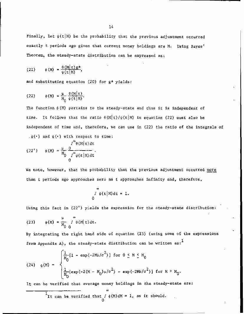
As is clear, the solution In equation (28) differs fundamentally from

the general solution in equation (7) which was obtained by minimizing the

present value of the cost of financial management. The most important differ-

ence is that the solution obtained by the steady—state approach does not depend

on the value of the variance which, In turn, plays a key role in the general

solution, It seems that, in this case, the adoption of a steady—state approach

results in an elimination of the effects of the stochastic characteristics of

the process governing money holdings. Thus, following the steady—state approach,

results in a fundamentally different interpretation of the determinants of optimal

money holdings. While the solution in equation (7) may be interpreted as con-

taining elements which pertain to both transactions and precautionary motives

for holding money, the solution in equation (28) contains only the deterministic

transaction motive. Obviously, in the special case for which a 0, the two

solutions coincide.1

The comparison of the two solutions in equation (7) and (28) also

raises a methodological question concerning the appropriateness of approximating

optimal adjustment policies by using a steady—state approach. The steady—state

approach is, of course, much simpler but unless one knows the true solution (as

in our case), the cost of obtaining simplicity cannot be assessed.

V. An Emp4lA lication toInternational Reserves

In this section we apply the model to an analysis of the holdings of

international reserves. In the empirical application we assume that the holdings

of international reserves are governed by the stochastic process in equation (1)

is indicated by Arrow et al (1958, p. 35) the two methods yieldidentical results vhen the rate of interest is zero. It implies that thedifference between the two methods arises due to the discounting involved inthe present value computation. A comparison of equation (8) and (24) with azero rate of interest illustrates the point.

18

with no drift (p = 0). Thus, we assume that on average the balance of payments

is balanced.1 Our assumption that adjustment occurs when reserves reach a

lower bound rather than an upper bound, seems to be especially appropriate for

the analysis of international reserves. The asymmetry in the division of the

burden of adjustment is well known; typically, adjustment is forced on the

deficit countries rather than on the surplus countries.

The previous analysis implies that, for the special case of no drift,

the optimal level of reserves (following an adjustment) is R0 (equation (10'),

Section II):

(29) =

Since in this case the steady—state distribution does not exist, we have assumed

in the empirical analysis that the observed data correspond to countries which

have adjusted recently. We have pooled cross—section and time series (annual)

data for 22 developed countries over five years (1971—75) and have estimated the

parameters of equation (30):2

(30) £nRb0+b1inci+b2nr+u

where u denotes an error term. The predictions of the model are that b1 .50

and that b2 = —.25.

For the purpose of estimation, international reserves are defined as the

sum of gold, Special Drawing Rights, foreign exchange, and reserve position at the

1For analysis emphasizing the stochastic properties of the time series ofinternational reserves, see Archibald and Richmond (1971), Heller (1966) andKenen and Yudin (1965); for analyses of international reserves in the context of

inventory models, see Makin (1974) and Olivera (1969).

2The classification of countries as "developed" is based on the Inter-national Monetary Fund. All data sources are from the IFS tape, obtained fromthe International Monetary Fund. We are indebted to Craig Hakkio for assistance

in the estimations.

19

Fund. The variability measure, a, is computed for each year as the standard

error (over the previous 15 years) of the trend—adjusted annual changes in the

stock of international reserves. The rate of interest is the government bond

yield or (depending on availability) the discount rate (except for Japan for

which we use the call—money rate).

In estimating equation (30) we allowed for a separate constant term for

each country. The least—squares parameter estimates are reported in equation

(31) and the various country—specific constant terms are reported in Table 1

with standard errors in parentheses below each coefficient.

(31) nR=b0+.505inc— .279Lnr(.110) (.149)

i2 = .975, n = 110, s.e. = 234

As may be seen, for that period, the estimated elasticities of reserve

holdings with respect to a and r are extremely close to the predictions of the

theoretical model. It is noted, however, that these results should be viewed

with caution since they might be sensitive to the omission of a scale variable

from the specification of equation (30). Furthermore, it has been shown in

Frenkel (1978) that the function which includes a scale variable but which

excludes the rate of interest, underwent a structural change by the end of 1972

and, therefore, the pooling of data from the period prior to 1973 with data from

the subsequent period might not have been appropriate. To examine the implications

of this possibility, we added a scale variable (meausred by the level of imports, IM)

and reestimated the resulting equation over the period 1963—72 (n = 198). The

resulting estimates are reported in equation (31'); the country—specific constant

terms (which are all significant) are not reported here.

(31') Zn R b0 + .676 Zn a — .233 Zn r + .352 Zn IN.

(.063) (.141) (.102)

20

TABLE 1

LEAST—SQUARES ESTIMATES OF COUNTRY—SPECIFICCONSTANT TERMS: 1971—75

(standard errors in parentheses)

United Kingdom 5.621 Japan 6.084(.731) (.787)

Austria 5.882 Finland 4.731(.511) (.456)

Belgium 6.010 Greece 4.931(.562) (.472)

Denmark 5.008 Iceland 3.420(.498) (.298)

France 6.115 Ireland 5.361(.703) (.459)

Germany 6.783 Portugal 5.489

(.780) (.514)

Italy 6.076 Spain 5.853

(.622) (.627)

Netherlands 6.1.95 turkey 5.096

(.584) (.528)

Norway 5.564 Australia 5.536

(.457) (.655)

Sweden 5.294 New Zealand 4.522

(.544) (.471)

Switzerland 6.420 South Africa 4.742

(.603) (.553)

Note: These are the constant terms corresponding to equation (31) in the text.

21

We conclude this section by stating that, on the whole, the empirical

results are consistent with the model. However, since the estimated parameters

seem to be somewhat sensitive to the specification and to the choice of the

time period, they should be interpreted only as illustrativeJ

VI. Concluding Remarks

In this paper we developed a stochastic framework for the analysis of

transactions and precautionary demand for money and we attempted to integrate

some aspects of previous contributions by Baumol (1952), Tohin (1956) and Miller

and Orr (1966). We derived formally the solution for optimal money holdings as

a function of the rate of interest, the mean rate of net disbursements, the cost

of portfolio adjustment, and the variance of the stochastic process governing

net disbursements. We also analyzed the determinants of the optimal length of

time elapsing between two consecutive portfolio adjustments. We then followed

the more traditional approach and analyzed the steady—state distribution of money

holdings and derived the optimal money stock that is implied by the steady—state

approach. A comparison of the two solutions illustrated that the two approaches

may yield solutions which differ significantly from each other. This comparison

led to the methodological question concerning the appropriateness of approximating

optimal adjustment policies by following the steady—state approach. We concluded

the analysis by applying the model to an empirical examination of countries'

holdings of international reserves. The analysis of the demand for international

reserves illustrated some of the potentially useful applications of the model.

1This statement is based on our own experimentation with different specifi-cations as well as on other studies. As is well known, other studies usingdifferent specifications and different time periods have encountered difficultiesin incorporating the rate of interest in the estimated reserve equation. Forreferences and details, see Frenkel (1978).

22

APPENDIX

Mathematical Derivations

In part A of this Appendix we derive equation (3') in the text and in

part B we show that the approximation involved in the derivation of equation (7)

introduces a negligible error.

Part A

We have assumed that money holdings are governed by the stochastic equation:

(A.l) dM(t) —pUt + adw(t); M(0) =M0.

In order to correspond with Cox and Miller's framework (1965, Ch. 5.7) in which

the first passage is for a process which starts at zero and goes through a

positive boundary, we perform the following transformations. Define

(A.2) dM(t) = pdt — adw(t); M(0) = — N0.

and

(A.3) dx(t) = pdt — crdw(t); x(0) = 0.

Thus, 14(t) is the mirror image of M(t) in the negative half—plane, and x(t)

M(t) + M0.

Let h(M, ti—H0, 0) be the probability that 14(t) (defined by equation (A.2)),

will not reach zero before period t, and that M(t) = M. Then equation (3) in the

text becomes

cc

(A.4) J1(140) = -ri ett(i }lh(M, ti—M0, 0)dN}dt.0 -

Analogously, in order to shift the origin so as to conform with Cox and Miller's

framework, let h*(x, tb, M) be the probability that x(t) will not reach the

boundary before t, and that x (t) = x• Since x (t) = M(t) + the relationship

23

between. h*() and h() is:

(A.5) h*(x, tJo, N3) h(x — N0, tJ—M0, 0).

In order to use the function h*(.), we change the variables in (A.4) by substi-

tuting x = M +N0:

N

(A.6) J1(M0) rfe"{f (x — N0)h(x —N0, t— N0, 0)dx}dt,

and using (A.5) in (A.6) results in:

(A.7) 31(M0)_rfet{iO (x - M0)h*(x, tjo, M0)dx)dt.

Decomposing (A.7) into expressions which involve N0 and expressiotwhich involve

x, yields:

(A.8) J1(M0) = rN0 f et[fO t0, N0)dx}dt —

—rJ 8rt{f xh(x, t0, M0)dx}dt.

Let f(M0, t) be the probability that x(t) will reach for the first time at

t. To simplify the notation, we will refer to this probability as f(t). Thus,

f(t) is also the probability that M(t) reaches zero for the first time at t;

therefore, the ptobability that the process will reach zero prior to t is:

t

F(t) .1 f(s)ds.0

It follows that the probability of not reaching zero prior to period t is:

h*(x, tb, M3)dx = 1 — F(t).

Using this result to evaluate the first integral in (A.8) yields:

24

(A.8.i) Jre rt1 — F(tfldt = [e_rt(l — F(t))] - fetf(t)dt.

Ccx and MIller (1965, Ch. 5.7) show that:

—rtf e (f)dt = a, where

h*(x, tb, ) = 1/

[exp{@—

Pt)2) — exp{o —

2nat 2at a

Substituting into (A.8) and integrating by parts yields

(A.9) 31(M0) = ? +frtD()d

where

—M0—pt 2pM M —ptD(t) = N[ 1/2 )exp( 20 } — N[

0

1/2at a at

x 2

NOt) 51 (2ir)1 ;Z /2dz.

Integrating by parts yields equation (3') in the text.

0

a exp{— Mo((2 + 2ra2)U2 -

substituting in (A.8.i) yields:

(A.8.ii) / re (/0 h*(x, t0, M0)dx)dt 1 — a.

We turn now to evaluate the second integral in (AS). Ccx and Miller (1965, Ch.

5.7) show that

(x —2740

— Pt)2

202 t

and where

25

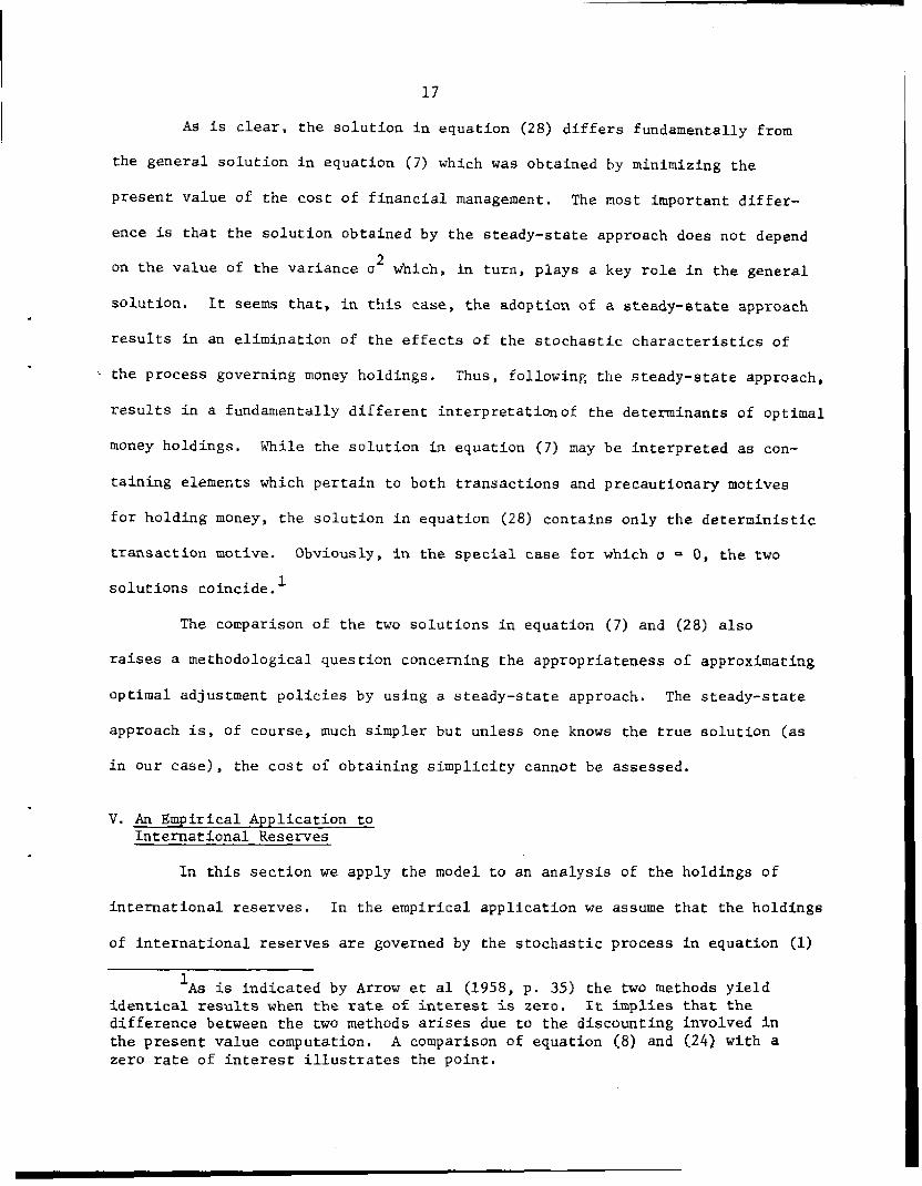
Part B

The necessary condition for optimization is:

(8.1) (1-caj+(M0 +C)---0.

Multiplying through by S E 1/a and noting that Ba/aM0 s —lox where a is

defined by equation (3') in the text and. where k .L_[(12 + 2rc2)V2 — ' 0,(8.1) becomes;

(8.1') —k(M0 + C) ÷ 5 — 1 = 0.

Taylor's Theorem with remainder implies that for some constant

A(0 'C c 1), the term in (3.1') can be expanded as:

(3.2) 5 5(Q) + 38(0M0 + M2 + * M.

03M0

Substituting a quadratic expansion of 5 (without the third order term) into (3.1')

yields:

(8.3) —k(M0 + C) + (Q) M0 +1 M = 0

(since 5(0) 1) and the solution for M0 is given in equation (7) in the text.

Using (8.1') and (8.2), the true solution for M0, which we denote by H, satisfies

equation (8.4);

(8.4) —k(R + C) + (°) + 4325jQ) 2 + 1 33s(Ai) 0

U

To determine the extent of the error involved in the approximation1 we subtract

(3.2) from (3.4) and cancel terms to obtain:

(5.5) 4(i2 — M+ 4k exp{Aik)t3= 0

26

since

S (0) = k, 0) = k2, and = ic exp(Xk}.0

Equation (8.5) impLies that

____ k - -—2 - exp(AMk}M > 0M

and, therefore, the approximate solution M0, exceeds the true solution E1.

Substituting FL0 for H yields the following inequalities:

H-H Mk(8.6) 0 <

< - exp{#\F10k}M0C 4 e

0

H0

where the last inequality follows since 0 C A < 1. Since equation (7) in the

text states that:

H0 = (2C)2kI2,(A.12) becomes

(8.6') 0 CH_R2

< (2kC)2e,Q{(2kc)U2).

Thus, the relative error is negligible if kG is negligible. From equation (7)

in the text, k = 2C/N and, therefore,

kG 2(f)2 < 2(.)0 14where c/si is the "broker's fee" divided by the true optimum H. As a practical

matter, for any reasonable o1er of magnitudes, the ratio C/H must be a very small

fraction and its square must be negligible and so is kG. Thus, the solution for

the optimum that is given by equation (7) is a good approximation to the true

solution.

27

REFERENCES

Archibald, G. C. and Richmond, J. "On the Theory of Foreign Exchange ReserveRequirements." The Review of Economic Studies 38, no. 2 (April 1971):245—6 3.

Arrow, K. J.; Karlin, S. and Scarf, H. Studies in the Mathematical Theory ofInventory and Production. Stanford: Stanford University Press, 1958.

Barro, Robert J. "Inflation, the Payment Period and the Demand for Money."Journal of Political Econopy 78, no. 6 (November/December 1970): l228-63.

Baumol, William J. "The Transactions Demand for Cash: An Inventory TheoreticalApproach." Quarterly Journal of Economics 66, no. 4 (November 1952):545—56.

Cox, R. B. and Miller, H.D. The Theory of Stochastic Processes. London:Methuen Ltd., 1965.

Feller, W. An Introduction to Probability and Its 4pplication, Vol. II, 2nd. ed.New York: Wiley, 1971.

Fischer, Stanley. "The Demand for Index Bonds." Journal of Political Economy83, no. 3 (June 1975): 509—34.

Frenkel, Jacob A. "International Reserves: Pegged Exchange Rates and ManagedFloat." In Brunner, K. and Meltzer, A.H. (eds..) Economic Policies inOpen Economies, Vol. 9 of the Carnegie—Rochester Conference Series onPublic Policy, a Supplementary Series to the Journal of MonetaryEconomics (July 1978).

Heller, Robert H. "Optimal International Reserves." Economic Journal 76(June 1966): 296—311.

Karni, Edi. "The Transactions Demand for Cash: Incorporating the Value of Timeinto the Inventory Approach." Journal of Political Economy 81, no. 5(September/October, 1973): 1216—25.

Kenen, Peter B. and Yudin, Elinor B. "The Demand for International Reserves."Review of Economics and Statistics 47 (August 1965): 242—50.

Makin, John H. "Exchange Rate Flexibility and the Demand for InternationalReserves." Weltwirtschaftliches Archiv 110, no. 2 (1974): 229—43.

Miller, Merton H. and Orr, Daniel. "A Model of the Demand for Money by Fins."Qparterly Journal of Economics 80, no. 3 (August 1966): 413—35.

Olivera, Julio H. G. "A Note on the Optimal Rate of Growth of InternationalReserves." Journal of Political Economy 77, no. 2 (March/April 1969): 245—48.

28

Olivera, Julio H.C. "The Scuare—Root Law of Precautionary Reserves." Journalof Political Economy 79, no. 5 (September/October): 1095—1104.

Orr, Daniel. Cash Management and the Demand for Money. New York: Praeger, 1970.

Patinkin, Don. Money Interest and Prices, 2nd ed. New York: Harper & Row, 1965.

Tobin, James. "The Interest—Elasticity of Transactions Demand for Cash."Review of Economics and Statistics 38, no. 3 (August 1956): 241—7.

Tsiang0 S. C. "The Precautionary Demand for Money: An Inventory TheoreticalAnalysis." Journal of Political Economy 77, no. 1 (January/February,1969): 99—117.

Whalen, Edward L. "A Rationalization of the Precautionary Demand for Cash."Qj.iarterly Journal of Ecoiomics 80, no. 2 (May 1966): 314—24.