SHAPE DEFORMATION STATISTICS AND REGIONAL TEXTURE-BASEDAPPEARANCE MODELS FOR SEGMENTATION

Jared Vicory

A dissertation submitted to the faculty of the University of North Carolina at Chapel Hill inpartial fulfillment of the requirements for the degree of Doctor of Philosophy in the Department

of Computer Science.

Chapel Hill2016

Approved by:

Stephen M. Pizer

Marc Niethammer

J. S. Marron

Beatriz Paniagua

Aaron Fenster

c© 2016Jared Vicory

ALL RIGHTS RESERVED

ii

ABSTRACT

JARED VICORY: Shape Deformation Statistics and Regional Texture-Based Appearance Modelsfor Segmentation.

(Under the direction of Stephen M. Pizer)

Transferring identified regions of interest (ROIs) from planning-time MRI images to the trans-

rectal ultrasound (TRUS) images used to guide prostate biopsy is difficult because of the large

difference in appearance between the two modalities as well as the deformation of the prostate’s

shape caused by the TRUS transducer. This dissertation describes methods for addressing these

difficulties by both estimating a patient’s prostate shape after the transducer is applied and then

locating it in the TRUS image using skeletal models (s-reps) of prostate shapes.

First, I introduce a geometrically-based method for interpolating discretely sampled s-reps into

continuous objects. This interpolation is important for many tasks involving s-reps, including

fitting them to new objects as well as the later applications described in this dissertation. This

method is shown to be accurate for ellipsoids where an analytical solution is known.

Next, I create a method for estimating a probability distribution on the difference between two

shapes. Because s-reps live in a high-dimensional curved space, I use Principal Nested Spheres

(PNS) to transform these representations to instead live in a flat space where standard techniques

can be applied. This method is shown effective both on synthetic data as well as for modeling the

deformation caused by the TRUS transducer to the prostate.

In cases where appearance is described via a large number of parameters, such as intensity

combined with multiple texture features, it is computationally beneficial to be able to turn these

large tuples of descriptors into a scalar value. Using the inherent localization properties of s-

reps, I develop a method for using regionally-trained classifiers to turn appearance tuples into the

probability that the appearance tuple in question came from inside the prostate boundary. This

iii

method is shown to be able to accurately discern inside appearances from outside appearances

over a large majority of the prostate boundary.

Finally, I combine these techniques into a deformable model-based segmentation framework

to segment the prostate in TRUS. By applying the learned mean deformation to a patient’s prostate

and then deforming it so that voxels with high probability of coming from the prostate’s interior

are also in the model’s interior, I am able to generate prostate segmentations which are comparable

to state of the art methods.

iv

To my friends and family.

v

ACKNOWLEDGMENTS

I would like to express my sincere thanks to everyone who has made my time at UNC and

in Chapel Hill so special. First I thank my advisor, Steve Pizer, for his wisdom and guidance

over these past several years without which this work would not have been possible. I thank the

other members of my dissertation committee: Steve Marron, Marc Niethammer, Beatriz Paniagua,

and Aaron Fenster, for their advice and support. I thank Jim Damon for his help with much of

the math behind s-reps and spoke interpolation over the years. I thank Aaron Ward for his help

with acquiring and analyzing the prostate data used in this research. I thank the departments of

Computer Science and Radiation Oncology for their financial support, with special mention of

Julian Rosenman and Gregg Tracton for their help with various projects over the years. I thank

Mark Foskey and Derek Merck for their early work and helpful advice on the project which is

the main area of this dissertation. I would like to give special mention to JP, Juan, Liyun, Chong,

Bingjie, Wenqi, Dibyendu, Xiaojie and others, for we share a special bond born from the shared

suffering that is Pablo. Finally, I thank all of my friends and family for their love and support over

the years.

vi

TABLE OF CONTENTS

LIST OF FIGURES . . . . . . . . . . . . . . . . . . . . . . . . . . . . . . . . . . . . . . . . . . . . . . . . . . . . . . . . . . . . . . . . . . . . . . . . . . . . . . . . . x

LIST OF ABBREVIATIONS . . . . . . . . . . . . . . . . . . . . . . . . . . . . . . . . . . . . . . . . . . . . . . . . . . . . . . . . . . . . . . . . . . . . . . . xi

1 INTRODUCTION . . . . . . . . . . . . . . . . . . . . . . . . . . . . . . . . . . . . . . . . . . . . . . . . . . . . . . . . . . . . . . . . . . . . . . . . . . . . . . . . 1

1.1 Image-guided Prostate Biopsy . . . . . . . . . . . . . . . . . . . . . . . . . . . . . . . . . . . . . . . . . . . . . . . . . . . . . . . . . . . . . . . . . 2

1.2 Segmentation of the Prostate from TRUS . . . . . . . . . . . . . . . . . . . . . . . . . . . . . . . . . . . . . . . . . . . . . . . . . . . . . 3

1.3 Skeletal Representations . . . . . . . . . . . . . . . . . . . . . . . . . . . . . . . . . . . . . . . . . . . . . . . . . . . . . . . . . . . . . . . . . . . . . . . 3

1.4 Statistics on Shape Differences . . . . . . . . . . . . . . . . . . . . . . . . . . . . . . . . . . . . . . . . . . . . . . . . . . . . . . . . . . . . . . . . 4

1.5 Appearance via Regional Texture Classifiers . . . . . . . . . . . . . . . . . . . . . . . . . . . . . . . . . . . . . . . . . . . . . . . . . 5

1.6 Interpolation of Discrete S-reps . . . . . . . . . . . . . . . . . . . . . . . . . . . . . . . . . . . . . . . . . . . . . . . . . . . . . . . . . . . . . . . . 6

1.7 Thesis & Contributions . . . . . . . . . . . . . . . . . . . . . . . . . . . . . . . . . . . . . . . . . . . . . . . . . . . . . . . . . . . . . . . . . . . . . . . . . 6

2 BACKGROUND. . . . . . . . . . . . . . . . . . . . . . . . . . . . . . . . . . . . . . . . . . . . . . . . . . . . . . . . . . . . . . . . . . . . . . . . . . . . . . . . . . 9

2.1 Object Representations . . . . . . . . . . . . . . . . . . . . . . . . . . . . . . . . . . . . . . . . . . . . . . . . . . . . . . . . . . . . . . . . . . . . . . . . . 9

2.1.1 Point Distribution Models . . . . . . . . . . . . . . . . . . . . . . . . . . . . . . . . . . . . . . . . . . . . . . . . . . . . . . . . . . . . . . . . . . . . 9

2.1.2 Skeletal Representations . . . . . . . . . . . . . . . . . . . . . . . . . . . . . . . . . . . . . . . . . . . . . . . . . . . . . . . . . . . . . . . . . . . . . 9

2.2 Statistical Methods . . . . . . . . . . . . . . . . . . . . . . . . . . . . . . . . . . . . . . . . . . . . . . . . . . . . . . . . . . . . . . . . . . . . . . . . . . . . . 10

2.2.1 Principal Component Analysis. . . . . . . . . . . . . . . . . . . . . . . . . . . . . . . . . . . . . . . . . . . . . . . . . . . . . . . . . . . . . . . 10

2.2.2 Non-linear Statistical Methods. . . . . . . . . . . . . . . . . . . . . . . . . . . . . . . . . . . . . . . . . . . . . . . . . . . . . . . . . . . . . . . 11

2.2.3 Principal Nested Spheres . . . . . . . . . . . . . . . . . . . . . . . . . . . . . . . . . . . . . . . . . . . . . . . . . . . . . . . . . . . . . . . . . . . . . 13

2.2.4 Composite Principal Nested Spheres . . . . . . . . . . . . . . . . . . . . . . . . . . . . . . . . . . . . . . . . . . . . . . . . . . . . . . . . 13

2.2.5 Appearance Models and Segmentation . . . . . . . . . . . . . . . . . . . . . . . . . . . . . . . . . . . . . . . . . . . . . . . . . . . . . . 14

2.2.6 Appearance-based Segmentation . . . . . . . . . . . . . . . . . . . . . . . . . . . . . . . . . . . . . . . . . . . . . . . . . . . . . . . . . . . . 14

2.2.7 Model-based Segmentation . . . . . . . . . . . . . . . . . . . . . . . . . . . . . . . . . . . . . . . . . . . . . . . . . . . . . . . . . . . . . . . . . . 16

vii

3 CONTINUOUS INTERPOLATION OF SKELETAL REPRESENTATIONS . . . . . . . . . . . . . . . . 19

3.1 Introduction . . . . . . . . . . . . . . . . . . . . . . . . . . . . . . . . . . . . . . . . . . . . . . . . . . . . . . . . . . . . . . . . . . . . . . . . . . . . . . . . . . . . . 19

3.2 Mathematics of Skeletal Representations . . . . . . . . . . . . . . . . . . . . . . . . . . . . . . . . . . . . . . . . . . . . . . . . . . . . . 21

3.3 Skeleton Interpolation . . . . . . . . . . . . . . . . . . . . . . . . . . . . . . . . . . . . . . . . . . . . . . . . . . . . . . . . . . . . . . . . . . . . . . . . . . 23

3.4 Spoke Interpolation . . . . . . . . . . . . . . . . . . . . . . . . . . . . . . . . . . . . . . . . . . . . . . . . . . . . . . . . . . . . . . . . . . . . . . . . . . . . . 24

3.5 Estimation of Spoke Direction Derivatives via Quaternion Splines . . . . . . . . . . . . . . . . . . . . . . . . . . 26

3.6 Interpolation of the Crest . . . . . . . . . . . . . . . . . . . . . . . . . . . . . . . . . . . . . . . . . . . . . . . . . . . . . . . . . . . . . . . . . . . . . . . 28

3.7 Spoke Computation via Integration of Derivatives. . . . . . . . . . . . . . . . . . . . . . . . . . . . . . . . . . . . . . . . . . . . 29

3.8 Discussion . . . . . . . . . . . . . . . . . . . . . . . . . . . . . . . . . . . . . . . . . . . . . . . . . . . . . . . . . . . . . . . . . . . . . . . . . . . . . . . . . . . . . . 30

4 PROBABILITY DISTRIBUTION ESTIMATION OF SHAPE DIFFERENCES. . . . . . . . . . . . . 31

4.1 Introduction . . . . . . . . . . . . . . . . . . . . . . . . . . . . . . . . . . . . . . . . . . . . . . . . . . . . . . . . . . . . . . . . . . . . . . . . . . . . . . . . . . . . . 31

4.2 Related Work . . . . . . . . . . . . . . . . . . . . . . . . . . . . . . . . . . . . . . . . . . . . . . . . . . . . . . . . . . . . . . . . . . . . . . . . . . . . . . . . . . . 32

4.3 Methodology . . . . . . . . . . . . . . . . . . . . . . . . . . . . . . . . . . . . . . . . . . . . . . . . . . . . . . . . . . . . . . . . . . . . . . . . . . . . . . . . . . . . 33

4.3.1 Euclideanization . . . . . . . . . . . . . . . . . . . . . . . . . . . . . . . . . . . . . . . . . . . . . . . . . . . . . . . . . . . . . . . . . . . . . . . . . . . . . . 33

4.3.2 Probability Distribution Estimation. . . . . . . . . . . . . . . . . . . . . . . . . . . . . . . . . . . . . . . . . . . . . . . . . . . . . . . . . . 34

4.4 Evaluation . . . . . . . . . . . . . . . . . . . . . . . . . . . . . . . . . . . . . . . . . . . . . . . . . . . . . . . . . . . . . . . . . . . . . . . . . . . . . . . . . . . . . . . 34

4.4.1 Single Mode of Change . . . . . . . . . . . . . . . . . . . . . . . . . . . . . . . . . . . . . . . . . . . . . . . . . . . . . . . . . . . . . . . . . . . . . . 35

4.4.2 Composed Bending and Twisting . . . . . . . . . . . . . . . . . . . . . . . . . . . . . . . . . . . . . . . . . . . . . . . . . . . . . . . . . . . . 36

4.4.3 Application to S-reps . . . . . . . . . . . . . . . . . . . . . . . . . . . . . . . . . . . . . . . . . . . . . . . . . . . . . . . . . . . . . . . . . . . . . . . . . 37

4.5 Discussion . . . . . . . . . . . . . . . . . . . . . . . . . . . . . . . . . . . . . . . . . . . . . . . . . . . . . . . . . . . . . . . . . . . . . . . . . . . . . . . . . . . . . . 37

5 MODELING TRUS APPEARANCE VIA REGIONAL TEXTURE CLASSIFIERS . . . . . . . . 40

5.1 Introduction . . . . . . . . . . . . . . . . . . . . . . . . . . . . . . . . . . . . . . . . . . . . . . . . . . . . . . . . . . . . . . . . . . . . . . . . . . . . . . . . . . . . . 40

5.2 Materials . . . . . . . . . . . . . . . . . . . . . . . . . . . . . . . . . . . . . . . . . . . . . . . . . . . . . . . . . . . . . . . . . . . . . . . . . . . . . . . . . . . . . . . . 41

5.3 Methodology . . . . . . . . . . . . . . . . . . . . . . . . . . . . . . . . . . . . . . . . . . . . . . . . . . . . . . . . . . . . . . . . . . . . . . . . . . . . . . . . . . . . 42

5.4 Application. . . . . . . . . . . . . . . . . . . . . . . . . . . . . . . . . . . . . . . . . . . . . . . . . . . . . . . . . . . . . . . . . . . . . . . . . . . . . . . . . . . . . . 43

5.4.1 Ultrasound Appearance Model . . . . . . . . . . . . . . . . . . . . . . . . . . . . . . . . . . . . . . . . . . . . . . . . . . . . . . . . . . . . . . 43

viii

5.5 Evaluation . . . . . . . . . . . . . . . . . . . . . . . . . . . . . . . . . . . . . . . . . . . . . . . . . . . . . . . . . . . . . . . . . . . . . . . . . . . . . . . . . . . . . . . 44

5.6 Discussion . . . . . . . . . . . . . . . . . . . . . . . . . . . . . . . . . . . . . . . . . . . . . . . . . . . . . . . . . . . . . . . . . . . . . . . . . . . . . . . . . . . . . . 45

6 SEGMENTATION OF THE PROSTATE FROM TRUS . . . . . . . . . . . . . . . . . . . . . . . . . . . . . . . . . . . . . . . 47

6.1 Introduction . . . . . . . . . . . . . . . . . . . . . . . . . . . . . . . . . . . . . . . . . . . . . . . . . . . . . . . . . . . . . . . . . . . . . . . . . . . . . . . . . . . . . 47

6.2 Materials . . . . . . . . . . . . . . . . . . . . . . . . . . . . . . . . . . . . . . . . . . . . . . . . . . . . . . . . . . . . . . . . . . . . . . . . . . . . . . . . . . . . . . . . 47

6.3 Segmentation Methodology . . . . . . . . . . . . . . . . . . . . . . . . . . . . . . . . . . . . . . . . . . . . . . . . . . . . . . . . . . . . . . . . . . . . 47

6.3.1 Model Deformation and Probability . . . . . . . . . . . . . . . . . . . . . . . . . . . . . . . . . . . . . . . . . . . . . . . . . . . . . . . . . 48

6.3.2 Probability Images and Image Match. . . . . . . . . . . . . . . . . . . . . . . . . . . . . . . . . . . . . . . . . . . . . . . . . . . . . . . . 49

6.3.3 Optimization . . . . . . . . . . . . . . . . . . . . . . . . . . . . . . . . . . . . . . . . . . . . . . . . . . . . . . . . . . . . . . . . . . . . . . . . . . . . . . . . . . 50

6.4 Results . . . . . . . . . . . . . . . . . . . . . . . . . . . . . . . . . . . . . . . . . . . . . . . . . . . . . . . . . . . . . . . . . . . . . . . . . . . . . . . . . . . . . . . . . . 50

6.4.1 Estimation of Prostate Deformation Distribution . . . . . . . . . . . . . . . . . . . . . . . . . . . . . . . . . . . . . . . . . . . 50

6.4.2 Segmentation . . . . . . . . . . . . . . . . . . . . . . . . . . . . . . . . . . . . . . . . . . . . . . . . . . . . . . . . . . . . . . . . . . . . . . . . . . . . . . . . . 50

6.4.3 Refinement . . . . . . . . . . . . . . . . . . . . . . . . . . . . . . . . . . . . . . . . . . . . . . . . . . . . . . . . . . . . . . . . . . . . . . . . . . . . . . . . . . . . 51

6.5 Discussion . . . . . . . . . . . . . . . . . . . . . . . . . . . . . . . . . . . . . . . . . . . . . . . . . . . . . . . . . . . . . . . . . . . . . . . . . . . . . . . . . . . . . . 52

7 CONCLUSIONS & DISCUSSION . . . . . . . . . . . . . . . . . . . . . . . . . . . . . . . . . . . . . . . . . . . . . . . . . . . . . . . . . . . . . 54

7.1 Discussion and Future Work . . . . . . . . . . . . . . . . . . . . . . . . . . . . . . . . . . . . . . . . . . . . . . . . . . . . . . . . . . . . . . . . . . . 55

7.1.1 S-reps and Fitting . . . . . . . . . . . . . . . . . . . . . . . . . . . . . . . . . . . . . . . . . . . . . . . . . . . . . . . . . . . . . . . . . . . . . . . . . . . . . 55

7.1.2 Interpolation . . . . . . . . . . . . . . . . . . . . . . . . . . . . . . . . . . . . . . . . . . . . . . . . . . . . . . . . . . . . . . . . . . . . . . . . . . . . . . . . . . 56

7.1.3 Statistics on Shape Differences . . . . . . . . . . . . . . . . . . . . . . . . . . . . . . . . . . . . . . . . . . . . . . . . . . . . . . . . . . . . . . 57

7.1.4 Appearance Model . . . . . . . . . . . . . . . . . . . . . . . . . . . . . . . . . . . . . . . . . . . . . . . . . . . . . . . . . . . . . . . . . . . . . . . . . . . 58

7.1.5 Segmentation . . . . . . . . . . . . . . . . . . . . . . . . . . . . . . . . . . . . . . . . . . . . . . . . . . . . . . . . . . . . . . . . . . . . . . . . . . . . . . . . . 58

7.1.6 Conclusions . . . . . . . . . . . . . . . . . . . . . . . . . . . . . . . . . . . . . . . . . . . . . . . . . . . . . . . . . . . . . . . . . . . . . . . . . . . . . . . . . . . 60

REFERENCES . . . . . . . . . . . . . . . . . . . . . . . . . . . . . . . . . . . . . . . . . . . . . . . . . . . . . . . . . . . . . . . . . . . . . . . . . . . . . . . . . . . . . . 61

ix

LIST OF FIGURES

2.1 Euclidean vs non-Euclidean mean . . . . . . . . . . . . . . . . . . . . . . . . . . . . . . . . . . . . . . . . . . . . . . . . . . . . . . . . . . . . . 12

2.2 PNS projection example. . . . . . . . . . . . . . . . . . . . . . . . . . . . . . . . . . . . . . . . . . . . . . . . . . . . . . . . . . . . . . . . . . . . . . . . 13

3.1 Usefulness of s-rep interpolation for fitting . . . . . . . . . . . . . . . . . . . . . . . . . . . . . . . . . . . . . . . . . . . . . . . . . . . 19

3.2 S-rep spoke-relative dilation . . . . . . . . . . . . . . . . . . . . . . . . . . . . . . . . . . . . . . . . . . . . . . . . . . . . . . . . . . . . . . . . . . . 23

3.3 Interpolated s-rep skeletal sheet. . . . . . . . . . . . . . . . . . . . . . . . . . . . . . . . . . . . . . . . . . . . . . . . . . . . . . . . . . . . . . . . 24

3.4 S-rep interpolation quad . . . . . . . . . . . . . . . . . . . . . . . . . . . . . . . . . . . . . . . . . . . . . . . . . . . . . . . . . . . . . . . . . . . . . . . . 25

3.5 De Casteljau’s algorithm . . . . . . . . . . . . . . . . . . . . . . . . . . . . . . . . . . . . . . . . . . . . . . . . . . . . . . . . . . . . . . . . . . . . . . . 27

3.6 Crest curve dilation for interpolation . . . . . . . . . . . . . . . . . . . . . . . . . . . . . . . . . . . . . . . . . . . . . . . . . . . . . . . . . . 29

3.7 An interpolated s-rep . . . . . . . . . . . . . . . . . . . . . . . . . . . . . . . . . . . . . . . . . . . . . . . . . . . . . . . . . . . . . . . . . . . . . . . . . . . 30

4.1 Estimated bending and twisting angles . . . . . . . . . . . . . . . . . . . . . . . . . . . . . . . . . . . . . . . . . . . . . . . . . . . . . . . . 35

4.2 Difference between PCA- and CPNS-estimated deformations . . . . . . . . . . . . . . . . . . . . . . . . . . . . . . . 37

4.3 Mean deformations applied to s-reps . . . . . . . . . . . . . . . . . . . . . . . . . . . . . . . . . . . . . . . . . . . . . . . . . . . . . . . . . . 38

4.4 S-rep deformation eigenmodes. . . . . . . . . . . . . . . . . . . . . . . . . . . . . . . . . . . . . . . . . . . . . . . . . . . . . . . . . . . . . . . . . 39

5.1 Fanned and unfanned ultrasound images . . . . . . . . . . . . . . . . . . . . . . . . . . . . . . . . . . . . . . . . . . . . . . . . . . . . . . 44

5.2 Ultrasound intensity and texture images. . . . . . . . . . . . . . . . . . . . . . . . . . . . . . . . . . . . . . . . . . . . . . . . . . . . . . . 44

5.3 DiProPerm z-scores . . . . . . . . . . . . . . . . . . . . . . . . . . . . . . . . . . . . . . . . . . . . . . . . . . . . . . . . . . . . . . . . . . . . . . . . . . . . 45

5.4 Path misclassification rates . . . . . . . . . . . . . . . . . . . . . . . . . . . . . . . . . . . . . . . . . . . . . . . . . . . . . . . . . . . . . . . . . . . . . 45

6.1 Prostate probability image . . . . . . . . . . . . . . . . . . . . . . . . . . . . . . . . . . . . . . . . . . . . . . . . . . . . . . . . . . . . . . . . . . . . . 49

6.2 Prostate pre- and post-deformation . . . . . . . . . . . . . . . . . . . . . . . . . . . . . . . . . . . . . . . . . . . . . . . . . . . . . . . . . . . . 51

6.3 Results of segmentation method . . . . . . . . . . . . . . . . . . . . . . . . . . . . . . . . . . . . . . . . . . . . . . . . . . . . . . . . . . . . . . . 52

x

LIST OF ABBREVIATIONS

CPNS Composite Principal Nested Spheres

DSC Dice Similarity Coefficient

DWD Distance-weighted Discrimination

GPCA Geodesic Principal Component Analysis

LDDMM Large Deformation Diffeomorphic Metric Mapping

MAD Mean Absolute Distance

MRI Magnetic Resonance Imaging

MSE Mean Squared Error

PCA Principal Component Analysis

PDM Point Distribution Model

PGA Principal Geodesic Analysis

PNS Principal Nested Spheres

ROI Region of Interest

S-rep Skeletal Representation

SVM Support Vector Machine

TPS Thin Plate Spline

TRUS Trans-rectal Ultrasound

xi

1 INTRODUCTION

The driving problem for the work in this dissertation is segmentation of the prostate in 3D

trans-rectal ultrasound (TRUS) during an image-guided biopsy procedure. The main task is to

identify the prostate and certain regions of interest (ROIs) identified during pre-biopsy planning.

This problem presents several challenges, including

1. Low contrast between the prostate and surrounding tissue

2. High noise and noise-like (speckle) artifacts present in ultrasound

3. Highly varying appearance around the prostate boundary

4. Deformation of the prostate caused by the TRUS transducer

The first three items combine to make segmentation of the prostate challenging using standard tech-

niques which may work well in other imaging modalities. The fourth makes using prior knowledge

of the shape of a particular patient’s prostate gained during planning difficult as well as locating

corresponding regions of the prostate post-deformation.

I argue that a method designed to solve this driving problem needs

1. A model of shape that supports

• identification of corresponding local regions across multiple cases

• continuous representation of both the boundary and interior of the prostate

2. An appearance model that

• is defined locally rather than globally

1

• uses features suitable for analysis of ultrasound appearance, especially texture

3. Statistical analysis of the differences between pairs of shapes

This dissertation describes novel methodological contributions in each of these areas. The

following sections further develop the driving problem and the intuition behind each of the items

listed above.

1.1 Image-guided Prostate Biopsy

Prostate cancer is the most commonly diagnosed cancer among adult men (excluding basal cell

carcinoma) and is the second leading cause of cancer death among men in the United States [1].

Early diagnosis is important for improving survivability of prostate cancer. The standard method

for obtaining this diagnosis is through a TRUS-guided biopsy of the suspected cancer.

Often, the ROIs for the biopsy procedure are identified on an MRI of the pelvis. On MRI

there is typically good contrast in the soft tissue and relatively easy detection of ROIs. During the

biopsy procedure the available TRUS images are of very different appearance and quality than the

planning MRIs, making accurate identification of the ROIs difficult. Compounding this problem

is the fact that the TRUS transducer puts pressure on and deforms the prostate, causing it to have a

different shape compared to planning-time. These factors make TRUS-guided biopsy error-prone

and can lead to missing a significant fraction of cancers. In order to improve the accuracy of the

biopsy procedure, it is important to be able to accurately identify not only the prostate boundary in

TRUS but also regions of the prostate which correspond with MRI-identified ROIs.

A team led by Dr. Aaron Fenster at the Robarts Research Institute at Western University has

developed a system which allows for segmentation of the prostate from TRUS and registration

with a planning MR image to identify biopsy targets. They have shown that, when done correctly,

this approach can reduce the number of needle insertions needed to accurately diagnose prostate

cancer by up to half [2].

2

1.2 Segmentation of the Prostate from TRUS

Segmentation of the prostate in TRUS is most effectively done by analyzing the texture of

the image, whether on a global or local scale. Many of these methods also include some type of

shape prior in order to keep the segmented shape regular. Point distribution models (PDMs) [3] are

commonly used in shape-informed segmentation methods for the prostate as well as many other

organs throughout the body. These methods will often learn statistics on a population of PDMs

using principal component analysis (PCA) and restrict the set of candidate shapes to the space of

shapes spanned by some number of eigenmodes of this learned distribution.

PDMs have several useful properties, including ease of model creation, simplicity of represen-

tation, and straightforwardness of various computations involving their representation. The geom-

etry captured by PDMs, however, is somewhat limited, particularly when restricted to boundary

points only (as is often the case). Boundary PDMs capture only 0th-order information about the

object’s surface explicitly and thus lack higher-order information such as boundary normal direc-

tions or surface curvatures. These can be estimated if the surface has connectivity information,

but the accuracy will be limited by the sample density. Boundary PDMs also do not explicitly

model the object interior, which is important for applications needing corresponding locations in

the object’s interior.

1.3 Skeletal Representations

Skeletal representations model an object via a skeletal locus running through the interior of

an object and a non-crossing vector field defined on this skeleton and pointing to the object’s

boundary. Discrete skeletal representations, called s-reps, consist of samples of the interior skele-

ton, either two (interior samples) or three (exterior samples) vectors called spokes anchored at the

skeleton and pointing towards the boundary, and corresponding spoke lengths giving the distance

from the skeleton to the object boundary along each spoke [4]. Compared to boundary PDMs, this

representation offers several advantages. Most importantly, s-reps model the entire object interior

as opposed to just the boundary and include directional (1st order) information in addition to purely

3

position information about the object’s surface. This representation has been shown to be superior

to boundary PDMs for uses such as classification [5] and estimating object correspondences. [6].

Due to the non-Euclidean nature of most of an s-rep’s features, standard Euclidean statistical

methods such as PCA are not directly applicable to s-reps. Instead, an alternative approach called

Euclideanization is used to turn these non-Euclidean features into Euclidean ones to which stan-

dard methods can then be applied. This Euclideanization of the sphere-resident features is done

via principal nested spheres (PNS), which analyzes the s-rep features on the abstract spheres they

naturally live on. Performing PCA on these Euclideanized features yields an s-rep shape space

which can be used for segmentation as described previously.

1.4 Statistics on Shape Differences

As mentioned previously, the TRUS transducer causes the shape of the prostate to deform from

what is observed on the planning MRI. In segmenting the prostate from TRUS, I wish to leverage

information learned from a patient’s MRI. For this, it is not enough to simply learn a distribution of

shapes of the prostate post deformation; we must also learn how the transducer causes the prostate

to deform.

Given an MRI/TRUS image pair for a specific patient and manual segmentations of the prostate,

I can learn the transducer-induced deformation by fitting consistent s-reps to both segmentations

and computing a deformation from the MRI to the TRUS models. Given a population of such

pairs, a probability distribution of these shape changes can be learned. To do this in a meaningful

way, both the deformations and the probability distribution must be computed while keeping the

non-Euclidean nature of s-reps in mind.

In Euclidean space, differences between two points are easily computed by simple subtraction,

and probability distributions of these differences can again be estimated via PCA after translation

to the origin. For objects which live on a curved manifold, this procedure becomes less well-

defined. The difference between two points on a manifold is generally computed as a geodesic

along the surface between these two points, but depending on the manifold these geodesics can be

4

difficult and expensive to compute. Moreover, given a population of geodesics on the manifold,

they must first be transported to a common starting point before they can be compared, a far from

trivial task except in spaces where a closed-form solution is known.

Instead, because the exact structure of the manifold s-reps live on is known and there are statisti-

cal methods capable of analyzing them directly on this manifold, I again apply the Euclideanization

idea to computing the difference between two s-reps. Taking the pooled group of MRI and TRUS

prostate models, I compute PNS and thus a common polar system for Euclideanization. Then, the

Euclideanized s-reps can be directly analyzed in Euclidean space as described previously, yielding

a mean deformation and modes of deformation variation.

Given a new patient’s manually segmented MRI, I can apply this mean deformation to yield a

patient-specific intialization for the prostate’s shape in the TRUS image and deform it over these

modes of deformation variation to better match the image using some model of the prostate’s

appearance in TRUS.

1.5 Appearance via Regional Texture Classifiers

Analyzing the appearance of an organ in ultrasound imaging is a difficult task. Relying on

intensity information alone is unsatisfying because of issues of low contrast between neighboring

organs as well as the noise-like speckle artifacts found in ultrasound images. Instead, texture fea-

tures are often used to model the appearance of the prostate in TRUS images. Gabor filters, either

2D or 3D, are a common choice for this task. I compute texture using 48 oriented Gabor features

which, together with the smoothed image intensity, yields a 49-tuple of appearance information at

each image voxel.

However, this texture cannot be learned globally, as the texture of the areas surrounding the

prostate boundary vary widely around the object. Instead, I learn texture on a local scale. The

s-rep provides a natural method of defining local regions around the boundary of an object using

the spoke ends as landmarks, as the s-rep fitting process ensures reasonable correspondence over

a population of objects. By learning separate texture profiles on each s-rep spoke, I can be more

5

robust to the changes in TRUS appearance around the prostate than methods which model texture

globally or using large regions of the image.

I learn these local texture profiles by, about each spoke, pooling texture features from just

inside and just outside the prostate boundary into two classes and training a classifier to distinguish

between them. For a new case to be segmented, we apply these classifiers to the voxels near the

boundary of a candidate object and optimize the model so that more likely inside voxels are inside

the boundary and vice versa.

1.6 Interpolation of Discrete S-reps

For many applications, including the segmentation problem here, it is desirable to have a more

finely sampled s-rep than the base model. This is desirable for fitting an s-rep to an object. It is

also used for representing an object in terms of object-relative coordinates, which is an important

component for producing regional appearance models for segmentation. These objectives require

the development of a method for continuously interpolating a discrete s-rep. Building on the

calculus of skeletal models, I develop a geometry-based method for interpolating an s-rep into a

continuous object while maintaining its useful geometric properties.

1.7 Thesis & Contributions

Thesis: Segmentation of an object deformed from a base state in a systematic way with appear-

ance that varies around its boundary benefits from combining the following two approaches:

1. Statistical analysis of the object deformation by a method suited for analysis in curved spaces

2. Regionally trained appearance models to distinguish voxels inside and outside of the object’s

boundary.

Instead of the more typical boundary-based approach, continuously interpolated skeletal models

form a strong basis for the training of statistics of object deformation as well as the creation of

object-relative regions on which to train appearance models.

The major methodological contributions of this dissertation are as follows:

6

1. A geometric interpolation method for computing continuous skeletal models from discrete

s-rep models.

2. A method for computing a probability distribution of differences between pairs of shapes

which leverages the non-Euclidean nature of shape and shape representations.

3. A novel appearance model which leverages the ability of the s-rep to produce corresponding

local regions around an object to define local classifiers of image texture.

4. The application of the aforementioned techniques in a deformable model-based segmenta-

tion method for segmenting the prostate from TRUS.

In addition to these, I have also accomplished the following engineering contributions:

1. Implementation in Pablo, the main piece of software used to fit and visualize s-reps, of code

allowing optimization over a shape space defined by CPNS

2. Implementation in Pablo of spoke interpolation in both the display and fitting of s-reps

3. Implementation of code to compute and optimize over spaces of shape differences

4. Implementation to compute regional classifiers of inside/outside boundary appearance fea-

tures and computation of images of probability of being inside and object

5. Implementation in Pablo of code allowing optimization of a model to best fit a probability

image, including both optimization over a global shape space and local refinements

6. Numerous bug fixes and improvements to Pablo

The rest of this dissertation is laid out as follows. Chapter 2 gives background information

necessary to fully understand the following chapters, chapter 3 details and evalutes the s-rep spoke

interpolation method, chapter 4 describes and evalutes the method by which I compute probabil-

ity distributions of shape differences, chapter 5 describes and evaluates the s-rep-based regional

7

appearance model, chapter 6 describes the segmentation framework as applied to TRUS prostate

segmentation with an evaluation that emphasizes the statistical frameworks developed in the earlier

chapters, and chapter 7 contains concluding thoughts and discussion.

8

2 BACKGROUND

This section covers information which is common background information for each of the

following chapters. Background information specific to only one chapter can be found there.

2.1 Object Representations

2.1.1 Point Distribution Models

Point distribution models (PDMs) are shape models which are a collection of points which are

in corresponding locations on each object of a population. Though they are often formed using

only boundary points, they are not restricted to be so. There are several methods for producing

PDMs from a set of objects, including manual placement of landmarks, automatic generation of

corresponding points such as SPHARM-PDM [7], and methods for optimizing the correspondence

of existing models such as the entropy-based method of Cates [8].

2.1.2 Skeletal Representations

The s-rep is a quasi-medial skeletal model that models not only an objects boundary but its

interior as well. The s-rep is a collection of points sampled from a skeleton of an object which have

associated non-crossing vectors called spokes pointing from the skeleton to the objects boundary.

S-reps attempt to be as close to medial as possible while remaining non-branching and require the

spokes to touch the object boundary and be nearly orthogonal to it. These samples can then be

interpolated via the method described in chapter 3 to produce a continuous representation of an

objects boundary and interior. This provides an object-relative coordinate system (u, v, τ) for the

objects volume, where (u, v) parameterizes the skeleton and τ moves from the skeleton (τ = 0) to

the boundary (τ = 1).

S-reps are fit to an object via an optimization which tries to match the s-rep’s implied boundary

to an object while remaining as medial as possible. Current s-rep fitting is initialized via warping

9

a template model into an invidual case via a thin plate spine (TPS) interpolation of the boundary

correspondences of the template object and the target object followed by an optimization which

more closely matches the spokes to the object’s boundary. For producing these correspondences,

I use the thin shell demons [9] method to register a reference PDM to a target PDM and use the

implied correspondences to fuel the TPS warping.

In the past several years, s-reps have been shown to be powerful and in most cases superior

to PDMs for a variety of statistical tasks, including hypothesis testing [10], classification [5], and

producing corresponding objects [6].

2.2 Statistical Methods

2.2.1 Principal Component Analysis

Principal component analysis (PCA) is an important statistical procedure designed to be used

for probability distribution estimation and dimensionality reduction of Euclidean data. The result

of PCA on data of dimension d can be understood as the fitting of a d-dimensional Gaussian

distribution to the data.

PCA can operate in either a forward or backward manner, the results of which are equivalent

for Euclidean data. In the typical forward approach, the first step is to compute the mean of

the data, which is the best fitting linear subspace of dimension 0. The line through the mean

which minimizes the sum of the squared projections of each data point to the line, the best-fitting

subspace of dimension 1, is called the first principal component. Next, the plane containing the first

principal component which minimizes the projection error is computed. The vector contained by

this plane which is orthogonal to the first principal component is the second principal component.

This procedure of fiting the best-fitting linear subspace of successively increasing dimension is

repeated d times.

Instead of this approach which builds a set of best-fitting subspaces of increasing dimension,

an alternative method [11] is to start by fitting the best-fitting d−1 dimensional subspace (with the

direction orthogonal to it being the dth principal component), project the data onto it, and repeat

10

until d− 1 = 0, yielding a mean. In this approach, PCA can be thought of as a successive addition

of constraints to the original data rather than a construction of best-fitting lines as in the forward

approach. In a Euclidean space both approaches yield the same result, but this property does not

hold in general.

PCA can be computed by an eigendecomposition of the data covariance matrix. When sorted

from largest to smallest eigenvalue, the corresponding eigenvectors represent the principal com-

ponents in decreasing order, while the eigenvalues represent the variances of the 1-dimensional

Gaussians in orthogonal spaces which compose the overall distribution.

One of the most important characteristics of a PCA-generated probability distribution is having

as few large eigenvalues as possible given the data being analyzed. This typically indicates that the

data are well represented by a small number of linear subspaces, yielding strong dimensionality

reduction with low loss of information.

2.2.2 Non-linear Statistical Methods

PCA is a powerful analysis technique, but it assumes that the underlying data are samples from

some distribution on a flat space. However, if the data are instead samples from some curved man-

ifold, this assumption often causes PCA to produce distributions with many significant eigenval-

ues, meaning that many dimensions are needed to keep information loss adequately low. Modeling

manifold data using linear subspaces also yields data points outside of the original manifold. Fig-

ure 2.1 shows a simple example of computing the mean of two data points sampled from an arc of

a circle. In this case, the mean computed via a metric which knows about the manifold’s structure

is more appropriate than the traditional Euclidean mean.

In the area of statistical shape analysis, most of the data encountered live on curved manifolds.

While PCA is widely used in the analysis of PDMs, this approach is not ideal because it does not

take the structure of the underlying manifold into consideration and can yield ineffective analysis.

The use of more complex and powerful models such as s-reps only increases the deficiencies

inherent in this approach because of the increased complexity of the underlying manifold structure.

11

Figure 2.1: On the left, without knowledge of the data’s original manifold, the Euclidean mean(red point) is a good approximation. On the right, knowing the data are samples from an arc, themean using the manifold’s metric (blue point) is more reasonable.

Because of this, methods which can analyze data directly on their manifold are desired.

A popular method for analyzing data on a curved manifold is principal geodesic analysis

(PGA) [12]. In its most common form, PGA computes a mean of the data on the manifold. Then,

all of the data is mapped onto the tangent plane at the mean and PCA is computed on this projected

data.

Geodesic PCA (GPCA) [13] is a method which works similarly to PGA, but instead of using

PCA in the tangent space it instead minimizes projection error to geodesics on the manifold itself.

This method has the drawback that it needs explicit formulas for manifold geodesics, which are

often not available.

PGA and related methods work on data which live on some manifold which may not be easy

to work with directly. In cases where the underlying manifold is known, however, approaches

which can use this knowledge directly can produce more accurate and efficient results. Many

shape representations either are or are composed of data which live on abstract spheres, such as

PDMs [14] and s-reps [4].

Kendall [14] notes that PDMs comprised of n points, when translated to have center of mass

at the origin and scaled to unit length, are points on S3n−4 (3 degrees of freedom removed for

translation, 1 for scaling). In s-reps, the PDM which makes up the collection of skeletal samples

is a spherical entity, as well as the collection of unit spoke directions, each of which live on S2.

12

Because so many of these features are spherical, a method tailored to analyzing spherical data is

desirable.

2.2.3 Principal Nested Spheres

Principal nested spheres (PNS) [15] is a method that operates in a PCA-like backwards fashion

on spherical data. Starting from Sd, the best-fitting subsphere Sd−1 is computed and represented as

a pole w and angle ψ. Each point pi is projected onto the subsphere, and the process is repeated on

each subsphere until a single point, the backwards mean, is reached. At each projection step, the

signed geodesic distance Zd,1 from each point to the fit subspace is recorded, yielding d residuals

for each data point. These residuals are called the Euclideanized form of the data, while the

collection of poles and angles defining the subspheres form a polar system which can be used to

Euclideanize a new shape via this repeated projection. A Euclideanized shape can be returned to its

original ambient space by undoing these projections to recover the original representation. Figure

2.2 shows an example PNS step.

Figure 2.2: An example projection step from a PNS analysis. The point p1 is projected onto thesubsphere defined by the polar system A(w1, ψ1). The projection distance Zd,1 is a Euclideanizedfeature.

2.2.4 Composite Principal Nested Spheres

Because PNS transforms spherical data into Euclidean data, we can analyze its results using

standard Euclidean techniques such as PCA. S-reps are represented as a collection of hub points

which can be represented as a PDM along with many spokes, each of which has a length and direc-

tion. There are several different PNS analyses which must be done for s-reps: one to Euclideanize

13

the hub PDM and one for each s-rep spoke direction. For each s-rep, the resulting Euclideanized

values are combined with the log-transformed spoke lengths into a single vector Z in a step called

compositing. The collection of Z vectors for a population of s-reps can then be analyzed using

PCA. This technique is known as composite principal nested spheres (CPNS).

Experimentally, it has been shown that s-rep features, particularly spoke directions, tend to

lie on or near subspheres and are thus well modeled via PNS. CPNS has been shown to produce

more efficient representations and statistics for both PDMs and s-reps than either PCA or PGA,

leading to improved performance in tasks such as hypothesis testing [10] and classification [5].

These results indicate that CPNS-based Euclideanization is a powerful technique for the analysis

of s-reps.

2.2.5 Appearance Models and Segmentation

In this section, I discuss previous work on how to model image appearance for segmentation,

focusing on methods used for ultrasound prostate segmentation. I divide the methods into two

broad categories: those that attempt to segment an object via appearance directly, and those that

combine image information with some type of deformable model to perform segmentations. Full

surveys of prostate segmentation methods can be found in [16] and [17].

2.2.6 Appearance-based Segmentation

While the simplest method for modeling image appearance is by using the raw image intensity

values directly, it is rarely used due to the statistical variation of intensity features typical of medical

image aquisition, a problem which is particularly bad for ultrasound. The most straightforward

method of appearance modeling used in practice is to localize edges in an image using intensity

gradients and use these derived edges to directly segment the object of interest. These methods fail

in situations where there is low contrast or large amounts of noise or other artifacts, such as speckle

in ultrasound. There are several techniques which can be used to address these problems. Aarnink

et al. [18] used local standard deviations of intensity at multiple scales to identify homogeneous

regions in an image. Pathak et al. [19] used a stick filter to reduce speckle and enhance contrast

14

in the ultrasound image by using the fact that speckle is correlated over large distances. Mahdavi

et al. [20] use measures of edge strength in vibro-elastography (VE) ultrasound images rather than

typical B-mode images to perform segmentation. A common approach in all imaging modalities to

smooth image intensity while preserving edges is to use an anisotropic diffusion filter. In my work

on modeling ultrasound appearance in chapter 5, I use the speckle-reducing anisotropic diffusion

method of Yu et al.[21] to get smoothed ultrasound images.

Graph-based segmentation algorithms model image voxels or groups of voxels as nodes in a

graph. The edges linking a voxel to its neighbors have an associated cost, typically related to the

gradient of the image. The image is segmented by trying to cut the graph into different pieces

while minimizing the cost of these cuts. Zouqi et al. [22] used graph partitioning to segment the

prostate with the user defining seed points which act as the sink and source nodes for a max flow

optimziation. Qiu et al. [23] segment the prostate using a coherent continuous max-flow model

which enforces geometric consistency across multiple 2D slices to segment the prostate in 3D.

Classification of image voxels can be used to segment objects. These methods use supervised

machine learning techniques to train classifiers to distinguish between different classes of voxels.

Each voxel typically has associated with it a vector of features (including image intensity, texture,

physical features, etc.) with the hope of learning which features distinguish different groups of

voxels. Zaim et al. [24] used spatial locality and image texture in a self-organizing map to segment

the prostate from ultrasound. Zaim et al. [25] also used entropy and wavelet transform coefficients

to segment the prostate using an SVM. Mohammed et al. [26] used multi-resolution Gabor features

to identify ROIs and classify the ROIs based on various spectral features to obtain a segmentation.

Clustering-based methods have also been used for segmentation. Like the classification-based

methods, they also use feature vectors to represent voxels. Instead of attempting to determine if a

single voxel is from one class or another, they attempt to group voxels into different groups based

on these features with the goal of collecting all voxels from the particular object of interest into

one group. Richard et al. [27] use mean-shift on four texture features to perform segmentations by

15

determining the mean and covariance for each of a set of clusters and assigning a probability to

each voxel for each cluster. The object boundary was then refined using spatial information, with

spatially close voxels being more likely to have come from the same cluster.

2.2.7 Model-based Segmentation

The class of methods described in section 2.2.6 attempt to capture the boundary of an object

purely by considering its appearance and attempting to separate it from surrounding tissue. While

they have been successful in many applications, methods of this class can result in segmentations

which are non-smooth or possibly not even continuous, especially if they are working on a voxel-

by-voxel basis rather than considering spatial locality. To combat this problem, these methods

can be supplemented by models which can deform to match a boundary located by analyzing

an image’s appearance. Regularity constraints can be used in order to ensure that the resulting

boundaries are smooth and continuous while still closely matching the object of interest.

A common class of model-based methods are active contour models (ACMs). Initially devel-

oped by Kass et al. [28], ACMs or snakes can be represented as sequential sets of control points

connected by curves and can leverage many of the appearance analysis techniques described in

section 2.2.6 in order to locate an object’s boundary. They proceed by moving an initial contour

(via moving the control points) closer to the object rather than attempting to capture its edge di-

rectly such as the purely edge-detecting methods which, along with a regularization, guarantees

a smooth and continuous boundary for the object. Jendoubi et al. [29] used a gradient vector

flow model computed via a combination of Laplacian of Gaussian and Sobel operators to move

the ACM towards the prostate boundary and improve its capture range, lessening its reliance on

accurate initialization. ACMs can also work with more complex methods of modeling of image

appearance. Knoll et al. [30] used the dyadic wavelet transform to determine prostate edges and

deform an ACM to match the prostate boundary. Zaim et al. [31] used differences of Gaussians to

detect dot-pattern features consistent with prostate tissue texture while using a priori knowledge of

mean prostate shape. Garnier et al. [32] use discrete dynamic contours [33] to initialize an Optimal

16

Surface Detection [34] segmentation. Ladak et al. [35] and Ding et al. [36] improve on the initial

ACM by using more sophisticated spline-based techniques for connecting the control points and

thus improving the smoothness of the boundary.

Active shape models (ASM) [3] were proposed to counter the weakness of other model-based

methods that the resulting boundaries can often be atypical of the shape of the object being seg-

mented. ASMs work by performing statistical analysis (most commonly PCA) of PDMs of cor-

responding landmarks across a population of shapes. The modes of variation resulting from PCA

form a shape space over which the mean PDM can be deformed to better match image data while

still remaining consistent with the shape of the object in question. This prior shape informa-

tion makes the resulting segmentations more robust to noise and artifacts. Shen et al. [37] used

rotation-invariant Gabor features to both smooth and detect prostate edges. They then segmented

the prostate using an ASM by refining it at multiple scales. Betrouni et al. [38] enhanced the

prostate edge using prior knowledge of the noise distribution of TRUS images. Zhan et al.[39] use

classifiers trained on Gabor filter-derived features to divide texture space into prostate and non-

prostate regions to drive a deformable segmentation of the prostate. In later work, Zhan et al.[40]

use locally-trained classifiers learned on Gabor texture features to classify regions of the image as

prostate or not to guide an ASM. Cosio et al. [41] used a Gaussian mixture model to cluster prostate

and non-prostate tissues and used a Bayesian classifier to identify prostate voxels followed by an

ASM-based segmentation.

Active appearance models (AAM) [42] are models which statistically model not only an ob-

ject’s shape but its appearance as well in a joint fashion. Medina et al. [43] used AAM segment the

prostate. Ghose et al. [44] used approximations via Haar wavelets to reduce speckle and contrast-

invariant texture features to improve AAM segmentation accuracy.

Tutar et al. [45] use statistics computed on spherical harmonic coefficients together with derived

edge maps to segment the prostate.

Another class of deformable model-based segmentation methods are atlas-based methods.

17

These methods work by constructing an atlas from a set of manual segmentations. Segmentation

is performed by deforming the atlas image to better match a target image. In this way, atlas-based

segmentation can be treated as a registration problem. Yang et al.[46] computed Gabor filters in

three orthogonal planes and classifiers were trained on six image subvolumes. Segmentations were

then performed by warping atlas images to the target image and applying subvolume classifiers to

enhance the segmentation. Atlas-based segmentation of the prostate must often be refined via a

separate deformable model to improve accuracy, such as in the method of Martin et al.[47].

While the segmentation method presented in this dissertation is similar in some ways to many

of these methods, it has several important properties which are not combined fully into any of the

other approaches. Most importantly for modeling ultrasound appearance, it trains classifiers locally

rather than globally, and on a much finer scale than other methods are able to do, allowing for

much finer tuning of the classifier to the specific appearance of that particular region. I am able to

accomplish this by leveraging the inherent correspondence gained by using s-reps as the underlying

shape model, which have been shown to produce better correspondence than PDMs even when

not optimized to do so [6]. A second important characteristic is the use of patient-specific initial

shape models rather than an overall population mean as is typical of other deformable-model based

approaches, allowing for a good initialization which can help avoid local minima of the objective

function which may be far from the optimal solution. This use of a patient-specific shape model

is contrasted with methods that use patient-specific appearance information. An example is the

work of Gao et al. [48] which uses patient-specific information to refine a pre-trained appearance

classifier to focus on training data which are similar in appearance to the current patient to segment

the prostate in CT.

18

3 CONTINUOUS INTERPOLATION OF SKELETAL REPRESENTATIONS

3.1 Introduction

Discrete s-reps have been shown to be powerful shape representations for a variety of tasks.

Tasks involving statistical analysis often analyze the s-rep’s sampled representation directly. How-

ever, other applications such as s-rep fitting and s-rep-based segmentation benefit from having a

continuous model rather than operating from these samples alone.

Consider the fitting case in figure 3.1, where an s-rep is being fit to an object boundary (black).

If fitting is done considering only how well the s-rep matches the object at the base s-rep spokes,

the resulting s-rep implied boundary (blue) will miss the bump in the object surface. If, however,

the fit is done using interpolated spokes (red), the optimization will have to shift the base spokes

to better model this bump, thus increasing accuracy of the fit. Similarly, segmentation benefits

from considering a dense object rather than a set of samples. An alternative approach would be to

use very densely sampled base s-reps, but this would greatly increase computation time and model

complexity with little benefit over an interpolation approach.

S-rep interpolation also allows for the computation of a continuous object-relative coordinate

Figure 3.1: An s-rep whose base spokes miss the bump in the object boundary. Fitting via theinterpolated spokes (red) can detect and help correct this problem.

19

system, giving every point on the interior (and exterior) of an s-rep a unique coordinate in (u, v, τ)

space. This is important for several applications, including the transfer of labels from one s-rep to

another corresponding s-rep based on their object-relative coordinates, and the creation of s-rep-

relative patches such as those used in the appearance model described in chapter 5.

Previous attempts for producing interpolated s-reps (or m-reps, their predecessor) include the

use of purely boundary-based interpolation as well as attempts to leverage the geometric properties

of medial or skeletal models to varying degrees of success.

Any method which can interpolate a tile mesh into a continuous surface can be applied to the

mesh formed from s-rep boundary points. While these methods will often produce smooth bound-

ary surfaces, the lack of consideration of the underlying skeletal structure is a major weakness.

Because they produce a boundary without producing a corresponding interpolation of the object’s

interior, these methods are unsuitable for use when having an object-relative coordinate system is

desirable, such as the creation of the s-rep-based appearance model discussed in chapter 5.

Crouch [49] extended the use of purely boundary-based interpolation to include the skeleton

by using cubic b-splines to separately interpolate the medial sheet and boundary for m-rep mod-

els. Medial positions were then connected to boundary positions of the same parameter value to

produce m-rep spokes. Because these interpolations are done without consideration of the explicit

relationship between changes of a medial surface and their effects on the m-rep’s implied boundary,

this method does not guarantee legal m-rep or s-rep spokes.

Han [50] developed a method for interpolating m-reps by leveraging the mathematics of me-

dial structures developed by Damon [51]. He first interpolates the medial sheet via cubic Hermite

patches. Then, he estimates spoke derivatives via finite differences and interpolates the matrix

representing the radial shape operator Srad by separately interpolating its eigenvectors and eigen-

values. By continuously interpolating these derivatives, a numerical integration is used to compute

interpolated spokes via moving along a path between a base spoke and the desired position. While

20

mathematically sound for purely medial models, the direct implementation of this method has sev-

eral challenges. First, because the spoke derivatives are estimated numerically, the Srad matrix is

not guaranteed to have real eigenvalues. The case where the eigenvectors switch ordering is also

not addressed. Finally, the mathematics of this method are applicable only to purely medial models

and not generalized skeletal structures such as s-reps.

The interpolation method presented in this chapter begins from a similar approach as that of

Han but has several important improvements. First, instead of being based purely on medial mathe-

matics, the mathematics are based on that of non-medial skeletal structures, allowing for the direct

application of this method to s-reps. Second, to avoid the problems associated with estimating

spoke derivatives via interpolation of the Srad, quaternion splines are fit to the unit spoke direc-

tions so that their derivatives can be computed analytically anywhere. Finally, the interpolation

method is extended to also apply around the crest of the s-rep instead of only on the top or bottom,

allowing for consistent interpolation of an entire object.

3.2 Mathematics of Skeletal Representations

A 3D, continuous s-rep describes an object interior via two functions:

• p(u1, u2): a 2D, non-branching skeletal surface inside and approximately in the middle of

the object

• S(u1, u2): a field of non-crossing vectors pointing from the skeletal surface to the object

boundary.

S can be further decomposed into a product of two functions: U(u1, u2), a unit vector field pointing

in the direction of S(u1, u2) and r(u1, u2), a scalar function representing distance from the skeletal

sheet to the object boundary along the direction U(u1, u2).

In this formulation, a point on the object’s boundary is represented as B(u1, u2) = p(u1, u2)+

rU(u1, u2),meaning that every point on the boundary corresponds to a unique point on the object’s

skeleton. The addition of a third parameter, τ , representing distance as a fraction of r along U,

21

gives every point in the interior of the object a unique coordinate inside the s-rep M:

M(u1, u2, τ) = p(u1, u2) + τr(u1, u2)U(u1, u2). (3.1)

We call this the object-relative coordinate system of the s-rep, where τ = 1 gives points on the

object boundary and τ = 0 gives points on the object skeleton.

As the parameter τ decreases from 1 to 0, the s-rep can be thought of as deflating from the

boundary toward the skeleton. At τ = 0, the s-rep is a flat 2D surface but still retains its spherical

topology much like a deflated ball.

A discrete s-rep is a sampling of this continuous skeletal model. It consists of an m × n grid

of samples, called hubs, from the skeletal surface with either two (on the interior) or three (along

the crest) vectors called spokes pointing from the skeleton to the boundary. These crest spokes are

an approximation of the actual configuration in continuous models. In the continuous case there is

one spoke emanating from every position on the deflated ball mentioned above. This means that

there are two spokes for every non-fold skeletal position and one spoke along the fold curve. As

you move along the skeleton the last ε distance to the fold region, the spokes begin to swing with

infinite velocity as you move around the fold and onto the other side. The triple-spoked hub for

discrete s-reps allow represent this by extending the length of the fold spoke back ε distance to a

hub before the swing begins, restricting that last ε length step to be straight.

Figure 3.2 shows an example s-rep and the surface implied by varying τ values. The grid

structure on the skeleton forms a collection of quadrilaterals with a hub at each corner. It is this

discrete representation which must be interpolated back into a continuous model.

The grid structure of the discrete s-rep parameterization lends itself naturally to interpolating in

a patchwise fashion. Because of the desire for a smooth interpolated object, the method described

in this chapter was designed to ensure the resulting object is not only continuous, but continuously

differentiable as well.

22

Figure 3.2: A 2D s-rep model showing the surface given at τ values of 1 (left), 0.5 (middle), and 0(right). The two sides of the surface for τ = 0 occupy the same region of space but retain sphericaltopology. Note that the first and last hubs have 3 spokes, the third being the additional crest spokewhich transitions from the top side to the bottom.

3.3 Skeleton Interpolation

As in [50], interpolation of the hubs into a continuous skeleton is done by fitting cubic Hermite

patches to the quads of discrete samples which form the surface. This interpolation requires 16

control values: the 4 corner points p(u01, u

02), p(u

11, u

02), p(u

01, u

12), p(u

11, u

12), the 8 first derivatives

of each corner point in both parameter directions which are computed via finite difference approx-

imation, and the 4 second order mixed partial derivatives of each corner point, which are set to 0.

The matrix Hc containing these control values which will be used to interpolate the skeleton is

Hc =

p(u01, u

02) p(u1

1, u02) pu2(u

01, u

02) pu2(u

11, u

02)

p(u01, u

12) p(u1

1, u12) pu2(u

01, u

12) pu2(u

11, u

12)

pu1(u01, u

02) pu1(u

11, u

02) 0 0

pu1(u01, u

12) pu1(u

11, u

12) 0 0

Let H(x) = (H1(x), H2(x), H3(x), H4(x)) and H′(x) = (H ′1(x), H

′2(x), H

′3(x), H

′4(x)) where

Hi are the cubic Hermite spline basis functions:

H1(x) = 2x3− 3x2 + 1

H2(x) = −2x3+ 3x2

H3(x) = x3− 2x2 + x

H4(x) = x3− x2

23

and H ′i are their derivatives. Computation at a point (u∗1, u∗2) inside a quad is given by

p(u∗1, u∗2) = H(δu1) ·Hc ·H(δu2)

T.

Derivatives of the skeletal surface can be computed by replacing the appropriate set of basis func-

tions by their derivatives:

pu1(u∗1, u∗2) = H′(δu1) ·Hc ·H(δu2)

T; pu2(u∗1, u∗2) = H(δu1) ·Hc ·H′(δu2)

T (3.2)

Figure 3.3 shows the resulting skeleton for a hippocampus s-rep.

Figure 3.3: An s-rep of a hippocampus (left) and the interpolated skeleton (right).

3.4 Spoke Interpolation

We wish to interpolate an unknown spoke S(u∗1, u∗2). If the sampled hubs have integer parame-

ter values, (u∗1, u∗2) can be written as

(u∗1, u∗2) = (u0

1 + δu1, u02 + δu2); δu1, δu2 ∈ [0, 1) (3.3)

where (u01, u

02) is the top left corner of the quad containing the desired value. Figure 3.4 gives an

illustration of this configuration.

24

Figure 3.4: An s-rep quad, with the desired spoke in blue.

I then interpolate the spoke S(u∗1, u∗2) by beginning from the known spoke S(u0

1, u02) and inte-

grating the derivatives of S from (u01, u

02) to (u∗1, u

∗2). This approach yields the equation

S(u∗1, u∗2) = S(u0

1, u02) +

(δu1,δu2)∮(0,0)

(∂S

∂u1

du1 +∂S

∂u2

du2

)(3.4)

for the desired spoke. This means that, to interpolate S(u∗1, u∗2), I must be able to compute partial

derivatives of S at every point along the path from (u01, u

02) to (u∗1, u

∗2). These partial derivatives

can be written as

Sui = rUui + ruiU. (3.5)

Thus, to compute Sui , we must be able to compute Uui and rui at arbitrary positions within a quad.

In s-reps, changes to the spoke length r at some point depend on the changes in the skeleton p

and boundary B. Damon’s compatibility condition [52][53] for skeletal models is given by

−rui = pui ·U+Bui ·U, (3.6)

where Bui = pui +Sui are derivatives of the object’s boundary. Substituting equation 3.6 into 3.5,

25

we obtain the expression

Sui = rUui − (pui ·U+ (pui + Sui) ·U)U = rUui − (2pui + Sui)UTU

=(rUui − 2puiU

TU) (

I+UTU)−1

(3.7)

for the partial derivatives of S. This equation allows for the computation of the spoke derivative

at any point (u∗1, u∗2) given derivatives of the skeletal surface pui , which we can compute using the

method described in section 3.3, and the spoke direction Uui at that point.

3.5 Estimation of Spoke Direction Derivatives via Quaternion Splines

The partial derivatives of the spoke direction vector field Uui are needed to solve equation 3.7.

Because U is a unit vector field, changes in U can be represented as rotations. For this reason, I

use a quaternion-based interpolation to compute these derivatives.

Each spoke at the corner of a quad is represented by a quaternion. Each unit vector U =

(Ux, Uy, Uz) is represented by the unit quaternion q = 0+ Uxi+ Uyj + Uzk. From the four spoke

direction quaternions bounding a quad, the spoke directions on the interior of the quad must be

interpolated.

A computationally inexpensive method for this interpolation is spherical linear interpolation

(slerp) [54] Using slerp, the quaternion that is λ (∈ [0, 1]) of the distance between two adjacent

quaternions qi and qi+1 is given by

SL(qi,qi+1, λ) = qi (q∗iqi+1)

λ . (3.8)

However, as its name suggests, this method would only haveC0 continuity across quad boundaries.

For this reason, a higher order method is needed.

Instead of this analogue of linear interpolation, I use an extension of the cubic Bezier curve to

the surface of a sphere called squad [55] to interpolate quaternions in a quad interior. To ensure

C1 continuity between adjacent Bezier curves, the four control points driving the Bezier curves

26

must be chosen carefully. For a curve, two of the control points (qi and qi+1) are the two points

between which we are interpolating. The other two points, ai and ai+1, are computed by consider-

ing not only qi and qi+1 but also qi−1 and qi+2 to ensure C1 continuity. The computation for ai is

thus [55][56]:

ai = qi exp

(− log(q−1

i qi+1) + log(q−1i qi−1)

4

).

Given these control points, De Casteljau’s algorithm can be used to efficiently compute a Bezier

curve as a sequence of linear interpolations. Given a set of 4 control points, the algorithm proceeds

as follows:

1. Connect the control points to form an open polygon with 3 sides.

2. Subdivide each segment into two pieces with length ratio t : (1− t).

3. Connect the points from step 2 to form two line segments.

4. Subdivide the two new segments as in step 2 and connect these points to form a single line.

5. Subdivide this line. The resulting point is on the curve.

Figure 3.5 shows the application of this algorithm to a simple example.

Figure 3.5: An example of the use of De Casteljau’s algorithm to compute a Bezier curve. First,the control points are connected (blue) and subdivided; then, the resulting points are connected(green) and subdivided again. The result of connecting and subdividing the final line segmentyields a point on the curve (red).

27

A similar approach allows for computation of squad by leveraging slerp (equation 3.8), giving

the quaternion equation

SQ(qi,qi+1, ai, ai+1, λ) = SL (SL(qi,qi+1, λ), SL(ai, ai+1, λ), 2λ(1− λ)) (3.9)

Differentiating equation 3.9 with respect to λ yields [56]

SQ′(qi,qi+1, ai, ai+1, λ) =

SL(qi,qi+1, λ) log(q∗iqi+1)gi(λ)

2λ(1−λ) + SL(qi,qi+1, λ)(g′i(λ)

2λ(1−λ)) (3.10)

where gi(λ) = SL(qi,qi+1, λ)∗SL(si, si+1, λ).

The derivative Uu1(u∗1, u∗2) within a quad is computed by first using equation 3.9 to estimate

U(u−11 , uδu22 ),U(u0

1, uδu22 ),U(u1

1, uδu22 ), and U(u2

1, uδu22 ) via the 4 × 4 surrounding grid spokes.

Equation 3.10 on the resulting quaternions then yields the desired derivative. The computation is

similar for Uu2 .

3.6 Interpolation of the Crest

The method described in the previous sections works without modification on quads adjacent

only to quads on the same side of the object. However, interpolating quads which go around the

crest from the top to the bottom of the object requires special consideration because their geometry

differs from that of other quads. The major difference in the s-rep structure at the crest is that

adjacent spokes can emanate from the same hub. This yields degenerate quads which are collapsed

into lines, causing difficulties in the direct application of equation 3.7.

We address this problem by dilating the crest curve as shown in figure 3.6 to regain the quad

structure on the skeleton. The crest is dilated by a small fraction θ of the length along each spoke,

forming an elliptical tube around the crest curve. The end points for the spokes on the crest are set

to be the points where they intersect this tube. From this new structure, interpolation of the skeleton

and spoke directions proceeds as described in section 3.4. When the final spoke is computed, its

28

Figure 3.6: Left: The dilated crest curve with desired spoke in blue. Right: A cross-section of thecrest showing the radius-relative dilation.

end point is set back to be on the original crest curve.

3.7 Spoke Computation via Integration of Derivatives

With the pui and Uui values from sections 3.3 and 3.5, we can start from the quad corner

(u01, u

02) and integrate equation 3.7 numerically. Using Euler’s method for the integration, taking

a step of length h yields S(uh1 , uh2) = S(u0

1, u02) + h (δu1Su1(u

01, u

02) + δu2Su2(u

01, u

02)). From

(uh1 , uh2), we can take another step towards (u∗1, u

∗2) and iterate until (u∗1, u

∗2) is reached.

An alternative approach which yields better accuracy is to use a more sophisticated predictor-

corrector method for the integration. In particular, I use the Adams method, consisting of an

Adams-Bashforth predictor followed by an Adams-Moulton corrector [57]. Because the Adams-

Bashforth predictor for computing a value yi+1 requires yi, yi−1, yi−2 and yi−3, Euler’s method is

used until enough previous steps have been computed to bootstrap the Adams method.

In this formulation, the choice of the origin corner (u01, u

02) is arbitrary. We can interpolate

S(u∗1, u∗2) using this method starting from any of the four quad corners. I have found that the

stability of the interpolations is increased when I interpolate each S(u∗1, u∗2) from all four corners

and compute the final result as a weighted average of the four interpolations, with the weights

being the relative distance of (u∗1, u∗2) from each corner.

Figure 3.7 shows the results of interpolating the spokes on the top side of a lateral ventricle s-

rep. It is difficult to assess the accuracy of this interpolation method because it is typically used to

interpolate objects where the exact answer is not known. In order to assess the accuracy I applied

29

Figure 3.7: A lateral ventricle s-rep and a dense interpolation of its top side spokes.

this method to an s-rep of an ellipsoid where the medial sheet can be computed analytically. In

this ellipsoid, interpolated spokes along the top and bottom differ by no more than 5 from their

computed counterparts. Spokes along the crest, particularly in the four corners of the s-rep grid,

have higher errors but none more than 10.

3.8 Discussion

This chapter presents a geometrically-based method for continuously interpolating discrete s-

reps. While it is difficult to evaluate my method’s accuracy due to the lack of ground truth values

to compare against, it has produced smooth and reasonable surfaces for a variety of anatomical

objects, including objects where older m-rep and s-rep interpolation methods failed. Having an

accurate interpolation method is useful in a variety of tasks. It makes s-rep fitting more accurate, it

can be used to optimize correspondence over a population of s-reps by shifting spokes to interpo-

lated positions, transfer labels from one s-rep to another via object-relative coordinates, and it can

be used to generate s-rep-relative appearance models such as the one described in chapter 5.

A benefit of this interpolation method is that it is highly parallelizable. Currently, the inter-

polations from each corner described in section 3.7 are done in parallel for each spoke. Because

the interpolation is used in the inner loop of Pablo for many tasks, it would be desirable to further

leverage the fact that each spoke can be interpolated independently of the others and implement a

fully parallel interpolation over the entire s-rep.

30

4 PROBABILITY DISTRIBUTION ESTIMATION OF SHAPE DIFFERENCES

4.1 Introduction

A common approach in segmenting a structure from a medical image is to use prior knowledge

of the shape of that structure. One way to incorporate this prior knowledge, given a training set

of instances of the object, is to estimate the probability distribution of that shape and only choose

potential segmentations either directly from this distribution or based on their closeness to it.

In the segmentation problem I am considering in this dissertation, however, I already have

specific prior knowledge of the shape of the prostate in a patient’s ultrasound from their planning-

time MRI, so I have less need to estimate the possible distribution of all prostate shapes. Rather, I

wish to model a distribution which allows for the use of this patient-specific knowledge. Because

of this, I choose to model the effect of the transducer-induced deformation on the prostate in order

to best leverage the prior knowledge given by the MRI for estimating the prostate shape in TRUS.

In order to effectively estimate the probability distribution on these shape differences, careful

consideration must be given to the method by which the objects and their differences are analyzed.

As discussed in section 2.1, shapes are best thought of as non-linear entities, so typical Euclidean

statistical methods such as PCA are ill-suited for direct application to shape data. This is partic-

ularly the case with s-reps. Because the space of shapes is curved, the difference between a pair

of shapes in the space will be a curve along the manifold, such as a geodesic connecting the two

shapes. The problem then becomes estimating a probability distribution of geodesics in this curved

space.

Instead of directly analyzing these geodesics, I develop a method which uses the ideas of

Euclideanization to analyze a population of shape differences. By turning the manifold-resident

shape representations into a form which can be treated as Euclidean, the differences between pairs

31

of points become line segments which can be analyzed using standard statistical techniques. I

apply this method to PDMs in several toy experiments as well as to s-reps fit to clinical prostate

data.

I consider this modeling of the difference between pairs of shapes (in this case, the prostate

shapes from a single patient’s planning-time MRI and biopsy-time TRUS) as a restricted form of

the general problem of longitudinal shape analysis. While the goal of longitudinal analysis is to

learn the various ways in which a population of objects change over various time points, I am

only concerned with the effect of a specific process on pairs of prostate shapes at a given time

pair. However, many of the techniques discussed in this chapter could be applied to a more general

longitudinal problem.

4.2 Related Work

Early work on this problem includes the work by Mardia and Walder [58] on so-called paired

shape distributions, where they consider two shape distributions with different means and vari-

ances but correlation between the two classes. They use maximum likelihood estimation to esti-

mate unknown parameters of this correlation and to determine if there are statistically significant

differences between the two classes.

I contrast the problem being considered here - statistical analysis of the differences between

pairs of objects - with the class of methods where the change between shapes is the base object

being considered, such as the methods based on Large Deformation Diffeomorphic Metric Map-

ping (LDDMM). There are two general ways in which statistics on such objects is done: either

on the full deformation fields themselves or on their initial momentum. Methods in the first cate-

gory [59, 60] involve performing PCA on these deformation fields. While not theoretically ideal,

these methods often perform adequately well in practice, though they are not guaranteed to yield

smooth or invertible transformations.

The second class of methods [61, 62] applies PCA to the initial momentum rather than the full

deformation fields. Because the initial momentum fully describes the resulting geodesic and they

32

lie in a tangent space, they provide a linear representation of the non-linear deformation between

two shapes so linear statistical methods can be applied.

There is already an established method for analyzing s-reps while taking into account their

underlying manifold structure. PNS-based Euclideanization has been shown to produce compact

statistics of s-reps (and PDMs) for tasks such as hypothesis testing [10], classification [5], and

producing correspondencing objects [6]. For this reason, I choose to study s-rep differences within

this framework rather than adapting another approach to work with s-reps directly.

As mentioned, I am only concerned with changes between a starting and ending shape, each

of which is at a known time point. This is contrasted with the more general area of longitudinal

analysis, where there are often more than two shapes in a sequence and their exact time points

relative to the underlying change are unknown. A detailed review of general longitudinal shape

analysis methods can be found in [63].

4.3 Methodology

In this section I describe the methodology by which I compute probability distributions on

changes of pairs of shapes. The first several sections describe the general analysis methodology

which can be applied to various shape representation while the latter sections deal specifically with

initialization of s-reps for analysis.

4.3.1 Euclideanization

The first step I take is to convert shape representations which live on manifolds into a form

on which more standard Euclidean statistical techniques may be applied. To do this I use princi-

pal nested spheres (PNS) as described in section 2.2.3 to compute a polar system (consisting of

pole/angle pairs for each subsphere) which can be used to create Euclideanized versions of the

input shapes.

Before performing the PNS analysis, the question of which set of shapes to use in this analysis

must be addressed. In the case where the data being analyzed are pairs of shapes, there seem to

be three reasonable choices: computing the polar system on the set of starting shapes, the set of

33

ending shapes, or the union of all of the shapes.

I choose to base the PNS calculation on the union of all training shapes for several reasons.

First, if the training were based only on one of the two sets of shapes, instances from the other set

may be outliers in the estimated shape space and thus have unstable representations (if much of

the variation is captured in the low-variance spheres of the PNS computation, for example). Using

a larger training set is also advantageous in situations where the amount of training data is limited

as is typical in medical applications. This approach is not suited to situations where the expected

deformations are very large, however. In such cases, using one class of shapes as the basis for the

PNS calculation may be preferable.

4.3.2 Probability Distribution Estimation

Once the PNS polar system has been computed, I subtract the starting shape from the ending

shape to get the difference of their Euclideanized values. I then apply PCA to these values to

estimate the probability distribution of these differences.

This subtraction can be thought of as a transport, where subtracting the starting shapes from the

ending shapes is analogous to transporting each starting shape to a common point and transporting

each corresponding ending shape in the same way. If this analysis were performed directly on the

curved manifold, the non-trivial problem of how to transport the geodesic connecting two shapes

to a common location would have to be addressed. I avoid the problems inherent of transports on

general curved spaces by performing this transport in the Euclideanized space.

4.4 Evaluation

First, I evaluate the performance of my proposed approach on a set of ellipsoid boundary PDMs

which are deformed by twisting and/or bending. The results of the proposed method are compared

to results computed by directly taking pointwise differences between the PDMs in Euclidean space

followed by PCA. I then show the result of applying the Euclideanization-based method to ellipsoid

s-reps.

The data used for the following experiments consist of sets of 100 ellipsoids which are bent

34

and/or twisted following a specific distribution. Each set of ellipsoids has principal radii following

Gaussian distributions with means 40, 20, and 15 and standard deviations 3, 2, and 1.5 respectively.

For each group of 100 ellipsoids, a mean bend angle θ and mean twist angle φ are selected. The

100 ellipsoids are then bent and twisted by angles randomly generated from Gaussian distributions

with those means, generating the pairs of ellipsoids on which my analysis is done. Deformations

are done by first twisting the ellipsoid boundary about the long axis followed by a bending of the

long axis.

4.4.1 Single Mode of Change

For ellipsoids with single (either bending or twisting alone) modes of change, both my method

and standard PCA were able to identify a single dominant mode of variation. For bending, distribu-

tions with means of 0 and π/6 yield a distribution whose first principal variance accounts for 98%

of the total variance using both methods of analysis. For twisting, a 0 mean distribution yields a

similar 98% principal variance for both analyses, while a π/3 mean distribution yields 93%. In all

cases, the Euclideanization-based method yields deformations which, when visualized, move more

naturally and follow curved paths than using PCA alone, which produces linear deformations.

I also study how well the mean deformation computed by each method recovers the expected

bending or twisting angle. To do this, I apply the mean deformation to an undeformed ellipsoid

and compare the average angle the points are bent or twisted by to the expected angle. Figure 4.1

shows the results of this experiment. Both methods are able to accurately recover the bending and

twisting angles, though the Euclideanization-based method is slightly more accurate.

Figure 4.1: Bending (left) and twisting (right) angles estimated from computed mean deformationscompared to ground truth.

Actual Eucl. PCA30 29.87 28.5045 43.67 42.7360 59.67 57.45

Actual Eucl. PCA30 33.53 34.1845 47.70 48.0960 58.48 57.83

35

4.4.2 Composed Bending and Twisting

Next I consider ellipsoids whose deformations are a combination of a twisting followed by

a bending. Both methods are able to separate bending and twisting deformations into separate

eigenmodes. However, the estimated principal variances can be very different.

In order to test which method’s estimated principal variances are more accurate, I designed

an experiment where the relative size of the bending and twisting variances should be equivalent

and compare the results of both methods to the expected results. Because twisting is done about

the longest principal radius while bending transforms it, a twist of some angle θ produces less

change to the points of the PDM than a bend of the same angle. For a twisting angle of π/3,

the parameters for the bending angle distribution are computed to yield approximately the same

change to each point’s position (and thus the total variance should be approximately even between

the two modes). This scaling is done by using the knowledge that bending is applied in the plane

which intersects the ellipsoid in its two largest radii, while twisting is applied in the plane of the

two smallest. Once the twisting angle is chosen, a bending angle which will move points on the

ellipsoid boundary by the same Euclidean distance as the twisting angle can be computed. For

this data, PCA yields two large principal variances which account for 65% and 28% of the total

variance. The Euclideanization-based method yields principal variances of 49% and 46%, which

are much closer to the expected values. Furthermore, the dominant mode of the PCA distribution

is a bending deformation rather than a twist, even when the angles are adjusted so that the twisting

deformation should be slightly larger, showing that PCA tends to overestimate the effect of the

bending transformation relative to the twisting.

The mean deformations produced by the Euclideanization-based method are closer to the ex-

pected deformations than their PCA counterparts. To demonstrate this, I generated 5 sets of 100

ellipsoids with mean bending/twisting angles of 30/45, 45/45, 45/60, 60/45, and 60/60. I then com-

puted the pointwise mean squared error (MSE) between the expected PDM (computed analytically)

and the PDM resulting from applying the learned deformation to the same undeformed ellipsoid

36

for each set. The five ellipsoids resulting from the mean PCA deformations have an average MSE

of 1.038 from the expected result while the five deformations produced by the Euclideanization-

based method have an average MSE of 0.664. Figure 4.2 shows the results for each individual

experiment.

Bending 30 45 45 60 60Twisting 45 45 60 45 60

PCA MSE 0.62 1.13 0.90 1.52 1.02CPNS MSE 0.31 0.87 0.59 0.71 0.84

Figure 4.2: MSE between the estimated mean deformations of PCA and CPNS compared to theexpected mean deformation.

4.4.3 Application to S-reps

This approach of first Euclideanizing a shape representation before then estimating probabil-

ity distributions of their differences can also be applied to s-reps. Because the s-rep manifold

is a product of various spaces (some spherical and some not), a single PNS can not be used for

an entire s-rep. Instead, the various components of the s-rep are Euclideanized separately and

these Euclideanized values commensurated and combined into a single vector in a process called

compositing. The details of this method are given in section 2.2.4. Differences between these

Euclideanized representations can then be computed and their probability distribution can be esti-

mated. Figure 4.3 shows the result of applying a computed mean of bending and twisting defor-

mations with twisting angle π/3 and bending angle π/6 to an ellipsoid s-rep. Figure 4.4 shows the

result of deforming the s-rep along the first two eigenmodes of this deformation, with the first prin-

cipal component being mostly twisting and the second mostly bending, showing good separation

of the two types of deformation into separate principal components.

4.5 Discussion

In this chapter, I introduced a method to estimate probability distributions of paired shape dif-

ferences by first Euclideanizing the shape representation so that differences between pairs of shapes

can be easily computed and analyzed. I’ve shown that this approach, when applied to deformed

ellipsoid PDMs, more accurately estimates both the correct types of change as well as the correct

37

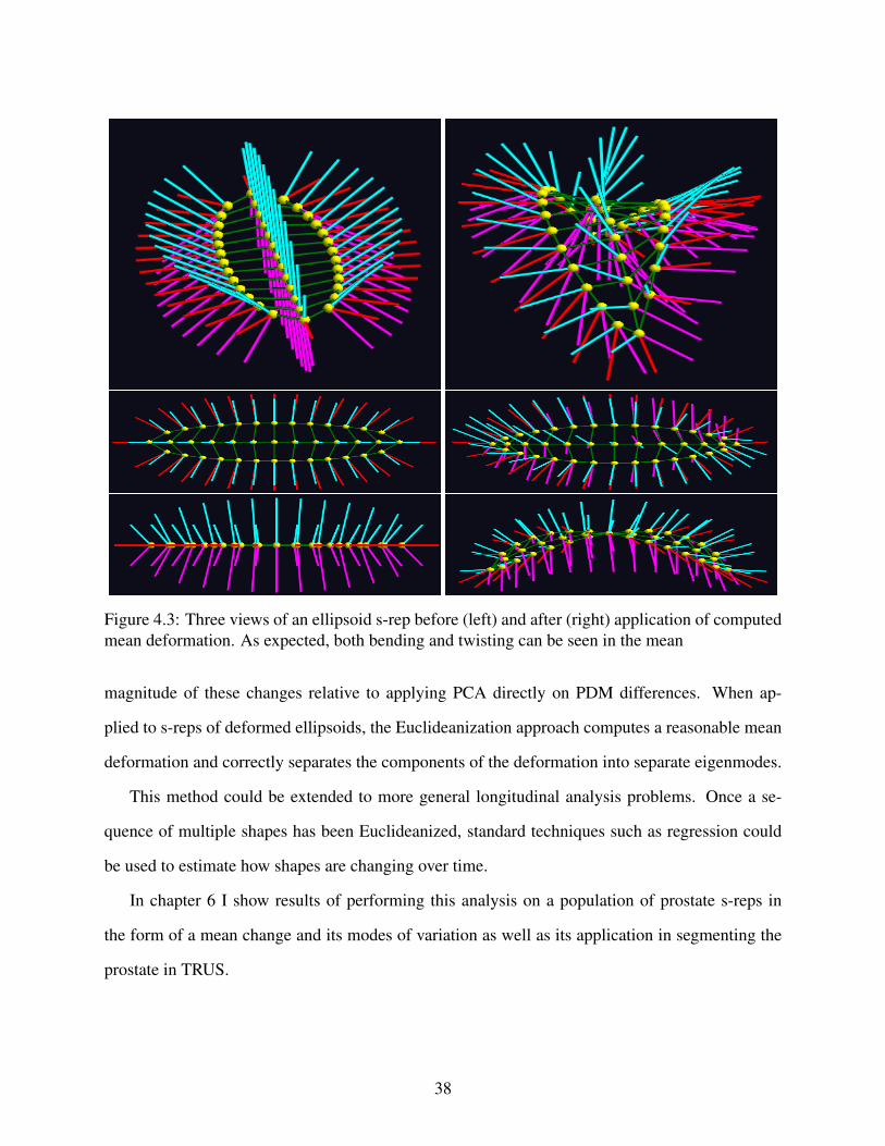
Figure 4.3: Three views of an ellipsoid s-rep before (left) and after (right) application of computedmean deformation. As expected, both bending and twisting can be seen in the mean

magnitude of these changes relative to applying PCA directly on PDM differences. When ap-

plied to s-reps of deformed ellipsoids, the Euclideanization approach computes a reasonable mean

deformation and correctly separates the components of the deformation into separate eigenmodes.

This method could be extended to more general longitudinal analysis problems. Once a se-

quence of multiple shapes has been Euclideanized, standard techniques such as regression could

be used to estimate how shapes are changing over time.

In chapter 6 I show results of performing this analysis on a population of prostate s-reps in

the form of a mean change and its modes of variation as well as its application in segmenting the

prostate in TRUS.

38

Figure 4.4: An ellipsoid deformed -1.5 (left), 0 (middle), and 1.5 (right) standard deviations alongits first (top) and second (bottom) principal components. The first component is dominated by atwisting deformation, while the second is dominated by a bending.

39

5 MODELING TRUS APPEARANCE VIA REGIONAL TEXTURE CLASSIFIERS

5.1 Introduction

As mentioned previously, deformable model segmentation involves deforming an object rep-

resentation so that it better matches the boundary of the desired object in the image. A common

approach is to build a statistical model of the appearance of an object in a particular modality and

use this model in driving the optimization. Building a single, global model for appearance can

be successful when an object’s appearance is relatively uniform or it has strong contrast with the

neighboring anatomy. When these properties do not hold, however, a more fine-grained approach

is required.

Segmentation of the prostate from TRUS is challenging in part because of the difficulties in

discerning the edges of the prostate in ultrasound images. The appearance of both the prostate

and its surrounding anatomy varies widely around its boundary, making the use of a single global

appearance model insufficient and motivating the use of a locally-defined one. In addition, issues

of constrast and noise-like speckle present in the ultrasound images makes direct analysis of ultra-

sound intensity unreliable. Instead, we define appearance in a local fashion using derived texture

features. S-reps provide a convenient method for defining local boundary patches that correspond

across multiple cases. For each patch we take the approach of training a classifier on both texture

and intensity to distinguish between the appearance of voxels just inside the prostate boundary in

that region from those just outside.

From these classifiers we can compute the probability that a voxel in a new image came from

inside the prostate. We then use these probabilities in a new objective function to drive prostate

segmentation. The appearance model itself is the subject of this chapter, while its use in the

segmentation framework is described in chapter 6.5.

40

This overall approach shares several similar characteristics with many of the methods discussed

in section 2.2.6, but it has several important characteristics which none of the other methods fully

capture. Some of the classification-based methods discussed previously perform segmentation

based on the binary decisions output by the classifier, while others turn the classifier outputs into

continuous values using various methods such as application of a sigmoid function to map outputs

to [0, 1]. Instead, I use an application of Bayes’ theorem to further leverage the training data in

order to better understand what the likely distribution of classifier outputs will be when applied to

a new image.

Perhaps the most important characteristic that my method uses for modeling ultrasound ap-

pearance is the strong level of localization used in the training of the appearance classifiers. While

other methods, most notably those of Zhan et al. [40] and Yang et al. [46] use locally trained

classifiers of prostate appearance, they train over many fewer and much larger regions (15 and

6, respectively). This means that their regions often contain many disparate types of tissue and

textures which can lead to poorer classification results, particularly if there is tissue which is rel-

atively similar to prostate texture. In contrast, I am able to leverage the strong correspondences

provided by s-reps to train much more localized texture classifiers, allowing for these classifiers

to be more finely tuned for the specific regions of the image in which they will be applied. Be-

cause s-reps have been shown to produce stronger correspondence than the PDMs typically used

in ASM-based segmentations, these classifiers can be consistently applied on voxels in the correct

regions, minimizing the main drawback of such a scheme.

5.2 Materials

The data used for this work consists of a set of 29 manually segmented 3D TRUS images of

the prostate. We divide the cases into 16 for training and 13 for testing. Each of the prostates from

the training set has been fit with an s-rep using the procedure described in section 2.1.2. Using the

probability distribution computed from the 16 training s-reps, the remaining cases are then fit with

s-reps for use in testing. Each s-rep has 7 rows and 6 colums, resulting in 106 total spokes.

41

5.3 Methodology

In order to build a local appearance model, we must be able to define local regions of the object

boundary which correspond across the training cases. Given a set of such regions, the voxels just

inside the boundary at a region form one class, while the voxels just outside the boundary make up

the other.

For each voxel we have a feature tuple f consisting of some combination of intensity, texture,

or other derived features. For each patch we pool together the inside and outside features from each

training case to form overall inside and outside classes for that patch. From these two classes we

use distance-weighted discrimination (DWD) [64] to compute a separation direction v in feature

space which best separates the appearance of voxels inside and outside the prostate boundary.

Given a separation direction v, we project each training point f onto v yielding a value d. If we

consider the threshold on the separation direction to be at d = 0, the sign of d indicates to which

class f has been assigned, while its magnitude is distance from the separating hyperplane and thus

indicates confidence in this assignment under the assumption that points further from this hyper-

plane are more likely to be correctly classified than those nearer to it. We form two histograms of

d values, one for those voxels from inside the boundary and one for voxels outside the boundary.

These histograms represent the probability distributions p(d|in) and p(d|out), respectively.

Given a new feature tuple, such as one from an image to be segmented, we wish to determine

whether it is more likely that this feature tuple came from inside or outside of the prostate. Assum-

ing we know which regions of the prostate the voxel came from, we can project it along the v for

that region and get its d value. From this d value we wish to know p(in|d). Using Bayes rule we

have

p(in|d) = p(d|in)p(in)p(d|in)p(in) + p(d|out)(1− p(in))

where p(in) is the prior probability of being inside the object and is a parameter that must be set.

If we assume equal probability of coming from inside and outside of the object, this reduces to

42

p(in|d) = p(d|in)p(d|in) + p(d|out)

(5.1)

This allows for the computation of the probability that any particular voxel came from inside the

prostate.

5.4 Application

To build a local appearance model, we must first be able to define local regions around the

prostate boundary which are in correspondence across the training cases. The s-rep fitting pro-

cess ensures that each prostate’s s-rep comes from the same shape space and produces reasonable

correspondence across cases.

Given a set of fit s-reps, we define a local boundary region to be centered at the end of a

spoke and extend halfway to neighboring spokes in each direction, forming a quadrilateral on the

boundary. By moving some distance along the spoke in either direction, we can form inside and

outside regions for the voxels near the boundary.

5.4.1 Ultrasound Appearance Model

As a preprocessing step, each of the TRUS images is unfanned so that the insonation direction,

the direction along which the sound propogates, runs along one of the major axes while the others

represent two axes orthogonal to it. This is done under the observation that much of the texture

information happens either along or orthogonal to the insonation direction. Figure 5.1 shows an

example of the original ultrasound and its unfanned counterpart. In order to decrease the variance

in the ultrasound intensity and to better separate texture and intensity, we run speckle-reducing

anisotropic diffusion [21] on each image. This produces a smoothed intensity image. The differ-

ence between the original image and the smoothed one yields a texture image upon which we can

do texture-based analysis. Figure 5.2 shows an ultrasound image along with its derived intensity

and texture images.

The choice of the feature tuple f that represents each voxel is important to the success of the

43

Figure 5.1: An original, fanned ultrasoundon the left and its defanning on the right.

Figure 5.2: The unfanned ultrasound on theleft, despeckled intensity image in the mid-dle, and texture image on the right.

method. As noted in section 2.2.6, previous work has been done on ultrasound prostate segmenta-

tion making use of either 2D or 3D Gabor filters, and this is what we choose to use here. At each

voxel in the image, we compute 2D Gabor features in 6 orientations, 2 scales (5 and 10 voxels),

and 2 phases in each of the 2 orthogonal planes which include the insonation direction. Combining

these 48 values together with the voxel’s intensity yields a 49-dimensional feature tuple for anal-

ysis. In chapter 6 I show how these feature tuples, after being converted into probabilities, can be

used to drive the image match term of a deformable-model based segmentation.

5.5 Evaluation

Here I evaluate the effectiveness of the appearance model specifically in how well the local

classifiers can classify inside from outside without regard to its ultimate application of segmenta-

tion, which will be discussed in chapter 6.5.

To analyze the effectiveness of the local texture classifiers, I first test to see if there are mean-

ingful differences found between the inside and outside classes in each region. To test this, each

region was subjected to a Direction-Projection-Permutation (DiProPerm) [65] hypothesis test. In

this test, all training features from a given region are projected onto that region’s separation di-

rection. Then, the difference of the mean of the two distributions of d values is computed. The

region’s training points are then randomly relabeled and a new classifier is computed, followed

by a reprojection and recomputation of the mean difference. Iterating this process yields a null

distribution of these mean differences, and we can then check the z-score of the mean difference

for the original labelings.

44

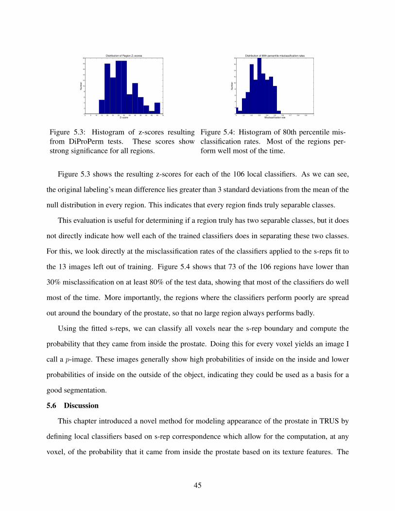
0 5 10 15 20 25 30 35 40 45 50 55 60 65 700

2

4

6

8

10

12

14

16

18

20

Distribution of Region Z−scores

Z−score

Nu

mb

er

Figure 5.3: Histogram of z-scores resultingfrom DiProPerm tests. These scores showstrong significance for all regions.

0 0.1 0.2 0.3 0.4 0.5 0.6 0.7 0.8 0.9 10

2

4

6

8

10

12

14

16

18

Misclassification rate

Nu

mb

er

Distribution of 80th percentile misclassification rates

Figure 5.4: Histogram of 80th percentile mis-classification rates. Most of the regions per-form well most of the time.

Figure 5.3 shows the resulting z-scores for each of the 106 local classifiers. As we can see,

the original labeling’s mean difference lies greater than 3 standard deviations from the mean of the

null distribution in every region. This indicates that every region finds truly separable classes.

This evaluation is useful for determining if a region truly has two separable classes, but it does

not directly indicate how well each of the trained classifiers does in separating these two classes.

For this, we look directly at the misclassification rates of the classifiers applied to the s-reps fit to

the 13 images left out of training. Figure 5.4 shows that 73 of the 106 regions have lower than

30% misclassification on at least 80% of the test data, showing that most of the classifiers do well

most of the time. More importantly, the regions where the classifiers perform poorly are spread

out around the boundary of the prostate, so that no large region always performs badly.

Using the fitted s-reps, we can classify all voxels near the s-rep boundary and compute the

probability that they came from inside the prostate. Doing this for every voxel yields an image I

call a p-image. These images generally show high probabilities of inside on the inside and lower

probabilities of inside on the outside of the object, indicating they could be used as a basis for a

good segmentation.

5.6 Discussion

This chapter introduced a novel method for modeling appearance of the prostate in TRUS by

defining local classifiers based on s-rep correspondence which allow for the computation, at any

voxel, of the probability that it came from inside the prostate based on its texture features. The

45

majority of the local classifiers are able to accurately classify inside from outside in unseen testing

cases and produce reasonable probability images which can be used for segmentation.

One failing of the method in its present form is the use of hard boundaries (i.e., no overlap

between neighbors) on the regions. While the s-rep correspondence behaves adequately in most

cases, the most problematic regions in terms of quality of model tend to be those near the locations

of the prostate boundary where the appearance of the neighboring anatomy changes. The use of

fuzzy region boundaries, such as the considering of neighboring regions texture features when

training the classifiers, could decrease the effect of small correspondence problems and would be

an interesting avenue for future work.

Another place where the method could be improved is the use of the 48 Gabor texture features.

To my knowledge, there is no work that definitively shows that Gabor texture features are better

than other methods for modeling the appearance of the prostate in ultrasound, such as other image-

derived features or physically-based features, though it does appear to be overwhelmingly the most

common approach in the literature. There is also no indication that all 48 features are needed in

every region, and reducing the feature dimension could be useful in reducing computational load

and bringing the method to clinical use.

46

6 SEGMENTATION OF THE PROSTATE FROM TRUS

6.1 Introduction

As discussed in chapter 1.7, there are a number of factors which make prostate segmentation

from 3D TRUS difficult. One of these is the difference in prostate shape caused by the introduc-

tion of the ultrasound transducer, while another is the difficulty in modeling the highly variable

appearance around the prostate boundary in ultrasound images.

In chapter 4.5 I developed a method for estimating probability distributions on deformations

between pairs of shapes. Chapter 5.6 described a method that uses s-reps to define local regions

of the prostate boundary on which classifiers specific to that region’s appearance can be trained,

providing a locally-based appearance model for the prostate boundary in TRUS images. This

chapter describes how these two techniques are used in a deformable model-based segmentation

framework to segment the prostate from TRUS images.

6.2 Materials

As in chapter 5.6, the data used for this work consists of a set of 29 manually segmented 3D

TRUS images of the prostate. I divide the cases into 16 for training and 13 for testing. Each of the

prostates from the training set has been fit with an s-rep using the procedure described in section

2.1.2.

I proceed with the discussion of the segmentation method in this chapter assuming that the

training both of the shape deformation probability distribution from chapter 4.5 and of the local

classifiers described in chapter 5.6 has already been done.

6.3 Segmentation Methodology

This section describes the methodology I use to apply the techniques in chapters 4.5 and 5.6 to

segment the prostate from TRUS images. I perform segmentation using a deformable model-based

47

segmentation framework. The objective function for a deformable segmentation has the general

form

f(x) = P (x) + ωI(x) (6.1)

where x are the parameters of the model’s current state, P measures the log-likelihood of having

the particular model given by x, I measures how well the model matches the image data, and ω is

a parameter used to control the relative weights of the two terms. The objective is to maximize f .

6.3.1 Model Deformation and Probability

In segmenting the prostate from TRUS, a patient’s prostate starts in a normal state and is de-

formed by the TRUS transducer. Chapter 4.5 describes a method for learning a probability distri-

bution on these deformations using a set of pre- and post-deformation prostate s-reps. This method

yields a mean deformation D and a set of shape change eigenvectors v together with their variances

σ2, all in the Euclideanized s-rep space, which together define the shape space I will optimize over.

Given a new case to segment, I assume the existence of a pre-segmented planning-time MRI of

the patient’s prostate with an s-rep fit to it. I apply the learned mean deformation D to the patient’s

initial model MMRI to yield M0US , the initial guess for the patient’s prostate shape in ultrasound.

Because this mean (and its eigenmodes) are learned in Euclideanized rather than ambient space,

the actual computation is

M0US = DE

(E(MMRI) + D

),

where E and DE Euclideanize and de-Euclideanize, respectively, based on the polar system com-

puted via PNS on the group of prostate s-reps.

The parameters x from equation 6.1 of the model deformation are the coefficients for the eigen-

modes of the deformation distribution. For any iteration k of the optimization, the current candidate

model is given by

MkUS = DE

(E(MMRI) + D +

∑i

xki σivi

),

where i ranges over the modes of variation being considered.

48

6.3.2 Probability Images and Image Match

Given a current guess for the patient’s prostate s-rep in the TRUS image, I use the appearance

classifiers described in chapter 5.6 to create a probability image or p-image. These classifiers are

trained on patches of voxels near the boundary, where patches are formed based on neighborhoods

around s-rep sokes. Every voxel within a certain distance of the s-rep boundary has an s-rep spoke

which it is nearest to and so falls within that spoke’s patch. Associated with each voxel is a 49-

dimensional vector of Gabor texture features as described in section 5.4. This feature vector can be

projected onto the DWD separation direction for that patch, giving a value d. From this d value the

probability that that voxel came from inside the prostate, p(in|d), can be computed using equation

5.1. A p-image is created by performing this computation on every voxel within a certain distance

of the s-rep’s boundary. Figure 6.1 shows an example p-image.

Figure 6.1: An example p-image of a prostate. High intensities reflect high p(in|d) for that voxel.

Intuitively, a good segmentation should have voxels with high average p(in|d) inside the candi-

date boundary and low average p(in|d) values outside it. I define the match value I from equation

49

6.1, for an object with k regions, as

I =∑

Ωi=1...k

[(ρini − ρouti

)− |ρini + ρouti − 1|

]. (6.2)

where ρink and ρoutk are the average p(in|d) values for the regions inside and outside, respectively,

the kth patch. The first term encourages large differences in the means for the inside and outside

patches (ρin = 0.7 and ρout = 0.2 is better than ρin = 0.6 and ρout = 0.35) while the second

encourages the midpoint of ρink and ρoutk to be near 0.5 ( ρin = 0.7 and ρout = 0.3 is better than

ρin = 0.9 and ρout = 0.5 even though the separation is the same.)

6.3.3 Optimization

The optimization of equation 6.1 proceeds via a standard conjugate gradient optimization of

x, deforming the prostate to more closely match the current p-image. After each iteration, the

p-image is recomputed using the new candidate model.

6.4 Results

6.4.1 Estimation of Prostate Deformation Distribution

The mean and modes of variation of the prostate’s deformation from planning-time MRI to

biopsy-time TRUS were computed from the 16 training cases using the method described in chap-

ter 4. The computed mean deformation shows the denting characteristic of the effect of the TRUS

transducer, and the eigenmodes show various other changes in the TRUS dent and thus the shape of

the prostate. Figure 6.2 shows an example of the computed mean deformation applied to a single

prostate case. Videos of deformation along the first few eigenmodes are available online [66]. For

segmentation, I optimize over the first 10 eigenmodes, which capture 93% of the total variance.

6.4.2 Segmentation

The shape space described in section 6.4.1 can be used to segment the prostate in TRUS. In

each of the 13 test cases, an initial prostate is obtained by applying the mean deformation to an

s-rep fit to that patients pre-segmented planning-time MRI, serving as the initial guess for that

patient’s deformed prostate shape. This s-rep is then manually aligned into the TRUS image,

50

Figure 6.2: A prostate segmented from planning-time MRI (left) and this prostate with the meandeformation applied (right). Notice the large dent in the post-deformation model. This is similarto the typical dents caused by the TRUS transducer.

although an automatic method, such as one which matches the dent in the prostate to the location

of the TRUS transducer, could be used. From this initial aligned s-rep, a p-image is calculated,

and the s-rep is deformed along the eigenmodes of the deformation distribution to better match the

image. From this new s-rep a new p-image is computed, and the process is iterated. I evaluate the

quality of these segmentations based on two metrics: Dice Similarity Coefficient (DSC) and mean

absolute distance (MAD) between my segmentation and a ground truth manual segmentation. The

computations are performed via MeshValmet [67].

This procedure yields segmentations with an average DSC of 0.783 and MAD of 2.76 compared

to ground truth manual segmentations. While these results are not unencouraging, this global

optimization clearly does not do well enough to be clinically useful on its own. The need for

further refinement is typical of the case when a global optimization over a limited number of

eigenmodes is performed.

6.4.3 Refinement

This segmentation via global deformation of the s-rep comes as close as it can to match the

p-image by staying within the shape space, but some areas of the prostate will be more well-

segmented than others. To address this issue, I include a refinement step to the segmentation

following the global optimziation. In this stage, spokes in regions where the classifiers are known

to perform well are either lengthened or shortened to better match the p-image (note that, because

51

there are no angular changes to spokes, the s-rep region a voxel falls in does not change at this

stage). The voxels near the s-rep boundary at each such spoke are then examined to see how well

the segmentation is doing in that region.

In regions where there are high probabilties inside and low probabilities outside, the spoke

stays as is. In regions where there are all high probabilties, the spoke is gradually lengthened until

it finds an outside region with low probabilities, and a similar approach is taken for spokes which

have low probabilities everywhere. Spokes are constrained to not gain or lose more than 25% of

their original lengths. In order to maintain smooth s-rep boundaries, the change in a spoke’s length

is propogated to its neighbors, falling off quickly so as to only change nearby spokes.

Using this approach, the segmentations described in section 6.4.2 can be improved to have an

average DSC of 0.903 and MAD of 1.4, both of which are competitive with state of the art. A

comparison to the accuracies reported for other methods is given in table 6.3. These methods each

require a small amount (typically the marking of a few points) of user interaction and were tested

on similar sized datasets of 25-30 prostates.

Method Year DSC MADTutar[45] 2006 .835 1.3

Garnier[32] 2011 .864 0.8Mahdavi[20] 2011 - 0.7

Qiu[23] 2013 .932 1.1Proposed 2015 .903 1.4

Figure 6.3: Results of the proposed method compared with other recently published methods.

This refinement approach is simply an initial attempt to refine the segmentations and as such is

not yet fully developed or claimed as a contribution of this dissertation. Nevertheless, it shows that

the combination of the shape space developed in chapter 4 and the appearance model developed in

chapter 5 form a promising basis for performing good segmentations.

6.5 Discussion

The segmentation method presented in this chapters shows an ability to accurately segment the

prostate from TRUS by combining the appearance model proposed in chapter 5 with the method

52

for estimating an individual’s prostate shape from chapter 4. The results obtained by a simple

optimization over the shape space show promise, while a simple refinement method produces seg-

mentations which are competitive with other recently published methods.

It is interesting to compare these results to a previous attempt, with the most notable difference

being that the old attempt used a different method for estimating prostate shape. Instead of the

method described in chapter 4, it used a different s-rep-based metric (spoke direction changes as

rotations, radius changes as scalings, and hub position changes as regular Euclidean differences),

applied each computed deformation to a single reference case, and then computed statistics on

these deformed references. To apply to a new case, the reference case would be subtracted from

the mean of the deformed cases and the resulting difference would be applied to the new case.

In this previous try, the initial segmentation was much worse (0.718 vs 0.783 DSC) while the

final segmentations (0.893/1.7 vs 0.903/1.4) are closer. This shows that the proposed method for

estimating probability distributions on shape differences is superior to the previously used method,

but that both segmentations seem to be reaching the limit of the current appearance model’s ability

to produce better p-images.

There are two factors currently limiting the usefulness of the appearance model’s application

to the segmentation problem: the use of hard patch boundaries and the density of the base s-rep

used. The regions where the segmentation performs worse tend to be regions where the appearance

of the tissue outside of the prostate changes, which would be alleviated by moving to fuzzy patch

boundaries so that the appearance of neighboring patches would be considered when training each

classifier. Increasing the s-rep density would allow for more closely matching the s-rep boundary

by giving the s-rep the ability to have more finely grained local changes, but this would increase

the previously described problem if it was not also paired with fuzzy patch boundaries.

53

7 CONCLUSIONS & DISCUSSION

This dissertation presented a method for segmentation of the prostate from TRUS during biopsy

using a novel statistical model for how the TRUS transducer affects the prostate shape as well as

novel learned regional classifiers on prostate appearance. S-reps provide a rich object representa-

tion well suited to both of these tasks. I described a method for learning a probability distribution

on how an individual’s prostate is deformed by the TRUS during image-guided biopsy and pro-

vided a means for leveraging the inherent localization ability of s-reps to train local classifiers for

corresponding regions across a set of patients. Chapter 6.5 used these methods in a deformable

segmentation framework to produce prostate segmentations which are competitive with the latest

methods from the literature.

The contributions of this dissertation are as follows:

1. The development and implementation of a method for producing smooth continuous skeletal

models from discrete s-reps. I used the extension to skeletal models of the mathematics of

medial models to create a geometrically-based interpolation of discrete s-reps.

2. The development of a method using s-reps for computing probability distributions of how

a shape changes from one state to another. Using representations of pairs of before/after

objects, I use Euclideanization to transform the representations into a space where Euclidean

statistical methods can be used to analyze the difference between before and after objects,

avoiding the pain that comes with dealing with shape representations on the curved spaces

in which they actually live.

3. The use of s-reps as a basis for the training of localized classifiers of object intensity and

texture.

54

4. The computation of the probability that a new voxel from a particular region came from

inside the prostate.

5. The combination of the previously mentioned techniques into a deformable segmentation

framework to segment the prostate from biopsy-time TRUS images.

From these contributions I derive the following thesis:

Thesis: Segmentation of an object deformed from a base state in a systematic way with appear-

ance that varies around its boundary benefits from combining the following two approaches:

1. Statistical analysis of the object deformation by a method suited for analysis in curved spaces

2. Regionally trained appearance models to distinguish voxels inside and outside of the object’s

boundary in a classification-based approach.

Instead of the more typical boundary-based approach, continuously interpolated skeletal models

form a strong basis for the training of statistics of object deformation as well as the creation of

object-relative regions on which to train appearance models.

7.1 Discussion and Future Work

7.1.1 S-reps and Fitting

The work in this dissertation as well as various related works [10, 5, 6] in the past few years

have shown that s-reps are a powerful representation for modeling object shape. One of the major

hurdles to s-reps gaining more widespread use is the various difficulties associated with using the

related software. Steps have been taken recently to reduce these problems, but there is much work

still to be done.

A major barrier to beginning to use s-reps has been the process used to fit s-reps to binary im-

ages. The fitting process in Pablo is driven through the use of plain-text configuration files, which

are lists of various penalty terms which are used to weight various parts of the fitting optimization’s

objective function. The best values for these weights depend on a number of things, including the

55

particular object, the base s-rep grid size, and which of the various properties are desirable for that

model to have.

Typically, creating a good configuration file consists of modifying one or more weights, re-

running the fit, checking the result visually, changing some weights to correct some problem, and

iterating. This is a tedious process that can result in a configuration file that is overly tuned for the

specific case or cases used in the creation, so sometimes the file must be retuned after a population-

wide fit is done.

The fitting process has been somewhat marginalized by the development of the thin plate spline

(TPS)-based initialization method used to fit the s-reps described in chapter 4.5, which in many

applications can replace the old initial fitting step called the atom stage, which greatly reduces the

amount of work needed to create an initial set of s-reps. This TPS-based method requires a set of

initial correspondences for the template model as well as each individual case. Currently, these

correspondences can come from any source that produces corresponding PDMs. Early work used

SPHARM-PDM [7] to generate these correspondences, but this method can produce unreliable

correspondences when there is an ambiguity in the fitting of an ellipsoid to the object, such as

when there is strong rotational symmetry. For this reason, I instead used the method of thin-shell

demons [9] to register PDMs representing two objects and used the correspondence implied by

this registration to fuel the TPS. While this method worked well for the prostates, it is unclear if it

would be suitable for objects which had larger expected deformations.

7.1.2 Interpolation

The s-rep interpolation method presented here has been quite successful in producing qualita-

tively (and quantitatively in those objects where a ground truth is known) good s-reps. The method

tends to produce high quality interpolation except in those regions where the spokes change direc-

tion rapidly, most notably at the corners of the s-rep grid, a problem which could be alleviated by

moving away from the rectangular grid as the basis for s-rep representation. From what I have been

able to tell, this is caused largely by the use of Bezier curves in the interpolation, which can curve

56

more wildly than is desired in such cases. Using a different set of basis functions could improve

the accuracy of the interpolation in these regions.

This interpolation is highly parallelizable on a quad-by-quad basis, and because the s-reps are

reinterpolated frequently in the core of many of the presented algorithms, it is necessary to leverage

as much parallelism as possible. Currently, the averaging process described in section 3.7 is done

in parallel for each spoke, but there is no spoke-level or quad-level parallelism as of yet.

Some work has been done on finding a closed-form solution for the interpolation which would

allow for much more efficient computation, but it has not yet been carried to a usable state.

This interpolation is extendable to quasitubular s-rep models, though this work has not yet been

performed.

7.1.3 Statistics on Shape Differences

The presented method for computing probability distributions of shape deformations proved

powerful for accurately recovering underlying deformations in synthetic ellipsoid data, both for

PDM and s-rep representations. It also showed the ability to represent the deformation caused

by the TRUS transducer to the shape of the prostate and provide a basis for an accurate prostate

segmentation. The method currently relies on a pooled set of before and after shapes to compute the

PNS polar systems that allow for Euclideanization, but it is unclear whether this technique would

be applicable if the underlying deformations were larger. In cases where the before and after shapes

are too far separated, the PNS computation on two separate groups can produce results which do

not accurately represent either.

I believe that this method is applicable in situations beyond simply estimating probability dis-

tributions for use in segmentation. Future work could include using the differences of the Eu-

clideanized shapes in other tasks, such as categorizing the progression of an anatomical object as

either normal or pathological.

57

7.1.4 Appearance Model

The presented appearance model is able to accurately classify the texture of voxels inside the

prostate from those outside the prostate in a large majority of the prostate boundary, providing a

basis for an accurate segmentation. The appearance model could potentially increase performance

even further with the use of features other than 2D Gabor features for modeling texture. In particu-

lar, the exploration of features which take into account the physics of the TRUS image acquisition

could be powerful. It would also be desirable to explore using a reduced set of particularly infor-

mative features to ease computational load.

The prostate boundary patches with low classification performance tend to come from the re-

gions surrounding areas of the boundary where the appearance changes. This is caused by training

linear classifiers for data which may have more than two clusters, such as the inside appearances

vs 2 or 3 different classes of outside appearances, some of which may be close to the inside ap-

pearances and thus produce a higher rate of misclassifications. This problem could potentially be

solved using a non-linear kernel for the classifier.

There is nothing about this appearance model that is specific to the task of prostate segmenta-

tion from ultrasound. While the specific features used for classification will likely be different for

other objects or modalities, the underlying strategy of using s-reps to heavily localize the object

boundary, train classifiers to tell inside from outside appearance, and use the learned distribution

of each region’s features during classification to produce probabilities, could be adapted to many

different scenarios.

7.1.5 Segmentation

The segmentation method presented shows promising results, able to produce segmentations

whose accuracy is competitive with other recently published TRUS prostate segmentation algo-

rithms. However, there are several potential areas of improvement.

One problem, related to a problem mentioned for the appearance model, is that because the

candidate segmentations are only guesses for the actual shape of the model, the s-reps regions

58

are not precisely in the prostate regions they are during training. Because of the hard boundary

constraints between regions, a classifier may be seeing appearance it has never seen before and

thus perform poorly. However, it is likely that, if the initial alignment is good, each spoke of

the s-rep is near its correct region. By changing the hard boundary constraints in the training

to fuzzy ones, so that the appearance of the regions neighboring region k are taken into account

when training region k, it is less likely that the classifier is seeing something new so the expected

accuracy should increase.

While the focus of this dissertation was on the methodological pieces which make up the seg-

mentation algorithm rather than the segmentation itself, an initial try at a method for refining the

initial segmentation is presented. This method shows good results, but further work is needed to

address some of its drawbacks. For shapes which are very different in some region than the initial

guess, the capture distance for the refinement step can be difficult to tune. Accurately finding the

boundary means having some inside and some outside voxels in a region so that the boundary

between the two shows up in the p-image. A naive scheme where, if the region is seeing only

high p(in) values it looks farther out and vice versa, was applied, but more sophisticated methods,

such as local histogram analysis or machine learning approaches to learn where to search for the

boundary, could make this process both faster and more accurate. There are also still issues of

the refinement of one spoke changing the position of neighboring spokes, which can pull those

spokes to less desirable places in their own regions. There is a difficult balance to strike between

accuracy of one spoke and its effect on its neighbors, though moving to using fuzzy regions for the

appearance model could alleviate this somewhat.

A major hurdle in making this segmentation method clinically usable is the speed. Currently,

the time taken to perform a single segmentation is on the order of an hour, whereas it would need

to run in a few seconds at most to be used during a biopsy procedure. There are, however, several

areas where this speed could be improved. As mentioned previously, the interpolation method

could be greatly sped up by taking advantage of the highly parallel nature of the computation.

59

Another area where the speed could be improved is in the computation of the texture features,

which currently requires 48 separate computations at every voxel in the image. Because the values

computed for each voxel are independent of the values computed for neighboring voxels, this

process is also highly parallelizable. Choosing a smaller set of more representative features would

also make this computation more efficient. Finally, only computing them in the regions of the

image where the prostate is most likely to be (or alternatively only in the areas currently being

considered by the candidate segmentation) may also be useful, though the TRUS images do not

typically capture anatomy very far from the prostate.

7.1.6 Conclusions

While this chapter has focused mainly on the drawbacks and future improvements to be made to

the various pieces of methodology presented here, the prostate segmentation method as it currently

stands seems sound and has been able to produce quality results. While here the pieces of the

method are applied to a prostate segmentation, none of these methods are specific to this ultimate

goal and could be applied, either individually or collectively, to other problems. In particular, the

method for producing statistics on shape differences could be applied to any task where the change

in a shape from one time to another is of interest and the appearance model could be applied in any

case with an object representation that supports localization. It is my hope that these methods will

be applied to other problems in the future.

60

REFERENCES

[1] A. C. Society, “Cancer Facts & Figures 2016,” American Cancer Society, 2016.

[2] J. Bax, D. Cool, L. Gardi, K. Knight, D. Smith, J. Montreuil, S. Sherebrin, C. Romagnoli, andA. Fenster, “Mechanically assisted 3D ultrasound guided prostate biopsy system. ,” vol. 35,no. 12, pp. 5397–5410, 2008.

[3] T. F. Cootes, C. J. Taylor, D. H. Cooper, and J. Graham, “Active shape models-their trainingand application,” Computer vision and image understanding, vol. 61, no. 1, pp. 38–59, 1995.

[4] S. M. Pizer, S. Jung, D. Goswami, J. Vicory, X. Zhao, R. Chaudhuri, J. N. Damon, S. Hucke-mann, and J. Marron, “Nested sphere statistics of skeletal models,” in Innovations for ShapeAnalysis: Models and Algorithms (M. Breuss, A. Bruckstein, and P. Maragos, eds.), pp. 93–113, Springer, 2013.

[5] J. Hong, J. Vicory, J. Schulz, M. Styner, J. Marron, and S. M. Pizer, “Non-euclidean classifi-cation of medically imaged objects via s-reps,” Medical Image Analysis, vol. 31, pp. 37–45,2016.

[6] L. Tu, J. Vicory, S. Elhabian, B. Paniagua, J. C. Prieto, R. Whitaker, M. Styner, and S. M.Pizer, “Entropy-based correspondence improvement of interpolated skeletal models,” Com-puter Vision and Image Understanding, 2016.

[7] M. Styner, I. Oguz, S. Xu, C. Brechbuhler, D. Pantazis, J. J. Levitt, M. E. Shenton, andG. Gerig, “Framework for the statistical shape analysis of brain structures using spharm-pdm,” The insight journal, no. 1071, p. 242, 2006.

[8] J. Cates, P. T. Fletcher, M. Styner, M. Shenton, and R. Whitaker, “Shape modeling and anal-ysis with entropy-based particle systems,” in Information Processing in Medical Imaging,pp. 333–345, Springer, 2007.

[9] Q. Zhao, T. Price, S. Pizer, M. Niethammer, R. Alterovitz, and J. Rosenman, “Surface regis-tration in the presence of missing patches and topology change,” in Proceedings of the 19thConference on Medical Image Understanding and Analysis, 2015.

[10] J. Schulz, S. M. Pizer, J. S. Marron, and F. Godtliebsen, “Non-linear hypothesis testing of ge-ometric object properties of shapes applied to hippocampi,” Journal of Mathematical Imagingand Vision, vol. 54, no. 1, pp. 15–34, 2016.

[11] J. Damon and J. S. Marron, “Backwards principal component analysis and principal nestedrelations,” Journal of Mathematical Imaging and Vision, vol. 50, no. 1-2, pp. 107–114, 2014.

[12] P. Fletcher, C. Lu, S. Pizer, and S. Joshi, “Principal Geodesic Analysis for the Study of Non-linear Statistics of Shape,” IEEE Transactions on Medical Imaging, vol. 23, no. 8, pp. 995–1005, 2004.

[13] S. Huckemann, T. Hotz, and A. Munk, “Intrinsic shape analysis: Geodesic pca for riemannianmanifolds modulo isometric lie group actions,” Statistica Sinica, pp. 1–58, 2010.

61

[14] D. G. Kendall, “Shape manifolds, procrustean metrics, and complex projective spaces,” Bul-letin of the London Mathematical Society, vol. 16, no. 2, pp. 81–121, 1984.

[15] S. Jung, I. L. Dryden, and J. Marron, “Analysis of Principal Nested Spheres,” Biometrika,pp. 1–27, 2010.

[16] S. Ghose, A. Oliver, R. Mart, X. Llad, J. C. Vilanova, J. Freixenet, J. Mitra, D. Sidib,and F. Meriaudeau, “A survey of prostate segmentation methodologies in ultrasound, mag-netic resonance and computed tomography images,” Computer Methods and Programs inBiomedicine, vol. 108, no. 1, pp. 262 – 287, 2012.

[17] J. A. Noble and D. Boukerroui, “Ultrasound image segmentation: a survey,” Medical Imag-ing, IEEE Transactions on, vol. 25, no. 8, pp. 987–1010, 2006.

[18] R. Aarnink, S. D. Pathak, J. J. de la Rosette, F. M. Debruyne, Y. Kim, and H. Wijkstra, “Edgedetection in prostatic ultrasound images using integrated edge maps,” Ultrasonics, vol. 36,no. 1, pp. 635–642, 1998.

[19] S. D. Pathak, D. Haynor, and Y. Kim, “Edge-guided boundary delineation in prostate ultra-sound images,” Medical Imaging, IEEE Transactions on, vol. 19, no. 12, pp. 1211–1219,2000.

[20] S. S. Mahdavi, M. Moradi, X. Wen, W. J. Morris, and S. E. Salcudean, “Evaluation of visual-ization of the prostate gland in vibro-elastography images,” Medical image analysis, vol. 15,no. 4, pp. 589–600, 2011.

[21] Y. Yu and S. T. Acton, “Speckle Reducing Anisotropic Diffusion,” IEEE Transactions onImage Processing, vol. 11, no. 11, pp. 1260–1271, 2002.

[22] M. Zouqi and J. Samarabandu, “Prostate segmentation from 2-d ultrasound images usinggraph cuts and domain knowledge,” in Computer and Robot Vision, 2008. CRV’08. CanadianConference on, pp. 359–362, IEEE, 2008.

[23] W. Qiu, J. Yuan, E. Ukwatta, Y. Sun, M. Rajchl, and A. Fenster, “Prostate segmentation: Anefficient convex optimization approach with axial symmetry using 3-d trus and mr images,”Medical Imaging, IEEE Transactions on, vol. 33, no. 4, pp. 947–960, 2014.

[24] A. Zaim, “Automatic segmentation of the prostate from ultrasound data using feature-basedself organizing map,” in Image Analysis, pp. 1259–1265, Springer, 2005.

[25] A. Zaim, T. Yi, and R. Keck, “Feature-based classification of prostate ultrasound imagesusing multiwavelet and kernel support vector machines,” in Neural Networks, 2007. IJCNN2007. International Joint Conference on, pp. 278–281, IEEE, 2007.

[26] S. Mohamed, A. Youssef, E. El-Saadany, and M. Salama, “Prostate tissue characterizationusing trus image spectral features,” in Image Analysis and Recognition (A. Campilho andM. Kamel, eds.), vol. 4142 of Lecture Notes in Computer Science, pp. 589–601, SpringerBerlin Heidelberg, 2006.

62

[27] W. D. Richard and C. G. Keen, “Automated texture-based segmentation of ultrasound imagesof the prostate,” Computerized Medical Imaging and Graphics, vol. 20, no. 3, pp. 131–140,1996.

[28] M. Kass, A. Witkin, and D. Terzopoulos, “Snakes: Active contour models,” Internationaljournal of computer vision, vol. 1, no. 4, pp. 321–331, 1988.

[29] A. Jendoubi, J. Zeng, and M. F. Chouikha, “Segmentation of prostate ultrasound imagesusing an improved snakes model,” in Signal Processing, 2004. Proceedings. ICSP’04. 20047th International Conference on, vol. 3, pp. 2568–2571, IEEE, 2004.

[30] C. Knoll, M. Alcaniz, V. Grau, C. Monserrat, and M. C. Juan, “Outlining of the prostate usingsnakes with shape restrictions based on the wavelet transform (doctoral thesis: Dissertation),”Pattern Recognition, vol. 32, no. 10, pp. 1767–1781, 1999.

[31] A. Zaim and J. Jankun, “An energy-based segmentation of prostate from ultrasouind imagesusing dot-pattern select cells,” in Acoustics, Speech and Signal Processing, 2007. ICASSP2007. IEEE International Conference on, vol. 1, pp. I–297, IEEE, 2007.

[32] C. Garnier, J.-J. Bellanger, K. Wu, H. Shu, N. Costet, R. Mathieu, R. De Crevoisier, and J.-L.Coatrieux, “Prostate segmentation in hifu therapy,” Medical Imaging, IEEE Transactions on,vol. 30, no. 3, pp. 792–803, 2011.

[33] S. Lobregt and M. A. Viergever, “A discrete dynamic contour model,” IEEE transactions onmedical imaging, vol. 14, no. 1, pp. 12–24, 1995.

[34] K. Li, X. Wu, D. Z. Chen, and M. Sonka, “Efficient optimal surface detection: theory, im-plementation, and experimental validation,” in Proceedings of SPIE, vol. 5370, pp. 620–627,2004.

[35] H. M. Ladak, F. Mao, Y. Wang, D. B. D. B. Downey, D. Steinman, and A. Fenster, “Prostatesegmentation from 2d ultrasound images,” in Engineering in Medicine and Biology Soci-ety, 2000. Proceedings of the 22nd Annual International Conference of the IEEE, vol. 4,pp. 3188–3191, IEEE, 2000.

[36] M. Ding, C. Chen, Y. Wang, I. Gyacskov, and A. Fenster, “Prostate segmentation in 3d usimages using the cardinal-spline-based discrete dynamic contour,” in Medical Imaging 2003,pp. 69–76, International Society for Optics and Photonics, 2003.

[37] D. Shen, Y. Zhan, and C. Davatzikos, “Segmentation of prostate boundaries from ultra-sound images using statistical shape model,” IEEE Transactions on Medical Imaging, vol. 22,pp. 539–551, 2003.

[38] N. Betrouni, M. Vermandel, D. Pasquier, S. Maouche, and J. Rousseau, “Segmentation ofabdominal ultrasound images of the prostate using a priori information and an adapted noisefilter,” Computerized Medical Imaging and Grahpics, vol. 29, no. 1, pp. 43–51, 2005.

63

[39] Y. Zhan and D. Shen, “Automated segmentation of 3d us prostate images using statisti-cal texture-based matching method,” in Medical Image Computing and Computer-AssistedIntervention-MICCAI 2003, pp. 688–696, Springer, 2003.

[40] Y. Zhan and D. Shen, “Deformable Segmentation of 3-D Ultrasound Prostate Images UsingStatistical Texture Matching Method,” IEEE Transactions on Medical Imaging, vol. 25, no. 3,pp. 256–272, 2006.

[41] F. A. Cosıo, “Automatic initialization of an active shape model of the prostate,” MedicalImage Analysis, vol. 12, no. 4, pp. 469–483, 2008.

[42] T. Cootes, G. Edwards, and C. Taylor, “Active Appearance Models,” in Proc. European Con-ference on Computer Vision, 1998.

[43] R. Medina, A. Bravo, P. Windyga, J. Toro, P. Yan, and G. Onik, “A 2d active appearancemodel for prostate segmentation in ultrasound images,” in 27th Annual international confer-ence of the IEEE engineering in medicine and biology society, pp. 3363–3366, 2005.

[44] S. Ghose, A. Oliver, R. Martı, X. Llado, J. Freixenet, J. C. Vilanova, and F. Meriaudeau,“Texture guided active appearance model propagation for prostate segmentation,” in ProstateCancer Imaging. Computer-Aided Diagnosis, Prognosis, and Intervention, pp. 111–120,Springer, 2010.

[45] I. B. Tutar, S. D. Pathak, L. Gong, P. S. Cho, K. Wallner, and Y. Kim, “Semiautomatic 3-dprostate segmentation from trus images using spherical harmonics,” Medical Imaging, IEEETransactions on, vol. 25, no. 12, pp. 1645–1654, 2006.

[46] X. Yang, D. Schuster, V. Master, P. Nieh, A. Fenster, and B. Fei, “Automatic 3d segmentationof ultrasound images using atlas registration and statistical texture prior,” in SPIE MedicalImaging, pp. 796432–796432, International Society for Optics and Photonics, 2011.

[47] S. Martin, J. Troccaz, and V. Daanen, “Automated segmentation of the prostate in 3d mrimages using a probabilistic atlas and a spatially constrained deformable model,” Medicalphysics, vol. 37, no. 4, pp. 1579–1590, 2010.

[48] Y. Gao, Y. Zhan, and D. Shen, “Incremental learning with selective memory (ilsm): Towardsfast prostate localization for image guided radiotherapy,” IEEE transactions on medical imag-ing, vol. 33, no. 2, pp. 518–534, 2014.

[49] J. R. C. Crouch, Medial techniques for automating finite element analysis. PhD thesis, Cite-seer, 2003.

[50] Q. Han, S. M. Pizer, and J. N. Damon, “Interpolation in discrete single figure medial objects,”in Computer Vision and Pattern Recognition Workshop, 2006. CVPRW’06. Conference on,pp. 85–85, IEEE, 2006.

64

[51] J. Damon, “Smoothness and Geometry of Boundaries Associated to Skeletal Structions I:Sufficient Conditions for Smoothness,” Annales de Institut Fourier, vol. 14, no. 6, pp. 1941–1985, 2003.

[52] K. Siddiqi and S. M. Pizer, Medial representations: mathematics, algorithms and applica-tions, vol. 37. Springer, 2008.

[53] J. N. Damon. personal correspondence, 2014.

[54] K. Shoemake, “Animating rotation with quaternion curves,” in ACM SIGGRAPH computergraphics, vol. 19, pp. 245–254, ACM, 1985.

[55] K. Shoemake, “Quaternion calculus and fast animation, computer animation: 3-d motionspecification and control,” Siggraph, 1987.

[56] E. B. Dam, M. Koch, and M. Lillholm, Quaternions, interpolation and animation. DatalogiskInstitut, Københavns Universitet, 1998.

[57] S. M. Pizer, To compute numerically: Concepts and strategies (Little, Brown computer sys-tems series). Little, Brown & Co. Inc., 1983.

[58] I. L. Dryden and K. V. Mardia, Statistical shape analysis, vol. 4. J. Wiley Chichester, 1998.

[59] J. G. Csernansky, L. Wang, S. C. Joshi, J. T. Ratnanather, and M. I. Miller, “Computationalanatomy and neuropsychiatric disease: probabilistic assessment of variation and statisticalinference of group difference, hemispheric asymmetry, and time-dependent change,” Neu-roimage, vol. 23, pp. S56–S68, 2004.

[60] L. Wang, J. S. Swank, I. E. Glick, M. H. Gado, M. I. Miller, J. C. Morris, and J. G. Cser-nansky, “Changes in hippocampal volume and shape across time distinguish dementia of thealzheimer type from healthy aging,” Neuroimage, vol. 20, no. 2, pp. 667–682, 2003.

[61] M. Vaillant, M. I. Miller, L. Younes, and A. Trouve, “Statistics on diffeomorphisms via tan-gent space representations,” NeuroImage, vol. 23, pp. S161–S169, 2004.

[62] L. Wang, F. Beg, T. Ratnanather, C. Ceritoglu, L. Younes, J. C. Morris, J. G. Csernansky, andM. I. Miller, “Large deformation diffeomorphism and momentum based hippocampal shapediscrimination in dementia of the alzheimer type,” Medical Imaging, IEEE Transactions on,vol. 26, no. 4, pp. 462–470, 2007.

[63] S. Durrleman, X. Pennec, A. Trouve, J. Braga, G. Gerig, and N. Ayache, “Toward a com-prehensive framework for the spatiotemporal statistical analysis of longitudinal shape data,”International journal of computer vision, vol. 103, no. 1, pp. 22–59, 2013.

[64] J. Marron, M. Todd, and J. Ahn, “Distance Weighted Discrimination,” Journal of the Ameri-can Statistical Association, vol. 102, pp. 1267–1271, 2007.

65

[65] S. Wei, C. Lee, L. Wichers, and J. Marron, “Direction-projection-permutation for high di-mensional hypothesis tests,” Journal of Computational and Graphical Statistics, no. just-accepted, 2015.

[66] “Prostate eigenmode videos.” https://dl.dropboxusercontent.com/u/12881668/prostatemodes.html.

[67] “Meshvalmet.” https://www.nitrc.org/projects/meshvalmet/.

66