Jess Benhabib - Columbia Universityss3501/research/avoiding.pdfJess Benhabib New York University ... Wieland, and Williams (1999) use a nonoptimizing, rational expecta-tions model

535

[Journal of Political Economy, 2002, vol. 110, no. 3]� 2002 by The University of Chicago. All rights reserved. 0022-3808/2002/11003-0002$10.00

Avoiding Liquidity Traps

Jess BenhabibNew York University

Stephanie Schmitt-GroheRutgers University and Centre for Economic Policy Research

Martın UribeUniversity of Pennsylvania

Once the zero bound on nominal interest rates is taken into account,Taylor-type interest rate feedback rules give rise to unintended self-fulfilling decelerating inflation paths and aggregate fluctuationsdriven by arbitrary revisions in expectations. These undesirable equi-libria exhibit the essential features of liquidity traps since monetarypolicy is ineffective in bringing about the government’s goals regard-ing the stability of output and prices. This paper proposes severalfiscal and monetary policies that preserve the appealing features ofTaylor rules, such as local uniqueness of equilibrium near the inflationtarget, and at the same time rule out the deflationary expectationsthat can lead an economy into a liquidity trap.

We wish to thank Mike Woodford for many very helpful comments and suggestions onBenhabib, Schmitt-Grohe, and Uribe (2001b) at the 1999 NBER Summer Institute, whichled to the writing of this paper and on which our analysis is based. We are also gratefulto John Cochrane, the editor, and three anonymous referees for very helpful commentsand suggestions. We acknowledge technical assistance from the C. V. Starr Center ofApplied Economics at New York University.

536 journal of political economy

I. Introduction

In recent years, there has been a revival of empirical and theoreticalresearch aimed at understanding the macroeconomic consequences ofmonetary policy regimes that take the form of interest rate feedbackrules. One driving force of this renewed interest can be found in em-pirical studies showing that in the past two decades monetary policy inthe United States is well described as following such a rule. In particular,an influential paper by Taylor (1993) characterizes the Federal Reserveas following a simple rule whereby the federal funds rate is set as alinear function of inflation and the output gap with coefficients of 1.5and 0.5, respectively. Taylor emphasizes the stabilizing role of an infla-tion coefficient greater than unity, which loosely speaking implies thatthe central bank raises real interest rates in response to increases in therate of inflation. After his seminal paper, interest rate feedback ruleswith this feature have become known as Taylor rules. Taylor rules havealso been shown to represent an adequate description of monetary pol-icy in other industrialized economies (see, e.g., Clarida, Galı, and Gertler1998).

At the same time, a growing body of theoretical work has argued thatTaylor rules contribute to macroeconomic stability. Researchers havearrived at this conclusion following different routes. For example, Levin,Wieland, and Williams (1999) use a nonoptimizing, rational expecta-tions model and find that a Taylor rule is the optimal interest ratefeedback rule in the sense that it minimizes a quadratic loss functionof inflation and output deviations from their respective target levels.Rotemberg and Woodford (1999) find a similar result using a dynamic,optimizing, general equilibrium model and a welfare criterion for policyevaluation. Leeper (1991), Bernanke and Woodford (1997), and Claridaet al. (2000) argue that Taylor rules contribute to aggregate stabilitybecause they guarantee the uniqueness of the rational expectations equi-librium, whereas interest rate feedback rules with an inflation coefficientof less than unity, also referred to as passive rules, are destabilizingbecause they render the equilibrium indeterminate, thus allowing forexpectations-driven fluctuations.

Two important elements are common across these methodologicallydiverse studies: first, they restrict attention to local dynamics, or smallfluctuations, around a target level of inflation; and second, they do nottake into account the fact that nominal interest rates are bounded belowby zero. These two simplifications have serious consequences for ag-gregate stability.

The essence of the problems that may arise once the zero bound onnominal interest rates and global equilibrium dynamics are taken intoaccount can be illustrated by considering two simple relationships. The

avoiding liquidity traps 537

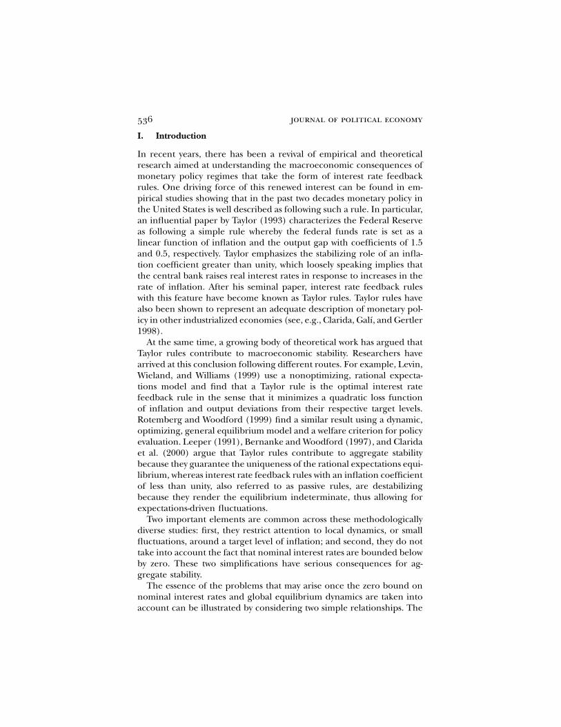
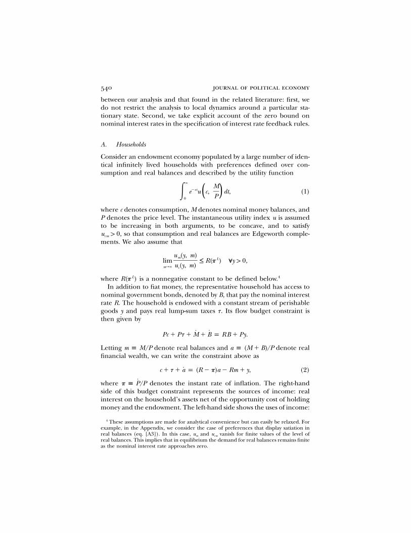
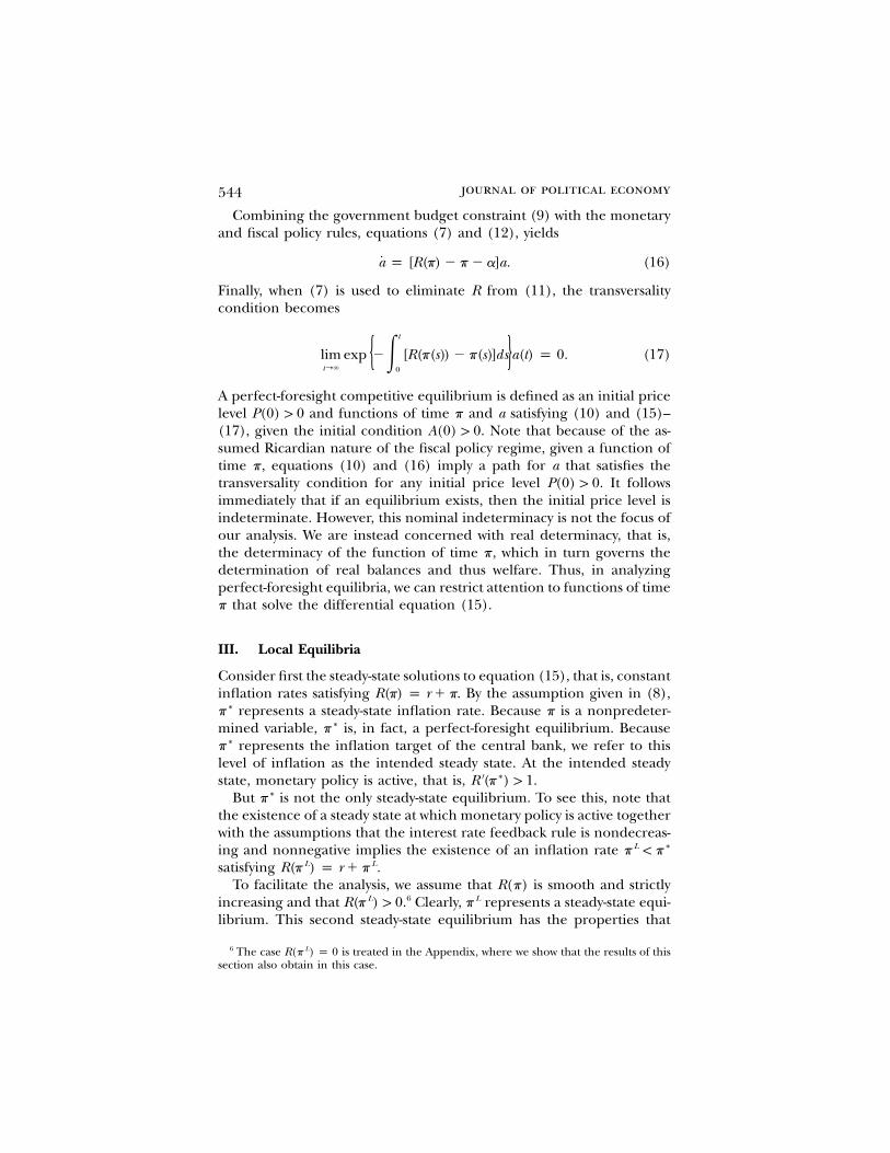
Fig. 1.—The liquidity trap in a flexible-price model

first one is an interest rate feedback rule whereby the nominalR p R(p)interest rate, R, is set as an increasing and nonnegative function of theinflation rate p. The second relationship is a steady-state Fisher equation,

stipulating that the nominal interest rate must equal the sumR p r � p,of the real interest rate r and inflation p (see fig. 1). Suppose that atthe target inflation rate the monetary authority follows a Taylor-type,∗p

or active, interest rate policy in the sense that Then, clearly′ ∗R (p ) 1 1.the presence of a zero bound on nominal interest rates and the as-sumption that the interest rate rule is increasing in inflation necessarilyimply the existence of a second inflation rate, at which the feedbackLp ,rule and the Fisher equation intersect. At this second intersection, in-flation is low and possibly negative, the nominal interest rate is low andpossibly zero, and monetary policy is passive, In Benhabib,′ LR (p ) ! 1.Schmitt-Grohe, and Uribe (2001b), we show, in the context of dynamic,optimizing, general equilibrium models, with and without nominal ri-gidities, that the unintended steady state is locally indeterminate.Lp

For in its neighborhood, equilibria exist in which inflation, interest rates,and aggregate activity fluctuate in response to nonfundamental revisionsin expectations. More important, the second steady state gives rise toequilibrium trajectories along which inflation and the nominal interestrate start arbitrarily close to the intended targets and con-∗ ∗(p , R(p ))verge gradually to 1L L(p , R(p )).

1 A branch of the literature has focused on the limitations that the zero bound onnominal interest rates imposes on the government’s ability to conduct countercyclicalmonetary policy. Model-based assessments of the costs associated with these limitations


When the economy falls into this type of decelerating inflation dy-namics, it is headed to a situation of low and possibly negative inflationand low and possibly zero interest rates in which monetary policy be-comes ineffective in bringing about the government’s goals regardingthe stability of output and prices. This state of affairs has all the essentialcharacteristics of a liquidity trap, at the heart of which there is a centralbank that is powerless to reverse the downward slide in prices throughexpansionary monetary policy in the form of lower and lower interestrates.2

The central focus of this paper is the design of fiscal and monetarypolicies that preserve the Taylor rule, and with it all its desirable localproperties, around the target rate of inflation and real activity, and atthe same time eliminate equilibrium dynamics leading to the liquiditytrap.

Two broad approaches to avoiding liquidity traps are presented. Inthe first one, liquidity traps are ruled out by means of fiscal policy whilemaintaining the assumption that monetary policy follows everywhere aninterest rate rule. The proposed stabilization policy features a strongfiscal stimulus that is automatically activated when inflation begins todecelerate. Specifically, the fiscal rule consists of an inflation-sensitivebudget surplus schedule that calls for lowering taxes when inflationsubsides. As the economy approaches the liquidity trap, fiscal deficitsbecome large enough that the low-inflation steady state becomes fiscallyunsustainable and ceases to be a rational expectations equilibrium. Thebasic insight that one can rule out liquidity traps by making them fiscallyunsustainable is due to Woodford (1999).

Our first approach to avoiding liquidity traps thus provides theoreticalsupport for the recent policy proposals—emanating most notably fromthe U.S. Department of the Treasury—suggesting that economies withnear-zero nominal interest rates and thus little room for monetary sta-bilization policy, such as Japan, should spend their way out of the li-quidity trap.3 However, we arrive at this policy recommendation for verydifferent reasons. The fiscal stimulus eliminates the liquidity trap notby using the traditional Keynesian multiplier, as is the conventional

are contained in Fuhrer and Madigan (1997), Orphanides and Wieland (1998), Reif-schneider and Williams (1999), and Wolman (1999).

2 In monetary economics, the term “liquidity trap” is used to describe a number ofdifferent but related phenomena. For instance, the standard textbook presentation ofliquidity traps is concerned with a situation in which the LM curve is horizontal, whichoccurs when the demand for real balances is perfectly elastic. Krugman (1998) refers toliquidity traps as episodes in which the nominal interest rate vanishes. Finally, in Woodford(1999), the term is used to describe equilibria in which real balances are at or above afinite satiation level for which the marginal utility of money is zero.

3 See, e.g., the June 24, 1998, testimony of Lawrence Summers, then–deputy secretaryof the Treasury, before a Senate Foreign Affairs subcommittee and his remarks to theWorld Economic Development Congress held on October 1, 1998, in Washington.


wisdom, but rather by affecting the intertemporal budget constraint ofthe government. The channel through which the liquidity trap is elim-inated here is more akin to Pigou’s argument on the implausibility ofliquidity traps. In a closed economy, the intertemporal budget constraintof the government is the mirror image of the intertemporal budgetconstraint of the representative household. A decline in taxes increasesthe household’s after-tax wealth, which induces an aggregate excessdemand for goods. As a consequence, the price level must increase inorder to reestablish equilibrium in the goods market.

The second approach consists of switching from an interest rate ruleto a money growth rate peg should inflation embark on a self-fulfillingdecelerating path. This alternative is a popular one, frequently men-tioned in the policy debate: when caught in a low-inflation equilibrium,governments should simply start printing money to jump-start the econ-omy. Krugman (1998), for example, argues forcefully for this type ofpolicy as a way to bring Japan out of its current recession. However, thisrecommendation is typically made without any reference to the accom-panying fiscal policy. As shown in Woodford (1999), a money growthrate rule is a successful tool to avoid or escape a liquidity trap only ifcoupled with the “right” fiscal policy. For instance, if the fiscal regimein place at the time of the switch to a money growth rule is one thatguarantees fiscal sustainability under all circumstances, then printingmoney may in fact be counterproductive since it is likely to acceleratethe deflationary spiral. In general, what is needed to make the switchto a money growth rate rule successful is a fiscal policy that, as nominalinterest rates approach zero, makes the government intertemporallyinsolvent.

The remainder of the paper is organized in five sections. Section IIpresents the model and the baseline monetary-fiscal regime. Section IIIcharacterizes local equilibrium dynamics. Section IV shows how theeconomy can fall into a liquidity trap when monetary policy takes theform of a Taylor-type interest rate feedback rule. Sections V and VIdevelop, respectively, fiscal and monetary instruments capable of elim-inating liquidity traps. Section VII closes the paper by discussing therobustness of the results to important model perturbations such as theintroduction of nominal frictions, the treatment of time as a discretevariable, and the adoption of Gesell taxes, which have been suggestedin the related literature as a possible way to avoid liquidity traps.

II. The Model

In this section we use a simple economic environment to illustrate howa monetary-fiscal regime frequently advocated on the basis of aggregatestability can in fact lead to expectational traps. There are two differences


between our analysis and that found in the related literature: first, wedo not restrict the analysis to local dynamics around a particular sta-tionary state. Second, we take explicit account of the zero bound onnominal interest rates in the specification of interest rate feedback rules.

A. Households

Consider an endowment economy populated by a large number of iden-tical infinitely lived households with preferences defined over con-sumption and real balances and described by the utility function

� M�rte u c, dt, (1)� ( )P0

where c denotes consumption, M denotes nominal money balances, andP denotes the price level. The instantaneous utility index u is assumedto be increasing in both arguments, to be concave, and to satisfy

so that consumption and real balances are Edgeworth comple-u 1 0,cm

ments. We also assume that

u (y, m)m Llim ≤ R(p ) Gy 1 0,u (y, m)mr� c

where is a nonnegative constant to be defined below.4LR(p )In addition to fiat money, the representative household has access to

nominal government bonds, denoted by B, that pay the nominal interestrate R. The household is endowed with a constant stream of perishablegoods y and pays real lump-sum taxes t. Its flow budget constraint isthen given by

˙ ˙Pc � Pt � M � B p RB � Py.

Letting denote real balances and denote realm { M/P a { (M � B)/Pfinancial wealth, we can write the constraint above as

˙c � t � a p (R � p)a � Rm � y, (2)

where denotes the instant rate of inflation. The right-hand˙p { P/Pside of this budget constraint represents the sources of income: realinterest on the household’s assets net of the opportunity cost of holdingmoney and the endowment. The left-hand side shows the uses of income:

4 These assumptions are made for analytical convenience but can easily be relaxed. Forexample, in the Appendix, we consider the case of preferences that display satiation inreal balances (eq. [A3]). In this case, um and ucm vanish for finite values of the level ofreal balances. This implies that in equilibrium the demand for real balances remains finiteas the nominal interest rate approaches zero.


consumption, tax payments, and savings. Households are also subjectto a borrowing limit of the form

t

lim exp � [R(s) � p(s)]ds a(t) ≥ 0, (3)�{ }tr� 0

which prevents them from engaging in Ponzi games. This no–Ponzigame constraint says that the household is not permitted to implementconsumption and money-holding plans that imply that its real debtposition net of money holdings grows at a rate higher than or equal tothe real interest rate. Clearly, because the utility function is increasingin consumption and real balances, the household will always find itoptimal to satisfy the borrowing limit above with equality. The repre-sentative household chooses paths for consumption, real balances, andwealth so as to maximize (1) subject to the flow budget constraint (2)and the borrowing limit (3), given its initial real wealth, a(0), and thepaths of taxes, inflation, and nominal interest rates. The associatedoptimality conditions are (2), (3) holding with equality, and

u (c, m) p l, (4)c

u (c, m) p lR, (5)m

and

l p l(r � p � R), (6)

where l is a Lagrange multiplier associated with the flow budgetconstraint.

B. Monetary and Fiscal Policy

We assume that the monetary authority follows an interest rate feedbackrule of the form

R p R(p). (7)

We refer to monetary policy as active at an inflation rate p if ′R (p) 1

and as passive if Loosely speaking, monetary policy is active′1 R (p) ! 1.if the central bank raises the real interest rate in response to an increasein inflation and is passive if the central bank fails to do so.

Three assumptions regarding the form of this feedback rule are ofgreat consequence for the subsequent results: first, we assume that thenominal interest rate is nondecreasing in inflation, that is, for′R (p) ≥ 0all p. Second, the interest rate feedback rule satisfies the zero boundon nominal interest rates in that, regardless of how low the inflation


rate may be, the monetary authority will never threaten to implementa negative nominal rate. Thus for all p. Third, we assume thatR(p) ≥ 0the central bank targets a rate of inflation and that, in the spirit∗p 1 �rof Taylor (1993), it conducts an active monetary policy around its in-flation target by responding to increases (decreases) in inflation with amore than one-for-one increase (decrease) in the nominal interest rate.Formally,

∗ ∗ ∗ ′ ∗ap 1 �r : R(p ) p r � p , R (p ) 1 1. (8)

The government finances its deficits by printing money, M, and issuingnominal bonds, B, that pay the nominal interest rate R. We assume thatpublic consumption is zero and that the government levies real lump-sum taxes, t. Therefore, the flow budget constraint of the governmentis given by which can be written as˙ ˙B p RB � M � Pt,

a p (R � p)a � Rm � t. (9)

By definition, the initial condition a(0) satisfies

A(0)a(0) p , (10)

P(0)

where denotes the initial level of total nominalA(0) { M(0) � B(0) 1 0government liabilities and is predetermined. Following Benhabib et al.(2001a), we classify fiscal policies as either Ricardian or non-Ricardian.5

Ricardian fiscal policies are those that ensure that the present dis-counted value of total government liabilities converges to zero, that is,

t

lim exp � [R(s) � p(s)]ds a(t) p 0 (11)�{ }tr� 0

is satisfied under all possible equilibrium or off-equilibrium paths ofendogenous variables, such as the price level, the money supply, infla-tion, or the nominal interest rate. In this subsection, we restrict attentionto one particular Ricardian fiscal policy that takes the form

t � Rm p aa, (12)

where the function of time a is chosen arbitrarily by the governmentsubject to the constraint that it is positive and bounded below by some

This policy states that consolidated government revenues, that is,a 1 0.tax revenues plus interest savings from the issuance of money, are alwayshigher than a certain fraction of total government liabilities. A speciala

case of this type of policy is a balanced-budget rule whereby tax revenues

5 Our definition of Ricardian fiscal policies is slightly different from that proposed inWoodford (1995).


are equal to interest payments on the debt. This case emerges whenprovided that R is bounded away from zero (Benhabib et al.a p R,

2001a).

C. Equilibrium

Equilibrium in the goods market requires that consumption be equalto the endowment

c p y. (13)

Given the assumptions regarding the form of the instant utility function,equations (4) and (5) implicitly define a liquidity preference functionof the form ; Because in equilibrium consump-m p l(c, R) l 1 0, l ! 0.c R

tion equals the endowment, which is assumed to be constant, in equi-librium real balances are only a function of the nominal interest rate.It then follows directly from (4) that the marginal utility of consumption,l, is a decreasing function of R:

′l p L(R); L ! 0. (14)

The reason why the marginal utility of consumption falls when thenominal interest rate increases is that real balances contract as the op-portunity cost of holding money rises. In turn, because consumptionand real balances are assumed to be Edgeworth complements ( ),u 1 0cm

in equilibrium the marginal utility of consumption increases with realbalances and thus falls with the nominal interest rate.

Use the feedback rule (7) to eliminate R from (6) and (14). Thentime-differentiate (14) and combine the resulting expression with (6)to obtain the following first-order differential equation in inflation:

�L(R(p))′ ˙R (p)p p [R(p) � p � r]. (15)′L(R(p))

The economics behind this differential equation are as follows: Supposethat the real interest rate exceeds the subjective rate of discount,

In this case, households will optimally choose a decliningR(p) � p 1 r.path for the marginal utility of consumption. But in the endowmenteconomy we are considering, the equilibrium marginal utility of con-sumption can fall only if real balances are expected to fall (recall thatreal balances and consumption are Edgeworth complements). Underthe implied liquidity preference function, a decline in real balancesrequires an increase in the opportunity cost of holding money, R. Giventhe interest rate feedback rule, an increase in the nominal interest ratewill be associated with an increase in the inflation rate, p 1 0.


Combining the government budget constraint (9) with the monetaryand fiscal policy rules, equations (7) and (12), yields

a p [R(p) � p � a]a. (16)

Finally, when (7) is used to eliminate R from (11), the transversalitycondition becomes

t

lim exp � [R(p(s)) � p(s)]ds a(t) p 0. (17)�{ }tr� 0

A perfect-foresight competitive equilibrium is defined as an initial pricelevel and functions of time p and a satisfying (10) and (15)–P(0) 1 0(17), given the initial condition Note that because of the as-A(0) 1 0.sumed Ricardian nature of the fiscal policy regime, given a function oftime p, equations (10) and (16) imply a path for a that satisfies thetransversality condition for any initial price level It followsP(0) 1 0.immediately that if an equilibrium exists, then the initial price level isindeterminate. However, this nominal indeterminacy is not the focus ofour analysis. We are instead concerned with real determinacy, that is,the determinacy of the function of time p, which in turn governs thedetermination of real balances and thus welfare. Thus, in analyzingperfect-foresight equilibria, we can restrict attention to functions of timep that solve the differential equation (15).

III. Local Equilibria

Consider first the steady-state solutions to equation (15), that is, constantinflation rates satisfying By the assumption given in (8),R(p) p r � p.

represents a steady-state inflation rate. Because p is a nonpredeter-∗p

mined variable, is, in fact, a perfect-foresight equilibrium. Because∗p

represents the inflation target of the central bank, we refer to this∗p

level of inflation as the intended steady state. At the intended steadystate, monetary policy is active, that is, ′ ∗R (p ) 1 1.

But is not the only steady-state equilibrium. To see this, note that∗p

the existence of a steady state at which monetary policy is active togetherwith the assumptions that the interest rate feedback rule is nondecreas-ing and nonnegative implies the existence of an inflation rate L ∗p ! p

satisfying L LR(p ) p r � p .To facilitate the analysis, we assume that R(p) is smooth and strictly

increasing and that 6 Clearly, represents a steady-state equi-L LR(p ) 1 0. p

librium. This second steady-state equilibrium has the properties that

6 The case is treated in the Appendix, where we show that the results of thisLR(p ) p 0section also obtain in this case.


monetary policy is passive and that the inflation rate is below the targetinflation rate.7 We refer to as the unintended or liquidity trap steadyLp

state.Consider now the existence of local equilibria other than the steady

states. Note that, because is always positive, the sign of in′ ′ ˙�L/LR p

equation (15) is the same as the sign of BecauseR(p) � p � r.it follows that near the active steady state is increasing′ ∗ ∗ ˙R (p ) 1 1, p , p

in p. Thus, if one limits the analysis to equilibria in which p remainsforever in a small neighborhood around then the only perfect-fore-∗p ,sight equilibrium is the active steady state itself, for all t. This∗p(t) p p

local uniqueness result has served as an important theoretical argumentfor advocating the use of active, or Taylor-type, interest rate feedbackrules to ensure aggregate stability (e.g., Leeper 1991; Woodford 1996;Clarida et al. 2000).8

If the economy is expected to remain forever near the inflation targetthen our model implies a relationship between the real interest rate∗p ,

and inflation that is quite standard. In particular, our model is consistentwith the mainstream intuition that when the Fed raises interest rates,inflation comes down. To understand the local equilibrium dynamicsimplied by the model, it is necessary to consider the question of howin our theoretical framework the real interest rate and inflation adjustto exogenous shocks. This type of exercise is necessary because, aspointed out above, in the absence of fundamental shocks, the onlyrational expectations equilibrium in which the rate of inflation remainsforever near the intended target is the target itself; that is, ∗p(t) p p

and for all t. Thus, in the absence of fundamental shocks,∗R(t) p R(p )no comovement between inflation and interest rates would ever be ob-served. In our model economy, the Taylor target is locally stable in thesense that exogenous fundamental shocks that push the system awayfrom the intended steady state give rise to dynamics that force the systemto return to the steady state. As we show in the next section, the dynamicsof the model can be very different when one allows for global equilibria,

7 In the context of the present flexible-price endowment economy, the low-inflationsteady-state equilibrium is, in fact, preferred to the target steady-state equilibriumLp

for it is associated with higher real balances and thus higher levels of utility. However,∗p ,as shown in Benhabib et al. (2001b), in the presence of nominal rigidities, the low-inflationequilibrium may be welfare inferior to the target steady state.

8 Note that if the assumption that real balances and consumption are Edgeworth com-plements ( ) is replaced with the assumption of Edgeworth substitutability ( ),u 1 0 u ! 0cm cm

then the perfect-foresight equilibrium is indeterminate in the sense that any initial inflationrate near the intended target gives rise to an inflation trajectory that converges to∗p

For a detailed analysis of this case, see Benhabib et al. (2001a). That paper shows that∗p .the local equilibrium dynamics in the case in which ucm is negative are qualitatively identicalto those arising in a model in which money enters in the production function, so thatfirms’ costs are increasing in the level of the nominal interest rate.


that is, equilibria in which the economy may move permanently awayfrom the Taylor target.

The local equilibrium dynamics in the neighborhood of the low-inflation steady state are quite different from those around the targetLp

steady state Since it follows that is decreasing in p for∗ ′ L ˙p . R (p ) ! 1, p

p near This implies that inflation trajectories originating in theLp .vicinity of converge to and thus can be supported as perfect-L Lp p

foresight equilibria. Therefore, the low-inflation steady state is not lo-cally unique.9 This is one of the reasons why passive monetary policy isconsidered destabilizing.

IV. Falling into Liquidity Traps

A focal point of this paper is to draw attention to the fact that in additionto the local equilibria described in Section III, there exists a large num-ber of equilibrium trajectories originating arbitrarily close to (and tothe left of) the intended target that converge smoothly and mono-∗p

tonically to the unintended, or liquidity trap, steady state (see fig.Lp

1).10 Along such equilibrium paths, the central bank, following the pre-scription of the Taylor rule, continuously eases in an attempt to reversethe persistent decline in inflation. But these efforts are in vain, andindeed counterproductive, for they introduce further downward pres-sure on inflation. This state of matters, in which monetary policy failsto stop the deceleration in prices, is central to the notion of a liquiditytrap. Another aspect of these dynamics that is central to the concept ofliquidity traps is their self-fulfilling nature: all that is needed to fall intothe liquidity trap is that people expect the economy to slide into a phaseof decelerating inflation.

The intuition behind the result that a Taylor target may open thedoor to liquidity traps is as follows. Suppose that the public expectsinflation to fall in the future. Then, because monetary policy is publicknowledge, agents also expect the nominal interest rate to fall. In turn,the expected decline in nominal interest rates will be associated withan expected increase in the demand for real balances and hence withan expected increase in the marginal utility of consumption (recall ourmaintained assumption that and that in equilibrium agents al-u 1 0cm

ways expect consumption to be constant). But optimizing householdswill expect the marginal utility of consumption to increase only if the

9 The local indeterminacy of equilibrium around gives rise to aggregate instabilityLpin the form of stationary sunspot equilibria. For a general result on the existence ofstationary sunspot equilibria in continuous-time models displaying local indeterminacy ofthe perfect-foresight equilibrium, see Shigoka (1994).

10 As is clear from the figure, there also exist hyperinflationary trajectories originatingto the right of These equilibrium paths, however, are not the focus of our study.∗p .


current real interest rate is below the rate of time preference. Becausethe Fed follows a Taylor rule, the real interest rate is below the rate oftime preference only when current inflation is below the Taylor target.The circle closes because expectations of future declines in inflationcan be supported as equilibrium outcomes when the current inflationrate is below the Taylor target. It is in this particular sense that in thiseconomy expectations of future declines in inflation and the nominalinterest rate can be self-fulfilling.

When these expectational dynamics take hold of the economy, theusual intuition about the relation between real interest rates and infla-tion breaks down. A decline in the rate of inflation may now be initiatedpurely by expectations of future declines in inflation, and the Fed’sactive response of lowering the nominal and real interest rates cannotcontain the ensuing path descending into a liquidity trap. This is pre-cisely why it is so difficult to understand the dynamics of liquidity trapsin general and Japan’s current slump in particular: in spite of the centralbank’s aggressive lowering of interest rates, inflation, far from pickingup, keeps edging down.

V. Avoiding Liquidity Traps through Fiscal Policy

In this section, we develop policy schemes designed to eliminate theliquidity trap. The strategy is to modify fiscal policy while maintainingthe assumed monetary policy. Specifically, we consider fiscal adjustmentmechanisms that are automatically activated whenever the economy em-barks on a self-fulfilling path of decelerating inflation. These mecha-nisms will rule out liquidity traps by making the low-inflation steady statefiscally unsustainable.

A. An Inflation-Sensitive Revenue Schedule

Consider replacing the Ricardian fiscal policy given by (12) with onein which the coefficient a, reflecting the sensitivity of consolidated gov-ernment revenues with respect to the level of total government liabilities,is an increasing function of the inflation rate. Specifically, the fiscalpolicy now takes the form

′t � Rm p a(p)a; a 1 0. (18)

We impose the following additional restrictions on the function a:∗a(p ) 1 0 (19)

andLa(p ) ! 0. (20)


This policy guarantees that the intended steady state is a perfect-∗p

foresight equilibrium and at the same time rules out the liquidity trapas an equilibrium outcome. To see this, combine (18) and the TaylorLp

rule (7) with the instant government budget constraint (9) to obtainthe following equilibrium law of motion for a:

a p [R(p) � p � a(p)]a. (21)

Solving this differential equation, one obtains

t

a(t) p exp [R(p(s)) � p(s) � a(p(s))]ds a(0),�{ }0

which implies that

t t

lim exp � [R(s) � p(s)]ds a(t) p a(0) lim exp � a(p(s))ds . (22)� �{ } [ ]tr� tr�0 0

Consider a constant inflation trajectory By condition (19), the∗p p p .right-hand side of (22) equals zero. Therefore, the transversality con-dition is satisfied and represents a perfect-foresight equilibrium.∗p p p

On the other hand, for an inflation trajectory in which p convergesto the liquidity trap condition (20) implies that the right-hand sideLp ,of (22) does not converge to zero (except in the special case in whichinitial total government liabilities, a(0), are exactly equal to zero), thusviolating the transversality condition. As a result, no inflation path lead-ing to the liquidity trap can be supported as an equilibrium outcome.

Under the proposed inflation-sensitive revenue schedule, the govern-ment manages to fend off the unintended low-inflation equilibrium bythreatening to implement a fiscal stimulus package consisting of a severeincrease in the consolidated deficit should the inflation rate becomesufficiently low. Interestingly, this type of policy prescription is what theU.S. Treasury and a large number of academic and professional econ-omists are advocating as a way for Japan to lift itself out of its currentdeflationary trap. However, we arrive at this policy recommendation forvery different reasons. The fiscal stimulus we propose eliminates theliquidity trap not by using the traditional Keynesian multiplier, as is theconventional wisdom, but rather by affecting the intertemporal budgetconstraint of the government. The channel through which the liquiditytrap is eliminated here is more akin to Pigou’s argument on the im-plausibility of liquidity traps. In a closed economy, the intertemporalbudget constraint of the government is the mirror image of the inter-temporal budget constraint of the representative household. A declinein taxes increases the household’s after-tax wealth, which induces anaggregate excess demand for goods. With aggregate supply fixed, the


price level must increase in order to reestablish equilibrium in the goodsmarket.

1. Targeting the Growth Rate of Nominal Government Liabilities

The following example to rule out liquidity traps under interest ratefeedback rules was first suggested by Woodford (1999). In this example,the fiscal policy rule consists in pegging the growth rate of total nominalgovernment liabilities. That is,

Ap k, (23)

A

where k is assumed to satisfyL ∗R(p ) ! k ! R(p ). (24)

Clearly, this condition implies that at the liquidity trap ( ), total nom-Lp

inal government liabilities grow at a rate larger than the nominal interestrate. Thus, as the economy approaches the liquidity trap, the presentdiscounted value of government liabilities does not converge to zero.Therefore, such paths for the inflation rate cannot be supported asequilibrium outcomes. Formally, expressing as and com-˙ ˙A/A (a/a) � p

bining the fiscal policy rule above with the instant government budgetconstraint (9) yields

t � Rm p [R(p) � k]a.

Thus this fiscal policy rule is a special case of the one given in equation(18) when a(p) takes the form In particular, note that, becauseR(p) � k.the Taylor rule is increasing in the rate of inflation, so is R(p) � k.Furthermore, condition (24) implies that restrictions (19) and (20) aresatisfied. It follows immediately that targeting the growth rate of nominalgovernment liabilities is a potential way of eliminating equilibrium de-flationary spirals.

2. A Balanced-Budget Requirement

Consider now a fiscal policy rule consisting of a zero secondary deficit,that is, where B denotes outstanding interest-bearing publicPt p RB,debt. This policy rule requires that the government equates its primarysurplus, Pt, to interest payments on the public debt, RB, so that thesecondary deficit, given by is always equal to zero. RecallingRB � Pt,that we can rewrite the balanced-budget rule asa p (B/P) � m,

t � Rm p R(p)a. (25)


It follows that a balanced-budget requirement is also a special case ofthe fiscal policy rule given in (18) in which Clearly, in thisa(p) p R(p).case a(p) is increasing because so is R(p). Condition (19) is satisfiedbecause by assumption. On the other hand, condition (20)∗R(p ) 1 0is not satisfied because of our maintained assumption that LR(p ) 1 0.However, if one relaxes this assumption by considering the case of aTaylor rule that stipulates zero nominal interest rates at sufficiently lowrates of inflation, it becomes clear that a balanced-budget rule eliminatesthe liquidity trap as long as nominal interest rate paths leading to theliquidity trap satisfy 11 To see why, note that under atlim R(s)ds ! �.∫0tr�

balanced-budget rule, by (9) and (25), the law of motion of real totalgovernment liabilities is given by Using this expression, wea p �pa.can write the transversality condition (11) as

t

lim a(0) exp � R(s)ds p 0.�[ ]tr� 0

In the Appendix, we present two examples involving a Taylor rule thatsets the nominal interest rate to zero at low rates of inflation. In oneof the examples, paths leading to the liquidity trap feature nominalinterest rates that converge to zero but never actually reach that floor.In the other example, the nominal interest rate reaches the zero boundin finite time. We show that in both cases a balanced-budget rule suc-ceeds in averting the liquidity trap. These examples show that it is inprinciple possible to escape the liquidity trap without the threat of gen-erating fiscal deficits. What is crucial, however, is a commitment of thecentral bank to lower nominal interest rates all the way to zero as in-flation becomes sufficiently low. Any interest rate feedback rule lackingthis strong commitment leaves the door open to unintended deflation-ary spirals.

VI. Avoiding Liquidity Traps through a Monetary Regime Switch

Thus far, we have studied the design of fiscal policies capable of elim-inating liquidity traps when the monetary authority follows an interestrate feedback rule that is valid globally (i.e., for all possible values ofthe inflation rate). An alternative route to avoiding self-fulfilling liquiditytraps is to modify monetary policy when the economy seems to beheaded toward a low-inflation spiral. For example, in the case of Japan,a frequently advocated strategy to lift the economy out of deflation isfor the Bank of Japan to switch to a money growth rate target letting

11 This is how Schmitt-Grohe and Uribe (2000) rule out liquidity traps in a discrete-time cash-in-advance economy with cash and credit goods.


interest rates be market determined. In this section, we show that aban-doning an interest rate feedback rule in favor of a monetary target wheninflation reaches dangerously low levels can be a successful way to avoidfalling into a deflationary trap, but it need not be. The effectiveness ofsuch an alternative will in general depend on the accompanying fiscalregime. We illustrate this general conclusion by means of two examples.

A. Switching to a Money Growth Rule Is Ineffective When Fiscal Policy IsRicardian

We begin by showing that under the Ricardian fiscal policy rule givenby (12), switching from an interest rate feedback rule to a money growthrate rule as the nominal interest rate gets close to zero will not eliminateself-fulfilling deflations. To establish this result, it is enough to showthat under this fiscal regime, self-fulfilling deflations exist even undera money growth rate rule.12 Specifically, assume that monetary policytakes the form

Mp m, (26)

M

where is a constant.13 This monetary policy implies thatm 1 �r

mp m � p. (27)

m

A perfect-foresight equilibrium can then be defined as functions of timec, m, p, l, and R satisfying (4), (5), (6), (13), and (27). As we haveshown above, under the assumed fiscal policy the transversality condition(17) is always satisfied, so we do not include it in our definition ofequilibrium. Combining the equilibrium conditions yields the followingdifferential equation in real balances:

r � m � [u (y, m)/u (y, m)]m cm p . (28)

(1/m) � [u (y, m)/u (y, m)]cm c

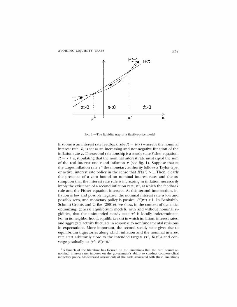
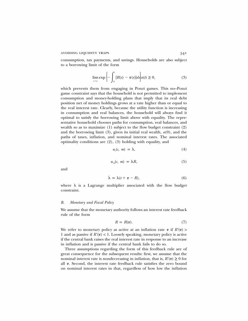
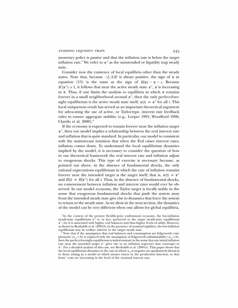
Any function of time m satisfying this differential equation representsa perfect-foresight equilibrium. Figure 2 depicts the correspondingphase diagram. Because m is a jump variable, one possible equilibrium

12 This finding is due to Woodford (1999). We repeat the argument here to make thepresentation self-contained.

13 Note that we allow for both positive and negative rates of monetary expansion. Thisis of interest for the results that follow because under the fiscal regime typically assumedin the literature on speculative deflations (namely, at all times), self-fulfilling de-B p 0flations occur only for negative money growth rates (Woodford 1994).


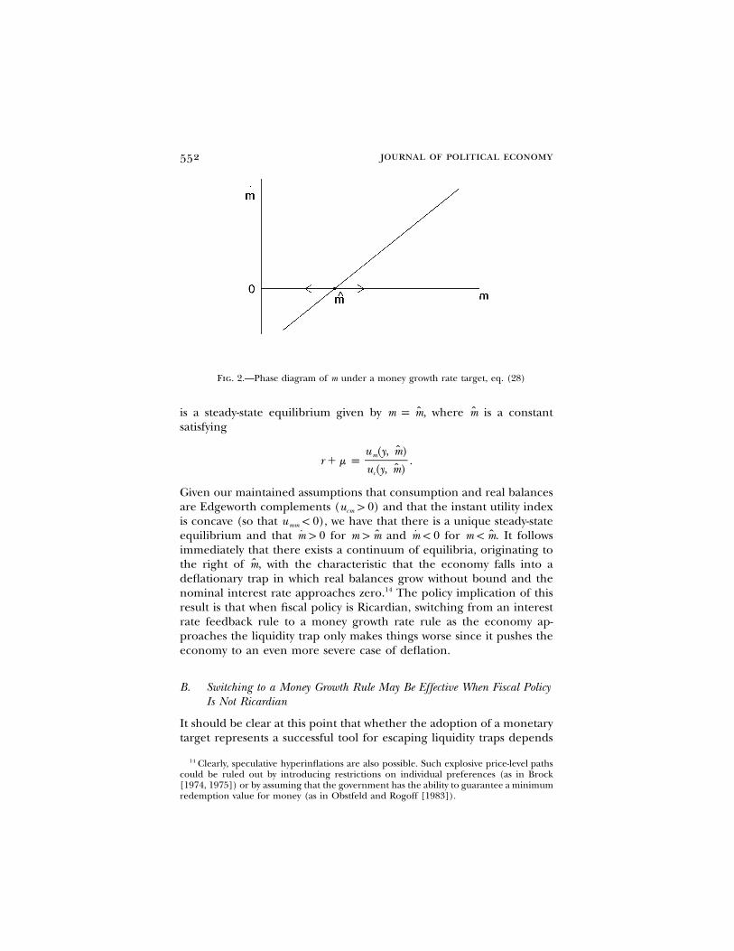
Fig. 2.—Phase diagram of m under a money growth rate target, eq. (28)

is a steady-state equilibrium given by where is a constantˆ ˆm p m, msatisfying

û (y, m)mr � m p .

û (y, m)c

Given our maintained assumptions that consumption and real balancesare Edgeworth complements ( ) and that the instant utility indexu 1 0cm

is concave (so that ), we have that there is a unique steady-stateu ! 0mm

equilibrium and that for and for It follows˙ ˆ ˙ ˆm 1 0 m 1 m m ! 0 m ! m.immediately that there exists a continuum of equilibria, originating tothe right of with the characteristic that the economy falls into am,deflationary trap in which real balances grow without bound and thenominal interest rate approaches zero.14 The policy implication of thisresult is that when fiscal policy is Ricardian, switching from an interestrate feedback rule to a money growth rate rule as the economy ap-proaches the liquidity trap only makes things worse since it pushes theeconomy to an even more severe case of deflation.

B. Switching to a Money Growth Rule May Be Effective When Fiscal PolicyIs Not Ricardian

It should be clear at this point that whether the adoption of a monetarytarget represents a successful tool for escaping liquidity traps depends

14 Clearly, speculative hyperinflations are also possible. Such explosive price-level pathscould be ruled out by introducing restrictions on individual preferences (as in Brock[1974, 1975]) or by assuming that the government has the ability to guarantee a minimumredemption value for money (as in Obstfeld and Rogoff [1983]).


crucially on the assumed fiscal stance. As the previous discussion dem-onstrates, when fiscal policy is Ricardian, a switch to a monetary targetis likely to be counterproductive. However, the central result of thissubsection is that when fiscal policy is not Ricardian, the monetaryauthority may be able to inflate its way out of a liquidity trap by targetinga sufficiently high rate of money growth.

We convey this argument by studying a fiscal regime under whichtrajectories leading to a liquidity trap are possible when monetary policytakes the form of an interest rate feedback rule like (7) but are im-possible when the central bank controls the rate of expansion of themonetary aggregate. We then use this insight to construct a monetaryregime that keeps the appealing properties of a Taylor rule in the neigh-borhood of the target rate of inflation and eliminates the possibility∗p

of liquidity traps by switching to a money growth rate rule when theeconomy approaches the low-inflation steady state Lp .

Consider, for example, a fiscal policy whereby public debt is exoge-nous, nonnegative, and bounded by an exponential function of time.Specifically,

gt¯ ¯0 ≤ B(t) ≤ Be ; B ≥ 0. (29)

This expression defines a family of fiscal policies that includes a numberof special cases frequently considered in monetary economics. Perhapsthe most commonly assumed fiscal regime is one in which public debtequals zero at all times ( ). It also includes policies that limitB(t) p 0the growth rate of public debt such as the Maastricht criterion, whichsets an upper bound on debt of 60 percent of gross domestic product( and ).B p 0.6y g p 0

To see that fiscal policies belonging to the class defined in (29) arenot Ricardian, consider, for example, a trajectory of nominal interestrates converging to a constant less than g. Clearly, in this case the presentdiscounted value of public debt converges to infinity, violating the trans-versality condition (11).

We begin by showing that if the fiscal policy restriction (29) is com-bined with the interest rate feedback rule (7), then self-fulfilling liquiditytraps may occur in equilibrium. For the analysis that follows, it will proveconvenient to rewrite the equilibrium conditions in terms of sequencesfor real balances and nominal debt rather than in terms of inflationand real wealth, as we did in Section IIC. Combining (4)–(7) and (13)yields

u (y, m)cm p [r � p(m) � R(p(m))], (30)

u (y, m)cm


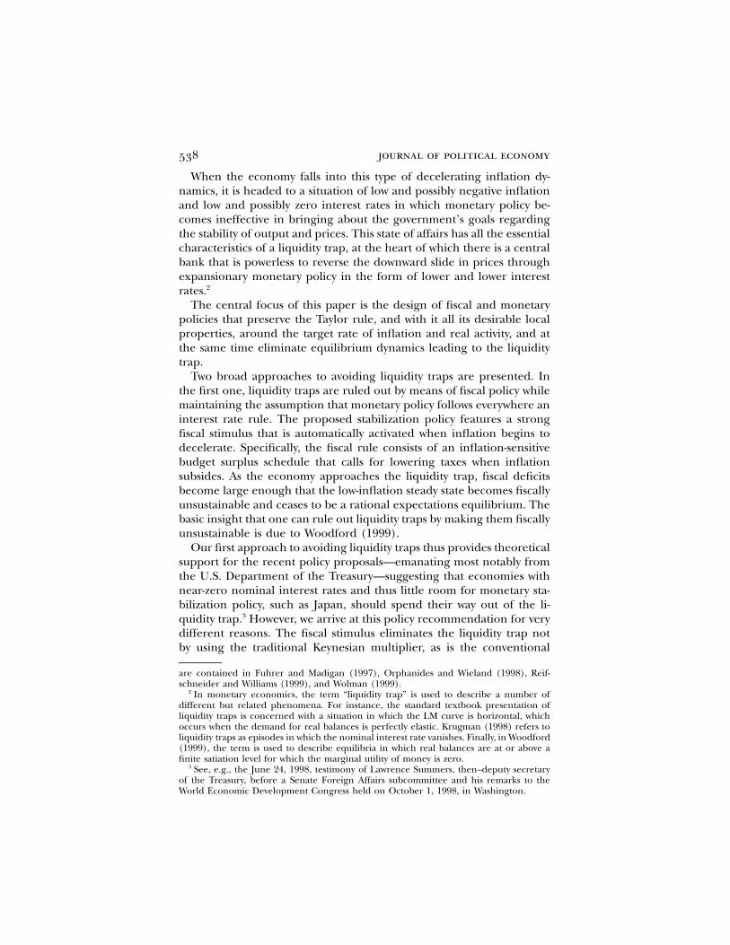
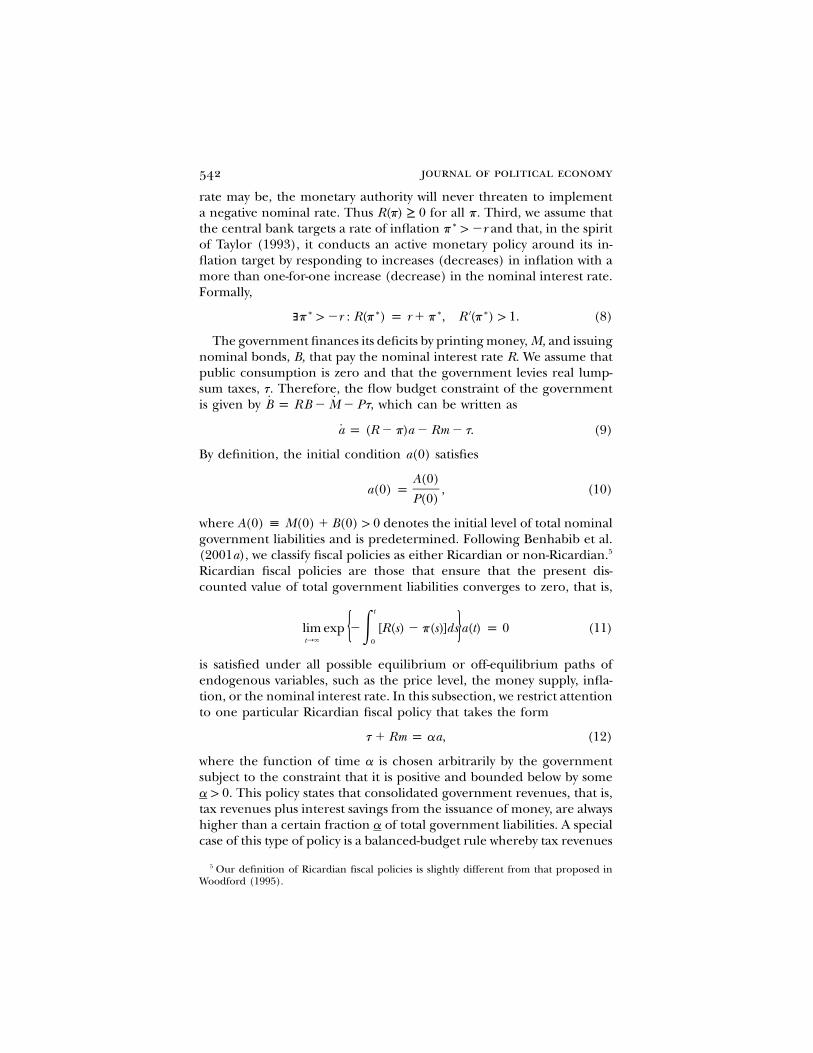
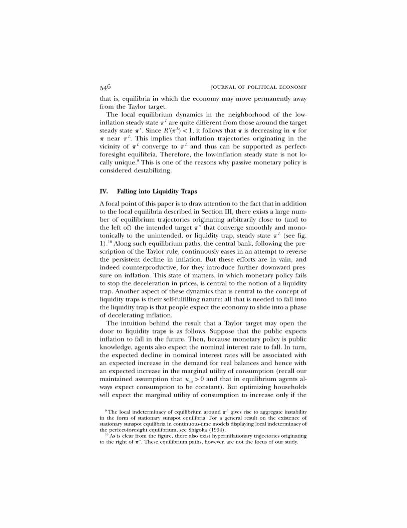
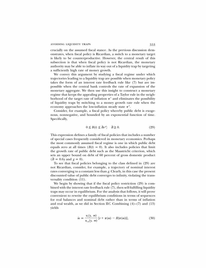
Fig. 3.—Phase diagram of m under an interest rate feedback rule, eq. (30)

where p(m) is a strictly decreasing function implicitly defined by

u (y, m)mp R(p).

u (y, m)c

The transversality condition (17) and the initial condition (10) become,respectively,

t

lim exp � [R(p(m(s))) � p(m(s))]ds m(t)�{ }tr� 0

tB(t)

� exp � R(p(m(s)))ds p 0 (31)�[ ]P(0)0

and

P(0)m(0) � B(0) p A(0). (32)

A perfect-foresight equilibrium is defined as a function of time m andan initial price level satisfying (30)–(32), given an exogenousP(0) 1 0function of time B satisfying (29) and A(0) 1 0.

Figure 3 displays the phase diagram associated with equation (30),which, of course, is qualitatively equivalent to that corresponding toequation (15) and shown in figure 1. In particular, there exists a steadystate associated with the target inflation rate and a steady state∗ ∗m , p ,

associated with the low inflation rate that is, with the li-L ∗ Lm 1 m , p ,quidity trap.

But there exist other solutions to the differential equation (30). Spe-cifically, there exists an infinite number of trajectories of real balancesthat originate in the vicinity of and converge to as well as aL Lm mcontinuum of trajectories starting in a neighborhood to the right of


that also converge to These trajectories will represent perfect-∗ Lm m .foresight equilibria if they satisfy the transversality condition (31). Tothe extent that or equation (31) will hold for anyL ¯g ! R(p(m )) B p 0,trajectory m converging to Therefore, if or thereL L ¯m . g ! R(p(m )) B p 0,is a continuum of perfect-foresight equilibria starting arbitrarily closeto the intended steady state that lead to the liquidity trap 15∗ Lm m .

On the other hand, when monetary policy takes the form of a moneygrowth rate rule like the one given by equation (26) with them ≥ 0,large number of perfect-foresight equilibria that arise under the interestrate feedback rule (7) are reduced to a unique one. To see this, notethat in this case a perfect-foresight equilibrium is a function of time msatisfying (28) and the transversality condition (17), which can be writ-ten as

t u (y, m)mlim exp � � m ds M(0)�{ [ ] }u (y, m)tr� 0 c

t u (y, m)m� exp � ds B(t) p 0, (33)�[ ]u (y, m)0 c

given an exogenous function of time B satisfying (29) and the initialcondition M(0) 1 0.

We have already characterized the solutions to the differential equa-tion (28), which are summarized in figure 2: there exists a unique steadystate and a continuum of trajectories starting to the right of andˆ ˆm mconverging to infinity. However, under the fiscal policy considered here,none of the solutions in which real balances grow without bound canbe supported as a competitive equilibrium. The reason is that as mconverges to infinity, the nominal interest rate, con-u (y, m)/u (y, m),m c

verges to zero, implying, given the maintained assumption of a non-negative rate of money growth, that the first term of the transversalitycondition (33) fails to approach zero as t gets large. As a result, underthe fiscal policy restriction (29), a money growth rate peg is a successfultool to fend off self-fulfilling liquidity traps.

1. A Monetary Policy Regime Switch

An interesting question that emerges from the results above is whetherthe central bank could design a monetary policy that takes the form ofa Taylor rule near the inflation target and switches to a money growth∗p

rate rule when the economy appears to be sliding into a liquidity trap.

15 To complete the characterization of equilibrium, we note that, in contrast to the caseunder the Ricardian fiscal policy (12), the equilibrium displays nominal determinacy inthe sense that, given functions B and m, P(0) is uniquely determined by (32).


One obstacle that the construction of such a policy switch must tackleis to prevent an anticipated discrete jump in the price level at the timeof the regime change. Besides price-level smoothing, central bank be-havior in developed countries has been described as pursuing a smoothrate of inflation. This characterization is reflective of the observed re-markable inflation inertia. In the context of our model, the equilibriumprice level and inflation rate are continuous if real balances and theirtime derivative are continuous.16 Accordingly, we show how to design amonetary policy switch from a Taylor rule to a money growth rate rulethat eliminates the liquidity trap while guaranteeing continuity of m andm.

Let be the threshold value of real balances below which the centralmbank follows the interest rate feedback rule given by (7) and abovewhich it pegs the growth rate of the money supply as described byequation (26). The dynamics of real balances are therefore given by(30) for and by (28) for That is,˜ ˜m ≤ m m 1 m.

u (y, m)c ˜[r � p(m) � R(p(m))] for m ≤ mu (y, m)cm

�1m p (34)1 u (y, m) u (y, m)cm m{ ˜� r � m � for m 1 m.[ ] [ ]m u (y, m) u (y, m)c c

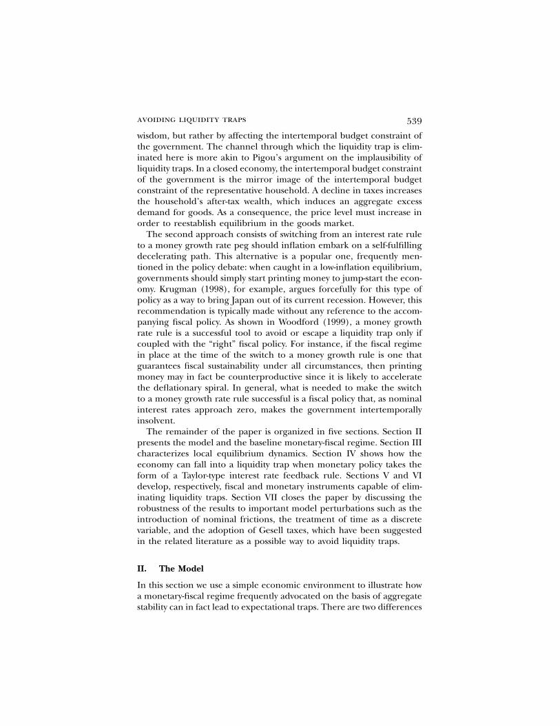
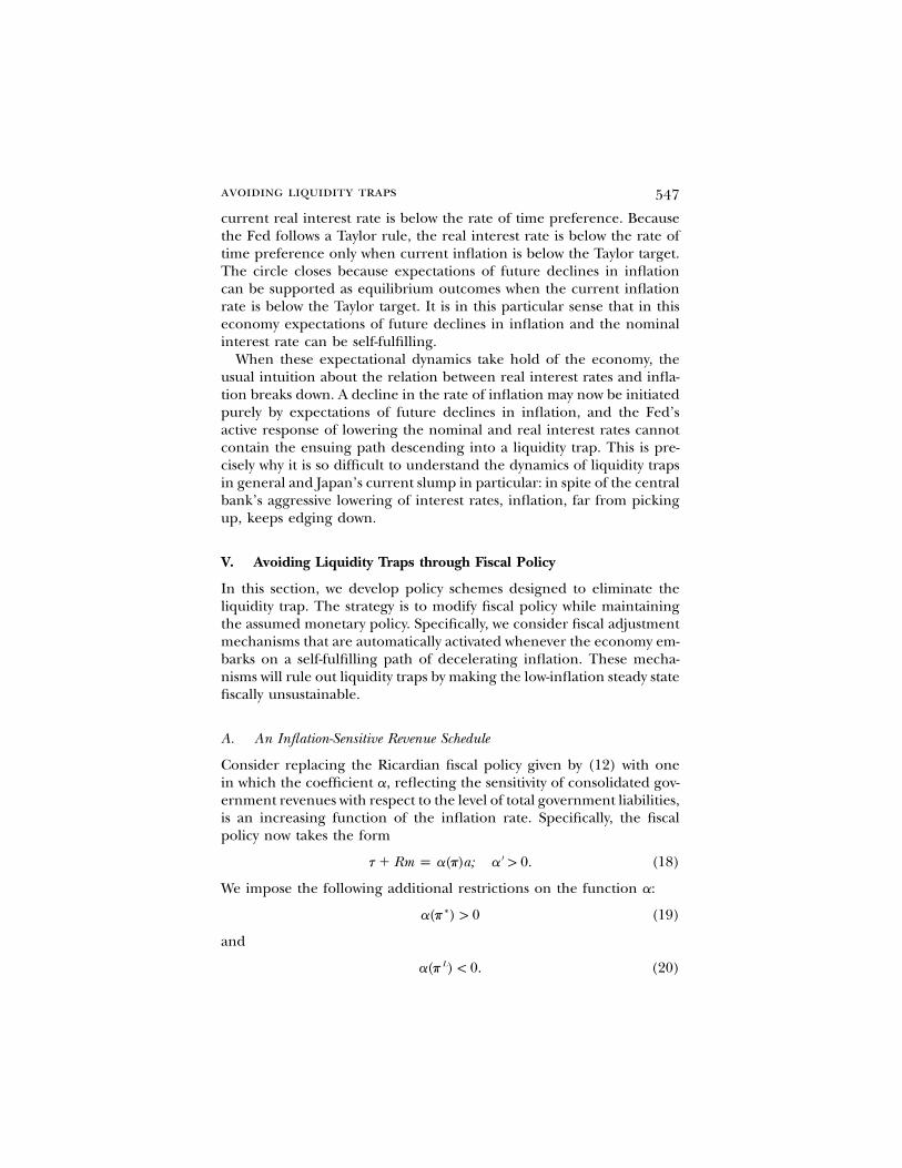
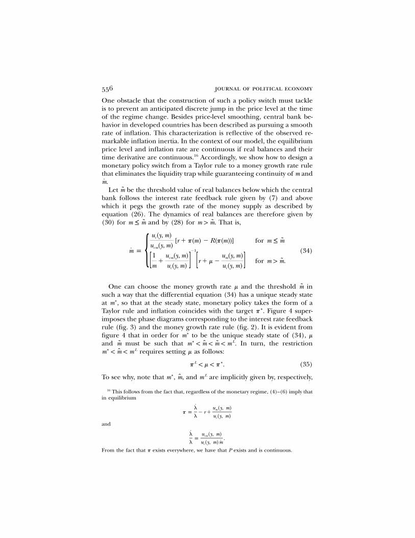
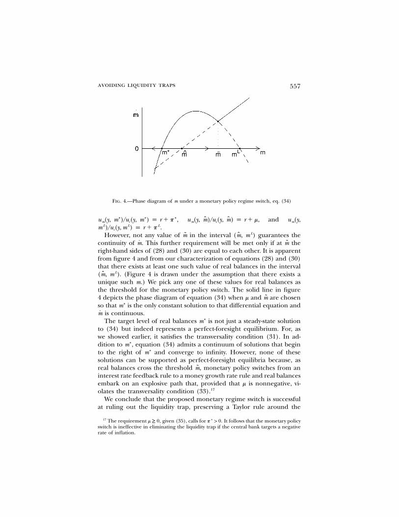
One can choose the money growth rate m and the threshold inmsuch a way that the differential equation (34) has a unique steady stateat so that at the steady state, monetary policy takes the form of a∗m ,Taylor rule and inflation coincides with the target Figure 4 super-∗p .imposes the phase diagrams corresponding to the interest rate feedbackrule (fig. 3) and the money growth rate rule (fig. 2). It is evident fromfigure 4 that in order for to be the unique steady state of (34), m∗mand must be such that In turn, the restriction∗ L˜ ˆ ˜m m ! m ! m ! m .

requires setting m as follows:∗ Lˆm ! m ! m

L ∗p ! m ! p . (35)

To see why, note that and are implicitly given by, respectively,∗ Lˆm , m, m

16 This follows from the fact that, regardless of the monetary regime, (4)–(6) imply thatin equilibrium

l u (y, m)mp p � r �

l u (y, m)c

and

l u (y, m)cmp .

˙l u (y, m)mc

From the fact that p exists everywhere, we have that P exists and is continuous.


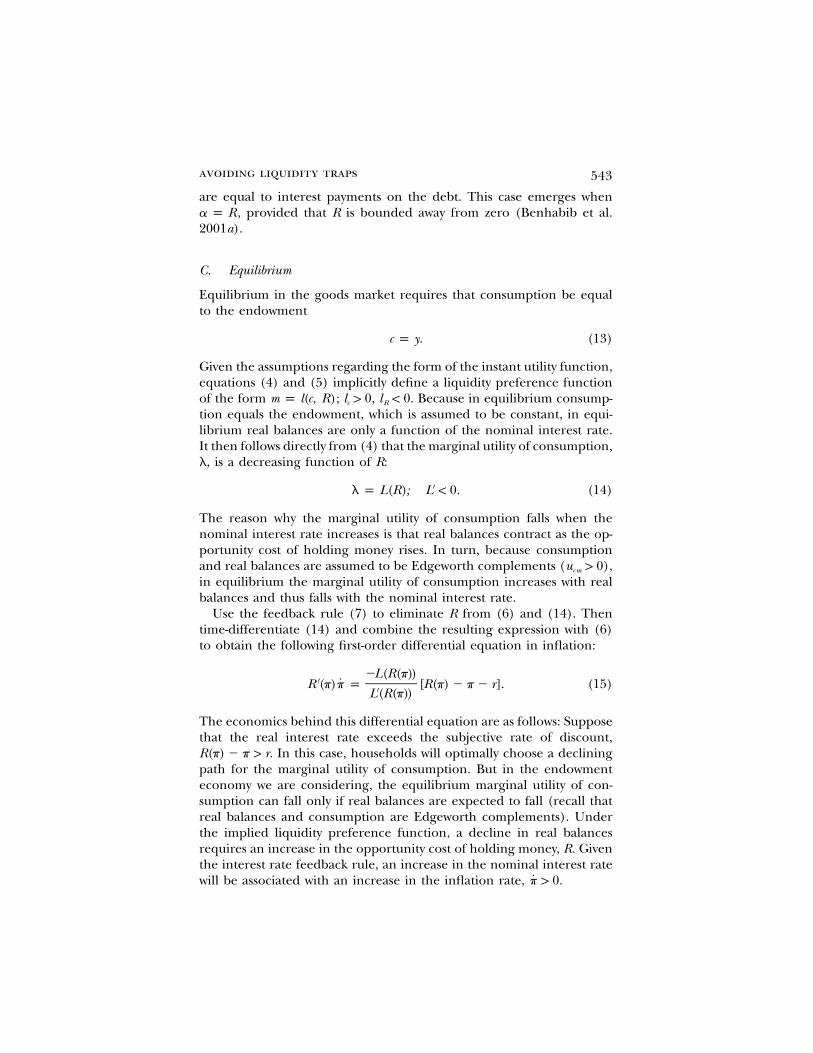
Fig. 4.—Phase diagram of m under a monetary policy regime switch, eq. (34)

and∗ ∗ ∗ ˆ û (y, m )/u (y, m ) p r � p , u (y, m)/u (y, m) p r � m, u (y,m c m c mL L Lm )/u (y, m ) p r � p .c

However, not any value of in the interval guarantees theL˜ ˆm (m, m )continuity of This further requirement will be met only if at the˙ ˜m. mright-hand sides of (28) and (30) are equal to each other. It is apparentfrom figure 4 and from our characterization of equations (28) and (30)that there exists at least one such value of real balances in the interval

(Figure 4 is drawn under the assumption that there exists aLˆ(m, m ).unique such m.) We pick any one of these values for real balances asthe threshold for the monetary policy switch. The solid line in figure4 depicts the phase diagram of equation (34) when m and are chosenmso that is the only constant solution to that differential equation and∗m

is continuous.mThe target level of real balances is not just a steady-state solution∗m

to (34) but indeed represents a perfect-foresight equilibrium. For, aswe showed earlier, it satisfies the transversality condition (31). In ad-dition to equation (34) admits a continuum of solutions that begin∗m ,to the right of and converge to infinity. However, none of these∗msolutions can be supported as perfect-foresight equilibria because, asreal balances cross the threshold monetary policy switches from anm,interest rate feedback rule to a money growth rate rule and real balancesembark on an explosive path that, provided that m is nonnegative, vi-olates the transversality condition (33).17

We conclude that the proposed monetary regime switch is successfulat ruling out the liquidity trap, preserving a Taylor rule around the

17 The requirement given (35), calls for It follows that the monetary policy∗m ≥ 0, p 1 0.switch is ineffective in eliminating the liquidity trap if the central bank targets a negativerate of inflation.


target rate of inflation and guaranteeing the continuity of the price∗p ,level and inflation.

VII. Discussion and Conclusion

The zero bound on nominal interest rates makes economies in whichmonetary policy takes the form of an interest rate feedback rule proneto unintended equilibrium outcomes. When these undesirable circum-stances occur, the monetary authority finds itself powerless to bringabout the policy objectives of the government. It is precisely this inabilityof monetary policy to affect key macroeconomic variables, such as thelevel of inflation and the volatility of output and prices, that is at theheart of the concept of a liquidity trap.

Besides the explicit consideration of the zero bound on nominalinterest rates, perhaps the most notable difference between our modeland those that stress the desirability of Taylor rules is the absence ofnominal rigidities. However, the possibility of falling into a liquidity trapas a consequence of Taylor-type rules is not limited to the simple flexible-price environment presented in this paper. In Benhabib et al. (2001b),we show that Taylor rules also engender liquidity traps in environmentswith sluggish price adjustment. In this type of model, the liquidity trapinvolves indeterminacy not only of inflation and real balances, as in themodel considered in this paper, but also of the level of aggregate de-mand. The policy recommendations aimed at eradicating liquidity trapsproposed in Sections V and VI are also effective in economies with stickyprices. For those recommendations involve the violation of a transver-sality condition in the event that the economy falls into a liquidity trap.The violation of this long-run restriction depends on the asymptoticbehavior of the endogenous variables of the model, which is indepen-dent of short-run nominal price rigidities.

A further difference between the theoretical environment consideredin this paper and that studied in part of the related literature is ourtreatment of time as a continuous variable. Again, neither the existenceof a liquidity trap emerging as a consequence of the adoption of a Taylorrule nor the effectiveness of the proposed remedies is affected by thisassumption in any important way. Schmitt-Grohe and Uribe (2000) an-alyze a discrete-time cash-in-advance model with cash and credit goodsand show that a Taylor rule in combination with a lower bound onnominal rates gives rise to an unintended liquidity trap. Because thenature of this undesirable equilibrium is identical to that identified inthis paper, the long-run restrictions that are capable of eliminating li-quidity traps in the continuous-time model will also be applicable underdiscrete time.

The policies considered in this paper can be viewed as intended to


eliminate undesirable dynamics that may arise under Taylor rules. Forthe proposed policies to be effective, it is important that under theundesired dynamics, inflation moves forever away from its intendedtarget. In Benhabib et al. (2000), we show that Taylor rules can giverise to unintended dynamics that are of a different nature than the onesconsidered in this paper. Specifically, we find that when monetary policyfollows the Taylor principle, chaotic dynamics may arise. Under thesedynamics the economy fluctuates in a potentially large neighborhoodaround the equilibrium intended by the central bank but never fallsinto a self-fulfilling deflation, or liquidity trap, of the type analyzed here.Thus the specific policies described in this paper may not be successfulin eliminating these chaotic equilibria since they rely on the conver-gence of inflation to a permanently lower level.18

Buiter and Panigirtzoglou (1999) have proposed the use of Geselltaxes (or taxes on money holdings) as a way to avoid liquidity traps. AGesell tax can be interpreted as a negative interest rate on money.Because the opportunity cost of holding money is given by the differencebetween the nominal rates of return on bonds and money, a Gesell taxallows the opportunity cost of holding money to be positive when nom-inal interest rates on government bonds are negative. Thus, if a liquiditytrap is understood as a situation in which the opportunity cost of holdingmoney becomes zero, then a Gesell tax clearly does not eliminate li-quidity traps but simply pushes below zero the nominal interest rate onbonds at which they occur. What is important for the possibility of fallinginto a liquidity trap is the combination of a Taylor-type interest rate rulewith the existence of some lower bound on nominal interest rates.Whether this bound is positive, zero, or negative is immaterial.

Appendix

Liquidity Traps When the Zero Bound Is Binding

Consider a Taylor rule that stipulates a zero nominal interest rate for inflationrates below a certain threshold. Specifically, following Schmitt-Grohe and Uribe(2000), we focus on a piecewise linear specification:

∗ ∗ ∗R(p) p max [0, r � p � g(p � p )]; g 1 1; p 1 �r. (A1)

This interest rate feedback rule specifies an active monetary policy for p 1

and a passive one featuring a zero nominal interest rate∗ ∗p { p � [(r � p )/g]for We wish to show that under this monetary policy rule in combinationp ! p.with the fiscal regime given by (12), liquidity traps continue to be a possibleequilibrium outcome. For analytical convenience, we establish the existence of

18 We conjecture that chaotic dynamics may be eliminated by trigger policies wherebythe fiscal stance changes permanently in response to a one-time deviation of inflationfrom its intended path.


liquidity traps under two specific parameterizations of the instant utility function.The first specification is

a bu(c, m) p c m ; a, b 1 0, a � b ≤ 1, (A2)

which satisfies all the restrictions imposed on u in Section IIA. The secondfunctional form for the utility index we consider is

1u(c, m) p ln (m) � ln (c � m); a 1 0, (A3)

a

where is defined asm

cm p min m, .[ ]1 � a

This utility function displays a satiation point for real balances at m p c/(1 �a).

Assume first that preferences are given by (A2). Combining (4) and (5) yieldsa liquidity preference function of the form It is clear that thereR p (b/a)(c/m).exists no steady state with finite m and However, we shall show that thereR p 0.exists a steady-state equilibrium with and a continuum of non-steady-∗p p pstate equilibria in each of which the inflation rate starts in the interval

and converges to In the non-steady-state equilibria, the nominal in-∗(p, p ) p.terest rate converges to zero without ever reaching that floor, and real balancesconverge to infinity at the rate In the case in which taking the timer � p. p 1 p,derivative of equation (4) and of the liquidity preference function yields

and respectively. Then equation (15) takes the form˙ ˙˙ ˙l/l p bm/m R/R p �m/m,

R(p)p p � [r � p � R(p)].′bR (p)

When is replaced with the Taylor rule given in (A1), this expressionR(p)becomes

∗ ∗r � p � g(p � p ) ∗p p (g � 1)(p � p ). (A4)bg

The fact that the right-hand side of this expression is continuous and negativein the interval and vanishes at and implies that is a steady-state∗ ∗ ∗(p, p ) p p psolution and that there exists a continuum of solutions starting in the interval

and converging to Because, given the fiscal policy (12), the transver-∗(p, p ) p.sality condition (11) is always satisfied, all these solutions represent perfect-foresight equilibria. Thus liquidity traps cannot be ruled out.

One can show that the policies designed in Sections V and VI are also capableof eliminating liquidity traps under the interest rate feedback rule (A1) and thepreference specification given in (A2).19 Of particular interest is the case of abalanced-budget rule studied in Section VA. Recall that in order for this fiscalregime to be capable of eliminating the liquidity trap, it is necessary that

19 A switch to a money growth rate peg that eliminates the liquidity trap ensuring thecontinuity of P and p exists if one can find such thatm ≥ 0

∗r � m (g � 1)(r � p )∗(m � p ) � ! 0.[ ]1 � b bg


When the differential equation (A4) is solved and the interesttlim R(s)ds ! �.∫0tr�

rate feedback rule (A1) is used, the equilibrium path of the nominal interestrate associated with some can be expressed as∗p(0) � (p, p )

d exp (�d t)1 2∗R(t) p (r � p ) ,d exp (�d t) � 11 2

where∗r � p

d p 1 � ! 01 ∗g[p(0) � p ]

and

g � 1∗d p (r � p ) 1 0.2gb

Thus20

tln (1 � d )1∗lim R(s)ds p (r � p ) ! �.�

dtr� 0 2

Consider now the utility function given in equation (A3). In this case, thereexist two steady-state equilibria, and and a continuum of non-∗p p �r p p p ,steady-state equilibria in which the inflation rate originates in the interval

and converges to �r. To see that represents a perfect-foresight∗(p, p ) p p �requilibrium, note that so that in equilibrium m must be greater thanR(�r) p 0,or equal to the satiation point and l is constant and equal toy/(1 � a) (1 �

Since the transversality condition is always satisfied under the fiscal policya)/ay.(12), all equilibrium conditions are satisfied.

If then equation (15) takes the formp 1 p,

1 � a � aR(p)p p � [1 � R(p)][r � p � R(p)].

g

Clearly, represents a solution to this differential equation. In addition,∗p p pan infinite number of solutions exist starting in the interval that decline∗(p, p )monotonically, reaching in finite time. At that point the differential equationpabove ceases to hold, m reaches the satiation point R vanishes, and py/(1 � a),jumps down to �r. Because, under the fiscal regime (12), the transversalitycondition is always satisfied, all these trajectories as well as the steady state

represent perfect-foresight equilibrium outcomes.∗p p pAgain, one can show that the policies presented in Sections V and VI will rule

out liquidity traps.21 In particular, under a balanced-budget requirement, theliquidity trap can be ruled out because R(t) vanishes in finite time, so that

tlim R(s)ds ! �.∫0tr�

It is worth noting that when preferences have the form given in (A3), theinterest semielasticity of money demand is given by Thus, as�a/(1 � a � aR).R converges to zero, the interest semielasticity converges to By an�a/(1 � a).

20 Under different preference specifications, whether this limit is finite or not will dependon the values taken by the parameters describing preferences and the interest rate feedbackrule.

21 The existence of a smooth switch to a money growth rate rule that eliminates theliquidity trap requires that g ! 1 � a.


appropriate choice of the parameter a, one can guarantee that the interestsemielasticity of money demand remains small and, in particular, within therange suggested by empirical studies using U.S. data such as Lucas (1988) andStock and Watson (1993).

References

Benhabib, Jess; Schmitt-Grohe, Stephanie; and Uribe, Martın. “Chaotic InterestRate Rules.” Manuscript. Philadelphia: Univ. Pennsylvania, Dept. Econ., 2000.

———. “Monetary Policy and Multiple Equilibria.” A.E.R. 91 (March 2001):167–86. (a)

———. “The Perils of Taylor Rules.” J. Econ. Theory 96 (January/February 2001):40–69. (b)

Bernanke, Ben S., and Woodford, Michael. “Inflation Forecasts and MonetaryPolicy.” J. Money, Credit and Banking 29, no. 4, pt. 2 (November 1997): 653–84.

Brock, William A. “Money and Growth: The Case of Long Run Perfect Foresight.”Internat. Econ. Rev. 15 (October 1974): 750–77.

———. “A Simple Perfect Foresight Monetary Model.” J. Monetary Econ. 1 (April1975): 133–50.

Buiter, Willem, and Panigirtzoglou, Nikolaos. “Liquidity Traps: How to AvoidThem and How to Escape Them.” Discussion Paper no. 2203. London: CentreEcon. Policy Res., August 1999.

Clarida, Richard H.; Galı, Jordi; and Gertler, Mark. “Monetary Policy Rules inPractice: Some International Evidence.” European Econ. Rev. 42 (June 1998):1033–67.

———. “Monetary Policy Rules and Macroeconomic Stability: Evidence andSome Theory.” Q.J.E. 115 (February 2000): 147–80.

Fuhrer, Jeffrey C., and Madigan, Brian F. “Monetary Policy When Interest RatesAre Bounded at Zero.” Rev. Econ. and Statis. 79 (November 1997): 573–85.

Krugman, Paul R. “It’s Baaack: Japan’s Slump and the Return of the LiquidityTrap.” Brookings Papers Econ. Activity, no. 2 (1998), pp. 137–87.

Leeper, Eric M. “Equilibria under ‘Active’ and ‘Passive’ Monetary and FiscalPolicies.” J. Monetary Econ. 27 (February 1991): 129–47.

Levin, Andrew; Wieland, Volker; and Williams, John C. “Robustness of SimplePolicy Rules under Model Uncertainty.” In Monetary Policy Rules, edited byJohn B. Taylor. Chicago: Univ. Chicago Press (for NBER), 1999.

Lucas, Robert E., Jr. “Money Demand in the United States: A Quantitative Re-view.” Carnegie-Rochester Conf. Ser. Public Policy 29 (Autumn 1988): 137–67.

Obstfeld, Maurice, and Rogoff, Kenneth. “Speculative Hyperinflations in Max-imizing Models: Can We Rule Them Out?” J.P.E. 91 (August 1983): 675–87.

Orphanides, Athanasios, and Wieland, Volker. “Price Stability and MonetaryPolicy Effectiveness When Nominal Interest Rates Are Bounded at Zero.”Finance and Economic Discussion Series, no. 98-35. Washington: Board Gov-ernors, Fed. Reserve System, June 1998.

Reifschneider, David, and Williams, John C. “Three Lessons for Monetary Policyin a Low Inflation Era.” Finance and Economic Discussion Series, no. 99-44.Washington: Board Governors, Fed. Reserve System, August 1999.

Rotemberg, Julio, and Woodford, Michael. “Interest Rate Rules in an EstimatedSticky Price Model.” In Monetary Policy Rules, edited by John B. Taylor. Chicago:Univ. Chicago Press (for NBER), 1999.

Schmitt-Grohe, Stephanie, and Uribe, Martın. “Price Level Determinacy and


Monetary Policy under a Balanced-Budget Requirement.” J. Monetary Econ. 45(February 2000): 211–46.

Shigoka, Tadashi. “A Note on Woodford’s Conjecture: Constructing StationarySunspot Equilibria in a Continuous Time Model.” J. Econ. Theory 64 (December1994): 531–40.

Stock, James H., and Watson, Mark W. “A Simple Estimator of CointegratingVectors in Higher Order Integrated Systems.” Econometrica 61 (July 1993):783–820.

Taylor, John B. “Discretion versus Rules in Practice.” Carnegie-Rochester Conf. Ser.Public Policy 39 (December 1993): 195–214.

Wolman, Alexander L. “Real Implications of the Zero Bound on Nominal In-terest Rates.” Manuscript. Richmond, Va.: Fed. Reserve Bank Richmond, De-cember 1999.

Woodford, Michael. “Monetary Policy and Price Level Determinacy in a Cash-in-Advance Economy.” Econ. Theory 4, no. 3 (1994): 345–80.

———. “Price-Level Determinacy without Control of a Monetary Aggregate.”Carnegie-Rochester Conf. Ser. Public Policy 43 (December 1995): 1–46.

———. “Control of the Public Debt: A Requirement for Price Stability?” WorkingPaper no. 5684. Cambridge, Mass.: NBER, July 1996.

———. “Price-Level Determination under Interest-Rate Rules.” Manuscript.Princeton, N.J.: Princeton Univ., April 1999.

Documents

Jess Benhabib - Columbia Universityss3501/research/avoiding.pdfJess Benhabib New York University ... Wieland, and Williams (1999) use a nonoptimizing, rational expecta-tions model