University of Alberta

AN ENHANCED SOLVER FOR THE GAME OF AMAZONS

by

Jiaxing Song

A thesis submitted to the Faculty of Graduate Studies and Researchin partial fulfillment of the requirements for the degree of

Master of Science

Department of Computing Science

c©Jiaxing SongSpring 2013

Edmonton, Alberta

Permission is hereby granted to the University of Alberta Libraries to reproduce single copies of this thesisand to lend or sell such copies for private, scholarly or scientific research purposes only. Where the thesis is

converted to, or otherwise made available in digital form, the University of Alberta will advise potential usersof the thesis of these terms.

The author reserves all other publication and other rights in association with the copyright in the thesis, andexcept as herein before provided, neither the thesis nor any substantial portion thereof may be printed or

otherwise reproduced in any material form whatever without the author’s prior written permission.

Abstract

The game of Amazons is a young board game with simple rules, nice mathematical properties yet

a high complexity between chess and Go. The state of the art Amazons solver was presented by

Martin Muller in 2001 with which he solved the Amazons 5 × 5 starting position as a first player

win.

This thesis presents our work on building Amazons endgame databases, improving the bounds

heuristics and using ideas from combinatorial game theory to enhance the solver. With the improve-

ments, we solve the 5× 6 Amazons starting position as a first player win.

Table of Contents

1 Introduction 11.1 Games and Artificial Intelligence . . . . . . . . . . . . . . . . . . . . . . . . . . . 11.2 Thesis Outline . . . . . . . . . . . . . . . . . . . . . . . . . . . . . . . . . . . . . 21.3 The Game of Amazons . . . . . . . . . . . . . . . . . . . . . . . . . . . . . . . . 21.4 Related Work . . . . . . . . . . . . . . . . . . . . . . . . . . . . . . . . . . . . . 3

2 Background 52.1 Solving Games . . . . . . . . . . . . . . . . . . . . . . . . . . . . . . . . . . . . 5

2.1.1 Game Solving Algorithms . . . . . . . . . . . . . . . . . . . . . . . . . . 72.2 Combinatorial Game Theory . . . . . . . . . . . . . . . . . . . . . . . . . . . . . 10

2.2.1 Combinatorial Games . . . . . . . . . . . . . . . . . . . . . . . . . . . . 102.2.2 Naming Games . . . . . . . . . . . . . . . . . . . . . . . . . . . . . . . . 122.2.3 Thermography . . . . . . . . . . . . . . . . . . . . . . . . . . . . . . . . 15

2.3 Solving Amazons . . . . . . . . . . . . . . . . . . . . . . . . . . . . . . . . . . . 162.3.1 Methodology . . . . . . . . . . . . . . . . . . . . . . . . . . . . . . . . . 162.3.2 Amazons Solver Architecture . . . . . . . . . . . . . . . . . . . . . . . . 182.3.3 Areas in Amazons . . . . . . . . . . . . . . . . . . . . . . . . . . . . . . 192.3.4 From Thermographs to Bounds . . . . . . . . . . . . . . . . . . . . . . . 22

3 Endgame Databases 243.1 Building Blocker Territory Databases . . . . . . . . . . . . . . . . . . . . . . . . 24

3.1.1 Database Format . . . . . . . . . . . . . . . . . . . . . . . . . . . . . . . 243.1.2 Building Process . . . . . . . . . . . . . . . . . . . . . . . . . . . . . . . 25

3.2 Reducing Databases . . . . . . . . . . . . . . . . . . . . . . . . . . . . . . . . . . 263.2.1 Redundant Positions . . . . . . . . . . . . . . . . . . . . . . . . . . . . . 273.2.2 Transformation Detection and Normal Form . . . . . . . . . . . . . . . . . 27

3.3 Databases Used . . . . . . . . . . . . . . . . . . . . . . . . . . . . . . . . . . . . 29

4 Improving Area and Global Bounds 304.1 Computing Bounds by Heuristics . . . . . . . . . . . . . . . . . . . . . . . . . . . 30

4.1.1 Simple Territory . . . . . . . . . . . . . . . . . . . . . . . . . . . . . . . 304.1.2 Blocker Territory . . . . . . . . . . . . . . . . . . . . . . . . . . . . . . . 314.1.3 Active Area . . . . . . . . . . . . . . . . . . . . . . . . . . . . . . . . . . 31

4.2 Computing Bounds from Databases . . . . . . . . . . . . . . . . . . . . . . . . . 344.2.1 Simple Territory Databases . . . . . . . . . . . . . . . . . . . . . . . . . . 344.2.2 Active Area Databases . . . . . . . . . . . . . . . . . . . . . . . . . . . . 344.2.3 Blocker Territory Databases . . . . . . . . . . . . . . . . . . . . . . . . . 36

4.3 Combining Bounds . . . . . . . . . . . . . . . . . . . . . . . . . . . . . . . . . . 414.3.1 Board Evaluation Examples . . . . . . . . . . . . . . . . . . . . . . . . . 45

5 Experiments and Results 485.1 Area Evolution . . . . . . . . . . . . . . . . . . . . . . . . . . . . . . . . . . . . 485.2 Solving Test Cases . . . . . . . . . . . . . . . . . . . . . . . . . . . . . . . . . . 545.3 Solving 5 × 6 Amazons: A First Player Win . . . . . . . . . . . . . . . . . . . . 565.4 Solving Early 6 × 5 and 6 × 6 Positions . . . . . . . . . . . . . . . . . . . . . . 58

6 Future Work 606.1 Parallel Computing . . . . . . . . . . . . . . . . . . . . . . . . . . . . . . . . . . 606.2 Summing Games . . . . . . . . . . . . . . . . . . . . . . . . . . . . . . . . . . . 606.3 Database Improvements . . . . . . . . . . . . . . . . . . . . . . . . . . . . . . . . 616.4 Other Improvements . . . . . . . . . . . . . . . . . . . . . . . . . . . . . . . . . 61

Bibliography 62

A Database Move Encoding 64

B Databases Used 65

C Solving 5 × 6 Amazons Statistics 71

List of Tables

2.1 Outcome classes [1] . . . . . . . . . . . . . . . . . . . . . . . . . . . . . . . . . . 102.2 Games with a confusion interval . . . . . . . . . . . . . . . . . . . . . . . . . . . 142.3 Outcome class of game G . . . . . . . . . . . . . . . . . . . . . . . . . . . . . . . 152.4 TEMP (G) and MEAN(G) characteristics of a game G . . . . . . . . . . . . . . 162.5 Classification of areas . . . . . . . . . . . . . . . . . . . . . . . . . . . . . . . . . 202.6 Bounds of infinitesimals at temperature −1 . . . . . . . . . . . . . . . . . . . . . 23

3.1 Transformation Sequences . . . . . . . . . . . . . . . . . . . . . . . . . . . . . . 283.2 Signatures . . . . . . . . . . . . . . . . . . . . . . . . . . . . . . . . . . . . . . . 29

5.1 Legends of Figure 5.1 to 5.4 . . . . . . . . . . . . . . . . . . . . . . . . . . . . . 485.2 Interesting data points in area evolution . . . . . . . . . . . . . . . . . . . . . . . 545.3 Solver configurations – test set . . . . . . . . . . . . . . . . . . . . . . . . . . . . 545.4 Solving early 6× 5 positions . . . . . . . . . . . . . . . . . . . . . . . . . . . . . 585.5 Solving early 6× 6 positions . . . . . . . . . . . . . . . . . . . . . . . . . . . . . 59

B.1 Simple territory database statistics . . . . . . . . . . . . . . . . . . . . . . . . . . 65B.2 Active area database statistics . . . . . . . . . . . . . . . . . . . . . . . . . . . . . 66B.3 Blocker territory database statistics . . . . . . . . . . . . . . . . . . . . . . . . . . 68

C.1 Territory occurrence statistics in solving 5× 6 . . . . . . . . . . . . . . . . . . . . 71C.2 Active area occurrence statistics in solving 5× 6 . . . . . . . . . . . . . . . . . . 71C.3 Simple territory query statistics in solving 5× 6 . . . . . . . . . . . . . . . . . . . 72C.4 Active area query statistics in solving 5× 6 . . . . . . . . . . . . . . . . . . . . . 73C.5 Blocker territory query statistics in solving 5× 6 . . . . . . . . . . . . . . . . . . 75

List of Figures

1.1 Amazons starting positions . . . . . . . . . . . . . . . . . . . . . . . . . . . . . . 31.2 Amazons moves . . . . . . . . . . . . . . . . . . . . . . . . . . . . . . . . . . . . 3

2.1 A typical minimax tree . . . . . . . . . . . . . . . . . . . . . . . . . . . . . . . . 62.2 The strategy of Figure 2.1 . . . . . . . . . . . . . . . . . . . . . . . . . . . . . . . 62.3 Negamax formulation of Figure 2.1 . . . . . . . . . . . . . . . . . . . . . . . . . 72.4 A solved minimax tree with highlighted strategy . . . . . . . . . . . . . . . . . . . 82.5 A PNS tree, proof numbers on top, disproof numbers at bottom . . . . . . . . . . . 92.6 An Amazons position as a tree . . . . . . . . . . . . . . . . . . . . . . . . . . . . 112.7 Amazons positions – integers . . . . . . . . . . . . . . . . . . . . . . . . . . . . . 132.8 A 1

2 Amazons position . . . . . . . . . . . . . . . . . . . . . . . . . . . . . . . . 132.9 A ∗ Amazons position . . . . . . . . . . . . . . . . . . . . . . . . . . . . . . . . 142.10 Relative ordering of numbers, ↑, ↓, and ∗ [1] . . . . . . . . . . . . . . . . . . . . . 142.11 A {2 | -2} Amazons position . . . . . . . . . . . . . . . . . . . . . . . . . . . . . 152.12 Typical thermographs . . . . . . . . . . . . . . . . . . . . . . . . . . . . . . . . . 162.13 The foundation of thermographs [6] . . . . . . . . . . . . . . . . . . . . . . . . . 172.14 Board partition . . . . . . . . . . . . . . . . . . . . . . . . . . . . . . . . . . . . 182.15 Area classification example . . . . . . . . . . . . . . . . . . . . . . . . . . . . . . 202.16 A defective simple territory . . . . . . . . . . . . . . . . . . . . . . . . . . . . . . 212.17 More queens can make a simple territory defective [32] . . . . . . . . . . . . . . . 212.18 A Zugzwang Position [24] . . . . . . . . . . . . . . . . . . . . . . . . . . . . . . 222.19 Multiple blockers in one blocker territory . . . . . . . . . . . . . . . . . . . . . . 22

3.1 Blocker Territory Database Entry Format . . . . . . . . . . . . . . . . . . . . . . 253.2 Blocker territory database dependencies example . . . . . . . . . . . . . . . . . . 263.3 Redundant positions . . . . . . . . . . . . . . . . . . . . . . . . . . . . . . . . . . 273.4 Transformations . . . . . . . . . . . . . . . . . . . . . . . . . . . . . . . . . . . . 28

4.1 Simple territory bounds heuristics, bounds [1, 2] . . . . . . . . . . . . . . . . . . . 314.2 Blocker territory bounds heuristics, bounds [1, 3] . . . . . . . . . . . . . . . . . . 314.3 Static evaluation Rules . . . . . . . . . . . . . . . . . . . . . . . . . . . . . . . . 324.4 New static evaluation rule for queens with 1 AES . . . . . . . . . . . . . . . . . . 334.5 New static evaluation rule for queens with 2 AES . . . . . . . . . . . . . . . . . . 334.6 Static evaluation dependencies example . . . . . . . . . . . . . . . . . . . . . . . 334.7 Local search of Figure 2.8 . . . . . . . . . . . . . . . . . . . . . . . . . . . . . . 344.8 Simple territory query, bounds [−1,−1] . . . . . . . . . . . . . . . . . . . . . . . 354.9 Active area query, bounds [1, 2] . . . . . . . . . . . . . . . . . . . . . . . . . . . . 354.10 Active area query with more White than Black queens, bounds [-2,-1] . . . . . . . . 364.11 Blocker territory with 1 normal queen and 1 blocker . . . . . . . . . . . . . . . . . 364.12 Black territory is defective if the blocker C2 is taken out . . . . . . . . . . . . . . 374.13 Normal queens and blockers blocking dead active area exist . . . . . . . . . . . . . 394.14 Blockers blocking a single territory, assigned to D3 . . . . . . . . . . . . . . . . . 394.15 B2 blocks two territories, combined bounds [2, 3] . . . . . . . . . . . . . . . . . . 404.16 Both Black blockers block multiple territories, assigned to B3 . . . . . . . . . . . 404.17 19 moves played, Black to move, global bounds [1, 1] . . . . . . . . . . . . . . . . 454.18 18 moves played, White to move, global bounds [−5,−1] . . . . . . . . . . . . . . 464.19 21 moves played, White to move, global bounds [1, 3] . . . . . . . . . . . . . . . . 46

5.1 Area evolution on 5× 5 board . . . . . . . . . . . . . . . . . . . . . . . . . . . . 495.2 Area evolution on 5× 6 board . . . . . . . . . . . . . . . . . . . . . . . . . . . . 505.3 Area evolution on 6× 5 board . . . . . . . . . . . . . . . . . . . . . . . . . . . . 51

5.4 Area evolution on 6× 6 board . . . . . . . . . . . . . . . . . . . . . . . . . . . . 525.5 Search result of f1 . . . . . . . . . . . . . . . . . . . . . . . . . . . . . . . . . . 555.6 Search result of f2 . . . . . . . . . . . . . . . . . . . . . . . . . . . . . . . . . . 555.7 Search result of f3 . . . . . . . . . . . . . . . . . . . . . . . . . . . . . . . . . . 565.8 5× 6 board principal variation, White moves first and wins . . . . . . . . . . . . . 57

6.1 White to move, all areas queried, cannot sum . . . . . . . . . . . . . . . . . . . . . 60

A.1 Move encoding . . . . . . . . . . . . . . . . . . . . . . . . . . . . . . . . . . . . 64

Chapter 1

Introduction

1.1 Games and Artificial Intelligence

Since the advent of Artificial Intelligence (AI) in the 1950s, the relationship between games and AI

research has been a reciprocal one. Games, as abstractions of real life problems, have finite state

spaces, well defined rules and quantifiable goals, therefore offering ideal testbeds for AI research.

AI research, on the other hand, leads to competitive opponents for human game players and also

often offers interesting insights of the games.

As of today, the achievements of AI research on games have been prominent. Computer pro-

grams that can play at the same level or beyond world-class human players exist for many popular

games:

• The chess program Deep Blue defeated the World Chess Champion Garry Kasparov with a

score of 2− 1− 3 (two wins, one loss, and three draws) in 1997 [29].

• The Othello program Logistello defeated the World Othello Champion Takeshi Murakami

with a score of 6− 0− 0 in 1997 [9].

• The Scrabble program MAVEN defeated the World Scrabble Champion Joel Sherman and

runner-up Matt Graham with a composite score of 6− 3− 0 in 1998 [30].

Moreover, numerous non-trivial games have been solved in the past thirty years:

• Connect Four was solved to be a first player win in 1989 [33].

• Qubic was solved to be a first player win in 1992 [4].

• Go-Moku was solved to be a first player win in 1996 [3].

• Nine Men’s Morris was solved to be a draw in 1996 [17].

• 5× 5 Amazons was solved to be a first player win in 2001 [23].

• Awari was solved to be a draw in 2002 [26].

1

• Checkers was solved to be a draw in 2007 [28].

The game of Amazons is a young board game with simple rules yet a high complexity between

chess and Go [19]. With a high branching factor (average branching factor around 500 in 10 × 10

[18]), the game of Amazons is an ideal testbed for selective search algorithms and Monte Carlo tree

searches. Since its board naturally decomposes into independent subgames as a game proceeds, the

game of Amazons also offers a nice domain for combinatorial game theory studies.

1.2 Thesis Outline

In this thesis, we present various techniques we used to solve 5 × 6 Amazons. This thesis is orga-

nized as follows: Chapter 1 motivates AI research in games and introduces the game of Amazons.

Chapter 2 covers the essential background on game solving algorithms, combinatorial game theory

and our methodology for solving Amazons games. Chapter 3 discusses different types of endgame

databases we built for solving 5×6 Amazons and various techniques for reducing their sizes. Chap-

ter 4 gives details on how bounds of each area are computed and combined for solving an Amazons

position. Chapter 5 shows some interesting statistics of the game itself and the experimental results

of the techniques we developed. Chapter 6 discusses potential research topics for further improving

the Amazons solver.

1.3 The Game of Amazons

The game of Amazons (Amazons for short) was invented by Walter Zamkauskas of Argentina in

1988. Amazons is a two-player board game played on a rectangular board with each player control-

ling 4 amazons (or queens) which are placed on the board before a game starts. The two players,

Black and White, always move alternately until the game terminates when the player to move has

no legal move. White usually plays first, and the winner is the player who made the last move. For

example, the starting positions of 6× 6 Amazons and 5× 6 Amazons are shown in Figure 1.1a and

Figure 1.1b, correspondingly.

A move in Amazons is comprised of two compulsory phases.

1. queen move

One player picks one of his queens q and moves it from its origin square to a different desti-

nation square in a straight line either horizontally, vertically or diagonally with the constraint

that it may not cross or enter a square occupied by an amazon of either color or a burnt-off

square.

2. arrow shot

After q has moved, it has to shoot an arrow, which travels in the exact same way as a queen,

from the square q moved to in the previous phase. The destination square of the arrow how-

2

A B C D E F

1

2

3

4

5

6

(a) 6× 6 starting position

A B C D E

1

2

3

4

5

6

(b) 5× 6 starting position

Figure 1.1: Amazons starting positions

ever, is burnt-off permanently from the board such that no further queen moves or arrow shots

can enter or cross this square.

Since exactly one empty square is burnt off in each move and at least one empty square is needed

to make a move, an Amazons game is guaranteed to terminate with its total number of moves upper

bounded by the number of empty squares. For example, a typical opening move for White in 6 × 6

Amazons is to move queen B1 to B4 and shoot to E4 (abbreviated as B1 − B4 × E4), which is

shown in Figure 1.2a with the square marked with the grey circle being the destination square for

the queen move phase and the square marked with the grey cross being the square to be burnt off. A

sample 5× 6 position after 10 moves is shown in Figure 1.2b.

A B C D E F

1

2

3

4

5

6

(a) Typical starting move

A B C D E

1

2

3

4

5

6

(b) 10 moves played, White to play

Figure 1.2: Amazons moves

1.4 Related Work

Amazons has simple rules, but the computational complexity of an Amazons game is usually high

due to its high branching factor (e.g., the first player has 544 moves in a 6×6 starting position). Buro

has shown that deciding whether a queen can make certain number of moves in simple one-player

3

Amazons puzzles is NP-complete [10]. Furtak et al. have shown that determining the winner of a

generalized Amazons game is PSPACE-complete [16].

Since an Amazons board naturally decomposes into independent subgames as the game pro-

ceeds, Amazons has attracted the attention of many researchers in combinatorial game theory.

Berlekamp looked at positions with one queen per player on boards of size 2 × N and calculated

the thermographs for these positions [7]. Snatzke has computed the canonical forms of all Amazons

positions up to size 2× 11 by exhaustive searches and found some interesting positions [31].

Besides building combinatorial-game-theoretical databases, Tegos has used Amazons endgame

databases for building a strong Amazons player [32]. Also, 5× 5 Amazons was solved to be a first

player win by Muller in 2001 [23].

4

Chapter 2

Background

2.1 Solving Games

Games discussed in this chapter are two player, zero sum, perfect information games with no chance.

Such a game has no chance element (e.g., dice rolling) or hidden information (e.g., card dealing to

a certain player), so both players know everything about the game. For example, Go, checkers and

Amazons are all such games while Poker, which may have more than two players and cards hidden

from the opponents, is not. Since there is no element of chance and the playing order is fixed once

a game starts, such games are completely deterministic.

Minimax

The theory of minimax was introduced to simplify reasoning about games by representing them as

minimax trees. A minimax tree T is a tree such that [13]:

• each node of the tree is either of type max (a.k.a. OR) or of type min (a.k.a AND),

• each node has zero or more children,

• there exists a unique special node called root which has no parent,

• the children of a node of type max are of type min,

• the children of a node of type min are of type max,

• a node which has no children is called a leaf .

Conventionally, max nodes are drawn as squares, min nodes are drawn as circles and the root

player is the max player. For example, Figure 2.1 shows a typical minimax tree.

The minimax value of a node n with a set of children c in a minimax tree is defined recursively

as follows [13]:

value(n) =

evalm(n) if n is a leafmaxx∈c

value(x) if n is a non-leaf max node

minx∈c

value(x) if n is a non-leaf min node

5

6

6

7

0 7

6

3 6

4

4

2 4

5

5 1

Figure 2.1: A typical minimax tree

where evalm(n) is the evaluation function assigning scores to the leaves from the max player’s

point of view. In other words, in a minimax tree, each max node maximizes amongst its children’s

values and each min node minimizes amongst its children’s values. The minimax value of the root

is also called the value of the game. For example, the leaf values in Figure 2.1 are assigned by the

evaluation function and non-leaf values are propagated in a bottom-up fashion from the leaves. The

value of the game is 6 from the max player’s point of view.

A minimax tree contains all possible game positions reachable from the root as its nodes. An

edge from a node p to its child n in a minimax tree corresponds to the move that changes p to n.

The strategy for max in a minimax tree T is defined as a tree S such that:

• the root of S is the same as the root of T ,

• the children of a non-leaf max node in S is a single node with the maximum minimax value

in T (ties are broken arbitrarily),

• the children of a non-leaf min node in S are the same as that in T .

In other words, the strategy of T is built by selecting a child with the maximum minimax value

at a max node and all children at a min node in a top-down fashion starting from the root of T . The

strategy of a game gives a playing strategy that guarantees an outcome that is no inferior to the value

of this game. For example, the strategy of Figure 2.1 is shown in Figure 2.2.

6

6

7

7

6

6

Figure 2.2: The strategy of Figure 2.1

6

Based on the fact that max(−a,−b) = −min(a, b), negamax formulates the value of a node n

with a set of children c from the player-to-move’s point of view as follows [20]:

value(n) =

{evaln(n) if n is a leafmaxx∈c− value(x) otherwise

where evaln(n) assigns scores to the leaves from the player-to-move’s point of view. For example,

the negamax formulation of the tree in Figure 2.1 is shown in Figure 2.3. All the nodes are drawn

as squares in a negamax tree since they are all maximizing among the negation of their children’s

values. The negamax formulation is used in the following discussions.

6

−6

7

0 −7

6

−3 −6

−4

4

−2 −4

5

−5 −1

Figure 2.3: Negamax formulation of Figure 2.1

Solving Levels

To solve a game is to determine its game-theoretic value (win, loss or draw). Based on how much

information is retained after a game is solved, there are three levels of solving a game [2]:

1. For an ultraweakly solved game, the game-theoretic value of the starting position, but not

a corresponding strategy, is known. For example, Hex is a first player win but the winning

strategy is unknown for large boards [34].

2. For a weakly solved game, both the game-theoretic value of the starting position and a corre-

sponding strategy is known. For example, 5× 5 Amazons is a first player win [23].

3. For a strongly solved game, the game-theoretic values for all possible positions that can arise

in the game are known. For example, Awari is strongly solved and the starting position is a

draw [26].

2.1.1 Game Solving AlgorithmsMinimax Based

The minimax theory can be used to solve a game by assigning exact scores instead of heuristic scores

to solved leaves in the evaluation function. In the negamax formulation, such an evaluation fuction

can be defined as

evals(n) =

∞ if n is a leaf and the player-to-move wins−∞ if n is a leaf and the player-to-move loses0 if n is a leaf that drawsevaln(n) otherwise

7

where evaln(n) assigns heuristic scores to leaves from the player-to-move’s point of view. When

∞ or −∞ is propagated back to a non-leaf node, this node is solved as win or loss for the player-to-

move. Specifically, a game tree is solved when its root is solved.

With an evaluation function defined as such, the αβ search algorithm [20] can be used to solve

a game by traversing its minimax tree efficiently. For example, a solved minimax tree is shown in

Figure 2.4 with its strategy highlighted in red bold lines. The player to move at the root could win

the game by following any path from the root to a leaf in the strategy.

∞

1

2 −1

−∞

∞

3 −∞

∞

−2 −∞

Figure 2.4: A solved minimax tree with highlighted strategy

Proof Number Search Based

If only the winner of a game is wanted, the binary question “Is this node a win for the player

at the root?” can be asked. Proof and disproof numbers, first introduced by Allis in 1994 [5], are

specifically designed to quickly find an answer to such a question. For any node n, the proof number

of n (denoted as n.pn) is the minimum number of leaf nodes in its subtree that must be proven for n

to be proven (i.e., n is a win for the player at the root). Similarly, the disproof number of n (denoted

as n.dn) is the minimum number of leaf nodes in its subtree that must be disproven for n to be

disproven (i.e., n is a loss for the player at the root). The proof and disproof number of a solved

node s are set according to Equation 2.1 and Equation 2.2.

s.pn = 0, s.dn =∞ if s is proven (2.1)

s.pn =∞, s.dn = 0 if s is disproven (2.2)

Proof-number search (PNS), introduced in the same paper [5], is a best-first search algorithm

which uses proof and disproof numbers to guide the search. PNS is an iterative search algorithm

which is terminated when the root position is solved. There are three phases in a single PNS iteration:

1. In the descending phase, a most proving node (MPN) (a leaf that is guaranteed to decrease

either the proof or disproof number of the root if solved) is selected. An MPN is found by

selecting a child with the minimum proof number at an OR node and a child with the minimum

disproof number at an AND node until a leaf is reached.

2. In the expanding phase, the selected MPN is evaluated. If the MPN is solved, its proof and

disproof number are set as in Equation 2.1 and Equation 2.2. Otherwise, the MPN is expanded

8

by generating all its children and assigning to each child both a proof number and a disproof

number of 1.

3. In the updating phase, the ancestor nodes of the selected MPN are updated as in Equation 2.3

and Equation 2.4.

n.pn = minx∈c

x.pn, n.dn =∑x∈c

x.dn if n is an OR node (2.3)

n.pn =∑x∈c

x.pn, n.dn = minx∈c

x.dn if n is an AND node (2.4)

For example, Figure 2.5 shows a PNS tree with each node’s proof and disproof number separated

by a horizontal line with the proof numbers on top and the disproof numbers at bottom. Leaf n8

is proven and leaves n5 and n10 are disproven. The single winning child n8 at the OR node n3 is

sufficient to prove n3 and the single losing child n5 at the AND node n2 is sufficient to disprove n2.

The highlighted path from n0 to n9 illustrates that n9 is found as an MPN (another MPN in the tree

is n11) in the descending phase. The proof number of n0 indicates that only one leaf (either n9 or

n11) needs to be proven for n0 to be proven and the disproof number of n0 indicates that two leaves

(both n9 and n11) need to be disproven for n0 to be disproven. If n9 is disproved (i.e., n9.pn = ∞

and n9.dn = 0), then in the updating phase, all its ancestors (n4, n1 and n0) will be updated as to

have both the proof and disproof number to be 1 and the next descent will select n11 as the MPN.

n0 : 12

n1 : 12

n3 : 0∞

n7 : 11 n8 : 0

∞

n4 : 12

n9 : 11 n10 : ∞0 n11 : 1

1

n2 : ∞0

n5 : ∞0 n6 : 11

Figure 2.5: A PNS tree, proof numbers on top, disproof numbers at bottom

Since PNS is a best-first search algorithm, all nodes generated have to be stored in memory to

select the next MPN. To avoid such a huge memory usage, various proof-number search variants

have been proposed. Depth first proof-number search (DFPN) [25] turns PNS into a depth first

search algorithm by staying within a subtree for as long as possible.

Let p be a node and c be the set of its children. Let c1 and c2 be p’s most and second most

proving child respectively. p does not need to be updated as long as the next MPN will stay within

c1’s subtree, which means that c1’s proof number is smaller than or equal to all its siblings’ proof

9

numbers if p is an OR node, and c1’s disproof number is smaller than or equal to all its siblings’

disproof numbers if p is an AND node. This is achieved by setting up two thresholds before ex-

panding an MPN. If p is an OR node, the proof threshold of c1 (c1.thpn) and disproof threshold

of c1 (c1.thdn) are set as in Equation 2.5 and Equation 2.6. If p is an AND node, the proof and

disproof threshold of c1 are set as in Equation 2.7 and Equation 2.8. After setting up the thresholds,

the search stays within c1’s subtree (i.e., no updating for c1 and its ancestors) until c1.pn ≥ c1.thpnor c1.dn ≥ c1.thdn.

c1.thpn = min(p.thdn, c2.pn+ 1) if p is an OR node (2.5)

c1.thdn = p.thpn + c1.pn−∑

x∈c,x 6=c1

x.pn if p is an OR node (2.6)

c1.thpn = p.thdn + c1.dn−∑

x∈c,x 6=c1

x.dn if p is an AND node (2.7)

c1.thdn = min(p.thpn, c2.dn+ 1) if p is an AND node (2.8)

2.2 Combinatorial Game Theory

2.2.1 Combinatorial Games

A combinatorial game is a two-player game with perfect information. Two players, often called

Left and Right, play alternately until the player whose turn it is to move has no legal moves available.

The winner of a combinatorial game can be determined in various ways (e.g., counting stones)

and it is possible to draw in some games (e.g., chess). In this paper, we assume there is a unique

winner when the game terminates determined on the basis of who made the last move. A game

where the player who made the last move wins is called normal play [1]. A game where the player

who made the last move loses is called misere play [1].

A game is said to be loopy if it is possible to return to a previously seen position during gameplay

(e.g., checkers) and therefore infinitely long move sequences are possible [1]. In this paper, we

assume non-loopy games.

Under such assumptions, the outcome of a combinatorial game can be categorized into 4 classes

as shown in Table 2.1. Game positions where the first or second player to move can force a win fall

in the N or P class respectively. If Left or Right can always force a win regardless of who moves

first in a game position, this position falls into the L orR class respectively.

Outcome Classes When Right moves firstRight wins Left wins

When Left moves first Left wins N LRight wins R P

Table 2.1: Outcome classes [1]

Combinatorial game theory is a branch of mathematics developed to represent and analyze

two-player combinatorial games [8][11]. The basic idea of the theory is to represent a two-player

10

game G as an ordered pair. The first element of the pair, called G’s Left Options, is the set of games

reached by playing each of Left’s legal moves on G. The second element of the pair, called G’s

Right Options, is the set of games reached by playing each of Right’s legal moves on G. Formally a

game is defined as:

G = {GL | GR}

where GL and GR are Left Options and Right Options respectively. It is easy to see how this

recursive definition of G leads to a tree structure when games in G’s Left Options and Right Options

are expanded in the same way [12]. With G being the root, each node in this tree represents a

reachable game fromG and each branch from a parent node to its child represents the corresponding

move.

For example, according to its rules, Amazons is a non-loopy game subject to normal play. Fol-

lowing the convention of [23], let Black be the Left player and White be the Right player. A typical

Amazons position can be represented as a rooted tree as shown in Figure 2.6. The root position G

has 3 left branches and 3 right branches since both Black and White have 3 moves to choose from at

G. The Left and Right options are

GL = {GL1 , GL2 , GL3 }

GR = {GR1 , GR2 , GR3 }

respectively. Each game in GL and GR can be analyzed in the same way and the tree can be grown

recursively until all leaves are terminated games where no player has moves available.

A B C123

A B C123

A B C123

A B C123

A B C123

A B C123

A B C123

G

GL1 GL2 GL3 GR1 GR2 GR3

Figure 2.6: An Amazons position as a tree

A full game tree constructed in this way is usually not the most simplified form. For example,

the game tree in Figure 2.6 has redundant branches since symmetrical therefore equivalent game

positions exist (e.g., GL1 and GL2 ). Luckily, every game G has a unique smallest equivalent game

that is called G’s canonical form [1]. A game can be simplified to its canonical form by following a

methodical procedure [1].

11

2.2.2 Naming GamesAdding and Comparing Games

Besides viewing a game as a rooted tree, combinatorial game theory also enables games as defined

in the previous section to be summed and compared. In particular, games form a partially ordered

abelian group [1]. Given two games G = {GL | GR} and H = {HL | HR}, the summation,

negation and subtraction of games are defined in Equation 2.9 to Equation 2.11 and the comparison

of games are defined in Equation 2.12 to Equation 2.17. An operation applied on a set of games

(e.g., GL) means the operation is applied to each element in this set.

G+H ≡ {GL +H,G+HL | GR +H,G+HR} (2.9)

−G ≡ {−GR | −GL} (2.10)

G−H ≡ G+ (−H) (2.11)

G ≥ H ≡ ∀X Left wins G+X whenever Left wins H +X . (2.12)

G ≤ H ≡ ∀X Right wins G+X whenever Right wins H +X . (2.13)

G = H ≡ G ≥ H and G ≤ H . (2.14)

G > H ≡ G ≥ H and G 6= H . (2.15)

G < H ≡ G ≤ H and G 6= H . (2.16)

G || H ≡ G 6≥ H and G 6≤ H . (2.17)

The above definitions have intuitive interpretations. G+H means that the two games G and H

are placed side by side and the player to move can pick either game that he still has legal moves and

move in it, leaving the other one intact. −G means that the players in G have switched color (i.e.,

Left becomes Right and Right becomes Left). G ≥ H means that Left has a bigger advantage over

Right in G than in H . Similarly, Right can win over Left for more in G than in H if G ≤ H . G = H

simply means the two players are indifferent between G and H . The relationship of G || H (G is

confused with H), means neither game offers a sure advantage over the other for the players.

Numbers

Assuming G = {GL | GR} in canonical form, if each game in GL is less than each game in GR,

then G is a number. A number is an integer if at least one of GL and GR is an empty set. If GL

and GR are both empty, this integer is defined as 0. Formally, integers are defined as [1]:

0 = { | } n = {n− 1 | }

−n = { | −n+ 1}

A positive integer n indicates n free moves for Left while Right has no moves available. Simi-

larly, a negative integer−nmeans n free moves for Right. 0 means no player can make a move, thus

the first player to move in a 0 loses. For example, the position shown in Figure 2.7a is a −1 position

12

since there are no Black queens and White can only make 1 move. The position in Figure 2.7b is a 0

position since neither player can make a move.

A B C

1

(a) A −1 position

A B

1

2

(b) A 0 position

Figure 2.7: Amazons positions – integers

The only numbers occurring in finite non-loopy games are integers and dyadic rationals (frac-

tions for short), rationals whose denominator is a power of 2. Formally, a fraction is defined as

[1]:

m2j = {m−12j |

m+12j } (for m odd)

For example, the position in Figure 2.8 is 12 = {0 | 1} since Black’s best move isB2−B1×B2,

which leads to a 0 position and the only move White has leads to a 1 position.

A B C

1

2

3

Figure 2.8: A 12 Amazons position

Games with A Confusion Interval

Given G = {GL | GR}, LS(G) (the left stop of G) and RS(G) (the right stop of G) are defined in

a mutually recursive fashion as [1]:

LS(G) =

{x if G is the number xmax(RS(GL)) if G is not a number

RS(G) =

{x if G is the number xmin(LS(GR)) if G is not a number

For example, if G = {{3 | 2} | −2}, then LS(G) = 2 and RS(G) = −2. The left/right stop of

a game G can be viewed as the minimax value of G when G is played with Left/Right being the first

player respectively, assuming the players stop playing as soon as the game becomes a number.

If G is not a number, then G has a confusion interval from LS(G) to RS(G), and G compares

with all other games besides LS(G) and RS(G) according to Table 2.2. How G compares with

LS(G) and RS(G) is game dependent. G could either be greater than or confused with LS(G) and

G could either be less than or confused with RS(G) [1].

13

G || v ∀v ∈ (RS(G), LS(G))G > v ∀v < RS(G)G < v ∀v > LS(G)

Table 2.2: Games with a confusion interval

Infinitesimals

If G satisfies the condition that −v < g < v for all positive numbers v, then g is called an infinites-

imal [1]. The left stop and right stop of any infinitesimals therefore are both 0. In other words, for

either player, an infinitesimal provides a utility that is strictly less than any number in his favor. For

example, the position shown in Figure 2.9 is the infinitesimal {0 | 0} and it is confused with 0. The

winner of this game will be whoever makes the first move because it will lead to a 0 position for his

opponent.

A B

1

2

Figure 2.9: A ∗ Amazons position

The infinitesimal {0 | 0} is called a “∗” (read star). Two other common infinitesimals are up

(↑ = {0 | ∗} ) and down (↓ = {∗ | 0} ). An infinitesimal doesn’t have to be confused with 0. There

are positive infinitesimals (e.g., ↑ > 0) and negative infinitesimals (e.g., ↓ < 0). Moreover, 0 itself

is an infinitesimal. The sum of any two infinitesimals is still an infinitesimal. Specifically, the sum

of any two positive/negative infinitesimals is still a positive/negative infinitesimal [1]. Figure 2.10

summarizes the relative ordering of numbers, ↑, ↓, and ∗. By convention, the number line is reversed

to put the Left player on the left-hand side.

-5-4-3-2-1012345

∗

0↑ ↓

Figure 2.10: Relative ordering of numbers, ↑, ↓, and ∗ [1]

Hot Games

If LS(G) > RS(G), then G is called a hot game. For example, in Figure 2.11, the position is

{2 | -2} because the first player to move in this position could completely block his opponent and

turn this position into a number in his favor.

14

A B C D E

1

Figure 2.11: A {2 | -2} Amazons position

Outcome Classes Revisited

How a game G compares to 0 completely determines its outcome class according to Table 2.3 [1].

G Compares to 0 Outcome ClassG > 0 LG = 0 PG < 0 Rg || 0 N

Table 2.3: Outcome class of game G

2.2.3 Thermography

Although we can easily locate a number on the reversed number line (see Figure 2.10), it is impos-

sible to find a single point that suits a hot game. Therefore, we need to “cool down” such a game

before we can plot it. A game G cooled by t is defined as [1]:

Gt =

{µ if ∃t′ < t : LS(Gt′) = RS(Gt′) = µ{GLt − t | GRt + t} otherwise

An insightful view of Gt is that a third party is levying a tax t on each move in G. Players are

eager to move in a hot game, therefore they are interested in paying t for the privilege. When the

tax gets high enough to just offset the gain from moving first, players will be indifferent of moving

or not.

The cooled game is designed to find out this minimum t that makes Gt infinitesimally close to

a number. Such a t always exists for a non-integer game since t is going be deducted from G’s left

options and will be added to G’s right options to make the difference between GL and GR smaller.

This minimum t, called the temperature ofG (TEMP (G)), measures the urgency for either player

to move in G. The number Gt approaches is called the mean value of G (MEAN(G)).

The higher G’s temperature, the more interested are the players in playing in it. Temperatures

and mean values of four different types of games are shown in Table 2.4. Any integer has a temper-

ature of −1 and its mean value is the integer itself. The temperature of a fraction m2j (m odd) is − 1

2j

and its mean value is the fraction itself. The fact that numbers have negative temperatures indicates

that moves in such games are not desirable since moves on a number change it to a worse number

for the player that makes this move. Both the temperature and the mean value of an infinitesimal are

0. A hot game has a positive temperature and a mean value of this game cooled by its temperature

plus any positive ε.

15

G TEMP (G) MEAN(G)integer −1 G

fraction m2j − 1

2j Ginfinitesimal 0 0

hot game > 0 GTEMP (G)+ε(∀ε > 0)

Table 2.4: TEMP (G) and MEAN(G) characteristics of a game G

Since hot games behave differently at different temperatures, to plot it, we need to add a vertical

axis for the temperature. The resulting graph is called the thermograph of G. At each temperature

t from −1 to positive infinity, we plot the corresponding cooled game Gt’s left and right stop. The

collection of all the left(right) stops is called G’s left(right) wall. Beyond G’s temperature, Gt is

equal to the number MEAN(G), which is represented by a vertical mast with an up-pointing arrow

[8]. Typical thermographs for four different types of games are shown in Figure 2.12.

t = 0

t = −1

1

(a) Thermograph of 1

t = 0

t = − 12

t = −1

− 12

0 −1

(b) Thermograph of − 12

t = 0

t = −1

0

1 −1

(c) Thermograph of ∗

t = 2

t = 0

t = −1

03 −3

2 −2

(d) Thermograph of {2 | -2}

Figure 2.12: Typical thermographs

All integers and fractions form a dense set at temperature 0 [6]. However, the possible values

of thermographs become sparse at negative temperatures. At temperature −1, all thermographs rest

on a discrete set of pilings located at the integer values; At t = − 12 , there are twice as many pilings

located at half-integers, etc [6]. This effect is shown in Figure 2.13.

2.3 Solving Amazons

2.3.1 Methodology

Because Amazons is a normal play game, we only need to know which player can make more

moves than his opponent to determine the winner. In other words, we are not interested in the

16

t = 0

t = − 12

t = −11 0 −1

Figure 2.13: The foundation of thermographs [6]

absolute number of moves either player can make but rather the difference in the number of moves

the players can make. Without loss of generality, we define the bounds of a game G as the range of

the number of moves Black can make more than White in G. The bounds of a game are written in

the form [lower, upper] where lower is the minimum number of moves Black can make more than

White, and upper is the maximum number of moves Black can make more than White. For example,

if the bounds of a game are [−3,−1], it is interpreted as Black can make at least −3 and at most −1

more moves than White (i.e., White has at least 1 and at most 3 more moves than Black). Therefore

White wins.

More on Bounds

The bounds of a gameG are abbreviated as bounds(G). The lower and upper bound of bounds b are

abbreviated as l(b) and u(b) respectively. For any game G, Equations 2.18 and 2.19 hold between

its bounds and stop values due to their definitions.

l(bounds(G)) ≤ RS(G) (2.18)

u(bounds(G)) ≥ LS(G) (2.19)

The summation, negation and subtraction operators of the two bounds b1 and b2 are defined from

Equation 2.20 to Equation 2.22.

b1 + b2 ≡ [l(b1) + l(b2), u(b1) + u(b2)] (2.20)

−b1 ≡ [−u(b1),−l(b1)] (2.21)

b1 − b2 ≡ b1 + (−b2) (2.22)

Given two gamesG andH , the bounds ofG+H ,−G andG−H are shown from Equation 2.23

to Equation 2.25. In Chapter 4, we will introduce techniques for improving the bounds of a game

based on its next player. The improved bounds cannot be summed directly. Instead, we will discuss

the combination of such bounds in Section 4.3.

bounds(G+H) = bounds(G) + bounds(H) (2.23)

bounds(−G) = −bounds(G) (2.24)

bounds(G−H) = bounds(G)− bounds(H) (2.25)

17

Judging the Winner

The winner of a game G can sometimes be determined based on its bounds according to the follow-

ing rules [23].

• Black wins if l(bounds(G)) > 0 or l(bounds(G)) = 0 and it is White to move;

• White wins if u(bounds(G)) < 0 or u(bounds(G)) = 0 and it is Black to move;

• In other cases, bounds(G) does not provide enough information for judging the winner of G.

2.3.2 Amazons Solver Architecture

Since an arrow is shot on the board for each move and neither the following arrows nor queens

can pass through a burnt-off square, the burnt-off squares practically establish a “barrier” between

different parts of the board. As the game progresses and squares are burnt off, the board is naturally

split into several independent subgames (or areas). For example, in Figure 2.14, these areas are

delimited by the blue solid lines.

A B C D E F

1

2

3

4

5

6

Figure 2.14: Board partition

Bounds of these independent areas can be computed individually and summed up into a single

global bound, which can then be used to determine the winner of the whole board according to the

rules in Section 2.3.1.

Board Partition

Intuitively, areas can be found by finding all the 8-connected components of empty squares and

queens of both players on the board. This basic partition yields the two areas delimited by the blue

solid lines in Figure 2.14.

An improved partition can be achieved by using queens of the same color to block his opponents

[23]. In the basic partition, if part of an area is inaccessible to one player given that his opponent

wouldn’t move, then this part of the board along with the blocking queens (called blockers) con-

stitutes a new area for his opponent. The non-blocker queens are also called normal queens. For

18

example, in Figure 2.14, the improved partitions are delimited by the red dashed lines and the block-

ers are White queens E5 and E6 and the Black queen F2. An improved partition splits an area from

the basic partition into multiple smaller areas with blockers. A blocker therefore must be part of all

the areas it separates to illustrate the fact that they can make moves in, potentially, all of them.

Solver Overview

Algorithm 1 illustrates the abstract main loop of the solver. Function NextPosition gets the next

position to be evaluated depending on the search algorithm (e.g., DFPN will compute a most prov-

ing node). This chosen position is then partitioned and the bounds of each resulting area are com-

puted. Finally, the computed bounds are summed up into globalBounds which is passed to function

UpdateSolver to determine the winner of this position according to the rules in Section 2.3.1 and

update the solver’s internal state (e.g., DFPN will update the proof or disproof numbers as neces-

sary). This process is repeated until the starting position is solved.

Algorithm 1 Abstract Solver Main Loop

function SolverMain(position)while position is not solved do

position← Nextposition()areas← BoardPartition(position)ComputeBounds(areas)globalBounds← SumBounds(areas)UpdateSolver(globalBounds)

end whileend function

2.3.3 Areas in Amazons

As shown in Section 2.3.2, areas are the major building blocks of the solver. They need to be

carefully analyzed before they can be used as a summand of the entire game. An area in Amazons

is a set of 8-connected squares which can contain empty squares and queens of either color. The

presence of at least one queen (of either color) and at least one reachable empty square is essential

for an area to be of interest for the player of that queen. An area containing only queens or only

empty squares is called a dead area [23]. Neither player can make moves in a dead area, therefore

dead areas can be safely discarded when analyzing a position and any of its descendants. Areas

don’t contain any burnt-off squares. However in the figures, burnt-off squares are often included for

simplicity.

In a basic partition, the resulting areas are all independent since they are found as 8-connected

components to begin with. In an improved partition however, areas can overlap on blockers. Based

on whether both players have queens in an area and whether blockers exist, areas can be classified

as follows:

19

has-blockers no-blockersqueens-of-both-colors active

queens-of-one-color simple territory blocker territory

Table 2.5: Classification of areas

Furthermore, we define the size of an area to be the (width × height) pair of its minimum

bounding rectangle. For example, Figure 2.15 shows different types of areas in a 6 × 6 position.

Area A is a White blocker territory of size 1 × 2 while area B, though having exactly the same

elements, is a White simple territory because White queen A2 is a blocker but F6 is not; Area C is a

2× 2 active area because it contains queens of both colors; Both Area D and Area E are dead areas

since Area D contains only queens and Area E contains only empty squares. White has an obvious

advantage in this position since its territories are large enough to guarantee him a win.

A B C D E F

1

2

3

4

5

6

AreaA

AreaB

AreaC

AreaD

AreaE

Figure 2.15: Area classification example

Simple Territories

A simple territory contains queens of only one color and does not overlap with other areas. For

example, area B in Figure 2.15 is a White simple territory. Since only one player has moves in

a simple territory, one of the game’s Left Options and Right Options has to be empty. Therefore

a simple territory is an integer game whose absolute value is the maximum number of moves the

owner of this simple territory can make.

Determining the exact value of a simple territory is not trivial. First, simple territories are not

always completely fillable. A simple territory that provides fewer moves than the number of empty

squares it contains is said to be defective [24]. For example, even though there are three empty

squares in Figure 2.16, Black can make at most two moves.

Buro showed that determining whether a queen can make a certain number of moves in an simple

territory is an NP-complete problem [10], which means that very likely there is no polynomial time

algorithm to determine whether a simple territory is defective or not. Tegos showed that having more

20

A B C

1

2

3

Figure 2.16: A defective simple territory

queens in a territory could possibly make an originally non-defective territory defective [32]. For

example, Figure 2.17 shows a simple territory which is non-defective with one queen (Figure 2.17a)

but defective with two queens (Figure 2.17b). Even though defective territories are relatively rare

(see Table B.1), they need to be identified properly to ensure the correctness of the solver.

A B C

1

2

3

(a) Non-Defective

A B C

1

2

3

(b) Defective

Figure 2.17: More queens can make a simple territory defective [32]

Active Areas

An active area contains at least one queen of each color. For example, the initial 6×6 board position

shown in Figure 1.1a is a 6 × 6 active area itself. An active area may have any valid Left Options

and Right Options, therefore it can be an integer, a fraction, an infinitesimal or a hot game.

Playing in an active area is usually good as it gives a player the chance to mark off more squares

from his opponent. However, moving in an active area is not always desirable because zugzwang

positions (where playing first is a disadvantage) exist in Amazons [24]. Zugzwang positions are

always integers.

For example, Muller and Tegos showed the zugzwang position in Figure 2.18. In this position,

if White is to move, the best move is moving to C2 or E2 and shooting back to D3 to prevent

Black from getting the other side. Doing this leaves White with only one more move in this position.

However, if Black is forced to move first because of running out of moves in other parts of the board,

his best move is D4 − C5 × D4. Then White is left with 4 more moves. This position is {3 | 6}

= 4, therefore both players prefer to move second in this position.

Blocker Territories

A blocker territory contains queens only of one color and overlaps with one or more active areas

on its blockers. Like simple territories, blocker territories are also one-player games, therefore they

21

A B C D E F

1

2

3

4

5

6

7

8

Figure 2.18: A Zugzwang Position [24]

are integer games as well.

Having blocker territories separated provides advantages for both playing and solving the game.

From a strategic point of view, having blockers provides a player the advantage of securing his

territory-to-be as well as threatening other parts of the board. For the solver, evaluating the blocker

territory plus the remaining active area(s) yields a total bound in favor of the owner of the blocker

territory, which could potentially lead to an earlier proof. Also, separating blocker territories shrinks

the size of the original active area, thus making the active area databases potentially more useful.

The number of blockers in a blocker territory is only upper-bounded by the total number of

queens available. For example, assuming we have 8 White queens, we could set up a White blocker

territory with all available White queens as blockers as shown in Figure 2.19.

A B C D E

1

2

3

4

5

Figure 2.19: Multiple blockers in one blocker territory

2.3.4 From Thermographs to Bounds

The bounds of an Amazons game G can be computed based on its thermograph. If G is a number

or a hot game, the best possible bounds of G is [RS(G), LS(G)], i.e., the stop values of G. For

example, from Figure 2.12a and Figure 2.12b, it is easy to see the bounds of 1 and − 12 are [1,1]

and [− 12 ,−

12 ] respectively. The left stop is always greater than the right stop of a hot game. For

22

example, the bounds of {2 | -2} are [-2,2] as shown in Figure 2.12d.

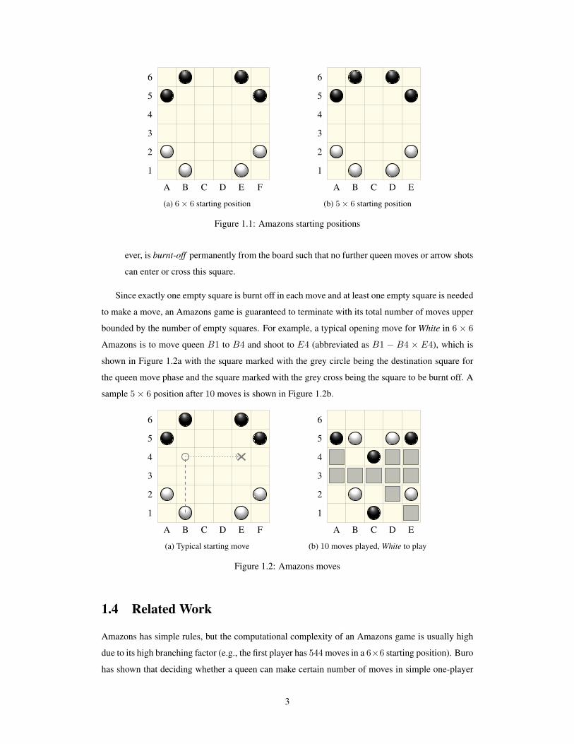
However if G is an infinitesimal, using its stop values overlooks its subtlety. An infinitesimal

has a temperature of 0 (i.e., it is already “cooled down” at temperature 0) and a mean value of 0 (i.e.,

RS(G0) = LS(G0) = 0). Therefore using stop values at 0 as bounds will confuse infinitesimals

with a true integer 0, which is always a second player win. To differentiate infinitesimals from a

true integer 0, the stop values at temperature −1 are used because the stop values of an infinitesimal

at −1 are fixed based on how an infinitesimal compares with 0 [6]. Bounds of infinitesimals are

summarized in Table 2.6. For example, the bounds of ∗, ↑ and ↓ are [-1,1] (see Figure 2.12c for the

illustration), [0,1] and [-1,0], respectively.

Infinitesimal i Bounds of i at temperature −1i > 0 [0,1]i < 0 [-1,0]i || 0 [-1,1]

Table 2.6: Bounds of infinitesimals at temperature −1

23

Chapter 3

Endgame Databases

Based on whether the full board breaks down into subgames in an endgame, endgame databases can

be categorized into full-board or partial-board endgame databases.

A full-board endgame database contains pre-computed thorough analysis of endgame positions

(whose definition is application specific) for a certain game. For a converging game, where the game

complexity reduces as the game progresses, full-board endgame databases are a performance asset

for the game-playing program in reducing its search space by replacing heuristic evaluations with

perfect knowledge [27]. For example, 10-piece endgame databases databases have been successfully

used to solve checkers [28].

For non-converging games such as Havannah, it makes no sense to build full-board endgame

databases [15]. However, if the game board can decompose into independent subgames as in Ama-

zons, partial-board endgame databases can provide the perfect information for the subgames and

they can also be used regardless of the original board size. For example, Tegos has built and used

partial-board endgame database to enhance his Amazons playing program Antiope [32].

Our Amazons endgame databases are built separately for the three different area types as in

Section 2.3.3. In this chapter, we mainly discuss the building of the blocker territory databases used

in our solver. Since databases of the other two types have been built and used before, we only give

the differences in our implementation.

3.1 Building Blocker Territory Databases

3.1.1 Database Format

There are three parameters for a single blocker territory database: the number of normal queens,

the number of blockers and the size of the blocker territory. The three parameters are stored in

the beginning of a database file. The number of entries is also stored to avoid dynamic memory

allocation when loading the database.

Each entry in a database file stores the position of the blocker territory, its value and the cor-

responding best move for achieving its value. The position of a blocker territory is computed by

24

representing each square with a single character from top-left to bottom-right in a row-major fash-

ion, using “E” for empty squares, “B” for Black queens, “A” for arrows and “O” for blockers. The

value of a blocker territory is the maximum number of moves achievable in this position stored as

an integer (see Appendix A). For example, Figure 3.1 shows a 3 × 3 Black blocker territory with 2

blockers A2 and C1 and 1 normal queen A1 and its corresponding entry in the database.

A B C

1

2

3

Position Value Best MoveEEEOAEBAO 4 10758697

Figure 3.1: Blocker Territory Database Entry Format

3.1.2 Building Process

The computational technique used to generate the blocker territory databases is retrograde analy-

sis. Also known as backward induction, retrograde analysis starts by generating terminal positions

whose values are known statically. It then computes positions that lead to a terminal position directly

by doing a 1-ply lookup. After this, positions that are 2-ply away from the terminal positions can

also be generated by a 1-ply lookup, and so on. This process is repeated until either some stopping

criteria (such as the memory limit) or the beginning of the game is reached. Retrograde analysis has

been successfully applied for generating endgame databases [28] and even for completely solving

non-trivial games [26].

Retrograde analysis cannot be applied directly in generating a blocker territory database due to

the presence of blockers. A blocker can also move in a blocker territory, but in order to prevent the

opponent from getting into this territory, it must always shoot back to its origin square. This property

is called the blocker constraint. After its move, a blocker turns into a normal queen and can move

freely thereafter. The possibility of a blocker turning into a normal queen makes the generation

of a blocker territory database dependent on positions that are not part of the database. Therefore,

we need to resolve the dependencies by building potentially needed positions prior to building the

blocker territory database itself.

To be more specific, the positions in a blocker territory database of size w × h with B blockers,

Q normal queens andE = w×h−B−Q empty squares depend on positions of the same size with b

(0 ≤ b ≤ B) blockers, correspondinglyQ+B−b normal queens and e (0 ≤ e ≤ E−B+b) empty

squares. For example, Figure 3.2 shows that the 3 × 3 blocker territory database with 2 blockers

and 1 normal queen depends on 3× 3 positions with 1 blocker, 2 normal queens and up to 5 empty

25

squares and 3× 3 positions with 0 blockers, 3 normal queens and up to 4 empty squares.

3× 3, B = 2, Q = 1, E = 6

3× 3, B = 1, Q = 2, 0 ≤ E ≤ 5 3× 3, B = 0, Q = 3, 0 ≤ E ≤ 4

Figure 3.2: Blocker territory database dependencies example

After the dependencies are built, a regular retrograde analysis process can be applied directly by

generating all positions of size w × h with B blockers and Q normal queens with e (0 ≤ e ≤ E)

empty squares. The building process is given in function RetroBT in Algorithm 2. Function

NewDatabase returns a newly constructed database whose entries have the format as stated in Sec-

tion 3.1.1. Function BlockerTerritoryGenerator iterates through all valid blocker territories

given the width, height, number of normal queens, number of blockers and number of empty squares

of these positions.

Algorithm 2 Blocker Territory Retrograde Analysis

function RetroBT(w, h, B, Q)dependencies← NewDatabase()toBuilt← NewDatabase()E← w× h− B− Q

. Dependencies Handlingfor b = 0 to B− 1 do

MaxDepE← E− B + b

q← Q + B− b

for e = 0 to MaxDepE dofor all position← BlockerTerritoryGenerator(w, h, q, b, e) do

dependencies.Add(position)end for

end forend for

. Retrograde Analysisfor e = 0 to E do

for all position← BlockerTerritoryGenerator(w, h, Q, B, e) dotoBuilt.Add(position)

end forend forreturn toBuilt

end function

3.2 Reducing Databases

The databases built right after the retrograde analysis process are too big to be used effectively.

To reduce the size of the databases generated, we prune out the positions that are redundant (Sec-

tion 3.2.1) and trade time for memory by storing only the normal form of a position (Section 3.2.2).

By pruning out the redundant positions and storing only the normal form of a position, the reduction

26

rates of the blocker territory databases are shown in the last column of Table B.3 in Appendix B.

3.2.1 Redundant Positions

During retrograde analysis, some generated positions, while necessary for the building process, are

redundant once the computation is done. These positions are simply pruned out before the database

is stored on disk. Redundant positions can be classified into two categories:

1. Positions that do not span the full area

For example, when building a 2 × 3 blocker territory database with only 1 blocker, we will

generate the position in Figure 3.3a during retrograde analysis. This position is necessary dur-

ing the building process since it is reachable from other positions (e.g., Figure 3.3b). However,

it is redundant for the final database since all the squares in the top row in this position are

burnt-off and this position will be looked up in the 2× 2 databases instead.

2. Positions that are not 8-connected

For example, the position in Figure 3.3c is also a reachable position from position Figure 3.3b

in the building process. After building, it is removed from the 2× 3 blocker territory database

and it will be looked up in a 1× 2 database.

A B

1

2

3

(a) Does not span the fullarea. Redundant.

A B

1

2

3

(b) Potential parent

A B

1

2

3

(c) Not 8-connected.Redundant

Figure 3.3: Redundant positions

3.2.2 Transformation Detection and Normal Form

A group of different-looking positions might be structurally equivalent due to geometric transfor-

mations. An arbitrary number of rigid transformations (reflection, rotation and translation) can be

applied to a position without changing its structure. For a position in the Amazons databases, we

need to consider 3 transformations: reflection against the x-axis (ref-x), reflection against the y-axis

(ref-x) and 90◦ counterclockwise rotation (rot-c90). The 8 unique combination sequences (named

t0 to t7) of these 3 transformations are shown in Table 3.1. t0 means no transformations are applied.

For example in Figure 3.4, assuming p0 is the original position, p0 through p7 are positions after

applying corresponding transformation sequences t0 to t7.

27

t0 : none t4 : rot-c90t1 : ref-x t5 : rot-c90→ ref-xt2 : ref-y t6 : rot-c90→ ref-yt3 : ref-x→ ref-x t7 : rot-c90→ ref-x→ ref-y

Table 3.1: Transformation Sequences

A B C123

A B C123

A B C123

A B C123

A B C123

A B C123

A B C123

A B C123

ref-x ref-x

ref-y ref-y

p0 p1

p2 p3

p4p5

p6p7

rot-c90

Figure 3.4: Transformations

For a group of structurally equivalent positions, keeping one of them in the database is sufficient.

Define the code of a square on an Amazons position to be “B” for Black queens, “W” for White

queens, “A” for arrows, “E” for empty squares and “O” for blockers. Define the signature of an

Amazons position to be the concatenation of the codes of all its squares from its lower-left corner

to its upper-right corner in a row-major fashion (i.e., first row from left to right then second row

from left to right, etc.). We define the normal form of a m× n position, amongst all its 8 possible

transformations, as:

• the one with the lexicographically smallest signature if m = n, and

• the “slimmer” one (i.e., its width is smaller than its height) with the lexicographically smallest

signature if m 6= n.

In the databases, only these normal forms are stored.

For example, the signatures of positions p0 to p7 in Figure 3.4 are shown in Table 3.2. Therefore,

the normal form of positions p0 to p7 is p2.

28

p0 : EEWBEEEAE p4 : EBEAEEEEWp1 : WEEEEBEAE p5 : EBEEEAWEEp2 : EAEBEEEEW p6 : EEWAEEEBEp3 : EXEEEBWEE p7 : WEEEEAEBE

Table 3.2: Signatures

3.3 Databases UsedSimple territory databases

The simple territory databases we built are similar to the ones Tegos used [32]. However, we used

the blocker territory database entry format for the simple territory databases rather than line segment

graphs as in Tegos’ implementation. Using line segment graphs can potentially further reduce the

size of the database but it also takes longer to query a position because a position has to be converted

into such a graph for query, which is more complex than computing its normal form. We computed

48 simple territory databases and their statistics are summarized in Table B.1 in Appendix B.

Active area databases

For active area databases, we used the implementation by Enzenberger which is part of the Arrow

code base. 1 For each entry, we store the position as in the territory databases and its corresponding

thermograph. The active area databases are not built with the blocker constraint. Therefore they

cannot be used to query a remaining active area when blocker territories are partitioned out in an

improved partition. Table B.2 in Appendix B shows the statistics of the active area databases. We

computed 87 active areas in total but only 86 of them are used in solving. The active area database

of size 3 × 6 with 2 queens for each color is not used because it is too large (43433015 entries) to

be loaded quickly enough. The loading time of all the active area databases with this database is 12

hours and it is 45 minutes without. Such 3 × 6 areas does not occur too often in solving the 5 × 6

board (see Table C.4 in Appendix C).

Blocker territory databases

Statistics on the 106 blocker territory databases we built are summarized in Table B.3 in Appendix B.

1The Arrow code base contains C++ source code for building Amazons playing and solving programs. It was built andmaintained by Martin Muller since 2002. Enzenberger was a major contributor. The Arrow code base may go open source inthe future [22].

29

Chapter 4

Improving Area and Global Bounds

In this chapter, we discuss how the bounds of different types of areas are computed. In Section 4.1,

we show how bounds each type of area are initialized and computed with the heuristics or local

search. In Section 4.2, we discuss how the bounds of an area of each type are computed with the

databases. Finally in Section 4.3, we show how to combine bounds computed in different ways into

global bounds for the entire board.

4.1 Computing Bounds by Heuristics

4.1.1 Simple Territory

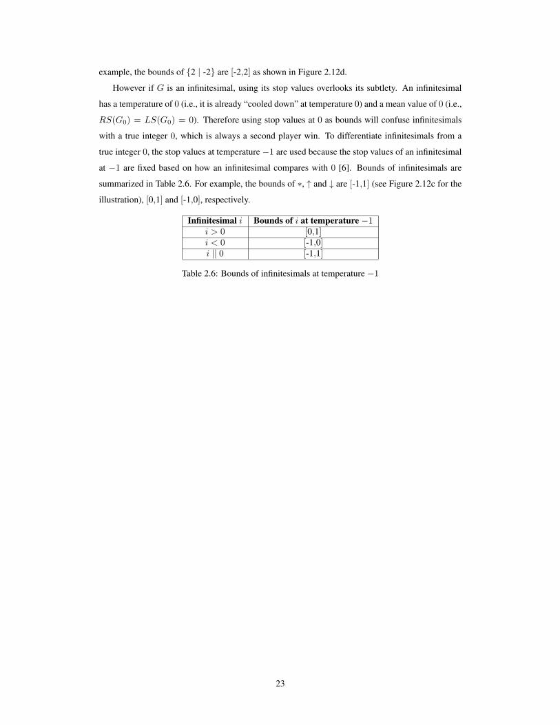
The bounds of a Black simple territory with v empty squares are initialized to [0, v]. The bounds of

a White simple territory with v empty squares are initialized to [−v, 0]. These initial bounds simply

indicate that the opponent cannot move in this area, but are not claiming any moves for the owner.

Since there is no easy way to determine whether a simple territory can be completely filled or not

(see Section 2.3.3), the simple plodding heuristic in solving 5 × 5 is used to quickly compute an

basic lower bound for a simple territory [23]. The plodding heuristic counts the number of moves

a queen in a simple territory can make by greedly making as many plodding moves (moving into a

neighboring square and shooting back) as possible. The lower bound of a simple territory is set to

the sum of the number of plodding moves over all queens in this simple territory where each empty

square is used by at most one queen. With the plodding heuristic, the upper bound always equals to

the number of empty squares in a simple territory.

For example, the bounds of the position shown in Figure 4.1 are [1, 2] since the heuristic can

only make 1 move with this Black queen. Even though this is a defective simple territory and the

maximum number achievable moves is 1, the heuristic can not determine whether the remaining

square is reachable or not.

30

A B

1

2

3

Figure 4.1: Simple territory bounds heuristics, bounds [1, 2]

4.1.2 Blocker Territory

The bounds of a territory are initialized the same way as a simple territory. In filling a blocker

territory, the plodding heuristic has one additional constraint which is to avoid using blockers if

possible.

For example, the position shown in Figure 4.2 is a Black blocker territory with the Black queen

B2 as its blocker. The bounds computed by the heuristic are [1, 3] since the blocker has to shoot

back when it moves, thus blocking its access to other empty squares.

A B C

1

2

3

Figure 4.2: Blocker territory bounds heuristics, bounds [1, 3]

4.1.3 Active Area

The bounds of an active area with v empty squares are initialized to [−v, v]. These crude bounds

can be improved either by static evaluation or by local minimax searches. The static evaluation

improves bounds by quickly identifying safe moves for both players, which is which is rather weak

for large areas but fast enough to be applied to arbitrary positions. The local search, on the other

hand, provides the bounds for an active area by exhaustive minimax search. It is only conducted on

small positions as a complement to the databases, so as not to slow down the solving process.

Static Evaluation

A queen needs at least one adjacent empty square (AES) to make a move. The purpose of static

evaluation is to find out if there are safe (i.e., guaranteed) moves for both players and improve the

bounds according to the following rules:

1. For every Black safe move, the lower bound is increased by 2;

2. For every White safe move, the upper bound is decreased by 2.

31

Each safe move changes the bounds by 2 because one safe move for a player also means one less

move for his opponent. For example, if Black has 2 safe moves and White has 1 in an active area

with v empty points, the improved bounds will be [−v + 4, v − 2].

How many safe moves a queen can make depends on its AES status, the opponent’s queen

distribution and whose turn it is to move next. Muller has shown the following rules for finding safe

moves [23]:

1. A queen with 3 or more AES has a safe move. For example, in Figure 4.3a, Black queen B2

has a safe move because it has 3 AES.

2. A queen with 2 AES such that the opponent cannot block both in one move. For example, the

Black queen B1 in Figure 4.3b has a safe move because it has two AES that the White queen

B2 cannot block in a single move.

3. A queen with 2 AES which the opponent can block in one move has a safe move if and only if

in blocking these two empty squares, the opponent has to open up another AES for the same

queen. For example, in Figure 4.3b, Black queen B1 can take both empty squares in one

move. However in doing so, B1 will be a new AES for the White queen B2, therefore B2

also has a safe move.

4. A queen with 1 AES which the opponent cannot block has a safe move.

A B C

1

2

(a) Black queen B2 has 3 AES[23]

A B C

1

2

(b) Black queen B1 has 2 safeAES

Figure 4.3: Static evaluation Rules

The fourth rule can be improved by taking the original square of the opponent queen which

blocks the single AES into account. For example, in Figure 4.4 the White queen A2 has 1 AES

B2 which the Black queen D2 can block easily by D2 − C3 × B2 as shown in the figure. But in

blocking this AES, Black has to free the White queen D1 it blocked. Therefore, a safe move can be

claimed for the two White queens combined.

The second rule above did take the opponent square into consideration but only for the same

queen with the 2 AES and thus can be improved in a similar fashion. For example, in Figure 4.5, the

White queen D1 has 2 AES and the Black queen A3 can block both by moving to C1 and shooting

to C2. However, in doing this, Black has to open up his original square A3 which has an adjacent

White queen B4. Therefore, White can claim a safe move for D1 and B4 combined.

32

A B C D

1

2

3

Figure 4.4: New static evaluation rule for queens with 1 AES

A B C D

1

2

3

4

Figure 4.5: New static evaluation rule for queens with 2 AES

Muller also pointed out that there are potential dependencies amongst queens [23]. Therefore,

the static evaluation is only performed once at most for each player in an active area . For example,

in Figure 4.6, there are 4 empty squares in the active area (original bounds [−4, 4]) and the Black

queen C1 and both White queens A2 and E2 can find a safe move. However, White cannot claim

two safe moves because it can make only one move if Black moves first by C1−B1×D1. Bounds

of this area are improved only to [−2, 2] due to the dependencies of the White queens.

A B C D E

1

2

3

4

Figure 4.6: Static evaluation dependencies example

Local Search

Bounds of an active area can also be computed by local minimax searches on the fly. To compute the

bounds of an active areaA, two local minimax searches are started onA with Black and White being

the first player respectively. In order to make the search results consistent with the databases, we

search for the number of moves the first player can make more than his opponent. This is achieved

by maintaining a single stack s for a local search. Name the first player to move in the local search

fp, each time fp plays a legal move, +1 is pushed onto s. Each time fp’s opponent plays a legal

move, −1 is pushed onto s. 0 is pushed onto s if the player to move passes. Passes are allowed for

33

both players even if they have other legal moves so as to handle zugzwang positions correctly. The

game is terminated after two consecutive passes.

For example, Figure 4.7a and Figure 4.7b shows the principal variation in the local search of the

position in Figure 2.8 with Black and White being the first player respectively. The stack s when the

search terminates is also shown along with the principal variation.

A B C123

A B C123

1

0

0

(a) Black plays first, search score 1

A B C123

A B C123

A B C123

1

−1

0

0

(b) White plays first, search score 0

Figure 4.7: Local search of Figure 2.8

Let the local search value be vw and vb for White and Black moving first in an active area A

respectively. The bounds of A are set to [−vw, vb]. For example, in Figure 4.7, the bounds are set to

[0, 1] after the local search. For efficiency reasons, local searches are only performed on positions

whose total number of queens and empty squares is less than 9 in the solver.

4.2 Computing Bounds from Databases

4.2.1 Simple Territory Databases

When a Black simple territory is encountered during the search, it is changed to its normal form and

queried against the simple territory database of the corresponding size and queen number. If the

query is successful, its exact value v is returned and the bounds for this territory are set to [v, v].

If it was a White simple territory, the color of the queens is changed to Black (i.e., negate the

game) and the position is queried as a Black simple territory as described above. The return value

is negated after the query succeeded. For example, Figure 4.8 shows a White simple territory of

size 2× 3 with only one queen and its corresponding querying position. Because this is a defective

territory, the query returns a value of 1. Thus the bounds for this White simple territory are [−1,−1].

4.2.2 Active Area Databases

During the search, if an active area is encountered and the number of its Black queens is no less

than the number of its White queens, this active area is first converted to its normal form and then

34

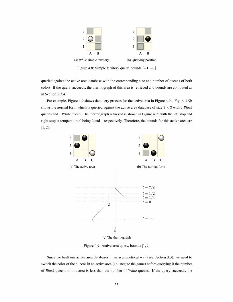
A B

1

2

3

(a) White simple territory

A B

1

2

3

(b) Querying position

Figure 4.8: Simple territory query, bounds [−1,−1]

queried against the active area database with the corresponding size and number of queens of both

colors. If the query succeeds, the thermograph of this area is retrieved and bounds are computed as

in Section 2.3.4.

For example, Figure 4.9 shows the query process for the active area in Figure 4.9a. Figure 4.9b

shows the normal form which is queried against the active area database of size 3× 3 with 2 Black

queens and 1 White queen. The thermograph retrieved is shown in Figure 4.9c with the left stop and

right stop at temperature 0 being 2 and 1 respectively. Therefore, the bounds for this active area are

[1, 2].

A B C

1

2

3

(a) The active area

A B C

1

2

3

(b) The normal form

t = 7/8

t = 1/2t = 1/4t = 0

t = −1

138

3

2

1

(c) The thermograph

Figure 4.9: Active area query, bounds [1, 2]

Since we built our active area databases in an asymmetrical way (see Section 3.3), we need to

switch the color of the queens in an active area (i.e., negate the game) before querying if the number

of Black queens in this area is less than the number of White queens. If the query succeeds, the

35

bounds computed from the thermograph will be negated to account for the color switching.

For example, the position in Figure 4.10 has 2 White queens and 1 Black queen. Therefore the

color of the queens will be switched before the query. The position after the color switching is

identical to Figure 4.9a, thus the query process is the same as in Figure 4.9 except that the resulting

bounds will be negated to [-2,-1].

A B C

1

2

3

Figure 4.10: Active area query with more White than Black queens, bounds [-2,-1]

4.2.3 Blocker Territory Databases

Blocker territories are the result of an improved partition of an active area. Therefore if the original

active area itself is queryable as a whole, there is no need to identify blocker territories within. The

original active area will be queried and processed as described in Section 4.2.2. If an active area

is too large to be queried, an improved partition is performed on it. If no blocker territories can be

partitioned out, then the bounds of this active area are computed as shown in Section 4.1.3.

If an improved partition succeeds, bounds of the resulting blocker territories and active areas are

computed separately. A blocker can be used to improve the bounds of at most one area it is part of.

For example, Figure 4.11 shows a blocker territory (delimited by the red dashed line) with 1 normal

queen A1 and 1 blocker B2. The blocker B2 can either be used to fill the blocker territory or make

moves in the remaining active area.

A B C D

1

2

3

Figure 4.11: Blocker territory with 1 normal queen and 1 blocker

Because neither our active area databases nor local searches consider the blocker constraint,

bounds of the remaining active areas currently are only computed with static evaluations as stated in

Section 4.1.3, with an additional constraint that blockers that are used in other areas must not be used

to find safe moves (either by itself or combined with other queens). Therefore the more blockers

we can spare from using in blocker territories, the better the chances are there for tighter active area

bounds. For example, in Figure 4.11, if the blocker B2 is used in filling the blocker territory, then it

cannot be used in improving the bounds of the remaining active area. The bounds of the remaining

36

active area are therefore [-4,2] since White can find a safe move with 3 AES. However, if the blocker

B2 is used to improve the bounds of the remaining active area, its bounds will be [-2,2] because now

Black can also find a safe move.

Unfortunately, in order to reduce the size of blocker territory databases, we did not store the

information as to which queens are used in filling a blocker territory. Therefore, if we query a

blocker territory directly, we need to assume all its blockers and normal queens are used for filling,

even if it can be filled with a small subset of them. For example, the blocker territory in Figure 4.11

is clearly completely fillable by either the normal queen A1 or the blocker B2. However, if we

queried the blocker territory as is, we have to assume both queens are used in filling it.

Changing the Querying Position

To resolve this problem, we built 3 heuristics for selecting a subset of all the queens in a blocker

territoryB to be in its querying positionB′ to minimize the number of blockers used. However, there

is one drawback for eliminating certain queens in the querying position B′ of a blocker territory B:

if B′ is defective, we are not sure whether B is defective or not. In terms of bounds, bounds(B) =

[u(bounds(B′), e], where e is the number of empty squares in B. Notice that if B′ is non-defective,

B has to be non-defective since this value can be achieved by moving only the queens in B′ while

leaving the other queens untouched. For example, if the blocker C2 is taken out from the blocker

territory in Figure 4.12, then this territory is defective and its bounds are [1, 2].

A B C

1

2

3

4

Figure 4.12: Black territory is defective if the blocker C2 is taken out

The selection process is based on the queens’ types. Algorithm 3 summarizes the queen selection

process with the details explained in the rest of the section.

1. Normal Queens Or Blockers Blocking Dead Active Areas

In a blocker territory, two types of queens are always included in the querying position:

(a) normal queens.

Normal queens are always included because they have no constraints in choosing moves.

They are the best candidates for filling a blocker territory.

(b) blockers that block a dead active area.

Due to the process of building the blocker territory databases, a blocker will always shoot

37

Algorithm 3 Blocker territory queen selection

function BTQueenSelect(bt). bt is a blocker territory

normal← 0

blockDead← 0

blockOne← 0

blockMore← 0

. separate the queens based on their typesfor all q← bt.queens do

if q is a normal queen thennormal.Add(q)

else if q blocks a dead active area thenblockDead.Add(q)

else if q blocks a single territory thenblockOne.Add(q)

elseblockMore.Add(q)

end ifend for

. queens selectionif normal.size > 0 or blockDead.size > 0 then

return normal + blockDead

else if blockOne.size > 0 thenreturn SelectBlockOne(blockOne)

elsereturn SelectBlockMore(blockMore)

end ifend function

38

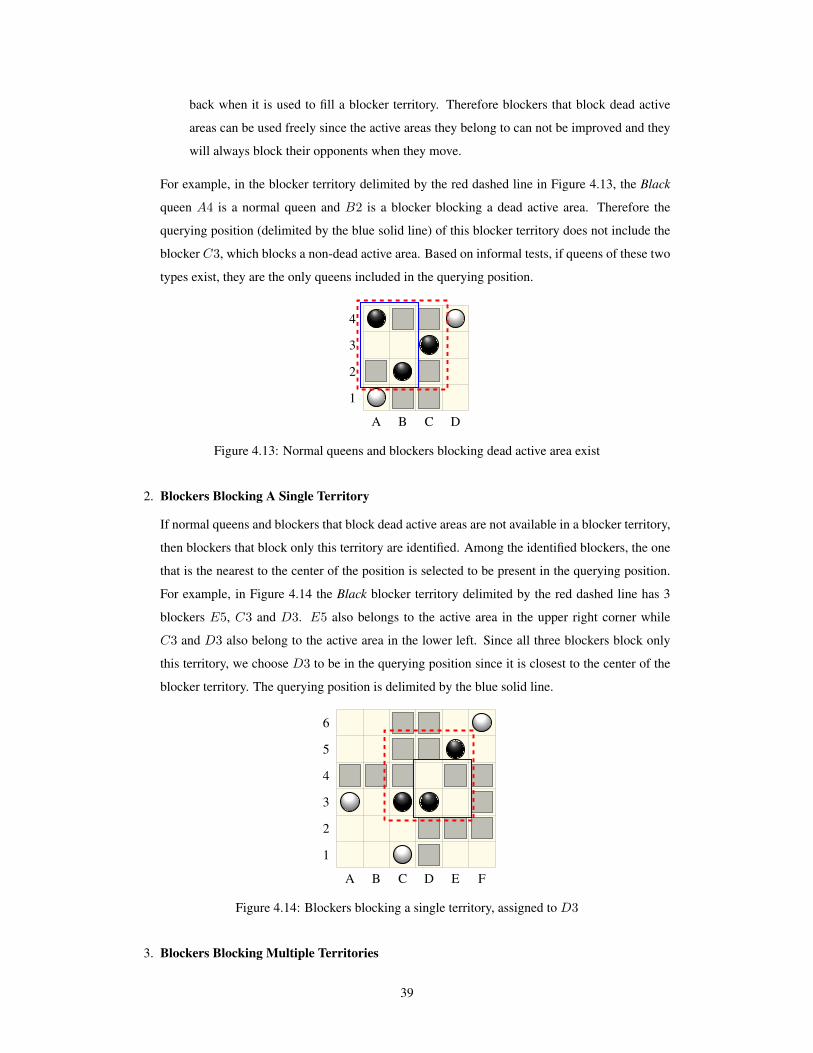
back when it is used to fill a blocker territory. Therefore blockers that block dead active

areas can be used freely since the active areas they belong to can not be improved and they

will always block their opponents when they move.

For example, in the blocker territory delimited by the red dashed line in Figure 4.13, the Black

queen A4 is a normal queen and B2 is a blocker blocking a dead active area. Therefore the

querying position (delimited by the blue solid line) of this blocker territory does not include the

blocker C3, which blocks a non-dead active area. Based on informal tests, if queens of these two

types exist, they are the only queens included in the querying position.

A B C D

1

2

3

4

Figure 4.13: Normal queens and blockers blocking dead active area exist

2. Blockers Blocking A Single Territory

If normal queens and blockers that block dead active areas are not available in a blocker territory,

then blockers that block only this territory are identified. Among the identified blockers, the one

that is the nearest to the center of the position is selected to be present in the querying position.

For example, in Figure 4.14 the Black blocker territory delimited by the red dashed line has 3

blockers E5, C3 and D3. E5 also belongs to the active area in the upper right corner while

C3 and D3 also belong to the active area in the lower left. Since all three blockers block only

this territory, we choose D3 to be in the querying position since it is closest to the center of the

blocker territory. The querying position is delimited by the blue solid line.

A B C D E F

1

2

3

4

5

6

Figure 4.14: Blockers blocking a single territory, assigned to D3

3. Blockers Blocking Multiple Territories

39

Blockers blocking multiple territories are only considered when queens of other types are not

available. If the only queen available in a blocker territory blocks multiple territories, it can only

guarantee the biggest one by walking in it and shooting back to block the opponent. Instead of

computing bounds for each of the blocker territories it blocks, a single bound is computed for

all involved blocker territories combined [23]. Let B be the set of bounds for all the blocker

territories blocked by a common blocker, then the combined bounds are:

[maxb∈B

l(b),∑b∈B

u(b)]

In other words, the combined lower bound is the maximum lower bound in B and the combined

upper bound is the sum of all upper bounds in B.

For example, in Figure 4.15, the Black blocker B2 is blocking two territories (delimited by the

red dashed line) with bounds of [1, 1] and [2, 2] respectively. The combined bounds are therefore

[max(1, 2), (1 + 2)] = [2, 3], which means Black can make at least two moves in these two

blocker territories and could make at most three.

A B C D

1

2

3

Figure 4.15: B2 blocks two territories, combined bounds [2, 3]

If all queens in a blocker territory block multiple territories, we “assign” this territory to the

blocker whose maximum blocker territory (excluding this one) is the smallest. The reason for

such a choice is that this blocker territory should be used to assist the “weakest” blocker to

achieve a better overall bound. For example, in Figure 4.16 the shared Black blocker territory

(delimited by the red dashed line) will be assigned to B3 since it blocks another territory of size

1 and D3 blocks another territory of size 2. The querying position is delimited by the blue solid

line.

A B C D E F

1

2

3

4

5

Figure 4.16: Both Black blockers block multiple territories, assigned to B3

40

4.3 Combining Bounds

After a game position is partitioned into areas, and bounds of each area are computed, we need

to combine all the area bounds into a single global bound and try to determine the winner of this

position based on the rules in Section 2.3.1.

The overall structure of the bounds combination process is summarized in Algorithm 4. For

simple territories (computed by heuristics or from the databases), blocker territories (computed by

heuristics or from the databases, assuming blockers blocking multiple blocker territories are handled

properly as stated in Section 4.2.3) and active areas computed by static evaluation and local search,

the combining process is a simple bounds summation. For active areas computed from the databases

however, the combining process is more complex because we have better knowledge of these games

and can achieve better bounds. The handling of these games is explained in the next two subsections.

Algorithm 4 Area bounds combination

function AreasCombine(areas)infAreas← EmptySet

hotAreas← EmptySet

globalBounds← [0, 0]. sum up everything besides infinitesimals and hot games

for all a← areas doif a is an infinitesimal then

infAreas.Add(a)else if a is a hot game from the database then

hotAreas.Add(a)else

globalBounds← globalBounds + bounds(a)end if

end for. hot games from the databases handling

globalBounds← HotCombine(globalBounds, hotAreas). infinitesimals handling

globalBounds← InfCombine(globalBounds, infAreas)

return globalBounds

end function

Handling Hot Games From the Databases

In theory, all hot games should be summed to a single game and the bounds of the resulting game

will be used. However, we cannot do this in our current framework with thermographs. Instead, we

improve the global bounds by assuming the next player will move in the hot game with the widest

bounds. The widest bounds is the bounds whose upper and lower bound have the biggest absolute

difference. Let the widest bounds be bw. If the next player is Black, we add [u(bw), u(bw)] instead

of bw; If the next player is White, we add [l(bw), l(bw)] instead of bw. For example, if the widest

bounds are [−2, 2], then [−2,−2] are added if the next player is White, and [2, 2] are added if the

41

next player is Black.

We can add the widest bounds from the next player’s point of view because this value is guar-

anteed by its thermograph and the next player can achieve such a value by moving in the area that

provides the widest bounds. Adding the widest bounds uses the next player’s privilege of moving

first, which can be used at most once during the entire bounds combining process. All other bounds

besides the widest are simply added to the global bounds.

The entire process for handling hot games from the databases is shown in Algorithm 5. Function

NextPlayer will return the next player and function RevokeToMovePrivilege marks the next

player’s privilege of moving first as used.

Algorithm 5 Hot games from the databases bounds combination

function HotCombine(globalBounds, hotAreas)maxRange← 0

widest← NULL

. find the area with the widest boundsfor all a← hotAreas do

range← u(bounds(a))− l(bounds(a))if range > maxRange then

maxRange← range

widest← a

end ifend for

. add on the widest in favor of the next playerif NextPlayer() is Black then

globalBounds← globalBounds + [u(bounds(widest)), u(bounds(widest))]else

globalBounds← globalBounds + [l(bounds(widest)), l(bounds(widest))]end ifRevokeToMovePrivilege()

. add on the rest of the boundsfor all a← hotAreas do

if a is not widest thenglobalBounds← globalBounds + bounds(a)

end ifend for

return globalBoundsend function

Handling Infinitesimals

Infinitesimals are strictly less than any positive number and greater than any negative number. There-

fore if the bounds of all other areas combined (called oBounds) are in one player’s favor (i.e.,

l(oBounds) > 0 or u(oBounds) < 0), the winner is determined and there is no need to add the

bounds of any infinitesimals. If oBounds does not favor any player, bounds of infinitesimals have

to be added on.

Bounds of infinitesimals are handled in two parts according to whether an infinitesimal is a ∗.

42

1. ∗s are counted and are combined into a single variable starBounds as follows:

starBounds =

{[− 1, 1] if there is an odd number of ∗s[0, 0] if there is an even number of ∗s

2. All other infinitesimals are summed together to produce a single variable iBounds as follows:

iBounds =

[0, 1] all other infinitesimals are positive[− 1, 0] all other infinitesimals are negative[− 1, 1] otherwise

If the next player’s privilege of moving first was not used in the hot game handling phase, it can

also be combined with the infinitesimals to provide one free move for the next player. The criteria

for this free move is shown below and the process is summarized in Algorithm 6.

• Black as the next player has a free move if

– no other infinitesimals exist and there is an odd number of ∗s;

– all other infinitesimals are positive and there is an even number of ∗s.

• White as the next player has a free move if

– no other infinitesimals exist and there is an odd number of ∗s;

– all other infinitesimals are negative and there is an even number of ∗s.

Algorithm 6 Decide whether infinitesimals can provide a free move for the next player

function HasInfMove(starBounds, iBounds). odd number of stars and no other infinitesimals

if iBounds = [0, 0] and starBounds = [−1, 1] thenreturn true

end if. odd number of stars and no other infinitesimals

if iBounds 6= [0, 0] and starBounds = [0, 0] thenif NextPlayer() is Black and l(iBounds) ≥ 0 then

return trueelse if NextPlayer() is White and u(iBounds) ≤ 0 then

return trueend if

end if. otherwise

return falseend function

If the next player’s privilege of moving first is used in the hot game handling phase or the in-

finitesimals are not strong enough to provide a move, starBounds and iBounds are then combined

and added to oBounds. This entire infinitesimals handling process is shown in Algorithm 7. Func-

tion HasToMovePrivilege returns true if the next player’s privilege of moving first is not used yet

and false otherwise.

43

Algorithm 7 Infinitesimal bounds combination

function InfCombine(oBounds, infAreas). inifinitesimal bounds are not necessary

if l(oBounds) > 0 or u(oBounds) < 0 thenreturn oBounds

end if. count the stars and sum the rest

starCount← 0

iBounds← [0, 0]for all a← infAreas do

if a is ∗ thenstarCount← starCount + 1

elseiBounds← [min(l(iBounds), l(bounds(a))),max(u(iBounds), u(bounds(a)))]

end ifend for

. sum the starsstarBounds← NULL

if starCount is odd thenstarBounds← [−1,+1]

elsestarBounds← [0, 0]

end if. check if the next player has a free move

if HasToMovePrivilege() and HasInfMove(starBounds, iBounds) thenif NextPlayer() is Black then

oBounds← oBounds + [1, 1]else

oBounds← oBounds + [−1,−1]end ifRevokeToMovePrivilege()

elseiBounds← [min(l(starBounds), l(iBounds)),max(u(starBounds), u(iBounds))]oBounds← oBounds + iBounds

end if

return oBoundsend function

44

4.3.1 Board Evaluation Examples

Examples shown in this section are endgame positions from self-play games by the program Arrow

2.1 (a UCT player) given 500 seconds per game.

A ∗Win

A B C D E F

1

2

3

4

5

6

AreaA

AreaB AreaC

AreaD

Figure 4.17: 19 moves played, Black to move, global bounds [1, 1]

Figure 4.17 shows a 6 × 6 Amazons endgame position after 19 moves have been played and

there are 9 empty squares left. The board is partitioned into 4 active areas and all the areas can be

looked up in the databases. Area A is the infinitesimal ∗ and Areas B, C and D are all the integer

0. Therefore, the global bounds after summing up everything besides hot games and infinitesimals

are still [0, 0]. The infinitesimal handling phase will recognize the ∗ and use the to-move privilege

to claim a free move for Black from the ∗. The overall global bounds therefore are [1, 1] and Black

can win the game by moving in Area A, leaving the rest of the board (a 0 game) to White.

Without the databases, all areas would be locally searched with the bounds of Area A being

[−1, 1] and the bounds of AreasB,C andD being [0, 0]. The global bounds therefore are [−1,−1]+

[0, 0] + [0, 0] + [0, 0] = [−1, 1]. Because all the results comes from the local search, we cannot use

Black’s privilege of moving next to claim a move for him. Therefore the winner of this position

cannot be determined yet.

A New Static Evaluation & Infinitesimal Win

Figure 4.18 shows a 6×6 Amazons endgame position after 18 moves have been played and there are

10 empty squares left. Area A is a 2 × 6 active area with 2 White queens and 1 Black queen which

can be queried from the database. The query result of AreaA is−4+ i where i is some infinitesimal

that is confused with 0 (i is actually a ∗, but the database information is not strong enough to prove

it). Area B is an active area with 4 empty squares wherein a safe move can be found for White with

the two White queens C4 and E1 combined with the new static evaluation rules. Black has a safe

move in AreaB using the old static evaluation rule, therefore the bounds of AreaB are [−2, 2]. Area

C is a Black blocker territory with bounds of [1, 1]. Without the infinitesimal i, the global bounds

45

A B C D E F

1

2

3

4

5

6 AreaA

AreaB

AreaC

Figure 4.18: 18 moves played, White to move, global bounds [−5,−1]

are [−4,−4] + [−2, 2] + [1, 1] = [−5,−1]. Because the upper bound already indicates a win for

White, there is no need to add on the infinitesimal part. This position therefore is a White win.

Without the databases, Area A would be partitioned into a White blocker territory (delimited by

red dashed line in Figure 4.18) with bounds of [−4,−4]. The remaining active area has 1 empty

square and neither player can find a safe move (bounds [−1, 1]). Therefore, the global bounds are

[−4,−4] + [−1, 1] + [−2, 2] + [1, 1] = [−6, 0]. Since it is White to move, the winner cannot be

determined yet.

A Local Search Win

A B C D E F

1

2

3

4

5

6 AreaAAreaB

AreaC

Figure 4.19: 21 moves played, White to move, global bounds [1, 3]

Figure 4.19 shows a 6 × 6 Amazons endgame position after 21 moves have been played and

there are 6 empty squares left. Area B is looked up in the active databases as a ∗. Area C is looked

up in the simple territory databases with its bounds being [1, 1]. Area A has a size of 3 × 6 so it

is too large to be in the database. However, Area A can be locally searched with its bounds being

[0, 2]. The global bounds without the infinitesimal therefore are [0, 2] + [1, 1] = [1, 3]. Since the

lower bound is greater than 0, Black wins this position and there is no need to add the infinitesimal

bounds.

Without the databases, Areas B and C will be evaluated as [−1, 1] and [1, 1] respectively. The

46

global bounds then are [0, 2] + [1, 1] + [−1, 1] = [0, 4]. Because it is White to move and the lower

bound is 0, this position is still evaluated as a Black win.

However, without the local search, Area A will be evaluated as [−2, 2] because both players can

find a safe move in Area A. The global bounds then will be [−2, 2] + [1, 1] + [−1, 1] = [−2, 4]. The

winner of the position cannot be determined based on these bounds.

47

Chapter 5

Experiments and Results

5.1 Area Evolution

Figure 5.1, 5.2, 5.3 and 5.4 illustrates how different types of areas evolve during game play on 5×5,

5 × 6, 6 × 5 and 6 × 6 boards respectively. For each figure, the statistics are averaged over 100

self-play games by program Arrow 2.1 (a UCT player) given 500 seconds per game. In each figure,

subfigure (a) shows a summary of all the areas and subfigure (b) shows statistics of only the active

areas in more detail. The legends in these figures are explained in Table 5.1.

Legend Meaningtotal the sum of all types of areas

simp-t: q simple territories queried from the databasessimp-t: h simple territories computed by heuristics

blk-t: q blocker territories queried from the databasesblk-t: h blocker territories computed by heuristics

active: q active areas queried from the databasesactive: h active areas computed by heuristicsactive: s active areas computed by local searches

infi infinitesimals in active: qnumber numbers in active: q

hot hot games in active: q

Table 5.1: Legends of Figure 5.1 to 5.4

These figures clearly illustrate how an Amazons board decomposes into separate areas as the

game progresses. For all board sizes, the number of simple and blocker territories computed by

heuristics is either 0 or very close to 0. This means that almost all territories occurring during game

play fall in the databases. The number of active areas that are locally searched is also close to 0

and it happens only towards the end of the game. Among the queried active areas, numbers and

infinitesimals are predominant towards the end of the game.

Several interesting data points in the figures are compiled in Table 5.2. The name of the points

are:

• avl: the average length of the games.

48

(a) Summary

(b) Active areas only

Figure 5.1: Area evolution on 5× 5 board

49

(a) Summary

(b) Active areas only

Figure 5.2: Area evolution on 5× 6 board

50

(a) Summary

(b) Active areas only

Figure 5.3: Area evolution on 6× 5 board

51

(a) Summary

(b) Active areas only

Figure 5.4: Area evolution on 6× 6 board

52

• a1l: the average length of the opening of the games where the number of active areas com-

puted by heuristics is within 2% of 1. This data point measures the average length where the

entire board is the predominant active area.

• tip: the point where the total number of areas starts increasing. Smaller areas start emerging

at this point. This point is usually close to bip, since the players try to block off parts of the

board as their blocker territories at this stage.

• tdp: the point where the total number of areas starts decreasing. This point usually indicates

that the game is entering the endgame phase when the areas are gradually filled up and become

dead areas.

• tpv: the peak value of the total number of areas.

• sip: the point where the number of simple territories starts increasing. sip is always later

than bip. This indicates strong play from both players because usually no queens should be

completely isolated from the rest of the board at this stage.

• sdp: the point where the number of simple territories starts decreasing. sdp always comes

after bdp. This point usually indicates when the game enters the territory-filling stage.

• bip: the point where the number of blocker territories starts increasing.

• bdp: the point where the number of blocker territories starts decreasing.

• sbp: the point where the number of simple territories exceeds the number of blocker territo-

ries.

• aip: the point where the number of queried active areas starts increasing. This is the earliest

point where the active area databases start being helpful.

• adp: the point where the number of queried active areas starts decreasing.

• ahp: the point where the number of queried active areas exceeds the number of active areas

computed by the heuristics. After this point, most of the active areas on board can be queried

from the database. Solving positions hereafter is usually easy.

53

Data Point 5× 5 5× 6 6× 5 6× 6avl 15.98 21.08 21.60 26.54a1l 9 10 10 15tip 4 9 5 7tdp 12 18 17 19tpv 2.73 2.2 2.38 3.46sip 8 12 11 9sdp 16 21 20 24bip 4 11 5 6bdp 8 14 14 19sbp 14 15 20 20aip 9 9 8 9adp 15 16 17 18ahp 13 11 15 19

Table 5.2: Interesting data points in area evolution

5.2 Solving Test Cases

We have two solvers for solving Amazons: ab (a minimax based solver) and dfpn (a DFPN solver).

To gauge the performance of the solvers and the databases, the test set from [23] is used. This test

set contains three test games named f1, f2 and f3, which were played by an early version of our

Amazons playing program Arrow against a human expert [23]. f1 and f2 were played on the 5× 5

board and f3 was played on the 6 × 6 board. All three game files can be found at [21]. Test cases

in the test set are positions selected from these games. Configurations of the solvers are shown in

Table 5.3. All endgame databases as described in Section 3.3 are used in these tests. The time limit

is 10000 seconds per test case for all solvers.

Solver Name Hash Table Othersab 225

ab db 225 endgame databasesdfpn 222

dfpn db 222 endgame databases

Table 5.3: Solver configurations – test set

The search results for f1, f2 and f3 are shown in Figure 5.5, 5.6 and 5.7 respectively. For each

picture, the horizontal axis is labelled with the test case number and the difficulty of the test cases

increases from left to right. The vertical axis shows the number of nodes searched to solve a test

case in the logarithm scale. Even with a hash table of 18 of the size of that used by ab, dfpn searches

fewer nodes than ab, sometimes by orders of magnitude, in all the test cases except for position 2 in

f3. The statistics for ab on position 10 in f3 is missing because it did not finish the search within

time limit. In these test cases, dfpn db never searches more nodes than dfpn. Sometimes dfpn db

can reduce the number of nodes needed by dfpn by an order of magnitude.

54

Figure 5.5: Search result of f1

Figure 5.6: Search result of f2

55

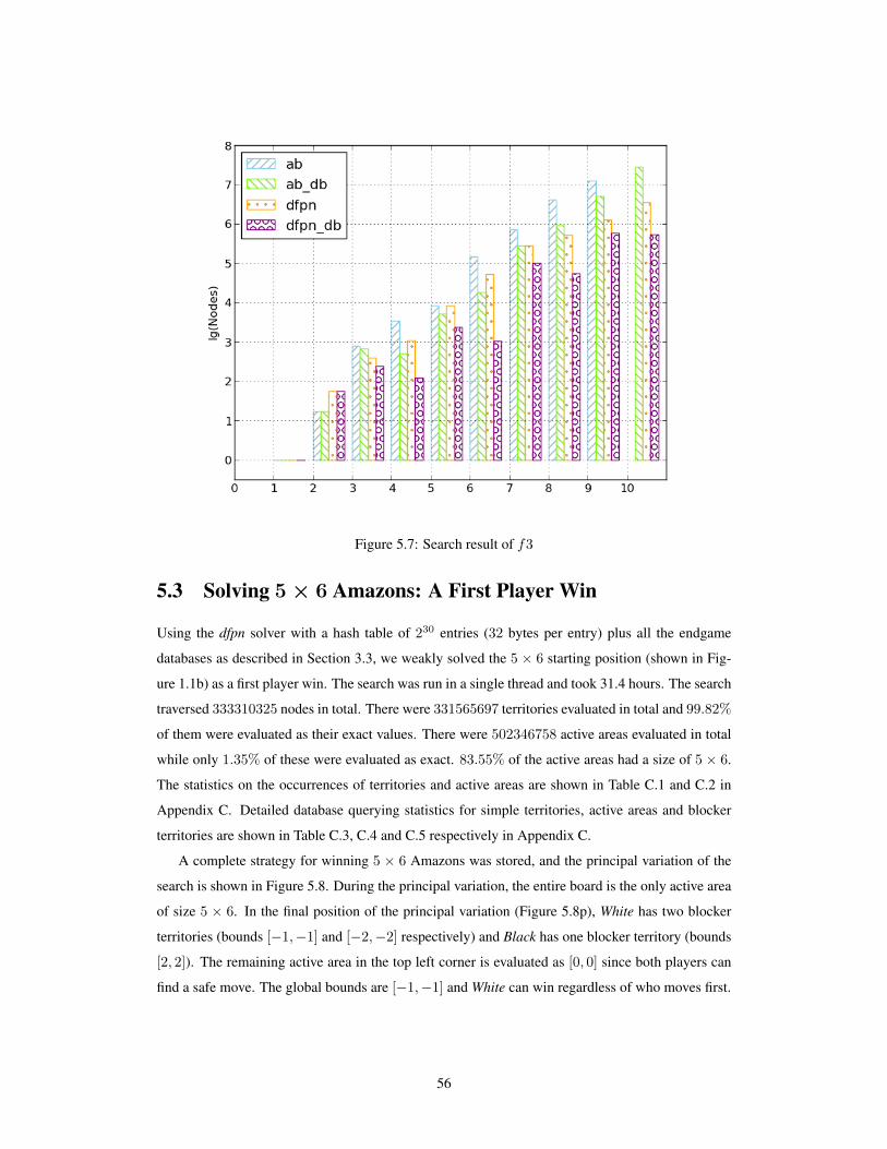
Figure 5.7: Search result of f3

5.3 Solving 5 × 6 Amazons: A First Player Win

Using the dfpn solver with a hash table of 230 entries (32 bytes per entry) plus all the endgame

databases as described in Section 3.3, we weakly solved the 5 × 6 starting position (shown in Fig-

ure 1.1b) as a first player win. The search was run in a single thread and took 31.4 hours. The search

traversed 333310325 nodes in total. There were 331565697 territories evaluated in total and 99.82%

of them were evaluated as their exact values. There were 502346758 active areas evaluated in total

while only 1.35% of these were evaluated as exact. 83.55% of the active areas had a size of 5 × 6.

The statistics on the occurrences of territories and active areas are shown in Table C.1 and C.2 in

Appendix C. Detailed database querying statistics for simple territories, active areas and blocker

territories are shown in Table C.3, C.4 and C.5 respectively in Appendix C.

A complete strategy for winning 5 × 6 Amazons was stored, and the principal variation of the

search is shown in Figure 5.8. During the principal variation, the entire board is the only active area

of size 5 × 6. In the final position of the principal variation (Figure 5.8p), White has two blocker

territories (bounds [−1,−1] and [−2,−2] respectively) and Black has one blocker territory (bounds

[2, 2]). The remaining active area in the top left corner is evaluated as [0, 0] since both players can

find a safe move. The global bounds are [−1,−1] and White can win regardless of who moves first.

56

A B C D E123456

(a) B1−B4×D4

A B C D E123456

(b) E5− E3× E6

A B C D E123456

(c) D1−D3×D2

A B C D E123456

(d) A5−A3× C1

A B C D E123456

(e) B4−B5×B2

A B C D E123456

(f) A3−B3×D1

A B C D E123456

(g) D3− C2× C4

A B C D E123456

(h) E3−D3× E3

A B C D E123456

(i) B5− C5× E5

A B C D E123456

(j) B3−A3×B3

A B C D E123456

(k) C2− C3× C2

A B C D E123456

(l) B6−B5×B4

A B C D E123456

(m) C5−B6× C5

A B C D E123456

(n) D6− C6×D6

A B C D E123456

(o) B6−A5×B6

A B C D E123456

(p) White wins

Figure 5.8: 5× 6 board principal variation, White moves first and wins

57

5.4 Solving Early 6 × 5 and 6 × 6 Positions

In order to evaluate the solver’s performance on bigger boards, we also solved some early 6× 5 and

6× 6 positions. For each board size, we generated 100 self-play games with program Arrow 2.1 (a

UCT player). Then we started solving each game from the end of the game with 500 seconds per

position until we ran into the first position that exceeds the time limit. The solver we used was dfpn

with all the databases and a hash table of 222 entries.

# Moves # Solved # Avg Node22 74 1.0021 88 1.0020 98 1.0119 100 1.1118 100 4.2817 100 5.3716 100 38.3815 100 21.2514 100 446.3913 100 566.0312 100 5386.5211 100 6978.6210 100 65212.439 100 83433.018 99 1339502.877 59 623908.366 25 700953.925 16 548137.81

Table 5.4: Solving early 6× 5 positions

Table 5.4 and 5.5 show the results on 6× 5 and 6× 6 boards respectively. Within 500 seconds,

99 out of the 100 6×5 games are solved after 8 moves, and 95 out of the 100 6×6 games are solved

after 10 moves. These results suggest that to solve 6 × 5 or 6 × 6 Amazons, a forward search of

at most 8 or 10 plies is needed before the current solver can solve a position reasonably fast. The

number of games solved beyond these points decreases rapidly. For example, 16 games are solved

after 5 moves on the 6× 5 board, and only 2 games are solved after 7 moves on the 6× 6 board.

58

# Moves # Solved # Avg Node28 24 1.0027 61 1.0026 76 1.0025 94 1.0024 99 1.0023 100 1.0022 100 1.0321 100 3.2120 100 4.9019 100 16.0818 100 32.7217 100 155.0116 100 318.3915 100 1432.0814 100 2778.0913 100 17043.1212 100 41942.3111 97 193850.1910 95 501987.989 77 685108.748 53 634355.267 2 2548.00

Table 5.5: Solving early 6× 6 positions

59

Chapter 6

Future Work

6.1 Parallel Computing

All the solvers we are using now are single-threaded. However, as the problems we are trying

to solve get larger, it makes more sense to have a multi-threaded/distributed solver with a master

process/machine generating unsolved nodes and a farm of slave processes/machines actually solving

them.

6.2 Summing Games

Storing the thermographs of games is cheaper than storing their full combinatorial-game-theoretical

values. However, it also restricts us from employing the full power of the theory and the databases

since thermographs do not support game addition [6]. For example, Figure 6.1 shows the position

that is one move before the position shown in Figure 4.17. Areas A, C and D are the same as in

Figure 4.17 and they are ∗, 0 and 0 respectively. Area B is actually a ∗, however from the query

result, we can only tell that Area B is an infinitesimal that is confused with 0. Therefore we cannot

use the next player’s moving privilege to provide a free move and the global bounds are [−1, 1]. If

we could sum up the games, this position is 0 and White loses.

A B C D E F

1

2

3

4

5

6

AreaA

AreaB AreaC

AreaD

Figure 6.1: White to move, all areas queried, cannot sum

60

6.3 Database Improvements

Currently the territory databases store both defective and non-defective positions because because

the search engines used require a best move in each non-terminal position. However, this is not

necessary because once the exact value v of a position is known, playing the best move in it will lead

to a position of v − 1. Therefore, we can prune out the non-defective positions from the databases

and the best move field for the defective entries. This will reduce the size of the territory database

drastically as is evident from Table B.1 in Appendix B.

Active area databases can also be built with the blocker constraint such that the remaining active

areas in an improved partition can also be queried.

6.4 Other Improvements

• Local search improvements. Currently, the local search module is not using the databases

and it does not consider the blocker constraint. Both of these can be added on to achieve better

local search results.

• Proof number initialization. The proof and disproof numbers of a newly created node can

be initialized to indicate how easy or hard it is expected to solve a node [25]. Combined with

a decent evaluation function, this could achieve better search results.

• Area caching. Caching search results of areas that are not in the databases but arise frequently

in the search can potentially give the solver a performance boost.

• Search unknown areas only. If the perfect information on most of the areas is known, it

might make sense to restrict the global search to only the unknown areas.

61

Bibliography

[1] M. Albert, R. Nowakowski, and D. Wolfe. Lessons in Play. A K Peters, Ltd., 2007.

[2] L.V. Allis. Searching for Solutions in Games and Artificial Intelligence. PhD thesis, Universityof Limburg, 1994.

[3] L.V. Allis and M.P.H. Huntjens. Go-Moku solved by new search techniques. ComputationalIntelligence, 12(1):7–23, 1996.

[4] L.V. Allis and P.N.A. Schoo. Qubic solved again. Heuristic Programming in Artificial Intelli-gence, 3(9):192–204, 1992.

[5] L.V. Allis, M. van der Meulen, and H.J. van den Herik. Proof-number search. ArtificialIntelligence, 66(1):91 – 124, 1994.

[6] E.R. Berlekamp. The economist’s view of combinatorial games. In Games of No Chance:Combinatorial Games at MSRI, pages 365–405. University Press, 1996.

[7] E.R. Berlekamp. Sums of N × 2 Amazons. ”Lecture Notes – Monograph Series”, 35:pp.1–34, 2000.

[8] E.R. Berlekamp, J.H. Conway, and R.K. Guy. Winning Ways for Your Mathematical Plays.Academic Press, 1982.

[9] M. Buro. Takeshi Murakami vs Logistello. In ICGA, volume 20, pages 189–193, 1997.

[10] M. Buro. Simple Amazons endgames and their connection to Hamilton circuits in cubic sub-grid graphs. In Computers and Games Conference, pages 250–261. Springer, 2000.

[11] J.H. Conway. On Numbers and Games. Academic Press, 2000.

[12] E.D. Demaine. Playing games with algorithms: Algorithmic combinatorial game theory. InProc. 26th Symp. on Math Found. in Comp. Sci., Lect. Notes in Comp. Sci., Springer-Verlag,pages 18–32. Springer, 2001.

[13] D. Du and P.M. Pardalos. Minimax and Applications. Kluwer Academic Publishers, 1995.

[14] M. Enzenberger. Smartgame library documentation. http://fuego.sourceforge.net/fuego-doc-1.1/smartgame-doc/index.html. Accessed on Oct 26, 2012.

[15] T. Ewalds. Playing and solving Havannah. Master’s thesis, University of Alberta, Edmonton,AB, Canada, 2012.

[16] T. Furtak, M. Kiyomi, T. Uno, and M. Buro. Generalized Amazons is PSPACE-complete. InProceedings of the 19th International Joint Conference on Artificial intelligence, IJCAI’05,pages 132–137, San Francisco, CA, USA, 2005. Morgan Kaufmann Publishers Inc.

[17] R. Gasser. Solving Nine Men’s Morris. Computational Intelligence, 12(1):24–41, 1996.

[18] P. Hensgens. A knowledge-based approach of the game of Amazons. Master’s thesis, Univer-siteit Maastricht, Maastricht, The Netherlands, 2001.

[19] J. Kloetzer, H. Iida, and B. Bouzy. The Monte-Carlo approach in Amazons. In Proceedings ofthe Computer Games Workshop, pages 185–192, 2007.

[20] D.E. Knuth and R.W. Moore. An analysis of alpha-beta pruning. Artificial Intelligence,6(4):293 – 326, 1975.

62

[21] M. Muller. Amazons Games Played By Arrow2. http://webdocs.cs.ualberta.ca/˜mmueller/amazons/games. Accessed on Dec 13, 2012.

[22] M. Muller. The Amazons-Playing Program Arrow2. http://webdocs.cs.ualberta.ca/˜mmueller/amazons/arrow.html. Accessed on Nov 14, 2012.

[23] M. Muller. Solving 5 × 5 Amazons. In The 6th Game Programming Workshop (GPW 2001),pages 64–71, 2001.

[24] M. Muller and T. Tegos. Experiments in computer Amazons. In More Games of No Chance,pages 243–260. Cambridge University Press, 2002.

[25] A. Nagai. Df-pn Algorithm for searching AND/OR trees and its applications. PhD thesis,Department of Information Science, University of Tokyo, 2002.

[26] J.W. Romein and H.E. Bal. Awari is solved. Journal of the ICGA, 25:162–165, 2002.

[27] J. Schaeffer, Y. Bjornsson, N. Burch, R. Lake, P. Lu, and S. Sutphen. Building the Checkers10-piece Endgame Databases. In Advances in Computer Games, pages 193–210, 2003.

[28] J. Schaeffer, N. Burch, Y. Bjornsson, A. Kishimoto, M. Muller, R. Lake, P. Lu, and S. Sutphen.Checkers is solved. Science, 317(5844):1518–1522, 2007.

[29] J. Schaeffer and A. Plaat. Kasparov versus Deep Blue: The re-match. ICCA Journal, 20(2):95–101, 1997.

[30] B. Sheppard. World-championship-caliber Scrabble. Artificial Intelligence, 134(1):241–275,2002.

[31] R.G. Snatzke. New results of exhaustive search in the game Amazons. Theoretical ComputerScience, 313(3):499 – 509, 2004.

[32] T. Tegos. Shooting the last arrow. Master’s thesis, University of Alberta, Edmonton, AB,Canada, 2002.

[33] J. Uiterwijk, L.V. Allis, and H.J. van den Herik. A knowledge-based approach to Connect-Four. Heuristic Programming in Artificial Intelligence: The First Computer Olympiad, EllisHorwood, Chichester, pages 113–133, 1989.

[34] H.J. van den Herik, J.W.H.M. Uiterwijk, and J. van Rijswijck. Games solved: now and in thefuture. Artif. Intell., 134(1-2):277–311, January 2002.

63

Appendix A

Database Move Encoding

A move in Amazons is associated with three squares on board: the origin square of the moving queen

(s0), the destination square this queen moves to (s1), and the square where the arrow is shot (s2).

Assuming that the function index() extract the index of a square on an Amazons board, an Amazons

move can be encoded by concatenating the indexes of the three squares as shown in Figure A.1.

index(s0) index(s1) index(s2)

Figure A.1: Move encoding

In our implementation, we used the smartgame library [14] which uses 9 bits for indexing a

single square. Therefore an Amazons move can be encoded in a 32 bit integer.

64

Appendix B

Databases Used

Table B.1: Simple territory database statistics

Size Queens Defective ReducedTotal1× 2 1 0 11× 3 1 0 21× 3 2 0 21× 4 1 0 21× 4 2 0 41× 4 3 0 21× 5 1 0 31× 5 2 0 61× 5 3 0 61× 5 4 0 31× 6 1 0 31× 6 2 0 91× 6 3 0 101× 6 4 0 92× 2 1 0 42× 2 2 0 52× 2 3 0 22× 3 1 2 282× 3 2 0 472× 3 3 0 372× 3 4 0 182× 4 1 0 1062× 4 2 0 2522× 4 3 0 2982× 4 4 0 2332× 5 1 12 4112× 5 2 6 12052× 5 3 0 19982× 5 4 0 21412× 6 1 50 14552× 6 2 0 52712× 6 3 0 110602× 6 4 0 155043× 3 1 4 1943× 3 2 6 446

Continued on next page

65

Table B.1 – continued from previous pageSize Queens Defective ReducedTotal3× 3 3 3 5913× 3 4 1 5003× 4 1 40 32163× 4 2 38 104143× 4 3 54 197983× 4 4 46 250253× 5 1 380 276703× 5 2 353 1130153× 5 3 523 2806683× 5 4 715 4746103× 6 1 3423 2229883× 6 2 3309 11082913× 6 3 4956 3403023

Table B.2: Active area database statistics

Size Black White ReducedTotal1× 3 1 1 31× 4 1 1 61× 4 2 1 61× 5 1 1 101× 5 2 1 161× 5 2 2 161× 5 3 1 101× 6 1 1 151× 6 2 1 301× 6 2 2 481× 6 3 1 301× 6 3 2 301× 6 4 1 152× 2 1 1 62× 2 2 1 42× 3 1 1 842× 3 2 1 1042× 3 2 2 932× 3 3 1 592× 3 3 2 322× 3 4 1 162× 4 1 1 4802× 4 2 1 8942× 4 2 2 13502× 4 3 1 8842× 4 3 2 10002× 4 3 3 5402× 4 4 1 5002× 4 4 2 4202× 4 4 3 1402× 5 1 1 2357

Continued on next page

66

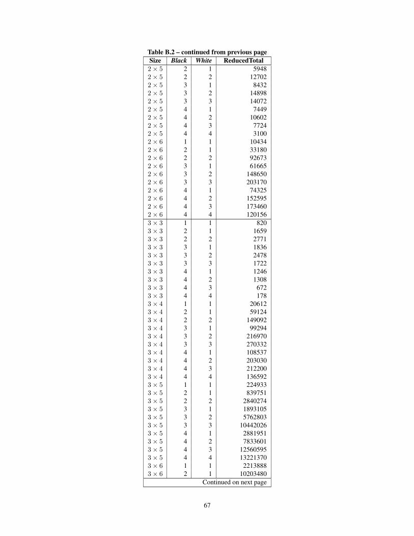
Table B.2 – continued from previous pageSize Black White ReducedTotal2× 5 2 1 59482× 5 2 2 127022× 5 3 1 84322× 5 3 2 148982× 5 3 3 140722× 5 4 1 74492× 5 4 2 106022× 5 4 3 77242× 5 4 4 31002× 6 1 1 104342× 6 2 1 331802× 6 2 2 926732× 6 3 1 616652× 6 3 2 1486502× 6 3 3 2031702× 6 4 1 743252× 6 4 2 1525952× 6 4 3 1734602× 6 4 4 1201563× 3 1 1 8203× 3 2 1 16593× 3 2 2 27713× 3 3 1 18363× 3 3 2 24783× 3 3 3 17223× 3 4 1 12463× 3 4 2 13083× 3 4 3 6723× 3 4 4 1783× 4 1 1 206123× 4 2 1 591243× 4 2 2 1490923× 4 3 1 992943× 4 3 2 2169703× 4 3 3 2703323× 4 4 1 1085373× 4 4 2 2030303× 4 4 3 2122003× 4 4 4 1365923× 5 1 1 2249333× 5 2 1 8397513× 5 2 2 28402743× 5 3 1 18931053× 5 3 2 57628033× 5 3 3 104420263× 5 4 1 28819513× 5 4 2 78336013× 5 4 3 125605953× 5 4 4 132213703× 6 1 1 22138883× 6 2 1 10203480

Continued on next page

67

Table B.2 – continued from previous pageSize Black White ReducedTotal3× 6 2 2 434330154× 4 1 1 2847084× 4 2 1 11213794× 4 2 2 40339944× 4 3 3 17260100

Table B.3: Blocker territory database statistics

Size Normal Queens Blockers ReducedTotal UnreducedTotal ReductionRate1× 2 0 1 1 4 75.00%1× 3 0 1 2 12 83.33%1× 3 0 2 2 6 66.67%1× 3 1 1 3 12 75.00%1× 4 0 1 2 32 93.75%1× 4 0 2 4 24 83.33%1× 4 0 3 2 8 75.00%1× 4 1 1 6 48 87.50%1× 4 1 2 6 24 75.00%1× 4 2 1 6 24 75.00%1× 5 0 1 3 80 96.25%1× 5 0 2 6 80 92.50%1× 5 0 3 6 40 85.00%1× 5 0 4 3 10 70.00%1× 5 1 1 10 160 93.75%1× 5 1 2 16 120 86.67%1× 5 1 3 10 40 75.00%1× 5 2 1 16 120 86.67%1× 5 2 2 16 60 73.33%1× 5 3 1 10 40 75.00%1× 6 0 1 3 192 98.44%1× 6 0 2 9 240 96.25%1× 6 0 3 10 160 93.75%1× 6 0 4 9 60 85.00%1× 6 1 1 15 480 96.88%1× 6 1 2 30 480 93.75%1× 6 1 3 30 240 87.50%1× 6 2 1 30 480 93.75%1× 6 2 2 48 360 86.67%1× 6 3 1 30 240 87.50%2× 2 0 1 4 32 87.50%2× 2 0 2 5 24 79.17%2× 2 0 3 2 8 75.00%2× 2 1 1 6 48 87.50%2× 2 1 2 4 24 83.33%2× 2 2 1 4 24 83.33%2× 3 0 1 28 192 85.42%2× 3 0 2 47 240 80.42%2× 3 0 3 37 160 76.88%

Continued on next page

68

Table B.3 – continued from previous pageSize Normal Queens Blockers ReducedTotal UnreducedTotal ReductionRate2× 3 0 4 18 60 70.00%2× 3 1 1 84 480 82.50%2× 3 1 2 104 480 78.33%2× 3 1 3 59 240 75.42%2× 3 2 1 104 480 78.33%2× 3 2 2 93 360 74.17%2× 3 3 1 59 240 75.42%2× 4 0 1 106 1024 89.65%2× 4 0 2 252 1792 85.94%2× 4 0 3 298 1792 83.37%2× 4 0 4 233 1120 79.20%2× 4 1 1 480 3584 86.61%2× 4 1 2 894 5376 83.37%2× 4 1 3 884 4480 80.27%2× 4 2 1 894 5376 83.37%2× 4 2 2 1350 6720 79.91%2× 4 3 1 884 4480 80.27%2× 5 0 1 411 5120 91.97%2× 5 0 2 1205 11520 89.54%2× 5 0 3 1998 15360 86.99%2× 5 0 4 2141 13440 84.07%2× 5 1 1 2357 23040 89.77%2× 5 1 2 5948 46080 87.09%2× 5 1 3 8432 53760 84.32%2× 5 2 1 5948 46080 87.09%2× 5 2 2 12702 80640 84.25%2× 5 3 1 8432 53760 84.32%2× 6 0 1 1455 24576 94.08%2× 6 0 2 5271 67584 92.20%2× 6 0 3 11060 112640 90.18%2× 6 0 4 15504 126720 87.77%2× 6 1 1 10434 135168 92.28%2× 6 1 2 33180 337920 90.18%2× 6 1 3 61665 506880 87.83%2× 6 2 1 33180 337920 90.18%2× 6 2 2 92673 760320 87.81%2× 6 3 1 61665 506880 87.83%3× 3 0 1 194 2304 91.58%3× 3 0 2 446 4608 90.32%3× 3 0 3 591 5376 89.01%3× 3 0 4 500 4032 87.60%3× 3 1 1 820 9216 91.10%3× 3 1 2 1659 16128 89.71%3× 3 1 3 1836 16128 88.62%3× 3 2 1 1659 16128 89.71%3× 3 2 2 2771 24192 88.55%3× 3 3 1 1836 16128 88.62%3× 4 0 1 3216 24576 86.91%3× 4 0 2 10414 67584 84.59%3× 4 0 3 19798 112640 82.42%3× 4 0 4 25025 126720 80.25%

Continued on next page

69

Table B.3 – continued from previous pageSize Normal Queens Blockers ReducedTotal UnreducedTotal ReductionRate3× 4 1 1 20612 135168 84.75%3× 4 1 2 59124 337920 82.50%3× 4 1 3 99294 506880 80.41%3× 4 2 1 59124 337920 82.50%3× 4 2 2 149092 760320 80.39%3× 4 3 1 99294 506880 80.41%3× 5 0 1 27670 245760 88.74%3× 5 0 2 113015 860160 86.86%3× 5 0 3 280668 1863680 84.94%3× 5 1 1 224933 1720320 86.92%3× 5 1 2 839751 5591040 84.98%3× 5 2 1 839751 5591040 84.98%3× 5 2 2 2840274 16773120 83.07%3× 5 3 1 1893105 11182080 83.07%4× 4 1 1 284708 3932160 92.76%4× 4 2 1 1121379 13762560 91.85%

70

Appendix C

Solving 5 × 6 Amazons Statistics

Table C.1: Territory occurrence statistics in solving 5× 6

Size Simple Territory Blocker Territory Total1× 2 3996342 66003317 69999659(21.11%)1× 3 431227 3911984 4343211(1.31%)1× 4 56579 652646 709225(0.21%)1× 5 22540 14898 37438(0.01%)1× 6 1123 0 1123(0.00%)2× 2 2410303 128333623 130743926(39.43%)2× 3 1306360 71870716 73177076(22.07%)2× 4 125752 17142314 17268066(5.21%)2× 5 155471 7218604 7374075(2.22%)2× 6 5158 28858 34016(0.01%)3× 3 67103 9147174 9214277(2.78%)3× 4 7775 9034087 9041862(2.73%)3× 5 46172 3914078 3960250(1.19%)3× 6 197 46694 46891(0.01%)4× 4 116 1515350 1515466(0.46%)4× 5 3103 3761521 3764624(1.14%)4× 6 1 11430 11431(0.00%)5× 5 46 304022 304068(0.09%)5× 6 169 18844 19013(0.01%)

Grand Total 331565697

Table C.2: Active area occurrence statistics in solving 5× 6

Size Total1× 3 290960(0.06%)1× 4 394287(0.08%)1× 5 104117(0.02%)1× 6 73840(0.01%)2× 2 3078181(0.61%)2× 3 4441047(0.88%)2× 4 2237604(0.45%)

Continued on next page

71

Table C.2 – continued from previous pageSize Total

2× 5 4146069(0.83%)2× 6 1556823(0.31%)3× 3 2081977(0.41%)3× 4 1900830(0.38%)3× 5 9297435(1.85%)3× 6 1968195(0.39%)4× 4 693490(0.14%)4× 5 7454827(1.48%)4× 6 4277333(0.85%)5× 5 38659102(7.70%)5× 6 419690641(83.55%)

Grand Total 502346758

Table C.3: Simple territory query statistics in solving 5× 6

Size Queens Defective Total1× 2 1 0 6352946(46.33%)1× 3 1 0 653973(4.77%)1× 4 1 0 87340(0.64%)1× 5 1 0 23009(0.17%)1× 6 1 0 877(0.01%)2× 2 1 0 3007564(21.93%)2× 3 1 62256 1746394(12.74%)2× 4 1 0 89596(0.65%)2× 5 1 674 19904(0.15%)2× 6 1 33 1758(0.01%)3× 3 1 1185 52895(0.39%)3× 4 1 107 3113(0.02%)3× 5 1 60 3244(0.02%)3× 6 1 2 44(0.00%)1× 3 2 0 54542(0.40%)1× 4 2 0 17011(0.12%)1× 5 2 0 15475(0.11%)1× 6 2 0 988(0.01%)2× 2 2 0 633126(4.62%)2× 3 2 0 475949(3.47%)2× 4 2 0 71671(0.52%)2× 5 2 576 95508(0.70%)2× 6 2 0 4980(0.04%)3× 3 2 518 56980(0.42%)3× 4 2 132 7559(0.06%)3× 5 2 174 24849(0.18%)3× 6 2 0 258(0.00%)1× 4 3 0 574(0.00%)1× 5 3 0 1255(0.01%)2× 2 3 0 5945(0.04%)2× 3 3 0 13267(0.10%)2× 4 3 0 15543(0.11%)

Continued on next page

72

Table C.3 – continued from previous pageSize Queens Defective Total2× 5 3 0 131324(0.96%)2× 6 3 0 61(0.00%)3× 3 3 3 3440(0.03%)3× 4 3 6 1411(0.01%)3× 5 3 16 36755(0.27%)3× 6 3 0 33(0.00%)1× 5 4 0 18(0.00%)2× 3 4 0 12(0.00%)2× 4 4 0 29(0.00%)2× 5 4 0 271(0.00%)3× 3 4 0 16(0.00%)3× 4 4 0 6(0.00%)3× 5 4 0 272(0.00%)

Grand Total 13711785

Table C.4: Active area query statistics in solving 5× 6

Size Black White Integer Fraction Infini Hot Total1× 3 1 1 0 0 57796 0 57796(0.19%)1× 4 1 1 652363 0 103546 3693 759602(2.50%)1× 5 1 1 52944 0 18356 4640 75940(0.25%)1× 6 1 1 19644 0 11681 2599 33924(0.11%)2× 2 1 1 1476705 0 2276449 0 3753154(12.33%)2× 3 1 1 945423 690296 49736 1451068 3136523(10.31%)2× 4 1 1 494522 37613 115026 170818 817979(2.69%)2× 5 1 1 129163 14389 37978 119854 301384(0.99%)2× 6 1 1 75148 8789 16582 46569 147088(0.48%)3× 3 1 1 221722 116982 139296 392293 870293(2.86%)3× 4 1 1 30080 9757 14076 43355 97268(0.32%)3× 5 1 1 26312 3335 12370 55199 97216(0.32%)3× 6 1 1 1911 275 610 3098 5894(0.02%)4× 4 1 1 197 18 40 206 461(0.00%)1× 4 2 1 0 0 25609 0 25609(0.08%)1× 5 2 1 21253 0 32519 2322 56094(0.18%)1× 6 2 1 11562 0 16707 3368 31637(0.10%)2× 2 2 1 0 0 343084 0 343084(1.13%)2× 3 2 1 375999 0 481975 320385 1178359(3.87%)2× 4 2 1 176766 4827 470618 305454 957665(3.15%)2× 5 2 1 447634 122083 444569 1340850 2355136(7.74%)2× 6 2 1 219634 17914 76094 206036 519678(1.71%)3× 3 2 1 229538 66753 245963 395133 937387(3.08%)3× 4 2 1 95312 49962 69402 198467 413143(1.36%)3× 5 2 1 226674 108671 174430 1167457 1677232(5.51%)3× 6 2 1 22904 4128 8773 41000 76805(0.25%)4× 4 2 1 1765 501 892 3027 6185(0.02%)1× 5 2 2 0 0 979 0 979(0.00%)1× 6 2 2 29477 0 18885 133 48495(0.16%)2× 3 2 2 16514 0 33638 1116 51268(0.17%)

Continued on next page

73

Table C.4 – continued from previous pageSize Black White Integer Fraction Infini Hot Total2× 4 2 2 39359 0 63067 16004 118430(0.39%)2× 5 2 2 112077 14453 161228 332096 619854(2.04%)2× 6 2 2 341024 12010 299786 554827 1207647(3.97%)3× 3 2 2 29112 2996 57488 48800 138396(0.45%)3× 4 2 2 57350 12285 78403 106164 254202(0.84%)3× 5 2 2 259645 97032 265001 1072566 1694244(5.57%)4× 4 2 2 5934 2302 7029 13925 29190(0.10%)1× 5 3 1 0 0 636 0 636(0.00%)1× 6 3 1 125 0 72 20 217(0.00%)2× 3 3 1 11141 0 15592 8834 35567(0.12%)2× 4 3 1 15213 44 15449 19563 50269(0.17%)2× 5 3 1 284503 2558 474570 799040 1560671(5.13%)2× 6 3 1 8082 480 9367 15350 33279(0.11%)3× 3 3 1 8961 836 9620 7985 27402(0.09%)3× 4 3 1 13474 1763 17160 21407 53804(0.18%)3× 5 3 1 308278 48305 336749 1787377 2480709(8.15%)1× 6 3 2 0 0 45 0 45(0.00%)2× 3 3 2 0 0 1358 0 1358(0.00%)2× 4 3 2 4047 0 5316 755 10118(0.03%)2× 5 3 2 94765 386 99160 140710 335021(1.10%)2× 6 3 2 66144 657 71693 100049 238543(0.78%)3× 3 3 2 2986 92 4319 2722 10119(0.03%)3× 4 3 2 13224 1138 16842 15968 47172(0.16%)3× 5 3 2 343380 49639 420752 1514668 2328439(7.65%)2× 4 3 3 30 0 50 12 92(0.00%)2× 5 3 3 2971 0 4401 377 7749(0.03%)2× 6 3 3 9383 17 9298 13711 32409(0.11%)3× 3 3 3 84 0 132 43 259(0.00%)3× 4 3 3 820 24 1117 683 2644(0.01%)3× 5 3 3 26333 2054 31207 69956 129550(0.43%)4× 4 3 3 1666 104 1897 1666 5333(0.02%)2× 3 4 1 0 0 14 0 14(0.00%)2× 4 4 1 25 0 57 36 118(0.00%)2× 5 4 1 1175 1 1047 2023 4246(0.01%)2× 6 4 1 7 0 11 25 43(0.00%)3× 3 4 1 53 0 48 24 125(0.00%)3× 4 4 1 181 8 178 168 535(0.00%)3× 5 4 1 14347 1433 12002 61116 88898(0.29%)2× 4 4 2 19 0 10 0 29(0.00%)2× 5 4 2 366 0 578 297 1241(0.00%)2× 6 4 2 502 0 423 497 1422(0.00%)3× 3 4 2 10 0 12 7 29(0.00%)3× 4 4 2 149 9 165 102 425(0.00%)3× 5 4 2 6807 599 6683 29558 43647(0.14%)2× 5 4 3 11 0 9 4 24(0.00%)2× 6 4 3 129 0 143 109 381(0.00%)3× 3 4 3 0 0 1 0 1(0.00%)3× 4 4 3 14 0 15 4 33(0.00%)3× 5 4 3 807 55 858 2183 3903(0.01%)

Grand Total 30427857

74

Table C.5: Blocker territory query statistics in solving 5× 6

Size Normal Queens Blockers Defective Total1× 2 0 1 0 66003307(20.83%)1× 3 0 1 0 2568413(0.81%)1× 4 0 1 0 547037(0.17%)1× 5 0 1 0 13482(0.00%)2× 2 0 1 0 63073574(19.90%)2× 3 0 1 0 18806124(5.93%)2× 4 0 1 0 884067(0.28%)2× 5 0 1 0 163792(0.05%)2× 6 0 1 0 2863(0.00%)3× 3 0 1 7503 1335886(0.42%)3× 4 0 1 259 171016(0.05%)3× 5 0 1 11 10789(0.00%)1× 3 0 2 0 1200956(0.38%)1× 4 0 2 0 37605(0.01%)2× 2 0 2 0 63014400(19.88%)2× 3 0 2 0 45869647(14.47%)2× 4 0 2 0 10461224(3.30%)2× 5 0 2 0 2255803(0.71%)2× 6 0 2 0 17394(0.01%)3× 3 0 2 9381 5475967(1.73%)3× 4 0 2 11479 4629020(1.46%)3× 5 0 2 157 543420(0.17%)2× 2 0 3 0 2026607(0.64%)2× 3 0 3 0 3941361(1.24%)2× 4 0 3 0 3798085(1.20%)2× 5 0 3 0 3597907(1.14%)2× 6 0 3 0 2477(0.00%)3× 3 0 3 896 962657(0.30%)3× 4 0 3 4874 2966685(0.94%)3× 5 0 3 177 2113193(0.67%)2× 3 0 4 0 27715(0.01%)2× 4 0 4 0 97055(0.03%)2× 5 0 4 0 215822(0.07%)2× 6 0 4 0 21(0.00%)3× 3 0 4 17 54383(0.02%)3× 4 0 4 405 142225(0.04%)1× 3 1 1 0 142760(0.05%)1× 4 1 1 0 68001(0.02%)1× 5 1 1 0 1417(0.00%)2× 2 1 1 0 209968(0.07%)2× 3 1 1 0 3071317(0.97%)2× 4 1 1 0 1189582(0.38%)2× 5 1 1 0 253137(0.08%)2× 6 1 1 0 5075(0.00%)3× 3 1 1 6 1076274(0.34%)3× 4 1 1 416 371863(0.12%)3× 5 1 1 6 102742(0.03%)2× 2 1 2 0 9352(0.00%)

Continued on next page

75

Table C.5 – continued from previous pageSize Normal Queens Blockers Defective Total2× 3 1 2 0 122446(0.04%)2× 4 1 2 0 590538(0.19%)2× 5 1 2 0 505803(0.16%)2× 6 1 2 0 856(0.00%)3× 3 1 2 1 192848(0.06%)3× 4 1 2 41 667369(0.21%)3× 5 1 2 10 591251(0.19%)2× 3 1 3 0 402(0.00%)2× 4 1 3 0 4462(0.00%)2× 5 1 3 0 10795(0.00%)2× 6 1 3 0 1(0.00%)3× 3 1 3 0 1398(0.00%)3× 4 1 3 2 41748(0.01%)2× 2 2 1 0 483(0.00%)2× 3 2 1 0 32820(0.01%)2× 4 2 1 0 115491(0.04%)2× 5 2 1 0 210688(0.07%)2× 6 2 1 0 171(0.00%)3× 3 2 1 0 46670(0.01%)3× 4 2 1 0 33964(0.01%)3× 5 2 1 0 131997(0.04%)2× 3 2 2 0 280(0.00%)2× 4 2 2 0 1781(0.00%)2× 5 2 2 0 4515(0.00%)3× 3 2 2 0 703(0.00%)3× 4 2 2 0 9983(0.00%)3× 5 2 2 0 35391(0.01%)2× 3 3 1 0 62(0.00%)2× 4 3 1 0 127(0.00%)2× 5 3 1 0 415(0.00%)3× 3 3 1 0 239(0.00%)3× 4 3 1 0 275(0.00%)3× 5 3 1 0 6050(0.00%)4× 6 3 1 0 5(0.00%)

Grand Total 316895494

76