J.J. Slotine and S.S. Sastry 11

8/12/2019 J.J. Slotine and S.S. Sastry 11

http://slidepdf.com/reader/full/jj-slotine-and-ss-sastry-11 1/56

December 1982LIDS-P-1264

TRACKING CONTROL OF NON-LINEAR SYSTEMS

USING SLIDING SURFACES

WITH APPLICATION TO ROBOT MANIPULATORS

by

J.J. Slotine and S.S. Sastry

Laboratory for Information and Decision Systems

Massachusetts Institute of Technology

Cambridge, MA 02139

Research supported in part by the AFOSR under grant 82-0258 and by the

ONR under grant N00014-82-K-0582 (NR-606-003).



-1-

ABSTRACT

We develop a methodology of feedback control to achieve accurate

tracking in a class of non-linear, time-varying systems in the presence

of disturbances and parameter variations. The methodology uses in its

idealized form piecewise continuous feedback control, resulting in the

state trajectory 'sliding' along a time-varying sliding surface in the

state space. This idealized control law achieves perfect tracking; however,

non-idealities in its implementation result in the generation of an

undesirable high frequency component in the state trajectory. To rectify

this, we show how continuous control laws may be used to approximate the

discontinuous control law to obtain robust tracking to within a prescribed

accuracy and decrease the extent of high frequency signal.

The method is applied to the control of a two-link manipulator

handling variable loads in a flexible manufacturing system environment.

Keywords: Nonlinear control, sliding-mode control, robotics.



-2-

Section 1. Introduction

We present a methodology of feedback control to achieve accurate

tracking for a class of non-linear time-varying systems in the presence of

disturbances and parameter variations. The methodology uses in its idealized

form piecewise continuous feedback control laws, resulting in the state

trajectory 'sliding' along a discontinuity or sliding surface in the

state space. The idealized form of the methodology results in perfect

tracking of the required signals; however certain non-idealities associated

with its implementation cause the trajectory to 'chatter' along the sliding

surface, resulting in the generation of an undesirable high frequency

component in the state trajectory. Not only is the high frequency component

undesirable in itself, but also it may excite high-frequency dynamics

associated with the control system which have been neglected in the course

of modelling. To rectify this situation, we show how continuous control

laws, which approximate in a suitable sense the discontinuous control law,

may be used to obtain tracking to within a prescribed accuracy which is

robust to disturbance signals and parameter variations. At the same time

the continuous control laws decrease the extent of unwanted high-frequency

signals.

The basic concept we use is that of sliding mode control. This has

been studied in great detail in the Soviet literature (see [7], [8] and refer-

ences contained therein), where it has been used to robustly stabilize a class

of non-linear systems. The basic mathematical idea comes from Fillipov [1]:

consider a piecewise continuous differential equation, with the right hand side

discontinuous across a hypersurface. If the trajectories of the differential

equation off the discontinuity surface point towards the discontinuity surface,

it is intuitively plausible that trajectories that start on the discontinuity



-3-

uxrface stay on (slide along) the discontinuity surface -the 'sliding surface'. This

in turn, imposes certain constraints on their dynamics. Further, even if the

right hand side is perturbed, these contraints on the dynamics on the sliding

surface remain the same, so long as the perturbed equation has trajectories

pointing towards the sliding surface (and of course, the sliding surface

is itself not perturbed). By a suitable choice of sliding surface, piece-

wise continuous control law and class of non-linear systems under investiga-

tion,we obtain instances in which the dynamics of the state trajectory

on the sliding surface are completely specified by the constraint that it

stay on the sliding surface. These dynamics are in turn insensitive to

parameter variations in the dynamics of the sliding surface for the same

reasons as those noted above. The shortcomings of the methodology developed

so far in the literature are as follows:

(i) There is a'reaching' phase in which the trajectories starting

from a given initial condition off the sliding surface tend towards the

sliding surface. The trajectories in this phase are sensitive to parameter

variations. Further, convergence to the sliding surface may only be

asymptotic, so that the benefits of sliding mode control cannot be realized.

The literature [10, 12] suggests alleviating these difficulties by the use

of high gain feedback to speed-up the reaching phase. This has the usual

drawbacks associated with high gain feedback - extreme sensitivity to

unmodelled dynamics, actuator saturation, etc. The problem is compounded

in the multi-input case, when the 'hierarchical control' methodology of

[7] is applied. In this method, one starts with a nested chain of sliding

surfaces and derives control laws for a particular sliding surface on the



-4-

assumption that the trajectory actually lies in the intersection of all

preceding sliding surfaces. Since convergence to each sliding surface is

only asymptotic,this may be an invalid assumption.

(ii) Unavoidable small imperfections in switching between control

laws at the discontinuity surface result in the trajectory chattering rather

than sliding along the switching surface. This will in turn excite high-

frequency unmodelled dynamics in the plant.

We remove these drawbacks by developing and using the concept of a

time-varying sliding surface in the state space. We also use time-varying

surfaces to discuss application of our methodology to tracking rather than

stabilization problems. Further, by approximating the discontinuous control

law by a continuous one,we trade off accuracy in tracking against the

generation of high frequency chattering in the state trajectory. The

layout of the paper is as follows:

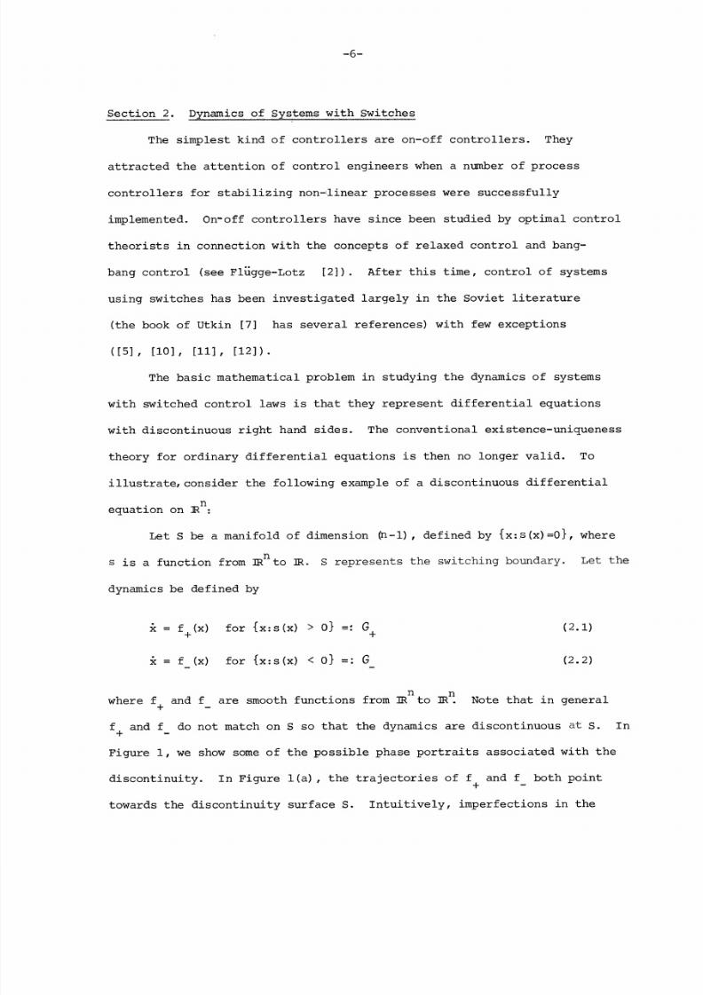
In Section 2, we review results on the dynamics of systems with

switches. We use basic results of Fillipov [1] on solution concepts for

discontinuous differential equations to define a solution concept for

piecewise continuous dynamical systems with the surface of discontinuity

varying with time (time-varying sliding surfaces).

Section 3 illustrates in the simple instance of time-varying linear

systems our methodology of sliding mode control for robust tracking of

specified signals.

In Section 4, we extend the previous results to a class of non-linear,

time-varying systems. Using discontinuous control,we obtain perfect



-5-

tracking in the presence of disturbances and parameter variations. Section

5 modifies the framework of Section 4 to obtain continuous control laws

which approximate the discontinuous control laws of Section 4. We trade

off tracking accuracy for a smaller component of high-frequency signal.

Section 6 describes the applications of our methodology to the

control of a two-link manipulator. We believe our methodology has

important applications to the problems of controlling robots handling

variable loads in a flexible manufacturing system environment. In Section

7 we briefly indicate areas of further research.





-7-

x) )f+ (x)

S S

a) b)

(c)

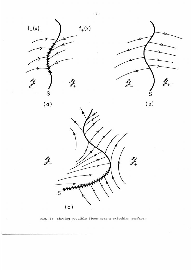
Fig. 1: Showing possible flows near a switching surface.



-8-

switching mechanism should then cause the state trajectory to cross S

infinitely many times or 'chatter' along the surface (as suggested by the

jagged line in the figure). In Figure l(b), the trajectories of f+ and f

both point away from S. It would seem that initial conditions at S would

follow either trajectories of f+ or f (which one, specifically,appears

to be ambiguous) and be repelled from S. In Figure l(c), we have a

combination of circumstances represented in Figures l(a) and l(b), as well

as a region of S in which f_ points towards S and f+ away from it.

One way of regularizing the system description (2.1), (2.2)

consistent with intuition is to assume that (2.1), (2.2) are the degenerate

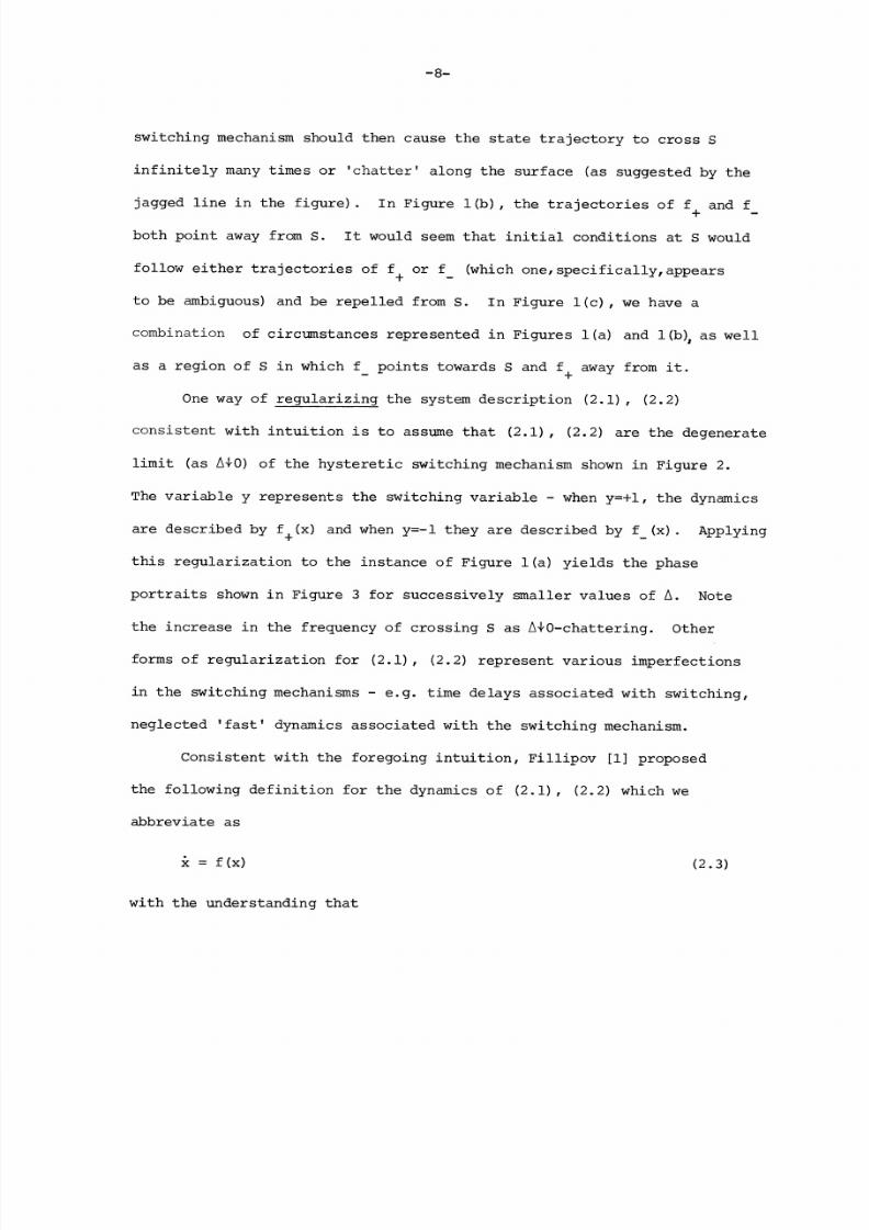
limit (as A+O) of the hysteretic switching mechanism shown in Figure 2.

The variable y represents the switching variable - when y=+l, the dynamics

are described by f+(x) and when y=-l they are described by f_ (x). Applying

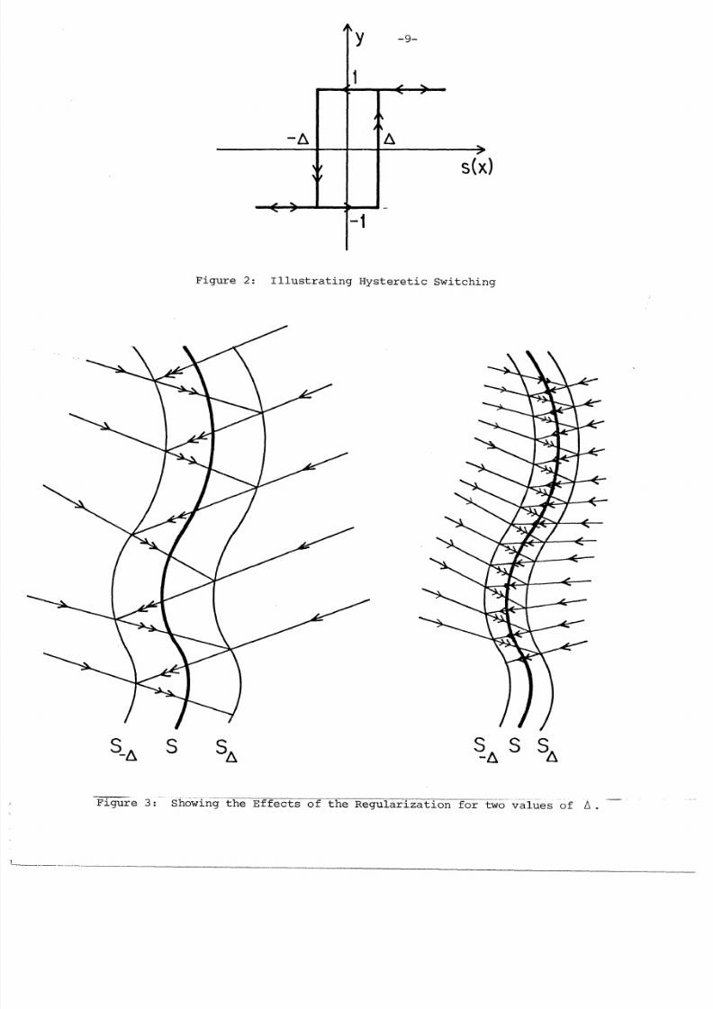
this regularization to the instance of Figure l(a) yields the phase

portraits shown in Figure 3 for successively smaller values of A. Note

the increase in the frequency of crossing S as A+0-chattering. Other

forms of regularization for (2.1), (2.2) represent various imperfections

in the switching mechanisms - e.g. time delays associated with switching,

neglected 'fast' dynamics associated with the switching mechanism.

Consistent with the foregoing intuition, Fillipov [1] proposed

the following definition for the dynamics of (2.1), (2.2) which we

abbreviate as

x = f(x) (2.3)

with the understanding that



- Y -9-

-At ~ s x)i-1

Figure 2: Illustrating Hysteretic Switching

Shwn S SSa S S

Figure 3: Showing the Effects of the Regularization for two values of A



-10-

f(x) = f+(x) for x e G+ , and

f(x) = f (x) for x e G

Definition (Solution Concept for discontinuous differential equations)

An absolutely continuous function x(t): [0,T] + IRnis a solution of

(2.3) if for almost all t G [0,T]

dxe 0 n Cont f(B(x(t),6) - N) (2.4)dt 6>0 N

where B(x(t),6) is a ball of radius 6 centered at x(t),and the intersection

is taken over all sets N of zero measure (Conv refers to the convex

hull of a set).

Remarks (1) The definition (2.4) allows us to exclude sets of zero

measure, such as S, on which f(x) is not defined.

(2) The definition (2.4) is quite general - it includes more general

classes of discontinuous differential equations than those with a piece-

wise continuous right hand side, which are the systems of interest to

us.

We now study the application of the definition to our system (2.3):

Denote by A+(x) (or _ x)) the rate of change of s(x) along the trajectory

of f (x) (or f x)), i.e.

A+(x) = a s(x) . f+(x) for x e G+

X (x) = - s(X) f (x) for x e Gax

Since s(x), f+(x), f_ (x) are all smooth functions of x, both

A (x ) = lim. A(x)+ x-*x*



and

X (x*) = lim A (x)

x+x*

can be defined for x* e S.

Then, in the instance that X+(x*) < 0 and X (x*) > 0 (the situation

of Figure l(a)), it may be shown that for x* C S, definition(2.4) yields

(Lemma 3 of [1]) that

x* = f0(x*) (2.5)

X (x*) X x* )

where f0(x*) (x*) + f (x*) (2.6)X (x*) -X (x*) A+ (x*) -X x* )

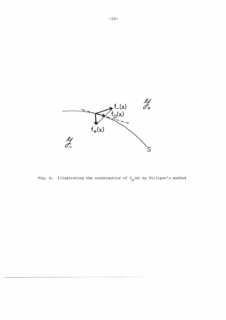
Note that s(x*).fo(x*) = 0 (see the construction of Figure 4) so that

the trajectory slides along S once it hits S (this is referred to as the

sliding mode). This is consistent with the intuition of the regularization

of Figure 3 which suggests that in the limit that A+0, the chattering

becomes infinitely rapid andof infinitesimally small amplitude - f0(x*)

then is the resultant averaging of the chattering. Note also that f0(x*)

is a convex combination of f+(x*) and f_ (x*).

Further, X+(x*) < 0 implies that X+(x) < 0 for x e G+ f B(x*,6),

where B(x*, 6) is a 6 neighbourhood of x* - similarly for X_(x*) < 0.

The conditions

A (x) < 0 for x e B(x*, 6) G+

X (x) > 0 for x e B(x*, 6) n G

maybe combined as



-12-

f_ x)

f+ x)

Fig. 4: Illustrating the construction of f0(x) by Fillipov's method



-13-

d 2-s (x) < 0 for x e B(x*, ) - (2.7)

d 2with the understanding that s (x) is evaluated along the trajectories of

f (x) in G ,and along those of f (x) in G_ . The condition (2.7) is referred+ + - _

to as the local sliding condition, since it is sufficient to guarantee that

trajectories originating from initial conditions close to S converge to

S and then slide along S.

If in fact we have that s(x) is a proper function and

dt s (x) < -~(Isl) for x e R n (2.8)

where i is some function of Class K (see e.g. Vidyasagar [9]), then all

inital conditions lying off S will be attracted to S (global sliding

condition) and then slide along S. Of course, the convergence to S in

either case may only be asymptotic, so that the chattering behavior

indicated in Figure l(a) may not be observed in finite time. Equations

(2.7)or(2.8) however guarantee that trajectories originating on S will

remain on S.

Further, in the instance that X+(x*) > 0 and X (x*) > 0, Lemma 9

of [1] establishes that the trajectory of definition (2.1) has only x*

in common with S and goes from G to G+ through x*. Similar conclusions

hold for the case when X_ (x*), X (x*) < 0.

Fillipov proves existence and continuability of solutions theorems

for his solution concept (Theorems 4 and 5). For the uniqueness of

solutions, some further conditions are required. For our case of a piece-

wise continuous differential equationFillipov's Theorem 14 states that

so long as at least one of the two inequalities



-14-

X (x*) >, X+(x*) < 0 (2.9)

is satisfied at each point x* e S, the system (2.3) has a unique solution

(in the sense of Definition(2.4))for a given initial condition. Further,

the solution depends continuously on initial conditions.

Remark: The requirement that one of the two inequalities of (2.9) hold

rules out the ambiguous situation of Figure 1(b), for instance.

The preceding development was for the stationary case, i.e., s,

f+, f were not explicitly functions of time. For the case when s, f+

and f are functions of x and t, it may be seen that the development

generalizes as follows: define the sliding surface M 0 in (x,t) space

as

M_ = {(x;t):s(x;t) = 0} C IRn+l

Define, also

X (x;t) s(x;t) + s(x;t) ' f (x;t)

In the instance that X (x*;t) < 0 and X (x*; t) > O,formulae completely

analogous to (2.5), (2.6) may be obtained. One way of observing this

is to note that the time-varying case can be converted to the form

studied earlier by augmenting the state space with the t-variable and

augmenting the dynamicswith t=l. We may then state that the (x,t)

trajectory slides along the manifold M0 once it reaches MO .

As before, the uniqueness theorem is also valid so long as at

least one of the two inequalities



-15-

X (x*; t*) > O, A+(x*; t*) < 0 (2.10)

is satisfied for each (x*; t*) e M O. As before, +(x*, t*) < 0 implies

that A+(x;t) < 0 for (x;t) e B((x*; t*), 6) M where M+ = {(x;t):s(x;t) > 0}.

Also, X (x*; t*) > 0 implies that A+(x;t) > 0 for (x;t) e G((x*;t*),6)OM

where M = {(x;t): s(x;t) < 01, and the conditions for sliding along the

surface M0 , namely,

X (x;t) > 0 for (x;t) e B((x*;t*), 6)n M

A+(x;t) < 0 for (x;t) e B((x*;t*), 6) n M

may be combined as

d 2

dt s (x;t) < 0 for (x;t) e B((x*;t*), 6) - M0 2.11)

d 2with the understanding that -d s (x;t) isevaluated along trajectories of

f+(x;t) in M+,and along those of f (x;t) in M_. (2.11) is the local sliding

condition.

If we have that b(x,t) is a proper function and

dt SxI- M0 2.12)

for some function k of class K , then all initial conditions lying off

M0 will be attracted to M 0 and slide along MO . As before, the convergence

to M0 may only be asymptotic so that the sliding mode is not observed

in finite time.

By a minor abuse of notation ,we shall denote by S(t) sections of the

manifold M 0 in the state space JR i.e

S(t) = {x e IRn: s x;t) = 0} (2.13)



-16-

(2.13) has the interpretation of a time-varying sliding surface in the

state space. Then, we may rewrite the local sliding condition (2.7) for

the time-varying case as

d 2ds (x;t) < 0 for x e B(x*, 6) - S(t) (2.14)dt

and the global sliding condition (2.12) for the time-varying case as

d s (x;t) < -_(is(x;t) ) for x e IRn- S(t) (2.15)

at time t.

In this section, we assumed that f and f were smooth functions

(smooth means Cr

for some r). However, as it may be seen from [1], all

of our conclusions hold when the functions f+ and f- are merely Lipschitz

continuous.



-17-

Section 3. Sliding Mode Control for a Class of Single-Input Linear Time

Varying Systems

We illustrate some of the robustness and parameter insensitivity

properties of discontinuous or sliding mode control for the case of an

nth order linear time-varying control system with a single input.

Specifically, consider:

(n) (n-l) (n-2)x(n) + a (t) n 1) + a (t)x +...+ a (t)xl = u (3.1)

n-l 1 n-2 1 0 1

The control problem to be solved is to get xl(t) to track a specified

trajectory xdl (t): a given smooth function from IR+to IR. Some conditions

need to be imposed on xdl (t) to match the initial conditions of (3.1):

(n-l) T nprecisely, define the vectors x(t) = [x (t), l( t),...,x (t) e IR

and x (t) = [Xlt), k (t),. (n-., (t) T e IRn . For simplicity, wed dl' dl(t) dl

denote x( t) and Xl (kt) by x+ t) and Xd (t) respectively. We de-denotex

k )(dl+l dk+l

fine the tracking error x(t) as

x t) = x(t) - xd(t ) = [xl t) . .,t) ]T1 n

Then, we assume that the tracking error is zero at time zero:

x(O) = 0 (3.2)

Further, equations (3.1) can be written in controllable canonical form

as

0L n x + u = :A(t)x +Bu (3.3)



-18-

thNow, we assume that the nr-- derivative of xdl is bounded by a constant v:

Ixd,n+l(t) < v v t e R (3.4)

and define the time-varying sliding surface S(t) by

s(x;t) = C x(t) = 0 (3.5)

where C is a row vector of the form [Cl,..., c , 1]. If the control

u(t) could be chosen so as to keep the trajectory on s(x;t) = 0 we would

have from (3.5) that

(n-l) n-2 (i) (n-l) n2 (i)

x1 + Z ci+lx = Xdl + Y Ci+lxdl (3.6)

i=O i=O

(i) (i)Since the initial conditions on x) match those on the xdl we would then

1 d

have from standard uniqueness results for ordinary differential equations

that

x(t) - x (t) Vt e IR .

Thus, it remains only to choose control u(t) so as to cause the(x;t)trajectory

to slide along the surface specified by (3.5), i.e. a control u that

satisfies condition (2.12) with

S(t): = {x:Cx = O}

We will choose control u of the form

n-1Tu = 3 (x) - x + Z ki (x;t)x i - k sgn s

i=li+l n

n-l

[tl(X),... , n(x) lx + Z ki(x;t)xi+l- k sgn s 37)i=l

sgn s is defined as:

sgn s = 1 for s > 0; sgn s = -1 for s < 0



-19-

with k.(x), i=l,...,n suitably selected. Using (3.7) we obtain

n n-l

l s (x;t) = Z (a(x) - ai l(t))xi s + (c +k. (x;t)) +.sdt 1i=- 1 i=li +1

-S xdn+l- knl (3.8)

To get (3.8) to satisfy (3.12), we use

i(x) := < a. (t) for x.-s > 0 and allt, i=l,...,n (3.9)

i(x) := > a (t) for xi..s < 0 and all t,i=l,...,n (3.10)

k (x;t)::= k. < -C. for x. s > 0 and all t, i=l,... ,n-11 1 -- 1 l~l'

(3.11)

k.(x;t): = k > -c. for Xi+l < 0 and all t, i=l,...,n-1

(3.12)

and

k > v (3.13)n

with the understanding that when c.=O for some i, we will discard the

corresponding term k (x;t)xi+l in the control law. Note that the control

law defined by (3.7), (3.9)-(3.13) has discontinuities at

1 Jxi=O i=l,...,n xj=O j=2,...,n

and

s(x;t) := Cx = 0

It is easy to verify, however, that the (possibly time-varying) discontinuity

surfaces {x:x. = 0}, and {x:xi = 01 are not sliding surfaces since for

each x* on any one of these surfaces, we have



-20-

X+(x*;t*) = X (x*,t*) 0 for all t* (3.14)

so that trajectories may be continued through them. Further, from (3.8),

we have an equation of the form(2.15), namely:

1dt s (x;t) < -(k -v)Is(x;t)J (3.15)

2 dt n

for all t and x e {x : s 0, xi.0, 9ji0; i=l,... ,n, j=2,... ,n}. From

equations (3.14), (3.15) we may conclude that {x:s(x;t) = 01 is a sliding

surface, that is, all trajectories starting off the sliding surface ,

converge to it.Further, all state trajectories starting on the surface

stay on it for all future time. Thus the feedback control defined by

equations (3.7), (3.9)-(3.13) yields x(t) = xd (t).

We now exhibit the parameter insensitivity of the sliding mode control

law. Assume that a. t) is not known exactly - rather, only bounds on its1

magnitude ai, yi are known, i.e.,

i < a (t) < i=O,... ,n- (3.16)

Then (3.9) is satisfied for all t if

B < a1 i-1

for i=l,...,nand

> 1

and the resultant control law (3.7), (3.9)-(3.13) yields x(t) = xd (t).

Robustness of the control law to disturbances follows along similar

lines: consider an additive disturbance vector of the form d(x;t) =

[O,...,O,d (x,t)]T where1



-21-

n

Idl x;t)I < Z xilx 60

i=l

The form of the disturbance follows from the fact that equations (3.3)

are a state space realization of (3.1). Then the control law of the form

(3.8) will yield x(t) = xd(t) so long as

1-- 1-1 i

i=l,... ,n (3.17)

.>

i-+

6.1--

and

k > v + 60 . (3.18)

Conditions (3.11), (3.12) on k1 ,..., kn1 do not need to be modified to

reject this disturbance. We remark here, that from (3.17) we have that

83 - P + i- - a. + 26 i=l,...,n_ 1-- 1 i 1 1

As expected, the minimum discontinuity in the control u (measuredby

i- Si for i=l,...,n, ki ki for j=l,.. ,n-1, and2kn) required to reject

disturbances and parameter variation increases with the strength of the

disturbance to be rejected and the range of parameter variation in the

dynamics of the system.

We next comment on the choice of C e IRn in the definition of the

sliding surface in (3.5). The choice of initial condition x(O) = xd(O)

guarantees perfect tracking x(t) = xd (t) for all future time. In

practice,howevertequation (3.2) is not satisfied exactly, i.e., x(O) is

not equal to Xd(O). If the offset in initial condition causes the

trajectory at t=O to lie off the sliding surface S(x;O) = 0 our control



-22-

law causes it to tend towards the sliding surface. On the other hand,

if the offset in initial condition results merely in an offset between

the desired trajectory and actual trajectory with s(x;O) = 0, the offset

will be reduced to zero asymptotically i.e. x(t) + 0 asymptotically,

n-2n-l i

provided equation (3.6) is stable i.e. the polynomial z + Z Ci+lZ

i=0

is Hurwitz. We refer to the sliding surface of (3.5) as stable in this

case. Consider for example, with n=2, the sliding surface (3.6) with

co=l/T:

1+ 1+ dl (3.18)1 T 1 dl T dl

Further assume x1 (0) = xdl (0) + C. Then (3.18) yields that

Xl(t) = Xdl(t) + et/T

so that x 1(t) + xdl(t) asymptotically,provided that T>0 (the larger T is,

the faster the convergence).

The preceding development illustrates the philosophy of our approach.

The state vector x(t) is constrained to follow the desired trajectory

by suitable choice of s(x(t); t). The discontinuity in the control

law across s is chosen so as to make s(x;t) = 0 a sliding surface

in the presence of both parameter variationsand disturbances. Next,

we generalise this philosophy to a class of non-linear, multi-input

time varying systems.



-23-

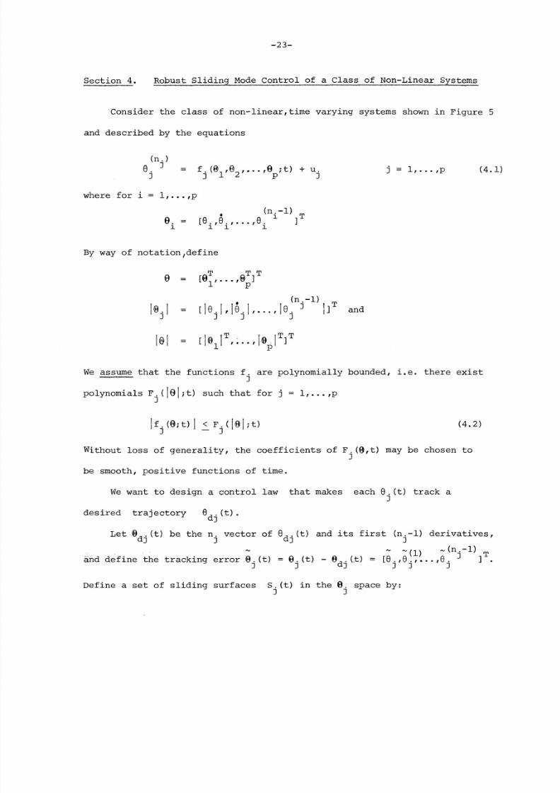
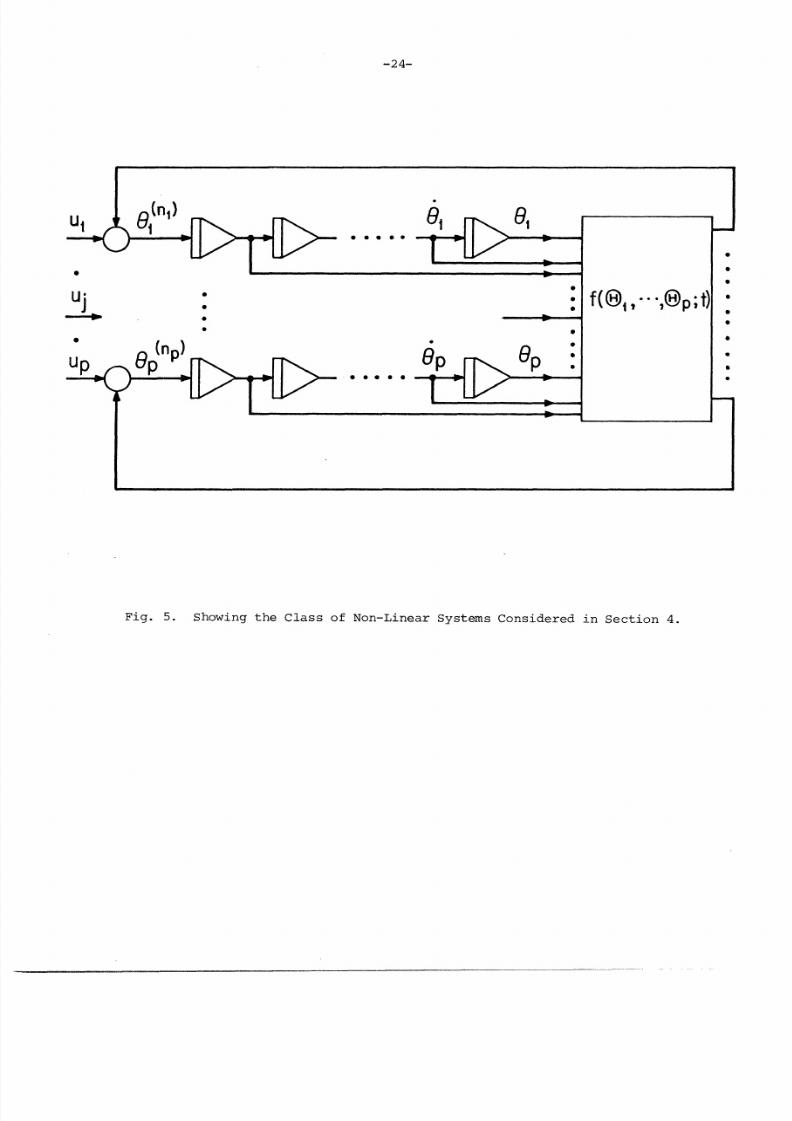
Section 4. Robust Sliding Mode Control of a Class of Non-Linear Systems

Consider the class of non-linear,time varying systems shown in Figure 5

and described by the equations

(n.)

0.j f( 82 '.. 8p ;t) + u j = ...,p (4.1)j12 p J

where for i = 1,...,p

·(n.-l)

8. = [ie.,..e., 1]

By way of notationdefine

oT T T

1 p

(ni.-1)

b@jI = [0lj,...l0. and

1 = [loI ,.T IT]T/Q/ 1 p

We assume that the functions f. are polynomially bounded, i.e. there exist

polynomials Fj(J0| t) such that for j =

If. 1;t)J < F.(I9I;t) 4.2)

Without loss of generality, the coefficients of F.(0,t) may be chosen to

be smooth, positive functions of time.

We want to design a control law that makes each .(t) track a

desired trajectory dj (t).

Let (dj(t)e the n. vector of edj(t) and its first (n.-l) derivatives,

(1) (n.-l) T

and define the tracking error 8j(t) = 8j(t) - dj (t) = [0j,j,...,0

Define a set of sliding surfaces S.(t) in the 8j space by:7 7



-24-

U..~~~~~~~~~~~~~~~~0, p;t)

Fig. 5. Showing the Class of Non-Linear Systems Considered in Section 4.

J ~ ~~~~~~~~~~ ~ -------- ~~----~



-25-

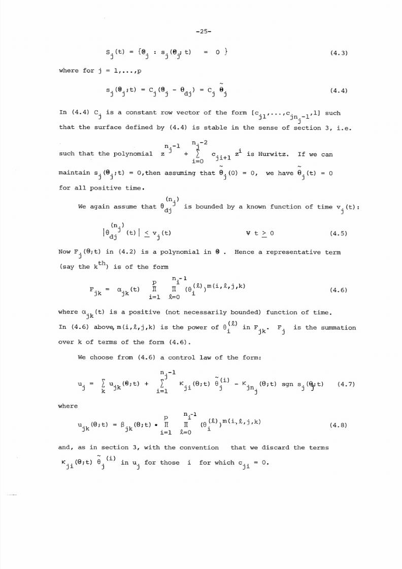
S.(t) = { :. 0j; t) = 0 } (4.3)3 3 33

where for j = l,...,p

sj(Oj;t) = Cj(j - 0dj) = C.j . (4.4)

3 j j dj j3 3

In (4.4) C. is a constant row vector of the form [c . .,c 1,l] such

that the surface defined by (4.4) is stable in the sense of section 3, i.e.

n.-2

such that the polynomial z 3 + cjC l zi

is Hurwitz. If we can

i=0

maintain sj (.;t) = 0,then assuming that 0.(0) = 0, we have 0.(t) = 0

for all positive time.

(n.)

We again assume that edj is bounded by a known function of time v.(t):

(n.)

l d (t)I < vj(t) v t > 0 (4.5)

Now F.(8;t) in (4.2) is a polynomial in 0 . Hence a representative term3

(say the k ) is of the form

n.-lp 1

F9(t) I (e(z))m(i

'

z,j,k) (46)Fjk = ljk i-l i (4.6)

where ajk t) is a positive (not necessarily bounded) function of time.

In (4.6) above,m(i,i,j,k) is the power of i) in Fjk. F is the summationjk i

over k of terms of the form (4.6).

We choose from (4.6) a control law of the form:

n.-l

u =k uk ;t) + Kji (0;t) e. - Kj (0;t) sgn sj (0;t) (4.7)k jk jii=l ]n.

where

n.-1p 1

ujk(0;t) = jk(8;t) * iT I '(ik (4.8)

i=l ==o

and, as in section 3, with the convention that we discard the terms

K. 8;t)08 i) in u. for those i for which c.. = 0.31 3 3 31





-27-

The approach though complicated notationally is simple in spirit, as

the example below shows. Though the control problem is a multi-input

problem,it is in effect treated as p single-input problems: the j sliding

surface s.j(.;t) depends only on 0j (it involves no contraints on the 0kJ J J

for k 7 j)- Also, in the choice of u. the terms in 0k for k f j are treated3 k

as disturbances as the example shown below explicates.

Example

Consider the system described by the equations

.. 2 0

1 = 36 + 62 + 2.16e2 cos 2 + u (4.14)

to 3

62 =1 - cos 81 · 82 + U (4.15)

The problem to be addressed is to get 81, 62 to track the parabolas

2t2

and t2

respectively. The sliding surfaces S and S are chosen with1 2

this objective in mind as

sl(01 t) = 1 + 01 - 2t(t+2) = (4.16)

and s2(2',t) = 62 + 02 - t(t+2) = 0 (4.17)

Note that (4.16) and (4.17) are the differential equations governing the two

parabolas. Consider first the choice of ul of the form (4.7),namely:

Ul l11 1+ 12 2+

13 a1 2 + 111 4t) - K12 sgn s

then, we have

1 d 2 2

2 dt S1 = 1 1 11 3) + s 2( + 1) + s182(13 2 cos 82)

+ S1(61 - 4t) (K 1 1 + 1) - K1 2 I 1 - 4 S1



-28-

In accordance with the prescription suggested above,we choose the jk as

follows:

Sl 0 l > 0 B1 -3 sl < -3

1 > O 0 < - 1 < 0 _ 2 > -1

12 > 13< -2 s 2 < 0 13 +2

sl'(l- 4t) > >K11 < -1 s1 61l- 4t) < 0 K 11 > -1

and K > 412

For the choice of u 2, consider again the form

= 3 +K (2 -2t) - K22 sgn s2 = 21 1 222 + 212 2 2 sgns 2

Then, we have

id 2 3dt 2 1 s2 21 + 1) + S282(22 cos 81) + s2(02 2t)(K21 + 1

2 dt 2 1 2 21 22 22 1 2 2 21

K2 2 1S21 - 2s 2

The jk are now chosen as follows:jk

s201 > 0 -B21 -1 s201 < 0 = 21 > -1

sO2 > 0o 22~-1 s <-< o-, >_ 1

s2(e-2t) > 01 < -1 s2.(-2t) < 0 >K21 > -12 Bz21 - s2K 21-

and K2 2 >2

By a minor modification of the foregoing procedure,it may be extended

to the control of systems of the form

(n.)

0. i = 1 ;t) + b.(p;t) t).J J p j J



-29-

so long as the b (8,t) are of constant sign, say positive, and bounded

as follows

<Xj.(t)

<b.j(;t)

< j (t)

The right hand sides of equation (4.9) - (4.12) are then replaced by

3jk(O;t) = >j3t)jk(t)/Xj(t)

Bjk(O;t) j=(t) > ajk(t)/Xj(t)

and

Kji((;t) = K i t) > Max(-cji/j (t), - cji/j(t))31 31 j i3)i

K t) = K+ (t) < Min(-c..ji/X.. (t), - c (t)ji ji 31 3 31

respectively.

As in Section 3, the effect of time variation of parameters in the

right hand side of (4.1) and of disturbances d. (@;t) in each of the equations

(4.1) can be nullified by suitable choice of u.j(O;t). Consider,for instance,

insensitivity to disturbances. Let the disturbances d. ;t) in the right

hand side of (4.1) satisfy

n -1

p 18kl )

Im (i' l' j' k )

(4.18)Id.j(8;t)I < .(t) + jk(t) II I )mi4183 - Do k jk i=l = (4.18)

with the jk(t) positive functions of time. The sliding condition (2.12)

is then satisfied if the right hand sidesof equations (4.9), (4.10), (4.13) are

modified as follows:

jk (t) >ajk(t) + .jk t) (4.19)

jk(t) jk(t) () (4.20)

K. (O;t) > v.(t) + 6. (t) uniformly in t (4.21)Jn. 30

3



-30-

respectively. Equations (4.11), (4.12) are not modified.

Of course,if there are terms of the form (> ))m(i, j,k) included in

(4.18) which are not present in (4.6), then corresponding terms in ujk need

to be included in order to satisfy (4.19), (4.20).

Consider the application of this procedure to the system of the example f

with equation (4.14) replaced by

2

1 = 381 + + 281 82 Cos2 + u + d 1 (0) (4.22)

with dl satisfying

Id1 1) I < 610+ 111 (4.23)

The terms 311 and 12in the control law need to be modified in accordance

with (4.19) - (4.21) to

s ' 81> 0° 11 < -3 - 611 s 1- 81 < 0° 7.^11 > -3 + 611

and K12 > 4 + 610

in order to retain the tracking in the presence of the disturbance d1.

Note, as before, that the magnitude of the discontinuity in the control

law is proportional to the magnitude of the disturbance. Also, once the

trajectory is on a sliding surface S. (t),its dynamics are governed by

n.-2- (n.-1) 3ej + E CJl e(i) (4.24)

3 ~i=0 ji+l j

which does not contain the disturbance term.

The choice of C. such that the surface defined in (4.24) is stable proves

particularly useful in Section 5, where we replace the idealized discontinuous

control law of this section by a continuous control law which approximates u

in a suitable sense.



-31-

We remark here that the development of this section using the poly-

nomial bounds of equations (4.2), (4.18) can be generalized when fj(O;t),

dj(e;t) are bounded by other classes of functions. For instance, if the

disturbance dl in (4.22) is a function of 01 and 02 and satisfies (instead

of (4.23))

Id, ) < 610 + 61111el + exp 8 2

then we modify the control law u1 to contain in addition a term of the

form ~14 exp 82 where

s1> 0=- 614 < -1 and s1 < 0 14 > 1



-32-

Section 5. Continuous Control Laws to Approximate Sliding Mode Control

The usage of discontinuous or switched control to generate robust

control laws is not without a price. In practice, imperfections such

as delays in switching, hysteresis in switching, ill cause the trajectory

to chatter along the sliding surface as was illustrated in Section 2.

This will of course be accompanied by a rapidly (time)-varying control

law. Chattering is undesirable both in itself and in the fact that it

represents a 'high frequency' signal component in the state trajectory,

which may excite unmodelled 'high-frequency' dynamics. Thus, while

sliding mode control provides control laws which are robust to parameter

variations and disturbance inputs, they are, in themselves, not robust to

the usual modelling approximations (i e., neglect of dynamics which lie

outside the frequency range of interest) that go into control system design.

We seek in this section to remedy this situation by replacing the dis-

continuous or switched feedback laws of the previous section by continuous

control laws which will preserve the disturbance rejection properties of

sliding mode control, and in addition not generate undesirable high

frequency signals.

The basic idea is simple: it consists of 'smoothing' out the dis-

continuity in the control law at the switching surface, i.e., find,

in the notation of Section 4, a continuous control law u.(0;t) whose

terms are continuous functions of ~ inside.a small boundary

layer neighboring the switching surface . The boundary layer then

plays the role of a smudged switching surface i.e., trajectories starting

outside the boundary layer converge to it and further, the positive



-33-

invariance of the boundary layer is robust to parametric variations in

the dynamics outside. The penalty paid for smudging the sliding surface

is that the dynamics of the state trajectory inside the boundary layer

are only an approximation to the desired dynamics on the sliding surface.

The advantage of the scheme is that the state trajectory does not

chatter very rapidly close to the sliding surface - in fact the wider the

boundary layer, the lower the chatter, but the lower the tracking accuracy.

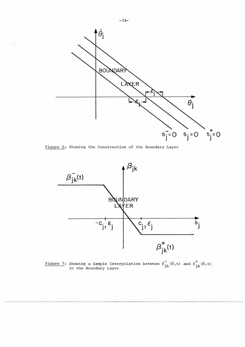
To carry out the preceding program we use again the class of stable

sliding surfaces considered in section 4/ with the sj(j;t) of the

form:

s. B.;t) = C.R. (t) (5.1)

To define the boundary layer about the sliding surface of (5.1), define

s(j.;t) = sj(j.;t) + c. sj (5.2)

and

s+(0j;t) = s.j(j;t) - Cj.j (5.3;)J J J J J1 J

Figure 6 shows the relative position of the surfaces s.=O, s. =0 and

s. = 0 for the case that n. =2. Note that c >0 since 4.2) is Hurwitz.

The boundary layer B. (t) is defined by

B.(t) = { : . (.;t) > 0 and s. .;t) < 0} (5 4)

It is immediate from (5.2) and (5.3) that

d - d d +

dsj j;t) dt sj (;t) . (.;t)t~~~~~~~~3jt 33 d





-35-

We choose control law u.j(;t) as given by (4.7)-(4.13) for

e {@ s. .;t) < 0} or 0 e {9:s.(9.;t) > l0} .e. outside B.(t). This

guarantees that

d sT(®.;t) > 0 for 8 e {9:sj 1.;t) 0} =:S (t) (5.5)dt j j -

and

d + + +dt s+(O.;t) < 0 for 8 e {e:s. (O.;t) > 0 =:S(t (5.6)dt j 3 ] 3 3

(5.5) and (5.6) establish (by the same arguments as in Section 2) that

trajectories starting outside B.(t) tend towards B.(t), and further

trajectories starting inside B. (t), stay in it for all future

time. It only remains to specify u.j(;t) to be a continuous function of3

8 inside B.(t). We claim that any continuous interpolation between3

u.j(;t) defined on Sj(t) and u.j(;t) defined on S (t) will suffice

for our purposes (at least one such interpolation exists, by Urysohn's

lemma [41). Figure 7 illustrates a sample interpolation for one of the

p i

ajk(9;t) of (4.9) , (4.10) in the case that In (8(Q))m(i ,ik) > 0

... t ........ i=l

at time t±. Similar interpolations are to be performed for the Kji(O;t).

We now show that with the preceding choice of the control law

u. (9;t), 0 (t) tracks dj(t) to within a small error linearly proportional

to E. (in articular, the error goes to zero when e. does). Note that

3 3

with the preceding choice of continuous control law the trajectory

0(t) satisfies a regular differential equation. Further, if at t=O,

(0) e B(0) then P(t) e B(t) for all time. Hence

t~ p n l

For the case I i (. ) )m (i 'j k) <O eplace sj by -sj in Fig.7.

i=l =01



-36-

sj (j;t) = cjlA(t) V t>O (5.7)

where A(t) is some function satisfying

JA(t)J < j

Using the form of s.j(j;t) given by (5.1) it is then possible to bound] 3

0~jt) - jd(t) , using elementary linear algebra. It is easy to

verify for instance, that if s.j(j;t) is chosen to be of the form

d n.-l

sj(8j t = (dt+ j d

then with j(0) = dj (0) the tracking accuracy is

|1. t) - 6 . t)| < E. V t>O. (5.8)3 d3 - 3

In the instance that j. 0) does not exactly match dj(0), (5.8) is modified3 dj

to

6j8(t)- 6 (t) < . + P(t)(t)+ P(t) O)exp-t Vt > 0

with P(t) a polynomial in t.

An examination of (4.9)-(4.13) shows that the control law u (0;t)

of equation (4.7) is discontinuous not only acrossthe surfaces {f:s.=0},but also

across the surfaces given by {e: ) =0} for those i,Z for which some m(i,Q,,j,k)

in (4.6) is odd,and across {O:O. =0}. However, as noted in section 4,3

surfaces of the last two categories are not sliding surfaces (in particular

our solution concept calls for a unique extension of trajectories

through them). Hence, we need not replace the discontinuous control law

at these surfaces by a continuous one - and, of course, no high frequency

chattering is generated at these surfaces by switching imperfections.



-37-

We now illustrate the application of the methodology of Sections

4 and 5 to the control of a two-link manipulator.



-38-

Section 6. Application: Sliding Mode Control of a Two-Link Manipulator

The accurate,high-speed tracking of desired trajectories is the

control-challenge in the development of modern industrial robots and

manipulators. Typically, the equations of motion of these robots are

highly non-linear and coupled. Also, the development of flexible manu-

facturing systems calls for robustness of performance with regard to

the variation of the load, task or real time trajectory specification,

as well as other 'disturbances . Given these complexities, no viable

control methodology has asyet been proposed for these problems.

In general, the dynamics of industrial robots can be described

by equations of the form (4.1), with bounds of the form (4.2) arising

from the presence of sine and cosine terms (as shown in the sequel).

System parameters undergo variations because of variations in the loads

in a flexible manufacturing system environment, variations in the ambients,

imprecise modelling and the like. We describe the application of 'our

procedure to the robust, sliding mode control of a two-link manipulator.

In Section 4, we showed how a multiple (p) input -control problem was

decomposed into a set of decoupled single-input problems. By

this token, we see that the complexity of our design procedure for a

more sophisticated manipulator involving more than two links is not

significantly increased. By design, our sliding mode feedback controller

is robust to certain variations in parameter values, an improvement over

the 'non-linear decoupling techniques' roposed by Freund [3]1, on-line

computational schemes proposed by Luh, et al [6], [13], and the linearization

techniques of Melouah, et al. [14].



-39-

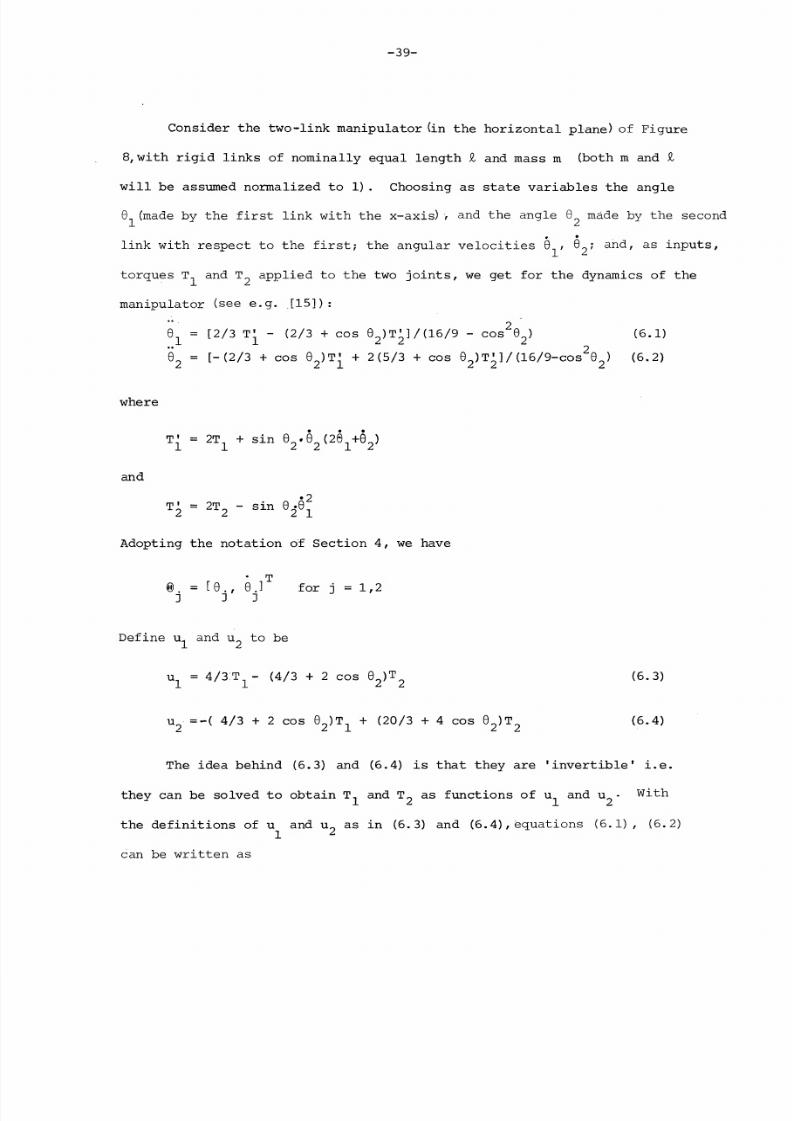
Consider the two-link manipulator (in the horizontal plane) of Figure

8, ith rigid links of nominally equal length Z and mass m (both m and k

will be assumed normalized to 1). Choosing as state variables the angle

l(made by the first link with the x-axis)-, and the angle 82 made by the second

link with respect to the first; the angular velocities 01' 02; and, as inputs,

torques T 1 and T 2 applied to the two joints, we get for the dynamics of the

manipulator (see e.g. [15]):

2

81 = [2/3 T - (2/3 + cos 02)T']/(16/9 - cos 82) (6.1)

O2 = [-(2/3 + cos 02)Ti + 2(5/3 + cos 82)T']/(16/9-cos80 62)

where

TI = 2T + sin 820.2(21+0 2

and

T 2 = 2T - sin 08.0

Adopting the notation of Section 4, we have

* T0. = [j., e.] for j = 1,2

Define u1 and u2 to be

u1 = 4/31T 1 - (4/3 + 2 cos 82)T2 (6.3)

u 2 =-( 4/3 + 2 cos 02)T 1 + (20/3 + 4 cos 02)T2 (6.4)

The idea behind (6.3) and (6.4) is that they are 'invertible' i.e.

they can be solved to obtain T 1 and T 2 as functions of u 1 and u 2- With

the definitions of u and u 2 as in (6.3) and (6.4),equations (6.1), (6.2)

can be written as



-40-

y

T2Figure: ATwo-Linkanipulator

Figure 8: A Two-Link Manipulator



-41-

81 = [2/3.sin 2e (261 + 2) - (2/3 + cos in 6 + ul]/(16/9 cos2 2)

~/11 2 1 2

(6.5)

02 = [-(2/3 + cos 82)sin 82e6(261+62 ) - 2(5/3 + cos 82 )sin 2 1+u ](16/9 -cos

(6.6)

The aim of the design is to get .(t) to track a desired trajectory3

dj (t) (for j=1,2). Accordingly, we choose

s. (j ;t) = -dj) + 5(0j-6dj) for j=1,2 (6.7)

and we assume as in (4.5) that 6dj is bounded, specifically that:

2dj t)WI < 1.75 rad./sec. (6.8)

(6.8') is the only a priori information required regarding8dj

As in Section 4, we choose ul and u2 to be of the form

U. 26 ) * +K * sns(6.9)l 112 1+2 + 12 1 1 1- dl 12 sgn 6.9)

2 = 212 26 +62) + 21(62-0d2d K22 sgn s2 (6.10)

We choose to keep the terms6 2 (261+62) grouped in (6.9), (6.10),

since they appear in this form in the system description (6.1), (6.2).

The surface {@:261+6 2 = 0} is not a sliding surface in the following

development since trajectories can be uniquely continued through it.

Again, proceeding as in Section 4, we chose for the control law:

= 3-+ = 1.27

12 21 12 21



-42-

-jl -3 ·4.422 22

38 K = ; Kj2 = 3.15 for j=1,2ji jl j2

The preceding manipulations yield a discontinuous control law.

Following the development of Section 5, we obtain a continuous control

law inside B.(t) given by3

K Js./5s Ij2 j j

in place of Kj2 sgn sj, and similar linear interpolations for the

jk and Kjl. Both E 1 and C2 are chosen to be 10.

Given the values of u1 and u2 in (6.3) and (6.4), we solve for

T 1 and T2 ' the real control inputs for the manipulator.

A digital simulation of the preceding control scheme was performed

using a sampling rate of 50 Hz. The simulation also added random measurement

noise (uniformly distributed on the intervals [0, 0.25] degrees for angles,

and [0,0.5] degrees per second for the angular velocities) to study

experimentally the robustness of our proposed scheme to noise, a topic

that remains to be studied analytically. The motion of the manipulator

was simulated with the aid of a fourth order Adams-Bashforth, algorithm

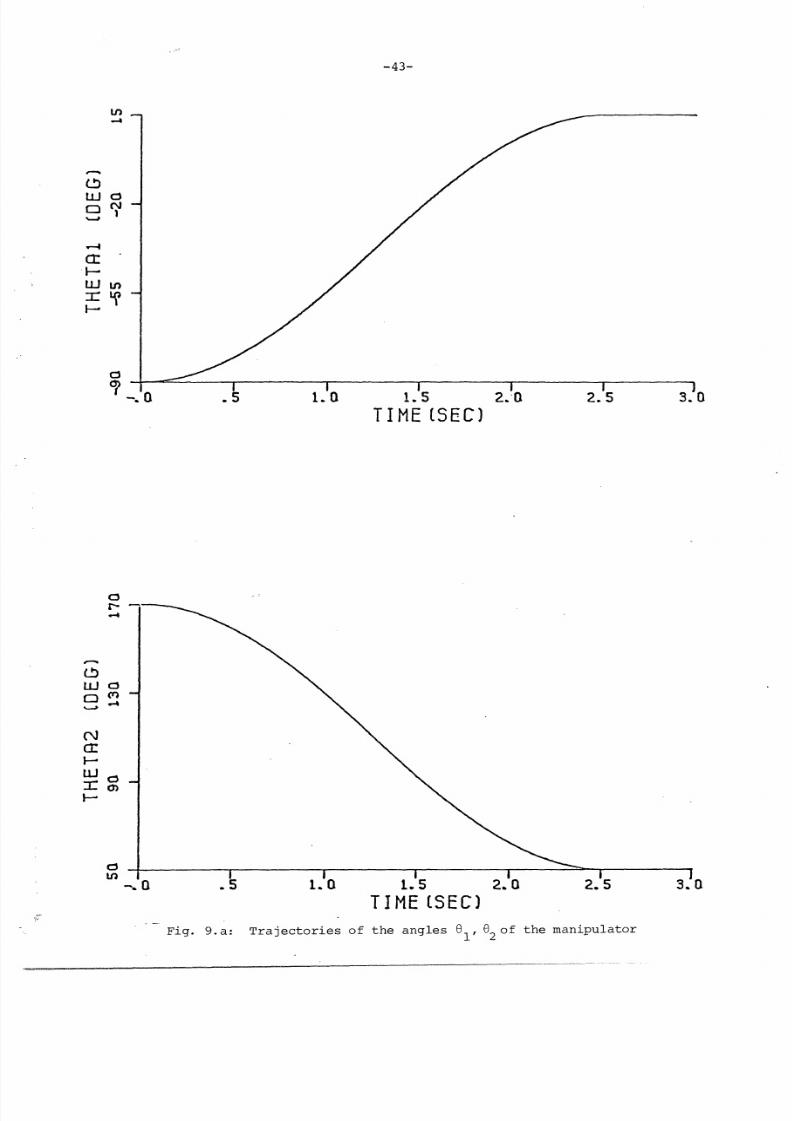
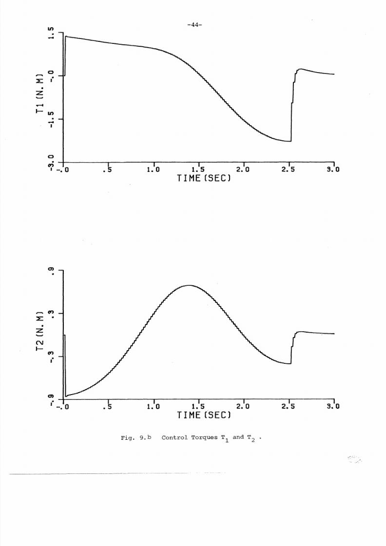
(with fixed step size of 6.67 milliseconds). Plots of the simulated

trajectory of the manipulator are presented in Figure 9 (the rate of the

plotter was 150 points per second). The manipulator was initially idle

at 01 = -90°, 62 = 170

°and was required to track

1 '2



-43-

bo

lJ m~~Jt -4

-Q ,,5 1.0 1.5S 2:10 2.15 3. 0

TIME (SEC)

0

eLJ O

CnCto

U, - \v . \

_,0 .5 1.0 1 5 2.0o 2 5 3.0

TIME SEC)

Fig. 9.a: Trajectories of the angles 1, 02 of the manipulator



-44-

o. l

I

I

C3

J- .5 1. 1.15 2.0 2.5 3.0

TIME SEC)

CD

( n

Cr,)

,* I I I5 2 2-.0 .5 1.0 1.5 2.0 2.5 3.0

TIME SEC)

Fig. 9.b Control Torques T1 and T2



-45-

dl (t) =-90°+ 52.50 (1-cos 1.26 t) for t < 2.5

150 for t > 2.5

d2 (t) = 1700 - 600 (1-cos 1.26 t) for t < 2.5

= 50°

for t > 2.5

which satisfy equation (6.8) with the angles dl(t), d2(t) measured in

radians. The computational delay is one sampling time.

The simulation results show tracking to within an error of .70 in

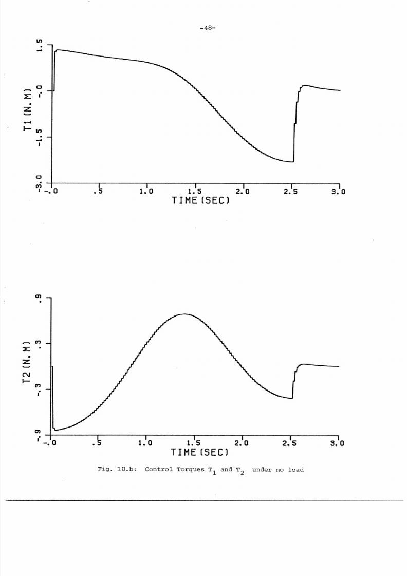
81 and 82. Note that edl6' 2 and hence T1, T2 are discontinuous at t=2.5.

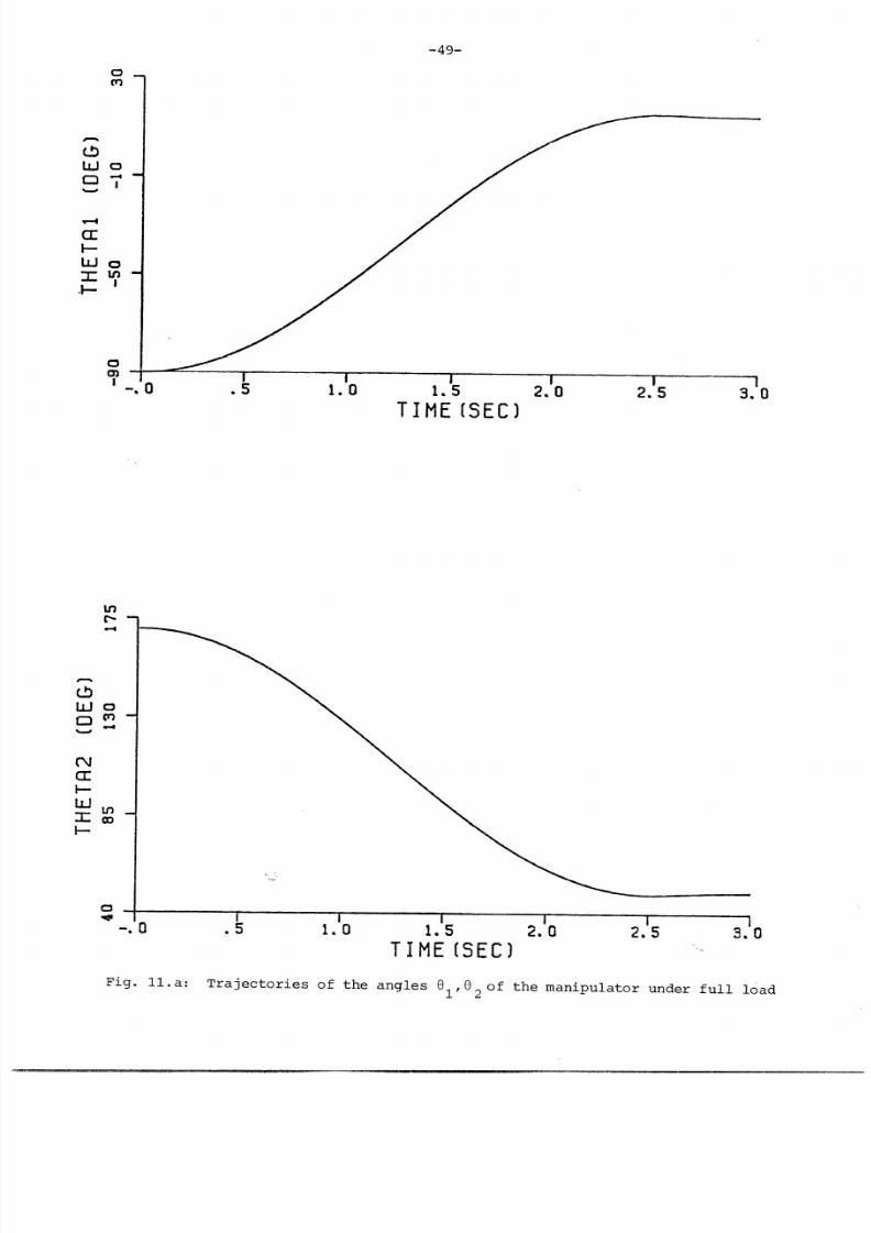
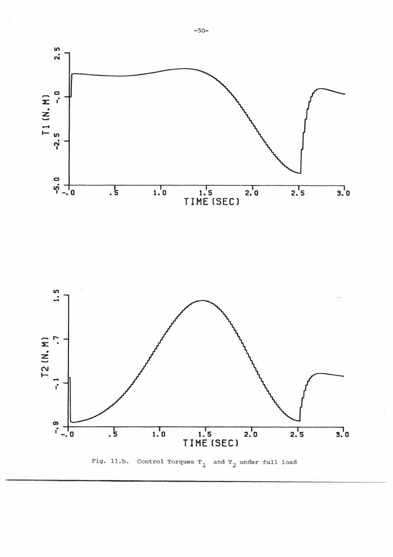
To show the robustness of our scheme to parameter variation,we

demonstrate how a modification of our control law results in tracking in

the face of varying load 1r (between 0 and 0.25) at the tip of the

load arm. The system equations are then modified to (see e.g. [15]):

61[2(5/3+cos 82) + 4p(l+cos 82)] + 82[2/3 + cos 82 + 21(l+cos 62)]

2T1 + sin 82 62 ' (2 1+62)(1+2p) (6.11)

-282[2/3 + cos 82 + 2p(1+cos 2)] + 82[2/3 + 21] = 2T2 - sin 80 1(1+2p)

(6.12)

To keep (6.7) a sliding surface fori belonging to [0,0.25], we choose

the control law of (6.9) and (6.10) with

- +f =-f3 1.211 11

+ +3 =3 =43 =-f3 =2.112 21 12 21

3 =43 =6.422 22

Kjl = -2.4 ; Kl = -15.2 for j=1,2jl j



-46-

The modification of the terms K12 and K22 in the control law is more

involved. The disturbance term in ul, u2 of (6.3), (6.4) caused by the

presence of i in (6.11), (6.12) includes terms in T 1 and T2. This leads

us to choose the kj2 to contain terms in T 1 and T2:

K1 2

=5.5 + IT2 1/2 6.13)

K22 = 5.5 + IT1 1/2 + IT21 6.14)

From an inspection of the values of T 1 and T2 in simulations, we

found that their variation was small and that (6.13), (6.14) could be replaced

by constant K1 2, K 2 2 using conservative bounds on IT1 1 and ITT2.

Plots of the simulated trajectory of the manipulator with this modified

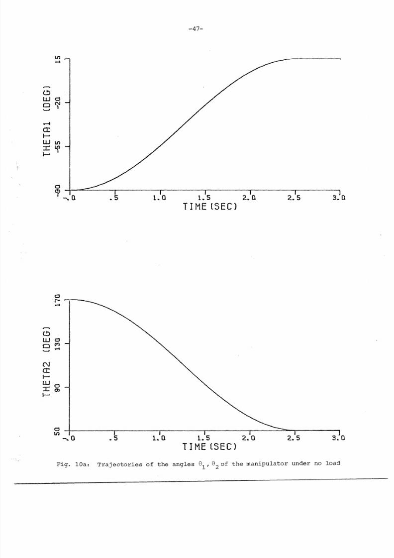
control law, tracking the same Odj as before,are presented in Figure 10

(for the no-load, P=0.case) and Figure 11 (for the full load, 1=0.25 case).

The idealized control laws are approximated by continuous control laws

exactly as before and yield tracking precision of 0.9°

for the no-load

case and 1=9°

for the full-load case, with El = E2 = 2.5 . The tracking

error may be decreased by decreasing the sampling time and the £ s.

Young [11] has proposed the use of classical sliding surface

methodology to stabilize a two dimensional manipulator,and has suggested

extensions to tracking. Our approach is explicitly for the purpose of

tracking and does not involve a 'reaching' phase to the sliding surface.

By decoupling a multiple-input problem into several single-input problems,

we avoid the problems associated with reaching a 'hierarchy' of sliding

surfaces. By smudging the control across the discontinuity surface we

mitigate the extent of the chattering.



-47-

vL n

Ct:F-

-~

.5 1.0 1.5 2. 2.5 3.0

TIME1SEC

FT cat

LU 0

_,a0S 15 1.5 2.0 2.5 3.0

TIME (SEC)

Fig. 10a: Trajectories of the angles 61, 02of the manipulator under no load





-49-

- 1

-.0O .5 1.0 1.5 2 0 2 5 3.0

TIME SEC)

in

-

dJ\

N

32\o

-. .5 1. 0 1.5 2.0 2.5 3.0TIME SEC)

Fig. ll.a: Trajectories of the angles 6, 02 of the manipulator under full load

· ~~ ~ ~ ~ ~ ~ ~ ~ ~ ~ ~ 1 2--~~--~- p--·---I··-··--*···-- _I- --··O



-50-

In

0 .5 1. 0 2. 0 2. 5 3. 0

TIME SEC)

0,

- ---0 .5 1.0 1.5 2.0 2.5 3.0TIME SEC)

Fig. ll.b. Control Torques T 1 and T 2 under full load

.n ~ ~ ~~~~~ ~~~~~ 2~



co

'½-a

WII 1Cv

-90 -50 -10 30

THETAR1 DEG)

co

4o

440 85 130 175

THETR2 DOEG)

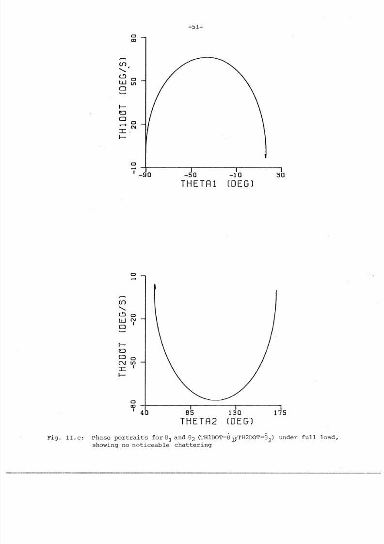
Fig. ll.c: Phase portraits fore, and 02 (TH1DOT=Ul;TH2DOT=e2) under full load,

showing no noticeable chattering



-52-

Section 7. Areas of Further Research

Certainly the present paper is only a step in developing the

sliding-mode control methodology for the robust control of a class of non-

linear time-varying systems. The methodology needs to be extended to more

general classes of non-linear systems than those discussed in Section 4.

In its present form,the feedback control law uses full state feedback -

the case of output feedback (with observers) remains to be investigated.

In a related context, the effects of measurement noise and process noise

on the sliding mode control methodology have yet to be studied. The

continuous control laws of Section 5 were derived in order to trade off

the generation of undesirable high frequency signal against tracking

accuracy. The precise nature of this trade-off needs to be quantified.

Finally, the use of sampled-data control to implement the sliding mode

control presents new problems in the analysis of the resultant hybrid

scheme. While sampled-data control was in fact used successfully in the

example of Section 6, we believe that further research needs to be

done in this direction of implementation.

Finally, we have used the currently important area of manipulator

control as the trial area for our methodology. We are now in the process

of implementing sliding mode control laws on different kinds of manipulators

and simulating their performance. Given the inherent non-linearities

involved in all but Cartesian manipulators, we feel that our methodology

is particularly suited for this application.



-53-

ACKNOWLEDGMENTS

The authors would like to thank Prof. W.E. VanderVelde for invaluable

comments and suggestions.

This work has also benefited greatly from stimulating discussions with

Dr. P.K. Chapman, Prof. T.L. Johnson, Prof. P.V. Kokotovic, Prof. M.

Pelegrin, and Prof. W.S. Widnall.





-55-

[15] Horn, B.K.P., K. Hirokawa, V.V. Vazirani, Dynamics of a Three Degree

of Freedom Kinematic Chain , M.I.T., Artificial Intelligence Laboratory,

Memo 478, Oct. 1977.

Documents

J.J. Slotine and S.S. Sastry 11