Embed Size (px)
Citation preview
Júlia Dégi
DETAILED STUDY OF MAFIC LOWER CRUSTAL XENOLITHS FROM
THE BAKONY–BALATON HIGHLAND VOLCANIC FIELD
RELATIONSHIPS BETWEEN METAMORPHIC PROCESSES IN THE LOWER CRUST
AND THE FORMATION OF THE PANNONIAN BASIN
PhD Thesis
Ph.D. program for Geology and Geophysics at the Ph.D. school of Earth Sciences
Eötvös Loránd University, Budapest
Chair of the Ph.D. school and leader of the Ph.D. program for Geology and Geophysics:
Prof. Dr. Miklós Monostori, D.Sc. Dept. of Paleontology, Eötvös University
Supervisors:
Dr. Kálmán Török, Ph.D.
senior researcher , Eötvös Loránd
Geophysical Institute of Hungary
Dr. Csaba Szabó, Ph.D.
associate professor, Dept. of Petrology and
Geochemistry, Eötvös University
Consulent:
Prof. Dr. Rainer Abart, Ph.D.
full professor, University of Vienna
Lithosphere Fluid Research Lab
Department of Petrology and Geochemistry Institute of Geography and Earth Sciences
Eötvös University, Budapest
Department of Mineralogy, Petrology, Geochemistry
Institute of Earth Sciences Free University Berlin
Eötvös University, Budapest, Hungary, 2009
„Before proceeding, however, it must be made clear that we, like our critics, accept without qualification the ground rules imposed by classical thermodynamics and its subsequent application to heterogeneous equilibria as developed by Gibbs (1928). We thus adhere to the same gospel, if not the same interpretation of it.”
J.B. Thompson (1970)
ACKNOWLEDGEMENTS
First of all, I am grateful to my family, especially my husband. This thesis would not exist
without their patience, love and support in the five years of my PhD work.
I would like to thank everything for my mentors Dr. Kálmán Török, Dr. Csaba Szabó and Dr.
Rainer Abart. My supervisors, Dr. Kálmán Török and Dr. Csaba Szabó have drawn my attention to
xenolith research and they have been supporting me from the very beginnig. They taught me the
basics of metamorphic petrography and fluid inclusion research, and they helped me whenever I
needed with fruitful discussions and wise advices. My consulent, Dr. Rainer Abart had a key role in
my stay in Berlin. He helped me a lot in preparing the proposals for scholarships and scientific
collaborations and he guided me into the world of micro- and nanoscale processes and high
resolution analitycal techniques.
The dataset giving the basis of this PhD thesis is very large and many people from many
laboartories contributed to it. I acknowledge the help of Margit Csömöri, Frau Behr and Frau Anja
Schreiber in sample preparation; of Dr. Kálmán Török and Dr. Kamilla Gálné Sólymos in
micropobe work in the Eötvös Univeristy, of Dr. Harvey E. Belkin in micropobe work in the United
States Geological Survey, Reston Headquarters; of Dr. Ralf Milke in micropobe work in the Free
University Berlin; of Dr. Dieter Rhede in the work with the FEG-EPMA; and of Dr. Richard Wirth
in FIB-TEM work both in the GFZ German Research Centre for Geosciences, Helmholtz Centre
Potsdam. I would like to thank Dr. Lutz Hecht providing microprobe standards for Fe–Ti oxides. I
am grateful to the data provided by János Kodolányi and Eszter Badenszki which were produced in
the University of Vienna with the help of Dr. Theodoros Ntaflos and Dr. Friedrich Koller. Dr.
Kálmán Török also provided his data measured in the Eötvös Univeristy.
Being a member of the Lithosphere Fluid Research Group has always been a great pleasure to
me. I am grateful to all members who were friends and collegues at the same time. Special thanks
to János Kodolányi and Eszter Badenszki who were working on mafic granulites as well and who
collected significant part of the dataset included in the thesis. Thanks for Enikő Bali, who provided
data and who had a key role in developing and constructing the Deep Lithosphere Database
(DLDB). I would like to thank to Károly Hidas and Zoltán Koncz for testing and debugging the
DLDB. Klára Kóthay helped a lot in understanding the xenolith – host basalt interaction by
providing mineral chemical data from the host basalt. I am garteful to Márta Berkesi who helped a
lot in making the GRANULITE database more understandable and user-friendly. I highly
appreciated the fruitful discussions with István Kovács, György Falus, Zoltán Zajacz, and all other
members of the Lithosphere Research Group.
I am proud to be involved in the FOR741 DFG research group for nanoscale processes in
geomaterials. I would like to thank all members of this research group for providing perfect
athmosphere for intense research in Berlin and Potsdam. I profited a lot from the group seminars. I
highly appreciated the discussions with Dr. Elena Petrishcheva, Dr. Ralf Milke and Dr. Wilhelm
Heinrich.
My collegues in the Metals Research Department, Research Institute of Solid State Physics and
Optics of the Hunagrian Academy of Sciences assisted me in the last year of my PhD work. I would
like to say thanks for their patience, understanding and encouraging during this critical period.
I acknowlegde the financial support of the following organizations, institutions, scholarships and
grants: PhD scholarship of the Republic of Hungary, the Lithosphere Fluid Research Group,
Hungarian National Scientific Foundation (OTKA K 61182), MTA-DFG scientific collaboration
(DFG/184, AB 341/4-1), Eötvös Scolarship of the Republic of Hungary, research scholarship of the
DAAD (A/07/91759), FOR741 DFG research group for nanoscale processes in geomaterials and
the Research Institute of Solid State Physics and Optics of the Hunagrian Academy of Sciences.
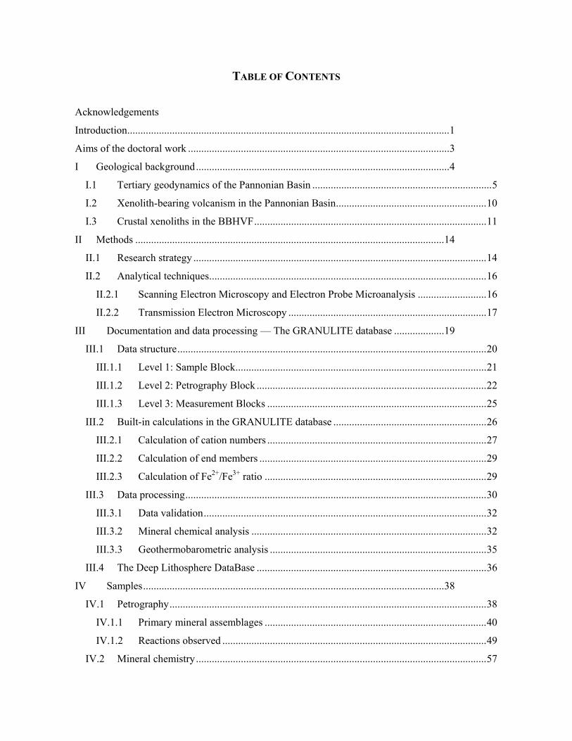
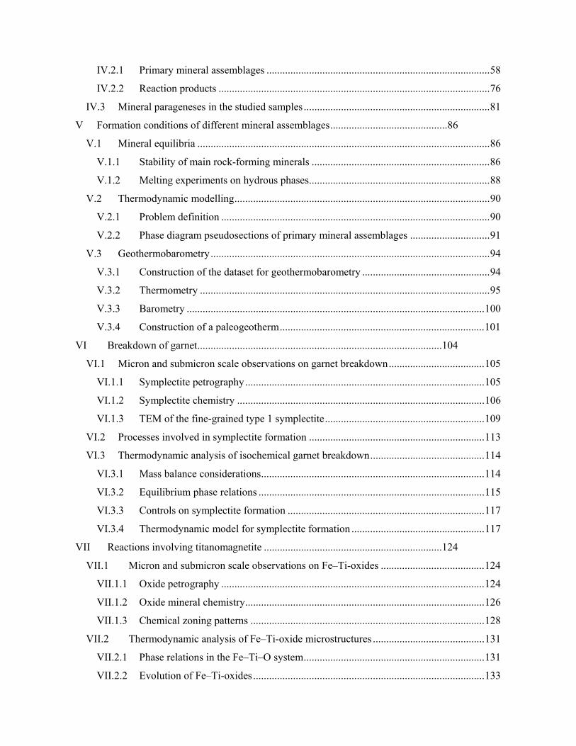
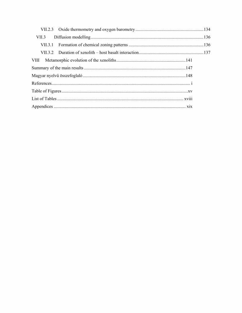
TABLE OF CONTENTS
Acknowledgements
Introduction..........................................................................................................................1
Aims of the doctoral work ...................................................................................................3
I Geological background................................................................................................4
I.1 Tertiary geodynamics of the Pannonian Basin ....................................................................5
I.2 Xenolith-bearing volcanism in the Pannonian Basin.........................................................10
I.3 Crustal xenoliths in the BBHVF........................................................................................11
II Methods .....................................................................................................................14
II.1 Research strategy ...............................................................................................................14
II.2 Analytical techniques.........................................................................................................16
II.2.1 Scanning Electron Microscopy and Electron Probe Microanalysis ..........................16
II.2.2 Transmission Electron Microscopy ...........................................................................17
III Documentation and data processing — The GRANULITE database ...................19
III.1 Data structure.....................................................................................................................20
III.1.1 Level 1: Sample Block...............................................................................................21
III.1.2 Level 2: Petrography Block .......................................................................................22
III.1.3 Level 3: Measurement Blocks ...................................................................................25
III.2 Built-in calculations in the GRANULITE database ..........................................................26
III.2.1 Calculation of cation numbers ...................................................................................27
III.2.2 Calculation of end members ......................................................................................29
III.2.3 Calculation of Fe2+/Fe3+ ratio ....................................................................................29
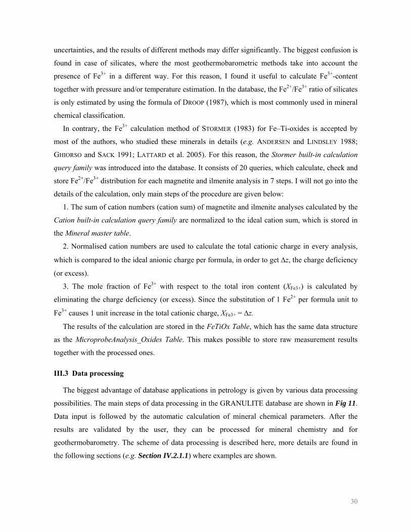
III.3 Data processing..................................................................................................................30
III.3.1 Data validation...........................................................................................................32
III.3.2 Mineral chemical analysis .........................................................................................32
III.3.3 Geothermobarometric analysis ..................................................................................35
III.4 The Deep Lithosphere DataBase .......................................................................................36
IV Samples..................................................................................................................38
IV.1 Petrography........................................................................................................................38
IV.1.1 Primary mineral assemblages ....................................................................................40
IV.1.2 Reactions observed ....................................................................................................49
IV.2 Mineral chemistry..............................................................................................................57
IV.2.1 Primary mineral assemblages ....................................................................................58
IV.2.2 Reaction products ......................................................................................................76
IV.3 Mineral parageneses in the studied samples ......................................................................81
V Formation conditions of different mineral assemblages............................................86
V.1 Mineral equilibria ..............................................................................................................86
V.1.1 Stability of main rock-forming minerals ...................................................................86
V.1.2 Melting experiments on hydrous phases....................................................................88
V.2 Thermodynamic modelling................................................................................................90
V.2.1 Problem definition .....................................................................................................90
V.2.2 Phase diagram pseudosections of primary mineral assemblages ..............................91
V.3 Geothermobarometry.........................................................................................................94
V.3.1 Construction of the dataset for geothermobarometry ................................................94
V.3.2 Thermometry .............................................................................................................95
V.3.3 Barometry ................................................................................................................100
V.3.4 Construction of a paleogeotherm.............................................................................101
VI Breakdown of garnet............................................................................................104
VI.1 Micron and submicron scale observations on garnet breakdown....................................105
VI.1.1 Symplectite petrography..........................................................................................105
VI.1.2 Symplectite chemistry .............................................................................................106
VI.1.3 TEM of the fine-grained type 1 symplectite............................................................109
VI.2 Processes involved in symplectite formation ..................................................................113
VI.3 Thermodynamic analysis of isochemical garnet breakdown...........................................114
VI.3.1 Mass balance considerations....................................................................................114
VI.3.2 Equilibrium phase relations .....................................................................................115
VI.3.3 Controls on symplectite formation ..........................................................................117
VI.3.4 Thermodynamic model for symplectite formation ..................................................117
VII Reactions involving titanomagnetite ...................................................................124
VII.1 Micron and submicron scale observations on Fe–Ti-oxides .......................................124
VII.1.1 Oxide petrography ...................................................................................................124
VII.1.2 Oxide mineral chemistry..........................................................................................126
VII.1.3 Chemical zoning patterns ........................................................................................128
VII.2 Thermodynamic analysis of Fe–Ti-oxide microstructures ..........................................131
VII.2.1 Phase relations in the Fe–Ti–O system....................................................................131
VII.2.2 Evolution of Fe–Ti-oxides .......................................................................................133
VII.2.3 Oxide thermometry and oxygen barometry .............................................................134
VII.3 Diffusion modelling.....................................................................................................136
VII.3.1 Formation of chemical zoning patterns ...................................................................136
VII.3.2 Duration of xenolith – host basalt interaction..........................................................137
VIII Metamorphic evolution of the xenoliths..............................................................141
Summary of the main results ...........................................................................................147
Magyar nyelvű összefoglaló ............................................................................................148
References............................................................................................................................ i
Table of Figures.................................................................................................................xv
List of Tables ................................................................................................................. xviii
Appendices ...................................................................................................................... xix
1
INTRODUCTION
The structure and evolution of the Mediterranean basins has been a current research topic for
several decades. Intense research interest on basin formation was initiated by the birth of the
thermomechanical basin evolution theory of MCKENZIE (1978). Since the Pannonian Basin system
was extremely well-studied, it was used as a model basin for the first application of the new theory.
Since then, this area continually serves as a source of information on lithosphere evolution in
extensional settings and as a model area of geodynamic models. Intense comprehensive
geophysical studies were done between 1980 and 1986 in order to apply the thermomechanical
basin evolution theory for the Pannonian Basin. The main results were summarized in the
monograph of ROYDEN and HORVÁTH (1988). It involved the investigation of surface tectonics of
the Pannonian Basin system and the surrounding orogens (ROYDEN 1988), biostratigraphical and
sedimentological studies (BÉRCZI 1988; BÉRCZI et al. 1988), the interpretation of reflection seismic
data (HORVÁTH and POGÁCSÁS 1988; RUMPLER and HORVÁTH 1988; TOMEK and THON 1988) and
map construction on the basis of temperature, thermal conductivity and heat flow data (DÖVÉNYI
and HORVÁTH 1988). Until now, several authors contributed to the refinement of the proposed
basin evolution model of ROYDEN (1988) by adding different types of information, such as
paleomagnetic data (BALLA 1987, 1988; MÁRTON et al. 1990, 2003), new field observations (e.g.
RATSCHBACHER et al. 1991a,b), new maps of crustal and lithospheric thickness variations (e.g.
POSGAY et al. 1991; HORVÁTH 1993), new palinspastic reconstructions (e.g. CSONTOS et al. 1992;
FODOR et al. 1999; CSONTOS and VÖRÖS 2004; KOVÁCS et al. 2007; KOVÁCS and SZABÓ 2008),
careful analysis of extensional styles (e.g. TARI et al. 1992, 1999; HUISMANS et al. 2001;
WINDHOFFER et al. 2005), deformation analysis (e.g. CSONTOS et al. 1992; CSONTOS and
NAGYMAROSY 1998), seismic stratigraphy (e.g. HORVÁTH 1995), correction of heat flow data (e.g.
DÖVÉNYI 1994; LENKEY 1999), gravity modelling (e.g. SZAFIÁN et al. 1999; SZAFIÁN and
HORVÁTH 2006), seismic tomography (e.g. SPAKMAN 1990, 1991; WORTEL and SPAKMAN, 2000;
LIPPITSCH et al. 2003) neotectonics (e.g. HORVÁTH and CLOETINGH 1996; BADA et al. 1999, 2007;
FODOR et al. 2005; HORVÁTH et al. 2005; DOMBRÁDI et al. 2007) and space geodesy (e.g.
GRENERCZY 2002; GRENERCZY et al. 2000, 2005).
Although geodynamics of the brittle upper crust during the formation of the Pannonian Basin is
fairly well known, the 3D geodynamics is still disputed, because our knowledge on deep
lithospheric processes is quite limited. Xenoliths from the post-extensional alkali basaltic rocks of
the Pannonian Basin, as direct samples from the lower crust and upper mantle, contain valuable
2
information about processes acting during Neogene lithosphere evolution. In spite of the fact that
these deep lithospheric xenoliths has been the subject of intense study for nearly two decades, only
a few attempts has been made to integrate the results into the geodynamic models (e.g. KOVÁCS et
al. 2007; KOVÁCS and SZABÓ 2008). In addition, these attempts are restricted to information
contained in mantle xenoliths, since these rocks are much better studied (EMBEY-ISZTIN 1978;
EMBEY-ISZTIN et al. 1989, 2001a,b; KURAT et al. 1991; DOWNES et al. 1992; DOWNES and VASELLI
1995; SZABÓ et al. 1995a,b, 2004; VASELLI et al. 1995, 1996; FALUS et al. 2000, 2004, 2007, 2008;
BALI et al. 2002, 2007, 2008a,b; ZAJACZ and SZABÓ 2003; DEMÉNY et al. 2004; KOVÁCS et al.
2004; BERKESI et al. 2007; COLTORTI et al. 2007; HIDAS et al. 2007; ZAJACZ et al. 2007).
Lower crustal rocks are usually chemically more complex than mantle rocks and the number of
stable phases in this environment is higher than in the mantle. For this reason, lower crustal
xenoliths may preserve more and somewhat different processes as frozen mineral reactions than
xenoliths coming from the upper mantle. In addition, most of the lower crustal mineral assemblages
can be used for the estimation of equilibrium pressure and temperature at the same time. In
contrast, no reliable geobarometer exists for spinel peridotite as a typical mantle mineral
assemblage. Accordingly, lower crustal xenoliths seem to be very perspective in terms of providing
additional information on the processes taking place in the lower crust during lithosphere evolution.
So far, research in connection with lower crustal xenoliths in the Pannonian Basin mainly
concentrated on the mineralogy and geochemistry of the rock-forming mineral assemblage
(EMBEY-ISZTIN et al. 1990, 2003; KEMPTON et al. 1997; DOBOSI et al. 2003; KOVÁCS and SZABÓ
2005). In contrast, the investigation of mineral reactions taking place during crustal evolution
(TÖRÖK 1995) was not very emphasized. Since these reactions may be the keys to the better
understanding of geodynamic processes, it is essential to study them in details. The importance of
the topic is shown by our recent works (DÉGI and TÖRÖK 2003; TÖRÖK et al. 2005; DÉGI et al.
2009, in press) which served as a basis for the PhD thesis. In addition, there is a big need for a well-
organized, reliable and comprehensive dataset of petrological and geochemical information from
deep lithospheric xenoliths in order to make similar data comparable and easily accessible. In my
PhD work, I attempted to fill these gaps to some degree by the detailed petrological and
geochemical study of mafic lower crustal xenoliths from the Bakony–Balaton Highland Volcanic
Field and by the introduction of database utilities to xenolith research.
3
AIMS OF THE DOCTORAL WORK
During my doctoral work I have studied mafic lower crustal xenoliths from the Bakony–Balaton
Highland Volcanic Field. Since all information contained in these xenoliths are over the limit of a
doctoral work, I restricted to detailed petrography and main element chemistry of the rock-forming
minerals and phases involved in mineral reactions from micro- to nanoscale. The main goal of the
work was to provide additional information for the refinement of geodynamic models on the
formation of the Pannonian Basin. For this reason I aimed to:
• Study the petrology and mineral chemistry of the primary mineral assemblage* in mafic
lower crustal xenoliths from six localities in the Bakony–Balaton Highland Volcanic
Field: Kapolcs (Áldozó-tető), Kapolcs (Nagy-tó), Káptalantóti (Sabar-hegy),
Mindszentkálla, Szentbékkálla and Szigliget (Rókarántó-domb).
• Identify and describe all types of mineral reactions observed in the xenoliths, and
distinguish between processes which took place during lower crustal evolution and
which were induced by the interaction with the host basalt.
• Summarize petrological and mineral chemical data in a well-organized, user-friendly
database with uniform mineral chemical calculation routines, and use the database as a
tool for data processing and evaluation.
• Analyze the observed mineral assemblages by the means of phase equilibria and phase
diagram calculations.
• Establish a set of mineral chemical data measured in mineral assemblages which have
reached chemical equilibrium and can be used for geothermobarometry.
• Apply different geothermobarometric methods to estimate the equilibrium pressure and
temperature conditions of each xenolith, and to work out a consistent method for this.
• Describe and analyze in detail mineral reactions which are important in the construction
of the metamorphic history of the xenoliths.
• Study the effects of the host basalt on xenoliths which are devoid of signs of melting.
• Construct the metamorphic history of the lower crust and give its geodynamic
implications.
* In the text primary mineral assemblage is used for the oldest preserved mineral assemblage of high pressure granulite
facies, forming the overall microstructure of the xenolith
4
I GEOLOGICAL BACKGROUND
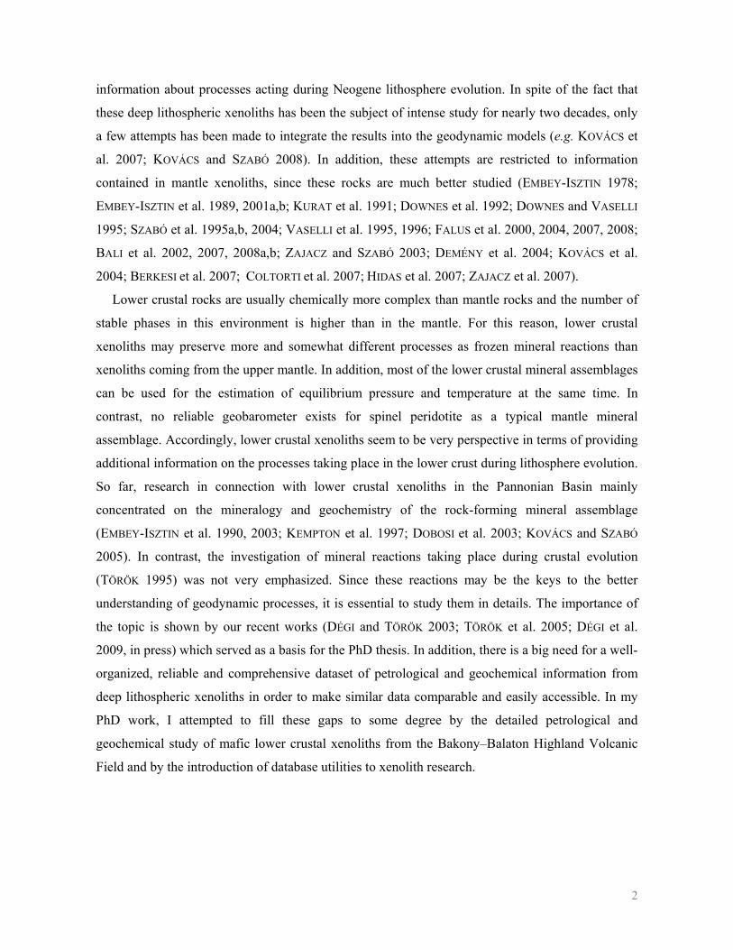
The Pannonian Basin is an area built up by a system of smaller basins and local highs enclosed
by the chains of the Southern and Eastern Alps, the Western, Eastern and Southern Carpathians and
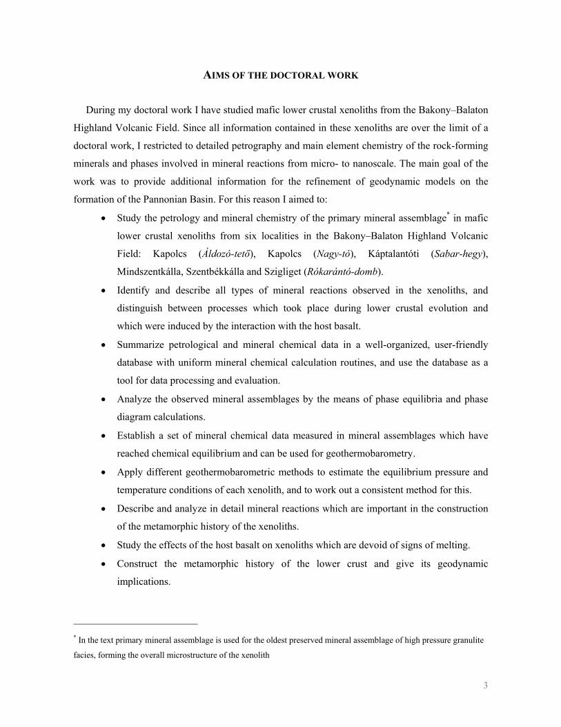
the Dinarides (Fig 1). It is characterized by 25–30 km thick crust (e.g. POSGAY et al. 1991;
HORVÁTH et al. 2005; Fig 2) and 60–70 km thick lithosphere (e.g. HORVÁTH et al. 2005). This is
associated with extremely high heat flux (e.g. DÖVÉNYI and HORVÁTH 1988; DÖVÉNYI 1994;
LENKEY 1999), which is typical for young extensional basins. The substratum of the Pannonian
Basin is composed of two major blocks (Fig 1), the ALCAPA block of African affinity in the north
and the TISZA-DACIA block of European affinity in the south (e.g. GÉCZY 1973; VÖRÖS 1993;
SZENTE 1995). These tectonic units are separated by the Mid-Hungarian Zone (MHZ; CSONTOS and
NAGYMAROSY 1998). All authors agree in that the juxtaposition of major blocks and the extension
of the basin is the result of continuous overall convergence of Africa and Europe in the Tertiary and
Quaternary, but some parts of the geodynamic models are still questions of debate.
Fig 1 Topography of the Pannonian Basin and the surroundings (ZENTAI 1996). Major tectonic units and shear zones taken from CSONTOS (1995) are also indicated.
5
Fig 2 Thickness of the crust in the Pannonian Basin and its surroundings (HORVÁTH et al. 2005). Red and gray lines mark the places of continent-continent collision and country borders, respectively.
I.1 Tertiary geodynamics of the Pannonian Basin
The Paleogene evolution of the Mediterranean region was determined by the northward drift and
counterclockwise rotation of the Apulian microcontinent of African origin (RING et al. 1989). This
motion was accompanied by the consumption of two oceans characterized by old oceanic
lithosphere: the Penninic ocean, located north of Apulia, (CSONTOS 1995; CHANNELL and KOZUR
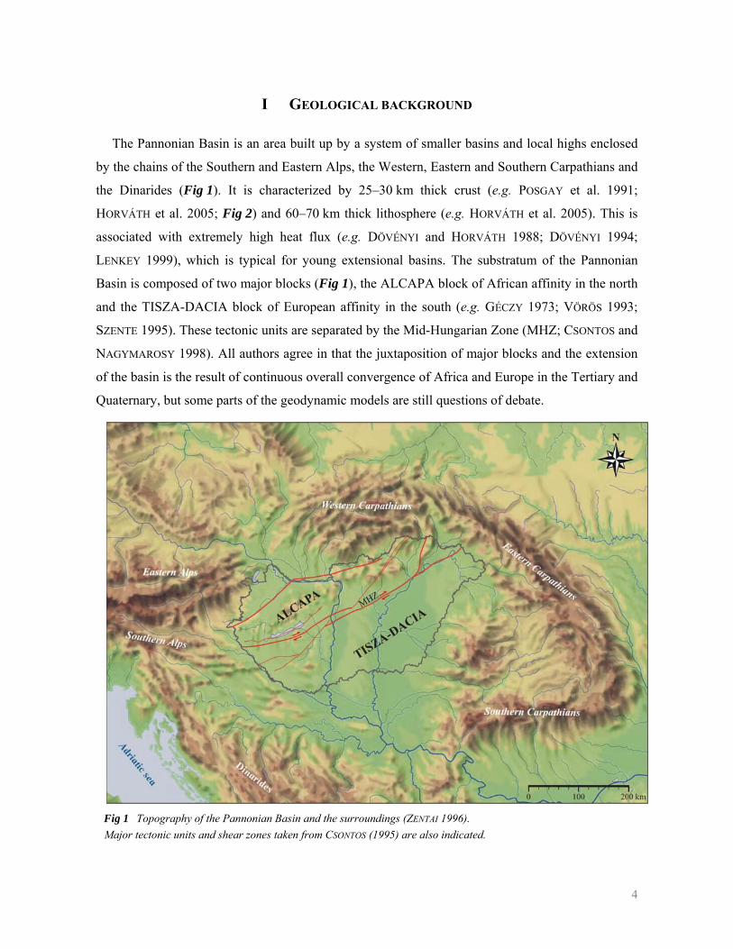
1997; NEMCOK et al. 1998) and the Budva-Pindos ocean (CSONTOS and VÖRÖS 2004) on the
eastern margin of the microcontinent (Fig 3). The Penninic ocean subducted southward beneath
Apulia. At the same time, the subduction of the Budva-Pindos ocean dipped northeastward
(LIPPITSCH et al. 2003). According to KOVÁCS et al. (2007), a continuous volcanic arc existed along
the subduction front of the Budva-Pindos ocean in the Eocene and Early Oligocene. The Paleogene
andesitic volcanic rocks found in the present day Southern Alps, Dinaric region and along the Mid-
Hungarian Zone were probably generated in this volcanic arc (KOVÁCS and SZABÓ 2008). Based on
the fits of Mesozoic facies provinces, KÁZMÉR and KOVÁCS (1985) have suggested that the
ALCAPA unit in this period was positioned near the Drauzug in the Eastern Alps, which was not
far from the northern part of the Budva-Pindos subduction front (KOVÁCS and SZABÓ 2008).
6
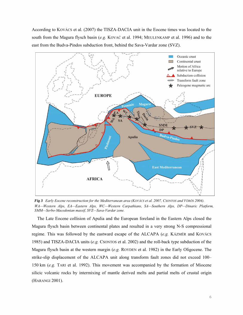
According to KOVÁCS et al. (2007) the TISZA-DACIA unit in the Eocene times was located to the
south from the Magura flysch basin (e.g. KOVAĆ et al. 1994; MEULENKAMP et al. 1996) and to the
east from the Budva-Pindos subduction front, behind the Sava-Vardar zone (SVZ).
Fig 3 Early Eocene reconstruction for the Mediterranean area (KOVÁCS et al. 2007, CSONTOS and VÖRÖS 2004). WA—Western Alps, EA—Eastern Alps, WC—Western Carpathians, SA—Southern Alps, DP—Dinaric Platform, SMM—Serbo-Macedonian massif, SVZ—Sava-Vardar zone.
The Late Eocene collision of Apulia and the European foreland in the Eastern Alps closed the
Magura flysch basin between continental plates and resulted in a very strong N-S compressional
regime. This was followed by the eastward escape of the ALCAPA (e.g. KÁZMÉR and KOVÁCS
1985) and TISZA-DACIA units (e.g. CSONTOS et al. 2002) and the roll-back type subduction of the
Magura flysch basin at the western margin (e.g. ROYDEN et al. 1982) in the Early Oligocene. The
strike-slip displacement of the ALCAPA unit along transform fault zones did not exceed 100–
150 km (e.g. TARI et al. 1992). This movement was accompanied by the formation of Miocene
silicic volcanic rocks by intermixing of mantle derived melts and partial melts of crustal origin
(HARANGI 2001).
7
Many theories exist which describe the mechanism of continental escape and its correlation with
the roll-back type subduction. Most authors (e.g. ROYDEN 1988; CSONTOS et al. 1992; FODOR et al.
1999; HUISMANS et al. 2001; HORVÁTH 2007) suggest that the ALCAPA was extruded from the
Alps as a crustal block. In contrast, some authors (e.g. WILLINGSHOFFER et al. 1999,
WILLINGSHOFFER and CLOETINGH 2003; KOVÁCS and SZABÓ 2008) argue that the extrusion
effected the whole lithospheric column. Geochemical (e.g. BALI et al. 2002, 2007, 2008a,b;
DEMÉNY et al. 2004; COLTORTI et al. 2007) and deformation studies (e.g. FALUS et al. 2000, 2004,
2008) of mantle xenoliths indicate that at least part of the lithospheric mantle was extruded together
with the crust of the ALCAPA.
According to HORVÁTH (2007), the extrusion of the ALCAPA unit as a crustal block was driven
by the N-S shortening in the Alps and the roll-back type subduction of the Magura basin. The
extruded block slipped directly onto the hot asthenospheric material left behind by the retreating
subduction front. The overthickened crustal block was heated up, which facilitated its gravitational
collapse (e.g. RATSCHBACHER et al 1991). However, KOVÁCS and SZABÓ (2008) suggest that an
E-W directed hot mantle flow was generated behind the Budva-Pindos subduction front and this
flow forced the ALCAPA unit to escape from the Eastern Alps together with its lithospheric
mantle. In addition, the mantle flow may have strengthened the steepening and retreating of the
subducting Magura slab.
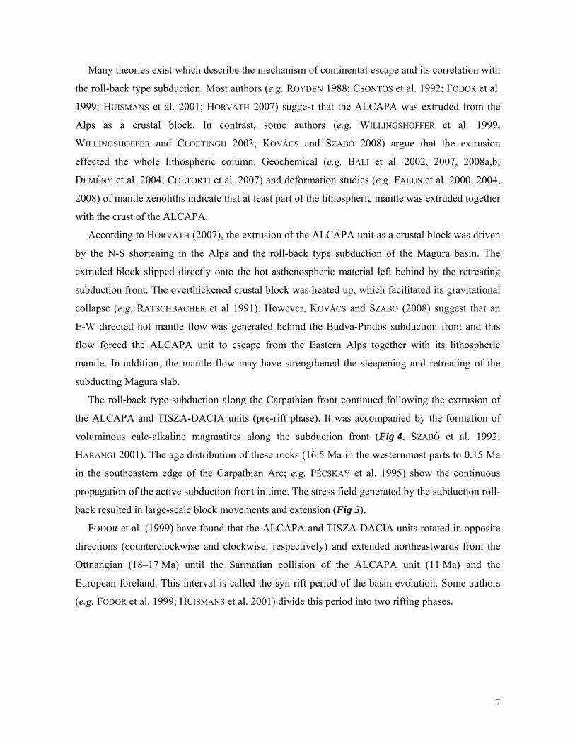
The roll-back type subduction along the Carpathian front continued following the extrusion of
the ALCAPA and TISZA-DACIA units (pre-rift phase). It was accompanied by the formation of
voluminous calc-alkaline magmatites along the subduction front (Fig 4, SZABÓ et al. 1992;
HARANGI 2001). The age distribution of these rocks (16.5 Ma in the westernmost parts to 0.15 Ma
in the southeastern edge of the Carpathian Arc; e.g. PÉCSKAY et al. 1995) show the continuous
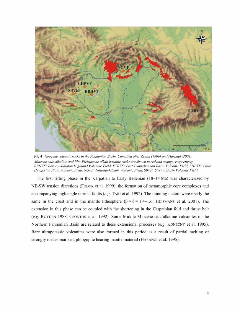
propagation of the active subduction front in time. The stress field generated by the subduction roll-
back resulted in large-scale block movements and extension (Fig 5).
FODOR et al. (1999) have found that the ALCAPA and TISZA-DACIA units rotated in opposite
directions (counterclockwise and clockwise, respectively) and extended northeastwards from the
Ottnangian (18–17 Ma) until the Sarmatian collision of the ALCAPA unit (11 Ma) and the
European foreland. This interval is called the syn-rift period of the basin evolution. Some authors
(e.g. FODOR et al. 1999; HUISMANS et al. 2001) divide this period into two rifting phases.
8
Fig 4 Neogene volcanic rocks in the Pannonian Basin. Compiled after Zentai (1996) and Harangi (2001). Miocene calc-alkaline and Plio-Pleistocene alkali basaltic rocks are shown in red and orange, respectively. BBHVF: Bakony–Balaton Highland Volcanic Field, ETBVF: East Transylvanian Basin Volcanic Field, LHPVF: Little Hungarian Plain Volcanic Field, NGVF: Nógrád–Gömör Volcanic Field, SBVF: Styrian Basin Volcanic Field.
The first rifting phase in the Karpatian to Early Badenian (18–14 Ma) was characterized by
NE-SW tension directions (FODOR et al. 1999), the formation of metamorphic core complexes and
accompanying high angle normal faults (e.g. TARI et al. 1992). The thinning factors were nearly the
same in the crust and in the mantle lithosphere (β = δ = 1.4–1.6, HUISMANS et al. 2001). The
extension in this phase can be coupled with the shortening in the Carpathian fold and thrust belt
(e.g. ROYDEN 1988; CSONTOS et al. 1992). Some Middle Miocene calc-alkaline volcanites of the
Northern Pannonian Basin are related to these extensional processes (e.g. KONEČNÝ et al. 1995).
Rare ultrapotassic volcanites were also formed in this period as a result of partial melting of
strongly metasomatized, phlogopite bearing mantle material (HARANGI et al. 1995).
9
Fig 5 Miocene evolution of the Pannonian Basin. a) Block movements (FODOR et al. 1999). b) Evolution of the lithosphere (HUISMANS et al. 2001).
10
The main tension directions have changed to E-W to SE-NW (FODOR et al. 1999) in the second
rifting phase (12–11 Ma). The central parts of the Pannonian Basin were mostly effected by these
processes (CSONTOS 1995). The thinning of the crust (β = 1.1) was insignificant as compared with
the thinning of the mantle lithosphere (δ = 4–8) in this period (HUISMANS et al. 2001). These
changes may be explained by an intense asthenospheric upwelling, which resulted in the formation
of a mantle diapir intensely eroding the lithospheric mantle (e.g. STEGENA et al. 1975; HUISMANS et
al. 2001). This was followed by sporadic alkali basaltic volcanism in the Pliocene–Pleistocene
times (Fig 4, EMBEY-ISZTIN et al. 1993).
The Sarmatian collision of the ALCAPA and later the TISZA-DACIA units (11–8 Ma) with the
European foreland led to a compression event, the Post-Sarmatian tectonic inversion (e.g. CSONTOS
et al. 1992) which is regarded as the end of extension in the Pannonian Basin. This was followed by
the post-rift thermal subsidence of the basin, the accumulation of voluminous alluvial sediments
parallel with the steepening of the subducted slab beneath the fixed subduction front (e.g. HORVÁTH
1995). The detachment of the subducting slab nearly perpendicular to the surface resulted in a new
compression event in the Pliocene which is determining the present day tectonics of the region (e.g.
HORVÁTH and CLOETINGH 1996; BADA et al. 1999, 2007; FODOR et al. 2005; HORVÁTH et al.
2005).
I.2 Xenolith-bearing volcanism in the Pannonian Basin
Deep lithospheric xenoliths in the Pannonian Basin were found in Late Miocene–Quaternary
post-extensional mafic volcanic rocks (e.g. EMBEY-ISZTIN et al. 1993) and in Cretaceous
lamprophyres (e.g. SZABÓ et al. 1993; DOWNES et al. 1995a; NÉDLI and M. TÓTH 2007). The
processes which acted during the Miocene lithosphere evolution may only seen in xenoliths uplifted
by post-extensional volcanics.
The mantle diapir formed during the second rifting phase of the extension of the Pannonian
Basin resulted in xenolith-bearing alkali basaltic volcanism in five areas: Styrian Basin, Little
Hungarian Plain, Bakony–Balaton Highland, Nógrád–Gömör and East Transylvanian Basin
Volcanic Fields (Fig 4, EMBEY-ISZTIN et al. 1993). Olivine tholeiites, alkali basalts and basanites
occur in the Little Hungarian Plain and in the Bakony–Balaton Highland Volcanic Field (BBHVF),
nephelinites are found in the Styrian Basin and basanites characterize the Nógrád–Gömör and East
Transylvanian Basin Volcanic Fields (EMBEY-ISZTIN et al. 1990). The volcanism began first 12–
10 Ma (e.g. BALOGH et al. 1986, 1994) in the western part of the Little Hungarian Plane. The
volcanic activity culminated 5–3 Ma in all volcanic fields. The last eruptions yielding deep
lithospheric xenolith-bearing volcanics occurred around 0.7 Ma in the East Transylvanian Basin
11
Volcanic Field (e.g. DOWNES et al. 1995b). Major element composition of the melts implies that
they represent mantle derived primary magmas (EMBEY-ISZTIN et al. 1993). Partial melting
occurred at 80 – 100 km mantle depth, in the garnet stability zone (EMBEY-ISZTIN and DOBOSI
1995; HARANGI et al. 1995). Trace element compositions indicate subduction related component in
the source region of most of the magmas (e.g. DOWNES et al. 1995b; HARANGI 2001, GMÉLING et
al. 2007).
The studied xenoliths originate from the Bakony–Balaton Highland Volcanic Field (Fig 6),
which is located in the centre of the Pannonian Basin (Fig 4). This part of the basin was effected by
extensional tectonics most intensely (CSONTOS 1995). The volcanic field is built up by more than
200 volcanic centres, which are located mostly at the northern shore of the Lake Balaton from
Szigliget to Tihany and in the southern part of the Bakony Mts. Phreatomagmatic to magmatic
eruptions characterized the volcanism resulting in various volcanic forms (e.g. HARANGI and
HARANGI 1995; NÉMETH and MARTIN 1999a,b). According to 40Ar/39Ar measurements, the
volcanic activity took place in two broad periods, the Tihany and Hegyestű volcanoes were formed
7.9–8.0 million years ago while the rest of the volcanic centres were active in the second period,
5.5–2.6 million years ago (WIJBRANS et al. 2007). Large amounts of xenoliths were brought to the
surface by the basaltic volcanism. The entire lithospheric column was sampled including material
from the upper mantle, as well as lower, middle and upper crustal xenoliths.
I.3 Crustal xenoliths in the BBHVF
Volcanics of the BBHVF contain several types of crustal xenoliths (Fig 6) besides ultramafic
rocks of upper mantle origin. Fragments of the upper crust are presented by low grade Paleozoic
metamorphic rocks (phyllites, quartzites, crystalline limestones), Permian sandstones and rhyolites,
Mesozoic carbonates and Pliocene sandstones (TÖRÖK et al. 2005). Clinopyroxene–plagioclase
felses (Cpx–Pl felses), buchites and some felsic granulites represent the middle crust (e.g. TÖRÖK
2002; NÉMETH et al. 2009). Lower crustal xenoliths are dominated by mafic granulites (EMBEY-
ISZTIN et al. 1990, 2003; TÖRÖK 1995; KEMPTON et al. 1997; DOBOSI et al. 2003; DÉGI and TÖRÖK
2003; TÖRÖK et al. 2005; DÉGI et al. 2009, in press), but metasedimentary granulites (EMBEY-
ISZTIN et al. 2003), high pressure Cpx–Pl felses (K. TÖRÖK, personal communication) and garnet–
orthopyroxene–plagioclase felses (Grt–Opx–Pl felses) (TÖRÖK et al. 2007) are also found in small
amounts.
12
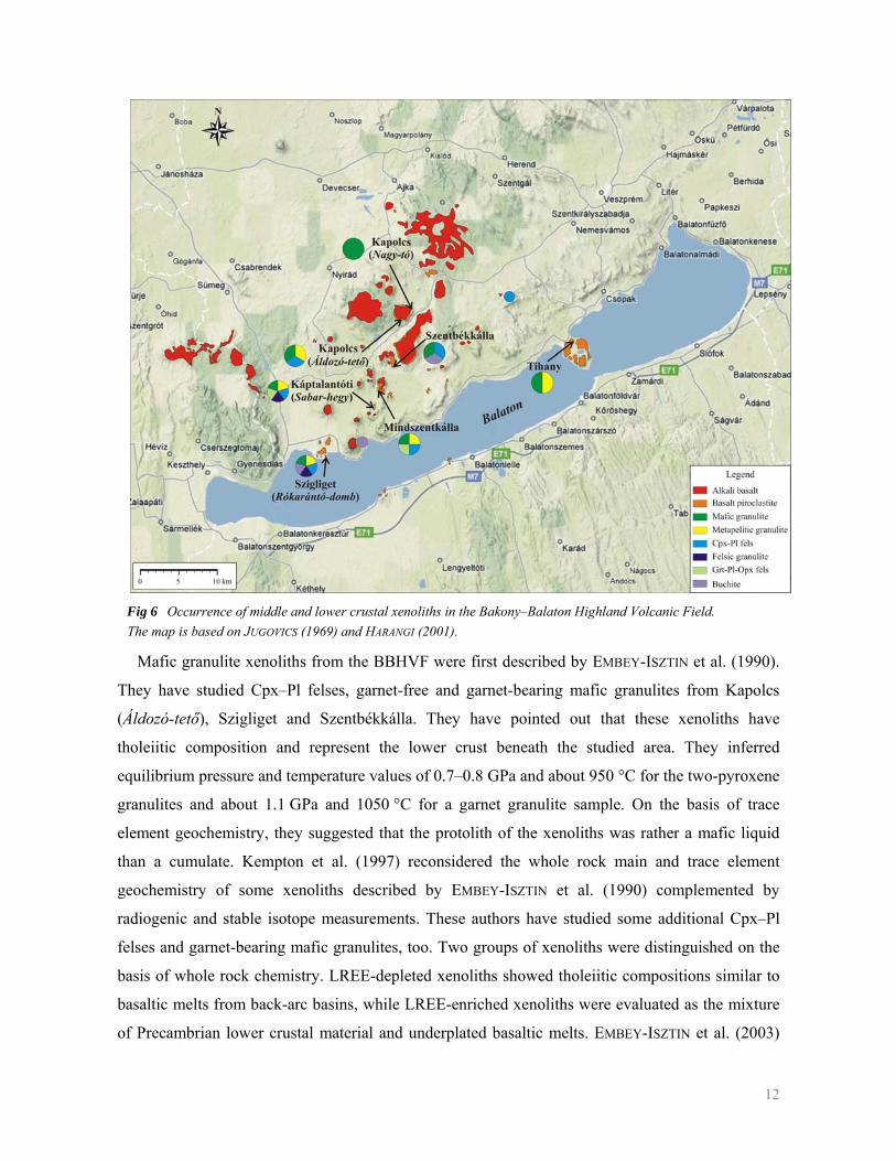
Fig 6 Occurrence of middle and lower crustal xenoliths in the Bakony–Balaton Highland Volcanic Field. The map is based on JUGOVICS (1969) and HARANGI (2001).
Mafic granulite xenoliths from the BBHVF were first described by EMBEY-ISZTIN et al. (1990).
They have studied Cpx–Pl felses, garnet-free and garnet-bearing mafic granulites from Kapolcs
(Áldozó-tető), Szigliget and Szentbékkálla. They have pointed out that these xenoliths have
tholeiitic composition and represent the lower crust beneath the studied area. They inferred
equilibrium pressure and temperature values of 0.7–0.8 GPa and about 950 °C for the two-pyroxene
granulites and about 1.1 GPa and 1050 °C for a garnet granulite sample. On the basis of trace
element geochemistry, they suggested that the protolith of the xenoliths was rather a mafic liquid
than a cumulate. Kempton et al. (1997) reconsidered the whole rock main and trace element
geochemistry of some xenoliths described by EMBEY-ISZTIN et al. (1990) complemented by
radiogenic and stable isotope measurements. These authors have studied some additional Cpx–Pl
felses and garnet-bearing mafic granulites, too. Two groups of xenoliths were distinguished on the
basis of whole rock chemistry. LREE-depleted xenoliths showed tholeiitic compositions similar to
basaltic melts from back-arc basins, while LREE-enriched xenoliths were evaluated as the mixture
of Precambrian lower crustal material and underplated basaltic melts. EMBEY-ISZTIN et al. (2003)
13
and DOBOSI et al. (2003) described garnet-bearing granulites from two new localities,
Mindszentkálla and Káptalantóti (Sabar-hegy). On the basis of new mineral chemical data, whole
rock major and trace element chemistry and stable isotope composition, they reinterpreted the
nature and origin of the lower crust in the region. They estimated the equilibration pressure and
temperature of the xenoliths to 1.0–1.4 GPa and 800–1000 °C which is consistent with a 40 km
thick Alpine crust. On the basis of rare earth elements (REE), Sr, Hf, Nd and O isotopic analysis,
they assumed that the precursor of the garnet granulites may have been oceanic pillow basalts,
which were the subject of granulite facies metamorphism during the Alpine orogenesis.
14
II METHODS
As it was emphasized in the introduction, previous works on lower crustal xenoliths from the
BBHVF mainly concentrated on the whole rock chemistry of the xenoliths and the mineral
chemistry of the rock-forming minerals. Although mineral reactions occurring in the xenoliths are
very important in understanding the metamorphic evolution of the rock, they were not studied in
details until now. My PhD work would like to provide the basis of these kinds of investigations. In
this section I describe the research strategy I followed (Section II.1) and the applied analytical
techniques (Section II.2).
II.1 Research strategy
The investigation of processes that acted during the metamorphic evolution of a rock requires
the combination of detailed petrography and chemistry of the rock-forming minerals and phases
involved in mineral reactions from micro- to nanoscale. In this work I restricted the mineral
chemistry to the main element composition, otherwise it would exceed the limits of a PhD thesis.
During my investigations I followed the strategy described below.
As a first step, I described the xenoliths macroscopically. I identified mineral phases and
macroscopic characteristics, which were observable by naked eye, such as banded structure or
degree of weathering. From most of the samples, 30 – 40 μm thick thin sections were made. I
studied the thin sections by optical microscopy both in transmitted and reflected light to describe
microscopic features of the samples. After the identification of the phases, I distinguished mineral
assemblages and I tried to establish their relative formation sequence according to microstructural
observations. I classified the samples on the basis of petrology and chose the representative ones
for further analysis.
The representative samples were analyzed in conventional electron microprobe. I checked the
homogeneity of the phases by back-scattered electron imaging, qualitative line analyses and
element distribution maps. I measured the composition of the phases by electron probe
microanalysis (quantitative point analysis). If compositional zoning was detected, qualitative
element distributions acquired from line analysis and element maps were calibrated utilizing a
series of quantitative point analysis. In case of fine-grained reaction products, I refined my
microstructural observations by the combination of these methods. Since the spatial resolution
achievable by a conventional microprobe is not greater than 0.5 μm, I investigated submicron-sized
microstructures in a microprobe equipped with a field emission gun electron source (FE-EPMA). In
15
case of one extremely fine-grained mineral assemblage, the 100 nm lateral resolution achievable
with FE-EMPA was not enough for microstructural analysis. At this point, 15 μm × 10 μm ×
100 nm electron-transparent thin foils were cut from the thin section utilizing focused ion beam
(FIB) sample preparation. The nanostructure and nanoscale element distributions of the mineral
assemblage were studied using Transmission Electron Microscopy (TEM). Technical details and
descriptions of the instruments used are found in Section II.2 below.
357 thin sections from 278 xenoliths were studied. 67 thin sections were chosen for further
analysis, where 5083 quantitative point analyses in 1135 phases, 435 back-scattered electron
images (BSEI), 59 line analyses, 49 element maps and 6 TEM foils were made. The extremely
large amount of data was hardly tractable on an individual basis. This is why I organized all
obtained information in a Microsoft Access database called GRANULITE, which is described in
details in Section III. In order to make these data comparable with different types of deep
lithospheric rocks from all over the world, I constructed the Deep Lithosphere DataBase which is
available on the internet: http://lrg-dldb.elte.hu.Using the GRANULITE database, I combined
petrographical and chemical observations obtained in optical microscope and in conventional
electron microprobe in Section IV in order to distinguish different mineral assemblages in the
xenoliths. Following this, I estimated the formation conditions of the observed mineral assemblages
(Section V). As a first approximation, I defined the stability field of different mineral assemblages
on the basis of mineral equilibria and phase diagram calculations (Sections V.1 and V.2). This was
followed by geothermobarometric investigations (Section V.3). For every mineral assemblage, I
tested the state of equilibrium (Section V.3.1). Using the dataset from the primary rock-forming
mineral assemblages, I compared different geothermobarometric methods in order to find the ones
best describing the studied samples (Sections V.3.2 and V.3.3). These methods were applied for all
mineral assemblages in order to keep the results comparable.
After clarifying the equilibration conditions of the primary mineral assemblage, I studied two
mineral assemblages in detail (Sections VI and VII) in order to learn more about processes acting
in the lower crust and during the xenolith – host basalt interaction. This included advanced
petrography and mineral chemistry using high resolution analytical techniques, thermodynamic
analysis of the processes by phase diagram calculations and estimating the time scales by modelling
solid state diffusion-controlled processes.
All results were put together to construct the metamorphic evolution of the studied xenoliths
(Section VIII). This reflects the evolution of the lower crust during the formation of the Pannonian
Basin. Thus, it has important geodynamic consequences.
16
II.2 Analytical techniques
II.2.1 Scanning Electron Microscopy and Electron Probe Microanalysis
Microprobe measurements were carried out in four different laboratories: at the Eötvös
University, Budapest on an AMRAY 1810I microprobe equipped with EDS detector; at the United
States Geological Survey (USGS) Reston Headquarters on a JEOL 8900 microprobe equipped with
WDS detectors, at the University of Vienna on a Cameca SX-100 microprobe equipped with WDS
detectors and at the Free University Berlin on a JEOL JXA-8200 Superprobe equipped with WDS
detectors.
Conventional microprobe measurements were complemented by high resolution investigations
using a Field Emission Electron Probe Microanalyzer (FE-EPMA), because the field emission
electron source produces an extremely narrow and bright electron beam (CREWE et al. 1968). This
makes it possible to reduce the beam diameter to 20 nm. At the same time, the sample current is
increasing, so the acceleration voltage can be reduced to 1 kV keeping fairly good signal intensity.
Monte Carlo simulations reveal that the size of the activation volume is drastically reduced by
using this technique, and 100 nm lateral distribution is achievable (e.g. REED 2005). Measurements
were made at the GFZ German Research Centre for Geosciences, Helmholtz Centre Potsdam in
Potsdam using a JEOL thermal field emission type electron-probe JXA-8500F (HYPERPROBE).
II.2.1.1 Point analyses
Point analyses were made in all four conventional microprobe laboratories described above. In
every case, 15 kV was applied as acceleration voltage in the electron gun, and the sample current
was set to 20 nA. Pyroxene, garnet, titanite and Fe–Ti-oxide grains were measured using the
smallest possible beam diameter, while 2 μm was used for biotite, amphibole and 5 μm for
plagioclase and scapolite analyses to avoid the loss of Na. Natural standards used for the analysis of
Fe–Ti-oxides included magnetite, ilmenite, spinel and chromite from the Smithsonian standard set
(JARSOSEWICH et al. 1980). In case of the silicates, standards used included natural clinopyroxene,
orthopyroxene, andalusite, garnet, kaersutite, hornblende, phlogopite, F-Cl-apatite and barite. ZAF
corrections (ARMSTRONG 1991, 1995) were used for the calculation of oxide concentrations. Some
grains were analyzed in different laboratories. The measurement results gave fairly good
correspondence.
II.2.1.2 Semiquantitative line analyses
Line analyses were taken at the Free University Berlin by using a stage-scanning mode with a
step size of approximately 0.2 μm, a dwell time of 300 ms per pixel, and the same acceleration
voltage and sample current as for the quantitative analyses. Following background subtraction, the
17
results of line analyses were evaluated in the same way as for quantitative analyses by using the
same standards. In addition, quantitative point analyses were made on at least 3 points of a line
analysis to verify the results.
II.2.1.3 Element mapping
Part of the element distribution maps were produced at Free University Berlin using an
acceleration voltage of 15 kV and a beam current of 20 nA in WDS mode. We applied 0.20 – 0.25
micron step size and 100 ms dwell time for element mapping in stage scanning mode.
High spatial resolution element distribution maps were prepared at the GFZ German Research
Centre for Geosciences, Helmholtz Centre Potsdam in Potsdam in WDS mode. An acceleration
voltage of 8 kV, a beam current of 30 nA, stage scanning mode, and dwell times between 100 ms
and 400 ms per pixel were applied. A liquid nitrogen trap was used to minimize surface
contamination during mapping.
II.2.2 Transmission Electron Microscopy
TEM investigations were performed at the GFZ German Research Centre for Geosciences,
Helmholtz Centre Potsdam in Potsdam using a FEI TecnaiTM G2 F20 X-Twin transmission electron
microscope with a FEG electron source. The TEM is equipped with a Fishione high angle annular
dark field detector, an EDAX energy dispersive X-ray spectroscopy system and a Gatan Tridiem
(EELS, EFTEM). TEM foils were prepared on a FIB2000 instrument at the same institute.
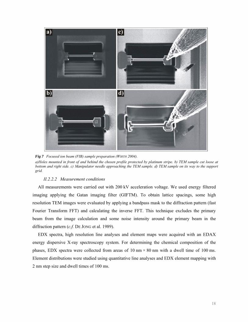
II.2.2.1 Sample preparation by using Focussed Ion Beam (FIB) technique
This technique is designed for microstructural investigations, where the exact place of sampling
should be well known. A 15 μm long and 100 nm wide platinum stripe is deposited on the surface
of the thin section exactly at the point, which has been previously marked (Fig 7). Then the surface
is bombarded with a focused beam of gallium ions, to mount a 10 μm deep hole into the thin
section in front of and behind the platinum stripe. The hole in front is big enough to make it
possible to remove the thin foil using a special manipulator system, after the thinning and polishing
of the surface by gallium ions. Details of the sample preparation process are described in WIRTH
(2004).
18
Fig 7 Focused ion beam (FIB) sample preparation (WIRTH 2004). a)Holes mounted in front of and behind the chosen profile protected by platinum stripe. b) TEM sample cut loose at bottom and right side. c) Manipulator needle approaching the TEM sample. d) TEM sample on its way to the support grid.
II.2.2.2 Measurement conditions
All measurements were carried out with 200 kV acceleration voltage. We used energy filtered
imaging applying the Gatan imaging filter (GIFTM). To obtain lattice spacings, some high
resolution TEM images were evaluated by applying a bandpass mask to the diffraction pattern (fast
Fourier Transform FFT) and calculating the inverse FFT. This technique excludes the primary
beam from the image calculation and some noise intensity around the primary beam in the
diffraction pattern (c.f. DE JONG et al. 1989).
EDX spectra, high resolution line analyses and element maps were acquired with an EDAX
energy dispersive X-ray spectroscopy system. For determining the chemical composition of the
phases, EDX spectra were collected from areas of 10 nm × 80 nm with a dwell time of 100 ms.
Element distributions were studied using quantitative line analyses and EDX element mapping with
2 nm step size and dwell times of 100 ms.
19
III DOCUMENTATION AND DATA PROCESSING — THE GRANULITE DATABASE
In the last decade, nearly 500 mafic lower crustal xenoliths were collected from the BBHVF by
the members of the Lithosphere Fluid Research Group (LRG). Different parts of the collection were
described in Theses for the National Scientific Conference of Students (BADENSZKI 2004;
KODOLÁNYI 2004), in MSc Theses (DÉGI 2004; KODOLÁNYI 2005; BADENSZKI 2006) and in this
work. All together 5083 quantitative point analyses were produced by four authors from the LRG in
the last ten years. Besides this, several types of measurement results, images and large amount of
descriptive information were produced. During my doctoral work, I aimed to collect together and
reorganize existing data in order to make them comparable and easily tractable. The large amount
of data made necessary to establish a database, since conventional spreadsheets over a few hundred
data rows become untreatable and difficult to see through. For this reason, I created the
GRANULITE database in Microsoft Access as programming platform. All data used up in this
study are summarized in the GRANULITE database. My intention was to create a well-organized
dataset, where not only numerical data, but different types of information (e.g. petrographic
description, images, line analyses) and logical relationships between the data are also included. In
addition, I aimed to perform routine mineral chemical calculations automatically in the database
and to provide such an output which is easily transferable to other calculation environments, e.g.
MS Excel spreadsheets. It was also an important aim to make the programme user-friendly so that it
could be used by people without any background in database programming. For this reason, I
constructed several forms and macros in the database. They inform the users about the different
applications of the database and lead them through the steps of each application.
The GRANULITE database consists of more than 60 tables containing more than 200 fields. In
addition, over 300 other objects (queries, forms and macros) providing various applications and
user-friendly functioning are included in the database. For this reason, a complete program
description would exceed the limits of the thesis. In the followings, I will briefly describe the data
structure (Section III.1) which assures proper documentation, and gives the basis of built-in
calculations (Section III.2) and data processing (Section III.3), such as analysis of mineral
chemical data and data preparation for geothermobarometric calculations. Finally I show a possible
extension of the GRANULITE database, the web-based Deep Lithosphere DataBase (DLDB,
Section III.4), which may serve as a platform for comparing mineral chemistry and
geothermobarometry in deep lithospheric rocks from all over the world.
20
III.1 Data structure
The GRANULITE database to a first approximation was exclusively designed for the aims of
this PhD thesis, but in a longer term it should host all requirements in connection with lower crustal
xenoliths. Unlimited number of additional data types, such as trace element geochemistry or fluid
inclusion data, should be possible to store and process in the database without significant change in
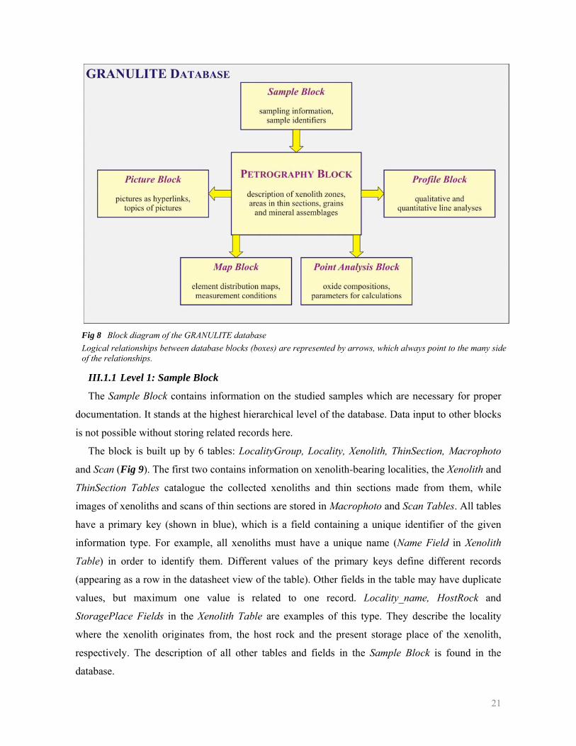
the structure of existing data. For this reason, the database has block structure (Fig 8, Appendix 1).
It is built up by six units: Sample, Petrography, Point analysis, Profile, Map and Picture Blocks.
Each block consists of tables connected by logical relationships and describes a distinct information
type. Besides numerical data, many descriptive information (e.g. measurement conditions) and
additional data necessary for calculations and further data analysis are stored in each block. As a
result of the block structure, the database is easy to complement with arbitrary number of new
information types as new blocks.
Logical relationships within and between the blocks result in a hierarchical data structure. The
Sample Block stands at the highest hierarchical level of the database. It is connected to the
Petrography Block, which represents the second hierarchical level. The other four blocks, namely
Point analysis, Profile, Map and Picture Blocks, are coequal and they are all connected to the
Petrography Block. These blocks form the third hierarchical level. Since data hierarchy is forced,
the input of measurement results is possible only if related sample information and petrography is
stored in the database. Proper documentation is assured this way. In addition, another fundamental
requirement in modern petrology is also fulfilled by the data structure. Petrographical information
is stored and treated together with the results of all types of measurements, since all information in
the database is linked through the Petrography Block (Fig 8).
The complete database consists of more than 60 tables, and more than 70 logical relationships
between them. This determines the structure of the database, referred to as topology. A simplified
topology containing the 25 most important tables and their relationships is shown in Appendix 1.
As it is seen, some tables (e.g. Campaign Table), referred to as master tables, are not parts of
blocks. They contain parameters, which may be related to more than one block, e.g. date and place
of a microprobe campaign in which quantitative point analyses, line analyses and maps were also
done.
In the followings I describe the most important features of each block and their connections to
master tables and other blocks. Detailed description of the tables and their fields is found in the
programme documentation, which is attached to the thesis electronically together with the database
file.
21
Fig 8 Block diagram of the GRANULITE database Logical relationships between database blocks (boxes) are represented by arrows, which always point to the many side of the relationships.
III.1.1 Level 1: Sample Block
The Sample Block contains information on the studied samples which are necessary for proper
documentation. It stands at the highest hierarchical level of the database. Data input to other blocks
is not possible without storing related records here.
The block is built up by 6 tables: LocalityGroup, Locality, Xenolith, ThinSection, Macrophoto
and Scan (Fig 9). The first two contains information on xenolith-bearing localities, the Xenolith and
ThinSection Tables catalogue the collected xenoliths and thin sections made from them, while
images of xenoliths and scans of thin sections are stored in Macrophoto and Scan Tables. All tables
have a primary key (shown in blue), which is a field containing a unique identifier of the given
information type. For example, all xenoliths must have a unique name (Name Field in Xenolith
Table) in order to identify them. Different values of the primary keys define different records
(appearing as a row in the datasheet view of the table). Other fields in the table may have duplicate
values, but maximum one value is related to one record. Locality_name, HostRock and
StoragePlace Fields in the Xenolith Table are examples of this type. They describe the locality
where the xenolith originates from, the host rock and the present storage place of the xenolith,
respectively. The description of all other tables and fields in the Sample Block is found in the
database.
22
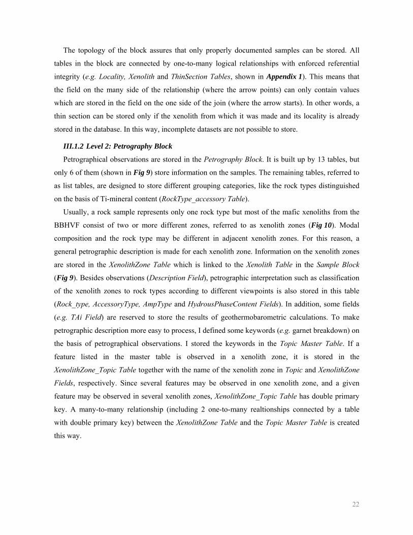
The topology of the block assures that only properly documented samples can be stored. All
tables in the block are connected by one-to-many logical relationships with enforced referential
integrity (e.g. Locality, Xenolith and ThinSection Tables, shown in Appendix 1). This means that
the field on the many side of the relationship (where the arrow points) can only contain values
which are stored in the field on the one side of the join (where the arrow starts). In other words, a
thin section can be stored only if the xenolith from which it was made and its locality is already
stored in the database. In this way, incomplete datasets are not possible to store.
III.1.2 Level 2: Petrography Block
Petrographical observations are stored in the Petrography Block. It is built up by 13 tables, but
only 6 of them (shown in Fig 9) store information on the samples. The remaining tables, referred to
as list tables, are designed to store different grouping categories, like the rock types distinguished
on the basis of Ti-mineral content (RockType_accessory Table).
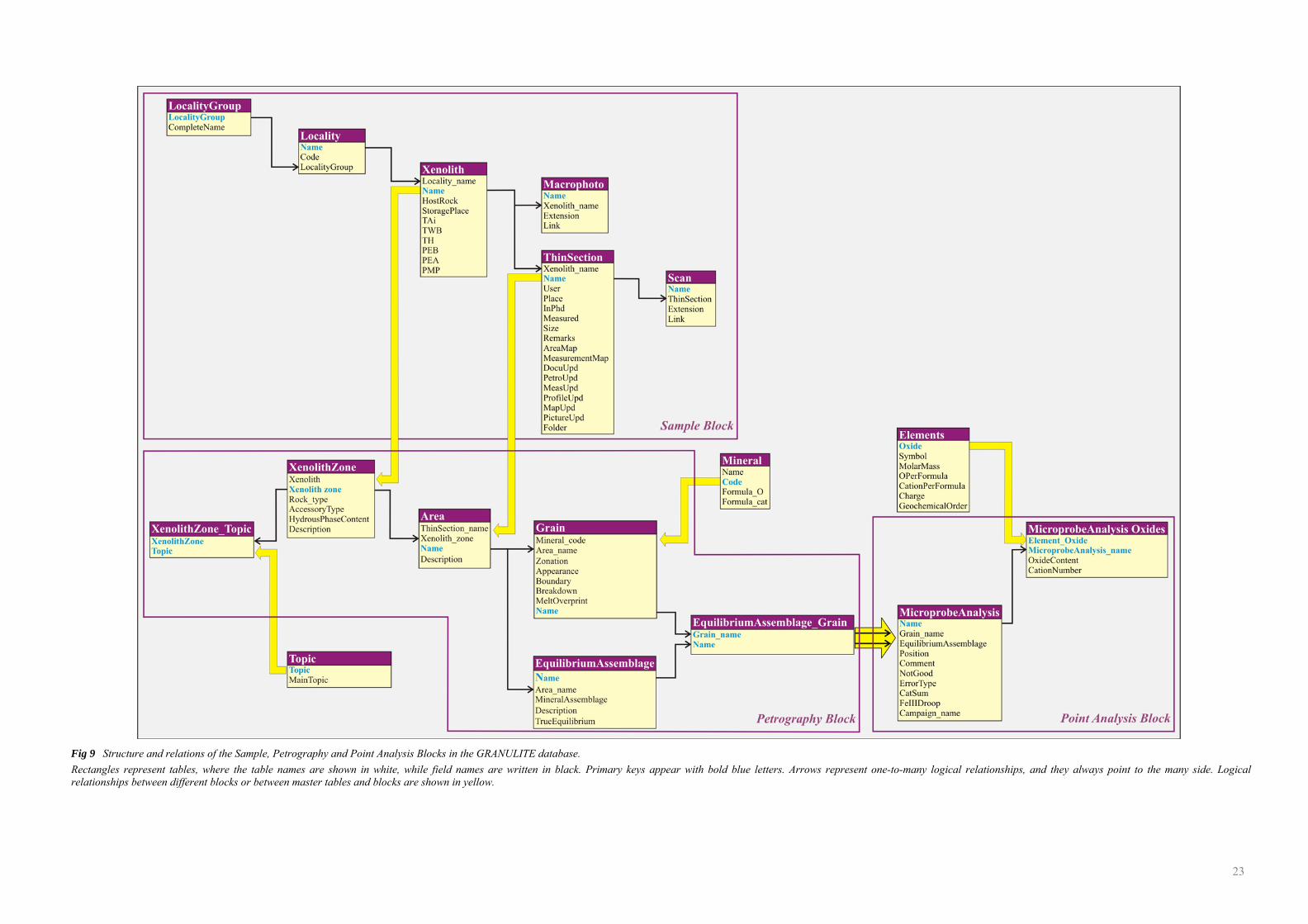
Usually, a rock sample represents only one rock type but most of the mafic xenoliths from the
BBHVF consist of two or more different zones, referred to as xenolith zones (Fig 10). Modal
composition and the rock type may be different in adjacent xenolith zones. For this reason, a
general petrographic description is made for each xenolith zone. Information on the xenolith zones
are stored in the XenolithZone Table which is linked to the Xenolith Table in the Sample Block
(Fig 9). Besides observations (Description Field), petrographic interpretation such as classification
of the xenolith zones to rock types according to different viewpoints is also stored in this table
(Rock_type, AccessoryType, AmpType and HydrousPhaseContent Fields). In addition, some fields
(e.g. TAi Field) are reserved to store the results of geothermobarometric calculations. To make
petrographic description more easy to process, I defined some keywords (e.g. garnet breakdown) on
the basis of petrographical observations. I stored the keywords in the Topic Master Table. If a
feature listed in the master table is observed in a xenolith zone, it is stored in the
XenolithZone_Topic Table together with the name of the xenolith zone in Topic and XenolithZone
Fields, respectively. Since several features may be observed in one xenolith zone, and a given
feature may be observed in several xenolith zones, XenolithZone_Topic Table has double primary
key. A many-to-many relationship (including 2 one-to-many realtionships connected by a table
with double primary key) between the XenolithZone Table and the Topic Master Table is created
this way.
23
Fig 9 Structure and relations of the Sample, Petrography and Point Analysis Blocks in the GRANULITE database. Rectangles represent tables, where the table names are shown in white, while field names are written in black. Primary keys appear with bold blue letters. Arrows represent one-to-many logical relationships, and they always point to the many side. Logical relationships between different blocks or between master tables and blocks are shown in yellow.
24
General petrographic description of xenolith zones can be refined in the Area, Grain and
EquilibriumAssemblage Tables (Fig 9). The Area Table has a key role in precise documentation.
Names and short descriptions of the studied areas are stored here. Each area belongs to a xenolith
zone and a thin section. Place of areas are marked on the map of the thin section in digital format
(Fig 10). This file is stored as a hyperlink in the ThinSection Table, which is linked to the Area
Table. This way the description of the area can be queried together with the hyperlink of the
graphical documentation, which can be directly opened from the database. This data structure
creates the link between graphical and descriptive documentation and assures that all information is
easy to retrieve.
The description of areas is further refined by the characterization of grains in the Grain Table
and by using pre-defined categories. In addition, local mineral assemblages formed by grains which
may be in equilibrium with each other are also named in the EquilibriumAssemblage Table. These
assemblages are categorized to generally observed mineral assemblage types (i.e. breakdown
products of amphibole) in the MineralAssemblage Field of the table. Following this, the grains
which belong to the same local mineral assemblage are documented. Since one grain may belong to
more than one mineral assemblage (e.g. a plagioclase grain with overgrowth from an infiltrating
melt), and all assemblages are built up by more than one grain, a many-to-many relationship should
be created between Grain and EquilibriumAssemblage Tables. For this reason, this information is
stored in the EquilibriumAssemblage_Grain Table with double primary key (Fig 9). This data
structure gives the basis and the essence of geothermobarometric investigations using the database.
All minerals holding local equilibrium are stored only once in the database by a user, but later
unlimited number of different equilibrium mineral assemblages and any combination of related data
(e.g. mineral composition) is found automatically in a database. This reduces drastically the time
necessary for data organizing preceding geothermobarometric calculations. Depending on the size
of the dataset, hours or days of human work is converted to seconds or minutes.
Although the data structure of the Petrography Block may look complicated, it is extremely
important to store petrographic information in an organized way. This data structure assures proper
and retrievable documentation. Graphical documentation is coupled with ‘ordinary’ descriptions
which document all the details of the observations. This is complemented by descriptions using
keywords and classification of observations to pre-defined categories. These are easy to query, so
that relationships between petrography and measurement results can be found fast. This makes data
analysis much more effective and faster and it opens new perspectives in data processing and
interpretation. The storage of grains which may formed in equilibrium with each other as parts of a
25
local mineral assemblage, creates the possibility to find mineral pairs which can be used for
geothermobarometry in a minute.
Fig 10 Xenolith zones and measured areas marked on the digital map of the Sab10 thin section.
III.1.3 Level 3: Measurement Blocks
Blocks of the third hierarchical level contain information in connection with different types of
measurements carried out in the samples. All blocks are connected to the Area Table in the
Petrography Block (Appendix 1). This assures that the places of measurements are easy to find in
the thin sections by using optical microscope. The exact position of analyses is documented
graphically in a CorelDraw file for most of the thin sections. These files are also stored in the
26
ThinSection Table as hyperlinks, so they can be opened directly from the database. Measurements
are usually made in measurement campaigns where some conditions are common in all cases. For
this reason measurements conditions are stored in the Campaign Master Table, which is linked to
all Measurement Blocks too.
The Point Analysis Block contains the results of quantitative microprobe point analyses. Features
of analyses are stored in the MicroprobeAnalysis Table, whereas numerical data are found in the
MicroprobeAnalysis_Oxides Table. Although this block consists only of 2 tables which contain
information on the samples and 4 additional list tables, most of the data are stored here. The block
has special relation with the Petrography Block (Fig 9). All analyses are related to a grain and a
local mineral assemblage. The double join with the EquilibriumAssemblage_Grain Table assures
that only pre-defined combinations are accepted. The block has logical relationships with Mineral
and Elements Master Tables, which contain parameters of built-in calculations, which are described
in more details in Section III.2. Some calculation results, which are frequently required (i.e. cation
numbers and Fe3+-content calculated by the method of Droop 1987), are stored in this block, too.
The Profile and Map Blocks were designed to store the most important information on line
analyses and element maps, respectively. This includes special measurement conditions, description
of the profile or map, measured elements and hyperlink of the folder, where measurement results
are stored. In addition, if quantitative point analyses were measured along a line, analysis names
together with the distance from the starting point can be stored in the Profile_points Table. This
makes easy to calibrate semi-quantitative line analyses.
The Picture Block is used to store descriptive information about images made in the studied
areas. The main purpose of creating this block was the categorization of images to topics without
making duplicate copies on the hard disk, since these files occupy large space. For this reason, the
Picture Table is linked to the Topic Master Table with a many-to-many relationship similar to the
join of the master table with the XenolithZone Table. This way, images can be described using
keywords also. By querying hyperlinks of images belonging to a given feature or mineral
assemblage, image analysis is integrated into the data interpretation process.
III.2 Built-in calculations in the GRANULITE database
One of the main goals of creating the GRANULITE database was to make data comparable by
using the same calculations to derive mineral chemical quantities. In addition, the large number of
data required fast, automated calculations. For this purpose, only the oxide compositions measured
in quantitative point analyses were filled in the database and all mineral chemical calculations are
carried out using queries. Three kinds of quantities are derived from the results of oxide
27
composition of minerals within the database: cation numbers, end members of minerals and
Fe2+/Fe3+ ratios according to different methods. Each calculation consists of several queries, which
are organized into query families, marked with the same word at the beginning of query names.
III.2.1 Calculation of cation numbers
The first order mineral chemical information which can be derived from oxide compositions is
the atomic proportion (or mole fraction) of cations per mineral formula unit (p.f.u.), referred to as
cation number. Formula unit is defined here by the theoretical number of anions (most commonly
O2−) in the chemical formula of the given mineral. The derivation of cation numbers is usually done
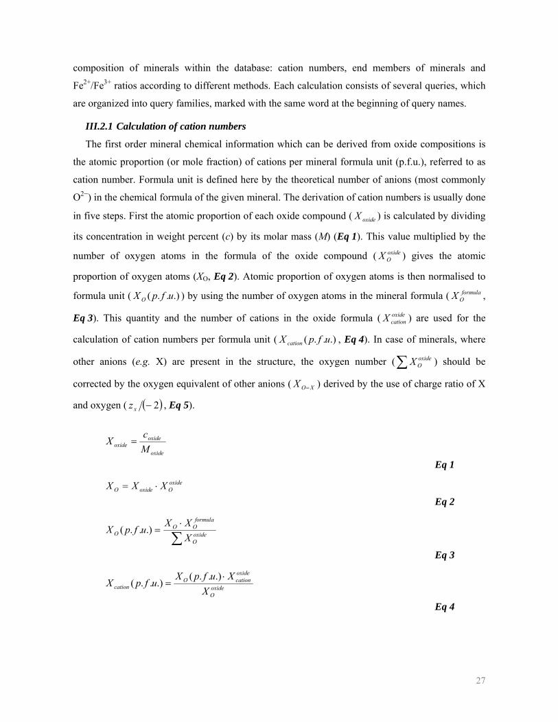
in five steps. First the atomic proportion of each oxide compound ( oxideX ) is calculated by dividing
its concentration in weight percent (c) by its molar mass (M) (Eq 1). This value multiplied by the
number of oxygen atoms in the formula of the oxide compound ( oxideOX ) gives the atomic
proportion of oxygen atoms (XO, Eq 2). Atomic proportion of oxygen atoms is then normalised to
formula unit ( .)..( ufpX O ) by using the number of oxygen atoms in the mineral formula ( formulaOX ,
Eq 3). This quantity and the number of cations in the oxide formula ( oxidecationX ) are used for the
calculation of cation numbers per formula unit ( .)..( ufpX cation , Eq 4). In case of minerals, where
other anions (e.g. X) are present in the structure, the oxygen number (∑ oxideOX ) should be
corrected by the oxygen equivalent of other anions ( XOX = ) derived by the use of charge ratio of X
and oxygen ( ( )2−xz , Eq 5).
oxide
oxideoxide M
cX =
Eq 1 oxideOoxideO XXX ⋅=
Eq 2
∑⋅
= oxideO
formulaOO
O XXX
ufpX .)..(
Eq 3
oxideO
oxidecationO
cation XXufpX
ufpX⋅
=.)..(
.)..(
Eq 4
28
2−⋅
==XO
XOzX
X
Eq 5 The above mentioned calculation methods have several disadvantages when large amount of
data should be treated. Although calculations can be written in one line in Microsoft Excel, the
order of columns is predefined and calculation formulas are applicable only for analyses, where the
same elements are listed in the same order. Since formulaOX is different for nearly all of the minerals,
analyses should be grouped by minerals and stored in different Excel sheets. Lastly, calculations for
minerals containing other anions than oxygen are never straightforward. Because of these
problems, I constructed the Cation built-in calculation query family in the database with the help of
Dr. Szabolcs Papp, lecturer at the Department of Media and Teaching Informatics, Faculty of
Informatics, Eötvös University.
Calculation parameters, which differ from mineral to mineral (such as number of oxygen atoms
per formula) and from element to element (e.g. molar mass, charge, etc.) are stored in the Mineral
and Elements Master Tables (Fig 9), respectively. Logical relationships between the Petrography
and Point Analysis Blocks make it possible to find which analysis belongs to which mineral,
although all analysis results are stored in the MicroprobeAnalysis_Oxides Table. The join between
the MicroprobeAnalysis_Oxides Table and the Elements Master Table assures that it is always
possible to match the concentration of an oxide with its molar mass, even if the order and the
analysed elements vary from analysis to analysis.
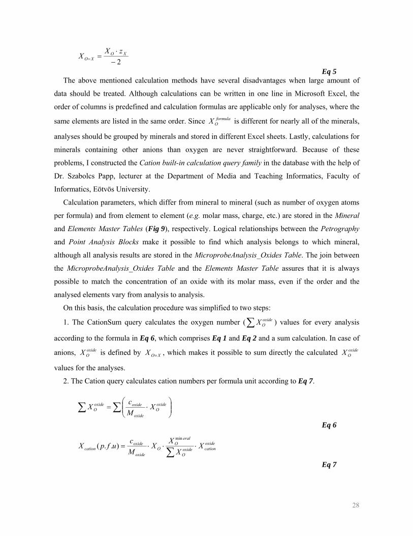
On this basis, the calculation procedure was simplified to two steps:
1. The CationSum query calculates the oxygen number (∑ oxideOX ) values for every analysis
according to the formula in Eq 6, which comprises Eq 1 and Eq 2 and a sum calculation. In case of
anions, oxideOX is defined by XOX = , which makes it possible to sum directly the calculated oxide
OX
values for the analyses.
2. The Cation query calculates cation numbers per formula unit according to Eq 7.
∑ ∑ ⎟⎟⎠
⎞⎜⎜⎝
⎛⋅= oxide
Ooxide
oxideoxideO X
Mc
X
Eq 6
oxidecationoxide
O
eralO
Ooxide
oxidecation X
XX
XMc
ufpX ⋅⋅⋅=∑
min
)..(
Eq 7
29
Cation numbers play an important role in data validation (further described in Section III.3.1)
and they are frequently used input parameters for other calculations, such as geothermobarometry.
To make the cation number-based data analysis and calculations faster, calculated cation numbers
are stored in the CationNumber Field of MicroprobeAnalysis_Oxides Table. This procedure is done
by the three other queries in the Cation built-in calculation query family.
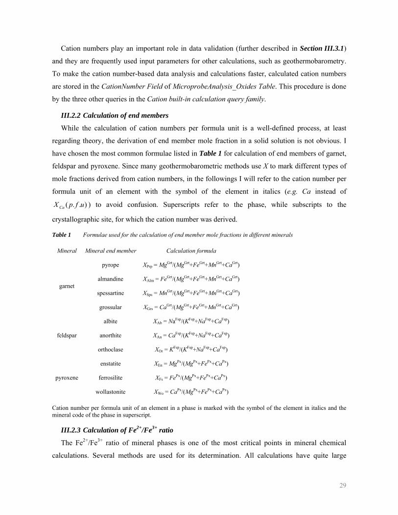
III.2.2 Calculation of end members
While the calculation of cation numbers per formula unit is a well-defined process, at least
regarding theory, the derivation of end member mole fraction in a solid solution is not obvious. I
have chosen the most common formulae listed in Table 1 for calculation of end members of garnet,
feldspar and pyroxene. Since many geothermobarometric methods use X to mark different types of
mole fractions derived from cation numbers, in the followings I will refer to the cation number per
formula unit of an element with the symbol of the element in italics (e.g. Ca instead of
)..( ufpX Ca ) to avoid confusion. Superscripts refer to the phase, while subscripts to the
crystallographic site, for which the cation number was derived.
Table 1 Formulae used for the calculation of end member mole fractions in different minerals
Mineral Mineral end member Calculation formula
pyrope XPrp = MgGrt/(MgGrt+FeGrt+MnGrt+CaGrt)
almandine XAlm = FeGrt/(MgGrt+FeGrt+MnGrt+CaGrt)
spessartine XSps = MnGrt/(MgGrt+FeGrt+MnGrt+CaGrt) garnet
grossular XGrs = CaGrt/(MgGrt+FeGrt+MnGrt+CaGrt)
albite XAb = NaFsp/(KFsp+NaFsp+CaFsp)
anorthite XAn = CaFsp/(KFsp+NaFsp+CaFsp) feldspar
orthoclase XOr = KFsp/(KFsp+NaFsp+CaFsp)
enstatite XEn = MgPx/(MgPx+FePx+CaPx)
ferrosilite XFs = FePx/(MgPx+FePx+CaPx) pyroxene
wollastonite XWo = CaPx/(MgPx+FePx+CaPx)
Cation number per formula unit of an element in a phase is marked with the symbol of the element in italics and the mineral code of the phase in superscript.
III.2.3 Calculation of Fe2+/Fe3+ ratio
The Fe2+/Fe3+ ratio of mineral phases is one of the most critical points in mineral chemical
calculations. Several methods are used for its determination. All calculations have quite large
30
uncertainties, and the results of different methods may differ significantly. The biggest confusion is
found in case of silicates, where the most geothermobarometric methods take into account the
presence of Fe3+ in a different way. For this reason, I found it useful to calculate Fe3+-content
together with pressure and/or temperature estimation. In the database, the Fe2+/Fe3+ ratio of silicates
is only estimated by using the formula of DROOP (1987), which is most commonly used in mineral
chemical classification.
In contrary, the Fe3+ calculation method of STORMER (1983) for Fe–Ti-oxides is accepted by
most of the authors, who studied these minerals in details (e.g. ANDERSEN and LINDSLEY 1988;
GHIORSO and SACK 1991; LATTARD et al. 2005). For this reason, the Stormer built-in calculation
query family was introduced into the database. It consists of 20 queries, which calculate, check and
store Fe2+/Fe3+ distribution for each magnetite and ilmenite analysis in 7 steps. I will not go into the
details of the calculation, only main steps of the procedure are given below:
1. The sum of cation numbers (cation sum) of magnetite and ilmenite analyses calculated by the
Cation built-in calculation query family are normalized to the ideal cation sum, which is stored in
the Mineral master table.
2. Normalised cation numbers are used to calculate the total cationic charge in every analysis,
which is compared to the ideal anionic charge per formula, in order to get Δz, the charge deficiency
(or excess).
3. The mole fraction of Fe3+ with respect to the total iron content (XFe3+) is calculated by
eliminating the charge deficiency (or excess). Since the substitution of 1 Fe2+ per formula unit to
Fe3+ causes 1 unit increase in the total cationic charge, XFe3+ = Δz.
The results of the calculation are stored in the FeTiOx Table, which has the same data structure
as the MicroprobeAnalysis_Oxides Table. This makes possible to store raw measurement results
together with the processed ones.
III.3 Data processing
The biggest advantage of database applications in petrology is given by various data processing
possibilities. The main steps of data processing in the GRANULITE database are shown in Fig 11.
Data input is followed by the automatic calculation of mineral chemical parameters. After the
results are validated by the user, they can be processed for mineral chemistry and for
geothermobarometry. The scheme of data processing is described here, more details are found in
the following sections (e.g. Section IV.2.1.1) where examples are shown.
31
Fig 11 Block chart of data processing in the GRANULITE database. Automatic processes are shown in ellipses, while acts in boxes require user interaction. Yellow and green backgrounds represent MS Access and MS Excel environments. Storage of new information is shown by white rectangles.
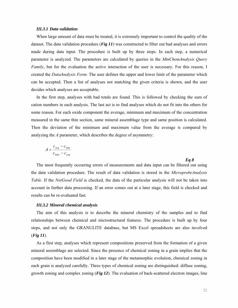
32
III.3.1 Data validation
When large amount of data must be treated, it is extremely important to control the quality of the
dataset. The data validation procedure (Fig 11) was constructed to filter out bad analyses and errors
made during data input. The procedure is built up by three steps. In each step, a numerical
parameter is analyzed. The parameters are calculated by queries in the MinChemAnalysis Query
Family, but for the evaluation the active interaction of the user is necessary. For this reason, I
created the DataAnalysis Form. The user defines the upper and lower limit of the parameter which
can be accepted. Then a list of analyses not matching the given criteria is shown, and the user
decides which analyses are acceptable.
In the first step, analyses with bad totals are found. This is followed by checking the sum of
cation numbers in each analysis. The last act is to find analyses which do not fit into the others for
some reason. For each oxide component the average, minimum and maximum of the concentration
measured in the same thin section, same mineral assemblage type and same position is calculated.
Then the deviation of the minimum and maximum value from the average is compared by
analyzing the A parameter, which describes the degree of asymmetry:
avg
avg
cccc
A−
−=
max
min
Eq 8 The most frequently occurring errors of measurements and data input can be filtered out using
the data validation procedure. The result of data validation is stored in the MicroprobeAnalysis
Table. If the NotGood Field is checked, the data of the particular analysis will not be taken into
account in further data processing. If an error comes out at a later stage, this field is checked and
results can be re-evaluated fast.
III.3.2 Mineral chemical analysis
The aim of this analysis is to describe the mineral chemistry of the samples and to find
relationships between chemical and microstructural features. The procedure is built up by four
steps, and not only the GRANULITE database, but MS Excel spreadsheets are also involved
(Fig 11).
As a first step, analyses which represent compositions preserved from the formation of a given
mineral assemblage are selected. Since the presence of chemical zoning in a grain implies that the
composition have been modified in a later stage of the metamorphic evolution, chemical zoning in
each grain is analyzed carefully. Three types of chemical zoning are distinguished: diffuse zoning,
growth zoning and complex zoning (Fig 12). The evaluation of back-scattered electron images, line
33
analysis and element distribution maps are combined with the numerical zonation analysis in the
GRANULITE database in order to determine the zoning type of each grain.
Fig 12 Spatial distribution of a component in grains with different chemical zoning patterns. Red and yellow represents the highest and lowest concentrations, respectively. a) Diffuse zoning: the composition of a phase is a continuous function of radial distance from the grain boundary. b) Growth zoning: the composition is a jump function of radial distance, and the jump is observed at a grain boundary. c) Complex zoning: superposition of diffuse and growth zoning or of different processes resulting in chemical zoning.
During the numerical zonation analysis quantitative point analyses from different positions
within the grain are compared, if they are available. For this purpose the average cation number for
all components of the grain is calculated for core ( corec ), rim ( rimc ) and zone ( zonec ) positions. The
deviation of rim and zone concentrations from the core is described by Z and Z2 parameters (Eq 9
and Eq 10), respectively. Similarly to data validation, the user sets the acceptable limits for the
parameters, then the MinChemZoning Queries filter for analyses not fitting the criteria and the user
decides which type of zonation is present. If the results are questionable, new line analyses or
element distribution maps should be made for checking.
core
corerim
ccc
Z−
=
Eq 9
core
corezone
ccc
Z−
=2
Eq 10
34
Quantitative point analyses from a grain can be further treated in two ways depending on the
zonation type of the grain. If the composition of a grain is a continuous function of the radial
distance from the grain boundary (i.e. diffuse or complex zoning is observed), individual
quantitative point analyses are taken into account in the detailed study of incomplete mineral
reactions (e.g. Section VII). In the other case, if the composition of a grain is independent from the
radial distance from the grain boundary within an interval (i.e. the grain is homogeneous or only
growth zoning is present), analyses within this interval can be averaged. In case of a homogeneous
grain, an average grain composition is created this way. If growth zoning is present, average grain
and average zone compositions are calculated. At the end of zoning analysis, the averaging
possibility for each point analysis is stored in the AvgPos Field of the MicroprobeAnalysis Table.
Average compositions from the relevant analyses can then be calculated in a few seconds by the
GRANULITE database.
Average compositions are used to test the chemical homogeneity of petrographically
distinguished mineral assemblages on different scales. This process is done by the MinChemHom
Queries. In the first step, grains from the same mineral assemblage in the same xenolith zone are
selected. The standard deviation of cation numbers for each element in each mineral within this
group is calculated using the average grain compositions. Then xenolith zones, where the standard
deviation exceeds a limit set by the user are filtered out. Point analyses from these zones are listed
for the user who decides whether the grains in the given xenolith zone are uniform in composition
or not. If inhomogeneity is found, the result is stored in the XenolithZone_Inhomogeneity Table.
The average composition of grains from xenolith zones found homogeneous is further analyzed in
the second step. Here the homogeneity of a mineral assemblage within a xenolith is studied in the
same way as it was described in the first step. The results are stored in the Xenolith_Inhomogeneity
Table.
The analysis of chemical heterogeneities on different scales is followed by the comparison of
groups identified on the basis of petrography and mineral chemistry. For this purpose, all grouping
possibilities stored in the database are put together with the results of microprobe analyses,
calculated cation numbers and other mineral chemical quantities. This is done by the
MinChemMaster queries for each mineral type. Then the query results are exported to MS Excel
worksheets, where further calculations (e.g. cation distribution on the basis of stoichiometry or end
member mole fraction calculation from these data) and basic mineral chemical plots are done.
Using the Autofilter function of Excel, it is easy to filter calculation results and plots according to
the petrographical information related to the analyses. This way petrographical and mineral
35
chemical groups can be easily associated. For comparative mineral chemical plots usually average
compositions are used.
The last step of mineral chemical analysis is a feedback to the GRANULITE database. This
includes two main actions in this case. If errors were found in the stored data or some petrographic
observations were re-evaluated on the basis of mineral chemistry, stored data are corrected. If the
combination of petrography and mineral chemistry shows new aspects of data classification, the
database structure is modified in order to host the new grouping options. Then stored data are
classified regarding the new grouping options. The feedback is extremely important to build a
progressively improving database. Examples for the feedback are shown in Section IV.2.
III.3.3 Geothermobarometric analysis
The GRANULITE database was constructed to optimize and fasten geothermobarometric
calculations and the comparison of results on large datasets. Although several programmes exist,
which calculate and compare the results of different thermometers and barometers (e.g. PTMAFIC,
SOTO and SOTO 1995), they are not applicable for large datasets. Only data from a few local
mineral assemblages can be treated simultaneously and the output is not optimized for comparison
between different assemblages. This problem can be solved by using MS Excel spreadsheets (e.g.
GPT for metapelitic rocks, RECHE and MARTINEZ 1996) for geothermobarometric estimations, but
this calculation platform has two main disadvantages. The number and order of columns is
predefined and analyses from grains which are in equilibrium with each other should be sorted by
hand. The first requires time consuming rearrangement of columns before calculation. In addition,
the list of elements treated in the calculation cannot be modified easily. The second problem is
more serious. Data should be stored in several copies, and extension of a mineral assemblage (e.g.
associating a garnet–clinopyroxene mineral pair with analyses from plagioclase grains in
equilibrium) in order to apply new methods on a large dataset can last extremely long. The
GRANULITE database offers a solution for all difficulties described above. The data structure
assures that matching analyses from all types of mineral assemblages can be found fast by writing
the appropriate query. To make the programme user-friendly, I created the GTB Forms and
Queries, which lead the user through the procedure of geothermobarometric analysis (Fig 11).
In the first step, the user chooses the mineral assemblage (e.g. Grt–Cpx or Grt–Cpx–Pl–Qtz, also
referred to as mineral ‘pair’) for which geothermobarometry should be done. By pressing the button
of the mineral assemblage, several queries run automatically. The GTB01 Queries find all local
mineral assemblages which contain the given minerals. The results are used by the GTB02 Queries
which look for all combination of grains which represent the given mineral assemblage in
36
equilibrium. In addition, these queries also associate mineral chemical data necessary for the
geothermobarometric estimation and descriptive information with the selected grains. Only
analyses made at the same lab are paired. The query results are exported to MS Excel spreadsheets.
For each mineral assemblage studied in the PhD thesis one MS Excel workbook (later referred
to as GTB workbook) summarizes several geothermobarometric methods and calibrations
established for granulite facies. The exported query results should be inserted in the Input
worksheet of the given GTB workbook. The order of fields in the query match exactly the order of
columns in the workbook. After the insertion of data, cations are redistributed as it is required by
the selected methods and pressure and/or temperature is estimated. In addition, different charts are
also included to compare graphically equilibrium constants (KD) calculated for the given mineral
‘pair’ and theoretical KD values calculated for different temperatures if the formula of the
thermometer makes it possible. This can help in the identification of true equilibrium mineral
assemblages. Further details are found in Section V.3. Since descriptive information is associated to
all numerical dataset, the AutoFilter option of Excel can be used for the interpretation of the results
in the same way as it was described in the mineral chemical analysis.
Data interpretation in MS Excel is followed by feedback to the database. The estimated P or T
values together with the results of equilibrium tests are imported to the GTBRes Tables of the
database. Further data evaluation is also possible within the database. Most frequently the average
and standard deviation of pressure and temperature estimated from different mineral assemblages
of the same mineral assemblage type from the same xenolith is calculated in order to determine the
equilibration conditions. The results are stored in the Xenolith Table, and they can be used for the
classification of the xenoliths and the construction of geotherms.
III.4 The Deep Lithosphere DataBase
Although the GRANULITE database was designed for the aims of this thesis, it is easy to
implement for other datasets where investigation methods are similar. Using the data structure of
the GRANULITE database, people may create a database for their own use much easier than
starting from the beginning. As a consequence of the block structure, complete blocks containing
tables and related database objects (queries, forms and macros) can be copied to the new database
and the block can function without making big changes. The first implementation of the
GRANULITE database was the construction of the Deep Lithosphere DataBase (DLDB).
I found it extremely important to put together and treat in a uniform way the data from the entire
lithospheric column beneath the BBHVF in order to investigate lithosphere evolution of the region.
For this reason, I tried to extend the GRANULITE database to upper mantle xenoliths from the
37
BBHVF. It was an important aim to make the new database easily accessible and open for all users
working on this topic. For this reason, I decided to make this programme accessible via internet.
Since the investigation methods are similar in case of lower crustal and upper mantle rocks
independent from appearing as xenoliths or in uplifted terrains, such a new database may be used
for samples from all over the world.
The Deep Lithosphere DataBase was designed to host these requirements. It was programmed in
postgreSQL combined with php by Mr. András Helgert. I developed the data structure and query
design. The DLDB may be regarded as a simplified version of the GRANULITE database. It has
very similar block structure as the GRANULITE database, just at the moment only the Sample and
Point Analysis Blocks are incorporated. Built-in calculations and geothermobarometric applications
run in the same system as in the GRANULITE database. The DLDB is published on the internet
(http://lrg-dldb.elte.hu). Data input to the DLDB is open for all registered authors who have
published data from deep lithospheric rocks, which may assure dynamic development of the
dataset. The amount of data uploaded by a user is unrestricted, so the database can be used for
publishing complete datasets, not only representative analyses. In addition, the dataset can be
updated any time. Besides the DLDB, all related tools necessary for making comparisons of
mineral chemical data or the results of geothermobarometry are available at the homepage. These
tools and the uploaded data are accessible to everyone. Hopefully in the future the Deep
Lithosphere DataBase may serve as a platform for comparing mineral chemistry and
geothermobarometry in deep lithospheric rocks from all over the world.
Further description of the Deep Lithospere DataBase is beyond the scope of the thesis. Interested
readers should refer to the homepage or DÉGI (2008).
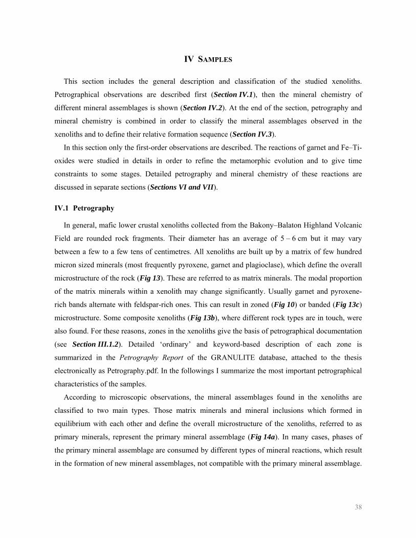
38
IV SAMPLES
This section includes the general description and classification of the studied xenoliths.
Petrographical observations are described first (Section IV.1), then the mineral chemistry of
different mineral assemblages is shown (Section IV.2). At the end of the section, petrography and
mineral chemistry is combined in order to classify the mineral assemblages observed in the
xenoliths and to define their relative formation sequence (Section IV.3).
In this section only the first-order observations are described. The reactions of garnet and Fe–Ti-
oxides were studied in details in order to refine the metamorphic evolution and to give time
constraints to some stages. Detailed petrography and mineral chemistry of these reactions are
discussed in separate sections (Sections VI and VII).
IV.1 Petrography
In general, mafic lower crustal xenoliths collected from the Bakony–Balaton Highland Volcanic
Field are rounded rock fragments. Their diameter has an average of 5 – 6 cm but it may vary
between a few to a few tens of centimetres. All xenoliths are built up by a matrix of few hundred
micron sized minerals (most frequently pyroxene, garnet and plagioclase), which define the overall
microstructure of the rock (Fig 13). These are referred to as matrix minerals. The modal proportion
of the matrix minerals within a xenolith may change significantly. Usually garnet and pyroxene-
rich bands alternate with feldspar-rich ones. This can result in zoned (Fig 10) or banded (Fig 13c)
microstructure. Some composite xenoliths (Fig 13b), where different rock types are in touch, were
also found. For these reasons, zones in the xenoliths give the basis of petrographical documentation
(see Section III.1.2). Detailed ‘ordinary’ and keyword-based description of each zone is
summarized in the Petrography Report of the GRANULITE database, attached to the thesis
electronically as Petrography.pdf. In the followings I summarize the most important petrographical
characteristics of the samples.
According to microscopic observations, the mineral assemblages found in the xenoliths are
classified to two main types. Those matrix minerals and mineral inclusions which formed in
equilibrium with each other and define the overall microstructure of the xenoliths, referred to as
primary minerals, represent the primary mineral assemblage (Fig 14a). In many cases, phases of
the primary mineral assemblage are consumed by different types of mineral reactions, which result
in the formation of new mineral assemblages, not compatible with the primary mineral assemblage.
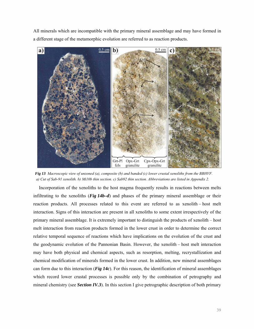
39
All minerals which are incompatible with the primary mineral assemblage and may have formed in
a different stage of the metamorphic evolution are referred to as reaction products.
Fig 13 Macroscopic view of unzoned (a), composite (b) and banded (c) lower crustal xenoliths from the BBHVF. a) Cut of Sab-91 xenolith. b) Mi10b thin section. c) Sab92 thin section. Abbreviations are listed in Appendix 2.
Incorporation of the xenoliths to the host magma frequently results in reactions between melts
infiltrating to the xenoliths (Fig 14b–d) and phases of the primary mineral assemblage or their
reaction products. All processes related to this event are referred to as xenolith – host melt
interaction. Signs of this interaction are present in all xenoliths to some extent irrespectively of the
primary mineral assemblage. It is extremely important to distinguish the products of xenolith – host
melt interaction from reaction products formed in the lower crust in order to determine the correct
relative temporal sequence of reactions which have implications on the evolution of the crust and
the geodynamic evolution of the Pannonian Basin. However, the xenolith – host melt interaction
may have both physical and chemical aspects, such as resorption, melting, recrystallization and
chemical modification of minerals formed in the lower crust. In addition, new mineral assemblages
can form due to this interaction (Fig 14c). For this reason, the identification of mineral assemblages
which record lower crustal processes is possible only by the combination of petrography and
mineral chemistry (see Section IV.3). In this section I give petrographic description of both primary
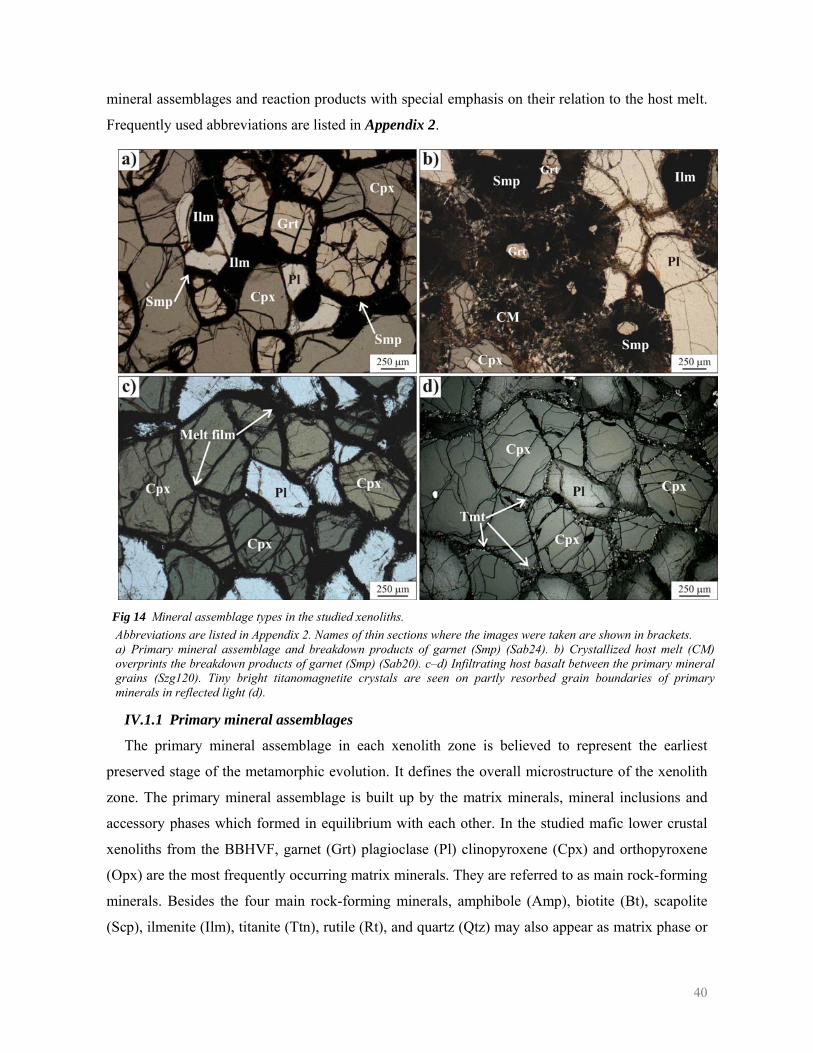
40
mineral assemblages and reaction products with special emphasis on their relation to the host melt.
Frequently used abbreviations are listed in Appendix 2.
Fig 14 Mineral assemblage types in the studied xenoliths. Abbreviations are listed in Appendix 2. Names of thin sections where the images were taken are shown in brackets. a) Primary mineral assemblage and breakdown products of garnet (Smp) (Sab24). b) Crystallized host melt (CM) overprints the breakdown products of garnet (Smp) (Sab20). c–d) Infiltrating host basalt between the primary mineral grains (Szg120). Tiny bright titanomagnetite crystals are seen on partly resorbed grain boundaries of primary minerals in reflected light (d).
IV.1.1 Primary mineral assemblages
The primary mineral assemblage in each xenolith zone is believed to represent the earliest
preserved stage of the metamorphic evolution. It defines the overall microstructure of the xenolith
zone. The primary mineral assemblage is built up by the matrix minerals, mineral inclusions and
accessory phases which formed in equilibrium with each other. In the studied mafic lower crustal
xenoliths from the BBHVF, garnet (Grt) plagioclase (Pl) clinopyroxene (Cpx) and orthopyroxene
(Opx) are the most frequently occurring matrix minerals. They are referred to as main rock-forming
minerals. Besides the four main rock-forming minerals, amphibole (Amp), biotite (Bt), scapolite
(Scp), ilmenite (Ilm), titanite (Ttn), rutile (Rt), and quartz (Qtz) may also appear as matrix phase or
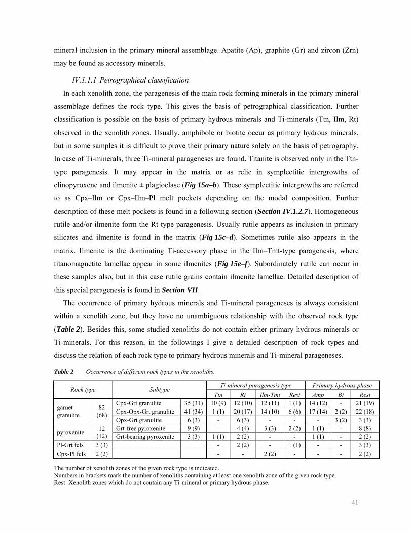
41
mineral inclusion in the primary mineral assemblage. Apatite (Ap), graphite (Gr) and zircon (Zrn)
may be found as accessory minerals.
IV.1.1.1 Petrographical classification
In each xenolith zone, the paragenesis of the main rock forming minerals in the primary mineral
assemblage defines the rock type. This gives the basis of petrographical classification. Further
classification is possible on the basis of primary hydrous minerals and Ti-minerals (Ttn, Ilm, Rt)
observed in the xenolith zones. Usually, amphibole or biotite occur as primary hydrous minerals,
but in some samples it is difficult to prove their primary nature solely on the basis of petrography.
In case of Ti-minerals, three Ti-mineral parageneses are found. Titanite is observed only in the Ttn-
type paragenesis. It may appear in the matrix or as relic in symplectitic intergrowths of
clinopyroxene and ilmenite ± plagioclase (Fig 15a–b). These symplectitic intergrowths are referred
to as Cpx–Ilm or Cpx–Ilm–Pl melt pockets depending on the modal composition. Further
description of these melt pockets is found in a following section (Section IV.1.2.7). Homogeneous
rutile and/or ilmenite form the Rt-type paragenesis. Usually rutile appears as inclusion in primary
silicates and ilmenite is found in the matrix (Fig 15c–d). Sometimes rutile also appears in the
matrix. Ilmenite is the dominating Ti-accessory phase in the Ilm–Tmt-type paragenesis, where
titanomagnetite lamellae appear in some ilmenites (Fig 15e–f). Subordinately rutile can occur in
these samples also, but in this case rutile grains contain ilmenite lamellae. Detailed description of
this special paragenesis is found in Section VII.
The occurrence of primary hydrous minerals and Ti-mineral parageneses is always consistent
within a xenolith zone, but they have no unambiguous relationship with the observed rock type
(Table 2). Besides this, some studied xenoliths do not contain either primary hydrous minerals or
Ti-minerals. For this reason, in the followings I give a detailed description of rock types and
discuss the relation of each rock type to primary hydrous minerals and Ti-mineral parageneses.
Table 2 Occurrence of different rock types in the xenoliths.
Ti-mineral paragenesis type Primary hydrous phase Rock type Subtype
Ttn Rt Ilm-Tmt Rest Amp Bt Rest Cpx-Grt granulite 35 (31) 10 (9) 12 (10) 12 (11) 1 (1) 14 (12) - 21 (19) Cpx-Opx-Grt granulite 41 (34) 1 (1) 20 (17) 14 (10) 6 (6) 17 (14) 2 (2) 22 (18) garnet
granulite 82
(68) Opx-Grt granulite 6 (3) - 6 (3) - - - 3 (2) 3 (3) Grt-free pyroxenite 9 (9) - 4 (4) 3 (3) 2 (2) 1 (1) - 8 (8) pyroxenite 12
(12) Grt-bearing pyroxenite 3 (3) 1 (1) 2 (2) - - 1 (1) - 2 (2) Pl-Grt fels 3 (3) - 2 (2) - 1 (1) - - 3 (3) Cpx-Pl fels 2 (2) - - 2 (2) - - - 2 (2)
The number of xenolith zones of the given rock type is indicated. Numbers in brackets mark the number of xenoliths containing at least one xenolith zone of the given rock type. Rest: Xenolith zones which do not contain any Ti-mineral or primary hydrous phase.
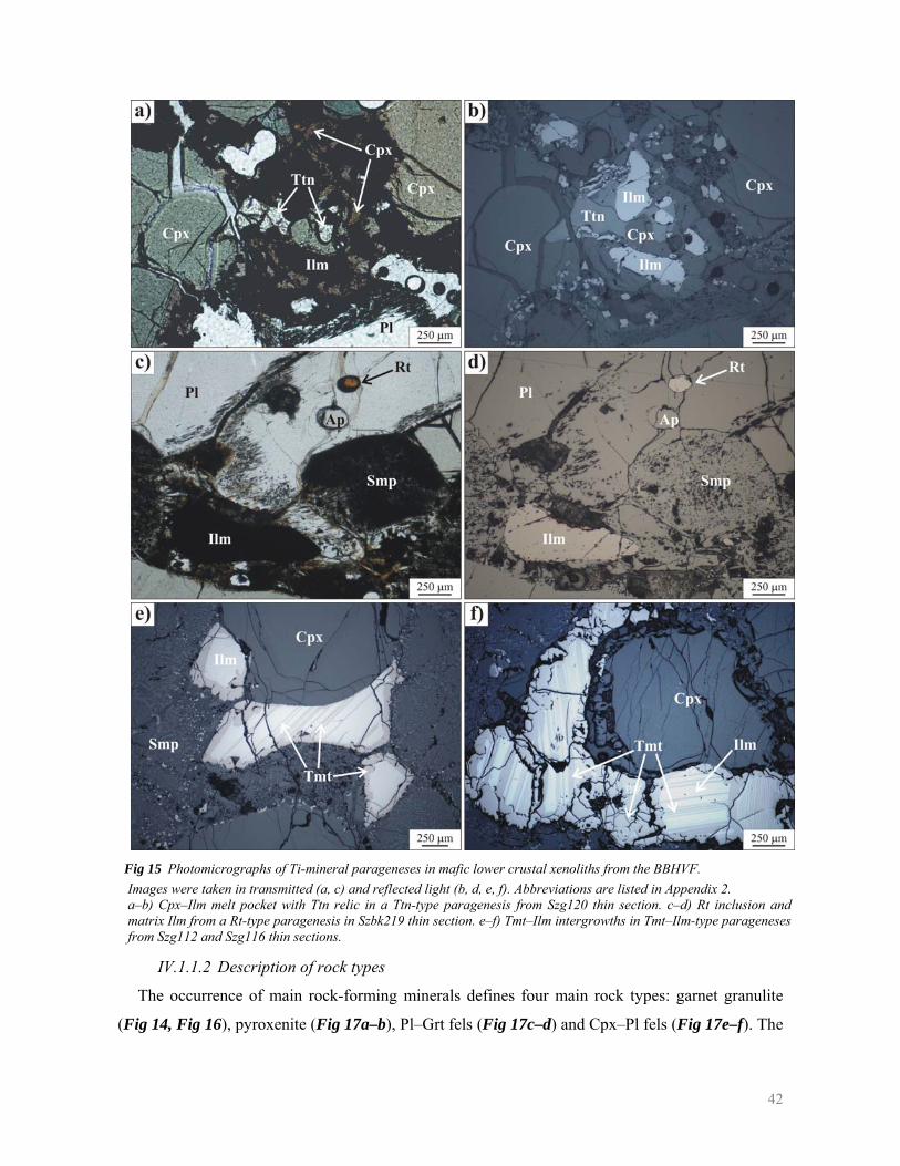
42
Fig 15 Photomicrographs of Ti-mineral parageneses in mafic lower crustal xenoliths from the BBHVF. Images were taken in transmitted (a, c) and reflected light (b, d, e, f). Abbreviations are listed in Appendix 2. a–b) Cpx–Ilm melt pocket with Ttn relic in a Ttn-type paragenesis from Szg120 thin section. c–d) Rt inclusion and matrix Ilm from a Rt-type paragenesis in Szbk219 thin section. e–f) Tmt–Ilm intergrowths in Tmt–Ilm-type parageneses from Szg112 and Szg116 thin sections.
IV.1.1.2 Description of rock types
The occurrence of main rock-forming minerals defines four main rock types: garnet granulite
(Fig 14, Fig 16), pyroxenite (Fig 17a–b), Pl–Grt fels (Fig 17c–d) and Cpx–Pl fels (Fig 17e–f). The
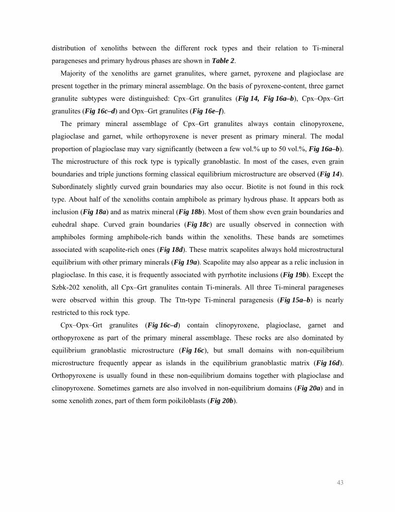
43
distribution of xenoliths between the different rock types and their relation to Ti-mineral
parageneses and primary hydrous phases are shown in Table 2.
Majority of the xenoliths are garnet granulites, where garnet, pyroxene and plagioclase are
present together in the primary mineral assemblage. On the basis of pyroxene-content, three garnet
granulite subtypes were distinguished: Cpx–Grt granulites (Fig 14, Fig 16a–b), Cpx–Opx–Grt
granulites (Fig 16c–d) and Opx–Grt granulites (Fig 16e–f).
The primary mineral assemblage of Cpx–Grt granulites always contain clinopyroxene,
plagioclase and garnet, while orthopyroxene is never present as primary mineral. The modal
proportion of plagioclase may vary significantly (between a few vol.% up to 50 vol.%, Fig 16a–b).
The microstructure of this rock type is typically granoblastic. In most of the cases, even grain
boundaries and triple junctions forming classical equilibrium microstructure are observed (Fig 14).
Subordinately slightly curved grain boundaries may also occur. Biotite is not found in this rock
type. About half of the xenoliths contain amphibole as primary hydrous phase. It appears both as
inclusion (Fig 18a) and as matrix mineral (Fig 18b). Most of them show even grain boundaries and
euhedral shape. Curved grain boundaries (Fig 18c) are usually observed in connection with
amphiboles forming amphibole-rich bands within the xenoliths. These bands are sometimes
associated with scapolite-rich ones (Fig 18d). These matrix scapolites always hold microstructural
equilibrium with other primary minerals (Fig 19a). Scapolite may also appear as a relic inclusion in
plagioclase. In this case, it is frequently associated with pyrrhotite inclusions (Fig 19b). Except the
Szbk-202 xenolith, all Cpx–Grt granulites contain Ti-minerals. All three Ti-mineral parageneses
were observed within this group. The Ttn-type Ti-mineral paragenesis (Fig 15a–b) is nearly
restricted to this rock type.
Cpx–Opx–Grt granulites (Fig 16c–d) contain clinopyroxene, plagioclase, garnet and
orthopyroxene as part of the primary mineral assemblage. These rocks are also dominated by
equilibrium granoblastic microstructure (Fig 16c), but small domains with non-equilibrium
microstructure frequently appear as islands in the equilibrium granoblastic matrix (Fig 16d).
Orthopyroxene is usually found in these non-equilibrium domains together with plagioclase and
clinopyroxene. Sometimes garnets are also involved in non-equilibrium domains (Fig 20a) and in
some xenolith zones, part of them form poikiloblasts (Fig 20b).
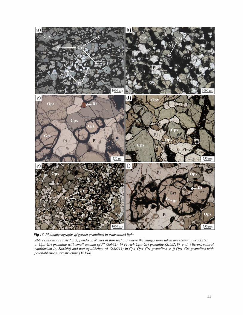
44
Fig 16 Photomicrographs of garnet granulites in transmitted light. Abbreviations are listed in Appendix 2. Names of thin sections where the images were taken are shown in brackets. a) Cpx–Grt granulite with small amount of Pl (Sab32). b) Pl-rich Cpx–Grt granulite (Szbk219). c–d) Microstructural equilibrium (c, Sab39a) and non-equilibrium (d, Szbk211) in Cpx–Opx–Grt granulites. e–f) Opx–Grt granulites with poikiloblastic microstructure (Mi19a).
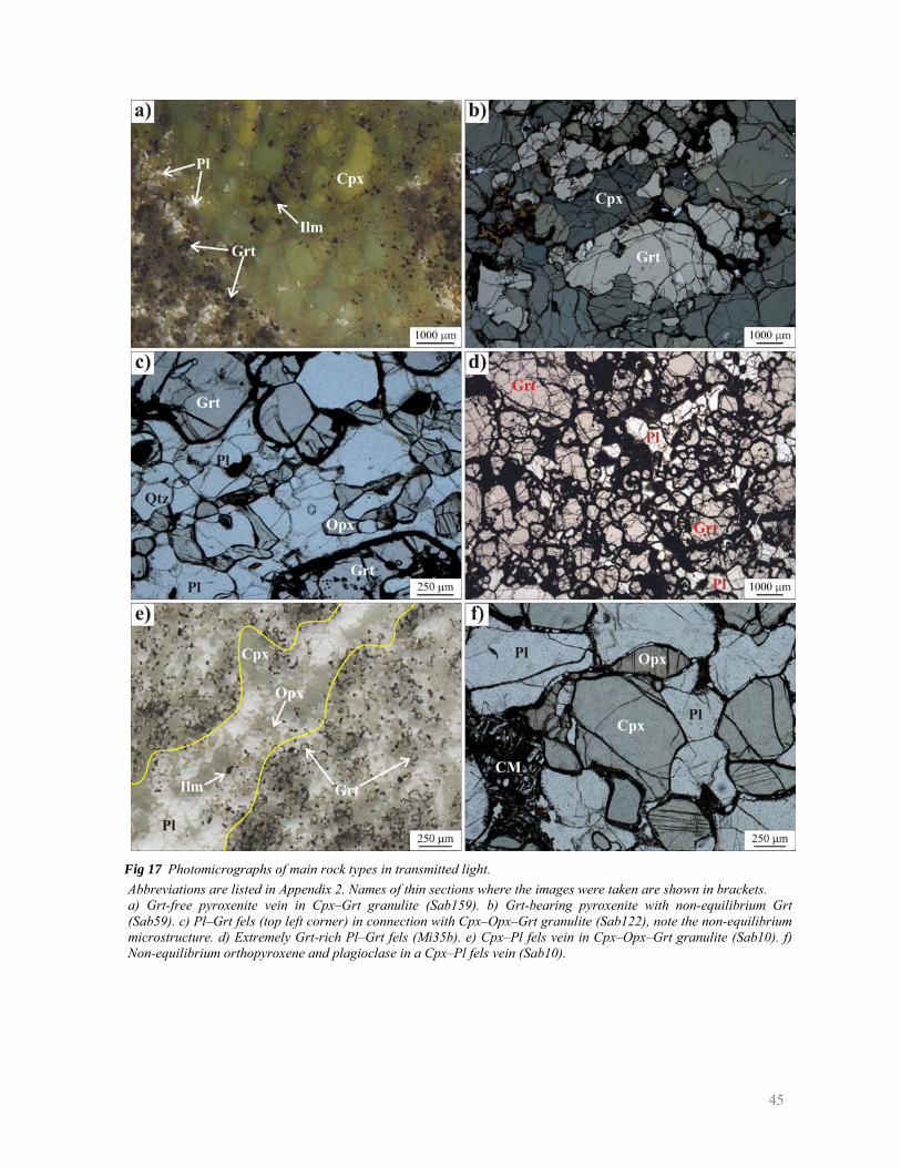
45
Fig 17 Photomicrographs of main rock types in transmitted light. Abbreviations are listed in Appendix 2. Names of thin sections where the images were taken are shown in brackets. a) Grt-free pyroxenite vein in Cpx–Grt granulite (Sab159). b) Grt-bearing pyroxenite with non-equilibrium Grt (Sab59). c) Pl–Grt fels (top left corner) in connection with Cpx–Opx–Grt granulite (Sab122), note the non-equilibrium microstructure. d) Extremely Grt-rich Pl–Grt fels (Mi35b). e) Cpx–Pl fels vein in Cpx–Opx–Grt granulite (Sab10). f) Non-equilibrium orthopyroxene and plagioclase in a Cpx–Pl fels vein (Sab10).
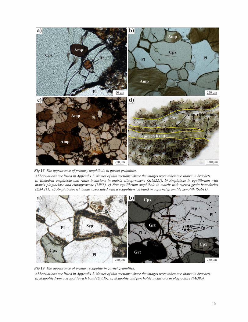
46
Fig 18 The appearance of primary amphibole in garnet granulites. Abbreviations are listed in Appendix 2. Names of thin sections where the images were taken are shown in brackets. a) Euhedral amphibole and rutile inclusions in matrix clinopyroxene (Szbk221). b) Amphibole in equilibrium with matrix plagioclase and clinopyroxene (Mi33). c) Non-equilibrium amphibole in matrix with curved grain boundaries (Szbk211). d) Amphibole-rich bands associated with a scapolite-rich band in a garnet granulite xenolith (Sab11).
Fig 19 The appearance of primary scapolite in garnet granulites. Abbreviations are listed in Appendix 2. Names of thin sections where the images were taken are shown in brackets. a) Scapolite from a scapolite-rich band (Sab19). b) Scapolite and pyrrhotite inclusions in plagioclase (Mi39a).
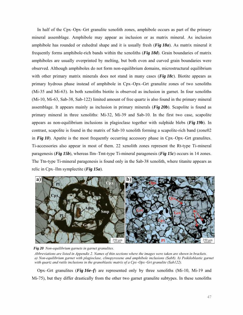
47
In half of the Cpx–Opx–Grt granulite xenolith zones, amphibole occurs as part of the primary
mineral assemblage. Amphibole may appear as inclusion or as matrix mineral. As inclusion
amphibole has rounded or euhedral shape and it is usually fresh (Fig 18a). As matrix mineral it
frequently forms amphibole-rich bands within the xenoliths (Fig 18d). Grain boundaries of matrix
amphiboles are usually overprinted by melting, but both even and curved grain boundaries were
observed. Although amphiboles do not form non-equilibrium domains, microstructural equilibrium
with other primary matrix minerals does not stand in many cases (Fig 18c). Biotite appears as
primary hydrous phase instead of amphibole in Cpx–Opx–Grt granulite zones of two xenoliths
(Mi-35 and Mi-63). In both xenoliths biotite is observed as inclusion in garnet. In four xenoliths
(Mi-10, Mi-63, Sab-38, Sab-122) limited amount of free quartz is also found in the primary mineral
assemblage. It appears mainly as inclusion in primary minerals (Fig 20b). Scapolite is found as
primary mineral in three xenoliths: Mi-32, Mi-39 and Sab-10. In the first two case, scapolite
appears as non-equilibrium inclusions in plagioclase together with sulphide blebs (Fig 19b). In
contrast, scapolite is found in the matrix of Sab-10 xenolith forming a scapolite-rich band (zone02
in Fig 10). Apatite is the most frequently occurring accessory phase in Cpx–Opx–Grt granulites.
Ti-accessories also appear in most of them. 22 xenolith zones represent the Rt-type Ti-mineral
paragenesis (Fig 15b), whereas Ilm–Tmt-type Ti-mineral paragenesis (Fig 15c) occurs in 14 zones.
The Ttn-type Ti-mineral paragenesis is found only in the Sab-38 xenolith, where titanite appears as
relic in Cpx–Ilm symplectite (Fig 15a).
Fig 20 Non-equilibrium garnets in garnet granulites. Abbreviations are listed in Appendix 2. Names of thin sections where the images were taken are shown in brackets. a) Non-equilibrium garnet with plagioclase, clinopyroxene and amphibole inclusions (Sab8). b) Poikiloblastic garnet with quartz and rutile inclusions in the granoblastic matrix of a Cpx–Opx–Grt granulite (Sab122).
Opx–Grt granulites (Fig 16e–f) are represented only by three xenoliths (Mi-10, Mi-19 and
Mi-75), but they differ drastically from the other two garnet granulite subtypes. In these xenoliths
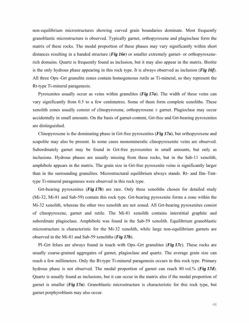
48
non-equilibrium microstructures showing curved grain boundaries dominate. Most frequently
granoblastic microstructure is observed. Typically garnet, orthopyroxene and plagioclase form the
matrix of these rocks. The modal proportion of these phases may vary significantly within short
distances resulting in a banded structure (Fig 16e) or smaller extremely garnet- or orthopyroxene-
rich domains. Quartz is frequently found as inclusion, but it may also appear in the matrix. Biotite
is the only hydrous phase appearing in this rock type. It is always observed as inclusion (Fig 16f).
All three Opx–Grt granulite zones contain homogeneous rutile as Ti-mineral, so they represent the
Rt-type Ti-mineral paragenesis.
Pyroxenites usually occur as veins within granulites (Fig 17a). The width of these veins can
vary significantly from 0.5 to a few centimetres. Some of them form complete xenoliths. These
xenolith zones usually consist of clinopyroxene, orthopyroxene ± garnet. Plagioclase may occur
accidentally in small amounts. On the basis of garnet-content, Grt-free and Grt-bearing pyroxenites
are distinguished.
Clinopyroxene is the dominating phase in Grt-free pyroxenites (Fig 17a), but orthopyroxene and
scapolite may also be present. In some cases monomineralic clinopyroxenite veins are observed.
Subordinately garnet may be found in Grt-free pyroxenites in small amounts, but only as
inclusions. Hydrous phases are usually missing from these rocks, but in the Sab-11 xenolith,
amphibole appears in the matrix. The grain size in Grt-free pyroxenite veins is significantly larger
than in the surrounding granulites. Microstructural equilibrium always stands. Rt- and Ilm–Tmt-
type Ti-mineral parageneses were observed in this rock type.
Grt-bearing pyroxenites (Fig 17b) are rare. Only three xenoliths chosen for detailed study
(Mi-32, Mi-81 and Sab-59) contain this rock type. Grt-bearing pyroxenite forms a zone within the
Mi-32 xenolith, whereas the other two xenolith are not zoned. All Grt-bearing pyroxenites consist
of clinopyroxene, garnet and rutile. The Mi-81 xenolith contains interstitial graphite and
subordinate plagioclase. Amphibole was found in the Sab-59 xenolith. Equilibrium granoblastic
microstructure is characteristic for the Mi-32 xenolith, while large non-equilibrium garnets are
observed in the Mi-81 and Sab-59 xenoliths (Fig 17b).
Pl–Grt felses are always found in touch with Opx–Grt granulites (Fig 17c). These rocks are
usually coarse-grained aggregates of garnet, plagioclase and quartz. The average grain size can
reach a few millimeters. Only the Rt-type Ti-mineral paragenesis occurs in this rock type. Primary
hydrous phase is not observed. The modal proportion of garnet can reach 80 vol.% (Fig 17d).
Quartz is usually found as inclusions, but it can occur in the matrix also if the modal proportion of
garnet is smaller (Fig 17a). Granoblastic microstructure is characteristic for this rock type, but
garnet porphyroblasts may also occur.
49
The appearance of Cpx–Pl felses is similar to the appearance of pyroxenites. Usually they form
bands within granulites (Fig 17e), but they can appear as complete xenoliths also (TÖRÖK in
preparation). The average grain size is usually slightly larger than in the surrounding granulites.
Cpx–Pl felses consist of clinopyroxene, plagioclase ± orthopyroxene. Orthopyroxene usually
occurs in non-equilibrium domains in the equilibrium granoblastic matrix (Fig 17f). Hydrous
phases do not occur in this rock type. Ilm–Tmt is the characteristic Ti-mineral paragenesis type.
IV.1.2 Reactions observed
Phases of the primary mineral assemblage show several types of mineral reactions which took
place in the late stages of metamorphic evolution. Some of the mineral reactions are related to the
xenolith – host melt interaction. However, these reaction products are usually difficult to
distinguish from the ones formed in the lower crust on the basis of petrography. In the followings,
the observed reaction types and their relation to infiltrating melts will be shown.
IV.1.2.1 Garnet breakdown
The breakdown of garnet is the most frequently occurring mineral reaction in the studied
samples. It is observed in all rock types containing garnet. For this reason, microstructure and
chemistry of the breakdown products have been investigated in details and are described in a
separate section (see Section VI). Here only the most important microstructural characteristics of
mineral assemblages formed after garnet are summarized briefly.
The breakdown products of garnet usually form a non-transparent, deep brownish or opaque
kelyphitic rim of constant thickness around the garnet relic (e.g. Fig 14a). In some cases the entire
garnet is consumed, and kelyphites form pseudomorphs (e.g. Fig 15c). In general, phases of the
kelyphites are so fine-grained that the individual minerals can only be distinguished under electron
microscope. On the basis of back-scattered electron images (Fig 21a), fine-grained kelyphites are
vermicular intergrowths of orthopyroxene, plagioclase and spinel. This mineral assemblage,
referred to as type 1 symplectite, replaces the garnet along a sharp reaction front. Usually the
reaction products are submicron-sized at the reaction front and they show coarsening towards the
former garnet grain boundary. In some cases, especially in kelyphites in connection with infiltrating
melts, the grain size in the outer portion of the reaction rim suddenly increase up to a few tens of
microns (Fig 21a).
Type 1 symplectites are observed in all xenoliths containing garnet. However, in some samples a
second mineral assemblage, referred to as type 2 symplectite, also occurs in the pseudomorphs after
garnet (Fig 21b). This assemblage always contains olivine and plagioclase, which are frequently
associated with spinel and melt patches. Type 2 symplectites occur at the outer portion of the
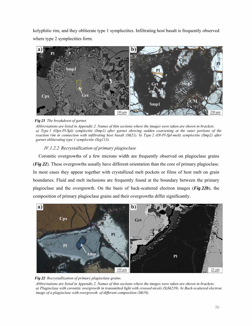
50
kelyphitic rim, and they obliterate type 1 symplectites. Infiltrating host basalt is frequently observed
where type 2 symplectites form.
Fig 21 The breakdown of garnet. Abbreviations are listed in Appendix 2. Names of thin sections where the images were taken are shown in brackets. a) Type 1 (Opx-Pl-Spl) symplectite (Smp1) after garnet showing sudden coarsening at the outer portions of the reaction rim in connection with infiltrating host basalt (Mi21). b) Type 2 (Ol-Pl-Spl-melt) symplectite (Smp2) after garnet obliterating type 1 symplectite (Szg113).
IV.1.2.2 Recrystallization of primary plagioclase
Coronitic overgrowths of a few microns width are frequently observed on plagioclase grains
(Fig 22). These overgrowths usually have different orientation than the core of primary plagioclase.
In most cases they appear together with crystallized melt pockets or films of host melt on grain
boundaries. Fluid and melt inclusions are frequently found at the boundary between the primary
plagioclase and the overgrowth. On the basis of back-scattered electron images (Fig 22b), the
composition of primary plagioclase grains and their overgrowths differ significantly.
Fig 22 Recrystallization of primary plagioclase grains. Abbreviations are listed in Appendix 2. Names of thin sections where the images were taken are shown in brackets. a) Plagioclase with coronitic overgrowth in transmitted light with crossed nicols (Szbk219). b) Back-scattered electron image of a plagioclase with overgrowth of different composition (Mi19).
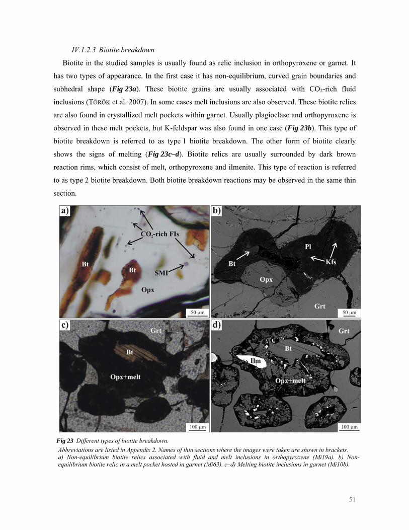
51
IV.1.2.3 Biotite breakdown
Biotite in the studied samples is usually found as relic inclusion in orthopyroxene or garnet. It
has two types of appearance. In the first case it has non-equilibrium, curved grain boundaries and
subhedral shape (Fig 23a). These biotite grains are usually associated with CO2-rich fluid
inclusions (TÖRÖK et al. 2007). In some cases melt inclusions are also observed. These biotite relics
are also found in crystallized melt pockets within garnet. Usually plagioclase and orthopyroxene is
observed in these melt pockets, but K-feldspar was also found in one case (Fig 23b). This type of
biotite breakdown is referred to as type 1 biotite breakdown. The other form of biotite clearly
shows the signs of melting (Fig 23c–d). Biotite relics are usually surrounded by dark brown
reaction rims, which consist of melt, orthopyroxene and ilmenite. This type of reaction is referred
to as type 2 biotite breakdown. Both biotite breakdown reactions may be observed in the same thin
section.
Fig 23 Different types of biotite breakdown. Abbreviations are listed in Appendix 2. Names of thin sections where the images were taken are shown in brackets. a) Non-equilibrium biotite relics associated with fluid and melt inclusions in orthopyroxene (Mi19a). b) Non-equilibrium biotite relic in a melt pocket hosted in garnet (Mi63). c–d) Melting biotite inclusions in garnet (Mi10b).
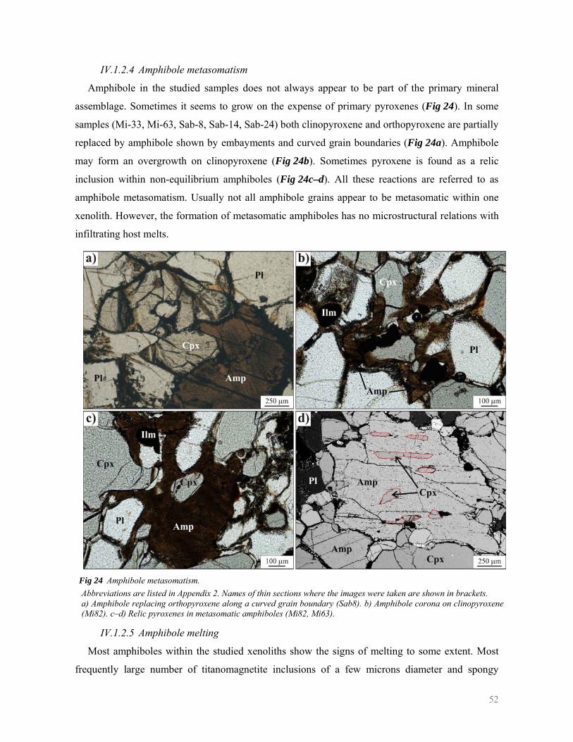
52
IV.1.2.4 Amphibole metasomatism
Amphibole in the studied samples does not always appear to be part of the primary mineral
assemblage. Sometimes it seems to grow on the expense of primary pyroxenes (Fig 24). In some
samples (Mi-33, Mi-63, Sab-8, Sab-14, Sab-24) both clinopyroxene and orthopyroxene are partially
replaced by amphibole shown by embayments and curved grain boundaries (Fig 24a). Amphibole
may form an overgrowth on clinopyroxene (Fig 24b). Sometimes pyroxene is found as a relic
inclusion within non-equilibrium amphiboles (Fig 24c–d). All these reactions are referred to as
amphibole metasomatism. Usually not all amphibole grains appear to be metasomatic within one
xenolith. However, the formation of metasomatic amphiboles has no microstructural relations with
infiltrating host melts.
Fig 24 Amphibole metasomatism. Abbreviations are listed in Appendix 2. Names of thin sections where the images were taken are shown in brackets. a) Amphibole replacing orthopyroxene along a curved grain boundary (Sab8). b) Amphibole corona on clinopyroxene (Mi82). c–d) Relic pyroxenes in metasomatic amphiboles (Mi82, Mi63).
IV.1.2.5 Amphibole melting
Most amphiboles within the studied xenoliths show the signs of melting to some extent. Most
frequently large number of titanomagnetite inclusions of a few microns diameter and spongy
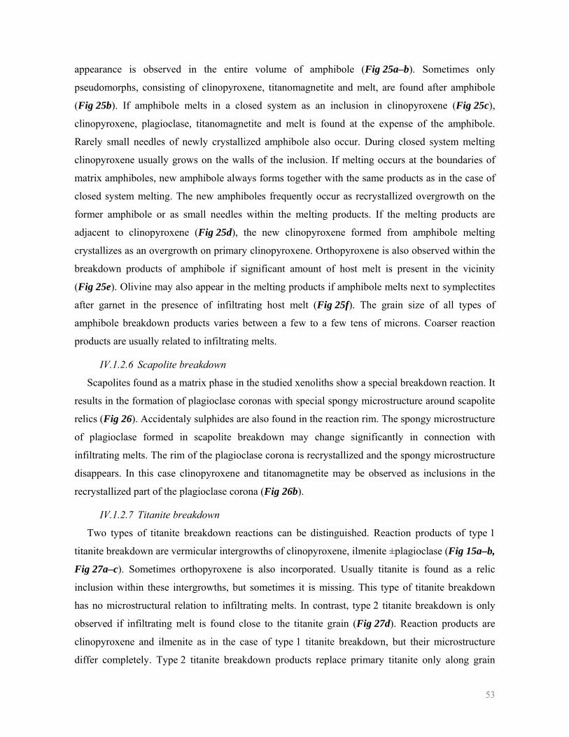
53
appearance is observed in the entire volume of amphibole (Fig 25a–b). Sometimes only
pseudomorphs, consisting of clinopyroxene, titanomagnetite and melt, are found after amphibole
(Fig 25b). If amphibole melts in a closed system as an inclusion in clinopyroxene (Fig 25c),
clinopyroxene, plagioclase, titanomagnetite and melt is found at the expense of the amphibole.
Rarely small needles of newly crystallized amphibole also occur. During closed system melting
clinopyroxene usually grows on the walls of the inclusion. If melting occurs at the boundaries of
matrix amphiboles, new amphibole always forms together with the same products as in the case of
closed system melting. The new amphiboles frequently occur as recrystallized overgrowth on the
former amphibole or as small needles within the melting products. If the melting products are
adjacent to clinopyroxene (Fig 25d), the new clinopyroxene formed from amphibole melting
crystallizes as an overgrowth on primary clinopyroxene. Orthopyroxene is also observed within the
breakdown products of amphibole if significant amount of host melt is present in the vicinity
(Fig 25e). Olivine may also appear in the melting products if amphibole melts next to symplectites
after garnet in the presence of infiltrating host melt (Fig 25f). The grain size of all types of
amphibole breakdown products varies between a few to a few tens of microns. Coarser reaction
products are usually related to infiltrating melts.
IV.1.2.6 Scapolite breakdown
Scapolites found as a matrix phase in the studied xenoliths show a special breakdown reaction. It
results in the formation of plagioclase coronas with special spongy microstructure around scapolite
relics (Fig 26). Accidentaly sulphides are also found in the reaction rim. The spongy microstructure
of plagioclase formed in scapolite breakdown may change significantly in connection with
infiltrating melts. The rim of the plagioclase corona is recrystallized and the spongy microstructure
disappears. In this case clinopyroxene and titanomagnetite may be observed as inclusions in the
recrystallized part of the plagioclase corona (Fig 26b).
IV.1.2.7 Titanite breakdown
Two types of titanite breakdown reactions can be distinguished. Reaction products of type 1
titanite breakdown are vermicular intergrowths of clinopyroxene, ilmenite ±plagioclase (Fig 15a–b,
Fig 27a–c). Sometimes orthopyroxene is also incorporated. Usually titanite is found as a relic
inclusion within these intergrowths, but sometimes it is missing. This type of titanite breakdown
has no microstructural relation to infiltrating melts. In contrast, type 2 titanite breakdown is only
observed if infiltrating melt is found close to the titanite grain (Fig 27d). Reaction products are
clinopyroxene and ilmenite as in the case of type 1 titanite breakdown, but their microstructure
differ completely. Type 2 titanite breakdown products replace primary titanite only along grain
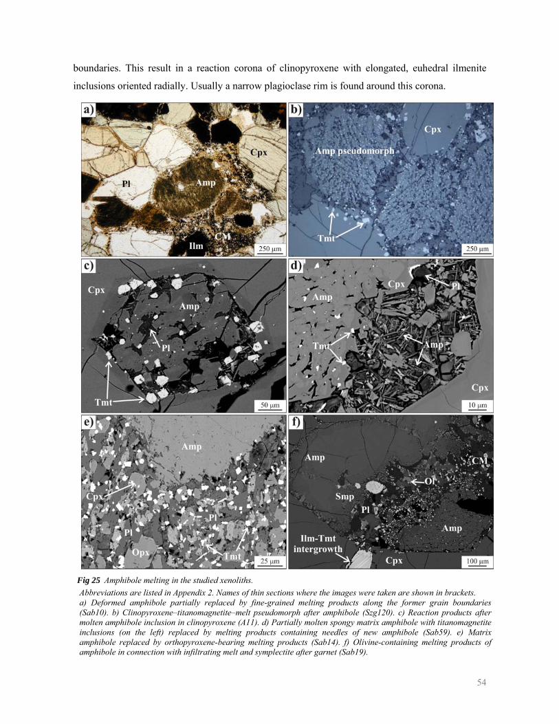
54
boundaries. This result in a reaction corona of clinopyroxene with elongated, euhedral ilmenite
inclusions oriented radially. Usually a narrow plagioclase rim is found around this corona.
Fig 25 Amphibole melting in the studied xenoliths. Abbreviations are listed in Appendix 2. Names of thin sections where the images were taken are shown in brackets. a) Deformed amphibole partially replaced by fine-grained melting products along the former grain boundaries (Sab10). b) Clinopyroxene–titanomagnetite–melt pseudomorph after amphibole (Szg120). c) Reaction products after molten amphibole inclusion in clinopyroxene (A11). d) Partially molten spongy matrix amphibole with titanomagnetite inclusions (on the left) replaced by melting products containing needles of new amphibole (Sab59). e) Matrix amphibole replaced by orthopyroxene-bearing melting products (Sab14). f) Olivine-containing melting products of amphibole in connection with infiltrating melt and symplectite after garnet (Sab19).
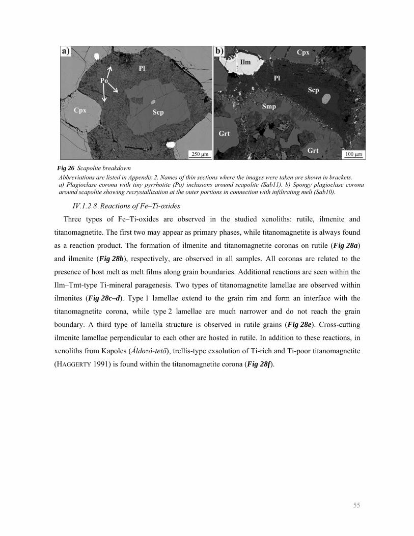
55
Fig 26 Scapolite breakdown Abbreviations are listed in Appendix 2. Names of thin sections where the images were taken are shown in brackets. a) Plagioclase corona with tiny pyrrhotite (Po) inclusions around scapolite (Sab11). b) Spongy plagioclase corona around scapolite showing recrystallization at the outer portions in connection with infiltrating melt (Sab10).
IV.1.2.8 Reactions of Fe–Ti-oxides
Three types of Fe–Ti-oxides are observed in the studied xenoliths: rutile, ilmenite and
titanomagnetite. The first two may appear as primary phases, while titanomagnetite is always found
as a reaction product. The formation of ilmenite and titanomagnetite coronas on rutile (Fig 28a)
and ilmenite (Fig 28b), respectively, are observed in all samples. All coronas are related to the
presence of host melt as melt films along grain boundaries. Additional reactions are seen within the
Ilm–Tmt-type Ti-mineral paragenesis. Two types of titanomagnetite lamellae are observed within
ilmenites (Fig 28c–d). Type 1 lamellae extend to the grain rim and form an interface with the
titanomagnetite corona, while type 2 lamellae are much narrower and do not reach the grain
boundary. A third type of lamella structure is observed in rutile grains (Fig 28e). Cross-cutting
ilmenite lamellae perpendicular to each other are hosted in rutile. In addition to these reactions, in
xenoliths from Kapolcs (Áldozó-tető), trellis-type exsolution of Ti-rich and Ti-poor titanomagnetite
(HAGGERTY 1991) is found within the titanomagnetite corona (Fig 28f).
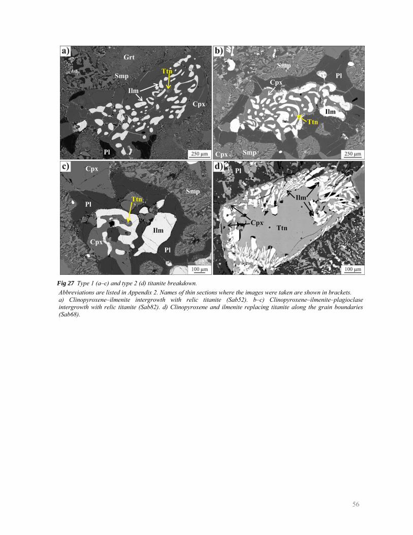
56
Fig 27 Type 1 (a–c) and type 2 (d) titanite breakdown. Abbreviations are listed in Appendix 2. Names of thin sections where the images were taken are shown in brackets. a) Clinopyroxene–ilmenite intergrowth with relic titanite (Sab52). b–c) Clinopyroxene–ilmenite–plagioclase intergrowth with relic titanite (Sab82). d) Clinopyroxene and ilmenite replacing titanite along the grain boundaries (Sab68).
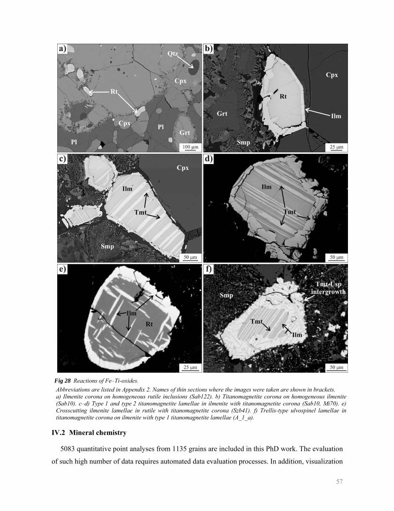
57
Fig 28 Reactions of Fe–Ti-oxides. Abbreviations are listed in Appendix 2. Names of thin sections where the images were taken are shown in brackets. a) Ilmenite corona on homogeneous rutile inclusions (Sab122). b) Titanomagnetite corona on homogeneous ilmenite (Sab10). c–d) Type 1 and type 2 titanomagnetite lamellae in ilmenite with titanomagnetite corona (Sab10, Mi70). e) Crosscutting ilmenite lamellae in rutile with titanomagnetite corona (Szb41). f) Trellis-type ulvospinel lamellae in titanomagnetite corona on ilmenite with type 1 titanomagnetite lamellae (A_1_a).
IV.2 Mineral chemistry
5083 quantitative point analyses from 1135 grains are included in this PhD work. The evaluation
of such high number of data requires automated data evaluation processes. In addition, visualization
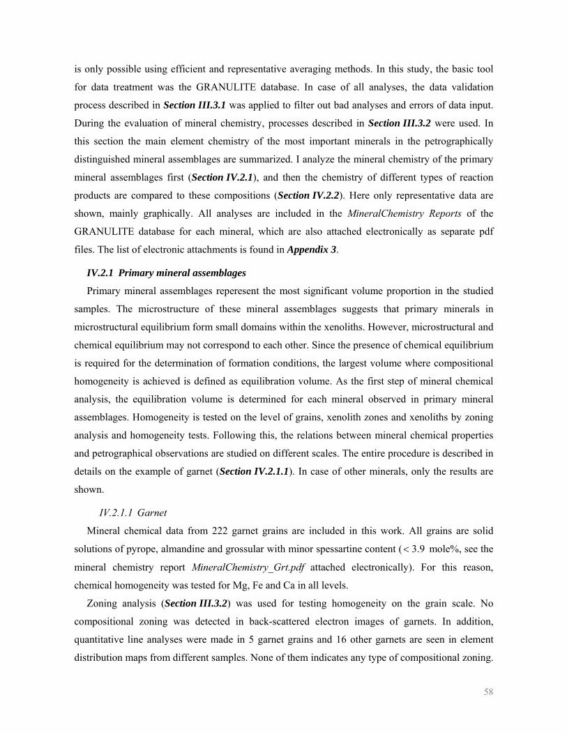
58
is only possible using efficient and representative averaging methods. In this study, the basic tool
for data treatment was the GRANULITE database. In case of all analyses, the data validation
process described in Section III.3.1 was applied to filter out bad analyses and errors of data input.
During the evaluation of mineral chemistry, processes described in Section III.3.2 were used. In
this section the main element chemistry of the most important minerals in the petrographically
distinguished mineral assemblages are summarized. I analyze the mineral chemistry of the primary
mineral assemblages first (Section IV.2.1), and then the chemistry of different types of reaction
products are compared to these compositions (Section IV.2.2). Here only representative data are
shown, mainly graphically. All analyses are included in the MineralChemistry Reports of the
GRANULITE database for each mineral, which are also attached electronically as separate pdf
files. The list of electronic attachments is found in Appendix 3.
IV.2.1 Primary mineral assemblages
Primary mineral assemblages reperesent the most significant volume proportion in the studied
samples. The microstructure of these mineral assemblages suggests that primary minerals in
microstructural equilibrium form small domains within the xenoliths. However, microstructural and
chemical equilibrium may not correspond to each other. Since the presence of chemical equilibrium
is required for the determination of formation conditions, the largest volume where compositional
homogeneity is achieved is defined as equilibration volume. As the first step of mineral chemical
analysis, the equilibration volume is determined for each mineral observed in primary mineral
assemblages. Homogeneity is tested on the level of grains, xenolith zones and xenoliths by zoning
analysis and homogeneity tests. Following this, the relations between mineral chemical properties
and petrographical observations are studied on different scales. The entire procedure is described in
details on the example of garnet (Section IV.2.1.1). In case of other minerals, only the results are
shown.
IV.2.1.1 Garnet
Mineral chemical data from 222 garnet grains are included in this work. All grains are solid
solutions of pyrope, almandine and grossular with minor spessartine content ( 9.3< mole%, see the
mineral chemistry report MineralChemistry_Grt.pdf attached electronically). For this reason,
chemical homogeneity was tested for Mg, Fe and Ca in all levels.
Zoning analysis (Section III.3.2) was used for testing homogeneity on the grain scale. No
compositional zoning was detected in back-scattered electron images of garnets. In addition,
quantitative line analyses were made in 5 garnet grains and 16 other garnets are seen in element
distribution maps from different samples. None of them indicates any type of compositional zoning.
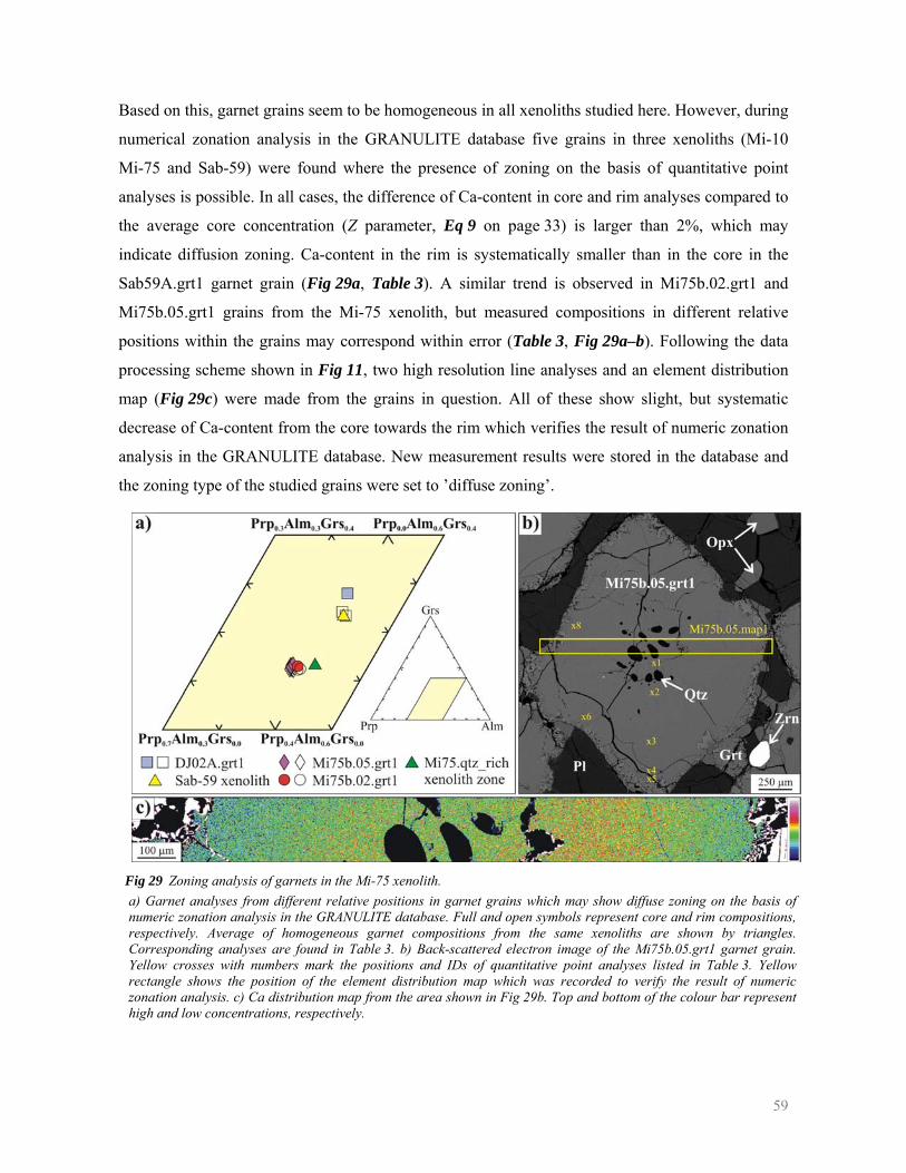
59
Based on this, garnet grains seem to be homogeneous in all xenoliths studied here. However, during
numerical zonation analysis in the GRANULITE database five grains in three xenoliths (Mi-10
Mi-75 and Sab-59) were found where the presence of zoning on the basis of quantitative point
analyses is possible. In all cases, the difference of Ca-content in core and rim analyses compared to
the average core concentration (Z parameter, Eq 9 on page 33) is larger than 2%, which may
indicate diffusion zoning. Ca-content in the rim is systematically smaller than in the core in the
Sab59A.grt1 garnet grain (Fig 29a, Table 3). A similar trend is observed in Mi75b.02.grt1 and
Mi75b.05.grt1 grains from the Mi-75 xenolith, but measured compositions in different relative
positions within the grains may correspond within error (Table 3, Fig 29a–b). Following the data
processing scheme shown in Fig 11, two high resolution line analyses and an element distribution
map (Fig 29c) were made from the grains in question. All of these show slight, but systematic
decrease of Ca-content from the core towards the rim which verifies the result of numeric zonation
analysis in the GRANULITE database. New measurement results were stored in the database and
the zoning type of the studied grains were set to ’diffuse zoning’.
Fig 29 Zoning analysis of garnets in the Mi-75 xenolith. a) Garnet analyses from different relative positions in garnet grains which may show diffuse zoning on the basis of numeric zonation analysis in the GRANULITE database. Full and open symbols represent core and rim compositions, respectively. Average of homogeneous garnet compositions from the same xenoliths are shown by triangles. Corresponding analyses are found in Table 3. b) Back-scattered electron image of the Mi75b.05.grt1 garnet grain. Yellow crosses with numbers mark the positions and IDs of quantitative point analyses listed in Table 3. Yellow rectangle shows the position of the element distribution map which was recorded to verify the result of numeric zonation analysis. c) Ca distribution map from the area shown in Fig 29b. Top and bottom of the colour bar represent high and low concentrations, respectively.
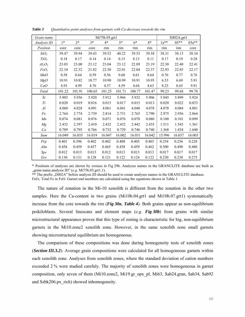
60
Table 3 Quantitative point analyses from garnets with Ca-decrease towards the rim
Grain name Mi75b.05.grt1 DJ02A.grt1 Analysis ID 1* 2* 3* 4* 5* 6* 8* 1a** 05** 03a**
Position core core core rim rim rim rim rim rim core SiO2 39.47 39.94 39.43 39.52 40.22 39.53 39.58 38.31 38.13 38.34 TiO2 0.18 0.17 0.14 0.14 0.15 0.13 0.11 0.17 0.19 0.28 Al2O3 23.03 23.00 23.12 23.04 23.12 22.89 23.19 22.30 22.40 22.41 FeOt 22.10 22.32 21.82 22.50 22.01 22.04 22.37 22.93 22.85 22.17 MnO 0.58 0.64 0.59 0.56 0.60 0.61 0.64 0.76 0.77 0.76 MgO 10.91 10.82 10.77 10.90 10.99 10.91 10.95 6.53 6.69 5.91 CaO 4.93 4.99 4.76 4.57 4.59 4.64 4.63 8.23 8.65 9.91 Total 101.22 101.91 100.65 101.25 101.71 100.77 101.47 99.23 99.68 99.78
Si 5.903 5.936 5.920 5.912 5.966 5.932 5.906 5.945 5.899 5.924 Ti 0.020 0.019 0.016 0.015 0.017 0.015 0.013 0.020 0.022 0.033 Al 4.060 4.028 4.091 4.061 4.041 4.048 4.078 4.078 4.084 4.081 Fe 2.764 2.774 2.739 2.814 2.731 2.765 2.790 2.975 2.956 2.864 Mn 0.074 0.081 0.076 0.071 0.076 0.078 0.080 0.100 0.101 0.099 Mg 2.432 2.397 2.410 2.432 2.432 2.442 2.435 1.511 1.543 1.361 Ca 0.789 0.795 0.766 0.732 0.729 0.746 0.740 1.368 1.434 1.640
Sum 16.049 16.035 16.019 16.047 16.002 16.031 16.042 15.996 16.037 16.003Prp 0.401 0.396 0.402 0.402 0.408 0.405 0.403 0.254 0.256 0.228 Alm 0.456 0.459 0.457 0.465 0.458 0.459 0.462 0.500 0.490 0.480 Sps 0.012 0.013 0.013 0.012 0.013 0.013 0.013 0.017 0.017 0.017 Grs 0.130 0.131 0.128 0.121 0.122 0.124 0.122 0.230 0.238 0.275
* Positions of analyses are shown by crosses in Fig 29b. Analyses names in the GRANULITE database are built as „grain name.analysis ID” (e.g. Mi75b.05.grt1.1). ** The prefix „DJ02A” before analysis ID should be used to create analyses names in the GRANULITE database. FeOt: Total Fe in FeO. Garnet end members are calculated using the equations shown in Table 1.
The nature of zonation in the Mi-10 xenolith is different from the zonation in the other two
samples. Here the Ca-content in two grains (Mi10b.04.grt1 and Mi10b.07.grt1) systematically
increase from the core towards the rim (Fig 30a, Table 4). Both grains appear as non-equilibrium
poikiloblasts. Several linescans and element maps (e.g. Fig 30b) from grains with similar
microstructural appearance proves that this type of zoning is characteristic for big, non-equilibrium
garnets in the Mi10.zone2 xenolith zone. However, in the same xenolith zone small garnets
showing microstructural equilibrium are homogeneous.
The comparison of these compositions was done during homogeneity tests of xenolith zones
(Section III.3.2). Average grain compositions were calculated for all homogeneous garnets within
each xenolith zone. Analyses from xenolith zones, where the standard deviation of cation numbers
exceeded 2 % were studied carefuly. The majority of xenolith zones were homogeneous in garnet
composition, only seven of them (Mi10.zone2, Mi19.gr_opx_pl, Mi63, Sab24.gran, Sab34, Sab92
and Szbk206.px_rich) showed inhomogeneity.
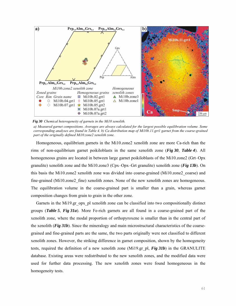
61
Fig 30 Chemical heterogeneity of garnets in the Mi10 xenolith. a) Measured garnet compositions. Averages are always calculated for the largest possible equilibration volume. Some corresponding analyses are found in Table 4. b) Ca distribution map of Mi10b.11.grt1 garnet from the coarse-grained part of the originally defined Mi10.zone2 xenolith zone.
Homogeneous, equilibrium garnets in the Mi10.zone2 xenolith zone are more Ca-rich than the
rims of non-equilibrium garnet poikiloblasts in the same xenolith zone (Fig 30, Table 4). All
homogeneous grains are located in between large garnet poikiloblasts of the Mi10.zone2 (Grt–Opx
granulite) xenolith zone and the Mi10.zone3 (Cpx–Opx–Grt granulite) xenolith zone (Fig 13b). On
this basis the Mi10.zone2 xenolith zone was divided into coarse-grained (Mi10.zone2_coarse) and
fine-grained (Mi10.zone2_fine) xenolith zones. None of the new xenolith zones are homogeneous.
The equilibration volume in the coarse-grained part is smaller than a grain, whereas garnet
composition changes from grain to grain in the other zone.
Garnets in the Mi19.gr_opx_pl xenolith zone can be classified into two compositionally distinct
groups (Table 5, Fig 31a). More Fe-rich garnets are all found in a coarse-grained part of the
xenolith zone, where the modal proportion of orthopyroxene is smaller than in the central part of
the xenolith (Fig 31b). Since the mineralogy and main microstructural characteristics of the coarse-
grained and fine-grained parts are the same, the two parts originally were not classified to different
xenolith zones. However, the striking difference in garnet composition, shown by the homogeneity
tests, required the definition of a new xenolith zone (Mi19.gr_pl, Fig 31b) in the GRANULITE
database. Existing areas were redistributed to the new xenolith zones, and the modified data were
used for further data processing. The new xenolith zones were found homogeneous in the
homogeneity tests.
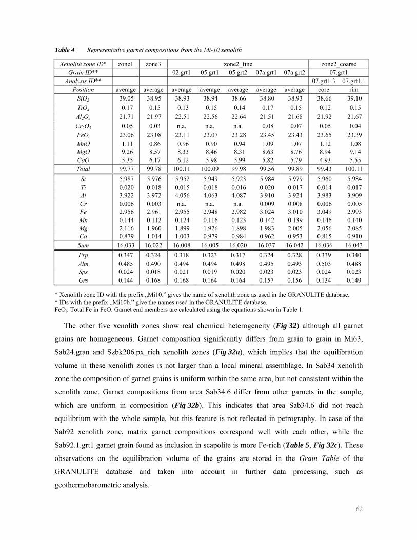
62
Table 4 Representative garnet compositions from the Mi-10 xenolith
Xenolith zone ID* zone1 zone3 zone2_fine zone2_coarse Grain ID** 02.grt1 05.grt1 05.grt2 07a.grt1 07a.grt2 07.grt1
Analysis ID** 07.grt1.3 07.grt1.1Position average average average average average average average core rim
SiO2 39.05 38.95 38.93 38.94 38.66 38.80 38.93 38.66 39.10 TiO2 0.17 0.15 0.13 0.15 0.14 0.17 0.15 0.12 0.15 Al2O3 21.71 21.97 22.51 22.56 22.64 21.51 21.68 21.92 21.67 Cr2O3 0.05 0.03 n.a. n.a. n.a. 0.08 0.07 0.05 0.04 FeOt 23.06 23.08 23.11 23.07 23.28 23.45 23.43 23.65 23.39 MnO 1.11 0.86 0.96 0.90 0.94 1.09 1.07 1.12 1.08 MgO 9.26 8.57 8.33 8.46 8.31 8.63 8.76 8.94 9.14 CaO 5.35 6.17 6.12 5.98 5.99 5.82 5.79 4.93 5.55 Total 99.77 99.78 100.11 100.09 99.98 99.56 99.89 99.43 100.11
Si 5.987 5.976 5.952 5.949 5.923 5.984 5.979 5.960 5.984 Ti 0.020 0.018 0.015 0.018 0.016 0.020 0.017 0.014 0.017 Al 3.922 3.972 4.056 4.063 4.087 3.910 3.924 3.983 3.909 Cr 0.006 0.003 n.a. n.a. n.a. 0.009 0.008 0.006 0.005 Fe 2.956 2.961 2.955 2.948 2.982 3.024 3.010 3.049 2.993 Mn 0.144 0.112 0.124 0.116 0.123 0.142 0.139 0.146 0.140 Mg 2.116 1.960 1.899 1.926 1.898 1.983 2.005 2.056 2.085 Ca 0.879 1.014 1.003 0.979 0.984 0.962 0.953 0.815 0.910
Sum 16.033 16.022 16.008 16.005 16.020 16.037 16.042 16.036 16.043 Prp 0.347 0.324 0.318 0.323 0.317 0.324 0.328 0.339 0.340 Alm 0.485 0.490 0.494 0.494 0.498 0.495 0.493 0.503 0.488 Sps 0.024 0.018 0.021 0.019 0.020 0.023 0.023 0.024 0.023 Grs 0.144 0.168 0.168 0.164 0.164 0.157 0.156 0.134 0.149
* Xenolith zone ID with the prefix „Mi10.” gives the name of xenolith zone as used in the GRANULITE database. * IDs with the prefix „Mi10b.” give the names used in the GRANULITE database. FeOt: Total Fe in FeO. Garnet end members are calculated using the equations shown in Table 1.
The other five xenolith zones show real chemical heterogeneity (Fig 32) although all garnet
grains are homogeneous. Garnet composition significantly differs from grain to grain in Mi63,
Sab24.gran and Szbk206.px_rich xenolith zones (Fig 32a), which implies that the equilibration
volume in these xenolith zones is not larger than a local mineral assemblage. In Sab34 xenolith
zone the composition of garnet grains is uniform within the same area, but not consistent within the
xenolith zone. Garnet compositions from area Sab34.6 differ from other garnets in the sample,
which are uniform in composition (Fig 32b). This indicates that area Sab34.6 did not reach
equilibrium with the whole sample, but this feature is not reflected in petrography. In case of the
Sab92 xenolith zone, matrix garnet compositions correspond well with each other, while the
Sab92.1.grt1 garnet grain found as inclusion in scapolite is more Fe-rich (Table 5, Fig 32c). These
observations on the equilibration volume of the grains are stored in the Grain Table of the
GRANULITE database and taken into account in further data processing, such as
geothermobarometric analysis.
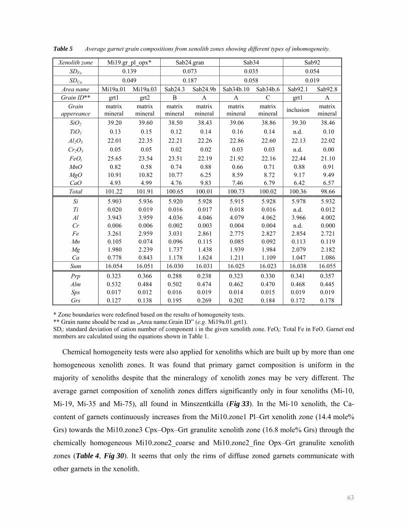
63
Table 5 Average garnet grain compositions from xenolith zones showing different types of inhomogeneity.
Xenolith zone Mi19.gr_pl_opx* Sab24.gran Sab34 Sab92 SDFe 0.139 0.073 0.035 0.054 SDCa 0.049 0.187 0.058 0.019
Area name Mi19a.01 Mi19a.03 Sab24.3 Sab24.9b Sab34b.10 Sab34b.6 Sab92.1 Sab92.8 Grain ID** grt1 grt2 B A A C grt1 A
Grain appereance
matrix mineral
matrix mineral
matrix mineral
matrix mineral
matrix mineral
matrix mineral inclusion matrix
mineral SiO2 39.20 39.60 38.50 38.43 39.06 38.86 39.30 38.46 TiO2 0.13 0.15 0.12 0.14 0.16 0.14 n.d. 0.10 Al2O3 22.01 22.35 22.21 22.26 22.86 22.60 22.13 22.02 Cr2O3 0.05 0.05 0.02 0.02 0.03 0.03 n.d. 0.00 FeOt 25.65 23.54 23.51 22.19 21.92 22.16 22.44 21.10 MnO 0.82 0.58 0.74 0.88 0.66 0.71 0.88 0.91 MgO 10.91 10.82 10.77 6.25 8.59 8.72 9.17 9.49 CaO 4.93 4.99 4.76 9.83 7.46 6.79 6.42 6.57 Total 101.22 101.91 100.65 100.01 100.73 100.02 100.36 98.66
Si 5.903 5.936 5.920 5.928 5.915 5.928 5.978 5.932 Ti 0.020 0.019 0.016 0.017 0.018 0.016 n.d. 0.012 Al 3.943 3.959 4.036 4.046 4.079 4.062 3.966 4.002 Cr 0.006 0.006 0.002 0.003 0.004 0.004 n.d. 0.000 Fe 3.261 2.959 3.031 2.861 2.775 2.827 2.854 2.721 Mn 0.105 0.074 0.096 0.115 0.085 0.092 0.113 0.119 Mg 1.980 2.239 1.737 1.438 1.939 1.984 2.079 2.182 Ca 0.778 0.843 1.178 1.624 1.211 1.109 1.047 1.086
Sum 16.054 16.051 16.030 16.031 16.025 16.023 16.038 16.055 Prp 0.323 0.366 0.288 0.238 0.323 0.330 0.341 0.357 Alm 0.532 0.484 0.502 0.474 0.462 0.470 0.468 0.445 Sps 0.017 0.012 0.016 0.019 0.014 0.015 0.019 0.019 Grs 0.127 0.138 0.195 0.269 0.202 0.184 0.172 0.178
* Zone boundaries were redefined based on the results of homogeneity tests. ** Grain name should be read as „Area name.Grain ID” (e.g. Mi19a.01.grt1). SDi: standard deviation of cation number of component i in the given xenolith zone. FeOt: Total Fe in FeO. Garnet end members are calculated using the equations shown in Table 1.
Chemical homogeneity tests were also applied for xenoliths which are built up by more than one
homogeneous xenolith zones. It was found that primary garnet composition is uniform in the
majority of xenoliths despite that the mineralogy of xenolith zones may be very different. The
average garnet composition of xenolith zones differs significantly only in four xenoliths (Mi-10,
Mi-19, Mi-35 and Mi-75), all found in Minszentkálla (Fig 33). In the Mi-10 xenolith, the Ca-
content of garnets continuously increases from the Mi10.zone1 Pl–Grt xenolith zone (14.4 mole%
Grs) towards the Mi10.zone3 Cpx–Opx–Grt granulite xenolith zone (16.8 mole% Grs) through the
chemically homogeneous Mi10.zone2_coarse and Mi10.zone2_fine Opx–Grt granulite xenolith
zones (Table 4, Fig 30). It seems that only the rims of diffuse zoned garnets communicate with
other garnets in the xenolith.
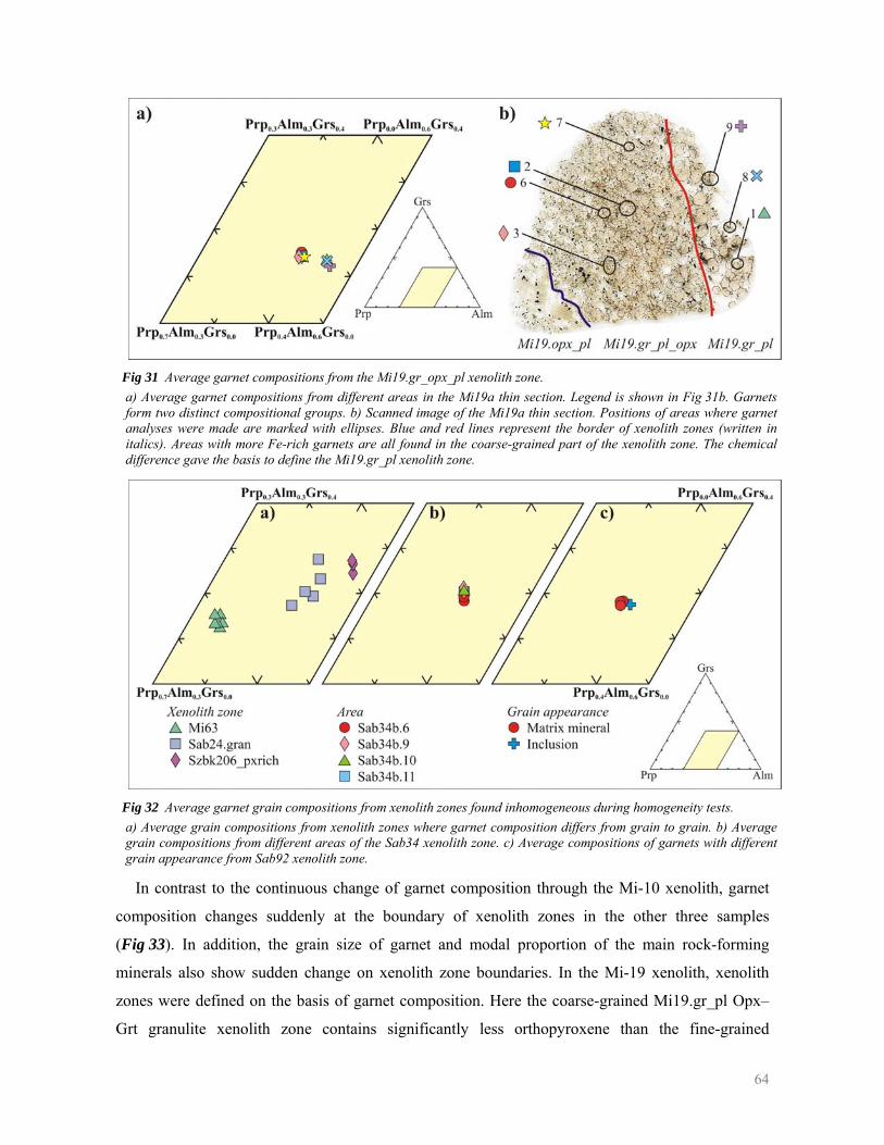
64
Fig 31 Average garnet compositions from the Mi19.gr_opx_pl xenolith zone. a) Average garnet compositions from different areas in the Mi19a thin section. Legend is shown in Fig 31b. Garnets form two distinct compositional groups. b) Scanned image of the Mi19a thin section. Positions of areas where garnet analyses were made are marked with ellipses. Blue and red lines represent the border of xenolith zones (written in italics). Areas with more Fe-rich garnets are all found in the coarse-grained part of the xenolith zone. The chemical difference gave the basis to define the Mi19.gr_pl xenolith zone.
Fig 32 Average garnet grain compositions from xenolith zones found inhomogeneous during homogeneity tests. a) Average grain compositions from xenolith zones where garnet composition differs from grain to grain. b) Average grain compositions from different areas of the Sab34 xenolith zone. c) Average compositions of garnets with different grain appearance from Sab92 xenolith zone.
In contrast to the continuous change of garnet composition through the Mi-10 xenolith, garnet
composition changes suddenly at the boundary of xenolith zones in the other three samples
(Fig 33). In addition, the grain size of garnet and modal proportion of the main rock-forming
minerals also show sudden change on xenolith zone boundaries. In the Mi-19 xenolith, xenolith
zones were defined on the basis of garnet composition. Here the coarse-grained Mi19.gr_pl Opx–
Grt granulite xenolith zone contains significantly less orthopyroxene than the fine-grained
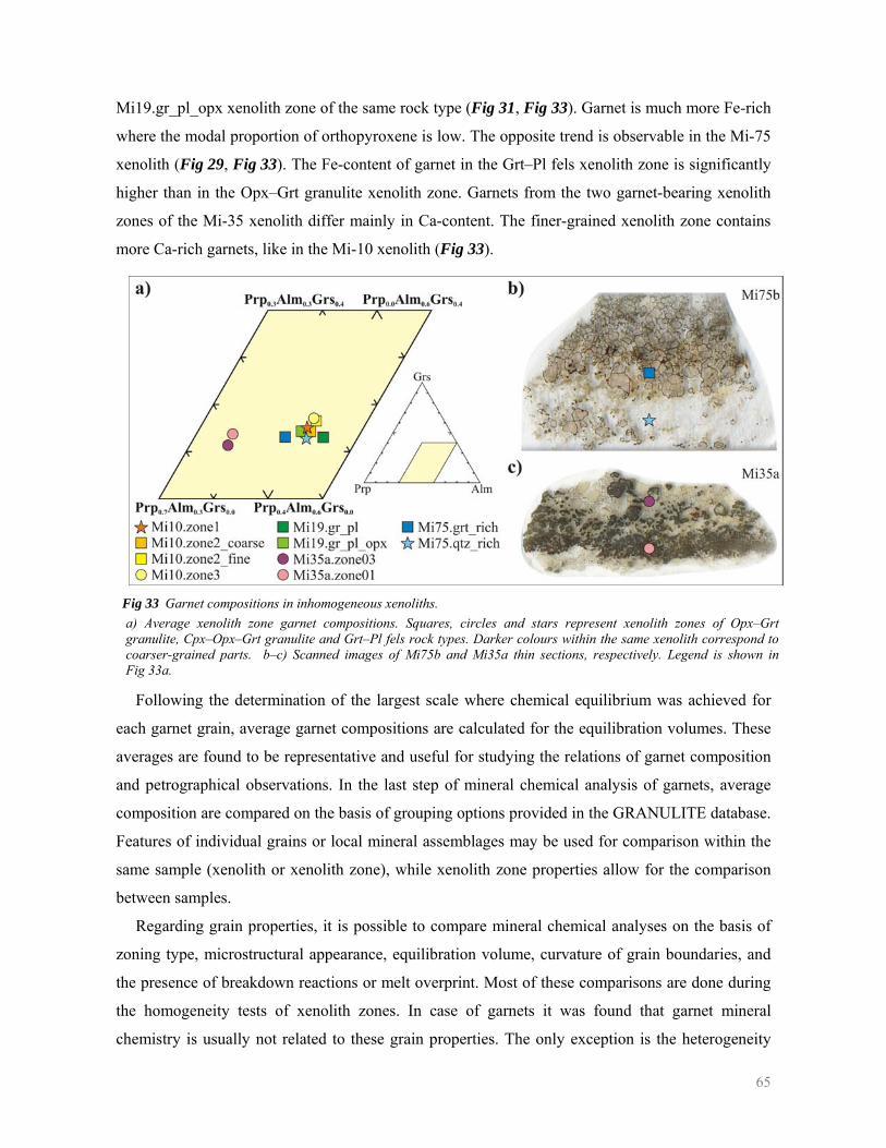
65
Mi19.gr_pl_opx xenolith zone of the same rock type (Fig 31, Fig 33). Garnet is much more Fe-rich
where the modal proportion of orthopyroxene is low. The opposite trend is observable in the Mi-75
xenolith (Fig 29, Fig 33). The Fe-content of garnet in the Grt–Pl fels xenolith zone is significantly
higher than in the Opx–Grt granulite xenolith zone. Garnets from the two garnet-bearing xenolith
zones of the Mi-35 xenolith differ mainly in Ca-content. The finer-grained xenolith zone contains
more Ca-rich garnets, like in the Mi-10 xenolith (Fig 33).
Fig 33 Garnet compositions in inhomogeneous xenoliths. a) Average xenolith zone garnet compositions. Squares, circles and stars represent xenolith zones of Opx–Grt granulite, Cpx–Opx–Grt granulite and Grt–Pl fels rock types. Darker colours within the same xenolith correspond to coarser-grained parts. b–c) Scanned images of Mi75b and Mi35a thin sections, respectively. Legend is shown in Fig 33a.
Following the determination of the largest scale where chemical equilibrium was achieved for
each garnet grain, average garnet compositions are calculated for the equilibration volumes. These
averages are found to be representative and useful for studying the relations of garnet composition
and petrographical observations. In the last step of mineral chemical analysis of garnets, average
composition are compared on the basis of grouping options provided in the GRANULITE database.
Features of individual grains or local mineral assemblages may be used for comparison within the
same sample (xenolith or xenolith zone), while xenolith zone properties allow for the comparison
between samples.
Regarding grain properties, it is possible to compare mineral chemical analyses on the basis of
zoning type, microstructural appearance, equilibration volume, curvature of grain boundaries, and
the presence of breakdown reactions or melt overprint. Most of these comparisons are done during
the homogeneity tests of xenolith zones. In case of garnets it was found that garnet mineral
chemistry is usually not related to these grain properties. The only exception is the heterogeneity
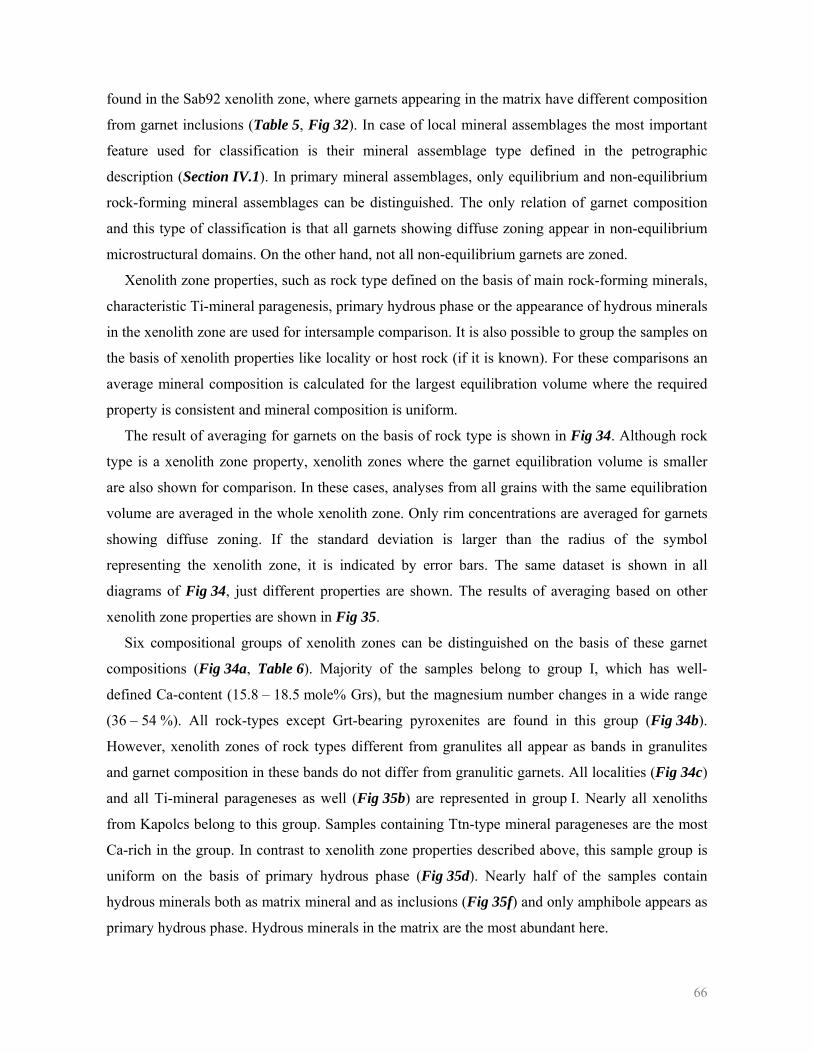
66
found in the Sab92 xenolith zone, where garnets appearing in the matrix have different composition
from garnet inclusions (Table 5, Fig 32). In case of local mineral assemblages the most important
feature used for classification is their mineral assemblage type defined in the petrographic
description (Section IV.1). In primary mineral assemblages, only equilibrium and non-equilibrium
rock-forming mineral assemblages can be distinguished. The only relation of garnet composition
and this type of classification is that all garnets showing diffuse zoning appear in non-equilibrium
microstructural domains. On the other hand, not all non-equilibrium garnets are zoned.
Xenolith zone properties, such as rock type defined on the basis of main rock-forming minerals,
characteristic Ti-mineral paragenesis, primary hydrous phase or the appearance of hydrous minerals
in the xenolith zone are used for intersample comparison. It is also possible to group the samples on
the basis of xenolith properties like locality or host rock (if it is known). For these comparisons an
average mineral composition is calculated for the largest equilibration volume where the required
property is consistent and mineral composition is uniform.
The result of averaging for garnets on the basis of rock type is shown in Fig 34. Although rock
type is a xenolith zone property, xenolith zones where the garnet equilibration volume is smaller
are also shown for comparison. In these cases, analyses from all grains with the same equilibration
volume are averaged in the whole xenolith zone. Only rim concentrations are averaged for garnets
showing diffuse zoning. If the standard deviation is larger than the radius of the symbol
representing the xenolith zone, it is indicated by error bars. The same dataset is shown in all
diagrams of Fig 34, just different properties are shown. The results of averaging based on other
xenolith zone properties are shown in Fig 35.
Six compositional groups of xenolith zones can be distinguished on the basis of these garnet
compositions (Fig 34a, Table 6). Majority of the samples belong to group I, which has well-
defined Ca-content (15.8 – 18.5 mole% Grs), but the magnesium number changes in a wide range
(36 – 54 %). All rock-types except Grt-bearing pyroxenites are found in this group (Fig 34b).
However, xenolith zones of rock types different from granulites all appear as bands in granulites
and garnet composition in these bands do not differ from granulitic garnets. All localities (Fig 34c)
and all Ti-mineral parageneses as well (Fig 35b) are represented in group I. Nearly all xenoliths
from Kapolcs belong to this group. Samples containing Ttn-type mineral parageneses are the most
Ca-rich in the group. In contrast to xenolith zone properties described above, this sample group is
uniform on the basis of primary hydrous phase (Fig 35d). Nearly half of the samples contain
hydrous minerals both as matrix mineral and as inclusions (Fig 35f) and only amphibole appears as
primary hydrous phase. Hydrous minerals in the matrix are the most abundant here.
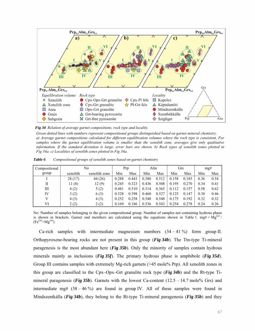
67
Fig 34 Relation of average garnet compositions, rock type and locality. Green dotted lines with numbers represent compositional groups distinguished based on garnet mineral chemistry. a) Average garnet compositions calculated for different equilibration volumes where the rock type is consistent. For samples where the garnet equilibration volume is smaller than the xenolith zone, averages give only qualitative information. If the standard deviation is large, error bars are shown. b) Rock types of xenolith zones plotted in Fig 34a. c) Localities of xenolith zones plotted in Fig 34a.
Table 6 Compositional groups of xenolith zones based on garnet chemistry
No Prp Alm Grs mg# Compositional group xenolith xenolith zone Min Max Min Max Min Max Min Max
I 28 (17) 44 (26) 0.288 0.443 0.380 0.512 0.158 0.185 0.36 0.54 II 11 (8) 12 (9) 0.245 0.323 0.436 0.508 0.195 0.270 0.34 0.41 III 4 (2) 5 (2) 0.481 0.510 0.314 0.365 0.112 0.157 0.58 0.62 IV 3 (2) 6 (3) 0.328 0.398 0.460 0.527 0.125 0.147 0.38 0.46 V 4 (3) 4 (3) 0.252 0.258 0.540 0.548 0.175 0.192 0.32 0.32 VI 2 (2) 2 (2) 0.169 0.186 0.536 0.543 0.254 0.278 0.24 0.26
No: Number of samples belonging to the given compositional group. Number of samples not containing hydrous phase is shown in brackets. Garnet end members are calculated using the equations shown in Table 1. mg# = MgGrt / (FeGrt+MgGrt).
Ca-rich samples with intermediate magnesium numbers (34 – 41 %) form group II.
Orthopyroxene-bearing rocks are not present in this group (Fig 34b). The Ttn-type Ti-mineral
paragenesis is the most abundant here (Fig 35b). Only the minority of samples contain hydrous
minerals mainly as inclusions (Fig 35f). The primary hydrous phase is amphibole (Fig 35d).
Group III contains samples with extremely Mg-rich garnets (>45 mole% Prp). All xenolith zones in
this group are classified to the Cpx–Opx–Grt granulite rock type (Fig 34b) and the Rt-type Ti-
mineral paragenesis (Fig 35b). Garnets with the lowest Ca-content (12.5 – 14.7 mole% Grs) and
intermediate mg# (38 – 46 %) are found in group IV. All of these samples were found in
Mindszentkálla (Fig 34b), they belong to the Rt-type Ti-mineral paragenesis (Fig 35b) and they
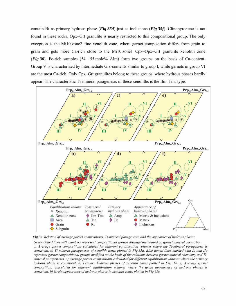
68
contain Bt as primary hydrous phase (Fig 35d) just as inclusions (Fig 35f). Clinopyroxene is not
found in these rocks. Opx–Grt granulite is nearly restricted to this compositional group. The only
exception is the Mi10.zone2_fine xenolith zone, where garnet composition differs from grain to
grain and gets more Ca-rich close to the Mi10.zone1 Cpx–Opx–Grt granulite xenolith zone
(Fig 30). Fe-rich samples (54 – 55 mole% Alm) form two groups on the basis of Ca-content.
Group V is characterized by intermediate Grs-contents similar to group I, while garnets in group VI
are the most Ca-rich. Only Cpx–Grt granulites belong to these groups, where hydrous phases hardly
appear. The characteristic Ti-mineral paragenesis of these xenoliths is the Ilm–Tmt-type.
Fig 35 Relation of average garnet compositions, Ti-mineral parageneses and the appearnce of hydrous phases. Green dotted lines with numbers represent compositional groups distinguished based on garnet mineral chemistry. a) Average garnet compositions calculated for different equilibration volumes where the Ti-mineral paragenesis is consistent. b) Ti-mineral parageneses of xenolith zones plotted in Fig 35a. Blue dotted lines marked with Ia and IIa represent garnet compositional groups modified on the basis of the relations between garnet mineral chemistry and Ti-mineral parageneses. c) Average garnet compositions calculated for different equilibration volumes where the primary hydrous phase is consistent. b) Primary hydrous phases of xenolith zones plotted in Fig 35b. e) Average garnet compositions calculated for different equilibration volumes where the grain appearance of hydrous phases is consistent. b) Grain appearance of hydrous phases in xenolith zones plotted in Fig 35c.
69
As a feedback to the GRANULITE database (Fig 11), a new xenolith zone property (GrtGroup
Field in the XenolithZone Table) was defined, which is related to garnet chemistry in the samples.
Xenolith zones were classified to the compositional groups described above. Since then, this
property is also available for mineral chemical analysis.
IV.2.1.2 Plagioclase
Mineral chemical data from 249 primary plagioclase grains have been collected in this work. All
analyses grouped by xenoliths are listed in the MineralChemistry_Pl.pdf mineral chemistry report,
which is attached electronically to the thesis.
In general, plagioclase grains are solid solutions of albite and anorthite with minor orthoclase
content (<6.8 mole%). According to zoning analyses, most plagioclase grains are homogeneous in
composition or they show only growth zoning (further described in Section IV.2.2.1). Diffusion or
complex zoning was detected in 18 grains from 12 xenoliths. The observed zoning patterns are
usually effected by the interaction with the host melt. The identification of processes resulting in
these zoning types requires detailed high resolution electron beam microanalytical studies. Since
plagioclase grains, showing diffuse and complex zoning are not characteristic for the xenolith zones
in which they appear and detailed description of zoning patterns exceeds the limits of this study,
analyses from these grains are not included in further data processing.
During homogeneity tests, four xenolith zones were found to be inhomogeneous (Fig 36a) on
the basis of plagioclase composition. The equilibration volume in the Mi-19 xenolith corresponds
to a local mineral assemblage, while plagioclase composition changes from grain to grain in Sab82
and NT2 xenolith zones. Besides these, two more samples (Mi-10 and Mi-75) were found to be
inhomogeneous on the xenolith level (Fig 36a). In the Mi-10 xenolith the Ca-content of plagioclase
increases continuously from the Pl–Grt fels xenolith zone (Mi10.zone1) towards the Cpx–Opx–Grt
granulite xenolith zone (Mi10.zone3) through the Opx–Grt granulite xenolith zones similarly to the
compositional change in garnet (Fig 30). The plagioclase composition in the Mi-75 xenolith also
changes in the same way from Pl–Grt fels towards Opx–Grt granulite.
Primary plagioclase grains are of intermediate composition (Ab0.35-0.60An0.37-0.63Or0.00-0.04,
Fig 36b–f). Clinopyroxene-bearing Grt granulites are found in the whole compositional range.
However, Opx–Grt granulites, Pl–Grt and Cpx–Pl felses are more albite-rich (Ab>50 mole%,
Fig 36c). Plagioclase inclusions in pyroxenites also have similar composition. There are no clear
relations between plagioclase compositions and observed Ti-mineral parageneses (Fig 36d) or
primary hydrous phase (Fig 36e). In samples, where garnets have low Ca-content (Group IV),
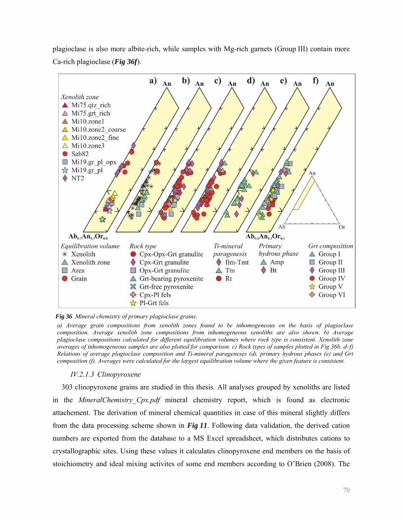
70
plagioclase is also more albite-rich, while samples with Mg-rich garnets (Group III) contain more
Ca-rich plagioclase (Fig 36f).
Fig 36 Mineral chemistry of primary plagioclase grains. a) Average grain compositions from xenolith zones found to be inhomogeneous on the basis of plagioclase composition. Average xenolith zone compositions from inhomogeneous xenoliths are also shown. b) Average plagioclase compositions calculated for different equilibration volumes where rock type is consistent. Xenolith zone averages of inhomogeneous samples are also plotted for comparison. c) Rock types of samples plotted in Fig 36b. d–f) Relations of average plagioclase composition and Ti-mineral parageneses (d), primary hydrous phases (e) and Grt composition (f). Averages were calculated for the largest equilibration volume where the given feature is consistent.
IV.2.1.3 Clinopyroxene
303 clinopyroxene grains are studied in this thesis. All analyses grouped by xenoliths are listed
in the MineralChemistry_Cpx.pdf mineral chemistry report, which is found as electronic
attachement. The derivation of mineral chemical quantities in case of this mineral slightly differs
from the data processing scheme shown in Fig 11. Following data validation, the derived cation
numbers are exported from the database to a MS Excel spreadsheet, which distributes cations to
crystallographic sites. Using these values it calculates clinopyroxene end members on the basis of
stoichiometry and ideal mixing activites of some end members according to O’Brien (2008). The
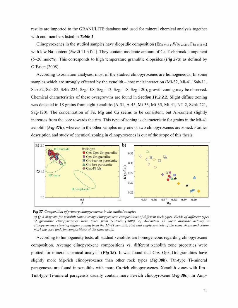
71
results are imported to the GRANULITE database and used for mineral chemical analysis together
with end members listed in Table 1.
Clinopyroxenes in the studied samples have diopsidic composition (En0.29-0.43Wo0.40-0.50Fs0.11-0.25)
with low Na-content (Na<0.11 p.f.u.). They contain moderate amount of Ca-Tschermak component
(5–20 mole%). This corresponds to high temperature granulitic diopsides (Fig 37a) as defined by
O’Brien (2008).
According to zonation analyses, most of the studied clinopyroxenes are homogeneous. In some
samples which are strongly effected by the xenolith – host melt interaction (Mi-32, Mi-41, Sab-11,
Sab-52, Sab-82, Szbk-224, Szg-108, Szg-113, Szg-118, Szg-120), growth zoning may be observed.
Chemical characteristics of these overgrowths are found in Section IV.2.2.2. Slight diffuse zoning
was detected in 18 grains from eight xenoliths (A-31, A-45, Mi-33, Mi-35, Mi-41, NT-2, Szbk-221,
Szg-120). The concentration of Fe, Mg and Ca seems to be consistent, but Al-content slightly
increases from the core towards the rim. This type of zoning is characteristic for grains in the Mi-41
xenolith (Fig 37b), whereas in the other samples only one or two clinopyroxenes are zoned. Further
description and study of chemical zoning in clinopyroxenes is out of the scope of this thesis.
Fig 37 Composition of primary clinopyroxenes in the studied samples a) Q–J diagram for xenolith zone average clinopyroxene compositions of different rock types. Fields of different types of granulitic clinopyroxenes were taken from O’Brien (2008). b) Al-content vs. ideal diopside activity in clinopyroxenes showing diffuse zoning from the Mi-41 xenolith. Full and empty symbols of the same shape and colour mark the core and rim compositions of the same grain.
According to homogeneity tests, all studied xenoliths are homogeneous regarding clinopyroxene
composition. Average clinopyroxene compositions vs. different xenolith zone properties were
plotted for mineral chemical analysis (Fig 38). It was found that Cpx–Opx–Grt granulites have
slightly more Mg-rich clinopyroxenes than other rock types (Fig 38b). Ttn-type Ti-mineral
parageneses are found in xenoliths with more Ca-rich clinopyroxenes. Xenolith zones with Ilm–
Tmt-type Ti-mineral paragensis usually contain more Fe-rich clinopyroxene (Fig 38c). In Amp-
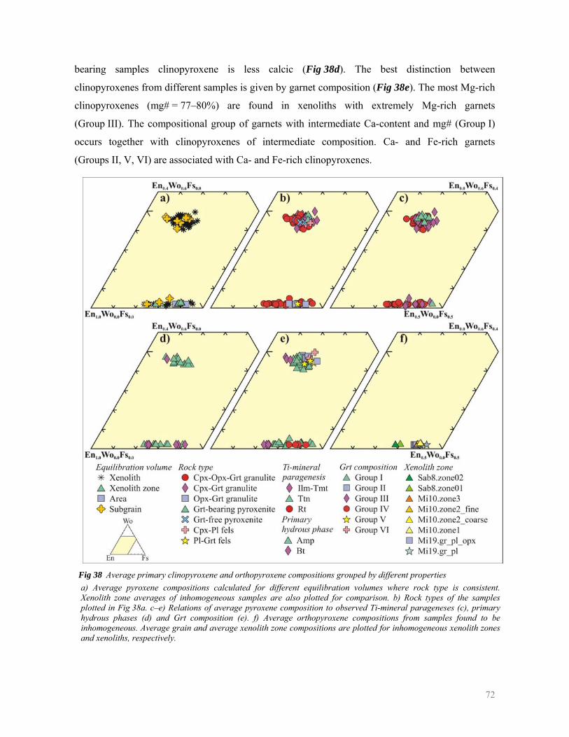
72
bearing samples clinopyroxene is less calcic (Fig 38d). The best distinction between
clinopyroxenes from different samples is given by garnet composition (Fig 38e). The most Mg-rich
clinopyroxenes (mg# = 77–80%) are found in xenoliths with extremely Mg-rich garnets
(Group III). The compositional group of garnets with intermediate Ca-content and mg# (Group I)
occurs together with clinopyroxenes of intermediate composition. Ca- and Fe-rich garnets
(Groups II, V, VI) are associated with Ca- and Fe-rich clinopyroxenes.
Fig 38 Average primary clinopyroxene and orthopyroxene compositions grouped by different properties a) Average pyroxene compositions calculated for different equilibration volumes where rock type is consistent. Xenolith zone averages of inhomogeneous samples are also plotted for comparison. b) Rock types of the samples plotted in Fig 38a. c–e) Relations of average pyroxene composition to observed Ti-mineral parageneses (c), primary hydrous phases (d) and Grt composition (e). f) Average orthopyroxene compositions from samples found to be inhomogeneous. Average grain and average xenolith zone compositions are plotted for inhomogeneous xenolith zones and xenoliths, respectively.
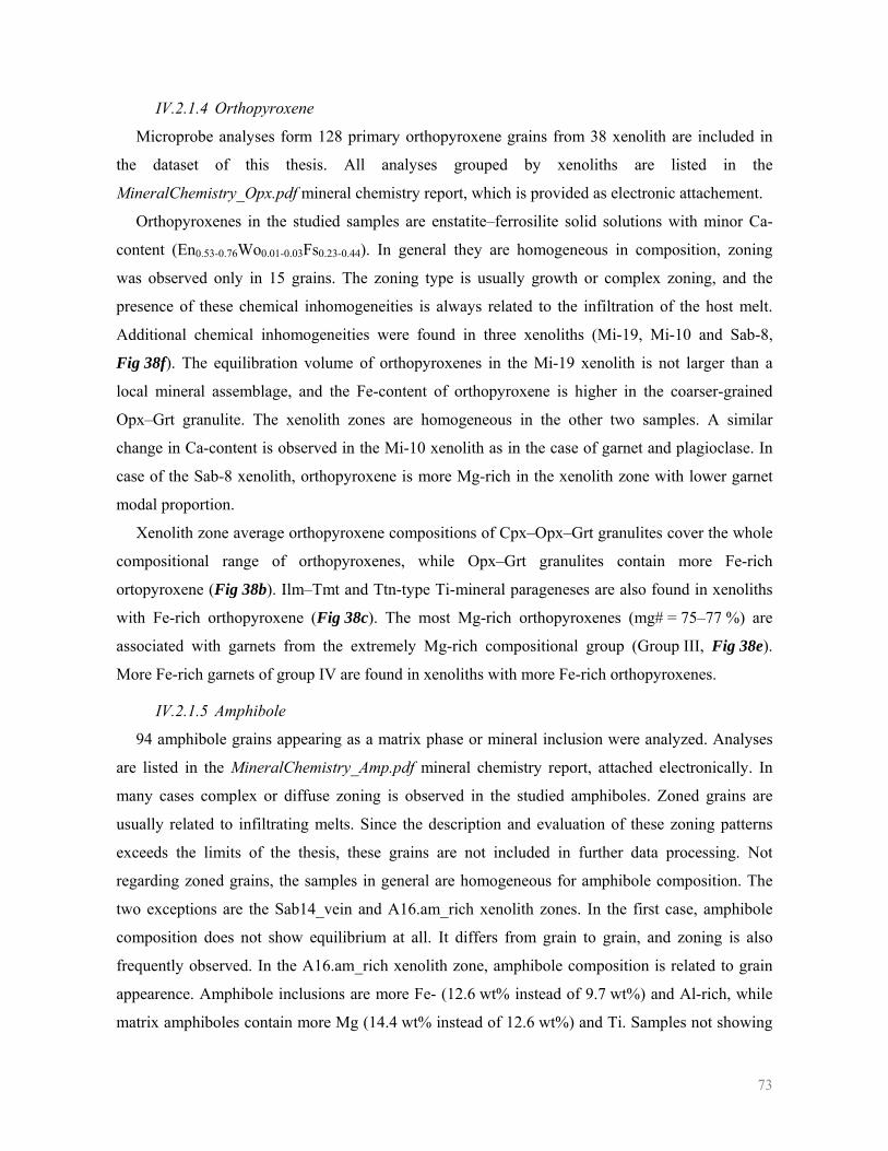
73
IV.2.1.4 Orthopyroxene
Microprobe analyses form 128 primary orthopyroxene grains from 38 xenolith are included in
the dataset of this thesis. All analyses grouped by xenoliths are listed in the
MineralChemistry_Opx.pdf mineral chemistry report, which is provided as electronic attachement.
Orthopyroxenes in the studied samples are enstatite–ferrosilite solid solutions with minor Ca-
content (En0.53-0.76Wo0.01-0.03Fs0.23-0.44). In general they are homogeneous in composition, zoning
was observed only in 15 grains. The zoning type is usually growth or complex zoning, and the
presence of these chemical inhomogeneities is always related to the infiltration of the host melt.
Additional chemical inhomogeneities were found in three xenoliths (Mi-19, Mi-10 and Sab-8,
Fig 38f). The equilibration volume of orthopyroxenes in the Mi-19 xenolith is not larger than a
local mineral assemblage, and the Fe-content of orthopyroxene is higher in the coarser-grained
Opx–Grt granulite. The xenolith zones are homogeneous in the other two samples. A similar
change in Ca-content is observed in the Mi-10 xenolith as in the case of garnet and plagioclase. In
case of the Sab-8 xenolith, orthopyroxene is more Mg-rich in the xenolith zone with lower garnet
modal proportion.
Xenolith zone average orthopyroxene compositions of Cpx–Opx–Grt granulites cover the whole
compositional range of orthopyroxenes, while Opx–Grt granulites contain more Fe-rich
ortopyroxene (Fig 38b). Ilm–Tmt and Ttn-type Ti-mineral parageneses are also found in xenoliths
with Fe-rich orthopyroxene (Fig 38c). The most Mg-rich orthopyroxenes (mg# = 75–77 %) are
associated with garnets from the extremely Mg-rich compositional group (Group III, Fig 38e).
More Fe-rich garnets of group IV are found in xenoliths with more Fe-rich orthopyroxenes.
IV.2.1.5 Amphibole
94 amphibole grains appearing as a matrix phase or mineral inclusion were analyzed. Analyses
are listed in the MineralChemistry_Amp.pdf mineral chemistry report, attached electronically. In
many cases complex or diffuse zoning is observed in the studied amphiboles. Zoned grains are
usually related to infiltrating melts. Since the description and evaluation of these zoning patterns
exceeds the limits of the thesis, these grains are not included in further data processing. Not
regarding zoned grains, the samples in general are homogeneous for amphibole composition. The
two exceptions are the Sab14_vein and A16.am_rich xenolith zones. In the first case, amphibole
composition does not show equilibrium at all. It differs from grain to grain, and zoning is also
frequently observed. In the A16.am_rich xenolith zone, amphibole composition is related to grain
appearence. Amphibole inclusions are more Fe- (12.6 wt% instead of 9.7 wt%) and Al-rich, while
matrix amphiboles contain more Mg (14.4 wt% instead of 12.6 wt%) and Ti. Samples not showing
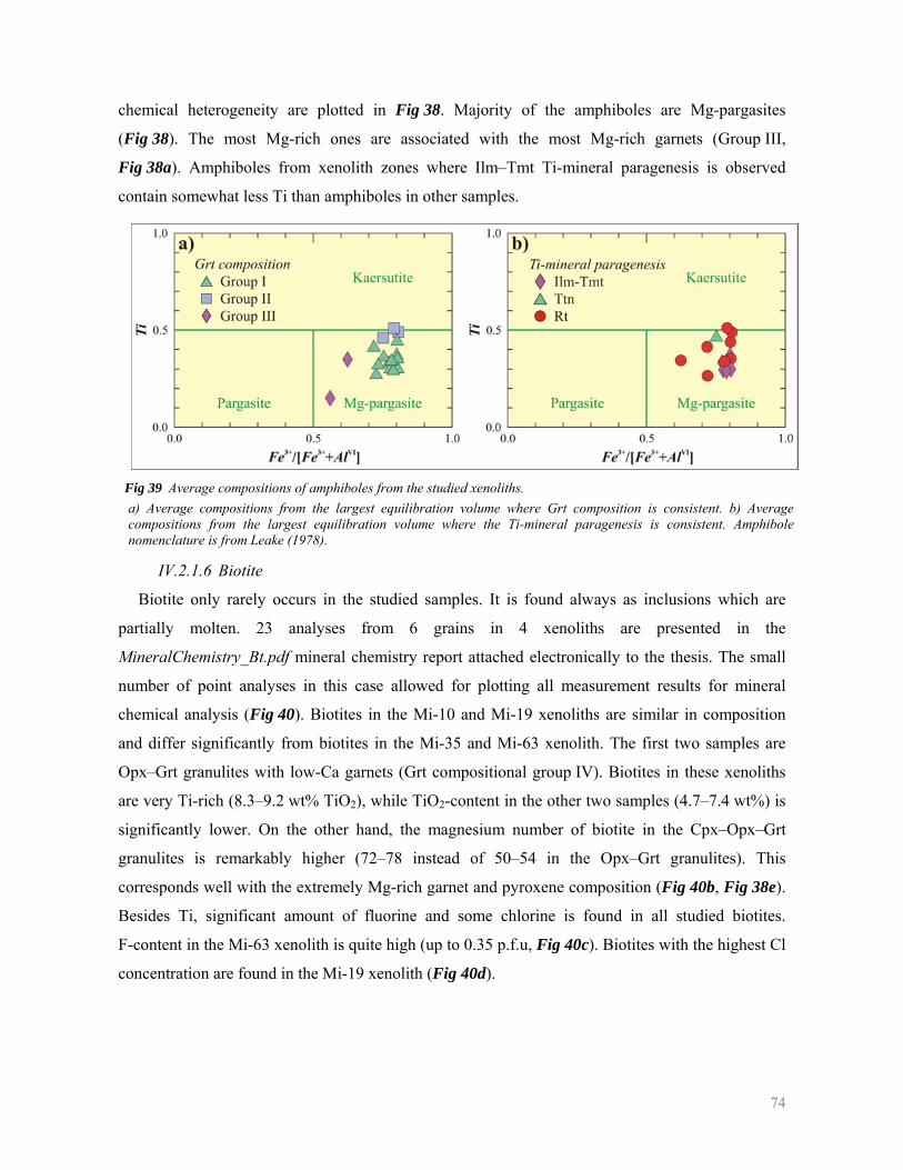
74
chemical heterogeneity are plotted in Fig 38. Majority of the amphiboles are Mg-pargasites
(Fig 38). The most Mg-rich ones are associated with the most Mg-rich garnets (Group III,
Fig 38a). Amphiboles from xenolith zones where Ilm–Tmt Ti-mineral paragenesis is observed
contain somewhat less Ti than amphiboles in other samples.
Fig 39 Average compositions of amphiboles from the studied xenoliths. a) Average compositions from the largest equilibration volume where Grt composition is consistent. b) Average compositions from the largest equilibration volume where the Ti-mineral paragenesis is consistent. Amphibole nomenclature is from Leake (1978).
IV.2.1.6 Biotite
Biotite only rarely occurs in the studied samples. It is found always as inclusions which are
partially molten. 23 analyses from 6 grains in 4 xenoliths are presented in the
MineralChemistry_Bt.pdf mineral chemistry report attached electronically to the thesis. The small
number of point analyses in this case allowed for plotting all measurement results for mineral
chemical analysis (Fig 40). Biotites in the Mi-10 and Mi-19 xenoliths are similar in composition
and differ significantly from biotites in the Mi-35 and Mi-63 xenolith. The first two samples are
Opx–Grt granulites with low-Ca garnets (Grt compositional group IV). Biotites in these xenoliths
are very Ti-rich (8.3–9.2 wt% TiO2), while TiO2-content in the other two samples (4.7–7.4 wt%) is
significantly lower. On the other hand, the magnesium number of biotite in the Cpx–Opx–Grt
granulites is remarkably higher (72–78 instead of 50–54 in the Opx–Grt granulites). This
corresponds well with the extremely Mg-rich garnet and pyroxene composition (Fig 40b, Fig 38e).
Besides Ti, significant amount of fluorine and some chlorine is found in all studied biotites.
F-content in the Mi-63 xenolith is quite high (up to 0.35 p.f.u, Fig 40c). Biotites with the highest Cl
concentration are found in the Mi-19 xenolith (Fig 40d).
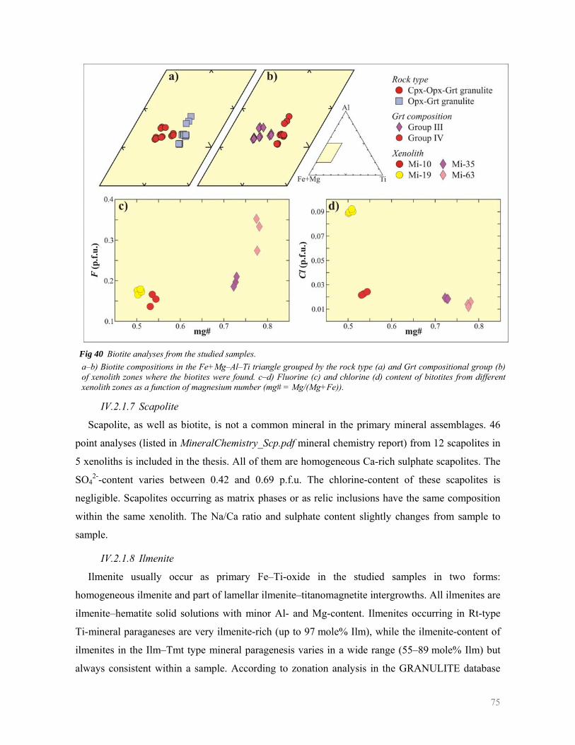
75
Fig 40 Biotite analyses from the studied samples. a–b) Biotite compositions in the Fe+Mg–Al–Ti triangle grouped by the rock type (a) and Grt compositional group (b) of xenolith zones where the biotites were found. c–d) Fluorine (c) and chlorine (d) content of bitotites from different xenolith zones as a function of magnesium number (mg# = Mg/(Mg+Fe)).
IV.2.1.7 Scapolite
Scapolite, as well as biotite, is not a common mineral in the primary mineral assemblages. 46
point analyses (listed in MineralChemistry_Scp.pdf mineral chemistry report) from 12 scapolites in
5 xenoliths is included in the thesis. All of them are homogeneous Ca-rich sulphate scapolites. The
SO42--content varies between 0.42 and 0.69 p.f.u. The chlorine-content of these scapolites is
negligible. Scapolites occurring as matrix phases or as relic inclusions have the same composition
within the same xenolith. The Na/Ca ratio and sulphate content slightly changes from sample to
sample.
IV.2.1.8 Ilmenite
Ilmenite usually occur as primary Fe–Ti-oxide in the studied samples in two forms:
homogeneous ilmenite and part of lamellar ilmenite–titanomagnetite intergrowths. All ilmenites are
ilmenite–hematite solid solutions with minor Al- and Mg-content. Ilmenites occurring in Rt-type
Ti-mineral paraganeses are very ilmenite-rich (up to 97 mole% Ilm), while the ilmenite-content of
ilmenites in the Ilm–Tmt type mineral paragenesis varies in a wide range (55–89 mole% Ilm) but
always consistent within a sample. According to zonation analysis in the GRANULITE database
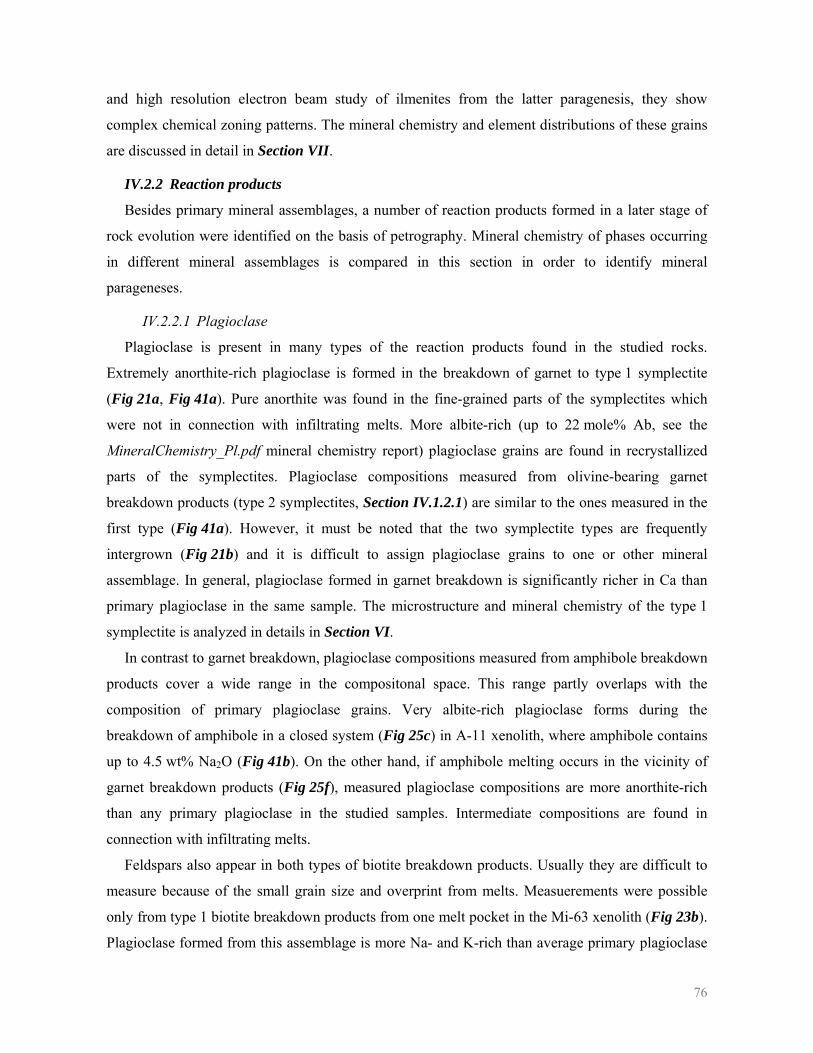
76
and high resolution electron beam study of ilmenites from the latter paragenesis, they show
complex chemical zoning patterns. The mineral chemistry and element distributions of these grains
are discussed in detail in Section VII.
IV.2.2 Reaction products
Besides primary mineral assemblages, a number of reaction products formed in a later stage of
rock evolution were identified on the basis of petrography. Mineral chemistry of phases occurring
in different mineral assemblages is compared in this section in order to identify mineral
parageneses.
IV.2.2.1 Plagioclase
Plagioclase is present in many types of the reaction products found in the studied rocks.
Extremely anorthite-rich plagioclase is formed in the breakdown of garnet to type 1 symplectite
(Fig 21a, Fig 41a). Pure anorthite was found in the fine-grained parts of the symplectites which
were not in connection with infiltrating melts. More albite-rich (up to 22 mole% Ab, see the
MineralChemistry_Pl.pdf mineral chemistry report) plagioclase grains are found in recrystallized
parts of the symplectites. Plagioclase compositions measured from olivine-bearing garnet
breakdown products (type 2 symplectites, Section IV.1.2.1) are similar to the ones measured in the
first type (Fig 41a). However, it must be noted that the two symplectite types are frequently
intergrown (Fig 21b) and it is difficult to assign plagioclase grains to one or other mineral
assemblage. In general, plagioclase formed in garnet breakdown is significantly richer in Ca than
primary plagioclase in the same sample. The microstructure and mineral chemistry of the type 1
symplectite is analyzed in details in Section VI.
In contrast to garnet breakdown, plagioclase compositions measured from amphibole breakdown
products cover a wide range in the compositonal space. This range partly overlaps with the
composition of primary plagioclase grains. Very albite-rich plagioclase forms during the
breakdown of amphibole in a closed system (Fig 25c) in A-11 xenolith, where amphibole contains
up to 4.5 wt% Na2O (Fig 41b). On the other hand, if amphibole melting occurs in the vicinity of
garnet breakdown products (Fig 25f), measured plagioclase compositions are more anorthite-rich
than any primary plagioclase in the studied samples. Intermediate compositions are found in
connection with infiltrating melts.
Feldspars also appear in both types of biotite breakdown products. Usually they are difficult to
measure because of the small grain size and overprint from melts. Measuerements were possible
only from type 1 biotite breakdown products from one melt pocket in the Mi-63 xenolith (Fig 23b).
Plagioclase formed from this assemblage is more Na- and K-rich than average primary plagioclase
77
grains from the xenolith (Fig 41b). A K-feldspar (Ab0.20An0.04Or0.76) was also found in this melt
pocket as inclusion.
Fig 41 Composition of plagioclase grains appearing as different reaction products in the xenoliths. Green dotted line borders the compositional range of average primary plagioclase compositions shown in Fig 36. All plotted compositions are averages calculated for the largest equilibration volume of the given mineral assemblage. Primary plagioclase compositions from selected xenoliths are also shown for comparison. Symbols of primary plagioclase compositions have the same shape as their rock type symbol in Fig 36. a) Plagioclase compositions measured from type 1 and type 2 symplectites after garnet. b) Plagioclase compositions from biotite and amphibole breakdown products. c) Plagioclase composition from Cpx–Ilm–Pl symplectites after titanite breakdown. d) Plagioclase compositions from scapolite breakdown products. e) Composition of plagioclase overgrowths. f) Plagioclase composition from infiltrating host melt crystallized in the xenoliths.
Plagioclase grains in Cpx–Ilm–Pl symplectites formed in type 1 titanite breakdown covers a
wide compositional change (Fig 41e). Usually the composition of primary plagioclase and
plagioclase formed from titanite breakdown is different, but the deviation is not systematic. In the
Sab-82 xenolith, the plagioclase composition differs in each symplectite. The plagioclase
intergrown with clinopyroxene and ilmenite (Fig 27c) has very similar composition to primary
plagioclase, whilst another grain which hosts a Cpx–Ilm symplectite (Fig 27b) is more anorthite-
rich. In general, the composition of plagioclase grains from more equilibrated microstructures is
closer to the primary plagioclase composition.
Plagioclase formed during scapolite breakdown is always more anorthite-rich than primary
plagioclase grains (Fig 41d), but their anorthite-content is not as high as in plagioclase grains from
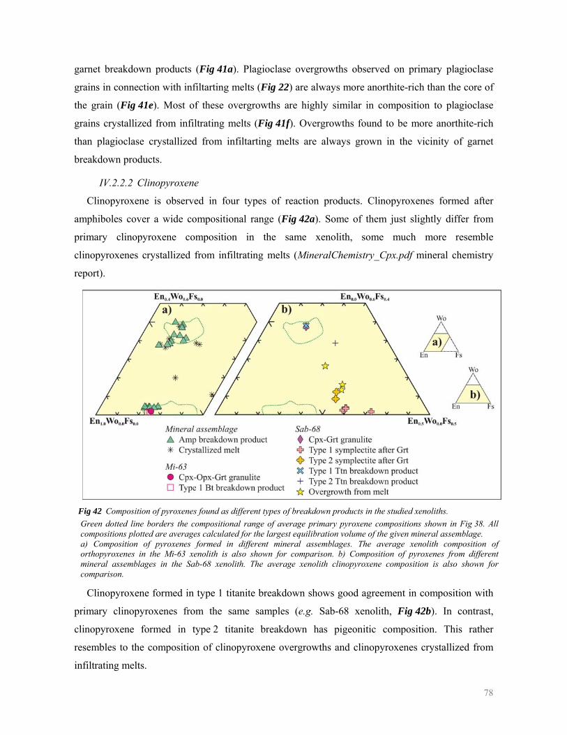
78
garnet breakdown products (Fig 41a). Plagioclase overgrowths observed on primary plagioclase
grains in connection with infiltarting melts (Fig 22) are always more anorthite-rich than the core of
the grain (Fig 41e). Most of these overgrowths are highly similar in composition to plagioclase
grains crystallized from infiltrating melts (Fig 41f). Overgrowths found to be more anorthite-rich
than plagioclase crystallized from infiltarting melts are always grown in the vicinity of garnet
breakdown products.
IV.2.2.2 Clinopyroxene
Clinopyroxene is observed in four types of reaction products. Clinopyroxenes formed after
amphiboles cover a wide compositional range (Fig 42a). Some of them just slightly differ from
primary clinopyroxene composition in the same xenolith, some much more resemble
clinopyroxenes crystallized from infiltrating melts (MineralChemistry_Cpx.pdf mineral chemistry
report).
Fig 42 Composition of pyroxenes found as different types of breakdown products in the studied xenoliths. Green dotted line borders the compositional range of average primary pyroxene compositions shown in Fig 38. All compositions plotted are averages calculated for the largest equilibration volume of the given mineral assemblage. a) Composition of pyroxenes formed in different mineral assemblages. The average xenolith composition of orthopyroxenes in the Mi-63 xenolith is also shown for comparison. b) Composition of pyroxenes from different mineral assemblages in the Sab-68 xenolith. The average xenolith clinopyroxene composition is also shown for comparison.
Clinopyroxene formed in type 1 titanite breakdown shows good agreement in composition with
primary clinopyroxenes from the same samples (e.g. Sab-68 xenolith, Fig 42b). In contrast,
clinopyroxene formed in type 2 titanite breakdown has pigeonitic composition. This rather
resembles to the composition of clinopyroxene overgrowths and clinopyroxenes crystallized from
infiltrating melts.
79
IV.2.2.3 Orthopyroxene
Orthopyroxene is formed in both types of garnet breakdown and in biotite breakdown.
Orthopyroxenes from type 1 symplectites (mg# = 0.27–0.60, 1.97–16.92 wt% Al2O3) are usually
more Fe- and Al-rich than primary orthopyroxenes (mg# = 0.54–0.77, 1.38–4.77 wt% Al2O3,
Fig 42b). Sometimes the Al-content of these orthopyroxenes decreases from the core towards the
rim (see the MineralChemistry_Opx.pdf mineral chemistry report). Pyroxenes found in type 2
symplectites (4.36–9.55 wt% Al2O3) are also more Al-rich than primary orthopyroxenes, but they
contain more Ca than orthopyroxenes formed in type 1 symplectites (e.g. in Sab-68 xenolith,
Fig 42b). In contrast, orthopyroxenes formed in biotite breakdown are Mg-rich and correspond to
the composition of primary orthopyroxene in the same xenolith (Fig 42b). Orthopyroxenes found in
amphibole breakdown products (mg# = 0.54–0.77, 1.72–2.18 wt% CaO) are also Mg-rich and
contain slightly more Ca than primary orthopyroxenes (0.44–1.46 wt% CaO).
IV.2.2.4 Amphibole
Amphiboles are formed in two types of reactions in the studied xenolith: amphibole
metasomatism of clinopyroxenes and melting of amphiboles. Although metasomatic amphiboles in
some samples can clearly be distinguished on the basis of petrography (Fig 24), they do not differ
from other amphiboles on the basis of main elements. However, their F-content may be different.
The highest F-content (0.15 p.f.u) was measured from the Mi-63 xenolith, where amphibole is
clearly metasomatic based on petrography. No systematic change in F-content was detected in the
other samples. Further study of amphibole genetics requires systematic measurements of minor and
trace elements as well. This is out of the scope of the present work. New amphiboles formed from
the melting of primary amphiboles have very variable composition (see the
MineralChemistry_Amp.pdf mineral chemistry report). Amphiboles formed in closed system
melting of primary amphiboles (Fig 25c) in A-11 xenolith contain much less TiO2 than the
precursor amphibole relics (1.55–2.10 wt% instead of 3.33–5.46 wt%). However, amphibole
overgrowths in connection with infiltrating melts (Fig 25d) are much more Ti-rich than amphibole
cores. For example, in A-16 xenolith primary amphiboles contains 3.08–3.43 wt% TiO2, while
overgrowths on primary amphiboles are of kaersutitic composition (4.07–5.48 wt% TiO2).
IV.2.2.5 Olivine
Olivines are found in three types of mineral assemblages: amphibole breakdown products,
type 2 symplectites after garnet and crystallized host melt within the xenoliths. All measured
olivines are pure forsterite–fayalite solid solutions, other minor components are negligible (see the
MineralChemistry_Ol.pdf mineral chemistry report, attached electronically). The composition of
80
different grains varies in a wide range. Olivines from crystallized melts are the most Mg-rich
(mg# = 0.63–0.81). Mg-content decreases from the core to the rim in some of these grains. Olivines
in amphibole breakdown products are restricted to a narrow range in mg# (0.62–0.64). This partly
overlaps both with olivines from crystallized host melt and olivines in type 2 symplectites after
garnet. Olivines from the latter mineral assemblage is quite consistent within a xenolith but
significatly varies between different samples (mg# = 0.28–0.66).
IV.2.2.6 Spinel
Spinel occurs most frequently in garnet breakdown products, but it was also observed in
crystallized melts within the xenoliths. Sometimes it is found as overgrowth on pyroxenes, and in
one case it appeared in the breakdown products of amphibole next to a symplectite after garnet. All
spinels are hercynite (34.6–80.6 mole%) and spinel ss. (17.7–60.8 mole%) solid solutions with
some magnetite (0.0–25.5 mole%), and minor ulvospinel (0.0–1.1 mole%), jacobsite (0.0–
1.5 mole%) and chromite (0.0–0.4 mole%) content (see analyses in the MineralChemistry_Spl.pdf
mineral chemistry report), no systematic relation with their occurrence was observed.
IV.2.2.7 Magnetite
Magnetite is found in the xenoliths as ilmenite–titanomagnetite intergrowths, as overgrowths on
Fe–Ti-oxides, as breakdown product of amphibole melting and in infiltrated melts crystallized
within the xenoliths. All analyses are found in the MineralChemistry_Mag.pdf mineral chemistry
report. Magnetite content was calculated according to Stormer (1983). The mineral chemistry of
magnetites appearing as ilmenite–titanomagnetite intergrowths or as overgrowths on Fe–Ti-oxides
is described in Section VII. All magnetites are magnetite–titanomagnetite solid solutions with some
spinel content. Magnetite composition varies in a wide range within the xenoliths, and the
compositional ranges of magnetites from amphibole melting products (30–78 mole% Mag) and
from crystallized melts (32–90 mole% Mag) totally overlap.
IV.2.2.8 Ilmenite
Ilmenite as a reaction product appears in Cpx–Ilm–Pl symplectites after titanite and as lamellae
ilmenite–titanomagnetite intergrowths. Ilmenites in the first mineral assemblage are nearly pure
ilmenites with minor hematite content (92.5–99.6 mole% Ilm). Ilmenite composition is uniform
within a sample, only small intersample variations were observed. The mineral chemistry of
ilmenites appearing as ilmenite–titanomagnetite intergrowths is described in Section VII.
81
IV.3 Mineral parageneses in the studied samples
Combining petrographical observations and mineral chemistry, different mineral parageneses
were identified in the xenoliths and their relative formation sequence was determined. Primary
mineral assemblages are the oldest preserved mineral parageneses in the studied xenoliths. Other
mineral parageneses are produced by the destabilization of the primary mineral assemblage during
the metamorphic evolution. The mineral chemistry of main rock-forming minerals in the primary
mineral assemblage show strong correlation within a xenolith, and different types of younger
mineral assemblages are found in samples with different chemistry. For this reason the xenoliths
are classified to five xenolith types: ordinary granulites, Ca-rich granulites, Mg-rich granulites, low
Ca rocks and Fe-rich granulites. The basis of xenolith type classification is given by compositional
groups of garnet (see Fig 34 in Section IV.2.1.1 for details). If the boundary between garnet
compositional groups is not easy to define or the xenolith is not uniform for this xenolith zone
property, additional xenolith zone properties, like the Ti-mineral paragenesis, are also taken into
account during the classification. The list of xenoliths and their types are found in Appendix 4 and
in the petrography report (Petrography.pdf).
Ordinary granulites all belong to the garnet compositional group I (Fig 34). They are basically
Cpx–Opx–Grt granulites or Cpx–Grt granulites which may contain amphibole and/or scapolite.
Garnets have intermediate grossular-content and magnesium number, which is correlated with
pyroxenes of intermediate magnesium number (Fig 38e). Garnet-free pyroxenite, Cpx–Pl fels and
Grt–Pl fels also occur in these xenoliths as bands, but the mineral chemistry of main rock-forming
minerals in the bands and in the adjacent granulite xenolith zones are the same. Regarding Ti-
minerals, Ilm–Tmt type and Rt-type mineral parageneses are observed in these samples. Garnet
breakdown, amphibole metasomatism, amphibole breakdown, scapolite breakdown and all
reactions of Fe–Ti oxides occur in this xenolith type. The reactions of Fe–Ti oxides record several
moments of lower crustal evolution as well as processes during xenolith – host melt interaction.
Many of these processes result in submicron scale changes of mineral chemistry and the relations of
different reactions is very complex. For this reason, reactions of Fe–Ti oxides are discussed
together with the results of high resolution electron beam microanalyses in Section VII.
Type 1 garnet breakdown products are found in all ordinary granulites, while the occurrence of
type 2 garnet breakdown products is always related to the presence of infiltrating melts (Fig 21b).
Mineral chemistry of plagioclase (Section IV.2.2.1), orthopyroxene (Section IV.2.2.3) and spinel
(Section IV.2.2.6) in the two types of garnet breakdown products are very similar. In addition,
olivine-bearing (type 2) garnet breakdown products always obliterate type 1 symplectites. These,
82
together with olivine mineral chemistry (Section IV.2.2.5) suggest that type 1 symplectites were
formed in the lower crust and type 2 garnet breakdown is the result of a chemical interaction
between type 1 garnet breakdown products and infiltrating host melts during xenolith – host melt
interaction. Further description and analysis of type 1 garnet breakdown is found in Section VI.
In some samples amphibole metasomatism can be identified on the basis of petrography
(Fig 24). However, the main element chemistry of primary and metasomatic amphiboles is not
different. In addition, the two types of amphiboles show the same amphibole breakdown reactions.
This suggests that metasomatic amphiboles were formed in a relatively early stage of metamorphic
evolution shortly after peak metamorphic conditions have changed. In contrast, amphibole
breakdown reactions all seem to be late events. Infiltrated host melt is clearly involved in the
breakdown reaction in most cases (Fig 25a–b, f). Olivine-bearing breakdown products always form
in this way. On the other hand, there is no evidence that closed sytem melting of amphibole
(Fig 25c) is the result of xenolith – host melt interaction. It could take place prior to the xenolith –
host melt interaction, but the presence of melt in the reaction products implies that this process is
also a late event. In case of scapolite breakdown, the interaction with infiltrating host melt clearly
obliterates the plagioclase corona formed in the reaction (Fig 26b). At the same time, the spongy
microstructure of the scapolite breakdown products is not expected to be stable for a long time at
lower crustal conditions. This suggests that the reaction took place at the late stage of metamorphic
evolution.
All samples containing Ca-rich garnets belong to Ca-rich granulites. This includes xenoliths
from garnet compositional groups II and VI (Fig 34), because xenoliths containing Fe-rich garnets
(group VI) cannot be distinguished from xenoliths with garnets of similar grossular-content
(group II) on the basis of plagioclase (Fig 36f) or pyroxene (Fig 38e) mineral chemistry or any
other xenolith zone properties. In addition, the Sab-38 xenolith with the most Ca-rich garnet
composition in garnet compositional group I was also classified to this group because of the similar
primary mineralogy and mineral reactions observed in the sample.
Ca-rich granulites are dominated by Cpx–Grt granulites, but pyroxenites and a Cpx–Opx–Grt
granulite also occur in this xenolith type. Amphibole may be found as hydrous phase, and all Ti-
mineral parageneses are observed. Garnet breakdown, amphibole metasomatism, amphibole
breakdown, reactions of Fe–Ti oxides and titanite breakdown are the mineral reactions of these
xenoliths. Microstructural and mineral chemical characteristics of the first four reaction types are
similar to those observed in ordinary granulites. One significant difference is that garnet breakdown
does nor occur or it has very limited extent in the Grt-bearing pyroxenite samples.
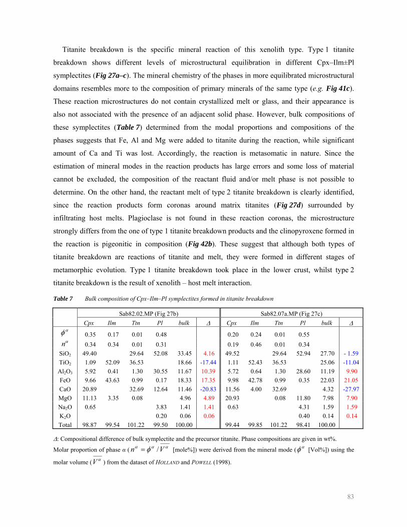
83
Titanite breakdown is the specific mineral reaction of this xenolith type. Type 1 titanite
breakdown shows different levels of microstructural equilibration in different Cpx–Ilm±Pl
symplectites (Fig 27a–c). The mineral chemistry of the phases in more equilibrated microstructural
domains resembles more to the composition of primary minerals of the same type (e.g. Fig 41c).
These reaction microstructures do not contain crystallized melt or glass, and their appearance is
also not associated with the presence of an adjacent solid phase. However, bulk compositions of
these symplectites (Table 7) determined from the modal proportions and compositions of the
phases suggests that Fe, Al and Mg were added to titanite during the reaction, while significant
amount of Ca and Ti was lost. Accordingly, the reaction is metasomatic in nature. Since the
estimation of mineral modes in the reaction products has large errors and some loss of material
cannot be excluded, the composition of the reactant fluid and/or melt phase is not possible to
determine. On the other hand, the reactant melt of type 2 titanite breakdown is clearly identified,
since the reaction products form coronas around matrix titanites (Fig 27d) surrounded by
infiltrating host melts. Plagioclase is not found in these reaction coronas, the microstructure
strongly differs from the one of type 1 titanite breakdown products and the clinopyroxene formed in
the reaction is pigeonitic in composition (Fig 42b). These suggest that although both types of
titanite breakdown are reactions of titanite and melt, they were formed in different stages of
metamorphic evolution. Type 1 titanite breakdown took place in the lower crust, whilst type 2
titanite breakdown is the result of xenolith – host melt interaction.
Table 7 Bulk composition of Cpx–Ilm–Pl symplectites formed in titanite breakdown
Sab82.02.MP (Fig 27b) Sab82.07a.MP (Fig 27c) Cpx Ilm Ttn Pl bulk Δ Cpx Ilm Ttn Pl bulk Δ αφ 0.35 0.17 0.01 0.48 0.20 0.24 0.01 0.55 αn 0.34 0.34 0.01 0.31 0.19 0.46 0.01 0.34
SiO2 49.40 29.64 52.08 33.45 4.16 49.52 29.64 52.94 27.70 - 1.59 TiO2 1.09 52.09 36.53 18.66 -17.44 1.11 52.43 36.53 25.06 -11.04 Al2O3 5.92 0.41 1.30 30.55 11.67 10.39 5.72 0.64 1.30 28.60 11.19 9.90 FeO 9.66 43.63 0.99 0.17 18.33 17.35 9.98 42.78 0.99 0.35 22.03 21.05 CaO 20.89 32.69 12.64 11.46 -20.83 11.56 4.00 32.69 4.32 -27.97 MgO 11.13 3.35 0.08 4.96 4.89 20.93 0.08 11.80 7.98 7.90 Na2O 0.65 3.83 1.41 1.41 0.63 4.31 1.59 1.59 K2O 0.20 0.06 0.06 0.40 0.14 0.14 Total 98.87 99.54 101.22 99.50 100.00 99.44 99.85 101.22 98.41 100.00
Δ: Compositional difference of bulk symplectite and the precursor titanite. Phase compositions are given in wt%.
Molar proportion of phase α ( ααα φ Vn /= [mole%]) were derived from the mineral mode ( αφ [Vol%]) using the
molar volume ( αV ) from the dataset of HOLLAND and POWELL (1998).
84
The garnet compositional groups III correspond to Mg-rich granulites. All Mg-rich granulites
are Cpx–Opx–Grt granulites, where the Mg-content of all Mg-bearing phases is the highest in the
studied xenoliths (mg#Grt = 0.58–0.62, Fig 34b; mg#Cpx = 0.76–0.82, mg#Opx = 0.73–0.77, Fig 38e;
mg#Bt = 0.76–0.83, Fig 40c–d; mg#Amp = 0.71–0.80, Fig 39a). Biotite appears as primary hydrous
phase in Mg-rich granulites and amphibole seems to be metasomatic on the basis of petrography
(Fig 24d). Besides amphibole metasomatism, type 1 garnet breakdown, amphibole breakdown and
both types of biotite breakdown are observed. The first three processes appear similarly as in
ordinary granulites. Amphibole metasomatism and garnet breakdown are assigned to the early stage
of metamorphic evolution while amphibole breakdown is related to xenolith – host melt interaction.
Type 1 biotite breakdown appears in the Mi-63 xenolith (Fig 23b). All reaction products are
crystallized and they are enclosed in primary garnet, which suggest that the reaction took place at
the very early stage of metamorphic evolution, probably during the formation of the primary
mineral assemblage. In contrast, type 2 biotite breakdown products contain significant amount of
melt and they form coronas around primary biotites. This implies that the process is a late event,
but similarly to closed system melting of amphibole, its relation to the xenolith – host melt
interaction cannot be determined on the basis of petrography and mineral chemistry.
Three strongly heterogeneous xenoliths from garnet compositional group IV (Fig 34) were
classified to the low Ca rock xenolith type: Mi-10, Mi-19 and Mi-75. Although the Mi-10 xenolith
(Fig 13b) is not uniform for garnet composition (Fig 30), regarding the striking similarities to
Mi-19 xenolith (Fig 31b), it was classified to this xenolith type. Low Ca rocks are built up by Opx–
Grt granulite, Pl–Grt fels and Cpx–Opx–Grt granulite xenolith zones which differ from each other
in chemistry even within one xenolith. Common chemical features are the low Ca-content of garnet
and plagioclase and the lack of clinopyroxene. Biotite is the primary hydrous phase and Rt-type Ti-
mineral paragenesis occurs in all samples of this xenolith type. The diffuse zoning of large, non-
equilibrium garnets in the Opx–Grt granulite xenolith zone of the Mi-10 xenolith (Fig 30) in
between Pl–Grt fels and Cpx–Opx–Grt granulite xenolith zones together with the continuous
increase of Ca-content of garnet (Fig 33a), plagioclase (Fig 36a) and orthopyroxene (Fig 38f) from
the Pl–Grt fels to the Cpx–Opx–Grt granulite suggest that the non-equilibrium Opx–Grt granulite
xenolith zone is a reaction product at the contact of Pl–Grt fels and Cpx–Opx–Grt granulite.
Regarding the well developed microstructure and grain size in the reaction zone, its formation may
have taken place at the early stage of metamorphic history. Although the complete transition from
Pl–Grt fels to Cpx–Opx–Grt granulite cannot be seen in the other two xenoliths, the microstructure
and similar mineral chemical trends (Fig 33a, Fig 36a) imply that the Opx–Grt granulite xenolith
zones of these xenoliths formed in a similar reaction as in the Mi-10 xenolith. Besides this reaction,
85
both types of biotite breakdown and type 1 garnet breakdown is observed in the rock. Biotite relics
associated with CO2-rich fluid inclusions (Fig 23a, Török et al. 2007) are enclosed in large, non-
equilibrium garnets and orthopyroxenes interpreted to be reaction products of the two different rock
types. This suggests that the melting of biotite was associated with the formation of Opx–Grt
granulite xenolith zones. Type 1 symplectites after garnet consume all garnets in low Ca rocks,
even the reaction products in Opx–Grt granulite xenolith zones (Fig 16f, Fig 30b). This suggests
that garnet breakdown took place in a later stage of metamorphic evolution. Besides these
reactions, type 2 breakdown of biotite (Fig 23c–d) is also observed in the rock. The presence of
melt in the reaction products implies that biotite melting is a late stage reaction as in Mg-rich
granulites.
Fe-rich granulites correspond to the garnet compositional group V (Fig 34). Garnets have
intermediate grossular content as in ordinary granulites, but garnet (mg#Grt = 0.32, Fig 34b) as well
as clinopyroxene (mg#Cpx = 0.57–0.64, Fig 38e) is significantly more Fe-rich than in ordinary
granulites (mg#Grt = 0.36–0.54, Fig 34b; mg#Cpx = 0.59–0.77, Fig 38e). All xenoliths classified to
this xenolith type are Cpx–Grt granulites which contain ilmenites as primary Ti-minerals.
Amphibole occurs as inclusion in the A-11 xenolith. Type 1 garnet breakdown and type 1
titanomagnetite lamellae in ilmenite are observed as reaction products in these xenoliths. The
microstructure and mineral chemistry of these reaction products corresponds to the similar reaction
microstructures in ordinary granulites.
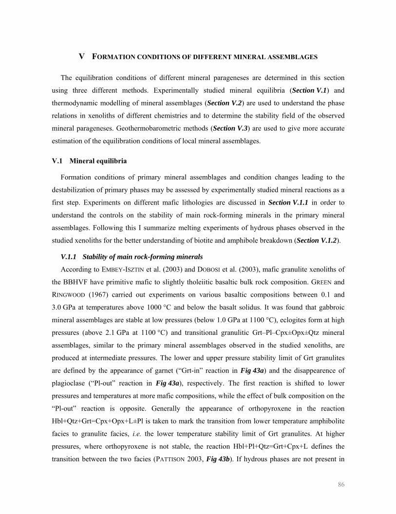
86
V FORMATION CONDITIONS OF DIFFERENT MINERAL ASSEMBLAGES
The equilibration conditions of different mineral parageneses are determined in this section
using three different methods. Experimentally studied mineral equilibria (Section V.1) and
thermodynamic modelling of mineral assemblages (Section V.2) are used to understand the phase
relations in xenoliths of different chemistries and to determine the stability field of the observed
mineral parageneses. Geothermobarometric methods (Section V.3) are used to give more accurate
estimation of the equilibration conditions of local mineral assemblages.
V.1 Mineral equilibria
Formation conditions of primary mineral assemblages and condition changes leading to the
destabilization of primary phases may be assessed by experimentally studied mineral reactions as a
first step. Experiments on different mafic lithologies are discussed in Section V.1.1 in order to
understand the controls on the stability of main rock-forming minerals in the primary mineral
assemblages. Following this I summarize melting experiments of hydrous phases observed in the
studied xenoliths for the better understanding of biotite and amphibole breakdown (Section V.1.2).
V.1.1 Stability of main rock-forming minerals
According to EMBEY-ISZTIN et al. (2003) and DOBOSI et al. (2003), mafic granulite xenoliths of
the BBHVF have primitive mafic to slightly tholeiitic basaltic bulk rock composition. GREEN and
RINGWOOD (1967) carried out experiments on various basaltic compositions between 0.1 and
3.0 GPa at temperatures above 1000 °C and below the basalt solidus. It was found that gabbroic
mineral assemblages are stable at low pressures (below 1.0 GPa at 1100 °C), eclogites form at high
pressures (above 2.1 GPa at 1100 °C) and transitional granulitic Grt–Pl–Cpx±Opx±Qtz mineral
assemblages, similar to the primary mineral assemblages observed in the studied xenoliths, are
produced at intermediate pressures. The lower and upper pressure stability limit of Grt granulites
are defined by the appearance of garnet (“Grt-in” reaction in Fig 43a) and the disappearence of
plagioclase (“Pl-out” reaction in Fig 43a), respectively. The first reaction is shifted to lower
pressures and temperatures at more mafic compositions, while the effect of bulk composition on the
“Pl-out” reaction is opposite. Generally the appearance of orthopyroxene in the reaction
Hbl+Qtz+Grt=Cpx+Opx+L±Pl is taken to mark the transition from lower temperature amphibolite
facies to granulite facies, i.e. the lower temperature stability limit of Grt granulites. At higher
pressures, where orthopyroxene is not stable, the reaction Hbl+Pl+Qtz=Grt+Cpx+L defines the
transition between the two facies (PATTISON 2003, Fig 43b). If hydrous phases are not present in
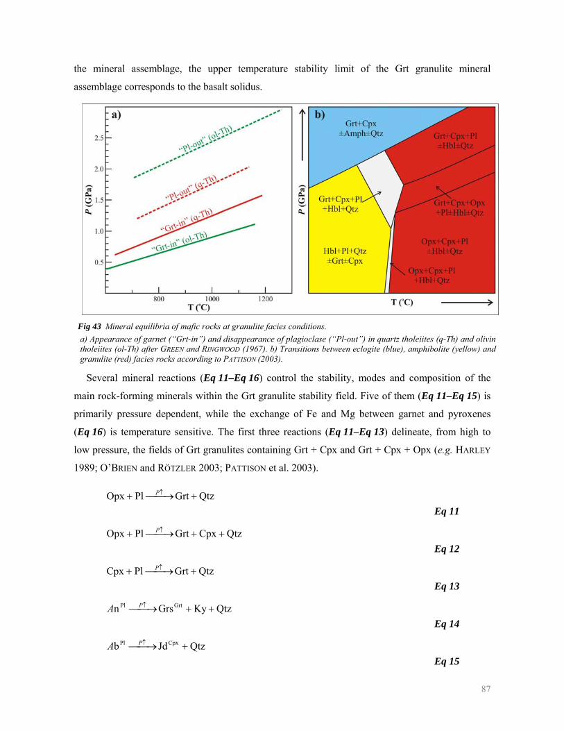
87
the mineral assemblage, the upper temperature stability limit of the Grt granulite mineral
assemblage corresponds to the basalt solidus.
Fig 43 Mineral equilibria of mafic rocks at granulite facies conditions. a) Appearance of garnet (“Grt-in”) and disappearance of plagioclase (“Pl-out”) in quartz tholeiites (q-Th) and olivin tholeiites (ol-Th) after GREEN and RINGWOOD (1967). b) Transitions between eclogite (blue), amphibolite (yellow) and granulite (red) facies rocks according to PATTISON (2003).
Several mineral reactions (Eq 11–Eq 16) control the stability, modes and composition of the
main rock-forming minerals within the Grt granulite stability field. Five of them (Eq 11–Eq 15) is
primarily pressure dependent, while the exchange of Fe and Mg between garnet and pyroxenes
(Eq 16) is temperature sensitive. The first three reactions (Eq 11–Eq 13) delineate, from high to
low pressure, the fields of Grt granulites containing Grt + Cpx and Grt + Cpx + Opx (e.g. HARLEY
1989; O’BRIEN and RÖTZLER 2003; PATTISON et al. 2003).
QtzGrtPlOpx +⎯→⎯+ ↑P Eq 11
QtzCpxGrtPlOpx ++⎯→⎯+ ↑P Eq 12
QtzGrtPlCpx +⎯→⎯+ ↑P Eq 13
QtzKyGrsn GrtPl ++⎯→⎯ ↑PA Eq 14
QtzJdb CpxPl +⎯→⎯ ↑PA Eq 15
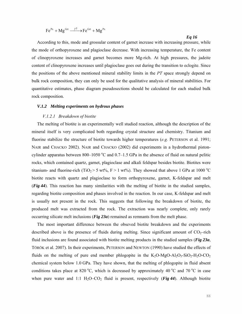
88
PxGrtGrtPx MgFeMgFe +⎯→⎯+ ↑T Eq 16
According to this, mode and grossular content of garnet increase with increasing pressure, while
the mode of orthopyroxene and plagioclase decrease. With increasing temperature, the Fe content
of clinopyroxene increases and garnet becomes more Mg-rich. At high pressures, the jadeite
content of clinopyroxene increases until plagioclase goes out during the transition to eclogite. Since
the positions of the above mentioned mineral stability limits in the PT space strongly depend on
bulk rock composition, they can only be used for the qualitative analysis of mineral stabilities. For
quantitative estimates, phase diagram pseudosections should be calculated for each studied bulk
rock composition.
V.1.2 Melting experiments on hydrous phases
V.1.2.1 Breakdown of biotite
The melting of biotite is an experimentally well studied reaction, although the description of the
mineral itself is very complicated both regarding crystal structure and chemistry. Titanium and
fluorine stabilize the structure of biotite towards higher temperatures (e.g. PETERSON et al. 1991;
NAIR and CHACKO 2002). NAIR and CHACKO (2002) did experiments in a hydrothermal piston-
cylinder apparatus between 800–1050 oC and 0.7–1.5 GPa in the absence of fluid on natural pelitic
rocks, which contained quartz, garnet, plagioclase and alkali feldspar besides biotite. Biotites were
titanium- and fluorine-rich (TiO2 > 5 wt%, F > 1 wt%). They showed that above 1 GPa at 1000 oC
biotite reacts with quartz and plagioclase to form orthopyroxene, garnet, K-feldspar and melt
(Fig 44). This reaction has many similarities with the melting of biotite in the studied samples,
regarding biotite composition and phases involved in the reaction. In our case, K-feldspar and melt
is usually not present in the rock. This suggests that following the breakdown of biotite, the
produced melt was extracted from the rock. The extraction was nearly complete, only rarely
occurring silicate melt inclusions (Fig 23a) remained as remnants from the melt phase.
The most important difference between the obseved biotite breakdown and the experiments
described above is the presence of fluids during melting. Since significant amount of CO2–rich
fluid inclusions are found associated with biotite melting products in the studied samples (Fig 23a,
TÖRÖK et al. 2007). In their experiments, PETERSON and NEWTON (1990) have studied the effects of
fluids on the melting of pure end member phlogopite in the K2O-MgO-Al2O3-SiO2-H2O-CO2
chemical system below 1.0 GPa. They have shown, that the melting of phlogopite in fluid absent
conditions takes place at 820 oC, which is decreased by approximately 40 oC and 70 oC in case
when pure water and 1:1 H2O–CO2 fluid is present, respectively (Fig 44). Although biotite
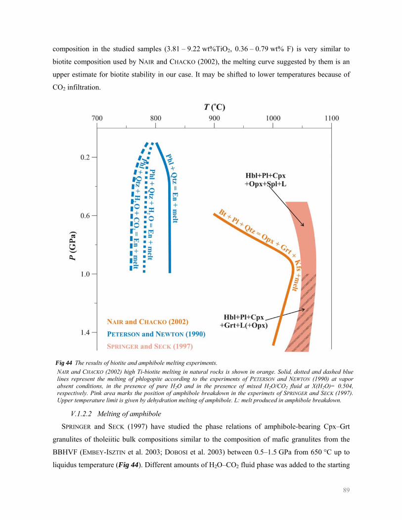
89
composition in the studied samples (3.81 – 9.22 wt%TiO2, 0.36 – 0.79 wt% F) is very similar to
biotite composition used by NAIR and CHACKO (2002), the melting curve suggested by them is an
upper estimate for biotite stability in our case. It may be shifted to lower temperatures because of
CO2 infiltration.
Fig 44 The results of biotite and amphibole melting experiments. NAIR and CHACKO (2002) high Ti-biotite melting in natural rocks is shown in orange. Solid, dotted and dashed blue lines represent the melting of phlogopite according to the experiments of PETERSON and NEWTON (1990) at vapor absent conditions, in the presence of pure H2O and in the presence of mixed H2O/CO2 fluid at X(H2O)= 0.504, respectively. Pink area marks the position of amphibole breakdown in the experimets of SPRINGER and SECK (1997). Upper temperature limit is given by dehydration melting of amphibole. L: melt produced in amphibole breakdown.
V.1.2.2 Melting of amphibole
SPRINGER and SECK (1997) have studied the phase relations of amphibole-bearing Cpx–Grt
granulites of tholeiitic bulk compositions similar to the composition of mafic granulites from the
BBHVF (EMBEY-ISZTIN et al. 2003; DOBOSI et al. 2003) between 0.5–1.5 GPa from 650 °C up to
liquidus temperature (Fig 44). Different amounts of H2O–CO2 fluid phase was added to the starting
90
material in different runs. They have found that amphibole reacts out between 1020–1050 °C. At
pressures below 1.0 GPa clinopyroxene, plagioclase, orthopyroxene spinel and melt is produced in
the reaction, while at higher pressures spinel is replaced by garnet in the reaction products. Slight
increase in the bulk fluid content did not effect the melting temperature, it rather increased the
mode of melt produced. In dehydration melting experiments, where no fluid phase was added to the
bulk rock, the amphibole out reaction shifted to somewhat higher temperatures (1075 °C at
1.5 GPa) and melt fraction was not observed at tempeartures below the amphibole breakdown
curve.
Amphibole breakdown products in the studied samples do not contain garnet. This suggests that
amphibole melting occurred below about 1.0 GPa (e.g. WYLLIE and WOLF 1993; SPRINGER and
SECK 1997). On the other hand, the melting point of amphiboles studied in the PhD thesis is
difficult to determine because many of them contain significant amount of Ti and F (up to 0.5 and
0.25 p.f.u., respectively). TSUNOGAE et al. (2003) have shown that the presence of 0.5 p.f.u.
fluorine in pargasitic amphibole increases the melting temperature with nearly 150 °C, but no
quantitative data are available for the studied amphibole compositions.
V.2 Thermodynamic modelling
In order to learn more about the stability limits of the observed mineral assemblages, different
types of phase diagrams are constructed using the PERPLEX software (CONNOLLY 1990) and the
database and solution models of HOLLAND and POWELL (1998). In this section I study the
behaviour of primary mineral assemblages with changing pressure and temperature. The
thermodynamic problem is defined first (Section V.2.1) then the calculated phase diagram
pseudosections are discussed (Section V.2.2). Further thermodynamic analysis of reaction
microstructures are found in Sections VI and VII.
V.2.1 Problem definition
The mineralogy, chemistry and mineral reactions observed in the studied samples are controlled
by three main variables: pressure, temperature and bulk composition. As a first approximation I
treat primary mineral assemblages as chemically closed systems and discuss their behaviour with
changing pressure and temperature using phase diagram pseudosections constructed for bulk
xenolith composition. Although a number of experiments have pointed out the crucial role of Ti
and F on the stability of hydrous phases (e.g. PETERSON et al. 1991; TSUNOGAE et al. 2003), their
thermodynamic treatment is not well-established yet. A solution model for biotite with high Ti-
content came out recently (e.g. TAJČMANOVÁ et al. 2009), but the effect of fluorine on biotite
91
stability is still not clarified. In case of amphibole, the treatment of high Ti-content is also a
problem (e.g. MASSONE and WILMER 2008). Since the result of thermodynamic modelling strongly
depends on the solution models used, samples containing hydrous phases were excluded from these
types of calculations. Scapolite-bearing samples were also excluded because scapolite solution
models (e.g. SOKOLOVA and HAWTHORNE 2008) are developed for carbonate end members.
However, scapolite in the studied xenoliths contain siginificant amount of sulphate
(MineralChemistry_Scp.pdf), and the role of sulfur in the system is not known at any precision.
Considering the measured compositions of the remaining primary phases, thermodynamic
modelling was done in the Na2O–CaO–FeO–MgO–Al2O3–SiO2–TiO2–O2 (NCFMASTO) chemical
system. To account for fine-grained reaction products and infiltrating host basalt in the xenoliths,
bulk rock compositions were derived from the modal proportions and chemical compositions of the
phases corrected by the molar volumes from the dataset of HOLLAND and POWELL (1998). Modal
analyses were done using the PolyLX toolbox of MATLAB developed by O. LEXA.
The five xenolith types distinguished on the basis of petrography and mineral chemistry defines
five basically different bulk rock compositions. Since the main petrographical and chemical
characteristics of the xenoliths within one xenolith type are the same, the phase relations of each
type can be described by the thermodynamic modelling of a representative sample. However,
chemically homogeneous xenoliths devoid of primary hydrous phase or scapolite and significant
chemical overprint from the host basalt occur only rarely. For this reason, the thermodynamic
modelling of Mg-rich and Fe-rich granulites was not possible. Ordinary granulites, Ca-rich
granulites and low Ca rocks are represented by the Sab-79, the Sab-32 xenoliths and a fine-grained,
chemically homogeneous part of the Mi-19 xenolith, respectively. Bulk rock compositions are
displayed on the calculated phase diagram pseudosections (Fig 45). Since the Fe3+ content of the
samples was not measured, oxygen was treated as a mobile component and calculations were done
using different oxygen buffers. In all cases the same solution models of garnet, plagioclase, olivine,
spinel (HOLLAND and POWELL 1998), clinopyroxene (HOLLAND and POWELL 1996), orthopyroxene
(POWELL and HOLLAND 1999), melt (WHITE et al. 2001), ilmenite and magnetite (WOOD et al.
1991) were used.
V.2.2 Phase diagram pseudosections of primary mineral assemblages
Phase diagram pseudosections for bulk rock composition of the selected xenoliths were
calculated between 0.1 MPa – 1.8 GPa and 700 – 1300 °C in order to see the behaviour of the given
xenolith type in all possible tectonic environments, as well as during the interaction with the host
basalt. The reviews HARLEY (1989), O’BRIEN and RÖTZLER (2003) and O’BRIEN (2008) reported
92
equilibration conditions between 0.9 – 1.8 GPa and 700 – 1100 °C for granulites from different
tectonic settings all over the world. 1.8 GPa is the maximum pressure estimated for the
overthickened orogenic root of the Himalayas (LIU and ZHONG 1997; DING and ZHONG 1999).
Extremely high temperature and low pressure conditions may be reached during the xenolith – host
melt interaction. According to the silicate melt inclusion studies of KÓTHAY et al. (2005), the
temperature of the alkali basaltic magma in the BBHVF was at least 1220 – 1270 °C.
Although in general all studied samples have mafic composition, pseudosections calculated for
the selected xenoliths strongly differ from each other. The stability fields of the observed primary
mineral assemblages (show in Fig 45) correspond to pressures above 1.0 GPa in all rock
chemistries. Although the mineral parageneses predicted by the phase diagram pseudosections
describe well the observed mineralogy, the chemical compositions and modes of the phases are not
in so good agreement. This may be caused by the uncertainties in determining the bulk rock
composition. For this reason, these types of phase diagrams can only be used to analyze
qualitatively processes induced by pressure or temperature changes at constant bulk chemistry.
The disappearance of garnet with decreasing pressure defining the lower pressure limit of the
Grt granulite field is found in all phase diagram pseudosections. However, the position of the
reaction strongly depends on the bulk rock composition. In the Mi-19 xenolith where the Ca/Fe
ratio is the smallest, garnet is stable at pressures corresponding to the present day lower crust
(>0.4 GPa at 1000 °C, Fig 45c). At the same time in the most aluminous sample (Sab-79, Fig 45a)
garnet appears above 0.8 GPa at the same temperature, which is suggested to be the pressure at
Moho depth beneath the Pannonian Basin (e.g. POSGAY et al. 1991). In general, the grossular
content of garnet decreases with decreasing pressure. This may explain the Ca-zoning in garnet
observed in the Mi-75 and Sab-59 xenoliths (Fig 29, Table 3). Although garnet breakdown with
decreasing pressure is seen in all phase diagram pseudosections, the Opx–Pl–Spl mineral
assemblage of type 1 symplectite after garnet does not correspond to the predicted low pressure
mineral assemblages. For this reason, the breakdown of garnet is studied in details in Section VI.
The plagioclase out reaction defining the upper pressure stability limit of Grt granulites is not
seen by ordinary granulites and low Ca rocks in the studied pressure range above 800 °C. In
contrast, plagioclase reacts out with increasing pressure relatively early in Ca-rich granulites
(1.2 GPa at 1000 °C, Fig 45b). This explains the low modal abundance of plagioclase in this
xenolith type. In this bulk chemistry, garnet pyroxenites are not indicating extremely high
pressures. The presence of orthopyroxene is the most sensitive for bulk rock composition. In low
Ca rocks it is stable nearly in the complete PT range (Fig 45c), while it does not appear in Ca-rich
granulites (Fig 45b).
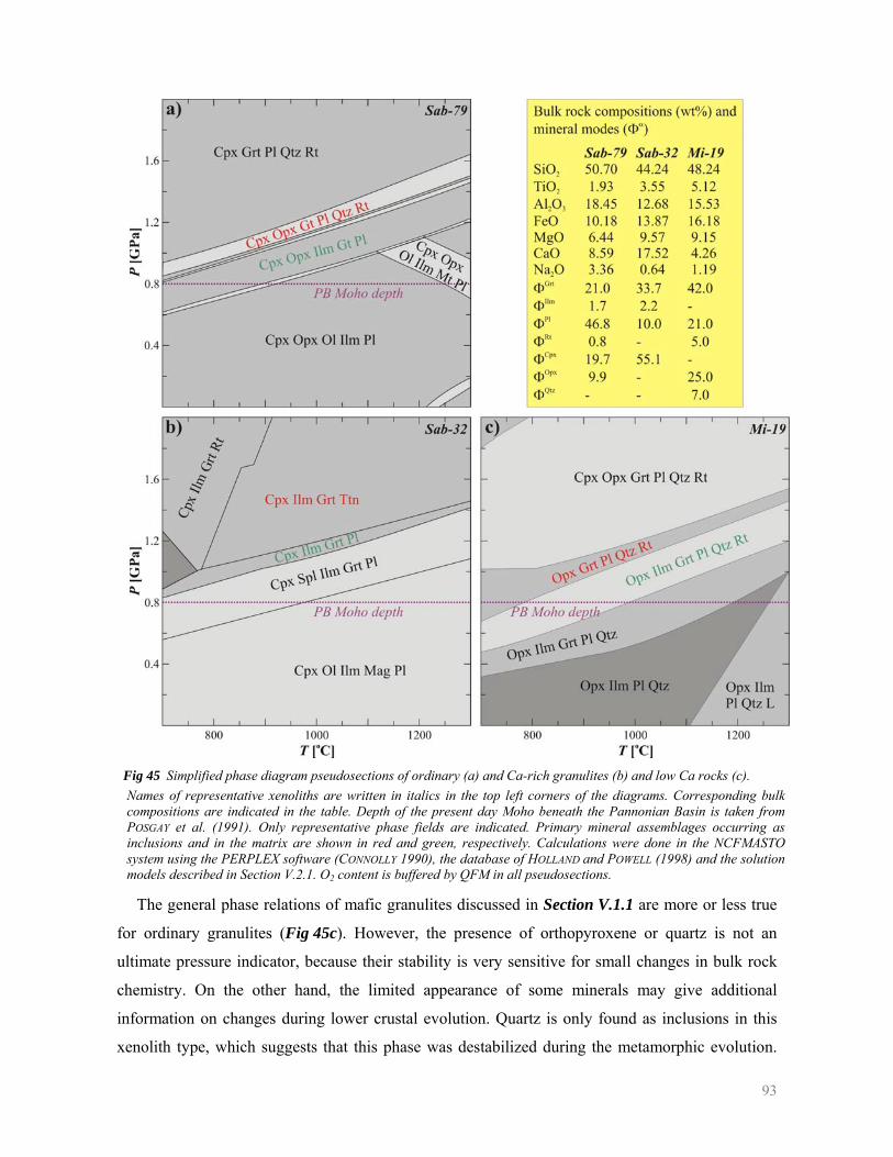
93
Fig 45 Simplified phase diagram pseudosections of ordinary (a) and Ca-rich granulites (b) and low Ca rocks (c). Names of representative xenoliths are written in italics in the top left corners of the diagrams. Corresponding bulk compositions are indicated in the table. Depth of the present day Moho beneath the Pannonian Basin is taken from POSGAY et al. (1991). Only representative phase fields are indicated. Primary mineral assemblages occurring as inclusions and in the matrix are shown in red and green, respectively. Calculations were done in the NCFMASTO system using the PERPLEX software (CONNOLLY 1990), the database of HOLLAND and POWELL (1998) and the solution models described in Section V.2.1. O2 content is buffered by QFM in all pseudosections.
The general phase relations of mafic granulites discussed in Section V.1.1 are more or less true
for ordinary granulites (Fig 45c). However, the presence of orthopyroxene or quartz is not an
ultimate pressure indicator, because their stability is very sensitive for small changes in bulk rock
chemistry. On the other hand, the limited appearance of some minerals may give additional
information on changes during lower crustal evolution. Quartz is only found as inclusions in this
xenolith type, which suggests that this phase was destabilized during the metamorphic evolution.
94
On the basis of the calculated pseudosections decreasing pressure and/or increasing temperature
can result in this process. Titanite relics in Ca-rich granulites also indicate high formation pressures
and titanite reacts out with decreasing pressure in a similar way as quartz at constant bulk rock
chemistry. However, from the bulk compositions calculated for Cpx–Ilm–Pl symplectites formed in
type 1 titanite breakdown (Table 7) this reaction is clearly metasomatic in nature.
Rutile is also observed as inclusions in the main rock-forming mineral phases in ordinary
granulites with Rt-type Ti-mineral parageneses, while ilmenite is present in the matrix (Fig 15c–d).
The transformation of Rt-bearing granulites to Ilm-bearing ones has slope similar to the quartz out
reaction. However, this reaction is very sensitive for oxygen fugacity, because Fe3+ stabilizes
ilmenite towards higher pressure. For this reason, the appearance of ilmenite in the matrix can be
the result of PT changes and a metasomatic event, as well. In case of magnetite, oxygen fugacity is
the main control on its stability. Detailed thermodynamic analysis of the reactions of Fe–Ti oxides
is found in Section VII.
V.3 Geothermobarometry
Experimentally determined mineral equilibria and thermodynamic analysis of the studied
xenoliths give only qualitative information on the formation conditions of different mineral
assemblages. For the quantification the equilibration pressure and temperature,
geothermobarometry needs to be done. After the selection of adequate mineral compositions from
true equilibrium mineral assemblages (Section V.3.1), I estimated and compared the temperature of
equilibration for different mineral pairs according to different methods (Section V.3.2). I selected
the thermometers best applicable for the studied rocks and these temperatures were used for
pressure estimation in Section V.3.3. Finally, equilibration PT conditions of the primary mineral
assemblages were used up to construct a paleogeotherm (Section V.3.4).
V.3.1 Construction of the dataset for geothermobarometry
Six type of mineral assemblages were the subject of geothermobarometric analysis. Temperature
was estimated using Grt–Cpx, Grt–Opx and Cpx–Opx mineral pairs, while Grt–Cpx–Pl, Grt–Opx–
Pl and Cpx–Pl mineral assemblages were used for barometry. Pressure and temperature estimations
were done in MS Excel worksheets designed for the comparison of different geothermobarometric
methods for a given mineral assemblage on large datasets. Input data for the calculations were
prepared by using the GTB Queries in the GRANULITE database (Section III.3.3). In all cases the
state of equilibrium was carefully checked.
95
If the requirements of chemical equilibrium are regarded strictly only mineral assemblages
containing the given ’mineral pair’ as adjacent grains, referred to as local mineral assemblages, can
be used for geothermobarometry. However, if mineral composition is uniform within a larger
equilibration volume, much higher number of ’mineral pair’ combinations are allowed. Since the
uncertainty of pressure or temperature estimation can be reduced by increasing the number of
different mineral assemblages used for thermobarometry, the dataset is evaluated according to both
equilibrium requirements. In both cases, adequate average grain compositions are used. Analyses
are averaged in different ways depending on the zonation type of the grain (Fig 12). Grains
showing diffuse or complex zoning are excluded from the geothermobarometric analysis as a first
approximation. Average grain composition is calculated for homogeneous grains, while averages
for core and zone compositions are calculated separately in grains with growth zoning. The
averaging type of each microprobe analysis is stored as an average position in the GRANULITE
database. Grains are combined to the same mineral assemblage by the database only if analyses are
available from the same average position and geothermobarometry is done for different average
positions separately. In case of local mineral assemblages, ’mineral pairs’ correspond to grains
within the same local mineral assemblage. In samples which are chemically homogeneous at
xenolith zone or xenolith level, ’mineral pairs’ are generated from grains within the same
equilibration volume. Average zone compositions are excluded from these types of
geothermobarometric calculations. If it is possible, the state of equilibrium in local mineral
assemblages is also verified by comparing element partition coefficients (KD values) calculated
from measured data to the ones predicted from solution models. An example of this comparison is
shown in Fig 46.
Datasets constructed in the GRANULITE database are exported to MS Excel spreadsheets
where geothermobarometric calculations are done. The results of these calculations are shown in
the following sections.
V.3.2 Thermometry
Temperature estimations were done for garnet–clinopyroxene, garnet–orthopyroxene and
clinopyroxene–orthopyroxene pairs. In all cases, more calibrations were compared. The results are
discussed for each mineral pair.
V.3.2.1 Grt–Cpx
Equilibration temperatures of primary mineral assemblages were estimated using four different
thermometers (ELLIS and GREEN 1979; KROGH 1988; PATTISON and NEWTON 1989 and AI 1994)
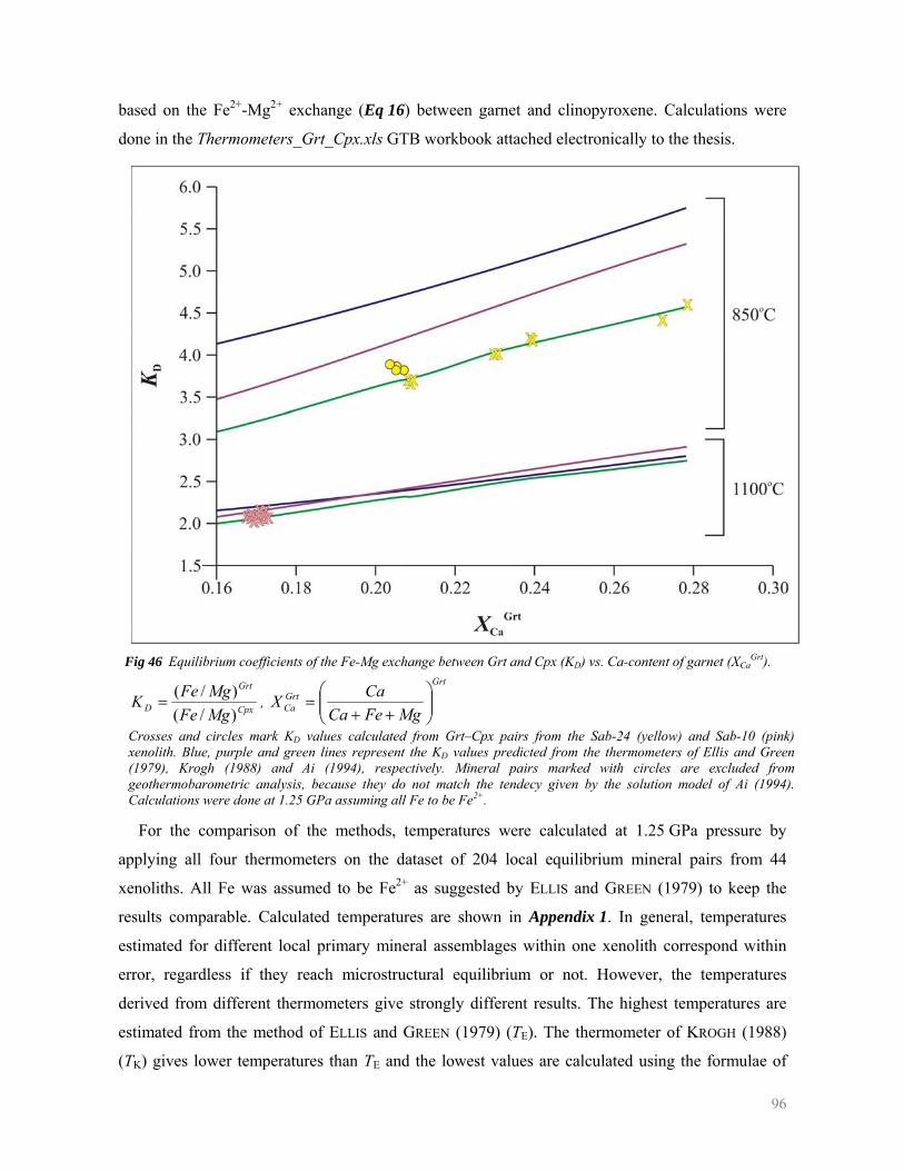
96
based on the Fe2+-Mg2+ exchange (Eq 16) between garnet and clinopyroxene. Calculations were
done in the Thermometers_Grt_Cpx.xls GTB workbook attached electronically to the thesis.
Fig 46 Equilibrium coefficients of the Fe-Mg exchange between Grt and Cpx (KD) vs. Ca-content of garnet (XCa
Grt).
Cpx
Grt
D MgFeMgFeK
)/()/(
= , Grt
GrtCa MgFeCa
CaX ⎟⎟⎠
⎞⎜⎜⎝
⎛++
=
Crosses and circles mark KD values calculated from Grt–Cpx pairs from the Sab-24 (yellow) and Sab-10 (pink) xenolith. Blue, purple and green lines represent the KD values predicted from the thermometers of Ellis and Green (1979), Krogh (1988) and Ai (1994), respectively. Mineral pairs marked with circles are excluded from geothermobarometric analysis, because they do not match the tendecy given by the solution model of Ai (1994). Calculations were done at 1.25 GPa assuming all Fe to be Fe2+.
For the comparison of the methods, temperatures were calculated at 1.25 GPa pressure by
applying all four thermometers on the dataset of 204 local equilibrium mineral pairs from 44
xenoliths. All Fe was assumed to be Fe2+ as suggested by ELLIS and GREEN (1979) to keep the
results comparable. Calculated temperatures are shown in Appendix 1. In general, temperatures
estimated for different local primary mineral assemblages within one xenolith correspond within
error, regardless if they reach microstructural equilibrium or not. However, the temperatures
derived from different thermometers give strongly different results. The highest temperatures are
estimated from the method of ELLIS and GREEN (1979) (TE). The thermometer of KROGH (1988)
(TK) gives lower temperatures than TE and the lowest values are calculated using the formulae of
97
PATTISON and NEWTON (1989) (TPN) and AI (1994) (TA). The difference between TE and TA reaches
100 °C in low temperature samples, and it reduces below 50 °C in high temperature samples. The
same trend is observable for TK, just the largest differences are around 60 °C. There is no systematic
difference between TPN and TA and they usually correspond within error. In order to find the
method which describes the studied dataset the best, equilibrium constants (KD) were calculated
from the ELLIS and GREEN (1979), the KROGH (1988) and the AI (1994) thermometers for selected
temperatures as a function of Ca-content in garnet. These data were compared to KD values
calculated from the studied samples (Fig 46). At high temperatures, all models reproduce the
dataset within error, but significant differences are found in case of low temperature samples,
where only the model of AI (1994) reproduces the partition coefficients calculated from the
samples. The formulation of the PATTISON and NEWTON (1989) thermometer does not allow for
such a comparison. In addition, the use of this method is very limited in the studied rocks because
in many samples the Ca content of garnet is out of the calibration range. For this reason,
temperatures estimated from the thermometer of AI (1994) were used for further calculations.
Although none of the thermometer formulations corrects for the Fe3+ content of the phases,
many authors (e.g. PATTISON and NEWTON 1989; AI 1994) suggest to take into consideration Fe3+
content in clinopyroxene when equilibrium constants are derived from natural rocks. Temperatures
estimated assuming all Fe to be Fe2+ as suggested by ELLIS and GREEN (1979) are upper estimates
and sometimes irrealistically high (up to 1200 °C, see Appendix 1). I applied the method of DROOP
(1987) to estimate the Fe3+ content in clinopyroxene and then compared TA temperatures corrected
and not corrected for Fe3+ (TAC and TA
NC, respectively, Fig 47). Since the Fe3+ content of
clinopyroxene strongly varies between and within the samples, the effect of correction is different.
In samples not containing significant amount of Fe3+ (e.g. Sab-122), the two temperatures agree
well. However, in the majority of the xenoliths, where Fe3+ content exceeds 0.05 p.f.u., both
temperatures have a slope as a function of Fe3+ content (Fig 47). This suggests that TANC
overestimates the temperature, while TAC underestimates it. In many cases both estimated
temperatures are linear functions of Fe3+ content within one sample, and TANC has negative, while
TAC has positive slope. If we extrapolate these temperatures to zero Fe3+ content they agree well
(Fig 47). In these cases, the average of extrapolated temperatures was accepted as equilibration
temperature. In the last group of xenoliths, these types of linear trends are not observable but the
difference between TAC and TA
NC may exceed 100 °C. For these samples the uncertainty of
temperature estimation is very high. For plotting TAC and TA
NC were averaged together and
maximum and minimum estimated temperatures were used as error bars. In case of the other
samples, the standard deviation of the used dataset was plotted as error. The estimated values are
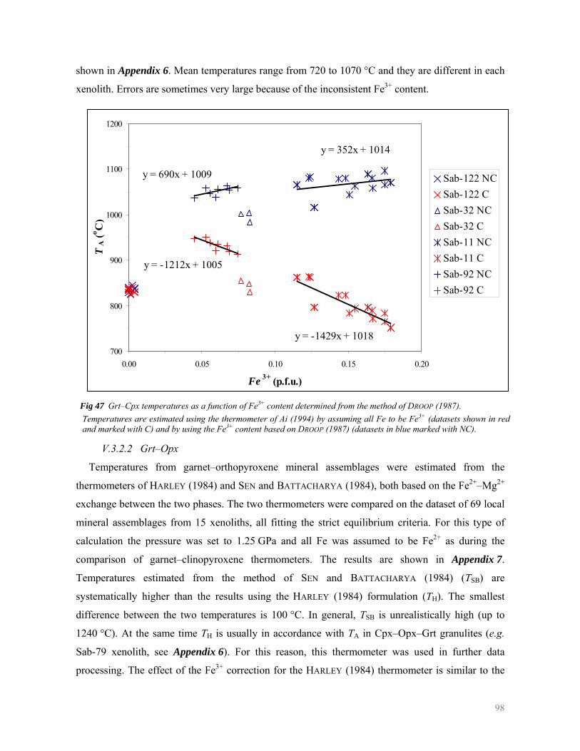
98
shown in Appendix 6. Mean temperatures range from 720 to 1070 °C and they are different in each
xenolith. Errors are sometimes very large because of the inconsistent Fe3+ content.
y = 352x + 1014
y = -1429x + 1018
y = 690x + 1009
y = -1212x + 1005
700
800
900
1000
1100
1200
0.00 0.05 0.10 0.15 0.20
Fe 3+ (p.f.u.)
TA (o C
)
Sab-122 NCSab-122 CSab-32 NCSab-32 CSab-11 NCSab-11 CSab-92 NCSab-92 C
Fig 47 Grt–Cpx temperatures as a function of Fe3+ content determined from the method of DROOP (1987). Temperatures are estimated using the thermometer of Ai (1994) by assuming all Fe to be Fe3+ (datasets shown in red and marked with C) and by using the Fe3+ content based on DROOP (1987) (datasets in blue marked with NC).
V.3.2.2 Grt–Opx
Temperatures from garnet–orthopyroxene mineral assemblages were estimated from the
thermometers of HARLEY (1984) and SEN and BATTACHARYA (1984), both based on the Fe2+–Mg2+
exchange between the two phases. The two thermometers were compared on the dataset of 69 local
mineral assemblages from 15 xenoliths, all fitting the strict equilibrium criteria. For this type of
calculation the pressure was set to 1.25 GPa and all Fe was assumed to be Fe2+ as during the
comparison of garnet–clinopyroxene thermometers. The results are shown in Appendix 7.
Temperatures estimated from the method of SEN and BATTACHARYA (1984) (TSB) are
systematically higher than the results using the HARLEY (1984) formulation (TH). The smallest
difference between the two temperatures is 100 °C. In general, TSB is unrealistically high (up to
1240 °C). At the same time TH is usually in accordance with TA in Cpx–Opx–Grt granulites (e.g.
Sab-79 xenolith, see Appendix 6). For this reason, this thermometer was used in further data
processing. The effect of the Fe3+ correction for the HARLEY (1984) thermometer is similar to the
99
effect on TA (Fig 47), but the difference between corrected and not corrected temperatures (THC and
THNC, respectively) usually does not exceed 50 °C. Thus the same Fe3+ correction methods were
used as described in garnet–clinopyroxene thermometry.
Temperature estimations for primary mineral assemblages give Grt–Opx temperatures between
800 and 1050 °C. In all cases TH values of local primary mineral assemblages correspond within
error regardless if they show microstructural equilibrium or not (Appendix 7). In addition, the
equilibration conditions of type 1 biotite breakdown products in the Mi-63 xenolith were also
determined. Both the primary mineral assemblage (930–950 °C) and biotite breakdown products
(920–940 °C) give the same equilibration temperature. This supports the argument that the reaction
took place at a relatively early stage of metamorphic history without significant change in
temperature.
V.3.2.3 Cpx–Opx
The thermometers of WOOD and BANNO (1973) and WELLS (1977) based on the limited
solubility of enstatite in diopside coexsiting with orthopxroxene were applied to study the
formation conditions of primary mineral assemblages and several reaction products. The two
methods were compared to each other on the dataset of 82 local mineral assemblages in 22
xenoliths. The results are shown in Appendix 8. The thermometer of WELLS (1977) gives
systematically higher temperatures (TW) compared to the one of WOOD and BANNO (1973) (TWB),
but the difference between the two temperatures never exceeds 100 °C. In general, the oxidation
state of Fe is not as a crucial question in two pyroxene thermometry as in garnet–pyroxene
thermometry because the amount of Fe3+ in the two pyroxenes is changing similarly during redox
reactions. The thermometer of Wood and Banno (1973) is not sensitive for the oxidation state of
Fe. Temperatures estimated by assuming all Fe to be Fe2+ usually correspond within error to
temperatures where the Fe3+ content of the pyroxenes was taken into account according to DROOP
(1987). More significant differences (up to 240 °C) are observed when using the thermometer of
WELLS (1977). In case of higher temperatures, the thermometer of WELLS (1977) becomes unstable
and overestimates the temperature with more than 200 °C. For this reason, TWB values are used for
further data processing. The small difference between temperatures neglecting and taking into
account Fe3+ content does not make necessary to do difficult temperature corrections as in the case
of garnet-bearing mineral assemblages. The average temperature of the xenolith is calculated as the
average of both types of temperatures in all equilibrium pairs from the primary mineral assemblage.
Sometimes big differences are observed compared to TA and TH temperatures (see Appendix 6), but
they are not systematic. If the two-pyroxene temperatures of primary mineral assemblages are
100
compared to temperatures of breakdown products, significant differences occur even within the
same xenolith. In general, reaction products give equilibration temperatures (1030–1180 °C) high
above the temperature of the primary mineral assemblage in the same xenolith (830–970 °C). The
only exception is the type 1 breakdown of titanite (≈900 °C) in the Sab-32 xenolith (≈920 °C),
where Cpx–Opx–Ilm–Pl symplectites equilibrated at the same temperature as the primary mineral
assemblage. These temperatures support the arguments that type 1 titanite breakdown took place at
the early stage of metamorphic history. In case of other reaction products, the extremely high
temperatures may reflect the interaction with the host basalt.
V.3.3 Barometry
In Grt granulites basically two quartz-bearing mineral equilibria are used as barometers (Eq 17,
Eq 18). According to the results of PATTISON (2003), although quartz is usually not present as
crystalline phase in mafic rocks, its activity is buffered. Since then, pressures can be derived from
barometers based on quartz-bearing mineral assemblages even if quartz is not found in the rock
with the limitation that calculated pressures are upper estimates. The complicated formulae of
barometers based on Eq 17 and Eq 18, do not make it possible to compare different calibrations on
large datasets as it was done in Section V.3.2.1. For this reason I made comparisons on 10 Grt–
Cpx–Opx–Pl mineral assemblages using the PTMAFIC programme package of SOTO and SOTO
(1995). I compared pressures estimated from the Grt–Cpx–Pl and Grt–Opx–Pl barometers of
NEWTON and PERKINS (1982), POWELL and HOLLAND (1988) and ECKERT et al. (1991). The
method of ECKERT et al. (1991) estimates the highest pressures for Grt–Cpx–Pl mineral
assemblages. The lowest values come from the barometer of NEWTON and PERKINS (1982), while
the calibration of POWELL and HOLLAND (1988) gives pressures in between. All pressures are part
of the Grt granulite stability field. In case of Grt–Opx–Pl barometers, the method of POWELL and
HOLLAND (1988) results in unrealistically high pressures (above 2.0 GPa). The pressures derived
from Grt–Cpx–Pl and Grt–Opx–Pl mineral assemblages correspond within error only using the
calibration of ECKERT et al. (1991). For this reason, this method was used in further data
processing.
Qtz1/3Grs2/3PrpEnAn ++=+ Eq 17
Qtz2/3Grs1/3PrpDiAn ++=+ Eq 18
In all cases equilibration pressures were derived using the corresponding Grt–Cpx or Grt–Opx
temperatures of the primary mineral assemblages corrected for Fe3+ content in pyroxenes within the
101
same xenoliths. The results are shown in Appendix 6. For all Cpx–Opx–Grt granulites, the
estimated pressures based on the two mineral equilibria correspond within error. Mean pressures
range between 1.00 and 1.61 GPa, which correspond to depths between 36 and 58 km calculating
with 2.8 g/cm3 average crustal density.
In order to make constraints on the equilibration pressure of the reaction products, I also
estimated the pressure according to MCCARTHY and PATINO-DOUCE (1999) based on Ca and Al
exchange in Cpx–Pl mineral assemblages. Although the use of this method is restricted to garnet-
free granulites, I estimated the pressure for primary mineral assemblages as well as for garnet-free
reaction products in order to find out if reaction products were formed at different pressures. The
results are shown in Appendix 9. It was found that Cpx–Pl pressures calculated from the method of
MCCARTHY and PATINO-DOUCE (1999) (PMP) are usually higher than Grt–Cpx–Pl pressures of
ECKERT et al. (1991) (PEB) if orthopyroxene is not present in the system. Compared to Grt–Opx–Pl
pressures of ECKERT et al. (1991) (PEA), PMP is generally lower. However, these pressures still plot
in the stability limit of Grt granulites. On the other hand, symplectites after garnet usually show
significantly lower pressures (<0.5 GPa) corresponding to the stability field of Grt-free granulites.
In case of type 1 titanite breakdown products, pressures estimated from Cpx–Pl–Ilm symplectites
are comparable with Grt granulite pressures, but in some samples they are still lower than the
pressure calculated for the primary mineral assemblage (e.g. in Sab-68 xenolith, see Appendix 9).
V.3.4 Construction of a paleogeotherm
Since the studied primary mineral assemblages cover a wide range in equilibration temperature
as well as in pressure, the correlation of the two parameters was investigated (Fig 48). In order to
derive a reliable PT coordinate, temperatures estimated for Grt–Cpx (TA) and Grt–Opx (TH) mineral
pairs were recalculated for the derived Grt–Cpx–Pl (PEB) and Grt–Opx–Pl pressures (PEA),
respectively. In the case of TA and TH, not the temperatures derived for a given pressures are stored
in the GRANULITE database, but the slope and axis intersection of the temperature as a function of
pressure. This makes the recalculation of temperature possible within the database, which fastens
the process significantly. Following the refinement of temperature, corrections for Fe3+ content in
pyroxenes are done using the appropriate datasets.
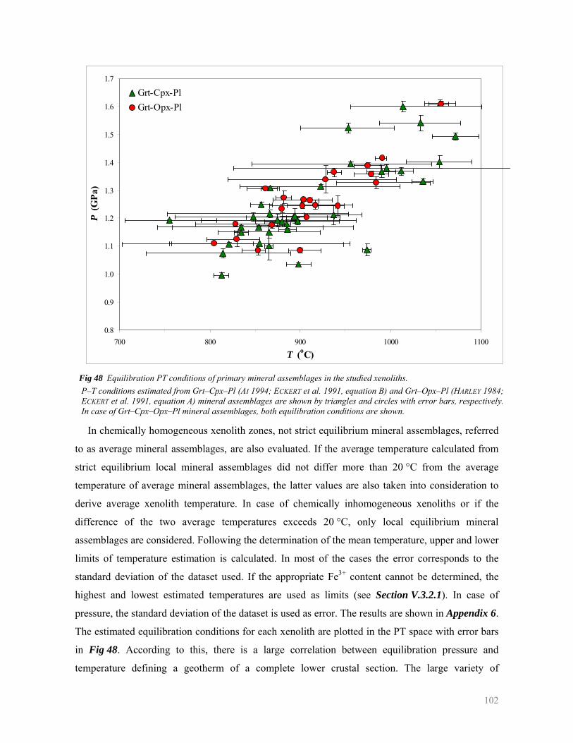
102
0.8
0.9
1.0
1.1
1.2
1.3
1.4
1.5
1.6
1.7
700 800 900 1000 1100
T (oC)
P (G
Pa)
Grt-Cpx-PlGrt-Opx-Pl
Fig 48 Equilibration PT conditions of primary mineral assemblages in the studied xenoliths. P–T conditions estimated from Grt–Cpx–Pl (AI 1994; ECKERT et al. 1991, equation B) and Grt–Opx–Pl (HARLEY 1984; ECKERT et al. 1991, equation A) mineral assemblages are shown by triangles and circles with error bars, respectively. In case of Grt–Cpx–Opx–Pl mineral assemblages, both equilibration conditions are shown.
In chemically homogeneous xenolith zones, not strict equilibrium mineral assemblages, referred
to as average mineral assemblages, are also evaluated. If the average temperature calculated from
strict equilibrium local mineral assemblages did not differ more than 20 °C from the average
temperature of average mineral assemblages, the latter values are also taken into consideration to
derive average xenolith temperature. In case of chemically inhomogeneous xenoliths or if the
difference of the two average temperatures exceeds 20 °C, only local equilibrium mineral
assemblages are considered. Following the determination of the mean temperature, upper and lower
limits of temperature estimation is calculated. In most of the cases the error corresponds to the
standard deviation of the dataset used. If the appropriate Fe3+ content cannot be determined, the
highest and lowest estimated temperatures are used as limits (see Section V.3.2.1). In case of
pressure, the standard deviation of the dataset is used as error. The results are shown in Appendix 6.
The estimated equilibration conditions for each xenolith are plotted in the PT space with error bars
in Fig 48. According to this, there is a large correlation between equilibration pressure and
temperature defining a geotherm of a complete lower crustal section. The large variety of

103
equilibrium PT conditions is observed because different xenoliths sample different crustal depths.
Since the lowest recorded pressure (i.e. the shallowest depth) well exceeds the highest crustal
pressures in the present day lower crust (approximately 0.8 GPa from the depth of the crust mantle
boundary beneath the area; POSGAY et al. 1991). The geotherm preserved by the primary mineral
assemblages corresponds to a paleogeotherm of the Alpine orogeny.
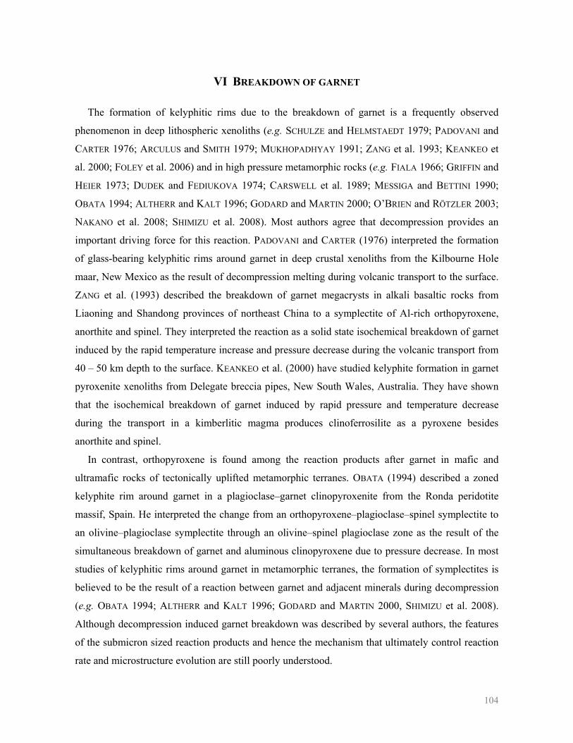
104
VI BREAKDOWN OF GARNET
The formation of kelyphitic rims due to the breakdown of garnet is a frequently observed
phenomenon in deep lithospheric xenoliths (e.g. SCHULZE and HELMSTAEDT 1979; PADOVANI and
CARTER 1976; ARCULUS and SMITH 1979; MUKHOPADHYAY 1991; ZANG et al. 1993; KEANKEO et
al. 2000; FOLEY et al. 2006) and in high pressure metamorphic rocks (e.g. FIALA 1966; GRIFFIN and
HEIER 1973; DUDEK and FEDIUKOVA 1974; CARSWELL et al. 1989; MESSIGA and BETTINI 1990;
OBATA 1994; ALTHERR and KALT 1996; GODARD and MARTIN 2000; O’BRIEN and RÖTZLER 2003;
NAKANO et al. 2008; SHIMIZU et al. 2008). Most authors agree that decompression provides an
important driving force for this reaction. PADOVANI and CARTER (1976) interpreted the formation
of glass-bearing kelyphitic rims around garnet in deep crustal xenoliths from the Kilbourne Hole
maar, New Mexico as the result of decompression melting during volcanic transport to the surface.
ZANG et al. (1993) described the breakdown of garnet megacrysts in alkali basaltic rocks from
Liaoning and Shandong provinces of northeast China to a symplectite of Al-rich orthopyroxene,
anorthite and spinel. They interpreted the reaction as a solid state isochemical breakdown of garnet
induced by the rapid temperature increase and pressure decrease during the volcanic transport from
40 – 50 km depth to the surface. KEANKEO et al. (2000) have studied kelyphite formation in garnet
pyroxenite xenoliths from Delegate breccia pipes, New South Wales, Australia. They have shown
that the isochemical breakdown of garnet induced by rapid pressure and temperature decrease
during the transport in a kimberlitic magma produces clinoferrosilite as a pyroxene besides
anorthite and spinel.
In contrast, orthopyroxene is found among the reaction products after garnet in mafic and
ultramafic rocks of tectonically uplifted metamorphic terranes. OBATA (1994) described a zoned
kelyphite rim around garnet in a plagioclase–garnet clinopyroxenite from the Ronda peridotite
massif, Spain. He interpreted the change from an orthopyroxene–plagioclase–spinel symplectite to
an olivine–plagioclase symplectite through an olivine–spinel plagioclase zone as the result of the
simultaneous breakdown of garnet and aluminous clinopyroxene due to pressure decrease. In most
studies of kelyphitic rims around garnet in metamorphic terranes, the formation of symplectites is
believed to be the result of a reaction between garnet and adjacent minerals during decompression
(e.g. OBATA 1994; ALTHERR and KALT 1996; GODARD and MARTIN 2000, SHIMIZU et al. 2008).
Although decompression induced garnet breakdown was described by several authors, the features
of the submicron sized reaction products and hence the mechanism that ultimately control reaction
rate and microstructure evolution are still poorly understood.
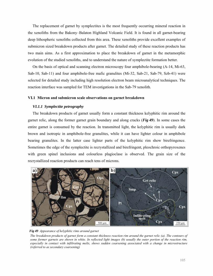
105
The replacement of garnet by symplectites is the most frequently occurring mineral reaction in
the xenoliths from the Bakony–Balaton Highland Volcanic Field. It is found in all garnet-bearing
deep lithospheric xenoliths collected from this area. These xenoliths provide excellent examples of
submicron sized breakdown products after garnet. The detailed study of these reaction products has
two main aims. As a first approximation to place the breakdown of garnet in the metamorphic
evolution of the studied xenoliths, and to understand the nature of symplectite formation better.
On the basis of optical and scanning electron microscopy four amphibole-bearing (A-14, Mi-63,
Sab-10, Sab-11) and four amphibole-free mafic granulites (Mi-32, Sab-21, Sab-79, Szb-41) were
selected for detailed study including high resolution electron beam microanalytical techniques. The
reaction interface was sampled for TEM investigations in the Sab-79 xenolith.
VI.1 Micron and submicron scale observations on garnet breakdown
VI.1.1 Symplectite petrography
The breakdown products of garnet usually form a constant thickness kelyphitic rim around the
garnet relic, along the former garnet grain boundary and along cracks (Fig 49). In some cases the
entire garnet is consumed by the reaction. In transmitted light, the kelyphitic rim is usually dark
brown and isotropic in amphibole-free granulites, while it can have lighter colour in amphibole
bearing granulites. In the latter case lighter parts of the kelyphitic rim show birefringence.
Sometimes the edge of the symplectite is recrystallized and birefringent, pleochroic orthopyroxenes
with green spinel inclusions and colourless plagioclase is observed. The grain size of the
recrystallized reaction products can reach tens of microns.
Fig 49 Appearance of kelyphitic rims around garnet The breakdown products of garnet form a constant thickness reaction rim around the garnet relic (a). The contours of some former garnets are shown in white. In reflected light images (b) usually the outer portion of the reaction rim, especially in contact with infiltrating melts, shows sudden coarsening associated with a change in microstructure (referred to as secondary coarsening)
106
Backscattered electron images (Fig 50) show that in all mafic granulite xenoliths the kelyphitic
rim consists of an orthopyroxene–plagioclase–spinel mineral assemblage referred to as type 1
symplectite. The interface between the precursor garnet and the aggregate of the symplectite phases
is extremely sharp. The width of the reaction rim is independent of the nature of the adjacent
phases. The inner part of the reaction rim is comprised of submicron sized reaction products
forming vermicular intergrowths. I refer to this microstructure as fine-grained symplectite. The
grain size of the fine-grained symplectites continuously increases from the reaction front towards
the former garnet boundary (Fig 50ab), whereas the microstructure is consistent. This phenomenon
is referred as primary coarsening.
In most of the cases, a sudden change in grain size and microstructure within the type 1
symplectite is observed at the former garnet grain boundary or along cracks (Fig 50c). Although
the mineralogy of the reaction product remains constant, the grain size may suddenly increase from
the submicron scale to tens of microns. At the same time, the vermicular microstructure is
transferred into an intergrowth of subhedral or euhedral orthopyroxene, plagioclase and spinel. This
phenomenon is particularly pronounced, when a hydroxyl bearing mineral showing signs of melting
or infiltrating host basalt is present close to the garnet (Fig 49b). This type of coarsening associated
with microstructural variations is referred to as secondary coarsening.
In some amphibole-bearing granulites, the original microstructure of the fine-grained
symplectite is partly or completely obliterated by radial channels, which widen from the garnet–
symplectite interface towards the former grain boundary (Fig 50d), which they usually do not
reach. Alternating dark and light grey channels are observed on the BSE image, which reflects
different composition. Crystalline phases are not involved in this microstructure.
Type 1 symplectite in some cases reacts with melts to form a second generation of symplectite,
referred to as type 2 symplectite, which consists of an olivine–plagioclase–spinel ± orthopyroxene
± melt mineral assemblage. This mineral assemblage and its relations to infiltrating melts has been
described in Section IV.1.2.1.
VI.1.2 Symplectite chemistry
Two types of electron microprobe analyses were performed in type 1 symplectite. The average
composition of the fine-grained symplectite was determined with defocused electron beam, while
point analyses were done on individual phases in the recrystallized parts. The results are shown in
Table 8.
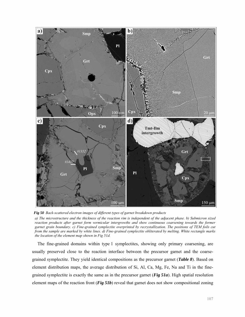
107
Fig 50 Back-scattered electron images of different types of garnet breakdown products a) The microstructure and the thickness of the reaction rim is independent of the adjacent phase. b) Submicron sized reaction products after garnet form vermicular intergrowths and show continuous coarsening towards the former garnet grain boundary. c) Fine-grained symplectite overprinted by recrystallization. The positions of TEM foils cut from the sample are marked by white lines. d) Fine-grained symplectite obliterated by melting. White rectangle marks the location of the element map shown in Fig 51d.
The fine-grained domains within type 1 symplectites, showing only primary coarsening, are
usually preserved close to the reaction interface between the precursor garnet and the coarse-
grained symplectite. They yield identical compositions as the precursor garnet (Table 8). Based on
element distribution maps, the average distribution of Si, Al, Ca, Mg, Fe, Na and Ti in the fine-
grained symplectite is exactly the same as in the precursor garnet (Fig 51a). High spatial resolution
element maps of the reaction front (Fig 51b) reveal that garnet does not show compositional zoning
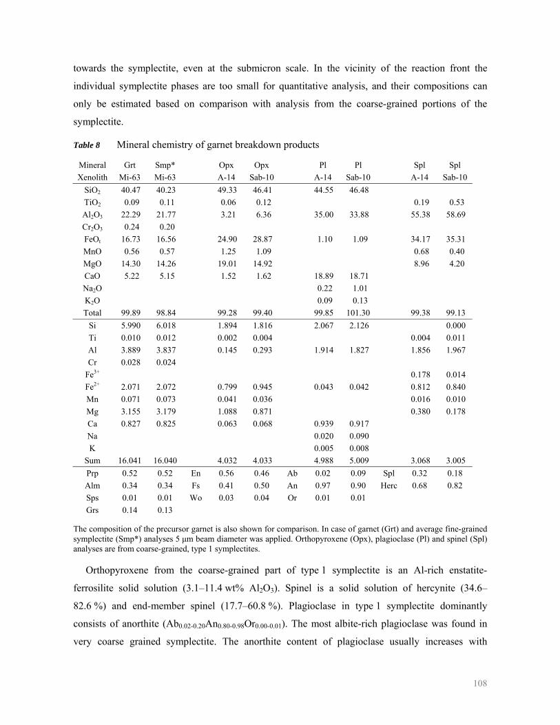
108
towards the symplectite, even at the submicron scale. In the vicinity of the reaction front the
individual symplectite phases are too small for quantitative analysis, and their compositions can
only be estimated based on comparison with analysis from the coarse-grained portions of the
symplectite.
Table 8 Mineral chemistry of garnet breakdown products
Mineral Grt Smp* Opx Opx Pl Pl Spl Spl Xenolith Mi-63 Mi-63 A-14 Sab-10 A-14 Sab-10 A-14 Sab-10
SiO2 40.47 40.23 49.33 46.41 44.55 46.48 TiO2 0.09 0.11 0.06 0.12 0.19 0.53 Al2O3 22.29 21.77 3.21 6.36 35.00 33.88 55.38 58.69 Cr2O3 0.24 0.20 FeOt 16.73 16.56 24.90 28.87 1.10 1.09 34.17 35.31 MnO 0.56 0.57 1.25 1.09 0.68 0.40 MgO 14.30 14.26 19.01 14.92 8.96 4.20 CaO 5.22 5.15 1.52 1.62 18.89 18.71 Na2O 0.22 1.01 K2O 0.09 0.13 Total 99.89 98.84 99.28 99.40 99.85 101.30 99.38 99.13
Si 5.990 6.018 1.894 1.816 2.067 2.126 0.000 Ti 0.010 0.012 0.002 0.004 0.004 0.011 Al 3.889 3.837 0.145 0.293 1.914 1.827 1.856 1.967 Cr 0.028 0.024
Fe3+ 0.178 0.014 Fe2+ 2.071 2.072 0.799 0.945 0.043 0.042 0.812 0.840 Mn 0.071 0.073 0.041 0.036 0.016 0.010 Mg 3.155 3.179 1.088 0.871 0.380 0.178 Ca 0.827 0.825 0.063 0.068 0.939 0.917 Na 0.020 0.090 K 0.005 0.008
Sum 16.041 16.040 4.032 4.033 4.988 5.009 3.068 3.005 Prp 0.52 0.52 En 0.56 0.46 Ab 0.02 0.09 Spl 0.32 0.18 Alm 0.34 0.34 Fs 0.41 0.50 An 0.97 0.90 Herc 0.68 0.82 Sps 0.01 0.01 Wo 0.03 0.04 Or 0.01 0.01 Grs 0.14 0.13
The composition of the precursor garnet is also shown for comparison. In case of garnet (Grt) and average fine-grained symplectite (Smp*) analyses 5 μm beam diameter was applied. Orthopyroxene (Opx), plagioclase (Pl) and spinel (Spl) analyses are from coarse-grained, type 1 symplectites.
Orthopyroxene from the coarse-grained part of type 1 symplectite is an Al-rich enstatite-
ferrosilite solid solution (3.1–11.4 wt% Al2O3). Spinel is a solid solution of hercynite (34.6–
82.6 %) and end-member spinel (17.7–60.8 %). Plagioclase in type 1 symplectite dominantly
consists of anorthite (Ab0.02-0.20An0.80-0.98Or0.00-0.01). The most albite-rich plagioclase was found in
very coarse grained symplectite. The anorthite content of plagioclase usually increases with
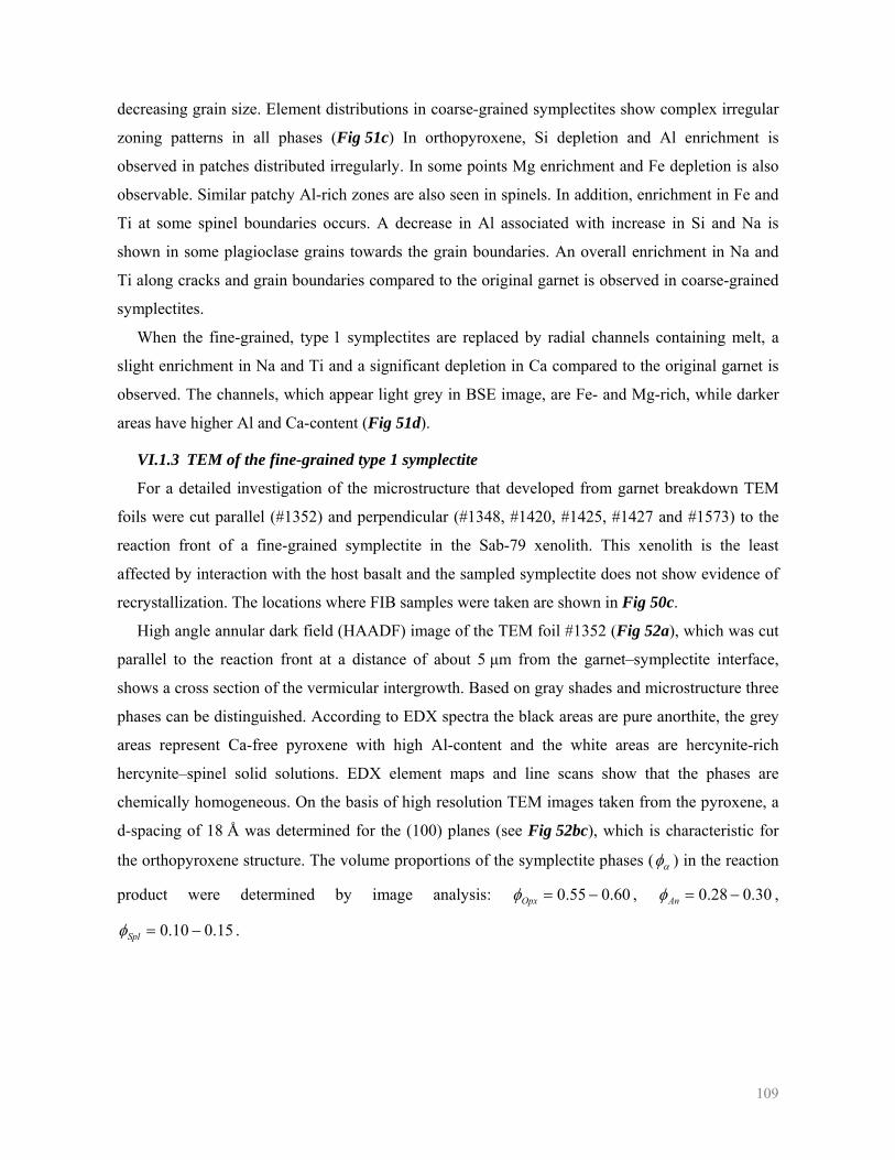
109
decreasing grain size. Element distributions in coarse-grained symplectites show complex irregular
zoning patterns in all phases (Fig 51c) In orthopyroxene, Si depletion and Al enrichment is
observed in patches distributed irregularly. In some points Mg enrichment and Fe depletion is also
observable. Similar patchy Al-rich zones are also seen in spinels. In addition, enrichment in Fe and
Ti at some spinel boundaries occurs. A decrease in Al associated with increase in Si and Na is
shown in some plagioclase grains towards the grain boundaries. An overall enrichment in Na and
Ti along cracks and grain boundaries compared to the original garnet is observed in coarse-grained
symplectites.
When the fine-grained, type 1 symplectites are replaced by radial channels containing melt, a
slight enrichment in Na and Ti and a significant depletion in Ca compared to the original garnet is
observed. The channels, which appear light grey in BSE image, are Fe- and Mg-rich, while darker
areas have higher Al and Ca-content (Fig 51d).
VI.1.3 TEM of the fine-grained type 1 symplectite
For a detailed investigation of the microstructure that developed from garnet breakdown TEM
foils were cut parallel (#1352) and perpendicular (#1348, #1420, #1425, #1427 and #1573) to the
reaction front of a fine-grained symplectite in the Sab-79 xenolith. This xenolith is the least
affected by interaction with the host basalt and the sampled symplectite does not show evidence of
recrystallization. The locations where FIB samples were taken are shown in Fig 50c.
High angle annular dark field (HAADF) image of the TEM foil #1352 (Fig 52a), which was cut
parallel to the reaction front at a distance of about 5 μm from the garnet–symplectite interface,
shows a cross section of the vermicular intergrowth. Based on gray shades and microstructure three
phases can be distinguished. According to EDX spectra the black areas are pure anorthite, the grey
areas represent Ca-free pyroxene with high Al-content and the white areas are hercynite-rich
hercynite–spinel solid solutions. EDX element maps and line scans show that the phases are
chemically homogeneous. On the basis of high resolution TEM images taken from the pyroxene, a
d-spacing of 18 Å was determined for the (100) planes (see Fig 52bc), which is characteristic for
the orthopyroxene structure. The volume proportions of the symplectite phases ( αφ ) in the reaction
product were determined by image analysis: 60.055.0 −=Opxφ , 30.028.0 −=Anφ ,
15.010.0 −=Splφ .
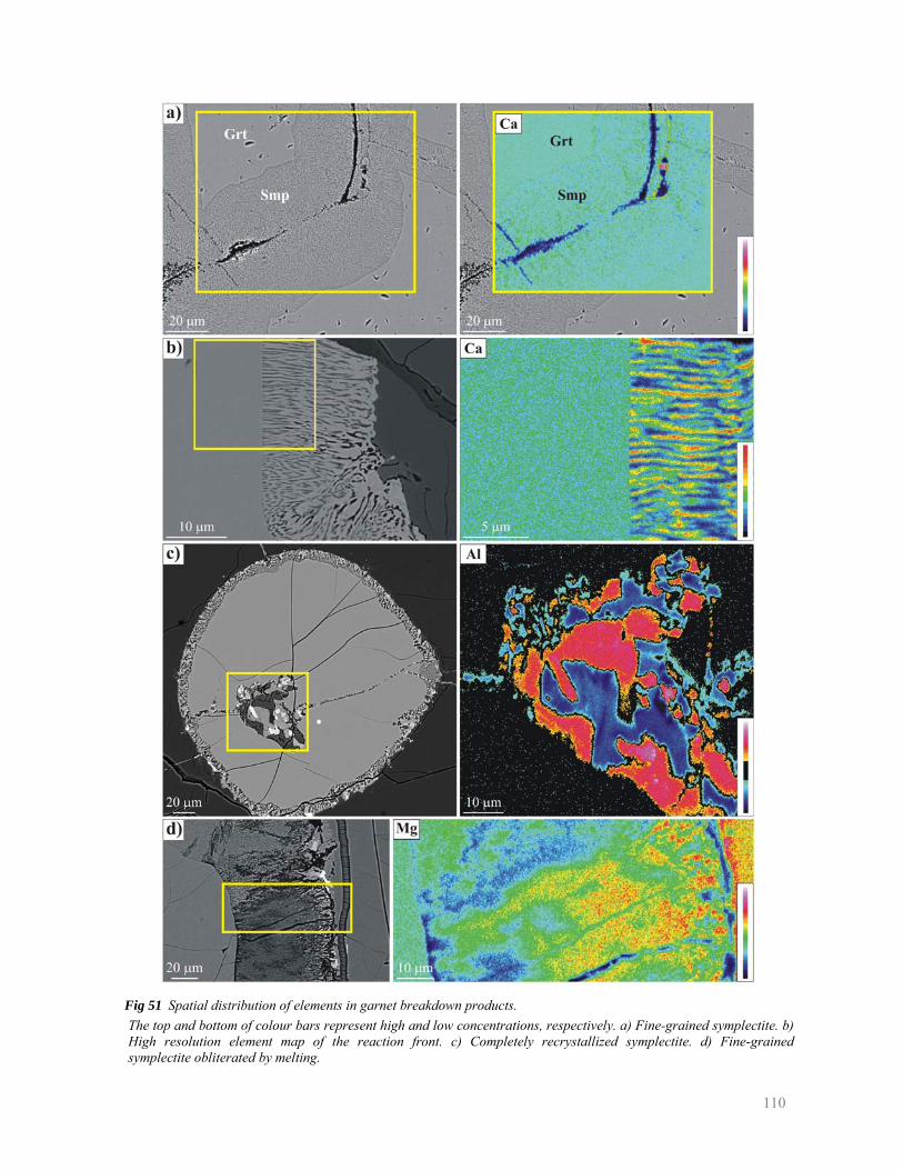
110
Fig 51 Spatial distribution of elements in garnet breakdown products. The top and bottom of colour bars represent high and low concentrations, respectively. a) Fine-grained symplectite. b) High resolution element map of the reaction front. c) Completely recrystallized symplectite. d) Fine-grained symplectite obliterated by melting.
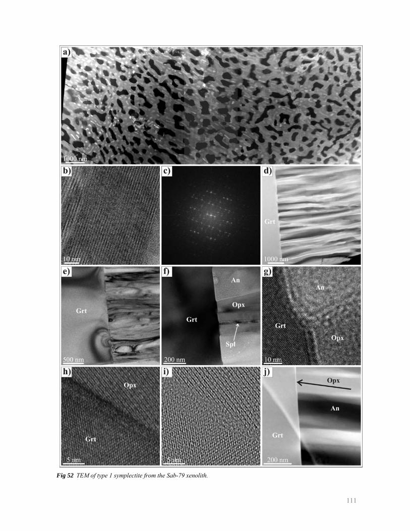
111
Fig 52 TEM of type 1 symplectite from the Sab-79 xenolith.
112
Caption of Fig 52 above: a) HAADF image of the TEM foil #1352 cut parallel to the reaction front at a distance of 5 μm from the front. Pure anorthite, Al-rich orthopyroxene and hercynitic spinel appear as black, grey and white phases, respectively. b) Energy filtered high resolution image of an orthopyroxene from the fine-grained symplectite showing 18 Å lattice spacing of the (100) planes. c) Diffraction pattern of orthopyroxene from the fine-grained symplectite. Fast Fourier Transform (FFT) of Fig 52b. d) HAADF overview of the TEM foil #1420 cut perpendicular to the reaction front. e) Bright field image of the reaction front. Strain contrast centers are visible at the garnet–symplectite interface. f) Bright field image showing the nanoscale topography of the reaction front. Anorthite protrudes deeper into the garnet than orthopyroxene and spinel. g) High resolution image of an anorthite–orthopyroxene–garnet ‘triple junction’ at the reaction front. A 5 nm step is observable within the reaction front. h) High resolution image of the reaction front between garnet and orthopyroxene. A 2 – 5 nm wide disordered zone is observed within the garnet right at the reaction front. i) Filtered high resolution image of the reaction front (Fig 52h) applying a bandpass mask to the diffraction pattern (fast Fourier Transform FFT) and calculating the inverse FFT. This technique excludes the primary beam from the image calculation and some noise intensity around the primary beam in the diffraction pattern (c.f. DE JONG et al. 1989). j) HAADF image of the reaction front. A narrow, bright zone associated with slight Fe-enrichment, marked by an arrow, is observed. The curved bright band across the image is an artefact due to the underlying perforated carbon film on which part of the foil rests.
The internal microstructure of the symplectite is consistent within the foil. Anorthite forms
about 200 nm thick rods oriented sub-perpendicular to the reaction front. These rods are surrounded
by orthopyroxene, which forms the matrix of the symplectite. Spinel is only found within the
orthopyroxene, where it forms discontinuous rods of about 20 nm width, which are also oriented
sub-perpendicular to the reaction front. No coherent interphase boundaries were detected in high
resolution images. Triple junctions were frequently observed.
In TEM foils cut perpendicular to the reaction front the reaction products seem to have lamellar
structure sub-perpendicular to the garnet–symplectite interphase boundary (Fig 52d–g). Bright field
images reveal strain contrast centers in the garnet close to the reaction front and also in the
symplectite phases (Fig 52e). All three symplectite phases seem to nucleate on the reaction front,
but anorthite systematically propagates deeper into the garnet than orthopyroxene and spinel
(Fig 52f). This gives a subtle topography to the reaction front with 5 nm steps at the triple junctions
between two symplectite phases and the precursor garnet (Fig 52g).
High resolution TEM images of the reaction front show that the atomic structure of the reactant
garnet is partially disturbed within a 2–5 nm wide zone right at the interface to the symplectite
(Fig 52hi). No amorphous material or indication for a fluid phase is found along the reaction front.
On the other hand, a few nanometer wide very consistent zone along the garnet–symplectite
interface was detected, which appears to be brighter in the HAADF images (Fig 52j) than the
surrounding phases and which coincides with the partially disordered zone of the garnet. According
to the results of EDX line analyses perpendicular to the reaction front and area EDX measurements
within the garnet and at the interface, the zone of disordered garnet is slightly enriched in Fe
relative to its surroundings.
113
VI.2 Processes involved in symplectite formation
The formation of kelyphitic rims around garnet is the result of complex processes during the
metamorphic evolution of the lower crust. The constant thickness of these reaction rims around
garnet with a microstructure independent of the adjacent phase suggests that garnet was the only
solid reactant involved in kelyphite formation. According to detailed microstructural observations,
all garnet grains react to form a symplectite of Al-rich orthopyroxene, pure anorthite and hercynitic
spinel (type 1 symplectite) along a sharp reaction front. In some samples, an olivine, plagioclase,
spinel ± orthopyroxene ± melt mineral assemblage (type 2 symplectite) is also observed within the
kelyphitic rim. Type 2 symplectites always grow on the expense of type 1 symplectites and they
never have a common interface with the garnet relic. This clearly demonstrates that garnet
breakdown to form type 1 symplectites anticipates the formation of type 2 symplectites.
According to element distributions and microprobe analyses with a defocussed electron beam on
the fine-grained symplectite, the breakdown of garnet to a vermicular intergrowth of submicron
sized Al-rich orthopyroxene, pure anorthite and hercynitic spinel close to the reaction front is
isochemical. The only late alteration observed within these reaction products preserving garnet
composition is primary coarsening, which affects only grain size and does not cause changes in the
microstructure. No indication was found for the presence of a free fluid during this process.
However, further alterations, such as secondary coarsening, the reaction to form type 2 symplectite
and the formation of radial channels within the fine-grained symplectites all seem to be
metasomatic in nature.
Secondary coarsening involves sudden change of the grain size as well as of the microstructure
together with the addition of Na, K and Ti to the system. Theoretically, the increase of Na content
can be the result of a reaction with the surrounding clinopyroxene, as these contain up to 1.5 wt%
Na2O. This reaction does, however, not explain the increase of K and Ti towards grain boundaries
and cracks. The enrichment of these elements is restricted to areas close to cracks and grain
boundaries, which suggests the presence of a fluid or melt phase during recrystallization. The host
alkali basalt provides the most probable external source for these elements. This view is also
corroborated by the fact that secondary coarsening is more pronounced close to partially molten
amphiboles and melt pockets or films of infiltrating host basalt (Fig 49b).
Type 2 symplectites always occur in kelyphitic rims which are in connection with infiltrating
host basalt. In addition, the composition of the minerals in this assemblage much more resemble to
the same phases crystallized from the basalt than to phases of type 1 symplectite (see
Section IV.2.2). On this basis, the formation of type 2 (olivine–plagioclase–
114
spinel±orthopyroxene±melt) symplectite can also be interpreted as the result of a reaction between
the fine-grained type 1 symplectite and the host melt.
The formation of radial channels in the garnet breakdown products may be the result of melting
at the reaction front, where the interfacial energy is high due to the small grain size. This process is
observed only in amphibole-bearing samples, which suggests that the thermal interaction between
the host basalt and the xenolith together with the relatively high water activity of the generated and
infiltrated melts induced melting of the fine-grained symplectite.
VI.3 Thermodynamic analysis of isochemical garnet breakdown
VI.3.1 Mass balance considerations
Reaction stoichiometry of the isochemical breakdown of garnet to form type 1 symplectite in the
Sab-79 xenolith has been determined on the basis of mass balance considerations. A list of
frequently used symbols is found in Appendix 10.
According to TEM observations, the plagioclase in the isochemical type 1 symplectite occurs as
pure anorthite, while the spinel is very hercynite-rich. By using the assumption that the spinel is
pure hercynite, the following chemical reaction can be derived:
(Fe,Mg,Ca)3Al2Si3O12 = Anν CaAl2Si2O8 + Opxν (Fe,Mg,Ca,Al)2(Al,Si)2O6 + Splν FeAl2O4
Grt An Opx Hc
where αν refers to the molar proportion of phase α in the reaction product. This equation contains
8 unknowns, the Si-, Al-, Fe-, Mg- and Ca-content of orthopyroxene and the molar proportions of
the symplectite phases. The molar proportions of the symplectite phases ( αν ) are directly related to
their volume proportions in the symplectite (Smp
a VVαφ = ) through the following equations where αV
and αV refer to the volume and the molar volume of phase α , respectively:
ααα ν VV ⋅= and β
β
β
α
β
α
φφ
νν
VV
⋅= .
If we assume that the orthopyroxene has stoichiometric composition, a linear relationship exists
among the numbers of atoms per formula unit of the components (i) in orthopyroxene ( Opxin ):
4=++++ OpxCa
OpxMg
OpxFe
OpxAl
OpxSi nnnnn .
Eq 19 The mass balance of the chemical components in the garnet breakdown reaction may be
expressed by the following equations:
115
OpxCaOpx
AnCaAn
GrtCa nnn ⋅+⋅= νν
Eq 20 OpxSiOpx
AnSiAn
GrtSi nnn ⋅+⋅= νν
Eq 21 SplAlSpl
OpxAlOpx
AnAlAn
GrtAl nnnn ⋅+⋅+⋅= ννν
Eq 22 SplFeSpl
OpxFeOpx
GrtFe nnn ⋅+⋅= νν
Eq 23 OpxMgOpx
GrtMg nn ⋅=ν
Eq 24 If we express all unknowns as a function of the Ca-content in orthopyroxene, we can change this
value as a parameter until Eq 19 is satisfied. The resulting reaction stoichiometry for the studied
garnet grain reads:
Fe1.44Mg1.02Ca0.48Al2Si3O12 = 0.40 CaAl2Si2O8 + 1.24 Fe0.89Mg0.82Ca0.07Al0.44Si1.77O6+ 0.33 FeAl2O4
Grt An Opx Hc
The uncertainties in the estimation of the volume fraction of the symplectite phases can cause
some variations in the calculated stoichiometry. They primarily affect the Al-content of the
orthopyroxene, which may vary between 0.27 and 0.44 atoms per formula unit if ±5 % uncertainty
is assumed in the determination of mineral modes in the symplectite.
VI.3.2 Equilibrium phase relations
The phase relations of isochemical garnet breakdown were investigated by constructing
pseudosections for the composition of the precursor garnet in the CaO–FeO–MgO–Al2O3–SiO2
(CFMAS) system. The calculations were done using the PERPLEX software (CONNOLLY 1990)
and the database and solution models of HOLLAND and POWELL (1998). According to the
pseudosection, garnet is stable at high pressures and it reacts to form an orthopyroxene–anorthite–
spinel mineral assemblage towards lower pressures. The four phase assemblage
Grt + An + Opx + Spl defines a narrow field with a shallow overall positive slope on the P–T
diagram (Fig 53). Garnet starts to react out at the upper stability limit of this field, and its modal
proportion continuously decreases towards the lower stability limit, where it goes to zero. The
position of this four phase field is sensitive to the composition of the precursor garnet. During
decompression at 1000 °C the most Mg-rich garnet from mafic granulites (Prp: 52%) is predicted to
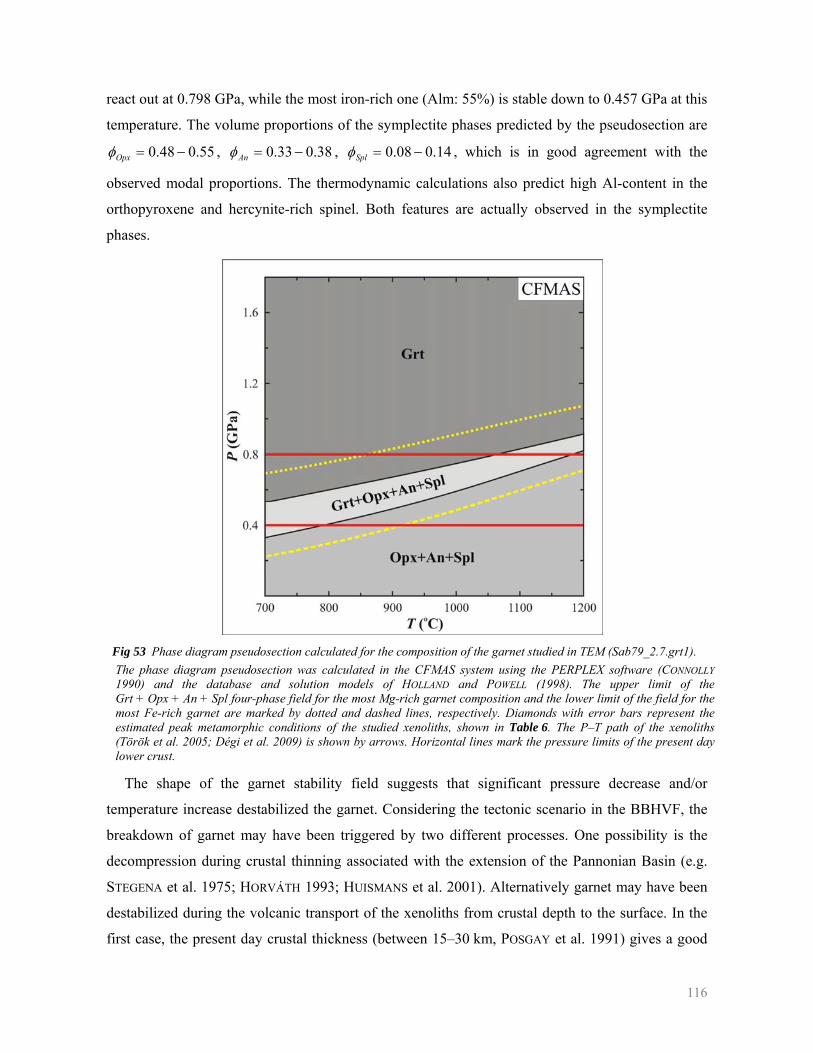
116
react out at 0.798 GPa, while the most iron-rich one (Alm: 55%) is stable down to 0.457 GPa at this
temperature. The volume proportions of the symplectite phases predicted by the pseudosection are
55.048.0 −=Opxφ , 38.033.0 −=Anφ , 14.008.0 −=Splφ , which is in good agreement with the
observed modal proportions. The thermodynamic calculations also predict high Al-content in the
orthopyroxene and hercynite-rich spinel. Both features are actually observed in the symplectite
phases.
Fig 53 Phase diagram pseudosection calculated for the composition of the garnet studied in TEM (Sab79_2.7.grt1). The phase diagram pseudosection was calculated in the CFMAS system using the PERPLEX software (CONNOLLY 1990) and the database and solution models of HOLLAND and POWELL (1998). The upper limit of the Grt + Opx + An + Spl four-phase field for the most Mg-rich garnet composition and the lower limit of the field for the most Fe-rich garnet are marked by dotted and dashed lines, respectively. Diamonds with error bars represent the estimated peak metamorphic conditions of the studied xenoliths, shown in Table 6. The P–T path of the xenoliths (Török et al. 2005; Dégi et al. 2009) is shown by arrows. Horizontal lines mark the pressure limits of the present day lower crust.
The shape of the garnet stability field suggests that significant pressure decrease and/or
temperature increase destabilized the garnet. Considering the tectonic scenario in the BBHVF, the
breakdown of garnet may have been triggered by two different processes. One possibility is the
decompression during crustal thinning associated with the extension of the Pannonian Basin (e.g.
STEGENA et al. 1975; HORVÁTH 1993; HUISMANS et al. 2001). Alternatively garnet may have been
destabilized during the volcanic transport of the xenoliths from crustal depth to the surface. In the
first case, the present day crustal thickness (between 15–30 km, POSGAY et al. 1991) gives a good
117
constraint on the pressure conditions (0.4–0.8 GPa) of the lower crust after the extension of the
Pannonian Basin. According to the results of thermobarometry, only a slight increase in
temperature to a maximum of 1000–1100 °C could take place in the lower crust during lithosphere
thinning. At these temperatures, the Grt–An–Opx–Spl four-phase field on the pseudosection plots
in the depth range of the present day lower crust (Fig 53). This means that the pressure
overstepping of the garnet stability field was very small, most probably less than 0.1 GPa. If garnet
breakdown had indeed occurred during decompression associated with crustal thinning in the lower
crust, the reaction may have taken place very close to equilibrium conditions, where GrΔ → 0. If,
in the alternative scenario, the reaction was induced by decompression during the volcanic transport
of the xenoliths to the surface, the pressure overstepping could amount to 0.8 GPa. The temperature
of the xenoliths during their interaction with the host basalt could get close to the temperature of the
basalt (1220–1270 °C, KÓTHAY et al. 2005). This results in extremely large reaction affinity, where
GrΔ is in the range of kilojoules per mole of reactant garnet.
VI.3.3 Controls on symplectite formation
The nanoscale features of the garnet – symplectite interphase boundary give some initiation of
the processes that controlled symplectite formation. In all TEM foils cut perpendicular to the
reaction front, all three phases of the symplectite have common boundaries with garnet. This
suggests that all symplectite phases nucleated at the reaction front.
The presence of strain contrast centres along the garnet – symplectite interphase boundary are
probably related to volume change during symplectite formation. According to the phase diagram
pseudosection, the reaction results in nearly 15 % volume increase, which can lead to the distortion
of the crystal lattices. The presence of the 2 – 5 nm wide disordered zone along the garnet –
symplectite interphase boundary supports this argument. Since no indication for the presence of a
fluid phase along the interphase boundary was found, most likely the disordered zone served as a
fast diffusion pathway where the chemical separation that is necessary during replacement of the
garnet by the symplectite assemblage took place. The regular spacing of the symplectite phases
along the reaction front suggests that their nucleation and growth is indeed diffusion controlled.
VI.3.4 Thermodynamic model for symplectite formation
Based on the observations on natural symplectites after garnet in lower crustal mafic xenoliths
of the BBHVF a thermodynamic model was developed to analyse the kinetics of symplectite
formation using the principles of irreversible thermodynamics. The model was formulated by Prof.
Rainer Abart, I took part in the testing and programming part of the work.
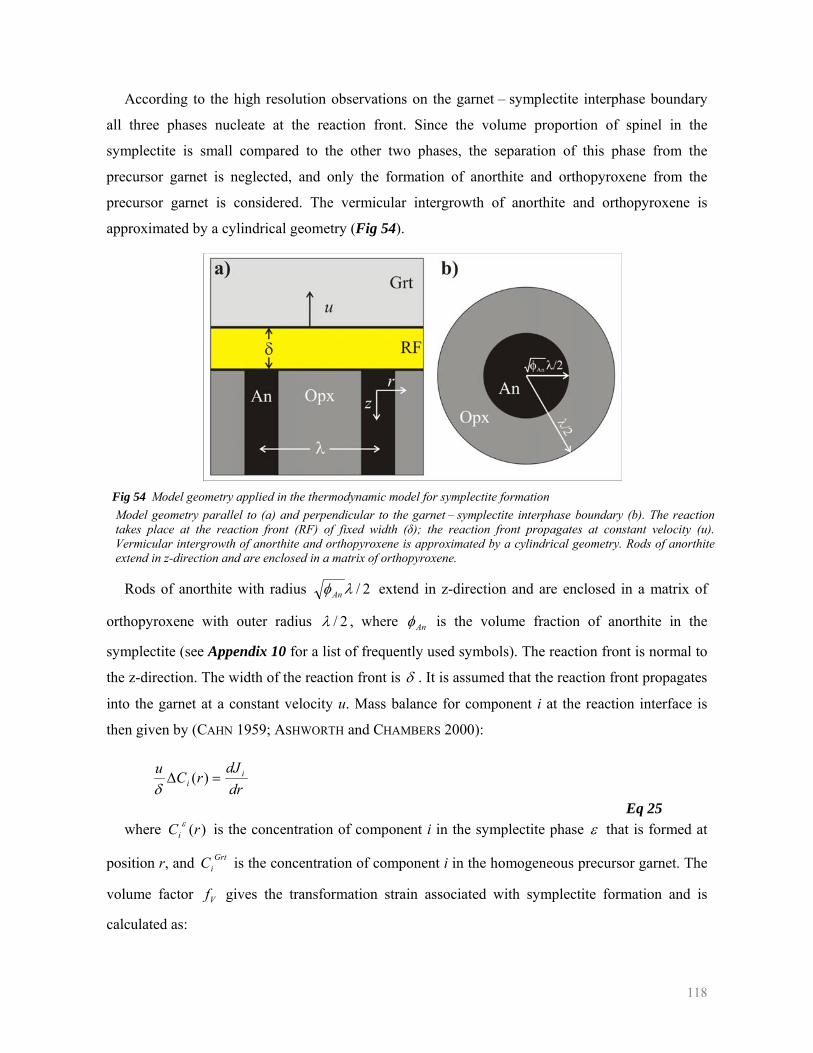
118
According to the high resolution observations on the garnet – symplectite interphase boundary
all three phases nucleate at the reaction front. Since the volume proportion of spinel in the
symplectite is small compared to the other two phases, the separation of this phase from the
precursor garnet is neglected, and only the formation of anorthite and orthopyroxene from the
precursor garnet is considered. The vermicular intergrowth of anorthite and orthopyroxene is
approximated by a cylindrical geometry (Fig 54).
Fig 54 Model geometry applied in the thermodynamic model for symplectite formation Model geometry parallel to (a) and perpendicular to the garnet – symplectite interphase boundary (b). The reaction takes place at the reaction front (RF) of fixed width (δ); the reaction front propagates at constant velocity (u). Vermicular intergrowth of anorthite and orthopyroxene is approximated by a cylindrical geometry. Rods of anorthite extend in z-direction and are enclosed in a matrix of orthopyroxene.
Rods of anorthite with radius 2/λφAn extend in z-direction and are enclosed in a matrix of
orthopyroxene with outer radius 2/λ , where Anφ is the volume fraction of anorthite in the
symplectite (see Appendix 10 for a list of frequently used symbols). The reaction front is normal to
the z-direction. The width of the reaction front is δ . It is assumed that the reaction front propagates
into the garnet at a constant velocity u. Mass balance for component i at the reaction interface is
then given by (CAHN 1959; ASHWORTH and CHAMBERS 2000):
drdJ
rCu ii =Δ )(
δ
Eq 25 where )(rCi
ε is the concentration of component i in the symplectite phase ε that is formed at
position r, and GrtiC is the concentration of component i in the homogeneous precursor garnet. The
volume factor Vf gives the transformation strain associated with symplectite formation and is
calculated as:
119
GrtGrt
AnAnOpxOpxV V
VVf
ννν
⋅
⋅+⋅= ,
where αV and αν are the molar volume and the stoichiometric coefficient of phase α ,
respectively.
For the case at hand both the compositions of the precursor garnet and the compositions of the
symplectite phases are constant, and integration of Eq 25 yields
Ani
Ani CurJ Δ=
δ2 for 2/0 λφAnr ≤≤ ,
⎟⎟⎠
⎞⎜⎜⎝
⎛−Δ= r
rCuJ Opx
iOpx
i 42
2λδ
for 2/2/ λλφ ≤≤ rAn .
Eq 26 If the re-distribution of chemical components by diffusion within the reaction interface is
considered as the only dissipative process during symplectite formation, the rate of energy
dissipation may be written as:
∫ ∑∫ ∑ +=2
2
22
0
2
2)(
2)(
λ
λφ
λφ
πδπδAn
An
i i
Opxi
i i
Ani drr
LJ
drrL
JQ& ,
Eq 27 where iL is the phenomenological coefficient of diffusion. Inserting from Eq 26 into Eq 27
yields:
( ) ( ) ( )⎥⎥⎦
⎤
⎢⎢⎣
⎡ Δ−+
Δ= ∑ ∑
i i i
Opxi
Ani
Ani
An LC
LCuQ
22
22
24
1128
φφδπλ& .
Eq 28 The rate of free energy change during symplectite formation is calculated as
⎟⎠⎞
⎜⎝⎛ +Δ= VAnr fgug φσλπλ 2
22& ,
Eq 29 where grΔ is the change in specific Gibbs free energy at the reaction front, which is calculated
from the change in free energy in molar units as GrtGrt
rr V
Ggν
Δ=Δ , and σ is the interfacial energy of
anorthite – orthopyroxene contacts.
In the case of only one kinetic variable, u in the case at hand, the extremal principle of
maximum dissipation (ONSAGER 1931; SVOBODA et al. 2005) reduces to the constraint
120
gQ && −= (ABART et al. 2009) from which we obtain an explicit expression for the reaction front
velocity:
( ) ( ) ( )∑ ∑ Δ−+
Δ
+Δ−=
i i i
Opxi
Ani
Ani
An
VAnr
LC
LC
fgu 2
22
23
1
2264
φφ
φσλ
λδ .
Eq 30 I If the mixing properties of the material within the reaction front are assumed to be ideal, then
the phenomenological coefficients of diffusion may be expressed as RT
CDL
RFi
RFi
i = , where RFiD is
the tracer diffusion coefficient of component i within the reaction front (RF).
From our observations we concluded that material re-distribution probably occurred within the
outermost few atomic layers of the garnet next to the reaction front. The characteristic spacing of
the studied symplectite in the given model geometry (Fig 54) is =λ 400 nm. As no systematic
variations in composition could be discerned along the reaction interface, GrtiC can be assumed to
be constant and iL is calculated using component concentrations in garnet. Eq 30 can be evaluated
for feasible interfacial energies and GrΔ values and for different diffusion coefficients (Fig 55).
The list of parameters used in the calculation is shown in Table 9.
In Fig 55 the tenth logarithm of time required to form a symplectite rim of 30 µm width is
shown for different rod spacings and for the range of feasible diffusion coefficients. Two scenarios
are shown, 0.1 GPa overstepping, i.e. symplectite formation in the deep crust and 0.5 GPa
overstepping, i.e. symplectite formation during volcanic transport to the surface. Calculations were
done for interfacial energies of 0.1 and 3 J/m2 in both cases.
The tracer diffusion coefficients for diffusion of Ca, Mg and Fe in garnet were taken from
GANGULY et al. (1998). The tracer diffusion coefficients of Al and Si were taken as two orders of
magnitude slower than DCa. To account for the fact that the outermost atomic layers of garnet, i.e.
the garnet immediately in front of the reaction front appears somewhat disordered, a range of
diffusion coefficients is considered ranging from the volume diffusion coefficients to 104 of these
values representing an upper estimate for grain boundary diffusion coefficients (KELLER et al.
2008) (Fig 55). Volume diffusion coefficients are calculated for 1000 °C from the relations given
by GANGULY et al. (1998). In case of small characteristic spacings ( <λ 100 nm), the dependence of
symplectite formation time on diffusion coefficients is weak as compared to the dependence on λ .
For larger spacings, the dependence on diffusion coefficients becomes much stronger. Note that for
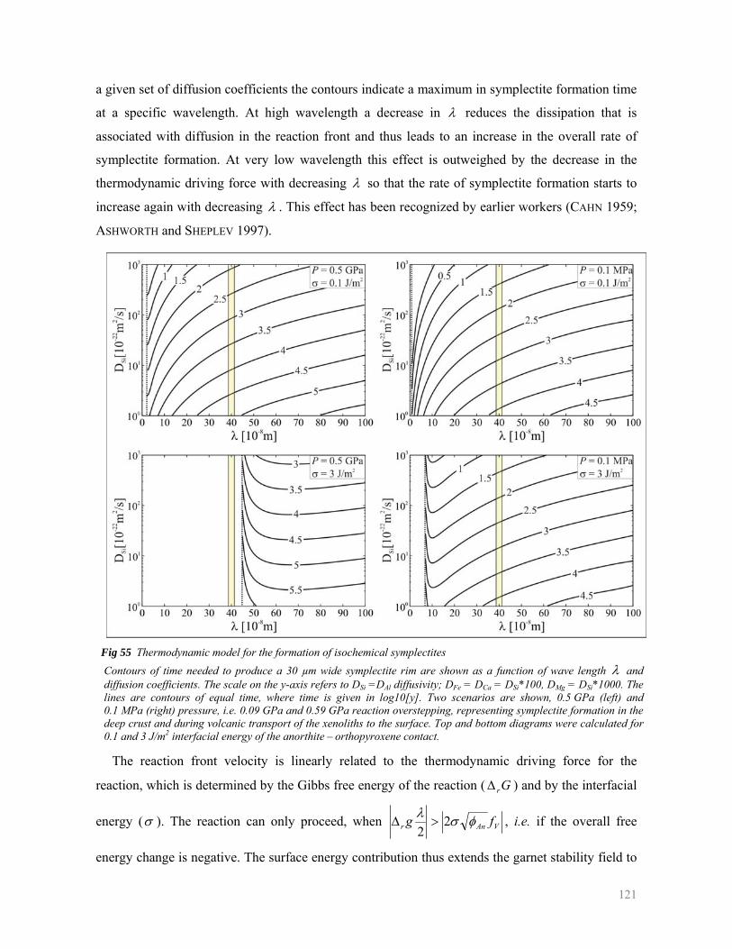
121
a given set of diffusion coefficients the contours indicate a maximum in symplectite formation time
at a specific wavelength. At high wavelength a decrease in λ reduces the dissipation that is
associated with diffusion in the reaction front and thus leads to an increase in the overall rate of
symplectite formation. At very low wavelength this effect is outweighed by the decrease in the
thermodynamic driving force with decreasing λ so that the rate of symplectite formation starts to
increase again with decreasing λ . This effect has been recognized by earlier workers (CAHN 1959;
ASHWORTH and SHEPLEV 1997).
Fig 55 Thermodynamic model for the formation of isochemical symplectites Contours of time needed to produce a 30 µm wide symplectite rim are shown as a function of wave length λ and diffusion coefficients. The scale on the y-axis refers to DSi =DAl diffusivity; DFe = DCa = DSi*100, DMg = DSi*1000. The lines are contours of equal time, where time is given in log10[y]. Two scenarios are shown, 0.5 GPa (left) and 0.1 MPa (right) pressure, i.e. 0.09 GPa and 0.59 GPa reaction overstepping, representing symplectite formation in the deep crust and during volcanic transport of the xenoliths to the surface. Top and bottom diagrams were calculated for 0.1 and 3 J/m2 interfacial energy of the anorthite – orthopyroxene contact.
The reaction front velocity is linearly related to the thermodynamic driving force for the
reaction, which is determined by the Gibbs free energy of the reaction ( GrΔ ) and by the interfacial
energy (σ ). The reaction can only proceed, when VAnr fg φσλ 22
>Δ , i.e. if the overall free
energy change is negative. The surface energy contribution thus extends the garnet stability field to
122
lower pressure (Eq 29). The interfacial energy of anorthite – orthopyroxene contacts is not known
at any precision. Literature values range between 0.1 to about 3 J/mol·m2 (SPRY 1969). At 1000 °C
and a characteristic wavelength of 400 nm for the studied symplectite these interface energies
extend the pressure stability limit of garnet with 0.004 and 0.132 GPa, respectively. Thus the garnet
becomes metastable below 0.585 and 0.457 GPa, respectively. Eq 30 shows that the interfacial
energy defines a minimum characteristic wavelength of the symplectite ( λ ) where the reaction can
proceed at a given reaction overstepping ( =Δ Gr constant) (Fig 55). The Gibbs free energy of the
reaction is linearly related to the pressure at constant temperature, while the interfacial energy is
treated to be pressure independent. For this reason, close to equilibrium conditions, i.e. symplectite
formation in the lower crust due to extension, GrΔ is small ( =Δ Gr 0 J/mol at =P 0.589 GPa;
=Δ Gr -2087 J/mol at =P 0.5 GPa) and the minimum λ is determined by the interfacial energy. In
the alternative scenario, if symplectite formation took place during the volcanic transport of the
xenoliths to the surface ( =P 0.1 MPa), GrΔ is at least an order of magnitude higher and the
interfacial energy has only minor influence on the minimum λ (Fig 55). The reaction front
velocity at a given characteristic spacing and diffusion coefficient depends on the ratio of GrΔ and
σ similarly.
Table 9 Parameters used to evaluate Eq 30 for the studied symplectite.
Symbol Dimension Minimum value Maximum value δ [nm] 2 5 λ [nm] 400 400
GrΔ [J·mol-1] −13200 −1 σ [J·m-2] 0.1 3
Anφ 0.3 0.3
SiD [m2 s-1] min)( CaD ·10-2 max)( CaD ·10-2
AlD [m2 s-1] min)( CaD ·10-2 max)( CaD ·10-2
CaD [m2 s-1] 1.16·10-17 1.16·10-14
FeD [m2 s-1] 1.16·10-17 1.16·10-14
MgD [m2 s-1] 1.05·10-17 1.05·10-14
Molar proportions and compositions of the symplectite phases are taken from the result of mass balance calculation. Diffusion coefficients are based on the data of Ganguly et al. (1998).
For the observed characteristic spacing of =λ 400 nm, and the reaction overstepping
corresponding to the volcanic transport of the xenoliths to the surface, formation times on the order
of years are obtained if the component diffusivities are taken as 104 times the volume diffusion
coefficients of GANGULY et al. (1998) in garnet and formation times on the order of 1000 years are
123
obtained if the volume diffusion coefficients are taken (Fig 55). In case of the reaction
overstepping corresponding to lithosphere thinning in the lower crust, the estimated time can reach
hundred thousand years. Given the uncertainty of diffusion coefficients the model does not allow
for a more precise estimation of the duration of symplectite growth. The formation time predicted
for large overstepping, i.e. for symplectite formation during volcanic transport of the xenoliths to
the surface is, however, at least two orders of magnitude slower than the duration of the interaction
of the host basalt with the xenoliths, which was estimated to be on the order of days by SZABÓ and
BODNAR (1996). Although this thermodynamic analysis does not allow discerning between
symplectite formation by decompression in the deep crust or by decompression during volcanic
transport to the surface, it provides constraints on the interplay of component diffusion in the
migrating reaction front and the formation of new phase contacts in the symplectite.
124
VII REACTIONS INVOLVING TITANOMAGNETITE
During the mineral chemical analysis of xenoliths with Ilm–Tmt type Ti-mineral parageneses, it
turned out that all Fe–Ti-oxides in these samples is strongly inhomogeneous regarding chemical
composition. In order to study the nature and origin of complex chemical zoning patterns in these
minerals Fe–Ti-oxide microstructures were the subject of detailed petrographical and mineral
chemical study including high resolution electron beam microanalytical techniques. The
microstructural observations described in Section IV.1.2.8 were further refined in two
representative samples selected from ordinary granulites. The Sab-19 xenolith is a Cpx–Grt
garnulite with amphibole as a primary hydrous phase and nearly 5 vol.% Fe–Ti-oxide phase in the
rock. On the other hand the Szg-108 xenolith is a Cpx–Opx–Grt garnulite with ca. 3 vol.% Fe–Ti-
oxide content free of any hydrous phase. Both samples show equilibrium granoblastic
microstructure and the signs of interaction with the host basalt on silicates are limited. For detailed
petrographical description see the Petrography.pdf report of the GRANULITE database attached
electronically.
VII.1 Micron and submicron scale observations on Fe–Ti-oxides
VII.1.1 Oxide petrography
Fe–Ti-oxides in the studied samples usually occur as mineral phases in microstructural
equilibrium with the garnet granulite mineral assemblage. They show smooth, even grain
boundaries and triple junctions with the rock-forming silicates. The grain size is also comparable to
the grain size of the other phases in the garnet granulite assemblage (Fig 56). Two types of Fe–Ti-
oxides can be discerned: lamellar titanomagnetite–ilmenite intergrowths (Fig 56a) and
homogeneous ilmenite (Fig 56b). Both types have titanomagnetite coronae, the width of which may
vary from grain to grain. On a single grain the thickness of the corona is approximately constant.
Lamellar titanomagnetite–ilmenite intergrowths frequently occur as part of the rock-forming
mineral assemblage, but in many cases they are also found as inclusions, mostly in garnet. In the
first case, they show a euhedral shape and their size (100 – 500 μm) is comparable to the grain size
of the silicates. As inclusions, they are usually rounded in shape and do not exceed 50 μm in
diameter. These intergrowths consist of 20 – 50 vol.% titanomagnetite and 50 – 80 vol.% ilmenite.
Based on modal proportions the ilmenite is referred to as the host, which contains the
titanomagnetite lamellae. This lamellar structure extends to the grain rim and forms an interface
with the titanomagnetite corona. All titanomagnetite lamellae within the same grain are parallel to
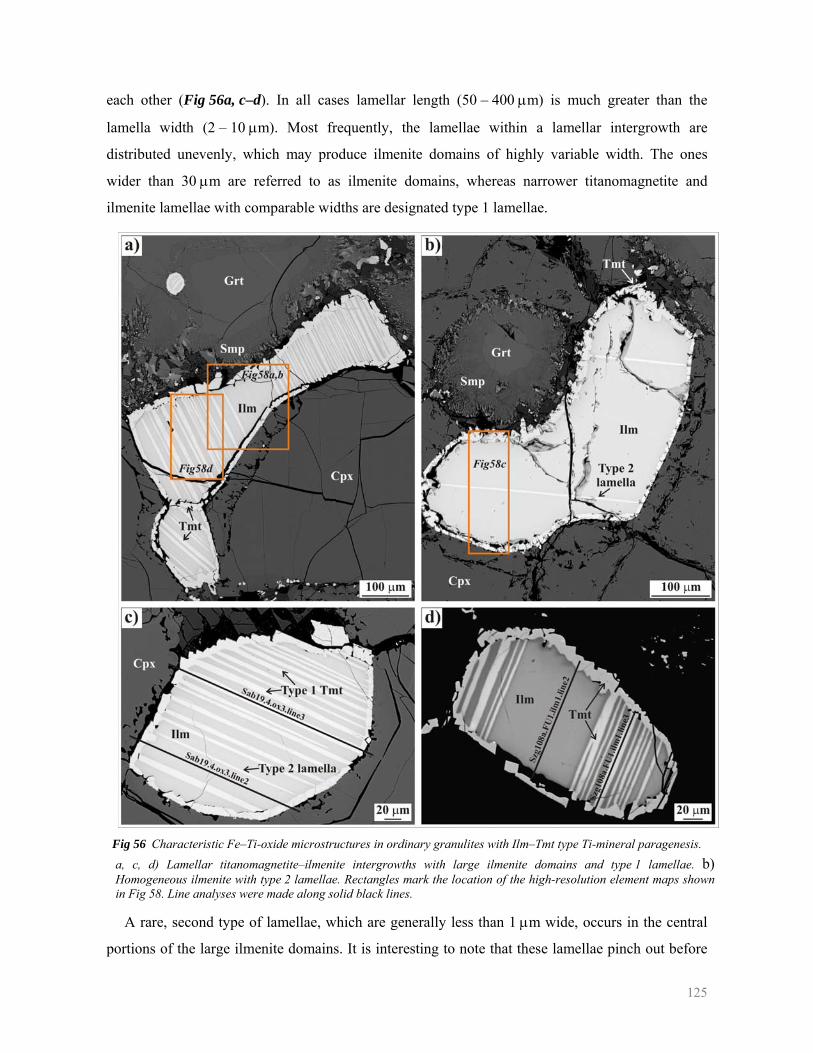
125
each other (Fig 56a, c–d). In all cases lamellar length (50 – 400 μm) is much greater than the
lamella width (2 – 10 μm). Most frequently, the lamellae within a lamellar intergrowth are
distributed unevenly, which may produce ilmenite domains of highly variable width. The ones
wider than 30 μm are referred to as ilmenite domains, whereas narrower titanomagnetite and
ilmenite lamellae with comparable widths are designated type 1 lamellae.
Fig 56 Characteristic Fe–Ti-oxide microstructures in ordinary granulites with Ilm–Tmt type Ti-mineral paragenesis. a, c, d) Lamellar titanomagnetite–ilmenite intergrowths with large ilmenite domains and type 1 lamellae. b) Homogeneous ilmenite with type 2 lamellae. Rectangles mark the location of the high-resolution element maps shown in Fig 58. Line analyses were made along solid black lines.
A rare, second type of lamellae, which are generally less than 1 μm wide, occurs in the central
portions of the large ilmenite domains. It is interesting to note that these lamellae pinch out before
126
they reach the ilmenite grain boundary at the interface with the titanomagnetite corona (Fig 56d).
We refer to this microstructure as type 2 lamellae. Although type 2 lamellae are generally too
narrow to be analyzed by EMP, the trends observed in the element maps suggest that these lamellae
are rich in Al and Fe.
Homogeneous ilmenite grains (Fig 56b) are less frequent than lamellar titanomagnetite–ilmenite
intergrowths. Usually, they are rounded in shape both as inclusions and in the matrix. They often
contain small lamellae of less than one micron width (Fig 56b). These lamellae are oriented and
comprise only a few volume percent of the ilmenite grain. In many cases, these lamellae do not
reach the rims of the ilmenite grain but tail off close to the titanomagnetite corona. Based on their
striking similarity to type 2 lamellae in the lamellar intergrowths, this microstructure is also
referred to as type 2 lamellae.
VII.1.2 Oxide mineral chemistry
Titanomagnetite in both samples contains Fe, Ti, Al, and Mg along with minor Mn and Cr.
Representative analyses of titanomagnetite in different microstructural positions are shown in
Table 10 together with titanomagnetite compositions measured in the groundmass of the alkali
basalt from Hegyestű (KÓTHAY et al. 2005). The titanomagnetite corona is similar in composition
to titanomagnetite grains from the host basalt. Both are rich in Al2O3 and MgO compared to type 1
titanomagnetite lamellae. Titanomagnetite solid solutions were recalculated in terms of magnetite
and ulvospinel, utilizing the method of STORMER (1983). These compositions are plotted on a Fe–
Ti–O ternary diagram (Fig 57). While the ulvospinel content of the titanomagnetite corona is
different for the two samples, it is quite consistent within one xenolith (Fig 57). Type 1
titanomagnetite lamellae always have a lower ulvospinel content than the corona, and thin
(d < 5 μm) lamellae always have higher ulvospinel contents than the thicker ones (see Fig 57 and
Table 10). The composition of type 2 lamellae could not be analyzed quantitatively because of their
small size. However, high-resolution line analysis indicates that they are most likely Al-bearing
titanomagnetites.
Ilmenite forms a solid solution with hematite, but in some cases it also contains remarkably high
Mg and some Al (Table 11). The MgO content varies between 2 – 5.5 wt%, while Al2O3
concentrations rarely exceed 1 wt%. A set of ilmenite analyses, with a hematite component, is
shown in the Fe–Ti–O ternary diagram (Fig 57). Hemo-ilmenite solid solutions were recalculated
in terms of hematite and ilmenite, utilizing the method of STORMER (1983). Here, core analyses
from the homogeneous ilmenite grains and large ilmenite domains from the lamellar
titanomagnetite–ilmenite intergrowths, plot in the same place. The edges of these grains close to the
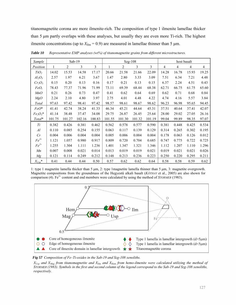
127
titanomagnetite corona are more ilmenite-rich. The composition of type 1 ilmenite lamellae thicker
than 5 μm partly overlaps with these analyses, but usually they are even more Ti-rich. The highest
ilmenite concentrations (up to XIlm = 0.9) are measured in lamellae thinner than 5 μm.
Table 10 Representative EMP analyses (wt%) of titanomagnetite grains from different microstructures.
Sample Sab-19 Szg-108 host basalt Position 1 2 3 3 1 2 3 3 4 4 4 4
TiO2 14.02 15.53 14.58 17.17 20.66 21.58 21.66 22.09 14.28 16.78 15.93 19.25Al2O3 2.57 1.97 6.21 3.67 1.47 2.80 3.33 3.09 7.51 6.34 7.21 4.48 Cr2O3 0.15 0.20 0.13 0.16 0.17 0.21 0.13 0.15 6.37 2.24 4.51 0.43 FeOt 78.43 77.37 71.96 71.99 73.11 69.39 68.44 68.38 62.71 66.75 61.75 65.60MnO 0.21 0.26 0.73 0.47 0.41 0.62 0.64 0.69 0.62 0.71 0.68 0.84 MgO 2.24 2.10 4.80 3.97 2.75 4.01 4.48 4.22 4.74 4.16 5.57 3.84 Total 97.63 97.42 98.41 97.42 98.57 98.61 98.67 98.62 96.23 96.98 95.65 94.45FeO* 41.41 42.74 38.24 41.33 46.34 45.21 44.64 45.31 37.51 40.64 37.41 42.07
Fe2O3* 41.14 38.48 37.47 34.08 29.75 26.87 26.45 25.64 28.00 29.02 27.05 26.16Total* 101.75 101.27 102.16 100.83 101.55 101.30 101.32 101.19 99.04 99.89 98.35 97.07
Ti 0.382 0.426 0.381 0.462 0.562 0.578 0.577 0.590 0.381 0.448 0.425 0.534Al 0.110 0.085 0.254 0.155 0.063 0.117 0.139 0.129 0.314 0.265 0.302 0.195Cr 0.004 0.006 0.004 0.004 0.005 0.006 0.004 0.004 0.178 0.063 0.126 0.012
Fe3+ 1.121 1.057 0.980 0.917 0.809 0.720 0.704 0.685 0.747 0.775 0.722 0.725Fe2+ 1.255 1.304 1.111 1.236 1.401 1.347 1.321 1.346 1.112 1.207 1.110 1.296Mn 0.007 0.008 0.021 0.014 0.013 0.019 0.019 0.021 0.019 0.021 0.021 0.026Mg 0.121 0.114 0.249 0.212 0.148 0.213 0.236 0.223 0.250 0.220 0.295 0.211
XUsp* 0.41 0.44 0.44 0.50 0.57 0.62 0.62 0.64 0.58 0.58 0.59 0.62
1: type 1 magnetite lamella thicker than 5 μm, 2: type 1magnetite lamella thinner than 5 μm, 3: magnetite overgrowth. Magnetite compositions from the groundmass of the Hegyestű alkali basalt (KÓTHAY et al., 2005) are also shown for comparison (4). Fe3+ content and end members were calculated by using the method of STORMER (1983).
Fig 57 Composition of Fe–Ti-oxides in the Sab-19 and Szg-108 xenoliths. XUsp and XMag from titanomagnetite and XIlm and XHem from hemo-ilmenite were calculated utilizing the method of STORMER (1983). Symbols in the first and second column of the legend correspond to the Sab-19 and Szg-108 xenoliths, respectively.
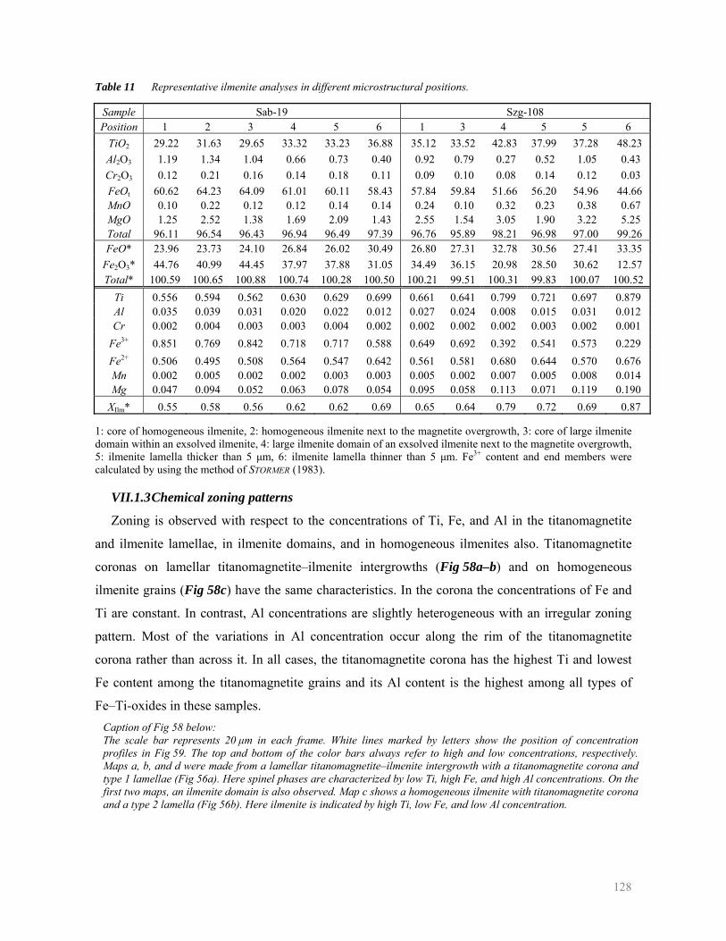
128
Table 11 Representative ilmenite analyses in different microstructural positions.
Sample Sab-19 Szg-108 Position 1 2 3 4 5 6 1 3 4 5 5 6
TiO2 29.22 31.63 29.65 33.32 33.23 36.88 35.12 33.52 42.83 37.99 37.28 48.23 Al2O3 1.19 1.34 1.04 0.66 0.73 0.40 0.92 0.79 0.27 0.52 1.05 0.43 Cr2O3 0.12 0.21 0.16 0.14 0.18 0.11 0.09 0.10 0.08 0.14 0.12 0.03 FeOt 60.62 64.23 64.09 61.01 60.11 58.43 57.84 59.84 51.66 56.20 54.96 44.66 MnO 0.10 0.22 0.12 0.12 0.14 0.14 0.24 0.10 0.32 0.23 0.38 0.67 MgO 1.25 2.52 1.38 1.69 2.09 1.43 2.55 1.54 3.05 1.90 3.22 5.25 Total 96.11 96.54 96.43 96.94 96.49 97.39 96.76 95.89 98.21 96.98 97.00 99.26 FeO* 23.96 23.73 24.10 26.84 26.02 30.49 26.80 27.31 32.78 30.56 27.41 33.35
Fe2O3* 44.76 40.99 44.45 37.97 37.88 31.05 34.49 36.15 20.98 28.50 30.62 12.57 Total* 100.59 100.65 100.88 100.74 100.28 100.50 100.21 99.51 100.31 99.83 100.07 100.52
Ti 0.556 0.594 0.562 0.630 0.629 0.699 0.661 0.641 0.799 0.721 0.697 0.879 Al 0.035 0.039 0.031 0.020 0.022 0.012 0.027 0.024 0.008 0.015 0.031 0.012 Cr 0.002 0.004 0.003 0.003 0.004 0.002 0.002 0.002 0.002 0.003 0.002 0.001
Fe3+ 0.851 0.769 0.842 0.718 0.717 0.588 0.649 0.692 0.392 0.541 0.573 0.229 Fe2+ 0.506 0.495 0.508 0.564 0.547 0.642 0.561 0.581 0.680 0.644 0.570 0.676 Mn 0.002 0.005 0.002 0.002 0.003 0.003 0.005 0.002 0.007 0.005 0.008 0.014 Mg 0.047 0.094 0.052 0.063 0.078 0.054 0.095 0.058 0.113 0.071 0.119 0.190
XIlm* 0.55 0.58 0.56 0.62 0.62 0.69 0.65 0.64 0.79 0.72 0.69 0.87
1: core of homogeneous ilmenite, 2: homogeneous ilmenite next to the magnetite overgrowth, 3: core of large ilmenite domain within an exsolved ilmenite, 4: large ilmenite domain of an exsolved ilmenite next to the magnetite overgrowth, 5: ilmenite lamella thicker than 5 μm, 6: ilmenite lamella thinner than 5 μm. Fe3+ content and end members were calculated by using the method of STORMER (1983).
VII.1.3 Chemical zoning patterns
Zoning is observed with respect to the concentrations of Ti, Fe, and Al in the titanomagnetite
and ilmenite lamellae, in ilmenite domains, and in homogeneous ilmenites also. Titanomagnetite
coronas on lamellar titanomagnetite–ilmenite intergrowths (Fig 58a–b) and on homogeneous
ilmenite grains (Fig 58c) have the same characteristics. In the corona the concentrations of Fe and
Ti are constant. In contrast, Al concentrations are slightly heterogeneous with an irregular zoning
pattern. Most of the variations in Al concentration occur along the rim of the titanomagnetite
corona rather than across it. In all cases, the titanomagnetite corona has the highest Ti and lowest
Fe content among the titanomagnetite grains and its Al content is the highest among all types of
Fe–Ti-oxides in these samples. Caption of Fig 58 below: The scale bar represents 20 μm in each frame. White lines marked by letters show the position of concentration profiles in Fig 59. The top and bottom of the color bars always refer to high and low concentrations, respectively. Maps a, b, and d were made from a lamellar titanomagnetite–ilmenite intergrowth with a titanomagnetite corona and type 1 lamellae (Fig 56a). Here spinel phases are characterized by low Ti, high Fe, and high Al concentrations. On the first two maps, an ilmenite domain is also observed. Map c shows a homogeneous ilmenite with titanomagnetite corona and a type 2 lamella (Fig 56b). Here ilmenite is indicated by high Ti, low Fe, and low Al concentration.
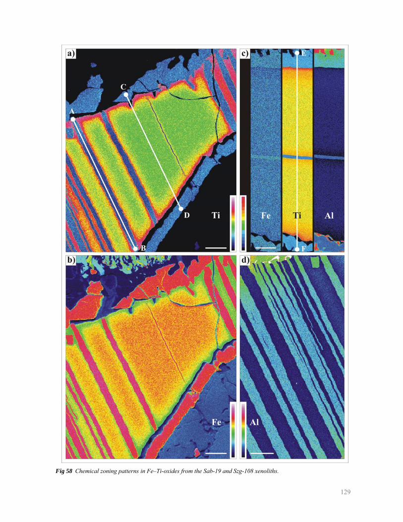
129
Fig 58 Chemical zoning patterns in Fe–Ti-oxides from the Sab-19 and Szg-108 xenoliths.
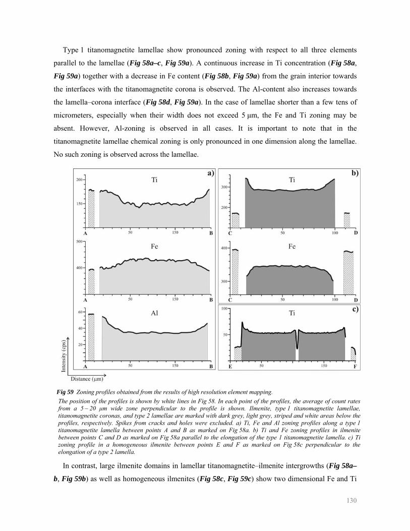
130
Type 1 titanomagnetite lamellae show pronounced zoning with respect to all three elements
parallel to the lamellae (Fig 58a–c, Fig 59a). A continuous increase in Ti concentration (Fig 58a,
Fig 59a) together with a decrease in Fe content (Fig 58b, Fig 59a) from the grain interior towards
the interfaces with the titanomagnetite corona is observed. The Al-content also increases towards
the lamella–corona interface (Fig 58d, Fig 59a). In the case of lamellae shorter than a few tens of
micrometers, especially when their width does not exceed 5 μm, the Fe and Ti zoning may be
absent. However, Al-zoning is observed in all cases. It is important to note that in the
titanomagnetite lamellae chemical zoning is only pronounced in one dimension along the lamellae.
No such zoning is observed across the lamellae.
Fig 59 Zoning profiles obtained from the results of high resolution element mapping. The position of the profiles is shown by white lines in Fig 58. In each point of the profiles, the average of count rates from a 5 – 20 μm wide zone perpendicular to the profile is shown. Ilmenite, type 1 titanomagnetite lamellae, titanomagnetite coronas, and type 2 lamellae are marked with dark grey, light grey, striped and white areas below the profiles, respectively. Spikes from cracks and holes were excluded. a) Ti, Fe and Al zoning profiles along a type 1 titanomagnetite lamella between points A and B as marked on Fig 58a. b) Ti and Fe zoning profiles in ilmenite between points C and D as marked on Fig 58a parallel to the elongation of the type 1 titanomagnetite lamella. c) Ti zoning profile in a homogeneous ilmenite between points E and F as marked on Fig 58c perpendicular to the elongation of a type 2 lamella.
In contrast, large ilmenite domains in lamellar titanomagnetite–ilmenite intergrowths (Fig 58a–
b, Fig 59b) as well as homogeneous ilmenites (Fig 58c, Fig 59c) show two dimensional Fe and Ti
131
zoning patterns. The central part of these ilmenite grains show homogeneous compositions with the
lowest Ti and highest Fe concentrations. The Ti concentrations increase while the Fe contents
decrease in the ilmenite when approaching the interface with the titanomagnetite corona (Fig 58a,
Fig 59b–c). In the case of the ilmenite domains, an increase in the Ti and decrease in the Fe
concentration is also observable towards the interface with type 1 titanomagnetite lamellae. The
width of high Ti concentration zones in the ilmenite successively decreases with increasing distance
from the ilmenite – titanomagnetite corona – type 1 titanomagnetite lamella triple junctions. On the
other hand, the width of this zone is constant in homogeneous ilmenites. Although Al
concentrations are very low in the ilmenite domains and in the homogeneous ilmenites, depletion in
Al is observable in both cases at the ilmenite – titanomagnetite corona interface and at the ilmenite
– type 2 lamella interface. The Al-depletion is more pronounced in the latter case, which results in
characteristically asymmetric Al patterns (see Fig 58c).
The cores of type 1 ilmenite lamellae have higher Ti and lower Fe concentrations than the larger
ilmenite domains and homogeneous ilmenites. In relatively short and/or thin ilmenite lamellae the
Ti content is systematically higher than in wider lamellae (Fig 58a). Enrichment in Ti and
depletion in Fe close to the titanomagnetite corona also occurs in type 1 ilmenite lamellae, but in
this case the enrichment and depletion trends are not as prominent as in other types of ilmenite
(Fig 58a–b). In some ilmenite lamellae thinner than 5 μm, the Fe and Ti zoning pattern is absent
and the Fe and Ti concentrations correspond to the composition of the high Ti zone at the ilmenite
– titanomagnetite corona interface. The Al contents of the ilmenite lamellae are generally lower
than in the large ilmenite domains or homogeneous ilmenite grains. Aluminum zoning is not
observed in type 1 ilmenite lamellae.
VII.2 Thermodynamic analysis of Fe–Ti-oxide microstructures
VII.2.1 Phase relations in the Fe–Ti–O system
In the Fe–Ti–O system, three Fe–Ti-oxide solid solution series exist. These include the
titanomagnetite solid solution between magnetite and ulvospinel, the hemo-ilmenite solid solution
between hematite and ilmenite, and the pseudobrookite solid solution between ferrous
pseudobrookite and pure pseudobrookite. A recent update, regarding the phase relations between
these solid solutions, has been described in detail by LATTARD et al. (2005). Only the most
important features of the first two solid solution series are described here. These play an important
role in the interpretation of the observed microstructures and chemical zoning patterns.
Chemographic phase diagrams were constructed for the Fe–Ti–O system using the PERPLEX
software (CONNOLLY 1990). Thermodynamic data were taken from HOLLAND and POWELL (1998)
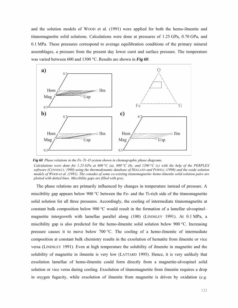
132
and the solution models of WOOD et al. (1991) were applied for both the hemo-ilmenite and
titanomagnetite solid solutions. Calculations were done at pressures of 1.25 GPa, 0.70 GPa, and
0.1 MPa. These pressures correspond to average equilibration conditions of the primary mineral
assemblages, a pressure from the present day lower curst and surface pressure. The temperature
was varied between 600 and 1300 °C. Results are shown in Fig 60.
Fig 60 Phase relations in the Fe–Ti–O system shown in chemographic phase diagrams. Calculations were done for 1.25 GPa at 600 °C (a), 800 °C (b), and 1200 °C (c) with the help of the PERPLEX software (CONNOLLY, 1990) using the thermodynamic database of HOLLAND and POWELL (1998) and the oxide solution models of WOOD et al. (1991). The conodes of some co-existing titanomagnetite–hemo-ilmenite solid solution pairs are plotted with dotted lines. Miscibility gaps are filled with grey.
The phase relations are primarily influenced by changes in temperature instead of pressure. A
miscibility gap appears below 900 °C between the Fe- and the Ti-rich side of the titanomagnetite
solid solution for all three pressures. Accordingly, the cooling of intermediate titanomagnetite at
constant bulk composition below 900 °C would result in the formation of a lamellar ulvospinel–
magnetite intergrowth with lamellae parallel along (100) (LINDSLEY 1991). At 0.1 MPa, a
miscibility gap is also predicted for the hemo-ilmenite solid solution below 900 °C. Increasing
pressure causes it to move below 700 °C. The cooling of a hemo-ilmenite of intermediate
composition at constant bulk chemistry results in the exsolution of hematite from ilmenite or vice
versa (LINDSLEY 1991). Even at high temperature the solubility of ilmenite in magnetite and the
solubility of magnetite in ilmenite is very low (LATTARD 1995). Hence, it is very unlikely that
exsolution lamellae of hemo-ilmenite could form directly from a magnetite-ulvospinel solid
solution or vice versa during cooling. Exsolution of titanomagnetite from ilmenite requires a drop
in oxygen fugacity, while exsolution of ilmenite from magnetite is driven by oxidation (e.g.
133
LINDSLEY 1962, 1963; BUDDINGTON and LINDSLEY 1964, SIMONS and WOERMANN 1978; SPENCER
and LINDSLEY 1978; HAMMOND et al. 1982; ANDERSEN and LINDSLEY 1988, LATTARD et al. 2005).
The Fe–Ti partitioning between coexisting hemo-ilmenite and titanomagnetite solid solutions is
temperature dependent. Upon cooling the composition of the ilmenite successively shifts towards
the pure ilmenite and the composition of titanomagnetite shifts towards pure magnetite.
VII.2.2 Evolution of Fe–Ti-oxides
According to petrographic observations, the lamellar titanomagnetite–ilmenite intergrowths had
a homogeneous precursor phase, which presumably was in microstructural equilibrium with the
other phases of the primary mineral assemblage. This was then followed by the formation of type 1
titanomagnetite and ilmenite lamellae due to exsolution induced by a change in oxygen fugacity.
Since the composition of the homogeneous ilmenite grains corresponds to the core of the large
ilmenite domains and wide (d > 20 μm) type 1 ilmenite lamellae, it is likely that the formation of
type 1 titanomagnetite and ilmenite lamellae and the crystallization of the homogeneous ilmenites
took place at the same time. Both oxide types then experienced subsequent overgrowth of a
titanomagnetite corona. The striking similarities between the composition of the titanomagnetite
corona and titanomagnetite grains in the groundmass of the host basalt (Table 10) strongly suggest
that the titanomagnetite coronas were formed during xenolith – host basalt interaction. Chemical
zoning patterns, especially Al-zoning in type 1 titanomagnetite lamellae (Fig 59a), suggest that
overgrowth of titanomagnetite induced the chemical overprinting of both the homogeneous ilmenite
grains and the titanomagnetite–ilmenite intergrowths. This indicates that the type 1 titanomagnetite
and ilmenite lamellae were exsolved from a homogeneous precursor phase before the overgrowth
of the titanomagnetite coronas. The formation of trellis-type Ti-rich and Ti-poor titanomagnetite
(HAGGERTY 1991) from the titanomagnetite coronas on titanomagnetite–ilmenite intergrowths in
xenoliths from Kapolcs (Áldozó-tető) (Fig 28f) can be interpreted as a cooling phenomenon after
the volcanic uplift of the xenoliths to the surface. The fact that this type of mineral reaction is
restricted to xenoliths hosted by lava flows suggests that the cooling rate of tuff-hosted xenoliths is
significantly higher.
The formation of type 2 exsolution lamellae cannot be fitted into the above mentioned oxide
evolution on the basis of petrographic information. The Al pattern in ilmenite shown in Fig 58c
suggests that somewhat more Al was extracted by the type 2 lamellae than by the titanomagnetite
corona. This could be explained in two ways. First, formation of type 2 lamellae could have
occurred before the xenolith – host basalt interaction or the type 2 lamellae are a more effective
134
sink of Al, than the titanomagnetite corona. Both processes are possible, and could have acted at the
same time.
VII.2.3 Oxide thermometry and oxygen barometry
The compositions of coexisting titanomagnetite and ilmenite are temperature-dependent. The
determination of the conditions at which type 1 titanomagnetite lamellae exsolved from ilmenite is
difficult, because their composition has been modified by the xenolith – host basalt interaction as
indicated by the Fe, Ti, and Al zoning patterns (Fig 58, Fig 59). I used the compositions of the core
regions of the widest titanomagnetite and ilmenite lamellae in the geothermobarometric
calculations (see Fig 61a). Some conodes are also shown, which link the compositions of
titanomagnetite–ilmenite pairs in equilibrium at 1.25 GPa, 1000 °C (formation conditions of
primary mineral assemblages) and 0.70 GPa, 1100 °C (possible conditions after basin extension).
These titanomagnetite and ilmenite lamella compositions cannot coexist in equilibrium in either
condition. Due to cation exchange with the titanomagnetite corona during xenolith – host basalt
interaction, all titanomagnetite as well as the thin ilmenite lamellae have lost their ‘memory’ of the
granulite facies stage of metamorphism. Hence, they cannot be used to estimate the conditions
under which they formed. Application of the thermometer of GHIORSO and EVANS (2008) for these
pairs yields unrealistically high temperatures in excess of 1400 °C indicating that equilibrium
compositions were not preserved.
On the basis of the chemical zoning patterns, it is likely that the homogeneous core region of the
ilmenite domains have preserved the ilmenite composition that was attained during the exsolution
of type 1 lamellae. Most likely, the formation of type 1 titanomagnetite and ilmenite lamellae took
place during the formation of the primary mineral assemblage in the deep crust at temperatures of
1000 to 1100 °C. I calculated the composition of type 1 titanomagnetite lamellae, which are in
equilibrium with the cores of large ilmenite domains at these temperatures using the Gibbs free
energy minimization technique in conjunction with the oxide solution model of WOOD et al. (1991)
(see chemographic phase diagram in Fig 61) and the magnetite–ilmenite thermometers of GHIORSO
and EVANS (2008) and of SAUERZAPF et al. (2008). According to the phase diagram in Fig 61, the
core of ilmenite domains in lamellar titanomagnetite–ilmenite intergrowths from the two xenoliths
(XIlm = 0.56 for the Sab-19 and XIlm = 0.64 for the Szg-108 xenolith) would coexist with a
magnetite-rich titanomagnetite phase (XUsp = 0.06 for Sab-19 and XUsp = 0.11 for Szg-108) at the
equilibration temperature of the primary mineral assemblage (1000 °C). Application of the
magnetite–ilmenite thermometers of GHIORSO and EVANS (2008) (XUsp = 0.25 for Sab-19 and
XUsp = 0.30 for Szg-108) and SAUERZAPF et al. (2008) (XUsp = 0.12 for Sab-19 and XUsp = 0.19 for
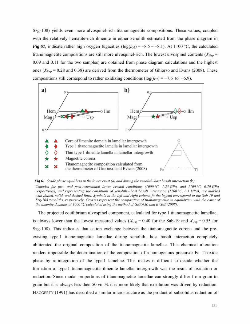
135
Szg-108) yields even more ulvospinel-rich titanomagnetite compositions. These values, coupled
with the relatively hematite-rich ilmenite in either xenolith estimated from the phase diagram in
Fig 61, indicate rather high oxygen fugacities (log(fO2) = −8.5 – −8.1). At 1100 °C, the calculated
titanomagnetite compositions are still more ulvospinel-rich. The lowest ulvospinel contents (XUsp =
0.09 and 0.11 for the two samples) are obtained from phase diagram calculations and the highest
ones (XUsp = 0.28 and 0.38) are derived from the thermometer of Ghiorso and Evans (2008). These
compositions still correspond to rather oxidizing conditions (log(fO2) = −7.6 to −6.9).
Fig 61 Oxide phase equilibria in the lower crust (a) and during the xenolith–host basalt interaction (b). Conodes for pre- and post-extensional lower crustal conditions (1000 °C, 1.25 GPa, and 1100 °C, 0.70 GPa, respectively), and representing the conditions of xenolith – host basalt interaction (1200 °C, 0.1 MPa), are marked with dotted, solid, and dashed lines. Symbols in the left and right column fo the legend correspond to the Sab-19 and Szg-108 xenoliths, respectively. Crosses represent the composition of titanomagnetite in equilibrium with the cores of the ilmenite domains at 1000 °C calculated using the method of GHIORSO and EVANS (2008).
The projected equilibrium ulvospinel component, calculated for type 1 titanomagnetite lamellae,
is always lower than the lowest measured values (XUsp = 0.40 for the Sab-19 and XUsp = 0.55 for
Szg-108). This indicates that cation exchange between the titanomagnetite corona and the pre-
existing type 1 titanomagnetite lamellae during xenolith – host basalt interaction completely
obliterated the original composition of the titanomagnetite lamellae. This chemical alteration
renders impossible the determination of the composition of a homogenous precursor Fe–Ti-oxide
phase by re-integration of the type 1 lamellae. This makes it difficult to decide whether the
formation of type 1 titanomagnetite–ilmenite lamellar intergrowth was the result of oxidation or
reduction. Since modal proportions of titanomagnetite lamellae can strongly differ from grain to
grain but it is always less then 50 vol.% it is more likely that exsolution was driven by reduction.
HAGGERTY (1991) has described a similar microstructure as the product of subsolidus reduction of
136
ilmenite. The lack of an ilmenite trellis structure (HAGGERTY 1991) also supports the hypothesis
that type 1 exsolution lamellae were not formed by the oxidation of ulvospinel-rich titanomagnetite
(HARLOV 2000; HARLOV and HANSEN 2005).
The formation of the titanomagnetite corona is clearly the result of xenolith – host basalt
interaction. This titanomagnetite corona was not in chemical equilibrium with the pre-existing
titanomagnetite lamellae at the temperatures of xenolith – host basalt interaction. This induced the
formation of chemical zoning patterns in the Fe–Ti-oxides. Temperature estimations according to
the thermometer of GHIORSO and EVANS (2008) for titanomagnetite corona – ilmenite analysis pairs
right at the interface yielded 1200 ± 30 °C, which corresponds to the temperature of the host basalt.
The oxygen fugacity values calculated for these pairs are between log(fO2) = −6.6 to −6.1, which
also correspond to the oxygen fugacity of the host basalt. This indicates that the ilmenite has
reached equilibrium with the titanomagnetite corona at the immediate contact.
VII.3 Diffusion modelling
VII.3.1 Formation of chemical zoning patterns
Systematic chemical zoning along the titanomagnetite lamellae and within the ilmenite host
towards the interfaces with the titanomagnetite corona (Fig 58, Fig 59), can be explained by cation
exchange. The rate and extent was controlled by solid state diffusion. In the case of type 1
titanomagnetite lamellae, this led to the introduction of Ti, Al, and Mg from the titanomagnetite
corona from both sides towards the central portions of the grains, while Fe diffused outwards into
the titanomagnetite corona. Since compositional variations in the titanomagnetite lamellae were
observed only along the lamellae and not in the direction perpendicular to the lamellae, diffusion
may be considered as one-dimensional. The Ti-rich zone observed in the homogeneous ilmenites
and in the ilmenite domains along the interface with the titanomagnetite corona reflects limited Fe–
Ti exchange between the titanomagnetite corona and the ilmenite grains. This is strengthened by
the argument that the ilmenite compositions measured right at the interface correspond to those
which would form if the ilmenite was in equilibrium with the titanomagnetite corona at 1200 °C. In
homogeneous ilmenite grains and in ilmenite domains far from the type 1 titanomagnetite lamellae,
the development of the Ti-rich zone should be controlled by volume diffusion in ilmenite. The
widening of the Ti-rich zone at triple junctions of the titanomagnetite corona, ilmenite domains,
and type 1 titanomagnetite lamellae may be due to the role of grain boundary diffusion along the
titanomagnetite lamella – ilmenite interface. Another possible explanation is that Fe–Ti exchange
also takes place along the lamella interface between the chemically modified type 1 titanomagnetite
lamellae and the ilmenite domains, which have preserved the compositions that they attained during
137
formation of the titanomagnetite lamellae. This is supported by the fact that Ti concentrations in
ilmenite along this interface are lower than along the ilmenite – titanomagnetite corona interface.
VII.3.2 Duration of xenolith – host basalt interaction
The development of compositional profiles in the studied Fe–Ti-oxides was induced during the
crystallization of the titanomagnetite corona, which could be regarded as the principal chemical
interaction between the xenolith and the host basalt. Since the xenoliths were hosted in basaltic
tuffs, it is very likely that the quenching of the system was very rapid after reaching the surface,
effectively halting solid state diffusion. As a consequence, the duration of xenolith – host basalt
interaction can be determined by modeling the chemical zoning in type 1 titanomagnetite lamellae.
The compositional changes were approximated by the exchange of the magnetite and ulvospinel
components, as the result of the coupled exchange: 2 Fe3+ ↔ Fe2+ + Ti4+, because the correlation
between the decrease in the Fe and the increase in the Ti concentration is very strong (Fig 59a) and
all other components together usually do not give more than 5 wt% of the oxide composition. The
results of line analyses along type 1 titanomagnetite lamellae were evaluated and used for
modeling. An example of an evaluated profile is shown in Fig 62a. We derived the ulvospinel mole
fraction (XUsp) from the measured data by utilizing the method of STORMER (1983), which also
takes into account the presence of minor components. We presume that the titanomagnetite corona
served as a source of ulvospinel component to the type 1 titanomagnetite lamellae on both sides and
that element migration took place dominantly perpendicular to the type 1 titanomagnetite lamella –
titanomagnetite corona interface by solid state volume diffusion. Some ulvospinel component may
have been extracted from the titanomagnetite lamellae due to Fe–Ti exchange between the type 1
titanomagnetite lamellae, and the ilmenite host. This effect is, however, deemed to be subordinate
and diffusion along the type 1 titanomagnetite lamellae was regarded as one-dimensional.
According to numerous diffusion experiments in titanomagnetite grains of different composition
under various conditions (e.g. DIECKMANN and SCHMALZRIED 1977; FREER and HAUPTMAN 1978;
FREER 1980; PRICE 1981; ARAGON et al. 1984; AGGARWAL et al. 1997; DIECKMANN 1998;
AGGARWAL and DIECKMANN 2002), cation diffusion in titanomagnetite is principally influenced by
three factors: temperature, oxygen fugacity, and ulvospinel content. Since the edge of the ilmenite
grains appear to be in equilibrium with the titanomagnetite corona at the interface at 1200 °C and
log(fO2) = −6.5 to −6.1, which corresponds, within error, to the temperature and oxygen fugacity of
the host basalt, i.e. 1220 – 1270 °C and log(fO2) = −6.6 to −6.5, both parameters can be treated as
constant. The compositional dependence of Fe, Ti, Mn, and Co tracer diffusion coefficients have
been studied systematically by AGGARWAL and DIECKMANN (2002) at temperatures of 1100 –
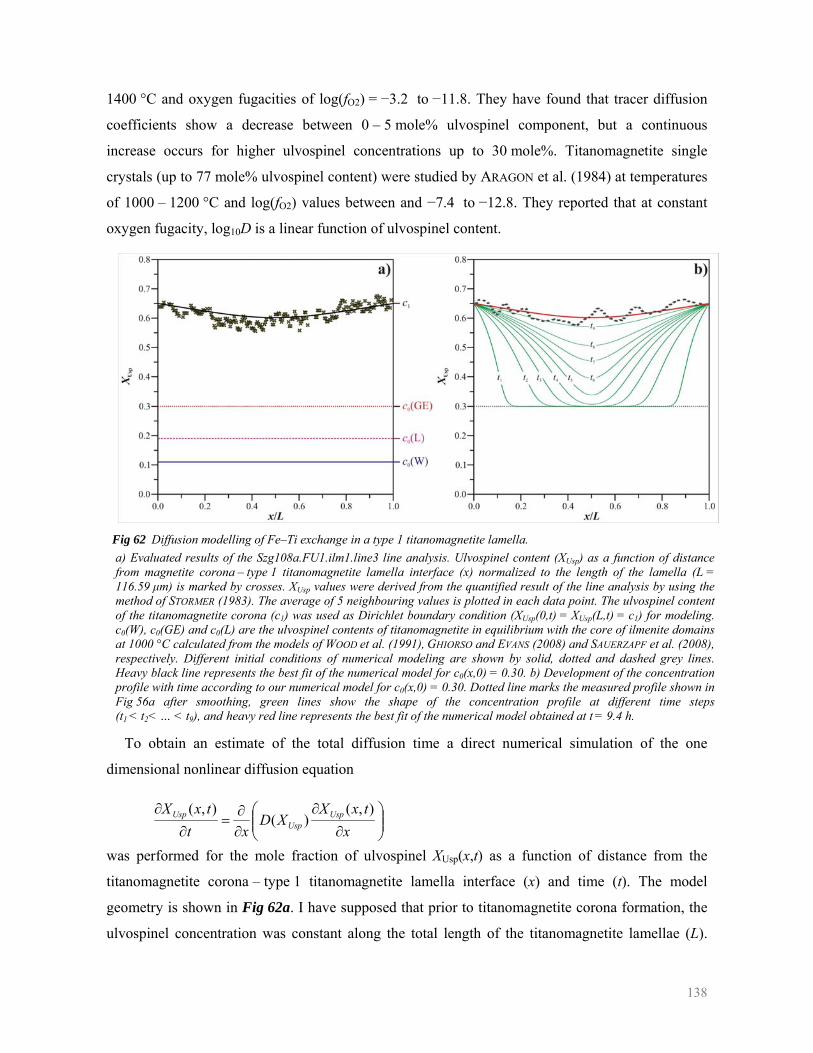
138
1400 °C and oxygen fugacities of log(fO2) = −3.2 to −11.8. They have found that tracer diffusion
coefficients show a decrease between 0 – 5 mole% ulvospinel component, but a continuous
increase occurs for higher ulvospinel concentrations up to 30 mole%. Titanomagnetite single
crystals (up to 77 mole% ulvospinel content) were studied by ARAGON et al. (1984) at temperatures
of 1000 – 1200 °C and log(fO2) values between and −7.4 to −12.8. They reported that at constant
oxygen fugacity, log10D is a linear function of ulvospinel content.
Fig 62 Diffusion modelling of Fe–Ti exchange in a type 1 titanomagnetite lamella. a) Evaluated results of the Szg108a.FU1.ilm1.line3 line analysis. Ulvospinel content (XUsp) as a function of distance from magnetite corona – type 1 titanomagnetite lamella interface (x) normalized to the length of the lamella (L = 116.59 μm) is marked by crosses. XUsp values were derived from the quantified result of the line analysis by using the method of STORMER (1983). The average of 5 neighbouring values is plotted in each data point. The ulvospinel content of the titanomagnetite corona (c1) was used as Dirichlet boundary condition (XUsp(0,t) = XUsp(L,t) = c1) for modeling. c0(W), c0(GE) and c0(L) are the ulvospinel contents of titanomagnetite in equilibrium with the core of ilmenite domains at 1000 °C calculated from the models of WOOD et al. (1991), GHIORSO and EVANS (2008) and SAUERZAPF et al. (2008), respectively. Different initial conditions of numerical modeling are shown by solid, dotted and dashed grey lines. Heavy black line represents the best fit of the numerical model for c0(x,0) = 0.30. b) Development of the concentration profile with time according to our numerical model for c0(x,0) = 0.30. Dotted line marks the measured profile shown in Fig 56a after smoothing, green lines show the shape of the concentration profile at different time steps (t1 < t2< … < t9), and heavy red line represents the best fit of the numerical model obtained at t = 9.4 h.
To obtain an estimate of the total diffusion time a direct numerical simulation of the one
dimensional nonlinear diffusion equation
⎟⎟⎠
⎞⎜⎜⎝
⎛∂
∂∂∂
=∂
∂x
txXXD
xttxX Usp
UspUsp ),(
)(),(
was performed for the mole fraction of ulvospinel XUsp(x,t) as a function of distance from the
titanomagnetite corona – type 1 titanomagnetite lamella interface (x) and time (t). The model
geometry is shown in Fig 62a. I have supposed that prior to titanomagnetite corona formation, the
ulvospinel concentration was constant along the total length of the titanomagnetite lamellae (L).
139
The initial ulvospinel concentration (c0) was estimated from the core composition of ilmenite
domains assuming equilibrium Fe–Ti partitioning between titanomagnetite and ilmenite at 1000 or
1100 °C, where the thermodynamic models of WOOD et al. (1991), GHIORSO and EVANS (2008),
and SAUERZAPF et al. (2008) were used. We also assumed that the composition of the
titanomagnetite corona (c1) was buffered by the host basalt. For this reason, the solution was
calculated on the space interval Lx <<0 by using Dirichlet boundary conditions:
1),(),0( ctLXtX UspUsp == . The Fe–Ti interdiffusion coefficient (D(XUsp)), as a function of the
ulvospinel content, was approximated from the expression of ARAGON et al. (1984), UspXD ⋅+−= 140.393.1010 cm2/s, at 1200 °C and log(fO2) = −7.4. The oxygen fugacity for which the
compositional dependence of the diffusion coefficient was derived is 0.8 log unit lower than the
one estimated from the host basalt. However, these were the most oxidizing experimental
conditions obtained by ARAGON et al. (1984). According to AGGARWAL and DIECKMANN (2002),
cation diffusion coefficients in the titanomagnetite solid solution series show a minimum as a
function of oxygen fugacity due to a change in the diffusion mechanism. A correction due to the
oxygen fugacity difference could have been taken into account only if the tracer diffusion
coefficients for Fe and Ti in titanomagnetite were known for ulvospinel contents between 40 –
65 mole%. Since the most Ti-rich titanomagnetites in the systematic experiments of AGGARWAL
and DIECKMANN (2002) contain 10 – 35 mole% less ulvospinel, the extrapolation from these results
would lead to big uncertainties.
The development of the concentration profile with time is shown in Fig 62b. At each time step
deviations from the numerical solution and the observed titanomagnetite compositions was
calculated. The best fit was determined by minimizing the sum of the squared deviations (see
Fig 62b). By utilizing these approximations, the times estimated from the solution of the diffusion
equation vary between 9 – 20 hours for all profiles. The results are mainly influenced by the
estimate of the initial ulvospinel content of the titanomagnetite lamellae (c0). A change of c0 from
the highest value to the lowest increases the time estimate by a factor of ca. 1.5. These results are in
a reasonable agreement with the estimated magma ascent times as determined by SZABÓ and
BODNAR (1996). This suggests that the chemical overprint of the xenolith by the host basalt is
extremely fast.
Diffusion profiles in the ilmenite grains and domains were induced by the same event as the
ones in the type 1 titanomagnetite lamellae. Since the penetration depth of Ti in ilmenite rarely
exceeds 10 μm, which is at least one order of magnitude lower than in the type 1 titanomagnetite
lamellae, the Fe–Ti interdiffusion coefficient in ilmenite is significantly lower than in

140
titanomagnetite. Sluggish diffusion rates in ilmenite suggest that even if Fe–Ti exchange occurred
between the type 1 titanomagnetite and ilmenite lamellae, the extraction of Ti from the
titanomagnetite lamellae was not significant compared to the introduction of Ti from the
titanomagnetite corona.
141
VIII METAMORPHIC EVOLUTION OF THE XENOLITHS
By the combination of petrography, mineral chemistry, formation conditions of different mineral
assemblages and the results of thermodynamic and diffusion modelling of mineral reactions, the
metamorphic evolution of the studied mafic lower crustal xenoliths from the BBHVF was
constructed. It is in clear connection with tectonometamorphic processes acting in the lower crust.
However, the processes observed on the surface and in the lower curst are of different nature.
While extension in the upper crust and on the surface is generally manifested in brittle deformation,
the main deformation style in the lower crust is ductile. In addition, direct aging methods are hardly
applicable for rocks originating from the lower crust because of the high temperature. For these
reasons, the correlation of surface tectonics and lower crustal evolution is limited to large-scale
processes such as the extension of the lithosphere.
Considering the tectonic evolution of the Pannonian Basin, the metamorphic evolution of the
studied xenoliths is divided in three main stages. Primary mineral assemblages of the xenoliths
characterize the lower crust prior to the extension of the Pannonian Basin. Part of the reaction
microstructures are remnants of processes acting during the Miocene basin extension associated
with significant lithosphere thinning (e.g. STEGENA et al. 1975; HORVÁTH 1993; HUISMANS et al.
2001), whereas other reaction microstructures were formed during the interaction of the xenoliths
with the host basalt.
Primary mineral assemblages of the studied xenoliths are not uniform either in mineralogy or in
chemical composition. Based on mineral chemical characteristics they can be classified to five
xenolith types: ‘ordinary’ (Grt – Cpx – Pl ± Opx ± Amp ± Ilm ± Rt), Ca-rich (Grt – Cpx ± Pl ± Opx
± Amp ± Ttn), Mg-rich (Grt – Cpx – Pl – Opx ± Bt ± Rt ± Qtz) and Fe-rich granulites (Grt – Cpx –
Pl ± Amp ± Ilm) and low Ca rocks (Grt – Pl – Qtz ± Opx ± Bt ± Rt) (Section IV.3). Phase diagram
pseudosections (Fig 45) have shown that, although the bulk compositions of the different xenolith
types are different, all primary mineral assemblages are stable at pressures well above the pressure
of the present day Moho beneath the studied area. Regarding the tectonic evolution of the
Pannonian Basin, primary mineral assemblages were formed prior to the extension of the basin as it
was stated earlier by EMBEY-ISZTIN et al. (2003). The equilibration pressure and temperature of 52
studied mafic lower crustal xenoliths (between 1.0–1.6 GPa, 720–1070 °C, Fig 63) suggests that a
complete lower crustal section between 35 and 57 km depths (calculating with 2.8 g/cm3 crustal
density) was sampled by the host basalt. The estimated equilibration conditions partly overlap with
the formation pressure and temperature of the mafic granulites studied by EMBEY-ISZTIN et al.
142
(2003) (1.0–1.4 GPa and 800–1000 °C), but some xenoliths studied in this work formed at higher
pressures. The strong correlation of equilibration pressures and temperatures gives a rise to
construct the paleogeotherm of the Alpine orogenic root with 15 °C/km geothermal gradient
(Fig 48). At this stage of the metamorphic evolution the crust–mantle boundary was close to 60 km
depth and the temperature at the Moho reached 1100 °C. This implies that the thickness of the
Alpine orogenic root prior to the extension of the Pannonian Basin was similar to the orogenic root
of the present day Andes (Moho depth = 50–75 km, YUAN et al. 2000) or Himalayas (Moho
depth > 70 km, YUAN et al. 1997). The distribution of xenolith types with different bulk chemistry
within this orogenic root is completely random (Fig 63). Xenoliths with totally different bulk rock
compositions are equilibrated at the same pressure and temperature. Sometimes xenolith zones of
different rock types are alternating within a few centimeters (Fig 13b). This implies that very small
scale lateral inhomogeneities existed in the Alpine orogenic root prior to the formation of the
Pannonian Basin. This kind of heterogeneity is in good correspondance to the thermal and
rheological structure of a lower crust reworked during Andes-type subduction (e.g. FACCENDA et al.
2008).
Lateral heterogeneities in the lower crust further developed during the Miocene extension of the
Pannonian Basin. Probably the first mineralogical change induced by this tectonic event in the
lower crust was the type 1 breakdown of biotite. Basically restitic Grt–Opx–Pl mineral assemblages
(Fig 23b) were formed in the reaction, but rarely ocurring melt inclusions and K-feldspar
(Fig 23a–b) imply that significant amount of partial melt was separated from the restitic solid
phases. Grt–Opx–Pl mineral assemblages produced in the reaction equilibrated at (920–940 °C,
1.2–1.3 GPa). However, this equilibration temperature is below the experimentally determined
melting point of biotite (1000 °C at 1.2 GPa, NAIR and CHACKO 2002, Fig 44). According to
experimental constraints on biotite stability (Fig 44), the presence of CO2-rich fluids, as observed
in the rock, may significantly reduce the melting point of biotite (PETERSON and NEWTON 1990).
This suggests that fluid infiltration was an important driving force of biotite breakdown. In
addition, equilibration conditions of the reaction products correspond to the formation conditions of
primary mineral assemblages within the same xenolith (930–950 °C, 1.2–1.3 GPa in the Mi-63
xenolith), which reflects that biotite melting did not require significant heating.
On the basis of Ca-zoning in non-equilibrium garnets found in Opx–Grt granulites between a
low Ca rock and a Cpx–Opx–Grt granulite in the Mi-10 xenolith (Fig 30), at least part of the Opx–
Grt granulites were formed during such a partial melting event. Since the equilibration pressure and
temperature of these rocks corresponds well to the paleogeotherm, this partial melting event most
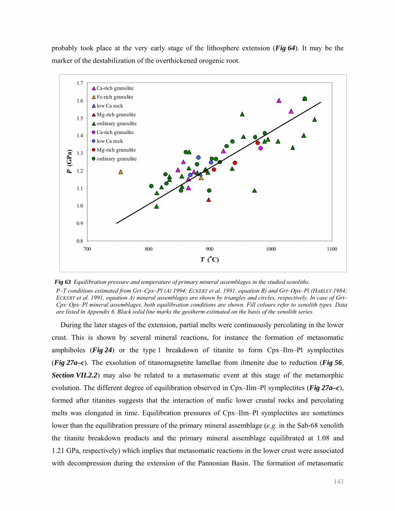
143
probably took place at the very early stage of the lithosphere extension (Fig 64). It may be the
marker of the destabilization of the overthickened orogenic root.
Fig 63 Equilibration pressure and temperature of primary mineral assemblages in the studied xenoliths. P–T conditions estimated from Grt–Cpx–Pl (AI 1994; ECKERT et al. 1991, equation B) and Grt–Opx–Pl (HARLEY 1984; ECKERT et al. 1991, equation A) mineral assemblages are shown by triangles and circles, respectively. In case of Grt–Cpx–Opx–Pl mineral assemblages, both equilibration conditions are shown. Fill colours refer to xenolith types. Data are listed in Appendix 6. Black solid line marks the geotherm estimated on the basis of the xenolith series.
During the later stages of the extension, partial melts were continuously percolating in the lower
crust. This is shown by several mineral reactions, for instance the formation of metasomatic
amphiboles (Fig 24) or the type 1 breakdown of titanite to form Cpx–Ilm–Pl symplectites
(Fig 27a–c). The exsolution of titanomagnetite lamellae from ilmenite due to reduction (Fig 56,
Section VII.2.2) may also be related to a metasomatic event at this stage of the metamorphic
evolution. The different degree of equilibration observed in Cpx–Ilm–Pl symplectites (Fig 27a–c),
formed after titanites suggests that the interaction of mafic lower crustal rocks and percolating
melts was elongated in time. Equilibration pressures of Cpx–Ilm–Pl symplectites are sometimes
lower than the equilibration pressure of the primary mineral assemblage (e.g. in the Sab-68 xenolith
the titanite breakdown products and the primary mineral assemblage equilibrated at 1.08 and
1.21 GPa, respectively) which implies that metasomatic reactions in the lower crust were associated
with decompression during the extension of the Pannonian Basin. The formation of metasomatic
0.8
0.9
1.0
1.1
1.2
1.3
1.4
1.5
1.6
1.7
700 800 900 1000 1100
T (oC)
P (G
Pa)
Ca-rich granuliteFe-rich granulitelow Ca rockMg-rich granuliteordinary granuliteCa-rich granulitelow Ca rockMg-rich granuliteordinary granulite
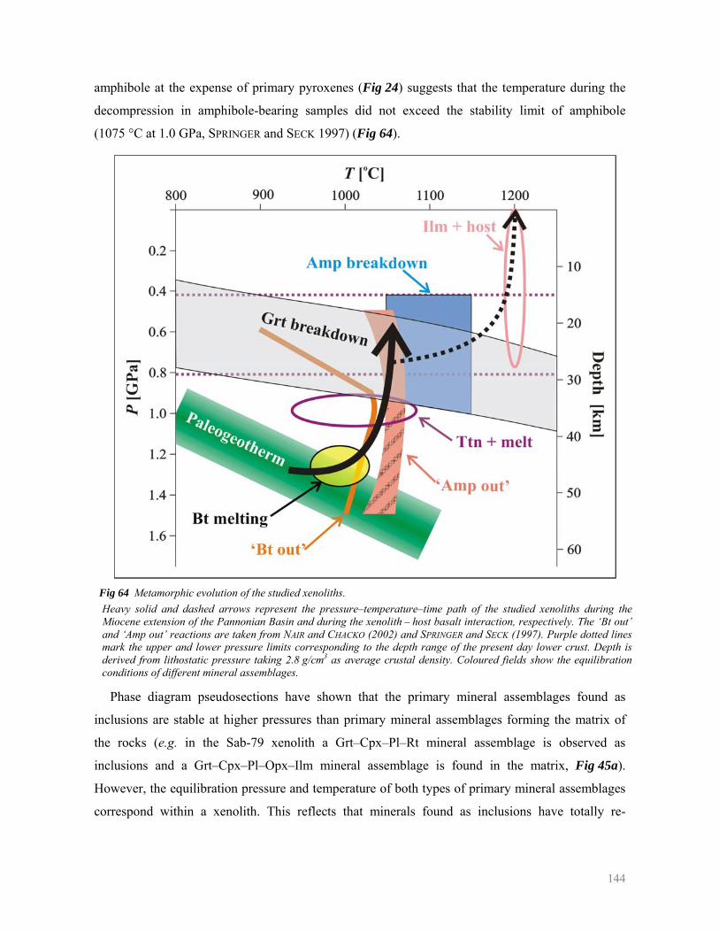
144
amphibole at the expense of primary pyroxenes (Fig 24) suggests that the temperature during the
decompression in amphibole-bearing samples did not exceed the stability limit of amphibole
(1075 °C at 1.0 GPa, SPRINGER and SECK 1997) (Fig 64).
Fig 64 Metamorphic evolution of the studied xenoliths. Heavy solid and dashed arrows represent the pressure–temperature–time path of the studied xenoliths during the Miocene extension of the Pannonian Basin and during the xenolith – host basalt interaction, respectively. The ‘Bt out’ and ‘Amp out’ reactions are taken from NAIR and CHACKO (2002) and SPRINGER and SECK (1997). Purple dotted lines mark the upper and lower pressure limits corresponding to the depth range of the present day lower crust. Depth is derived from lithostatic pressure taking 2.8 g/cm3 as average crustal density. Coloured fields show the equilibration conditions of different mineral assemblages.
Phase diagram pseudosections have shown that the primary mineral assemblages found as
inclusions are stable at higher pressures than primary mineral assemblages forming the matrix of
the rocks (e.g. in the Sab-79 xenolith a Grt–Cpx–Pl–Rt mineral assemblage is observed as
inclusions and a Grt–Cpx–Pl–Opx–Ilm mineral assemblage is found in the matrix, Fig 45a).
However, the equilibration pressure and temperature of both types of primary mineral assemblages
correspond within a xenolith. This reflects that minerals found as inclusions have totally re-
145
equilibrated with the matrix-forming primary mineral assemblage due to pressure decrease at the
very early stage of the metamorphic evolution.
The most frequently occurring mineral reaction in the xenoliths, the breakdown of garnet was
also the result of decompression. Element distributions in fine-grained symplectites after garnet
(Fig 51a) and mass balance considerations (Section VI.3.1) have shown that the
Grt = Al-Opx + An + Spl reaction was isochemical. Based on the thermodynamic analysis of
symplectite microstructures formed in the reaction (Section VI.3), the garnet breakdown took place
due to decompression most probably very slowly close to the stability limit of garnet. This
corresponds to pressures of the present day, thinned lower crust. In samples, where the garnet
stability extends to even lower pressures (e.g. in Sab-59 xenolith the lower pressure limit of garnet
stability is 0.44 GPa at 920 °C), the pressure decrease is shown by the decrease in Ca concentration
at the garnet rim (Fig 29) instead of the formation of symplectites after garnet. Probably this
reaction is the last mineralogical change during the extension of the basin.
A series of later mineral reactions seem to be the result of xenolith – host basalt interaction. This
is reflected by significant temperature increase and intense chemical interaction. The lack of garnet
in the amphibole melting products (Fig 25) and the high temperatures of the phases formed in the
reaction (1030–1120 °C), implies that the melting of amphiboles is the result of intense heating
during the interaction with the host basalt. In addition, olivine occurring in the melting products
indicates that the infiltrating host melt was partly involved in the reaction. Type 2 biotite melting
(Fig 23c–d) is also interpreted as the result of increased temperature during xenolith – host basalt
interaction. The crystallization of plagioclase overgrowth on primary plagioclase grains (Fig 22) is
the product of a chemical reaction with infiltrating melts. Although the thermodynamic analysis of
scapolite breakdown is not possible, the formation of spongy plagioclase coronas (Fig 26) after
scapolite may be the result of rapid decompression during the volcanic uplift of the xenoliths.
Several processes connected to xenolith – host basalt interaction obliterate fine-grained
symplectites formed in isochemical garnet breakdown. The recrystallization of type 1 symplectite
(Fig 21) is observed nearly in all samples where the symplectite is in connection with melt films on
grain boundaries. The enrichment of Na and Ti in the recrystallized reaction products
(Section VI.1.2) indicates that the host basalt was involved in the reaction. The formation of
olivine-bearing type 2 symplectite is also interpreted as a chemical reaction between fine-grained
type 1 symplectites and infiltrating host basalt. The melting of type 1 symplectite in amphibole-
bearing samples (Fig 51d) may have been induced by increased temperature and water activity.
The strongest evidence for intense interaction of the xenoliths with the host basalt is the
formation of complex chemical zoning patterns in Ilm–Tmt intergrowths (Fig 58). Oxide
146
thermometry have shown that right at the interface between primary ilmenites and titanomagnetite
overgrowth from the host basalt local chemical equilibrium at 1200 °C is achieved. At the same
time, the composition of titanomagnetite lamellae exsolved from ilmenite during the extension is
totally obliterated by Fe–Ti exchange with the titanomagnetite corona. By the diffusion modelling
of chemical zoning patterns in these titanomagnetite lamellae, the duration of this chemical
interaction was estimated to be 9–20 hours (Fig 62). This implies that the composition of lower
crustal mineral assemblages, even in xenoliths where silicates are not effected by the xenolith –
host basalt interaction, may be significantly modified during the rapid uplift of the xenoliths to the
surface.
147
SUMMARY OF THE MAIN RESULTS
Lower crustal mafic granulite xenoliths hosted in post-extensional alkali basalts of the BBHVF were investigated in this study by means of detailed petrography, mineral chemistry, thermodynamic modelling and geothermobarometric analysis of mineral assemblages observed in the samples combined with high resolution electron beam microanalytical studies, thermodynamic and diffusion modelling of reaction microstructures. The metamorphic evolution of the lower crust beneath the studied area was constructed and correlated with three main tectonometamorphic events: Alpine orogeny (1), Miocene basin extension (2) and interaction of the xenoliths with the host magma (3).
(1) Primary mineral assemblages in the studied xenoliths preserved a 15 °C/km paleogeotherm from the lower crustal lithospheric column of the overthickened Alpine orogenic root between 35 and 57 km depths and 800–1100 °C temperature. This lower crustal material show small scale chemical heterogeneities characteristic for the lower crust reworked during Andes-type subduction.
(2) At the early stage of the basin extension biotite-bearing rocks were partially molten due to infiltration of CO2-rich fluids. Melts produced in partial melting were continuously percolating in the lower crust during the extension of the Pannonian Basin. They reacted with primary minerals to form metasomatic mineral assemblages at different pressures. The pressure decrease due to lithosphere thinning induced the isochemical breakdown of garnet.
(3) According to diffusion modelling of complex chemical zoning patterns in titanomagnetites, the xenolith – host basalt interaction was extremely short (9–20 hours). Within this time interval the composition of titanomagnetites was completely reset, fine-grained reaction products formed in the lower crust were significantly modified, melting of hydrous phases was induced and primary phases reacted with the host basalt resulting in significant change in bulk rock chemistry.
Besides determining the metamorphic evolution of the lower crust, four main results were achieved. 1) I organized 5083 quantitative point analyses from 1135 phases in 67 thin sections together with images, line analyses and element distribution maps in a newly developed MS Access database, called GRANULITE, which served as a basis of the Ph.D. work and as the ultimate tool for data processing in this study because its data structure and built-in calculations are optimized for processing large amounts of data effectively during mineral chemical and geothermobarometric analyses. 2) The GRANULITE database provided model for the web-based Deep Lithosphere DataBase. 3) I tested several geothermobarometric methods and I selected the ones best applicable for these rocks. 4) TEM investigations combined with thermodynamic modelling of symplectitic microstructures after garnet established the basis of a new geospeedometric method.
148
MAGYAR NYELVŰ ÖSSZEFOGLALÓ
Doktori munkám során a Bakony–Balaton-felvidék vulkáni területről származó, poszt-extenziós alkáli bazalatokban és bazalttufákban előforduló alsó kéreg eredetű mafikus xenolitokat tanulmányoztam. A xenolitok kőzetalkotó, elsődleges ásványtársulásainak részletes petrográfiai és ásványkémiai vizsgálatát, termodinamikai modellezését és geotermobarometriai elemzését kiegészítettem a kőzetben megjelenő reakciószövetek nagyfelbontású elektronsugaras analitikai módszerekkel történő mikro- és nanoskálájú vizsgálatával, valamint termodinamikai és diffúziós modellezésével abból a célból, hogy a vizsgált terület alatti alsó kéreg fejlődésére vonatkozó adatokat pontosítsam. Vizsgálataim alapján az alsó kéreg tektonometamorf fejlődéstörténete három szakaszra osztható: alpi orogenezis (1), a Pannon medence miocén extenziója (2), valamint a xenolitok és a befogadó bazalt közötti kölcsönhatás (3).
(1) A kőzetben megjelenő elsődleges ásványtársulások megőrizték az alpi orogén gyökér 35 és 57 km közötti mélységben található 15 °C/km meredekségű paleogeotermáját, ahol a mélység növekedésével a hőmérséklet 800 °C-ról 1100 °C-ra nőtt. Az alsó kéreg anyaga ebben az időszakban erőteljes, centiméter skálájú kémiai heterogenitást mutatott, ami jó összhangban van az Andok-típusú szubdukció során átforgatott alsó kéreg reológiai felépítésével.
(2) A Pannon-medence extenziójának bevezető szakaszában CO2-gazdag fluidumok beáramlásának hatására a biotit-tartalmú kőzetek parciális olvadásnak indultak. Az így képződött olvadékok az extenzió során folyamatos nyomáscsökkenés mellett állandó jelleggel perkoláltak az alsó kéregben, és számos esetben reagáltak az elsődleges ásványokkal új, metaszomatikus ásványegyütteseket létrehozva. A nagymértékű nyomáscsökkenés az extenzió befejező szakaszában izokémikus gránát utáni szimplektitek képződéséhez vezetett.
(3) A Fe–Ti-oxidokban megfigyelhető komplex kémiai zónásság diffúziós modellezésével kimutattam, hogy a xenolit – befogadó bazalt kölcsönhatás átlagosan 9–20 órát vett igénybe. Ezen rendkívül rövid időtartamon belül az alsó kéregben képződött titanomagnetitek összetétele teljesen, míg a finomszemcsés reakciótermékek összetétele és mikroszerkezete jelentősen megváltozott, a beszivárgó bazalt reagált több elsődleges ásvánnyal, valamint az OH-tartalmú fázisok is olvadásnak idultak a nagy hőhatás következtében, ezáltal a teljes kőzet összetétele jelentősen módosult.
A vizsgált terület alatti alsó kéreg metamorf fejlődéstörténetén túl doktori munkám 4 fontos új eredményt hozott. 1) Megalkottam a GRANULITE nevű, a dolgozat alapjául szolgáló 67 csiszolat 1135 fázisából készített 5083 kvantitatív pontelemzést magába foglaló egységes adatbázist MS Access-ben. 2) Ezen adatbázis mintáján létrehoztuk a web-alapú egységes mélylitoszféra adatbázist (DLDB). 3) Összehasonlítottam és teszteltem számos geotermobarometriai módszert és megalkottam a vizsgált kőzetre optimális geotermobarometriai analízis metódusát. 4) A gránát után képződött finomszemcsés szimplektitek TEM-vizsgálata és termodinamikai modellezése alapot teremtett egy szimplektit mikroszerkezet-fejlődést leíró metamorf reakciósebességi vizsgálat későbbi kidolgozásához.
i
REFERENCES
A ABART R, PETRISHCHEVA E, FISCHER FD, SVOBODA J (2009) Thermodynamic model for diffusion
controlled reaction rim growth in a binary system: Application to the forsterite-enstatite-quartz system: Amer J Sci 309: 114–131
AGGARWAL A, TOPFER J, TSAI TL, DIECKMANN R (1997) Point defects and transport in binary and ternary, non-stoichiometric oxides. Solid State Ionics 101–103: 321–331
AGGARWAL S, DIECKMANN R (2002) Point defects and cation tracer diffusion in (TixFe1−x)3−δO4. II. Cation tracer diffusion. Phys Chem Miner 29: 707–718
AI Y (1994) A revision of the garnet-clinopyroxene Fe2+-Mg exchange geothermometer. Contrib Mineral Petrol 115: 467–473
ALTHERR R, KALT A (1996) Metamorphic evolution of ultrahigh-pressure garnet peridotite from the Variscan Vosges Mts. (France). Chem Geol 134: 27–47
ANDERSEN DJ, LINDSLEY DH (1988) Internally consistent solution models for Fe–Mg–Mn–Ti oxides: Fe–Ti oxides. Am Mineral 73: 714–726
ARAGON R, MCCALLISTER RH, HARRISON HR (1984) Cation diffusion in titanomagnetites. Contrib Mineral Petrol 85: 174–185
ARCULUS RJ, SMITH D (1979) Ecologite, pyroxenite, and amphibolite inclusions in kimberlites and other volcanics in Sullivan Buttes latite, Chino Valley, Yavapai county, Arizona. In: BOYD FR, MEYER HOA (Eds) The Mantle Sample. Am Geophys Union Mon 309–317
ARMSTRONG JT (1991) Quantitative elemental analysis of individual microparticles with electron beam instruments. In: HEINRICH KJF, NEWBURY DE (Eds) Electron Probe Quantification. Plenum Press, New York, 261-315
ARMSTRONG JT (1995) CITZAF: a package of correction programs for the quantitative electron microbeam X-ray analysis of thick polished materials, thin films, and particles. Microbeam Anal 4: 177-200
ASHWORTH JR, CHAMBERS AD (2000) Symplectitic reaction in olivine and the controls on intergrowth spacing in symplectites. J Petrol 41(2): 285–304
ASHWORTH JR, SHEPLEV VS (1997) Diffusion modeling of metamorphic layered coronas with stability criterion and consideration of affinity. Geochimica et Cosmochimica Acta 61: 3671–3689
B BADA G, HORVÁTH F, DÖVÉNYI P, SZAFIÁN P (2007) Prersent-day stress field and tectonic
inversionin the Pannonian basin. Global and Planet Change 58: 165–180 BADA G, HORVÁTH F, GERNER, P, FEJES I (1999) Review of the present-day geodynamics of the
Pannonian basin: progress and problems. Journal of Geodynamics 27(4-5): 501–527 BADENSZKI E (2004) Szentbékkállai bázisos xenolitok petrológiai vizsgálata. Thesis for the
National Scientific Conference of Students, Eötvös University, Budapest BADENSZKI E (2006) A szentbékkállai és szigligeti bázisos granulit xenolitok kőzettani vizsgálata.
MSc Thesis, Eötvös University, Budapest BALI E, FALUS G, SZABÓ CS, PEATE DW, HIDAS K, TÖRÖK K, NTAFLOS T (2007) Remnants of
boninitic melts in the upper mantle beneath the central Pannonian Basin? Mineralogy and Petrology 90: 51–72
ii
BALI E, SZABÓ CS, VASELLI O, TÖRÖK K (2002) Significance of silicate melt pockets in upper mantle xenoliths from the Bakony–Balaton Highland Volcanic Field, Western Hungary. Lithos 61: 79-102
BALI E, ZAJACZ Z, KOVÁCS I, SZABÓ CS, HALTER W, VASELLI O, TÖRÖK K, BODNAR RJ (2008b) A quartz-bearing orthopyroxene-rich websterite xenolith from the Pannonian Basin, Western Hungary: Evidence for release of quartz-saturated melt from a subducted slab. Journal of Petrology 49: 421–439
BALI E, ZANETTI A, SZABÓ CS, PEATE D, WAIGH TE (2008a) Evolution of the subcontinental lithospheric mantle beneath the Central Pannonian Basin: trace element evidence from silicate melt pockets in mantle xenoliths from the Bakony-Balaton Highland Volcanic Field, (western Hungary). Contributions to Mineralogy and Petrology 155: 165–179
BALLA Z (1987) Tertiary paleomagnetic data for the Carpatho Pannonian region in the light of Miocene rotation kinematics. Tectonophysics 139: 67–98
BALLA Z (1988) Clockwise paleomagnetic rotations in the Alps in the light of the structural pattern of the Transdanubian Range (Hungary). Tectonophysics 145: 277-292
BALOGH K, ÁRVA-SÓS E, PÉCSKAY Z, RAVASZ-BARANYAI L (1986) K/Ar dating of Post-Sarmatian alkali basaltic rocks in Hungary. Acta Miner-Petr 28: 75-84
BALOGH K, EBNER F, RAVASZ CS, HERRMANN P, LOBITZER H, SOLTI G (1994) K/Ar Alter tertiare Vulkanite der südstlichen Steiermark und südlichen Burgenlands. In: LOBITZER H, CSÁSZÁR G DAURER A (Eds) Jubilaumschrift 20 Jahre geologische Zusammenarbeit Österreich-Ungarn. Geologische Bundesanstalt 2: 55–72
BÉRCZI I (1988) Preliminary sedimentological investigation of a Neogene depression. In: ROYDEN LH, HORVÁTH F (1988) 107–116
BÉRCZI I, HÁMOR G, JÁMBOR Á, SZENTGYÖRGYI K (1988) Neogen sedimentation in Hungary. In: ROYDEN LH, HORVÁTH F (1998) 57–67.
BERKESI M, HIDAS K, SZABÓ CS (2007) Fossil geotherm estimation of spinel peridotites from Tihany (Bakony–Balaton Highland Volcanic Field) based on CO2 inclusions. Magyar Geofizika (in Hungarian with English abstract) 48: 31–37
BUDDINGTON AF, LINDSLEY DH (1964) Iron-titanium oxide minerals and synthetic equivalents. J Petrol 5: 310–357
C CAHN JW (1959) The kinetics of cellular segregation reactions. Acta Metall 7: 18–28 CARSWELL DA, MOILER C, O'BRIEN PJ (1989) Origin of sapphirine-plagioclase symplectites in
metabasites from Mitterbachgraber, Dunkelsteinerwald granulite complex, Lower Austria. Eur J Mineral 1: 455–466
CHANNELL JET, KOZUR HW (1997) How many oceans? Meliata, Vardar, and Pindos oceans in Mesozoic Alpine paleogeography. Geology 25: 183–186
COLTORTI M, BONADIMAN C, FACCINI B, NTAFLOS T, SIENA F (2007) Slab melt and intraplate metasomatism in Kapfenstein mantle xenoliths (Styrian Basin, Austria). Lithos 94: 66–89
CONNOLLY JAD (1990) Multivariable phase diagrams: an algorithm based on generalized thermodynamics. Am J Sci 290: 666–718
CREWE AV, WALL J, WELTER LM (1968) Electron Gun Using a Field Emission Source. The review of Scientific Instruments 39(4): 576–583
CSONTOS L (1995) Tertiary tectonic evolution of the Intra-Carpathian area: A review. Acta Vulcanologica 7: 1–13
iii
CSONTOS L, NAGYMAROSY A (1998) The Mid-Hungarian line: a zone of repeated tectonic inversions. Tectonophysics 297: 51–71
CSONTOS L, NAGYMAROSY A, HORVÁTH F, KOVÁCS M (1992) Tertiary evolution of the Intra-Carpatian area: a model. Tectonophysics 208: 221–241
CSONTOS L, VÖRÖS A (2004) Mesozoic plate tectonic reconstruction of the Carpathian region. Palaeogeography, Palaeoclimatology, Palaeoecology 210(1): 1–56
D DÉGI J (2004) Petrographic evidence of crustal thinning in Bakony–Balaton Highland Volcanic
Field (in Hungarian). MSc Thesis in Geology Department of Petrology and Geochemistry, Eötvös University, Budapest, pp 112
DÉGI J (2008) Geothermobarometry — A new database for the comparison of mineral chemistry and different geothermobarometric methods for metamorphic rocks. 33rd International Geological Congress (IGC), 6-14 August 2008, Oslo
DÉGI J, ABART R, TÖRÖK K, BALI E, WIRTH R, RHEDE D (in press) Symplectite formation during decompression induced garnet breakdown in lower crustal mafic granulite xenoliths: mechanisms and rates. Contrib Mineral Petrol DOI: 10.1007/s00410-009-0428-z
DÉGI J, ABART R, TÖRÖK K, RHEDE D, PETRISHCHEVA E (2009) Evidence for xenolith – host basalt interaction from chemical patterns in Fe–Ti-oxides from mafic granulite xenoliths of the Bakony–Balaton Volcanic field (W-Hungary). Mineral Petrol 95(3): 219–234
DÉGI J, TÖRÖK K (2003) Petrographic evidence of crustal thinning in Bakony–Balaton Highland Volcanic Field (in Hungarian). Magyar Geofizika 44(4): 125–133
DEMÉNY A, VENNEMAN TW, HEGNER E, NAGY G, MILTON JA, EMBEY-ISZTIN A, HOMONNAY Z, DOBOSI G (2004) Trace element and C–O–Sr–Nd isotope evidence for subduction-related carbonate–silicate melts in mantle xenoliths (Pannonian Basin, Hungary). Lithos 75(1/2): 89–113
DIECKMANN R (1998) Point defects and transport in non-stoichiometric oxides: solved and unsolved problems. J Phys Chem Solids 59: 507–525
DIECKMANN R, SCHMALZRIED H (1977) Defects and cation diffusion in magnetite (I). Ber Bunsenges Phys Chem 81: 344–347
DING L, ZHONG D (1999) Metamorphic characteristics and geotectonic implications of the high-pressure granulites from Namjagbarwa, eastern Tibet. Science in China (D) 42: 491–505
DOBOSI G, KEMPTON P, DOWNES H, EMBEY-ISZTIN A, THIRLWALL M, GREENWOOD P (2003) Lower crustal xenoliths from the Pannonian Basin, Hungary. Part 2: Sr-Nd-Pb-Hf and O isotope evidence for formation of continental lower crust by tectonic emplacement of oceanic crust. Contrib. Mineral. Petrol 144: 671–683
DOMBRÁDI E, TÍMÁR G, BADA G, CLOETINGH S, HORVÁTH F (2007) Fractal dimension estimations of drainage network in the Carpathian–Pannonian system. Global and Planetary Change 58: 197–213
DÖVÉNYI P (1994) Geofizikai vizsgálatok a Pannon-medence litoszférafejlődésének megértéséhez. PhD Thesis, ELTE, Budapest
DÖVÉNYI P, HORVÁTH F (1988) A review of temperature thermal conductivity and heat flow data from the Pannonian basin. In: ROYDEN LH, HORVÁTH F (1998) 195–233
DOWNES H, EMBEY-ISZTIN A, THIRLWALL MF (1992) Petrology and geochemistry of spinel peridotite xenoliths from the western Pannonian Basin (Hungary) evidence for an association between enrichments and texture in the upper mantle. Contrib. Mineral. Petrol 109: 340–354
iv
DOWNES H, SEGHEDI I, SZAKACS A, DOBOSI G, JAMES DE, VASELLI O, RIGBY IJ, INGRAM GA, REX D, PECSKAY Z (1995b) Petrology and geochemistry of late Tertiary/Quaternary mafic alkaline volcanism in Romania. Lithos 35: 65–81
DOWNES H, VASELLI O (1995) The lithospheric mantle beneath the Carpathian-Pannonian Region: review of trace elements and isotopic evidence of ultramafic xenoltihs. In: DOWNES H, VASELLI O (eds) Neogene and realted magmatism in the Carpatho-Pannonian Region. Acta Volc 7: 219–229
DOWNES H, VASELLI O, SEGEDHI I, INGRAM G, REX D, CARDOSSI N, PÉCSKAY Z, PINARELLI L (1995a) Geochemistry of late Cretaceous - early Tertiary magmatism in Poiana Rusca (Romania). Acta Vulcanologica 7: 209–217
DROOP GTR (1987) A general equation for estimating Fe3+ concentration in ferromagnesian silicates and oxides from microprobe analyses, using stoichiometric criteria, Mineral. Mag 51: 431–435
DUDECK A, FEDIUKOVA E (1974) Eclogites of the Bohemian Moldanubicum. Neues Jahrb Mineral Abh 121: 127–159
E ECKERT JO, NEWTON RC, KLEPPA OJ (1991) The ΔH of reaction and recalibration of garnet–
pyroxene-plagioclase-quartz geobarometers in the CMAS system by solution calorimetry. Amer Mineral 76: 148–160
ELLIS DJ, GREEN D (1979) An experimental study of the effect of Ca upon garnet-clinopyroxene Fe-Mg exchange equilibria. Contrib. Mineral. Petrol 71: 13–22
EMBEY-ISZTIN A (1978) On the petrology of spinel lherzolite nodules in basaltic rocks in Hungary and Auvergne, France. Ann Hist Nat Mus Nat Hung 70: 27–44
EMBEY-ISZTIN A, DOBOSI G (1995) Source mantle characteristics beneath the Carpathian-Pannonian Region: a review of trace element and isotopic evidence from Pliocene to Quaternary alkali basalts. Acta Vulcanol 7: 155–166
EMBEY-ISZTIN A, DOBOSI G, ALTHERR R, MEYER HP (2001a) Thermal evolution of the lithosphere beneath the western Pannonian Basin: evidence from deep-seated xenoliths. Tectonophysics 331: 285–306
EMBEY-ISZTIN A, DOBOSI G, DOWNES H (2001b) Geochemical characterization of the Pannonian Basin mantle lithosphere and asthenosphere: an overview. Acta Geol Hung 44: 259–280
EMBEY-ISZTIN A, DOBOSI G, NOSKE-FAZEKAS G, ÁRVA-SÓS E (1989) Petrology of a new basalt occurence in Hungary. Mineral Petrol 40: 183–196
EMBEY-ISZTIN A, DOWNES H, JAMES DE, UPTON BGJ, DOBOSI G, INGRAM G, HARMON RS, SCHARBERT HG (1993) The petrogenesis of Pliocene alkaline volcanic rocks from the Pannonian Basin, Eastern Central Europe. Journal of Petrology 34: 317–343
EMBEY-ISZTIN A, DOWNES H, KEMPTON P, DOBOSI G, THIRLWALL M (2003) Lower crustal xenoliths from the Pannonian Basin, Hungary. Part 1: mineral chemistry, thermobarometry and petrology. Contrib Mineral Petrol 144: 652–670
EMBEY-ISZTIN A, SHARBERT HG, DIETRICH H, POULTIDIS H (1990) Mafic granulites and clinopyroxenite xenoliths from the Transdanubian Volcanic Region (Hungary): implications for the deep structure of the Pannonian Basin. Mineral Mag 54: 463-483
v
F FACCENDA M, GERYA T, CHAKRABORTY S (2008) Styles of post-subduction collisional orogeny:
Influence of convergence velocity, crustal rheology and radiogenic heat production. Lithos 103(1–2): 257–287
FALUS GY, DRURY MR, VAN ROERMUND HLM, SZABÓ CS (2004) Magmatism related localized deformation in the mantle: a case study. Contributions to Mineralogy and Petrology 146: 493–505
FALUS GY, SZABÓ CS, KOVÁCS I, ZAJACZ Z, HALTER W (2007) Symplectite in spinel lherzolite xenoliths from the Little Hungarian Plain, Western Hungary: a key for understanding basin evolution. Lithos 94: 230–247
FALUS GY, SZABÓ CS, VASELLI O (2000) Mantle upwelling within the Pannonian Basin: evidence from xenolith lithology and mineral chemistry. Terra Nova 12: 295-302
FALUS GY, TOMMASI A, INGRIN J, SZABÓ CS (2008) Deformation and seismic anisotropy of the lithospheric mantle in the southeastern Carpathians inferred from the study of mantle xenolith. Earth and Planetary Science Letters 272: 50–64
FIALA J (1966) The distribution of elements in mineral phases of some garnet lherzolites from the Bohemian massif. Krystalinikum 4: 31–53
FODOR L, BADA G, CSILLAG G, HORVÁTH E, RUSZKICZAY-RÜDIGER ZS, PALOTÁS K, SÍKHEGYI F, TIMÁR G, CLOETINGH S, HORVÁTH F (2005) An outline of neotectonic structures and morphotectonics of the western and central Pannonian basin. Tectonophysics 410: 15–41
FODOR L, CSONTOS L, BADA G, GYŐRFI I, BENKOVICS L (1999) Tertiary tectonic evolution of the Pannonian basin system and neighbouring orogens, a new synthesis of paleostress data. In: DURAND B, JOLIVET L, HORVÁTH F, SÉRANNE M (Eds) The Mediterranean Basins: Tertiary extension within the Alpine Orogen. Geological Society, London, Special Publications 156: 295–334
FOLEY SF, ANDRONIKOV AV, JACOB DE, MELZER S (2006) Evidence from Antarctic mantle peridotite xenoliths for changes in mineralogy, geochemistry and geothermal gradients beneath a developing rift. Geochimica et Cosmochimica Acta 70: 3096–3120
FREER R (1980) Self-diffusion and impurity diffusion in oxides. J Mater Sci 15: 803–824 FREER R, HAUPTMAN Z (1978) An experimental study of magnetite–titanomagnetite interdiffusion.
Phys Earth Planet Inter 16: 223–231
G GANGULY J, CHENG W, CHAKRABORTY S (1998) Cation diffusion in aluminosilicate garnets:
experimental determination in pyrope-almandine diffusion couples. Contrib Mineral Petrol 131: 171–180
GÉCZY B (1973) The origin of the Jurassic faunal provinces and the Mediterranean plate tectonics. Ann Univ Sci Bp R Eötvös nom Sect Geol 16: 99–114
GHIORSO MS, EVANS BW (2008) Thermodynamics of rhombohedral oxide solid solutions and a revision of the Fe-Ti two-oxide geothermometer and oxygen-barometer. Am J Sci 308: in press
GHIORSO MS, SACK RO (1991) Fe- Ti oxide geothermometry: thermodynamic formulation and the estimation of intensive variables in silicic magmas. Contrib Mineral Petrol 108: 485–510
GMÉLING K, NÉMET K, MARTIN U, EBY N, VARGA ZS (2007) Boron concentrations of volcanic fields in different geotectonic settings. Journal of Volcanology and Geothermal Research 159: 70–84
vi
GODARD G, MARTIN S (2000) Petrogenesis of kelyphites in garnet peridotites: a case study from the Ulten zone, Italian Alps. J Geodyn 30: 117–145
GREEN DH, RINGWOOD AE (1967) An experimental investigation of the gabbro to eclogite transformation and its petrological applications. Geochimica et Cosmochimica Acta 31: 767–833
GRENERCZY GY (2002) Tectonic processes in the Eurasian-African plate boundary zone revealed by space geology. In: STEIN S, FREYMUELLER JT (Eds.), Plate boundary zones. AGU Monograph, Geodyn Ser 30: 67-86
GRENERCZY GY, KENYERES A, FEJES I (2000) Present crustal movement and strain distribution in Central Europe inferred from GPS measurements. J Geophys Res 105: 21835-21856
GRENERCZY GY, SELLA GF, STEIN S, KENYERES A (2005) Tectonic implications of the GPS velocity field in the northern Adriatic region. Geophysical Research Letters 32: L16311
GRIFFIN WL, HEIER KS (1973) Petrological implication of some corona structures. Lithos 6: 315–335
H HAGGERTY SE (1991) Oxide textures — a mini-atlas. In: LINDSLEY DH (Ed) Oxide minerals:
petrologic and magnetite significance. Rev Mineral 25: 129–137 HAMMOND PL, TOMPKINS LA, HAGGERTY SE, TAYLOR SE, SPENCER KJ, LINDSLEY DH (1982)
Revised data for coexisting magnetite and ilmenite near 1000°C, NNO and FMQ buffers. GSA Meeting. Abstr Progr 14: 506
HARANGI R, HARANGI SZ (1995) Volcanological study of the Neogene basaltic volcano of Sághegy (Little Hungarian Plain Volcanic, Western Hungary). Acta Vulcanologica 7: 173–189
HARANGI SZ (2001) Neogene to Quartenary volcanism of the Carpatian-Pannonian Region – A review: Acta Geologica Hungarica 44: 223–258
HARANGI SZ, WILSON M, TONARINI S (1995) Petrogenesis of Neogene potassic volcanic rocks in the Pannonian Basin. Acta Vulcanol 7: 125–134
HARLEY SL (1984) The solubility of alumina in orthopyroxene coexisting with garnet in FeO-MgO-Al2O3-SiO2 and CaO-FeO-MgO-Al2O3-SiO2. J Petrol 25: 665–696.
HARLEY SL (1989) The origins of granulites: a metamorphic prospective. Geological Magazine 126: 215–247
HARLOV DE (2000) Titaniferous magnetite±ilmenite thermometry and titaniferous magnetite± ilmenite± orthopyroxene± quartz oxygen barometry in granulite facies gneisses, Bamble Sector, SE Norway: implications for the role of high-grade CO2-rich fluids during granulite genesis. Contrib Mineral Petrol 1139: 180–197
HARLOV DE, HANSEN EC (2005) Oxide and sulphide isograds along a Late Archean, deep-crustal profile in Tamil Nadu, south India. J Metamorph Geol 23: 241–259
HIDAS K, FALUS G, SZABÓ CS, SZABÓ PJ, KOVÁCS I, FÖLDES T (2007) Geodynamic implications of flattened tabular equigranular textured peridotites from the Bakony-Balaton Highland Volcanic Field (Western Hungary). Journal of Geodynamics 43: 483–503
HOLLAND T, POWELL R (1996). Thermodynamics of order-disorder in minerals; II, Symmetric formalism applied to solid solutions. American Mineralogist 81: 1425–1437
HOLLAND TJB, POWELL R (1998) An internally consistent thermodynamic data set for phases of petrological interest. J Metamorph Geol 16: 309–343
HORVÁTH F (1993) Towards a mechanical model for the formation of the Pannonian basin. Tectonophysics 226: 333–357
vii
HORVÁTH F (1995) Phases of compression during the evolution of the Pannonian basin and its bearing on hydrocarbon exploration. Mar Petr Geol 12: 837–844
HORVÁTH F (2007) A Pannon-medence geodinamikája — Eszmetörténeti tanulmány és geofizikai szintézis. Doctoral Thesis, ELTE, Budapest, pp. 238
HORVÁTH F, BADA D, SZAFIÁN P, TARI G, ÁDÁM A, CLOETINGH, S (2005) Formation and deformation of the Pannonian basin: Costraints from observational data, In: GEE D, STEPHENSON R (Eds.) European Lithosphere Dynamics, EUROPROBE, Geol. Soc. London Memoirs, 32: 191–206
HORVÁTH F, CLOETINGH S (1996): Stress-induced late stage subsidence anomalies in the Pannonian basin. Tectonophysics 266: 287–300
HORVÁTH F, POGÁCSÁS GY (1988) Contribution of seismic reflection data chronostratigraphy of the Pannonian basin. In: ROYDEN LH, HORVÁTH F (1998) 69–77.
HUISMANS RS, PODLADCHIKOV YY, CLOETINGH S (2001) Dynamic modeling of the transition from passive to active rifting, application to the Pannonian basin. Tectonics 20: 1021–1039
J JARSOSEWICH E, NELEN JA, NORBERG JA (1980) Reference samples for electron microprobe
analysis. Geostand Newsl 4: 43–47 DE JONG AF, COENE W, VAN DYCK D (1989) Image processing of HRTEM images with non-
periodic features. Ultramicroscopy 37: 53–66
K KEANKEO W, TAYLOR WR, FITZGERALD JD (2000) Clinoferrosilite-bearing kelyphite: a breakdown
product of xenolithic garnet, Delegate breccia pipes, New South Wales, Australia. Mineral Mag 64(3): 469–479
KELLER LM, WIRTH R, RHEDE D, KUNZE K, ABART R (2008) Asymmetrically zoned reaction rims: assessment of grain boundary diffusivities and growth rates related to natural diffusion-controlled mineral reactions. J Metamorph Geol 26: 99–120
KEMPTON P, DOWNES H, EMBEY-ISZTIN A (1997) Mafic granulite xenoliths in Neogene alkali basalts from the Western Pannonian Basin: insights into the lower crust of a collapsed orogen. J Petrol 38: 941–970
KODOLÁNYI J (2004) Kapolcsi bázisos granulit xenolitok petrológiai vizsgálata. Thesis for the National Scientific Conference of Students, Eötvös University, Budapest
KODOLÁNYI J (2005) Redukció és hűlés nyomai a bondoró-hegyi alsó kéreg eredetű kőzetzárványokban. MSc Thesis, Eötvös University, Budapest
KONEČNÝ V, LEXA J, BALOGH K, KONECNY P (1995) Alkali basalt volcanism in Shouthern Slovakia: volcanic forms and time evolution. Acta Vulcanologica. 7: 167–173
KÓTHAY K, SZABÓ CS, TÖRÖK K, SHARYGIN V (2005) A droplet of the magma: Silicate melt inclusions in olivine phenocrysts from alkali basalt of Hegyestű. Földtani Közl 135: 31–55
KOVAĆ M, NAGYMAROSY A, OSZCZYPKO N, CSONTOS L, SLACZKA A, MARUNTEANU M, MATENKO L, MÁRTON E (1998) Palinspastic reconstruction of the Carpathian– Pannonian region during the Miocene. In: RAKUŠ M, (Ed) Geodynamic Development of the Western Carpathians: Bratislava. Geologický ústav Dionýza Štúra 198–217
KOVÁCS I, CSONTOS L, SZABÓ CS, BALI E, FALUS GY, BENEDEK K, ZAJACZ Z (2007) Paleogene–early Miocene igneous rocks and geodynamics of the Alpine-Carpathian-Pannonian-Dinaric region: An integrated approach. Geological Society of America Special Paper 418: 93–111
viii
KOVÁCS I, SZABÓ CS (2005) Petrology and geochemistry of granulite xenoliths beneath the Nógrád-GömörVolcanic Field, Carpathian-Pannonian Region (N-Hungary/S-Slovakia). Mineralogy and Petrology 85: 269–290
KOVÁCS I, SZABÓ CS (2008) Middle Miocene volcanism in the vicinity of the Middle Hungarian zone: evidence for an inherited enriched mantle source - A review: Journal of Geodynamics 45: 1-17
KOVÁCS I, ZAJACZ Z, SZABÓ CS (2004) Type-II xenoliths and related metasomatism from the Nógrád-Gömör Volcanic Field, Carpathian-Pannonian Region (northern Hungary – southern Slovakia). Tectonophysics 393: 139–161
KRETZ R (1983) Symbols for rock-forming minerals. Amer Mineral 68: 277-279 KROGH EJ (1988) The garnet-clinopyroxene Fe-Mg geothermometer — a reinterpretation of
existing experimental data. Contrib. Mineral. Petrol 99: 44–48 KURAT G, EMBEY-ISZTIN A, KARCHER A, SCHARBERT H (1991): The upper mantle beneath
Kapfenstein and the Transdanubian Volcanic Region, E-Austria and W-Hungary: A comparison. Mineral Petrol 44: 21–38
L LATTARD D (1995) Experimental evidence for the exsolution of ilmenite from titaniferous spinel.
Am Mineral 80: 968–981 LATTARD D, SAUERZAPF U, KÄSEMANN M (2005) New calibration data for the Fe–Ti oxide thermo-
oxybarometers from experiments in the Fe–Ti–O system at 1 bar, 1,000–1,300°C and a large range of oxygen fugacities. Contrib Mineral Petrol 149: 735–754
LEAKE BE (1978) Nomenclature of amphiboles. Am Mineral 63: 1023–1052 LENKEY L (1999) Geothermics of the Pannonian basin and its bearing on the tectonics of basin
evolution. PhD thesis, Vrije Univ., Amsterdam, pp. 215 LINDSLEY DH (1962) Investigations in the system FeO–Fe2O3–TiO2. Carnegie Inst Wash Yearb 61:
100–106 LINDSLEY DH (1963) Fe–Ti oxides in rocks as thermometers and oxygen barometers. Carnegie Inst
Wash Yearb 62: 60–66 LINDSLEY DH (1991) Experimental studies of oxide minerals. In: LINDSLEY DH (Ed) Oxide
minerals: petrologic and magnetic significance. Rev Mineral 25: 69–100 LIPPITSCH R, KISSLING E, ANSORGE J, (2003) Upper mantle structure beneath the Alpine orogen
from high-resolution teleseismic tomography. J Geophys Res 108(B8): 2376 LIU Y, ZHONG D (1997) Petrology of high-pressure granulites from the eastern Himalayan syntaxis.
Journal of Metamorphic Geology 15: 451–466
M MÁRTON E, DROBNE K, COSOVIC V, MORO A (2003) Palaeomagnetic evidence for Tertiary
counterclockwise rotation of Adria. Tectonophysics 377: 143–156 MÁRTON E, MAURITSCH HJ (1990) Structural applications and discussion of a paleomagnetic post-
Paleozoic database for the Central Mediterranean. Phys Earth Planet Int 62: 46–59 MASSONE HJ, WILMER AP (2008) Phase relations and dehydration behaviour of psammopelite and
mid-ocean ridge basalt at very-low-grade to low-grade metamorphic conditions. Eur J Mineral 20(5): 867–879
MCCARTHY TC, PATINO-DOUCE AE (1998) Empirical calibration of the silica-Ca-tschermak’s-anorthite (SCAn) geobarometer. J Metamorphic Geol 16: 675–686
ix
MCKENZIE D (1978) Some remarks on the development of sedimentary basins. Earth and Planet Sci Lett 40: 25–32
MESSIGA B, BETTINI E (1990) Reactions behaviour during kelyphite and a symplectite formation: a case study of mafic granulites and eclogites from the Bohemian Massif. Eur J Mineral 2: 125–44
MEULENKAMP JE, KOVAC M, CICHA I (1996) On late Oligocene to Pliocene depocentre migrations and the evolution of the Carpathian-Pannonian system. Tectonophysics 266: 301–317
MUKHOPADHYAY B (1991) Garnet breakdown in some deep seated garnetiferous xenoliths from the central Sierra Nevada: Petrologic and tectonic implications. Lithos 27: 59–78
N NAIR R, CHACKO T (2002) Fluid-absent melting of high-grade semipelites: P-T constraints on
orthopyroxene formation and implications for granulite genesis. J Petrol 43: 2121–2142 NAKANO N, OSANAI Y, THI MINH N, MIYAMOTO T, HAYASAKA Y, OWADA M (2008) Discovery of
high-pressure granulite-facies metamorphism in northern Vietnam: Constraints on the Permo-Triassic Indochinese continental collision tectonics. C R Geoscience 340: 127–138
NÉDLI ZS, M. TÓTH T (2007) Origin and geodynamic significance of Upper Cretaceous lamprophyres from the Villany Mts (S Hungary). Min Pet 90: 73–107
NEMCOK M, POSPISIL L, LEXA J, DONELICK RA (1998) Tertiary subduction and slab break-off model of the Carpathian-Pannonian region. Tectonophysics 295: 307–340
NÉMETH K, MARTIN U (1999a) Late hydrovolcanic field in the Pannonian basin: general characteristics of the Bakony-Balaton Highland Volcanic Field, Hungary. Acta Vulcanologica 11: 271-282
NÉMETH K, MARTIN U (1999b) Late Miocene paleo-geomorphology of the Bakony-Balaton Highland Volcanic Field (Hungary) using physical volcanology data. Z Geomorph N F 43: 417-438
NÉMETH B, BADENSZKI E, KOLLER F, TÖRÖK K, MOGASSIE A, SZABÓ CS (2009) Mid-crustal xenoliths from Beistein, Austria. EGU General Assembly. April 19-24, 2009, Vienna, Geophysical Research Abstracts 11(EGU2009): 5618
NEWTON RC, PERKINS D (1982) Thermodynamic calibration of geobarometers based on the assemblages garnet-plagioclase-orthopyroxene (clinopyroxene)-quartz: Am. Mineral 67(3/4): 203–222
O O’BRIEN PJ (2008) Challenges in high-pressure granulite metamorphism in the era of
pseudosections: reaction textures, compositional zoning and tectonic interpretation with examples from the Bohemian Massif. J Metamorphic Geol 26: 235–251
O’BRIEN PJ, RÖTZLER J (2003) High-Pressure Granulites: Formation, Recovery of Peak Conditions, and Implications for Tectonics. Journal of Metamorphic Geology 21: 3–20
OBATA M (1994) Material transfer and local equilibria in a zoned kelyphite from a garnet pyroxenite, Ronda, Spain. J Petrol 35: 271–87
ONSAGER L (1931) Reciprocal relations in irreversible processes. I. Physical Review 37: 405–426
P PADOVANI ELR, CARTER JL (1976) Non equilibrium partial fusion due to decompression and
thermal effects in crustal xenoliths. In: H.G.J. Dick (ed) Magma Genesis. Oreg. Dept. Geol. Mineral Ind Bull 96: 43–57
x
PATTISON DRM (2003) Petrogenetic significance of orthopyroxene-free garnet+clinopyroxene + plagioclase-bearing metabasites with respect to the amphibolite and granulite facies. Journal of Metamorphic Geology 21: 21–31
PATTISON DRM, CHACKO T, FARQUHAR J, MCFARLAINE CRM (2003) Temperatures of granulite-facies metamorphism: Constraints from experimental phase equilibria and thermobarometry corrected for retrograde exchange. J Petrol 44: 867-900
PATTISON DRM, NEWTON, R. C (1989): Reversed experimental calibration of the garnet-clinopyroxene Fe-Mg exchange thermometer. Contrib. Mineral. Petrol 101: 87–103
PÉCSKAY Z, LEXA J, SZAKÁCS A, BALOGH K, SEGHEDI I, KONECNY V, KOVÁCS M, MÁRTON E, KALICIAK M, SZÉKY-FUX V, PÓKA T, GYARMATI P, EDELSTEIN O, ROSU E, ZEC B (1995) Space and time distribution of Neogene-Quaternary volcanism in the Carpatho-Pannonian Region. Acta Vulcanol 7: 15–28
PETERSON JW, CHACKO T, KUEHNER SM (1991) The effects of fluorine on the vapor-absent melting of phlogopite + quartz: Implications for deep-crustal processes. Am Mineral 76: 470–476
PETERSON JW, NEWTON RC (1990) Experimental biotite-quartz melting in the KMASH-CO2 system and the role of CO2 in the petrogenesis of granites and related rocks. Am Miner 75: 1029–1042
POSGAY K, ALBU I, MAYEROVA M, NAKLADALOVA Z, IBRMAJER I, BLIZKOVSKI M, ARIC K, GUTDEUTSCH R (1991) Contour map of the Mohorovicic discontinuity beneath Central Europe. Geophys Trans 36: 7–13
POWELL R, HOLLAND TJB (1988) An internally consistent dataset with uncertainties and correlations: 3. Applications to geobarometry, worked examples and a computer program: J Metamorphic Geol 6(2): 173–204
POWELL R, HOLLAND TJB (1999) Relating formulations of the thermodynamics of mineral solid solutions; activity modeling of pyroxenes, amphiboles, and micas. American Mineralogist 84(1-2): 1–14
PRICE GD (1981) Diffusion in the titanomagnetite solid solution series. Mineral Mag 44: 195–200
R RATSCHBACHER L, FRISCH W, LINZER HG, MERLE O (1991b) Lateral extrusion in the Eastern Alps,
Part 2: Structural analysis. Tectonics 10: 257–271 RATSCHBACHER L, MERLE O, DAVY PH, COBBOLD P (1991a) Lateral extrusion in the Eastern Alps,
Part 1: Boundary conditions and experiments scaled for gravity. Tectonics 10: 245–256 RECHE J, MARTINEZ FJ (1996) GPT: An excel spreadsheet for thermobarometric calculations in
metapelitic rocks. Comp Geosci 22: 775–784 REED SJB (2005) Electron microprobe analysis and scanning electron microscopy. Cambridge
University Press, pp 189 RING U, RATSCHBACHER L, FRISCH W, BIEHLER D, KRALIK M (1989) Kinematics of the Alpine
plate-margin: structural styles, strain and motion along the Penninic-Austroalpine boundary in the Swiss Alps. J Geol Soc London 146: 835–849
ROYDEN LH (1988) Late Cenozoic tectonics of the Pannonian basin system. In: ROYDEN LH, HORVÁTH F (1998) 27-48
ROYDEN LH, HORVÁTH F (Eds) (1988) The Pannonian basin – a study in basin evolution. Amer Assoc Petrol Geol Mem 45, AAPG, Tulsa, Oklahoma, pp 394
ROYDEN LH, HORVÁTH F, BURCHFIEL BC (1982) Transform faulting, extension, and subduction in the Carpathian Pannonian region. Geol Soc America Bull 93: 717–725
xi
RUMPLER J, HORVÁTH F (1988) Some representative seismic reflection lines from the Pannonian basin and their structural interpretation. In: ROYDEN LH, HORVÁTH F (1998) 153-169
S SAUERZAPF U, LATTARD D, BURCHARD M, ENGELMANN R (2008) The titanomagnetite–ilmenite
equilibrium: New experimental data and thermo-oxybarometric application to the crystallization of basic to intermediate rocks. J Petrol 49: 1161–1185
SCULZE DJ, HELMSTAEDT H (1979) Garnet pyroxenite and eclogite xenoliths from the Sullivan Butters Latite, Chino Valley, Arizona. In: Boyd FR, Meyer HOA (Eds) The Mantle Sample. Am. Geophys. Union Mon. 318–329
SEN SK, BHATTACHARYA A. (1984): An orthopyroxene-garnet thermometer and its application to the Madras charnockites. Contrib Mineral Petrol 88: 64–71
SHIMIZU Y, ARAI S, MORISHITA T, ISHIDA Y (2008) Origin and significance of spinel–pyroxene symplectite in lherzolite xenoliths from Tallante, SE Spain. Mineral Petrol 94: 27–43
SIMONS B, WOERMANN E (1978) Iron titanium oxides in equilibrium with metallic iron. Contrib Mineral Petrol 66: 81–89
SOKOLOVA E, HAWTHORNE FC (2008) The crystal chemistry of the scapolite-group minerals. I. Crystal structure and long-range order. Canadian Mineralogist 46: 1527–1554
SOTO JI, SOTO VM (1995) PTMAFIC: software package for thermometry, barometry and activity calculations in mafic rocks using an IBM-compatible computer. Comp Geosci 21: 619–652
SPAKMAN W (1990) Images of the upper mantle of central Europe and the Mediterranean. Terra Nova 2: 542–553
SPAKMAN W (1991) Delay-time tomography of the upper mantle below Europe, the Mediterranean and Asia Minor. Geophys J Int 107: 309–332
SPEAR FS (1995) Metamorphic Phase Equilibria and Pressure-Temperature-Time Paths. Mineralogical Society of America MONOGRAPH
SPENCER KJ, LINDSLEY DH (1981) A solution model for coexisting iron-titanium oxides. Am Mineral 66: 1189–1201
SPRINGER W, SECK HA (1997) Partial fusion of basic granulites at 5 to 15 kbar: implications for the origin of TTG magmas. Contib Mineral Petrol 127: 30–45
SPRY A (1969) Metamorphic textures. Pergamon Press, Oxford, pp 350 STEGENA L, GÉCZY B, HORVÁTH F (1975) Late Cenozoic evolution of the Pannonian basin.
Tectonophysics 26: 71-90 STORMER JC (1983) The effects of recalculation on estimates of temperature and oxygen fugacity
from analyses of multicomponent iron-titanium oxides. Am Mineral 68: 586–594 SVOBODA J, TUREK I, FISCHER FD (2005) Application of the thermodynamic extremal principle to
modeling of thermodynamic processes in material sciences: Philososphical Magazine 85: 3699–3707
SZABÓ CS, BODNAR RJ (1996) Changing magma ascent rates in the Nógrád-Gömör Volcanic Field Northern Hungary/Southern Slovakia: Evidence from CO2-rich fluid inclusions in metasomatized upper mantle xenoliths. Petrology 4: 221–230
SZABÓ CS, FALUS GY, ZAJACZ Z, KOVÁCS I, BALI E (2004) Composition and evolution of lithosphere beneath the Carpathian-Pannonian region: A review: Tectonophysics 393: 19–137
SZABÓ CS, HARANGI SZ, CSONTOS L (1992) Review of Neogene and Quaternary volcanism of the Carpathian-Pannonian region. Tectonophysics 208: 243–256
xii
SZABÓ CS, HARANGI SZ, VASELLI O, DOWNES H (1995a) Temperature and oxygen fugacity in peridotite xenoliths from the Carpathian-Pannonian Region. Acta Volcanologica 7: 231–241
SZABÓ CS, KUBOVICS I, MOLNÁR ZS (1993) Alkaline lamprophyre and related dyke rocks in the NE Transdanubia, Hungary: The Alcsutdoboz-2 borehole. Mineralogy and Petrology 47: 27–148
SZABÓ CS, VASELLI O, VANUCCI R, BOTTAZI P, OTTOLINI L, CORADOSSI N, KUBOVICS I (1995b) Ultramafic xenolths from the Little Hungarian Plain (Western Hungary): a petrologic and geochemical study. In: DOWNES H, VASELLI O (Eds.) Neogene and realted volcanism in the Carpatho-Pannonian Region Acta Volc Special Issue 7: 249–263
SZAFIÁN P, HORVÁTH F (2006) Crustal structure in the Carpatho-Pannonian region: insights from threedimensional gravity modelling and their geodynamic significance. International Journal of Earth Sciences 95: 50–67
SZAFIÁN P, TARI G, HORVÁTH F, CLOETINGH S (1999) Crustal structure of the Alpine-Pannonian transition zone: a combined seismic and gravity study. Int Journ Earth Sciences 88: 98–110
SZENTE I (1995) Bivalvia from the Bathonian (Middle Jurassic) of the Mecsek Mts, Hungary. Annales Univ Sci Budapest, Sect Geol, 30: 93-109; 221-224
T TAJCMANOVA L, CONNOLLY JAD, CESARE B (2009) A thermodynamic model for titanium and
ferric iron solution in biotite. J Metam Geol 27(2): 153–165 TARI G, DÖVÉNYI P, DUNKL I, HORVÁTH F, LENKEY L, SZAFIÁN P, TÓTH T (1999) Lithospheric
structure of the Pannonian basin derived from seismic, gravity and geothermal data. In: DURAND B, JOLIVET L, HORVÁTH F, SÉRANNE M (Eds) The Mediterranean Basins: Tertiary extension within the Alpine Orogen. Geological Society, London, Special Publications 156: 215–250
TARI G, HORVÁTH F, RUMPLER J (1992) Styles of extension in the Pannonian Basin. Tectonophysics 208: 203–219
TOMEK C, THON A (1988) Interpretation of seismic reflection profiles from the Vienna basin, the Danube basin, and the Transcarpathian depression, Czechoslovakia. In: ROYDEN LH, HORVÁTH F (1998), 171-182
TÖRÖK K (1995) Garnet breakdown reaction and fluid inclusions in a garnet-clinopyroxenite xenolith from Szentbékkálla (Balaton-Highland, Western Hungary). Acta Vulcanol 7(2): 285–290
TÖRÖK K (2002) Ultrahigh-temperature metamorphism of a buchitised xenolith from the basaltic tuff of Szigliget (Hungary). Acta Geologica Hungarica 45: 175–192
TÖRÖK K, DÉGI J, MAROSI GY (2007) High temperature melting of biotite in CO2 rich environment and formation of orthopyroxene-garnet-plagioclase rocks in the lower crust: A xenolith example from the Bakony-Balaton Highland Volcanic Field (W-Hungary). European Current Research on Fluid Inclusions XIX. 17-20 July 2007, Bern, Abstract Volume, 242
TÖRÖK K, DÉGI J, MAROSI GY, SZÉP A (2005): Reduced carbonic fluids in mafic granulite xenoliths from the Bakony-Balaton Highland Volcanic Field, W-Hungary. Chemical Geology 223: 93–108
TSUNOGAE T, OSANAI Y, OWADA M, TOYOSHIMA T, HOKADA T, CROWE WA (2003) High fluorine pargasites in ultrahigh temperature granulites from Tonagh Island in the Archean Napier Complex, East Antarctica. Lithos 70: 21–38
xiii
V VASELLI O, DOWNES H, THIRLWALL M, DOBOSI G, CORADOSSI N, SEGHEDI I, SZAKACS A,
VANNUCCI R (1995): Ultramafic xenoliths in Plio-Pleistocene alkali basalts from the Eastern Transylvanian Basin: Depleted mantle enriched by vein metasomatism. J Petrol 36: 23–53
VASELLI O, DOWNES H, THIRLWALL M, VANUCCI R, CORDASSI N (1996): Spinel peridotite xenoliths from Kapfenstein, (Graz Basin, Eastern Austria): a geochemical and petrological study. Mineral Petrol 57: 23–50
VÖRÖS A (1993) Jurassic microplate movements and brachiopod migrations in the western part of the Tethys. Palaeogeogr, Palaeoclimatol, Palaeoecol 100: 125–145
W WELLS PRA (1977): Pyroxene thermometry in simple and complex systems. Contrib Mineral
Petrol 62: 129–139 WHITE RW, POWELL R, HOLLAND TJB (2001) Calculation of partial melting equilibria in the
system Na2O-CaO-K2O-FeO-MgO-Al2O3-SiO2-H2O (NCKFMASH). Journal of Metamorphic Geology 19(2): 139–153
WIJBRANS J, NÉMETH K, MARTIN U, BALOGH K (2007): 40Ar/ 39Ar geochronology of Neogene phreatomagmatic volcanism in the western Pannonian Basin, Hungary. Journal of Volcanology and Geothermal Research, 164: 193–204
WILLINGSHOFER E, CLOETINGH S (2003) Present-day lithospheric strength of the Eastern Alps and its relationship to neotectonics. Tectonics 22(6):1075
WILLINGSHOFER E, VAN WEES JD, CLOETINGH S, NEUBAUER F (1999) Thermomechanical consequences of Cretaceous continent–continent collision in the eastern Alps (Austria): insights from two-dimensional modeling. Tectonics 18: 809–826
WINDHOFFER G, BADA G, NIEUWLAND D, WÓRUM G, HORVÁTH F, CLOETINGH S (2007) On the mechanics of basin formation in the Pannonian basin: Inferences from analogue and numerical modelling. Tectonophysics 410: 389–415
WIRTH R (2004) Focused Ion Beam (FIB): A novel technology for advanced application of micro- and nanoanalysis in geosciences and applied mineralogy. Eur J Mineral 16: 863–876
WOOD BJ, BANNO S (1973) Garnet-orthopyroxene and orthopyroxene-clinopyroxene relationships in simple and complex systems. Contrib. Mineral. Petrol 42: 109–124
WOOD BJ, NELL J, WOODLAND AB (1991) Macroscopic and microscopic thermodynamic properties of oxides. In: Lindsley DH (ed) Oxide minerals: petrologic and magnetic significance. Rev Mineral 25: 265–299
WORTEL MJR, SPAKMAN W (2000) Subduction and slab detachment in the Mediterranean-Carpathian region. Science 290: 1910–1917
WYLLIE PJ, WOLF MB (1993) Amphibolite dehydration melting: sorting out the solidus. In: PRICHARD H.M., ALABASTER T, HARRIS NBW, NEARY CR (eds) Magmatic processes and plate tectonics. Geol Soc Spec Publ 76: 405–416
Y YUAN XH, NI J, KIND R, MECHIE J, SANDVOL E (1997) Lithospheric and upper mantle structure of
southern Tibet from a seismological passive source experiment. Journal of Geophysical Research-Solid Earth 102(B12): 27491–27500
YUAN X, SOBOLEV SV, KIND R, ONCKEN O, BOCK G, ASCH G, SCHURR B, GRAEBER F, RUDLOFF A, HANKA W, WYLEGALLA K, TIBI R, HABERLAND C, RIETBROCK A, GIESE P, WIGGER P, ROWER P, ZANDT G, BECK S, WALLACE T, PARDO M, COMTE D (2000) Subduction and
xiv
collision processes in the Central Andes constrained by converted seismic phases. Nature 408(6815): 958–961
Z ZAJACZ Z, SZABÓ CS (2003) Origin of sulfide inclusions in cumulate xenoliths from Nógrád–
Gömör Volcanic Field, Pannonian Basin (north Hungary/south Slovakia). Chemical Geology 194: 105–117
ZAJACZ Z, KOVÁCS I, SZABÓ CS, HALTER W, PETTKE T (2007) Evolution of mafic alkaline melts in the uppermost lithospheric mantle: a melt inclusion study of olivine clinopyroxenite xenoliths, northern Hungary. Journal of Petrology 48: 853–883
ZENTAI L (1996) A Kárpát-medence domborzata. Electronic map, Hungarian Electronic Library http://mek.oszk.hu/00000/00093
ZANG Q, ENAMI M, SUWA K (1993) Aluminian orthopyroxene in pyrometamorphosed garnet megacryst from Liaoning and Shandong provinces, northeast China. Eur J Mineral 5: 153–164
xv
TABLE OF FIGURES
Fig 1 Topography of the Pannonian Basin and the surroundings (Zentai 1996). ..................4
Fig 2 Thickness of the crust in the Pannonian Basin and its surroundings (Horváth et al.
2005). .............................................................................................................................5
Fig 3 Early Eocene reconstruction for the Mediterranean area (Kovács et al. 2007,
CSONTOS and VÖRÖS 2004). ..........................................................................................6
Fig 4 Neogene volcanic rocks in the Pannonian Basin. Compiled after ZENTAI (1996) and
HARANGI (2001). ...........................................................................................................8
Fig 5 Miocene evolution of the Pannonian Basin. .................................................................9
Fig 6 Occurrence of middle and lower crustal xenoliths in the Bakony–Balaton Highland
Volcanic Field..............................................................................................................12
Fig 7 Focused ion beam (FIB) sample preparation (Wirth 2004). .......................................18
Fig 8 Block diagram of the GRANULITE database ............................................................21
Fig 9 Structure and relations of the Sample, Petrography and Point Analysis Blocks in the
GRANULITE database................................................................................................23
Fig 10 Xenolith zones and measured areas marked on the digital map of the Sab10 thin
section. .........................................................................................................................25
Fig 11 Block chart of data processing in the GRANULITE database. ................................31
Fig 12 Spatial distribution of a component in grains with different chemical zoning
patterns.........................................................................................................................33
Fig 13 Macroscopic view of unzoned (a), composite (b) and banded (c) lower crustal
xenoliths from the BBHVF..........................................................................................39
Fig 14 Mineral assemblage types in the studied xenoliths...................................................40
Fig 15 Photomicrographs of Ti-mineral parageneses in mafic lower crustal xenoliths from
the BBHVF. .................................................................................................................42
Fig 16 Photomicrographs of garnet granulites in transmitted light......................................44
Fig 17 Photomicrographs of main rock types in transmitted light. ......................................45
Fig 18 The appearance of primary amphibole in garnet granulites......................................46
Fig 19 The appearance of primary scapolite in garnet granulites. .......................................46
Fig 20 Non-equilibrium garnets in garnet granulites. ..........................................................47
Fig 21 The breakdown of garnet. .........................................................................................50
Fig 22 Recrystallization of primary plagioclase grains........................................................50
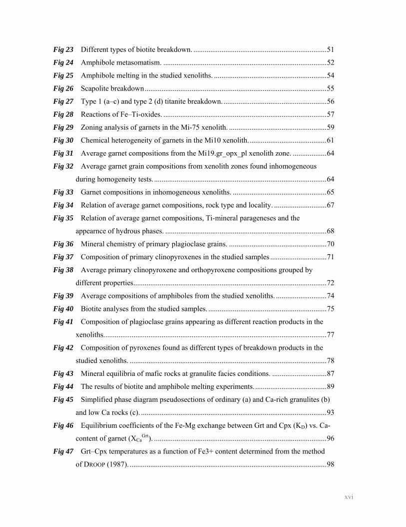
xvi
Fig 23 Different types of biotite breakdown. .......................................................................51
Fig 24 Amphibole metasomatism. .......................................................................................52
Fig 25 Amphibole melting in the studied xenoliths. ............................................................54
Fig 26 Scapolite breakdown.................................................................................................55
Fig 27 Type 1 (a–c) and type 2 (d) titanite breakdown. .......................................................56
Fig 28 Reactions of Fe–Ti-oxides. .......................................................................................57
Fig 29 Zoning analysis of garnets in the Mi-75 xenolith. ....................................................59
Fig 30 Chemical heterogeneity of garnets in the Mi10 xenolith..........................................61
Fig 31 Average garnet compositions from the Mi19.gr_opx_pl xenolith zone. ..................64
Fig 32 Average garnet grain compositions from xenolith zones found inhomogeneous
during homogeneity tests. ............................................................................................64
Fig 33 Garnet compositions in inhomogeneous xenoliths. ..................................................65
Fig 34 Relation of average garnet compositions, rock type and locality. ............................67
Fig 35 Relation of average garnet compositions, Ti-mineral parageneses and the
appearnce of hydrous phases. ......................................................................................68
Fig 36 Mineral chemistry of primary plagioclase grains. ....................................................70
Fig 37 Composition of primary clinopyroxenes in the studied samples ..............................71
Fig 38 Average primary clinopyroxene and orthopyroxene compositions grouped by
different properties.......................................................................................................72
Fig 39 Average compositions of amphiboles from the studied xenoliths. ...........................74
Fig 40 Biotite analyses from the studied samples. ...............................................................75
Fig 41 Composition of plagioclase grains appearing as different reaction products in the
xenoliths.......................................................................................................................77
Fig 42 Composition of pyroxenes found as different types of breakdown products in the
studied xenoliths. .........................................................................................................78
Fig 43 Mineral equilibria of mafic rocks at granulite facies conditions. .............................87
Fig 44 The results of biotite and amphibole melting experiments. ......................................89
Fig 45 Simplified phase diagram pseudosections of ordinary (a) and Ca-rich granulites (b)
and low Ca rocks (c). ...................................................................................................93
Fig 46 Equilibrium coefficients of the Fe-Mg exchange between Grt and Cpx (KD) vs. Ca-
content of garnet (XCaGrt). ............................................................................................96
Fig 47 Grt–Cpx temperatures as a function of Fe3+ content determined from the method
of DROOP (1987). .........................................................................................................98
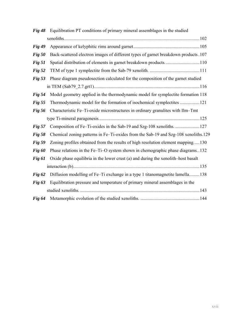
xvii
Fig 48 Equilibration PT conditions of primary mineral assemblages in the studied
xenoliths.....................................................................................................................102
Fig 49 Appearance of kelyphitic rims around garnet .........................................................105
Fig 50 Back-scattered electron images of different types of garnet breakdown products .107
Fig 51 Spatial distribution of elements in garnet breakdown products..............................110
Fig 52 TEM of type 1 symplectite from the Sab-79 xenolith. ...........................................111
Fig 53 Phase diagram pseudosection calculated for the composition of the garnet studied
in TEM (Sab79_2.7.grt1)...........................................................................................116
Fig 54 Model geometry applied in the thermodynamic model for symplectite formation 118
Fig 55 Thermodynamic model for the formation of isochemical symplectites .................121
Fig 56 Characteristic Fe–Ti-oxide microstructures in ordinary granulites with Ilm–Tmt
type Ti-mineral paragenesis.......................................................................................125
Fig 57 Composition of Fe–Ti-oxides in the Sab-19 and Szg-108 xenoliths. .....................127
Fig 58 Chemical zoning patterns in Fe–Ti-oxides from the Sab-19 and Szg-108 xenoliths.129
Fig 59 Zoning profiles obtained from the results of high resolution element mapping.....130
Fig 60 Phase relations in the Fe–Ti–O system shown in chemographic phase diagrams. .132
Fig 61 Oxide phase equilibria in the lower crust (a) and during the xenolith–host basalt
interaction (b).............................................................................................................135
Fig 62 Diffusion modelling of Fe–Ti exchange in a type 1 titanomagnetite lamella.........138
Fig 63 Equilibration pressure and temperature of primary mineral assemblages in the
studied xenoliths. .......................................................................................................143
Fig 64 Metamorphic evolution of the studied xenoliths. ...................................................144
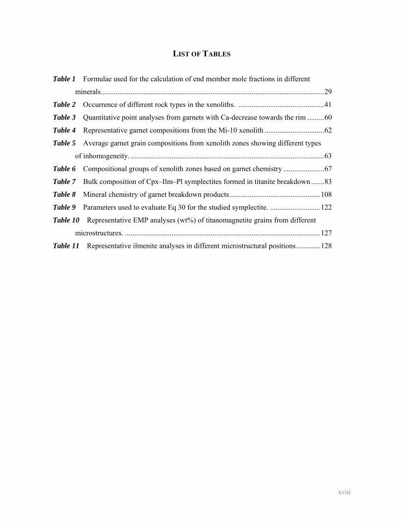
xviii
LIST OF TABLES
Table 1 Formulae used for the calculation of end member mole fractions in different
minerals........................................................................................................................29
Table 2 Occurrence of different rock types in the xenoliths. ..............................................41
Table 3 Quantitative point analyses from garnets with Ca-decrease towards the rim .........60
Table 4 Representative garnet compositions from the Mi-10 xenolith ................................62
Table 5 Average garnet grain compositions from xenolith zones showing different types
of inhomogeneity. ........................................................................................................63
Table 6 Compositional groups of xenolith zones based on garnet chemistry ......................67
Table 7 Bulk composition of Cpx–Ilm–Pl symplectites formed in titanite breakdown .......83
Table 8 Mineral chemistry of garnet breakdown products.................................................108
Table 9 Parameters used to evaluate Eq 30 for the studied symplectite. ...........................122
Table 10 Representative EMP analyses (wt%) of titanomagnetite grains from different
microstructures. .........................................................................................................127
Table 11 Representative ilmenite analyses in different microstructural positions.............128
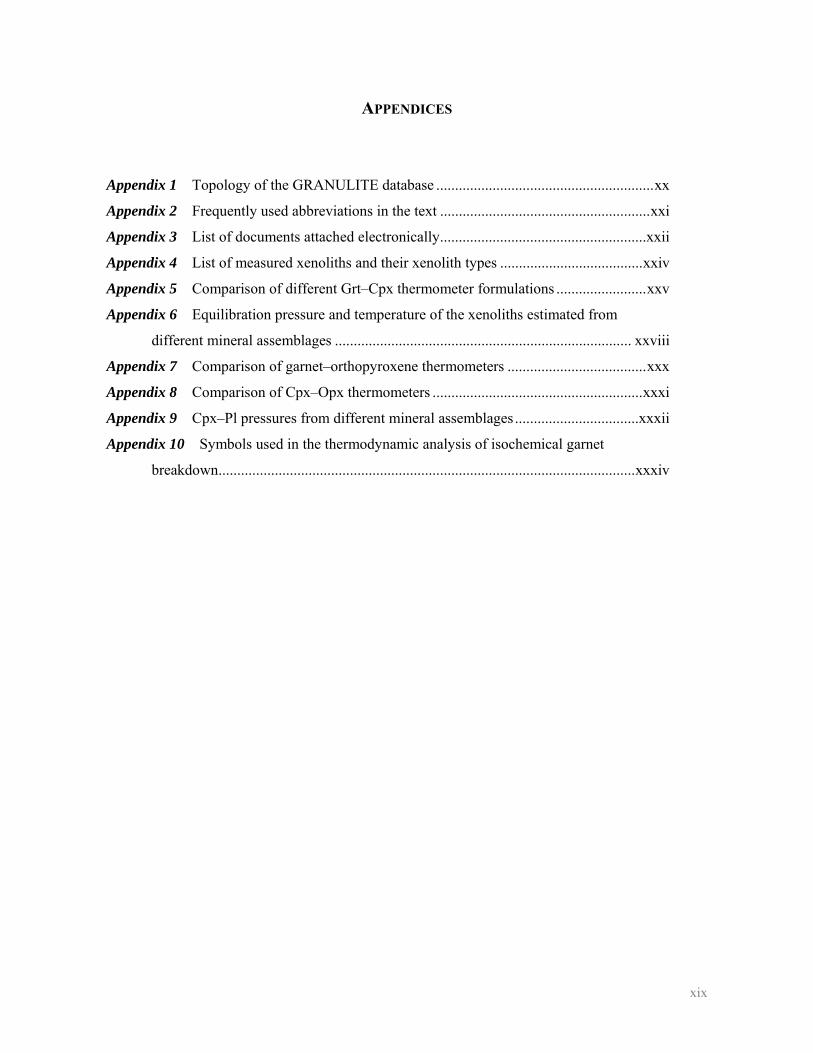
xix
APPENDICES
Appendix 1 Topology of the GRANULITE database ..........................................................xx
Appendix 2 Frequently used abbreviations in the text ........................................................xxi
Appendix 3 List of documents attached electronically.......................................................xxii
Appendix 4 List of measured xenoliths and their xenolith types ......................................xxiv
Appendix 5 Comparison of different Grt–Cpx thermometer formulations ........................xxv
Appendix 6 Equilibration pressure and temperature of the xenoliths estimated from
different mineral assemblages ............................................................................... xxviii
Appendix 7 Comparison of garnet–orthopyroxene thermometers .....................................xxx
Appendix 8 Comparison of Cpx–Opx thermometers ........................................................xxxi
Appendix 9 Cpx–Pl pressures from different mineral assemblages.................................xxxii
Appendix 10 Symbols used in the thermodynamic analysis of isochemical garnet
breakdown...............................................................................................................xxxiv
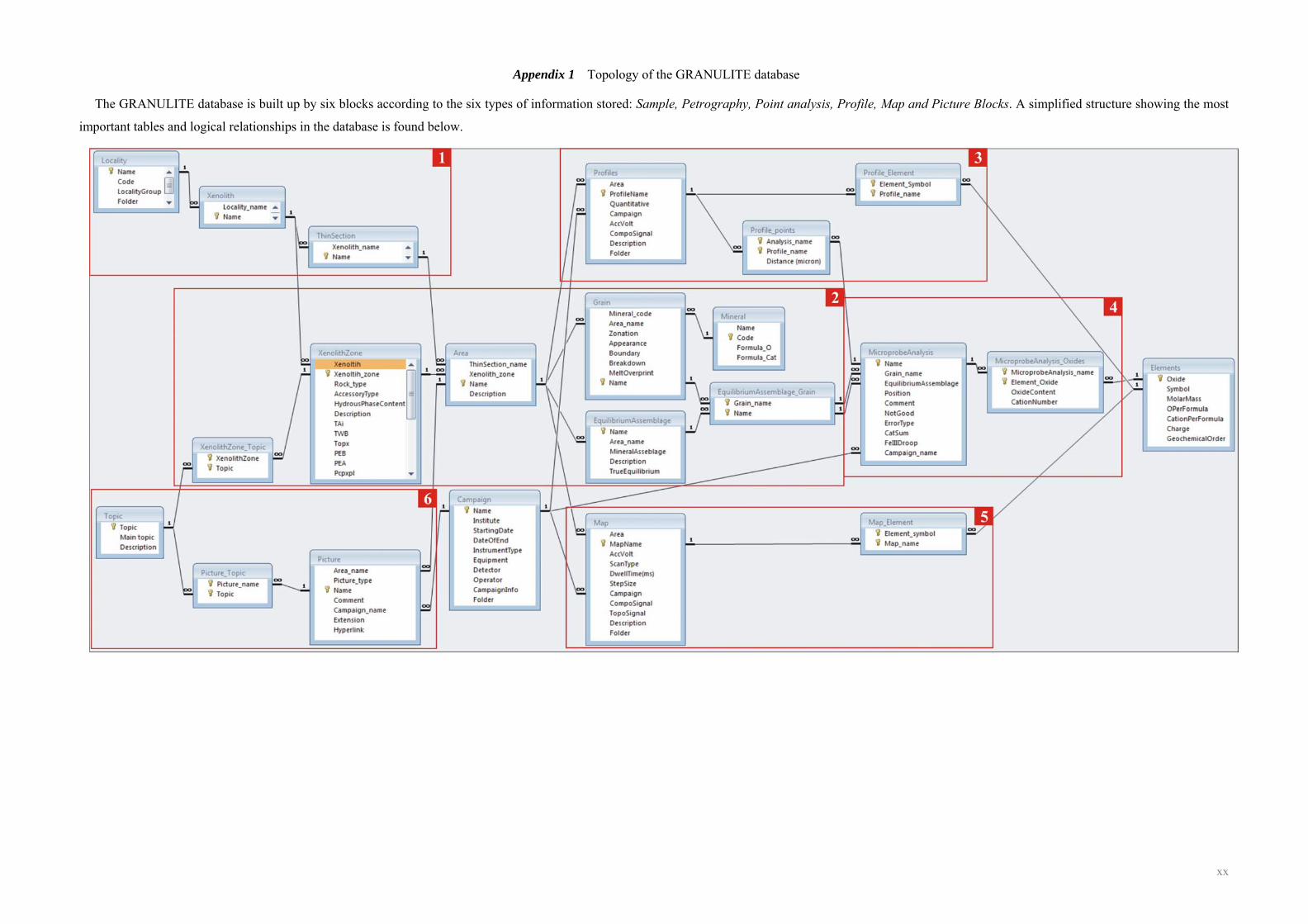
xx
Appendix 1 Topology of the GRANULITE database
The GRANULITE database is built up by six blocks according to the six types of information stored: Sample, Petrography, Point analysis, Profile, Map and Picture Blocks. A simplified structure showing the most
important tables and logical relationships in the database is found below.
xxi
Appendix 2 Frequently used abbreviations in the text
Mineral abbreviations follow Kretz (1983) modified by Spear (1995).
Amp amphibole
Ap apatite
Bt biotite
BBHVF Bakony–Balaton Highland Volcanic Field
CM crystallized melt
Cpx clinopyroxene
Gr graphite
Grt garnet
Ilm ilmenite
Kfs K-feldspar
Opx orthopyroxene
Pl plagioclase
Qtz quartz
Rt rutile
Scp scapolite
Smp symplectite after garnet
Ttn titanite
Zrn zircon
xxii
Appendix 3 List of documents attached electronically
File name Description
Petrography.pdf Petrography report of the GRANULITE database. All
petrographic observations together with the results of
geothermobarometry for each xenolith zone are summarized here.
GRANULITE.mdb The GRANULITE database described in Section III.
MineralChemistry_Grt.pdf Summary of quantitative point analyses and related mineral
chemical quantities from garnet grains studied in the thesis.
Report from the GRANULITE database.
MineralChemistry_Pl.pdf Summary of quantitative point analyses and related mineral
chemical quantities from plagioclase grains studied in the thesis.
Report from the GRANULITE database.
MineralChemistry_Cpx.pdf Summary of quantitative point analyses and related mineral
chemical quantities from clinopyroxene grains studied in the
thesis. Report from the GRANULITE database.
MineralChemistry_Opx.pdf Summary of quantitative point analyses and related mineral
chemical quantities from orthopyroxene grains studied in the
thesis. Report from the GRANULITE database.
MineralChemistry_Amp.pdf Summary of quantitative point analyses and related mineral
chemical quantities from amphibole grains studied in the thesis.
Report from the GRANULITE database.
MineralChemistry_Bt.pdf Summary of quantitative point analyses and related mineral
chemical quantities from biotite grains studied in the thesis.
Report from the GRANULITE database.
MineralChemistry_Scp.pdf Summary of quantitative point analyses and related mineral
chemical quantities from scapolite grains studied in the thesis.
Report from the GRANULITE database.
MineralChemistry_Ilm.pdf Summary of quantitative point analyses and related mineral
chemical quantities from ilmenite grains studied in the thesis.
Report from the GRANULITE database.
MineralChemistry_Mag.pdf Summary of quantitative point analyses and related mineral
chemical quantities from magnetite grains studied in the thesis.
Report from the GRANULITE database.
xxiii
MineralChemistry_Ol.pdf Summary of quantitative point analyses and related mineral
chemical quantities from olivine grains studied in the thesis.
Report from the GRANULITE database.
MineralChemistry_Spl.pdf Summary of quantitative point analyses and related mineral
chemical quantities from spinel grains studied in the thesis.
Report from the GRANULITE database.
Thermometers_Grt_Cpx.xls GTB workbook designed for the determination and comparison of
equilibrium temperatures from Grt–Cpx mineral pairs
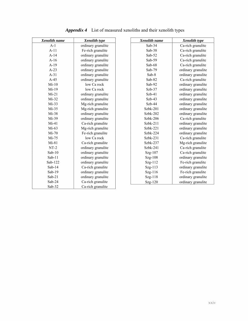
xxiv
Appendix 4 List of measured xenoliths and their xenolith types
Xenolith name Xenolith type A-1 ordinary granulite
A-11 Fe-rich granulite A-14 ordinary granulite A-16 ordinary granulite A-19 ordinary granulite A-23 ordinary granulite A-31 ordinary granulite A-45 ordinary granulite Mi-10 low Ca rock Mi-19 low Ca rock Mi-21 ordinary granulite Mi-32 ordinary granulite Mi-33 Mg-rich granulite Mi-35 Mg-rich granulite Mi-38 ordinary granulite Mi-39 ordinary granulite Mi-41 Ca-rich granulite Mi-63 Mg-rich granulite Mi-70 Fe-rich granulite Mi-75 low Ca rock Mi-81 Ca-rich granulite NT-2 ordinary granulite
Sab-10 ordinary granulite Sab-11 ordinary granulite Sab-122 ordinary granulite Sab-14 Ca-rich granulite Sab-19 ordinary granulite Sab-21 ordinary granulite Sab-24 Ca-rich granulite Sab-32 Ca-rich granulite
Xenolith name Xenolith type Sab-34 Ca-rich granulite Sab-38 Ca-rich granulite Sab-52 Ca-rich granulite Sab-59 Ca-rich granulite Sab-68 Ca-rich granulite Sab-79 ordinary granulite Sab-8 ordinary granulite Sab-82 Ca-rich granulite Sab-92 ordinary granulite Szb-37 ordinary granulite Szb-41 ordinary granulite Szb-43 ordinary granulite Szb-44 ordinary granulite
Szbk-201 ordinary granulite Szbk-202 ordinary granulite Szbk-206 Ca-rich granulite Szbk-211 ordinary granulite Szbk-221 ordinary granulite Szbk-224 ordinary granulite Szbk-231 Ca-rich granulite Szbk-237 Mg-rich granulite Szbk-241 Ca-rich granulite Szg-107 Ca-rich granulite Szg-108 ordinary granulite Szg-112 Fe-rich granulite Szg-113 ordinary granulite Szg-116 Fe-rich granulite Szg-118 ordinary granulite Szg-120 ordinary granulite
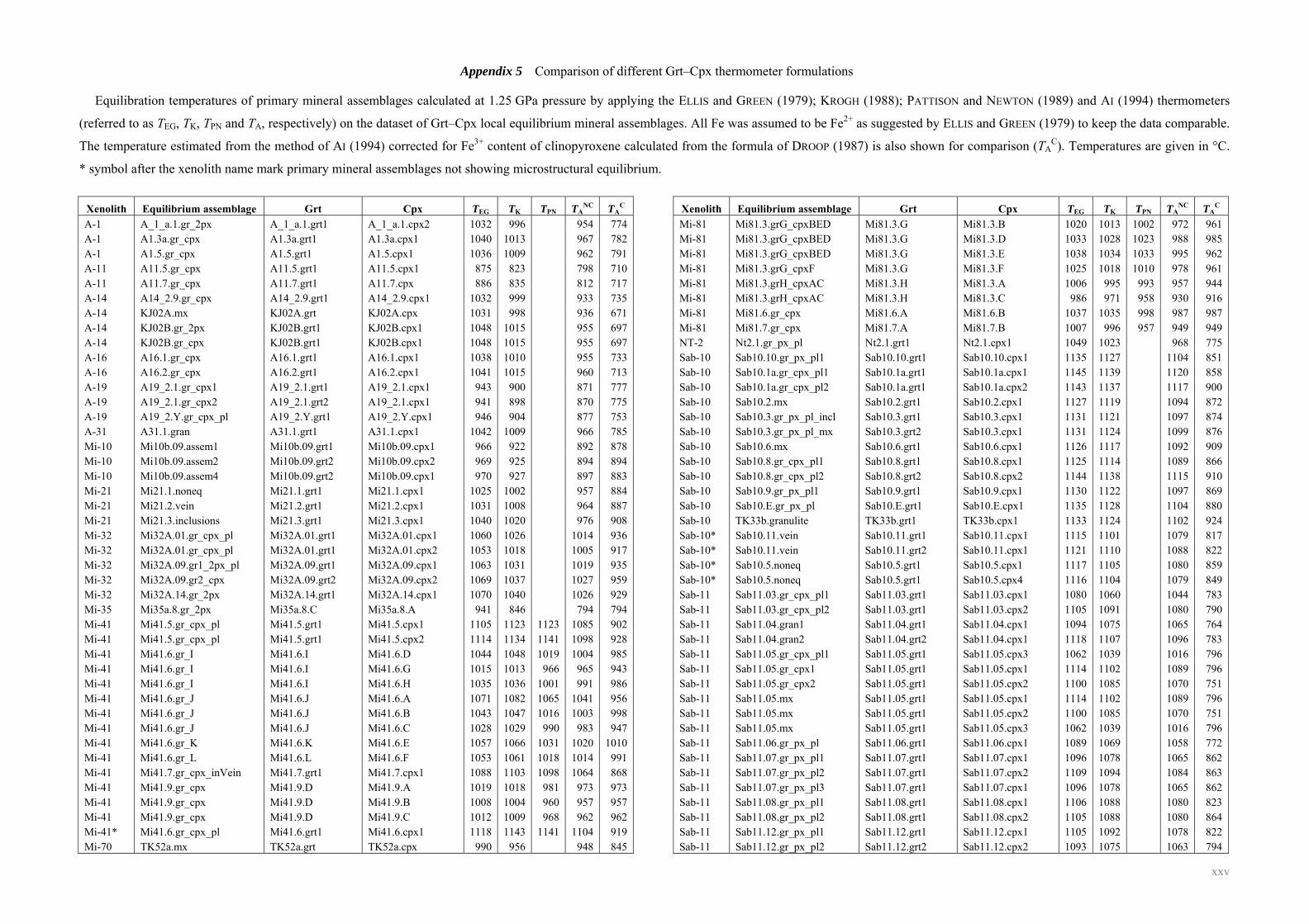
xxv
Appendix 5 Comparison of different Grt–Cpx thermometer formulations
Equilibration temperatures of primary mineral assemblages calculated at 1.25 GPa pressure by applying the ELLIS and GREEN (1979); KROGH (1988); PATTISON and NEWTON (1989) and AI (1994) thermometers
(referred to as TEG, TK, TPN and TA, respectively) on the dataset of Grt–Cpx local equilibrium mineral assemblages. All Fe was assumed to be Fe2+ as suggested by ELLIS and GREEN (1979) to keep the data comparable.
The temperature estimated from the method of AI (1994) corrected for Fe3+ content of clinopyroxene calculated from the formula of DROOP (1987) is also shown for comparison (TAC). Temperatures are given in °C.
* symbol after the xenolith name mark primary mineral assemblages not showing microstructural equilibrium.
Xenolith Equilibrium assemblage Grt Cpx TEG TK TPN TANC TA
C A-1 A_1_a.1.gr_2px A_1_a.1.grt1 A_1_a.1.cpx2 1032 996 954 774 A-1 A1.3a.gr_cpx A1.3a.grt1 A1.3a.cpx1 1040 1013 967 782 A-1 A1.5.gr_cpx A1.5.grt1 A1.5.cpx1 1036 1009 962 791 A-11 A11.5.gr_cpx A11.5.grt1 A11.5.cpx1 875 823 798 710 A-11 A11.7.gr_cpx A11.7.grt1 A11.7.cpx 886 835 812 717 A-14 A14_2.9.gr_cpx A14_2.9.grt1 A14_2.9.cpx1 1032 999 933 735 A-14 KJ02A.mx KJ02A.grt KJ02A.cpx 1031 998 936 671 A-14 KJ02B.gr_2px KJ02B.grt1 KJ02B.cpx1 1048 1015 955 697 A-14 KJ02B.gr_cpx KJ02B.grt1 KJ02B.cpx1 1048 1015 955 697 A-16 A16.1.gr_cpx A16.1.grt1 A16.1.cpx1 1038 1010 955 733 A-16 A16.2.gr_cpx A16.2.grt1 A16.2.cpx1 1041 1015 960 713 A-19 A19_2.1.gr_cpx1 A19_2.1.grt1 A19_2.1.cpx1 943 900 871 777 A-19 A19_2.1.gr_cpx2 A19_2.1.grt2 A19_2.1.cpx1 941 898 870 775 A-19 A19_2.Y.gr_cpx_pl A19_2.Y.grt1 A19_2.Y.cpx1 946 904 877 753 A-31 A31.1.gran A31.1.grt1 A31.1.cpx1 1042 1009 966 785 Mi-10 Mi10b.09.assem1 Mi10b.09.grt1 Mi10b.09.cpx1 966 922 892 878 Mi-10 Mi10b.09.assem2 Mi10b.09.grt2 Mi10b.09.cpx2 969 925 894 894 Mi-10 Mi10b.09.assem4 Mi10b.09.grt2 Mi10b.09.cpx1 970 927 897 883 Mi-21 Mi21.1.noneq Mi21.1.grt1 Mi21.1.cpx1 1025 1002 957 884 Mi-21 Mi21.2.vein Mi21.2.grt1 Mi21.2.cpx1 1031 1008 964 887 Mi-21 Mi21.3.inclusions Mi21.3.grt1 Mi21.3.cpx1 1040 1020 976 908 Mi-32 Mi32A.01.gr_cpx_pl Mi32A.01.grt1 Mi32A.01.cpx1 1060 1026 1014 936 Mi-32 Mi32A.01.gr_cpx_pl Mi32A.01.grt1 Mi32A.01.cpx2 1053 1018 1005 917 Mi-32 Mi32A.09.gr1_2px_pl Mi32A.09.grt1 Mi32A.09.cpx1 1063 1031 1019 935 Mi-32 Mi32A.09.gr2_cpx Mi32A.09.grt2 Mi32A.09.cpx2 1069 1037 1027 959 Mi-32 Mi32A.14.gr_2px Mi32A.14.grt1 Mi32A.14.cpx1 1070 1040 1026 929 Mi-35 Mi35a.8.gr_2px Mi35a.8.C Mi35a.8.A 941 846 794 794 Mi-41 Mi41.5.gr_cpx_pl Mi41.5.grt1 Mi41.5.cpx1 1105 1123 1123 1085 902 Mi-41 Mi41.5.gr_cpx_pl Mi41.5.grt1 Mi41.5.cpx2 1114 1134 1141 1098 928 Mi-41 Mi41.6.gr_I Mi41.6.I Mi41.6.D 1044 1048 1019 1004 985 Mi-41 Mi41.6.gr_I Mi41.6.I Mi41.6.G 1015 1013 966 965 943 Mi-41 Mi41.6.gr_I Mi41.6.I Mi41.6.H 1035 1036 1001 991 986 Mi-41 Mi41.6.gr_J Mi41.6.J Mi41.6.A 1071 1082 1065 1041 956 Mi-41 Mi41.6.gr_J Mi41.6.J Mi41.6.B 1043 1047 1016 1003 998 Mi-41 Mi41.6.gr_J Mi41.6.J Mi41.6.C 1028 1029 990 983 947 Mi-41 Mi41.6.gr_K Mi41.6.K Mi41.6.E 1057 1066 1031 1020 1010 Mi-41 Mi41.6.gr_L Mi41.6.L Mi41.6.F 1053 1061 1018 1014 991 Mi-41 Mi41.7.gr_cpx_inVein Mi41.7.grt1 Mi41.7.cpx1 1088 1103 1098 1064 868 Mi-41 Mi41.9.gr_cpx Mi41.9.D Mi41.9.A 1019 1018 981 973 973 Mi-41 Mi41.9.gr_cpx Mi41.9.D Mi41.9.B 1008 1004 960 957 957 Mi-41 Mi41.9.gr_cpx Mi41.9.D Mi41.9.C 1012 1009 968 962 962 Mi-41* Mi41.6.gr_cpx_pl Mi41.6.grt1 Mi41.6.cpx1 1118 1143 1141 1104 919 Mi-70 TK52a.mx TK52a.grt TK52a.cpx 990 956 948 845
Xenolith Equilibrium assemblage Grt Cpx TEG TK TPN TANC TA
C Mi-81 Mi81.3.grG_cpxBED Mi81.3.G Mi81.3.B 1020 1013 1002 972 961 Mi-81 Mi81.3.grG_cpxBED Mi81.3.G Mi81.3.D 1033 1028 1023 988 985 Mi-81 Mi81.3.grG_cpxBED Mi81.3.G Mi81.3.E 1038 1034 1033 995 962 Mi-81 Mi81.3.grG_cpxF Mi81.3.G Mi81.3.F 1025 1018 1010 978 961 Mi-81 Mi81.3.grH_cpxAC Mi81.3.H Mi81.3.A 1006 995 993 957 944 Mi-81 Mi81.3.grH_cpxAC Mi81.3.H Mi81.3.C 986 971 958 930 916 Mi-81 Mi81.6.gr_cpx Mi81.6.A Mi81.6.B 1037 1035 998 987 987 Mi-81 Mi81.7.gr_cpx Mi81.7.A Mi81.7.B 1007 996 957 949 949 NT-2 Nt2.1.gr_px_pl Nt2.1.grt1 Nt2.1.cpx1 1049 1023 968 775 Sab-10 Sab10.10.gr_px_pl1 Sab10.10.grt1 Sab10.10.cpx1 1135 1127 1104 851 Sab-10 Sab10.1a.gr_cpx_pl1 Sab10.1a.grt1 Sab10.1a.cpx1 1145 1139 1120 858 Sab-10 Sab10.1a.gr_cpx_pl2 Sab10.1a.grt1 Sab10.1a.cpx2 1143 1137 1117 900 Sab-10 Sab10.2.mx Sab10.2.grt1 Sab10.2.cpx1 1127 1119 1094 872 Sab-10 Sab10.3.gr_px_pl_incl Sab10.3.grt1 Sab10.3.cpx1 1131 1121 1097 874 Sab-10 Sab10.3.gr_px_pl_mx Sab10.3.grt2 Sab10.3.cpx1 1131 1124 1099 876 Sab-10 Sab10.6.mx Sab10.6.grt1 Sab10.6.cpx1 1126 1117 1092 909 Sab-10 Sab10.8.gr_cpx_pl1 Sab10.8.grt1 Sab10.8.cpx1 1125 1114 1089 866 Sab-10 Sab10.8.gr_cpx_pl2 Sab10.8.grt2 Sab10.8.cpx2 1144 1138 1115 910 Sab-10 Sab10.9.gr_px_pl1 Sab10.9.grt1 Sab10.9.cpx1 1130 1122 1097 869 Sab-10 Sab10.E.gr_px_pl Sab10.E.grt1 Sab10.E.cpx1 1135 1128 1104 880 Sab-10 TK33b.granulite TK33b.grt1 TK33b.cpx1 1133 1124 1102 924 Sab-10* Sab10.11.vein Sab10.11.grt1 Sab10.11.cpx1 1115 1101 1079 817 Sab-10* Sab10.11.vein Sab10.11.grt2 Sab10.11.cpx1 1121 1110 1088 822 Sab-10* Sab10.5.noneq Sab10.5.grt1 Sab10.5.cpx1 1117 1105 1080 859 Sab-10* Sab10.5.noneq Sab10.5.grt1 Sab10.5.cpx4 1116 1104 1079 849 Sab-11 Sab11.03.gr_cpx_pl1 Sab11.03.grt1 Sab11.03.cpx1 1080 1060 1044 783 Sab-11 Sab11.03.gr_cpx_pl2 Sab11.03.grt1 Sab11.03.cpx2 1105 1091 1080 790 Sab-11 Sab11.04.gran1 Sab11.04.grt1 Sab11.04.cpx1 1094 1075 1065 764 Sab-11 Sab11.04.gran2 Sab11.04.grt2 Sab11.04.cpx1 1118 1107 1096 783 Sab-11 Sab11.05.gr_cpx_pl1 Sab11.05.grt1 Sab11.05.cpx3 1062 1039 1016 796 Sab-11 Sab11.05.gr_cpx1 Sab11.05.grt1 Sab11.05.cpx1 1114 1102 1089 796 Sab-11 Sab11.05.gr_cpx2 Sab11.05.grt1 Sab11.05.cpx2 1100 1085 1070 751 Sab-11 Sab11.05.mx Sab11.05.grt1 Sab11.05.cpx1 1114 1102 1089 796 Sab-11 Sab11.05.mx Sab11.05.grt1 Sab11.05.cpx2 1100 1085 1070 751 Sab-11 Sab11.05.mx Sab11.05.grt1 Sab11.05.cpx3 1062 1039 1016 796 Sab-11 Sab11.06.gr_px_pl Sab11.06.grt1 Sab11.06.cpx1 1089 1069 1058 772 Sab-11 Sab11.07.gr_px_pl1 Sab11.07.grt1 Sab11.07.cpx1 1096 1078 1065 862 Sab-11 Sab11.07.gr_px_pl2 Sab11.07.grt1 Sab11.07.cpx2 1109 1094 1084 863 Sab-11 Sab11.07.gr_px_pl3 Sab11.07.grt1 Sab11.07.cpx1 1096 1078 1065 862 Sab-11 Sab11.08.gr_px_pl1 Sab11.08.grt1 Sab11.08.cpx1 1106 1088 1080 823 Sab-11 Sab11.08.gr_px_pl2 Sab11.08.grt1 Sab11.08.cpx2 1105 1088 1080 864 Sab-11 Sab11.12.gr_px_pl1 Sab11.12.grt1 Sab11.12.cpx1 1105 1092 1078 822 Sab-11 Sab11.12.gr_px_pl2 Sab11.12.grt2 Sab11.12.cpx2 1093 1075 1063 794
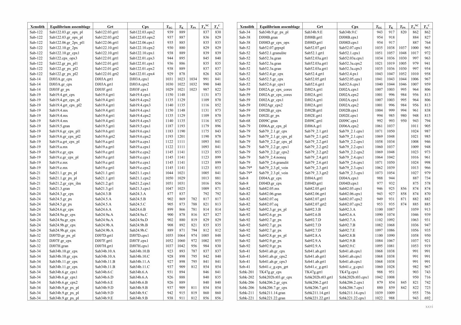
xxvi
Xenolith Equilibrium assemblage Grt Cpx TEG TK TPN TANC TA
C Sab-122 Sab122.03.gr_opx_pl Sab122.03.grt1 Sab122.03.opx2 939 889 837 830 Sab-122 Sab122.03.gr_opx_pl Sab122.03.grt2 Sab122.03.opx2 937 887 836 829 Sab-122 Sab122.06.gr_2px_pl1 Sab122.06.grt1 Sab122.06.cpx1 935 885 835 835 Sab-122 Sab122.10.gr_2px Sab122.10.grt1 Sab122.10.cpx2 930 880 829 829 Sab-122 Sab122.10.gr_cpx1 Sab122.10.grt1 Sab122.10.cpx1 938 889 839 839 Sab-122 Sab122.cpx_opx3 Sab122.01.grt1 Sab122.01.cpx3 944 895 845 840 Sab-122 Sab122.gr_px_pl1 Sab122.01.grt1 Sab122.01.cpx1 936 886 835 835 Sab-122 Sab122.gr_px_pl2 Sab122.01.grt2 Sab122.01.cpx2 938 889 837 837 Sab-122 Sab122.gr_px_pl2 Sab122.01.grt2 Sab122.01.cpx4 929 878 826 824 Sab-14 DJ03A.gr_cpx DJ03A.grt1 DJ03A.cpx1 1031 1023 1034 991 841 Sab-14 DJ03A.gr_cpx DJ03A.grt1 DJ03A.cpx2 1030 1022 1032 990 840 Sab-14 DJ03F.gr_px DJ03F.grt1 DJ03F.cpx1 1029 1021 1023 987 822 Sab-19 Sab19.4.grt_cpx Sab19.4.grt1 Sab19.4.cpx1 1150 1148 1131 873 Sab-19 Sab19.4.grt_cpx_pl Sab19.4.grt1 Sab19.4.cpx2 1135 1129 1109 870 Sab-19 Sab19.4.grt_cpx_pl2 Sab19.4.grt1 Sab19.4.cpx3 1140 1135 1116 852 Sab-19 Sab19.4.mx Sab19.4.grt1 Sab19.4.cpx1 1150 1148 1131 873 Sab-19 Sab19.4.mx Sab19.4.grt1 Sab19.4.cpx2 1135 1129 1109 870 Sab-19 Sab19.4.mx Sab19.4.grt1 Sab19.4.cpx3 1140 1135 1116 852 Sab-19 Sab19.5.gran Sab19.5.grt1 Sab19.5.cpx1 1187 1193 1179 896 Sab-19 Sab19.6.gr_cpx_pl1 Sab19.6.grt1 Sab19.6.cpx1 1183 1190 1175 843 Sab-19 Sab19.6.gr_cpx_pl2 Sab19.6.grt2 Sab19.6.cpx2 1193 1201 1190 878 Sab-19 Sab19.a.grt_cpx_pl Sab19.a.grt1 Sab19.a.cpx1 1122 1111 1093 841 Sab-19 Sab19.a.mx Sab19.a.grt1 Sab19.a.cpx1 1122 1111 1093 841 Sab-19 Sab19.e.gr_cpx Sab19.e.grt1 Sab19.e.cpx2 1145 1141 1123 853 Sab-19 Sab19.e.gr_cpx_pl Sab19.e.grt1 Sab19.e.cpx1 1145 1141 1123 899 Sab-19 Sab19.e.mx Sab19.e.grt1 Sab19.e.cpx1 1145 1141 1123 899 Sab-19 Sab19.e.mx Sab19.e.grt1 Sab19.e.cpx2 1145 1141 1123 853 Sab-21 Sab21.1.gr_px_pl Sab21.1.grt1 Sab21.1.cpx1 1044 1021 1005 841 Sab-21 Sab21.1.gr_px_pl Sab21.1.grt1 Sab21.1.cpx2 1050 1029 1013 881 Sab-21 Sab21.2.gr_cpx_ilm Sab21.2.gr1 Sab21.2.cpx1 1051 1031 1016 856 Sab-21 Sab21.3.gran Sab21.3.gr1 Sab21.3.cpx1 1047 1025 1009 871 Sab-24 Sab24.3.gr_cpx Sab24.3.B Sab24.3.A 877 837 792 792 Sab-24 Sab24.5.gr_px Sab24.5.A Sab24.5.B 902 869 782 817 817 Sab-24 Sab24.5.gr_px Sab24.5.A Sab24.5.C 905 873 788 821 813 Sab-24 Sab24.6.gr_cpx Sab24.6.A Sab24.6.B 899 866 781 814 814 Sab-24 Sab24.9a.gr_cpx Sab24.9a.A Sab24.9a.C 900 878 816 827 827 Sab-24 Sab24.9a.gr_cpx Sab24.9a.A Sab24.9a.D 902 880 819 829 829 Sab-24 Sab24.9b.gr_cpx Sab24.9b.A Sab24.9b.B 908 892 821 835 835 Sab-24 Sab24.9b.gr_cpx Sab24.9b.A Sab24.9b.C 889 871 794 812 812 Sab-32 DJ07D.gr_px_pl DJ07D.grt1 DJ07D.cpx1 1055 1064 974 1005 848 Sab-32 DJ07F.gr_cpx DJ07F.grt1 DJ07F.cpx1 1052 1060 972 1002 855 Sab-32 DJ07H.gran DJ07H.grt1 DJ07H.cpx1 1037 1042 956 984 830 Sab-34 Sab34b.10.gr_cpx Sab34b.10.A Sab34b.10.B 923 893 787 837 837 Sab-34 Sab34b.10.gr_cpx Sab34b.10.A Sab34b.10.C 928 898 795 842 840 Sab-34 Sab34b.11.gr_cpx Sab34b.11.B Sab34b.11.A 927 898 795 841 841 Sab-34 Sab34b.11.gr_cpx Sab34b.11.B Sab34b.11.C 937 909 812 854 854 Sab-34 Sab34b.6.gr_cpx1 Sab34b.6.C Sab34b.6.A 931 894 846 841 Sab-34 Sab34b.6.gr_cpx1 Sab34b.6.D Sab34b.6.A 926 888 840 835 Sab-34 Sab34b.6.gr_cpx2 Sab34b.6.E Sab34b.6.B 926 889 840 840 Sab-34 Sab34b.9.gr_px_pl Sab34b.9.D Sab34b.9.B 937 909 811 854 854 Sab-34 Sab34b.9.gr_px_pl Sab34b.9.D Sab34b.9.C 942 915 819 860 860 Sab-34 Sab34b.9.gr_px_pl Sab34b.9.E Sab34b.9.B 938 911 812 856 856
Xenolith Equilibrium assemblage Grt Cpx TEG TK TPN TANC TA
C Sab-34 Sab34b.9.gr_px_pl Sab34b.9.E Sab34b.9.C 943 917 820 862 862 Sab-38 DJ08B.gran DJ08B.grt1 DJ08B.cpx1 954 918 884 827 Sab-38 DJ08D.gr_cpx_opx DJ08D.grt1 DJ08D.cpx1 954 917 887 764 Sab-52 Sab52.07.grpxpl Sab52.07.grt1 Sab52.07.cpx1 1035 1038 1037 1000 965 Sab-52 Sab52.1.granulite Sab52.1.grt1 Sab52.1.cpx1 1051 1057 1048 1017 972 Sab-52 Sab52.3a.gran Sab52.03a.grt1 Sab52.03a.cpx1 1034 1036 1030 997 963 Sab-52 Sab52.3a.gran Sab52.03a.grt1 Sab52.3a.cpx2 1021 1019 1005 979 941 Sab-52 Sab52.3a.gran Sab52.03a.grt1 Sab52.3a.cpx3 1035 1036 1030 997 954 Sab-52 Sab52.4.gr_cpx Sab52.4.grt1 Sab52.4.px1 1043 1047 1052 1010 958 Sab-52 Sab52.5.gr_cpx Sab52.05.grt1 Sab52.05.cpx1 1041 1043 1044 1006 967 Sab-52 Sab52.6.gr_cpx1 Sab52.6.grt1 Sab52.6.cpx1 1040 1044 1046 1007 959 Sab-59 DJ02A.gr_cpx_cores DJ02A.grt1 DJ02A.cpx1 1007 1003 995 964 806 Sab-59 DJ02A.gr_cpx_cores DJ02A.grt1 DJ02A.cpx2 1001 996 984 956 813 Sab-59 DJ02A.gr_cpx1 DJ02A.grt1 DJ02A.cpx1 1007 1003 995 964 806 Sab-59 DJ02Agr_cpx2 DJ02A.grt1 DJ02A.cpx2 1001 996 984 956 813 Sab-59 DJ02B.gr_cpx DJ02B.grt1 DJ02B.cpx1 1004 999 994 961 838 Sab-59 DJ02E.gr_px DJ02E.grt1 DJ02E.cpx1 994 985 980 948 815 Sab-68 DJ09C.gran DJ09C.grt1 DJ09C.cpx1 992 993 950 943 794 Sab-79 DJ06A.gr_cpx_pl DJ06A.gr1 DJ06A.cpx2 1061 1037 1011 905 Sab-79 Sab79_2.1.gr_cpx Sab79_2.1.grt1 Sab79_2.1.cpx1 1071 1050 1024 987 Sab-79 Sab79_2.1.gr_cpx_pl Sab79_2.1.grt2 Sab79_2.1.cpx1 1069 1048 1021 985 Sab-79 Sab79_2.2.gr_cpx_pl Sab79_2.2.grt1 Sab79_2.2.cpx1 1058 1034 1008 946 Sab-79 Sab79_2.2.gr_cpx1 Sab79_2.2.grt2 Sab79_2.2.cpx1 1060 1037 1009 948 Sab-79 Sab79_2.2.gr_cpx2 Sab79_2.2.grt2 Sab79_2.2.cpx2 1069 1048 1023 973 Sab-79 Sab79_2.4.noneq Sab79_2.4.grt1 Sab79_2.4.cpx1 1064 1042 1016 961 Sab-79 Sab79_2.6.granulit Sab79_2.6.grt1 Sab79_2.6.cpx1 1071 1050 1024 998 Sab-79* Sab79_2.3.pl_vein Sab79_2.3.grt1 Sab79_2.3.cpx1 1062 1039 1013 966 Sab-79* Sab79_2.3.pl_vein Sab79_2.3.grt2 Sab79_2.3.cpx1 1073 1054 1027 979 Sab-8 DJ04A.gr_cpx DJ04A.grt1 DJ04A.cpx1 988 944 887 734 Sab-8 DJ04D.gr_cpx DJ04D.grt1 DJ04D.cpx1 977 932 875 578 Sab-82 Sab82.05.mx Sab82.05.grt1 Sab82.05.cpx1 946 925 856 874 874 Sab-82 Sab82.06.gran Sab82.06.grt1 Sab82.06.cpx1 943 927 858 874 870 Sab-82 Sab82.07.eq Sab82.07.grt1 Sab82.07.cpx2 949 931 871 882 882 Sab-82 Sab82.07.eq Sab82.07.grt2 Sab82.07.cpx2 953 935 874 885 885 Sab-92 Sab92.3.gr_px_pl Sab92.3.B Sab92.3.A 1100 1087 1059 913 Sab-92 Sab92.6.gr_px Sab92.6.B Sab92.6.A 1090 1074 1046 939 Sab-92 Sab92.7.gr_px Sab92.7.D Sab92.7.A 1102 1092 1063 931 Sab-92 Sab92.7.gr_px Sab92.7.D Sab92.7.B 1082 1068 1036 947 Sab-92 Sab92.7.gr_px Sab92.7.D Sab92.7.E 1097 1086 1056 935 Sab-92 Sab92.8.gr_px_pl Sab92.8.A Sab92.8.B 1100 1090 1058 950 Sab-92 Sab92.9.gr_px Sab92.9.A Sab92.9.B 1084 1067 1037 921 Sab-92 Sab92.9.gr_px Sab92.9.A Sab92.9.C 1095 1081 1053 919 Szb-41 Szb41.ab.gr_cpx Szb41.ab.grt1 Szb41.ab.cpx1 1068 1038 991 991 Szb-41 Szb41.ab.gr_cpx2 Szb41.ab.grt1 Szb41.ab.cpx1 1068 1038 991 991 Szb-41 Szb41.ab.gr_cpx3 Szb41.ab.grt1 Szb41.ab.cpx1 1068 1038 991 991 Szb-41 Szb41.c_g.cpx_grt Szb41.c_g.grt1 Szb41.c_g.cpx1 1060 1028 982 967 Szbk-201 TK47g.gr_cpx TK47g.grt1 TK47g.cpx1 988 951 903 743 Szbk-202 Szbk202b.t03.gr_cpx Szbk202b.t03.grt1 Szbk202b.t03.cpx1 1042 1008 950 716 Szbk-206 Szbk206.2.gr_cpx Szbk206.2.grt1 Szbk206.2.cpx1 879 854 845 821 742 Szbk-206 Szbk206.7.gr_cpx Szbk206.7.grt1 Szbk206.7.cpx1 880 859 842 822 723 Szbk-211 Szbk211.14.gran Szbk211.14.grt1 Szbk211.14.cpx1 1039 1009 955 756 Szbk-221 Szbk221.22.gran Szbk221.22.grt1 Szbk221.22.cpx1 1022 988 943 692
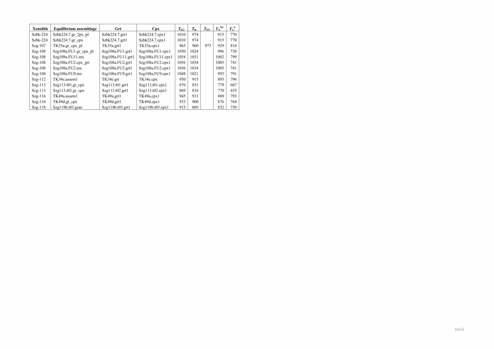
xxvii
Xenolith Equilibrium assemblage Grt Cpx TEG TK TPN TANC TA
C Szbk-224 Szbk224.7.gr_2px_pl Szbk224.7.grt1 Szbk224.7.cpx1 1010 974 915 770 Szbk-224 Szbk224.7.gr_cpx Szbk224.7.grt1 Szbk224.7.cpx1 1010 974 915 770 Szg-107 TK35a.gr_cpx_pl TK35a.grt1 TK35a.cpx1 965 960 973 929 816 Szg-108 Szg108a.FU1.gr_cpx_pl Szg108a.FU1.grt1 Szg108a.FU1.cpx1 1050 1024 996 738 Szg-108 Szg108a.FU11.mx Szg108a.FU11.grt1 Szg108a.FU11.cpx1 1054 1031 1002 799 Szg-108 Szg108a.FU2.cpx_grt Szg108a.FU2.grt1 Szg108a.FU2.cpx1 1056 1034 1005 741 Szg-108 Szg108a.FU2.mx Szg108a.FU2.grt1 Szg108a.FU2.cpx1 1056 1034 1005 741 Szg-108 Szg108a.FU9.mx Szg108a.FU9.grt1 Szg108a.FU9.cpx1 1048 1021 993 791 Szg-112 TK34e.assem1 TK34e.grt TK34e.cpx 950 915 895 796 Szg-113 Szg113.t01.gr_cpx Szg113.t01.grt1 Szg113.t01.cpx1 876 831 779 667 Szg-113 Szg113.t02.gr_cpx Szg113.t02.grt1 Szg113.t02.cpx1 869 816 770 655 Szg-116 TK49a.assem1 TK49a.grt1 TK49a.cpx1 945 913 889 793 Szg-116 TK49d.gr_cpx TK49d.grt1 TK49d.cpx1 933 900 876 764 Szg-118 Szg118b.t03.gran Szg118b.t03.grt1 Szg118b.t03.cpx1 915 869 832 750
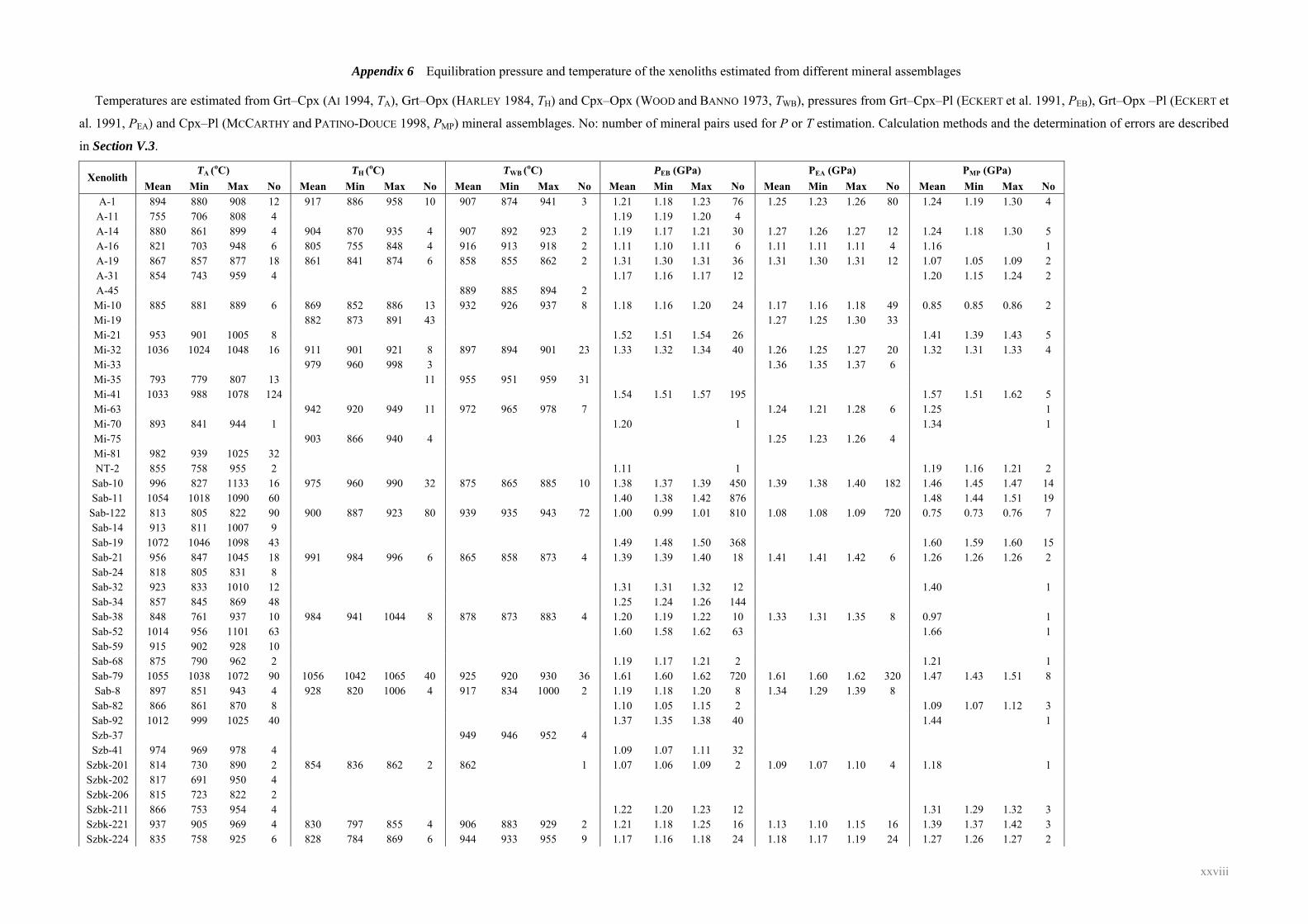
xxviii
Appendix 6 Equilibration pressure and temperature of the xenoliths estimated from different mineral assemblages
Temperatures are estimated from Grt–Cpx (AI 1994, TA), Grt–Opx (HARLEY 1984, TH) and Cpx–Opx (WOOD and BANNO 1973, TWB), pressures from Grt–Cpx–Pl (ECKERT et al. 1991, PEB), Grt–Opx –Pl (ECKERT et
al. 1991, PEA) and Cpx–Pl (MCCARTHY and PATINO-DOUCE 1998, PMP) mineral assemblages. No: number of mineral pairs used for P or T estimation. Calculation methods and the determination of errors are described
in Section V.3.
TA (oC) TH (oC) TWB (oC) PEB (GPa) PEA (GPa) PMP (GPa) Xenolith Mean Min Max No Mean Min Max No Mean Min Max No Mean Min Max No Mean Min Max No Mean Min Max No
A-1 894 880 908 12 917 886 958 10 907 874 941 3 1.21 1.18 1.23 76 1.25 1.23 1.26 80 1.24 1.19 1.30 4 A-11 755 706 808 4 1.19 1.19 1.20 4 A-14 880 861 899 4 904 870 935 4 907 892 923 2 1.19 1.17 1.21 30 1.27 1.26 1.27 12 1.24 1.18 1.30 5 A-16 821 703 948 6 805 755 848 4 916 913 918 2 1.11 1.10 1.11 6 1.11 1.11 1.11 4 1.16 1 A-19 867 857 877 18 861 841 874 6 858 855 862 2 1.31 1.30 1.31 36 1.31 1.30 1.31 12 1.07 1.05 1.09 2 A-31 854 743 959 4 1.17 1.16 1.17 12 1.20 1.15 1.24 2 A-45 889 885 894 2 Mi-10 885 881 889 6 869 852 886 13 932 926 937 8 1.18 1.16 1.20 24 1.17 1.16 1.18 49 0.85 0.85 0.86 2 Mi-19 882 873 891 43 1.27 1.25 1.30 33 Mi-21 953 901 1005 8 1.52 1.51 1.54 26 1.41 1.39 1.43 5 Mi-32 1036 1024 1048 16 911 901 921 8 897 894 901 23 1.33 1.32 1.34 40 1.26 1.25 1.27 20 1.32 1.31 1.33 4 Mi-33 979 960 998 3 1.36 1.35 1.37 6 Mi-35 793 779 807 13 11 955 951 959 31 Mi-41 1033 988 1078 124 1.54 1.51 1.57 195 1.57 1.51 1.62 5 Mi-63 942 920 949 11 972 965 978 7 1.24 1.21 1.28 6 1.25 1 Mi-70 893 841 944 1 1.20 1 1.34 1 Mi-75 903 866 940 4 1.25 1.23 1.26 4 Mi-81 982 939 1025 32 NT-2 855 758 955 2 1.11 1 1.19 1.16 1.21 2
Sab-10 996 827 1133 16 975 960 990 32 875 865 885 10 1.38 1.37 1.39 450 1.39 1.38 1.40 182 1.46 1.45 1.47 14 Sab-11 1054 1018 1090 60 1.40 1.38 1.42 876 1.48 1.44 1.51 19
Sab-122 813 805 822 90 900 887 923 80 939 935 943 72 1.00 0.99 1.01 810 1.08 1.08 1.09 720 0.75 0.73 0.76 7 Sab-14 913 811 1007 9 Sab-19 1072 1046 1098 43 1.49 1.48 1.50 368 1.60 1.59 1.60 15 Sab-21 956 847 1045 18 991 984 996 6 865 858 873 4 1.39 1.39 1.40 18 1.41 1.41 1.42 6 1.26 1.26 1.26 2 Sab-24 818 805 831 8 Sab-32 923 833 1010 12 1.31 1.31 1.32 12 1.40 1 Sab-34 857 845 869 48 1.25 1.24 1.26 144 Sab-38 848 761 937 10 984 941 1044 8 878 873 883 4 1.20 1.19 1.22 10 1.33 1.31 1.35 8 0.97 1 Sab-52 1014 956 1101 63 1.60 1.58 1.62 63 1.66 1 Sab-59 915 902 928 10 Sab-68 875 790 962 2 1.19 1.17 1.21 2 1.21 1 Sab-79 1055 1038 1072 90 1056 1042 1065 40 925 920 930 36 1.61 1.60 1.62 720 1.61 1.60 1.62 320 1.47 1.43 1.51 8 Sab-8 897 851 943 4 928 820 1006 4 917 834 1000 2 1.19 1.18 1.20 8 1.34 1.29 1.39 8 Sab-82 866 861 870 8 1.10 1.05 1.15 2 1.09 1.07 1.12 3 Sab-92 1012 999 1025 40 1.37 1.35 1.38 40 1.44 1 Szb-37 949 946 952 4 Szb-41 974 969 978 4 1.09 1.07 1.11 32
Szbk-201 814 730 890 2 854 836 862 2 862 1 1.07 1.06 1.09 2 1.09 1.07 1.10 4 1.18 1 Szbk-202 817 691 950 4 Szbk-206 815 723 822 2 Szbk-211 866 753 954 4 1.22 1.20 1.23 12 1.31 1.29 1.32 3 Szbk-221 937 905 969 4 830 797 855 4 906 883 929 2 1.21 1.18 1.25 16 1.13 1.10 1.15 16 1.39 1.37 1.42 3 Szbk-224 835 758 925 6 828 784 869 6 944 933 955 9 1.17 1.16 1.18 24 1.18 1.17 1.19 24 1.27 1.26 1.27 2
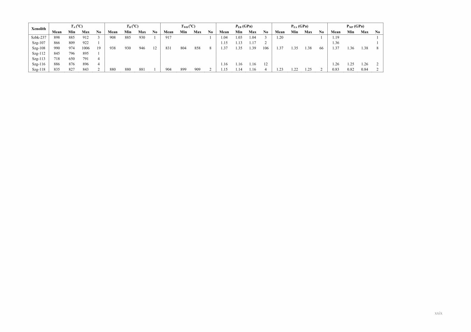
xxix
TA (oC) TH (oC) TWB (oC) PEB (GPa) PEA (GPa) PMP (GPa) Xenolith Mean Min Max No Mean Min Max No Mean Min Max No Mean Min Max No Mean Min Max No Mean Min Max No
Szbk-237 898 885 912 3 908 885 930 1 917 1 1.04 1.03 1.04 3 1.20 1 1.19 1 Szg-107 866 809 922 1 1.15 1.13 1.17 2 1.36 1 Szg-108 990 974 1006 19 938 930 946 12 831 804 858 8 1.37 1.35 1.39 106 1.37 1.35 1.38 66 1.37 1.36 1.38 8 Szg-112 845 796 895 1 Szg-113 718 650 791 4 Szg-116 886 876 896 4 1.16 1.16 1.16 12 1.26 1.25 1.26 2 Szg-118 835 827 843 2 880 880 881 1 904 899 909 2 1.15 1.14 1.16 4 1.23 1.22 1.25 2 0.83 0.82 0.84 2
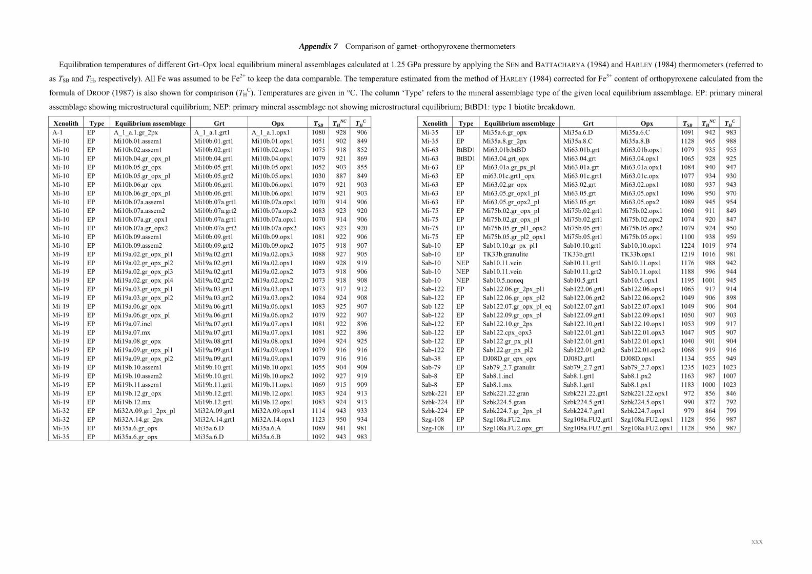
xxx
Appendix 7 Comparison of garnet–orthopyroxene thermometers
Equilibration temperatures of different Grt–Opx local equilibrium mineral assemblages calculated at 1.25 GPa pressure by applying the SEN and BATTACHARYA (1984) and HARLEY (1984) thermometers (referred to
as TSB and TH, respectively). All Fe was assumed to be Fe2+ to keep the data comparable. The temperature estimated from the method of HARLEY (1984) corrected for Fe3+ content of orthopyroxene calculated from the
formula of DROOP (1987) is also shown for comparison (THC). Temperatures are given in °C. The column ‘Type’ refers to the mineral assemblage type of the given local equilibrium assemblage. EP: primary mineral
assemblage showing microstructural equilibrium; NEP: primary mineral assemblage not showing microstructural equilibrium; BtBD1: type 1 biotite breakdown.
Xenolith Type Equilibrium assemblage Grt Opx TSB THNC TH
C A-1 EP A_1_a.1.gr_2px A_1_a.1.grt1 A_1_a.1.opx1 1080 928 906 Mi-10 EP Mi10b.01.assem1 Mi10b.01.grt1 Mi10b.01.opx1 1051 902 849 Mi-10 EP Mi10b.02.assem1 Mi10b.02.grt1 Mi10b.02.opx1 1075 918 852 Mi-10 EP Mi10b.04.gr_opx_pl Mi10b.04.grt1 Mi10b.04.opx1 1079 921 869 Mi-10 EP Mi10b.05.gr_opx Mi10b.05.grt1 Mi10b.05.opx1 1052 903 855 Mi-10 EP Mi10b.05.gr_opx_pl Mi10b.05.grt2 Mi10b.05.opx1 1030 887 849 Mi-10 EP Mi10b.06.gr_opx Mi10b.06.grt1 Mi10b.06.opx1 1079 921 903 Mi-10 EP Mi10b.06.gr_opx_pl Mi10b.06.grt1 Mi10b.06.opx1 1079 921 903 Mi-10 EP Mi10b.07a.assem1 Mi10b.07a.grt1 Mi10b.07a.opx1 1070 914 906 Mi-10 EP Mi10b.07a.assem2 Mi10b.07a.grt2 Mi10b.07a.opx2 1083 923 920 Mi-10 EP Mi10b.07a.gr_opx1 Mi10b.07a.grt1 Mi10b.07a.opx1 1070 914 906 Mi-10 EP Mi10b.07a.gr_opx2 Mi10b.07a.grt2 Mi10b.07a.opx2 1083 923 920 Mi-10 EP Mi10b.09.assem1 Mi10b.09.grt1 Mi10b.09.opx1 1081 922 906 Mi-10 EP Mi10b.09.assem2 Mi10b.09.grt2 Mi10b.09.opx2 1075 918 907 Mi-19 EP Mi19a.02.gr_opx_pl1 Mi19a.02.grt1 Mi19a.02.opx3 1088 927 905 Mi-19 EP Mi19a.02.gr_opx_pl2 Mi19a.02.grt1 Mi19a.02.opx1 1089 928 919 Mi-19 EP Mi19a.02.gr_opx_pl3 Mi19a.02.grt1 Mi19a.02.opx2 1073 918 906 Mi-19 EP Mi19a.02.gr_opx_pl4 Mi19a.02.grt2 Mi19a.02.opx2 1073 918 908 Mi-19 EP Mi19a.03.gr_opx_pl1 Mi19a.03.grt1 Mi19a.03.opx1 1073 917 912 Mi-19 EP Mi19a.03.gr_opx_pl2 Mi19a.03.grt2 Mi19a.03.opx2 1084 924 908 Mi-19 EP Mi19a.06.gr_opx Mi19a.06.grt1 Mi19a.06.opx1 1083 925 907 Mi-19 EP Mi19a.06.gr_opx_pl Mi19a.06.grt1 Mi19a.06.opx2 1079 922 907 Mi-19 EP Mi19a.07.incl Mi19a.07.grt1 Mi19a.07.opx1 1081 922 896 Mi-19 EP Mi19a.07.mx Mi19a.07.grt1 Mi19a.07.opx1 1081 922 896 Mi-19 EP Mi19a.08.gr_opx Mi19a.08.grt1 Mi19a.08.opx1 1094 924 925 Mi-19 EP Mi19a.09.gr_opx_pl1 Mi19a.09.grt1 Mi19a.09.opx1 1079 916 916 Mi-19 EP Mi19a.09.gr_opx_pl2 Mi19a.09.grt1 Mi19a.09.opx1 1079 916 916 Mi-19 EP Mi19b.10.assem1 Mi19b.10.grt1 Mi19b.10.opx1 1055 904 909 Mi-19 EP Mi19b.10.assem2 Mi19b.10.grt1 Mi19b.10.opx2 1092 927 919 Mi-19 EP Mi19b.11.assem1 Mi19b.11.grt1 Mi19b.11.opx1 1069 915 909 Mi-19 EP Mi19b.12.gr_opx Mi19b.12.grt1 Mi19b.12.opx1 1083 924 913 Mi-19 EP Mi19b.12.mx Mi19b.12.grt1 Mi19b.12.opx1 1083 924 913 Mi-32 EP Mi32A.09.gr1_2px_pl Mi32A.09.grt1 Mi32A.09.opx1 1114 943 933 Mi-32 EP Mi32A.14.gr_2px Mi32A.14.grt1 Mi32A.14.opx1 1123 950 934 Mi-35 EP Mi35a.6.gr_opx Mi35a.6.D Mi35a.6.A 1089 941 981 Mi-35 EP Mi35a.6.gr_opx Mi35a.6.D Mi35a.6.B 1092 943 983
Xenolith Type Equilibrium assemblage Grt Opx TSB THNC TH
C Mi-35 EP Mi35a.6.gr_opx Mi35a.6.D Mi35a.6.C 1091 942 983 Mi-35 EP Mi35a.8.gr_2px Mi35a.8.C Mi35a.8.B 1128 965 988 Mi-63 BtBD1 Mi63.01b.btBD Mi63.01b.grt Mi63.01b.opx1 1079 935 955 Mi-63 BtBD1 Mi63.04.grt_opx Mi63.04.grt Mi63.04.opx1 1065 928 925 Mi-63 EP Mi63.01a.gr_px_pl Mi63.01a.grt Mi63.01a.opx1 1084 940 947 Mi-63 EP mi63.01c.grt1_opx Mi63.01c.grt1 Mi63.01c.opx 1077 934 930 Mi-63 EP Mi63.02.gr_opx Mi63.02.grt Mi63.02.opx1 1080 937 943 Mi-63 EP Mi63.05.gr_opx1_pl Mi63.05.grt Mi63.05.opx1 1096 950 970 Mi-63 EP Mi63.05.gr_opx2_pl Mi63.05.grt Mi63.05.opx2 1089 945 954 Mi-75 EP Mi75b.02.gr_opx_pl Mi75b.02.grt1 Mi75b.02.opx1 1060 911 849 Mi-75 EP Mi75b.02.gr_opx_pl Mi75b.02.grt1 Mi75b.02.opx2 1074 920 847 Mi-75 EP Mi75b.05.gr_pl1_opx2 Mi75b.05.grt1 Mi75b.05.opx2 1079 924 950 Mi-75 EP Mi75b.05.gr_pl2_opx1 Mi75b.05.grt1 Mi75b.05.opx1 1100 938 959 Sab-10 EP Sab10.10.gr_px_pl1 Sab10.10.grt1 Sab10.10.opx1 1224 1019 974 Sab-10 EP TK33b.granulite TK33b.grt1 TK33b.opx1 1219 1016 981 Sab-10 NEP Sab10.11.vein Sab10.11.grt1 Sab10.11.opx1 1176 988 942 Sab-10 NEP Sab10.11.vein Sab10.11.grt2 Sab10.11.opx1 1188 996 944 Sab-10 NEP Sab10.5.noneq Sab10.5.grt1 Sab10.5.opx1 1195 1001 945 Sab-122 EP Sab122.06.gr_2px_pl1 Sab122.06.grt1 Sab122.06.opx1 1065 917 914 Sab-122 EP Sab122.06.gr_opx_pl2 Sab122.06.grt2 Sab122.06.opx2 1049 906 898 Sab-122 EP Sab122.07.gr_opx_pl_eq Sab122.07.grt1 Sab122.07.opx1 1049 906 904 Sab-122 EP Sab122.09.gr_opx_pl Sab122.09.grt1 Sab122.09.opx1 1050 907 903 Sab-122 EP Sab122.10.gr_2px Sab122.10.grt1 Sab122.10.opx1 1053 909 917 Sab-122 EP Sab122.cpx_opx3 Sab122.01.grt1 Sab122.01.opx3 1047 905 907 Sab-122 EP Sab122.gr_px_pl1 Sab122.01.grt1 Sab122.01.opx1 1040 901 904 Sab-122 EP Sab122.gr_px_pl2 Sab122.01.grt2 Sab122.01.opx2 1068 919 916 Sab-38 EP DJ08D.gr_cpx_opx DJ08D.grt1 DJ08D.opx1 1134 955 949 Sab-79 EP Sab79_2.7.granulit Sab79_2.7.grt1 Sab79_2.7.opx1 1235 1023 1023 Sab-8 EP Sab8.1.incl Sab8.1.grt1 Sab8.1.px2 1163 987 1007 Sab-8 EP Sab8.1.mx Sab8.1.grt1 Sab8.1.px1 1183 1000 1023 Szbk-221 EP Szbk221.22.gran Szbk221.22.grt1 Szbk221.22.opx1 972 856 846 Szbk-224 EP Szbk224.5.gran Szbk224.5.grt1 Szbk224.5.opx1 990 872 792 Szbk-224 EP Szbk224.7.gr_2px_pl Szbk224.7.grt1 Szbk224.7.opx1 979 864 799 Szg-108 EP Szg108a.FU2.mx Szg108a.FU2.grt1 Szg108a.FU2.opx1 1128 956 987 Szg-108 EP Szg108a.FU2.opx_grt Szg108a.FU2.grt1 Szg108a.FU2.opx1 1128 956 987
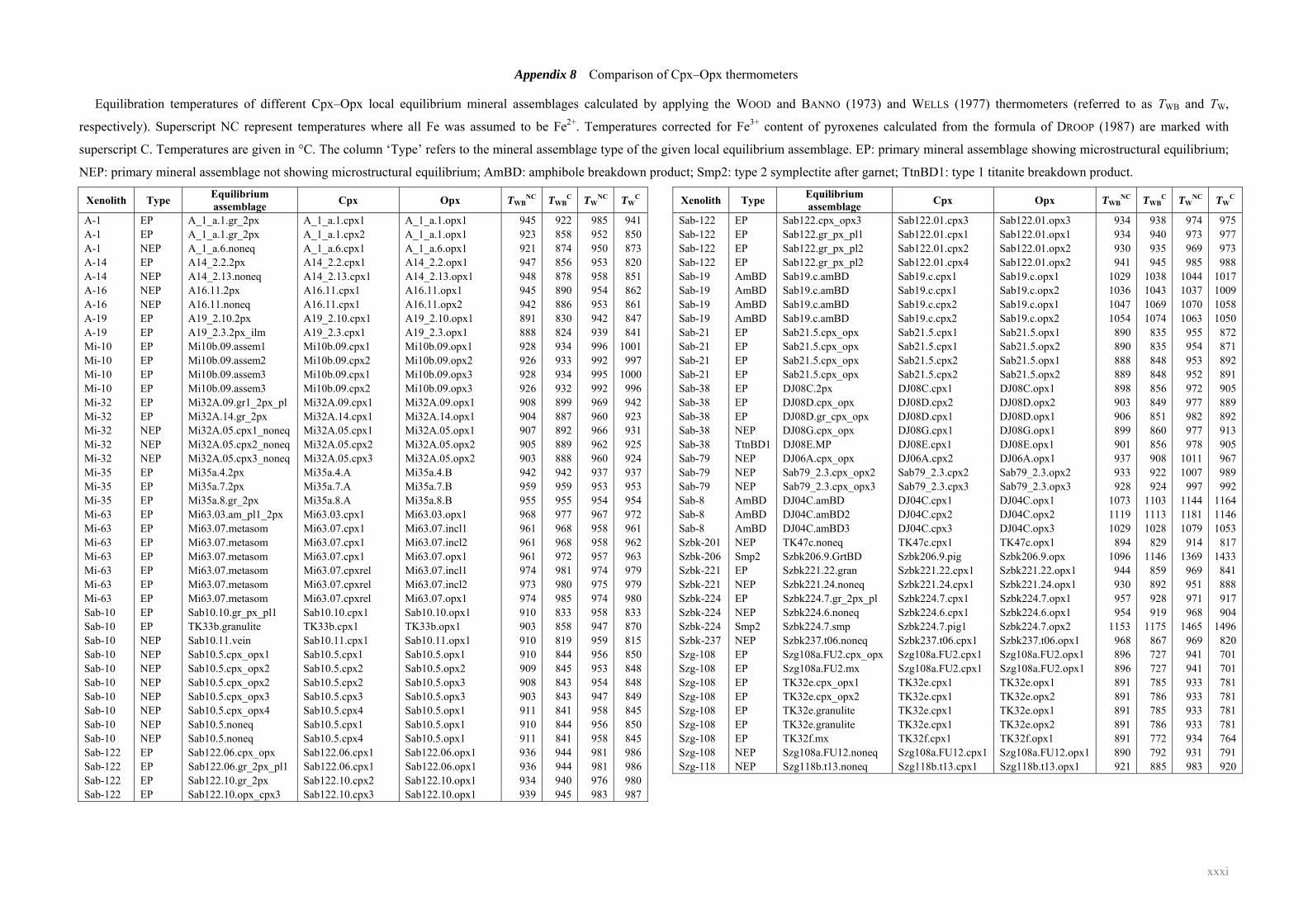
xxxi
Appendix 8 Comparison of Cpx–Opx thermometers
Equilibration temperatures of different Cpx–Opx local equilibrium mineral assemblages calculated by applying the WOOD and BANNO (1973) and WELLS (1977) thermometers (referred to as TWB and TW,
respectively). Superscript NC represent temperatures where all Fe was assumed to be Fe2+. Temperatures corrected for Fe3+ content of pyroxenes calculated from the formula of DROOP (1987) are marked with
superscript C. Temperatures are given in °C. The column ‘Type’ refers to the mineral assemblage type of the given local equilibrium assemblage. EP: primary mineral assemblage showing microstructural equilibrium;
NEP: primary mineral assemblage not showing microstructural equilibrium; AmBD: amphibole breakdown product; Smp2: type 2 symplectite after garnet; TtnBD1: type 1 titanite breakdown product.
Xenolith Type Equilibrium assemblage Cpx Opx TWB
NC TWBC TW
NC TWC
A-1 EP A_1_a.1.gr_2px A_1_a.1.cpx1 A_1_a.1.opx1 945 922 985 941 A-1 EP A_1_a.1.gr_2px A_1_a.1.cpx2 A_1_a.1.opx1 923 858 952 850 A-1 NEP A_1_a.6.noneq A_1_a.6.cpx1 A_1_a.6.opx1 921 874 950 873 A-14 EP A14_2.2.2px A14_2.2.cpx1 A14_2.2.opx1 947 856 953 820 A-14 NEP A14_2.13.noneq A14_2.13.cpx1 A14_2.13.opx1 948 878 958 851 A-16 NEP A16.11.2px A16.11.cpx1 A16.11.opx1 945 890 954 862 A-16 NEP A16.11.noneq A16.11.cpx1 A16.11.opx2 942 886 953 861 A-19 EP A19_2.10.2px A19_2.10.cpx1 A19_2.10.opx1 891 830 942 847 A-19 EP A19_2.3.2px_ilm A19_2.3.cpx1 A19_2.3.opx1 888 824 939 841 Mi-10 EP Mi10b.09.assem1 Mi10b.09.cpx1 Mi10b.09.opx1 928 934 996 1001 Mi-10 EP Mi10b.09.assem2 Mi10b.09.cpx2 Mi10b.09.opx2 926 933 992 997 Mi-10 EP Mi10b.09.assem3 Mi10b.09.cpx1 Mi10b.09.opx3 928 934 995 1000 Mi-10 EP Mi10b.09.assem3 Mi10b.09.cpx2 Mi10b.09.opx3 926 932 992 996 Mi-32 EP Mi32A.09.gr1_2px_pl Mi32A.09.cpx1 Mi32A.09.opx1 908 899 969 942 Mi-32 EP Mi32A.14.gr_2px Mi32A.14.cpx1 Mi32A.14.opx1 904 887 960 923 Mi-32 NEP Mi32A.05.cpx1_noneq Mi32A.05.cpx1 Mi32A.05.opx1 907 892 966 931 Mi-32 NEP Mi32A.05.cpx2_noneq Mi32A.05.cpx2 Mi32A.05.opx2 905 889 962 925 Mi-32 NEP Mi32A.05.cpx3_noneq Mi32A.05.cpx3 Mi32A.05.opx2 903 888 960 924 Mi-35 EP Mi35a.4.2px Mi35a.4.A Mi35a.4.B 942 942 937 937 Mi-35 EP Mi35a.7.2px Mi35a.7.A Mi35a.7.B 959 959 953 953 Mi-35 EP Mi35a.8.gr_2px Mi35a.8.A Mi35a.8.B 955 955 954 954 Mi-63 EP Mi63.03.am_pl1_2px Mi63.03.cpx1 Mi63.03.opx1 968 977 967 972 Mi-63 EP Mi63.07.metasom Mi63.07.cpx1 Mi63.07.incl1 961 968 958 961 Mi-63 EP Mi63.07.metasom Mi63.07.cpx1 Mi63.07.incl2 961 968 958 962 Mi-63 EP Mi63.07.metasom Mi63.07.cpx1 Mi63.07.opx1 961 972 957 963 Mi-63 EP Mi63.07.metasom Mi63.07.cpxrel Mi63.07.incl1 974 981 974 979 Mi-63 EP Mi63.07.metasom Mi63.07.cpxrel Mi63.07.incl2 973 980 975 979 Mi-63 EP Mi63.07.metasom Mi63.07.cpxrel Mi63.07.opx1 974 985 974 980 Sab-10 EP Sab10.10.gr_px_pl1 Sab10.10.cpx1 Sab10.10.opx1 910 833 958 833 Sab-10 EP TK33b.granulite TK33b.cpx1 TK33b.opx1 903 858 947 870 Sab-10 NEP Sab10.11.vein Sab10.11.cpx1 Sab10.11.opx1 910 819 959 815 Sab-10 NEP Sab10.5.cpx_opx1 Sab10.5.cpx1 Sab10.5.opx1 910 844 956 850 Sab-10 NEP Sab10.5.cpx_opx2 Sab10.5.cpx2 Sab10.5.opx2 909 845 953 848 Sab-10 NEP Sab10.5.cpx_opx2 Sab10.5.cpx2 Sab10.5.opx3 908 843 954 848 Sab-10 NEP Sab10.5.cpx_opx3 Sab10.5.cpx3 Sab10.5.opx3 903 843 947 849 Sab-10 NEP Sab10.5.cpx_opx4 Sab10.5.cpx4 Sab10.5.opx1 911 841 958 845 Sab-10 NEP Sab10.5.noneq Sab10.5.cpx1 Sab10.5.opx1 910 844 956 850 Sab-10 NEP Sab10.5.noneq Sab10.5.cpx4 Sab10.5.opx1 911 841 958 845 Sab-122 EP Sab122.06.cpx_opx Sab122.06.cpx1 Sab122.06.opx1 936 944 981 986 Sab-122 EP Sab122.06.gr_2px_pl1 Sab122.06.cpx1 Sab122.06.opx1 936 944 981 986 Sab-122 EP Sab122.10.gr_2px Sab122.10.cpx2 Sab122.10.opx1 934 940 976 980 Sab-122 EP Sab122.10.opx_cpx3 Sab122.10.cpx3 Sab122.10.opx1 939 945 983 987
Xenolith Type Equilibrium assemblage Cpx Opx TWB
NC TWBC TW
NC TWC
Sab-122 EP Sab122.cpx_opx3 Sab122.01.cpx3 Sab122.01.opx3 934 938 974 975 Sab-122 EP Sab122.gr_px_pl1 Sab122.01.cpx1 Sab122.01.opx1 934 940 973 977 Sab-122 EP Sab122.gr_px_pl2 Sab122.01.cpx2 Sab122.01.opx2 930 935 969 973 Sab-122 EP Sab122.gr_px_pl2 Sab122.01.cpx4 Sab122.01.opx2 941 945 985 988 Sab-19 AmBD Sab19.c.amBD Sab19.c.cpx1 Sab19.c.opx1 1029 1038 1044 1017 Sab-19 AmBD Sab19.c.amBD Sab19.c.cpx1 Sab19.c.opx2 1036 1043 1037 1009 Sab-19 AmBD Sab19.c.amBD Sab19.c.cpx2 Sab19.c.opx1 1047 1069 1070 1058 Sab-19 AmBD Sab19.c.amBD Sab19.c.cpx2 Sab19.c.opx2 1054 1074 1063 1050 Sab-21 EP Sab21.5.cpx_opx Sab21.5.cpx1 Sab21.5.opx1 890 835 955 872 Sab-21 EP Sab21.5.cpx_opx Sab21.5.cpx1 Sab21.5.opx2 890 835 954 871 Sab-21 EP Sab21.5.cpx_opx Sab21.5.cpx2 Sab21.5.opx1 888 848 953 892 Sab-21 EP Sab21.5.cpx_opx Sab21.5.cpx2 Sab21.5.opx2 889 848 952 891 Sab-38 EP DJ08C.2px DJ08C.cpx1 DJ08C.opx1 898 856 972 905 Sab-38 EP DJ08D.cpx_opx DJ08D.cpx2 DJ08D.opx2 903 849 977 889 Sab-38 EP DJ08D.gr_cpx_opx DJ08D.cpx1 DJ08D.opx1 906 851 982 892 Sab-38 NEP DJ08G.cpx_opx DJ08G.cpx1 DJ08G.opx1 899 860 977 913 Sab-38 TtnBD1 DJ08E.MP DJ08E.cpx1 DJ08E.opx1 901 856 978 905 Sab-79 NEP DJ06A.cpx_opx DJ06A.cpx2 DJ06A.opx1 937 908 1011 967 Sab-79 NEP Sab79_2.3.cpx_opx2 Sab79_2.3.cpx2 Sab79_2.3.opx2 933 922 1007 989 Sab-79 NEP Sab79_2.3.cpx_opx3 Sab79_2.3.cpx3 Sab79_2.3.opx3 928 924 997 992 Sab-8 AmBD DJ04C.amBD DJ04C.cpx1 DJ04C.opx1 1073 1103 1144 1164 Sab-8 AmBD DJ04C.amBD2 DJ04C.cpx2 DJ04C.opx2 1119 1113 1181 1146 Sab-8 AmBD DJ04C.amBD3 DJ04C.cpx3 DJ04C.opx3 1029 1028 1079 1053 Szbk-201 NEP TK47c.noneq TK47c.cpx1 TK47c.opx1 894 829 914 817 Szbk-206 Smp2 Szbk206.9.GrtBD Szbk206.9.pig Szbk206.9.opx 1096 1146 1369 1433 Szbk-221 EP Szbk221.22.gran Szbk221.22.cpx1 Szbk221.22.opx1 944 859 969 841 Szbk-221 NEP Szbk221.24.noneq Szbk221.24.cpx1 Szbk221.24.opx1 930 892 951 888 Szbk-224 EP Szbk224.7.gr_2px_pl Szbk224.7.cpx1 Szbk224.7.opx1 957 928 971 917 Szbk-224 NEP Szbk224.6.noneq Szbk224.6.cpx1 Szbk224.6.opx1 954 919 968 904 Szbk-224 Smp2 Szbk224.7.smp Szbk224.7.pig1 Szbk224.7.opx2 1153 1175 1465 1496 Szbk-237 NEP Szbk237.t06.noneq Szbk237.t06.cpx1 Szbk237.t06.opx1 968 867 969 820 Szg-108 EP Szg108a.FU2.cpx_opx Szg108a.FU2.cpx1 Szg108a.FU2.opx1 896 727 941 701 Szg-108 EP Szg108a.FU2.mx Szg108a.FU2.cpx1 Szg108a.FU2.opx1 896 727 941 701 Szg-108 EP TK32e.cpx_opx1 TK32e.cpx1 TK32e.opx1 891 785 933 781 Szg-108 EP TK32e.cpx_opx2 TK32e.cpx1 TK32e.opx2 891 786 933 781 Szg-108 EP TK32e.granulite TK32e.cpx1 TK32e.opx1 891 785 933 781 Szg-108 EP TK32e.granulite TK32e.cpx1 TK32e.opx2 891 786 933 781 Szg-108 EP TK32f.mx TK32f.cpx1 TK32f.opx1 891 772 934 764 Szg-108 NEP Szg108a.FU12.noneq Szg108a.FU12.cpx1 Szg108a.FU12.opx1 890 792 931 791 Szg-118 NEP Szg118b.t13.noneq Szg118b.t13.cpx1 Szg118b.t13.opx1 921 885 983 920
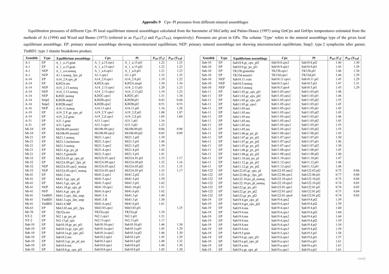
xxxii
Appendix 9 Cpx–Pl pressures from different mineral assemblages
Equilibration pressures of different Cpx–Pl local equilibrium mineral assemblages calculated from the barometer of McCarthy and Patino-Douce (1997) using GrtCpx and GrtOpx temperatures estimated from the
methods of Ai (1994) and Wood and Banno (1973) (referred to as PMP (TA) and PMP (TWB), respectively). Pressures are given in GPa. The column ‘Type’ refers to the mineral assemblage type of the given local
equilibrium assemblage. EP: primary mineral assemblage showing microstructural equilibrium; NEP: primary mineral assemblage not showing microstructural equilibrium; Smp2: type 2 symplectite after garnet;
TtnBD1: type 1 titanite breakdown product.
Xenolith Type Equilibrium assemblage Cpx Pl PMP (TA) PMP (TWB) A-1 EP A_1_a.15.gran A_1_a.15.cpx1 A_1_a.15.pl1 1.22 1.23 A-1 EP A_1_a.15.gran A_1_a.15.cpx1 A_1_a.15.pl2 1.22 1.23 A-1 NEP A_1_a.6.noneq A_1_a.6.cpx1 A_1_a.6.pl1 1.21 1.23 A-1 NEP A1.1.noneq_2px_pl A1.1.cpx1 A1.1.pl1 1.33 1.35 A-14 EP A14_2.8.cpx_pl A14_2.8.cpx1 A14_2.8.pl1 1.19 1.22 A-14 EP KJ02A.mx KJ02A.cpx KJ02A.mxpl 1.30 1.34 A-14 NEP A14_2.13.noneq A14_2.13.cpx1 A14_2.13.pl1 1.20 1.23 A-14 NEP A14_2.13.noneq A14_2.13.cpx1 A14_2.13.pl2 1.19 1.23 A-14 NEP KJ02C.noneq KJ02C.cpx1 KJ02C.pl1 1.31 1.34 A-14 Smp2 KJ02B.smp2 KJ02B.cpx2 KJ02B.pl1 0.43 0.44 A-14 Smp2 KJ02B.smp2 KJ02B.cpx2 KJ02B.pl2 0.51 0.53 A-16 NEP A16.11.noneq A16.11.cpx1 A16.11.pl1 1.16 1.28 A-19 EP A19_2.Y.gr_cpx_pl A19_2.Y.cpx1 A19_2.Z.pl1 1.08 1.07 A-19 EP A19_2.Z.gran A19_2.Z.cpx1 A19_2.Z.pl1 1.05 1.04 A-31 EP A31.1.gran A31.1.cpx1 A31.1.pl1 1.16 A-31 EP A31.3.gran A31.3.cpx1 A31.3.pl1 1.23 Mi-10 EP Mi10b.09.assem1 Mi10b.09.cpx1 Mi10b.09.pl1 0.86 0.90 Mi-10 EP Mi10b.09.assem2 Mi10b.09.cpx2 Mi10b.09.pl2 0.85 0.89 Mi-21 EP Mi21.1.noneq Mi21.1.cpx1 Mi21.1.pl2 1.39 Mi-21 EP Mi21.3.inclusions Mi21.3.cpx1 Mi21.3.pl1 1.44 Mi-21 EP Mi21.3.noneq Mi21.3.cpx2 Mi21.3.pl2 1.39 Mi-21 EP Mi21.4.gr_px_pl Mi21.4.cpx1 Mi21.4.pl1 1.42 Mi-21 EP Mi21.5.granulit Mi21.5.cpx1 Mi21.5.pl1 1.41 Mi-32 EP Mi32A.01.gr_cpx_pl Mi32A.01.cpx2 Mi32A.01.pl1 1.33 1.17 Mi-32 EP Mi32A.09.gr1_2px_pl Mi32A.09.cpx1 Mi32A.09.pl1 1.32 1.16 Mi-32 NEP Mi32A.05.cpx2_noneq Mi32A.05.cpx2 Mi32A.05.pl2 1.31 1.15 Mi-32 NEP Mi32A.05.cpx3_noneq Mi32A.05.cpx3 Mi32A.05.pl1 1.33 1.17 Mi-41 EP Mi41.2.mx Mi41.2.cpx1 Mi41.2.pl2 1.51 Mi-41 EP Mi41.5.gr_cpx_pl Mi41.5.cpx1 Mi41.5.pl1 1.59 Mi-41 EP Mi41.5.gr_cpx_pl Mi41.5.cpx2 Mi41.5.pl1 1.62 Mi-41 NEP Mi41.10.gr_cpx_pl Mi41.10.cpx1 Mi41.10.pl1 1.51 Mi-41 NEP Mi41.6.gr_cpx_pl Mi41.6.cpx1 Mi41.6.pl1 1.62 Mi-41 TtnBD1 Mi41.3.cpx_ilm_smp Mi41.3.A Mi41.3.pl 1.49 Mi-41 TtnBD1 Mi41.3.cpx_ilm_smp Mi41.3.B Mi41.3.pl 1.50 Mi-41 TtnBD1 Mi41.6.MP Mi41.6.cpx2 Mi41.6.pl1 1.61 Mi-63 EP Mi63.03.am_pl1_2px Mi63.03.cpx1 Mi63.03.pl1 1.25 Mi-70 EP TK52a.mx TK52a.cpx TK52a.pl 1.34 NT-2 EP Nt2.1.gr_px_pl Nt2.1.cpx1 Nt2.1.pl1 1.21 NT-2 EP Nt2.13.pl_cpx Nt2.13.cpx1 Nt2.13.pl1 1.17 Sab-10 EP Sab10.10.gr_px_pl1 Sab10.10.cpx1 Sab10.10.pl1 1.46 1.30 Sab-10 EP Sab10.1a.gr_cpx_pl1 Sab10.1a.cpx1 Sab10.1a.pl1 1.45 1.29 Sab-10 EP Sab10.1a.gr_cpx_pl2 Sab10.1a.cpx2 Sab10.1a.pl2 1.46 1.30 Sab-10 EP Sab10.2.mx Sab10.2.cpx1 Sab10.2.pl1 1.45 1.29 Sab-10 EP Sab10.3.gr_px_pl_mx Sab10.3.cpx1 Sab10.3.pl2 1.48 1.32 Sab-10 EP Sab10.6.mx Sab10.6.cpx1 Sab10.6.pl1 1.46 1.30 Sab-10 EP Sab10.8.gr_cpx_pl1 Sab10.8.cpx1 Sab10.8.pl1 1.45 1.30
Xenolith Type Equilibrium assemblage Cpx Pl PMP (TA) PMP (TWB) Sab-10 EP Sab10.8.gr_cpx_pl2 Sab10.8.cpx2 Sab10.8.pl2 1.46 1.30 Sab-10 EP Sab10.9.gr_px_pl1 Sab10.9.cpx1 Sab10.9.pl1 1.45 1.29 Sab-10 EP TK33b.granulite TK33b.cpx1 TK33b.pl1 1.46 1.30 Sab-10 EP TK33d.assem1 TK33d.cpx1 TK33d.pl1 1.44 1.29 Sab-10 NEP Sab10.11.vein Sab10.11.cpx1 Sab10.11.pl1 1.45 1.29 Sab-10 NEP Sab10.5.noneq Sab10.5.cpx1 Sab10.5.pl1 1.47 1.31 Sab-10 NEP Sab10.5.noneq Sab10.5.cpx4 Sab10.5.pl1 1.45 1.29 Sab-11 EP Sab11.03.gr_cpx_pl1 Sab11.03.cpx1 Sab11.03.pl1 1.48 Sab-11 EP Sab11.03.gr_cpx_pl2 Sab11.03.cpx2 Sab11.03.pl1 1.46 Sab-11 EP Sab11.05.gr_cpx_pl1 Sab11.05.cpx3 Sab11.05.pl2 1.55 Sab-11 EP Sab11.05.gr_cpx1 Sab11.05.cpx1 Sab11.05.pl1 1.45 Sab-11 EP Sab11.05.mx Sab11.05.cpx1 Sab11.05.pl1 1.45 Sab-11 EP Sab11.05.mx Sab11.05.cpx1 Sab11.05.pl2 1.45 Sab-11 EP Sab11.05.mx Sab11.05.cpx2 Sab11.05.pl1 1.46 Sab-11 EP Sab11.05.mx Sab11.05.cpx2 Sab11.05.pl2 1.45 Sab-11 EP Sab11.05.mx Sab11.05.cpx3 Sab11.05.pl1 1.55 Sab-11 EP Sab11.05.mx Sab11.05.cpx3 Sab11.05.pl2 1.55 Sab-11 EP Sab11.06.gr_px_pl Sab11.06.cpx1 Sab11.06.pl1 1.45 Sab-11 EP Sab11.07.gr_px_pl1 Sab11.07.cpx1 Sab11.07.pl1 1.50 Sab-11 EP Sab11.07.gr_px_pl2 Sab11.07.cpx2 Sab11.07.pl1 1.46 Sab-11 EP Sab11.07.gr_px_pl3 Sab11.07.cpx1 Sab11.07.pl2 1.50 Sab-11 EP Sab11.08.gr_px_pl1 Sab11.08.cpx1 Sab11.08.pl1 1.45 Sab-11 EP Sab11.08.gr_px_pl2 Sab11.08.cpx2 Sab11.08.pl2 1.46 Sab-11 EP Sab11.10.am_px_pl Sab11.10.cpx1 Sab11.10.pl1 1.47 Sab-11 EP Sab11.12.gr_px_pl1 Sab11.12.cpx1 Sab11.12.pl1 1.46 Sab-11 EP Sab11.12.gr_px_pl2 Sab11.12.cpx2 Sab11.12.pl1 1.48 Sab-122 EP Sab122.03.gr_opx_pl Sab122.03.opx2 Sab122.03.pl2 0.75 0.86 Sab-122 EP Sab122.06.gr_2px_pl1 Sab122.06.cpx1 Sab122.06.pl1 0.77 0.88 Sab-122 EP Sab122.10.px_pl_noneq Sab122.10.cpx3 Sab122.10.pl1 0.75 0.86 Sab-122 EP Sab122.10.px_pl_noneq Sab122.10.cpx3 Sab122.10.pl2 0.74 0.85 Sab-122 EP Sab122.gr_px_pl1 Sab122.01.cpx1 Sab122.01.pl1 0.74 0.85 Sab-122 EP Sab122.gr_px_pl2 Sab122.01.cpx2 Sab122.01.pl2 0.73 0.84 Sab-122 EP Sab122.gr_px_pl2 Sab122.01.cpx4 Sab122.01.pl2 0.74 0.85 Sab-19 EP Sab19.4.grt_cpx_pl Sab19.4.cpx2 Sab19.4.pl2 1.59 Sab-19 EP Sab19.4.grt_cpx_pl2 Sab19.4.cpx3 Sab19.4.pl2 1.59 Sab-19 EP Sab19.4.mx Sab19.4.cpx1 Sab19.4.pl1 1.60 Sab-19 EP Sab19.4.mx Sab19.4.cpx1 Sab19.4.pl2 1.60 Sab-19 EP Sab19.4.mx Sab19.4.cpx2 Sab19.4.pl1 1.60 Sab-19 EP Sab19.4.mx Sab19.4.cpx2 Sab19.4.pl2 1.59 Sab-19 EP Sab19.4.mx Sab19.4.cpx3 Sab19.4.pl1 1.59 Sab-19 EP Sab19.4.mx Sab19.4.cpx3 Sab19.4.pl2 1.59 Sab-19 EP Sab19.5.gran Sab19.5.cpx1 Sab19.5.pl1 1.58 Sab-19 EP Sab19.6.gr_cpx_pl1 Sab19.6.cpx1 Sab19.6.pl1 1.57 Sab-19 EP Sab19.a.grt_cpx_pl Sab19.a.cpx1 Sab19.a.pl1 1.61 Sab-19 EP Sab19.a.mx Sab19.a.cpx1 Sab19.a.pl1 1.61 Sab-19 EP Sab19.e.gr_cpx_pl Sab19.e.cpx1 Sab19.e.pl1 1.61
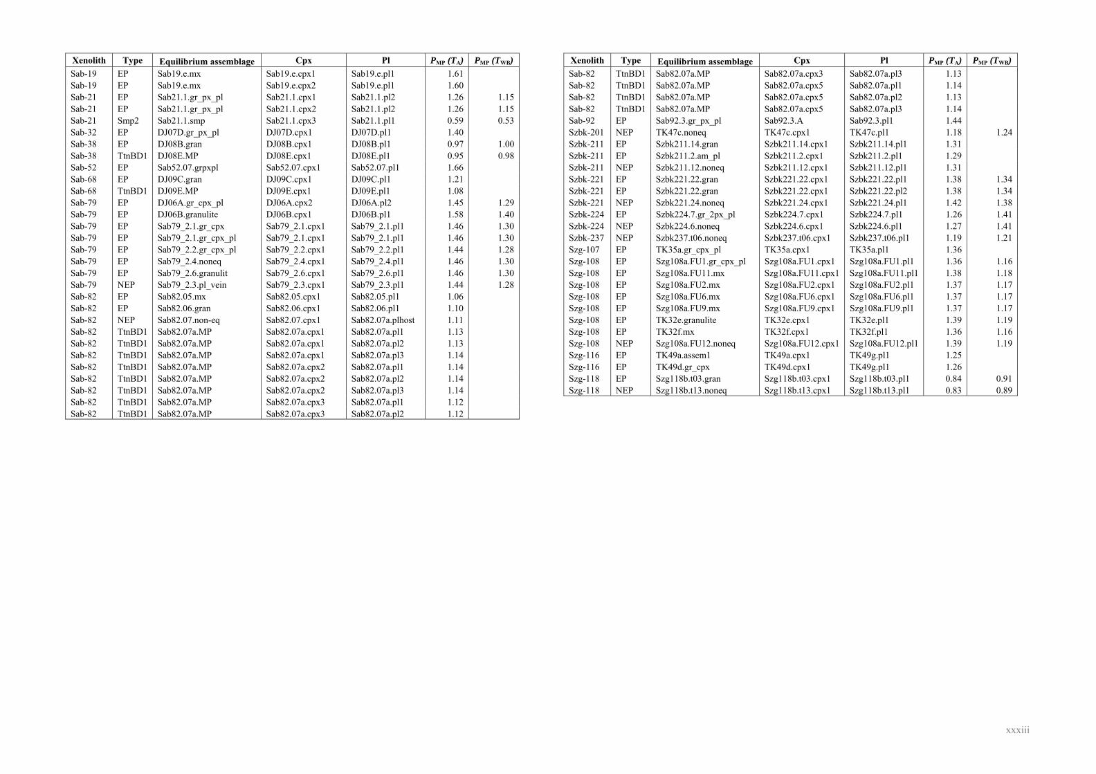
xxxiii
Xenolith Type Equilibrium assemblage Cpx Pl PMP (TA) PMP (TWB) Sab-19 EP Sab19.e.mx Sab19.e.cpx1 Sab19.e.pl1 1.61 Sab-19 EP Sab19.e.mx Sab19.e.cpx2 Sab19.e.pl1 1.60 Sab-21 EP Sab21.1.gr_px_pl Sab21.1.cpx1 Sab21.1.pl2 1.26 1.15 Sab-21 EP Sab21.1.gr_px_pl Sab21.1.cpx2 Sab21.1.pl2 1.26 1.15 Sab-21 Smp2 Sab21.1.smp Sab21.1.cpx3 Sab21.1.pl1 0.59 0.53 Sab-32 EP DJ07D.gr_px_pl DJ07D.cpx1 DJ07D.pl1 1.40 Sab-38 EP DJ08B.gran DJ08B.cpx1 DJ08B.pl1 0.97 1.00 Sab-38 TtnBD1 DJ08E.MP DJ08E.cpx1 DJ08E.pl1 0.95 0.98 Sab-52 EP Sab52.07.grpxpl Sab52.07.cpx1 Sab52.07.pl1 1.66 Sab-68 EP DJ09C.gran DJ09C.cpx1 DJ09C.pl1 1.21 Sab-68 TtnBD1 DJ09E.MP DJ09E.cpx1 DJ09E.pl1 1.08 Sab-79 EP DJ06A.gr_cpx_pl DJ06A.cpx2 DJ06A.pl2 1.45 1.29 Sab-79 EP DJ06B.granulite DJ06B.cpx1 DJ06B.pl1 1.58 1.40 Sab-79 EP Sab79_2.1.gr_cpx Sab79_2.1.cpx1 Sab79_2.1.pl1 1.46 1.30 Sab-79 EP Sab79_2.1.gr_cpx_pl Sab79_2.1.cpx1 Sab79_2.1.pl1 1.46 1.30 Sab-79 EP Sab79_2.2.gr_cpx_pl Sab79_2.2.cpx1 Sab79_2.2.pl1 1.44 1.28 Sab-79 EP Sab79_2.4.noneq Sab79_2.4.cpx1 Sab79_2.4.pl1 1.46 1.30 Sab-79 EP Sab79_2.6.granulit Sab79_2.6.cpx1 Sab79_2.6.pl1 1.46 1.30 Sab-79 NEP Sab79_2.3.pl_vein Sab79_2.3.cpx1 Sab79_2.3.pl1 1.44 1.28 Sab-82 EP Sab82.05.mx Sab82.05.cpx1 Sab82.05.pl1 1.06 Sab-82 EP Sab82.06.gran Sab82.06.cpx1 Sab82.06.pl1 1.10 Sab-82 NEP Sab82.07.non-eq Sab82.07.cpx1 Sab82.07a.plhost 1.11 Sab-82 TtnBD1 Sab82.07a.MP Sab82.07a.cpx1 Sab82.07a.pl1 1.13 Sab-82 TtnBD1 Sab82.07a.MP Sab82.07a.cpx1 Sab82.07a.pl2 1.13 Sab-82 TtnBD1 Sab82.07a.MP Sab82.07a.cpx1 Sab82.07a.pl3 1.14 Sab-82 TtnBD1 Sab82.07a.MP Sab82.07a.cpx2 Sab82.07a.pl1 1.14 Sab-82 TtnBD1 Sab82.07a.MP Sab82.07a.cpx2 Sab82.07a.pl2 1.14 Sab-82 TtnBD1 Sab82.07a.MP Sab82.07a.cpx2 Sab82.07a.pl3 1.14 Sab-82 TtnBD1 Sab82.07a.MP Sab82.07a.cpx3 Sab82.07a.pl1 1.12 Sab-82 TtnBD1 Sab82.07a.MP Sab82.07a.cpx3 Sab82.07a.pl2 1.12
Xenolith Type Equilibrium assemblage Cpx Pl PMP (TA) PMP (TWB) Sab-82 TtnBD1 Sab82.07a.MP Sab82.07a.cpx3 Sab82.07a.pl3 1.13 Sab-82 TtnBD1 Sab82.07a.MP Sab82.07a.cpx5 Sab82.07a.pl1 1.14 Sab-82 TtnBD1 Sab82.07a.MP Sab82.07a.cpx5 Sab82.07a.pl2 1.13 Sab-82 TtnBD1 Sab82.07a.MP Sab82.07a.cpx5 Sab82.07a.pl3 1.14 Sab-92 EP Sab92.3.gr_px_pl Sab92.3.A Sab92.3.pl1 1.44 Szbk-201 NEP TK47c.noneq TK47c.cpx1 TK47c.pl1 1.18 1.24 Szbk-211 EP Szbk211.14.gran Szbk211.14.cpx1 Szbk211.14.pl1 1.31 Szbk-211 EP Szbk211.2.am_pl Szbk211.2.cpx1 Szbk211.2.pl1 1.29 Szbk-211 NEP Szbk211.12.noneq Szbk211.12.cpx1 Szbk211.12.pl1 1.31 Szbk-221 EP Szbk221.22.gran Szbk221.22.cpx1 Szbk221.22.pl1 1.38 1.34 Szbk-221 EP Szbk221.22.gran Szbk221.22.cpx1 Szbk221.22.pl2 1.38 1.34 Szbk-221 NEP Szbk221.24.noneq Szbk221.24.cpx1 Szbk221.24.pl1 1.42 1.38 Szbk-224 EP Szbk224.7.gr_2px_pl Szbk224.7.cpx1 Szbk224.7.pl1 1.26 1.41 Szbk-224 NEP Szbk224.6.noneq Szbk224.6.cpx1 Szbk224.6.pl1 1.27 1.41 Szbk-237 NEP Szbk237.t06.noneq Szbk237.t06.cpx1 Szbk237.t06.pl1 1.19 1.21 Szg-107 EP TK35a.gr_cpx_pl TK35a.cpx1 TK35a.pl1 1.36 Szg-108 EP Szg108a.FU1.gr_cpx_pl Szg108a.FU1.cpx1 Szg108a.FU1.pl1 1.36 1.16 Szg-108 EP Szg108a.FU11.mx Szg108a.FU11.cpx1 Szg108a.FU11.pl1 1.38 1.18 Szg-108 EP Szg108a.FU2.mx Szg108a.FU2.cpx1 Szg108a.FU2.pl1 1.37 1.17 Szg-108 EP Szg108a.FU6.mx Szg108a.FU6.cpx1 Szg108a.FU6.pl1 1.37 1.17 Szg-108 EP Szg108a.FU9.mx Szg108a.FU9.cpx1 Szg108a.FU9.pl1 1.37 1.17 Szg-108 EP TK32e.granulite TK32e.cpx1 TK32e.pl1 1.39 1.19 Szg-108 EP TK32f.mx TK32f.cpx1 TK32f.pl1 1.36 1.16 Szg-108 NEP Szg108a.FU12.noneq Szg108a.FU12.cpx1 Szg108a.FU12.pl1 1.39 1.19 Szg-116 EP TK49a.assem1 TK49a.cpx1 TK49g.pl1 1.25 Szg-116 EP TK49d.gr_cpx TK49d.cpx1 TK49g.pl1 1.26 Szg-118 EP Szg118b.t03.gran Szg118b.t03.cpx1 Szg118b.t03.pl1 0.84 0.91 Szg-118 NEP Szg118b.t13.noneq Szg118b.t13.cpx1 Szg118b.t13.pl1 0.83 0.89
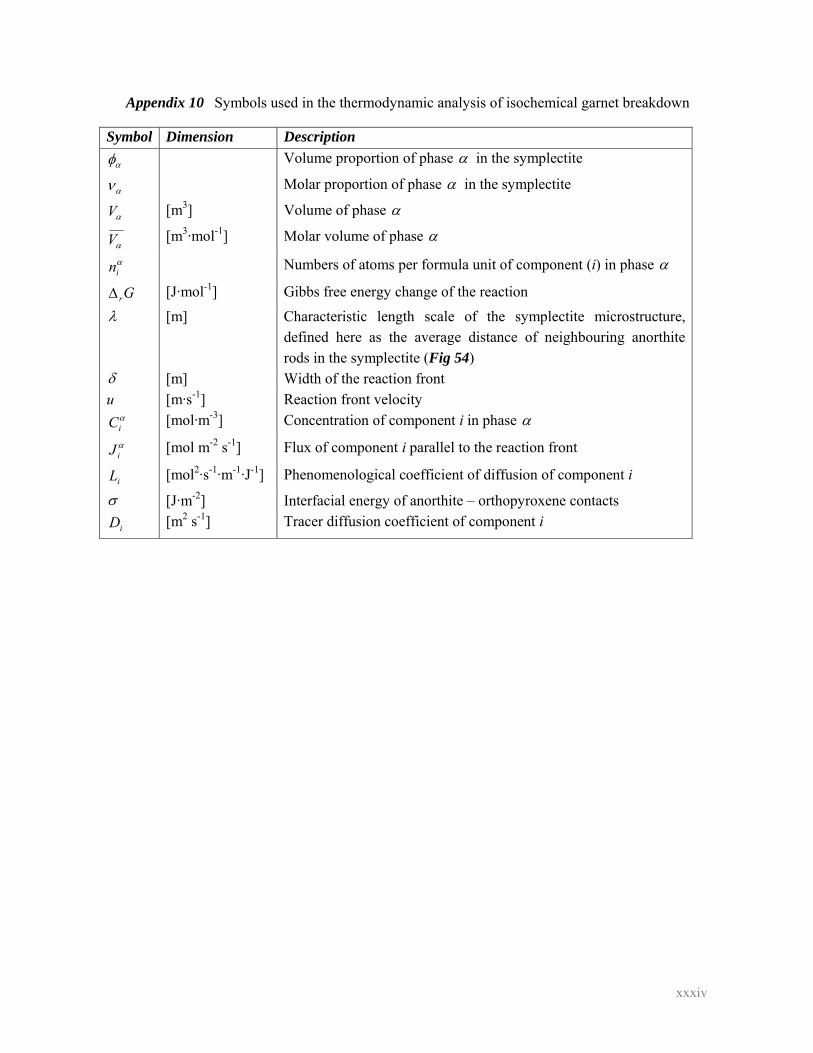
xxxiv
Appendix 10 Symbols used in the thermodynamic analysis of isochemical garnet breakdown
Symbol Dimension Description
αφ Volume proportion of phase α in the symplectite
αν Molar proportion of phase α in the symplectite
αV [m3] Volume of phase α
αV [m3·mol-1] Molar volume of phase α αin Numbers of atoms per formula unit of component (i) in phase α
GrΔ [J·mol-1] Gibbs free energy change of the reaction λ [m] Characteristic length scale of the symplectite microstructure,
defined here as the average distance of neighbouring anorthite rods in the symplectite (Fig 54)
δ [m] Width of the reaction front u [m·s-1] Reaction front velocity
αiC [mol·m-3] Concentration of component i in phase α αiJ [mol m-2 s-1] Flux of component i parallel to the reaction front
iL [mol2·s-1·m-1·J-1] Phenomenological coefficient of diffusion of component i
σ [J·m-2] Interfacial energy of anorthite – orthopyroxene contacts
iD [m2 s-1] Tracer diffusion coefficient of component i