Journal of Modern Applied StatisticalMethods

Volume 16 | Issue 2 Article 30

December 2017

JMASM 49: A Compilation of Some PopularGoodness of Fit Tests for Normal Distribution:Their Algorithms and MATLAB Codes(MATLAB)Metin ÖnerManisa Celal Bayar University, Manisa, Turkey, metin.oner@cbu.edu.tr

İpek Deveci KocakoçDokuz Eylul University, İzmir, Turkey, ipek.deveci@deu.edu.tr

Follow this and additional works at: http://digitalcommons.wayne.edu/jmasm

Part of the Applied Statistics Commons, Social and Behavioral Sciences Commons, and theStatistical Theory Commons

This Algorithms and Code is brought to you for free and open access by the Open Access Journals at DigitalCommons@WayneState. It has beenaccepted for inclusion in Journal of Modern Applied Statistical Methods by an authorized editor of DigitalCommons@WayneState.

Recommended CitationÖner, M., & Kocakoc, I. D. (2017). JMASM 49: A Compilation of Some Popular Goodness of Fit Tests for Normal Distribution: TheirAlgorithms and MATLAB Codes (MATLAB). Journal of Modern Applied Statistical Methods, 16(2), 547-575. doi: 10.22237/jmasm/1509496200

Journal of Modern Applied Statistical Methods

November 2017, Vol. 16, No. 2, 547-575. doi: 10.22237/jmasm/1509496200

Copyright © 2017 JMASM, Inc.

ISSN 1538 − 9472

Metin Öner is an Associate Professor in the School of Applied Sciences. Email him at: metin.oner@cbu.edu.tr.

547

JMASM 49: A Compilation of Some Popular Goodness of Fit Tests for Normal Distribution: Their Algorithms and MATLAB Codes (MATLAB)

Metin Öner Manisa Celal Bayar University

Manisa, Turkey

İpek Deveci Kocakoç Dokuz Eylul University

İzmir, Turkey

The main purpose of this study is to review calculation algorithms for some of the most common non-parametric and omnibus tests for normality, and to provide them as a compiled MATLAB function. All tests are coded to provide p-values for those normality tests, and the proposed function gives the results as an output table.

Keywords: Normality test, non-parametric test, MATLAB function, p-value

Introduction

One of the most important assumptions for parametric statistical methods is that the

sample data come from a normally-distributed population. As this assumption holds,

t-tests, variance analysis, factor analysis, and many more methods gain power.

Normality of error terms is one of the most important assumptions for regression

analysis. For many statistical analyses, a normality test is one of the most important

and necessary things to do along with the examination of distributional features of

data with descriptive statistics, outlier detection, and heteroscedasticity tests.

Hypotheses for fitness testing if sample data or variable(s) follow a normal

distribution (i.e. goodness-of-fit testing) are as follows:

H0: x ∈ N(μ, σ)

H1: x ∉ N(μ, σ)

Most popular normality tests can be listed as follows:

SOME POPULAR GOODNESS OF FIT TESTS FOR NORMALITY

548

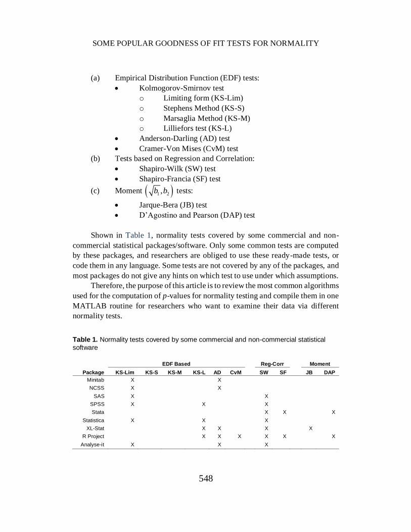
(a) Empirical Distribution Function (EDF) tests:

Kolmogorov-Smirnov test

o Limiting form (KS-Lim)

o Stephens Method (KS-S)

o Marsaglia Method (KS-M)

o Lilliefors test (KS-L)

Anderson-Darling (AD) test

Cramer-Von Mises (CvM) test

(b) Tests based on Regression and Correlation:

Shapiro-Wilk (SW) test

Shapiro-Francia (SF) test

(c) Moment 1 2,b b tests:

Jarque-Bera (JB) test

D’Agostino and Pearson (DAP) test

Shown in Table 1, normality tests covered by some commercial and non-

commercial statistical packages/software. Only some common tests are computed

by these packages, and researchers are obliged to use these ready-made tests, or

code them in any language. Some tests are not covered by any of the packages, and

most packages do not give any hints on which test to use under which assumptions.

Therefore, the purpose of this article is to review the most common algorithms

used for the computation of p-values for normality testing and compile them in one

MATLAB routine for researchers who want to examine their data via different

normality tests. Table 1. Normality tests covered by some commercial and non-commercial statistical

software

EDF Based Reg-Corr Moment

Package KS-Lim KS-S KS-M KS-L AD CvM SW SF JB DAP

Minitab X X

NCSS X X

SAS X X

SPSS X X X

Stata X X X

Statistica X X X

XL-Stat X X X X

R Project X X X X X X

Analyse-it X X X

ÖNER & DEVECI KOCAKOÇ

549

Empirical Distribution Function Tests

Let y1, y2,…, yn be ordered values of x1, x2,…, xn sample values. If i denotes the

frequency of yk in kth order, the empirical distribution function is defined as the

following step function:

1

1

0,

F , , 1,2, 1

1,

n k k

n

y y

y i n y y y k n

y y

(1)

The following EDF tests are based on this function. Computation procedures are

given here for these tests. For further information about the formulas and the

interpretation of EDF statistics, see Hollander and Wolfe (1999) and Gibbons and

Chakraborti (1992). For details about the k-sample analogs of the Kolmogorov-

Smirnov and Cramer-von Mises statistics used by NPAR1WAY, see Kiefer (1959).

Kolmogorov-Smirnov Normality Test

The Kolmogorov-Smirnov (KS) test statistic is computed with the help of the Dn

statistic, which is defined as follows:

0sup F Fn nx

D x x (2)

where “sup” in equation (2) denotes the supremum, that is the maximum of the

values in a given interval.

The Dn test statistic will be the greatest vertical distance between F(x) and

F0(x) (Kolmogorov, 1933):

max ,n n nD D D (3)

where 1 0F Fn k kD x x

and 0F Fn k kD x x . The KSz statistic is

computed as follows:

KS nz nD (4)

SOME POPULAR GOODNESS OF FIT TESTS FOR NORMALITY

550

The stepwise procedure given below covers the mutual steps required for

calculation of p-values for four KS-type tests. The first eight steps are also identical

for the AD and CvM tests. The rest of the calculation steps are given for each EDF

test.

Step 1: Enter sample x vector

Step 2: yi = sort(x)

Step 3: i = 1, 2,…, n

Step 4: Fn(y) = i / n

Step 5: mean(y) = Σ yi / n

Step 6: 2

σ mean 1iy n y y

Step 7: zi = (yi – mean(y)) / σ(y)

Step 8: F0(y) = ui = ϕ(zi)

Step 9: Dplus = abs(F0(y) – i / n)

Step 10: Dminus = abs(F0(y) – (i – 1) / n)

Step 11: Dn = max(Dplus, Dminus)

Step 12: KS nz nD

Limiting Form

Most statistical packages use this method to calculate the KSz test statistic. In this

method, if n → ∞ the distribution of the KSz statistic nnD is asymptotically

Kolmogorov distributed. This statistic has the following formula (Facchinetti,

2009):

2 21 2

1

lim Pr 1 2 1 ek k x

nn

k

nD x

(5)

This method is suitable for cases where the sample size is large and the distribution

parameters are known. However, it is being used in cases where n is small and

parameters are not known. The p-value for this test can be calculated by the

following step:

20 2

2

20

Step 13: -value 1 1 exp 2k

n

k

p k nD

ÖNER & DEVECI KOCAKOÇ

551

Marsaglia Method

This method was introduced by Marsaglia, Tsang, and Wang (2003). Pr nD d

is calculated by this formula:

!

Pr n kkn

nD d t

n (6)

Here, tkk is the (k, k)th element of the matrix Hn, H is an m × m matrix, m = 2k – 1,

d = (k – h) / n, with k (a positive integer), and 0 ≤ h < 1.

Although this method has a complicated algorithm, it provides 13-15 digit

accuracy for n ranging from 2 to at least 16000 for one-tailed p-value calculation.

Step 13: Calculate k, m, and h values:

k = Round up (nDn)

m = 2k – 1

h = k – nDn

Step 14: Get the H matrix using the following procedure:

Get the first column of the H matrix except the element

Hmatrix (m, 1).

Loop i = 1: m – 1

Hmatrix (i, 1) = (1 – hi) / i!

End

Get the mth row of the H matrix except the element Hmatrix (m, 1).

Hmatrix (m, c) = Hmatrix (r, 1)T, r = 1,…, m – 1, and c = m – r + 1

Get the other elements of the H matrix.

Loop i = 1: m – 1

Loop j = 2: m

If i – j + 1 ≥ 0

Hmatrix (i, j) = 1 / (i – j + 1)!

Else

Hmatrix (i, j) = 0

End

End

End

Get the element Hmatrix (m, 1).

If h ≤ 0.5

SOME POPULAR GOODNESS OF FIT TESTS FOR NORMALITY

552

Hmatrix (m, 1) = (1 – 2hm) / m!

Else

Hmatrix (m, 1) = (1 – 2hm + max(0, 2h – 1)m) / m!

Step 15: Calculate the p-value

!

-value Pr 1 Pr 1 ,n

n n n

np D d D d k k

n H

Stephens’ Method

Stephens’ method uses a D* test statistic, which is revised by using Dn, to test

normality for cases where parameters are not known. The test statistic D* is

calculated based on n via the following equation:

0.85

0.01nD D nn

(7)

Stephens (1986, p. 123) obtained upper tail critical D* values by Monte Carlo

simulations and tabulated them. Here, the p-value is calculated by linear

interpolation based on the values of Stephens’ table and the calculation steps are as

follows:

Step 13: Calculate the modified D* statistic from equation (7).

Step 14: Calculate the p-value via linear interpolation by using Stephens’

critical value table:

-value

report -value 0.15 0.775

0.15 0.775 0.10 0.15 0.819 0.775 0.775 0.819

0.10 0.819 0.05 0.10 0.895 0.819 0.819 0.895

0.05 0.895 0.025 0.05 0.995 0.895 0.895 0.995

0.025 0.

p

p D

D D

D D

D D

D

995 0.01 0.025 1.035 0.995 0.995 1.035

report -value 0.01 1.035

D

p D

ÖNER & DEVECI KOCAKOÇ

553

Lilliefors Test for Normality

The Lilliefors (LF) test was presented as a correction of the Kolmogorov-Smirnov

test by Lilliefors (1967). Dellal and Wilkinson (1986) provided a numerical

approximation to calculate p-values for this method. The LF test is an extension of

the Kolmogorov-Smirnov test to the case where the parameters of the hypothesized

normal distribution are unknown and estimated by a sample data set. If the mean

and variance parameters of the hypothesized normal distribution are not known, the

LF test or Stephens’ method should be used instead of the Kolmogorov-Smirnov

test. The LF test as a correction of the Kolmogorov-Smirnov test should not be

confused with the original Kolmogorov-Smirnov test. This study adopts the

algorithm used by the statistical software SPSS to calculate the p-value of the LF

test, which is based on the use of the critical value table and formulation of Dellal

and Wilkinson. The algorithm is given below:

Step 13: Find the critical values D20 and D15 corresponding to n from the

table given by Dellal and Wilkinson (1986). This table is included

in the MATLAB codes in the Appendix. D20 and D15 are the

critical values corresponding to α = 0.20 and α = 0.15 for the LF

normality test, respectively. If n lies between two lower and upper n

values, find the critical values D20 and D15 by linear interpolation.

The equations of linear interpolation for the critical values D20 and

D15 are given below:

upper lower

lower lower

upper lower

upper lower

lower lower

upper lower

20 2020 20

15 1515 15

D DD D n n

n n

D DD D n n

n n

Step 14: Find the values of a1, b1, c1, a2, b2, and c2 via the following

equations:

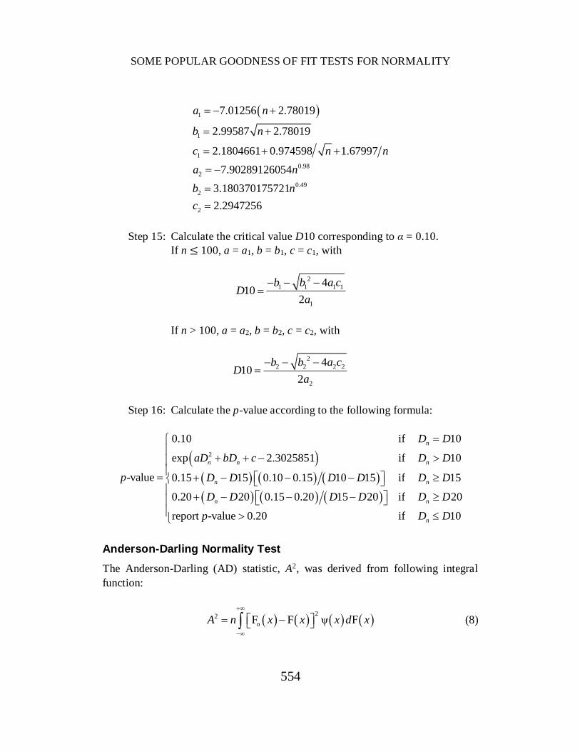
SOME POPULAR GOODNESS OF FIT TESTS FOR NORMALITY

554

1

1

1

0.98

2

0.49

2

2

7.01256 2.78019

2.99587 2.78019

2.1804661 0.974598 1.67997

7.90289126054

3.180370175721

2.2947256

a n

b n

c n n

a n

b n

c

Step 15: Calculate the critical value D10 corresponding to α = 0.10.

If n ≤ 100, a = a1, b = b1, c = c1, with

2

1 1 1 1

1

410

2

b b a cD

a

If n > 100, a = a2, b = b2, c = c2, with

2

2 2 2 2

2

410

2

b b a cD

a

Step 16: Calculate the p-value according to the following formula:

2

0.10 if 10

exp 2.3025851 if 10

-value 0.15 15 0.10 0.15 10 15 if 15

0.20 20 0.15 0.20 15 20 if 20

report -value 0.20 if 10

n

n n n

n n

n n

n

D D

aD bD c D D

p D D D D D D

D D D D D D

p D D

Anderson-Darling Normality Test

The Anderson-Darling (AD) statistic, A2, was derived from following integral

function:

22 F F ψ FnA n x x x d x

(8)

ÖNER & DEVECI KOCAKOÇ

555

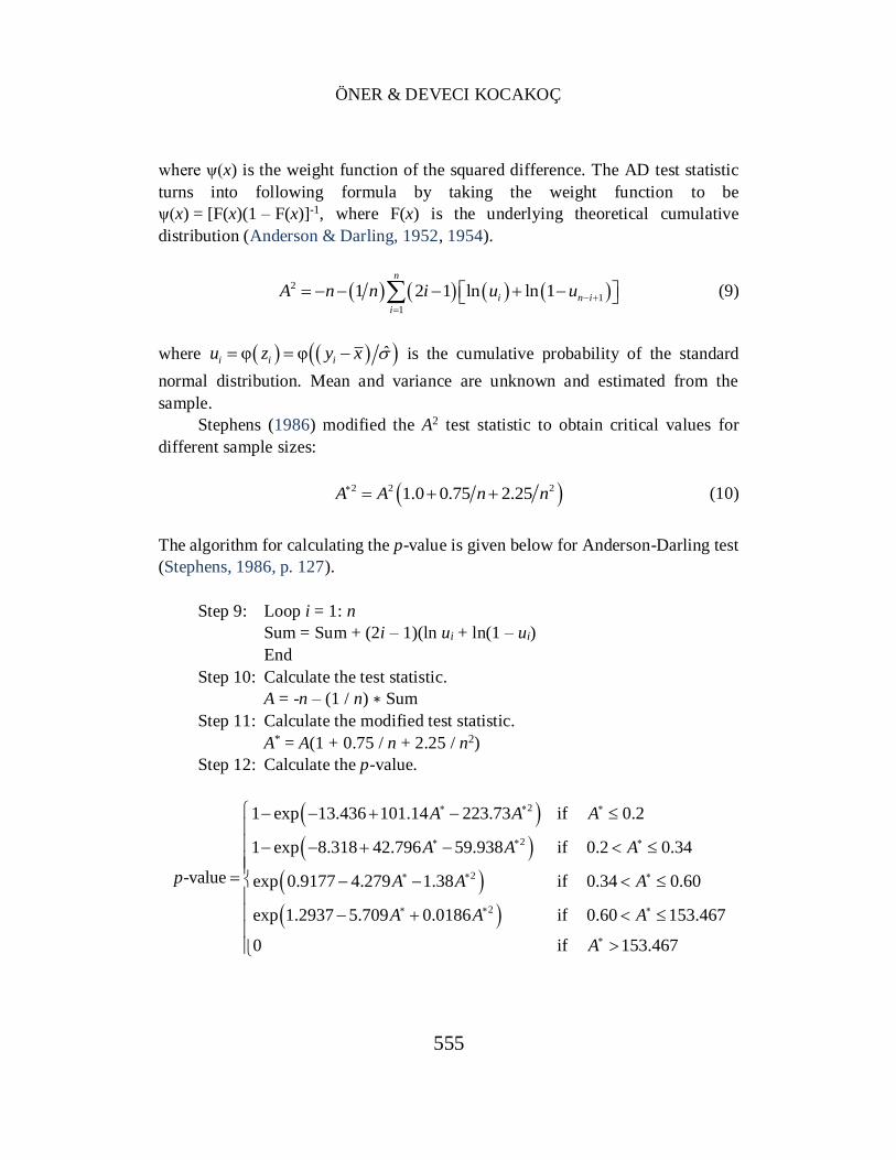
where ψ(x) is the weight function of the squared difference. The AD test statistic

turns into following formula by taking the weight function to be

ψ(x) = [F(x)(1 – F(x)]-1, where F(x) is the underlying theoretical cumulative

distribution (Anderson & Darling, 1952, 1954).

2

1

1

1 2 1 ln ln 1n

i n i

i

A n n i u u

(9)

where ˆφ φi i iu z y x is the cumulative probability of the standard

normal distribution. Mean and variance are unknown and estimated from the

sample.

Stephens (1986) modified the A2 test statistic to obtain critical values for

different sample sizes:

2 2 21.0 0.75 2.25A A n n (10)

The algorithm for calculating the p-value is given below for Anderson-Darling test

(Stephens, 1986, p. 127).

Step 9: Loop i = 1: n

Sum = Sum + (2i – 1)(ln ui + ln(1 – ui)

End

Step 10: Calculate the test statistic.

A = -n – (1 / n) ∗ Sum

Step 11: Calculate the modified test statistic.

A* = A(1 + 0.75 / n + 2.25 / n2)

Step 12: Calculate the p-value.

2

2

2

2

1 exp 13.436 101.14 223.73 if 0.2

1 exp 8.318 42.796 59.938 if 0.2 0.34

-value exp 0.9177 4.279 1.38 if 0.34 0.60

exp 1.2937 5.709 0.0186 if 0.60 153.467

0 if 153.467

A A A

A A A

p A A A

A A A

A

SOME POPULAR GOODNESS OF FIT TESTS FOR NORMALITY

556

Cramer-von Mises Test

Csörgö and Faraway (1996) noted the Cramer-von Mises (CvM) test was

independently presented by Cramer (1928) and von Mises (1931). The CvM test is

derived from the same integral function as the AD statistic:

22 F F ψ FnW n x x x d x

(11)

where ψ(x) is a weight function of squared differences. When ψ(x) = 1, the statistic

is referred to as the CvM statistic W2 and, when ψ(x) = [F(x)(1 – F(x)]-1, the statistic

is referred to as the AD statistic A2.

The CvM test statistic W2 can be written explicitly as

2

2

0

1

1 2 1F

12 2

n

i

i

iW y

n n

(12)

where F0(yi) is the cumulative distribution function of the specified distribution and

the yi are the sorted values of the xi data set (Scott & Stewart, 2011).

Stephens (1986, p.127) provided the calculation procedure for a modified

statistic W*2 = W2(1 + 0.5 / n) as follows:

Step 9: Loop i = 1: n

Sum = Sum + (ui – (2i – 1) / 2n)2

End

Step 10: Calculate the test statistic.

W = (1 / 12n) + Sum

Step 11: Calculate the modified test statistic.

W* = W(1 + 0.5 / n)

Step 12: Calculate the p-value

2

2

2

2

1 exp 13.953 775.5 12542.61 if 0.0275

1 exp 5.903 179.546 1515.29 if 0.0275 0.051-value

exp 0.886 31.62 10.897 if 0.051 0.092

1.111 34.242 12.832 if 0.093

W W W

W W Wp

W W W

W W W

ÖNER & DEVECI KOCAKOÇ

557

Regression and Correlation Based Tests

Shapiro-Wilk Test

Let y1, y2,…, yi,…, yn be ordered values of n independent and identically distributed

random samples (x1, x2,…, xi,…, xn) coming from a population with unknown mean

µ ∈ ℜ and unknown σ > 0. The Shapiro-Wilk statistic W for testing normality is

then defined as

2

1

2

1

n

i ii

n

ii

a yW

y y

(13)

where ai are elements of the vector

1

1/21 1

m Va

m V V m

where m' = (m1, m2,…, mn) is the vector of expected values of normal order

statistics and V = [cov(yi, yj)] is the covariance matrix of order statistics (Shapiro

& Wilk, 1965).

Royston (1982) provided an approximation method for the calculation of the

p-value for a normalized W statistic. This method calculates the p-value of the test

as the upper tail of the standard normal distribution. The algorithm is given below:

Step 1: Sort the sample observations in ascending order, i.e. 1, , nx xx

into 1, , ny yy .

Step 2: Calculate Blom scores m (Solomon & Sawilowsky, 2009).

1 0.375φ

0.25i

im

n

Step 3: T 2

1

n

iim m

m m

Step 4: Calculate the coefficients ai from the following equations:

For i = 1, 2, n – 1, n, and with 1u n :

SOME POPULAR GOODNESS OF FIT TESTS FOR NORMALITY

558

5 4 3 2

5 4 3 2

1

1

2 1

2.70606 4.43469 2.07119 0.14798 0.22116

3.58263 5.68263 1.75246 0.29376 0.04298

n n

n n

n

n

a u u u u u m m

a u u u u u m m

a a

a a

For 3 ≤ i ≤ n – 2:

2 2

1

2 2

1

2 2, where

1 2 2

n ni i

n n

m m ma m

a a

Step 5: Calculate the Shapiro-Wilk test statistic W from equation (13).

Step 6: Normalize the test statistic W:

ln 1 W

Z

where, for x = ln n,

2 3

2

1.5861 0.31082 0.083751 0.0038915

exp 0.4803 0.082676 0.0030302

x x x

x x

Step 7: Calculate the p-value as the upper tail from the standard normal

distribution:

p-value = Pr(Z ≥ z) = 1 – ϕ(|z|)

Shapiro Francia Test

The Shapiro Francia test statistic W' is given by

2 2

1 1

2 2 2

1 1 1

n n

i i i ii i

n n n

i i ii i i

b y m XW

y y y y m

(14)

ÖNER & DEVECI KOCAKOÇ

559

where y1 ≤…≤ yn are ordered statistics, the im are Blom scores, and

T T

1T 2

1

, , , ,i nn

i

b b b

m mb

m m m

which is called the Shapiro Francia statistic for normality tests (Shapiro & Francia,

1972). If the sample data are leptokurtic, the Shapiro-Francia test is recommended;

whereas for platycurtic data, the Shapiro-Wilk test is preferred.

Royston (1993) proposed an approximation for the Shapiro-Francia test to

calculate the p-value. Mbah and Paothong (2015) use Royston’s approximation

algorithm for p-value calculation when they compared the Shapiro-Francia test with

other tests. The algorithm for Royston’s approximation (for sample sizes

5 ≤ n ≤ 5000) is given below:

Step 1: Sort the sample observations in ascending order, i.e. 1, , nx xx

into 1, , ny yy .

Step 2: Calculate the Shapiro Francia test statistic W' from equation (14).

Step 3: Normalize the test statistic W'.

ln 1 W

Z

where, for u = ln(n), v = ln(u),

1.2725 1.0521

1.0308 0.26758 2

v u

v u

Step 4: Calculate the p-value as the upper tail from the standard normal

distribution:

p-value = Pr(Z ≥ z) = 1 – ϕ(|z|)

SOME POPULAR GOODNESS OF FIT TESTS FOR NORMALITY

560

Moment Tests

Jarque-Bera Test

The Jarque-Bera (JB) test is a goodness of fit measure calculated from sample

kurtosis and skewness (Jarque & Bera, 1987). The normal distribution has a

skewness coefficient of zero and a kurtosis of three. The test statistic JB is then

defined by:

22

1 2 3JB

6 24

b bn

(15)

where the sample skewness is 3 2

1 3 2b and the sample kurtosis is

2

2 4 2b , where μ2, μ3, and μ4 are the second, third, and fourth central moments,

respectively. The jth moment is calculated by

1

1, 2,3,4

nj

j i

i

x x jn

(16)

The JB statistic has an asymptotic chi-square distribution with two degrees of

freedom and H0 should be rejected at a significance level α if 2JB 2 .

The algorithm for calculating the JB test statistic is as follows:

Step 1: The sample vector x is entered.

Step 2: mean ix nx .

Step 3: Second moment 2

2 1mean

n

iix n

x .

Step 4: Third moment 3

3 1mean

n

iix n

x .

Step 5: Fourth moment 4

4 1mean

n

iix n

x .

Step 6: Skewness 3 2

1 3 2b .

Step 7: Kurtosis 2

2 4 2b .

Step 8: Calculate the JB test statistic from equation (16).

Step 9: Calculate the p- value from the chi-square distribution with two

degrees of freedom.

ÖNER & DEVECI KOCAKOÇ

561

D’Agostino and Pearson Test

The D’Agostino and Pearson (DAP) test aggregates the skewness and kurtosis tests.

The test statistic is defined by

2 2

1 2DAP Z Zb b (17)

The skewness test statistic 1Z b and kurtosis test statistic 2Z b are

approximately normally distributed, and the DAP test statistic has an asymptotic

chi-square distribution with two degrees of freedom (D’Agostino & Pearson, 1973).

The algorithm for calculating the p-value of DAP test is given below:

Step 1: Compute the sample skewness 3 2

1 3 2b .

Step 2: Compute the following values:

1

2

2 1

1 22

2 1

1 22

1 3

6 2

3 27 70 1 3β

2 5 7 9

1 2β 1

2 1

n nY b

n

n n n nb

n n n n

W b

W

Step 3: Compute the skewness test statistic 1Z b :

1 2

2

1

1Z ln 1

ln

Y Yb

W

Step 4: Compute the sample kurtosis 2

2 4 2b .

Step 5: Compute the following values:

SOME POPULAR GOODNESS OF FIT TESTS FOR NORMALITY

562

2

2 2

2 2

2

1 22

1 2

1 2

1 21 2 1 2

3 1E

1

24 2 3Var

1 3 5

E

Var

6 5 2 6 3 5β

7 9 2 3

8 2 46 1

ββ β

nb

n

n n nb

n n n

b bX

b

n n n nb

n n n n n

Abb b

Step 6: Compute the kurtosis test statistic 2Z b .

1 3

2

1 2 1 2Z 1

92 9 1 2 4

Ab

AA X A

Step 7: Compute the DAP test statistic from equation (17).

2 2

1 2DAP Z Zb b

Step 8: Calculate the p-value from the chi-square distribution with two

degrees of freedom.

Codes, Execution, and Output

All algorithms for these ten normality tests are coded in the Matlab2015

environment and presented as a function (normalitytest.m). Data should be a 1 × n

row vector (in “x = […]” format) and entered as a variable in the workspace. The

function gives a display of results, as well as a 10 × 3 matrix named “Results,”

including test statistics in the first column, p-values in the second, and test result in

the last. The code file is available both as an Appendix and as an .m file in the

MathWorks File Exchange under the name “normality test package” (Öner &

Deveci Kocakoç, 2016).

ÖNER & DEVECI KOCAKOÇ

563

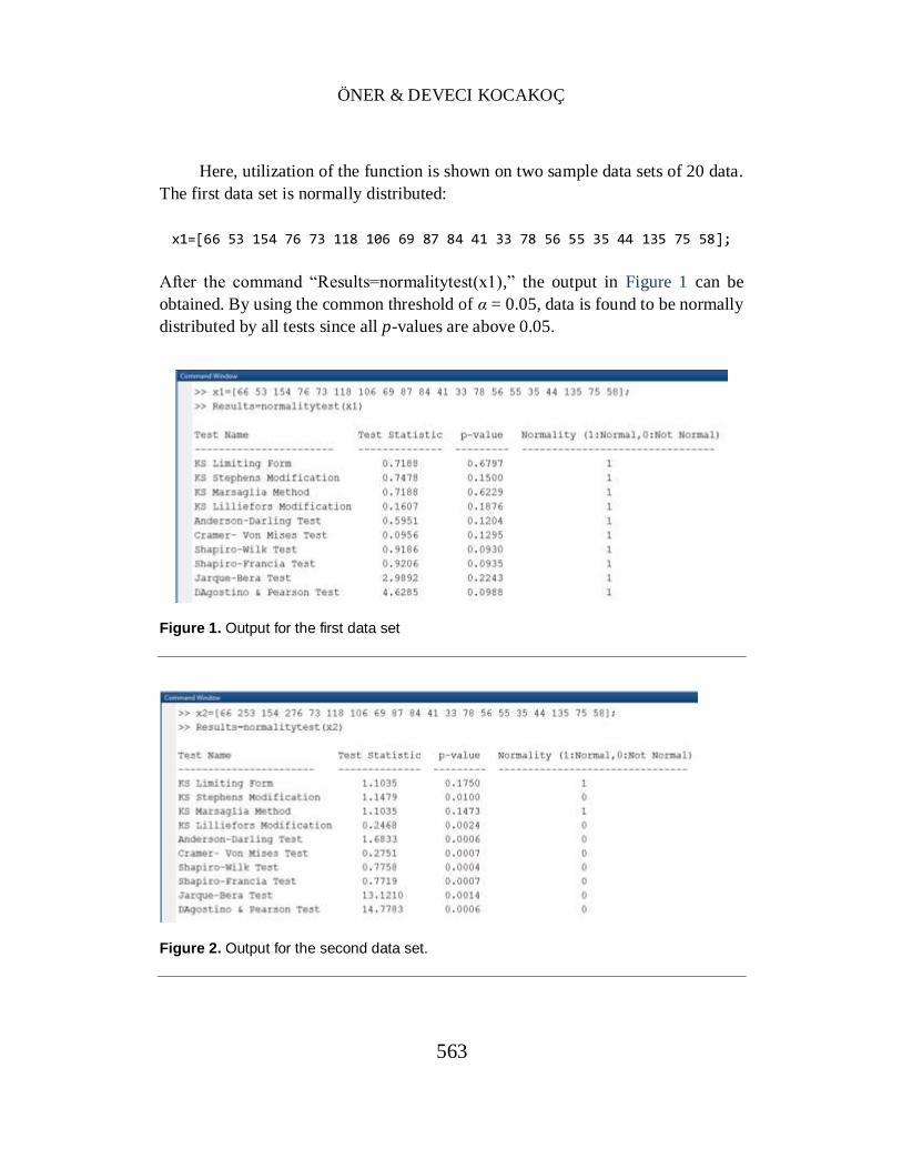
Here, utilization of the function is shown on two sample data sets of 20 data.

The first data set is normally distributed:

x1=[66 53 154 76 73 118 106 69 87 84 41 33 78 56 55 35 44 135 75 58];

After the command “Results=normalitytest(x1),” the output in Figure 1 can be

obtained. By using the common threshold of α = 0.05, data is found to be normally

distributed by all tests since all p-values are above 0.05.

Figure 1. Output for the first data set

Figure 2. Output for the second data set.

SOME POPULAR GOODNESS OF FIT TESTS FOR NORMALITY

564

The second data set is disturbed by changing some of the values in the first

data set:

x2=[66 253 154 276 73 118 106 69 87 84 41 33 78 56 55 35 44 135 75 58];

After the command “Results=normalitytest(x2),” the output in Figure 2 can be

obtained. By using the common threshold of α = 0.05, data is found to be normally

distributed by only two of the tests. The KS test is known to have some problems

with outliers and small sample sizes (Steinskog, Tjøstheim, Kvamstø, 2007). The

Stephens’ and Lilliefors modifications seem to overcome these problems, while the

limiting form and Marsaglia method do not. Since it is not in the scope of this article

to discuss the powers of the tests, the rest of the interpretation is left to the reader.

The function also gives these results as a matrix to use for other purposes. By

this function, a gap in statistical computing can be filled for users of MATLAB as

well as for researchers who would like to know the calculation details of these test

statistics. This MATLAB function can be used to compute all ten test statistics and

to have the results of normality tests with just one command. The next step after

this study is to build an API with a user-friendly interface to perform the tests

without the need of any MATLAB knowledge.

References

Anderson, T. W., & Darling, D. A. (1952). Asymptotic theory of certain

“goodness of fit” criteria based on stochastic processes. The Annals of

Mathematical Statistics, 23(2), 193-212. doi: 10.1214/aoms/1177729437

Anderson, T. W., & Darling, D. A. (1954). A test of goodness of fit. Journal

of the American Statistical Association, 49(268), 765-769. doi:

10.1080/01621459.1954.10501232

Csörgö, S., & Faraway, J. J. (1996).The exact and asymptotic distributions

of Cramer-von Mises statistics. Journal of Royal Statistical Society. Series B

(Methodological), 58(1), 221-234. Available from

http://www.jstor.org/stable/2346175

D’Agostino, R. B., & Pearson, E. S. (1973). Tests for departures from

normality. Empirical results for the distribution of b2 and √b1. Biometrika, 60(3),

613-622. doi: 10.1093/biomet/60.3.613

ÖNER & DEVECI KOCAKOÇ

565

Dellal, G. E., & Wilkinson, L. (1986). An analytic approximation to the

distribution of Lilliefors’s test statistic for normality. The American Statistician,

40(4), 294-296. doi: 10.1080/00031305.1986.10475419

Facchinetti, S. (2009). A procedure to find exact critical values of

Kolmogorov-Smirnov test. Statistica Applicata – Italian Journal of Applied

Statistics, 21(3-4), 337-359. Available from http://sa-ijas.stat.unipd.it/sites/sa-

ijas.stat.unipd.it/files/IJAS_3-4_2009_07_Facchinetti.pdf

Jarque, C. M., & Bera, A. K. (1987). A test for normality of observations

and regression residuals. International Statistical Review, 55(2), 163-172. doi:

10.2307/1403192

Kolmogorov, A. (1933). Sulla determinazione empirica di una leggi di

distribuzione [On the empirical determination of a distribution]. Giornale

dell’Istituto Italiano degli Attuari, 4, 83-91.

Lilliefors, H. W. (1967). On the Kolmogorov-Smirnov test for normality

with mean and variance unknown. Journal of the American Statistical

Association, 62(318), 399-402. doi: 10.1080/01621459.1967.10482916

Marsaglia, G., Tsang, W. W., & Wang, J. (2003). Evaluating Kolmogorov’s

distribution. Journal of Statistical Software, 8(18). doi: 10.18637/jss.v008.i18

Mbah, A. K., & Paothong, A. (2015). Shapiro-Francia test compared to

other normality test using expected p-value. Journal of Statistical Computation

and Simulation, 85(15), 3002-3016. doi: 10.1080/00949655.2014.947986

Öner, M., Deveci Kocakoç, I. (2016). Normality test package [MATLAB

function]. Retrieved from

https://www.mathworks.com/matlabcentral/fileexchange/60147-normality-test-

package

Royston, P. (1982). An extension of Shapiro and Wilk’s W test for normality

to large samples. Journal of the Royal Statistical Society. Series C (Applied

Statistics), 31(2), 115-124. doi: 10.2307/2347973

Royston, P. (1993). A pocket-calculator algorithm for the Shapiro-Francia

test for non-normality: An application to medicine. Statistics in Medicine, 12(2),

181-184. doi: 10.1002/sim.4780120209

Scott, W. F., & Stewart, B. (2011). Tables for the Lilliefors and modified

Cramer-von Mises tests of normality. Communications in Statistics – Theory and

Methods, 40(4), 726-730. doi: 10.1080/03610920903453467

SOME POPULAR GOODNESS OF FIT TESTS FOR NORMALITY

566

Shapiro, S. S., & Francia, R. S. (1972). An approximate analysis of variance

test for normality. Journal of the American Statistical Association, 67(337), 215-

216. doi: 10.1080/01621459.1972.10481232

Shapiro, S. S., & Wilk, M. B. (1965). An analysis of variance test for

normality (complete samples). Biometrika, 52(3-4), 591-611. doi:

10.1093/biomet/52.3-4.591

Solomon, S. R., & Sawilowsky, S. S. (2009). Impact of rank-based

normalizing transformations on the accuracy of test scores. Journal of Modern

Applied Statistical Methods, 8(2), 448-462. doi: 10.22237/jmasm/1257034080

Steinskog, D. J., Tjøstheim, D. B., & Kvamstø, N. G. (2007). A cautionary

note on the use of the Kolmogorov-Smirnov test for normality. Monthly Weather

Review, 135(3), 1151-1157. doi: 10.1175/mwr3326.1

Stephens, M. A. (1986). Tests based on EDF statistics. In R. B. D’Agostino

& M. A. Stephens (Eds.), Goodness-of-fit techniques (pp. 97-194). New York,

NY: Marcel Dekker.

ÖNER & DEVECI KOCAKOÇ

567

Appendix: MATLAB Function (normalitytest.m)

function Results=normalitytest(x)

% Enter the data as a row vector in the workspace

%example1: Normally distributed data

%x1=[66 53 154 76 73 118 106 69 87 84 41 33 78 56 55 35 44 135 75 58];

%example1: Disturbed data

%x2=[66 253 154 276 73 118 106 69 87 84 41 33 78 56 55 35 44 135 75 58];

% Alpha value can be changed as required

alpha=0.05;

% KOLMOGOROV-SMIRNOV TEST- LIMITING FORM

n=length(x);

i=1:n;

y=sort(x);

fx=normcdf(zscore(y));

dplus=max(abs(fx-i/n));

dminus=max(abs(fx-(i-1)/n));

Dn=max(dplus,dminus);

KSz=sqrt(n)*Dn;

s=-20:1:20;

a=(-1).^s.*exp(-2*(s.*KSz).^2);

pvalue=1-sum(a);

Results(1,1)=KSz;

Results(1,2)=pvalue;

% KOLMOGOROV-SMIRNOV TEST - STEPHENS MODIFICATION

dKSz=Dn*(sqrt(n)-0.01+0.85/sqrt(n));

if dKSz<0.775

pvalue=0.15;

SOME POPULAR GOODNESS OF FIT TESTS FOR NORMALITY

568

elseif dKSz<0.819

pvalue=((0.10-0.15)/(0.819-0.775))*(dKSz-0.775)+0.15;

elseif dKSz<0.895

pvalue=((0.05-0.10)/(0.895-0.819))*(dKSz-0.819)+0.10;

elseif dKSz<0.995

pvalue=((0.025-0.05)/(0.995-0.895))*(dKSz-0.895)+0.05;

elseif dKSz<1.035

pvalue=((0.01-0.025)/(1.035-0.995))*(dKSz-0.995)+0.025;

else

pvalue=0.01;

end

Results(2,1)=dKSz;

Results(2,2)=pvalue;

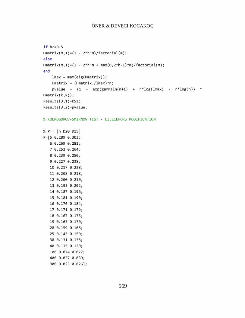
% KOLMOGOROV-SMIRNOV TEST - MARSAGLIA METHOD

k=ceil(n*Dn);

m=2*k-1;

h=k-n*Dn;

Hmatrix=zeros(m,m);

for i=1:m-1

for j=2:m

if i-j+1>=0

Hmatrix(i,j)=1/factorial(i-j+1);

else

Hmatrix(i,j)=0;

end

end

end

for i=1:m-1

Hmatrix(i,1)=(1-h^i)/factorial(i);

end

Hmatrix(m,:)=fliplr(Hmatrix(:,1)');

ÖNER & DEVECI KOCAKOÇ

569

if h<=0.5

Hmatrix(m,1)=(1 - 2*h^m)/factorial(m);

else

Hmatrix(m,1)=(1 - 2*h^m + max(0,2*h-1)^m)/factorial(m);

end

lmax = max(eig(Hmatrix));

Hmatrix = (Hmatrix./lmax)^n;

pvalue = (1 - exp(gammaln(n+1) + n*log(lmax) - n*log(n)) *

Hmatrix(k,k));

Results(3,1)=KSz;

Results(3,2)=pvalue;

% KOLMOGOROV-SMIRNOV TEST - LILLIEFORS MODIFICATION

% P = [n D20 D15]

P=[5 0.289 0.303;

6 0.269 0.281;

7 0.252 0.264;

8 0.239 0.250;

9 0.227 0.238;

10 0.217 0.228;

11 0.208 0.218;

12 0.200 0.210;

13 0.193 0.202;

14 0.187 0.196;

15 0.181 0.190;

16 0.176 0.184;

17 0.171 0.179;

18 0.167 0.175;

19 0.163 0.170;

20 0.159 0.166;

25 0.143 0.150;

30 0.131 0.138;

40 0.115 0.120;

100 0.074 0.077;

400 0.037 0.039;

900 0.025 0.026];

SOME POPULAR GOODNESS OF FIT TESTS FOR NORMALITY

570

aaa=P(:,1)';

subind=max(find(aaa<n));

upind=subind+1;

xxx=P(subind:upind,:);

if aaa(upind)==n

D20=xxx(2,2);

D15=xxx(2,3);

else

D20=xxx(1,2)+(n-aaa(subind))*((xxx(2,2)-xxx(1,2))/(xxx(2,1)-

xxx(1,1)));

D15=xxx(1,3)+(n-aaa(subind))*((xxx(2,3)-xxx(1,3))/(xxx(2,1)-

xxx(1,1)));

end

a1=-7.01256*(n+2.78019);

b1=2.99587*sqrt(n+2.78019);

c1=2.1804661+0.974598/sqrt(n)+1.67997/n;

a2=-7.90289126054*(n^0.98);

b2=3.180370175721*(n^0.49);

c2=2.2947256;

if n>100

D10=(-b2-sqrt(b2^2-4*a2*c2))/(2*a2);

a=a2;

b=b2;

c=c2;

else

D10=(-b1-sqrt(b1^2-4*a1*c1))/(2*a1);

a=a1;

b=b1;

c=c1;

end

if Dn==D10

pvalue=0.10;

elseif Dn>D10

ÖNER & DEVECI KOCAKOÇ

571

pvalue=exp(a*Dn^2+b*Dn+c-2.3025851);

elseif Dn>=D15

pvalue=((0.10-0.15)/(D10-D15))*(Dn-D15)+0.15;

elseif Dn>=D20

pvalue=((0.15-0.20)/(D15-D20))*(Dn-D20)+0.20;

else

pvalue=0.20;

end

Results(4,1)=Dn;

Results(4,2)=pvalue;

% ANDERSON-DARLING TEST

adj=1+0.75/n+2.25/(n^2);

i=1:n;

ui=normcdf(zscore(y),0,1);

oneminusui=sort(1-ui);

lastt=(2*i-1).*(log(ui)+log(oneminusui));

asquare=-n-(1/n)*sum(lastt);

AD=asquare*adj;

if AD<=0.2

pvalue=1-exp(-13.436+101.14*AD-223.73*AD^2);

elseif AD<=0.34

pvalue=1-exp(-8.318+42.796*AD-59.938*AD^2);

elseif AD<=0.6

pvalue=exp(0.9177-4.279*AD-1.38*AD^2);

elseif AD<=153.467

pvalue=exp(1.2937*AD-5.709*AD+0.0186*AD^2);

else

pvalue=0;

end

Results(5,1)=AD;

Results(5,2)=pvalue;

% CRAMER-VON MISES TEST

adj=1+0.5/n;

SOME POPULAR GOODNESS OF FIT TESTS FOR NORMALITY

572

i=1:n;

fx=normcdf(zscore(y),0,1);

gx=(fx-((2*i-1)/(2*n))).^2;

CvMteststat=(1/(12*n))+sum(gx);

AdjCvM=CvMteststat*adj;

if AdjCvM<0.0275

pvalue=1-exp(-13.953+775.5*AdjCvM-12542.61*(AdjCvM^2));

elseif AdjCvM<0.051

pvalue=1-exp(-5.903+179.546*AdjCvM-1515.29*(AdjCvM^2));

elseif AdjCvM<0.092

pvalue=exp(0.886-31.62*AdjCvM+10.897*(AdjCvM^2));

elseif AdjCvM>=0.093

pvalue=exp(1.111-34.242*AdjCvM+12.832*(AdjCvM^2));

end

Results(6,1)=AdjCvM;

Results(6,2)=pvalue;

% SHAPIRO-WILK TEST

a=[];

i=1:n;

mi=norminv((i-0.375)/(n+0.25));

u=1/sqrt(n);

m=mi.^2;

a(n)=-2.706056*(u^5)+4.434685*(u^4)-2.07119*(u^3)-

0.147981*(u^2)+0.221157*u+mi(n)/sqrt(sum(m));

a(n-1)=-3.58263*(u^5)+5.682633*(u^4)-1.752461*(u^3)-

0.293762*(u^2)+0.042981*u+mi(n-1)/sqrt(sum(m));

a(1)=-a(n);

a(2)=-a(n-1);

eps=(sum(m)-2*(mi(n)^2)-2*(mi(n-1)^2))/(1-2*(a(n)^2)-2*(a(n-1)^2));

a(3:n-2)=mi(3:n-2)./sqrt(eps);

ax=a.*y;

KT=sum((x-mean(x)).^2);

b=sum(ax)^2;

SWtest=b/KT;

ÖNER & DEVECI KOCAKOÇ

573

mu=0.0038915*(log(n)^3)-0.083751*(log(n)^2)-0.31082*log(n)-1.5861;

sigma=exp(0.0030302*(log(n)^2)-0.082676*log(n)-0.4803);

z=(log(1-SWtest)-mu)/sigma;

pvalue=1-normcdf(z,0,1);

Results(7,1)=SWtest;

Results(7,2)=pvalue;

% SHAPIRO-FRANCIA TEST

mi=norminv((i-0.375)/(n+0.25));

micarp=sqrt(mi*mi');

weig=mi./micarp;

pay=sum(y.*weig)^2;

payda=sum((y-mean(y)).^2);

SFteststa=pay/payda;

u1=log(log(n))-log(n);

u2=log(log(n))+2/log(n);

mu=-1.2725+1.0521*u1;

sigma=1.0308-0.26758*u2;

zet=(log(1-SFteststa)-mu)/sigma;

pvalue=1-normcdf(zet,0,1);

Results(8,1)=SFteststa;

Results(8,2)=pvalue;

% JARQUE-BERA TEST

E=skewness(y);

B=kurtosis(y);

JBtest=n*((E^2)/6+((B-3)^2)/24);

pvalue=1-chi2cdf(JBtest,2);

Results(9,1)=JBtest;

Results(9,2)=pvalue;

% D'AGOSTINO-PEARSON TEST

beta2=(3*(n^2+27*n-70)*(n+1)*(n+3))/((n-2)*(n+5)*(n+7)*(n+9));

SOME POPULAR GOODNESS OF FIT TESTS FOR NORMALITY

574

wsquare=-1+sqrt(2*(beta2-1));

delta=1/sqrt(log(sqrt(wsquare)));

alfa=sqrt(2/(wsquare-1));

expectedb2=(3*(n-1))/(n+1);

varb2=(24*n*(n-2)*(n-3))/(((n+1)^2)*(n+3)*(n+5));

sqrtbeta=((6*(n^2-5*n+2))/((n+7)*(n+9)))*sqrt((6*(n+3)*(n+5))/(n*(n-

2)*(n-3)));

A=6+(8/sqrtbeta)*(2/sqrtbeta+sqrt(1+4/(sqrtbeta^2)));

squarerootb=skewness(y);

Y=squarerootb*sqrt(((n+1)*(n+3))/(6*(n-2)));

zsqrtbtest=delta*log(Y/alfa+sqrt((Y/alfa)^2+1));

b2=kurtosis(y);

zet=(b2-expectedb2)/sqrt(varb2);

ztestb2=((1-2/(9*A))-((1-2/A)/(1+zet*sqrt(2/(A-

4))))^(1/3))/sqrt(2/(9*A));

DAPtest=zsqrtbtest^2+ztestb2^2;

pvalue=1-chi2cdf(DAPtest,2);

Results(10,1)=DAPtest;

Results(10,2)=pvalue;

% Compare p-value to alpha

for i=1:10

if Results(i,2)>alpha

Results(i,3)=1;

else

Results(i,3)=0;

end

end

% Output display

disp(' ')

ÖNER & DEVECI KOCAKOÇ

575

disp('Test Name Test Statistic p-value Normality

(1:Normal,0:Not Normal)')

disp('----------------------- -------------- --------- ------------

--------------------')

fprintf('KS Limiting Form %6.4f \t %6.4f %1.0f

\r',KSz,Results(1,2),Results(1,3))

fprintf('KS Stephens Modification %6.4f \t %6.4f %1.0f

\r',dKSz,Results(2,2),Results(2,3))

fprintf('KS Marsaglia Method %6.4f \t %6.4f %1.0f

\r',KSz,Results(3,2),Results(3,3))

fprintf('KS Lilliefors Modification %6.4f \t %6.4f %1.0f

\r',Dn,Results(4,2),Results(4,3))

fprintf('Anderson-Darling Test %6.4f \t %6.4f %1.0f

\r',AD,Results(5,2),Results(5,3))

fprintf('Cramer-Von Mises Test %6.4f \t %6.4f %1.0f

\r',AdjCvM,Results(6,2),Results(6,3))

fprintf('Shapiro-Wilk Test %6.4f \t %6.4f %1.0f

\r',SWtest,Results(7,2),Results(7,3))

fprintf('Shapiro-Francia Test %6.4f \t %6.4f %1.0f

\r',SFteststa,Results(8,2),Results(8,3))

fprintf('Jarque-Bera Test %6.4f \t %6.4f %1.0f

\r',JBtest,Results(9,2),Results(9,3))

fprintf('DAgostino & Pearson Test %6.4f \t %6.4f %1.0f

\r',DAPtest,Results(10,2),Results(10,3))