Assignment 2 - Beer Advocate

Teresa Alapat

Samantha Alapat

Ali Minaei

Soham Jatakia

1a) Identify a Data Set to Study

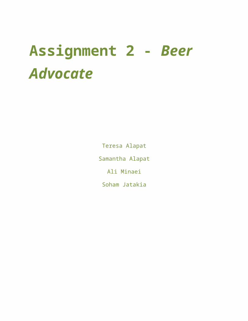
For this assignment we chose to analyze data from BeerAdvocate. Beer Advocate is an online beer rating site which was founded in the year 1996. The data set we used was available at the link: http://snap.stanford.edu/data/Beeradvocate.txt.gz. This dataset had over 1,500,000 data points. A sample data point has the following format:

1b) Exploratory Analysis

As you can see above, there are a total of thirteen features in each data point. Out of these thirteen features, we will perform exploratory analysis to find which of these features are helpful in predicting the 'review/overall' of the beer. We will not be considering the 'review/text' feature because it involves text mining and may take up too much time while not providing that much additional information. During the exploratory analysis, we will focus on the features: 'beer/ABV', 'review/palate', 'review/taste', 'review/aroma', and 'review/appearance'. We will plot graphs of (palate/taste/aroma/appearance) vs ('review/overall') to find the correlation between the subjective ratings and the overall ratings. We will then plot graphs to see if there is a correlation between 'beer/ABV' and the four subjective ratings(palate, taste, aroma, and appearance). This way, we can determine if 'beer/ABV' is an appropriate feature to use. We predict that the four subjective ratings will have a strong influence on the 'review/overall'. We also feel that the

review/appearance': '3' review/profileName': 'stcules' beer/style': 'English Strong Ale' review/palate': '3' review/taste': '3' beer/name': 'Red Moon' beer/ABV': '6.20' beer/beerId': '48213' beer/brewerId': '10325' review/time': '1235915097' review/overall': '3' review/text': 'Dark red color, light beige foam,

average.In the smell malt and caramel, not really light.Again malt and caramel in the taste, not bad in the end.Maybe a note of honey in teh back, and a light fruitiness.Average body.In the aftertaste a light bitterness, with the malt and red fruit.Nothing exceptional, but not bad, drinkable beer.'

review/aroma': '2.5' bad, drinkable beer.',

'beer/ABV' will persuade the 'review/overall' prediction. Below are the graphs we have obtained from our exploratory analysis.

*First we would like to analyze the relationship between the aroma/taste/palate/appearance vs the 'review/overall'. We want to plot these graphs so that we can determine if these four subjective ratings have influence over the 'review/overall' rating. We would expect that if the user gives high aroma, taste, palate, and appearance ratings, that the overall rating would also be high. The graphs are displayed and analyzed starting below.

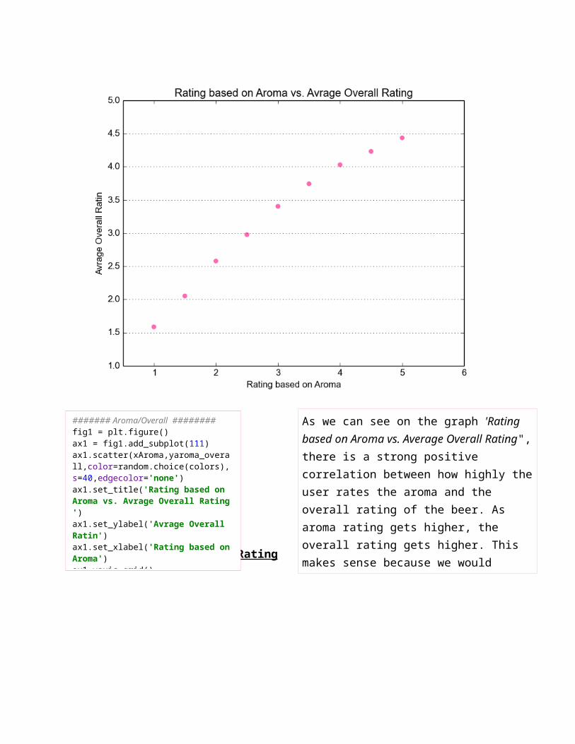
Aroma vs Average Overall Rating

####### Aroma/Overall ########fig1 = plt.figure()ax1 = fig1.add_subplot(111)ax1.scatter(xAroma,yaroma_overall,color=random.choice(colors),s=40,edgecolor='none')ax1.set_title('Rating based on Aroma vs. Avrage Overall Rating ')ax1.set_ylabel('Avrage Overall Ratin')ax1.set_xlabel('Rating based on Aroma')ax1.yaxis.grid()ax1.set_xlim([0.5,6])plt.show()

As we can see on the graph 'Rating based on Aroma vs. Average Overall Rating", there is a strong positive correlation between how highly the user rates the aroma and the overall rating of the beer. As aroma rating gets higher, the overall rating gets higher. This makes sense because we would assume that beers which smell good have higher rating. This relationship indicates that 'review/aroma' is a good feature to use when predicting 'review/overall'.

Taste vs Average Overall Rating

###### taste/overall ########

fig4 = plt.figure()ax4 = fig4.add_subplot(111)ax4.scatter(xtaste,ytaste_overall,color=random.choice(colors),s=40,edgecolor='none')

ax4.set_title('Rating based on Taste vs. Avrage Overall Rating')ax4.set_xlabel('Rating based on Taste')ax4.set_ylabel('Avrage Overall Rating')ax4.yaxis.grid()ax4.set_xlim([0.5,6])plt.show()

As we can see on the graph 'Rating based on Taste vs. Average Overall Rating", there is a strong positive correlation between how highly the user rates the taste of the beer and the overall rating of the beer. As taste rating gets higher, the overall rating gets higher. This makes sense because we would assume that beers which taste good have higher rating. This relationship indicates that 'review/taste' is a good feature to use when predicting 'review/overall'.

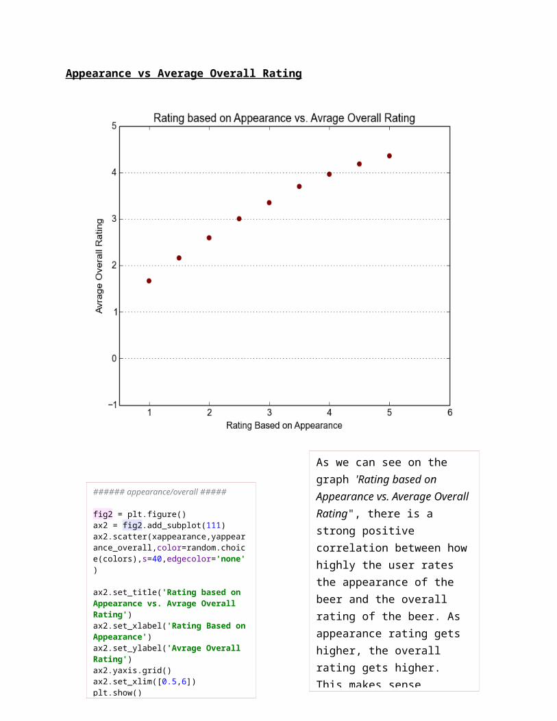
Appearance vs Average Overall Rating

###### appearance/overall #####

fig2 = plt.figure()ax2 = fig2.add_subplot(111)ax2.scatter(xappearance,yappearance_overall,color=random.choice(colors),s=40,edgecolor='none')

ax2.set_title('Rating based on Appearance vs. Avrage Overall Rating')ax2.set_xlabel('Rating Based on Appearance')ax2.set_ylabel('Avrage Overall Rating')ax2.yaxis.grid()ax2.set_xlim([0.5,6])plt.show()

As we can see on the graph 'Rating based on Appearance vs. Average Overall Rating", there is a strong positive correlation between how highly the user rates the appearance of the beer and the overall rating of the beer. As appearance rating gets higher, the overall rating gets higher. This makes sense because we would assume that beers look appealing have higher rating. This relationship indicates that 'review/appearance' is a good feature to use when predicting 'review/overall'.

Palate vs Average Overall Rating

As we observe above, there is a direct, strong correlation between the four subjective ratings(Aroma, taste, appearance, and palate) and the Overall Rating. Thus, four valid features which we can use to predict 'review/overall' are: 'review/taste', 'review/aroma', 'review/appearance', and 'review/palate'. 'Review/palate' seems to be a particularly good feature to use as it shares the strongest relationship with 'review/overall'.

###### palate/overall ########

fig3 = plt.figure()ax3 = fig3.add_subplot(111)ax3.scatter(xpalate,ypalate_overall,color=random.choice(colors),s=40,edgecolor='none')ax3.set_title('Rating based on Palate vs.Avrage Overall Rating')ax3.set_xlabel('Rating Based on Palate')ax3.set_ylabel('Avrage Overall Rating')ax3.yaxis.grid()ax3.set_xlim([0.5,6])plt.show()

As we can see on the graph 'Rating based on Palate vs. Average Overall Rating", there is a strong positive correlation between how highly the user rates palate of the beer and the overall rating of the beer. The palate rating is almost exactly the same as the overall rating (plus or minus .5)! This extremely strong relationship indicates that 'review/palate' is a very good feature to use when predicting 'review/overall'.

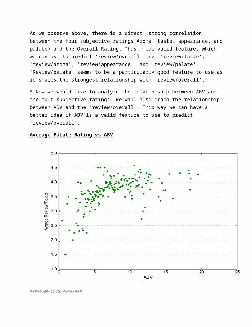
* Now we would like to analyze the relationship between ABV and the four subjective ratings. We will also graph the relationship between ABV and the 'review/overall'. This way we can have a better idea if ABV is a valid feature to use to predict 'review/overall'.

Average Palate Rating vs ABV

##### ABV/palate ########

fig3 = plt.figure()ax3 = fig3.add_subplot(111)ax3.scatter(xABV_palate,yABV_palate,color='green',s=20,edgecolor='none')#ax2.set_ylim([0.5,5.0])ax3.set_xlim([0,25.0])ax3.set_xlabel('ABV')ax3.set_ylabel('Avrage Review/Palate')ax3.yaxis.grid()plt.show()

According to the graph, "Average Palate Rating vs. ABV", it seems like Beers with low ABV content(ABV content between 0 and 5) have lower palate ratings. As ABV content increases, the palate rating generally increases, and peaks at a value of around 4.5.

Average Appearance Rating vs ABV

##### ABV/appearance ########

fig2 = plt.figure()ax2 = fig2.add_subplot(111)ax2.scatter(xABV_appearance,yABV_appearance,color='magenta',s=20,edgecolor='none')#ax2.set_ylim([0.5,5.0])ax2.set_xlim([0,25.0])ax2.set_xlabel('ABV')ax2.set_ylabel('Avrage Review/Appearance')ax2.yaxis.grid()plt.show()

Beers with low ABV content have lower appearance ratings. But as ABV content increases, the rating remains around the value '4'. Beers with ABV level between 0-5 tend to have low appearance ratings, and beers with ABV content greater than 5, tend to have higher appearance ratings (with the average appearance rating being around 4)

Average Taste Rating vs ABV

##### ABV/taste ########

fig4 = plt.figure()ax4 = fig4.add_subplot(111)ax4.scatter(xABV_taste,yABV_taste,color='orange',s=20,edgecolor='none')#ax2.set_ylim([0.5,5.0])ax4.set_xlim([0,25.0])ax4.set_xlabel('ABV')ax4.set_ylabel('Avrage Review/Taste')ax4.yaxis.grid()plt.show()

As the ABV content increases, the average taste rating increases. Beers with ABV content between 0- 5 have low taste ratings and beers with ABV above 5 have higher taste ratings.

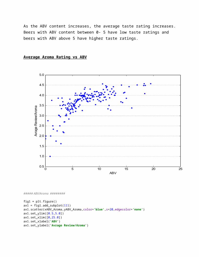
Average Aroma Rating vs ABV

##### ABV/Aroma ########

fig1 = plt.figure()ax1 = fig1.add_subplot(111)ax1.scatter(xABV_Aroma,yABV_Aroma,color='blue',s=20,edgecolor='none')ax1.set_ylim([0.5,5.0])ax1.set_xlim([0,25.0])ax1.set_xlabel('ABV')ax1.set_ylabel('Avrage Review/Aroma')ax1.yaxis.grid()plt.show()

As the ABV content increases, the average aroma rating increases. When the ABV content is between 0 and 5, the aroma rating is lower and when the ABV level is above 5, the aroma rating gets higher and higher as ABV level increases.

Average Review Overall vs ABV

##### ABV/Overall ########

fig5 = plt.figure()ax5 = fig5.add_subplot(111)ax5.scatter(xABV_overall,yABV_overall,color='brown',s=20,edgecolor='none')#ax2.set_ylim([0.5,5.0])ax5.set_xlim([0,25.0])ax5.set_xlabel('ABV')ax5.set_ylabel('Avrage Review/Overall')ax5.yaxis.grid()plt.show()

There is a general positive trend between the review Overall and the ABV content. As the ABV content gets higher, the overall review rating increases. This makes sense because there was a positive trend between the ABV and the four subjective ratings, so it would be natural for there to be a positive trend between the ABV and the overall rating.

After analyzing the results of the exploratory analysis, we can conclude that the features we will be using to predict the 'review/overall' rating are: "beer/ABV", "review/taste", "review/palate", "review/aroma", and "review/appearance". We feel that 'review/palate' will be the most influential feature, since the 'review/palate' was almost identical to the 'review/overall' (plus or minus .5 points).

2) Predictive Task

-Validity of Predictions

In this assignment, our main objective is to predict the 'review/overall' rating of beer. As we concluded from our exploratory analysis, the 'review/overall' is strongly influenced by "review/taste", "review/palate", "review/aroma", and "review/appearance". It is also influenced by "beer/ABV". So, we will use these five features to make the 'review/overall' prediction.

In any predictive task, it is important to test the validity of the prediction and have a way of confirming that they are significant. To do this, we will use a value called "Root Mean Squared Error" (RMSE). RMSE is defined below:

RMSE= [ (1/N) * ∑(fi−yi)^2 ]^(1/2)

where N is the total number of samples, and fi is our prediction of the real value yi ('review/overall') [2]. We will be using a naive simple linear regression model as our baseline model. The baseline model will make a prediction (fi) by taking the average of the 'review/taste', 'review/palate', 'review/aroma' ,and 'review/appearance' of a data point as the single feature in our naive linear regression model. Our goal is to try to create better models which will yield lower RMSE values than the baseline model. That way we can test the validity of our prediction. In this assignment, we are trying to accurately predict the 'review/overall' rating of a beer.

-Preprocessing the Data

* There were a couple steps taken in order to preprocess the data. Firstly we had to convert http://snap.stanford.edu/data/Beeradvocate.txt.gz into a json file. We did this because json files are easier to manipulate in python and are generally more compact.

* We noticed that for some of the data entries in the data set, that the 'beer/ABV' values were empty or missing.

So we deleted the entries with missing 'beer/ABV' values and uploaded a new json file to the share drive (a json file which didn't contain data entries with missing 'beer/ABV' values).

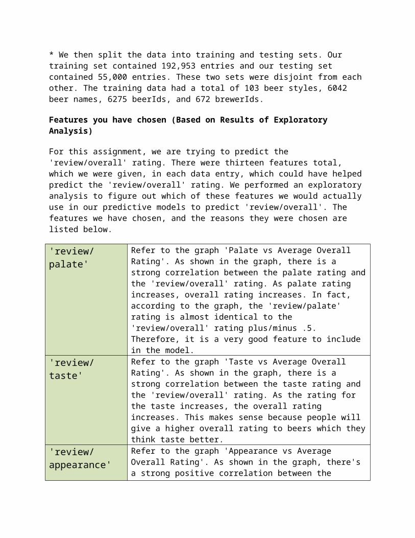
* We then split the data into training and testing sets. Our training set contained 192,953 entries and our testing set contained 55,000 entries. These two sets were disjoint from each other. The training data had a total of 103 beer styles, 6042 beer names, 6275 beerIds, and 672 brewerIds.

Features you have chosen (Based on Results of Exploratory Analysis)

For this assignment, we are trying to predict the 'review/overall' rating. There were thirteen features total, which we were given, in each data entry, which could have helped predict the 'review/overall' rating. We performed an exploratory analysis to figure out which of these features we would actually use in our predictive models to predict 'review/overall'. The features we have chosen, and the reasons they were chosen are listed below.

'review/palate' Refer to the graph 'Palate vs Average Overall Rating'. As shown in the graph, there is a strong correlation between the palate rating and the 'review/overall' rating. As palate rating increases, overall rating increases. In fact, according to the graph, the 'review/palate' rating is almost identical to the 'review/overall' rating plus/minus .5. Therefore, it is a very good feature to include in the model.

'review/taste' Refer to the graph 'Taste vs Average Overall Rating'. As shown in the graph, there is a strong correlation between the taste rating and the 'review/overall' rating. As the rating for the taste increases, the overall rating increases. This makes sense because people will give a higher overall rating to beers which they think taste better.

'review/appearance' Refer to the graph 'Appearance vs Average Overall Rating'. As shown in the graph, there's a strong positive correlation between the appearance rating and the 'review/overall' rating. People give a higher overall rating to beers which they rate higher on appearance.

'review/aroma' Refer to the graph 'Aroma vs Average Overall Rating'. As shown in the graph, there is a strong correlation between the aroma rating and the 'review/overall' rating. This makes sense because people give higher overall ratings to beers which they feel have better aromas.

'beer/ABV' We were not sure if 'beer/ABV' would be a useful feature. However, after the exploratory analysis we found that 'beer/ABV' is correlated to the other four features(palate, taste, appearance, and aroma). As shown in the graph Average Palate Rating vs ABV, beers with low ABV content have lower palate ratings and as ABV content increases, the palate rating generally increases. As shown in the graph Average Appearance Rating vs ABV, we see the trend that beers with low ABV content have lower appearance ratings, but as ABV content increases, the rating remains around the value '4'. If we look at the graph Average Taste Rating vs ABV, we see that the relationship between Taste and ABV is as the ABV content increases, the average taste rating increases. Lastly if we look at the graph Average Aroma rating vs.

ABV, we see that beers with higher ABVs tend to have a higher Aroma rating. Therefore, 'beer/ABV' is a helpful feature in predicting 'Review/overall'

A feature which we thought would help us was 'review/text', however using this as a feature would require us to learn text mining, which would be large learning curve in this short amount of time. So we were not able to use this feature.

3) Select/Design Appropriate Model

Choosing an appropriate model is a very essential part of designing a good predictor. For this assignment we decided to try four different models to predict the 'review/overall'. The models we use are Ridge Regression, Linear Regression, Lasso Regression, and Elastic Net Model. In the following paragraph we will look into the different models more closely.

The Ridge Regression model is a good model for this predictive task because the ridge coefficients minimize a penalized residual sum of squares. The Lasso model is a linear model that estimates sparse coefficients. It is useful in some contexts due to its tendency to prefer solutions with fewer parameter values, effectively reducing the number of variables upon which the given solution is dependent. If two predictors are highly correlated Lasso can end up dropping one rather arbitrarily, that’s why it does not work too well with our predictive task. Elastic-net is useful when there are multiple features, which are correlated with one another. Lasso is likely to pick one of these at random, while elastic-net is likely to pick both. A practical advantage of trading-off between Lasso and Ridge is it allows Elastic-Net to inherit some of Ridge’s stability under rotation.

We considered using other models, one of which was the Least Angle Regression Model. However, Least Angle Regression is used when you are worried about over fitting with linear regression. Since we are not worried about over fitting, we did not use Least Angles Regression. Also, Least Angle Regression is used when you want to fit linear regression models to high-dimensional data [14]. Since the 5 features we are using for the linear regression model are not high dimensional and are in fact collinear, for us, Least Angle Regression will not perform much differently from Linear Regression and therefore would not be a good model to use.

To create a baseline, we considered starting at a point where one would assume that all the useful features are independent of each other and also contribute to the beer rating with a similar magnitude. A naïve way to model this was by taking an average of taste, aroma, appearance, and palate of the beer ratings. Since these features describe the beer properties very well, these were considered above other features. The performance of this kind of a baseline model would be appropriate to test the performance of the other more complicated models.

The dataset we are dealing with, fortunately, does not incorporate noise. The features we used were numbers between 0-5 float values. Some data entries, however, had unknown/missing

information for data labels. For instance, Reviewer/user ID for few of the data entries were missing. We considered this as a viable reason for not using it as a feature. Another example of missing data, is the fact that in a lot of data entries the 'beer/ABV' value was missing. Since we decided that 'beer/ABV' is a useful feature (from our exploratory analysis) we decided to remove the data entries which were missing 'beer/ABV' values and only included the data points which had 'beer/ABV' values. By comparing how well/poorly the four models do in comparison to the baseline we have a better idea of how valid the predictor is.

4) Describe Related Literature

For this assignment we used an existing dataset from BeerAdvocate [4]. BeerAdvocate (BA), was founded in Boston, Massachusetts in the year 1996. It is a global network which is run by a community of professionals and enthusiasts who are dedicated to promoting quality beer. Since its beginning in 1996, BeerAdvocate has become the biggest and most diverse community of beer lovers online [3]. The BeerAdvocate dataset contains reviews which includes ratings in terms of five aspects: appearance, aroma, palate, taste, and overall impression, it also includes information about product and user and a plain text review.[3] BeerAdvocate.com uses this dataset to recommend, rate and review different kinds of beer, bars, and beer stores. Another similar dataset which have been used in the past is the RateBeer dataset which is used by the RateBeer website [1]. The RateBeer data set contains fields such as beer id, aroma, appearance, taste, mouth feel, overall, and comments, and user id. So, in many ways the Rate Beer dataset is very similar to the BeerAdvocate dataset [5]. The RateBeer dataset has been used to obtain the top rated beers, find the most popular beers associated with different countries, find the top beers associated with different seasons, finding brewery information and much more. Another similar dataset is the CraftsCan database. The CraftsCan database is the only database for canned beer on the web [6]. The dataset spans over 2074 beers, 534 breweries, 98 styles and over 51 states. The CraftsCan dataset has information such as beer name, brewery, location (city,state), style, size(in oz), abv, and rating. The CraftsCan website ranks beers according to their style, brewery, and state. Although the CraftsCan dataset is smaller and quite different from the BeerAdvocate and RateBeer datasets, it is still similar in that it is used to rate/rank beers based on different features.

In this assignment, our predictive task is to predict the overall rating or 'review/overall' of a beer. We are using the BeerAdvocate dataset. The BeerAdvocate dataset provides vast data, which includes review ratings (numerical) and textual reviews (text), so many different kinds of models can be used to analyze it.

One such model which can be used to analyze the data from Beer Advocate is the Pale Lager model. This model models the aspects and ratings of aroma, appearance, palate, and taste by analyzing the words used in the textual data. One of the goals of this model is to learn which words are used to describe a particular aspect, and which words are used to describe a particular rating. For example, if we look at the beer advocate data, “the word ‘flavor’ might be used to

discuss the ‘taste’ aspect, whereas the word ‘amazing’ might indicate a 5-star rating. Thus if the words ‘amazing flavor’ appear in a sentence, we would expect that the sentence discusses ‘taste’, and that the ‘taste’ aspect has a high rating” [7]. The Pale Lager model was used in rating prediction task. Many data sets (including Beer Advocate) are missing certain aspect ratings, and the Pale Lager model also has a goal of recovering those missing aspect ratings. This model would be very helpful in predicting a value like "review/overall" because it would make rating predictions based on certain words which are found, and also recover any missing aspect ratings, which is essential to the "review/overall" prediction.

Another model to consider is one which takes into account the idea that a user's experience is a critical underlying factor which effects a user's rating [13]. For example, experienced beer drinkers may rate a certain beer highly (due to acquired taste) while more novice beer drinkers may rate it low (due to inexperience with extreme bitterness). To develop this model, a latent factor recommendation system was used, which took into account a user's level of experience [13]. The standard latent factor model predicted beer rating given a user and item pair. It was found that the model lead to better recommendations. Using this model, it was found that experienced beer raters had less variance in their ratings of beers than beginners. It would have been useful to use this kind of model when predicting 'review/overall'. We could have measured user experience by finding how many times each user-id appeared in the data. Then, we could have implemented a latent factor model which took into account user experience.

The models we talked about above are quite intensive in terms of knowledge and time needed. Instead, we decided to use the four models Linear Regression, Ridge Regression, Lasso Regression, and the Elastic Net model and analyzed which model performed the best on our predictive task. For three of these models, we used Regression analysis. Regression analysis is a process which estimates the relationship between variables. It includes many techniques for modeling and analyzing variables. It focuses on the relationship between the dependent variable ('review/overall') and the predictors ('review/taste', 'review/palate', 'review/aroma', 'review/appearance', 'beer/ABV') [12]. Typically one uses regression analysis for two reasons. First is to predict the value of a dependent variable('review/overall') and second is to estimate the effect of some predictor ('review/taste', 'review/palate', 'review/aroma', 'review/appearance', 'beer/ABV') on the dependent variable.

We decided to use Linear Regression as one of the four models used to predict 'review/overall'. Our explanatory variables were 'review/taste', 'review/palate', 'review/aroma', 'review/appearance' and 'beer/ABV'. Our dependent variable was 'review/overall'. We believe that this linear regression model will perform well because the four subjective ratings and strong influences on the dependent variable and 'beer/ABV' is a useful feature due to its influence on the four subjective ratings, which was discovered during the exploratory analysis. Apart from linear regression we decided to use two more regression models: Ridge Regression and Lasso Regression.

Both Lasso Regression and Ridge Regression are regularized methods which can prevent overfitting [10]. Overfitting is a modeling error which occurs when a function is too closely fit to a limited set of data points. Ridge regression usually has a better compromise between bias and variance [11]. It uses the L2 norm for regularization. However, it cannot zero out coefficients for predictors like Lasso Regression. Lasso Regression can zero out irrelevant variables. It uses the L1 norm for regularization. However, Lasso Regression tends to do worse when there is high co linearity between the predictors [11]. This is the case for our predictors, because as we observed in the exploratory analysis, (aroma rating, taste rating, appearance rating, palate rating, and overall rating) are all correlated with one another. So, we believe that the Ridge Regression Model will yield more accurate results than the Lasso Regression Model. We predict that Ridge Regression and Linear Regression will yield about the same accuracy.

We additionally decided to use the Elastic Net model to predict ‘review/overall’. The main difference between Lasso Regression and Ridge Regression is the penalty term they each use. Ridge uses the L2 penalty term which limits the size of the coefficient vector, while Lasso Regression uses the L1 penalty term which imposes sparsity among the coefficients and therefore makes the fitted model easier to interpret. Elastic Net is introduced as a compromise between these two techniques, and has a penalty which is a mix of L1 and L2 norms [14]. Therefore, since Elastic Net Model linearly combines L1 and L2, we expect the Elastic Net Model to have a performance between the Ridge Regression Model and the Lasso Model. We decided to use Elastic Net Model to see how it performs and to see whether our predictions were correct.

5) Conclusion

We used four models to predict 'review/overall'. They were Linear Regression Model, Ridge Regression Model, Lasso Regression Model, and Elastic Net Model. We calculated the RMSE when using each of these models on the test dataset and training data set and compared it to the baseline RMSE values. The Linear Regression and Ridge Regression Models performed better than the baseline, and the Lasso Regression and Elastic Net Model performed worse than the baseline. The performance of these models with respect to each other, are listed below.

Model Training RMSE Testing RMSE

Baseline 0.441768917803 0.448951979883

Linear Regression

0.401544613578 0.403819420589

Ridge Regression

0.401544613705 0.403819420589

Lasso Regression

0.620528401458 0.598084785606

Elastic Net 0.520744894393 0.515477705735

The baseline model for this assignment was a simple linear regression model. A simple linear regression model is a linear regression model with a single explanatory variable. The outcome variable ('review/overall') depends only on a single predictor [9]. The single predictor we are using for the baseline model is the average of the 'review/appearance', 'review/aroma', 'review/palate', and 'review/taste'. So, for each data point, we predict that the 'review/overall' value will be equal to the average of the four subjective ratings of that data point. As shown in the table above, the Baseline model had an RMSE value of 0.441768917803 on the training data and an RMSE value of 0.448951979883 on the testing data. The theta vector of the baseline model was [0.15266869, 0.96681848]. As expected the single explanatory variable has a very high theta value (.9668) because it has high influence on the outcome variable. We wanted to see how the other model performed compared to the baseline model.

The Linear Regression Model and the Ridge Regression model performed with the same accuracy on the testing and training set. The RMSE value of the training data was around 0.401544613578 (the two RMSE values start differing on the 10th decimal place) and the RMSE value for the test data was 0.403819420589 (for both models). The theta vector for the Linear Regression Model and the Ridge Regression Model was [0, -0.04243654, 0.05861982, 0.08870169, 0.27325455, 0.5433695]. From the theta vector we can see that the taste of a beer has high influence (.5433) on the overall rating of the beer. We can see that the ABV has the least influence (-.042) on the overall rating of the beer. Appearance, aroma and palate have similar influence on the overall rating of the beer, with Palate having a slightly higher influence of (.273), about half the influence of taste! We thought that these results made sense because we thought that the taste of the beer would have most influence on its overall rating, after all, people generally tend to rate beers which taste good very highly. We also thought that it made sense that the ABV had less influence on the overall rating of a beer because when doing exploratory analysis, the ABV had a less defined relationship with the overall rating of the beer and the four subjective ratings.

The Lasso Regression Model performed worse than the Baseline. The RMSE on the training set was 0.620528401458 and the RMSE on the test set was 0.598084785606. The Lasso model is a linear model that estimates sparse coefficients. It is useful in some contexts due to its tendency to prefer solutions with fewer parameter values, effectively reducing the number of variables upon which the given solution is dependent. However, If two predictors are highly correlated/collinear, Lasso can end up dropping one rather arbitrarily, that’s why it does not work too well with our predictive task. Most of our predictors are collinear. In fact, if you look at the theta values, there is proof of this, as we only have four theta values which means that this model only considered four features instead of five features. This means that the Lasso model ended up arbitrarily dropping one of the predictors. Therefore, the Lasso Model was not a good model to use for our prediction task.

We hypothesized that the Elastic Net Model would perform between the Ridge Regression Model and the Lasso Regression Model and we were correct. The RMSE value of the Elastic Net model on the training set was 0.520744894393 and the performance on the test set was 0.515477705735. This is the average of the RMSE values of the Ridge Regression Model and the Lasso Regression Model! The theta values for the Elastic Net Model was [0, 0.07931763, 0.16474125, 0.14920616, 0.21682921, 0.28563037]. The RMSE of the Elastic Net Model on training data is 0.520744894393, which is the mean of the RMSE of the Ridge Regression Model, 0.401544613705, and the RMSE of the Lasso Regression Model, 0.620528401458. Since the Elastic Net Model is the exact mean between Lasso Model and Ridge Model, and linearly combines L1 and L1 penalties, we can say that L1 and L2 have about equal influence and do not sway the RMSE value more towards the performance of Lasso Regression or Ridge Regression. However, the Elastic Net Model still performs quite poorly with respect to the baseline and we do not consider it a good model for this prediction task.

In this assignment we used four different models to predict the 'review/overall' rating of a beer. We performed exploratory analysis by plotting relationships between the different features on graphs and decided the features that we were going to use were 'review/palate', 'review/taste' , 'review/aroma', 'review/appearance' and 'beer/ABV'. We found that the Linear Regression Model and the Ridge Regression Model performed well and that the 'review/taste' and 'review/palate' were the most influential features (by looking at the theta vector). So if a beer tastes good, it is a big indicator that it will have a high overall rating. We also found that the Lasso Regression Model did not perform well (due to the fact that the predictors we were using were collinear/correlated) and the Elastic Net Model performed poorly (it performs on average, between Ridge Regression and Lasso Regression). From this assignment we learned that even if you choose good features (like the four subjective ratings, and the beer/ABV) the relationship between those features (like if they are highly correlated or not) are crucial when deciding which model you are going to use for the predictive task. This assignment helped us learn how to perform exploratory analysis to discover which features are useful and how to design and analyze models to solve a predictive task.

References

[1] Rate Beer Dataset: http://snap.stanford.edu/data/Ratebeer.txt.gz

[2] "Mean Squared Error and Residual Sum of Squares." Mse. N.p., n.d. Web. 30 Nov. 2015. <http://stats.stackexchange.com/questions/73540/mean-squared-error-and-residual-sum-of-squares>.

[3] "Welcome to BeerAdvocate (BA). Respect Beer.™." BeerAdvocate. N.p., n.d. Web. 30 Nov. 2015. <http://www.beeradvocate.com/>.

[4] Beer Advocate Dataset: http://snap.stanford.edu/data/Beeradvoc

ate.txt.gz

[5] "RateBeer API." RateBeer JSON API Documentation. N.p., n.d. Web. 30 Nov. 2015. <http://www.ratebeer.com/json/ratebeerapi.asp>.

[6] "CraftCans.com - News and Reviews for the Canned Beer Revolution." CraftCans.com. N.p., n.d. Web. 30 Nov. 2015. <http://www.craftcans.com/>.

[7] Mcauley, Julian, Jure Leskovec, and Dan Jurafsky. "Learning Attitudes and Attributes from Multi-aspect Reviews." 2012 IEEE 12th International Conference on Data Mining (2012): n. pag. Web.

[9] "When to Use Regularization Methods for Regression?" Least Squares. N.p., n.d. Web. 30 Nov. 2015. <http://stats.stackexchange.com/questions/4272/when-to-use-regularization-methods-for-regression>.

[10] "Regression Analysis: An Overview." Regression Analysis: An Overview. N.p., n.d. Web. 30 Nov. 2015. <http://www.kellogg.northwestern.edu/faculty/weber/emba/_session_2/regression.htm>.

[11] "When to Use Regularization Methods for Regression?" Least Squares. N.p., n.d. Web. 30 Nov. 2015. <http://stats.stackexchange.com/questions/4272/when-to-use-regularization-methods-for-regression>.

[12] Wikipedia. Wikimedia Foundation, n.d. Web. 30 Nov. 2015. <https://en.wikipedia.org/wiki/Regression_analysis>.

[13] Mcauley, Julian, Jure Leskovec, and Dan Jurafsky. "Learning Attitudes and Attributes from Multi-aspect Reviews." 2012 IEEE 12th International Conference on Data Mining (2012): n. pag. Web.

[14] "Ridge, Lasso and Elastic Net." References. N.p., n.d. Web. 01 Dec. 2015.