Embed Size (px)
Citation preview
7/23/2019 job scheduling 2
http://slidepdf.com/reader/full/job-scheduling-2 1/8
Moth/ Compuf. Modelling Vol. 13 No. 3 pp. 29-36 1990
Printed n Great Britain
089s7177/90 3.00 + 0.00
PergamonPress
plc
SCHEDULING GROUPS OF J OBS IN THE
TWO MACHINE FLOW SHOP?
K. R.
BAKER
The Amos Tuck School of Business Administration, Dartmouth College, Hanover, NH 03755, U.S.A.
Abstract This paper provides a review of the two-machine flow shop model when time lags or setups
are introduced. Building on these results, it establishes a general framework for scheduling groups of jobs
when each group requires a setup.
INTRODUCTION
Scheduling models for groups of jobs have gained significance as group technology (GT) has
become more widely applied. In the GT scheduling problem there is typically an incentive to
perform similar tasks together and a requirement to incur a setup in order to perform a dissimilar
task. Many basic models for the scheduling of independent jobs have been extended to the GT
setting. For example, the minimization of mean flowtime is treated by Yoshida et al. [l], and the
minimization of mean tardiness is examined by Yoshida et al. [2] and Ozden et al. [3]. Each of these
papers deals with a single-machine model.
The flow shop model is analyzed by Yoshida and Hitomi [4,5], and their result is reported in
the survey of Ham et al. [6]. However, they consider one variation of many that can occur in the
GT environment. The purpose of this paper is to develop a general framework within which several
variations of the GT model can be analyzed for the two-machine flow shop.
In order to provide the base for this framework, we review the important results on flow shop
scheduling with time lags. This review states certain key properties that have not been discussed
in the basic papers on this topic. We pay particular attention to the possible overlapping of tasks.
We also distinguish anticipatory (or “separable”) setups from nonanticipatory setups. Although
these two features are not always explicit in scheduling models, they appear at first glance to
generate different problems. However, the general framework we present here permits us to handle
several variants with one basic scheduling rule.
The results we cover pertain to the two-machine model. Of course, the restriction to two
machines is limiting, but we know that many interesting and practical m-machine problems are
quite difficult to solve. The m-machine version of the GT scheduling problem considered here is
likely to be even more difficult. However, the optimal solution to two-machine problems has often
supplied the kernel from which a general solution technique has been developed. Two well-known
examples are the flow shop heuristic of Campbell
et al.
[7] and the branch-and-bound procedure
of Lageweg
et al. [8].
In the same vein, we expect that the insights gained in solving two-machine
GT problems will be useful in attacking larger ones. This same analogy has already been
demonstrated in the work of Ham et al. [6, Chap. 81.
THE TWO-MACHINE FLOW SHOP MODEL
In order to describe the basic flow shop model, let uj denote the processing time of job j on
machine 1 and let
bj
denote the time on machine 2, where precedence requirements dictate that jobs
must go to machine 1 before machine 2. Indeed, in the basic model, each job must complete all
of its work on machine 1 before it starts on machine 2. The objective is to minimize the schedule
length, or
makespan.
The fundamental result for flow shop sequencing [9] states that in this basic
model, job i precedes job i in an optimal sequence if
min(a,, b,) -c min(u,, bi).
1)
tworking paper No. 231 from the Amos Tuck School of Business Administration.
29
7/23/2019 job scheduling 2
http://slidepdf.com/reader/full/job-scheduling-2 2/8
30 K. R.
BAKER
(al
(b)
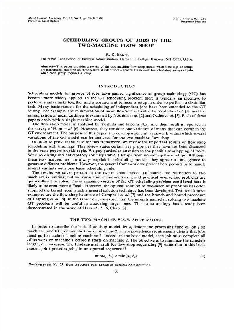
Fig. 1. Right-shifting to avoid inserted idle time.
This ordering allows a complete sequence to be constructed by ranking the job processing times,
starting with the shortest, and breaking ties arbitrarily. The job corresponding to the first
processing time on this list is placed in the first or last available position in sequence, according
to whether the processing time is on machines 1 or 2, respectively. That job is then removed from
consideration, and the remaining list is treated the same way, until all jobs are sequenced.
Normally, when the flow shop model is presented in the literature, diagrams of schedules
produced by Johnson’s rule suggest that each operation should be scheduled as early as possible
on each machine. As a result, there is no idle time on machine 1 until all jobs have been processed,
but there may be inserted idle time on machine 2. See Fig. l(a) for such an example. Notice that,
as long as our objective is to minimize makespan, we can also schedule the jobs on machine 2 so
that there is no inserted idle time once processing begins. This simply involves right-shifting the
operations of machine 2 as they appear in Fig. l(a), while maintaining the completion time of the
last operation. Figure l(b) depicts the modification, where i, denotes the idle time on machine 2
before processing begins and i, denotes the idle time on machine 1 after processing is complete.
For convenience, we refer to these respectively as the initial
and
f inal idle times of the schedule.
To compute these quantities, let
yk = (al + a2 + ’ ..+ak)- b,+b,+,..+6,_,).
2)
The two sums in equation (2) represent the machine workloads that must be completed prior to
the processing of job k at machine 2. Their difference represents the amount of initial idle time
necessary on machine 2 prior to the processing of jobs 1 through k, given that they are processed
without inserting idle time. The quantity yk is a lower bound on i,. Thus,
In symmetric fashion let
x, = (bk +
where n is the number of jobs
i, = max( yk).
b,+, +.. ‘+b,)- ak+,+ak+z+...+a,),
in the schedule. Then
i2 = max(x,).
(3)
(4)
(5)
We shall generalize these definitions later on.
THE MODEL WITH TIME LAGS
Time lags (start lags and stop lags) are discussed by Mitten [lo] and several other authors,
leading to the general models presented by Rinnooy Kan [l l] and Szwarc [12]. The motivation for
introducing start and stop lags is to allow for splitting and overlapping of jobs. That is, processing
can begin at machine 2 on an early portion of a job, while the later portion is still at machine 1.
A typical application would be a situation where each job is a batch consisting of several discrete
and identical units. Once the first unit completes at machine 1, it can immediately begin processing
at machine 2. In this case, the start lag represents the time to process one unit on machine 1, and
the stop lag represents the time to process one unit on machine 2. In other words, we would be
using a “transfer batch” of size 1. Obviously, transfer batches of size > 1 can also be modeled with
the use of time lags. In particular, define a start lag uj as the required delay between the start of
the first operation and the start of the second operation. Analogously, a stop lag Uj s the required
delay between the completion of the first operation and the completion of the second. As shown
7/23/2019 job scheduling 2
http://slidepdf.com/reader/full/job-scheduling-2 3/8
The two-machine flow shop model
(b)
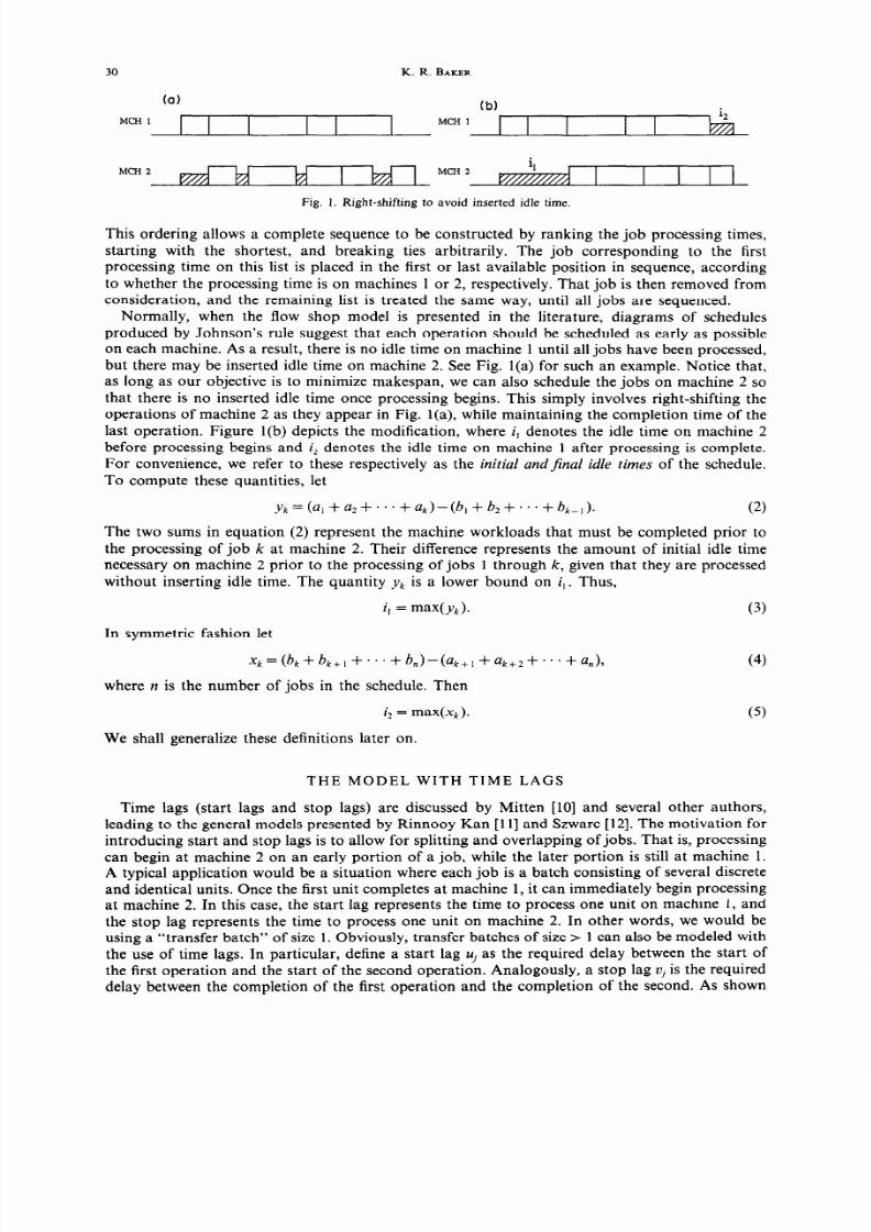
Fig. 2. The relationships among time-lags and processing times.
by Rinnooy Kan [l 11 he optimal schedule is characterized by a rule analogous to condition (1):
specifically, job
i
precedes job j in an optimal sequence if
min(a, + dii, b, + d,) < min(u, + d,, bi + di),
6)
where
d, = max(u,- aj, oj- b,).
(7)
The form of equation (7) in which d, may be negative, reflects the fact that one of the two time
lags will always be binding. If, as in Fig 2(a), we have
d, = uj -a, > v,-b,,
then the start lag is binding, and a schedule that meets the start-lag constraint will automatically
satisfy the stop-lag constraint. On the other hand, if, as in Fig. 2(b), we have
d,= v,-b,> uj-a/,
then the stop-lag is binding, and a schedule that meets the stop-lag constraint will automatically
satisfy the start-lag constraint. In either case, d, represents the time offset between the completion
of the first operation and the start of the second operation. Conway et al. [13] referred to 4. as
the transfer lag.
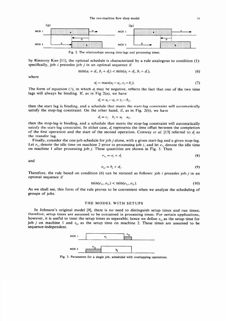
Finally, consider the one-job schedule for jobj alone, with a given start-lag and a given stop-lag.
Let e,j denote the idle time on machine 2 prior to processing job j, and let e,, denote the idle time
on machine 1 after processing job j. These quantities are shown in Fig. 3. Then
e,, = aj + d,
8)
and
e2,=
bj+dj.
9)
Therefore, the rule based on condition (6) can be restated as follows: job i precedes job i in an
optimal sequence if
min(e,,, ezj) < min(e,j, ezi).
(10)
As we shall see, this form of the rule proves to be convenient when we analyze the scheduling of
groups of jobs.
THE MODEL WITH SETUPS
In Johnson’s original model [9], there is no need to distinguish setup times and run times;
therefore, setup times are assumed to be contained in processing times. For certain applications,
however, it is useful to treat the setup times as separable; hence we define slj as the setup time for
job j on machine 1 and sSj as the setup time on machine 2. These times are assumed to be
sequence-independent.
Fig. 3. Parameters for a single job, scheduled with overlapping operations.
7/23/2019 job scheduling 2
http://slidepdf.com/reader/full/job-scheduling-2 4/8
32 K. R.
BAKER
(al
tb)
........
.......
1
lj
aj
Sl.
J
aj
‘ j
bj j
bj
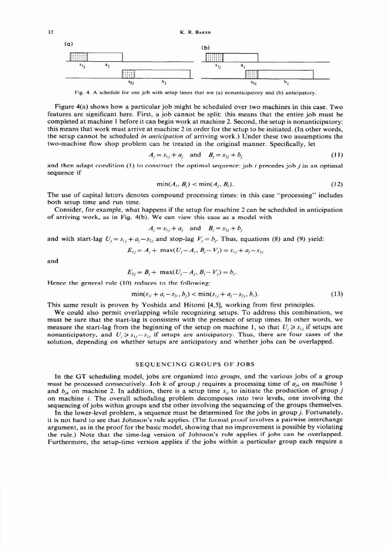
Fig. 4. A schedule for one job with setup times that are (a) nonanticipatory and (b) anticipatory.
Figure 4(a) shows how a particular job might be scheduled over two machines in this case. Two
features are significant here. First, a job cannot be split: this means that the entire job must be
completed at machine 1 before it can begin work at machine 2. Second, the setup is nonanticipatory:
this means that work must arrive at machine 2 in order for the setup to be initiated. (In other words,
the setup cannot be scheduled in ant icipat ion of arriving work.) Under these two assumptions the
two-machine flow shop problem can be treated in the original manner. Specifically, let
Aj = slj + a, and E, = sIi i b,
1 I)
and then adapt condition (1) to construct the optimal sequence: job
i
precedes
job j
in an optimal
sequence if
min(Ai, B,) < min(A,,
B,).
(12)
The use of capital letters denotes compound processing times: in this case “processing” includes
both setup time and run time.
Consider, for example, what happens if the setup for machine 2 can be scheduled in anticipation
of arriving work, as in Fig. 4(b). We can view this case as a model with
Aj = s,, + aj
and
B, = szi + b,
and with start-lag U, = slj + a,-szj and stop-lag V, = by Thus, equations (8) and (9) yield:
E,j= A,+ max(U,-Aj, B,- V,)
=~,,+a,-s~~
and
Ezj= B,+ max(U,-A,, B,- V,) = b,
Hence the general rule (10) reduces to the following:
min(s,, + a, s,, b,) < min(sli + a/- sz,, b,).
(13)
This same result is proven by Yoshida and Hitomi [4,5], working from first principles.
We could also permit overlapping while recognizing setups. To address this combination, we
must be sure that the start-lag is consistent with the presence of setup times. In other words, we
measure the start-lag from the beginning of the setup on machine 1, so that U, > slj if setups are
nonanticipatory, and Uj > slj--s,, if setups are anticipatory. Thus, there are four cases of the
solution, depending on whether setups are anticipatory and whether jobs can be overlapped.
SEQUENCING GROUPS OF JOBS
In the GT scheduling model, jobs are organized into
groups,
and the various jobs of a group
must be processed consecutively. Job k of group j requires a processing time of
ajk
on machine 1
and bjk on machine 2. In addition, there is a setup time s,~ to initiate the production of group j
on machine
i .
The overall scheduling problem decomposes into two levels, one involving the
sequencing of jobs within groups and the other involving the sequencing of the groups themselves.
In the lower-level problem, a sequence must be determined for the jobs in group j. Fortunately,
it is not hard to see that Johnson’s rule applies. (The formal proof involves a pairwise interchange
argument, as in the proof for the basic model, showing that no improvement is possible by violating
the rule.) Note that the time-lag version of Johnson’s rule applies if jobs can be overlapped.
Furthermore, the setup-time version applies if the jobs within a particular group each require a
7/23/2019 job scheduling 2
http://slidepdf.com/reader/full/job-scheduling-2 5/8
The two-machine flow shop model
33
minor setup. Assuming that the lower-level problem has been solved, we use the subscript to mean
the kth job in the optimal sequence for the group.
In the higher-level problem, a sequence must be determined for the groups. The essential
modeling question here is how to redefine groups as pseudo-jobs in order to apply the existing
results of flow shop theory. Clearly, if setup times are nonanticipatory and groups must each
complete work on machine 1 before starting on machine 2, then we can simply redefine groups
as jobs and use Johnson’s rule. Formally, let
and
Aj =
Slj +
1 alk
k
Then group i precedes job j in an optimal sequence if
min(A,,
B,) <
min(Aj,
B;).
Similarly, if we prohibit the overlapping of groups but permit anticipatory setups, then we can
adapt condition (13) to yield an optimal sequence.
However, the essence of the typical GT scheduling problem is that groups can be processed in
overlapping fashion, because one of the jobs in the group can occupy machine 2 while another
occupies machine 1. For this reason, our general framework must recognize that groups could
overlap. To allow for overlapping we invoke the time-lag model, with groups in the role of what
were jobs. Hence, the basic rule governing the sequence of groups is the following: group i precedes
group j in an optimal sequence if
min(A, + D i , B, + 0,) < min(Aj + Dj , Bi + Di ),
(14)
where the parameters in this expression refer to properties of groups, being determined from the
problem data and assumptions about setups, as we discuss next.
Assume first that setups are nonanticipatory and that jobs must complete on machine 1 before
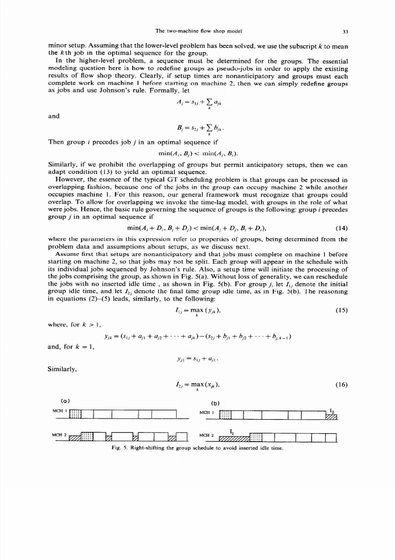
starting on machine 2, so that jobs may not be split. Each group will appear in the schedule with
its individual jobs sequenced by Johnson’s rule. Also, a setup time will initiate the processing of
the jobs comprising the group, as shown in Fig. 5(a). Without loss of generality, we can reschedule
the jobs with no inserted idle time ,
as shown in Fig. 5(b). For groupj, let Ilj denote the initial
group idle time, and let Z2j denote the final time group idle time, as in Fig. 5(b). The reasoning
in equations (2)-(j) leads, similarly, to the following:
where, for k > 1,
I,, = my (Y,~), (15)
_Y,k (SI, + ajl + aj2 + .
+a,,)- S,,+b,,+bj ,+...+b,,k_,)
and, for
k =
1,
Similarly,
Yjl slj + ql.
12, = m;x -u,)~
16)
(a)
(b)
MCH 1 ::::::
MCHZ
I, ......
d I I
Fig. 5. Right-shifting the group schedule to avoid inserted idle time.
7/23/2019 job scheduling 2
http://slidepdf.com/reader/full/job-scheduling-2 6/8
34
K. R BAKER
where, for k > 1,
Xjk = b jk+b j ,k+ I+“ ‘ +b jg ) - u j .k+ ,+U j ,k+ ,+” ’+Qjg )
and, for k = 1,
XII= (Szj+ bj, + bj2 +
’ ’ . +
bjg)- ~j , + U j3 . . +
U,g),
where g is the number of jobs in the group.
With these definitions in place, we can interpret Z,j as the start-lag for group j, and Zzj s the
stop-lag. The parameters are therefore as follows:
Aj = Slj + 1
ajk
k
B j = S2 j + C
bjk
k
u, = I,j
and
and so
D,=max(U,-Aj,
y--B,)
= max max y,k)-slj-~ ajk,
maX Xjk)-s2j-~
bjk
i
.
k k
Although the optimal sequence can be obtained from condition (14) with the parameters in this
form, it turns out that an alternative version exists, just as condition (10) serves as an alternative
to condition (6) for the sequencing of jobs. With analogous reasoning it can be shown that
and
Aj+D,=Z,j
B, + Dj = Izr.
Therefore the optimizing rule may be stated as follows:
group i precedes group j i n an optimal
sequence i f
min I,i, Izj ) < mi n Z,j, Z2,).
17)
If setups are anticipatory, this same rule applies, but the yjk and xjk must be calculated
consistently. In equation (15), we have, Vk 2 1,
y jk = SI, + aj l + uj 2 + ’ ’ .+Ujk ) - S,j+bj ,+b,,+.. .+b,,k_,) .
In equation (16) we must take the maximum for k > 0, where, for k > 1,
Xjk= bjkkbj.k+,+“‘+bj~)- Uj,k+,fUj,k+,+.”+Uj~)
and, in addition,
Xj o= szj+bjl +bjz+..
’ + b,k_,) - Slj + ujl +
U,2 f . . ’ + Ujk).
Finally, the result in condition (17) can be extended to overlapping jobs by specifying the
calculation of yjk and xjk appropriately.
EXAMPLE
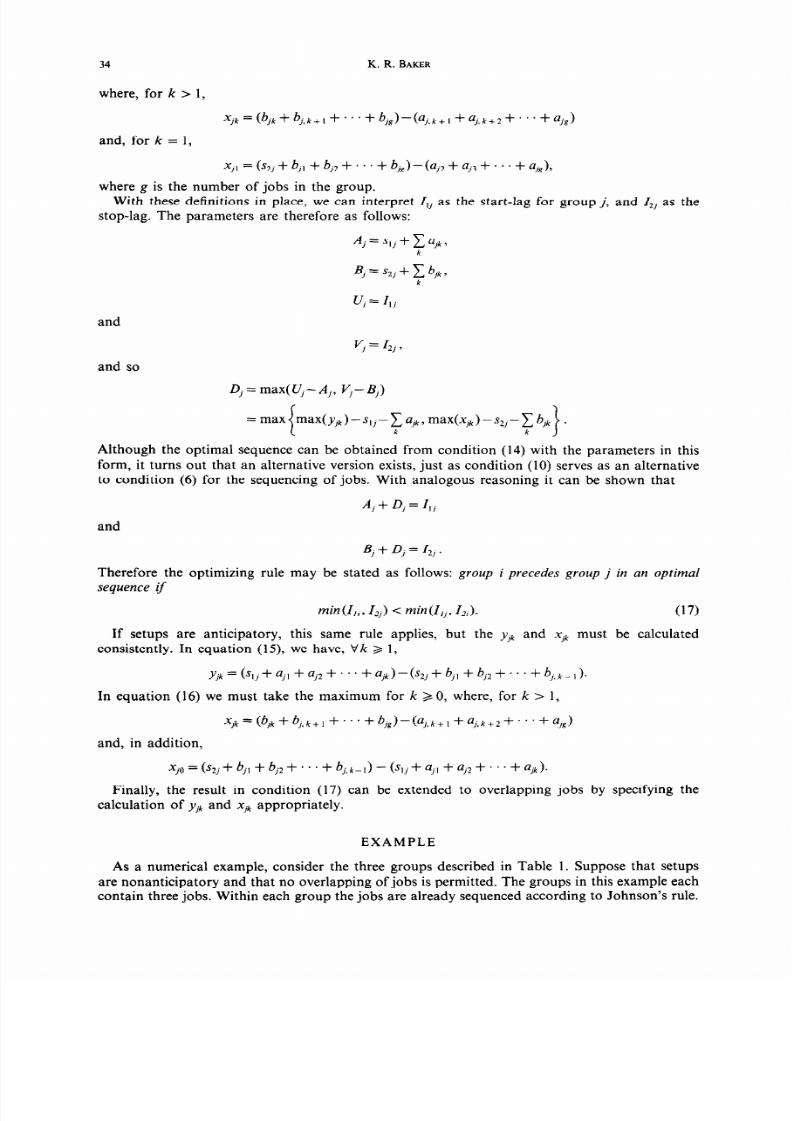
As a numerical example, consider the three groups described in Table 1. Suppose that setups
are nonanticipatory and that no overlapping of jobs is permitted. The groups in this example each
contain three jobs. Within each group the jobs are already sequenced according to Johnson’s rule.
7/23/2019 job scheduling 2
http://slidepdf.com/reader/full/job-scheduling-2 7/8
The two-machine flow shop model
Table 1. An example containing three groups and nine jobs, with setup times and
processing times given; for the case of nonanticipatory setups, the I,, values are
computed from the given information
Gr0tlp/ Setup
machine times
Process times
I,, and 12,
values
l/l 5 5 II 8 10
112 10 8 12 6 17
20 8 3 5 7 11
212 IO 6 5 3 12
30 5 3 8 16 8
312 2 12 15 4 9
35
Table 2. An example containing three groups and nine jobs, with setup times and
processing times given; for the case of anticipatory setups, the I, values are
computed from the given information
Group/
Setup
I,, and rI,
machine
times
process times values
l/l 5 5 II 8 3
112 10 8 12 6 IO
20 8 3 5 7 2
2/2 10 6 5 3 3
3/l 5 3 8 16 6
312 2 12 15 4 7
The table summarizes the required calculations with the values of Z,j and I,. These values imply
an optimal group sequence of 3-l-2, as can be verified from the summary of Z-values shown
below:
Group j 1 3 2
Ilj 8 10 11
I
2J
9 17 12
The makespan for the entire schedule is 102.
Now suppose that setups are anticipatory in the same example. Table 2 contains a set of
appropriate calculations, showing the change in the value of I,,. As should be clear from Fig. 5,
the difference between I,j and IIj is unaffected by the change in the assumption about setups.
However, there may still be an incentive to resequence the groups. In this case the optimal
sequences is 2-l-3, as can be verified from the summary of Z-values shown below:
Group j 2 3
1
[lj
2
3 6
I
2,
3 10 7
The makespan for this schedule is 95.
SUMMARY
We have analyzed the two-machine flow shop model involving groups of jobs. Each group
requires a setup on each machine, in order to initiate the processing of the jobs in the group. The
first step in the solution (the lower-level problem) is to order the jobs in each group according to
Johnson’s rule. The next step is to calculate the initial group idle time Z,j and the final group idle
time Z,, based on this ordering of jobs. Finally, in the higher-level problem, the groups are
sequenced according to the following rule: group
i
precedes group i if min(Zli, Ztj) < min(Z,j, Zzi).
This ordering allows a complete sequence to be constructed by ranking the group idle times, starting
with the shortest, and breaking ties arbitrarily. The group corresponding to the first idle time on
this ranked list is placed in the first or last available position in sequence according to whether the
idle time is initial or final, respectively. That group is then removed from consideration, and the
remaining list is treated the same way until all groups are sequenced.
7/23/2019 job scheduling 2
http://slidepdf.com/reader/full/job-scheduling-2 8/8
36
K. R.
B KER
The results in this paper generalize Theorem 1 of Kurisu [14], regarding the sequencing of strings
of jobs. Our framework can be viewed as a generalization of the rule in condition (10) for
sequencing overlapping jobs to the sequencing of overlapping groups. As we have seen, the rule
is unchanged if we assume that group setup times are anticipatory instead of nonanticipatory, or
if we assume that individual jobs can be split and overlapped, or if we assume that individual jobs
require minor setups. The only differences occur in the applications of Johnson’s rule to the
lower-level problem and in the specific calculation of Zij.
Acknowledgements-The comments of Professor W. Szwarc and an anonymous referee on earlier drafts of this manuscript
are gratefully acknowledged.
REFERENCES
1. T. Yoshida, N. Nakamura and K. Hitomi, A study of production scheduling (optimization of group scheduling on
a single production stage). Trans. Japan Sot. mech. Engng 39, 1993-2003 (1973).
2. T. Yoshida, N. Nakamura and K. Hitomi, Group production scheduling for minimum total tardiness. AIIE Trans.
10, 157-162 (1978).
3. M. Ozden, P. Egbelu and A. Iyer, Job scheduling in a group technology environment for a single facility.
Computers
ind . Engng 9, 67-72 1985).
4.
T. Yoshida and K. Hitomi, Multi-stage production scheduling with setup time consideration.
Trans. Japan Sot. mech.
Engng 45 395) 1979).
5. T. Yoshida and K. Hitomi, Optimal two-stage production scheduling with setup times separated. AIIE Trans. 11,
261-263 (1979).
6. I. Ham, K. Hitomi and T. Yoshida,
Group Technology.
Kluwer-Nijhoff, Amsterdam (1985).
7. H. G. Campbell, R. A. Dudek and M. L. Smith, A heuristic algorithm for the n job, m machine sequencing problem.
Mgmt Sci. 16, B630-637 (1970).
8. B. J. Lageweg, J. K. Lenstra and A. H. G. Rinnooy Kan, A general bounding scheme for the permutation flow shop.
Ops Res.
26, 53-67 (1978).
9. S. M. Johnson, Optimal two- and three-stage production schedules with setup times included. Nav. Res. Logist. Q. 1,
61-68 (1954).
10. L. G. Mitten, Sequencing n jobs on two machines with arbitrary time lags. Mgmt Sci. 5, 293-298 (1959).
Il. A. H. G. Rinnooy Kan,M hine
Scheduling Problems.
Stenfert-Kroese, Amsterdam (1976).
12. W. Szwarc. Flow shoe problems with time lags.
Mnmt Sci.
29, 477-481 (1983).
13. R. W. Conway, W. L. ‘Maxwell and L. W. Miller,-Theory o .Schedul in g: Addison-Wesley, Reading, Mass. (1967).
14. T. Kurisu, Two-machine scheduling under required precedence among jobs.
J. Ops Res. Sot . Japan
19, l-13 (1976).