Embed Size (px)
Citation preview
SpringSpring, 2007, 20078-1
Scheduling Operations
SpringSpring, 2007, 20078-2
Scheduling Problems in Operations Job Shop Scheduling.
Personnel Scheduling Facilities Scheduling Vehicle Scheduling and Routing Project Management Dynamic versus Static Scheduling
SpringSpring, 2007, 20078-3
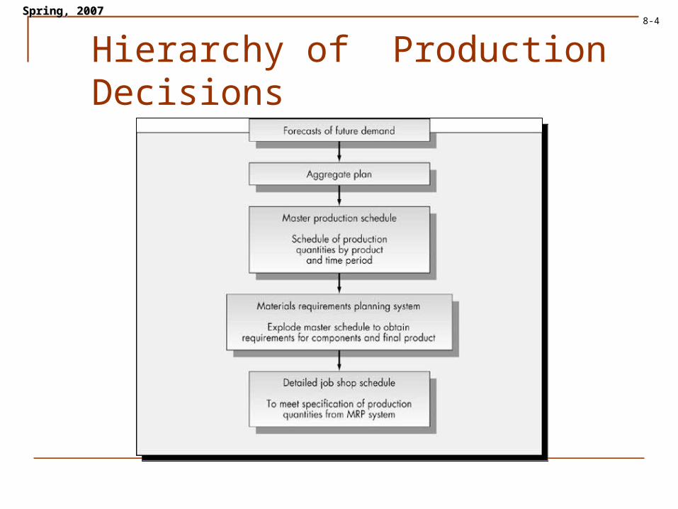
The Hierarchy of Production DecisionsThe logical sequence of operations in factory
planning corresponds to the following sequence All planning starts with the demand forecast. Demand forecasts are the basis for the top level (aggregate)
planning. The Master Production Schedule (MPS) is the result of
disaggregating aggregate plans down to the individual item level.
Based on the MPS, MRP is used to determine the size and timing of component and subassembly production.
Detailed shop floor schedules are required to meet production plans resulting from the MRP.
SpringSpring, 2007, 20078-4
Hierarchy of Production Decisions

SpringSpring, 2007, 20078-5
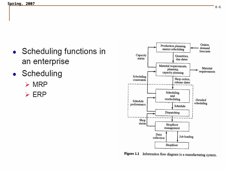
SpringSpring, 2007, 20078-6
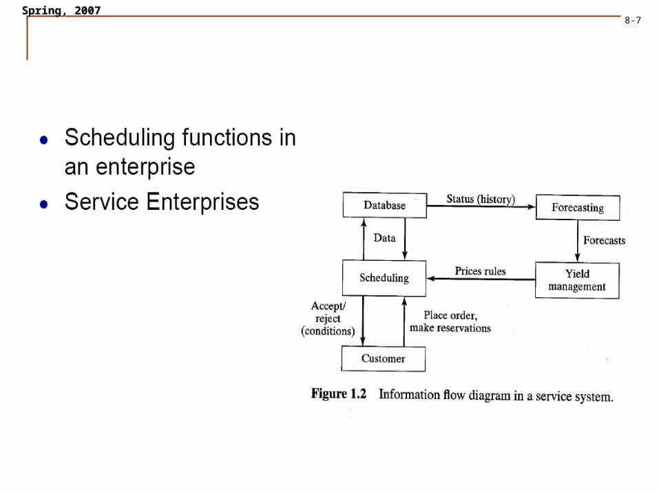
SpringSpring, 2007, 20078-7
SpringSpring, 2007, 20078-8
SpringSpring, 2007, 20078-9
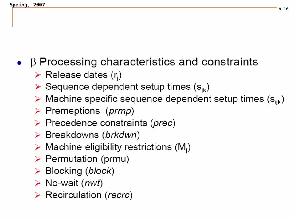
SpringSpring, 2007, 20078-10
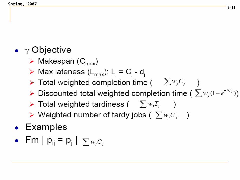
SpringSpring, 2007, 20078-11
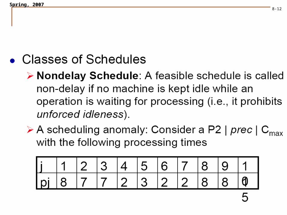
SpringSpring, 2007, 20078-12
SpringSpring, 2007, 20078-13
Characteristics of the Job Shop Scheduling Problem
Job Arrival Pattern Number and Variety of Machines Number and skill level of workers Flow Patterns Evaluation of Alternative Rules
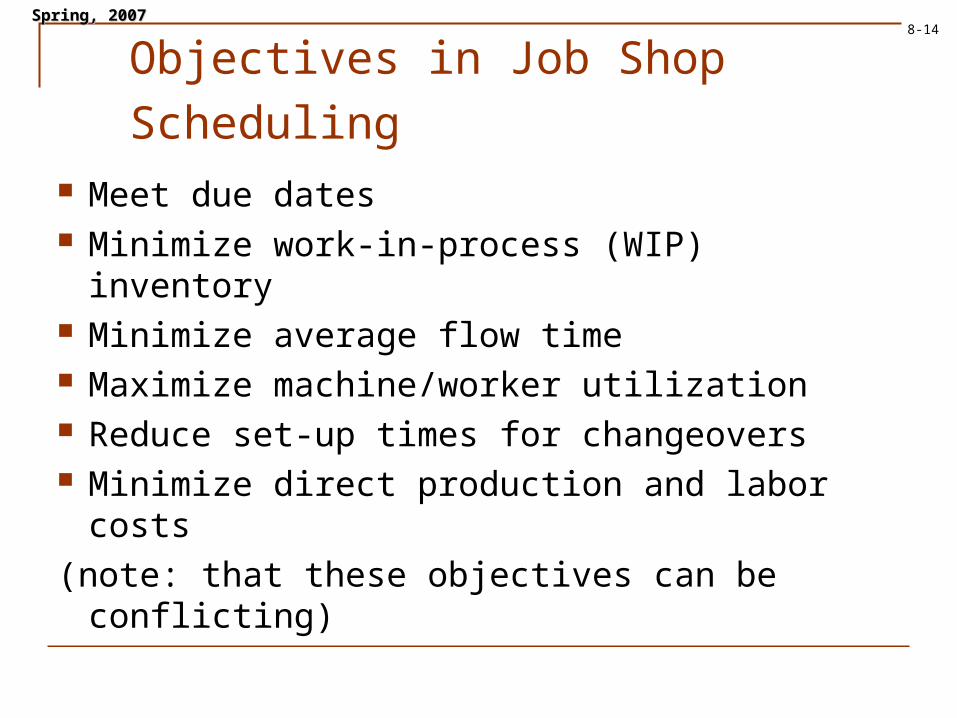
SpringSpring, 2007, 20078-14
Objectives in Job Shop Scheduling
Meet due dates Minimize work-in-process (WIP) inventory Minimize average flow time Maximize machine/worker utilization Reduce set-up times for changeovers Minimize direct production and labor costs
(note: that these objectives can be conflicting)
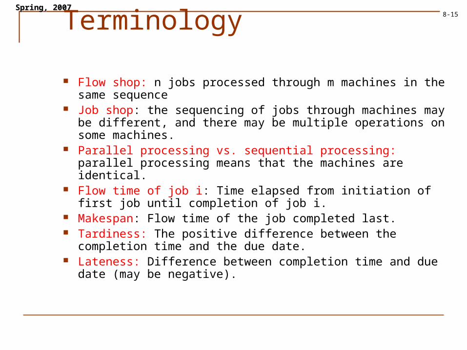
SpringSpring, 2007, 20078-15Terminology
Flow shop: n jobs processed through m machines in the same sequence
Job shop: the sequencing of jobs through machines may be different, and there may be multiple operations on some machines.
Parallel processing vs. sequential processing: parallel processing means that the machines are identical.
Flow time of job i: Time elapsed from initiation of first job until completion of job i.
Makespan: Flow time of the job completed last. Tardiness: The positive difference between the completion time
and the due date. Lateness: Difference between completion time and due date
(may be negative).
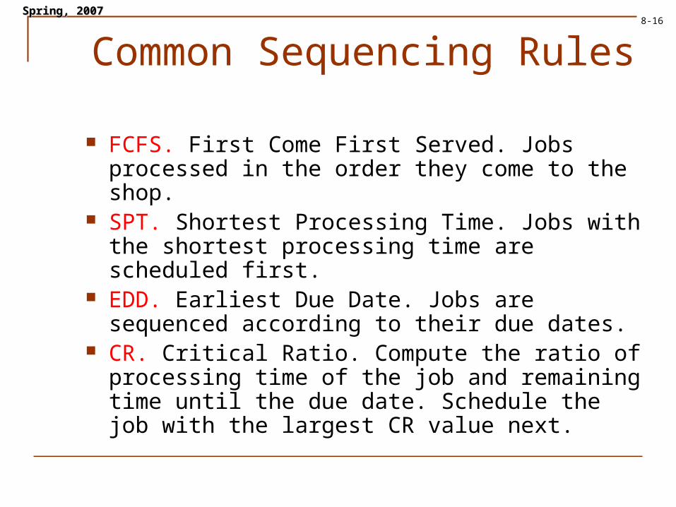
SpringSpring, 2007, 20078-16
Common Sequencing Rules
FCFS. First Come First Served. Jobs processed in the order they come to the shop.
SPT. Shortest Processing Time. Jobs with the shortest processing time are scheduled first.
EDD. Earliest Due Date. Jobs are sequenced according to their due dates.
CR. Critical Ratio. Compute the ratio of processing time of the job and remaining time until the due date. Schedule the job with the largest CR value next.

SpringSpring, 2007, 20078-17
Results for Single Machine Sequencing The rule that minimizes the mean flow time of all
jobs is SPT. The following criteria are equivalent:
Mean flow time Mean waiting time. Mean lateness
Moore’s algorithm minimizes number of tardy jobs Lawler’s algorithm minimizes the maximum flow
time subject to precedence constraints.
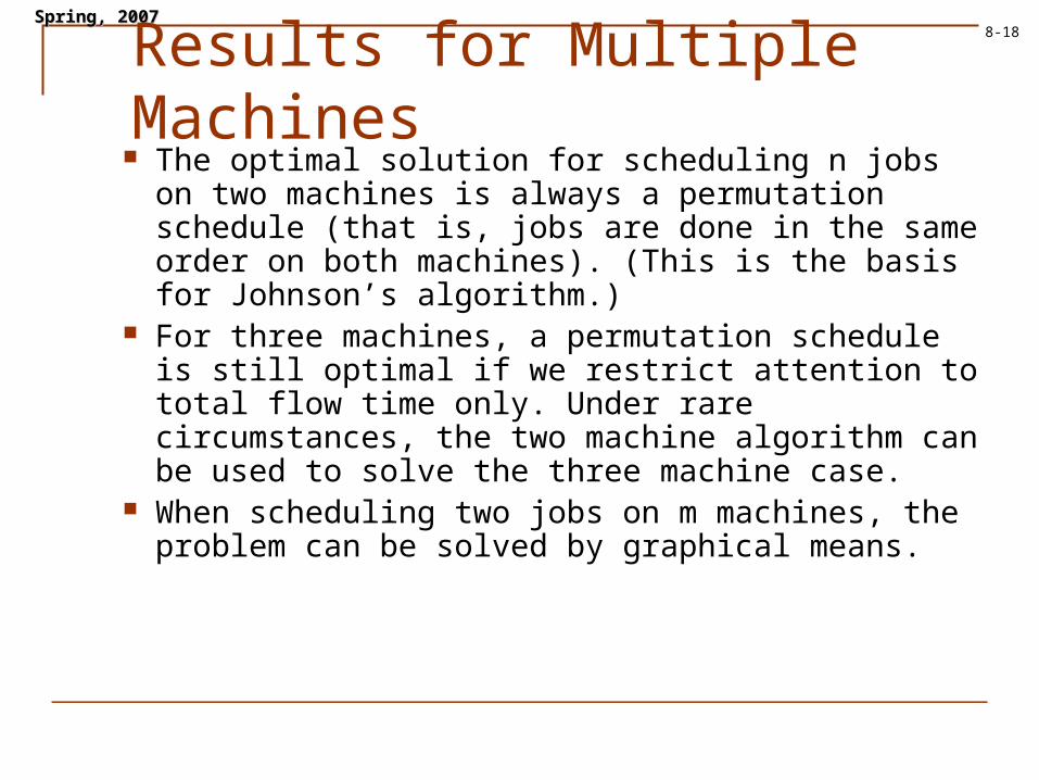
SpringSpring, 2007, 20078-18Results for Multiple
Machines The optimal solution for scheduling n jobs on two
machines is always a permutation schedule (that is, jobs are done in the same order on both machines). (This is the basis for Johnson’s algorithm.)
For three machines, a permutation schedule is still optimal if we restrict attention to total flow time only. Under rare circumstances, the two machine algorithm can be used to solve the three machine case.
When scheduling two jobs on m machines, the problem can be solved by graphical means.

SpringSpring, 2007, 20078-19
Stochastic Scheduling: Static Case Single machine case. Suppose that
processing times are random variables. If the objective is to minimize average weighted flow time, jobs are sequenced according to expected weighted SPT. That is, if job times are t1, t2, . . ., and the respective weights are u1, u2, . . . then job i precedes job i+1 if E(ti) / ui < E(ti+1) / ui+1.
SpringSpring, 2007, 20078-20
Stochastic Scheduling: Static Case (continued)
Multiple Machines. Requires the assumption that the distribution of job times is exponential, (memoryless property). Assume parallel processing of n jobs on two machines. Then the optimal sequence is to to schedule the jobs according to LEPT (longest expected processing time first).
Johnsons algorithm for scheduling n jobs on two machines in the deterministic case has a natural extension to the stochastic case as long as the job times are exponentially distributed.
SpringSpring, 2007, 20078-21
Stochastic Scheduling: Dynamic Analysis
When jobs arrive to the shop dynamically over time, queueing theory provides a means of analyzing the results. The standard M/M/1 queue applies to the case of purely random arrivals to a single machine with random processing times.
If the selection discipline does not depend on the flow times, the mean flow times are the same, but the variance of the flow times will differ.
If job times are realized when the job joins the queue rather than when the job enters service, SPT generally results in lowest expected flow time.
SpringSpring, 2007, 2007
22 of 52
8-22
Single Machine Deterministic Models
Jobs: J1, J2, ..., Jn
Assumptions:
• The machine is always available throughout the scheduling period.• The machine cannot process more than one job at a time.• Each job must spend on the machine a prescribed length of time.

SpringSpring, 2007, 20078-23
t
tJktS k
at time processed is job no if0
at time processed is job if)(
1
3
2
J1J2 J3 ...
S(t)
t
SpringSpring, 2007, 20078-24
Requirements that may restrict the feasibility of schedules:
• precedence constraints• no preemptions• release dates• deadlines
Whether some feasible schedule exist? NP hard
Objective function f is used to compare schedules.
f(S) < f(S') whenever schedule S is considered to be better than S'problem of minimising f(S) over the set of feasible schedules.

SpringSpring, 2007, 20078-25
1. Completion Time Models
Due date related objectives:
2. Lateness Models
3. Tardiness Models
4. Sequence-Dependent Setup Problems
SpringSpring, 2007, 20078-26
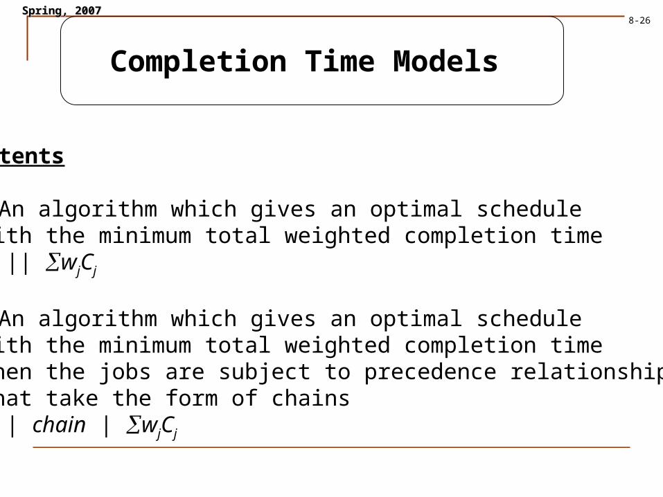
Completion Time Models
Contents
1. An algorithm which gives an optimal schedulewith the minimum total weighted completion time 1 || wjCj
2. An algorithm which gives an optimal schedule with the minimum total weighted completion time when the jobs are subject to precedence relationshipthat take the form of chains1 | chain | wjCj
SpringSpring, 2007, 20078-27
Literature:• Scheduling, Theory, Algorithms, and Systems, Michael Pinedo,
Prentice Hall, 1995, or new: Second Addition, 2002, Chapter 3.

SpringSpring, 2007, 20078-28
1 || wjCj
Theorem. The weighted shortest processing time first rule (WSPT) isoptimal for 1 || wjCj
WSPT: jobs are ordered in decreasing order of wj/pj
The next follows trivially:
The problem 1 || Cj is solved by a sequence S with jobs arranged innondecreasing order of processing times.

SpringSpring, 2007, 20078-29
Proof. By contradiction.
S is a schedule, not WSPT, that is optimal.
j and k are two adjacent jobs such that
k
k
j
j
p
w
p
w which implies that wj pk < wk pj
t t + pj + pk
j kS:
t t + pj + pk
k jS’
......
... ...
S: (t+pj) wj + (t+pj+pk) wk = t wj + pj wj + t wk + pj wk + pk wk
S’: (t+pk) wk + (t+pk+pj) wj = t wk + pk wk + t wj + pk wj + pj wj
the completion time for S’ < completion time for S contradiction!

SpringSpring, 2007, 20078-30
1 | chain | wjCj
chain 1: 1 2 ... k chain 2: k+1 k+2 ... n
Lemma. If
n
kjj
n
kjj
k
jj
k
jj
p
w
p
w
1
1
1
1
the chain of jobs 1,...,k precedes the chain of jobs k+1,...,n.
Let l* satisfy
l
jj
l
jj
kll
jj
l
jj
p
w
p
w
1
1
1*
1
*
1max
factor of chain 1,...,kl* is the job that determines the factor of the chain
SpringSpring, 2007, 20078-31
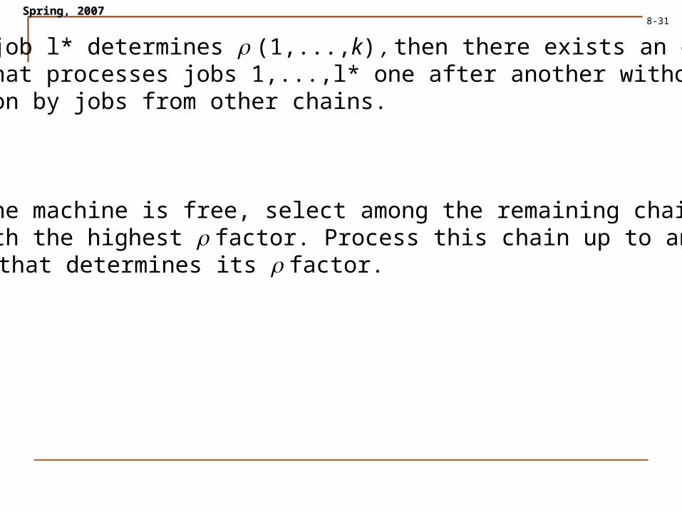
Lemma. If job l* determines (1,...,k) , then there exists an optimalsequence that processes jobs 1,...,l* one after another withoutinterruption by jobs from other chains.
Algorithm
Whenever the machine is free, select among the remaining chainsthe one with the highest factor. Process this chain up to and includingthe job l* that determines its factor.
SpringSpring, 2007, 20078-32
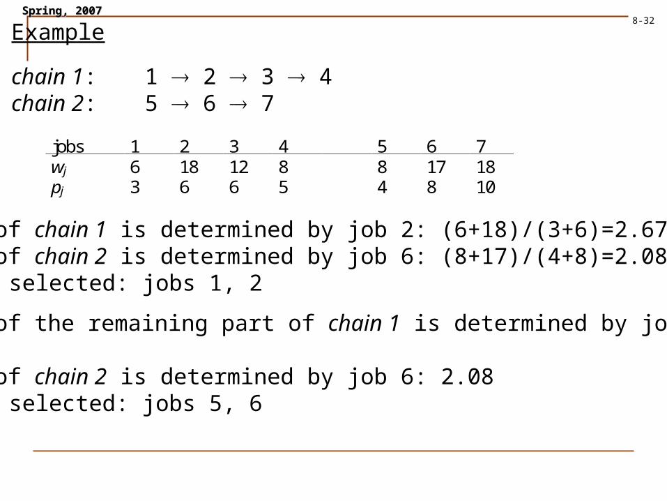
Example
chain 1: 1 2 3 4chain 2: 5 6 7
jobs 1 2 3 4 5 6 7wj 6 18 12 8 8 17 18pj 3 6 6 5 4 8 10
factor of chain 1 is determined by job 2: (6+18)/(3+6)=2.67 factor of chain 2 is determined by job 6: (8+17)/(4+8)=2.08chain 1 is selected: jobs 1, 2
factor of the remaining part of chain 1 is determined by job 3:12/6=2 factor of chain 2 is determined by job 6: 2.08chain 2 is selected: jobs 5, 6
SpringSpring, 2007, 20078-33
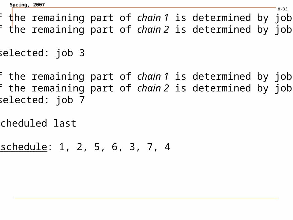
factor of the remaining part of chain 1 is determined by job 3: 2 factor of the remaining part of chain 2 is determined by job 7:18/10=1.8chain 1 is selected: job 3
factor of the remaining part of chain 1 is determined by job 4: 8/5=1.6 factor of the remaining part of chain 2 is determined by job 7: 1.8chain 2 is selected: job 7
job 4 is scheduled last
the final schedule: 1, 2, 5, 6, 3, 7, 4

SpringSpring, 2007, 20078-34
1 | prec | wjCj
Polynomial time algorithms for the more complex precedenceconstraints than the simple chains are developed.
The problems with arbitrary precedence relation are NP hard.
1 | rj, prmp | wjCj preemptive version of the WSPT ruledoes not always lead to an optimal solution,the problem is NP hard
1 | rj, prmp | Cj preemptive version of the SPT rule is optimal
1 | rj | Cj is NP hard
SpringSpring, 2007, 20078-35
Summary
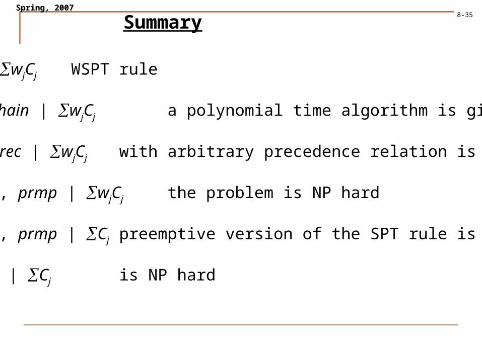
1 || wjCj WSPT rule
1 | chain | wjCj a polynomial time algorithm is given
1 | prec | wjCj with arbitrary precedence relation is NP hard
1 | rj, prmp | wjCjthe problem is NP hard
1 | rj, prmp | Cj preemptive version of the SPT rule is optimal
1 | rj | Cj is NP hard
SpringSpring, 2007, 2007
36 of 52
8-36
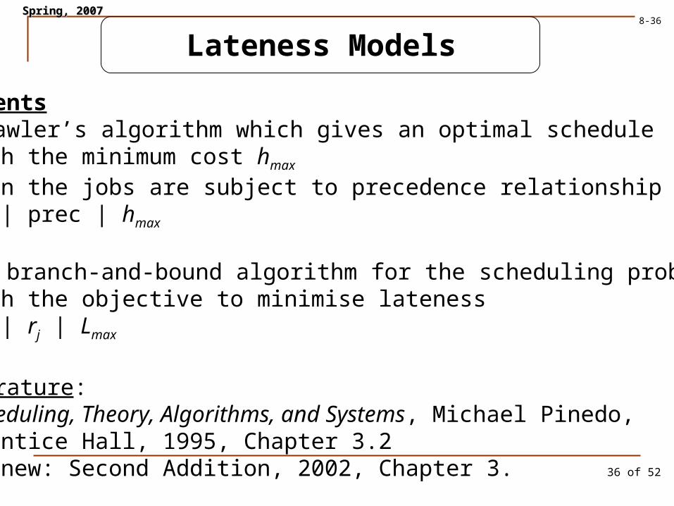
Lateness Models
Contents1. Lawler’s algorithm which gives an optimal schedule
with the minimum cost hmax
when the jobs are subject to precedence relationship 1 | prec | hmax
2. A branch-and-bound algorithm for the scheduling problemswith the objective to minimise lateness 1 | rj | Lmax
Literature:• Scheduling, Theory, Algorithms, and Systems, Michael Pinedo,
Prentice Hall, 1995, Chapter 3.2or new: Second Addition, 2002, Chapter 3.
SpringSpring, 2007, 20078-37
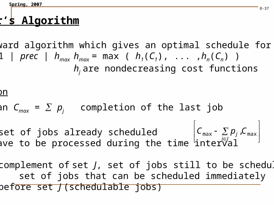
Lawler’s Algorithm
• Backward algorithm which gives an optimal schedule for1 | prec | hmax hmax = max ( h1(C1), ... ,hn(Cn) )
hj are nondecreasing cost functions
Notation
makespan Cmax = pj completion of the last job
J set of jobs already scheduledthey have to be processed during the time interval
JC complement of set J, set of jobs still to be scheduledJ' JC set of jobs that can be scheduled immediately
before set J (schedulable jobs)
Jjj CpC maxmax ,
SpringSpring, 2007, 20078-38
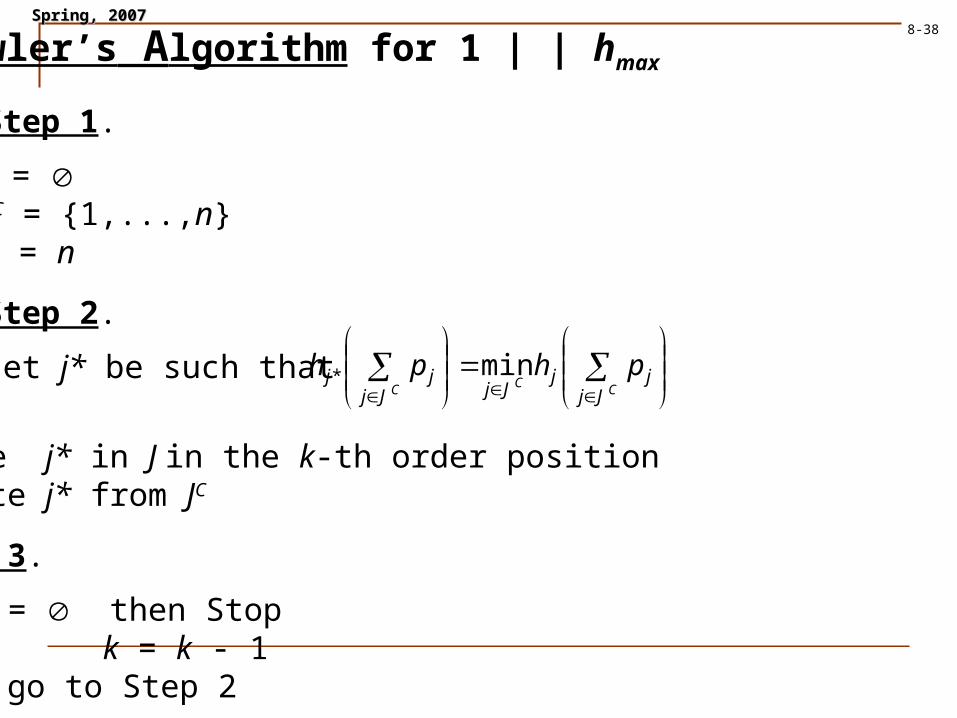
Step 1.
J = JC = {1,...,n}k = n
Step 2.
Let j* be such that
CCC Jj
jjJjJj
jj phph min*
Place j* in J in the k-th order positionDelete j* from JC
Step 3.
If JC = then Stopelse k = k - 1
go to Step 2
Lawler’s Algorithm for 1 | | hmax
SpringSpring, 2007, 20078-39
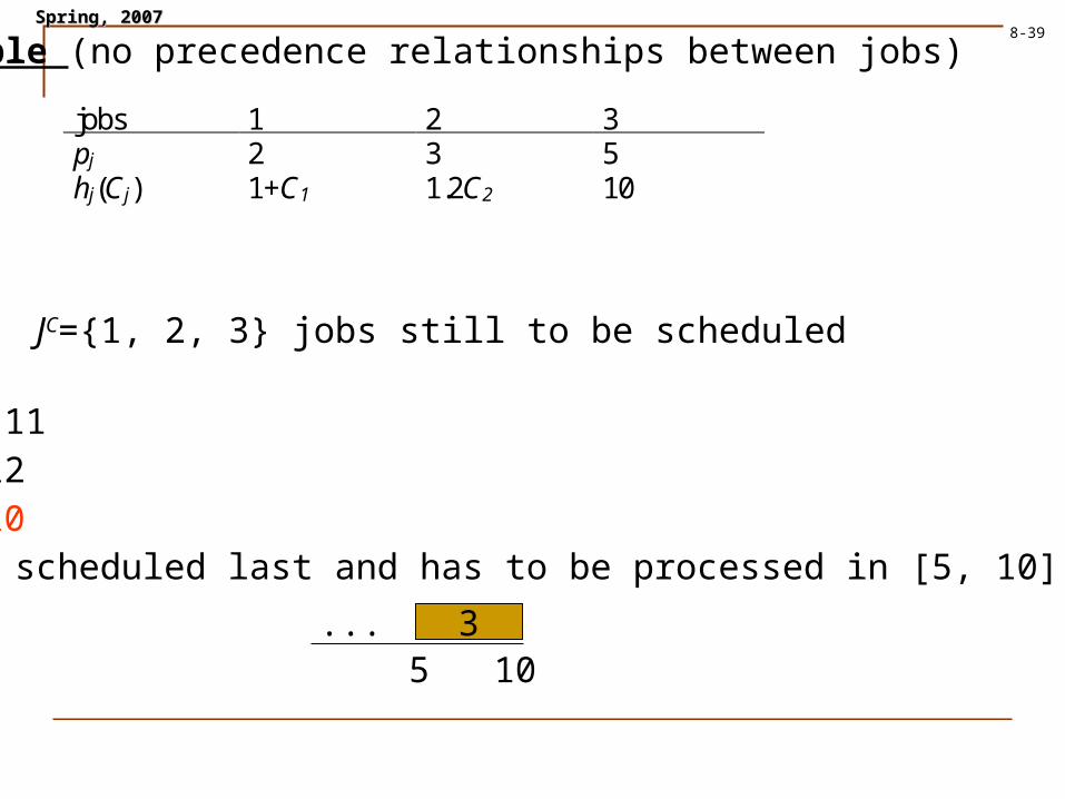
Example (no precedence relationships between jobs)
jobs 1 2 3pj 2 3 5hj(Cj) 1+C1 1.2C2 10
J = JC={1, 2, 3} jobs still to be scheduledCmax = 10h1(10) = 11h2(10) =12h3(10) =10 Job 3 is scheduled last and has to be processed in [5, 10].
105... 3

SpringSpring, 2007, 20078-40
J = {3} JC={1, 2} jobs still to be scheduledCmax = 5h1(5) = 6h2(5) = 6Either job 1 or job 2 may be processed before job 3.
105321
105312
or
Two schedules are optimal: 1, 2, 3 and 2, 1, 3
SpringSpring, 2007, 20078-41
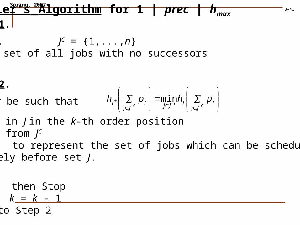
Step 1.
J = , JC = {1,...,n}J' the set of all jobs with no successorsk = n
Step 2.
Let j* be such that
CC Jj
jjJjJj
jj phph'
* min
Place j* in J in the k-th order position Delete j* from JC
Modify J' to represent the set of jobs which can be scheduledimmediately before set J.Step 3.
If JC = then Stopelse k = k - 1
go to Step 2
Lawler’s Algorithm for 1 | prec | hmax
SpringSpring, 2007, 20078-42
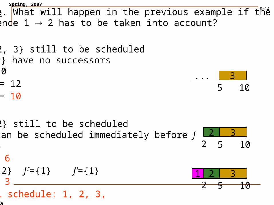
Example. What will happen in the previous example if theprecedence 1 2 has to be taken into account?
J = JC={1, 2, 3} still to be scheduled J'={2, 3} have no successorsCmax = 10h2(10) = 12h3(10) = 10
J = {3}JC={1, 2} still to be scheduled J'={2} can be scheduled immediately before J Cmax = 5h2(5) = 6J = {3, 2} JC={1} J'={1} h1(2) = 3Optimal schedule: 1, 2, 3,hmax = 10
105... 3
105321
10532
2
2
SpringSpring, 2007, 20078-43
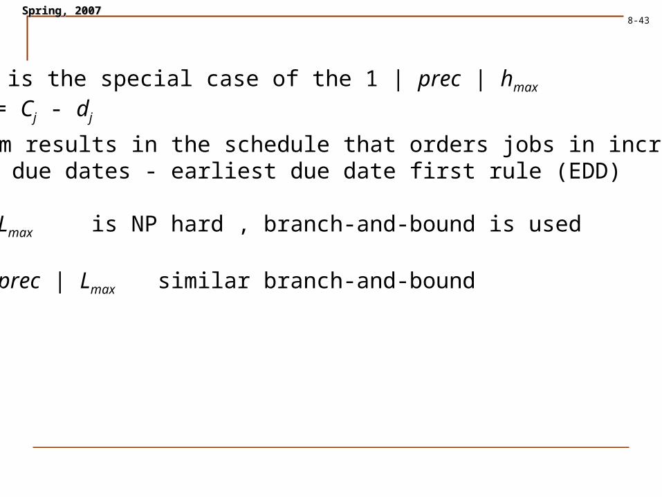
1 || Lmax is the special case of the 1 | prec | hmax
where hj = Cj - dj
algorithm results in the schedule that orders jobs in increasing orderof their due dates - earliest due date first rule (EDD)
1 | rj | Lmax is NP hard , branch-and-bound is used
1 | rj , prec | Lmax similar branch-and-bound
SpringSpring, 2007, 20078-44
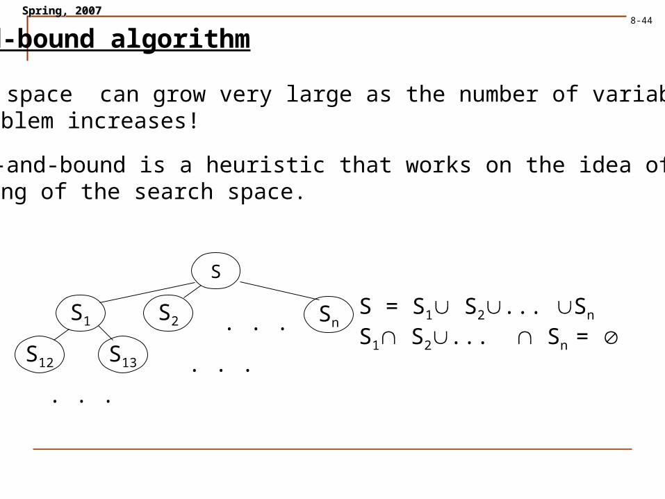
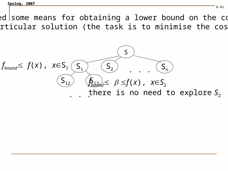
Branch-and-bound algorithm
• Search space can grow very large as the number of variablesin the problem increases!
• Branch-and-bound is a heuristic that works on the idea of successivepartitioning of the search space.
S
S1 S2 Sn
S12 S13
. . .
. . .
. . .
S = S1 S2... Sn
S1 S2... Sn =
SpringSpring, 2007, 20078-45
S
S1 S2 Sn
S12 S13
. . .
. . .
• We need some means for obtaining a lower bound on the cost forany particular solution (the task is to minimise the cost).
fbound f(x), xS1
fbound f(x), xS2
there is no need to explore S2

SpringSpring, 2007, 20078-46
Branch-and-bound algorithm
Step 1Initialise P = Si (determine the partitions)Initialise fbound
Step 2Remove best partition Si from PReduce or subdivide Si into Sij
Update fbound
P = P Sij
For all SijP doif lower bound of f(Sij) > fbound then remove Sij from P
Step 3If not termination condition then go to Step 2
SpringSpring, 2007, 20078-47
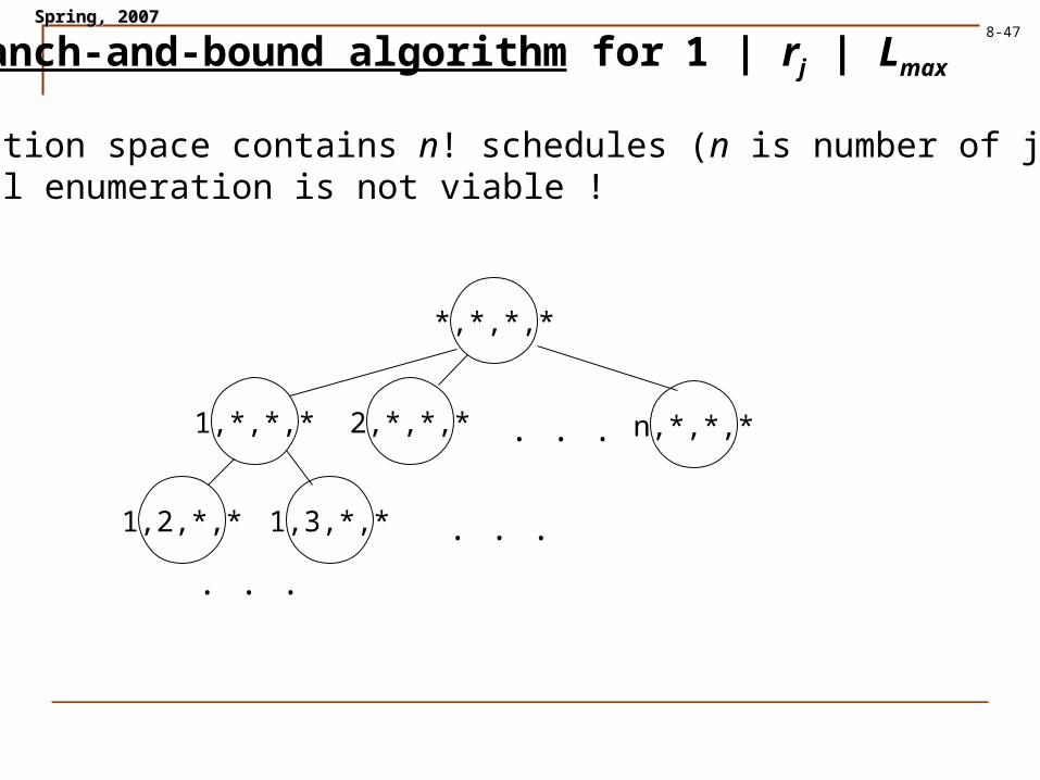
*,*,*,*
1,*,*,* 2,*,*,* n,*,*,*
1,2,*,* 1,3,*,*
. . .
. . .
. . .
Branch-and-bound algorithm for 1 | rj | Lmax
Solution space contains n! schedules (n is number of jobs).Total enumeration is not viable !
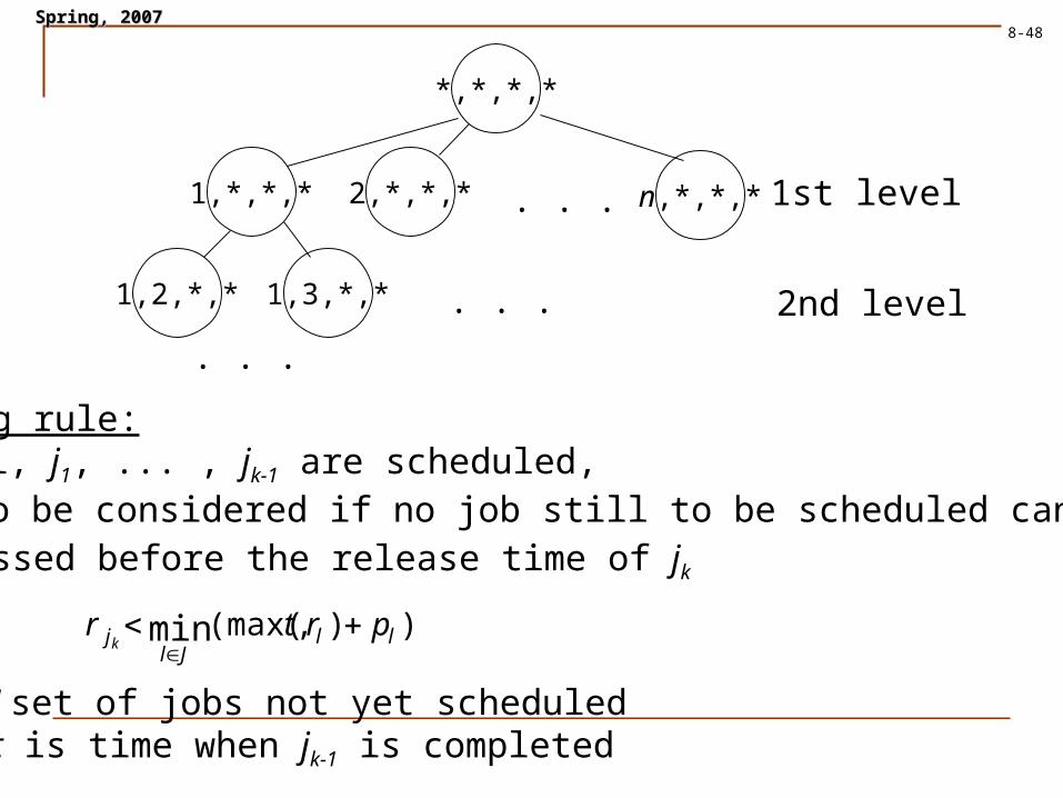
SpringSpring, 2007, 20078-48
Branching rule:k-1 level, j1, ... , jk-1 are scheduled,jk need to be considered if no job still to be scheduled can notbe processed before the release time of jk that is: )),(max(min ll
Jlj prtrk
J set of jobs not yet scheduledt is time when jk-1 is completed
*,*,*,*
1,*,*,* 2,*,*,* n,*,*,*
1,2,*,* 1,3,*,*
. . .
. . .
. . .
1st level
2nd level

SpringSpring, 2007, 20078-49
Lower bound:
• Preemptive earliest due date (EDD) rule is optimal for 1 | rj prmp | Lmax
A preemptive schedule will have a maximum latenessnot greater than a non-preemtive schedule.
• If a preemptive EDD rule gives a nonpreemptive schedule thenall nodes with a larger lower bound can be disregarded.
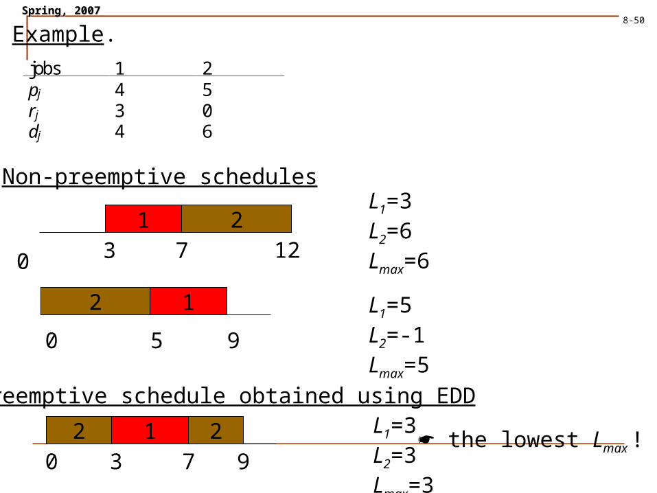
SpringSpring, 2007, 20078-50
Example.jobs 1 2pj 4 5rj 3 0dj 4 6
• Non-preemptive schedules
0
1 2
3 7 12
2 1
0 5 9
L1=3L2=6Lmax=6
L1=5L2=-1Lmax=5
• Preemptive schedule obtained using EDD
2 1 2
0 3 7 9
L1=3L2=3Lmax=3
the lowest Lmax !

SpringSpring, 2007, 20078-51
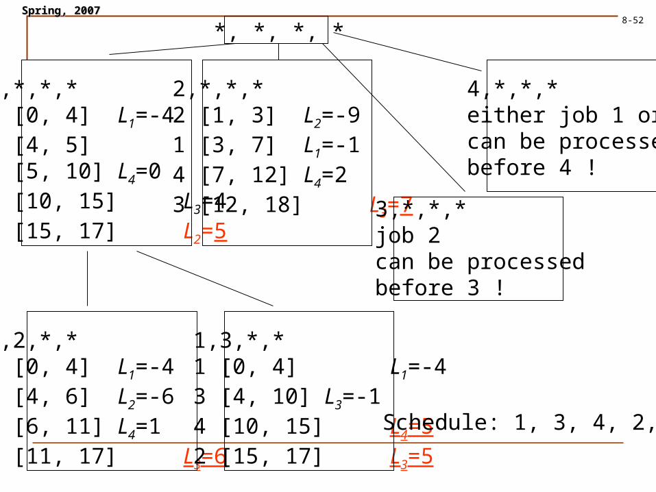
Example
jobs 1 2 3 4pj 4 2 6 5rj 0 1 3 5dj 8 12 11 10
*,*,*,*
1,*,*,* 2,*,*,* 4,*,*,*
1,2,*,* 1,3,*,*
3,*,*,*
job 2 could be processedbefore job 3
job 1 could be processedbefore job 4
1,3,4,2
L.B. = 5 L.B. = 7
L.B. = 6L.B. = 5
SpringSpring, 2007, 20078-52
*, *, *, *
1,*,*,*1 [0, 4] L1=-43 [4, 5]4 [5, 10] L4=03 [10, 15] L3=42 [15, 17] L2=5
2,*,*,*2 [1, 3] L2=-91 [3, 7] L1=-14 [7, 12] L4=23 [12, 18] L3=7
1,2,*,*1 [0, 4] L1=-42 [4, 6] L2=-64 [6, 11] L4=13 [11, 17] L3=6
1,3,*,*1 [0, 4] L1=-43 [4, 10] L3=-14 [10, 15] L4=52 [15, 17] L3=5
Schedule: 1, 3, 4, 2,
4,*,*,*either job 1 or 2can be processedbefore 4 !
3,*,*,*job 2can be processedbefore 3 !

SpringSpring, 2007, 20078-53
Summary
1 | prec | hmax , hmax=max( h1(C1), ... ,hn(Cn) ), Lawler’s algorithm
1 || Lmax EDD rule
1 | rj | Lmax is NP hard , branch-and-bound is used
1 | rj , prec | Lmax similar branch-and-bound
1 | rj, prmp | Lmax preemptive EDD rule
SpringSpring, 2007, 2007
54 of 52
8-54
Tardiness Models
Contents
1. Moor’s algorithm which gives an optimal schedulewith the minimum number of tardy jobs 1 || Uj
2. An algorithm which gives an optimal schedule with the minimum total tardiness 1 || Tj
Literature:• Scheduling, Theory, Algorithms, and Systems, Michael Pinedo,
Prentice Hall, 1995, Chapters 3.3 and 3.4or new: Second Addition, 2002, Chapter 3.
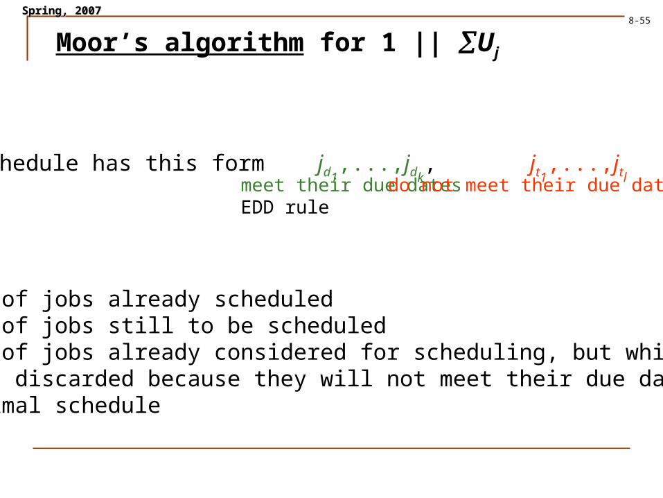
SpringSpring, 2007, 20078-55
Optimal schedule has this form jd1,...,jdk
, jt1,...,jtl
NotationJ set of jobs already scheduledJC set of jobs still to be scheduledJd set of jobs already considered for scheduling, but which have
been discarded because they will not meet their due date in theoptimal schedule
meet their due datesEDD rule
do not meet their due dates
Moor’s algorithm for 1 || Uj
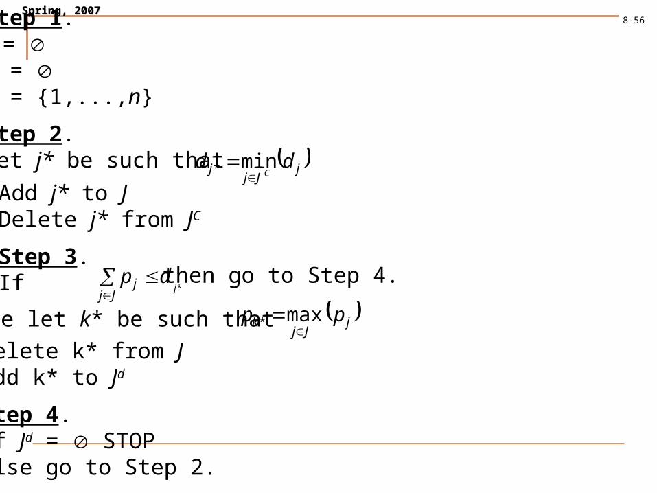
SpringSpring, 2007, 20078-56Step 1.
J = Jd = JC = {1,...,n}
Step 2.Let j* be such that j
Jjj dd
Cmin*
Add j* to JDelete j* from JC
Step 3.If *j
dpJj
j
else let k* be such that jJj
k pp
max*
Delete k* from JAdd k* to Jd
Step 4.If Jd = STOPelse go to Step 2.
then go to Step 4.
SpringSpring, 2007, 20078-57
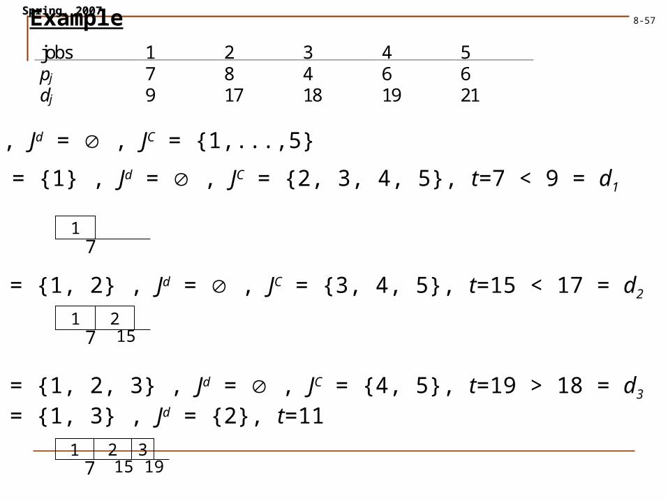
jobs 1 2 3 4 5pj 7 8 4 6 6dj 9 17 18 19 21
Example
J = , Jd = , JC = {1,...,5}
j*=1 J = {1} , Jd = , JC = {2, 3, 4, 5}, t=7 < 9 = d1
71
71 2
15
71 2
15319
j*=2 J = {1, 2} , Jd = , JC = {3, 4, 5}, t=15 < 17 = d2
j*=3 J = {1, 2, 3} , Jd = , JC = {4, 5}, t=19 > 18 = d3
k*=2 J = {1, 3} , Jd = {2}, t=11

SpringSpring, 2007, 20078-58
j*=4 J = {1, 3, 4} , Jd = {2}, JC = {5}, t=17 < 19 = d4
j*=5 J = {1, 3, 4, 5} , Jd = {2}, JC = , t=23 > 21 = d5
k*=1 J = {3, 4, 5} , Jd = {2, 1}, t=16 < 21 = d5
optimal schedule 3, 4, 5, 1, 2 Uj = 2
71 3
154
17
71 3
154
175
23
SpringSpring, 2007, 20078-59
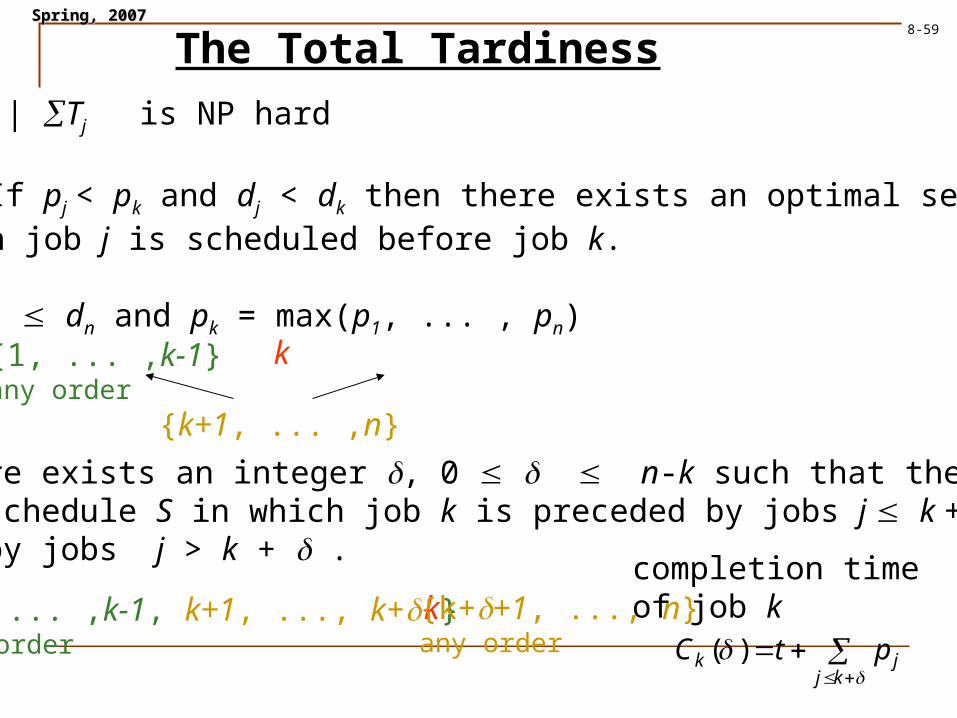
The Total Tardiness
1 || Tj is NP hard
Lemma. If pj < pk and dj < dk then there exists an optimal sequencein which job j is scheduled before job k.
d1 ... dn and pk = max(p1, ... , pn){1, ... ,k-1}any order
k
{k+1, ... ,n}
Lemma.There exists an integer , 0 n-k such that there is anoptimal schedule S in which job k is preceded by jobs j k + andfollowed by jobs j > k + .
k{1, ... ,k-1, k+1, ..., k+ }any order
{k++1, ..., n}any order
kjjk ptC )(
completion timeof job k

SpringSpring, 2007, 20078-60
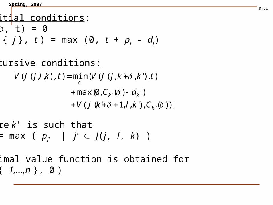
PRINCIPLE OF OPTIMALITY, Bellman 1956. An optimal policy has the property that whatever the initial state andthe initial decision are, the remaining decisions must constitute anoptimal policy with regard to the state resulting from the firstdecision.
Algorithm
Dynamic programming procedure: recursively the optimal solution forsome job set J starting at time t is determined from the optimal solutionsto subproblems defined by job subsets of S*S with start times t*t .
J(j, l, k) contains all the jobs in a set {j, j+1, ... , l} with processing time pk
V( J(j, l, k) , t) total tardiness of the subset under an optimal sequenceif this subset starts at time t
SpringSpring, 2007, 20078-61
Initial conditions:V(, t) = 0V( { j }, t ) = max (0, t + pj - dj)
Recursive conditions:
)))(,)',,1'((
))(,0max(
),)',',(((min),),,((
'
''
k
kk
CklkJV
dC
tkkjJVtkljJV
where k' is such thatpk' = max ( pj' | j' J(j, l, k) )
Optimal value function is obtained forV( { 1,...,n }, 0 )
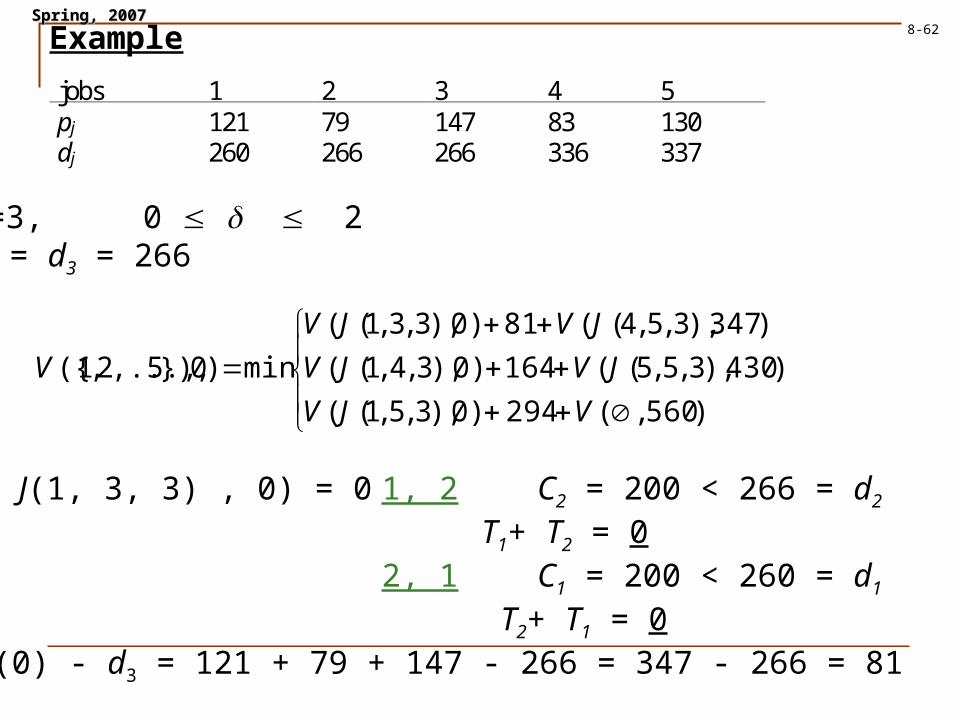
SpringSpring, 2007, 20078-62Example
jobs 1 2 3 4 5pj 121 79 147 83 130dj 260 266 266 336 337
k'=3, 0 2 dk' = d3 = 266
)560,(294)0),3,5,1((
)430),3,5,5((164)0),3,4,1((
)347),3,5,4((81)0),3,3,1((
min)0}),5,...,2,1({
VJV
JVJV
JVJV
V
V( J(1, 3, 3) , 0) = 0 1, 2 C2 = 200 < 266 = d2
T1+ T2 = 02, 1 C1 = 200 < 260 = d1
T2+ T1 = 0C3(0) - d3 = 121 + 79 + 147 - 266 = 347 - 266 = 81
SpringSpring, 2007, 20078-63
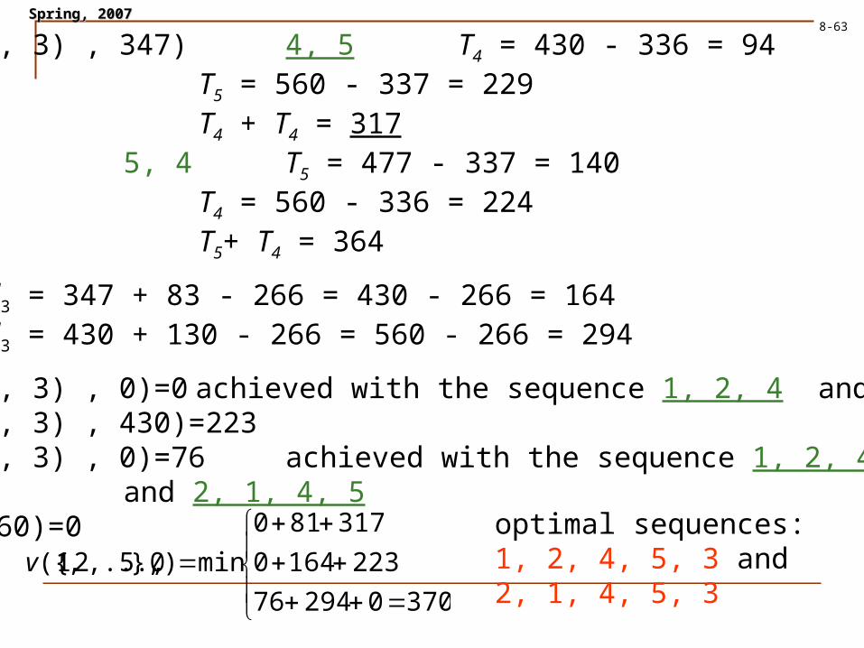
V( J(4, 5, 3) , 347) 4, 5 T4 = 430 - 336 = 94T5 = 560 - 337 = 229
T4 + T4 = 3175, 4 T5 = 477 - 337 = 140
T4 = 560 - 336 = 224 T5+ T4 = 364
C3(1) - d3 = 347 + 83 - 266 = 430 - 266 = 164C3(2) - d3 = 430 + 130 - 266 = 560 - 266 = 294
V( J(1, 4, 3) , 0)=0 achieved with the sequence 1, 2, 4 and 2, 1, 4V( J(5, 5, 3) , 430)=223V( J(1, 5, 3) , 0)=76 achieved with the sequence 1, 2, 4, 5
and 2, 1, 4, 5 V( , 560)=0
370029476
2231640
317810
min)0},5,...,2,1({v
optimal sequences:1, 2, 4, 5, 3 and2, 1, 4, 5, 3
SpringSpring, 2007, 20078-64
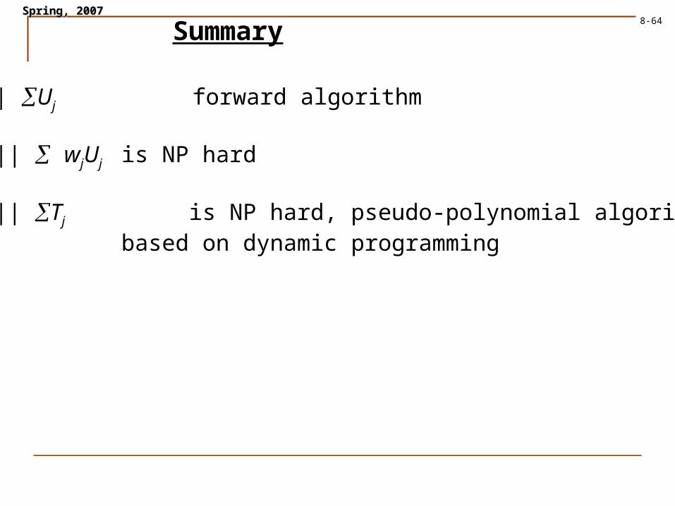
Summary
1 || Uj forward algorithm
1 || wjUj is NP hard
1 || Tj is NP hard, pseudo-polynomial algorithmbased on dynamic programming

SpringSpring, 2007, 20078-65
Assembly Line Balancing
Characteristics of the Assembly Line Balancing problem. A collection of n tasks must be completed on each item Tasks are assigned to stations. Tasks must be sequenced
properly, and certain tasks may not be done at the same station.
The objective is to assign tasks to stations to minimize the cycle time, C.
The general problem is difficult to solve optimally, but effective heuristics are available. (the text discusses one known as the ranked positional weight technique.)
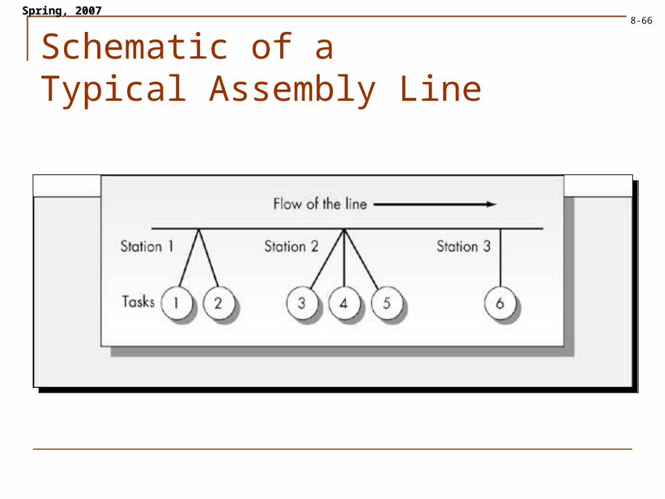
SpringSpring, 2007, 20078-66
Schematic of a Typical Assembly Line