Embed Size (px)
Citation preview

JOBS WORKING
PAPERIssue No. 60
How Did the COVID-19 Crisis Affect Different Types of Workers
in the Developing World?
Maurice Kugler, Mariana Viollaz, Daniel Duque,Isis Gaddis, David Newhouse, Amparo Palacios-Lopez,
and Michael Weber
Pub
lic D
iscl
osur
e A
utho
rized
Pub
lic D
iscl
osur
e A
utho
rized
Pub
lic D
iscl
osur
e A
utho
rized
Pub
lic D
iscl
osur
e A
utho
rized

HOW DID THE COVID-19 CRISIS AFFECT DIFFERENT TYPES OF WORKERS IN THE
DEVELOPING WORLD?
Maurice Kugler, Mariana Viollaz, Daniel Duque,
Isis Gaddis, David Newhouse, Amparo Palacios-Lopez, and Michael Weber

© 2021 International Bank for Reconstruction and Development / The World Bank.
1818 H Street NW, Washington, DC 20433, USA.
Telephone: 202-473-1000; Internet: www.worldbank.org.
Some rights reserved
This work is a product of the staff of The World Bank with external contributions. The findings, interpretations, and
conclusions expressed in this work do not necessarily reflect the views of The World Bank, its Board of Executive
Directors, or the governments they represent. The World Bank does not guarantee the accuracy of the data
included in this work. The boundaries, colors, denominations, and other information shown on any map in this
work do not imply any judgment on the part of The World Bank concerning the legal status of any territory or the
endorsement or acceptance of such boundaries.
Nothing herein shall constitute or be considered to be a limitation upon or waiver of the privileges and immunities
of The World Bank, all of which are specifically reserved.
Rights and Permissions
This work is available under the Creative Commons Attribution 3.0 IGO license (CC BY 3.0 IGO)
http://creativecommons.org/licenses/by/3.0/igo. Under the Creative Commons Attribution license, you are free to
copy, distribute, transmit, and adapt this work, including for commercial purposes, under the following conditions:
Attribution—Please cite the work as follows: Kugler, M. Mariana Viollaz, Daniel Duque, Isis Gaddis, David
Newhouse, Amparo Palacios-Lopez, and Michael Weber et al. 2021. “How Did the COVID-19 Crisis Affect Different
Types of Workers in The Developing World?” World Bank, Washington, DC. License: Creative Commons Attribution
CC BY 3.0 IGO.
Translations—If you create a translation of this work, please add the following disclaimer along with the
attribution: This translation was not created by The World Bank and should not be considered an official World
Bank translation. The World Bank shall not be liable for any content or error in this translation.
Adaptations—If you create an adaptation of this work, please add the following disclaimer along with the
attribution: This is an adaptation of an original work by The World Bank. Views and opinions expressed in the
adaptation are the sole responsibility of the author or authors of the adaptation and are not endorsed by The
World Bank.
Third-party content—The World Bank does not necessarily own each component of the content contained within
the work. The World Bank therefore does not warrant that the use of any third-party-owned individual component
or part contained in the work will not infringe on the rights of those third parties. The risk of claims resulting from
such infringement rests solely with you. If you wish to re-use a component of the work, it is your responsibility to
determine whether permission is needed for that re-use and to obtain permission from the copyright owner.
Examples of components can include, but are not limited to, tables, figures, or images.
All queries on rights and licenses should be addressed to World Bank Publications, The World Bank Group,
1818 H Street NW, Washington, DC 20433, USA; fax: 202-522-2625; e-mail: [email protected].
How Did the COVID-19 Crisis Affect Different Types of
Workers in the Developing World?
June 2021
Maurice Kugler*
Mariana Viollaz†
Daniel Duque‡
Isis Gaddis§
David Newhouse§
Amparo Palacios-Lopez§
Michael Weber§
Abstract This paper investigates the impacts of the economic shock caused by the COVID-19 pandemic on
the employment of different types of workers in developing countries. Employment outcomes are
taken from a set of high-frequency phone surveys conducted by the World Bank and National
Statistics Offices in 40 countries. Larger shares of female, young, less educated, and urban workers
stopped working. Gender gaps in work stoppage were particularly pronounced and stemmed
mainly from differences within sectors rather than differential employment patterns across sectors.
Differences in work stoppage between urban and rural workers were markedly smaller than those
across gender, age, and education groups. Preliminary results from 10 countries suggest that
following the initial shock at the start of the pandemic, employment rates partially recovered
between April and August, with greater gains for those groups that had borne the brunt of the early
jobs losses. Although the high-frequency phone surveys greatly over-represent household heads
and therefore overestimate employment rates, case studies in five countries suggest that they
provide a reasonably accurate measure of disparities in employment levels by gender, education,
and urban/rural location following the onset of the crisis, although they perform less well in
capturing disparities between age groups. These results shed new light on the labor market
consequences of the COVID-19 crisis in developing countries, and suggest that real-time phone
surveys, despite their lack of representativeness, are a valuable source of information to measure
differential employment impacts across groups during a crisis.
Keywords: COVID-19, pandemic shock, unemployment, worker displacement, coping
mechanisms, post-shock differential employment evolution, heterogenous labor market impacts,
high-frequency phone surveys
* Schar School of Policy and Government, George Mason University † CEDLAS ‡ Norwegian School of Economics § World Bank Group

JEL Codes: E24, J15, J16, J21
Acknowledgements: We gratefully acknowledge funding from the Jobswatch Covid-19 project.
We thank Benu Bidani, Kathleen Beegle, Wendy Cunningham, Ambar Narayan, Ian Walker, and
World Bank seminar participants for helpful comments. We thank Nobuo Yoshida for providing
the harmonized high-frequency phone survey data, and Ivette Maria Contreras Gonzalez for
providing survey data from Malawi and Nigeria. We thank Benu Bidani, Gero Carletto, Caren
Grown, Michal Rutkowski, Carolina Sanchez-Paramo, and Ian Walker for their support.

1. Introduction
The 2020-21 COVID-19 crisis represented an unprecedented and massive shock to labor markets
worldwide. Yet there is very little systematic documented evidence about the crisis’s impact on
different types of workers in developing countries. Empirical evidence from developed countries
suggests that traditionally disadvantaged workers in the labor market were disproportionately
affected by the pandemic (Lee et al., 2021; Fairlie et al., 2020). These studies document that
inequality has been exacerbated by utilizing a variety of data sources to explore the labor market
impacts of the pandemic, such as government administrative data, real-time surveys, and
information from social media. Much less is known about the impacts of the shock on workers in
developing countries, since the pandemic disrupted traditional data collection systems in many of
these countries and alternative data sources are rarely available.
This study draws on information from a set of High Frequency Phone Surveys (HFPS), collected
and harmonized by the World Bank for 40 countries, to explore which types of workers in
developing countries were hit hardest by the labor market impacts of COVID-19. A companion
paper to the current analysis by Khamis et al. (2021) already quantifies the massive early adverse
labor market impacts of COVID-19 in developing countries using the HFPS data. This paper
focuses on the distributional implications of the crisis, in order to shed light on the extent to which
the crisis is exacerbating traditional disparities and the potential need for policy interventions.
The HFPS have the virtue of collecting data widely and fast. However, they are potentially subject
to sampling and selection biases that are crucial to consider carefully. The HFPS can provide a
biased picture of employment changes during the COVID-19 pandemic for two reasons. First, only
households where at least one member had a phone, access to electricity, and were willing to
participate in the survey were interviewed. This will lead to bias if people who were not
represented in the sample experienced systematically different labor market outcomes than those
who were represented. Second, in many countries the samples overrepresent household heads and
underrepresent children and other non-spouse household members, affecting the
representativeness of the survey at the individual level in the selection of the sample and providing
a biased picture of labor market outcomes. Phone surveys drawn from an existing sample were
more likely to overrepresent the household head than phone surveys that used a different sampling
approach (mostly Random Digit Dialing), because the recontact information was captured only or

mainly for the head of household. In addition, the household head was also interviewed in contexts
where it was difficult to contact other household members without the head’s authorization, in
order to reduce non-response. Finally, some surveys elected to collect information on the head
under the assumption that they are the main income earner in the household.
In 19 of the 40 countries included in this study, the sample was drawn from a previous survey. In
these cases, household weights were constructed by World Bank country teams in conjunction
with national statistics offices, often by using information from prior surveys on phone ownership
and other household characteristics. Evidence from four African countries suggests that this
reweighting procedure was highly effective at reducing bias among sample households (Ambel et
al, 2021). In contrast, the second source of bias, individual sampling bias, was not addressed by
the teams producing the data. Evidence from the same four African countries indicates that this
leads to overrepresentation of heads, as well as respondents who were older, more educated, and
own a household enterprise. Furthermore, there is evidence that reweighting using an individual-
level model is only partially able to address the sample selection bias that arises from the non-
random selection of individuals (Brubaker et al, 2021).
While the main objective of the paper is to document differential employment impacts of the
COVID-19 pandemic across groups, it is important to test the extent to which sample selection
bias may affect comparisons of individual labor market outcomes to be confident in the results.
We examine the role of sample selection bias in two ways. First, in an exercise similar to that
carried out by Brubaker et al (2021), we reweight observations in the HFPS based on individual
characteristics to match nationally representative microdata collected prior to the pandemic.
Second, we evaluate the performance of standard estimates that use the household weights
calculated by the World Bank teams, as well as the reweighted estimates based on individual
characteristics, in five countries. These five countries are unusual because they collected survey
data during the pandemic that contains information on the labor market outcomes of all household
members, which provides a natural benchmark for evaluating the extent of the individual sampling
bias in the HFPS data.
This paper has five key findings:
1. Unlike previous recessions, female workers were substantially more likely than men to
stop working in the initial phase of the crisis between April and June. When taking a

simple average across countries, women were 8 percentage points more likely than men
to stop working in the initial phase of the crisis, and gender disparities were larger than
those by age (with a 4 percentage point gap between youth and older workers), education
(with a 4 percentage point gap between low and high educated workers), and locality
(with a 3 percentage point gap between urban and rural workers).
2. The gender differences in work stoppage were mostly due to within-sector differences, as
sectoral employment patterns contributed only about 7 percent to the observed gender
differential in work stoppage.
3. For those who remained employed, changes in sectoral employment and employment
type were generally similar for all groups except for age. Wage employment fell 8 percent
for youth as opposed to 2 percent for adults. Besides that, there were no marked
differentials in either the change in wage employment or sectoral employment patterns.
4. Between April and August, employment increased in the 10 countries for which data are
available but remained moderately below pre-crisis levels. Employment gains during this
time were larger for the groups that experienced the greatest initial job losses, meaning
that female, less educated, young, and to a lesser extent urban workers experienced
disproportionate employment gains. As a result, between the pre-crisis period and August,
net falls in employment were larger for adults than youth and in five countries, similar for
better-educated and less well-educated workers. Female and urban residents, however,
experienced larger overall net employment reductions than their male and rural
counterparts. Because of limitations in the data, it is difficult to know if the jobs gained
were of similar quality to those lost.
5. The phone surveys have proven to be a quick and efficient source of data in the middle
of the pandemic. They suffer from different types of bias, which leads them to
overestimate employment rates relative to the full population. However, evidence from
five countries suggests that this bias is of similar magnitude across gender, education, and
urban/rural groups, meaning that the phone surveys give an accurate picture of group
disparities in employment rates following the onset of the crisis. Furthermore, for two
countries in which data are available both directly before and after the onset of the

pandemic, the phone surveys generally provide accurate measures of group disparities in
employment changes measured in absolute terms.
Overall, the results confirm the vulnerability of female and less educated workers to the crisis.
They also strongly suggest that HFPS, despite their skewed composition and potential biases, are
a valuable tool for monitoring real-time disparities across gender, education, and urban/rural
location during the crisis. Disparities between youth and adult employment rates from these phone
surveys, however, are less likely to be accurate and should be interpreted with a degree of caution.
This paper is organized as follows. Section 2 describes the structure of the data. Section 3 presents
the initial impacts of the pandemic shock on different types of workers. Section 4 documents how
different types of workers fared after the initial COVID-19 pandemic. Section 5 details several
robustness checks, including distinguishing results by the type of sampling frame, reweighting the
HFPS, corroborating the key HFPS results with ILO data, and the exercise to compare the HFPS
data with household surveys in five countries that collected employment data for all household
members. Finally, section 6 offers concluding remarks.
2. Data
The main data source for this paper is the March 2021 vintage of the harmonized HFPS data.1 The
data cover 40 countries in 5 regions. Specifically, the HFPS cover 13 countries in the Sub-Saharan
Africa region (SSA), 12 countries in the Latin American and Caribbean region (LAC), 9 countries
in the East Asia and Pacific (EAP) region, 5 countries in the Europe and Central Asia region
(ECA), and one country in the Middle East and North Africa (MNA) region.2 We use the first
wave of the data (collected between April and August 2020) to study the initial impacts of the
crisis and subsequent waves to explore its evolution by comparing data collected in April or May
with information gathered in August.3
1 Except for section 4, where we use the April 2021 vintage. 2 Microdata from the MNA region are generally not available for analysis by World Bank staff, due to agreements the
country teams made with respective National Statistics Offices over data access. 3 There is a lag of six to nine months between when the data are collected and when they are available for analysis.
This accounts for the time needed to process the data, obtain clearance for its release, harmonize the data to a common
format, and check its quality. Different countries obtain data in different months. We selected August as a cut-off
month for the analysis to balance the competing desires for greater country coverage and more recent data.

To measure the initial impacts of the COVID-19 pandemic, we rely on the following questions in
the harmonized HFPS data. First, we explore whether workers stopped working since the start of
the pandemic using information on pre-pandemic employment (“Was the respondent working
before the pandemic?”) and current employment (“Did the respondent work in the last week?”).
Outside LAC, the HFPS did not ask about pre-pandemic employment for people employed at the
time of the survey. We therefore cannot observe those who only started working since the onset of
the pandemic. We deal with this data limitation by assuming that nobody entered work since the
crisis and dividing the number of persons who stopped working by the sum of the number of
persons who stopped working and the number of persons employed at the moment of the survey.
Data from LAC show that this assumption has a minor effect on the estimated share that stopped
working, because few people began working after the pandemic (Khamis et al, 2021). Second, we
use information on pre-pandemic and current sector of employment to analyze patterns of sectoral
changes after the onset of the pandemic. We classify sectors into four groups: 1) agriculture and
mining, 2) industry, 3) public administration, and 4) other services.4 Third, we examine changes
in the type of employment, using information on whether workers were in self- or wage-
employment both before and after the beginning of the pandemic based on workers’ recall of their
employment type before the pandemic.5 Finally, we analyze a variable that asked whether total
household income increased, stayed the same, declined or whether no household income was
received since the start of the pandemic. To measure the evolution of employment during the
pandemic, we rely mainly on whether respondents reported that they are currently working.
The data include people 18 years of age and older. We group them according to sex (women and
men), age (young workers defined as those between 18 and 24 years old), level of education (low
level of education defined as primary education or less), and location (urban and rural areas).
The HFPS used three different sampling strategies, which has important implications for the
surveys’ representativeness of the countries’ population. (a) Random Digit Dialing (RDD), (b)
sampling phone numbers based on a pre-existing list, and (c) interviewing a subset of respondents
(mostly heads) from a previous in-person survey. A pure RDD strategy, where phone numbers
4 Primary sector includes agriculture, hunting, fishing, and mining. Industry includes manufacturing and construction.
Other services include public utility services, commerce, transport and communication, financial and businesses
services and other services. 5 Wage employment includes employees and seasonal/temporary workers. Self-employment includes self-employed
workers and family business.

were dialed at random, was applied in 16 of the 40 countries, mostly in the LAC region. The
process ensured coverage of all landline and cell phone numbers active at the time of the survey,
meaning that the RDD survey estimates are representative of persons 18 years of age or above who
have an active cell phone number or a landline at home. For these RDD surveys, household and
individual weights were constructed, separately for the landline and cell-phone samples, based on
inclusion probabilities.6 Eight other countries randomly sampled phone numbers from a non-
survey list.7 Meanwhile, 16 other countries used a sampling frame based on a previous survey.8
Among them, most surveys sought to interview household heads.
For all sampling strategies, population groups with more limited mobile phone coverage are
underrepresented. In addition, for those surveys that sampled from a previous survey and
intentionally prioritized household heads, there is the additional issue of oversampling household
heads and spouses, which makes the surveys highly non-representative at the individual level. The
results in this paper, presented in section 5, show that collecting data mainly from household heads
produces greater bias for age comparisons of employment trends than for comparisons by gender,
education level or urban vs. rural.
To address the first issue (i.e., the non-random selection of households) country teams that fielded
the HFPS generated household sampling weights that seek to correct for the non-random selection
of households. We use these weights in all our analyses. The second issue (i.e., the non-random
selection of individuals within households) poses a more difficult challenge. Sections 5 and 6
utilize a range of different reweighting and validation approaches to deal with this second possible
source of sampling bias.
6 Further information is available in the technical note at the World Bank Covid-19 high frequency survey dashboard. 7 These eight countries are: Croatia, Papua New Guinea, Myanmar, Romania, Solomon Islands, St. Lucia, Sudan, and
Zambia. 8 These 16 countries are: Burkina Faso, Cambodia, Djibouti, Ethiopia, Ghana, Indonesia, Kenya, Madagascar, Malawi,
Mali, Mongolia, Nigeria, Uganda, Uzbekistan, Vietnam, and Zimbabwe.

Box 1: Sample and methodology
This study includes information for 40 countries, listed below. Throughout the analysis, we
calculate statistics for each individual country using the household weights constructed by the
World Bank and national statistics offices. The cross-country averages are calculated as simple
averages between the 40 country-level values unless otherwise noted. The table below presents
the sample size for each country and averages for main variables. While the disaggregation by
gender or age is available in all countries, information on educational level or location is missing
in some of them. Similarly, information on work stoppage is available in all countries, but data
on employment type or employment sector is missing in some of them. Appendix 1 provides
details on sample size and data availability by months.
Countries included in the analysis, sample sizes and average of main variables
Note: Table prepared using Wave 1 of the HFPS.
Obs. Women YoungLow
educationUrban Stop work
Wage
employme
nt
Primary
sector
Industry
sector
Services
sector
Public
adm.
sector
Bolivia 1,946 0.22 0.03 n.a 0.72 0.11 0.23 0.39 0.06 0.50 0.05
Bulgaria 1,510 0.52 0.08 0.01 0.74 0.19 n.a. n.a. n.a. n.a. n.a.
Burkina Faso 1,071 0.50 0.18 0.14 0.75 0.69 0.49 0.09 0.10 0.76 0.05
Cambodia 599 0.40 0.18 0.11 n.a. 0.37 n.a. n.a. n.a. n.a. n.a.
Central African Rep. 997 0.51 0.09 0.13 0.80 0.31 0.78 0.10 0.10 0.75 0.05
Chile 998 0.52 0.14 0.26 0.72 0.52 0.58 0.06 0.13 0.77 0.04
Colombia 796 0.50 0.17 0.52 0.53 0.36 0.64 0.11 0.13 0.72 0.04
Costa Rica 1,453 0.47 0.11 n.a. n.a. 0.26 0.35 n.a. n.a. n.a. n.a.
Croatia 806 0.51 0.16 0.37 0.81 0.52 0.65 0.05 0.09 0.81 0.05
Djibouti 1,226 0.52 0.15 0.31 0.62 0.51 0.55 0.14 0.13 0.66 0.07
Dom. Rep. 3,188 0.37 0.12 n.a. 0.70 0.17 0.45 0.32 0.12 0.33 0.22
Ecuador 3,250 0.32 0.03 0.30 0.60 0.28 n.a. 0.11 0.07 0.81 0.01
El Salvador 802 0.53 0.20 0.21 n.a. 0.43 0.52 0.14 0.07 0.75 0.04
Ethiopia 803 0.52 0.19 0.36 n.a. 0.52 0.51 0.20 0.11 0.66 0.03
Ghana 1,500 0.65 0.03 0.11 0.63 0.27 n.a. n.a. n.a. n.a. n.a.
Guatemala 4,296 0.34 0.04 0.28 0.63 0.22 0.49 0.30 0.15 0.45 0.09
Honduras 5,387 0.49 0.14 0.50 0.49 0.08 n.a. n.a. n.a. n.a. n.a.
Indonesia 693 0.48 0.04 n.a. 0.32 0.14 0.28 0.40 0.14 0.43 0.03
Kenya 2,500 0.40 0.18 0.24 0.36 0.13 0.49 0.27 0.06 0.51 0.17
Laos 1,092 0.47 0.02 n.a. 0.71 0.40 0.59 0.19 0.15 0.59 0.07
Madagascar 987 0.35 0.08 0.36 0.71 0.10 0.08 0.30 0.12 0.51 0.08
Malawi 1,718 0.10 0.02 n.a. 0.69 0.29 n.a. n.a. n.a. n.a. n.a.
Mali 1,500 0.42 0.10 0.44 0.31 0.58 n.a. n.a. n.a. n.a. n.a.
Mongolia 1,327 0.65 0.02 0.08 0.52 0.18 0.52 0.36 0.08 0.46 0.10
Myanmar 1,722 0.37 0.11 0.54 0.36 0.13 0.34 0.37 0.08 0.55 0.00
Nigeria 1,941 0.27 0.05 n.a. 0.39 0.50 0.21 0.50 0.05 0.42 0.03
Papua New Guinea 996 0.50 0.16 0.11 0.76 0.59 0.54 0.09 0.08 0.77 0.06
Paraguay 9,303 0.64 0.15 0.08 0.80 0.26 n.a. n.a. n.a. n.a. n.a.
Peru 3,114 0.30 0.25 0.38 0.50 0.18 n.a. 0.31 0.06 0.60 0.03
Philippines 1,531 0.51 0.10 0.06 0.62 0.22 0.76 0.07 0.20 0.52 0.21
Poland 715 0.50 0.17 0.24 0.74 0.43 0.54 0.11 0.08 0.74 0.07
Romania 1,512 0.65 0.05 0.03 0.58 0.25 n.a. 0.06 0.12 0.49 0.33
Solomon Islands 2,665 0.39 0.26 0.21 0.68 0.20 n.a. 0.18 0.11 0.65 0.06
South Sudan 802 0.54 0.19 0.30 n.a. 0.56 0.66 0.09 0.11 0.74 0.06
St Lucia 1,213 0.34 0.30 0.46 0.75 0.39 0.35 0.26 0.09 0.63 0.02
Uganda 2,127 0.48 0.05 0.65 0.26 0.17 n.a. 0.68 0.07 0.24 0.01
Uzbekistan 1,531 0.55 0.04 n.a. 0.23 0.50 0.90 n.a. n.a. n.a. n.a.
Vietnam 6,176 0.46 0.02 n.a. 0.29 0.03 0.37 0.35 0.20 0.38 0.07
Zambia 1,576 0.44 0.31 0.06 0.64 0.26 n.a. 0.18 0.05 0.74 0.03
Zimbabwe 1,727 0.51 0.05 n.a. 0.27 0.20 0.34 0.60 0.06 0.32 0.02

3. Initial impacts of the pandemic shock by worker type
To better understand which types of workers in developing countries were hit hardest by the labor
market impacts of COVID-19, this section explores three questions: 1) How did the COVID-19
pandemic affect different segments of the labor force (in terms of employment and other labor
outcomes), 2) what was the magnitude of these differences by gender relative to age, education,
and location, and 3) what were the drivers of heterogenous impacts between men and women?
The first wave of the HFPS data contains information on initial impacts, from April to August
2020, of the crisis on employment for different socio-demographic groups defined by gender, age,
education level, and location. In particular, the first wave collected retrospective information on
the fraction of persons who stopped working since the start of the pandemic, and the share of
workers who changed their employment type (wage employee versus self-employed) or sector of
employment. This information sheds light on which groups were hit hardest by the COVID-19
pandemic, in terms of work stoppage, employment type or employment sector changes, by making
comparisons within groups (e.g., men vs. women) and across groups (e.g., groups defined by sex
vs. groups defined by education).
3.1 Employment indicators
The HFPS data show that women, youth, less educated, and urban workers bore the brunt of the
burden from work stoppage, but with the urban vs. rural differences being smaller than the other
disparities. As shown in Table 1, women were 8 percentage points more likely than men to stop
working in the initial phase of the crisis, and gender disparities were larger than those by age (with
a 4 percentage point gap between young workers and other adult workers), education (with a 4
percentage point gap between low and high educated workers), and locality (with a 3 percentage
point gap between urban and rural workers). Table 2 further disaggregates the large gaps across
gender and age groups, to explore the possible intersectionality of multiple labor market
disadvantages.9 In absolute terms, the gender gap was similar for youth and older workers, less
and better educated workers, and urban and rural workers. The age gap, however, was larger
9 Other studies have shown that the intersection of gender with other characteristics of disadvantageous status can
confer cumulative disadvantages (e.g. Taş et al, 2014).

among the highly educated and in rural areas. Overall, these results do not suggest significant
intersectionality, if anything young workers (who suffered disproportionate job losses during the
initial phase of the crisis) fared relatively better in urban areas, despite the fact that the urban areas
in general were hit harder than rural areas.
Further disaggregating these results by region shows that the largest gender gaps in work stoppage
were observed in LAC, with a whopping 16 percentage point gap in the rates at which male and
female workers stopped working (Table 3). Conversely, the most pronounced age and education
gaps were observed in ECA and the disparity in work stoppage between urban and rural areas was
greater in SSA than in other regions. Grouping countries by income level, the largest gender gap
in work stoppage was observed in upper-middle income countries, age and education gaps were
larger high-income countries, while the disparity between urban and rural workers was greater in
low-income countries (Table 4). Figures A1 to A4 in Appendix 1 present the shares of work
stoppage for the different groups at the country level.
The evidence shows that the most vulnerable groups to the pandemic macroeconomic shock in the
labor markets were primarily women, youth and the less educated. These workers were the most
disadvantaged from the point of view of being exposed to work stoppage due to the COVID-19
lockdowns and other measures that induced turbulence in economics activity leading many
businesses to shrink or shutdown and therefore reduce employment.
Table 1. Net employment changes and gross flows by groups, simple averages
Source: Authors’ calculations based on the HFPS.
Note: The table present statistics using Wave 1 of the HFPS.
(40 countries) (40 countries) (40 countries) (40 countries) (17 countries)
Women 71% 48% -34% 36% 8%
Men 85% 62% -27% 28% 21%
Young 71% 48% -33% 35% 15%
Adults 80% 56% -30% 31% 11%
Low educated 76% 49% -36% 37% 10%
High educated 81% 56% -31% 33% 13%
Urban 80% 56% -30% 31% 9%
Rural 78% 58% -26% 28% 16%
Pre-pandemic
employment
Current
employment
% change in
employed people
Rate of work
stoppage
Rate of work
starting

Table 2. Rate of work stoppage by interactions between groups
Source: Authors’ calculations based on the HFPS.
Note: The table present statistics using Wave 1 of the HFPS.
Overall, these results are consistent with other studies showing that the groups traditionally
disadvantaged in the labor market were hit hardest by the crisis, at least during its initial phase.10
Lee et al. (2021) show that in the United States, the initial negative impacts of the pandemic were
larger for women, minorities, less educated and young workers. Similarly, the COVID-19 crisis
disproportionately affected women, young and contingent workers in Japan (Kikuchi et al. 2021).
Dang and Nguyen (2021) use data from China and five OECD countries to show that women were
significantly more likely to lose their jobs than men and suffered larger income losses.
Table 3. Rate of work stoppage by groups and regions
Source: Authors’ calculations based on the HFPS.
Note: The table present statistics using Wave 1 of the HFPS.
10 An exception is the higher rates of work stoppage among urban workers, which can, however, be linked to the fact
that densely populated areas were disproportionately affected by the lockdown and social distancing measures.
Women Men Young AdultLow-
eductaed
High-
educatedUrban Rural
Women . . 0.39 0.35 0.42 0.37 0.35 0.32
Men . . 0.32 0.28 0.33 0.29 0.28 0.26
Young 0.39 0.32 . . 0.36 0.38 0.33 0.35
Adult 0.35 0.28 . . 0.39 0.33 0.31 0.28
All EAP ECA LAC MNA SSA The only country we have in the MNA region is DJI (doesn't have data on education and location)
Women 0.36 0.23 0.31 0.58 0.27 0.26
Men 0.28 0.21 0.27 0.42 0.25 0.23
Young 0.35 0.22 0.43 0.53 0.20 0.26
Adult 0.31 0.21 0.28 0.48 0.27 0.23
Low educated 0.37 0.25 0.38 0.56 . 0.22
High educated 0.33 0.25 0.23 0.47 . 0.24
Urban 0.31 0.22 0.29 0.48 . 0.25
Rural 0.28 0.20 0.29 0.47 . 0.20
Average 0.32 0.22 0.31 0.50 0.25 0.24

Table 4. Rate of work stoppage by groups and income level
Source: Authors’ calculations based on the HFPS.
Note: The table present statistics using Wave 1 of the HFPS.
3.2 What is driving the gender gap in work stoppage?
As shown in the previous section, gender differences are an important source of labor market
heterogeneity, mirroring several studies in the literature.11 While a number of possible reasons may
explain these differences, the two mechanisms that are most prominently mentioned are gender
differences in care and domestic responsibilities as well as occupational and sectoral gender
segregation.
The closing of schools and nurseries implied an increase in the time allocated to housework and
childcare. The evidence so far shows that, in general, both women and men increased the amount
of time allocated to these activities, but the extra time was not equally distributed between them
and was larger for women.12 On the occupational and sectoral gender segregation side, the
pandemic recession differs from previous recessions in that contact-intensive sectors, such as
travel, restaurant, and other services, are more affected due to social distancing measures. These
sectors tend to employ larger shares of women.13 Moreover, sectors and occupations differ in their
amenability of working from home, which has surged since the implementation of social
11 See Alon et al., (2021) Lee et al. (2021), Albanesi and Kim (2021), and Montenovo et al. (2020) for the U.S.,
Kikuchi et al. (2021) for Japan, Dang and Nguyen (2021) for China and five OECD countries, Qian and Fuller (forthcoming) for Canada, Farre et al. (2020) for Spain, Del Boca et al. (2020) for Italy, Andrew et al. (2020) for
England, Adams-Prassl et al. (2020) for U.K., U.S. and Germany, and World Bank (2021a, 2021b) for countries in
the LAC and EAP regions. 12 Adams-Prassl et al., 2020; Del Boca et al., 2021; Sevilla and Smith, 2020; Lyttelton et al., 2020. 13 Mongey et al. 2020, Albanesi et al. 2021, Alon et al. 2020, Alon et al. 2021, Hupkau and Petrongolo 2020, Queisser
et al. 2020.
Low incomeLower-middle
income
Upper-middle
incomeHigh income
Women 0.26 0.33 0.53 0.30
Men 0.20 0.29 0.37 0.23
Young 0.23 0.32 0.50 0.40
Adult 0.22 0.30 0.43 0.26
Low educated 0.23 0.33 0.53 0.38
High educated 0.25 0.32 0.42 0.26
Urban 0.22 0.30 0.44 0.27
Rural 0.16 0.26 0.45 0.26
Average 0.22 0.31 0.46 0.29

distancing policies (Dingel and Neiman, 2020; Hatayama et al., 2020). This section explores if the
broad patterns observed in the data are consistent with these transmission channels.
3.2.1 Amenability to working from home
One possibility is that women were more likely to be employed in sectors less amenable to working
from home. Using the work-from-home (WFH) measure developed by Hatayama et al. (2020), we
generally find that workers in sectors and occupations that were more amenable to home-based
work were less likely to stop work (Figure A6 in Appendix 1). However, perhaps contrary to
common perceptions, the jobs held by women appeared to be generally more amenable to working
from home than the jobs typically held by men. An exception is seen in the left panel (countries
with the PIAAC survey) covering LAC, where women have a higher amenability of working from
home, but also have a higher rate of work stoppage. This could be due to disproportionate childcare
responsibilities for children who stopped attending classes at school. All things considered,
however, differences in the amenability of jobs to be performed from home do not appear to be
driving the observed gender differences in work stoppage.
3.2.2 Sectoral segregation
We next compare rates of work stoppage among men and women to the countries’ sectoral
composition of employment. As shown in Figure 1, countries with a higher share of employment
in the primary sector (which combines agriculture and mining), generally had lower rates of work
stoppage, while countries with a higher share of employment in the service sectors (excluding
public administration) had a higher rate of work stoppage. This is consistent with the notion that
frontline service sector jobs, such as those in retail, were disproportionately affected by the
lockdowns, while agriculture and mining were relatively less affected.
To investigate these sectoral effects in more detail, we perform an Oaxaca-Blinder decomposition
of the gender gap in the stopped work variable (Blinder, 1973; Oaxaca, 1973). The explanatory
variables are indicators of pre-pandemic sector of employment, whether school-age children are
participating in any education or learning activity since school closure, indicators of young age,
low level of education, urban location, and country fixed effects. To avoid the results being

disproportionately influenced by more populous countries, the weights were rescaled to give each
country equal weight.
Figure 2 presents the explained components associated with the pre-pandemic sector of
employment indicator variables and the children engaged in learning activities variable as shares
of the observed gender gap in work stoppage. The total observed gap on average is 9.1 percentage
points towards women --i.e., women were more likely to stop working. Gender differences in the
sector of pre-pandemic employment, however, only explain 0.6 percentage points, or 7 percent of
this observed gap (considering all sectors combined). Other services and commerce, sectors that
typically have a larger share of female employment, contribute positively to the gap. Transport
and communications and construction, on the other hand, contribute negatively to the observed
gender gap in work stoppage. These are sectors where the employment share of men tends to be
larger than that of women, but which were also hit hard by the pandemic. The negative contribution
indicates that gender differences in employment in these sectors mitigated the gender gap in
employment in the female-intensive service sectors, and thus, contributed to a narrowing of the
gender gap in work stoppage.14
14 The finding that sectoral segregation contributes to the gender gap in work stoppage (but does not explain it) mirrors
similar results from the literature on drivers of gender pay gaps. For example, Boll et al. (2017) show that the selection
of men and women into different industries explains approximately 5 percent of the gender earnings gap across a
sample of EU countries.

Figure 1. Male and female work stoppage and pre-pandemic sector of employment by country
and groups
Source: Authors’ calculations based on the HFPS.
Notes: Each circle/triangle shows the work stoppage rate and the average share of workers in each economic sector pre-pandemic in a country using Wave 1 of the HFPS.
Surprisingly, the contribution of the children’s learning activities is also negative. However, the
contribution is relatively small, and the result is difficult to interpret.15 This is because there could
be substantial cross-country heterogeneity in the way children participated in remote learning
activities during periods of school closures and the amount of parental supervision these activities
required. Moreover, even children who are not engaged in learning activities might require care
and supervision from their parents. Overall, the results of the Oaxaca-Blinder decomposition
indicate that gender differences in occupational patterns were a minor contributor to gender
15 Figure A5 of Appendix 1 presents the correlation between the share of people indicating to have children
participating in learning activities since school closure and the share who stopped working by groups and there is no
discernible pattern by gender.

disparities in work stoppage. Instead, the gender gap was primarily caused by female workers
being much more likely to stop working than their male counterparts working in the same sectors.
Figure 2. Oaxaca-Blinder decomposition of the gender difference in work stoppage
Explained effects as shares of observed gender difference in work stoppage
Source: Authors’ calculations based on the HFPS.
Notes: Model run using Wave 1 of the HFPS. Model controls for young, low-educated, urban indicator variables and
country fixed effects. Omitted sector: Primary activities. Weights were adjusted to add up to 1 in each country.
Included countries: Bulgaria, Bolivia, Chile, Colombia, Costa Rica, Dominican Rep., Ecuador, Croatia, Madagascar,
Peru, Philippines, Paraguay, South Sudan.
3.3 Disparities in employment type and sector
As shown in Table 5, the changes in the shares of wage employment are largest for young workers
with an 8 percentage points drop, followed by women and less educated workers, who experienced
a 3 percentage points fall. The disproportionate fall in wage employment, and equivalent increase
in the share of self-employment, among younger workers could reflect lower levels of job security
related to tenure among such workers.

Table 5. Average changes in the share of wage employees by group (percentage points)
Source: Authors’ calculations based on the HFPS.
Notes: The table present statistics using Wave 1 of the HFPS. Calculations use HFPS retrospective data as pre-
COVID information. The table shows the share of wage employment, which includes seasonal/temporary
employment, in total employment by group.
The average changes in employment sector do not display any substantive differences between
groups (Table 6). Employment fell slightly more for youth than adults in the industrial sector, but
overall, we find no marked differentials.
Table 6. Average changes in employment sector by group (percentage points)
Source: Authors’ calculations based on the HFPS.
Notes: The table present statistics using Wave 1 of the HFPS. Calculations use HFPS retrospective data as pre-
COVID information. The table shows the average change in the share of employment in the primary
sector/industry/services (other than public administration)/public administration in total employment by group.
3.4 Household income from farm income, non-farm income, and wage work
Women -0.03
Men -0.02
Young -0.08
Adult -0.02
Low educated -0.03
High educated -0.03
Urban -0.02
Rural -0.03
Panel A: Primary Panel C: Services
Women 0.01 Women 0.00
Men 0.01 Men -0.01
Young 0.02 Young 0.00
Adult 0.01 Adult -0.01
Low educated 0.01 Low educated -0.01
High educated 0.01 High educated 0.00
Urban 0.00 Urban 0.00
Rural 0.01 Rural -0.01
Panel B: Industry Panel D: Public Administration
Women -0.01 Women 0.00
Men 0.00 Men 0.00
Young -0.02 Young 0.00
Adult 0.00 Adult 0.00
Low educated -0.01 Low educated 0.00
High educated 0.00 High educated 0.00
Urban -0.01 Urban 0.00
Rural 0.00 Rural 0.00

Household income change provides another useful indicator of economic well-being. However,
because it is a household rather than individual outcome, it is difficult to interpret differences by
individual characteristics such as gender, education, and age of the respondent. When looking at
the changes in the distribution of household income by urban and rural location, the most salient
pattern is the self-reported decline in household non-farming income (affecting 66 percent of
households in rural areas and 70 percent of households in urban areas) and wage income (46
percent of households in both urban and rural areas), as illustrated in Table 7. As expected, the
declines in income from farming activities affected rural more than urban households (60 percent
in rural locations and 55% in urban locations). Overall, this indicates widespread income losses
in both urban and rural areas, resulting from the labor market turbulence and employment
disruptions triggered by the COVID-19 pandemic.
Table 7. Distribution of household income changes by type of income and location
Source: Authors’ calculations based on the HFPS.
Note: The table present statistics using Wave 1 of the HFPS.
Finally, we examine whether income declines in the household are associated with the entrance of
women into employment, similar to an “added worker” effect.16 A total of 8 percent of women
started working following the crisis in the 13 countries where income change and work stoppage
are both measured. Of these, about 61 percent of women lived in households that reported an
income decline while 39 percent lived in households where total household income increased, did
not change or was not received. Of the women that did not enter employment, 58 percent lived in
households that reported an income decline while 42 lived in households where total household
16 The added worker effect refers to a temporary increase in married women’s labor supply due to their husband’s
job or income loss (e.g. Lundberg, 1985; Skoufias and Parker, 2006).
IncreasedStayed the
sameDecreased
Stopped
receiving
Panel A: Urban
Family farming 6% 29% 55% 10%
Non-farming 5% 16% 70% 10%
Wage employment 4% 44% 46% 7%
Panel B: Rural
Family farming 6% 28% 60% 7%
Non-farming 5% 17% 66% 11%
Wage employment 5% 41% 46% 7%

income increased, did not change, or was not received. Overall, this is consistent with a small
added worker effect for women.
4. Evolution of the employment impact by worker type
4.1 Employment indicators
Table 8 shows the evolution of employment after the initial shock due to the pandemic, for a subset
of 10 countries for which information is available for both April and August of 2020.17
Employment rates increased for all groups between April and August. In absolute terms, growth
ranged from 13 percentage points for male, urban, and high educated workers, to 16 percentage
points for less educated workers. In percentage terms, less educated, female, and younger workers
experienced disproportionately large gains between April and August. The right column of table
8 shows that, except for rural workers, this was not enough to return to pre-crisis levels of
employment. Furthermore, net job losses from before the crisis to August remained moderately
higher for women than for men (9 percent vs. 5 percent), and for urban than rural residents (7
percent vs no change). On the other hand, the disproportionate gains for young workers erased the
penalty that youth faced, relative to adults, in the first stage of the crisis. It is important to note that
we can only assess whether workers were able to regain employment between April and August
but are unable to gauge to what extent they experienced a deterioration in the wage or some other
measure of employment quality.
Figure 3 shows the relationship between workplace mobility, taken from Google community
mobility reports, and employment change by gender, for the seven countries for which both are
available. In general, increases in mobility are correlated with employment growth, although the
sample is very limited. Meanwhile, in five of the seven countries, mobility increased between April
and August, providing further indication that the initial phase of the crisis in April and May was
the most constrictive in terms of mobility. Overall, this suggests the comparison in this section, of
April/May to August 2020, is indicative of the short-term labor market recovery during a period
in which the brunt of the initial phase of the pandemic and associated lockdowns started to subside
and mobility started to normalize. This is notwithstanding the fact that the pandemic, obviously,
17 For urban and rural indicators, only 9 countries are available, while for education only five are.

continued and that many countries experienced additional, severe waves of infections and mobility
restrictions in the latter part of 2020 and early 2021.
Table 8. Average rate and change in employment between April and August
Source: Authors’ calculations based on the HFPS.
Notes: The table presents the employment rate by group in April/May and August. Countries with available
information in April/May and August: Chile, Costa Rica, Dominican Rep., Ethiopia, Guatemala, Cambodia, St.
Lucia, Myanmar, Nigeria and Uzbekistan. Education level n.a. in Ethiopia, Cambodia, St. Lucia, Nigeria and
Uzbekistan. Urban/rural location n.a. in Guatemala.
Figure 3. Relationship between employment change by gender and workplace mobility change
between April and August
Source: Authors’ calculations based on the HFPS and OurWorldInData.
Notes: The workplace mobility measure captures the change in number of visitors workplaces compared to baseline
days (the median value for the 5‑week period from January 3 to February 6, 2020). Measure not available for
Ethiopia, St. Lucia and Uzbekistan.
Pre-
pandemicApril/May August
Diff. Agust
vs.
April/May
Diff. August
vs. Pre-
pandemic
Number of
countries
Women 0.55 0.36 0.50 38% -9% 10
Men 0.75 0.58 0.71 23% -5% 10
Young 0.59 0.43 0.58 34% -3% 10
Adult 0.66 0.48 0.62 29% -7% 10
Low educated 0.68 0.35 0.51 44% -25% 5
High educated 0.77 0.46 0.59 28% -23% 5
Urban 0.65 0.47 0.60 30% -7% 9
Rural 0.62 0.48 0.62 28% 0% 9
Included countries: CHL, CRI, DOM, ETH, GTM, KHM, LCA, MMR, NGA, UZB
-0.2
-0.1
0.0
0.1
0.2
0.3
0.4
0.5
0.6
0.7
0.8
-0.5
0.0
0.5
1.0
1.5
2.0
2.5
CHL CRI DOM ETH GTM KHM LCA
Wo
rkp
lace
mo
bili
ty c
han
ge
Emp
loym
ent
chan
ge
Employment change (%) - Women Employment change (%) - Men Workplace mobility change (%)

Table 9 shows that the share of women in wage employment fell moderately more than the
comparable share for men. This indicates that the disproportionate recovery in overall employment
for female workers in these 10 countries did not fully extend to wage employment, where the
recovery was slower than for self-employment.
Table 9. Average rate and change in wage employment share between April and August
Source: Authors’ calculations based on the HFPS. Note: The table shows the share of wage employment, which includes seasonal/temporary employment, in total
employment by group in April/May and August. Countries with available information in April and August (Chile,
Costa Rica, Dominican Rep., Ethiopia, Guatemala, Cambodia, St. Lucia, Nigeria and Uzbekistan).
Differences also emerge between groups when looking at in the sectoral composition of
employment between April and August. Men were disproportionately more likely to shift out of
services into agriculture (a 4 percentage points shift), while the share of women employed in
different sectors changed very little. Young workers shifted out of industry and public
administration and into services and agriculture, whereas adults were more likely to shift out of
services and into agriculture. The share of less educated workers in the industrial sector increased,
while the sectoral shares of more educated workers remained relatively constant. Finally, the share
of rural workers in agriculture increased by three percentage points. In general, the sectoral picture
suggests that men, younger workers, and rural workers may have had less favorable sectoral shifts
than other groups during the period from April to August.18
18 It is important to emphasize that we treat the data as repeated cross-sections and do not follow individuals over time.
The ‘shifts’ described in this paragraph should therefore be viewed as aggregate changes in the sectoral composition
of employment and do not necessarily correspond to individual transitions across sectors.
April/May August Difference
Women 0.57 0.52 -9%
Men 0.55 0.52 -5%
Young 0.60 0.56 -6%
Adult 0.55 0.52 -7%
Low educated 0.55 0.53 -4%
High educated 0.68 0.65 -5%
Urban 0.60 0.58 -4%
Rural 0.50 0.47 -6%

Table 10. Average change in employment sector between April and August
Source: Authors’ calculations based on the HFPS.
Notes: The table shows the share of employment in the primary sector/industry/services (other than public administration)/public administration in total employment by group in April/May and August. Countries with
available information in April/May and August (Chile, Costa Rica, Dominican Rep., Ethiopia, Guatemala,
Cambodia, St. Lucia, Nigeria).
April/May August Difference
Panel A: Primary
Women 0.19 0.20 6%
Men 0.27 0.31 14%
Young 0.19 0.23 17%
Adult 0.25 0.28 11%
Low educated 0.25 0.24 -2%
High educated 0.09 0.09 0%
Urban 0.14 0.16 18%
Rural 0.41 0.44 7%
Panel B: Industry
Women 0.05 0.05 -5%
Men 0.13 0.13 5%
Young 0.12 0.09 -26%
Adult 0.10 0.10 6%
Low educated 0.08 0.11 49%
High educated 0.09 0.10 10%
Urban 0.10 0.10 -4%
Rural 0.11 0.11 2%
Panel C: Services
Women 0.68 0.69 0%
Men 0.54 0.50 -7%
Young 0.63 0.66 4%
Adult 0.58 0.56 -4%
Low educated 0.65 0.63 -3%
High educated 0.76 0.77 0%
Urban 0.68 0.67 -1%
Rural 0.43 0.41 -5%
Panel D: Public administration
Women 0.07 0.06 -17%
Men 0.06 0.05 -12%
Young 0.05 0.03 -48%
Adult 0.07 0.06 -12%
Low educated 0.02 0.01 -40%
High educated 0.05 0.04 -19%
Urban 0.08 0.07 -14%
Rural 0.05 0.04 -17%
4.2 Household income from farm income, non-farm income, and wage work
The evolution in the share of households self-reporting an increase in income is also consistent
with improvements in labor market conditions between April and August 2020 (Table 11). For
urban households, the share of households reporting a rise or no change in non-farm enterprise
income increased from 17 to 31 percent, while the share reporting a higher or constant wage
income rose from 40 to 62 percent. Rural areas saw similar improvements, as the share of
households reporting higher or constant non-farm enterprise income increased from 17 to 29
percent, and from 39 to 59 percent for wage income. These figures suggest that urban and rural
areas were both benefiting from improved labor market conditions during this time. In the case of
rural regions, it may well be the case that seasonal harvests were a factor behind this evolution in
labor incomes, especially with respect to income from farming.
Table 11. Change in share of households reporting income changes since the start of the
pandemic between April/May and August by direction of income change and location
Source: Authors’ calculations based on the HFPS.
Notes: The table presents the share of household reporting income changes by type of income, direction of change,
and location in April/May and August. Statistics include information on Chile, Costa Rica, Dominican Rep.,
Ethiopia, Cambodia, St. Lucia, Myanmar and Uzbekistan. For April we use a question capturing income changes
since the start of the pandemic; in August, the question refers to income changes since the last wave of the survey.
April/May August Difference April/May August Difference
Panel A: Farm income
Increased 0.04 0.06 0.02 0.03 0.09 0.06
Stayed the same 0.23 0.30 0.07 0.20 0.33 0.13
Decreased 0.53 0.50 -0.03 0.69 0.48 -0.21
Not received 0.20 0.15 -0.05 0.08 0.10 0.02
Panel B: Non-farm income
Increased 0.02 0.08 0.05 0.04 0.07 0.03
Stayed the same 0.15 0.23 0.08 0.13 0.22 0.09
Decreased 0.72 0.44 -0.28 0.67 0.43 -0.24
Not received 0.10 0.25 0.14 0.16 0.28 0.12
Panel C: Wage income
Increased 0.05 0.09 0.04 0.06 0.11 0.05
Stayed the same 0.35 0.53 0.18 0.33 0.48 0.15
Decreased 0.52 0.36 -0.16 0.52 0.37 -0.16
Not received 0.08 0.02 -0.06 0.08 0.04 -0.04
Urban Rural

5. Robustness checks
5.1 Sampling frame
We start by confirming the disproportionate declines in employment and higher rates of work
stoppage for women, young and low educated workers in countries with RDD sampling frame
(Table 12). The RDD samples are less skewed towards household heads and therefore would be
expected to provide more accurate information on employment disparities between types of
workers. The gender and education differences are larger in RDD countries than in countries with
a sampling frame based on previous surveys. Figure 4 shows country level calculations for the
gender gap. It is impossible to distinguish, however, how much this is due to absence of selection
bias, as opposed to systematic differences between RDD countries, which are mainly in LAC, and
the countries that implemented other types of sampling frames. Nonetheless, it is reassuring that
the substantial gender and education differences observed in the full sample are also observed in
the RDD samples.
Table 12. Net employment changes and gross flows by sampling frame and groups,
simple averages, wave 1 of survey
Source: Authors’ calculations based on the HFPS.
Panel A: RDD
Women -49% 50% 8%
Men -35% 37% 23%
Young -44% 47% 16%
Adults -41% 42% 10%
Low educated -48% 50% 9%
High educated -39% 41% 12%
Urban -39% 40% 11%
Rural -39% 41% 13%
Panel B: Based on previous surveys
Women -25% 26% 10%
Men -22% 23% 18%
Young -25% 27% 13%
Adults -23% 24% 14%
Low educated -23% 25% 13%
High educated -23% 24% 14%
Urban -25% 25% 7%
Rural -19% 21% 21%
% change in
employed people
Rate of work
stoppageRate of work
starting

Figure 4. Gender gaps in rate of work stoppage by sampling frame and country
Source: Authors’ calculations based on the HFPS.
Notes: Dark (light) colors indicate that the difference between groups is (not) statistically significant at 5% level or
less.
5.2 Reweighting of HFPS
The reweighting approach in this section seeks to correct for biases introduced by the under-
sampling of some population groups in the HFPS. Given that the source of the sample selection is
related to, besides having a phone, position in the household and gender, we use a reweighting
scheme based on observables reflecting these characteristics. We merged the HFPS (selected
sample) to nationally representative microdata collected before the pandemic (representative
sample) and estimated a Probit model for the probability of being selected into the HFPS-Wave 1
sample. Depending on availability, the independent variables included sex, age, educational level,
and urban/rural area. The reweighting factor is defined as the inverse of the propensity score. This
gives greater weight to observations that are in fact present in the phone survey despite having a
low predicted probability of being sampled by the phone survey.

The comparison of results with and without reweighting reveals that the differences that stem from
the adjustment are not substantive (see Figure 5, focusing on gender differences). In other words,
reweighting based on observables does not materially alter the main results reported in this paper.
Figure 5. Gender gaps in rate of work stoppage by country without and with reweighting
Source: Authors’ calculations based on the HFPS.
Notes: Dark (light) colors indicate that the difference between groups is (not) statistically significant at 5% level or
less.
5.3 Comparison with ILO data
As an additional robustness check, we examine ILO data on employment rates by groups for a
small set of 14 developing and transition countries (mostly middle income) with available
information from 2019Q2 to 2020Q2. The ILO data come from nationally representative labor
force surveys that cover all workers and were able to continue data collection activities during the
pandemic, but cover fewer countries, and particularly no low-income countries. Analyzing the ILO

data largely corroborate HFPS findings of larger employment declines for women, young and low-
educated, and urban workers. However, the differences by education are less pronounced than
those in the HFPS data.
Table 13. Average employment change between 2019Q2 and 2020Q2 (in percentages)
Source: Authors’ calculations based on data from ILO Stat.
Notes: The sample includes 14 countries (Argentina, Brazil, Chile, Colombia, Costa Rica, Ecuador, St. Lucia,
Mexico, Mongolia, Peru, Paraguay, Thailand, Vietnam and South Africa ).
5.4 Validation of HFPS sampling methodology and reweighting
5.4.1 Method and descriptive statistics
The robustness checks above, while encouraging, only partially address a key question that arises
when analyzing phone surveys: Does the skewed selection of household respondents bias the
assessment of which types of workers experienced the largest declines in employment? As noted
above, the HFPS sampling strategy leads to bias because it only samples one member per
household, which tends to be the head in most countries that drew the sample from a previous
survey. Moreover, unlike traditional household surveys that often use proxy respondents to provide
information on behalf of other household members not available to be interviewed, the HFPS (due
to the time constraints induced by the phone survey setting) typically only ask about the
employment situation of the respondent. To better understand how this source of bias affects
comparisons between types of workers and the effectiveness of reweighting strategies, we use data
from five countries which collected household surveys containing labor market information for all
household members during the COVID-19 pandemic. These five countries are Brazil, Colombia,
Kenya, Malawi, and Nigeria. Using this information, we compare employment statistics of all
working-age household members, defined as 18 years old and above, with those from a subsample
comprising only one person per household without and with reweighting. For Nigeria, we use the
Wave 5 of the National Longitudinal Phone Survey collected in September 2020. For Kenya, we
Women -17.6
Men -12.4
Young -21.7
Adult -14.3
Low educated -16.9
High educated -14.2
Urban -15.8
Rural -11.0

use the World Bank Covid-19 Rapid Response Phone Survey collected between May and June of
2020, while for Malawi, we use information from the Wave 5 of the HFPS.19 For these three
countries, we can identify the respondent of the survey who provided information of all household
members. Because the data was collected after the pandemic started, and there is no comparable
data from 2019 or 2020, we compare between-group differences in employment levels during the
pandemic for all working-age household members versus the subsample of respondents.
It is important to clarify that for Brazil and Colombia, we do not use the HFPS data to validate the
HFPS sampling methodology.20 Instead, we use household phone survey data collected by national
statistics offices using pre-existing sampling frames. This means that, for both Brazil and
Colombia, we have information from before and directly after the pandemic. For Brazil, we use
the Pesquisa Nacional por Amostra de Domicilios Continua (PNAD-C) and compare the second
quarter of 2019 (pre-pandemic period) with the second quarter of 2020 (during-pandemic period).
For Colombia, we use data from January to June 2020 from the Gran Encuesta Integrada de
Hogares (GEIH). We consider the first quarter of 2020 as a pre-pandemic period and the second
quarter as a during-pandemic period. For these two countries, we cannot identify a respondent of
the survey. Therefore, we simulate a phone survey following the composition of HFPS by selecting
only one person per household. We randomly draw individuals in a way that the resulting sample
consists of 66 percent of household heads, 20 percent of spouses, 11 percent of children, and 3
percent of other members, to match the pooled composition of HFPS surveys (in countries that
collected relationship to head).
We use four candidate reweighting methods. First, similarly to the reweighting of the HFPS
presented in previous section, we calculate an inverse propensity score from a Probit model where
the dependent variable takes the value one when the observation belongs to the subsample of
respondents or to the simulated phone survey, depending on the country considered. For Brazil
and Colombia, we run the model combining data from the pre-COVID complete sample (including
all household members) and during-COVID simulated phone survey, while for Nigeria, Kenya
and Malawi we combine the during-COVID full household data and during-COVID respondent
subsample. Depending on availability, controls include age, gender, education, location, and
19 For some specific waves and countries, the HFPS collected information of all household members. 20 No HFPS data was collected in Brazil.

region. In this method, weights are defined as the original household weights times the inverse of
the propensity score. 21
Second, relying on the propensity score obtained previously, we calculate the average value by
deciles and define weights as the original household weights times the inverse of the average
propensity score by deciles, as is common in the epidemiological literature.22
Third, we adjust weights using raking applied to the simulated phone survey sample in Colombia
and Brazil or respondents’ sample in Nigeria, Kenya, and Malawi. This method adjusts the original
weights allowing them to represent the total number of women, men, young, adult, low, high –
educated, urban and rural people in the pre-COVID full household data in Colombia and Brazil,
or during-COVID complete sample in Nigeria, Kenya and Malawi.23
Finally, we combine the raking and inverse probability score methods. In this case, the weights
obtained applying raking are multiplied by the inverse probability.
In the next subsection we present results comparing employment levels between the complete
household data, the sample of respondents or simulated phone survey, and sample of respondents
or simulated phone survey using the inverse propensity score reweighting method. Results using
the other methods are shown in Appendix 3 and are generally similar. The same appendix presents
the results obtained when comparing employment changes.
Below, we provide descriptive statistics comparing characteristics between the complete
household data and the samples of respondents or simulated phone survey data, depending on the
country. As expected, the simulated phone survey samples (Table 14) and respondent samples
(Table 15) are, on average, older, and contain a higher share of household heads, compared to the
samples of all household members. This shows that the reweighting approach successfully
improves the balance of characteristics that were used to estimate the propensity score.
21 Following Horvitz and Thompson (1952), Robins et al (1995), Woolridge (2002), and many others. 22 Kurth et al (2006), Schneeweiss et al (2009), and others. 23 See Kalton and Flores-Cervantes (2003) for more information on raking.

Table 14. Surveys with simulated phone survey
Source: Authors’ calculations based on the GEIH 2020 (Colombia) and PNAD-C 2019 and 2020 (Brazil).
Notes: Table shows basic descriptive statistics of samples in Colombia and Brazil. These surveys obtained labor
market information for all household members.
Table 15. Surveys with observed respondent
Source: Authors’ calculations based on NLPS-Wave 5 (Nigeria), World Bank Covid-19 Rapid Response Phone
Survey (Kenya), and HFPS-Wave 5 (Malawi).
Notes: Table shows basic descriptive statistics of samples in Nigeria, Kenya, and Malawi. These surveys obtained
labor market information for all household members. Data on all respondents is not available for certain
characteristics in Kenya and Malawi.
Pre-
COVID
During-
COVID
Pre-
COVID
During-
COVID
2020Q1 2020Q2 2019Q2 2020Q2
Panel A: Complete sample
Female 0.54 0.55 0.52 0.52
Young 0.16 0.16 0.24 0.23
Low educated 0.27 0.27 0.88 0.89
Urban 0.88 0.88 0.88 0.85
Share heads 0.42 0.42 0.34 0.35
Share spouses 0.23 0.23 0.22 0.21
Share children 0.21 0.22 0.39 0.39
Share other members 0.14 0.14 0.06 0.05
N 94,506 99,700 82,175 81,248
Panel B: Simulated phone survey
Female 0.55 0.55 0.54 0.55
Young 0.11 0.10 0.14 0.13
Low educated 0.29 0.29 0.85 0.86
Urban 0.87 0.87 0.88 0.86
Share heads 0.66 0.66 0.66 0.66
Share spouses 0.20 0.20 0.19 0.19
Share children 0.11 0.11 0.11 0.11
Share other members 0.03 0.03 0.04 0.04
N 40,110 41,422 27,840 27,840
Colombia Brazil
All hhld All hhld All hhld
members members members
Share heads 0.82 0.33 0.65 n.a. 0.75 0.40
Share spouses 0.10 0.31 0.22 n.a. 0.20 0.30
Share children 0.07 0.24 0.06 n.a. 0.04 0.19
Share other members 0.02 0.13 0.06 n.a. 0.01 0.12
Female 0.25 0.51 0.52 0.52 0.40 0.51
Young 0.05 0.26 0.10 0.26 0.10 0.29
Low-educated n.a. n.a. 0.47 n.a. n.a. n.a.
Urban 0.39 0.37 0.55 0.54 0.37 0.39
N 1,527 4,454 4,057 10,268 1,570 3,868
Kenya Malawi
Respondent RespondentRespondent
Nigeria

5.4.2 Validation of differences in employment levels
Table 16 compares between group differences in employment levels for the samples of all
household members and the samples that mimic the phone survey --i.e., the simulated phone
survey samples in Brazil and Colombia and the respondent samples in Kenya, Malawi, and
Nigeria. The table shows that the simulated phone surveys and respondent samples, because they
are skewed towards household heads, consistently overestimate employment rates. The amount of
the bias ranges from about 2 percentage points in Brazil to about 12 percentage points in Malawi.
For Brazil and Colombia, the simulated phone survey provides reasonably good estimates - i.e.,
close to the values observed in the sample of all household members --of between-groups
differences in employment levels. There are exceptions when the grouping variable is very
unbalanced between samples, such as age in Brazil. For Kenya, Malawi and Nigeria, the sample
of respondents provides a close estimation of differences in employment levels observed in the
complete sample when grouping by gender and location but underestimates the difference by age
groups. A possible explanation is that in the three countries, age is the variable for which the
samples of all household members and respondents differ the most.

Table 16. Between-group differences in employment levels during-COVID
Source: Authors’ calculations based on GEIH (Colombia), PNAD-C (brazil), NLPS-Wave 5 (Nigeria), World Bank
Covid-19 Rapid Response Phone Survey (Kenya), and HFPS-Wave 5 (Malawi). Propensity score reweighting
approach shown. Notes: The reweighting method presented in the last column is the inverse propensity score.
All hhld
members
Simulated PS /
Respondents
Simulated PS /
Respondents
Reweighted
Panel A: Colombia
Women 0.37 0.41 0.41
Men 0.66 0.70 0.71
-43% -42% -42%
Young 0.38 0.44 0.44
Adults 0.54 0.56 0.57
-28% -21% -22%
Low-educated 0.45 0.50 0.51
High-educated 0.54 0.58 0.58
-16% -14% -12%
Urban 0.50 0.54 0.54
Rural 0.54 0.59 0.59
-8% -9% -8%
All people 0.51 0.55 0.55
Panel B: Brazil
Women 0.40 0.40 0.42
Men 0.58 0.62 0.63
-31% -35% -34%
Young 0.29 0.37 0.37
Adults 0.53 0.51 0.54
-45% -28% -32%
Low-educated 0.44 0.46 0.48
High-educated 0.74 0.73 0.75
-40% -38% -37%
Urban 0.49 0.51 0.52
Rural 0.42 0.44 0.46
18% 15% 14%
All people 0.48 0.50 0.52
Panel C: Nigeria
Women 0.67 0.75 0.69
Men 0.80 0.88 0.88
-16% -15% -21%
Young 0.62 0.73 0.57
Adults 0.77 0.86 0.82
-19% -15% -31%
Urban 0.68 0.79 0.67
Rural 0.76 0.88 0.82
-10% -10% -19%
All people 0.74 0.85 0.77
Panel D: Kenya
Women 0.47 0.53 0.53
Men 0.55 0.62 0.62
-14% -15% -14%
Young 0.40 0.50 0.50
Adults 0.55 0.59 0.60
-27% -15% -15%
Urban 0.39 0.45 0.44
Rural 0.57 0.64 0.64
-31% -31% -32%
All people 0.51 0.57 0.58
Panel E: Malawi
Women 0.59 0.71 0.70
Men 0.73 0.89 0.88
-19% -20% -21%
Young 0.43 0.78 0.73
Adults 0.74 0.82 0.79
-42% -5% -8%
Urban 0.57 0.74 0.69
Rural 0.68 0.84 0.82
-17% -13% -16%
All people 0.66 0.82 0.79

In Brazil and Colombia, the inverse propensity score reweighting method provides results that are
close to those obtained using the simulated phone surveys. Thus, the reweighting method is close
to the between-group differences in employment levels observed in the sample of all household
members, except when the grouping variable is unbalanced between samples. In Kenya, Malawi
and Nigeria, the inverse propensity score reweighting method tends to overestimate differences in
employment between groups in Nigeria and provides mixed results – i.e., overestimation or
underestimation—depending on the grouping variable in Kenya and Malawi. To summarize, the
simulated phone survey and respondents’ samples provide good estimates of between-group
differences in employment levels when the grouping variable is balanced between samples,
suggesting that the specific selection approach of household members in the phone surveys does
not have a strong effect on measured employment gaps between groups. All things considered, the
reweighting methods do not improve the accuracy of the estimated disparities across groups.
6. Conclusion
The primary objective of this research was to identify which groups were hit hardest by the labor
market impacts of COVID-19. This question was answered for demographic groups based on
respondents’ gender, age, education, and urban/rural location, combining information from the
HFPS for 40 countries. An earlier complementary paper to the current analysis by Khamis et al.
(2021) already quantifies the massive early adverse labor market impacts of COVID-19 in
developing countries using the HFPS data, which is why we focus on the distributional
implications of the labor market crisis. In this paper, we find, in particular, that the brunt of the
burden from the pandemic in terms of employment losses has been borne by women, young, less
educated and urban segments of the workforce. In terms of gender differentials, two key points
should be highlighted: (i) the fact that women are hit harder by the pandemic is different from past
crises (e.g. Alon et al, 2020), and (ii) that the “female penalty” in this crisis is largely due to within-
sector differentials rather than sectoral segregation (or, put differently, across sector differentials).
Between April and August, employment increased moderately in the 10 countries for which data
are available, and gains were more pronounced for the groups that experienced the largest initial
job losses. In other words, female, less educated, and to a lesser extent, young and urban workers
experienced disproportionate employment gains. However, these were not sufficient to offset the
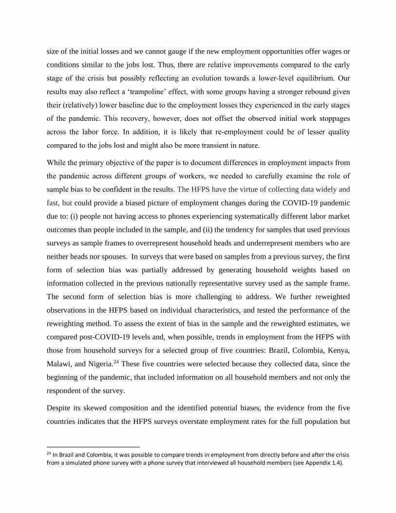
size of the initial losses and we cannot gauge if the new employment opportunities offer wages or
conditions similar to the jobs lost. Thus, there are relative improvements compared to the early
stage of the crisis but possibly reflecting an evolution towards a lower-level equilibrium. Our
results may also reflect a ‘trampoline’ effect, with some groups having a stronger rebound given
their (relatively) lower baseline due to the employment losses they experienced in the early stages
of the pandemic. This recovery, however, does not offset the observed initial work stoppages
across the labor force. In addition, it is likely that re-employment could be of lesser quality
compared to the jobs lost and might also be more transient in nature.
While the primary objective of the paper is to document differences in employment impacts from
the pandemic across different groups of workers, we needed to carefully examine the role of
sample bias to be confident in the results. The HFPS have the virtue of collecting data widely and
fast, but could provide a biased picture of employment changes during the COVID-19 pandemic
due to: (i) people not having access to phones experiencing systematically different labor market
outcomes than people included in the sample, and (ii) the tendency for samples that used previous
surveys as sample frames to overrepresent household heads and underrepresent members who are
neither heads nor spouses. In surveys that were based on samples from a previous survey, the first
form of selection bias was partially addressed by generating household weights based on
information collected in the previous nationally representative survey used as the sample frame.
The second form of selection bias is more challenging to address. We further reweighted
observations in the HFPS based on individual characteristics, and tested the performance of the
reweighting method. To assess the extent of bias in the sample and the reweighted estimates, we
compared post-COVID-19 levels and, when possible, trends in employment from the HFPS with
those from household surveys for a selected group of five countries: Brazil, Colombia, Kenya,
Malawi, and Nigeria.24 These five countries were selected because they collected data, since the
beginning of the pandemic, that included information on all household members and not only the
respondent of the survey.
Despite its skewed composition and the identified potential biases, the evidence from the five
countries indicates that the HFPS surveys overstate employment rates for the full population but
24 In Brazil and Colombia, it was possible to compare trends in employment from directly before and after the crisis from a simulated phone survey with a phone survey that interviewed all household members (see Appendix 1.4).

do reasonably well at tracking overall disparities in employment rates across gender, education,
and urban/rural groups. Furthermore, evidence from two of these countries suggests that, in
general, the HFPS accurately tracked the pattern of changes between these groups.25 In other
words, gender, education, and urban/rural gaps in employment were generally similar for heads,
who were overrepresented in the HFPS, and members that were not heads or spouses who were
underrepresented. The non-representative nature of the surveys (i.e., oversampling household
heads) leads to an upward bias in estimated employment levels, but there is little evidence that
differences between groups in employment outcomes and trends are affected by this bias.
Therefore, the “distributional” differences across groups estimated in this paper are likely to be
robust and provide meaningful insights to policy makers. The HFPS, when used with appropriate
caution, are proving to be a most valuable tool for the timely monitoring of group differences in
the impact of this massive economic shock across gender, education, and urban/rural dimensions.
25 Results are presented and discussed in Appendix 3.

References
Adams-Prassl, A., Boneva, T., Rauh, C., and Golin, M. (2020). “Inequality in the Impact of the
Coronavirus Shock: Evidence from Real Time Surveys.” Journal of Public Economics, Volume
189, September 2020, 104245.
Albanesi, J., and Kim, J. (2021) “The Gendered Impact of the COVID-19 Recession on the US
Labor Market”. Working Paper 28505. National Bureau of Economic Research, Cambridge, MA.
Alon, T. M., Doepke, M., Olmstead-Rumsey, J., and Tertilt, M. (2020). “This Time It’s Different:
The Role of Women’s Employment in a Pandemic Recession.” Working Paper 27660. National
Bureau of Economic Research, Cambridge, MA.
Alon, T., Coskun, S., Doepke, M., Koll, D., and Tertilt, M. (2021). “From Mancession to
Shecession: Women’s Employment in Regular and Pandemic Recessions.” Working Paper 28632.
National Bureau of Economic Research, Cambridge, MA.
Ambel, A. A., Mcgee, K. R., and Tsegay, A. H. (2021). “Reducing Bias in Phone Survey Samples:
Effectiveness of Reweighting Techniques Using Face-to-Face Surveys as Frames in Four African
Countries.” Policy Research Working Paper 9676,. World Bank, Washington, DC.
Andrew, A., Cattan, S., Costa Dias, M., Farquharson, Ch., Kraftman, L., Krutykova, S., Phimister,
A. y Sevilla, A. (2020). “How are Mothers and Fathers Balancing Work and Family under
Lockdown?”. IFS Briefing Note BN290, Institute for Fiscal Studies, London.
Blinder, A. S. (1973). “Wage Discrimination: Reduced Form and Structural Estimates.” Journal
of Human Resources 8: 436-55.
Boll, C., Rossen, A. and Wolf, A. (2017). “The EU Gender Earnings Gap: Job Segregation and
Working Time as Driving Factors.” Journal of Economics and Statistics 237(5): 407-52.
Brubaker, J., Kilic, T., and Wollburg, P. (2021). “Representativeness of Individual-Level Data in
COVID-19 Phone Surveys. Findings from Sub-Saharan Africa.” Policy Research Working Paper
9660, World Bank, Washington, DC.
Dang, H. A. and Nguyen, C. V. (2021). “Gender Inequality During the COVID-19 Pandemic:
Income, Expenditure, Savings and Job Loss.” World Development 140: 105296.
Del Boca, D., Oggero, N., Profeta, P., and Rossi, M. (2020). "Women’s and Men’s Work,
Housework and Childcare, Before and During COVID-19.” Review of Economics of the
Household, 18: 1001-17.
Dingel, J. I., and Neiman, B. (2020). “How Many Jobs Can Be Done at Home?” Journal of Public
Economics 189: 104235.
Fairlie, R. W., Couch, K, and Xu, H. (2020). “The Impacts of COVID-19 on Minority
Unemployment: First Evidence from April 2020 CPS Microdata.” Working Paper 27246. National
Bureau of Economic Research, Cambridge, MA.
Farre, L., Fawaz, Y., Gonzalez, L., and Graves, J. (2020). “How the COVID-19 Lockdown
Affected Gender Inequality in Paid and Unpaid Work in Spain”. IZA Discussion Paper 13434,
July 2020, Institute of Labor Economics, Bonn.

Garrote Sanchez, D., Gomez Parra, N. Ozden, C. Rijkers, B., Viollaz, M. and Winkler, H..
(forthcoming). “Who on Earth Can Work from Home?” World Bank Research Observer 36(1):
67-100.
Hatayama, M., Viollaz, M., and Winkler, H. (2020). “Jobs’ Amenability to Working from Home:
Evidence from Skills Surveys for 53 countries.” Covid Economics 211.
Horvitz, D. G., & Thompson, D. J. (1952). A generalization of sampling without replacement from
a finite universe. Journal of the American statistical Association, 47(260), 663-685.
Hupkau, C., and B. Petrongolo (2020). “Work, Care and Gender during the COVID-19 Crisis”.
IZA Working Paper 13762, Institute of Labor Economics, Bonn
ILO (International Labour Organization). (2020). “ILO Monitor: COVID-19 and the World of
Work. Fifth Edition: Updated Estimates and Analysis.”
https://www.ilo.org/wcmsp5/groups/public/---dgreports/---
dcomm/documents/briefingnote/wcms_749399.pdf
Kalton, G., & Flores-Cervantes, I. (2003). Weighting methods. Journal of official statistics, 19(2),
81.
Khamis, M., Prinz, D. Newhouse, D., Palacios-Lopez, A., Pape, U. and Weber, M. (2021). “The
Early Labor Market Impacts of COVID-19 in Developing Countries: Evidence from High-Frequency
Phone Surveys.” Policy Research Working Paper No. 9510, World Bank, Washington, DC.
Kikuchi, S., Kitao, S. Mikoshiba, M. (2021). “Who Suffers from the COVID-19 Shocks? Labor
Market Heterogeneity and Welfare Consequences in Japan.” Journal of the Japanese and
International Economies 59: 101117.
Kurth, T., Walker, A. M., Glynn, R. J., Chan, K. A., Gaziano, J. M., Berger, K., & Robins, J. M.
(2006). Results of multivariable logistic regression, propensity matching, propensity adjustment,
and propensity-based weighting under conditions of nonuniform effect. American journal of
epidemiology, 163(3), 262-270.
Lee, S. Y., Park, M. and Shin, Y. (2021). “Hit Harder, Recover Slower? Unequal Employment
Effects of the COVID-19 Shock.” NBER Working Paper No. 28354. National Bureau of Economic
Research, Cambridge, MA.
Lundberg, S. (1985). “The Added Worker Effect.” Journal of Labor Economics 3(1, Part 1): 11-
37.
Lyttelton, T., Zang, E., and Musick, K. (2020). Gender Differences in Telecommuting and
Implications for Inequality at Home and Work. Available at SSRN 3645561.
Mongey, S., Pilossoph, L., and Weinberg, A. (2020). “Which Workers Bear the Burden of Social
Distancing Policies?” Working Paper 27085. National Bureau of Economic Research, Cambridge,
MA.
Montenovo, L., Jiang, X., Rojas, F. L., Schmutte, I. M., Simon, K. I., Weinberg, B. A., and Wing,
C. (2020). “Determinants of Disparities in COVI-19 Job Losses.” Working Paper 27132. National
Bureau of Economic Research, Cambridge, MA
Oaxaca, R. (1973). “Male-Female Wage Differentials in Urban Labor markets.” International
Economic Review 14: 693-709.

Qian, Y., and Fuller, S. (forthcoming). “COVID-19 and the Gender Employment Gap among
Parents of Young Children.” Gender and Society.
Queisser, M., Adema, W., and Clarke, C. (2020). “COVID-19, Employment and Women in OECD
Countries”, VoxEU.org, 22 April.
Robins, J. M., Rotnitzky, A., & Zhao, L. P. (1995). Analysis of semiparametric regression models
for repeated outcomes in the presence of missing data. Journal of the american statistical
association, 90(429), 106-121.
Sevilla, A., and Smith, S. (2020). “Baby Steps: The Gender Division of Childcare During the
COVID-19 pandemic.” Covid Economics 23.
Schneeweiss, S., Rassen, J. A., Glynn, R. J., Avorn, J., Mogun, H., & Brookhart, M. A. (2009).
High-dimensional propensity score adjustment in studies of treatment effects using health care
claims data. Epidemiology, 20(4), 512.
Skoufias, E. and Parker, S. (2006). “Job Loss and Family Adjustments in Work and Schooling
during the Mexican Peso Crisis.” Journal of Population Economics 19(1): 163–81.
Taş, E., Reimão M. E. and Orlando, M. E. (2014). “Gender, Ethnicity, and Cumulative
Disadvantage in Education Outcomes.” World Development 64: 538-53.
Wooldridge, J. M. (2002). Inverse probability weighted M-estimators for sample selection,
attrition, and stratification. Portuguese Economic Journal, 1(2), 117-139.
World Bank (2021a). “The Gendered Impacts of COVID-19 on Labor Markets in Latin America
and the Caribbean”. Gender Innovation LAB for Latin America and the Caribbean Policy Brief,
World Bank, Washington, DC.
World Bank (2021b). “The Socioeconomic of COVID-19 in EAP”. Background Paper for the
study From Containment to Recovery, World Bank East Asia and Pacific Economic Update,
October 2020, World Bank, Washington, DC.

Appendix 1: Figures and tables
1. Sample size and data description
Table A1. Summary statistics for survey waves conducted between January and August 2020
(unweighted)
Source: HFPS.
Region
code
Country code Country Survey month in
2020
Full sample
size (Jan.-
Aug. waves)
Young
(under
age 25)
Male Low
education
level
Urban
location
Stopped
working
Employed Changed
job
Self-
employed
Employee
EAP KHM Cambodia 5, 8 1.302 0.04 0.52 n.a 0.32 0.14 0.71 0.07 0.22 0.28
EAP IDN Indonesia 5 8.449 0.02 0.65 0.28 0.62 0.22 0.78 0.11 0.27 0.49
EAP LAO Lao PDR 7 2.500 0.18 0.6 0.24 0.36 0.13 0.69 0.07 0.21 0.49
EAP MNG Mongolia 5, 9, 12 1.327 0.02 0.35 0.08 0.52 0.18 0.55 n.a 0.25 0.52
EAP MMR Myanmar 5, 6, 8, 10 4.500 0.11 0.57 0.35 0.31 0.58 0.48 0.05 n.a n.a
EAP PNG Papua New Guinea 6 3.115 0.25 0.7 0.38 0.5 0.18 0.82 0.04 n.a n.a
EAP PHL Philippines 8 9.448 0.14 0.36 0.08 0.8 0.26 0.56 0.18 n.a n.a
EAP SLB Solomon Islands 6 2.665 0.26 0.61 0.21 0.68 0.2 0.52 0.13 n.a n.a
EAP VNM Vietnam 6 6.210 0.02 0.54 n.a 0.29 0.03 0.69 0.06 0.2 0.37
ECA BGR Bulgaria 7 1.510 0.08 0.48 0.01 0.74 0.19 0.81 n.a n.a n.a
ECA HRV Croatia 6 1.500 0.03 0.35 0.11 0.63 0.27 0.73 n.a n.a n.a
ECA POL Poland 0 1.537 0.1 0.49 0.06 0.62 0.22 0.78 n.a 0.2 0.67
ECA ROU Romania 5 1.512 0.05 0.35 0.03 0.58 0.25 0.75 n.a n.a n.a
ECA UZB Uzbekistan 4, 5, 6, 7, 8 7.643 0.04 0.45 n.a 0.23 0.5 0.31 n.a 0.2 0.55
LAC BOL Bolivia 5, 6, 7 2.456 0.18 0.51 0.13 0.75 0.69 0.41 0.18 0.48 0.47
LAC CHL Chile 5, 7, 8 2.306 0.06 0.46 0.12 0.8 0.32 0.49 0.06 0.2 0.76
LAC COL Colombia 6, 7, 8 2.368 0.1 0.39 0.25 0.74 0.51 0.4 0.08 0.34 0.6
LAC CRI Costa Rica 5, 7, 8 2.095 0.14 0.48 0.52 0.51 0.35 0.55 0.07 0.33 0.61
LAC DOM Dominican Rep. 5, 7, 8 2.147 0.15 0.47 0.34 0.82 0.51 0.45 0.08 0.32 0.63
LAC ECU Ecuador 5, 6, 7 3.105 0.11 0.5 0.2 0.77 0.52 0.46 0.18 0.45 0.53
LAC SLV El Salvador 6, 7, 8 2.033 0.14 0.52 0.29 n.a 0.54 0.5 0.14 0.32 0.6
LAC GTM Guatemala 5, 7, 8 2.067 0.22 0.51 0.18 n.a 0.39 0.59 0.12 0.39 0.55
LAC HND Honduras 6, 7, 8 1.878 0.17 0.45 0.35 n.a 0.53 0.41 0.1 0.38 0.56
LAC PRY Paraguay 6, 7, 8 1.658 0.15 0.48 0.22 0.78 0.43 0.59 0.09 0.41 0.54
LAC PER Peru 5, 6, 7 2.662 0.16 0.48 0.1 0.77 0.59 0.46 0.19 0.42 0.5
LAC LCA St. Lucia 5 1.093 0.02 0.45 n.a 0.57 0.46 0.36 0.05 0.31 0.61
MNA DJI Djibouti 0 2.943 0.1 0.53 n.a 0.67 0.26 0.69 n.a 0.29 0.33
SSA BFA Burkina Faso 6, 7, 9 4.171 0.02 0.81 n.a 0.68 0.11 0.8 0.07 0.56 0.2
SSA CAF Central African Rep. 0, 6 1.865 0.19 0.64 0.41 n.a 0.37 0.7 n.a n.a n.a
SSA ETH Ethiopia 4, 5, 6, 8, 9, 10 12.177 0.12 0.63 n.a 0.7 0.17 0.74 0.01 0.49 0.42
SSA GHA Ghana 6 3.250 0.03 0.68 0.3 0.6 0.28 0.72 n.a n.a n.a
SSA KEN Kenya 6 5.389 0.14 0.51 0.5 0.49 0.08 0.5 n.a n.a n.a
SSA MDG Madagascar 6 1.228 0.06 0.65 0.36 0.72 0.1 0.6 n.a 0.52 0
SSA MWI Malawi 6, 7, 8, 9 4.979 0.11 0.61 0.54 0.37 0.13 0.85 0.04 0.35 0.34
SSA MLI Mali 0, 6, 7 9.268 0.01 0.89 n.a 0.67 0.29 0.63 n.a 0.65 0.23
SSA NGA Nigeria 4, 6, 7, 8 7.316 0.05 0.73 n.a 0.39 0.5 0.69 0.05 0.35 0.15
SSA SSD South Sudan 5 1.213 0.3 0.66 0.46 0.75 0.39 0.41 0.21 0.37 0.35
SSA UGA Uganda 6 2.196 0.05 0.52 0.65 0.26 0.17 0.69 0.15 n.a n.a
SSA ZMB Zambia 0 1.576 0.31 0.56 0.06 0.64 0.26 0.55 0.17 n.a n.a
SSA ZWE Zimbabwe 6, 7 3.340 0.05 0.49 n.a 0.26 0.2 0.48 0.05 0.22 0.33
All regions All countries All countries Full sample 139.997 0.1 0.56 0.26 0.56 0.26 0.6 0.08 0.36 0.41
All regions All countries All countries Std. deviation - 0.3 0.5 0.44 0.5 0.44 0.49 0.28 0.48 0.49
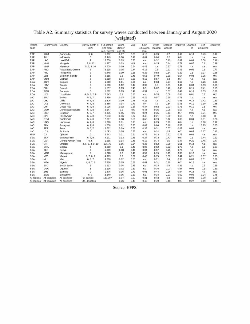
Table A2. Summary statistics for survey waves conducted between January and August 2020
(weighted)
Source: HFPS.
Region
code
Country code Country Survey month in
2020
Full sample
size (Jan.-
Aug. waves)
Young
(Under
age 25)
Male Low
education
level
Urban
location
Stopped
working
Employed Changed
job
Self-
employed
Employee
EAP KHM Cambodia 5, 8 1.302 0.17 0.53 0.16 0.73 0.7 0.42 0.18 0.49 0.47
EAP IDN Indonesia 5 8.449 0.08 0.47 0.01 0.64 0.2 0.8 n.a n.a n.a
EAP LAO Lao PDR 7 2.500 0.03 0.83 n.a 0.32 0.12 0.82 0.08 0.58 0.11
EAP MNG Mongolia 5, 9, 12 1.327 0.03 0.5 n.a 0.15 0.14 0.71 0.07 0.2 0.29
EAP MMR Myanmar 5, 6, 8, 10 4.500 0.19 0.64 0.43 n.a 0.33 0.71 n.a n.a n.a
EAP PNG Papua New Guinea 6 3.115 0.05 0.44 0.13 0.8 0.33 0.46 0.06 0.2 0.77
EAP PHL Philippines 8 9.448 0.09 0.38 0.28 0.68 0.54 0.39 0.1 0.37 0.56
EAP SLB Solomon Islands 6 2.665 0.1 0.45 0.56 0.49 0.39 0.54 0.08 0.35 0.6
EAP VNM Vietnam 6 6.210 0.04 0.51 0.18 0.57 0.3 0.7 n.a n.a n.a
ECA BGR Bulgaria 7 1.510 0.11 0.55 n.a 0.63 0.27 0.69 n.a 0.26 0.36
ECA HRV Croatia 6 1.500 0.12 0.47 0.39 0.8 0.51 0.44 0.08 0.33 0.63
ECA POL Poland 0 1.537 0.13 0.43 0.3 0.62 0.48 0.43 0.15 0.41 0.55
ECA ROU Romania 5 1.512 0.13 0.49 0.34 n.a 0.57 0.49 0.16 0.33 0.59
ECA UZB Uzbekistan 4, 5, 6, 7, 8 7.643 0.1 0.73 n.a 0.33 0.08 0.85 0.01 0.7 0.2
LAC BOL Bolivia 5, 6, 7 2.456 0.03 0.69 0.29 0.57 0.29 0.71 n.a n.a n.a
LAC CHL Chile 5, 7, 8 2.306 0.19 0.48 0.22 n.a 0.42 0.56 0.13 0.42 0.53
LAC COL Colombia 6, 7, 8 2.368 0.14 0.43 0.4 n.a 0.54 0.41 0.11 0.39 0.55
LAC CRI Costa Rica 5, 7, 8 2.095 0.02 0.66 0.37 0.62 0.23 0.76 0.11 0.3 0.5
LAC DOM Dominican Republic 5, 7, 8 2.147 0.2 0.5 0.44 0.36 0.08 0.57 n.a n.a n.a
LAC ECU Ecuador 5, 6, 7 3.105 0.15 0.6 0.24 0.35 0.13 0.7 0.06 0.21 0.5
LAC SLV El Salvador 6, 7, 8 2.033 0.06 0.72 0.48 0.21 0.08 0.66 n.a 0.48 0
LAC GTM Guatemala 5, 7, 8 2.067 0.08 0.59 0.68 0.19 0.12 0.85 0.04 0.31 0.28
LAC HND Honduras 6, 7, 8 1.878 0.01 0.91 n.a 0.29 0.29 0.6 n.a 0.68 0.17
LAC PRY Paraguay 6, 7, 8 1.658 0.02 0.35 0.07 0.66 0.19 0.53 n.a 0.25 0.55
LAC PER Peru 5, 6, 7 2.662 0.09 0.57 0.38 0.31 0.57 0.48 0.04 n.a n.a
LAC LCA St. Lucia 5 1.093 0.05 0.75 n.a 0.32 0.5 0.7 0.05 0.37 0.12
MNA DJI Djibouti 0 2.943 0.21 0.51 0.73 0.13 0.22 0.78 0.04 n.a n.a
SSA BFA Burkina Faso 6, 7, 9 4.171 0.13 0.48 0.24 0.73 0.43 0.6 0.1 0.44 0.52
SSA CAF Central African Republic 0, 6 1.865 0.14 0.48 0.13 0.74 0.6 0.47 0.21 0.46 0.47
SSA ETH Ethiopia 4, 5, 6, 8, 9, 10 12.177 0.16 0.34 0.36 0.52 0.28 0.51 0.18 n.a n.a
SSA GHA Ghana 6 3.250 0.1 0.49 0.06 0.62 0.22 0.78 n.a 0.2 0.67
SSA KEN Kenya 6 5.389 0.08 0.48 0.04 0.57 0.25 0.75 n.a n.a n.a
SSA MDG Madagascar 6 1.228 0.2 0.48 0.59 0.15 0.15 0.38 0.12 n.a n.a
SSA MWI Malawi 6, 7, 8, 9 4.979 0.3 0.66 0.46 0.75 0.39 0.41 0.21 0.37 0.35
SSA MLI Mali 0, 6, 7 9.268 0.02 0.53 n.a 0.71 0.4 0.38 0.05 0.31 0.59
SSA NGA Nigeria 4, 6, 7, 8 7.316 0.05 0.52 0.61 0.31 0.19 0.7 0.12 n.a n.a
SSA SSD South Sudan 5 1.213 0.04 0.45 n.a 0.23 0.5 0.32 n.a 0.2 0.55
SSA UGA Uganda 6 2.196 0.02 0.53 n.a 0.35 0.03 0.67 0.06 0.2 0.39
SSA ZMB Zambia 0 1.576 0.35 0.49 0.05 0.44 0.26 0.54 0.18 n.a n.a
SSA ZWE Zimbabwe 6, 7 3.340 0.05 0.51 n.a 0.34 0.21 0.52 0.06 0.24 0.45
All regions All countries All countries Full sample 139.997 0.07 0.57 0.31 0.43 0.3 0.57 0.08 0.39 0.36
All regions All countries All countries Std. deviation - 0.26 0.49 0.46 0.49 0.46 0.5 0.27 0.49 0.48

Table A3. Summary statistics for survey waves conducted in April or May 2020 (unweighted)
Source: HFPS.
Table A4. Summary statistics for survey waves conducted in April or May 2020 (weighted)
Source: HFPS.
Region
code
Country
code
Country Full sample
size (April &
May waves)
Young
(under
age 25)
Male Low
education
level
Urban
location
Stopped
working
Employed Changed
job
Self-
employed
Employee
LAC BOL Bolivia 1.075 0.18 0.5 0.13 0.75 0.69 0.27 0.14 0.47 0.49
EAP KHM Cambodia 694 0.04 0.52 n.a 0.32 0.14 0.72 0.07 0.26 0.27
LAC CHL Chile 1.000 0.07 0.45 0.13 0.8 0.32 0.52 0.04 0.2 0.78
LAC CRI Costa Rica 801 0.15 0.49 0.52 0.51 0.35 0.52 0.04 0.3 0.64
LAC DOM Dominican Rep. 807 0.15 0.47 0.34 0.82 0.51 0.37 0.04 0.29 0.66
LAC ECU Ecuador 1.227 0.11 0.51 0.21 0.76 0.52 0.38 0.15 0.43 0.54
SSA ETH Ethiopia 6.249 0.12 0.63 n.a 0.7 0.17 0.71 0.01 0.49 0.43
LAC GTM Guatemala 806 0.23 0.5 0.18 n.a 0.39 0.51 0.08 0.39 0.56
EAP IDN Indonesia 8.449 0.02 0.65 0.28 0.62 0.22 0.78 0.11 0.27 0.49
EAP MNG Mongolia 1.327 0.02 0.35 0.08 0.52 0.18 0.55 n.a 0.25 0.52
EAP MMR Myanmar 1.500 0.1 0.58 0.44 0.31 0.58 0.34 0.06 n.a n.a
SSA NGA Nigeria 1.942 0.05 0.73 n.a 0.39 0.5 0.43 n.a 0.3 0.19
LAC PER Peru 1.000 0.16 0.48 0.1 0.77 0.59 0.34 0.13 0.38 0.55
ECA ROU Romania 1.512 0.05 0.35 0.03 0.58 0.25 0.75 n.a n.a n.a
SSA SSD South Sudan 1.213 0.3 0.66 0.46 0.75 0.39 0.41 0.21 0.37 0.35
LAC LCA St. Lucia 1.093 0.02 0.45 n.a 0.57 0.46 0.36 0.05 0.31 0.61
ECA UZB Uzbekistan 3.058 0.04 0.45 n.a 0.23 0.5 0.25 n.a 0.13 0.64
All regions All countries All countries 33.753 0.08 0.56 0.24 0.58 0.36 0.53 0.07 0.35 0.48
All regions All countries Std. deviation - 0.27 0.5 0.43 0.49 0.48 0.5 0.26 0.48 0.5
Region
code
Country
code
Country Full sample
size (April &
May waves)
Young
(Under
age 25)
Male Low
education
level
Urban
location
Stopped
working
Employed Changed
job
Self-
employed
Employee
LAC BOL Bolivia 1.075 0.17 0.52 0.16 0.73 0.7 0.26 0.16 0.49 0.46
EAP KHM Cambodia 694 0.04 0.51 n.a 0.15 0.14 0.71 0.08 0.23 0.29
LAC CHL Chile 1.000 0.06 0.43 0.13 0.8 0.33 0.49 0.04 0.19 0.78
LAC CRI Costa Rica 801 0.11 0.46 0.55 0.49 0.39 0.49 0.04 0.32 0.64
LAC DOM Dominican Republic 807 0.12 0.47 0.39 0.8 0.51 0.37 0.06 0.3 0.66
LAC ECU Ecuador 1.227 0.13 0.45 0.3 0.61 0.48 0.37 0.12 0.39 0.56
SSA ETH Ethiopia 6.249 0.1 0.73 n.a 0.33 0.08 0.83 0.01 0.7 0.2
LAC GTM Guatemala 806 0.18 0.47 0.22 n.a 0.42 0.47 0.09 0.4 0.55
EAP IDN Indonesia 8.449 0.02 0.66 0.37 0.62 0.23 0.76 0.11 0.3 0.5
EAP MNG Mongolia 1.327 0.02 0.35 0.07 0.66 0.19 0.53 n.a 0.25 0.55
EAP MMR Myanmar 1.500 0.08 0.58 0.45 0.31 0.57 0.35 0.05 n.a n.a
SSA NGA Nigeria 1.942 0.05 0.75 n.a 0.31 0.5 0.43 n.a 0.32 0.17
LAC PER Peru 1.000 0.13 0.47 0.13 0.72 0.6 0.33 0.15 0.43 0.52
ECA ROU Romania 1.512 0.08 0.48 0.04 0.57 0.25 0.75 n.a n.a n.a
SSA SSD South Sudan 1.213 0.3 0.66 0.46 0.75 0.39 0.41 0.21 0.37 0.35
LAC LCA St. Lucia 1.093 0.02 0.53 n.a 0.71 0.4 0.38 0.05 0.31 0.59
ECA UZB Uzbekistan 3.058 0.04 0.45 n.a 0.23 0.5 0.26 n.a 0.13 0.64
All regions All countries All countries 33.753 0.05 0.61 0.33 0.47 0.33 0.54 0.08 0.38 0.43
All regions All countries Std. deviation - 0.21 0.49 0.47 0.5 0.47 0.5 0.27 0.48 0.49

Table A5. Summary statistics for survey waves conducted in August 2020 (unweighted)
Source: HFPS.
Table A6. Summary statistics for survey waves conducted in August 2020 (weighted)
Source: HFPS.
2. Rate of work stoppage by groups
Section 3.1 showed that, for the average of the 40 countries under analysis, women, youth, less
educated, and urban workers were affected the most by job loss in the first months of the pandemic
(between April and June). Figures A1 to A4 present the between-group differences in the rate of
work stoppage differentiating by country.
Region
code
Country
code
Country Full sample
size (August
waves)
Young
(under
age 25)
Male Low
education
level
Urban
location
Stopped
working
Employed Changed
job
Self-
employed
Employee
EAP KHM Cambodia 608 0.03 0.51 n.a 0.33 n.a 0.71 0.06 0.18 0.29
LAC CHL Chile 684 0.06 0.46 0.12 0.8 n.a 0.49 n.a 0.21 0.74
LAC COL Colombia 638 0.08 0.4 0.27 0.75 n.a 0.43 n.a 0.35 0.57
LAC CRI Costa Rica 658 0.13 0.47 0.53 0.52 n.a 0.58 n.a 0.35 0.59
LAC DOM Dominican Rep. 667 0.14 0.46 0.34 0.82 n.a 0.48 n.a 0.33 0.62
LAC SLV El Salvador 604 0.14 0.52 0.29 n.a n.a 0.59 n.a 0.38 0.55
SSA ETH Ethiopia 2.874 0.12 0.62 n.a 0.71 n.a 0.78 0.01 0.48 0.42
LAC GTM Guatemala 636 0.22 0.52 0.17 n.a n.a 0.65 n.a 0.39 0.54
LAC HND Honduras 521 0.17 0.44 0.36 n.a n.a 0.49 n.a 0.36 0.58
SSA MWI Malawi 1.616 0.11 0.58 0.67 0.37 n.a 0.95 0.03 0.35 0.33
EAP MMR Myanmar 1.500 0.11 0.53 0.23 0.31 n.a 0.81 0.02 n.a n.a
SSA NGA Nigeria 1.781 0.05 0.73 n.a 0.39 n.a 0.84 0.03 0.36 0.14
LAC PRY Paraguay 457 0.16 0.47 0.23 0.78 n.a 0.69 n.a 0.4 0.54
EAP PHL Philippines 9.448 0.14 0.36 0.08 0.8 0.26 0.56 0.18 n.a n.a
ECA UZB Uzbekistan 1.530 0.05 0.45 n.a 0.23 n.a 0.36 n.a 0.25 0.52
All regions All countries All countries 24.222 0.12 0.48 0.16 0.63 0.26 0.63 0.1 0.37 0.41
All regions All countries Std. deviation - 0.32 0.5 0.36 0.48 0.44 0.48 0.3 0.48 0.49

In 88% of the countries the rate of work stoppage was larger for women than for men and in 55%,
the gender gap in favor of women, i.e., women being more likely to have lost their job, was
statistically significant (Figure A1). The largest female rate of work stoppage appears in Bolivia
where 74% of surveyed women stopped working since the start of the pandemic. On the other
hand, the largest gender gap is reported in Costa Rica, where the rate of work stoppage was 25
percentage points larger for women than for men.
When grouping by age, the country-level evidence indicates that the age gap in the rate of work
stoppage was larger for young workers in 63% of the countries, being statistically significant in
only 18% of them (Figure A2). Again, Bolivia is the country with the largest rate of work stoppage
for the disadvantage group –i.e., young workers—who reported a rate of 73%. The largest age gap
appears in Croatia where the rate of work stoppage of young workers surpassed the rate of adult
workers by 36 percentage points.
The comparison by level of education shows that in 70% of the countries the rate of work stoppage
was larger for low-educated workers and in 23% of the countries the difference was statistically
significant (Figure A3). Peru is the country where low-educated workers were hit hardest by job
loss. In this country, the rate of work stoppage for low-educated workers was 75%. The largest
education gap appears in Bulgaria with a difference in the rate of work stoppage between low- and
high-educated workers of 21 percentage points.
Finally, urban workers lost their jobs more than rural workers in 60% of the countries, with
statistically significant differences in 31% of them (Figure A4). Bolivia is the country with the
largest rate of work stoppage among urban workers (72%), while Ethiopia is the country where
the location gap is largest (17 percentage points).

Figure A1. Gender gaps in rate of work stoppage by country
Source: Authors’ calculations based on HFPS.
Notes: Dark (light) colors indicate that the difference between groups is (not) statistically significant at 5% level or
less.
Figure A2. Age gaps in rate of work stoppage by country
Source: Authors’ calculations based on HFPS.
Notes: Dark (light) colors indicate that the difference between groups is (not) statistically significant at 5% level or
less.

Figure A3. Education gaps in rate of work stoppage by country
Source: Authors’ calculations based on HFPS.
Notes: Dark (light) colors indicate that the difference between groups is (not) statistically significant at 5% level or
less.
Figure A4. Location gaps in rate of work stoppage by country
Source: Authors’ calculations based on HFPS.
Notes: Dark (light) colors indicate that the difference between groups is (not) statistically significant at 5% level or
less.
3. Understanding the gender gap in the rate of work stoppage
The between-group difference in the rate of work stoppage was larger when grouping by gender.
Specifically, 34% of women stopped working since the pandemic started while the rate for men
was 27%. Three possible reasons behind this result are the differential incidence of childcare

activities, the possibility of working remotely, and the pre-pandemic sectoral structure of
employment.
Regarding childcare activities, the HFPS asks to households with school age children who attended
primary or secondary school before the pandemic whether they have participated in any learning
or education services since school closure. Figure A5 presents the correlation between the average
of this variable at the country and group level and the average of the rate of work stoppage. For all
groups there is a positive association between the incidence of childcare activities and the rate of
work stoppage. The grouping by gender also reveals a steeper association for women than for men.
Figure A6 presents the correlation between the measure of amenability of working from home
developed by Hatayama et al. (2020) and the rate of work stoppage by groups. This work-from-
home measure uses pre-pandemic information on tasks performed at work, such as the intensity of
computer and internet use, the intensity of physical and manual work, and the intensity of face-to-
face interaction, and the availability of an internet connection at home. The figure separates
between two groups of countries depending on the data source use to generate the work from home
measure --i.e., the PIAAC survey or the STEP survey. The evidence indicates that for all groups a
higher amenability of working remotely protected workers from job loss. However, although
women are more likely than men to have a job that can be done from home, their rate of work
stoppage was larger.

Figure A5. Work stoppage and children learning activities by groups and countries
Source: Authors’ calculations based on HFPS.
Notes: Work stoppage rate by groups and countries and share of people in each group and country indicating that
school age children are performing learning activities since school closing.

Figure A6. Work stoppage rate and Work-from-Home measure by groups and countries
Source: Authors’ calculations based on HFPS.
Notes: Work from home measure from Hatayama, Viollaz and Winkler (2020). A higher value indicates a higher
amenability of working from home. Countries in the HFPS and PIAAC survey include Chile, Ecuador, Peru and
Polonia. Countries in the HFPS and the STEP survey include Bolivia, Colombia, Ghana, Kenya, Laos, Philippines,
El Salvador and Vietnam.
4. Change in employment by type and sector
Section 3.3 presented evidence indicating that, for all demographic groups and for the average of
all countries, workers who remained employed since the start of the pandemic tended to move
from wage employment to self-employment. Figures A7 and A8 present these changes by country.
The figures present, for each country and group, the difference between the share of wage or self-
employment before the start of the pandemic and the share by April-June of 2020. The pre-
pandemic information comes from retrospective questions available in the HFPS. In both cases,
the overtime change in employment type was statistically significant in very few cases (dark bars
or diamonds), and the between-group difference (indicated with an asterisk next to the name of the
country) was statistically insignificant for all groups and countries.

Figure A7. Change in the share of wage employment by country and groups
Source: Authors’ calculations based on HFPS.
Notes: Calculations use HFPS retrospective data as pre-COVID information. Dark (light) colors indicate that
overtime change is (not) statistically significant at 5% level or less within a group. * in the country name indicates
that the overtime change between groups is statistically significant at 5% level or less.

Figure A8. Change in the share of self-employment by country and groups
Source: Authors’ calculations based on HFPS.
Notes: Calculations use HFPS retrospective data as pre-COVID information. Dark (light) colors indicate that
overtime change is (not) statistically significant at 5% level or less within a group. * in the country name indicates
that the overtime change between groups is statistically significant at 5% level or less.
Regarding differences in employment sector, Section 3.3 reported small differences for all groups
and for the average of all countries when comparing the pre-pandemic sector of employment with
the actual sector of employment for workers who remained employed since the pandemic started.
Figures A9 to A12 present the overtime changes in the share of workers in the primary, industry,
services, and public administration sectors by country. These figures show that the overtime
change in employment sector was statistically significant in very few countries (dark bars or
diamonds), and the between-group difference (indicated with an asterisk next to the name of the
country) was not statistically significant in most of them.
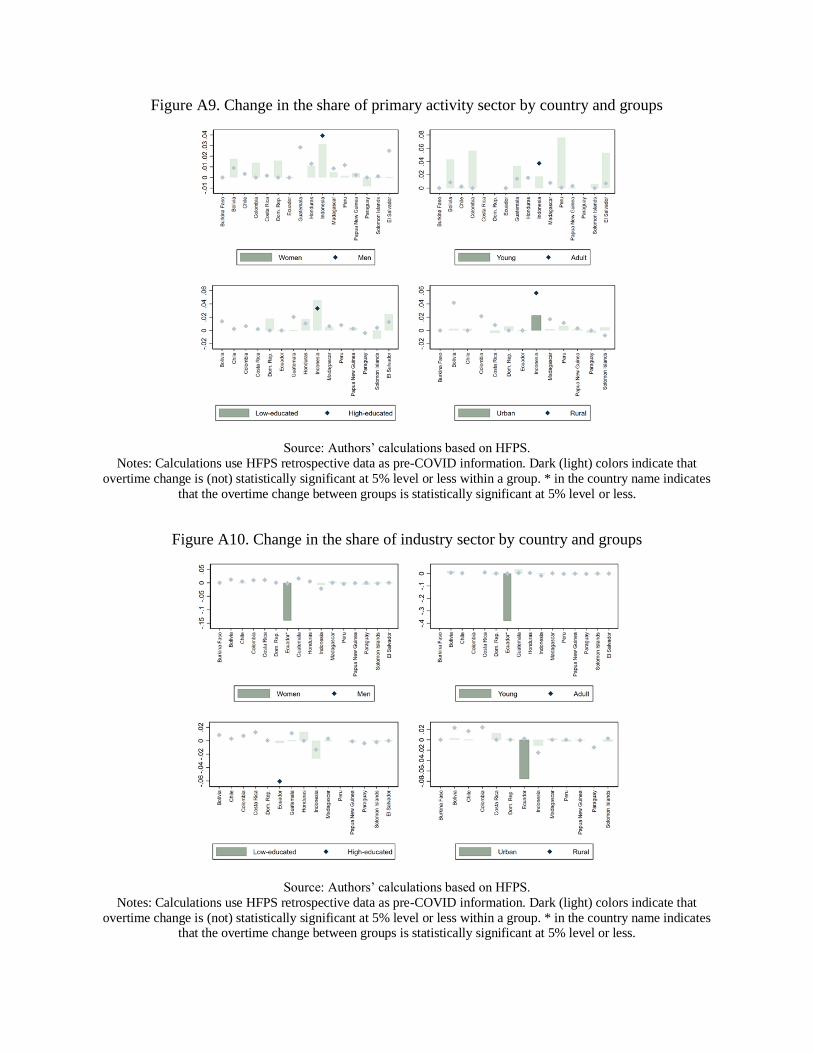
Figure A9. Change in the share of primary activity sector by country and groups
Source: Authors’ calculations based on HFPS.
Notes: Calculations use HFPS retrospective data as pre-COVID information. Dark (light) colors indicate that
overtime change is (not) statistically significant at 5% level or less within a group. * in the country name indicates
that the overtime change between groups is statistically significant at 5% level or less.
Figure A10. Change in the share of industry sector by country and groups
Source: Authors’ calculations based on HFPS.
Notes: Calculations use HFPS retrospective data as pre-COVID information. Dark (light) colors indicate that
overtime change is (not) statistically significant at 5% level or less within a group. * in the country name indicates that the overtime change between groups is statistically significant at 5% level or less.

Figure A11. Change in the share of services sector by country and groups
Source: Authors’ calculations based on HFPS.
Notes: Calculations use HFPS retrospective data as pre-COVID information. Dark (light) colors indicate that overtime change is (not) statistically significant at 5% level or less within a group. * in the country name indicates
that the overtime change between groups is statistically significant at 5% level or less.
Figure A12. Change in the share of public administration sector by country and groups
Source: Authors’ calculations based on HFPS.
Notes: Calculations use HFPS retrospective data as pre-COVID information. Dark (light) colors indicate that overtime change is (not) statistically significant at 5% level or less within a group. * in the country name indicates
that the overtime change between groups is statistically significant at 5% level or less.
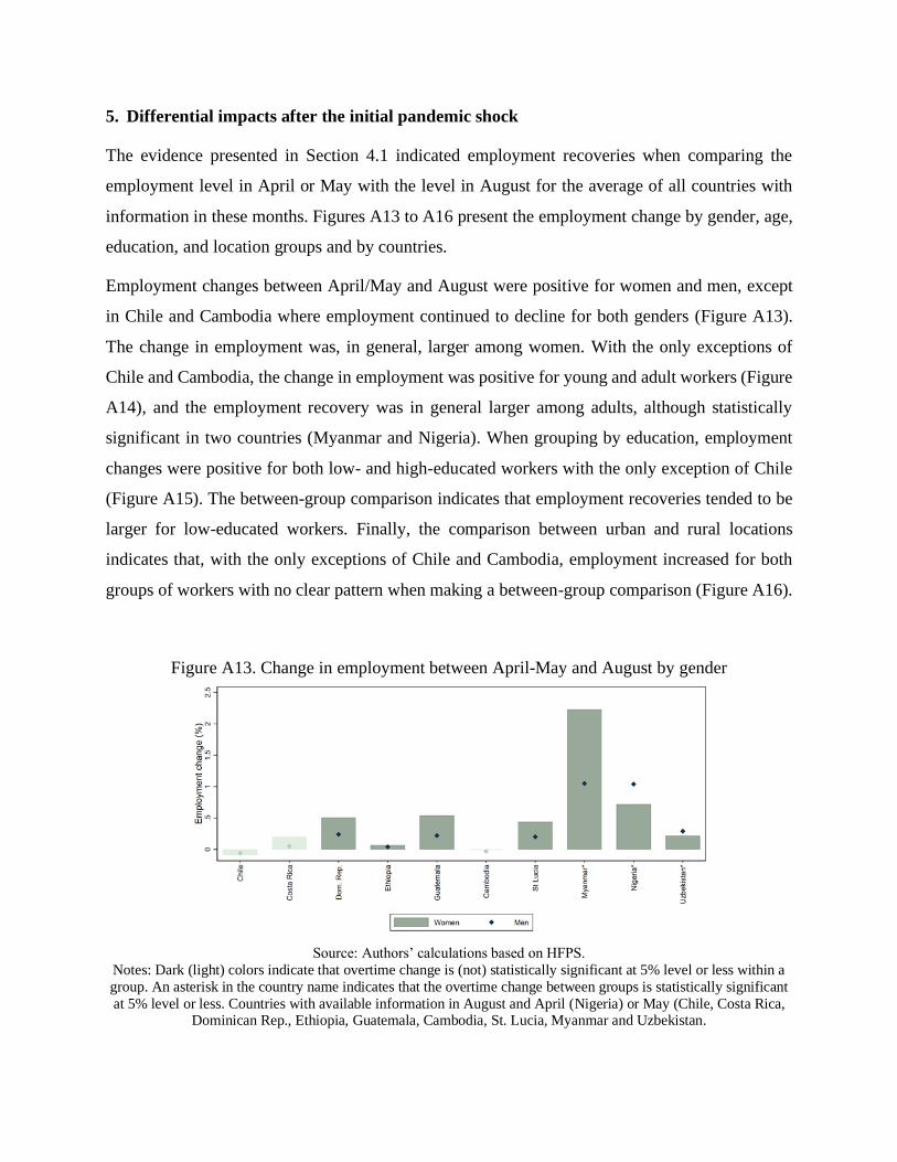
5. Differential impacts after the initial pandemic shock
The evidence presented in Section 4.1 indicated employment recoveries when comparing the
employment level in April or May with the level in August for the average of all countries with
information in these months. Figures A13 to A16 present the employment change by gender, age,
education, and location groups and by countries.
Employment changes between April/May and August were positive for women and men, except
in Chile and Cambodia where employment continued to decline for both genders (Figure A13).
The change in employment was, in general, larger among women. With the only exceptions of
Chile and Cambodia, the change in employment was positive for young and adult workers (Figure
A14), and the employment recovery was in general larger among adults, although statistically
significant in two countries (Myanmar and Nigeria). When grouping by education, employment
changes were positive for both low- and high-educated workers with the only exception of Chile
(Figure A15). The between-group comparison indicates that employment recoveries tended to be
larger for low-educated workers. Finally, the comparison between urban and rural locations
indicates that, with the only exceptions of Chile and Cambodia, employment increased for both
groups of workers with no clear pattern when making a between-group comparison (Figure A16).
Figure A13. Change in employment between April-May and August by gender
Source: Authors’ calculations based on HFPS.
Notes: Dark (light) colors indicate that overtime change is (not) statistically significant at 5% level or less within a
group. An asterisk in the country name indicates that the overtime change between groups is statistically significant
at 5% level or less. Countries with available information in August and April (Nigeria) or May (Chile, Costa Rica, Dominican Rep., Ethiopia, Guatemala, Cambodia, St. Lucia, Myanmar and Uzbekistan.

Figure A14. Change in employment between April-May and August by age
Source: Authors’ calculations based on HFPS.
Notes: Dark (light) colors indicate that overtime change is (not) statistically significant at 5% level or less within a group. An asterisk in the country name indicates that the overtime change between groups is statistically significant
at 5% level or less. Countries with available information in August and April (Nigeria) or May (Chile, Costa Rica,
Dominican Rep., Ethiopia, Guatemala, Cambodia, St. Lucia, Myanmar and Uzbekistan.
Figure A15. Change in employment between April-May and August by education
Source: Authors’ calculations based on HFPS.
Notes: Dark (light) colors indicate that overtime change is (not) statistically significant at 5% level or less within a
group. An asterisk in the country name indicates that the overtime change between groups is statistically significant
at 5% level or less. Countries with available information in August and April (Nigeria) or May (Chile, Costa Rica, Dominican Rep., Ethiopia, Guatemala, Cambodia, St. Lucia, Myanmar and Uzbekistan.

Figure A16. Change in employment between April-May and August by location
Source: Authors’ calculations based on HFPS.
Notes: Dark (light) colors indicate that overtime change is (not) statistically significant at 5% level or less within a
group. An asterisk in the country name indicates that the overtime change between groups is statistically significant
at 5% level or less. Countries with available information in August and April (Nigeria) or May (Chile, Costa Rica,
Dominican Rep., Ethiopia, Guatemala, Cambodia, St. Lucia, Myanmar and Uzbekistan.
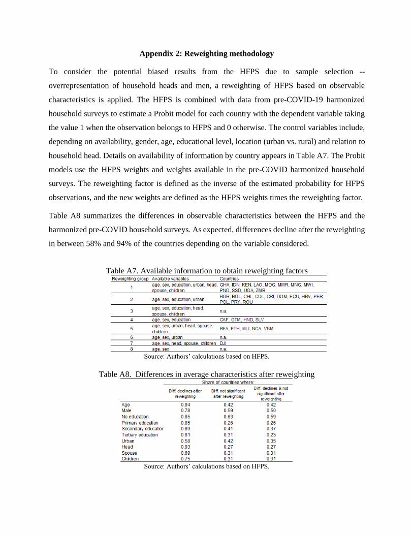
Appendix 2: Reweighting methodology
To consider the potential biased results from the HFPS due to sample selection --
overrepresentation of household heads and men, a reweighting of HFPS based on observable
characteristics is applied. The HFPS is combined with data from pre-COVID-19 harmonized
household surveys to estimate a Probit model for each country with the dependent variable taking
the value 1 when the observation belongs to HFPS and 0 otherwise. The control variables include,
depending on availability, gender, age, educational level, location (urban vs. rural) and relation to
household head. Details on availability of information by country appears in Table A7. The Probit
models use the HFPS weights and weights available in the pre-COVID harmonized household
surveys. The reweighting factor is defined as the inverse of the estimated probability for HFPS
observations, and the new weights are defined as the HFPS weights times the reweighting factor.
Table A8 summarizes the differences in observable characteristics between the HFPS and the
harmonized pre-COVID household surveys. As expected, differences decline after the reweighting
in between 58% and 94% of the countries depending on the variable considered.
Table A7. Available information to obtain reweighting factors
Source: Authors’ calculations based on HFPS.
Table A8. Differences in average characteristics after reweighting
Source: Authors’ calculations based on HFPS.

Appendix 3. Validation of HFPS sampling methodology and reweighting
Section 5.4 assesses the validity of the HFPS sampling methodology that tends to oversample
household heads or their spouses. The analysis focuses on five countries (Colombia, Brazil,
Nigeria, Kenya, and Malawi) and four reweighting methodologies. Figure A17 presents the results
obtained when using the four proposed reweighting methods: inverse propensity score, inverse
propensity score by deciles method, raking method, and raking combined with inverse propensity
score to predict between differences in employment levels. The figure confirms the results
presented in the main text. The respondents’ sample in Kenya, Nigeria and Malawi, and the
simulated phone survey in Brazil and Colombia provide good estimates –i.e., close to those
observed in the sample of all working age household members-- of between-groups differences in
employment levels when the grouping variable is balanced between samples. In general, the
reweighting methods do not improve results.
Figure A17. Between-group differences in employment levels during-COVID. In percentages
Colombia

Brazil
Nigeria
Kenya

Malawi
Source: Authors’ calculations based on GEIH (Colombia), PNAD-C (Brazil), NLPS-Wave 5 (Nigeria), World Bank
Covid-19 Rapid Response Phone Survey (Kenya), and HFPS-Wave 5 (Malawi). Notes: Dark (light) colors indicate that the difference in employment levels between groups is (not) statistically
significant at 5% level or less in the corresponding sample.
In terms of validation of employment changes using surveys with labor market information for all
household members, Table A9 shows the trends in employment changes by group in Brazil and
Colombia, the two countries for which we have data on all household members before and after
the beginning of the pandemic. By and large the differences in employment trends, in percentage
points, are comparable for each group. Moderate differences between the simulated phone survey
data and the full data are observed when comparing youth and adult works in Colombia, as the
simulated phone survey found youth employment declined 1 percentage point less than adult
employment, whereas the actual survey found that youth employment declined four percentage
points more for youth. Overall, however, the simulated phone surveys accurately reflect the greater
employment losses faced by female workers in both countries, and the greater losses faced by
younger and less educated workers in Brazil.
When using the inverse propensity score on the simulated phone survey sample, the results are
very close to the selected sample without reweighting in both countries. If anything, the
reweighting provides an estimation of changes in employment between groups that are one
percentage point off from the true value in comparison to the estimation provided by the simulated
phone survey – e.g., education groups in Colombia and Brazil.

When comparing employment changes between groups with other reweighting methods the
evidence indicates that all the methods provide results which are close to those obtained using the
simulated phone survey (Figure A18).
Table A9. Differences in Employment Changes by Groups
Source: Authors’ calculations based on GEIH (Colombia) and PNAD-C (Brazil).
Notes: The reweighting method presented in the last column is the inverse propensity score.
Pre-
COVID
During-
COVIDDifference
Pre-
COVID
During-
COVIDDifference
Pre-
COVID
During-
COVIDDifference
Panel A: Colombia
Women 0.48 0.37 -22% 0.51 0.41 -20% 0.51 0.41 -20%
Men 0.77 0.66 -15% 0.80 0.70 -12% 0.80 0.71 -12%
Difference -0.07 -0.07 -0.07
Young 0.49 0.38 -21% 0.52 0.44 -15% 0.52 0.44 -15%
Adult 0.65 0.54 -17% 0.67 0.56 -15% 0.67 0.57 -15%
Difference -0.04 0.01 0.01
Low-educated 0.55 0.45 -18% 0.58 0.50 -14% 0.59 0.51 -14%
High-educated 0.65 0.54 -18% 0.68 0.58 -16% 0.69 0.58 -16%
Difference 0.00 0.01 0.02
Urban 0.62 0.50 -20% 0.65 0.54 -18% 0.65 0.54 -18%
Rural 0.62 0.54 -12% 0.65 0.59 -9% 0.65 0.59 -9%
Difference -0.08 -0.08 -0.08
All people 0.62 0.51 -18% 0.65 0.55 -15% 0.65 0.55 -15%
Panel B: Brazil
Women 0.47 0.40 -16% 0.47 0.40 -15% 0.49 0.42 -15%
Men 0.66 0.58 -13% 0.69 0.62 -10% 0.70 0.63 -10%
Difference -0.03 -0.04 -0.04
Young 0.39 0.29 -25% 0.48 0.37 -23% 0.47 0.37 -22%
Adult 0.61 0.53 -13% 0.58 0.51 -12% 0.61 0.54 -11%
Difference -0.12 -0.11 -0.11
Low-educated 0.53 0.44 -16% 0.53 0.46 -14% 0.55 0.48 -14%
High-educated 0.79 0.74 -6% 0.78 0.73 -6% 0.80 0.75 -6%
Difference -0.10 -0.08 -0.07
Urban 0.57 0.49 -14% 0.58 0.51 -12% 0.60 0.52 -12%
Rural 0.48 0.42 -14% 0.50 0.44 -12% 0.52 0.46 -11%
Difference 0.00 0.00 -0.01
All people 0.56 0.48 -14% 0.57 0.50 -12% 0.59 0.52 -12%
Full survey Simulated Phone Survey Simulated PS - Reweighted

Figure A18. Differences in Employment Changes by Groups. In percentage points
Colombia
Brazil
Source: Authors’ calculations based on GEIH (Colombia) and PNAD-C (Brazil).
Notes: Dark (light) colors indicate that the difference in employment change between groups is (not) statistically
significant at 5% level or less in the corresponding sample.

Most Recent Jobs Working Papers:
59. Determinantes Del Crecimiento De La Demanda Laboral Y De La Productividad Del Sector Privado (Spanish) (2021) Mariana Vijil
58. The Early Labor Market Impacts of Covid-19 In Developing Countries: Evidence from High-Frequency Phone Surveys (2021) Melanie Khamis, Daniel Prinz, David Newhouse, Amparo Palacios-Lopez, Utz Pape and Michael Weber
57. Empirical Evidence on Firm Growth and Jobs in Developing Countries (2020) Johanne Buba, Alvaro Gonzalez and Anam Rizvi 56. Promoting Female Labor Force Participation (2020) Svetlana Pimkina and Luciana de La Flor
55. Structural Transformation and Labor Market Performance In Ghana (2020) Mpumelelo Nxumalo and Dhushyanth Raju
54. Just Coal Transition in Western Macedonia, Greece-Insights from the Labor Market (2020) Luc Christiaensen and Céline Ferré
53. Insights from Surveys on Business and Enterprises in South Sudan: Jobs, Recovery, and Peacebuilding in Urban South Sudan – Technical Report IV (2020) Arden Finn and Jan von der Goltz
52. Job Outcomes in The Towns Of South Sudan: Jobs, Recovery, And Peacebuilding In Urban South Sudan – Technical Report III (2020) Jan von der Goltz, Mira Saidi, Augustino Ting Mayai, and Melissa Williams.
51. The Macroeconomic Environment for Jobs in South Sudan: Jobs, Recovery, and Peacebuilding in Urban South Sudan – Technical Report II (2020) Joseph Mawejje
50. Job Outcomes in the Towns of South Sudan: Jobs, Recovery, and Peacebuilding in Urban South Sudan- Technical Report I (2020) Arden Finn, Jan von der Goltz, Mira Saidi, and Ambika Sharma.
Click here for full Jobs Paper Series

Address: 1776 G St, NW, Washington, DC 20006 Website: http://www.worldbank.org/en/topic/jobsanddevelopment
Twitter: @WBG_Jobs Blog: https://blogs.worldbank.org/jobs/