Embed Size (px)
Citation preview
John Butcher’s tutorials
Implicit Runge–Kutta methods
1
2−
√
3
6
1
4
1
4−
√
3
6
1
2+
√
3
6
1
4+
√
3
6
1
4
1
2
1
2
Implicit Runge–Kutta methods
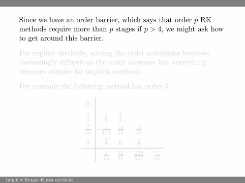
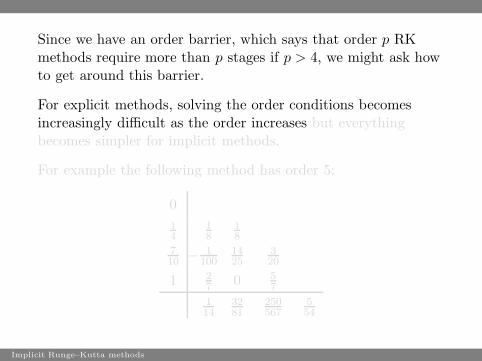
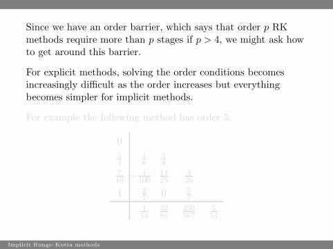
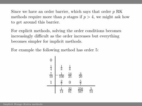
Since we have an order barrier, which says that order p RKmethods require more than p stages if p > 4, we might ask howto get around this barrier.
For explicit methods, solving the order conditions becomesincreasingly difficult as the order increases but everythingbecomes simpler for implicit methods.
For example the following method has order 5:
0
14
18
18
710 − 1
1001425
320
1 27 0 5
7
114
3281
250567
554
Implicit Runge–Kutta methods
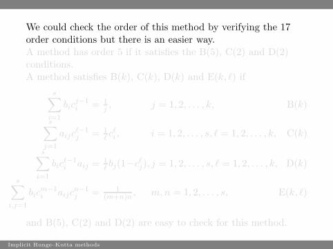
We could check the order of this method by verifying the 17order conditions but there is an easier way.A method has order 5 if it satisfies the B(5), C(2) and D(2)conditions.A method satisfies B(k), C(k), D(k) and E(k, ℓ) if
s∑
i=1
bicj−1i = 1
j, j = 1, 2, . . . , k, B(k)
s∑
j=1
aijcℓ−1j = 1
ℓcℓi , i = 1, 2, . . . , s, ℓ = 1, 2, . . . , k, C(k)
s∑
i=1
bicℓ−1i aij = 1
ℓbj(1−cℓ
j), j = 1, 2, . . . , s, ℓ = 1, 2, . . . , k, D(k)
s∑
i,j=1
bicm−1i aijc
n−1j = 1
(m+n)n , m, n = 1, 2, . . . , s, E(k, ℓ)
and B(5), C(2) and D(2) are easy to check for this method.
Implicit Runge–Kutta methods
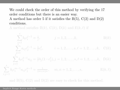
We could check the order of this method by verifying the 17order conditions but there is an easier way.A method has order 5 if it satisfies the B(5), C(2) and D(2)conditions.A method satisfies B(k), C(k), D(k) and E(k, ℓ) if
s∑
i=1
bicj−1i = 1
j, j = 1, 2, . . . , k, B(k)
s∑
j=1
aijcℓ−1j = 1
ℓcℓi , i = 1, 2, . . . , s, ℓ = 1, 2, . . . , k, C(k)
s∑
i=1
bicℓ−1i aij = 1
ℓbj(1−cℓ
j), j = 1, 2, . . . , s, ℓ = 1, 2, . . . , k, D(k)
s∑
i,j=1
bicm−1i aijc
n−1j = 1
(m+n)n , m, n = 1, 2, . . . , s, E(k, ℓ)
and B(5), C(2) and D(2) are easy to check for this method.
Implicit Runge–Kutta methods
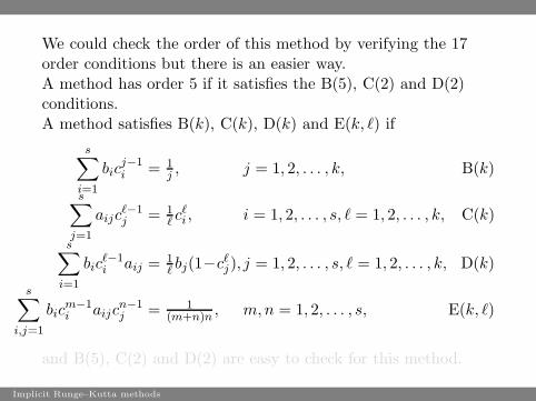
We could check the order of this method by verifying the 17order conditions but there is an easier way.A method has order 5 if it satisfies the B(5), C(2) and D(2)conditions.A method satisfies B(k), C(k), D(k) and E(k, ℓ) if
s∑
i=1
bicj−1i = 1
j, j = 1, 2, . . . , k, B(k)
s∑
j=1
aijcℓ−1j = 1
ℓcℓi , i = 1, 2, . . . , s, ℓ = 1, 2, . . . , k, C(k)
s∑
i=1
bicℓ−1i aij = 1
ℓbj(1−cℓ
j), j = 1, 2, . . . , s, ℓ = 1, 2, . . . , k, D(k)
s∑
i,j=1
bicm−1i aijc
n−1j = 1
(m+n)n , m, n = 1, 2, . . . , s, E(k, ℓ)
and B(5), C(2) and D(2) are easy to check for this method.
Implicit Runge–Kutta methods
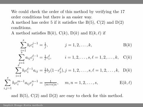
We could check the order of this method by verifying the 17order conditions but there is an easier way.A method has order 5 if it satisfies the B(5), C(2) and D(2)conditions.A method satisfies B(k), C(k), D(k) and E(k, ℓ) if
s∑
i=1
bicj−1i = 1
j, j = 1, 2, . . . , k, B(k)
s∑
j=1
aijcℓ−1j = 1
ℓcℓi , i = 1, 2, . . . , s, ℓ = 1, 2, . . . , k, C(k)
s∑
i=1
bicℓ−1i aij = 1
ℓbj(1−cℓ
j), j = 1, 2, . . . , s, ℓ = 1, 2, . . . , k, D(k)
s∑
i,j=1
bicm−1i aijc
n−1j = 1
(m+n)n , m, n = 1, 2, . . . , s, E(k, ℓ)
and B(5), C(2) and D(2) are easy to check for this method.
Implicit Runge–Kutta methods
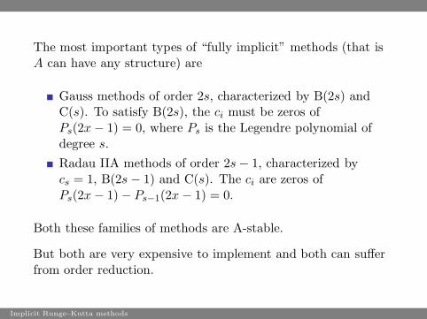
The most important types of “fully implicit” methods (that isA can have any structure) are
Gauss methods of order 2s, characterized by B(2s) andC(s). To satisfy B(2s), the ci must be zeros ofPs(2x − 1) = 0, where Ps is the Legendre polynomial ofdegree s.
Radau IIA methods of order 2s − 1, characterized bycs = 1, B(2s − 1) and C(s). The ci are zeros ofPs(2x − 1) − Ps−1(2x − 1) = 0.
Both these families of methods are A-stable.
But both are very expensive to implement and both can sufferfrom order reduction.
Implicit Runge–Kutta methods
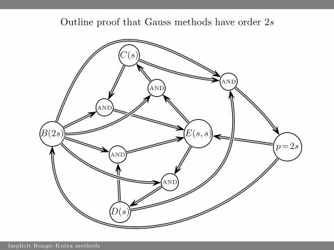
Outline proof that Gauss methods have order 2s
B(2s)
C(s)
D(s)
E(s, s)
p=2s
AND
AND
AND
AND
AND
Implicit Runge–Kutta methods
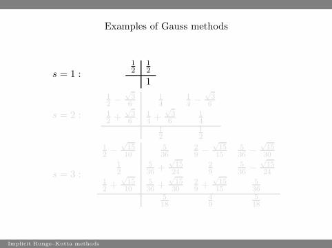
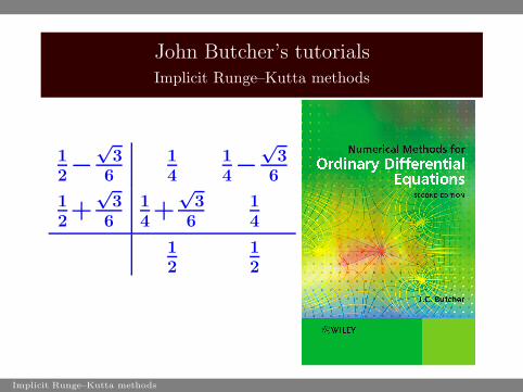
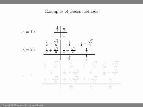
Examples of Gauss methods
s = 1 :12
12
1
s = 2 :
12 −
√
36
14
14 −
√
36
12 +
√
36
14 +
√
36
14
12
12
s = 3 :
12 −
√
1510
536
29 −
√
1515
536 −
√
1530
12
536 +
√
1524
29
536 −
√
1524
12 +
√
1510
536 +
√
1530
29 +
√
1515
536
518
49
518
Implicit Runge–Kutta methods
Examples of Gauss methods
s = 1 :12
12
1
s = 2 :
12 −
√
36
14
14 −
√
36
12 +
√
36
14 +
√
36
14
12
12
s = 3 :
12 −
√
1510
536
29 −
√
1515
536 −
√
1530
12
536 +
√
1524
29
536 −
√
1524
12 +
√
1510
536 +
√
1530
29 +
√
1515
536
518
49
518
Implicit Runge–Kutta methods

Examples of Gauss methods
s = 1 :12
12
1
s = 2 :
12 −
√
36
14
14 −
√
36
12 +
√
36
14 +
√
36
14
12
12
s = 3 :
12 −
√
1510
536
29 −
√
1515
536 −
√
1530
12
536 +
√
1524
29
536 −
√
1524
12 +
√
1510
536 +
√
1530
29 +
√
1515
536
518
49
518
Implicit Runge–Kutta methods
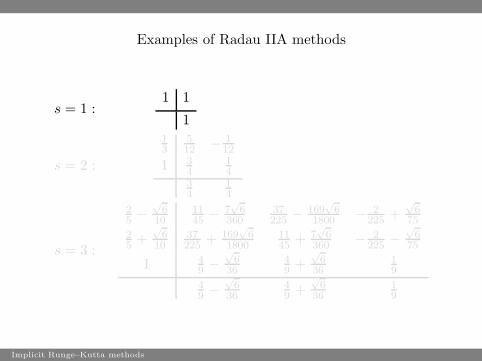
Examples of Radau IIA methods
s = 1 :1 1
1
s = 2 :
13
512 − 1
12
1 34
14
34
14
s = 3 :
25 −
√
610
1145 − 7
√
6360
37225 − 169
√
61800 − 2
225 +√
675
25 +
√
610
37225 + 169
√
61800
1145 + 7
√
6360 − 2
225 −√
675
1 49 −
√
636
49 +
√
636
19
49 −
√
636
49 +
√
636
19
Implicit Runge–Kutta methods
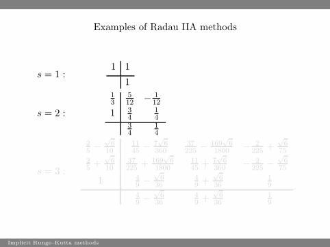
Examples of Radau IIA methods
s = 1 :1 1
1
s = 2 :
13
512 − 1
12
1 34
14
34
14
s = 3 :
25 −
√
610
1145 − 7
√
6360
37225 − 169
√
61800 − 2
225 +√
675
25 +
√
610
37225 + 169
√
61800
1145 + 7
√
6360 − 2
225 −√
675
1 49 −
√
636
49 +
√
636
19
49 −
√
636
49 +
√
636
19
Implicit Runge–Kutta methods
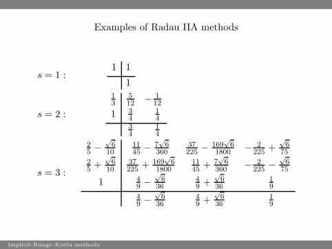
Examples of Radau IIA methods
s = 1 :1 1
1
s = 2 :
13
512 − 1
12
1 34
14
34
14
s = 3 :
25 −
√
610
1145 − 7
√
6360
37225 − 169
√
61800 − 2
225 +√
675
25 +
√
610
37225 + 169
√
61800
1145 + 7
√
6360 − 2
225 −√
675
1 49 −
√
636
49 +
√
636
19
49 −
√
636
49 +
√
636
19
Implicit Runge–Kutta methods
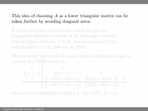
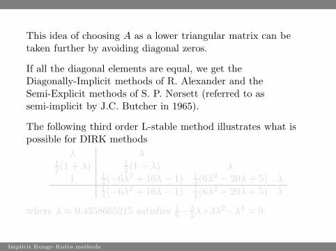
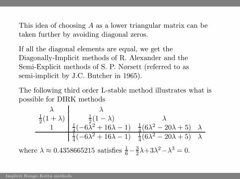
This idea of choosing A as a lower triangular matrix can betaken further by avoiding diagonal zeros.
If all the diagonal elements are equal, we get theDiagonally-Implicit methods of R. Alexander and theSemi-Explicit methods of S. P. Nørsett (referred to assemi-implicit by J.C. Butcher in 1965).
The following third order L-stable method illustrates what ispossible for DIRK methods
λ λ12(1 + λ) 1
2(1 − λ) λ1 1
4(−6λ2 + 16λ − 1) 14(6λ2 − 20λ + 5) λ
14(−6λ2 + 16λ − 1) 1
4(6λ2 − 20λ + 5) λ
where λ ≈ 0.4358665215 satisfies 16−
32λ+3λ2−λ3 = 0.
Implicit Runge–Kutta methods
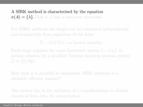
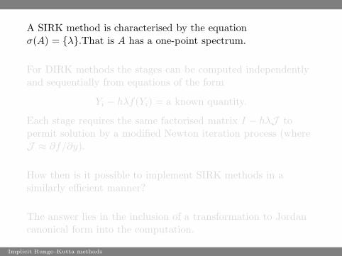
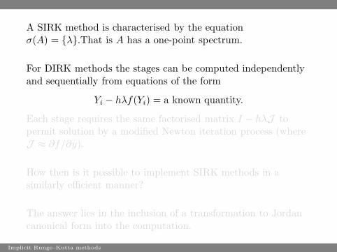
A SIRK method is characterised by the equationσ(A) = {λ}.That is A has a one-point spectrum.
For DIRK methods the stages can be computed independentlyand sequentially from equations of the form
Yi − hλf(Yi) = a known quantity.
Each stage requires the same factorised matrix I − hλJ topermit solution by a modified Newton iteration process (whereJ ≈ ∂f/∂y).
How then is it possible to implement SIRK methods in asimilarly efficient manner?
The answer lies in the inclusion of a transformation to Jordancanonical form into the computation.
Implicit Runge–Kutta methods
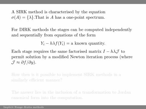
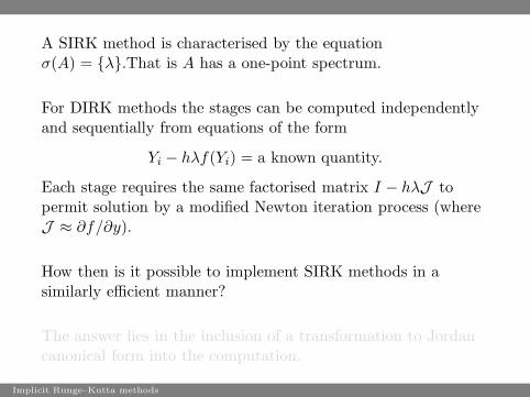
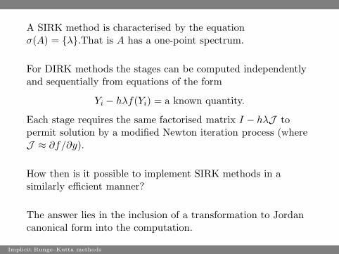
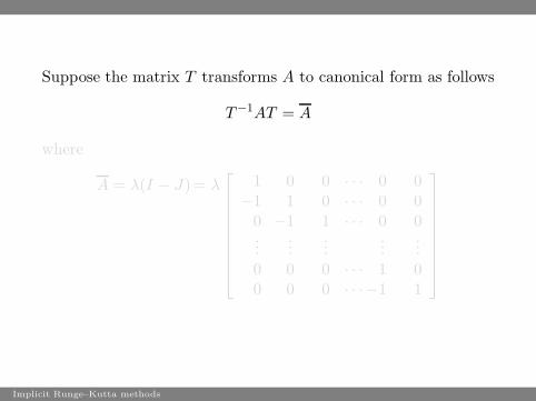
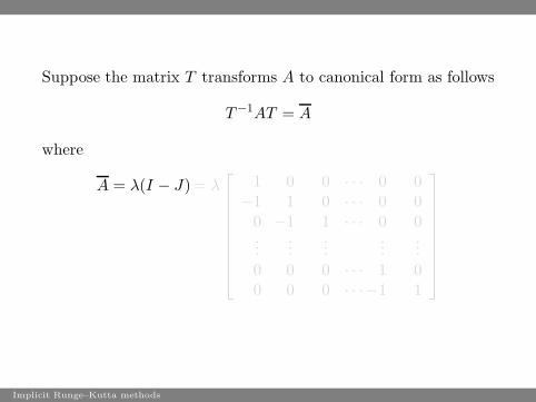
Suppose the matrix T transforms A to canonical form as follows
T−1AT = A
where
A = λ(I − J)= λ
1 0 0 · · · 0 0−1 1 0 · · · 0 0
0 −1 1 · · · 0 0...
......
......
0 0 0 · · · 1 00 0 0 · · · −1 1
Implicit Runge–Kutta methods
Suppose the matrix T transforms A to canonical form as follows
T−1AT = A
where
A = λ(I − J)= λ
1 0 0 · · · 0 0−1 1 0 · · · 0 0
0 −1 1 · · · 0 0...
......
......
0 0 0 · · · 1 00 0 0 · · · −1 1
Implicit Runge–Kutta methods

Suppose the matrix T transforms A to canonical form as follows
T−1AT = A
where
A = λ(I − J)= λ
1 0 0 · · · 0 0−1 1 0 · · · 0 0
0 −1 1 · · · 0 0...
......
......
0 0 0 · · · 1 00 0 0 · · · −1 1
Implicit Runge–Kutta methods
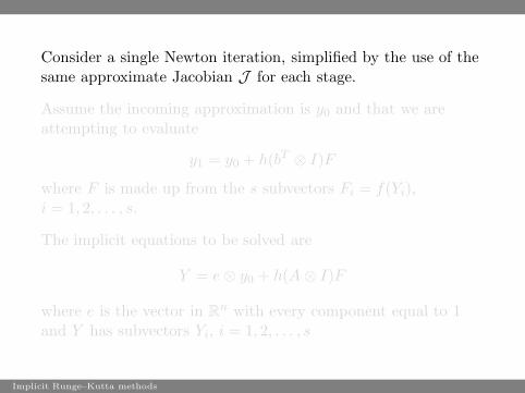
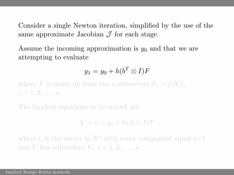
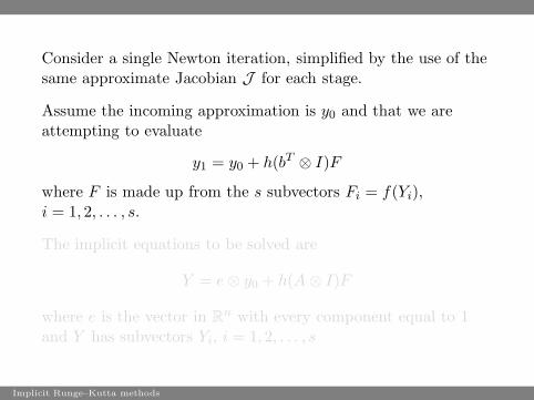
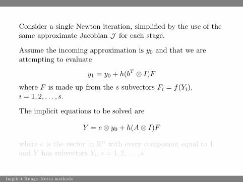
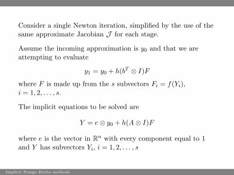
Consider a single Newton iteration, simplified by the use of thesame approximate Jacobian J for each stage.
Assume the incoming approximation is y0 and that we areattempting to evaluate
y1 = y0 + h(bT ⊗ I)F
where F is made up from the s subvectors Fi = f(Yi),i = 1, 2, . . . , s.
The implicit equations to be solved are
Y = e ⊗ y0 + h(A ⊗ I)F
where e is the vector in Rn with every component equal to 1
and Y has subvectors Yi, i = 1, 2, . . . , s
Implicit Runge–Kutta methods

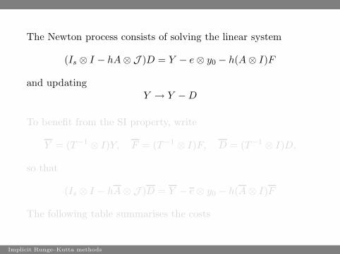
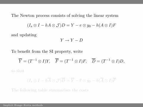
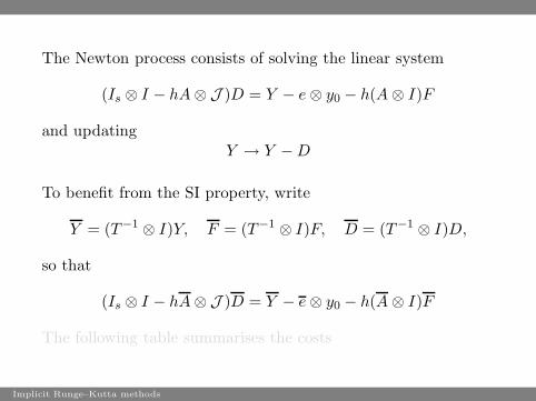
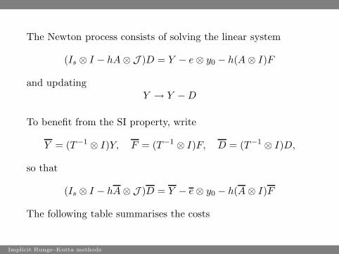
The Newton process consists of solving the linear system
(Is ⊗ I − hA ⊗ J )D = Y − e ⊗ y0 − h(A ⊗ I)F
and updatingY → Y − D
To benefit from the SI property, write
Y = (T−1 ⊗ I)Y, F = (T−1 ⊗ I)F, D = (T−1 ⊗ I)D,
so that
(Is ⊗ I − hA ⊗ J )D = Y − e ⊗ y0 − h(A ⊗ I)F
The following table summarises the costs
Implicit Runge–Kutta methods
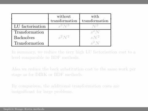
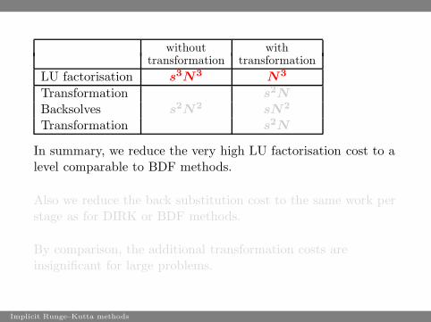
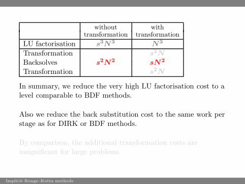
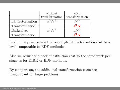
without withtransformation transformation
LU factorisation s3N
3N
3
Transformation s2N
Backsolves s2N
2sN
2
Transformation s2N
In summary, we reduce the very high LU factorisation cost to alevel comparable to BDF methods.
Also we reduce the back substitution cost to the same work perstage as for DIRK or BDF methods.
By comparison, the additional transformation costs areinsignificant for large problems.
Implicit Runge–Kutta methods
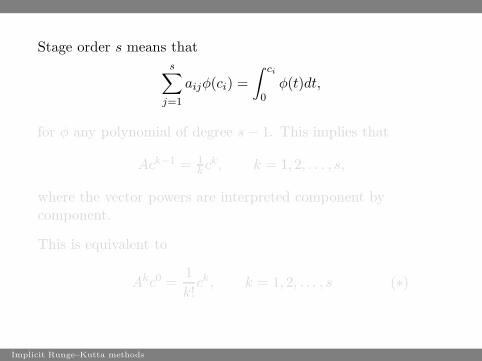
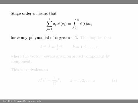
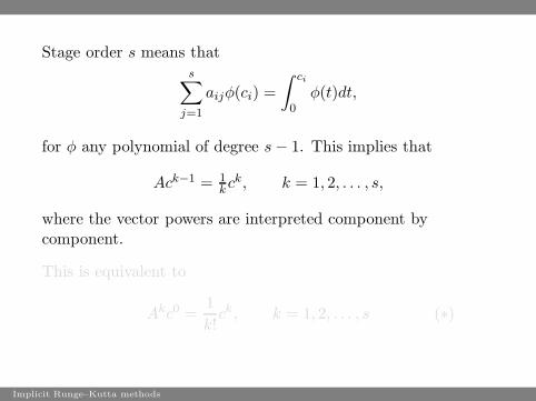
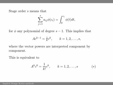
Stage order s means thats∑
j=1
aijφ(ci) =
∫ ci
0φ(t)dt,
for φ any polynomial of degree s − 1. This implies that
Ack−1 = 1kck, k = 1, 2, . . . , s,
where the vector powers are interpreted component bycomponent.
This is equivalent to
Akc0 =1
k!ck, k = 1, 2, . . . , s (∗)
Implicit Runge–Kutta methods
Stage order s means thats∑
j=1
aijφ(ci) =
∫ ci
0φ(t)dt,
for φ any polynomial of degree s − 1. This implies that
Ack−1 = 1kck, k = 1, 2, . . . , s,
where the vector powers are interpreted component bycomponent.
This is equivalent to
Akc0 =1
k!ck, k = 1, 2, . . . , s (∗)
Implicit Runge–Kutta methods

Stage order s means thats∑
j=1
aijφ(ci) =
∫ ci
0φ(t)dt,
for φ any polynomial of degree s − 1. This implies that
Ack−1 = 1kck, k = 1, 2, . . . , s,
where the vector powers are interpreted component bycomponent.
This is equivalent to
Akc0 =1
k!ck, k = 1, 2, . . . , s (∗)
Implicit Runge–Kutta methods
Stage order s means thats∑
j=1
aijφ(ci) =
∫ ci
0φ(t)dt,
for φ any polynomial of degree s − 1. This implies that
Ack−1 = 1kck, k = 1, 2, . . . , s,
where the vector powers are interpreted component bycomponent.
This is equivalent to
Akc0 =1
k!ck, k = 1, 2, . . . , s (∗)
Implicit Runge–Kutta methods
Stage order s means thats∑
j=1
aijφ(ci) =
∫ ci
0φ(t)dt,
for φ any polynomial of degree s − 1. This implies that
Ack−1 = 1kck, k = 1, 2, . . . , s,
where the vector powers are interpreted component bycomponent.
This is equivalent to
Akc0 =1
k!ck, k = 1, 2, . . . , s (∗)
Implicit Runge–Kutta methods
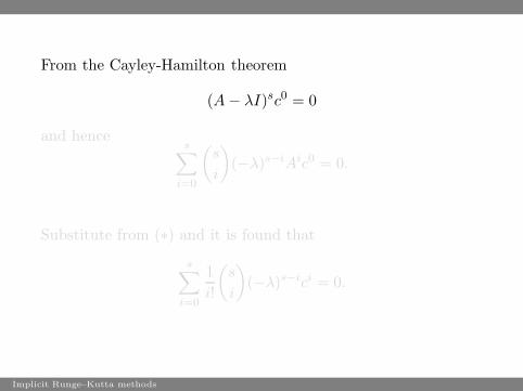
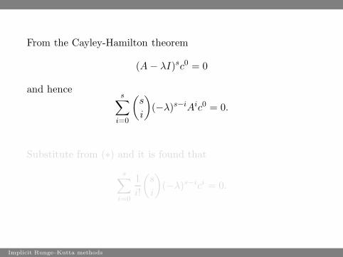
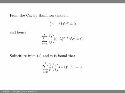
From the Cayley-Hamilton theorem
(A − λI)sc0 = 0
and hences∑
i=0
(s
i
)(−λ)s−iAic0 = 0.
Substitute from (∗) and it is found that
s∑
i=0
1
i!
(s
i
)(−λ)s−ici = 0.
Implicit Runge–Kutta methods
From the Cayley-Hamilton theorem
(A − λI)sc0 = 0
and hences∑
i=0
(s
i
)(−λ)s−iAic0 = 0.
Substitute from (∗) and it is found that
s∑
i=0
1
i!
(s
i
)(−λ)s−ici = 0.
Implicit Runge–Kutta methods
From the Cayley-Hamilton theorem
(A − λI)sc0 = 0
and hences∑
i=0
(s
i
)(−λ)s−iAic0 = 0.
Substitute from (∗) and it is found that
s∑
i=0
1
i!
(s
i
)(−λ)s−ici = 0.
Implicit Runge–Kutta methods
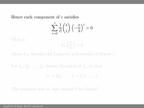
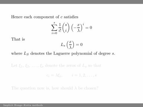
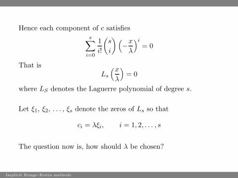
Hence each component of c satisfiess∑
i=0
1
i!
(s
i
) (−
x
λ
)i
= 0
That isLs
(x
λ
)= 0
where LS denotes the Laguerre polynomial of degree s.
Let ξ1, ξ2, . . . , ξs denote the zeros of Ls so that
ci = λξi, i = 1, 2, . . . , s
The question now is, how should λ be chosen?
Implicit Runge–Kutta methods
Hence each component of c satisfiess∑
i=0
1
i!
(s
i
) (−
x
λ
)i
= 0
That isLs
(x
λ
)= 0
where LS denotes the Laguerre polynomial of degree s.
Let ξ1, ξ2, . . . , ξs denote the zeros of Ls so that
ci = λξi, i = 1, 2, . . . , s
The question now is, how should λ be chosen?
Implicit Runge–Kutta methods

Hence each component of c satisfiess∑
i=0
1
i!
(s
i
) (−
x
λ
)i
= 0
That isLs
(x
λ
)= 0
where LS denotes the Laguerre polynomial of degree s.
Let ξ1, ξ2, . . . , ξs denote the zeros of Ls so that
ci = λξi, i = 1, 2, . . . , s
The question now is, how should λ be chosen?
Implicit Runge–Kutta methods
Hence each component of c satisfiess∑
i=0
1
i!
(s
i
) (−
x
λ
)i
= 0
That isLs
(x
λ
)= 0
where LS denotes the Laguerre polynomial of degree s.
Let ξ1, ξ2, . . . , ξs denote the zeros of Ls so that
ci = λξi, i = 1, 2, . . . , s
The question now is, how should λ be chosen?
Implicit Runge–Kutta methods
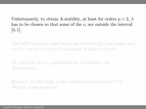
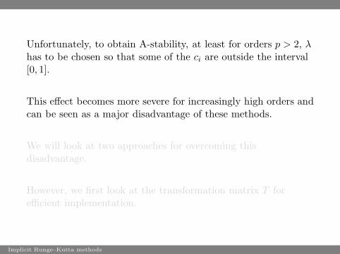
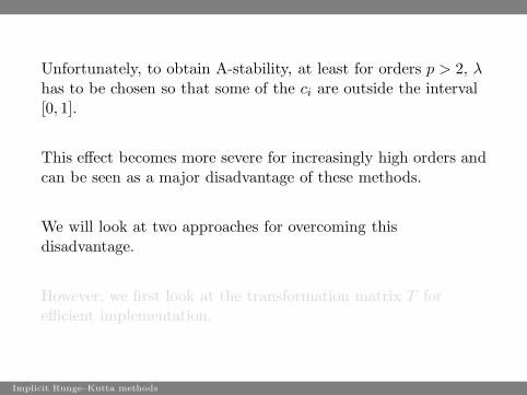
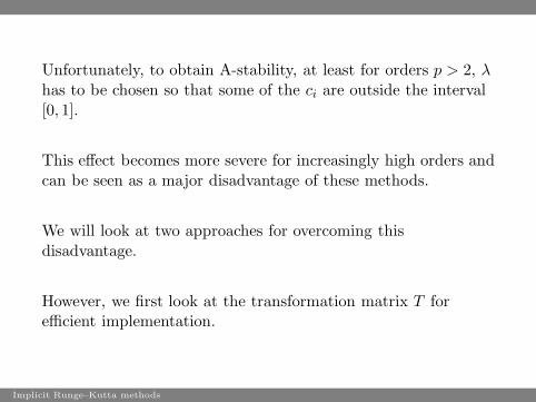
Unfortunately, to obtain A-stability, at least for orders p > 2, λhas to be chosen so that some of the ci are outside the interval[0, 1].
This effect becomes more severe for increasingly high orders andcan be seen as a major disadvantage of these methods.
We will look at two approaches for overcoming thisdisadvantage.
However, we first look at the transformation matrix T forefficient implementation.
Implicit Runge–Kutta methods
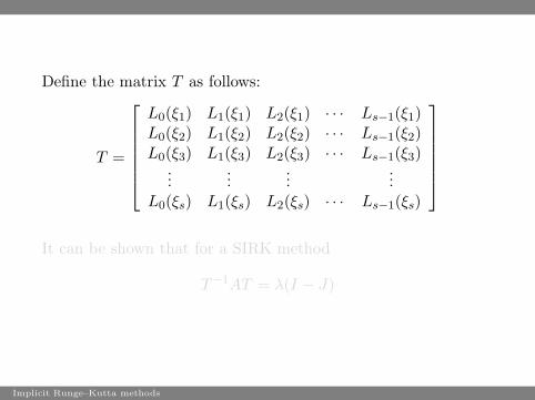
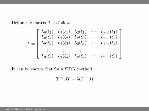
Define the matrix T as follows:
T =
L0(ξ1) L1(ξ1) L2(ξ1) · · · Ls−1(ξ1)L0(ξ2) L1(ξ2) L2(ξ2) · · · Ls−1(ξ2)L0(ξ3) L1(ξ3) L2(ξ3) · · · Ls−1(ξ3)
......
......
L0(ξs) L1(ξs) L2(ξs) · · · Ls−1(ξs)
It can be shown that for a SIRK method
T−1AT = λ(I − J)
Implicit Runge–Kutta methods
Define the matrix T as follows:
T =
L0(ξ1) L1(ξ1) L2(ξ1) · · · Ls−1(ξ1)L0(ξ2) L1(ξ2) L2(ξ2) · · · Ls−1(ξ2)L0(ξ3) L1(ξ3) L2(ξ3) · · · Ls−1(ξ3)
......
......
L0(ξs) L1(ξs) L2(ξs) · · · Ls−1(ξs)
It can be shown that for a SIRK method
T−1AT = λ(I − J)
Implicit Runge–Kutta methods
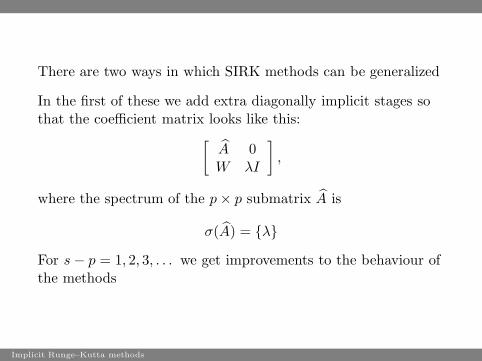
There are two ways in which SIRK methods can be generalized
In the first of these we add extra diagonally implicit stages sothat the coefficient matrix looks like this:
[A 0W λI
],
where the spectrum of the p × p submatrix A is
σ(A) = {λ}
For s − p = 1, 2, 3, . . . we get improvements to the behaviour ofthe methods
Implicit Runge–Kutta methods

A second generalization is to replace “order” by “effectiveorder”.
This allows us to locate the abscissae where we wish.
In “DESIRE” methods:
Diagonally Extended Singly Implicit Runge-Kutta methodsusing Effective order
these two generalizations are combined.
This seems to be as far as we can go in constructing efficientand accurate singly-implicit Runge-Kutta methods.
Implicit Runge–Kutta methods