Joint optimal train regulation and passenger flow control strategy forhigh-frequency metro lines

Shukai Lia,∗, Maged M. Dessoukyb, Lixing Yanga,∗, Ziyou Gaoa

aState Key Laboratory of Rail Traffic Control and Safety, Beijing Jiaotong University, Beijing, 100044, ChinabThe Daniel J. Epstein Department of Industrial and Systems Engineering, University of Southern California, Los Angeles,

CA 90089-0193, USA

Abstract

To improve the headway regularity and commercial speed of high-frequency metro lines with overloaded

passenger flow, this paper systematically investigates a joint optimal dynamic train regulation and passenger

flow control design for metro lines. A coupled state-space model for the evolution of the departure time and

the passenger load of each train at each station is explicitly developed. The dwell time of the train is affected

by the number of entering and exiting passengers. Combining dynamic train regulation and passenger flow

control, a dynamic optimisation problem that minimises the timetable and the headway deviations for metro

lines is developed. By applying a model predictive control (MPC) method, we formulate the problem of

finding the optimal joint train regulation and passenger flow control strategy as the problem of solving a set

of quadratic programming (QP) problems, under which an optimal control law can be numerically calculated

efficiently using a quadratic programming algorithm. Moreover, based on the Lyapunov stability theory, the

stability (convergence) of the metro line system under the proposed optimal control algorithm is verified.

Numerical examples are given to illustrate the effectiveness of the proposed method.

Keywords: Train regulation, Passenger flow control, Quadratic programming, System stability

1. Introduction

1.1. Motivation

Urban metro transportation systems have became a rapid, clean, efficient way to transport passengers

in many modern large cities for relieving the traffic pressure. Different to traditional passenger railway

traffic, metro line systems have inherent features of high frequency and traffic density, which can lead to

instability of this transportation system. Any deviation with respect to the nominal schedule of a given train

is amplified with time due to the accumulation of passengers, which is similar to the familiar bus bunching

problem in which the accumulation of passengers also leads to the instability of the bus system (Daganzo,

2009; Daganzo and Pilachowski, 2011; Sanchez-Martınez et al., 2016). If an inevitable disturbance happens

on the metro line system, such as equipment failure or inadequate driver/passenger actions, the train will

be delayed and train delays will increase from one station to the next with the accumulation of passengers,

so that the whole metro line system operation will be affected. In order to restore the disturbed traffic to

an acceptable situation for metro lines, train regulation manipulating the running time and the dwell time

∗Corresponding authors. Tel.: +86 18201061093.Email addresses: shkli@bjtu.edu.cn (Shukai Li), lxyang@bjtu.edu.cn (Lixing Yang)

Preprint submitted to Elsevier January 19, 2017

of each train is therefore necessary to recover train delays and to prevent the instability of the metro line

operation.

With increasing urbanization, the increasing population and economic activities create a significant rise

for the demand of metro transportation systems. Typically, the passenger arrival flow is extremely large

during the peak hours of the workday. For example, a survey of the Beijing metro line system shows that

the overloaded passenger count of the trains usually exceeds 120% during peak hours, causing a number of

stations to adopt measures to control the passenger arrival flow. The dwell time of the train at the station

depends on the number of passengers arriving to the station. The high passenger arrival flow during the

peak hours magnifies the dwell time of the train and leads to train delays, especially under the case of a

disturbance event occurring. The overloaded passenger flow aggravates the instability of metro lines and

further affects the operational efficiency of the metro lines. Therefore, for the peak hours of the workday,

it is essential to investigate how to control the large passenger arrival rate, apart from conducting train

regulation to recover train delays from disturbed situations.

Since metro-type rail lines operate according to a given timetable, the main goal of regulation is a

full timetable recovery to improve the commercial speed (the total traveling speed), while maintaining the

regularity of the headway to minimize the accumulation of passengers and reduce undue passenger waiting

time (Fernandez et al., 2006). The regulation of metro lines seeks a compromise between timetable and

headway deviations during the transient period. Based on this, the research scope of this paper is a full

timetable recovery from train delays under disturbances in a certain range, and the aim is to determine

the joint dynamic train regulation and passenger flow control strategy by taking into consideration the

overloaded passenger flow, providing the system with flexibility for recovery from disturbed situations, so as

to ensure the stability and improve the headway regularity and commercial speed of the metro line system.

1.2. Literature review

As an important transportation mode in a modern metropolis, the metro line system has attracted sub-

stantial attention by researchers over the last decades. The literature on the metro line system includes two

main categories: train timetabling ( train schedules) and train rescheduling problems. The train timetabling

problem aims to determine a pre-operation schedule for a set of trains for the metro line system, while the

target of the train rescheduling process is to cope with the unpredicted events and the train rescheduling

model needs to adjust the current timetable in an effective way when a disturbance occurs.

To study the train timetabling problem of a metro line system, the early work of Cury et al. (1980)

proposed an analytical model with two dynamic equations: the headway and the passenger equations, and

established a cost function that includes passenger delay, passenger comfort, and efficient train operation.

The generation of optimal schedules for metro lines was formulated as a nonlinear dynamic programming

problem, and solved by an iterative hierarchical multilevel decomposition method. Minciardi et al. (1995)

dealt with the problem of generating daily train schedules for an underground railway line, which opti-

mized the quality of the service expressed as the mean time spent by the passengers in the system with

the safety constraints on the motion of trains. To improve the computational efficiency, Assis and Milani

(2004) proposed a new methodology for computing the optimal train schedules for metro lines using a linear-

programming-based model predictive control formulation. The proposed methodology is computationally

efficient and can generate optimal schedules for a whole day operation as well as schedules for transitions

between two separate time periods with known schedules. Mannino and Mascis (2009) discussed a number

of theoretical and practical results related to the implementation of an exact algorithm to route and sched-

2

ule trains in real time for metro stations. Niu and Zhou (2013) focused on optimizing a passenger train

timetable in a heavily congested urban rail corridor, and developed a nonlinear optimization model to solve

the problem on practical sized corridors subject to the available train-unit fleet. Sun et al. (2014) formulated

three optimization models to design demand-sensitive timetables for metro services by representing train

operations using equivalent time. Li and Hong (2014) formulated an integrated energy-efficient operation

model to optimize the timetable and speed profile for metro line operations. Niu et al. (2015) developed

train schedules to minimize the total passenger waiting time using a nonlinear integer programming model

with linear constraints. Yang et al. (2016) developed a two-stage stochastic integer programming model

to minimize the expected travel time and penalty value incurred by transfer activities for metro networks.

Das Gupta et al. (2016) proposed a two-step linear optimization model to calculate energy-efficient timeta-

bles for metro railway networks. Yin et al. (2017) designed a dynamic passenger demand oriented metro

train scheduling to minimize the energy consumption and waiting time by using a mixed-integer linear

programming approach.

In case a disturbance or a disruption occurs in the metro line, the optimized train timetables are not able

to keep the original optimized objectives. The train rescheduling process has to be initiated to recover train

delays and reduce the effect of the unpredicted events (Chang and Chung, 2005; Corman et al., 2012; Dundar

and Sahin, 2013; Cacchiani et al., 2014; Veelenturf et al., 2016). Usually, for the general railway system with

the larger travel time, the train operation strategies, such as overtaking, meeting and crossing are allowable

to implement for improving rescheduling efficiency. However, these strategies are commonly prohibited in an

urban metro system with the smaller travel time, where the trains have the same priority, and the overtaking

between train is not allowed for metro lines (Van Breusegem et al., 1991; Niu et al., 2015; Yin et al., 2016).

In addition, the metro train rescheduling should particularly consider the passengers’ influencing factors

(Van Breusegem et al., 1991; Yin et al., 2016). The methods for the general railway rescheduling are usually

infeasible for metro train rescheduling problems.

In particular, there are two rescheduling approaches for an urban metro system, where one is to recover

the original timetable, and another is to redesign a new train scheduling plan. Every day small or slight

delays occur in almost all the urban metro lines, and the affected trains need several stations to compensate

for the delays, then a transient period is needed to reach the nominal timetable. In this case, the train

regulation strategy by dynamically adjusting the running time and the dwell time of each train is applied

to recover the original timetable from disturbances (Fernandez et al., 2006; Lin and Sheu, 2010). The

corresponding train rescheduling is also called Automatic Train Regulation (ATR), which is a core function

of modern metro signalling systems and plays an important role in maintaining schedule and headway

adherence. The train regulation strategy is an on-line and dynamic rescheduling approach, which is based

on real-time feedback information and generates the train rescheduling strategy in real-time. On the other

hand, in the presence of large delays, if the duration of the regulation transient and the magnitude of time

deviations from the nominal timetable are unacceptable, then a rescheduling process is needed, and a new

delayed nominal timetable could be established, which is an off-line rescheduling approach with the real-time

requirement for the algorithm design (Corman et al., 2012; Dundar and Sahin, 2013; Yin et al., 2016). For

the above two rescheduling approaches, this paper focuses on the first case to recover the original timetable

from disturbances.

Usually, the buffer times or supplements in the timetable are designed to absorb the train delays re-

sulting from disturbances (Vansteenwegen and Oudheusden, 2004; Abril et al., 2008). However, buffer

time allocations are static and cannot be used dynamically and flexibly from a system-wide point of view,

3

which may reduce the system utilization. Moreover, online train regulation can be applied to recover the

schedule/headway deviations resulting from disturbances by dynamically adjusting the running time and

the dwell time of each train. Many online train regulation techniques have been proposed for metro lines.

Van Breusegem et al. (1991) proposed a complete discrete-event traffic model of metro lines and designed

a state feedback control algorithm to ensure system stability and the minimization of a given performance

index based on a linear quadratic regulator approach. This model is useful to analyze the stability of a

metro-type traffic regulation. By using a fuzzy expert system approach, Chang and Thia (1996) designed

an online timetable rescheduling of mass rapid transit trains to maintain the quality of train service after

sudden load disturbances. The proposed methodology is fast enough for online implementation. Goodman

and Murata (2001) proposed a classical optimization approach to regulating metro traffic to encapsulate

the travelling passengers perception of the quality of the service provided. In Chang and Chung (2005),

a genetic algorithm was applied to solve the optimal train regulation problem efficiently. Fernandez et al.

(2006) proposed a predictive traffic regulation model for metro loop lines on the basis of the optimization

of a cost function along a time horizon and proposed regulation strategies to minimize the timetable and

headway deviations by modifying the train run times. Lin and Sheu (2010) proposed an automatic train

regulation method using a dual heuristic dynamic program to handle the non-linear and stochastic charac-

teristics of metro lines, and obtained a near-optimal regulation rapidly. Recently, regarding environment

sustainability and energy saving, Sheu and Lin (2012) proposed a dual heuristic programming method for

designing automatic train regulation of a metro line with energy saving by coasting and station dwell time

control, and the evaluation shows that better traffic regulation with higher energy efficiency is attainable.

Kang et al. (2015) proposed a rescheduling model for the last train by considering the train delays caused

by incidents that occurred in urban railway transit networks, and designed a genetic algorithm to minimize

the difference between the original timetable and the rescheduled one. Xu et al. (2016) considered an inci-

dent on a track of a double-track subway line, and formulated an optimization model to find near-optimal

rescheduled timetables with the least total delay time compared to the original one.

Train regulation problems for metro lines are usually formulated as an optimization problem and solved

using nonlinear programming or dynamic programming by combining heuristic algorithms. However, for

large-scale nonlinear optimization problems, the computation time is still long, making the problem in-

tractable in real time. In this paper, we use a model predictive control (MPC) algorithm to efficiently

handle large-scale optimization problems with hard physical constraints, which have been successfully ap-

plied in many large-scale transportation systems (Caimi et al., 2007; Le et al., 2013). For instance, Lin

et al. (2011) applied model predictive control to control and coordinate urban traffic networks, for which

the computation time is significantly reduced. Based on a model predictive control approach, Haddad et al.

(2013) tackled the macroscopic traffic modeling and control of a large-scale mixed transportation network

consisting of a freeway and an urban network, in order to minimize total delay for the entire network. By

considering the uncertain passenger arrival flow, Li et al. (2016) applied model predictive control for train

regulation in underground railways to ensure the minimization of an upper bound on the metro system cost

function, showing that the proposed train regulation has a low online computation burden. This feature

makes the MPC algorithm an ideal candidate for real-time metro traffic regulation.

1.3. Proposed approach and contributions

Note that there are many works on the study of train regulation methods for metro lines, which are

mainly conducted by manipulating the running times and the dwell times of the trains. However, for peak

4

hours with overloaded passengers, train regulation by just manipulating the running time and the dwell

time of each train can not easily handle the overcrowded passenger flow. To the best of our knowledge,

under the case that a disturbance or disruption occurs, few works pay attention to designing the train

regulation by also considering the passenger flow control. Moreover, considering that existing nonlinear

programming and dynamic programming methods become computationally prohibitive to deal with large

optimization problems in real time, other approaches are needed to solve this problem. Based on the above

considerations, this study focuses on the joint dynamic train regulation and passenger flow control design

problem for metro lines to improve the headway regularity and commercial speed.

Specifically, the contributions of this paper are as follows.

(1) The dwell time of each train is affected by both the number of entering and exiting passengers. In

contrast, existing studies usually do not consider passenger flow control in the train regulation problem (Yin

et al., 2016; Li et al., 2016). By considering the sudden large passenger flow for high-frequency metro lines,

this study constructs a coupled dynamic model for the evolution of both the train traffic and the passenger

load, and designs a joint optimal train regulation and passenger flow control strategy. The proposed coupled

dynamic model provides a new and more accurate insight for the train regulation problem.

(2) The proposed on-line optimization algorithm provides a real-time train regulation and passenger

flow control strategy in the form of a closed loop system, which can be effectively and quickly implement-

ed for practical metro lines in real-time. By using Lyapunov stability theory, the stability (convergence)

characteristic of the metro line system has been verified under the proposed optimization algorithm.

The main features of our paper are summarized in Table 1 based on the four characteristics (research

problem, traffic model, solution methodology and stability property) as compared to several related studies.

The rest of this paper is organized as follows. In Section 2, a coupled dynamic model for the evolution

of the departure time and the passenger load of each train is presented. In Section 3, the optimal joint

train regulation and passenger flow control strategy for high-frequency metro lines is designed. In Section

4, numerical examples are provided to demonstrate the effectiveness of the proposed methods. We conclude

this paper in Section 5.

Table 1: The comparison of different characteristics of related models and methods.

Characteristics Research problem Traffic model Solution methodology Stability property

Assis and Milani (2004) Train schedule Train and passenger Linear-programming-based Did not verify system stability

load dynamics Model predictive control

Niu et al. (2015) Train schedule Train dynamics with Nonlinear mixed integer Did not verify system stability

passenger demand programming

Van Breusegem et al. (1991) Train regulation Only train dynamics Linear quadratic regulator Verified system stability

Fernandez et al. (2006) Train regulation Only train dynamics Quadratic programming Did not verify system stability

Lin and Sheu (2010) Train regulation Only train dynamics Dynamic programming Did not verify system stability

Kang et al. (2015) Train regulation Only train dynamics Genetic algorithm Did not verify system stability

Yin et al. (2016) Train regulation Train dynamics with Approximate dynamic Did not verify system stability

passenger demands programming

This paper Train regulation and Train and passenger Quadratic-programming-based Verified system stability

passenger flow control load dynamics Model predictive control

5

2. Problem description

We consider a metro-type railway line with N stations and one terminal station, and an ordered set of

trains are running on the stations and stop at the stations to allow passengers to embark and disembark.

A metro-type railway line system mainly involves stations, trains and passengers. The aim of the operation

management is to ensure the trains can transport all the passengers from their origin station to destination

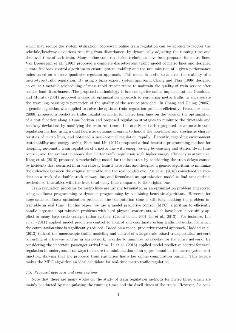
station in a safe and efficient way. An illustration for the operation of a metro-type railway line is shown in

Figure 1.

Table 2: Indices and parameters used throughout the paper.

i = 1, 2, . . . , Z: indices of the trains on the line;

j = 1, 2, . . . , N : indices of the stations on the line;

System Parameters

Rij : the nominal running time of train i from station j to station j + 1;

Dj : the minimal dwell time at a station when no passenger gets on the train;

α: the delay rate for one passenger to get on or off a train;

βij : a disembarking proportionality factor at station j for train i;

γij : the passenger arrival rate to station j for train i;

H: the scheduled headway;

lmax: the maximum passenger load capacity of the train;

State Variables

tij : the actual departure time of the i-th train from the j-th station;

T ij : the nominal departure time of the i-th train from the j-th station;

rij : the running time of the i-th train from the j-th station to the j + 1-th station;

sij : the dwell time of the i-th train at the j-th station;

lij : the actual load of train i between station j and (j + 1);

Lij : the nominal load of train i between station j and (j + 1);

mij : the number of passengers entering train i at station j;

nij : the number of passengers exiting train i at station j;

w1ij : the uncertain disturbance term to the running time;

w2ij+1: the uncertain disturbance term to the dwell time;

T : the considered time horizon;

M : the finite prediction horizon;

Decision Variables

u1ij : the control strategy to magnify the running time;

u2ij : the dwell time adjustment;

pij : the control strategy to magnify the number of passengers.

6

Station 1 Station 2 Station N

Train iTrain k

Train direction

Train k-1 Train i+1

Terminal

Figure 1. The illustration of the metro-type railway line.

In real-time operations of metro lines, disturbances and disruptions are inevitable, such as equipment

failure or inadequate driver/passenger actions, etc. When a disturbance or a disruption occurs, the optimized

train timetable is not able to keep the original optimized objective, and a train regulation process has to

be initiated to reduce train delays and the effect of the unpredicted events. Especially, during the peak

hours of the day, the passenger demands for most of the stations are extremely large. As a result, when

the train arrives at one station, the passenger load of the train is usually over its nominal passenger load.

Under this case, if the passenger arrival flow is not controlled, the surplus passengers will try to get on

the train, which will result in making the train delays even longer, and even worse the surplus passengers

could lead to a potential unsafe environment in the metro line system. Therefore, when trains deviate from

their nominal time schedule under a disturbance or a disruption, it is necessary to consider both the train

regulation strategy and the passenger flow control strategy to improve the safety and efficiency for the metro

line system.

To address this problem, the train traffic dynamics are first constructed, and then the passenger load

dynamics of the train are developed. Moreover, by combining the coupled relationship between the train

traffic dynamics and the passenger load dynamics, the joint train traffic and passenger flow dynamic model

is presented. Compared to the existing studies which used a time-dependent origin-destination (OD) matrix

to represent passenger demands (Niu et al., 2015; Yin et al., 2016), this study applies a dynamic equation

to describe the dynamic evolution of the passenger load of the train from one station to the next, which is

determined by the number of entering and exiting passengers. The number of entering passengers is assumed

to be proportional to the waiting time between successive trains (Fernandez et al., 2006; Lin and Sheu, 2010),

which is time-dependent, and the number of the exiting passengers is assumed to be proportional to the

number of passengers on the train (Eberlein et al., 2001), which is also time-dependent. Throughout this

paper, the symbols and parameters are listed in Table 2.

2.1. The train traffic dynamics

Based on the discrete-event approach proposed by Van Breusegem et al. (1991), we present the train

traffic dynamics according to the operation of high-frequency metro lines. The train traffic dynamics for the

actual departure time of train i from station j + 1 is given as follows.

tij+1 = tij + rij + sij+1, (1)

and the running time of train i from station j to j + 1 is presented as

rij = Rij + u1

ij + w1

ij , (2)

7

where u1ij is the control strategy to magnify the running time of train i between stations j and j+1, which is

applied to increase the running time when u1ij > 0, and decrease the running time when u1

ij < 0. w1

ij is the

uncertain disturbance term to the running time (such as equipment failure or inadequate driver/passenger

action).

Considering the fact that the dwell time of the train is affected by both the number of entering and

exiting passengers, the dwell time sij+1 is modelled as

sij+1 = α(mij+1 + ni

j+1) +Dj+1 + u2ij+1 + w2

ij+1, (3)

where α is the delay rate representing the time necessary for one passenger to get on or off a train, mij+1

and nij+1 are the number of passengers entering and exiting train i at station j + 1, respectively. u2

ij+1 is

the dwell time adjustment on train i at station j + 1, and w2ij+1 is the uncertain disturbance term to the

dwell time.

Then, by combining (1)–(3), the state-space model for the train traffic dynamics is described by

tij+1 = tij +Rij + α(mi

j+1 + nij+1) +Dj+1 + ui

j + wij , (4)

where uij = u1

ij + u2

ij+1 and wi

j = w1ij + w2

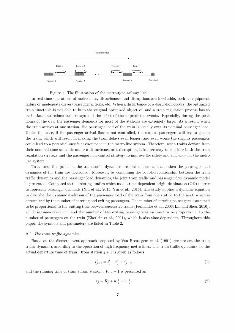
ij+1. An illustration of the train traffic dynamics for a metro

line is plotted in Figure 2, where Figure 2(a) is the case without train regulation and Figure 2(b) is the

case with train regulation. The dotted line represents the nominal timetable, and the solid line denotes the

actual train timetable.

From Figure 2(a), we can find that when the disturbance occurs for the running time of train i − 1 at

station j, train i− 1 is delayed when arriving at station j + 1. At the same time, due to the delay of train

i− 1, the number of arriving passengers is increased, and the train delay increases at station j + 1 with the

accumulation of passengers. Furthermore, by the headway safety constraints, the next train i is also delayed

from station j to station j+1. The train delay increases from one station to the next with the accumulation

of passengers, which shows the instability of the metro line system. So it is necessary to implement train

regulation to recover from the train delays and prevent the instability of the metro line operation. From

Figure 2(b), we can observe that under the train regulation strategy, by adjusting the running time and the

dwell time of train i − 1, and furthermore controlling the passenger arrival flow, the delay of train i − 1 is

effectively reduced, and the delay of train i is also reduced and recovered to the nominal timetable at station

j + 1.

8

Station j

Station j+1

Train i-1

-1i

jt

-1

+1

i

jt

-1 -1

1 i i

j jR w

-1 -1 -1

1 1 1 2 1( ) ! ! ! !! ! !

i i i

j j j jm n D w

Train i

1 i i

j jR w

1 1 1 2 1( ) ! ! ! !! ! !

i i i

j j j jm n D w

i

jt

+1

i

jt

Station j

Station j+1

Train i-1

-1i

jt

-1

+1

i

jt

Train i

i

jt

+1

i

jt

-1 -1 -1

1 1 i i i

j j jR u w

-1 -1 -1 -1

1 1 1 2 1 2 1( ) ! ! ! ! !! ! ! !

i i i i

j j j j jm n D u w

1 1 i i i

j j jR u w

1 1 1 2 1 2 1( ) ! ! ! ! !! ! ! !

i i i i

j j j j jm n D u w

Figure 2. An illustration of the train traffic dynamics.

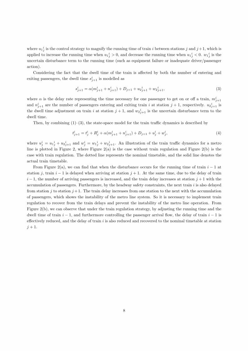
2.2. The passenger load dynamics

When the train arrives at the station, there are passengers entering the train and passengers exiting the

train. Then the dynamic evolution of the passenger load of the train at the station is given by

lij+1 = lij +mij+1 − ni

j+1 + pij+1. (5)

where pij+1 is the control strategy to magnify the number of passengers entering train i at station j + 1,

which is implemented during rush hour or on a special holiday for the sudden gathering of passengers, and

thus is a non-positive value to reduce the passenger load. Under the control strategy for the passenger flow,

the actual number of passengers entering the train is changed to mij+1 + pij+1. In addition, the passenger

load dynamic is mainly determined by the number of entering and exiting passengers and not affected by

the external disturbance.

The number of entering passengers mij+1 is assumed to be proportional to the waiting time between

successive trains, which is given as

mij+1 = γi

j+1(tij+1 − ti−1

j+1), (6)

where γij+1 represents the passengers arrival rate, which can be measured in real time by the monitoring

techniques (Fernandez et al., 2006). Here it should be pointed out that if the number of entering passengers

9

is large and results in an overload of the train, the control strategy pij+1 is conducted to reduce the number

of entering passengers to satisfy the limited capacity of the train for carrying passengers. In particular, with

the control strategy for the passenger flow, the actual dwell time sij+1 is changed to

sij+1 = α(mij+1 + ni

j+1 + pij+1) +Dj+1 + u2ij+1 + w2

ij+1, (7)

which shows the control strategy for the passenger flow not only adjusting the number of passengers entering

the train, but also changing the dwell time of the train. Moreover, we assume that the train stops at each

station. The state constraint for the passenger load is considered to satisfy the requirement of the maximum

capacity of the train, and the control constraint for the running time adjustment u1ij and dwell time

adjustment u2ij is considered to ensure that the final dwell time is larger than the minimum required dwell

time Dj and meanwhile the speed constraint is satisfied for the running time adjustment.

The number of exiting passengers is assumed to be proportional to the number of passengers in the train.

That is, the number of exiting passengers is equal to

nij+1 = βi

j+1lij (8)

where lij is the load of train i between station j and j+1, and βij+1 is a proportionality factor that depends

on station j + 1 and on the hour of travel for train i, which is statistically estimated from the passenger

demand OD matrices during the specific time periods of the day, and thereby represents the OD demand

from different OD pairs for each station. In addition, different to the time-dependent OD matrix adopted

in (Niu et al., 2015; Yin et al., 2016), the dynamic equation (5) describes the dynamic evolution of the

passenger load from one station to the next one for each train, which facilitates to design the dynamic

passenger flow control to adjust the overload of the train.

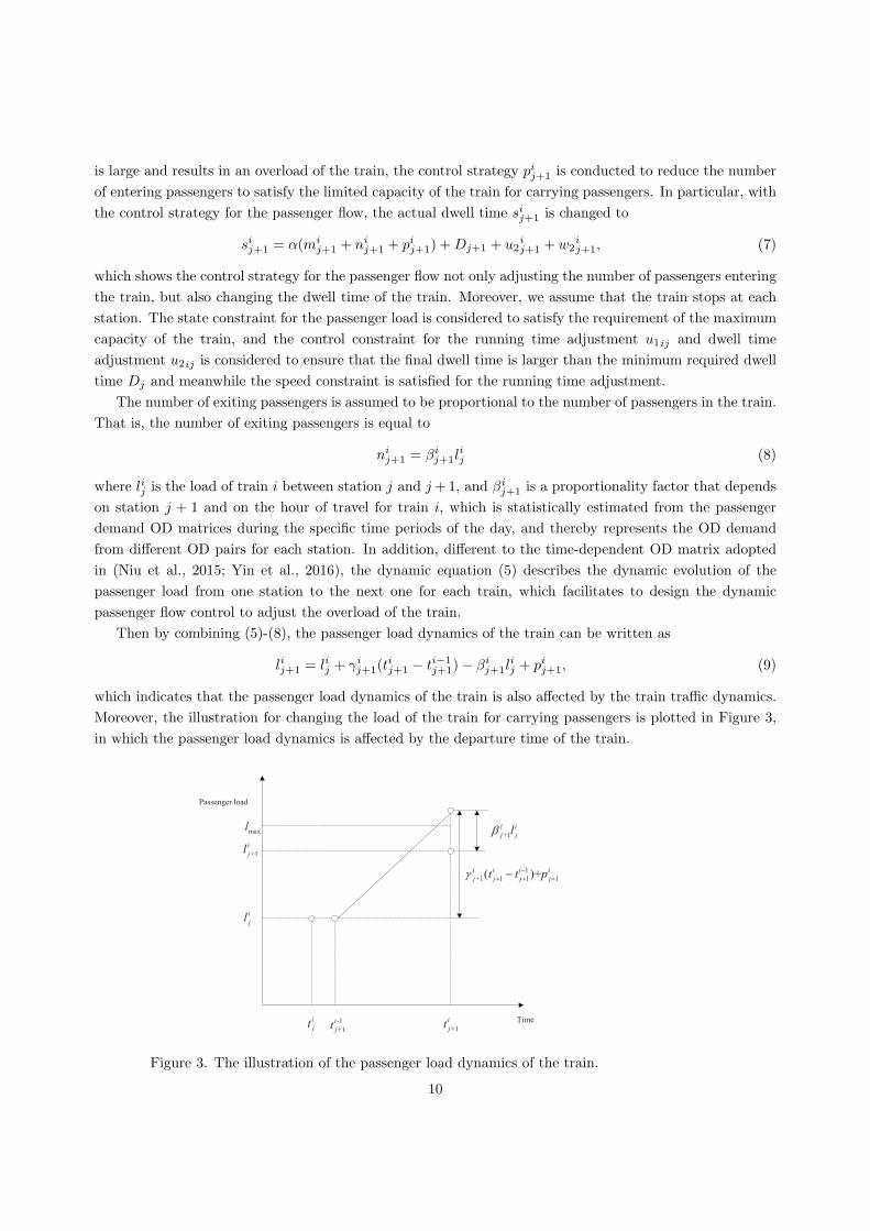
Then by combining (5)-(8), the passenger load dynamics of the train can be written as

lij+1 = lij + γij+1(t

ij+1 − ti−1

j+1)− βij+1l

ij + pij+1, (9)

which indicates that the passenger load dynamics of the train is also affected by the train traffic dynamics.

Moreover, the illustration for changing the load of the train for carrying passengers is plotted in Figure 3,

in which the passenger load dynamics is affected by the departure time of the train.

i

jl

i

jt +1

i

jt

+1

i

jl

-1

+1

i

jtTime

Passenger load

1

+1 1 1 1( )+ !

" " "!

i i i i

j j j jt t p

+1 i i

j jlmaxl

Figure 3. The illustration of the passenger load dynamics of the train.

10

2.3. The joint dynamic model

By combining the above equations (4) and (9), we can obtain the joint dynamic model of the departure

time and the passenger load of the train as follows.{tij+1 = tij +Ri

j + α(γij+1(t

ij+1 − ti−1

j+1) + βij+1l

ij + pij+1) +Dj+1 + ui

j + wij ,

lij+1 = lij + γij+1(t

ij+1 − ti−1

j+1)− βij+1l

ij + pij+1,

(10)

which shows that the departure time and the passenger load of the train influence each other. From equation

(10), we can also observe that if one train is delayed, the train delay increases from one station to the next

station with the accumulation of passengers, which indicates the possible instability of the metro line.

Let xij = [tij , l

ij ]T and ui

j = [uij , p

ij+1]

T . According to equation (10), the joint dynamic model of the

departure time and the passenger load of the train can be obtained together as.

xij+1 = Ai

jxij +Bi

jxi−1j+1 + Ci

j uij +Gi

j(Dj+1 +Rij + wi

j). (11)

where x0j = [0, 0]T , Ai

j =

11−αγi

j+1

αβij+1

1−αγij+1

γij+1

1−αγij+1

1− βij+1 +

αγij+1β

ij+1

1−αγij+1

, Bij =

−αγij+1

1−αγij+1

0

−γij+1

1−αγij+1

0

, Cij =

11−αγi

j+1

α1−αγi

j+1

γij+1

1−αγij+1

11−αγi

j+1

,Gi

j =

11−αγi

j+1

γij+1

1−αγij+1

. The derivation of (11) is given in Appendix A.

The joint dynamic model describes the dynamic changing of the departure time and the passenger load

of the train, which provides a more general model for the operation management of the metro line system

under disturbance or disruption.

It is a common practice to operate with different scheduled headway for different operating hours, e.g.,

peak and off-peak hours. Then for a specific duration of operating hours, a nominal joint traffic and passenger

flow model can be constructed as follows.

T ij+1 = T i

j +Rij + α(γi

j+1(Tij+1 − T i−1

j+1) + βij+1L

ij) +Dj+1 (12)

and

Lij+1 = Li

j + γij+1(T

ij+1 − T i−1

j+1)− βij+1L

ij . (13)

The nominal timetable is characterized by a constant time interval H between two successive trains, i.e.,

H = T ij+1 − T i−1

j+1 . The scheduled headway H of the corresponding operating hours is determined by the

service operating requirement, capacity of the train and passenger flow of the operating hours. In particular,

the scheduled headway H is smaller during the peak hours.

Moreover, to improve the headway regularity and commercial speed, we define the error vector as eij =

[tij −T ij , l

ij −Li

j ]T . According to (12)-(13), together with (11), we can obtain the error dynamics for the joint

dynamic model as follows.

eij+1 = Aije

ij +Bi

jei−1j+1 + Ci

j uij +Gi

jwij . (14)

where Aij , Bi

j , Cij , and Gi

j take the same forms as in (11). The derivation of (14) is given in Appendix B.

Remark 2.1. For the error dynamics (14), noting that eij represents the deviations of the actual departure

time of the train from the nominal departure time and the actual passenger load of the train from the nominal

11

passenger load, then the minimization of ∥eij∥ means to improve the operational efficiency of the metro line

for recovering train delays from disturbances. Moreover, if eij → 0, then tij → T ij and lij → Li

j, which prevents

the instability of the metro line operation. Therefore, the stability of the metro line operation is converted

to the stability problem of the dynamic system (14) at zero, which facilitates applying system stability theory

to derive the stability condition of metro line operations. To conveniently apply system stability theory, we

further define the matrix form of the joint dynamic model in the next section.

2.4. The matrix form of the joint dynamic model

For the train traffic model of metro lines, there are mainly three types of models (Van Breusegem et al.,

1991), which are station sequential model (SSM), train sequential model (TSM), and real time model (RTM).

In these three models, the station sequential model (SSM) is always applied for the generation of the train

timetables (Cury et al., 1980; Assis and Milani, 2004), while the real time model (RTM) is the only one that

allows for a complete on-line feedback control (Van Breusegem et al., 1991). In this paper, we adopt the real

time model (RTM) to describe the train operations of metro lines. According to (11), we now propose the

formulation for the joint dynamic model based on information propagation considerations, that is, xij+1 is

generated by xij and xi−1

j+1 for all the trains and stations. Then, regarding the variable Xk, the state variable

of the matrix form for the joint dynamic model is considered asXk = [xk−11 , xk−2

2 , . . . , xk−NN ]T , which denotes

the departure time of the trains and the passenger load of the trains at all the stations, where the index

k > N . The dimension of the state variable Xk is double the number of stations for the metro line. Here

we assume that the components of the state vector Xk are all located at the same time interval. Because of

the traffic security requirements for metro lines (e.g. at most one train at a time in a section between two

successive stations), the deviations xij (train i at station j) and xi−1

j+1 (preceding train at the next station)

are known in a short time, i.e, all the components of Xk are known in a short time (Van Breusegem et al.,

1991). Thus, this assumption is rational. To show the state variable Xk clearly, we take an example for a

metro line with N = 5 stations, and the illustration of the transfer from state Xk to state Xk+1 is plotted

in Figure 4, in which Xk = [xk−11 , xk−2

2 , xk−33 , xk−4

4 , xk−55 ]T and Xk+1 = [xk

1 , xk−12 , xk−2

3 , xk−34 , xk−4

5 ]T . In

particular, it should be noted that for stage k, xk−11 represents the state of the (k − 1)th train at station 1.

Similarly, xk−22 is the state of the (k − 2)th train at station 2.

Station 1

Station 2

Station 3

Terminal

5

5

kx

4

4

kx

3

3

kx

Train k-1

Train k-2

2

2

kx

1

1

kx

Time

Train k

Train k-3

Train k-4

Train k-5Train k-4

Train k-3

Train k-2

Train k-1

StatekX State

1 kX

1

kx

1

2

kx

2

3

kx

3

4

kx

4

5

kx

Train k+1

Train k

Train k-1

Train k-2

Train k-3

Station 4

Station 5

Figure 4. The illustration of the transfer from state Xk to state Xk+1.

12

Then by combining (11), the matrix form of the joint dynamic model can be expressed as

Xk+1 = AkXk + BkUk + Gk(wk +Rk +D), (15)

where k indexes the stage of the joint dynamic model, Xk is the state vector (consisting of the departure

time and the passenger load of the train), the control vector Uk = [uk0 , u

k−11 , . . . , uk−N+1

N−1 ]T , the distur-

bance vector wk = [wk0 , w

k−11 , . . . , wk−N+1

N−1 ]T , and its dimension is N , Rk = [Rk0 , R

k−11 , . . . , Rk−N+1

N−1 ]T ,

D = [D1, D2, . . . , DN ]T , and the definitions of matrices Ak, Bk, and Gk are given in Appendix C.

According to the matrix form of the joint dynamic model (15), the system dimension is 2N , which is

only related to the number of stations in the metro line and not related to the number of trains. Moreover,

the system matrix Ak describes the intrinsically coupled dynamic relationship between the train traffic

dynamics and the train load dynamics, the control matrix Bk represents the coupled relationship between

the train regulation and passenger flow control, and the matrix Gk is related to the system parameters for

the disturbance.

Moreover, according to (14), the matrix form of the joint error dynamic model is obtained as

Ek+1 = AkEk + BkUk + Gkwk, (16)

where the error state vector Ek = [ek−11 , ek−2

2 , . . . , ek−NN ]T , which consists of errors of the departure time

and the passenger load deviations away from the nominal state. And the meaning of the system parameters

Ak, Bk, and Gk are the same to that as in formula (15).

It should be noted that the proposed joint error dynamic model (16) is in fact a linear time-varying

discrete systems, in which the system parameters Ak, Bk, and Gk and the disturbance wk are changing with

time, and not pre-known. The traditional dynamic programming method is hard to deal with this system

(16) with real-time updated system parameters. It requires an on-line optimization technique to deal with

this system (16). A model predictive control (MPC) algorithm, as an on-line optimization technique, can

be implemented to cope with system (16) with real-time updating system parameters and disturbance.

3. Problem formulation and solution

3.1. Problem formulation

The design of the joint dynamic train regulation and passenger flow control strategy for metro lines is to

improve the headway regularity and commercial speed. To address this problem, we consider the following

cost function for the joint dynamic model of metro lines.

J =∑i,j

{eij

TP ij e

ij + (eij − ei−1

j )TQij(e

ij − ei−1

j ) + (uij)

TRij u

ij

}, (17)

where P ij , Q

ij , and Ri

j are given positive definite weighted matrices. The first term in (17) denotes the

sum of the errors of the actual timetable from the nominal timetable and the actual load of the train

from the nominal load, which is used for reducing the deviation of the practical timetable and the load

of the train to improve the commercial speed. The weighted matrix P ij =

[b1

ij 0

0 b2ij

], where b1

ij is the

weight for the timetable error tij − T ij and b2

ij is the weight for the train load error lij − Li

j . During the

peak hours with the overcrowded passenger arrival flow, the actual train load is usually larger than the

nominal load. Under this case, the minimization of b2ij(l

ij −Li

j)2 means that the passenger control should be

13

implemented to reduce the train load lij . Otherwise, for the case that the actual train load without passenger

flow control is less than the nominal load, we can get that lij−1 +mij − ni

j < Lij according to the dynamic

equation (5). Under this case, if we further consider the passenger flow control, the minimization of the

quadratic function b2ij(l

ij − Li

j)2 for the actual train load lij with the control variable pij is equivalent to the

minimization of b2ij(l

ij−1 +mi

j − nij + pij − Li

j)2, where the only decision variable is pij . Consider that the

control variable pij is non-positive (pij ≤ 0) and lij−1 +mij −ni

j < Lij . Then, it is clear that the minimization

of b2ij(l

ij−1 +mi

j − nij + pij − Li

j)2 implies that the control variable pij = 0, i.e., the control action pij is not

required, which satisfies the practical requirement. In the literature, this type of the quadratic performance

index for the train load errors has be also adopted by (Campion et al., 1985). Therefore, it is reasonable

to adopt quadratic functions to minimize the train load errors under the proposed passenger flow control

framework. For the second term of (17), we choose the weighted matrix Qij of the form Qi

j =

[qij 0

0 0

],

where qij > 0 is a given constant. Then the second term is related to headway deviation of the trains,

which is used for improving the headway regularity, and meanwhile reducing the average waiting time for

the passengers. The third term deals with the amplitude of the control action. The minimization of the

amplitude of the control action is used to penalize the control actions that are too large, so as to reduce the

control cost in practical applications (Van Breusegem et al., 1991; Fernandez et al., 2006).

In metro-type railways operated according to an offered timetable, deviations are usually measured by

two performance indicators, namely, punctuality and regularity, where punctuality refers to the deviations

of the actual departure time from the nominal departure time (timetable errors), whereas regularity refers to

the headway deviations between consecutive departures (Mannino and Mascis, 2009). When the disturbances

happen, the reduction of the headway deviations does not ensure that the deviations of the actual departure

time can be reduced, which may increase the deviations of the actual departure time. Thus, the train

regulation seeks a compromise between timetable (the actual departure time) and headway deviations during

the transient period (Van Breusegem et al., 1991; Fernandez et al., 2006; Lin and Sheu, 2010). The weighted

matrices P ij and Qi

j in (17) depend on the practical control purpose and reflect the trade-off between the

regulation objectives (the headway regularity and commercial speed).

Moreover, based on the definition of the matrix form for the joint dynamic model (16), the matrix form

of the objective function (17) is formulated as follows.

J =

jf∑k=j0

{ET

k PEk + (Ek+1 − Ek)TQ(Ek+1 − Ek) + UT

k RUk

}, (18)

where P , Q and R are given positive definite weighted matrices, which are composed of P ij , Q

ij , and Ri

j and

can be directly obtained from (17). j0 and jf are the initial and terminal state numbers, respectively.

In addition, to ensure the safe operation of the metro line, we consider the following constraints.

(1) State constraints for the departure time: To ensure the safety distance between two neighbouring

trains, we have tij − ti−1j ≥ tmin, where tmin is the minimum allowable safety headway. Moreover, the state

constraints for the departure time of each train can be converted as the error state constraints for the

departure time of each train, which is given as

(tij − T ij )− (ti−1

j − T i−1j ) ≥ tmin −H, (19)

where tmin and H are given.

14

(2) State constraints for the passenger load: To satisfy the requirement of the capacity of the train,

the load of the train lij has the constraint: lij ≤ lmax, where lmax is the maximum capacity of the train for

passengers. Similarly, it can be converted as the error state constraints for the passenger load of the train,

which is presented as

(lij − Lij) ≤ lmax − Li

j , (20)

where lmax and Lij are given.

(3) Control constraints: For the practical limits for the control input, we consider the following control

constraints

[umin, pmin]T ≤ ui

j ≤ [umax, pmax]T (21)

where [umin, pmin] is the minimum allowable vector for the control input and [umax, pmax] is the maximum

allowable vector for the control input, and here pmax = 0 according to equation (5).

Then, according to the matrix form of the joint dynamic model, the above constraints can be rewritten

in the following matrix form.

(1) State constraints for the departure time:

H1(Ek−1 − Ek) ≤ (H − tmin)IN×1, (22)

whereH1 is a matrix of dimensionN×2N , in which for each row i of the matrix, the elementH1(i, 2i−1) = 1,

and all other elements for this row equal to zero, IN×1 is a matrix with N×1 dimension, and all the elements

equal to 1.

(2) State constraints for the passenger load:

H2Ek ≤ Lk, (23)

where H2 is a matrix of dimension N ×2N , in which for each row i of the matrix, the element H2(i, 2i) = 1,

and all other elements for this row equal to zero, Lk = [lmax − Lk−11 , lmax − Lk−2

2 , . . . , lmax − Lk−NN ]T .

(3) Control constraints:

Uk ≤ Umax,−Uk ≤ −Umin, (24)

where Umax is a column vector of dimension 2N for which the elements in the odd rows equal umax, and in

the even rows equal pmax. Similarly, Umin is also a column vector of 2N dimension for which the elements

in the odd rows equal umin, and in the even rows equal pmin.

Given the train traffic dynamics and the passenger load dynamics of the previous section, by considering

the matrix form of the joint dynamic model (16) and the objective function (18), the joint train regulation

and passenger flow control problem can be converted to the problem of solving the following optimal control

problem:

minUk

jf∑k=j0

{ET

k PEk + (Ek − Ek−1)TQ(Ek − Ek−1) + UT

k RUk

}(25)

s.t. Ek+1 = AkEk + BkUk + Gkwk,

H1(Ek−1 − Ek) ≤ (H − tmin)IN×1,

H2Ek ≤ Lk,

Uk ≤ Umax,

− Uk ≤ −Umin.

15

For the above optimal control problem (25), the first constraint is the state equation, the second and third

are state constraints and the last two constraints are the control constraints. Since the system parameters

Ak, Bk, and Gk and the disturbance wk are time-dependent, a traditional dynamic programming method

with pre-known system parameters is hard to deal for the above optimal control problem. To handle it,

we adopt a model predictive control algorithm, an on-line optimization technique, to solve the formulated

optimal control problem (25).

3.2. The MPC algorithm

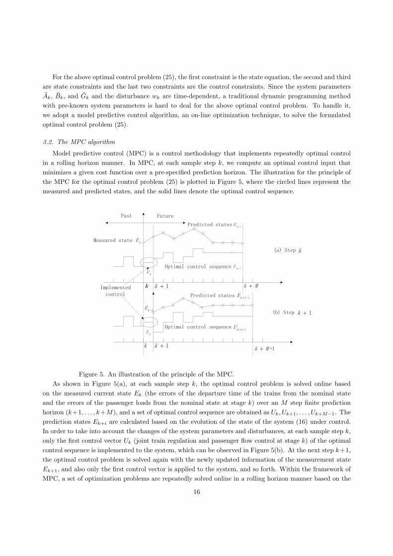
Model predictive control (MPC) is a control methodology that implements repeatedly optimal control

in a rolling horizon manner. In MPC, at each sample step k, we compute an optimal control input that

minimizes a given cost function over a pre-specified prediction horizon. The illustration for the principle of

the MPC for the optimal control problem (25) is plotted in Figure 5, where the circled lines represent the

measured and predicted states, and the solid lines denote the optimal control sequence.

Figure 5. An illustration of the principle of the MPC.

As shown in Figure 5(a), at each sample step k, the optimal control problem is solved online based

on the measured current state Ek (the errors of the departure time of the trains from the nominal state

and the errors of the passenger loads from the nominal state at stage k) over an M step finite prediction

horizon (k+1, . . . , k+M), and a set of optimal control sequence are obtained as Uk, Uk+1, . . . , Uk+M−1. The

prediction states Ek+i are calculated based on the evolution of the state of the system (16) under control.

In order to take into account the changes of the system parameters and disturbances, at each sample step k,

only the first control vector Uk (joint train regulation and passenger flow control at stage k) of the optimal

control sequence is implemented to the system, which can be observed in Figure 5(b). At the next step k+1,

the optimal control problem is solved again with the newly updated information of the measurement state

Ek+1, and also only the first control vector is applied to the system, and so forth. Within the framework of

MPC, a set of optimization problems are repeatedly solved online in a rolling horizon manner based on the

16

real-time updated system information, which makes this method efficient to solve the above optimal control

problem (25) with the updated system parameters and disturbances.

Specifically, the MPC approach for the metro lines can be characterized by the following three compo-

nents:

(1) The prediction model of system.

The prediction model of the dynamic system is used to predict the effects of the control inputs on the

evolution of the dynamic system over a given prediction horizon and to determine the control strategy that

optimizes a given cost function. For the metro line system, the proposed model (16) of the metro line system

is used to predict the future errors of the departure time of the trains and the future errors of the passenger

loads of the trains based on the measured current state Ek.

(2) The optimization problem.

Based on the model of the dynamic system, at each sample step k, the optimization problem over a

given prediction horizon is solved online, which determines a set of optimal control sequences. For the metro

line system, the optimization determines the joint train regulation and passenger flow control strategy that

improves the headway regularity and commercial speed of high-frequency metro lines under the constraints

based on the updated information of the measurements. Specially, at each sample step k, associated with

(25) is the following optimization problem to compute the control input.

minUk+j

M−1∑j=0

{ET

k+j+1PEk+j+1 + (Ek+j+1 − Ek+j)TQ(Ek+j+1 − Ek+j) + UT

k+jRUk+j

}(26)

s.t. Ek+j+1 = Ak+jEk+j + Bk+jUk+j + Gk+jwk+j ,

H1(Ek+j − Ek+j+1) ≤ (H − tmin)IN×1,

H2Ek+j+1 ≤ Lk+j+1,

Uk+j ≤ Umax,

− Uk+j ≤ −Umin, j = 0, 1, . . . ,M − 1.

(3) The rolling horizon.

When the optimal control input is obtained from the optimization, the first control vector of the optimal

result is implemented to the process. At the next step k + 1, the prediction model (16) of the metro line

system receives the new measured information, the whole prediction horizon is shifted one step forward, and

the optimization starts again. This rolling horizon scheme makes MPC a closed-loop control, which enables

the system to get feedback from real time information.

Moreover, at each sample step k, the above optimization problem (26) can be converted to a quadratic

programming (QP) problem. Define E = [ETk+1, E

Tk+2, . . . , E

Tk+M ]T and U = [UT

k , UTk+1, . . . , U

Tk+M−1]

T .

Then at each prediction step k, for the measured current state Ek, the state prediction for the M step finite

horizon problem is obtained from the state equation of (26) as follows.

E = FEk +ΦU, (27)

where the definitions of matrices F and Φ are given in Appendix C.

Thus the optimal joint train regulation and passenger flow control strategy is reduced to the problem of

solving a set of quadratic programming (QP) problems at different steps. According to equation (27), the

equivalent QP formulation at step k for the optimization problem (26) is presented as follows.

minU

J = UT (ΦT PΦ+ ΦT QΦ+ R)U + 2UT (ΦT PFEk +ΦT QFEk) + Ψ (28)

17

s.t.

H3H4Φ

H6Φ

I2MN

−I2MN

U ≤

(H − tmin)IMN×1 −H3H4FEk −H3H5Ek

L−H6FEk

Umax

−Umin

,

where Ψ = FT PFE2k +FT QFE2

k is a constant, the weighted matrixes P , Q and R can be directly obtained

from the cost function of (26), L = [LTk+1, L

Tk+2, . . . , L

Tk+M ]T , Umax = [UT

max, UTmax, . . . , U

Tmax]

T2MN×1, Umin =

[UTmin, U

Tmin, . . . , U

Tmin]

T2MN×1. The derivation of (28) from (26) is given in Appendix D. The other matrices

H3, H4, H5, H6 are defined in Appendix D.

According to the formulated quadratic programming (QP) problem, the main algorithm of the joint

optimal train regulation and passenger flow control strategy for metro lines under disturbances is summarized

as follows.

Algorithm 3.1.

• Step 1. At each sample step k, obtain the measured state Ek for the error joint dynamic model (16)

with the undated parameters and disturbances.

• Step 2. According to the measured state Ek, for the given prediction horizon M , calculate the system

parameters F and Φ for the error joint dynamic model (16) based on the formulation (27).

• Step 3. For the measured state Ek and obtained system parameters F and Φ, formulate the quadratic

programming (QP) problem (28).

• Step 4. By solving the quadratic programming(QP) problem (28), get the joint optimal train regulation

and passenger flow control strategy U and apply it to the joint dynamic model (16) to obtain the next

value Ek+1.

• Step 5. Based on the measured value Ek+1, repeat Steps 1-4 until the step horizon jf .

It should be noted that the measured current state Ek includes the current errors of the departure time

of train from the nominal state (tij − T ij ) and the current errors of the passenger loads from the nominal

state (lij − Lij). At each decision step, the actual departure time of trains can be easily obtained by the

metro regulation department. In particular, with the highly developed monitoring equipments applied in

each carriage of the train, the actual passenger load of trains at each decision step can be measured more

accurately. The actual passenger loads of each train are also available during the algorithm execution. Thus,

the system states (departure time and passenger load) of metro lines are fully observable. In addition, at

each step k, based on the measured current state Ek, we need to predict the near-future states (departure

time and passenger load) of trains over an M step finite prediction horizon (k + 1, . . . , k + M) during a

short time period, where the states of the trains at stage k +M is the “boundary” which is not controlled.

Within the framework of MPC, we use a dynamic evolution model (16) to predict the near-future states

of the trains based on the measured current state Ek. For the system parameters of (16), we assume that

the passenger arrival rate γij does not change during a short time period of the prediction horizon, which is

chosen from the measured value at step k. The disembarking proportionality factor βij during the prediction

horizon is chosen from the estimated values by using the historical data.

According to the proposed MPC algorithm, the optimal control problem (25) for the joint optimal

train regulation and passenger flow control strategy is formulated as a set of quadratic programming(QP)

18

problems. By choosing the proper prediction step, the proposed MPC algorithm can reduce the number of

variables and constraints for the formulated quadratic programming(QP) problems, which leads to a low

online computational burden of the MPC algorithm. Thus the proposed MPC algorithm is effective in

dealing with the large-scale nonlinear optimization problem for metro lines.

3.3. Stability analysis

In practice, due to the instability of many metro line systems, it is desirable to design a train regulation

algorithm to ensure stability of the metro line. To further reveal the feature of the proposed MPC algo-

rithm for the joint optimal train regulation and passenger flow control strategy, we analyze the stability

(convergence) of the metro line system under the proposed MPC algorithm.

The stability of the metro line system under the MPC algorithm is a complex function of the MPC

parameters P , Q, R, Ak, Bk, Lk, Umax and Umin. Consider the state and control constraints for the metro

line system with the overcrowded passenger arrival flow. It becomes more difficult to analyze the system

stability. In particular, MPC has the advantage to cope with hard constraints on states and controls of

the system. MPC of constrained systems is nonlinear necessitating the use of Lyapunov stability theory for

system stability analysis. The value function of the optimization problem could be employed as a Lyapunov

function for establishing stability of the model predictive control of the constrained discrete-time system

(Mayne et al., 2000). Correspondingly, for the proposed MPC algorithm in this study, one can also apply

the value function of the optimization problem (25) as a Lyapunov function to analyze the stability of the

metro line system with state and control constraints.

To discuss the stability of the metro line system, we consider the joint error dynamic model (16) without

disturbances wj , i.e., wj = 0. Then based on Lyapunov stability theory, we present the stability result of

the joint error dynamic model under the proposed MPC algorithm as the following theorem.

Theorem 3.1. Consider the joint error dynamic model (16) under the proposed MPC algorithm based on

the following optimization problem

minU

J(U,Ek) =

M−1∑j=0

{ET

k+j+1PEk+j+1 + (Ek+j+1 − Ek+j)TQ(Ek+j+1 − Ek+j) + UT

k+jRUk+j

}(29)

s.t. Ek+j+1 = Ak+jEk+j + Bk+jUk+j + Gk+jwk+j ,

H1(Ek+j − Ek+j+1) ≤ (H − tmin)IN×1,

H2Ek+j+1 ≤ Lk+j+1,

Uk+j ≤ Umax,

− Uk+j ≤ −Umin, j = 0, 1, . . . ,M − 1.

Suppose that the above optimization problem is feasible at the initial time k = j0, the system parameters Ak

and Bk are given, and Ek+M = 0. Then for all P > 0, Q > 0, and R > 0, it holds that limk→∞ Ek = 0,

that is, the joint error dynamic model (16) under the proposed MPC algorithm is stable at zero subject to

the constraints, and the actual timetable converges to the nominal timetable.

Proof. At first, for the joint error dynamic model (16) under the proposed MPC algorithm, we choose the

value function of the above optimization problem (29) as a Lyapunov function, i.e.,

V (k) = J(U∗(k), Ek), (30)

19

where U∗(k) = {U∗k , U

∗k+1, . . . , U

∗k+M−1} denotes the optimal control sequence for the optimal problem (29).

It is clear that V (k) is non-negative.

Then for the optimal control solutions U∗(k) at step k, we can further get the state vector E(k) =

[ETk+1, E

Tk+2, . . . , E

Tk+M ]T at step k. It is clear that U∗(k) and E(k) satisfy the constraints. Thus for the

next step k+1, we construct the control sequence U(k+1) = {U∗k+1, U

∗k+2, . . . , U

∗k+M−1, 0}. It is clear that

U(k + 1) is feasible at step k + 1 for the optimal problem (29). By substituting U(k + 1) into the objective

function, we can obtain J(U(k + 1), Ek+1). Then by combining the assumption Ek+M = 0, we have

V (k + 1) = J(U∗(k + 1), Ek+1)

≤ J(U(k + 1), Ek+1)

= V (k)− ETk+1PEk+1 − (Ek+1 − Ek)

TQ(Ek+1 − Ek)− UTk RUk, (31)

which means that V (k+1)− V (k) ≤ 0, and V (k) is decreasing and lower-bounded by 0. Then according to

Lyapunov stability theory, it holds that limk→∞ Ek = 0, i.e., the joint error dynamic model (16) under the

proposed MPC algorithm is stable at zero subject to the constraints, and the actual timetable will converge

to the nominal timetable. The proof is complete.

The result in Theorem 3.1 indicates the proposed MPC algorithm ensures the stability of the joint train

traffic system without disturbances, which means that when the disturbances for the train regulation system

disappear, the train traffic system converges to a stable state, which guarantees a good performance for the

train regulation system. With the assumption of the observability, the considered metro line system is

stable under the proposed MPC algorithm, which also reveals the controllability of the considered metro

line system. Moreover, it should be noted that since the proposed MPC algorithm is based on state-

feedback information, which allows the train to effectively adjust its speed as time evolves, and thus it is

robust to uncertainty and disturbances. In addition, the considered objective function in this study takes a

positive definite quadratic form. Thus the corresponding value function is also positive definite, which can

be adopted as a Lyapunov function. If we change the control criteria to minimize the maximum span, the

corresponding objective function of the formulated optimization problem will be changed, which may not

be a positive definite quadratic form. Under this case, the value function of the optimization problem may

not be employed as a Lyapunov function for establishing a stability condition. The stability analysis will

become more difficult, which may resort to other methods for stability analysis.

4. Numerical Examples

In this section, to demonstrate the performance of the proposed joint optimal dynamic train regulation

and passenger flow control strategy for metro lines, we apply our proposed model and method to the actual

Beijing metro line 9 that consists of 13 stations (i.e., N = 12) through three traffic scenarios. Beijing metro

line 9 is a busy metro line including the largest railway station of Beijing (Beijing West Railway) and six

transfer stations. During the peak hours of the day, the passenger flow in many stations is extremely large,

which makes the arriving train usually overloaded and largely affects the operational efficiency and also

leads to a safety hazard for the metro line system. Thus, it is necessary to design a joint dynamic train

regulation and passenger flow control strategy to manage the entire metro line system, for improving the

headway regularity and commercial speed under uncertain disturbances.

20

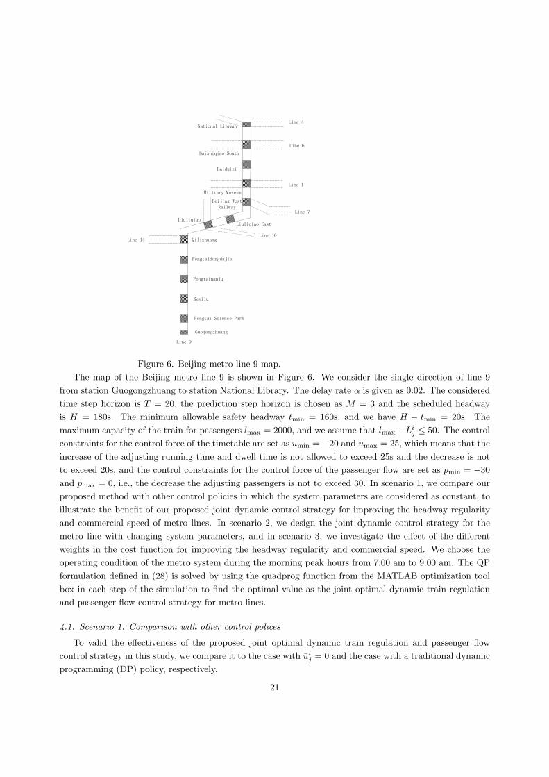
Figure 6. Beijing metro line 9 map.

The map of the Beijing metro line 9 is shown in Figure 6. We consider the single direction of line 9

from station Guogongzhuang to station National Library. The delay rate α is given as 0.02. The considered

time step horizon is T = 20, the prediction step horizon is chosen as M = 3 and the scheduled headway

is H = 180s. The minimum allowable safety headway tmin = 160s, and we have H − tmin = 20s. The

maximum capacity of the train for passengers lmax = 2000, and we assume that lmax−Lij ≤ 50. The control

constraints for the control force of the timetable are set as umin = −20 and umax = 25, which means that the

increase of the adjusting running time and dwell time is not allowed to exceed 25s and the decrease is not

to exceed 20s, and the control constraints for the control force of the passenger flow are set as pmin = −30

and pmax = 0, i.e., the decrease the adjusting passengers is not to exceed 30. In scenario 1, we compare our

proposed method with other control policies in which the system parameters are considered as constant, to

illustrate the benefit of our proposed joint dynamic control strategy for improving the headway regularity

and commercial speed of metro lines. In scenario 2, we design the joint dynamic control strategy for the

metro line with changing system parameters, and in scenario 3, we investigate the effect of the different

weights in the cost function for improving the headway regularity and commercial speed. We choose the

operating condition of the metro system during the morning peak hours from 7:00 am to 9:00 am. The QP

formulation defined in (28) is solved by using the quadprog function from the MATLAB optimization tool

box in each step of the simulation to find the optimal value as the joint optimal dynamic train regulation

and passenger flow control strategy for metro lines.

4.1. Scenario 1: Comparison with other control polices

To valid the effectiveness of the proposed joint optimal dynamic train regulation and passenger flow

control strategy in this study, we compare it to the case with uij = 0 and the case with a traditional dynamic

programming (DP) policy, respectively.

21

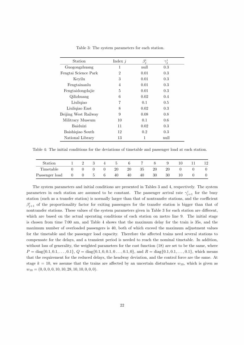
Table 3: The system parameters for each station.

Station Index j βij γi

j

Guogongzhuang 1 null 0.3

Fengtai Science Park 2 0.01 0.3

Keyilu 3 0.01 0.3

Fengtainanlu 4 0.01 0.3

Fengtaidongdajie 5 0.01 0.3

Qilizhuang 6 0.02 0.4

Liuliqiao 7 0.1 0.5

Liuliqiao East 8 0.02 0.3

Beijing West Railway 9 0.08 0.8

Militrary Museum 10 0.1 0.6

Baiduizi 11 0.02 0.3

Baishiqiao South 12 0.2 0.3

National Library 13 1 null

Table 4: The initial conditions for the deviations of timetable and passenger load at each station.

Station 1 2 3 4 5 6 7 8 9 10 11 12

Timetable 0 0 0 0 20 20 35 20 20 0 0 0

Passenger load 0 0 5 6 40 40 40 30 30 10 0 0

The system parameters and initial conditions are presented in Tables 3 and 4, respectively. The system

parameters in each station are assumed to be constant. The passenger arrival rate γij+1 for the busy

station (such as a transfer station) is normally larger than that of nontransfer stations, and the coefficient

βij+1 of the proportionality factor for exiting passengers for the transfer station is bigger than that of

nontransfer stations. These values of the system parameters given in Table 3 for each station are different,

which are based on the actual operating conditions of each station on metro line 9. The initial stage

is chosen from time 7:00 am, and Table 4 shows that the maximum delay for the train is 35s, and the

maximum number of overloaded passengers is 40, both of which exceed the maximum adjustment values

for the timetable and the passenger load capacity. Therefore the affected trains need several stations to

compensate for the delays, and a transient period is needed to reach the nominal timetable. In addition,

without loss of generality, the weighted parameters for the cost function (18) are set to be the same, where

P = diag{0.1, 0.1, . . . , 0.1}, Q = diag{0.1, 0, 0.1, 0 . . . , 0.1, 0}, and R = diag{0.1, 0.1, . . . , 0.1}, which means

that the requirement for the reduced delays, the headway deviation, and the control force are the same. At

stage k = 10, we assume that the trains are affected by an uncertain disturbance w10, which is given as

w10 = (0, 0, 0, 0, 10, 10, 28, 10, 10, 0, 0, 0).

22

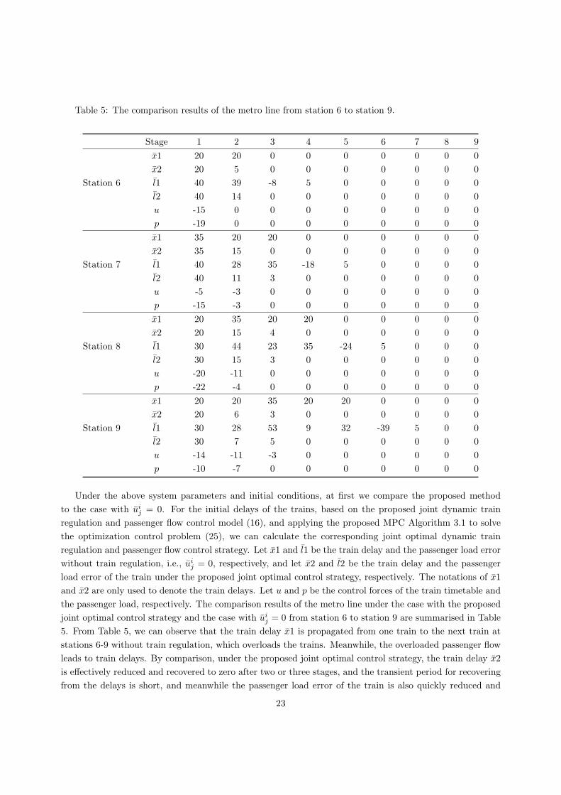
Table 5: The comparison results of the metro line from station 6 to station 9.

Stage 1 2 3 4 5 6 7 8 9

x1 20 20 0 0 0 0 0 0 0

x2 20 5 0 0 0 0 0 0 0

Station 6 l1 40 39 -8 5 0 0 0 0 0

l2 40 14 0 0 0 0 0 0 0

u -15 0 0 0 0 0 0 0 0

p -19 0 0 0 0 0 0 0 0

x1 35 20 20 0 0 0 0 0 0

x2 35 15 0 0 0 0 0 0 0

Station 7 l1 40 28 35 -18 5 0 0 0 0

l2 40 11 3 0 0 0 0 0 0

u -5 -3 0 0 0 0 0 0 0

p -15 -3 0 0 0 0 0 0 0

x1 20 35 20 20 0 0 0 0 0

x2 20 15 4 0 0 0 0 0 0

Station 8 l1 30 44 23 35 -24 5 0 0 0

l2 30 15 3 0 0 0 0 0 0

u -20 -11 0 0 0 0 0 0 0

p -22 -4 0 0 0 0 0 0 0

x1 20 20 35 20 20 0 0 0 0

x2 20 6 3 0 0 0 0 0 0

Station 9 l1 30 28 53 9 32 -39 5 0 0

l2 30 7 5 0 0 0 0 0 0

u -14 -11 -3 0 0 0 0 0 0

p -10 -7 0 0 0 0 0 0 0

Under the above system parameters and initial conditions, at first we compare the proposed method

to the case with uij = 0. For the initial delays of the trains, based on the proposed joint dynamic train

regulation and passenger flow control model (16), and applying the proposed MPC Algorithm 3.1 to solve

the optimization control problem (25), we can calculate the corresponding joint optimal dynamic train

regulation and passenger flow control strategy. Let x1 and l1 be the train delay and the passenger load error

without train regulation, i.e., uij = 0, respectively, and let x2 and l2 be the train delay and the passenger

load error of the train under the proposed joint optimal control strategy, respectively. The notations of x1

and x2 are only used to denote the train delays. Let u and p be the control forces of the train timetable and

the passenger load, respectively. The comparison results of the metro line under the case with the proposed

joint optimal control strategy and the case with uij = 0 from station 6 to station 9 are summarised in Table

5. From Table 5, we can observe that the train delay x1 is propagated from one train to the next train at

stations 6-9 without train regulation, which overloads the trains. Meanwhile, the overloaded passenger flow

leads to train delays. By comparison, under the proposed joint optimal control strategy, the train delay x2

is effectively reduced and recovered to zero after two or three stages, and the transient period for recovering

from the delays is short, and meanwhile the passenger load error of the train is also quickly reduced and

23

converges to the nominal level after three stages. In addition, from Table 5, we can find that under uij = 0,

the train delay x1 lasts for about three to five stages for stations 6-9 and the corresponding values of the

train delays are from 20s to 35s, while the control force u for the train timetable only needs two stages for

recovering from the delays at stations 6-9 and the values of the control force u are less than the train delay

value x1, which shows that the joint optimal control strategy improves the efficiency for the metro lines

recovering from disturbed situations.

1 2 3 4 5 6 7 8 9 10 11 12 13 14 15 16 17 18 19 20−10

0

10

20

30

Stage k

Tra

indel

ay

ti j−

Ti j

1 2 3 4 5 6 7 8 9 10 11 12 13 14 15 16 17 18 19 20

−20

0

20

40

Stage k

Load

erro

rli j−

Li j

station 6station 7station 8station 9

(a)

(b)

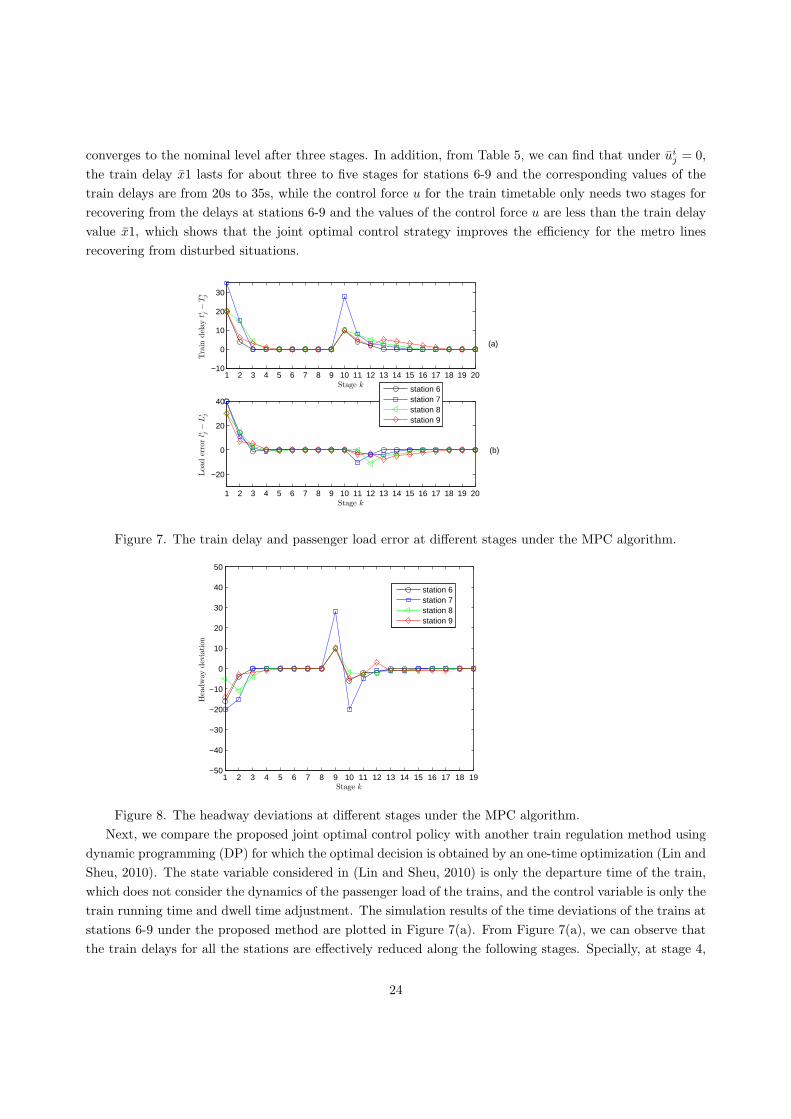
Figure 7. The train delay and passenger load error at different stages under the MPC algorithm.

1 2 3 4 5 6 7 8 9 10 11 12 13 14 15 16 17 18 19−50

−40

−30

−20

−10

0

10

20

30

40

50

Stage k

Hea

dw

ay

dev

iation

station 6station 7station 8station 9

Figure 8. The headway deviations at different stages under the MPC algorithm.

Next, we compare the proposed joint optimal control policy with another train regulation method using

dynamic programming (DP) for which the optimal decision is obtained by an one-time optimization (Lin and

Sheu, 2010). The state variable considered in (Lin and Sheu, 2010) is only the departure time of the train,

which does not consider the dynamics of the passenger load of the trains, and the control variable is only the

train running time and dwell time adjustment. The simulation results of the time deviations of the trains at

stations 6-9 under the proposed method are plotted in Figure 7(a). From Figure 7(a), we can observe that

the train delays for all the stations are effectively reduced along the following stages. Specially, at stage 4,

24

the train delays are reduced to zero and the trains are operating according to the nominal timetable, and the

full timetable recovery is achieved, which indicates the stability of the metro line system under the proposed

method. Moreover, at stage 10, when the trains are affected by the uncertain disturbance that further leads

to delays of the trains, the joint optimal control strategy can be calculated in real-time according to the

current disturbance, and under the new joint optimal control strategy, the delays of the trains are reduced

along the stages, and are all stabilized to zero after a few stages. In addition, the errors of passenger load

at the different stages under the joint optimal control strategy are plotted in Figure 7(b), which shows that

the errors of passenger load are reduced along the stages and kept at zero at stage 4, which ensures that

the passenger load of the trains are kept at a reasonable level. Additionally, the headway deviations for

the trains under the joint optimal control at stations 6-9 are plotted in Figure 8, which shows that when

the disturbance happens, there are fluctuations for the headway deviations from the nominal headway, and

then the headway deviations converge to zero, i.e., the actual headway is kept at the nominal state and the

headway regularity is improved. The headway regularity of the metro line reduces the average waiting time

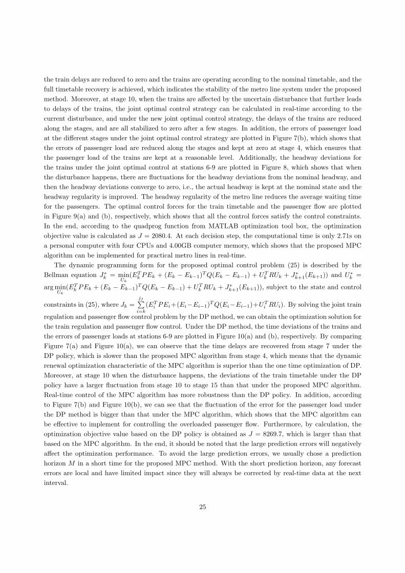
for the passengers. The optimal control forces for the train timetable and the passenger flow are plotted

in Figure 9(a) and (b), respectively, which shows that all the control forces satisfy the control constraints.

In the end, according to the quadprog function from MATLAB optimization tool box, the optimization

objective value is calculated as J = 2080.4. At each decision step, the computational time is only 2.71s on

a personal computer with four CPUs and 4.00GB computer memory, which shows that the proposed MPC

algorithm can be implemented for practical metro lines in real-time.

The dynamic programming form for the proposed optimal control problem (25) is described by the

Bellman equation J∗k = min

Uk

(ETk PEk + (Ek − Ek−1)

TQ(Ek − Ek−1) + UTk RUk + J∗

k+1(Ek+1)) and U∗k =

argminUk

(ETk PEk + (Ek − Ek−1)

TQ(Ek − Ek−1) + UTk RUk + J∗

k+1(Ek+1)), subject to the state and control

constraints in (25), where Jk =jf∑i=k

(ETi PEi+(Ei−Ei−1)

TQ(Ei−Ei−1)+UTi RUi). By solving the joint train

regulation and passenger flow control problem by the DP method, we can obtain the optimization solution for

the train regulation and passenger flow control. Under the DP method, the time deviations of the trains and

the errors of passenger loads at stations 6-9 are plotted in Figure 10(a) and (b), respectively. By comparing

Figure 7(a) and Figure 10(a), we can observe that the time delays are recovered from stage 7 under the

DP policy, which is slower than the proposed MPC algorithm from stage 4, which means that the dynamic

renewal optimization characteristic of the MPC algorithm is superior than the one time optimization of DP.

Moreover, at stage 10 when the disturbance happens, the deviations of the train timetable under the DP

policy have a larger fluctuation from stage 10 to stage 15 than that under the proposed MPC algorithm.

Real-time control of the MPC algorithm has more robustness than the DP policy. In addition, according

to Figure 7(b) and Figure 10(b), we can see that the fluctuation of the error for the passenger load under

the DP method is bigger than that under the MPC algorithm, which shows that the MPC algorithm can

be effective to implement for controlling the overloaded passenger flow. Furthermore, by calculation, the

optimization objective value based on the DP policy is obtained as J = 8269.7, which is larger than that

based on the MPC algorithm. In the end, it should be noted that the large prediction errors will negatively

affect the optimization performance. To avoid the large prediction errors, we usually chose a prediction

horizon M in a short time for the proposed MPC method. With the short prediction horizon, any forecast

errors are local and have limited impact since they will always be corrected by real-time data at the next

interval.

25

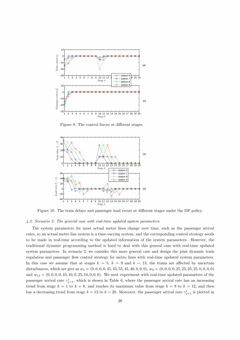
1 2 3 4 5 6 7 8 9 10 11 12 13 14 15 16 17 18 19 20−30

−20

−10

0

10

Stage k

Tra

inco

ntr

olu

i j

1 2 3 4 5 6 7 8 9 10 11 12 13 14 15 16 17 18 19 20−30

−20

−10

0

10

Stage k

Pass

enger

contr

olp

I j

station 6station 7station 8station 9

(a)

(b)

Figure 9. The control forces at different stages.

1 2 3 4 5 6 7 8 9 10 11 12 13 14 15 16 17 18 19 200

10

20

30

40

Stage k

Tra

indel

ay

ti j−

Ti j

1 2 3 4 5 6 7 8 9 10 11 12 13 14 15 16 17 18 19 20−40

−20

0

20

40

60

Stage k

Load

erro

rli j−

Li j

station 6station 7station 8station 9

(a)

(b)

Figure 10. The train delays and passenger load errors at different stages under the DP policy.

4.2. Scenario 2: The general case with real-time updated system parameters

The system parameters for most actual metro lines change over time, such as the passenger arrival

rates, so an actual metro line system is a time-varying system, and the corresponding control strategy needs

to be made in real-time according to the updated information of the system parameters. However, the

traditional dynamic programming method is hard to deal with this general case with real-time updated

system parameters. In scenario 2, we consider this more general case and design the joint dynamic train

regulation and passenger flow control strategy for metro lines with real-time updated system parameters.

In this case we assume that at stages k = 5, k = 9 and k = 13, the trains are affected by uncertain

disturbances, which are give as w5 = (0, 0, 0, 0, 45, 45, 55, 45, 40, 0, 0, 0), w9 = (0, 0, 0, 0, 25, 25, 25, 25, 0, 0, 0, 0)

and w13 = (0, 0, 0, 0, 10, 10, 0, 25, 10, 0, 0, 0). We next experiment with real-time updated parameters of the

passenger arrival rate γij+1, which is shown in Table 6, where the passenger arrival rate has an increasing

trend from stage k = 1 to k = 8, and reaches its maximum value from stage k = 9 to k = 12, and then

has a decreasing trend from stage k = 13 to k = 20. Moreover, the passenger arrival rate γij+1 is plotted in

26

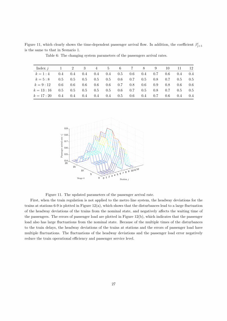
Figure 11, which clearly shows the time-dependent passenger arrival flow. In addition, the coefficient βij+1

is the same to that in Scenario 1.

Table 6: The changing system parameters of the passengers arrival rates.

Index j 1 2 3 4 5 6 7 8 9 10 11 12

k = 1 : 4 0.4 0.4 0.4 0.4 0.4 0.5 0.6 0.4 0.7 0.6 0.4 0.4

k = 5 : 8 0.5 0.5 0.5 0.5 0.5 0.6 0.7 0.5 0.8 0.7 0.5 0.5

k = 9 : 12 0.6 0.6 0.6 0.6 0.6 0.7 0.8 0.6 0.9 0.8 0.6 0.6

k = 13 : 16 0.5 0.5 0.5 0.5 0.5 0.6 0.7 0.5 0.8 0.7 0.5 0.5

k = 17 : 20 0.4 0.4 0.4 0.4 0.4 0.5 0.6 0.4 0.7 0.6 0.4 0.4

0 1 2 3 4 5 6 7 8 9 101112

0

5

10

15

200.4

0.5

0.6

0.7

0.8

0.9

Station jStage k

Pass

enger

arr

ivalra

teγ

i j

Figure 11. The updated parameters of the passenger arrival rate.

First, when the train regulation is not applied to the metro line system, the headway deviations for the

trains at stations 6-9 is plotted in Figure 12(a), which shows that the disturbances lead to a large fluctuation

of the headway deviations of the trains from the nominal state, and negatively affects the waiting time of

the passengers. The errors of passenger load are plotted in Figure 12(b), which indicates that the passenger

load also has large fluctuations from the nominal state. Because of the multiple times of the disturbances

to the train delays, the headway deviations of the trains at stations and the errors of passenger load have

multiple fluctuations. The fluctuations of the headway deviations and the passenger load error negatively

reduce the train operational efficiency and passenger service level.

27

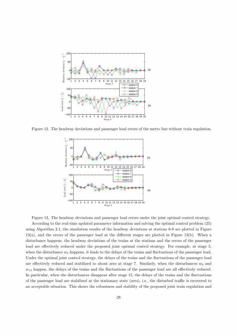
1 2 3 4 5 6 7 8 9 10 11 12 13 14 15 16 17 18 19−50

0

50

100

Stage k

Hea

dw

ay

dev

iation

ti j−

ti−

1

j

1 2 3 4 5 6 7 8 9 10 11 12 13 14 15 16 17 18 19 20−100

−50

0

50

100

Load

erro

rli j−

Li j

Stage k

station 6station 7station 8station 9

(a)

(b)

Figure 12. The headway deviations and passenger load errors of the metro line without train regulation.

1 2 3 4 5 6 7 8 9 10 11 12 13 14 15 16 17 18 19−50

0

50

100

Stage k

Hea

dw

ay

dev

iation

ti j−

ti−

1

j

1 2 3 4 5 6 7 8 9 10 11 12 13 14 15 16 17 18 19 20−100

−50

0

50

100

Stage k

Load

erro

rli j−

Li j

station 6station 7station 8station 9

(a)

(b)

Figure 13. The headway deviations and passenger load errors under the joint optimal control strategy.

According to the real-time updated parameter information and solving the optimal control problem (25)

using Algorithm 3.1, the simulation results of the headway deviations at stations 6-9 are plotted in Figure

13(a), and the errors of the passenger load at the different stages are plotted in Figure 13(b). When a

disturbance happens, the headway deviations of the trains at the stations and the errors of the passenger

load are effectively reduced under the proposed joint optimal control strategy. For example, at stage 5,

when the disturbance w5 happens, it leads to the delays of the trains and fluctuations of the passenger load.

Under the optimal joint control strategy, the delays of the trains and the fluctuations of the passenger load

are effectively reduced and stabilized to about zero at stage 7. Similarly, when the disturbances w9 and

w13 happen, the delays of the trains and the fluctuations of the passenger load are all effectively reduced.

In particular, when the disturbances disappear after stage 15, the delays of the trains and the fluctuations

of the passenger load are stabilized at the stationary state (zero), i.e., the disturbed traffic is recovered to

an acceptable situation. This shows the robustness and stability of the proposed joint train regulation and

28

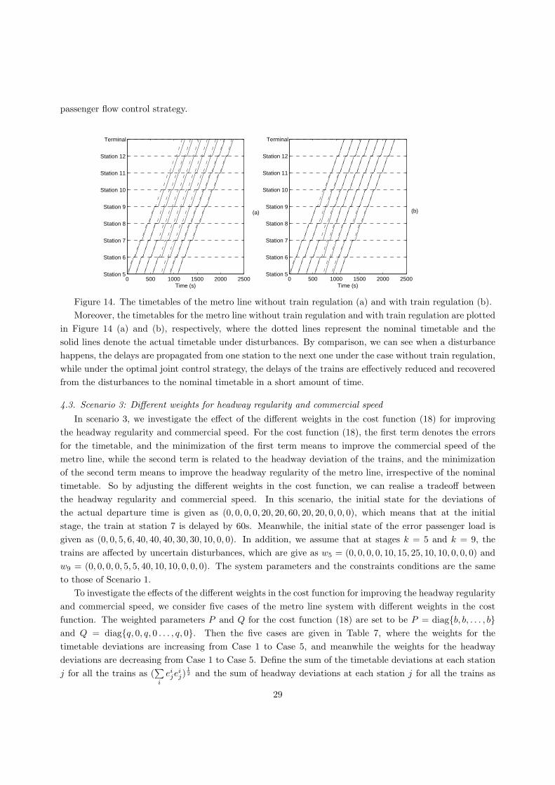
passenger flow control strategy.

0 500 1000 1500 2000 2500Station 5

Station 6

Station 7

Station 8

Station 9

Station 10

Station 11

Station 12

Terminal

Time (s)0 500 1000 1500 2000 2500

Station 5

Station 6

Station 7

Station 8

Station 9

Station 10

Station 11

Station 12

Terminal

Time (s)

(b)(a)

Figure 14. The timetables of the metro line without train regulation (a) and with train regulation (b).

Moreover, the timetables for the metro line without train regulation and with train regulation are plotted

in Figure 14 (a) and (b), respectively, where the dotted lines represent the nominal timetable and the

solid lines denote the actual timetable under disturbances. By comparison, we can see when a disturbance

happens, the delays are propagated from one station to the next one under the case without train regulation,

while under the optimal joint control strategy, the delays of the trains are effectively reduced and recovered

from the disturbances to the nominal timetable in a short amount of time.

4.3. Scenario 3: Different weights for headway regularity and commercial speed

In scenario 3, we investigate the effect of the different weights in the cost function (18) for improving

the headway regularity and commercial speed. For the cost function (18), the first term denotes the errors

for the timetable, and the minimization of the first term means to improve the commercial speed of the

metro line, while the second term is related to the headway deviation of the trains, and the minimization

of the second term means to improve the headway regularity of the metro line, irrespective of the nominal

timetable. So by adjusting the different weights in the cost function, we can realise a tradeoff between

the headway regularity and commercial speed. In this scenario, the initial state for the deviations of

the actual departure time is given as (0, 0, 0, 0, 20, 20, 60, 20, 20, 0, 0, 0), which means that at the initial

stage, the train at station 7 is delayed by 60s. Meanwhile, the initial state of the error passenger load is

given as (0, 0, 5, 6, 40, 40, 40, 30, 30, 10, 0, 0). In addition, we assume that at stages k = 5 and k = 9, the

trains are affected by uncertain disturbances, which are give as w5 = (0, 0, 0, 0, 10, 15, 25, 10, 10, 0, 0, 0) and

w9 = (0, 0, 0, 0, 5, 5, 40, 10, 10, 0, 0, 0). The system parameters and the constraints conditions are the same

to those of Scenario 1.

To investigate the effects of the different weights in the cost function for improving the headway regularity

and commercial speed, we consider five cases of the metro line system with different weights in the cost

function. The weighted parameters P and Q for the cost function (18) are set to be P = diag{b, b, . . . , b}and Q = diag{q, 0, q, 0 . . . , q, 0}. Then the five cases are given in Table 7, where the weights for the

timetable deviations are increasing from Case 1 to Case 5, and meanwhile the weights for the headway

deviations are decreasing from Case 1 to Case 5. Define the sum of the timetable deviations at each station

j for all the trains as (∑i

eijeij)

12 and the sum of headway deviations at each station j for all the trains as

29

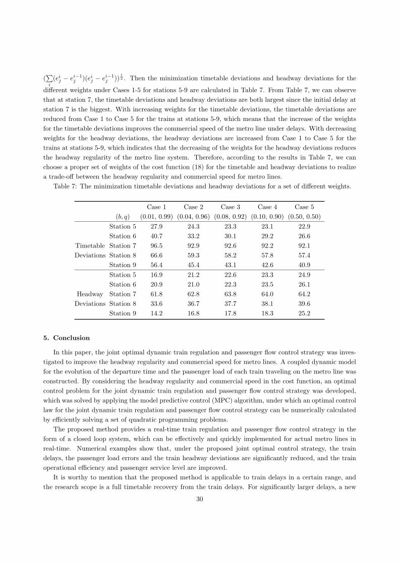
(∑i

(eij − ei−1j )(eij − ei−1

j ))12 . Then the minimization timetable deviations and headway deviations for the

different weights under Cases 1-5 for stations 5-9 are calculated in Table 7. From Table 7, we can observe

that at station 7, the timetable deviations and headway deviations are both largest since the initial delay at

station 7 is the biggest. With increasing weights for the timetable deviations, the timetable deviations are

reduced from Case 1 to Case 5 for the trains at stations 5-9, which means that the increase of the weights

for the timetable deviations improves the commercial speed of the metro line under delays. With decreasing

weights for the headway deviations, the headway deviations are increased from Case 1 to Case 5 for the

trains at stations 5-9, which indicates that the decreasing of the weights for the headway deviations reduces

the headway regularity of the metro line system. Therefore, according to the results in Table 7, we can

choose a proper set of weights of the cost function (18) for the timetable and headway deviations to realize

a trade-off between the headway regularity and commercial speed for metro lines.

Table 7: The minimization timetable deviations and headway deviations for a set of different weights.

Case 1 Case 2 Case 3 Case 4 Case 5

(b, q) (0.01, 0.99) (0.04, 0.96) (0.08, 0.92) (0.10, 0.90) (0.50, 0.50)

Station 5 27.9 24.3 23.3 23.1 22.9

Station 6 40.7 33.2 30.1 29.2 26.6

Timetable Station 7 96.5 92.9 92.6 92.2 92.1

Deviations Station 8 66.6 59.3 58.2 57.8 57.4

Station 9 56.4 45.4 43.1 42.6 40.9

Station 5 16.9 21.2 22.6 23.3 24.9

Station 6 20.9 21.0 22.3 23.5 26.1

Headway Station 7 61.8 62.8 63.8 64.0 64.2

Deviations Station 8 33.6 36.7 37.7 38.1 39.6

Station 9 14.2 16.8 17.8 18.3 25.2

5. Conclusion

In this paper, the joint optimal dynamic train regulation and passenger flow control strategy was inves-

tigated to improve the headway regularity and commercial speed for metro lines. A coupled dynamic model

for the evolution of the departure time and the passenger load of each train traveling on the metro line was

constructed. By considering the headway regularity and commercial speed in the cost function, an optimal

control problem for the joint dynamic train regulation and passenger flow control strategy was developed,

which was solved by applying the model predictive control (MPC) algorithm, under which an optimal control

law for the joint dynamic train regulation and passenger flow control strategy can be numerically calculated

by efficiently solving a set of quadratic programming problems.

The proposed method provides a real-time train regulation and passenger flow control strategy in the

form of a closed loop system, which can be effectively and quickly implemented for actual metro lines in

real-time. Numerical examples show that, under the proposed joint optimal control strategy, the train

delays, the passenger load errors and the train headway deviations are significantly reduced, and the train

operational efficiency and passenger service level are improved.

It is worthy to mention that the proposed method is applicable to train delays in a certain range, and

the research scope is a full timetable recovery from the train delays. For significantly larger delays, a new

30

reference timetable should be designed, which is related to another rescheduling problem. Additionally,

the joint optimal dynamic train regulation and passenger flow control strategy that considers the energy

consumption is also an interesting issue and should be investigated in the future.

Acknowledgements

This work was supported by the National Natural Science Foundation of China (Nos. 71401007,

71422002, 71621001), and the Research Foundation of State Key Laboratory of Rail Traffic Control and

Safety, Beijing Jiaotong University (No. RCS2016ZJ002). The work of Maged Dessouky was partially based

on support by Metrans and the Volvo Research and Education Foundation.

Appendix A. Derivation of (11)

The first equation of (10) can be rewritten as

tij+1 =1

1− αγij+1

tij −αγi

j+1

1− αγij+1

ti−1j+1 +

αβij+1

1− αγij+1

lij +α

1− αγij+1

pij+1 +1

1− αγij+1

Dj+1

+1

1− αγij+1

Rij +

1

1− αγij+1

uij +

1

1− αγij+1

tijwij . (32)

Then, by substituting (32) into the second equation of (10), we can get that the second equation of (10)

is equivalent to

lij+1 = (1− βij+1)l

ij +

γij+1

1− αγij+1

tij − (αγi

j+12

1− αγij+1

+ γij+1)t

i−1j+1 +

αβij+1γ

ij+1

1− αγij+1

lij +αγi

j+1

1− αγij+1

pij+1

+γij+1

1− αγij+1

Dj+1 +γij+1

1− αγij+1

Rij +

γij+1

1− αγij+1

uij +

γij+1

1− αγij+1

tijwij + pij+1, (33)

which can be further rewritten as

lij+1 = (1− βij+1)l

ij +

γij+1

1− αγij+1

tij − (αγi

j+1

1− αγij+1

)ti−1j+1 +

αβij+1γ

ij+1

1− αγij+1

lij +αγi

j+1

1− αγij+1

pij+1

+γij+1

1− αγij+1

Dj+1 +γij+1

1− αγij+1

Rij +

γij+1

1− αγij+1

uij +

γij+1

1− αγij+1

tijwij + pij+1. (34)

For xij = [tij , l

ij ]T and ui

j = [uij , p

ij+1]

T , by collecting terms for (32) and (34), it can be easily obtained

that

xij+1 = Ai

jxij +Bi

jxi−1j+1 + Ci

j uij +Gi

j(Dj+1 +Rij + wi

j).

where Aij =

11−αγi

j+1

αβij+1

1−αγij+1

γij+1

1−αγij+1

1− βij+1 +

αγij+1β

ij+1

1−αγij+1

, Bij =

−αγij+1

1−αγij+1

0

−γij+1

1−αγij+1

0

, Cij =

11−αγi

j+1

α1−αγi

j+1

γij+1

1−αγij+1

11−αγi

j+1

,Gi

j =

11−αγi

j+1

γij+1

1−αγij+1

.

31

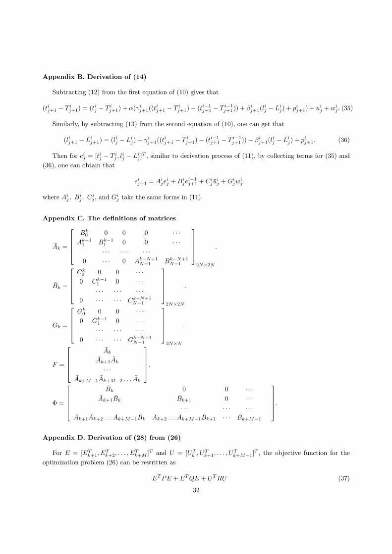
Appendix B. Derivation of (14)

Subtracting (12) from the first equation of (10) gives that

(tij+1 − T ij+1) = (tij − T i

j+1) + α(γij+1((t

ij+1 − T i

j+1)− (ti−1j+1 − T i−1

j+1)) + βij+1(l

ij − Li

j) + pij+1) + uij + wi

j . (35)

Similarly, by subtracting (13) from the second equation of (10), one can get that

(lij+1 − Lij+1) = (lij − Li

j) + γij+1((t

ij+1 − T i

j+1)− (ti−1j+1 − T i−1

j+1))− βij+1(l

ij − Li

j) + pij+1. (36)

Then for eij = [tij − T ij , l

ij − Li

j ]T , similar to derivation process of (11), by collecting terms for (35) and

(36), one can obtain that

eij+1 = Aije

ij +Bi

jei−1j+1 + Ci

j uij +Gi

jwij .

where Aij , Bi

j , Cij , and Gi

j take the same forms in (11).

Appendix C. The definitions of matrices

Ak =

Bk

0 0 0 0 · · ·Ak−1

1 Bk−11 0 0 · · ·· · · · · · · · ·

0 · · · 0 Ak−N+1N−1 Bk−N+1

N−1

2N×2N

.

Bk =

Ck

0 0 0 · · ·0 Ck−1

1 0 · · ·· · · · · · · · ·

0 · · · · · · Ck−N+1N−1

2N×2N

.

Gk =

Gk

0 0 0 · · ·0 Gk−1

1 0 · · ·· · · · · · · · ·

0 · · · · · · Gk−N+1N−1

2N×N

.

F =

Ak

Ak+1Ak

· · ·Ak+M−1Ak+M−2 . . . Ak

.

Φ =

Bk 0 0 · · ·

Ak+1Bk Bk+1 0 · · ·· · · · · · · · ·

Ak+1Ak+2 . . . Ak+M−1Bk Ak+2 . . . Ak+M−1Bk+1 · · · Bk+M−1

.

Appendix D. Derivation of (28) from (26)

For E = [ETk+1, E

Tk+2, . . . , E

Tk+M ]T and U = [UT

k , UTk+1, . . . , U

Tk+M−1]

T , the objective function for the

optimization problem (26) can be rewritten as

ET PE + ET QE + UT RU (37)

32

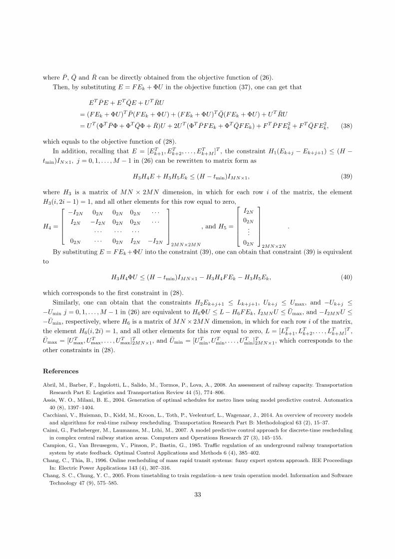
where P , Q and R can be directly obtained from the objective function of (26).

Then, by substituting E = FEk +ΦU in the objective function (37), one can get that

ET PE + ET QE + UT RU

= (FEk +ΦU)T P (FEk +ΦU) + (FEk +ΦU)T Q(FEk +ΦU) + UT RU

= UT (ΦT PΦ+ ΦT QΦ+ R)U + 2UT (ΦT PFEk +ΦT QFEk) + FT PFE2k + FT QFE2

k, (38)

which equals to the objective function of (28).

In addition, recalling that E = [ETk+1, E

Tk+2, . . . , E

Tk+M ]T , the constraint H1(Ek+j − Ek+j+1) ≤ (H −

tmin)IN×1, j = 0, 1, . . . ,M − 1 in (26) can be rewritten to matrix form as

H3H4E +H3H5Ek ≤ (H − tmin)IMN×1, (39)

where H3 is a matrix of MN × 2MN dimension, in which for each row i of the matrix, the element

H3(i, 2i− 1) = 1, and all other elements for this row equal to zero,

H4 =

−I2N 02N 02N 02N · · ·I2N −I2N 02N 02N · · ·

· · · · · · · · ·02N · · · 02N I2N −I2N

2MN×2MN

, and H5 =

I2N

02N...

02N

2MN×2N

.

By substituting E = FEk+ΦU into the constraint (39), one can obtain that constraint (39) is equivalent

to

H3H4ΦU ≤ (H − tmin)IMN×1 −H3H4FEk −H3H5Ek, (40)

which corresponds to the first constraint in (28).

Similarly, one can obtain that the constraints H2Ek+j+1 ≤ Lk+j+1, Uk+j ≤ Umax, and −Uk+j ≤−Umin j = 0, 1, . . . ,M − 1 in (26) are equivalent to H6ΦU ≤ L−H6FEk, I2MNU ≤ Umax, and −I2MNU ≤−Umin, respectively, where H6 is a matrix of MN × 2MN dimension, in which for each row i of the matrix,

the element H6(i, 2i) = 1, and all other elements for this row equal to zero, L = [LTk+1, L

Tk+2, . . . , L

Tk+M ]T ,

Umax = [UTmax, U

Tmax, . . . , U

Tmax]

T2MN×1, and Umin = [UT

min, UTmin, . . . , U

Tmin]

T2MN×1, which corresponds to the

other constraints in (28).

References

Abril, M., Barber, F., Ingolotti, L., Salido, M., Tormos, P., Lova, A., 2008. An assessment of railway capacity. Transportation

Research Part E: Logistics and Transportation Review 44 (5), 774–806.

Assis, W. O., Milani, B. E., 2004. Generation of optimal schedules for metro lines using model predictive control. Automatica

40 (8), 1397–1404.

Cacchiani, V., Huisman, D., Kidd, M., Kroon, L., Toth, P., Veelenturf, L., Wagenaar, J., 2014. An overview of recovery models

and algorithms for real-time railway rescheduling. Transportation Research Part B: Methodological 63 (2), 15–37.

Caimi, G., Fuchsberger, M., Laumanns, M., Lthi, M., 2007. A model predictive control approach for discrete-time rescheduling

in complex central railway station areas. Computers and Operations Research 27 (3), 145–155.

Campion, G., Van Breusegem, V., Pinson, P., Bastin, G., 1985. Traffic regulation of an underground railway transportation

system by state feedback. Optimal Control Applications and Methods 6 (4), 385–402.

Chang, C., Thia, B., 1996. Online rescheduling of mass rapid transit systems: fuzzy expert system approach. IEE Proceedings

In: Electric Power Applications 143 (4), 307–316.

Chang, S. C., Chung, Y. C., 2005. From timetabling to train regulation–a new train operation model. Information and Software

Technology 47 (9), 575–585.

33

Corman, F., D’Ariano, A., Pacciarelli, D., Pranzo, M., 2012. Optimal inter-area coordination of train rescheduling decisions.

Transportation Research Part E 48, 71–88

Cury, J. E., Gomide, F. A. C., Mendes, M. J., 1980. A methodology for generation of optimal schedules for an underground

railway system. IEEE Transactions on Automatic Control 25 (2), 217–222.

Daganzo, C. F., 2009. A headway-based approach to eliminate bus bunching: Systematic analysis and comparisons. Trans-

portation Research Part B: Methodological 43, 913–921.

Daganzo, C. F., Pilachowski, J., 2011. Reducing bunching with bus-to-bus cooperation. Transportation Research Part B:

Methodological 45, 267–277.

Das Gupta, S., Kevin Tobin, J., Pavel, L., 2016. A two-step linear programming model for energy-efficient timetables in metro

railway networks. Transportation Research Part B: Methodological 93, 57–74.

Dundar, S., Sahin, I., 2013. Train re-scheduling with genetic algorithms and artificial neural networks for single-track railways.

Transportation Research Part C: Emerging Technologies 27, 1–15.

Eberlein, X.J., Wilson,N.H.M., Bernstein,D., 2001. The holding problem with real-time information available. Transportation

Science 35(1),1–18.

Fernandez, A., Cucala, A., Vitoriano, B., de Cuadra, F., 2006. Predictive traffic regulation for metro loop lines based on

quadratic programming. Proceedings of the Institution of Mechanical Engineers, Part F: Journal of Rail and Rapid Transit

220 (2), 79–89.

Goodman, C., Murata, S., 2001. Metro traffic regulation from the passenger perspective. Proceedings of the Institution of

Mechanical Engineers, Part F: Journal of Rail and Rapid Transit 215 (2), 137–147.

Haddad, J., Ramezani, M., Geroliminis, N., 2013. Cooperative traffic control of a mixed network with two urban regions and

a freeway. Transportation Research Part B: Methodological 54 (2), 17–36.

Kang, L., Wu, J., Sun, H., Zhu, X., Wang, B., 2015. A practical model for last train rescheduling with train delay in urban

railway transit networks. Omega 50, 29–42.

Le, T., Hai, L. V., Nazarathy, Y., Bao, V., Hoogendoorn, S., 2013. Linear-quadratic model predictive control for urban traffic

networks. Procedia-Social and Behavioral Sciences 80 (11), 512–530.

Li, S. K., De Schutter, B., Yang, L. X., Gao, Z. Y., 2016. Robust model predictive control for train regulation in underground

railway transportation. IEEE Transactions on Control Systems Technology 24 (3), 1075–1083.

Li, X., Hong, K. L., 2014. An energy-efficient scheduling and speed control approach for metro rail operations. Transportation

Research Part B: Methodological 64 (4), 73–89.

Lin, S., De Schutter, B., Xi, Y., Hellendoorn, H., 2011. Fast model predictive control for urban road networks via milp. IEEE

Transactions on Intelligent Transportation Systems 12 (3), 846–856.

Lin, W., Sheu, J., 2010. Automatic train regulation for metro lines using dual heuristic dynamic programming. Proceedings of

the Institution of Mechanical Engineers, Part F: Journal of Rail and Rapid Transit 224 (1), 15–23.

Mannino, C., Mascis, A., 2009. Optimal real-time traffic control in metro stations. Operations Research 57 (4), 1026–1039.

Mayne, D. Q., Rawlings, J. B., Rao, C. V., Scokaert P. O. M., 2000. Constrained model predictive control: Stability and

optimality. Automatica 36, 789–814.

Minciardi, R., Paolucci, M., Presenti, R., 1995. Generating optimal schedules for an underground railway line. Proceedings of

the 34th IEEE Conference on Decision and Control, pp. 4082–4085.

Niu, H., Zhou, X., 2013. Optimizing urban rail timetable under time-dependent demand and oversaturated conditions. Trans-

portation Research Part C: Emerging Technologies 36 (11), 212–230.

Niu, H., Zhou, X., Gao, R., 2015. Train scheduling for minimizing passenger waiting time with time-dependent demand

and skip-stop patterns: Nonlinear integer programming models with linear constraints. Transportation Research Part B:

Methodological 76, 117–135.

Sanchez-Martınez, G., Koutsopoulos, H., Wilson, N., 2016. Real-time holding control for high-frequency transit with dynamics.

Transportation Research Part B: Methodological 83, 1–19.

Sheu, J. W., Lin, W. S., 2012. Energy-saving automatic train regulation using dual heuristic programming. IEEE Transactions

on Vehicular Technology 61 (4), 1503–1514.

Sun, L., Jin, J. G., Lee, D. H., Axhausen, K. W., Erath, A., 2014. Demand-driven timetable design for metro services.

Transportation Research Part C: Emerging Technologies 46, 284–299.

Van Breusegem, V., Campion, G., Bastin, G., 1991. Traffic modeling and state feedback control for metro lines. IEEE Trans-

actions on Automatic Control, 36 (7), 770–784.

Vansteenwegen, P., Oudheusden, D. V., 2004. Developing railway timetables which guarantee a better service. European Journal

of Operational Research 173 (1), 337–350.

Veelenturf, L., Kidd, M., Cacchiani, V., Kroon, L., Toth, P., 2016. A railway timetable rescheduling approach for handling

34

large scale disruptions. Transportation Science 50 (3), 841–862

Xu, X., Li, K., Yang, L., 2016. Rescheduling subway trains by a discrete event model considering service balance performance.

Applied Mathematical Modelling 40 (2), 1446–1466.

Yang, L. X., Zhang, Y., Li, S. K., Gao, Y., 2016. A two-stage stochastic integer programming model or the transfer activity

choice in metro networks. Transportation Research Part B: Methodological 83, 271–297.

Yin, J., Tang, T., Yang, L., Gao, Z., Ran, B., 2016. Energy-efficient metro train rescheduling with uncertain time-variant

passenger demands: An approximate dynamic programming approach. Transportation Research Part B: Methodological 91,

178–210.

Yin, J., Yang, L., Tang, T., Gao, Z., Ran, B., 2017. Dynamic passenger demand oriented metro train scheduling with energy-

efficiency and waiting time minimization: Mixed-integer linear programming approaches. Transportation Research Part B:

Methodological 97, 182–213.

35