Josef Matous Kristin Y. Pettersen Claudio Paliottaˇ

Formation Path Following Control of Underactuated AUVs – WithProofs

Josef Matous Kristin Y. Pettersen Claudio Paliotta

Abstract— This paper proposes a novel method for formationpath following of multiple underactuated autonomous underwa-ter vehicles. The method combines line-of-sight guidance withnull-space-based behavioral control, allowing the vehicles tofollow curved paths while maintaining the desired formation.We investigate the dynamics of the path-following error usingcascaded systems theory, and show that the closed-loop systemis uniformly semi-globally exponentially stable. We validate thetheoretical results through numerical simulations.

I. INTRODUCTION

Autonomous underwater vehicles (AUVs) are being in-creasingly used in a number of applications such as trans-portation, seafloor mapping, and in the ocean energy industry.Some complex tasks need to be performed by a group ofcooperating AUVs. Consequently, there is a need for controlalgorithms that can guide a formation of AUVs along a givenpath while avoiding collisions with each other.

A comprehensive overview of various formation path-following methods is presented in [1]. Most of these methodsare based on two concepts: coordinated path-following [2],[3], and leader-follower [4], [5]. In the coordinated path-following approach, each vehicle follows a predefined pathseparately. Formation is then achieved by coordinating themotion of the vehicles along these paths. In this approach,the formation-keeping error (i.e., the difference between theactual and desired relative position of the vessels) mayinitially grow as the vehicles converge to their predefinedpaths. In the leader-follower approach, one leading vehiclefollows the given path while the followers adjust their speedand position to obtain the desired formation shape. Thisapproach tends to suffer from the lack of formation feedbackdue to the unidirectional communication (i.e., the leader doesnot adjust its velocity based on the followers).

The null-space-based behavioral (NSB) algorithm has alsobeen proposed to solve the formation path-following prob-lem [6]–[9]. The NSB algorithm is a centralized controlmethod that allows to combine several hierarchic tasks.In the NSB framework, it is possible to design the path-following, formation-keeping and collision avoidance tasksindependently. By combining these tasks, the vehicles exhibitthe desired behavior.

This paper aims to extend the results of [9], where an NSBalgorithm is used to guide two surface vessels moving in the

Josef Matous and Kristin Y. Pettersen are with the Centre for AutonomousMarine Operations and Systems, Department of Engineering Cybernetics,Norwegian University of Science and Technology (NTNU), Trondheim,Norway. josef.matous, [email protected] Paliotta is with SINTEF Digital, Trondheim, [email protected]

horizontal plane. Specifically, we propose an algorithm thatworks with an arbitrary number of AUVs with five degrees offreedom (DOFs) moving in 3D. Similarly to [9], we solve thepath-following task using line-of-sight (LOS) guidance. Us-ing the cascaded systems theory results of [10], we prove thatthe closed-loop system consisting of a 3D LOS guidance law,combined with surge, pitch and yaw autopilots based on [11],is uniformly semi-globally exponentially stable (USGES)and uniformly globally asymptotically stable (UGAS). Thetheoretical results are verified through numerical simulations.

The remainder of the paper is organized as follows.Section II introduces the model of the AUVs. In Section III,we define the formation path-following problem. In SectionIV, we describe the control system. The stability of thecontrol system is proven in Section V. Section VI containsthe results of a numerical simulation. Finally, Section VIIcontains some concluding remarks.

II. MODEL

In this section, we present the model of the AUV. We startby introducing the model in a matrix-vector form. Then, wewrite out the ordinary differential equations (ODEs) for theindividual state variables.

A. Vessel Model in Vector-Matrix Form

The pose (η) and velocities (ν) of an AUV with 5DOFsare defined as

η = [x, y, z, θ, ψ]T, ν = [u, v, w, q, r]

T, (1)

where x, y, z are the coordinates of the vessel in North-East-Down (NED) coordinate frame, and θ and ψ are the pitch andyaw angles, respectively. The velocities u, v, w are the linearsurge, sway and heave velocities in a given body-fixed frame,and q and r are the pitch and yaw rate, respectively. The rolldynamics are disregarded as the roll motion is assumed tobe small and self-stabilizing by the vehicle design.

Let Vc = [Vx, Vy, Vz]T be the velocities of an unknown,

constant and irrotational ocean current, given in the inertialNED frame. Let J (η) be the transformation matrix from thebody-fixed to the inertial frame. J (η) is given by

J (η) =

[R (θ, ψ) O3×3

O3×3 T (θ)

], (2)

where R (θ, ψ) is the rotation matrix from the body-fixed tothe inertial coordinate frames, O3×3 is a 3-by-3 matrix ofzeros, and T (θ) = diag(1, 1/ cos θ), which is well-defined ifthe pitch angle |θ| < π/2. Note that the mechanical design of

arX

iv:2

111.

0345

5v1

[ee

ss.S

Y]

5 N

ov 2

021

torpedo-shaped rudder-controlled AUVs generally does notallow for pitch angles |θ| = π/2.

The velocities of the ocean current expressed in the body-fixed coordinate frame, νc, are thus

νc =

[(R (θ, ψ)

TVc

)T

, 0, 0

]T

. (3)

We will denote the relative velocities of the vessel as νr =ν − νc. We will also denote the relative surge, sway andheave velocities as ur, vr and wr, respectively.

Let f = [Tu, δe, δr] be the vector of control inputs, whereTu is the surge thrust generated by the propeller, and δeand δr are the deflection angles of the elevator and rudder,respectively. Furthermore, let M be the mass and inertiamatrix, including added mass effects, C (νr) the Corioliscentripetal matrix, also including added mass effects, andD (νr) the hydrodynamic damping matrix. The dynamics ofthe vessel in a matrix-vector form are then [12]

η = J (η)ν, (4)Mνr + C (νr)νr + D (νr)νr + g (η) = Bf , (5)

where g (η) is the gravity and buoyancy vector, and B is theactuator configuration matrix that maps the control inputs toforces and torques.

B. Vessel Model in Component Form

First, let us present the necessary assumptions for derivingthe ODEs for individual state variables.

Assumption 1: The vessel is slender, torpedo-shaped withport-starboard symmetry.

Assumption 2: The vessel is maneuvering at low speeds.Consequently, the nonlinear hydrodynamic damping matrixcan be approximated by a constant matrix.

Assumption 3: The vessel is neutrally buoyant with thecenter of gravity (CG) and the center of buoyancy (CB)located along the same vertical axis.

Under these assumptions, the M and B matrices have thefollowing form

M=

m11 0 0 0 0

0 m22 0 0 m25

0 0 m33 m34 00 0 m34 m44 00 m25 0 0 m55

, B=

b11 0 00 0 b23

0 b32 00 b42 00 0 b53

(6)

the corresponding Coriolis matrix is

C (νr) =

0 0 0 c1 −c20 0 0 0 c30 0 0 −c3 0−c1 0 c3 0 0c2 −c3 0 0 0

, (7)

where c1 = m34 q + m33 wr, c2 = m25 r + m22 vr, and

c3 = m11 ur. The hydrodynamic damping matrix is

D (νr) ≈ D =

d11 0 0 0 00 d22 0 0 d25

0 0 d33 d34 00 0 d43 d44 00 d52 0 0 d55

, (8)

and the gravity vector has the following form

g (η) = [0, 0, 0,m g zg sin(θ)]T, (9)

where m is the weight of the vessel, g is the gravityacceleration, and zg is the vertical distance between the CGand CB [12].

Furthermore, it can be shown [13] that there is a changeof coordinates such that

M−1 B f = [fu, 0, 0, tq, tr]T. (10)

Let us assume that we have a model for which (10) andAssumptions 1–3 hold. Then, the model in component formis

x = u cos (ψ) cos (θ)− v sin (ψ) + w cos (ψ) sin (θ) , (11a)y = u cos (θ) sin (ψ) + v cos (ψ) + w sin (ψ) sin (θ) , (11b)z = −u sin (θ) + w cos (θ) , (11c)

θ = q, (11d)

ψ = 1cos(θ) r, (11e)

u = fu + Fu(u, v, w, q, r) + φu(u, v, w, q, r, θ, ψ)T Vc, (11f)v = Xv(u, uc) r + Yv(u, uc) vr, (11g)w = Xw(u, uc) q + Yw(u, uc)wr +G(θ), (11h)q = tq + Fq(u,w, q, θ) + φq(u,w, q, θ, ψ)T ϑ (Vc) , (11i)r = tr + Fr(u, v, r) + φr(u, v, r, θ, ψ)T ϑ (Vc) , (11j)

where ϑ (Vc) =[Vx, Vy, Vz, V

2x , V

2y , V

2z , Vx Vy, Vx Vz, Vy Vz

]T,and the expressions for Fi(·), φi(·), i ∈ u, q, r, Xv(·),Yv(·), Xw(·), Yw(·), and G(·) are given in Appendix I.

III. CONTROL OBJECTIVES

The goal is to control n AUVs so that they move ina prescribed formation while avoiding collisions and theirbarycenter follows a given path.

The prescribed path in the inertial coordinate frame isgiven by a smooth function pp : R → R3. We assumethat the path function is C2 and regular, i.e., the function iscontinuous up to its second derivative and its first derivativewith respect to the path parameter satisfies∥∥∥∥∂pp(ξ)

∂ξ

∥∥∥∥ 6= 0. (12)

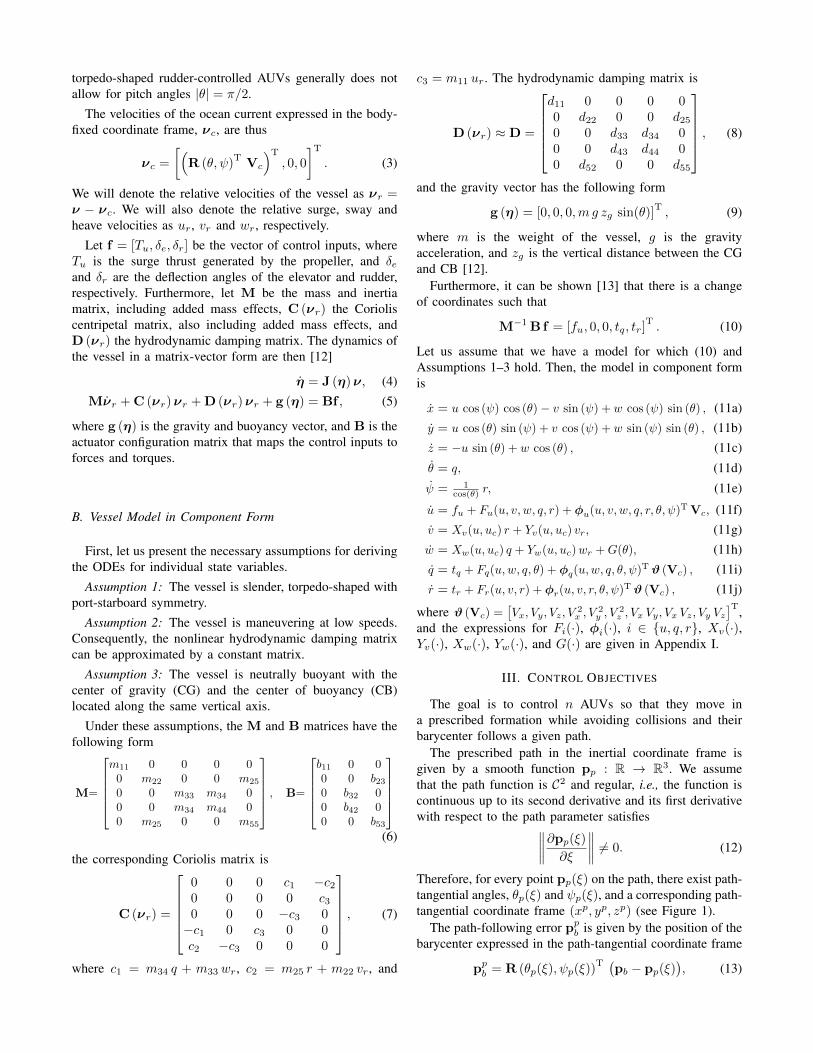
Therefore, for every point pp(ξ) on the path, there exist path-tangential angles, θp(ξ) and ψp(ξ), and a corresponding path-tangential coordinate frame (xp, yp, zp) (see Figure 1).

The path-following error ppb is given by the position of thebarycenter expressed in the path-tangential coordinate frame

ppb = R (θp(ξ), ψp(ξ))T (

pb − pp(ξ)), (13)

x

y

z

xp

yp

zp

pp(ξ)

ψp(ξ) θp(ξ)

Fig. 1. Definition of the path angles and path-tangential coordinate frame.The grey line represents the projection of the path-tangential vector into thexy-plane

where

pb =1

n

n∑i=1

pi, pi = [xi, yi, zi]T, (14)

where (xi, yi, zi) is the position of the ith vessel. The goalof path following is to control the vessels so that ppb ≡ 03,where 03 is a 3-element vector of zeros.

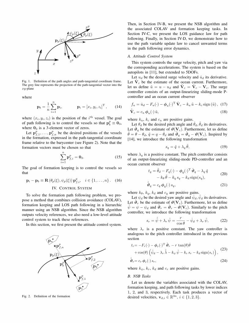
Let ppf,1, . . . ,ppf,n be the desired positions of the vessels

in the formation, expressed in the path-tangential coordinateframe relative to the barycenter (see Figure 2). Note that theformation vectors must be chosen so that

n∑i=1

ppf,i = 03. (15)

The goal of formation keeping is to control the vessels sothat

pi − pb ≡ R (θp(ξ), ψp(ξ)) ppf,i, i ∈ 1, . . . , n . (16)

IV. CONTROL SYSTEM

To solve the formation path following problem, we pro-pose a method that combines collision avoidance (COLAV),formation keeping and LOS path following in a hierarchicmanner using an NSB algorithm. Since the NSB algorithmoutputs velocity references, we also need a low-level attitudecontrol system to track these references.

In this section, we first present the attitude control system.

pp(ξ)

ppb

ppf,1

ppf,2

ppf,n

p1

p2

pn

Fig. 2. Definition of the formation

Then, in Section IV-B, we present the NSB algorithm andthe associated COLAV and formation keeping tasks. InSection IV-C, we present the LOS guidance law for pathfollowing. Finally, in Section IV-D, we demonstrate how touse the path variable update law to cancel unwanted termsin the path following error dynamics.

A. Attitude Control System

This system controls the surge velocity, pitch and yaw viathe corresponding accelerations. The system is based on theautopilots in [11], but extended to 5DOFs.

Let ud be the desired surge velocity and ud its derivative.Let Vc be the estimate of the ocean current. Furthermore,let us define u = u − ud and Vc = Vc − Vc. The surgecontroller consists of an output-linearizing sliding-mode P-controller and an ocean current observer

fu = ud − Fu(·)− φu(·)T Vc − ku u− kc sign (u) , (17)˙Vc = cu φu(·) u, (18)

where ku, kc and cu are positive gains.Let θd be the desired pitch angle and θd, θd its derivatives.

Let ϑq be the estimate of ϑ(Vc). Furthermore, let us defineθ = θ − θd, q = q − θd and ϑq = ϑq − ϑ(Vc). Inspired by[14], we introduce the following transformation

sq = q + λq θ, (19)

where λq is a positive constant. The pitch controller consistsof an output-linearizing sliding-mode PD-controller and anocean current observer

tq = θd − Fq(·)− φq(·)T ϑq − λq q− kθ θ − kq sq − kd sign(sq),

(20)

˙ϑq = cq φq(·) sq, (21)

where kθ, kq , kd and cq are positive gains.Let ψd be the desired yaw angle and ψd, ψd its derivatives.

Let ϑr be the estimate of ϑ(Vc). Furthermore, let us defineψ = ψ − ψd and ϑr = ϑr − ϑ(Vc). Similarly to the pitchcontroller, we introduce the following transformation

sr =˙ψ + λr ψ =

r

cos θ− ψd + λr ψ, (22)

where λr is a positive constant. The yaw controller isanalogous to the pitch controller introduced in the previoussection

tr= −Fr(·)− φr(·)T ϑr − r tan(θ)θ

+ cos(θ)(ψd − λr ˙

λ− kψ ψ − kr sr − kd sign(sr)),

(23)

˙ϑr= cr φr(·) sr, (24)

where kψ , kr, kd and cr are positive gains.

B. NSB Tasks

Let us denote the variables associated with the COLAV,formation keeping, and path following tasks by lower indices1, 2, and 3, respectively. Each task produces a vector ofdesired velocities, vd,i ∈ R3n, i ∈ 1, 2, 3.

For the COLAV and formation keeping tasks, the desiredvelocities are obtained using task varibles, σ1 and σ2, andtheir desired values, σd,1 and σd,2.

First, let us consider the COLAV task. Let dCOLAV be theactivation distance, i.e., the distance at which the vesselsneed to start performing the evasive maneuvers to avoidcollision. The task variable is then given by a vector ofrelative distances between the vessels smaller than dCOLAV,i.e.,

σ1 =[‖pi − pj‖

]T,∀i, j ∈ 1, . . . , n, j > i,

‖pi − pj‖ < dCOLAV.(25)

The desired values of the task are

σ1,d = dCOLAV 1, (26)

where 1 is a vector of ones.Now, let us consider the formation keeping task. The task

variable is defined as

σ2 =[σT

2,1, . . . ,σT2,n−1

]T, σ2,i = pi − pb, (27)

and its desired values are

σd,2 =

R (θp(ξ), ψp(ξ)) ppf,1...

R (θp(ξ), ψp(ξ)) ppf,n−1

. (28)

The desired velocities of the COLAV and formationkeeping tasks are obtained using the closed-loop inversekinematics (CLIK) equation [6]

vd,i = J†i (σd,i −Λi σi) , i ∈ 1, 2, (29)

where σi = σi −σd,i is the error, J† is the Moore-Penrosepseudoinverse given by

J† = JT(J JT

)−1

, (30)

Λi is a positive definite gain matrix, and Ji is the taskJacobian given by

Ji =∂σi∂p

, p =[pT

1 , . . . ,pTn

]T. (31)

The desired velocity of the path-following task is obtainedusing LOS guidance that is explained in the next section.These velocities are then combined using the NSB algorithm

vNSB = vd,1 +(I− J†1J1

)(vd,2 +

(I− J†2J2

)vd,3

), (32)

if there are active COLAV tasks, and

vNSB = vd,2 +(I− J†2J2

)vd,3, (33)

if there are none (I is an identity matrix). The NSB velocitiesmust be decomposed into surge, pitch and yaw referencesthat can be tracked by the attitude control system presentedin Section IV-A. Similarly to [6], we propose a method withangle of attack and sideslip compensation

ud,i= UNSB,i1+cos(γNSB,i−γi) cos(χNSB,i−χi)

2 , (34)

θd,i= γNSB,i + αd,i, αd,i = arctan(wiud,i

), (35)

ψd,i= χNSB,i − βd,i, βd,i = arcsin

(vi√

u2d,i+v

2i+w2

i

), (36)

where vi and wi are the sway and heave velocities, and γiand χi are the flight-path and course angles of the ith vessel,respectively, and UNSB,i, γNSB,i and χNSB,i are given by

UNSB,i = ‖vNSB,i‖ , vNSB,i =

xNSB,i

yNSB,i

zNSB,i

, (37a)

γNSB,i = − arcsin

(yNSB,i

UNSB,i

), (37b)

χNSB,i = arctan2 (yNSB,i, xNSB,i) , (37c)

where arctan2(y, x) is the four-quadrant inverse tan.

C. Line-of-Sight Guidance

The desired flight-path angle and course of the path-following task are given by the following LOS law

γLOS= θp(ξ) + arctan

(zpb

∆(ppb)

), (38)

χLOS= ψp(ξ)− arctan

(ypb

∆(ppb)

), (39)

where ppb = [xpb , ypb , z

pb ]

T, and ∆ (ppb) is the lookaheaddistance. Inspired by [15], we choose the lookahead distanceas

∆ (ppb) =

√∆2

0 + (xpb)2

+ (ypb )2

+ (zpb )2, (40)

where ∆0 > 0 is a constant.

The desired velocity of the path-following task is thengiven by

vd,3 = 1n ⊗ vLOS, (41)

where · ⊗ · is the Kronecker tensor product, and

vLOS =

cos (χLOS) cos (γLOS)cos (γLOS) sin (χLOS)− sin (γLOS)

ULOS, (42)

where ULOS is the desired path-following speed.

D. Path Parametrization

Inspired by [15], we use the update law of the path variableξ to get desirable behavior of the along-track error (xpb ).

Note that the kinematics of the ith vessel can be alterna-tively expressed using the total speed (Ui) and the flight-path(γi) and course (χi) angles of the vessel as

pi = [cos (χi) cos (γi) , cos (γi) sin (χi) , − sin (γi)]TUi. (43)

Now, let us investigate the kinematics of the barycenter.Differentiating (13) with respect to time and substituting (43)

yields the following equations

xpb =1

n

n∑i=1

Ui Ωx (γi, θp, χi, ψp)

−∥∥∥∂pp(ξ)

∂ξ

∥∥∥ξ + ωzypb − ωyz

pb ,

(44a)

ypb =1

n

n∑i=1

Ui Ωy (γi, θp, χi, ψp) + ωxzpb − ωzx

pb , (44b)

zpb =1

n

n∑i=1

Ui Ωz (γi, θp, χi, ψp) + ωyxpb − ωxy

pb , (44c)

where

Ωx(·)= sin (θp) sin (γi) + cos (θp) cos (γi) cos (ψp − χi) , (45a)Ωy(·)= − cos (γi) sin (ψp − χi) , (45b)Ωz(·)= − cos (θp) sin (γi) + cos (γi) sin(θp) cos (ψp − χi)(45c)ωx= −ιξ sin(θp), ωy= κξ, ωz= ιξ cos(θp), (45d)

κ(ξ)=∂θp(ξ)∂ξ , ι(ξ)=

∂ψp(ξ)∂ξ . (45e)

To stabilize the along-track error dynamics, we choose thefollowing path variable update law

ξ =

∥∥∥∥∂pp(ξ)

∂ξ

∥∥∥∥−1(

1

n

n∑i=1

Ui Ωx (γi, θp, χi, ψp)

+kξxpb√

1 + (xpb)2

,

(46)

where kξ > 0 is a constant.

V. CLOSED-LOOP ANALYSIS

In this section, we investigate the closed-loop stability ofthe path following task. We define two error states, X1 andX2, as

X1 = [xpb , ypb , z

pb ]

T, X2 =

[XT

2,1, . . . , XT2,n

]T, (47)

X2,i =[ui, sq,i, θi, sr,i, ψi

]T, (48)

Now, we can take the barycenter kinematics from (44) andexpress it in terms of X1 and X2 as

xpb = −kξxpb√

1 + (xpb)2

+ ωzypb − ωyz

pb , (49a)

ypb = − 1

n

n∑i=1

Ud,icos (γLOS) ypb√∆ (ppb)

2+ (ypb )

2+ ωxz

pb − ωzx

pb

+Gy(u1, . . . , un, ψ1, . . . , ψn, γ1, . . . , γn,

ud,1, . . . , ud,n, v1, . . . , vn, w1, . . . , wn,ppb , ψp

),

(49b)

zpb =1

n

n∑i=1

Ud,izpb√

∆ (ppb)2

+ (zpb )2

+ ωyxpb − ωxy

pb

+Gz(u1, . . . , un, θ1, . . . , θn, γ1, . . . , γn, χ1, . . . , χn,

ud,1, . . . , ud,n, v1, . . . , vn, w1, . . . , wn,ppb , ψp, θp

).

(49c)

The equations for Gy(·) and Gz(·) are given in Appendix II-A. Substituting the attitude control system (17)–(24) into ves-sel dynamics (11) yields the following closed-loop behaviorof X2

˙ui = −ku ui − kc sign (ui)− φu(·)TVc,i, (50a)

sq,i = −kθ θi − kq sq,i − kd sign(sq,i)− φq(·)T ϑq,i, (50b)˙θi = sq,i − λq θi, (50c)

sr,i = −kθ θi − kr sr,i − kd sign(sr,i)− φr(·)T ϑr,i, (50d)˙ψi = sr,i − λr ψi, (50e)

the ocean current estimate errors˙Vc,i = cu φu(·) ui, (51a)˙ϑq,i = cq φq(·) sq,i, (51b)˙ϑr,i = cr φr(·) sr,i, (51c)

and the underactuated sway and heave dynamics

vi = Xv(ui, uc) ri + Yv(ui, uc) (vi − vc), (52)wi = Xw(ui, uc) qi + Yw(ui, uc) (wi − wc) +G(θi). (53)

To prove the stability of the closed-loop system, we needthe results of the three following lemmas. The lemmas followthe same structure as the 2D case for two ASVs in [9], andare extended to handle an arbitrary number of AUVs movingin 3D.

Lemma 1: The trajectories of the closed-loop system(49)–(53) are forward complete.

Proof: The proof is given in Appendix II-C.Lemma 2: The underactuated sway and heave dynam-

ics are bounded near the manifold[XT

1 , XT2

]= 0T if

Yv(u, uc) < 0, Yw(u, uc) < 0 and the curvature of the pathsatisfies

|κ(ξ)| < n

2

∣∣∣∣ Yw(u, uc)

Xw(u, uc)

∣∣∣∣ , |ι(ξ)| < n

2

∣∣∣∣ Yv(u, uc)Xv(u, uc)

∣∣∣∣ , (54)

for all u > 0 and uc ∈ [−‖Vc‖ , ‖Vc‖].Proof: The proof is given in Appendix II-D.

Lemma 3: The underactuated sway and heave dynamicsare bounded near the manifold X2 = 0, independently ofX1 if the assumptions in Lemma 2 are satisfied and theconstant term ∆0 in the lookahead distance (40) is chosenso that

∆0 > max

3

n∣∣∣ Yv(u,uc)Xv(u,uc)

∣∣∣− 2 |ι(ξ)|,

3

n∣∣∣ Yw(u,uc)Xw(u,uc)

∣∣∣− 2 |κ(ξ)|

,

(55)

for all u > 0 and uc ∈ [−‖Vc‖ , ‖Vc‖].Proof: The proof is given in Appendix II-E.

Theorem 1: The origin[XT

1 , XT2

]= 0T of the system

described by (49),(50) is a USGES equilibrium point if theconditions of Lemmas 2 and 3 hold and the maximum pitch

angle of the path satisfies

θp,max = maxξ∈R|θp(ξ)| <

π

4. (56)

Moreover, the ocean current estimate errors (51) and the un-deractuated sway and heave dynamics (52), (53) are bounded.

Remark: Condition (56) is needed to ensure that |γLOS| <π/2. Indeed, from (38), the largest possible LOS referenceangle is

γLOS,max = θp,max + limzpb→∞

arctan

(zpb√

∆20+(zpb )

2

)= θp,max +

π

4.

(57)

With (56) satisfied, the cosine of γLOS is always positive.We will use this fact in the proof.

Proof: The proof follows along the lines of [9], butis extended to an arbitrary number of 5DOF vessels. Wewill also use the results of [10] to prove that the system isUSGES.

In Lemmas 1–3, we have shown that the closed-loopsystem is forward complete and the underactuated sway andheave dynamics are bounded near the manifold X2 = 0.Since (50) is UGES [11], we can conclude that there existsa finite time T > t0 such that the solutions of (50) willbe sufficiently close to X2 = 0 to guarantee boundednessof vi and wi. Having established that the underactuateddynamics are bounded, we will now utilize cascaded theoryto analyze the cascade (49), (50), where (50) perturbs thenominal dynamics (49) through the terms Gy(·) and Gz(·).

Now, consider the nominal dynamics of X1 (i.e., (49)without the perturbing terms Gy and Gz), and a Lyapunovfunction candidate

V (X1) =1

2XT

1 X1 =1

2

((xpb)

2 + (ypb )2 + (zpb )2), (58)

whose derivative along the trajectories of (49) is

V (X1) = −XT1 Q X1, Q = diag(q1, q2, q3), (59a)

q1 =kξ√

1+(xpb)2, q2 =

1n

∑ni=1 Ud,i cos(γLOS)√∆(ppb)

2+(ypb )

2, (59b)

q3 =1n

∑ni=1 Ud,i√

∆(ppb)2+(zpb )

2. (59c)

Note that Q is positive definite, and the nominal system isthus UGAS. Furthermore, note that the following inequality

V (X1) ≤ −qmin

∥∥∥X1

∥∥∥2

, (60a)

qmin = min

kξ√1+r2

,1n

∑ni=1 Ud,i cos(γLOS)√

∆20+4r2

, (60b)

holds ∀X1 ∈ Br. Thus, the conditions of [10, Theorem 5]are fulfilled with k1 = k2 = 1/2, a = 2, and k3 = qmin, andthe nominal system is USGES.

As discussed in the proof of Lemma 1, the perturbingsystem (50) is UGES, implying both UGAS and USGES.Furthermore, it is straightforward to show that the following

holds for the Lyapunov function (58)∥∥∥∥ ∂V∂X1

∥∥∥∥ ∥∥∥X1

∥∥∥ =∥∥∥X1

∥∥∥2

= 2V(X1

), ∀X1, (61)∥∥∥∥ ∂V∂X1

∥∥∥∥ =∥∥∥X1

∥∥∥ ≤ µ, ∀∥∥∥X1

∥∥∥ ≤ µ. (62)

Therefore, [10, Assumption 1] is satisfied with c1 = 2 andc2 = µ for any µ > 0.

Finally, [10, Assumption 2] must be investigated. From(79), (89), it can be shown that for both perturbing termsthere exist positive functions ζy,1(·), ζy,2(·), ζz,1(·), ζz,2(·),such that

|Gy(·)| ≤ ζy,1(∥∥∥X2

∥∥∥) + ζy,2(∥∥∥X2

∥∥∥)∥∥∥X1

∥∥∥ , (63)

|Gz(·)| ≤ ζz,1(∥∥∥X2

∥∥∥) + ζz,2(∥∥∥X2

∥∥∥)∥∥∥X1

∥∥∥ . (64)

Therefore, all conditions of [10, Proposition 9] are satisfied,and the closed-loop system is USGES.

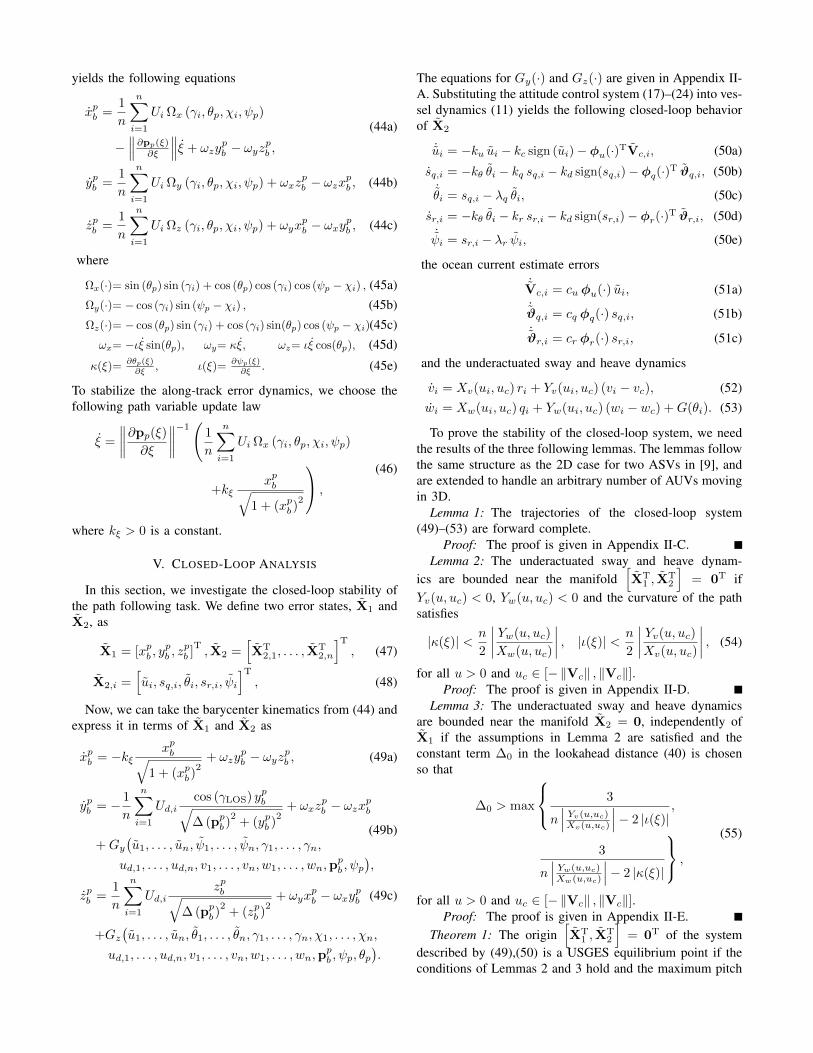
VI. SIMULATION

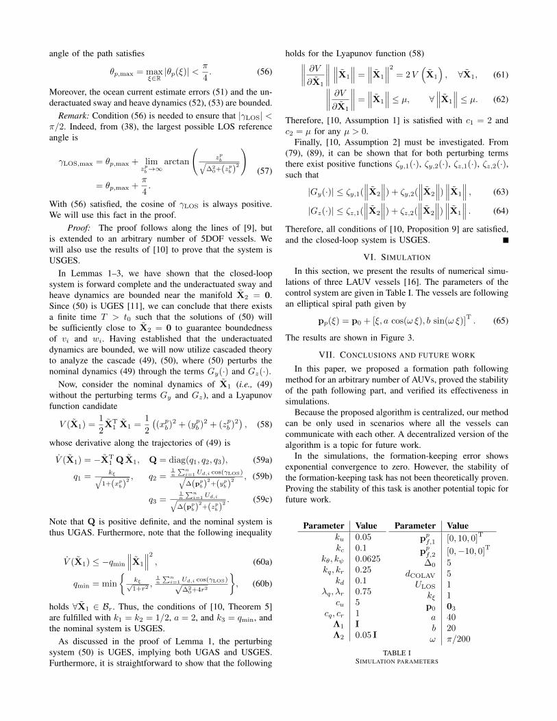
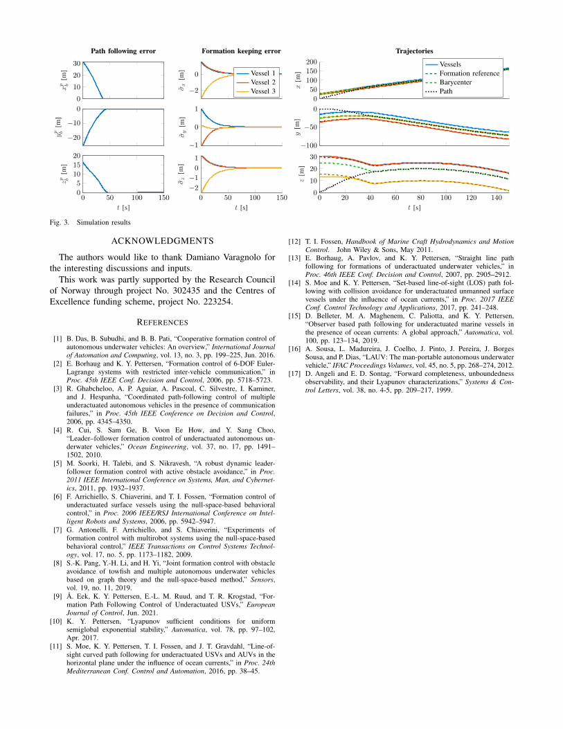
In this section, we present the results of numerical simu-lations of three LAUV vessels [16]. The parameters of thecontrol system are given in Table I. The vessels are followingan elliptical spiral path given by

pp(ξ) = p0 + [ξ, a cos(ω ξ), b sin(ω ξ)]T. (65)

The results are shown in Figure 3.

VII. CONCLUSIONS AND FUTURE WORK

In this paper, we proposed a formation path followingmethod for an arbitrary number of AUVs, proved the stabilityof the path following part, and verified its effectiveness insimulations.

Because the proposed algorithm is centralized, our methodcan be only used in scenarios where all the vessels cancommunicate with each other. A decentralized version of thealgorithm is a topic for future work.

In the simulations, the formation-keeping error showsexponential convergence to zero. However, the stability ofthe formation-keeping task has not been theoretically proven.Proving the stability of this task is another potential topic forfuture work.

Parameter Valueku 0.05kc 0.1

kθ, kψ 0.0625kq, kr 0.25

kd 0.1λq, λr 0.75

cu 5cq, cr 1

Λ1 IΛ2 0.05 I

Parameter Valueppf,1 [0, 10, 0]

T

ppf,2 [0,−10, 0]T

∆0 5dCOLAV 5ULOS 1

kξ 1p0 03

a 40b 20ω π/200

TABLE ISIMULATION PARAMETERS

0

10

20

30xp b

[m]

Path following error

−20

−10

0

yp b

[m]

0 50 100 1500

5

10

15

20

t [s]

zp b

[m]

−2

0

σx

[m]

Formation keeping error

Vessel 1Vessel 2Vessel 3

−1

0

1

σy

[m]

0 50 100 150

−2

−1

0

1

t [s]

σz

[m]

0

50

100

150

200

x[m

]

Trajectories

VesselsFormation referenceBarycenterPath

−100

−50

0

y[m

]

0 20 40 60 80 100 120 1400

10

20

30

t [s]

z[m

]

Fig. 3. Simulation results

ACKNOWLEDGMENTS

The authors would like to thank Damiano Varagnolo forthe interesting discussions and inputs.

This work was partly supported by the Research Councilof Norway through project No. 302435 and the Centres ofExcellence funding scheme, project No. 223254.

REFERENCES

[1] B. Das, B. Subudhi, and B. B. Pati, “Cooperative formation control ofautonomous underwater vehicles: An overview,” International Journalof Automation and Computing, vol. 13, no. 3, pp. 199–225, Jun. 2016.

[2] E. Borhaug and K. Y. Pettersen, “Formation control of 6-DOF Euler-Lagrange systems with restricted inter-vehicle communication,” inProc. 45th IEEE Conf. Decision and Control, 2006, pp. 5718–5723.

[3] R. Ghabcheloo, A. P. Aguiar, A. Pascoal, C. Silvestre, I. Kaminer,and J. Hespanha, “Coordinated path-following control of multipleunderactuated autonomous vehicles in the presence of communicationfailures,” in Proc. 45th IEEE Conference on Decision and Control,2006, pp. 4345–4350.

[4] R. Cui, S. Sam Ge, B. Voon Ee How, and Y. Sang Choo,“Leader–follower formation control of underactuated autonomous un-derwater vehicles,” Ocean Engineering, vol. 37, no. 17, pp. 1491–1502, 2010.

[5] M. Soorki, H. Talebi, and S. Nikravesh, “A robust dynamic leader-follower formation control with active obstacle avoidance,” in Proc.2011 IEEE International Conference on Systems, Man, and Cybernet-ics, 2011, pp. 1932–1937.

[6] F. Arrichiello, S. Chiaverini, and T. I. Fossen, “Formation control ofunderactuated surface vessels using the null-space-based behavioralcontrol,” in Proc. 2006 IEEE/RSJ International Conference on Intel-ligent Robots and Systems, 2006, pp. 5942–5947.

[7] G. Antonelli, F. Arrichiello, and S. Chiaverini, “Experiments offormation control with multirobot systems using the null-space-basedbehavioral control,” IEEE Transactions on Control Systems Technol-ogy, vol. 17, no. 5, pp. 1173–1182, 2009.

[8] S.-K. Pang, Y.-H. Li, and H. Yi, “Joint formation control with obstacleavoidance of towfish and multiple autonomous underwater vehiclesbased on graph theory and the null-space-based method,” Sensors,vol. 19, no. 11, 2019.

[9] A. Eek, K. Y. Pettersen, E.-L. M. Ruud, and T. R. Krogstad, “For-mation Path Following Control of Underactuated USVs,” EuropeanJournal of Control, Jun. 2021.

[10] K. Y. Pettersen, “Lyapunov sufficient conditions for uniformsemiglobal exponential stability,” Automatica, vol. 78, pp. 97–102,Apr. 2017.

[11] S. Moe, K. Y. Pettersen, T. I. Fossen, and J. T. Gravdahl, “Line-of-sight curved path following for underactuated USVs and AUVs in thehorizontal plane under the influence of ocean currents,” in Proc. 24thMediterranean Conf. Control and Automation, 2016, pp. 38–45.

[12] T. I. Fossen, Handbook of Marine Craft Hydrodynamics and MotionControl. John Wiley & Sons, May 2011.

[13] E. Borhaug, A. Pavlov, and K. Y. Pettersen, “Straight line pathfollowing for formations of underactuated underwater vehicles,” inProc. 46th IEEE Conf. Decision and Control, 2007, pp. 2905–2912.

[14] S. Moe and K. Y. Pettersen, “Set-based line-of-sight (LOS) path fol-lowing with collision avoidance for underactuated unmanned surfacevessels under the influence of ocean currents,” in Proc. 2017 IEEEConf. Control Technology and Applications, 2017, pp. 241–248.

[15] D. Belleter, M. A. Maghenem, C. Paliotta, and K. Y. Pettersen,“Observer based path following for underactuated marine vessels inthe presence of ocean currents: A global approach,” Automatica, vol.100, pp. 123–134, 2019.

[16] A. Sousa, L. Madureira, J. Coelho, J. Pinto, J. Pereira, J. BorgesSousa, and P. Dias, “LAUV: The man-portable autonomous underwatervehicle,” IFAC Proceedings Volumes, vol. 45, no. 5, pp. 268–274, 2012.

[17] D. Angeli and E. D. Sontag, “Forward completeness, unboundednessobservability, and their Lyapunov characterizations,” Systems & Con-trol Letters, vol. 38, no. 4-5, pp. 209–217, 1999.

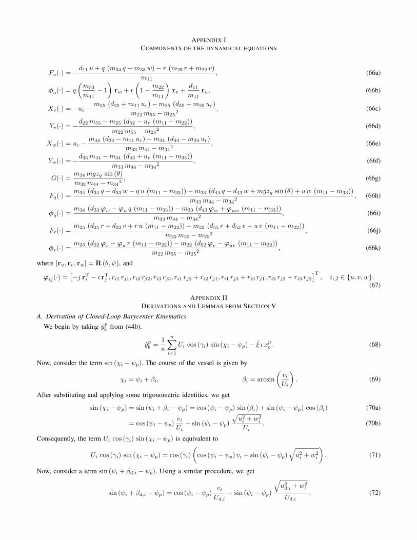
APPENDIX ICOMPONENTS OF THE DYNAMICAL EQUATIONS

Fu(·) = −d11 u+ q (m34 q +m33 w)− r (m25 r +m22 v)

m11, (66a)

φu(·) = q

(m33

m11− 1

)rw + r

(1− m22

m11

)rv +

d11

m11ru, (66b)

Xv(·) = −uc −m55 (d25 +m11 ur)−m25 (d55 +m25 ur)

m22m55 −m252

, (66c)

Yv(·) = −d22m55 −m25 (d52 − ur (m11 −m22))

m22m55 −m252

, (66d)

Xw(·) = uc −m44 (d34 −m11 ur)−m34 (d44 −m34 ur)

m33m44 −m342

, (66e)

Yw(·) = −d33m44 −m34 (d43 + ur (m11 −m33))

m33m44 −m342

, (66f)

G(·) =m34mgzg sin (θ)

m33m44 −m342, (66g)

Fq(·) =m34 (d34 q + d33 w − q u (m11 −m33))−m33 (d44 q + d43 w +mgzg sin (θ) + uw (m11 −m33))

m33m44 −m342

, (66h)

φq(·) =m34 (d33ϕw −ϕu q (m11 −m33))−m33 (d43ϕw +ϕuw (m11 −m33))

m33m44 −m342

, (66i)

Fr(·) =m25 (d25 r + d22 v + r u (m11 −m22))−m22 (d55 r + d52 v − u v (m11 −m22))

m22m55 −m252

, (66j)

φr(·) =m25 (d22ϕv +ϕu r (m11 −m22))−m22 (d52ϕv −ϕuv (m11 −m22))

m22m55 −m252

, (66k)

where [ru, rv, rw] = R (θ, ψ), and

ϕij(·) =[−j rT

i − i rTj , ri1 rj1, ri2 rj2, ri3 rj3, ri1 rj2 + ri2 rj1, ri1 rj3 + ri3 rj1, ri2 rj3 + ri3 rj2

]T, i, j ∈ u, v, w.

(67)

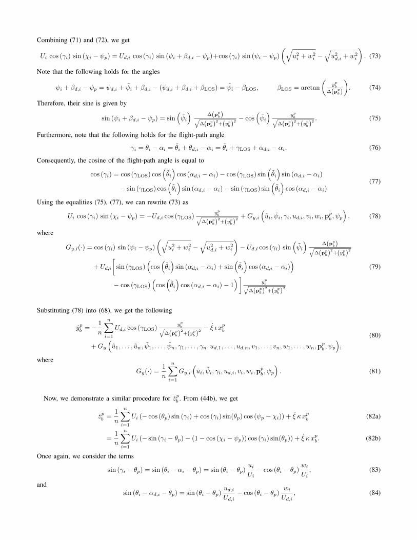
APPENDIX IIDERIVATIONS AND LEMMAS FROM SECTION V

A. Derivation of Closed-Loop Barycenter Kinematics

We begin by taking ypb from (44b).

ypb =1

n

n∑i=1

Ui cos (γi) sin (χi − ψp)− ξ ι xpb . (68)

Now, consider the term sin (χi − ψp). The course of the vessel is given by

χi = ψi + βi, βi = arcsin

(viUi

). (69)

After substituting and applying some trigonometric identities, we get

sin (χi − ψp) = sin (ψi + βi − ψp) = cos (ψi − ψp) sin (βi) + sin (ψi − ψp) cos (βi) (70a)

= cos (ψi − ψp)viUi

+ sin (ψi − ψp)√u2i + w2

i

Ui. (70b)

Consequently, the term Ui cos (γi) sin (χi − ψp) is equivalent to

Ui cos (γi) sin (χi − ψp) = cos (γi)

(cos (ψi − ψp) vi + sin (ψi − ψp)

√u2i + w2

i

). (71)

Now, consider a term sin (ψi + βd,i − ψp). Using a similar procedure, we get

sin (ψi + βd,i − ψp) = cos (ψi − ψp)viUd,i

+ sin (ψi − ψp)

√u2d,i + w2

i

Ud,i. (72)

Combining (71) and (72), we get

Ui cos (γi) sin (χi − ψp) = Ud,i cos (γi) sin (ψi + βd,i − ψp)+cos (γi) sin (ψi − ψp)(√

u2i + w2

i −√u2d,i + w2

i

). (73)

Note that the following holds for the angles

ψi + βd,i − ψp = ψd,i + ψi + βd,i − (ψd,i + βd,i + βLOS) = ψi − βLOS, βLOS = arctan

(ypb

∆(ppb)

). (74)

Therefore, their sine is given by

sin (ψi + βd,i − ψp) = sin(ψi

)∆(ppb)√

∆(ppb)2+(ypb )

2− cos

(ψi

)ypb√

∆(ppb)2+(ypb )

2. (75)

Furthermore, note that the following holds for the flight-path angle

γi = θi − αi = θi + θd,i − αi = θi + γLOS + αd,i − αi. (76)

Consequently, the cosine of the flight-path angle is equal to

cos (γi) = cos (γLOS) cos(θi

)cos (αd,i − αi)− cos (γLOS) sin

(θi

)sin (αd,i − αi)

− sin (γLOS) cos(θi

)sin (αd,i − αi)− sin (γLOS) sin

(θi

)cos (αd,i − αi)

(77)

Using the equalities (75), (77), we can rewrite (73) as

Ui cos (γi) sin (χi − ψp) = −Ud,i cos (γLOS)ypb√

∆(ppb)2+(ypb )

2+Gy,i

(ui, ψi, γi, ud,i, vi, wi,p

pb , ψp

), (78)

where

Gy,i(·) = cos (γi) sin (ψi − ψp)(√

u2i + w2

i −√u2d,i + w2

i

)− Ud,i cos (γi) sin

(ψi

)∆(ppb)√

∆(ppb)2+(ypb )

2

+ Ud,i

[sin (γLOS)

(cos(θi

)sin (αd,i − αi) + sin

(θi

)cos (αd,i − αi)

)− cos (γLOS)

(cos(θi

)cos (αd,i − αi)− 1

)]ypb√

∆(ppb)2+(ypb )

2

(79)

Substituting (78) into (68), we get the following

ypb = − 1

n

n∑i=1

Ud,i cos (γLOS)ypb√

∆(ppb)2+(ypb )

2− ξ ι xpb

+Gy

(u1, . . . , un, ψ1, . . . , ψn, γ1, . . . , γn, ud,1, . . . , ud,n, v1, . . . , vn, w1, . . . , wn,p

pb , ψp

),

(80)

where

Gy(·) =1

n

n∑i=1

Gy,i

(ui, ψi, γi, ud,i, vi, wi,p

pb , ψp

). (81)

Now, we demonstrate a similar procedure for zpb . From (44b), we get

zpb =1

n

n∑i=1

Ui (− cos (θp) sin (γi) + cos (γi) sin(θp) cos (ψp − χi)) + ξ κ xpb (82a)

=1

n

n∑i=1

Ui (− sin (γi − θp)− (1− cos (χi − ψp)) cos (γi) sin(θp)) + ξ κ xpb . (82b)

Once again, we consider the terms

sin (γi − θp) = sin (θi − αi − θp) = sin (θi − θp)uiUi− cos (θi − θp)

wiUi, (83)

andsin (θi − αd,i − θp) = sin (θi − θp)

ud,iUd,i

− cos (θi − θp)wiUd,i

, (84)

which give us the following equality

Ui sin (γi − θp) = Ud,i sin (θi − αd,i − θp) + ui sin (θi − θp) . (85)

Using a similar trick, we can write the sine as

sin (θi − αd,i − θp) = sin(θi − αLOS

)= sin

(θi

) ∆ (ppb)√∆ (ppb)

2+ (zpb )

2− cos

(θi

) (zpb )√∆ (ppb)

2+ (zpb )

2(86)

Consequently, we can rewrite (82b) as

zpb = − 1

n

n∑i=1

Ud,izpb√

∆ (ppb)2

+ (zpb )2

+ ξ κ xpb

+Gz

(u1, . . . , un, θ1, . . . , θn, γ1, . . . , γn, χ1, . . . , χn, ud,1, . . . , ud,n, v1, . . . , vn, w1, . . . , wn,p

pb , θp, ψp

),

(87)

where

Gz(·) =1

n

n∑i=1

Gz,i

(ui, θi, γi, χi, ud,i, vi, wi,p

pb , θp, ψp

), (88)

Gz,i(·) = −Ui ((1− cos (χi − ψp)) cos (γi) sin(θp))− ui sin (θi − θp)

−(

1− cos(θi

)) (zpb )√∆ (ppb)

2+ (zpb )

2− Ud,i sin

(θi

) ∆ (ppb)√∆ (ppb)

2+ (zpb )

2. (89)

B. Desired Pitch and Yaw Rate

For further calculations, we need to evaluate the desired pitch (qd,i) and yaw (rd,i) rates of the vessels. From (11d), weget the following relation between the yaw rate and the derivative of the yaw angle

qd,i = θd,i. (90)

Now, we consider the desired pitch angle from (35). Since we are investigating the path following task, we substitute γLOS

from (38) for γNSB,i. Differentiating (35) with respect to time yields

qd,i = θp(ξ) +∆ (ppb) z

pb − z

pb ∆ (ppb)

∆ (ppb)2

+ (zpb )2 +

ud,i w

u2d,i + w2

i

(91a)

= ξ κ(ξ) +

∆ (ppb)

(1n

∑nj=1 Ud,j

(zpb )√∆(ppb)

2+(zpb )

2+ ξ κ xpb +Gz(·)

)∆ (ppb)

2+ (zpb )

2

+

zpb

(−kξ

(xpb)2√

1+(xpb)2− 1

n

∑nj=1 Ud,j

(cos(γLOS,j)

2(ypb )2√

∆(ppb)2+(ypb )

2+

(zpb )2√

∆(ppb)2+(zpb )

2

)+ ypb Gy(·) + zpb Gz(·)

)∆ (ppb)

(∆ (ppb)

2+ (zpb )

2)

+ ud,iXw (ud,i + ui, uc) q + Yw (ud,i + ui, uc) (wi − wc)

u2d,i + w2

i

.

(91b)

From (11e), we get the following relation between the yaw rate and the derivative of the yaw angle

rd,i = ψd,i cos (θd,i) . (92)

Substituting the time-derivative of (36), we get

rd,i =

ψp(ξ)− ∆ (ppb) ypb − y

pb ∆ (ppb)

∆ (ppb)2

+ (ypb )2 − v√

U2d,i − v2

i

cos (θd,i) (93a)

=

ξ ι(ξ)−∆ (ppb)

(1n

∑nj=1 Ud,i

cos(γLOS)(ypb )√∆(ppb)

2+(ypb )

2− ξ ι xpb +Gy(·)

)∆ (ppb)

2+ (ypb )

2

+

ypb

(−kξ

(xpb)2√

1+(xpb)2− 1

n

∑nj=1 Ud,i

(cos(γLOS)2(ypb )

2√∆(ppb)

2+(ypb )

2+

(zpb )2√

∆(ppb)2+(zpb )

2

)+ ypb Gy(·) + zpb Gz(·)

)∆ (ppb)

(∆ (ppb)

2+ (ypb )

2)

− X (ud,i + ui, uc) r + Y (ud,i + ui, uc) (vi − vc)√u2d,i + w2

i

)cos (θd,i) .

(93b)

C. Proof of Lemma 1

In [11], it is shown that the error states (50a)–(50e) are UGES and the ocean current estimate errors (51a)–(51c) arebounded, which implies that (50a)–(51c) are forward complete. Therefore, we only need to prove that the underactuatedsway and heave dynamics (52), (53) and the barycenter dynamics (49a)–(49c) are forward complete.

First, let us consider the underactuated sway dynamics. From (52), we get

vi = Xv (ui + ud,i, uc) (ri + rd,i) + Yv (ui + ud,i, uc) (vi − vc) , (94)

where ri = ri − rd,i. Now, let us consider a Lyapunov function candidate

Vv(vi) =1

2v2i . (95)

Its derivative along the trajectories of vi is

Vv(vi) = Xv (ui + ud,i, uc) (ri + rd,i) vi + Yv (ui + ud,i, uc) (vi − vc) vi. (96)

From the boudedness of X2,i, κ(ξ), ι(ξ), ud,i, uc and vc, we can conclude that there exists some scalar βv,0 > 0 such

that∥∥∥∥[XT

2,i, κ(ξ), ι(ξ), ud,i, uc, vc

]T∥∥∥∥ ≤ β0. Moreover, from (93), we can conclude that there exist some positive functions

ar(βv,0) and br(βv,0) such that|rd,i| ≤ ar(βv,0) |vi|+ br(βv,0). (97)

Consequently, we can upper bound Vv(vi) using the following expression

Vv(vi) ≤ Xv (ui + ud,i, uc)(ri vi + ar(·)v2

i + br(·)vi)

+ Yv (ui + ud,i, uc)(v2i − vc vi

). (98)

Using Young’s inequality, we get

Vv(vi) ≤ (Xv (ui + ud,i, uc) (2 + ar(·)) + 2Yv (ui + ud,i, uc)) v2i

+Xv (ui + ud,i, uc)(r2i + br(·)2

)+ Yv (ui + ud,i, uc) v

2c

(99a)

≤ αv Vv(vi) + βv. (99b)

Using the comparison lemma, we get

Vv (vi(t)) ≤(Vv (vi(t0)) +

βvαv

)exp (αv(t− t0))− βv

αv. (100)

As Vv(vi) is defined for all t > t0, it follows that vi is also defined for all t > t0. The solutions of (52) thus fulfill thedefinition of forward completeness, as defined in [17].

Now, let us consider the underactuated heave dynamics. From (53), we get

wi = Xw (ui + ud,i, uc) (qi + qd,i) + Yw (ui + ud,i, uc) (wi − wc) +G(θi), (101)

where qi = qi − qd,i. Similar to the previous paragraph, we consider a Lyapunov function candidate

Vw(wi) =1

2w2i , (102)

whose derivative is

Vw(wi) = Xw (ui + ud,i, uc) (qi + qd,i) wi + Yw (ui + ud,i, uc) (wi − wc) wi +G(θ)wi. (103)

From the boudedness of X2,i, κ(ξ), ι(ξ), ud,i, uc and wc, we can conclude that there exists some scalar β0 > 0 such that∥∥∥∥[XT2,i, κ(ξ), ι(ξ), ud,i, uc, wc

]T∥∥∥∥ ≤ βw,0. Moreover, from (91), we can conclude that there exist some positive functions

aq(βw,0) and bq(βw,0) such that|qd,i| ≤ aq(βw,0) |wi|+ bq(βw,0). (104)

Consequently, we can upper bound Vw(wi) using the following expression

Vw(wi) ≤ Xw (ui + ud,i, uc)(qi wi + aq(·)w2

i + bq(·)wi)

+ Yw (ui + ud,i, uc)(w2i − wc wi

)+G(θi)wi. (105)


Vw(wi) ≤ (Xw (ui + ud,i, uc) (2 + aq(·)) + 2Yw (ui + ud,i, uc) + 1) w2i

+Xw (ui + ud,i, uc)(q2i + bq(·)2

)+ Yw (ui + ud,i, uc) w

2c +G(θ)2

(106a)

≤ αw Vw(wi) + βw. (106b)

Using the comparison lemma, we get

Vw (wi(t)) ≤(Vw (wi(t0)) +

βwαw

)exp (αw(t− t0))− βw

αw. (107)

Using the same arguments as in the previous paragraph, we conclude that the solutions of (53) are forward complete.Finally, let us consider the barycenter dynamics. We use a Lyapunov function candidate

Vb(ppb) =

1

2

((xpb)

2+ (ypb )

2+ (zpb )

2), (108)

whose derivative along the solutions of (49a)–(49c) is

Vb (ppb) = −kξ(xpb)

2√1 + (xpb)

2− 1

n

n∑i=1

Ud,i

cos (γLOS)2

(ypb )2√

∆ (ppb)2

+ (ypb )2

+(zpb )

2√∆ (ppb)

2+ (zpb )

2

+Gy(·) ypb +Gz(·) zpb (109a)

≤ Gy(·) ypb +Gz(·) zpb +1

2(xpb)

2. (109b)


Vb (ppb) ≤1

2

((xpb)

2+ (ypb )

2+ (zpb )

2)

+1

2

(Gy(·)2 +Gz(·)2

)= Vb (ppb) +

1

2

(Gy(·)2 +Gz(·)2

). (110)

Note that from (79) and (89), we can conclude that there exist some positive function ζy(Ud,1, . . . , Ud,n) andζz(Ud,1, . . . , Ud,n) such that

|Gy(·)| ≤ ζy(·)∥∥∥∥[u1, . . . , un, ψ1, . . . , ψn

]T∥∥∥∥ , (111)

|Gz(·)| ≤ ζz(·)∥∥∥∥[u1, . . . , un, θ1, . . . , θn

]T∥∥∥∥ . (112)

(113)

Consequently, there exists a class-K∞ function ζp(·) such that

Vp (ppb) ≤ Vp (ppb) + ζp

(v1, . . . , vn, w1, . . . , wn, u1, . . . , un, ψ1, . . . , ψn, θ1, . . . , θn

). (114)

Since all the arguments of ζp(·) are forward complete, Corollary 2.11 of [17] is satisfied and the barycenter dynamics isforward complete, thus concluding the proof of Lemma 1.

D. Proof of Lemma 2

First, we consider the sway dynamics. We take the Lyapunov function candidate Vv from (95) and simplify its derivativeby setting

[XT

1 , XT2

]= 0T.

Vv(vi) = Xv (ud,i, uc) rd,i vi + Yv (ud,i, uc) (vi − vc) vi. (115)

Next, we find an upper bound on rd,i vi. We substitute from (93), set[XT

1 , XT2

]= 0T and collect all terms that grow

linearly with vi to obtain the following expression

rd,i vi =

(vi

(1 +

∆(ppb ) xpb∆(ppb )2+(xpb)

2

)ι(ξ) 1

n

∑nj=1 Uj Ωx(γj , θp, χj , ψp) +

Yv(ud,i,uc)√u2d,i+w

2i

v2i

)cos(θd,i) + Fv(ud,i, θd,i, uc, vc, vi, wi, ri),

(116)

Fv(·) =Xv(ud,i,uc) ri−Yv(ud,i,uc) vc√

u2d,i+w

2i

vi cos(θd,i). (117)

We can bound this expression as

|rd,i vi| ≤2

n|vi| |ι(ξ)|

n∑j=1

(|uj |+ |vj |+ |wj |) + |Fv(·)| (118a)

≤ 2

n|ι(ξ)| v2

i +2

n|vi| |ι(ξ)|

∑j∈1,...,n\i

(|uj |+ |vj |+ |wj |

)+ |ui|+ |wi|

+ |Fv(·)| , (118b)

which we can substitute to (115) to obtain

Vv(vi) ≤(Xv (ud,i, uc)

2

n|ι(ξ)|+ Yv (ud,i, uc)

)v2i +

2

n|vi| |ι(ξ)|

∑j∈1,...,n\i

(|uj |+ |vj |+ |wj |

)+ |ui|+ |wi|

+ (|Fv(·)| − Yv (ud,i, uc) |vc|) |vi| .

(119)

For a sufficiently large vi, the quadratic term will dominate the linear term. Therefore, we can conclude that vi is boundedif

Xv (ud,i, uc)2

n|ι(ξ)|+ Yv (ud,i, uc) < 0. (120)

Since Yv is assumed to be always negative, the inequality is satisfied if

|ι(ξ)| < n

2

∣∣∣∣ Yv (ud,i, uc)

Xv (ud,i, uc)

∣∣∣∣ . (121)

Now, we perform a similar procedure for the heave dynamics. We take the Lyapunov function candidate Vw from (102)and simplify its derivative by setting

[XT

1 , XT2

]= 0T.

Vw(wi) = Xw (ud,i, uc) qd,i wi + Yw (ud,i, uc) (wi − wc) wi +G(θi)wi. (122)

Next, we find an upper bound on qd,i wi. We substitute from (91), set[XT

1 , XT2

]= 0T and collect all terms that grow

linearly with wi to obtain the following expression

qd,i wi = wi

(1 +


2

)κ(ξ) 1

n

∑nj=1 Uj Ωx(γj , θp, χj , ψp) + ud,i

Yw(ud,i,uc)

u2d,i+w

2iw2i + F (ud,i, uc, wc, wi, qi), (123)

F (·) = ud,iXw(ud,i,uc) ri−Yw(ud,i,uc)wc√

u2d,i+w

2i

wi. (124)


|qd,i wi| ≤2

n|κ(ξ)| w2

i +2

n|wi| |κ(ξ)|

∑j∈1,...,n\i

(|uj |+ |vj |+ |wj |

)+ |ui|+ |vi|

+ |F (·)| , (125a)


Vw(wi) ≤(Xw (ud,i, uc)

2

n|κ(ξ)|+ Yw (ud,i, uc)

)w2i +

2

n|wi| |κ(ξ)|

∑j∈1,...,n\i

(|uj |+ |vj |+ |wj |

)+ |ui|+ |wi|

+ (|F (·)| − Yw (ud,i, uc) |vc|+ |G(θi)|) |wi|+G(θi)wi.

(126)

For a sufficiently large wi, the quadratic term will dominate the linear term. Therefore, we can conclude that wi is boundedif

Xw (ud,i, uc)2

n|κ(ξ)|+ Yw (ud,i, uc) < 0. (127)

Since Yw is assumed to be always negative, the inequality is satisfied if

|κ(ξ)| < n

2

∣∣∣∣ Yw (ud,i, uc)

Xw (ud,i, uc)

∣∣∣∣ , (128)

which concludes the proof of Lemma 2.

E. Proof of Lemma 3

First, we consider the sway dynamics. We take the Lyapunov function candidate Vv from (95) and simplify its derivativeby setting X2 = 0.

Vv(vi) = Xv (ud,i, uc) rd,i vi + Yv (ud,i, uc) (vi − vc) vi. (129)

Next, we find an upper bound on rd,i vi. We substitute from (93), set X2 = 0 and collect all terms that grow linearly withvi to obtain the following expression

rd,i vi =

vi(1 +∆(ppb ) xpb

∆(ppb )2+(xpb)2

)ι(ξ) 1

n

∑nj=1 Uj Ωx(γj , θp, χj , ψp)−

ypb vi∑nj=1

cos(γLOS)ypb√∆(p

pb)

2+(ypb )

2+

zpb√

∆(ppb)

2+(zpb )

2

n∆(ppb )

(∆(ppb )2+(ypb )

2)

+

vi ∆(ppb)∑nj=1

cos(γLOS)ypb√∆(ppb)

2+(ypb )

2

n (∆(ppb)2 + (ypb )2)

+Yv(ud,i, uc)√u2d,i + w2

i

v2i

cos(θd,i) +Hv(ud,i, θd,i, uc, vc, vi, wi, ri,ppb , ξ),

(130)

Hv(·) =

(1 +∆(ppb)x

pb

∆(ppb)2 + (xpb)

2

)kξ ι(ξ)

xpb√1 + (xpb)

2−

ypb kξ xpb√

1 + (xpb)2∆(ppb)

(∆(ppb)

2 + (ypb )2)

+Xv(ud,i, uc) ri − Yv(ud,i, uc) vc√

u2d,i + w2

i

vi cos(θd,i).

(131)


|rd,i vi| ≤(

2

n|ι(ξ)|+ 3

n∆(ppb)

)|vi|

n∑j=1

(|uj |+ |vj |+ |wj |) + |Hv(·)| (132a)

≤(

2

n|ι(ξ)|+ 3

n∆(ppb)

)v2i +

(2

n|ι(ξ)|+ 3

n∆(ppb)

) ∑j∈1,...,n\i

(|uj |+ |vj |+ |wj |

)+ |ui|+ |wi|

(132b)

+ |Hv(·)| , (132c)


Vv(vi) ≤(Xv (ud,i, uc)

(2

n|ι(ξ)|+ 3

n∆(ppb)

)+ Yv (ud,i, uc)

)v2i

+

(2

n|ι(ξ)|+ 3

n∆(ppb)

) ∑j∈1,...,n\i

(|uj |+ |vj |+ |wj |

)+ |ui|+ |wi|

+ (|Hv(·)| − Yv (ud,i, uc) |vc|) |vi| .

(133)

For a sufficiently large vi, the quadratic term will dominate the linear term. Therefore, we can conclude that vi is boundedif

Xv (ud,i, uc)

(2

n|ι(ξ)|+ 3

n∆(ppb)

)+ Yv (ud,i, uc) < 0. (134)

From the definition of the lookahead distance (40), this condition is satisfied if

∆0 >3

n∣∣∣ Yv(ud,i,uc)Xv(ud,i,uc)

∣∣∣− 2 |ι(ξ)|. (135)

Now, we perform a similar procedure for the heave dynamics. We take the Lyapunov function candidate Vw from (102)

and simplify its derivative by setting X2 = 0.

Vw(wi) = Xw (ud,i, uc) qd,i wi + Yw (ud,i, uc) (wi − wc) wi +G(θi)wi. (136)

Next, we find an upper bound on qd,i wi. We substitute from (91), set X2 = 0 and collect all terms that grow linearly withwi to obtain the following expression

qd,i wi = wi

(1 +


2

)κ(ξ) 1

n

∑nj=1 Uj Ωx(γj , θp, χj , ψp)−

zpb wi∑nj=1

cos(γLOS)ypb√∆(p

pb)

2+(ypb )

2+

zpb√

∆(ppb)

2+(zpb )

2

n∆(ppb )

(∆(ppb )2+(zpb )

2)

+

wi ∆(ppb)∑nj=1

zpb√∆(ppb)

2+(zpb )

2

n (∆(ppb)2 + (zpb )2)

+ ud,iYw(ud,i, uc)

u2d,i + w2

i

w2i +Hw(ud,i, uc, vc, wi, vi, qi,p

pb , ξ),

(137)

Hw(·) =

(1 +∆(ppb)x

pb

∆(ppb)2 + (xpb)

2

)kξ κ(ξ)

xpb√1 + (xpb)

2−

ypb kξ xpb√

1 + (xpb)2∆(ppb)

(∆(ppb)

2 + (ypb )2)

+ud,iXw(ud,i, uc) ri − Yw(ud,i, uc) vc

u2d,i + w2

i

)wi.

(138)


|qd,i wi| ≤(

2

n|κ(ξ)|+ 3

n∆(ppb)

)|wi|

n∑j=1

(|uj |+ |vj |+ |wj |) + |Hw(·)| (139a)

≤(

2

n|κ(ξ)|+ 3

n∆(ppb)

)w2i +

(2

n|κ(ξ)|+ 3

n∆(ppb)

) ∑j∈1,...,n\i

(|uj |+ |vj |+ |wj |

)+ |ui|+ |wi|

+ |Hw(·)| ,

(139b)


Vw(wi) ≤(Xw (ud,i, uc)

(2

n|κ(ξ)|+ 3

n∆(ppb)

)+ Yw (ud,i, uc)

)w2i

+

(2

n|κ(ξ)|+ 3

n∆(ppb)

) ∑j∈1,...,n\i

(|uj |+ |vj |+ |wj |

)+ |ui|+ |wi|

+ (|Hw(·)| − Yw (ud,i, uc) |vc|) |wi| .

(140)

For a sufficiently large wi, the quadratic term will dominate the linear term. Therefore, we can conclude that wi is boundedif

Xw (ud,i, uc)

(2

n|κ(ξ)|+ 3

n∆(ppb)

)+ Yw (ud,i, uc) < 0. (141)

From the definition of the lookahead distance (40), this condition is satisfied if

∆0 >3

n∣∣∣ Yw(ud,i,uc)Xw(ud,i,uc)

∣∣∣− 2 |κ(ξ)|. (142)

Documents

Josef Matous Kristin Y. Pettersen Claudio Paliottaˇ