Embed Size (px)
Citation preview


Editorial Board
I
JAQM Editorial Board Editors Ion Ivan, University of Economics, Romania Claudiu Herteliu, University of Economics, Romania Gheorghe Nosca, Association for Development through Science and Education, Romania Editorial Team Cristian Amancei, University of Economics, Romania Catalin Boja, University of Economics, Romania Radu Chirvasuta, “Carol Davila” University of Medicine and Pharmacy, Romania Irina Maria Dragan, University of Economics, Romania Eugen Dumitrascu, Craiova University, Romania Matthew Elbeck, Troy University, Dothan, USA Nicu Enescu, Craiova University, Romania Bogdan Vasile Ileanu, University of Economics, Romania Miruna Mazurencu Marinescu, University of Economics, Romania Daniel Traian Pele, University of Economics, Romania Ciprian Costin Popescu, University of Economics, Romania Aura Popa, University of Economics, Romania Marius Popa, University of Economics, Romania Mihai Sacala, University of Economics, Romania Cristian Toma, University of Economics, Romania Erika Tusa, University of Economics, Romania Adrian Visoiu, University of Economics, Romania Manuscript Editor Lucian Naie, SDL Tridion

Advisory Board
II
JAQM Advisory Board Luigi D’Ambra, University “Federico II” of Naples, Italy Ioan Andone, Al. Ioan Cuza University, Romania Kim Viborg Andersen, Copenhagen Business School, Denmark Tudorel Andrei, University of Economics, Romania Gabriel Badescu, Babes-Bolyai University, Romania Catalin Balescu, National University of Arts, Romania Avner Ben-Yair, SCE - Shamoon College of Engineering, Beer-Sheva, Israel Constanta Bodea, University of Economics, Romania Ion Bolun, Academy of Economic Studies of Moldova Recep Boztemur, Middle East Technical University Ankara, Turkey Constantin Bratianu, University of Economics, Romania Irinel Burloiu, Intel Romania Ilie Costas, Academy of Economic Studies of Moldova Valentin Cristea, University Politehnica of Bucharest, Romania Marian-Pompiliu Cristescu, Lucian Blaga University, Romania Victor Croitoru, University Politehnica of Bucharest, Romania Cristian Pop Eleches, Columbia University, USA Michele Gallo, University of Naples L'Orientale, Italy Angel Garrido, National University of Distance Learning (UNED), Spain Bogdan Ghilic Micu, University of Economics, Romania Anatol Godonoaga, Academy of Economic Studies of Moldova Alexandru Isaic-Maniu, University of Economics, Romania Ion Ivan, University of Economics, Romania Radu Macovei, “Carol Davila” University of Medicine and Pharmacy, Romania Dumitru Marin, University of Economics, Romania Dumitru Matis, Babes-Bolyai University, Romania Adrian Mihalache, University Politehnica of Bucharest, Romania Constantin Mitrut, University of Economics, Romania Mihaela Muntean, Western University Timisoara, Romania Ioan Neacsu, University of Bucharest, Romania Peter Nijkamp, Free University De Boelelaan, The Nederlands Stefan Nitchi, Babes-Bolyai University, Romania Gheorghe Nosca, Association for Development through Science and Education, Romania Dumitru Oprea, Al. Ioan Cuza University, Romania Adriean Parlog, National Defense University, Bucharest, Romania Victor Valeriu Patriciu, Military Technical Academy, Romania Perran Penrose, Independent, Connected with Harvard University, USA and London University, UK Dan Petrovici, Kent University, UK Victor Ploae, Ovidius University, Romania Gabriel Popescu, University of Economics, Romania Mihai Roman, University of Economics, Romania Ion Gh. Rosca, University of Economics, Romania Gheorghe Sabau, University of Economics, Romania Radu Serban, University of Economics, Romania Satish Chand Sharma, Janta Vedic College, Baraut, India Ion Smeureanu, University of Economics, Romania Ilie Tamas, University of Economics, Romania Nicolae Tapus, University Politehnica of Bucharest, Romania Timothy Kheng Guan Teo, National Institute of Education, Singapore Daniel Teodorescu, Emory University, USA Dumitru Todoroi, Academy of Economic Studies of Moldova Nicolae Tomai, Babes-Bolyai University, Romania Victor Voicu, “Carol Davila” University of Medicine and Pharmacy, Romania Vergil Voineagu, University of Economics, Romania

Contents
III
Page Applications of Quantitative Methods to e-Commerce
Amit CHOUDHURY, Pallabi MEDHI A Simple Analysis Of Customers Impatience In Multiserver Queues 182
Ion SMEUREANU, Madalina ZURINI Spam filtering for optimization in internet promotions using bayesian analysis 199
Marilena DUMITRACHE, Stelian DUMITRA, Mircea BACIU Web services integration with distributed applications 223
Quantitative Methods Inquires
Paritosh BHATTACHARYA, Rakhi BHATTACHARJEE A Study On Weibull Distribution tfr Estimating the Parameters 234
Arie JACOBI, Shilo LIFSCHUTZ Minimization, Constraints and Composite Bezier Surfaces 242
Aura POPA Comparative Multidimensional Analysis Of Wheat Production At County Level 259
L. SAHOO, A.K. BHUNIA, D. ROY A Genetic Algorithm Based Reliability Redundancy Optimization For Interval Valued Reliabilities Of Components
270
Anass BAYAGA Multinomial Logistic Regression: Usage And Application In Risk Analysis 288
Mike C. PATTERSON, Bob HARMEL The Coin Changing Problem as a Mathematical Model 298
Gabriella MILONE A Mutivariate Strategic Perspective for the Evaluation Of Customer Satisfaction in Great Distribution
302
Enrico CIAVOLINO, Amajd D. AL-NASSER Information Theoretic Estimation Improvement To The Nonlinear Gompertz’s Model Based On Ranked Set Sampling
317
Ida CAMMINATIELLO, Michele GALLO, Tullio MENINI The Rasch Model for Evaluating Italian Student Performance 331
Software Analysis Ekram KHAN, Irshad A. ARSHAD, Taru VARSHNEY An Error Resilient and Memory Efficient Scheme For Wavelet Image Coding 350

Contents
IV
Page Marius MIHUT, Nicolae TOMAI
A Cost Model for The It Department 358 Book Review
Sabry M. ABD-EL-FATTAH Book Review on STRUCTURAL EQUATION MODELING WITH AMOS: BASIC CONCEPTS, APPLICATIONS, AND PROGRAMMING, Byrne, M. Barbara, Routledge/Taylor & Francis, New York, 2010
366

Applications of Quantitative Methods to e-Commerce
182
A SIMPLE ANALYSIS OF CUSTOMERS IMPATIENCE IN MULTISERVER QUEUES
Amit CHOUDHURY1
PhD, Department of Statistics, Gauhati University, Assam, India E-mail: [email protected]
Pallabi MEDHI2
Department of Statistics, Gauhati University, Assam, India E-mail: [email protected]
Abstract: Balking and reneging are two ways through which customer impatience finds reflection. In the analysis of stochastic reneging, it has traditionally been assumed that the distribution of patience time is state independent. However in many queuing systems, the customer is aware of its position in the system state. Hence in this paper, we assume that a customer who arrives at the queuing system gets to know the state of the system. Consequently, both balking and reneging are taken as function of system state. Both types of reneging are considered. Explicit closed form expressions of a number of performance measures are presented. A numerical example is presented to demonstrate the results derived rounds off the paper. Key words: Balking, Impatience, Queuing, Reneging. 1. Introduction These days customers are busy entities. An assumption which is often attached to the analysis of many queuing model is the customers are willing to wait as long as it is necessary to obtain service. Our fast-paced life is often inconsistent with this assumption. In queuing terminology, two characteristics through which customer’s impatience find reflection are balking and reneging. By balking, we mean the phenomenon of customers arriving for service into a non-empty queue and leaving without joining the queue. There is no balking from an empty queue. Haight (1957) has provided a rationale, which might influence a person to balk. It relates to the perception of the importance of being served which induces
Applications of Quantitative Methods to e-Commerce
183
an opinion somewhere in between urgency, so that a queue of certain length will not be joined, to indifference where a non-zero queue is also joined. A customer will be said to have reneged if after joining the system it gets impatient and leave the system without receiving service. On joining the system, it has a patience time such that in case service is unavailable within this patience time the customers renege. Reneging can be of two types- reneging till beginning of service (henceforth referred to as R_BOS) and reneging till end of service (henceforth referred to as R_EOS). A customer can renege only as long as it is in the queue and we call this as reneging of type R_BOS. It cannot renege once it begins receiving service. A common example is the barbershop. A customer can renege while he is waiting in queue. However once service get started i.e. hair cut begins, the customer cannot leave till hair cutting is over. On the other hand, if customers can renege not only while waiting in queue but also while receiving service, we call such behavior as reneging of type R_EOS. An example is processing or merchandising of perishable goods. In the analysis of reneging phenomena, one approach is to assume that each customer has a Markovian patience time, the distribution of which is state independent. However, it is our common day observation that there are systems where the customer is aware of its state in the system. For example customers queuing at the O.P.D. (out patient department) clinic of a hospital would know of their position in the queue. This invariably causes waiting customers to have higher rates of reneging in case their position in the queue is towards the end. It is not unreasonable then to expect that such customers who are positioned at a distance from the service facility have reneging rates, which are higher than reneging rates of customers who are near the service facility. In other words, we assume that customers are “state aware” and in this paper we model the reneging phenomenon in such a manner that the Markovian reneging rate is a function of the state of the customer in the system. Customers at higher states will be assumed to have higher reneging rates. The subsequent sections of this paper are structured as follows. Section 2 contains a brief review of the literature. Section 3 and section 4 contains the derivation of steady state probabilities and performance measures respectively. We perform sensitivity analysis in section 5. A numerical example is discussed in section 6. Concluding statements are presented in section 7. The appendix presented in section 8 contains some derivation. 2. Literature Survey One of the earliest work on reneging was by Barrer (1957) where he considered deterministic reneging with single server markovian arrival and service rates. Customers were selected randomly for service. In his subsequent work, Barrer (1957) also considered deterministic reneging (of both R_BOS and R_EOS type) in a multiserver scenario with FCFS discipline. The general method of solution was extended to two related queuing problems. Another early work on reneging was by Haight (1959). Ancher and Gafarian (1963) carried out an early work on markovian reneging with markovian arrival and service pattern. Ghosal (1963) considered a D/G/1 model with deterministic reneging. Gavish and Schweitzer (1977) also considered a deterministic reneging model with the additional assumption that arrivals can be labeled by their service requirement before joining the queue and arriving customers are admitted only if their waiting plus service time do not exceed some fixed amount. This assumption is met in communication systems. Kok and Tijms (1985) considered a single server queuing system where a customer becomes a lost customer when its service has not begun within a fixed time. Haghighi et al (1986) considered a markovian multiserver queuing model with balking as well as reneging. Each customer had a balking probability which was independent of the state of the system. Reneging discipline considered by them was R_BOS. Liu et al (1987) considered an infinite server markovian queuing system with reneging of type R_BOS. Customers had a choice of individual service or batch service, batch service being preferred by the customer. Brandt et al (1999) considered a S-server system with two FCFS queues, where the arrival rates at the queues and the service may depend on number of customers ‘n’ being in service or in the first queue, but the service rate was

Applications of Quantitative Methods to e-Commerce
184
assumed to be constant for n>s. Customers in the first queue were assumed impatient customers with deterministic reneging. Boots and Tijms (1999) considered an M/M/C queue in which a customer leaves the system when its service has not begun within a fixed interval after its arrival. In this paper, they have given the probabilistic proof of ‘loss probability’, which was expressed in a simple formula involving the waiting time probabilities in the standard M/M/C queue. Wang et al (1999) considered the machine repair problem in which failed machines balk with probability (1-b) and renege according to a negative exponential distribution. Bae et al. (2001) considered an M/G/1 queue with deterministic reneging. They derived the complete formula of the limiting distribution of the virtual waiting time explicitly. Choi et al. (2001) introduced a simple approach for the analysis of the M/M/C queue with a single class of customers and constant patience time by finding simple markov process. Applying this approach, they analyzed the M/M/1 queue with two classes of customer in which class 1 customer have impatience of constant duration and class 2 customers have no impatience and lower priority than class 1 customers. Performance measures of both M/M/C and M/M/1 queues were discussed. Zhang et al. (2005) considered an M/M/1/N framework with markovian reneging where they derived the steady state probabilities and formulated a cost model. Some performance measures were also discussed. A numerical example was discussed to demonstrate how the various parameters of the cost model influence the optimal service rates of the system. El- Paoumy (2008) also derived the analytical solution of Mx/M/2/N queue for batch arrival system with markovian reneging. In this paper, the steady state probabilities and some performance measures of effectiveness were derived in explicit forms. Another paper on markovian reneging was by Yechiali and Altman (2008). They derived the probability generating function of number of customers present in the system and some performance measures were discussed. Choudhury (2009) considered a single server finite buffer queuing system (M/M/1/K) assuming reneging customers. Both rules of reneging were considered and various performance measures presented under both rules of reneging. Other attempts at modeling reneging phenomenon include those by Baccelli et al (1984), Martin and Artalejo (1995), Shawky (1997), Choi, Kim and Zhu (2004), and Singh et al (2007), El- Sherbiny (2008) and El-Paoumy and Ismail (2009) etc. An early work on balking was by Haight (1957). Another work using the concepts of balking and reneging in machine interference queue has been carried out by Al-Seedy and Al-Ibraheem (2001). There have been some papers in which both balking as well as reneging were considered. Here mention may be made of the work by Haghighi et al (1986), Shawky and El-Paoumy (2000), Zhang et al (2005), El- Paoumy (2008), El- Sherbiny (2008), Shawky and El-Paoumy (2008). 3. The Model and System State Probabilities The model we deal with in this paper is the traditional M/M/k model with the restriction that customers may balk from a non-empty queue as well as may renege after they join the queue. We shall assume that the inter-arrival and service rates are λ and μ respectively. As for balking, we shall assume that each customer arriving at the system has a probability ‘1-pn-k+1’ (for kn ≥ and 0 otherwise) of balking from a non-empty queue. Customers joining the system are assumed to be of Markovian reneging type. We shall assume that on joining the system the customer is aware of its state in the system. Consequently, the reneging rate will be taken as a function of the customer’s state in the system. In particular, a customer who is at state ‘n’ will be assumed to have random patience time following exp (νn). Under R_BOS, we shall assume that
⎩⎨⎧
+=+
==
1,...knfor ck0,1,...,nfor 0
k-nνν n
and under R_EOS,

Applications of Quantitative Methods to e-Commerce
185
⎪⎩
⎪⎨
⎧
++=+
==
=
2,....k1,knfor ck1,2,...,nfor
0.nfor 0
k-nν
νν n
where c>1 is a constant. Our aim behind this formulation is to ensure that higher the current state of a customer, higher is the reneging rate. Then it is clear that the constant c has to satisfy c>1. This reneging formulation also requires that as a customer progresses in the queue from state n (n≥k+2) to (n-1), the reneging distribution would shift from exp (ν+cn-k) to (ν+cn-k-1) under R_BOS. Similarly for R_EOS. In view of the memory less property, this shifting of reneging distribution is mathematically tractable, as we shall demonstrate in the subsequent sections. To the best of our knowledge, such a formulation of reneging distribution has not been attempted in literature. Advantages of the same are however obvious. The steady state probabilities are derived by the Markov process method. We first analyze the case where customers renege only from the queue. Under R_BOS, let pn denote the probability that there are ‘n’ customers in the system. The steady state probabilities under R_BOS are given below,
10 pp μλ = , (3.1)
nnnn pnppnp μλμλ +=++ +− 11 )1( ; n=1,2,…k-1, (3.2)
{ } { } nkn
nkn
nkn
nkn pcccknkpppcccknkpp )1()1()()1()1()1( 1
11
1 −−+−++=−−++−++ −+−+
+−−
− νμλνμλ,
n = k, k+1,… (3.3) Solving recursively, we get (under R_BOS)
0})!({ pnp nnn μλ= ;n=1,2,…k (3.4)
01
2/)}1)({( })11(!{ pccckrkkpp krn
kr
kknknnn ⎥
⎦
⎤⎢⎣
⎡−−+−+= −
+=
+−− ∏ νμμλ ;n=k+1, (3.5)
where p0 is obtained from the normalizing condition ∑∞
=
=0
1n
np and is given as
1
1
2/)}1)({(
100 )}11(!{ )!(
−
+=
−+−−∞
+==⎥⎦
⎤⎢⎣
⎡−−+−++= ∏∑∑
n
kr
krkknknn
kn
k
n
nn ccckrkkpnp νμμλμλ
(3.6) The steady state probabilities satisfy the recurrence relation. Under R_BOS
{ } 1)( −= nn pnp μλ ; n=1,2,…,k
and [ ] 1})1()1({ −−− −−+−+= nknkn
n pcccknkpp νμλ ; n = k+1, k+2,…
We shall denote by KR_BOS the probability that an arriving unit has to wait on arrival (under R_BOS). Then
KR_BOS=Pr (N≥k)
∑∞
=
=kn
np . (3.7)
We may call KR_BOS as Erlang’s second (Erlang’s delay probability) formula for state dependent balking and state dependent reneging (R_BOS) in line with similar nomenclature in Medhi (2003, page 87). Under R_EOS where customers may renege from queue as well as while being served, let qn denote the probability that there are n customers in the system. Applying the Markov theory, we obtain the following set of steady state equations. 10 )( qq νμλ += , (3.8)

Applications of Quantitative Methods to e-Commerce
186
( ) nnnn qnqqnq )()1( 11 νμλνμλ ++=+++ +− ; n = 1,2,…,k-1 (3.9)
{ } { } nkn
nkn
nkn
nkn qcccnkqpqcccnkqp )1()1()1()1()1( 1
11
1 −−+++=−−++++ −+−+
+−−
− νμλνμλ; n = k, k+1, (3.10)
Solving recursively, we get (under R_EOS)
0]})(!{[ qnq nnn νμλ += ; n = 1,2,...,k (3.11)
01
2/)}1)({( )}11()(!{ qcccrkkpq krn
kr
kknknnn ⎥
⎦
⎤⎢⎣
⎡−−+++= −
+=
+−− ∏ νμνμλ ;n = k+1,…
(3.12)
where q0 is obtained from the normalizing condition ∑∞
=
=0
1n
nq and is given as
.)}11()(!{ })(!{1
1
2/)}1)({(
100
−
+=
−+−−∞
+==⎥⎦
⎤⎢⎣
⎡−−+++++= ∏∑∑
n
kr
krkknknn
kn
k
n
nn cccrkkpnq νμνμλνμλ
(3.13) The recurrence relations under R_EOS are
[ ] 1)}({ −+= nn qnq νμλ ; n = 1,2,…,k.
and { } 1)11( −−− −−++= nknkn
n qcccnkpq νμλ ; n = k+1, k+2,…
We shall denote by KR_EOS the probability that an arriving unit has to wait on arrival (under R_EOS). Then
KR_EOS=Pr (N≥k) ∑∞
=
=knnq (3.14)
which may be called Erlang’s second (Erlang’s delay probability) formula for state dependent balking and state dependent reneging (R_EOS). 4.Performance Measures An important measure is ‘L’, which denotes the mean number of customers in the system. To obtain an expression for the same, we note that L=P΄(1) where
1|)()1( ==′ ssPdsdP .
Here P(S) is the p.g.f. of the steady state probabilities. The derivation of P΄(1) is given in the appendix. From (8.1.17) and (8.2.3), the mean system size under two reneging rules are
)].1/()(})1)(,,({)},,({
))(()()},,(/{)},,({)1()[/1(
_1
0_0
_1
01
_0__
−+−−
−−−−−+−=
−
=
− ∑ccKcccpcKp
pKknpppppKpKL
BOSRk
EOSR
kBOSR
k
nn
kBOSRBOSRBOSR
νμλνμλ
νμνμνμλνμλλλν
(4.1)
)].1/()(})1)(,,({)},,({
)()},,(/{)},,({)1()[/1(
_1
0_0
_1
01
_0__
−+−−
−−−+−=
−
=
− ∑ccKcccqcKq
qKknqpqppKqKL
EOSRk
EOSR
kEOSR
k
nn
kEOSREOSREOSR
νμλνμλ
μμνμλνμλλλν
(4.2) Mean queue size can now be obtained and are given by

Applications of Quantitative Methods to e-Commerce
187
∑
∑
=
∞
+=
−−−=
−=
k
nkBOSRnBOSR
knnBOSRq
pKknpL
pknL
1__
1)_(
)(
)(
)].1/()(})1)(,,({)},,({
)()},,(/{)},,({)1()[/1(
_1
0_0
_1
01
_0_
−+−−
−−−+−=
−
=
− ∑ccKcccpcKp
pKknpppppKpK
BOSRk
EOSR
kBOSR
k
nn
kBOSRBOSR
νμλνμλ
μμνμλνμλλλν
∑=
−−−=k
nkEOSRnEOSREOSRq qKknqLL
1__)_( )(
)].1/()(})1)(,,({)},,({
))(()()},,(/{)},,({)1()[/1(
_1
0_0
_1
01
_0_
−+−−
−+−+−+−=
−
=
− ∑ccKcccqcKq
qKknqpqppKqK
EOSRk
EOSR
kEOSR
k
nn
kEOSREOSR
νμλνμλ
νμνμνμλνμλλλν
Using Little’s formula, one can calculate the average waiting time in the system and average waiting time in queue from the above mean lengths both under R_BOS and R_EOS.
Customers arrive into the system at the rate λ. However all the customers who arrive do not join the system because of balking. The effective arrival rate into the system is thus different from the overall arrival rate and is given by
)}.,,(/{)},,({)1( 01
_0_
1
0
1)_(
νμλνμλλλ
λλ
ppppKpK
ppp
kBOSRBOSR
k
n knn
knnBOSR
e
−
−
=
∞
=
+−
+−=
+= ∑ ∑
Similarly in case of R_EOS
)},,(/{)},,({)1( 01
_0_)_( νμλνμλλλλ pqppKqK kEOSREOSREOSR
e −+−= .
We have assumed that each customer has a random patience time following exp(ν). Clearly then, the reneging rate of the system would depend on the state of the system as well as the reneging rule. The average reneging rate under two reneging rules are given by
( )
( )
).()},,(/{)},,({)1(
1)}1({})1(1{11
)}1()1(){(
1_0
1_0_
01
1
01
1_BOS
k
k
nBOSRn
kBOSRBOSR
k
nn
knn
nkk
nn
k
nn
knn
knR
pKknpppppKpK
pccpcccpknpp
pcccknAvgrr
−−−+−=
⎭⎬⎫
⎩⎨⎧
−−−−+⎭⎬⎫
⎩⎨⎧
−−⎭⎬⎫
⎩⎨⎧
−′=
−−+−=
∑
∑∑∑∑
∑
=
−
=
∞
+=
−
==
∞
+=
−
μμνμλνμλλλ
νν
ν
( ) { }
( )
.)()},,(/{)},,({)1(
1)}1/({})1(1{1
)1()1(
1_0
1_0_
01
1
1
1
1_
∑
∑∑
∑∑
=
−
=
∞
+=
−
∞
+=
−
=
−−−+−=
⎭⎬⎫
⎩⎨⎧
−−−−+′=
−−++=
k
nkEOSRn
kEOSREOSR
k
nn
knn
nk
knn
kk
nnEOSR
qKknqpqppKqK
pccpcccQ
qcccnqnrrAvg
μμνμλνμλλλ
ν
νν

Applications of Quantitative Methods to e-Commerce
188
In a real life situation, customers who balk or renege represent the business lost. Customers are lost to the system in two ways, due to balking and due to reneging. Management would like to know the proportion of total customers lost in order to have an idea of total business lost. Hence the mean rate at which customers are lost (under R_BOS) is
.)(1
_
)_()_(
∑=
−−−=
+−k
nkBOSRn
BOSRBOSRe
pKknp
avgrr
μμλ
λλ
and the mean rate at which customers are lost (under R_EOS) is
.)(1
_
)_()_(
∑=
−−−=
+−k
nkEOSRn
EOSREOSRe
qKknq
avgrr
μμλ
λλ
These rates helps in the determination of proportion of customers lost which is of interest to the system manager as also an important measure of business lost. This proportion (under R_BOS) is given by
].)()[/1(1
}{
1_
)_()_(
∑=
−+−=
+−k
nkBOSRn
BOSRBOSRe
pKknp
avgrr
μμλ
λλλ
and the proportion (under R_EOS) is given by
].)()[/1(1
}{
1_
)_()_(
∑=
−+−=
+−k
nkEOSRn
EOSREOSRe
qKknq
avgrr
μμλ
λλλ
The proportion of customer completing receipt of service can now be easily determined from the above proportion. The customers who leave the system from the queue do not receive service. Consequently, only those customers who reach the service station constitute the actual load of the server. From the server’s point of view, this provides a measure of the amount of work he has to do. Let us call the rate at which customers reach the service station as λs .Then under R_BOS λs
(R_BOS)= λe (R_BOS)(1-proportion of customers lost due to reneging out of those joining the system)
( )⎭⎬⎫
⎩⎨⎧
−−= ∑∞
+=
)_(1
)_( /1 BOSRe
nkn
BOSRe pkn λνλ
( ) ( )
.)(1
_
__
∑=
−+=
−=k
nkBOSRn
BOSRBOSRe
pKknp
avgrr
μμ
λ
In case of R_EOS, one needs to recall that customers may renege even while being served and only those customers who renege from the queue will not constitute any work for the server. Thus λs
(R_EOS)= λe (R_EOS)(1-proportion of customers lost due to reneging from the queue out of those joining the system)
( )⎭⎬⎫
⎩⎨⎧
−−= ∑∞
+=
)_(1
)_( /1 EOSRe
nkn
EOSRe qkn λνλ

Applications of Quantitative Methods to e-Commerce
189
( )
( )
).1/()(})1)(,,({)},,({))(()(
)1(
1)1(
_1
0_01
_
1_)_(
01_
−−−+−+++=
−++′−=
⎟⎠
⎞⎜⎝
⎛−+
⎭⎬⎫
⎩⎨⎧
−′−=
−
=
=
==
∑
∑
∑∑
ccKcccqcKqqKknq
qKknqQ
qknqQ
EOSRk
EOSR
k
nkEOSRn
n
nkEOSRnEOSR
e
k
nn
n
nnEOSR
e
νμλνμλνμνμ
νννλ
ννλ
In order to ensure that the system is in steady state, it is necessary for the rate of
customers reaching the service station to be less than the system capacity. This translates to
.1)( <μλ ks
5. Sensitivity Analysis.
It is interesting to examine and understand how server utilization varies in response to change in system parameters. The four system parameters of interest are .,, νμλ We place below the effect of change in these system parameters on server utilization. For this purpose, we shall follow the following notational convention in the rest of this section.
pn ( νμλ ,, ) and qn ( νμλ ,, )will denote the probability that there are ‘n’ customers
in a system with parameters νμλ ,, in steady state under R_BOS and R_EOS respectively. i) If λ1> λ0, then
( )( )
0...)(!
)(!
)(...)(
1,,,,
11
101010
00
10
<+++
−+
−++
−⇒
<
++
ckkp
k
pp
k
kk
k
kk
νμμλλ
μλλ
μλλ
νμλνμλ
which is true. Hence ↑↓ λasp0 .
ii) If μ1> μ0, then ( )( )
0...)(
1)(
1!
11!
...11
1,,p,,
1100
1
1010
00
10
>+⎪⎭
⎪⎬⎫
⎪⎩
⎪⎨⎧
++−
+++⎟
⎟⎠
⎞⎜⎜⎝
⎛−++⎟⎟
⎠
⎞⎜⎜⎝
⎛−⇒
>
+
ckckkp
k
p
kk
k
kk
k
νμμνμμλ
μμλ
μμλ
νμλνμλ
which is true. Hence ↑↑ μasp0 .
iii) If ν1> ν0, then ( )( )
0.....)}1/()1(2)({(
1)}1/()1(2){(
1!
)(1
)(1
!
1,,p,,
221
200
32k
10
1k
00
10
>+⎭⎬⎫
⎩⎨⎧
−−++++−
−−+++++
⎭⎬⎫
⎩⎨⎧
++−
++⇒
>
+
+
ccckckccckckkp
ckckkp
p
k
k
νμνμνμνμμλ
νμνμμλ
νμλνμλ
which is true. Hence ↑↑ νasp0 .

Applications of Quantitative Methods to e-Commerce
190
The following can similarly be shown.
vii)
vi)
v)
0
0
0
↑↑
↑↑
↑↓
ν
μ
λ
asq
asq
asq
The managerial implications of the above results are obvious. 6. Numerical Example To illustrate the use of our results, we apply them to a queuing problem. We quote below an example from Allen (2005, page 352). ‘Customers arrive randomly (during the evening hours) at the Kitten house, the local house of questionable services, at an average rate of five per hour. Service time is exponential with a mean of 20 minutes per customer. There are two servers on duty. So many queuing theory students visits the Kitten house to collect data for this book that proprietress, Kitty Callay (also known as the Cheshire Cat) make some changes. She trains her kittens to provide more exotic but still exponentially distributed service and add three more servers, for a total of five. Her captivated, customers still complain that the queue is too long. Kitty commissions her most favoured customer Gralre K. Renga to make a study of her establishment. He is to determine the…., the number of servers she should provide so that…. the probability that an arriving customers must wait for service will not exceed 0.25.’ This is a design problem. Here λ= 5/hr and μ= 3/hr. As required by the owner of the Kitten house, we examine the minimum number of servers with different choices of k. Though not explicitly mentioned, it is necessary to assume reneging and balking. We shall assume that reneging distribution is state dependent following exp(νn) where νn is as described in section 3. Specifically, we shall assume ν=0.5/hr and considered the scenario with c=1.1. We further assume that balking rate is dependent of state and is 0.1. Various performance measures of interest computed are given in the following table. These measures were arrived at using a FORTRAN 77 program coded by the authors. Different choices of k were considered. Results relevant with regard to the requirement that the Kitten house should provide servers so that the probability that an arriving customers will find all servers busy should be <0.25 are presented in the following table. (All rates in the table as per hour rates)
Table 1: Table of Performance Measures (with λ=5, μ=3, ν=0.5, p=0.9 and c=1.1)
Number of servers Performance Measure k=2 k=3 k=4
∑∞
+= 1knnp 0.50513 0.23437 0.08755
λs (i.e. arrival rate of customers reaching service station) 3.95868 4.62644 4.88363
Effective mean arrival rate(λe) 4.58476 4.82917 4.94089 Fraction of time server is idle (p0) 0.18557 0.18879 0.18902
Average length of queue 0.37868 0.12356 0.03507 Average length of system 1.69824 1.66570 1.66295
Mean reneging rate 0.62608 0.20273 0.05726 Average balking rate 0.08305 0.03417 0.01182
Mean rate of customers lost 1.04132 0.37356 0.11637 Proportion of customers lost due to reneging, and
balking. 0.20826 0.07471 0.02327

Applications of Quantitative Methods to e-Commerce
191
From the above table it is clear that an ideal choice of k could be k=3 with
∑∞
+= 1knnp =0.23437. It may be noted here that k=4 would also satisfy the design criteria.
However, that would necessitate an additional server. Considering cost implications the idea would be to attain the design criteria with minimal number of severs. Under the assumption of balking and reneging, it appears that the proprietress need not increase the number of servers to five. Her design requirement would be met with three servers. She may therefore increase the number of servers by one. 7. Conclusion The analysis of a multiserver Markovian queuing system with state-dependent balking and state dependent reneging has been presented. Even though balking and reneging have been discussed by others, explicit expression are not available. This paper makes a contribution here. Closed form expressions of number of performance measures have been derived. To study the change in the system corresponding to change in system parameters, sensitivity analysis has also been presented. A numerical example has been discussed to demonstrate results derived. The numerical example is of indicative nature meant to illustrate the benefits of our theoretical results in a design context. 8. Appendix 8.1. Derivation of P΄(1) under R_BOS.
Let P(s) denote the probability generating function, defined by ∑∞
=
=0
)(n
nn spsP
From equation (3.2) we have
nnnn pnppnp μλμλ +=++ +− 11 )1( ; n = 1,2…k-1 .
Multiplying both sides of the equation by sn and summing over n, we get
11
1
1
1
1
1
1
1
1
11 )1(1 +
+
−
=
−
=
−
=
−
=
−− ∑∑ ∑∑ +−=− n
n
k
n
k
n
k
n
nn
nn
k
n
nn spn
ssnpspsps μμλλ (8.1.1)
From (3.3) we have
{ } { } nkn
nkn
nkn
nkn pcccknkpppcccknkpp )1()1()()1()1()1( 1
11
1 −−+−++=−−++−++ −+−+
+−−
− νμλνμλ; n = k, k+1,…
Similarly multiplying both sides of the equation by sn and summing over n
11
2
1111
})1()()1({1
})1()()({
++
∞
=
+−
∞
=
∞
=
+−+−∞
=
−−
−
∑
∑ ∑∑
−−++−+−
−−+−+=−
nn
kn
kn
kn kn
nn
knnn
kn
kn
nn
kn
spcccknks
spcccknksppspps
νμ
νμλλ
(8.1.2) Adding (8.1.1) and (8.1.2)
∑ ∑ ∑∑
∑ ∑∑ ∑−
=
∞
=
∞
=
++
+−−
=
++
+−
−
=
∞
=
+−−
=
∞
=
−−
−−−
⎥⎦
⎤⎢⎣
⎡−−++−+++−−−+−++=
⎥⎦
⎤⎢⎣
⎡+−⎥
⎦
⎤⎢⎣
⎡+⇒
1
1
11
21
1
11
1
1
1
11
1
11
11
})1()()1({)1(1})1()()({k
n kn kn
nn
knk
n
nn
nn
knnn
k
n kn
nn
knnn
k
n kn
nn
knnn
spcccknkspns
spcccknksnp
sppspsppsps
νμμνμμ
λλ

Applications of Quantitative Methods to e-Commerce
192
{ } { }
{ } { }
⎥⎥⎥⎥⎥
⎦
⎤
⎢⎢⎢⎢⎢
⎣
⎡
⎭⎬⎫
⎩⎨⎧
−−−+−+
+−+++⎭⎬⎫
⎩⎨⎧
−+⎭⎬⎫
⎩⎨⎧
−−′
−⎭⎬⎫
⎩⎨⎧
−−−
++−++−+++⎭⎬⎫
⎩⎨⎧
−+⎭⎬⎫
⎩⎨⎧
−′=
−−−⎭⎬⎫
⎩⎨⎧
−−−⎥⎦
⎤⎢⎣
⎡+++
⎭⎬⎫
⎩⎨⎧
−⇒
∑
∑∑∑
∑∑
∑∑
=
++
+−
+++
=
∞
+=
−
−
=
++
+−+++
=
∞
+=
−
++
∞
=
++
∞
=
k
n
nn
kk
kk
kk
kk
k
n
nn
kn
nnk
n
nn
kk
kkk
kkkk
kk
k
n
nn
kn
nn
kk
kk
kn
nn
kk
kk
kn
nn
spsPccspccc
spkspksspsPksnppsPs
sspsPcc
spcspcccspkspksspsPksnpsPs
sppsppsppsPsppsppspsPs
0
11
11
111
01
111
0
11
11111
01
1
11
20
11
2
)()}1({...}}{)1(1{
.........)1()()(1)()}1({
...}}{)1(1{......)1()()(
....)(...)(
ννμμ
ννμμ
λλλλ
{ } { }
{ } { }⎭⎬⎫
⎩⎨⎧
−−+⎭⎬⎫
⎩⎨⎧
−−
−⎭⎬⎫
⎩⎨⎧
−+⎭⎬⎫
⎩⎨⎧
−′−⎭⎬⎫
⎩⎨⎧
−−
⎭⎬⎫
⎩⎨⎧
−−′−⎭⎬⎫
⎩⎨⎧
−−−⎭⎬⎫
⎩⎨⎧
−−+
⎭⎬⎫
⎩⎨⎧
−−⎭⎬⎫
⎩⎨⎧
−′+⎭⎬⎫
⎩⎨⎧
−+⎭⎬⎫
⎩⎨⎧
−′=
++−+⎭⎬⎫
⎩⎨⎧
−−−⎭⎬⎫
⎩⎨⎧
−⇒
∑∑
∑∑∑
∑∑∑
∑∑∑∑
∑∑
==
−
==
−
=
∞
+=
−−
==
−
==
−
=
∞
+=
−
++
+−∞
=
∞
=
k
n
nn
k
n
nn
k
k
n
nn
k
n
nn
k
n
nn
kn
nn
k
n
nn
k
n
nn
k
k
n
nn
k
n
nn
k
n
nn
kn
nn
kk
kkk
kk
kn
nn
kn
nn
spsPscccspcsPscc
spsPsksnpsPspsP
sk
snppsPspsPcccspcsPcc
spsPksnpsPsspsPksnpsPs
sppspppssppsPspsPs
00
1
01
1
0
1
11
1
00
1
01
1
01
1
11
110
)()1()()()1(1
)()()(
)()()1()()()1(1
)()()()(
...}]{/)}1([{)()(
ννμ
μ
ννμμ
λλλ
{ } { }
{ } { }⎭⎬⎫
⎩⎨⎧
−−+⎭⎬⎫
⎩⎨⎧
−−
−⎭⎬⎫
⎩⎨⎧
−+⎭⎬⎫
⎩⎨⎧
−′−⎭⎬⎫
⎩⎨⎧
−−
⎭⎬⎫
⎩⎨⎧
−−′−⎭⎬⎫
⎩⎨⎧
−−−⎭⎬⎫
⎩⎨⎧
−−+
⎭⎬⎫
⎩⎨⎧
−−⎭⎬⎫
⎩⎨⎧
−′+⎭⎬⎫
⎩⎨⎧
−+⎭⎬⎫
⎩⎨⎧
−′=
−−+⎭⎬⎫
⎩⎨⎧
−−−⎭⎬⎫
⎩⎨⎧
−⇒
∑∑
∑∑∑
∑∑∑
∑∑∑∑
∑∑∑
==
−
==
−
=
∞
+=
−−
==
−
==
−
=
∞
+=
−
−
=
−∞
=
∞
=
k
n
nn
k
n
nn
k
k
n
nn
k
n
nn
k
n
nn
kn
nn
k
n
nn
k
n
nn
k
k
n
nn
k
n
nn
k
n
nn
kn
nn
k
n
nn
k
kn
nn
kn
nn
spsPscccspcsPscc
spsPsksnpsPspsP
sk
snppsPspsPcccspcsPcc
spsPksnpsPsspsPksnpsPs
psppsPpssppsPspsPs
00
1
01
1
0
1
11
1
00
1
01
1
01
1
1
0
10
)()1()()()1(1
)()()(
)()()1()()()1(1
)()()()(
})()(]{/)}1([{)()(
ννμ
μ
ννμμ
λλλ

Applications of Quantitative Methods to e-Commerce
193
{ } { } { } { }
{ } { } { } { }∑∑
∑ ∑∑∑
∑∑
∑∑∑ ∑
∑∑ ∑
==
−−
= =
−
=
∞
+=
−
−
==
−−
==
−∞
+= =
−
−
=
−−∞
=
∞
=
−−−+−+−
−−++′−+−++′−
−+−−−−−+
+−−′+−+−′=
−−−+++−−⇒
k
n
nn
k
n
nn
kk
k
n
k
n
nn
nn
k
n
nn
kn
nn
k
n
nn
k
n
nn
kk
k
n
nn
k
n
nn
kn
k
n
nn
nn
k
n
nn
kk
kn kn
nn
nn
spsccsPscccspscccsPscc
spsksP
sksnpsPsp
sksP
sksnppsP
spccsPcccspcccsPcc
spksPksnpssPsspksPksnpssPs
psppspsPpssppsPspsssP
00
11
1 0
1
01
10
1
00
11
01
1
1 0
1
1
0
110
)1()()1()()1(1)()1(1
)()()()(
)1()()1()()1(1)()1(1
)()()()(
)(]/)}1([{)(]/)}1([{)()(
ννννμμμμλμμ
ννννμμμμ
λλλλλλλ
sc
spc
scscP
scc
csp
scccsPsp
sksP
sksnp
spsksP
sksnppspppsPspsPsP
k
n
nn
k
k
n
nn
k
k
n
nn
nn
k
n
k
n
nn
kn
nn
knn
k
kn
nn
)1()1()(
)1(
)(
)1()()(
)(/}{/})({)())((
01
01
0
k
1n
1
1
0 01
111
−−
−+
−+
−−−++
+−+−+−=+′⇒
∑∑∑∑
∑ ∑∑∑
=−
=−
==
−
−
= =
∞
+=
−−−∞
=
ννν
μμμλλλλνμ
Now
( )
-1s 1)1()1(
)()1(
)(
)1()()(
)(/}{/)}({)(1lim)(lim
01
01
01
1
01
111
0
1
→−→
⎥⎥⎥⎥⎥⎥
⎦
⎤
⎢⎢⎢⎢⎢⎢
⎣
⎡
−−
−+
−+
−−−++
+−+−+−
+=′
∑∑∑∑
∑∑∑∑
=−
=−
==
−
=
∞
+=
−−−
=
−∞
=
ssc
spc
scscP
scc
csp
scccsPsp
sksP
sksnp
spsksP
sksnppspppsPspsP
sP k
n
nn
k
k
n
nn
k
k
n
nn
k
n
nn
k
n
nn
kn
nn
kk
n
nn
k
kn
nn
ννν
μμμλλλλ
νμ
( )
⎥⎥⎥⎥⎥⎥
⎦
⎤
⎢⎢⎢⎢⎢⎢
⎣
⎡
−−
+−
+−
−−++
−−−′+−+−
+=′
∑∑
∑∑
∑∑∑∑
=−
=−
==
==
−
=
−∞
=
)1()1()1()1(
)()1(
)1(})1({))()(/()1(1)1(
01
01
01
01
1
0
1
k
nnk
k
n
nn
k
k
nn
k
nn
k
nn
k
nn
nk
nn
k
knn
pcc
cc
cp
cccPpknp
pknpPpppPpp
P
νν
μμλλ
νμ
⎥⎥⎥⎥⎥⎥
⎦
⎤
⎢⎢⎢⎢⎢⎢
⎣
⎡
−−
+−
+−
−−++
−−−−+−
=′
∑∑
∑∑
∑∑∑∑
=−
=−
==
==
−
=
−∞
=
)1()1()1()1(
)()1(
)1())()(/()1(1)1(
01
01
01
01
1
0
1
k
nnk
k
n
nn
k
k
nn
k
nn
k
nn
k
nn
nk
nn
k
knn
pcc
cc
cp
cccPpknp
pknppppPpp
P
νν
μμλλ
ν
(8.1.3)

Applications of Quantitative Methods to e-Commerce
194
Here ∑∞
=
=0
),,()(n
nn cpcP νμλ and ∑
∞
=
=0
),,()(n
nn pppP νμλ where the symbol
),,( νμλnp is as described in section 7. We use np and ),,( νμλnp interchangeably.
However should any of the parameters νμλ ,, change, it is explicitly stated. To obtain a closed form expression for P(c) and P(p), let us for the time being, consider two another queuing systems with parameters and assumptions similar to the queuing system we are presently considering except that the arrival rate is ‘cλ’ and ‘pλ’ respectively. For these new systems, the steady state equations are same as (4.1), (4.2) and (4.3) with ‘λ’ replaced by ‘cλ’ and ‘pλ’ respectively. Denoting the steady state probabilities of these new systems by ),,( νμλcpn and ),,( νμλppn respectively, we can obtain under R_BOS
{ } ),,(!)(),,( 0 νμλμλνμλ cpnccp nnn = ; n=1,2,…,k (8.1.4)
),,()}1/1(!{)(),,( 01
2/)}1)({( νμλνμμλνμλ cpccckrkkpccp krn
kr
kknknnn ⎥
⎦
⎤⎢⎣
⎡−−+−+= −
+=
+−− ∏; n = k+1,… (8.1.5)
where
.)}11(!{)( )!()(),,(1
1
2/)}1)({(
100
−
+=
−+−−∞
+==⎥⎦
⎤⎢⎣
⎡−−+−++= ∏∑∑
n
kr
krkknknn
kn
k
n
nn ccckrkkpcnccp νμμλμλνμλ
(8.1.6)
and { } ),,(!)(),,( 0 νμλμλνμλ ppnppp nnn = ; n=1,2,…,k-1
),,()}1/1(!{)(),,( 01
2/)}1)({( νμλνμμλνμλ ppccckrkkpppp krn
kr
kknknnn ⎥
⎦
⎤⎢⎣
⎡−−+−+= −
+=
+−− ∏
n=k+1,… (8.1.7) where
.)}11(!{)( )!()(),,(1
1
2/)}1)({(
100
−
+=
−+−−∞
+==⎥⎦
⎤⎢⎣
⎡−−+−++= ∏∑∑
n
kr
krkknknn
kn
k
n
nn ccckrkkpcnppp νμμλμλνμλ
(8.1.8) Similarly, we can derive the steady state probabilities of these queuing systems under R_EOS. Let ),,;( νμλcSP denotes the probability generating function of this new queuing system so that
∑∞
=
=0
),,(),,;(n
nn spppSP νμλνμλ .
Now
[ ] 01 1
2/)}1)({(
100
01 1
2/)}1)({(
100
0
)}11(!{)(!)(})({
)}11(!{)(!)(
),,()(
pccckrkkppnppppP
pccckrkkppnppp
pppP
kn
n
kr
krkknknnk
n
nn
kn
n
kr
krkknknnk
n
nn
n
nn
∑ ∏∑
∑ ∏∑
∑
∞
+= +=
−+−−
=
∞
+= +=
−+−−
=
∞
=
⎥⎦
⎤⎢⎣
⎡−−+−++=−⇒
⎥⎦
⎤⎢⎣
⎡−−+−+++=
=
νμμλμλ
νμμλμλ
νμλ
(8.1.9)

Applications of Quantitative Methods to e-Commerce
195
Now putting S=1 in ),,;( νμλcSP we get
{ }.),,()(
9)using(8.1. ),,(c))((),,(1
(8.1.7) using ),,()}11(!{)(
!)(),,(1
),,(),,(),,;1(
00
0000
10
1
2/)}1)({(
10
10
νμλνμλνμλ
νμλνμμλ
μλνμλ
νμλνμλνμλ
cpppPpppcPcp
ppccckrkkpp
nppp
pppppP
kn
n
kr
krkknknn
k
n
nn
nn
=⇒−+=⇒
⎥⎦
⎤⎢⎣
⎡−−+−+
++=⇒
+=
∑ ∏
∑
∑
∞
+= +=
−+−−
=
∞
=
Similarly under R_EOS,
),,()( 00 νμλpqqpQ = . (8.1.10)
Using the same procedure, we can obtain, under R_BOS ),,()( 00 νμλpppcP = (8.1.11)
and under R_EOS ),,()( 00 νμλcqqcQ = . (8.1.12)
Again let ∑∞
=
=kn
nBOSR pppK ),,(),,(_ νμλνμλ
.}),,({
),,()}]11(!{)[(
00
01
)1)({(
∑
∑ ∏∞
=
∞
= +=
−+−−
=
−−+−+=
kn
nn
kn
n
kr
krkknknn
pcppp
ppccckrkkpp
νμλ
νμλνμμλ
Therefore,
∑∞
=
=kn
BOSRn
n pppKppp ),,(),,( 0_0 νμλνμλ (8.1.13)
and under R_EOS we have
∑∞
=
=kn
BOSRn
n pqpKqpq ),,(),,( 0_0 νμλνμλ . (8.1.14)
similarly under R_BOS,
∑∞
=
=kn
BOSRn
n cpcKpcp ),,(),,( 0_0 νμλνμλ (8.1.15)
and under R_EOS,
∑∞
=
=kn
BOSRn
n cqcKqcq ),,(),,( 0_0 νμλνμλ . (8.1.16)
Using these in (8.1.3), we
.)1/()()},,()1/{()},,({
))(()()},,(/{)},,({)1(1)1(
_01
_0
_1
01
_0_
⎥⎥⎥
⎦
⎤
⎢⎢⎢
⎣
⎡
−+−−
−−−−−+−=′
−
=
− ∑ccKcpcccKp
pKknpppppKpKP
BOSRk
BOSR
kBOSR
k
nn
kBOSRBOSR
νμλνμλ
νμνμνμλνμλλλ
ν
{using (3.7)} (8.1.17) where p0(cλ,μ,ν) and p0(pλ,μ,ν) are given in (8.1.6) and (8.1.8) respectively.

Applications of Quantitative Methods to e-Commerce
196
8.2. Derivation of Q΄ (1) under R_EOS From equation (3.9) we have,
( ) nnnn qnqqnq )()1( 11 νμλνμλ ++=+++ +− ; n=1,2,…,k-1.
Multiplying both sides of this equation by sn and summing over n from we get
∑∑∑∑−
=
++
−
=
−
=
−
=
−− ++−+=−
1
1
11
1
1
1
1
1
1
11 )1()(1)(
k
n
nn
nn
k
n
nk
nn
k
n
nn sqn
ssqnsqsqs νμνμλλ (8.2.1)
From equation (3.10)
{ } { } nkn
nkn
nkn
nkn qcccnkqpqcccnkqp )1()1()1()1()1( 1
11
1 −−+++=−−++++ −+−+
+−−
− νμλνμλ; n = k+1, k+2,…. Multiplying both sides of this equation by sn and summing over n from we get
11
1
2
1 1
11
1
11
})1()()1({1
})1()({
++
∞
+=
+−
∞
+=
∞
+=
+−+−∞
+=
−−
−
∑
∑ ∑∑
−−+++−
−−++=−
nn
kn
kn
kn kn
nn
knnn
kn
kn
nn
kn
sqcccnks
sqcccnksqpsqps
νμ
νμλλ
(8.2.2)
Adding (8.2.1) and (8.2.2) and proceeding in a manner similar to section (8.1), we obtain,
⎥⎥⎥
⎦
⎤
⎢⎢⎢
⎣
⎡
−+−−
−−−+−=′
−
=
− ∑)1/()()},,()1/{()},,({
)()},,(/{)},,({)1(1)1(
_01
_0
_1
01
_0_
ccKcqcccKq
qKknqpqppKqKQ
EOSRk
EOSR
kBOSR
k
nn
kEOSREOSR
νμλνμλ
μμνμλνμλλλ
ν
. {using (3.14), (8.1.14) and (8.1.15)} (8.2.3) References 1. Allen, A. Probability, Statistics and Queuing Theory with Computer Science
Application, Second Edition, Academic Press, 2005 2. Altman, E. and Yechiali, U. Infinite- Server Queues with System’s Additional Tasks
and Impatient Customers, Probability in the Engineering and Informational Sciences, Vol. 22, No. 4, 2008, pp. 477-493
3. Al-Seedly, R. O. and Al-Ibraheem, F. M. An Interarrival Hyperexponential Machine Interference with Balking, Reneging, State-dependent, Spares and an Additional Server for Longer Queues, International Journal of Mathematics and Mathematical Sciences, Vol. 27, No. 12, 2001, pp. 737-747
4. Bae, J., Kim, S. and Lee, E.Y. The virtual waiting time of the M/G/1 Queue with Impatient Customers, Queuing Systems: Theory and Applications, Vol. 38, No. 4, 2001, pp. 485-494
5. Baccelli, F., Boyer, P. and Hebuterne, G. Single Server Queues with Impatients Customers, Adv. Appl. Prob., Vol. 16, 1984, pp. 887-905
6. Barrer, D.Y. Queuing with impatient customers and ordered Service, Operations Research, Vol. 5, No. 5, 1957, pp. 650-656
7. Barrer, D.Y. Queuing with impatient customers and indifferent clerks, Operations Research, Vol. 5, No. 5, 1957, pp. 644-649
8. Boots, N.K. and Tijms, H. An M/M/c Queues with Impatient Customers, TOP, Vol. 7, No. 2, 1999, pp. 213-220

Applications of Quantitative Methods to e-Commerce
197
9. Brandt, A. and Brandt, M. On a Two-Queue Priority System with Impatience and its Application to a Call Centre, Methodology and Computing in Applied Probability, Vol. 1, No. 2, 1999, pp. 191-210
10. Choi, B. D., Kim, B. and Chung, J. M/M/1 Queue with Impatient Customers of Higher Priority, Queuing Systems, Vol. 38, No. 1, 2001, pp. 49-66
11. Choi. B. D., Kim, B. and Zhu, D. MAP/M/C Queue with Constant Impatients Times, Mathematics of Operations Research, Vol. 29, No. 2, 2004, pp. 309-325
12. Choudhury, A. A few words on Reneging in M/M/1/K queues, Contributions to Applied and Mathematical Statistics, Vol. 4, 2004, pp. 58-64
13. El-Paoumy, M. S. On Poisson Arrival Queue: MX/M/2/N with Balking, Reneging and Heterogeneous Servers, Applied Mathematical Sciences, Vol. 2, No. 24, 2008, pp. 1169-1175
14. El-Paoumy, M. S. On a Truncated Erlangian Queuing system with State-Dependent Service rate, Balking and Reneging, Applied Mathematical Sciences, Vol. 2, No. 24, 2008, pp. 1161-1167
15. El-Paoumy, M. S. and Ismail, M. M. On a truncated Erlang Queuing System with Bulk Arrivals, Balking and Reneging, Applied Mathematical Sciences, Vol. 3, No. 23, 2009, pp. 1103-1113
16. El-Sherbiny, A. A. The Non-Truncated Bulk Arrival Queue MX/M/1 with Reneging, Balking, State-Dependent and an Additional Server for Longer Queues, Applied Mathematical Sciences, Vol. 2, No. 15, 2008, pp. 747-752
17. Gavish, B. and Schweitzer, P. J. The Markovian Queue with Bounded Waiting Time. Management Science, Vol. 23, No. 12, 1977, pp. 1349-1357
18. Ghoshal, A. Queues with Finite Waiting Time, Operations Research, Vol. 11, No. 6, 1963, pp. 919-921
19. Hagighi, A. Montazer, Medhi, J. and Mohanty, S. G. On a multi server Markovian queuing system with Balking and Reneging, Computer and Operational Research. Vol. 13, No. 4, 1986, pp. 421-425
20. Haight, F. A. Queuing with Balking, Biometrika, Vol. 44, No. 3/4, 1957, pp. 360-369 21. Haight, F. A. Queuing with Reneging, Metrika, Vol. 2, No. 1, 1959, pp. 186-197 22. Ke, J. C. and Wang, K.-H. Cost analysis of the M/M/R machine repair problem with
balking, reneging and server breakdowns, The Journal of the Operational Research Society, Vol. 50, No. 3, 1999, pp. 275-282
23. Kok, A.G.D and Tijms, H. A Queuing System with Impatient customers, J. Applied Probability, Vol. 22, No. 3, 1985, pp. 688-696
24. Liu, L. and Kulkarni, V. G. Busy Period analysis for M/PH/1 queues with workload dependent Balking, Queuing Systems, Vol. 59, No. 1, 2008, pp. 37-51
25. Liu, L., Kashyap, B. R. K. and Templeton, J. G. C. The service system M/MR/∞ with impatient customers, Queuing Systems, Vol. 2, No. 4, 1987, pp. 363-372
26. Martin, M. and Artalejo, J. R. Analysis of an M/G/1 Queue with two types of Impatient units, Advances in Applied Probability, Vol. 27, No. 3, 1995, pp. 840-861
27. Medhi, J Stochastic model in Queuing Theory, Second Edition, Academic Press, 2003 28. Shawky, A. I. The single server machine interference model with balking,
reneging and an additional server for longer queues, Microelectronics Reliability. Vol. 37, 1997, pp. 355-357
29. Shawky, A. I. and El- Paoumy, M. S. The Interarrival Hyperexponential Queues: Hk/M/c/N with Balking and Reneging, Stochastics An International Journal of Probability and Stochastic Processes, Vol. 69, No. 1 and 2, 2000, pp. 67-76
30. Shawky, A. I. and El- Paoumy, M. S. The Truncated Hyper- Poisson Queues: Hk/Ma,b/c/N with Balking, Reneging and General Bulk- Service Rule, Yugoslav Journal of Operations Research, Vol. 8, No. 1, 2008, pp. 23-36
31. Singh, C. J., Kumar, B. and Jain, M. Single server interdependent queuing model with controllable arrival rates and reneging, Pakistan J. Statistics, Vol. 23, No. 2, 2007, pp. 171-178

Applications of Quantitative Methods to e-Commerce
198
32. Zhang, Y., Yue, D. and Yue, W. Analysis of an M/M/1/N queue with balking, reneging and server vacations, Paper presented in the Vth. International Symposium on OR and its Application, online source: www.aporc.org/LNOR/6/ISORA 2006F10.pdf, 2005
1 Amit Choudhury (born 1968) is a faculty member of the Dept. of Statistics, Gauhati University, India. He completed his Ph.D. from the same university and M.Stat from Indian Statistical Institute, Kolkata, India. He has about fifteen years of teaching experience in Statistics/Operations Research. His research interest is in modeling Queuing scenarios as well as in inferential aspects of Queuing theory. In addition, he has interests in statistical applications in health and education. He has more than fifteen publications in peer reviewed journals of repute in topics ranging from Statistics, Operations Research to those in Public Health, Ophthalmology and Education. He is the life member of a number of professional bodies - Operational Research Society of India, Indian Statistical Association, Indian Society for Medical Statistics, Indian Bayesian Society. Prior to joining academics, he worked for more than three years in SIDBI (Small Industries Development Bank of India). 2 Pallabi Medhi (born 1984) is a research scholar of the Dept. of Statistics, Gauhati University, India. She completed her M.Sc. from the same university in 2007. Her research interest is in modeling Queuing scenarios and in data analysis.

Applications of Quantitative Methods to e-Commerce
199
SPAM FILTERING FOR OPTIMIZATION IN INTERNET PROMOTIONS USING BAYESIAN ANALYSIS
Ion SMEUREANU1 PhD Univ. Professor Academy of Economic Studies Bucharest, Pta. Romana, no. 2-5, district 1, Romania E-mail: [email protected]
Madalina ZURINI2 Academy of Economic Studies Bucharest, Pta. Romana, no. 2-5, district 1, Romania E-mail: [email protected]
Abstract: The main characteristics of an e-business and its promoting are presented. It contains ways of promoting an e-business, examined in depth the e-mail marketing principle along with advantages and disadvantages of the implementation. E-mail marketing metrics are defined for analyzing the impact on customers. A model for optimization the promoting process via email is created for reaching the threshold of profitability for electronic business. The model implements Bayesian spam filtering and applies an internal classification, using the principles of conditioned probabilities. Key words: Bayesian spam filters; e-business; email marketing; knowledge society; metrics; Bayesian conditional probabilities
1. E-business in knowledge-based society
The knowledge society represents a new stage of human evolution, a superior
quality lifestyle that involves intensive use of IT in all spheres of human activity, with major social and economic changes. Democracy, communication, understanding and cooperation are the main characteristics of this society, which makes knowledge society to be based on the multitude resources offered by Internet access.
The business environment has changed with the evolution of Internet. A web page with contact details and the activity field have almost every small firm. As a business, for most of the times, represents keeping contact with other persons, knowledge society based on the Internet brings advantages such as: presence, communication, updated information, well served clients, interfering with new techniques of propagation such as: images, sound and video.
The term of e-business is used for the first time by IBM, being defined as a” secure, flexible and integrated access for running various businesses with the combining of processes and systems that execute the basic operations of the business with those that

Applications of Quantitative Methods to e-Commerce
200
makes possible finding information over the Internet”. E-business is more a strategy in terms of business, the main component being electronic commerce, „e-commerce”.
However, there is little information available on the Internet to help small businesses to explore the online space. Most studies simplify the structure of markets that practice e-economy by treating e-commerce companies as a generic group. The economic market encountered on the Internet can be divided into 3 structures: portal sites, market players and products and services distributors, each of which can be of 2 types: B2C, business oriented customers, or B2B, business oriented business.
Within this informatics and economic framework, the information is the one that makes the difference, and promoting an e-business is the key that opens the connections that any company needs to survive in the market.
In promoting products and services or for promotions, there are two approaches that are used in practice: mass marketing and direct marketing. Mass marketing involves media that disseminate information regarding the products through TV, radio, shops or newspapers. This type of marketing has a target group consisting in a variety of clients, there is no discrimination between them and the information is uniform transmitted. Direct marketing, on the other hand, is different from the mass one because the individual is the target group. Direct Marketing Association’s (DMA) defines this type of marketing as “communication where information are systematically used to achieve quantitative objectives and where direct contact between companies and existing customers or potential ones is realized”. From this definition it can be concluded that direct marketing classifies customers so that personalized advertisements and promotional activities can be targeted to a particular class of customers.
Over the past years, direct marketing increased in importance. Using the Internet has reduced operational costs of marketing and, even under conditions of low response from customers, it is sufficient to ensure success of the advertising campaigns.
Internet technologies offer more opportunities for online advertising. Most ads are generated by banners and sponsored content on web pages. However, in terms of online marketing, for a promotional campaign, email remains the most effective way of online promoting virtue of the precise destination, immediate response and incredibly low cost. Beyond this, it enables private communication and, properly used, helps building a long-term customers’ confidence.
2. Differences between email marketing and spam
For an effective e-marketing strategy, all actions must be linked to the business’s
objectives. The main purpose of such a strategy is to have long term benefits of a competition, based on performance. This can be achieved through research, planning, experience, analysis and news in the online industry.
Site to the principles of offline marketing that are the 4P: product, price, promotion and placement, email marketing has the main characteristics: personalization, privacy, better customers’ service, community, digital content, promotion sales, and security.
Promoting business means an expanded commercial see, public relationships, so that it brings the activity major advantages. In e-business, promotion is done with methods like:
- Domain name – as the company’s web address is a suggestive name, the more quickly persons can retain it; visit more often, one that can be easily remembered. Most areas from .com or .co.uk have been sold already, so it takes ingenuity to be able to match the name, the business field of the firm with the web page’s name. To increase the degree of familiarity, firms tend to find new names, not yet purchased, or use areas with other suffixes as .bizz.
- Search engines – Another way to encourage people to access the website of an electronic business is done through a registration on various search engines like Google, Lycos, HotBot or Yahoo. There are search engines that automatically index these websites, with links from other pages to this address. The higher the number of links, the better is the

Applications of Quantitative Methods to e-Commerce
201
position returned by the search engine, allowing people that seek information in a particular area to display the Internet pages most often used and spread. If you don’t want this to be done manually, there are specialized firms that promote web addresses using search engines.
- Sites for price comparison – Web sites such as Kelkoo can be an effective way to promote an e-business so that, for every customer directed to the business, a fee is charged for the promotion site.
- Electronic markets – Sites such as Amazon, with external businesses presented, with stocks and prices, where you can buy directly, are useful to any small or large businesses for increasing the coverage of clients. A commission is charged for each sale through these markets, commission that does not diminish the e-business profit.
- Banners, pop-ups and sponsored links – Online ads from other web addresses are a good way to promote, with a click a person is directed to the target page. A good example is Google, who wins major revenue through those sponsored links that appear in the top right of the page where search results are returned.
- Viral marketing – Represents the spread of marketing messages via email to existing customers or a target group which are then sent by those users to their acquaintance. The advantage is given by the speed and low cost.
Commercial email marketing, also called viral, is one of the most advanced communication technologies in business, changing the way vendors interact with customers. FTC, Federal Trade Commission, in [1], defines a commercial message type email, CEMM, as any email that has as main purpose the promotion of a product or service, including the content of web pages commercially organized. For many organizations, commercial email has become a medium of communications for sales.
The power of modern sales has become impressively based on email. Many sellers can’t imagine working without this tool. A research conducted by Electronic Commerce News shows that 85% of businesses use email for their communication with existing customers, 67% test the potential customers’ market, 60% use email for an internal communication and 29% of the users dispose email for online orders.
The popularity of email marketing is given by advantages such as: - lower cost than other means of communication such as direct mail
marketing; - possibility of information’s distributing to a wide audience of potential
customers using a list of emails; - dispatch time of an email is very short, order of seconds or minutes,
compared to a message sent by mail, which can last even several days; - ads can be sent to a large number of subscribers to receive communicated
via email with subjects that are part of the scope of their interests; - more than half of Internet users check their emails in a normal working day; - a precise analysis of the impact can be followed and proved to be high when
done properly; - tracking and metrics based on responses can optimize the transmission
channel of emails through a continuous process of testing, using a statistical approach of the finding results;
- email marketing is green. Email marketing offers the possibility of intercompany communication and their
clients but, there are companies that send unsolicited messages, also called spam. The priority that email marketing analyses are focused is finding the threshold beyond which existing clients treat the received advertising emails as ham, legal emails, which they wish to receive, read and respond positive in line with the target set by the companies.
The difficulty of treating emails is given by the subjectivism of the customers that receive these messages.
What is practically a spam message? To answer this question is required both definitions of this type of email.

Applications of Quantitative Methods to e-Commerce
202
Spam, objectively and lawfully seen, is an advertisement that was not requested and not given the consent to be received. The subjective definition, however, is more restrictive and, thus, more difficult to respect. Spam is all that recipient considers to be spam.
The consequences of sending messages that may be considered spam by customers who receive them have a negative effect on electronic business.
Legally, in Romania, if you send spam you can’t be punished with anything, maybe a fine if there are people with patience, time and will for claiming an email. But, technically, things get complicated.
Yahoo Mail, Gmail, Hotmail, and other such services offer the possibility of reporting those unsolicited messages, considered spam. Thus, if more people proceed in this way, future emails received by the same type as those reported will be automatically targeted spam, but not only for those users who have complained, but for all people using that mail service.
Another consequence is the possibility to block your account by the Internet provider. The blocking may occur through “black lists” which consist of spam senders and are interpreted by anti-spam filters offered default by mail servers or installed by the owners of email addresses, blocking the access of email that are considered spam.
To avoid this situation where email marketing is considered spam, it is important to take account of some recommendations such as:
- messages are sent only to those customers who have given their express consent;
- messages must be well formulated and relevant. Each mail must be unique, as each client has preferences that may differ from the others. It is important to take into account the preferences of each client as that person to handle that email as something personal;
- the address from which emails are sent must be visible, conclusive and, preferably, always the same;
- frequency of messaging is also important. Messages sent from a distance too great when the customer has an account and when he receives the first email advertising are more likely to be considered spam. Or in other circumstances, when the client is bombarded daily with messages, is not a desired approach;
- the use of specializing firm in sending messages, a company that has made a reputation with anti-spam policies formulated and implemented well. In this way, it can be avoided the blocking of these emails to different ISPs, and the rate of messages arriving in inbox, from junk mail, is higher.
3. The quality features of an e-business
Most studies conducted on the critical factors that ensure success in e-commerce
focused on limited aspects of electronic business’s operations. On the other hand, Sung, in [2], has made an identification of 16 quality
characteristics by applying a Likert scale on 5 levels for evaluation. The sample consisted of large firms in Korea, Japan and USA, who were questioned about the importance of each factor on the success of electronic business. This analysis did not include, however, SMEs (Small and Medium-sized Enterprises). Feidt, in 2002, also introduced these small businesses in research, [3], small innovative companies but with a high potential for development, suggesting that e-commerce is more a strategy then a technology. Table 1 shows, comparing the 2 analysis above, the influencing factors for small and medium companies, on the one hand, and large ones, on the other.

Applications of Quantitative Methods to e-Commerce
203
Table 1. Comparative analysis of influence factors
Commitment. Studies such as [3] and [4] have identified a commitment to business
growth and capacity of firms as a key factor for ensuring success. The growth motivation of the business can be seen by their willingness to adapt to market changes and by their strategies to constantly reinvent. They must be flexible and open to new ideas, technologies and opportunities. When necessary, businesses are prepared to seek strategic partners to provide appropriate technologies, financing, management expertise and contracts for a rapidly evolving of the business.
Content. The site serves as a central point for collecting and disseminating information related to marketing, sales and other functions of the organization, [5]. Web content must be accurate, informed, updated, understandable and related to users’ needs. In addition, online sellers should provide an adequate range of products, accurate and relevant information about the products and services held to facilitate comparison of prices with other competitors by the customers.
Convenience. Convenience factor, similar to the degree of use, refer to the development of dedicated user interfaces, and also designs and models presented on the site, [5]. E-commerce sites can implement navigation tools, such as a menu, site map, search engines, audio, video, animation and games, tools for comparing products and services to improve communication. The problem with this is finding that balance between attractive design and fast loading time because “the system response time is inversely proportional to user’s satisfaction ”, [5].
Interaction. Consumers expect high quality interaction with online merchants, mostly the customer service to be prompt and responsive, a non-stop help line, mailing lists and loyalty programs, and an effective system that realizes every step of the ordering process transparent to the users. Properly carried out these activities, it is proven to be very efficient to build confidence and customer loyalty, as it is presented in [3].
Control. The control factor evaluates the systems that e-business have integrated, defined in [5], to track and respond to questions and needs of users, the feedback and products returned, the control of the ordering process and credit risks controlling. Online sellers must audit the operations regular to measure and correct any dissatisfaction of the customers.
Community. This factor emphasizes the interaction between people and online organizations that allow participants to exchange information, such as forums, blogs. In [3],
Nr. Factors for SME (Feindt) Factors for large companies (Sung)
1 Competitive profile E-commerce strategy 2 Commitment E-commerce expertise
3 Content Variety of goods/services Plenty of information
4 Convenience Easy to use
5 Control Delivery of goods/services Payment process
6 Interaction Customer services Customer privacy
7 Community Customer relationship 8 Price sensibility Competitive pricing 9 Brand image No comparable factor 10 Partnership No comparable factor 11 Process improvement Evaluation of operations 12 Integration Low cost operations 13 Facilitations System stability, security and speed

Applications of Quantitative Methods to e-Commerce
204
it is shown that an online active community offers great opportunities for increasing the sales and productivity.
Price sensitivity. Customers expect lower prices of products and services on the Internet. A study by BizRate, [8], showed that the competitive environment forced electronic businesses to provide a reduction in transport cost, with cases in which it really is free.
Brand image. On the Internet, businesses are only one click away and customers are defined only within the language used in sites and geographical regions in which orders can be shipped concerning the economical view. Defining a brand name is essential to differentiate from other competitors in the industry. Lee and Kozar, in [7], have shown that users are willing to pay more for a company with prestige, reputation and a positive image of the brand.
Partnership. For small businesses, partnership is extremely important because of lower resources which force to work mostly closely with customers, suppliers and business partners for brand awareness, improve marketing, launching customized products. It is better to join in business community, because the position of state may attract new businesses and potential partners, being highlighted in the work [6].
Process improvement. Business process uses information technology to automate the organizational processes. This principle is easily applied to large companies, but in SMEs, financial constraints block the process.
Integration. Integrated electronic data exchange, EDI, is a system of services of quality, performance and productivity to support a large volume of business, [3]. Most small businesses don’t have the capacity for full integration only if there is support from other partners in technologically advanced.
Following the studies made by Tan, [10], a correlation matrix is resulted, table 2, having 11 influencing factors previously defined. The main diagonal is equal cu 1, state that explains that any variable is all linked, 100% correlated with itself.
We define “∩” as the correlation between two variables as:
For example, the strongest correlation is between Interaction and Content, with
value 0.628, which means that the interaction is explained with a rate of 62.8% on web page content.
Table 2. Pearson correlation matrix
The results indicated by this analysis reveals that the 11 factors listed have a
correlation between them, some more than others, correlations of which it must be taken into account in a proper marketing analysis. All parts are interconnected, not only improving a process to ensure success, it is important to find that way of comparative and correlate analysis between the main quality factors of an electronic business.

Applications of Quantitative Methods to e-Commerce
205
4. Metrics for analyzing email marketing’s impact on customers
A good method of analyzing the email marketing’s impact on customers is given by
the interpretation of metrics showing in detail the main characteristics of electronic business and the level at which they stand.
Thus, research on email marketing and spam are going to 2 lines. The first is mainly focused on reducing spam from a perspective as broad as possible, and the second includes marketing studies to determine the response rate within a promotional campaign through email. For this analysis, the definitions of metrics follow, metrics that are calculated based on the results of a campaign through email but, prior to this campaign, for a further optimization at all stages of implementation.
Sent rate (SR) is the percentage of emails that were successfully sent in the total number of emails sent.
, with . If the emails are not sent for the first time to a list of addresses, this indicator
should be included in the interval [0.9; 1]. If this indicator has values less than 0.9, this should be further examined to find the causes of this problem because such messages sent do not reach the recipients.
Opening rate (OPR) is the percentage of emails read by the customers of all emails sent successfully. This analysis can be performed on the total number of single openings and also on the multiple ones.
, with . Access rate (AR) is a very important metric, expressing how interested the customers
were of those messages sent. It is calculated as the percentage of emails accessed, representing the following of the links in the message, to the total number of emails sent successfully.
, with . Unsubscribe rate (UR) is the percentage formed by the number of client that
requested to unsubscribe from the electronic services provided through email to the total number of emails sent successfully.
, with . Forwarding rate (FR) is calculated if emails sent have a section that allows
forwarding that message to another destination. It is calculated by the number of re-sends divided by the total number of emails successfully sent.
, with . Spam rate (SPR) is defined by the percentage of spam complains to the total
number of email successfully sent.
, with .

Applications of Quantitative Methods to e-Commerce
206
Response rate (RPR) is a metric that analyzes the last step, practical purpose of email marketing, namely the interaction between customers and e-business that is completed with the purchase of products or services.
, with . Spam probability (PSPAM) represents the weight given to the entire campaign sent
emails to be classified as spam. The main cause that occurs when an email sent is treated as spam by the recipient
is explained by spam filters. In addition to the concepts defined in the preceding chapters of black lists and white lists, spam filters also have other technologies for classifying the received messages. Bayesian filtering contains an additional module which focuses on the principle of bayesian classification. This technique gives two probabilities for each word that appears in the email using the formula for conditional probabilities defined by Bayes, namely:
, where: - H is the hypothesis and D data; - is the prior probability of H, the probability that H is true before the
data D to be seen;
- means the conditional probability assigned to the data D and the
hypothesis H being satisfied; - represents the probability of data D to be realized;
- is the probability that hypothesis H is satisfied, data D being given
in reference to the earlier assumption. From this formula, it was calculated the Bayesian formula of probabilities that a
word must belong to a spam mail as:
, where:
- is the probability that the email containing the word W to be spam;
- represents the probability of occurrence of the word W in spam
emails;
- is the probability of occurrence of the word W in all emails held,
spam and ham. Complementary probability above formulated to total is described by the
formula:
, where:
- is the probability that the email containing the word W is ham;
- stands for the probability of occurrence of the word W in ham
emails.

Applications of Quantitative Methods to e-Commerce
207
As implies that .
But, . It is
enough to calculate the probability of an email containing a specific word W to be
spam, as the complementary probability, .
Having defined the formula for a word appeared in an email, to extend to the entire set of words belonging to an email, the composition al probabilities was applied, due to the independent events:
, where Wi , with , represents the n words belonging to the tested
email. The value of n can be fixed or variable, depending on the desired implementation and optimization of the final test results.
For of all promotional campaigns, we aggregate the individual probabilities of each mail sent as:
, where: - MAILj , with , represents the promotional emails and m the
number of emails sent.
5. Defining an optimization model in an email campaign To implement the principles presented in the previous chapters and of the analysis
of the indicators defined, o progressive model is realized, consisted of steps to follow to improve quality results in an ad campaign run by email communication channel.
For this, there is need of a previous collection of data with reference to existing customers database containing information on name, email, address, age, gender, occupation and categories of interest of those customers as being buyers of products and services owned and marketed by the e-business. This information will be collected from the customers when they create accounts through the web site and integrated into a well structured database.
The following is a breakdown of each step containing figure 1, along with summarizing the statistical principles for a better understanding of the concept of statistical survey.
Step1. Verification of customers’ database. As stated, the database must be constantly updated, for existing no differences between this information and the reality..
Step2. Determination of survey’s dimension. To determine the sample size is required to conduct a statistical analysis of the customers. Next, we consider the statistical population as the entire database of the customers.
Suppose we want to find the dispersion of the population when it is divided by gender. For a simple random selection of non-renewable, and a limit error chosen with a probability guarantee of results, sample size, n, is directly proportional to the dispersion of population and inversely proportional to the size of the limit error. Proposed sample size will be equal to:

Applications of Quantitative Methods to e-Commerce
208
, where: - z2 is the probability indicator that is chosen from statistical tables for a 1-α
confidence level chosen; - is the dispersion of the population with the gender classification,
variable with two states, 1 or 0, w means the weight of the population that is 0, female; - refers to the limit error chosen, expressed as a percentage. Knowing the sample size, it remains to choose those n customers from the total
population to join the next survey. Choice may be left to the program, choosing randomly, or can be generated in a different way of sorting. To simplify the process, will choose the random method.
Step3. Training the spam filter. Bayesian spam filter is a type of artificial intelligence method, one of the initiators in this field being Paul Graham in [12], [13] and [14], a method involving previously training. Training is conducted on the basis of emails collected from various sources in the company, to be able to simulate as conclusive as possible a spam filter that a customer might use it. After all emails are loaded, the filter will calculate a spam weight for each word encountered in the emails. This weight will be used in the step where PSPAM probability will be calculated.
Step4. Formulation of advertising emails. This phase includes the formulation, analysis in terms of social, psychological, economic and visual future advertising emails from the promotional campaign. It will be taken in account of previous results made, for a better understanding of the customers, their way of thinking and decision making.
Step5. PSPAM calculation. Before sending the emails, PSPAM indicator is calculated as defined in the previous chapter in order to make an earlier analysis of the sent messages. The purpose is to allow internal simulation of the messages’ interpretations by the customers.
Step6. Probability’s analysis. The metric PSPAM is compared with a threshold given, suppose the value of 0.1. If the metric’s value is below this threshold means that the emails have the probability to be considered spam less than 1%, and thus, step 7 will be preceded. Otherwise, the messages do not pass the first stage of analysis and will be redrafted and returned to step 4.
Step7. Emails’ sending to the sample set. The emails are sent to the customers selected in step 2.
Step8.Analysis of the sample’s results. Based on the results received and the feedback provided by sending the n emails, the metrics defined in chapter 4 are calculated.
Step9. Decision the extend the sample. The metrics’ results are economical analyzed and a decision is being taken whether it can continue to expand the sample throughout the population. It the results are favorable, step 10 is preceded. In the other case, the process returns to step 4, for an reassessment of the existing situation.
Step10. Sending the remaining emails. At this stage, the advertising emails are considered to be as close to that level desired by the company, having a high probability of success for the entire set of customers. The remaining emails are sent to the rest of the customers.
Step11. Final analysis. The process being finished, the last conclusions are drawn reanalyzing the defined metrics, optimizing the conclusions for a future campaign correction.

Applications of Quantitative Methods to e-Commerce
209
Fig 1. Steps of email promoting model’s implementation The principle of survey was chosen because it is more convenient for an electronic
business to test an ad campaign on a more limited range of customers than to send a message that will be interpreted negatively to a much larger population. This theory is based on the trust that given by the customers to online businesses and the level of acceptance of entering into their privacy.
6. Conclusions
The knowledge society, along with the Internet communication channel, particularly
the email, has made the promoting ways of businesses to get a different structure. Electronic businesses are seen by grown demanding of the customers who expect accurate information, concrete, rapid information to be made in a honest, convenient, interactive, to meet all the needs that a customer has.
Marketing’s new paradigm, described in [15], paradigm which is introduced by the web, makes a change from product to customer, this including a new personalized micro-level and a management of customer relationship. The problems that arise in such a

Applications of Quantitative Methods to e-Commerce
210
framework are given for how such information should be submitted, to comply with customer’s privacy, without diminishing the intensity of products and online services’ promoting
The model presented in chapter 5 optimizes the flow of information and focuses the tests made for market evaluation on a limited number of customers. The major benefit is reducing the negative effects of an advertising campaign that hasn’t the correct target group chosen, doesn’t transmit the desired and expected information to the customers and doesn’t consider the preference generally provided by the users when registering in the internal e-business system.
The best way to see the difference between email marketing and spam is in terms of the customers, those who receive these messages, because, as it was presented, spam is something subjective, in addition to legal and objective vision given by various laws, research and interpretations.
Spam is all that the recipient considers to be spam, so all we have to do left is to model the email sent to customer requirements, to personalize and optimize, to transform it from an advertising email to a personal one, applying sociological, mental, statistical, artificial intelligence and marketing theories.
References
1. Federal Trade Commission http://www.ftc.gov/ 2. Sung, T. K. E-commerce critical success factors: East vs. West, Technological
Forecasting and Social Change, Vol. 73, ISSN 0040-1625, 2006, pp. 1161-1177
3. Feindt, S., Jeffcoate, J. and Chappell, C. Identifying success factors for rapid growth in SME e-commerce, Small Business Economics Review, Vol. 19, ISSN 0921-898, 2002, pp. 51-62
4. Taylor, M. and Murphy, A. SMEs and e-business, Journal of Small Business and Enterprise Development, Vol. 11, No. 3, ISSN 1462-6004, 2004, pp. 280-289
5. Rao, S. S., Metts, G. and Monge, C. A. M. Electronic commerce development in small and medium enterprises: a stage model and its implications, Business Process Management Journal, Vol. 9, ISSN 1463-7154, 2003, pp. 11-32
6. Jeffcoate, J., Chappell, C. and Feindt, S. Best practice in SME adoption of e-commerce, Benchmarking: An International Journal, Vol. 9, No. 2, ISSN 1710-2251, 2002, pp. 122-132
7. Lee, Y. and Kozar, K. A. Investigating the effect of website quality on e-business success: an Analytic Hierarchical Approach (AHP) approach, Decision Support Systems, Vol. 42, ISSN 0167-9236, 2006, pp. 1383-1401
8. BizRate Best practices and tips for a successful holiday in 2006, e Holiday Mood Study, BizRate Research, http://www.shop.org/eholiday06/download/ eholidayreport.pdf
9. Poon, S. Business environment and internet commerce benefit: a small business perspective, European Journal of Information System, Vol. 9, ISSN 0960-085X, 2000, pp. 72-81
10. Tan, P. J. S., Sharma, R. S. and Theng, Y. L. Effective e-commerce strategies for small online retailers, International Journal of Electronic Business, Vol. 7, No. 5, ISSN 1470-6067, 2009, pp. 445-472
11. Poon, S. and Swatman, P.M.C. An exploratory study of small business internet commerce issues, Information and Management, Vol. 35, ISSN 0378-7206, 1999, pp. 9-18,
12. Worthz, J., Graham, N. and Sapte, D.W. New rules for electronic marketing – An obstacle to m-commerce?, Computer Law and Security Report, Vol. 18, No. 2, ISSN 0267-3649, 2002

Applications of Quantitative Methods to e-Commerce
211
13. Graham, P. Better Bayesian filtering, January 2003, http://paulgraham.com/better.html
14. Graham, P. A plan for Spam, August 2002, http://paulgraham.com/spam.html 15. Rust, R. T. and Espinoza, F. How technology advances influence business research
and marketing strategy, Journal Business Resource, No. 59, ISSN 1537–8020, 2006, pp. 1072-1078
1 Ion SMEUREANU has graduated the Faculty of Planning and Economic Cybernetics in 1980, as promotion leader. He holds a PhD diploma in “Economic Cybernetics” from 1992 and has a remarkable didactic activity since 1984, when he joined the staff of Bucharest Academy of Economic Studies. Currently, he is a full Professor of Economic Informatics within the Department of Economic Informatics and the dean of the Faculty of Cybernetics, Statistics and Economic Informatics from the Bucharest Academy of Economic Studies. He is the author of more than 16 books and an impressive number of articles. He was also project coordinator or member in many important research projects. He was awarded the Nicolae Georgescu-Roegen diploma, the award for the entire research activity offered by the Romanian Statistics Society in 2007 and many others. 2 Madalina ZURINI has graduated the Faculty of Cybernetics, Statistics and Economic Informatics in 2008 and she is currently conducting a master in computer science researching the implications of Bayesian classifications for optimizing spam filters. She is also engaged in a Pedagogical Program as part of the Department of Pedagogical Studies. Her fields of interest are data classification, artificial intelligence, algorithm optimisations, mathematical and econometrical analysis of factors’ influences. She wants to pursue a pedagogical career and also to give her PhD in the same area of research

Applications of Quantitative Methods to e-Commerce
212
E-BANKING IN DEVELOPING ECONOMY: EMPIRICAL EVIDENCE FROM NIGERIA
Elisha Menson AUTA PhD Candidate, Centre for Policy and Economic Research, University of Abuja, Abuja, Nigeria E-mail: [email protected]
Abstract: This paper empirically examines the impact of e-banking in Nigeria’s economy using Kaiser-Meyar-Olkin (KMO) approach and Barlett’s Test of Sphericity which support the use of factor analysis in order to extract independent variables associated with e-banking. The paper explores the major factors responsible for internet banking based on respondents’ perception on various e-banking applications. It also provides a framework of the factors which are taken to assess the e-banking perception. Due to emergence of global economy, e-business has increasingly become a necessary component of business strategy and a strong catalyst for economic development. E-banking has become popular because of its convenience and flexibility, and also transaction related benefits like speed, efficiency, accessibility, etc. The results of this study shows that e-banking serves several advantages to Nigerian banking sector. The customers (respondents) perception is that e-banking provides convenience and flexible advantages. It also provides transaction related benefits like easy transfer, speedy transaction, less cost and time saving. However, the study shows that the Nigerian customers have security, access, and no enough knowledge regarding e-banking services rendering by banking sector in Nigeria. The study suggest that critical infrastructure like power and telecommunication should be provided and with high level of stability to ensure the application of e-banking in Nigeria. Also, the relative skewed nature of banks location mostly in urban area should be addressed to ensure spread and accessibility by rural dwellers. Key words: E-banking, Developing Economy, Empirical Evidence, Nigeria
1. Introduction Financial services industry over time has opened to historic transformation that can
be termed as e-developments which is advancing rapidly in all areas of financial intermediation and financial markets such as e-finance, e-money, electronic banking (e-banking), e-brokering, e-insurance, e-exchanges, and even e-supervision. The new information technology (IT) is turning into the most important factor in the future development of banking, influencing banks’ marketing and business strategies. In recent years, the adoption of e-banking began to occur quite extensively as a channel of distribution for financial services due to rapid advances in IT and intensive competitive banking markets (Mahdi and Mehrdad, 2010; Dube, et. al., 2009). The driving forces behind the rapid transformation of banks are influential changes in the economic environment include among others innovations in information technology, innovations in financial products, liberalization and consolidation of financial markets, deregulation of financial inter-mediation. These factors make it complicated to design a bank’s strategy, which

Applications of Quantitative Methods to e-Commerce
213
process is threatened by unforeseen developments and changes in the economic environment and therefore, strategies must be flexible to adjust to these changes.
The e-banking is transforming the banking and financial industry in terms of the nature of core products /services and the way these are packaged, proposed, delivered and consumed. It is an invaluable and powerful tool driving development, supporting growth, promoting innovation and enhancing competitiveness (Gupta, 2008; Kamel, 2005). Banks and other businesses alike are turning to IT to improve business efficiency, service quality and attract new customers (Kannabiran and Narayan, 2005). Technological innovations have been identified to contribute to the distribution channels of banks and these electronic delivery channels are collectively referred to as electronic banking, (Goi, 2005). The evolution of banking technology has been driven by changes in distribution channels as evidenced by automated teller machine (ATM), Phone- banking, Tele-banking, PC-banking and most recently internet banking (Chang, 2003; Gallup Consulting, 2008).
E-banking is the term used for new age banking system. E-banking is also called online banking and it is an outgrowth of PC banking. E-banking uses the internet as the delivery channel by which to conduct banking activity, for example, transferring funds, paying bills, viewing checking and savings account balances, paying mortgages and purchasing financial instruments and certificates of deposits (Mohammed, et. a.l, 2009). It is difficult to infer whether the internet tool has been applied for convenience of bankers or for the customers’ convenience. But ultimately it contributes in increasing the efficiency of the banking operation as well providing more convenience to customers. Without even interacting with the bankers, customers transact from one corner of the country to another corner.
Electronic banking has experienced explosive growth and has transformed traditional practices in banking (Gonzalez, 2008). As per prediction of Maholtra and Singh, (2007) the e- banking is leading to a paradigm shift in marketing practices resulting in high performance in the banking industry. Delivery of service in banking can be provided efficiently only when the background operations are efficient. An efficient background operation can be conducted only when it is integrated by an electronic system. The components like data, hardware, software, network and people are the essential elements of the system. Banking customers get satisfied with the system when it provides them maximum convenience and comfort while transacting with the bank. Internet enabled electronic system facilitate the operation to fetch these result.
According to Christopher, et. al., (2006), E banking has become an important channel to sell the products and services and is perceived to be necessity in order to stay profitable in successful. There is a growing interest in understanding the users’ experience (Pyun, 2002), as e-banking is observed to be a larger concept than user satisfaction. From this perspective, assessing the user experience is essential for many technology products and services (Salehi, et. al., 2008). Customers have started perceiving the services of bank through internet as a prime attractive feature than any other prime product features of the bank. Customers have started evaluating the banks based on the convenience and comforts it provides to them.
This study aims to explore the major factors responsible for e-banking in Nigeria based on respondents’ perception on various internet applications, participants perception about e-banking and whether the user and non-user perception differs. The three critical factors of interest are convenience and flexibility, transaction related benefits, and demographic variables (gender, location, etc.)
2. Review of Literature
The concept of e-banking is a delivery channel for banking services. Banks have
used electronic channels for years to communicate and transact business with both domestic and international corporate customers. With the development of the Internet and the World Wide Web (WWW) in the latter half of the 1990s, banks are increasingly using electronic channels for receiving instructions and delivering their products and services to their

Applications of Quantitative Methods to e-Commerce
214
customers. This form of banking is generally referred to as e-banking or Internet banking, although the range of products and services provided by banks over the electronic channel vary widely in content, capability and sophistication. E-banking is defined as the automated delivery of new and traditional banking products and services directly to customers through electronic, interactive communication channels. The definition of e-banking varies amongst researches partially because electronic banking refers to several types of services through which bank customers can request information and carry out most retail banking services via computer, television or mobile phone (Daniel, 1999; Sathye, 1999). Salehi and Zhila, (2008), describes e-banking as an electronic connection between bank and customer in order to prepare, manage and control financial transactions. Electronic banking can also be defined as a variety of following platforms: (i) Internet banking (or online banking), (ii) telephone banking, (iii) TV-based banking, (iv) mobile phone banking, and e-banking (or offline banking).
E-banking includes the systems that enable financial institution customers, individuals or businesses, to access accounts, transact business, or obtain information on financial products and services through a public or private network, including the Internet or mobile phone. Customers access e-banking services using an intelligent electronic device, such as a personal computer (PC), personal digital assistant (PDA), automated teller machine (ATM), kiosk, or Touch Tone telephone. While some literature restricts the use of the term to internet banking (Daniel 1999), elsewhere the term is limited to retail banking (Aladwani 2001) or both retail and corporate banking (Simpson 2002). The common definition for e-banking, and the one used in this paper, comes from the Basel Committee Report on Banking Supervision (1998), “e-banking refers to the provision of retail and small value banking products and services through electronic channels. Such products and services can include deposit-taking, lending, account management, the provision of financial advice, electronic bill payment, and the provision of other electronic payment products and services such as electronic money”.
Karjaluoto, et. al., (2002) indicated that banks have the choice to offer their banking services through various electronic distribution channels technologies such as Internet technology, video banking technology, telephone banking technology, and WAP technology. They also indicated that Internet technology is the main electronic distribution channel in the banking industry. In other words, e-banking as an online banking that involves the provision of banking services such as accessing accounts, transferring funds between accounts, and offering an online financial service.
Wang, et. al., (2003) claims that in the 1990s e-banking was under-utilised as business organisations used it only to market their products and services. Thornton and White (2001), examined customer orientations and usage of financial distribution channels in the Australian financial industry, found that more recently most financial institutions, faced with competitive pressure after the introduction of deregulation in 1983, have rethought their strategies to take full advantage of IT. Rafiu (2007) opines that the challenge to expand and maintain banking market share has influenced many banks to invest more in making better use of the Internet. The emergence of e-banking had made many banks rethink their IT strategies in competitive markets. This findings suggest that the banks that fail to respond to the emergence of e-banking in the market are likely to lose customers and that the cost of offering e-banking services is less than the cost of keeping branch banking.
This notion was also confirmed in a study conducted by Jasimuddin (2004) examined the role of e-banking in Saudi Arabia. He indicated that the majority of Saudi banks had taken advantage of Internet technology to establish web sites but few offered e-banking services. He suggested that if the Saudi Arabian banking industry wished to be successful in the global economy it would need to integrate Internet technology into its banking strategy.
Ayo (2006) investigated the prospects of e-commerce based on ability, motivation and opportunities (AMO) model and observed that virtually all companies have online presence. The paper reported the motivation and opportunities for e-commerce as low based on lack of e-Payment infrastructure and access to information and communication technology (ICT) facilities. Also, in an empirical assessment of customer acceptance of e-

Applications of Quantitative Methods to e-Commerce
215
Commerce carried out in Germany, Buse and Tiwari (2006) observed that: the highest mobile users are top management, followed by self employed, salaried class, students and others. Government employees were found not to patronize mobile banking; the most favoured reason for carrying out mobile banking is ubiquity, next is overview of bank account, followed by immediacy; and the highest fear of customers about mobile banking is that of insecurity, next is cost, and uncomfortably.
Mahdi and Mehrdad (2010) used chi-square to determine the impact of e-banking in Iran and there findings from the view points of customers is that, e-banking cause higher advantages to Iranians. In other words, Iran banks provide services that the customers are deriving satisfaction with particular reference to the use of e-banking. In a similar study, Jayawardhena and Foley (2000) explore e-banking as a new delivery channel arguing that e-banking may help to overcome the inherent disadvantages of traditional banks; it is very clear that if e-banking conducted successfully it leads to big volume of transactions. Further, Birch and Young (1997) argue that the internet may be exploited as a new delivery channel by the financial services industry to completely reorganize the structure of banks. It means that conducting e-banking in Iran leads more usage of ATM in Iran. The authors came to conclusion that the active ATM in banking sectors will cause cash circulation decreases , the efficiency of banking sector will increase, as: a. client banking costs decreases (less cash fees to pay), b. shop keeper / service provider costs will decrease, and c. bank costs decrease (cash storage, less checking and processing costs), costumers have not enough knowledge related to e-banking in Iran. Accordingly the null hypothesis is rejected also. The authors believe that the lack of enough information on e-banking in Iran may cause less efficiency of Iranian banks. To achieving high efficiency both bankers as well as Iranian legislators should introduce e-banking services at mass level.
Chiemeke et al. (2006) conducted an empirical investigation on adoption of e-banking in Nigeria. The study identified the major inhibiting factors to Internet banking adoption in Nigeria such as, insecurity, inadequate operational facilities including telecommunications facilities and electricity supply, and made recommendations on how Nigeria banks can narrow the digital divide. Also, the report revealed that Internet banking is being offered at the basic level of interactivity with most of the banks having mainly information sites and providing little Internet transactional services.
Similarly, Agboola (2006) investigated electronic payment systems and tele-banking services in Nigeria. The findings revealed that there has been a very modest move away from cash. Payments are now being automated and absolute volumes of cash transactions have declined. The result of the study revealed that tele-banking is capable of broadening the customer relationship, retain customer’s loyalty and enable banks to gain commanding height of market share if their attendant problems such as, ineffectiveness of telecommunications services, epileptic supply of power, high cost, fear of fraudulent practices and lack of facilities necessary for their operation were taken care of.
Thus, going by the findings of most studies, we can argue that the literature on the impact of e-banking is inconclusive especially in developing economies and serve as an open ground for more research in the area of e-banking.
Framework of the factors We mention that this research survey focuses on finding the customers’ perception
on various internet application related with e-banking. Various factors which contribute to the customers’ perception such as convenience, flexible virtual banking system, reliability, time factor, real time access to information, saving transaction cost, on-line bill payments, digital signature for security, faster transfer, easy to use, user friendly, low transaction fees, any time and anywhere banking facility, access to current and historical transaction data, facility of fund transfer to third party, etc, (see Divya and Padhmanabhan, 2008) and speed, operational efficiency, better cash management, expanded financial reach (Mahrdi and Mehrdad, 2010). Some of the factors are discussed below.
1. Digital signature for security: Security is rated as the most important issue of online banking. There is a dual requirement to protect customers’ privacy and protect

Applications of Quantitative Methods to e-Commerce
216
against fraud. Digital signature is a precautionary measure to prevent malpractices and tampering the information. It is a form of enhanced authentication (Williamson, 2006).
2. Convenience way of operating banking transactions: Online banking is a highly profitable channel for financial institutions. It provides customers convenience and flexibility and can be provided at a lower cost than traditional branch banking (Beer, 2006).
3. Faster transfer: The fundamental advantage of the e-banking is the transfer of the information about the money’s worth to any place at any time with a mouse click’s distance (Dube, et. al., 2009)
4. Reliability: Kamel (2005) identified one of the very important service quality dimensions of e-banking service quality is reliability. The online banking environment has grown tremendously over the past several years and will continue to grow as financial institutions continue to strive to allow customers to complete money transfers, pay bills, and access critical information online. Authenticating customers logging onto their online banking service has become a crucial concern of financial institutions (Williamson, 2006)
5. Time factor: Liu and Arnett in their study identified time factor as one of the prime factor that in e-banking service quality feature for the customers. Saving time is an importance factor which influences the customers prefers to use e-banking. (Beer, 2006). Banks can make the information of products and services available on their site, which is, an advantageous proposition.
6. Real time access to information: The banks started e-banking with simple functions such as real time access to information about interest rates, checking account balances and computing loan eligibility. Then, the services are extended to online bill payment, transfer of funds between accounts and cash management services for corporate organizations (Mohammed, 2009).
7. Queue management: One of the important dimensions of e-banking service quality is queue management (Agboola, 2006).
8. Saving transaction cost: Improving customer service, increasing market reach and reducing costs are now basic expectations of Internet banking services. If consumers are to use new technologies, the technologies must be reasonably priced relative to alternatives. Otherwise, the acceptance of the new technology may not be viable from the standpoint of the consumer (Al-Sukhar, 2005). Internet banking model offers advantages for both banks and customers. The Internet provides the banks with the ability to deliver products and services to customers at a cost that is lower than any existing mode of delivery. Another factor that would stand in the way of consumer adoption of e-banking is the cost factor.
9. Easy to use and user friendliness: Ease of use is an important determinant for the customer preferring the internet banking (Beer, 2006). In a study conducted by Karjaluoto, et. al., (2002); reported that ease of use of innovative product or service as one of the three important characteristics for adoption from the customer’s perspective. The user friendliness of domain names as well as the navigation tools available in the web-sites is an important determinant for ease of use.
10. Any time and anywhere banking facility: Online banking users say that convenience is the most important factor, online banking lets them access their accounts from anywhere and at any time (Maholtra and Singh, 2007)
11. Access to current and historical transaction data: A customer can check balance by logging into banks website through a user name and password. In this way he can enquire balance, status of cheques, perform funds transfers, order drafts, request issue of cheque books etc (Gupta, 2008). Customers prefer to view account balances, transaction history and updates get e-statements, credit card and debit card transaction history and updates, checking the status of their credit card accounts, viewing information regarding their account, information on their fixed deposits on line.

Applications of Quantitative Methods to e-Commerce
217
3. Research Methodology Research design An exploratory research design was considered the most suitable approach in view
of the nature of the problem being investigated. A structured questionnaire adapted and modified as used by Divya and Padhmanabhan, (2009) was used as the main data-gathering instrument. The questionnaire was divided into four sections. Section A captured basic demographic information regarding the banks such as age of the bank, capital base and the number of branches nation wide. Section B captured information about the adoption and usage of e- banking services. Section C sought to determine the perceived benefits of e-banking and while section D captured information about the nature of the challenges faced in the adoption and usage of e-banking. The last two sections used a five point Likert Scale battery where the respondents were asked to indicate the extent to which they agree/disagree with various statements. The Five-Point Likert’s scale having the ratings of “strongly disagree” (1) and “strongly agree” (5) were used. Due to commercial confidentiality and sensitivity of the banking information the questionnaire was designed in a manner that did not require the respondents to reveal their names nor their banking institutions.
Data collection The study sample consisted all the 25 commercial banks in Nigeria. All the
commercial banks in Nigeria are head quartered in either Abuja (the Capital city) or Lagos, hence it was imperative to focus on these branches as they generally reflect technologies by sister branches. All the twenty-five (25) banks filled and returned the questionnaires. Data was collected over a period of three months commencing from the second week of January 2010 to the fourth week of March 2010. Statistical Package for Social Sciences (SPSS) version 10 was used as the statistical analysis tool while descriptive statistics were computed and used in the interpretation of findings.
A total of one thousand (1000) questionnaires were randomly administered to customers from diverse employment background and bankers. Seven hundred and fifty (750) were returned, which represents 75.00% of the total respondents or participants.
4. Empirical Analysis and Interpretation of Results
Factor Analysis was performed with 20 statements related with e-banking features.
The Kaiser-Meyar-Olkin (KMO) for was .754 and significant Barlett’s Test of Sphericity supported the use of factor analysis in order to extract independent variables associated with e-banking. The degree of common variance among the twenty variables is “mediocre” which reflects if a factor analysis is conducted, the factors extracted will account for fare amount of variance but not a substantial amount.
An exploratory principal component factor analysis was done using SPSS 16.0. Varimax rotation was used to identify the underlying factors for e-banking features. Items with eigen values greater than one were extracted and all factor loading greater than 0.5 were retained. Twenty items yielded 6 factors explaining 88.05 percent of variance as shown in table 1.

Applications of Quantitative Methods to e-Commerce
218
Table 1. Rotated Component Matrix
Factors Items Factor Loadings
Variance Explained
Reliability (Cronbach’s Alpha)
1. Time factor
15.345 .812
2. Security
17.560 .765
3. Queue management
12.565 .764
4. User friendly
14.420 .910
5. Fund transfer
15.2085 .650
6. Accessibility
13.075 .673
88.05 The variables above are considered as fundamental consideration associated with
e-banking. General perception about e-banking was gauged by 20 items. Out of which six items were related with convenience and flexibility and 9 items were related with transaction related benefits, and 5 items were related to access or location. All items were measured on a scale of 1to 5. From the questionnaire convenience and flexibility related items clubbed together and average score taken to gauge the respondents’ perception about convenience factor. Out of total respondents 84 % respondents felt that e-banking is very convenient and flexible. And same percentage that is, 84% from total users agrees or strongly agrees that e-banking is convenient. They felt that it gives benefits like no queuing in bank and one can do anytime and anywhere banking. Approx 79% of total respondent agreed that internet banking has transaction related benefits. These benefits include efficient and speedy transfer of funds with lower transaction cost. And, with e-banking can check transaction details regularly without any hassle. This result found support in Mahrdi and Mehrdad, (2010); Divya and Padhmanabhan, (2009) but contrary to Buse and Tiwani (2006).
Generally, most banks in Nigeria are located within the city or urban centres where infrastructure is available. Therefore, examining e-banking with respect to location became insignificant since banking services are rural-biased. Thus, the study has location challenge by rural and peri-urban dwellers in Nigeria who are compelled to move to the city to access banking services.

Applications of Quantitative Methods to e-Commerce
219
Table 2: Testing of factors which contribute to the customers’ perception
Factors Items Cronbach Alpha
Convenience and flexibility • -A convenient way of operating banking transactions - A - Avery flexible virtual banking system • - Save time as compared to conventional banking • - No queuing in bank branches • - Easy to use/ user friendly • - any time /any where banking facility •
0.840
Transaction related benefits -saves a lot of transaction cost -transaction is efficient - it has lower transaction fees - it allows speedy transfer - it allows easy access to transaction data both recent and historical -it can check transaction details and statement regularly - it gives facility to fund transfer to third party - Speed - Better cash management
0.793
Source: Variables (factors and items) source from Divya and Padhmanabhan (2008) The bio-data of participants is summarized in Appendix 1: The bio-data in appendix 1 shows that out of 750 participants 411 (54.80%) are
male and 339 are female. It means that the majority of participants are male. Majority of the respondents were between the ages 31 to 40 years, which represent 51.90% followed by ages 41 to 50 years with 29.60%. Relating to job position, most of the respondents were from the private sector 37.60% followed by public sector 32.14%. While 43 (5.73%) were clerks and others (teacher, student and housewife) 55(7.33%).
Regarding to educational background, out of 750 respondents 326(43.47%) had bachelor degree or higher national diploma (HND) followed by Diploma and national certificate of education (NCE) 120(16.00). Master degree had 195(26.00) participants. The least number of participants had PhD degree and Professor 109(14.53%). The location of the participants shows that most of the respondents resides in urban area 509(67.87), peri-urban 204(27.20), and rural area has the least with 37(4.93). The ratio of participants with respect to customer and bankers shows 448(59.73%) and 302(40.27%) respectively.
5. Conclusion
The banking industry play a significant role in supporting economic development
through efficient financial services (Dube, et. al., 2009; Salehi and Azary, 2008). Nigerian banks have embraced innovative banking technologies and e-banking services in recent years. Almost all banks have invested in expanding and improving the Information Technology systems and a number of new e-banking services have been developed. All the 25 commercial banks operating in Nigeria have declared e-business as one of the core strategies for the future development. At the same time, e-banking acceptance depends probably on bank service quality, customer preferences and satisfaction.
The analysis done with the help of statistical tools clearly indicate the factors responsible for e-banking. Factor analysis results indicate that security, user friendly, queue management, accessibility, time factor and fund transfer are major factors. Out of total respondents’ about 88% agreed that e-banking is convenient and flexible way of banking and it also has various transaction related benefits. Thus, Providing e-banking is increasingly

Applications of Quantitative Methods to e-Commerce
220
becoming a matter of need to banks to continue to compete in a globalized work and gain market competitive advantage. References
1. Aarma, A. and Vensel, V. Banks’ Retail Customer Satisfaction and Development of
Bank-Customer relationships., in Vensel, V. and Wihlborg, C. (eds). Estonia on the Threshold of the European Union: Financial Sector and Enterprise Restructuring in the Changing Economic Environment, Tallinn: Tallinn Technical University, 2001, pp. 85–106
2. Agboola, A. A. Electronic Payment Systems and Tele-banking Services in Nigeria, Journal of Internet Banking and Commerce, Vol. 11, No. 3, December 2006, online source: http://www.arraydev.com/commerce/jibc/
3. Ahasanul, H. Issues of E-banking Transaction: An Empirical Investigation on Malaysian Customers Perception, Journal of applied Sciences, 2009, retrieved from www.ebsco.com on 20 April 2010
4. Aladwani, A. Online Banking: A Field Study of Drivers, Development Challenges, and Expectations, International Journal of Information Management, 21, 2001, pp. 213–225
5. Al-Sukkar, H. Toward a Model for the Acceptance of Internet Banking in Developing Countries, Information Technology for Development, Vol. 11, No. 4, 2005, pp.381-398
6. Awamleh, R. and Fernandez Internet Banking: An Empirical Investigation into the Extent of Adoption by Banks and the Determinants of Customer Satisfaction in the United Arab Emirates, Journal of Internet Banking and Commerce, Vol. 13, No 4, 2005
7. Ayo, Charles K. The Prospects of e-Commerce Implementation in Nigeria, Journal of Internet Banking and Commerce, Vol. 11, No.3, December 2006, online source:http://www.arraydev.com/commerce/jibc/
8. Basel Committee Report on Banking Supervision Risk management for electronic banking and electronic money activities, Switzerland: Bank of International Settlements, 1998
9. Beer, S. Customers Preference on Internet Banking, 2006, Survey (Retrieved from http://www.itwire.com/content/view/4570/53 on 20 March 2010
10. Birch, D. and Young, M. Financial Services and the Internet: What Does the Cyberspace Mean for the Financial Services Industry?, Internet Research: Electronic Networking Applications and Policy, Vol.7, No. 2, 1997, pp. 120-128
11. Buse, S. and Tiwari, R. Mobile Banking Stages a Remarkable Come Back, Press Release, 2006, Retrieved 23 April, 2010, online source: http://www1.uni-hamburg.de/m-commerce/banking/index_e.html
12. Chang, Y. T. Dynamics of Banking Technology Adoption: An Application to Internet Banking, Department of Economics, Workshop Presentation, University of Warwick, Coventry, UK, 2003
13. Chiemeke, S. C., Evwiekpaefe, A. and Chete, F. The Adoption of Internet Banking in Nigeria: An Empirical Investigation, Journal of Internet Banking and Commerce, vol. 11, No.3, December 2006
14. Christopher, G. C., Mike, L. Visit and Amy, W. A Logit Analysis of Electronic Banking in New Zealand, International Journal of Bank Market, 24, 2006, pp. 360-383
15. Daniel, E. Provision of Electronic Banking in the UK and the Republic of Ireland, International Journal of Bank Marketing, Vol. 17, No. 2, 1999, pp. 72–82
16. Divya, S. and Padhmanabhan, V. A Study on Customer Perception Towards Internet Banking: Identifying Major Contributing Factors”, The Journal of Nepalese Business Studies, Vol. V No. 1, December 2008, pp 101-111

Applications of Quantitative Methods to e-Commerce
221
17. Dube, T., Chitura, T., Chitura, T. and Langton, R. Adoption and Use of Internet Banking in Zimbabwe: An Exploratory Study, Journal of Internet Banking and Commerce, April 2009, Vol. 14, 2009, No.1
18. Gallup Consulting Using Technology to Engage Retail Banking Customer, 2008, online source: http://www.adope.com/engagement/
19. Goi, C. L. E-banking in Malaysia: Opportunities and Challenges, Journal of Internet Banking and Commerce Vol. 10, No. 3, December 2005
20. Gonzalez, M. E. An Alternative Approach in Service Quality: An E-Banking Case Study, Quality Manage, 15, 2008, pp. 41-48
21. Gupta, P. K. Internet Banking in India: Consumer Concern and Bank Strategies, Global Journal of Business Research, Vol. 2, No. 1, 2008, pp. 43-51
22. Guru, C. E-banking in Transition Economies: The Case of Romania, Journal of Financial Services Marketing, Vol. 6, No. 4, 2002, pp. 362–379
23. Jasimuddin, S. Saudi Arabia Banks, 2004, Retrieved 25 April, 2010, online source: www.arraydev.com/commerce/jibc/0103-02.htm
24. Jayawardhena, C. and Foley, P. Changes in the Banking Sector: The Case of Internet Banking in the UK, Internet Research: Electronic Networking Applications and Policy, Nol.10, No.1, 2000, pp. 19-30
25. Joseph, M., McClure, C. and Joseph, B. Service Quality in Banking Sector: The Impact of Technology on Service Delivery, International Journal of Bank Marketing, 17(4), 1999, pp. 182–191
26. Kamel, S. The Use of Information Technology to Transform the Banking Sector in Developing Nations, Information Technology for Development, Vol.11, No. 4, 2005, pp. 305-312
27. Kannabira G. and Narayan, H. Deploying internet Banking and e-Commerce: Case Study of a Private Sector Bank in India, Information Technology for Development, Vol. 11, No. 4, 2005, pp. 363-379
28. Karjaluoto, Heikki; Mattila, Minna; Pento, Tapio Electronic Banking in Finland: Consumer Beliefs and Reactions to a New Delivery Channel, Journal of Financial Services Marketing, Vol. 6, No. 4, 2002, pp. 346–361
29. Mahdi, S. and Mehrdad, A. E-Banking in Emerging Economy: Empirical Evidence of Iran, International Journal of Economics and Finance, Vol. 2, No. 1, February 2010, pp. 201-209
30. Maholtra, P. and Singh, B. Determinants of Internet Banking Adoption by Banks in India, Emerald Internet Research Vol. 17, No. 3, 2007, pp. 323-339
31. Mohammed, S. K.; Siba Sankar Mahapatra and Sreekumar Service Quality Evaluation in Internet Banking: An Empirical Study in India, International Journal of Indian Culture and Business Management, Vol. 2, No. 1, 2009
32. Mayer, C. Financial Systems, Corporate Finance, and Economic Development, In: Hubbard, R.G. (Eds.), Asymmetric Information, Corporate Finance and Investment. University of Chicago Press, Chicago, 1990, pp. 307–332
33. Mols, N. The Behavioral Consequences of PC banking, International Journal of Bank Marketing, Vol. 16, No. 5, 1998, pp. 195–201
34. Pohjola, M. The New Economy: Facts, Impacts and Policies, Information Economics and Policy, 14, 2002, pp. 133–144
35. Pyun, Chong Soo; L. Scruggs, N. Nam Internet Banking in the US, Japan and Europe, Multinational Business Review, Fall 2002, pp. 73– 81
36. Rafiu, Oyesola Salawu The Emergence of Internet Banking in Nigeria: An Appraisal, Information Technology Journal, Vol. 6, No. 4, 2007, pp. 490-496
37. Salehi, Mahdi and Zhila, Azary. Fraud Detection and Audit Expectation Gap: Empirical Evidence from Iranian Bankers, International Journal of Business and Management, Vol. 3, No. 10, 2008, pp. 65-77
38. Salehi, Mahdi; Ali, Mansouri and Zhila Azary. Islamic Banking Practice and Satisfaction: Empirical Evidence from Iran, ACRM Journal of Business and Management Research, Vol. 3, No.2, 2008, pp. 35-41

Applications of Quantitative Methods to e-Commerce
222
39. Sathye, Milind. Adoption of Internet Banking by Australian Consumers: An Empirical Investigation, International Journal of Bank Marketing, Vol. 17, No. 7, 1999, pp. 324–334
40. Simpson, J. The Impact of the Internet in Banking: Observations and Evidence from Developed and Emerging Markets, Telematics and Informatics, Vol. 19. No. 4, 2002, pp. 315–330.
41. Suganthi, Balachandher, and Balachandran Internet Banking Patronage: An Empirical Investigation of Malaysia, Journal of Internet Banking and Commerce, Vol. 6, No. 1, 2001, online source: http://www.arraydev.com/commerce/JIBC/0103_01.htm March 2010
42. Thornton, J. and L. White Customer Orientation and Usage of Financial Distribution Channels, Journal of Services Marketing, Vol. 15, No. 3, 2001 pp. 168-185
43. Wang, Y. S., Y. M. Wang, H. H. Lin, and T. I. Tang Determinants of User Acceptance of Internet Banking: an Empirical Study, International Journal of Service Industry Management, Vol. 14 No. 5, 2003, pp. 501-19
44. Williamson, Gregory D. Enhanced Authentication In Online Banking, Journal of Economic Crime Management, Vol. 4, Issue 2, 2006
Appendix 1: Bio-data of participants or respondents
Variable Category Frequency Percentage Male 411 54.80 Gender
Female 339 45.20 20 – 30 54 7.20 31 - 40 389 51.90 41 – 50 222 29.60
Age
51 & above 85 11.30 Clerk 43 3.73
Private sector 282 37.60 Public sector 241 32.14
Public servant 129 17.20
Job Position
Others 55 7.33 Diploma/NCE 120 16.00 Degree/HND 326 43.47
Master 195 26.00
Education
PhD/Professor 109 14.53 Rural 37 4.93
Peri-rural 204 27.20 Location
Urban 509 67.87 Customer 448 59.73 Participants
Banker 302 40.27 Source: Field Survey 2010 (January – March)

Applications of Quantitative Methods to e-Commerce
223
WEB SERVICES INTEGRATION WITH DISTRIBUTED
APPLICATIONS
Marilena DUMITRACHE
PhD Student, Faculty of Cybernetics Statistics and Economic Informatics, Academy of Economic Studies, Bucharest, Romania E-mail: [email protected]
Stelian DUMITRA
PhD Student, Faculty of Cybernetics Statistics and Economic Informatics, Academy of Economic Studies, Bucharest, Romania
E-mail: [email protected]
Mircea BACIU
PhD Student, Faculty of Cybernetics Statistics and Economic Informatics, Academy of Economic Studies, Bucharest, Romania E-mail: [email protected]
Abstract: A Web service is a distributed application component. Web services distributed computing model allows application-to-application communication. There is nothing fundamentally new about the basic concept and the related technologies. The innovative thing about this is the reach of Web services and its ubiquitous support by literally all major vendors. Most likely, heterogeneity will at the end no longer be an obstruction for distributed applications. This paper describes the concept of service-oriented architecture (SOA) in conjunction with the Web services technology and covers the core Web services specifications which form a powerful and robust foundation for building distributed systems. It is presented a case study regarding the integration of the Web services with the SAP system for handling interoperability issues. The conclusions and the future proposed developments are presented in the end of the paper. Key words: distributed application; web service; sap; protocols; security

Applications of Quantitative Methods to e-Commerce
224
1. Introduction
Because of the level of the application’s integration, the Web services have grown in popularity and are beginning to improve the business processes. In fact, the Web services are being called the next evolution of the Web [1].
Web services provide a promising framework for development, integration, and interoperability of distributed software applications. Wide-scale adoption of the web services technology in critical business applications will depend on the feasibility of building highly dependable services. Web services technology enables interaction of software components across organizational boundaries. In such distributed environment, it is critical to eliminate errors at the design stage, before the services are deployed. Web services provide a promising framework for development, integration, and interoperability of distributed software applications. Wide-scale adoption of the web services technology in critical business applications will depend on the feasibility of building highly dependable services.
The remainder of the paper is structured as follows: section 2 provides information about service-oriented architecture (SOA) in conjunction with the Web services technology and the core Web services specifications; section 3 describes a case study on web services and associated key technologies. The application shows how to integrate Web Services on different platforms and how they allow the interoperability between applications running on these platforms, using the specific web services protocol stack presented in section 2. Section 4 concludes the paper and presents future proposed developments.
2. Service Oriented Architecture vs. Web Services
Distributed software systems, and the interactions between components within
these systems, can exhibit a high level of complexity and lead to difficulty in the assessment of what system behavior is possible in multiple scenarios [2].
2.1. SOA Nowadays, service-oriented architecture (SOA) and web services that enable
flexible and loose integration of applications within and across enterprises have become one of the most phenomenal subjects both in academia and in industry.
SOA is a software architectural concept that defines the use of services to support the requirements of software users. It is a system for linking resources on demand. In an SOA, resources are made available to other participants in the network as independent services that are accessed in a standardized way. This provides for more flexible loose coupling of resources than in traditional systems architectures [3].
The SOA model treats three main elements that act as a find–bind/invoke-execute cycle as shown in Figure 1. The service provider offers a given service and publishes service description in a service registry. The service requester queries the registry to find a certain service. If founds, it retrieves the location of the service and binds to the service endpoint, where the requester can finally invoke the operations of the service [4].
Figure 1. SOA triangle Figure 2. Architecture of the Web Services framework

Applications of Quantitative Methods to e-Commerce
225
SOA-based applications are distributed multi-tier applications that have presentation, business logic, and persistence layers. Services are the building blocks of SOA applications. While any functionality can be made into a service, the challenge is to define a service interface that is at the right level of abstraction. Services should provide coarse-grained functionality [5].
Within SOA, web service providers describe their services in WSDL to designate what they are and how to invoke them, and then publish these descriptions via a public UDDI registry. On the other hand, a service requester subscribes those WSDL descriptions and selects such services that satisfy an integration need. The requester often has to compose several services to accomplish complex tasks. Then, the requester invokes selected web services using XML/SOAP messages. All these can be seen in figure 2 [6].
2.2. Web Services The client’s basic needs over time don’t really change, but the essential tools that
are required in order to fulfill these needs are constantly evolving. Not long ago in nodes, which were present in distributed systems, existed the need to control the applications in a distributed manner. [7] Basically if an application that was running in a node happened to go down, that application was suppose to be restarted at another node. The creation of these types of distributed applications was nearly impossible. These days, it’s routine and in fact there are many choices. The essential problem is not if it is possible for the components of distributed applications to communicate between them, but to choose the best technology in order to hold them together.
For example the .NET Framework, introduces good support for the two ways to architect a distributed application. Remoting is the architectural descendant of DCOM, allowing an object on one computer to make proxy-based calls to the methods of an object on another computer. Web services use a completely different technique, based on open XML and SOAP protocols, WSDL and UDDI, which are used to invoke methods on a remote machine. XML is used to tag the data, SOAP is used to transfer the data, WSDL is used for describing the services available and UDDI is used for listing available services.
"Web services are dynamic programs that enable data and applications to interact with each other on the Web through ad hoc connections—without any human intervention what so ever", said Sidharth, technical product manager for identity management at Sun. A Web service is normally intended to be a distributed application component. Its clients are other applications, not human beings. A Web Service is any piece of code that can communicate with other pieces of code via common Internet technology. A Web Service is a "virtual component" that hides "middleware idiosyncrasies" like the underlying component model, invocation protocol as far as possible.
The main advantages of Web services are flexibility and versatility: they support a lot of architecture and are independent of platforms and designs. Web services are built on several technologies that work in conjunction with emerging standards to ensure security and manageability, and to ensure that Web services can be combined to work independent of a vendor. Also Web services win on ease of development and interoperability.
Web services distributed computing model allows application-to-application communication. For example, one purchase-and-ordering application could communicate to an inventory application that specifies the items that need to be reordered or a Web service from a credit bureau which requests the credit history from the loan services, for prospective borrowers. In both cases, the data interaction must be protected to preserve its confidentiality.
Web Services are considered to be the future of the Internet. They are independent of the platform and also of the technology, but in reality they are XML/SML collections of standards which allow the interaction between systems (programs). Heather Kreger, one of the IBM’s lead architects for SOA Standards which developed the standards for Web services, thought that Web Services are like an interface which describes a collection of operations, network accessible throughout the XML standard messages. Web Services have the main role to access different services and different data from different machines, and so they offer to the clients a single public interface.
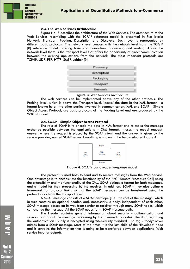
Applications of Quantitative Methods to e-Commerce
226
2.3. The Web Services Architecture Figure No. 3 describes the architecture of the Web Services. The architecture of the
Web Services resembling with the TCP/IP reference model is presented in five levels: Network, Transport, Packing, Description and Discovery. Each level is represented by different basic protocols. The network level concurs with the network level from the TCP/IP [8] reference model, offering basic communication, addressing and rooting. Above the network level there is the transport level that offers the opportunity of direct communication between the existing applications from the network. The most important protocols are TCP/IP, UDP, FTP, HTTP, SMTP, Jabber [9].
Figure 3. Web Services Architecture
The web services can be implemented above any of the other protocols. The Packing level, which is above the Transport level, "packs" the data in the XML format – a format known by all the other parties involved in communication. XML and SOAP – Simple Object Access Protocol, are basic protocols of the Packing Level and are produced by the W3C standard.
2.4. SOAP – Simple Object Access Protocol The role of SOAP is to encode the data in XLM format and to make the message
exchange possible between the applications in XML format. It uses the model request-answer, where the request is placed by the SOAP client, and the answer is given by the service provider, named SOAP server. Everything is shown in the below situated Figure 4.
Figure 4. SOAP’s basic request-response model
The protocol is used both to send and to receive messages from the Web Service.
One advantage is to encapsulate the functionality of the RPC (Remote Procedure Call) using the extensibility and the functionality of the XML. SOAP defines a format for both messages, and a model for their processing by the receiver. In addition, SOAP – may also define a framework for protocol links, so that the SOAP messages can be transferred using the protocol stack from the transport level.
A SOAP message consists of a SOAP envelope [10], the root of the message, which in turn contains an optional header, and, necessarily, a body, independent of each other. SOAP message passes on its way from sender to receiver through many SOAP nodes, which can change the message. All the SOAP nodes form SOAP message path.
The Header contains general information about security – authentication and session, and about the message processing by the intermediary nodes. The data regarding the authentication usually is encrypted using WS-Security standard. The tag - "body" never misses from a SOAP message. Most of the times it is the last child of the "Envelope" node and it contains the information that is going to be transferred between applications (Web service input or output).

Applications of Quantitative Methods to e-Commerce
227
In Figure 5 it is shown an example of a SOAP message.
Figure 5. SOAP Message
In the above example, in the SOAP envelope the XML namespace and the type of
the used message encoding are not specified. The Header node is missing in this example, and the body node contains the result of a "GetMaterials" method, which is a serialized Data Table type object in XML format.
SOAP was originally an acronym for Simple Object Access Protocol, But since SOAP Version 1.2 (SOAP 1.2 Part 0, 2003; SOAP 1.2 Part 1, 2003) it is technically no longer an acronym.
2.5. WSDL – Web Services Description Language The description level, located above the packing level, is represented by the WSDL
protocol, being based on the XML standard. WSDL is a language written in XML [11], used as a model for describing Web
services. WSDL reached version 2.0, but in version 1.1 the D stood for Definition. Version 1.2 of WSDL was renamed WSDL 2.0 because of the major differences between the two versions.
2.5.1. New features in WSDL 2.0 Nowadays, W3C recommends using WSDL 2.0 [11], but the problem is that it is not
fully supported in all developing environments. The main differences between the two versions are:
• in WSDL 2.0 there’s binding to all the HTTP request methods, whereas in WSDL 1.1 only the GET and POST methods;
• in WSDL 2.0 further semantics were added to the description language; • WSDL 2.0 offers better support for RESTful web services; • renaming of PortTypes (WSDL 1.1) into Interfaces (WSDL 2.0); • renaming of Ports (WSDL 1.1) into Endpoints (WSDL 2.0); • WSDL 2.0 can be implemented in a much simpler way.
WSDL is used in combination with SOAP and the XML schema representing the web service description. The main purpose of WSDL is that it leverages the connection between a client program and a web service, by determining the server available operations.
2.5.2. WSDL Components
Port/Endpoint – defines the address or connection to a web service; usually, it is represented by a simple URL.
Service – consists of a set of ports/endpoints, meaning the system functions exposed to the web based protocols.
Binding – defines a concrete message format and transmission protocol which may be used to define a port/endpoint.
PortType/Interface – defines a web service, all the operations that can be performed, and the messages used to perform the operation.
Operation – is an interaction with the service (a method) formed by a set of messages exchanged between the service and the other programs involved in the interaction.
Type – describes the data type definitions that are relevant for the exchanged messages.
Components 1-3 represent the concrete section of a WSDL, and components 4-6 represent the abstract section.

Applications of Quantitative Methods to e-Commerce
228
In Figure 6 it is shown an example of a WSDL message.
Figure 6. Example of a WSDL
2.6. UDDI – Universal Description, Discovery and Integration UDDI represents a platform-independent framework [10], based on Extensible
Markup Language (XML), a directory service where businesses can register and search for web services. UDDI is meant to be open for businesses, enabling them to publish and discover services, and to discover the interaction between them over the Internet.
2.6.1. UDDI – Characteristics of UDDI [8] UDDI stores information about web services, it consists of web services interfaces
written in WSDL. UDDI can be interrogated via SOAP messages and provides access to WSDL documents describing certain protocol bindings and message formats to interact with the web services. UDDI terminology contains also the following:
• Nodes – servers which support UDDI specifications nodes belong to a registry;
• Registries – collections of one or more UDDI nodes.
2.6.2. Benefits of UDDI All businesses can benefit of UDDI because it solves the following problems:
• Descovering the right business from millions of online businesses; • Once the preferred business is discovered, UDDI enables how to enable
commerce; • New customers cand be reached and access to current customers can be
increased; • Market reach and offerings can be expanded; • Barriers are removed to allow rapid participation in the global Internet
economy; • Services and business processes are programatically described in a single,
open, and secure environment.

Applications of Quantitative Methods to e-Commerce
229
In Figure 7 it is shown an example of a UDDI message.
Figure 7. Example of a UDDI Although the basic specifications of Web Services: XML, SOAP, WSDL and UDDI
provide an acceptable level of interoperability and integrity [11] a significant effort has made to increase the applications area of Web Services, and to address to higher various issues from the real world. Thus new specifications emerged for Web Services’ reliability, security, metadata management, transactions and orchestration, all of which have extended the Web Services’ architecture. Among the new specifications it is worth to be mentioned:
• Metadata Management: WS-Addressing, WS-Policy, WS-MetadataExchange; • Reliable Messaging: WS-Reliability, WS-ReliableMessaging, WS-Eventing,
WS-Notifications; • Security: WS-Authorization, WS-SecurityPolicy, WS-Trust, WS-
SecureConversation, WS-Federation, WS-Privacy, XML Encryption, XML Signature; • Transactions: WS-Transactions family(WS-AtomicTransaction, WS-
BusinessActivity, WS-Coordination), WS-Composite Application Framework( WS-CAF); • Orchestration • Choreography
3. Case study regarding the integration of Web Services on different platforms
This section describes a case study on web services and associated key technologies, offering practical tests in order to support the previous presented. The application shows how to integrate Web Services on different platforms and how they allow the interoperability between applications running on these platforms, using the specific web services protocol stack presented in previous sections.
The problem we have modeled is as follows: "A company that sells used hardware in the fields of retail and food industry wants to integrate some mobile terminals, which are going to be used in order to scan the bar codes of the store’s hardware equipments with an ERP system, in our case SAP."
Using a mobile terminal [12], we want to make different types of storage-specific operations, such as: reception, delivery and material’s inventory.
The solution we present for integrating the mobile devices with SAP - consists in developing a web service on a .NET platform, that can be used as a proxy between the two platforms.

Applications of Quantitative Methods to e-Commerce
230
Figure 8 presents the data flow between these distributed systems, where the interoperability occurs based on the Web services.
Figure 8. Interfacing .NET Applications with SAP via Web Services
Brief description of the scheme. Integrated with SAP Business Object Repository (BOR) [13] is an object-oriented
repository that contains SAP objects and SAP interfaces, and also their components, such as methods, attributes and events. In SAP Web Application Server, SOAP runtime provides us the mechanism of using SOAP protocol to call and access the RFC functions (Remote Function Call) [14] via HTTP. A web service in SAP can be seen as an RFC function.
The interoperability between the Microsoft .NET platform and the SAP system is done with the help of a component, the SAP Connector for Microsoft .NET [14]. It supports SAP Remote Function Call (RFC) and Web Services and it allows the development of various applications on the .Net platform. The Proxy class generation, which enables the calling for web service (RFC function) is based on WSDL. In this case, it can be said that SAP connector acts as a proxy between SAP and the .Net platform.
In order to integrate the mobile terminal with SAP, it has been developed a web service that becomes the wrapper class for the SAP connector and also it becomes a proxy between the application from the terminal and SAP.
In order to integrate the Web Service with both distributed systems some steps must be taken:
Stage 1: Developing and publishing the Web Services Using the developing platform Visual Studio.NET, a series of appropriate methods
for the data exchange is constructed. In this initial step the .Net connector is integrated to SAP. If the SAP authentication was successfully done, the description of the available RFC functions it is brought from SAP with the help of UDDI and WSDL. Since WSDL –is based on the XML standard the description of the functions is brought into a file with a .sapwsdl extension in XML format. Based on the WSDL and on the .NET connector, the proxy class, that contains the signature of the functions from the file, is being generated in order to become available for calling by other work methods.
In the example from below is shown a description of a RFC function from SAP on a proxy call basis, function that allows the over taking of the materials from the system:
/// <summary> /// Remote Function Module Z_RFC_MATERIALE. /// /// </summary> /// <param name="Gv_Eroare"></param> /// <param name="Gv_Mtart"></param> /// <param name="Gt_Matnr"></param> [RfcMethod(AbapName = "Z_RFC_MATERIALE")] [SoapDocumentMethodAttribute("http://tempuri.org/Z_RFC_MATERIALE", RequestNamespace = "urn:sap-com:document:sap:rfc:functions",

Applications of Quantitative Methods to e-Commerce
231
RequestElementName = "Z_RFC_MATERIALE", ResponseNamespace = "urn:sap-com:document:sap:rfc:functions", ResponseElementName = "Z_RFC_MATERIALE.Response")] public virtual void Z_Rfc_Materiale ( [RfcParameter(AbapName = "GV_MTART",RfcType=RFCTYPE.RFCTYPE_CHAR, Optional = false, Direction = RFCINOUT.IN, Length = 4, Length2 = 8)] [XmlElement("GV_MTART", IsNullable=false, Form=XmlSchemaForm.Unqualified)] string Gv_Mtart, [RfcParameter(AbapName = "GV_EROARE",RfcType=RFCTYPE.RFCTYPE_CHAR, Optional = true, Direction = RFCINOUT.OUT, Length = 80, Length2 = 160)] [XmlElement("GV_EROARE", IsNullable=false, Form=XmlSchemaForm.Unqualified)] out string Gv_Eroare, [RfcParameter(AbapName = "GT_MATNR",RfcType=RFCTYPE.RFCTYPE_ITAB, Optional = true, Direction = RFCINOUT.INOUT)] [XmlArray("GT_MATNR", IsNullable=false, Form=XmlSchemaForm.Unqualified)] [XmlArrayItem("item", IsNullable=false, Form=XmlSchemaForm.Unqualified)] ref ZMATNRTable Gt_Matnr) { object[]results = null; results = this.SAPInvoke("Z_Rfc_Materiale",new object[] {Gv_Mtart,Gt_Matnr }); Gv_Eroare = (string) results[0]; Gt_Matnr = (ZMATNRTable) results[1]; }
In the following example it is shown a method of web service "GetMaterials" used to call RFC function rendered above: [WebMethod] public DataTable GetMaterials() { try { string error = ""; SAPProxy proxy = new SAPProxy(this.BuildConnectionString()); ZMATNRTable materialsERSA = new ZMATNRTable(); proxy.Z_Rfc_Materiale("ERSA", out error, ref materialsERSA); if (error != String.Empty) throw new Exception(error); Access access = new Access(ConfigurationManager.ConnectionStrings["ConnectionString"].ConnectionString); for (int i = 0; i < materialsERSA.Count; i++) access.SynchronizeMaterials(materialsERSA[i], "ERSA"); return materialsERSA.ToADODataTable(); } catch (Exception exc) { throw (exc); } }
Stage 2: Rendering the Web Service At this stage, after the construction of the web service, it will be rendered in the
application from the mobile terminal which is developed on the .Net platform. If the service is available, similar to Stage 1, the description of the service in the application is brought with the help of UDDI and WSDL.

Applications of Quantitative Methods to e-Commerce
232
Stage 3: Calling methods of service After rendering the contract and after the generation of the proxy class to call the
service, in the mobile device application one can call the service methods. Exchanging data between applications in the background, in the form of SOAP
messages is done asynchronously and at runtime. If there is a large volume of data, due to the interoperability based on XML standard, the process may be slowed because of the need for parsing of the XML messages in different types of objects. This exchange of messages is done by following these steps:
Step 1: Request the mobile application service While calling a method from the proxy class, on a SOAP framework basis, a request
is developed, in XML format. This message is attached to the SOAP - and will on a HTTP protocol basis to the service. If the service is not available and if there are no different restrictions on the network, next will be fallowed step 2, otherwise the application ends.
Step 2: Request service from SAP The request was received by the service and it will be forwarded to SAP through
connector and the proxy class. Based on the SOAP Runtime protocol, which provides access and the calling to the RFC functions, all the messages are sent in XML format via HTTP, and they are parsed as objects and BOR specific structures.
Step 3: The SAP’s answer to the service The result of the request from Step 2 is sent in XML format by the SOAP Runtime and
it is parsed by the .NET connector into the service’s specific objects.
Figure 9. Simple call web service from Windows application
Step 4: The answer of the service to the mobile application The result from Step 3, as a response from service to customer, it is sent like in Step
1. The XML message is transformed by SOAP’s framework into specific objects from the development environment, in our case a DataTable object type which can be seen in Figure 9.
4. Conclusions
Web services play a similar role with older technologies such as Remote Procedure
Call (RPC), Common Object Request Broker Architecture (CORBA), Distributed Component Object Model (DCOM), but also offers several advantages over these. The great advantage of Web Services is that they can integrate different platforms and allow the interoperability between different distributed systems. The Integrity and the interoperability can be addressed with the SOA’s help in a two-stage process that involves publishing and orchestrating the web services. The Independence with respect to various platforms is due to common standard that they all have as a basis, the XML. Using Web services provides to the developers the opportunity to create high quality applications more quickly.
In this paper, the authors came up with a pattern of using and integrating the Web services, proofing the interoperability between multiple distributed applications running on different platforms.

Applications of Quantitative Methods to e-Commerce
233
References 1. * * * Understanding Web Services http://www.webopedia.com/DidYouKnow/
Computer_ Science/2005/web_services.asp ] 2. Foster, H., Uchitel, S., Magee, J. and Kramer, J. WS-Engineer A Model-Based
Approach to Engineering Web Service Compositions and Choreography, Springer Berlin Heidelberg, 2007, pp. 87-119
3. Ciurea, C., DUMITRACHE, M. and Doinea, M. Distributed collaborative systems security, KEPT 2009 Conference The second edition, Cluj - Napoca, July 2009, pp. 20-24
4. Kovač, D. and Trček, D. Qualitative trust modeling in SOA, Journal of Systems Architecture, in Secure Service-Oriented Architectures, vol. 55, Issue 4, April 2009, pp. 255-263
5. * * * http://java.sun.com/developer/technicalArticles/WebServices/soa/ 6. Buhwan, J., Hyunbo, C., Choonghyun, L. On the functional quality of service (FQoS)
to discover and compose interoperable web services, Expert Systems with Applications, vol. 36, Issue 3, Part 1, April 2009, pp. 5411-5418
7. Ivan, I., Vintilă, B., Palaghiță, D., Pavel, S. And Doinea, M. Risk estimation models in distributed informatics applications, Globalization and Higher Education in Economics and Business Administration (GEBA 2009), Iasi, Romania, 22nd to 24th of October 2009, pp. 72-92
8. Tidwell, D. and Snell, J. Programming Web Services with SOAP, O’Reilly, 2002, 225 pp.
9. Smeureanu, A., Dumitrescu, S.D. Metode de îmbunătăţire a performanţelor aplicaţiilor GIS, Journal of doctoral research in economics, vol 1, no 1, 2009, pp. 22-29
10. Hollar, R., Murphy, R. Enterprise Web Services Security, Charles River Media, 2006, pp. 433
11. Tzima, F. and Mitkas, P. Web Services Techology, Information Science Reference, 2008, pp. 25-44
12. * * * http://sdn.sap.com 13. SAP-BC ABAP Programming Release 4.6B, SAP-AG, 2001, pp. 1540 14. Nielsen, E.S., Ruiz, S.M. and Rodriguez-Pedrianes, J. Mobile and Dynamic Web
Services, Birkhauser Verlag, Basel, 2007, pp. 117-133

Quantitative Methods Inquires
234
A STUDY ON WEIBULL DISTRIBUTION FOR ESTIMATING THE PARAMETERS
Paritosh BHATTACHARYA CEM, Kolaghat, Midnapore, India E-mail: [email protected]
Rakhi BHATTACHARJEE BITM, Shantiniketan, India
Abstract: The wind resource varies with of the day and the season of the year and even some extent from year to year. Wind energy has inherent variances and hence it has been expressed by distribution functions. In this paper, we present some methods for estimating Weibull parameters, namely, shape parameter ( k ) and scale parameter ( c ). The Weibul distribution is an important distribution especially for reliability and maintainability analysis. The suitable values for both shape parameter and scale parameters of Weibull distribution are important for selecting locations of installing wind turbine generators. The scale parameter of Weibull distribution also important to determine whether a wind farm is good or not. The presented method is the analytical methods and computational experiments on the presented methods are reported. Key words: Wind Speed; Probability Distribution; Weibull Distribution; Linear Least Square Method 1. Introduction
Today, most electrical energy is generated by burning huge fossil fuels and special
weather conditions such as acid rain and snow, climate change, urban smog, regional haze, several tornados, etc., have happened around the whole world. It is now clear that the installation of a number of wind turbine generators can effectively reduce environmental pollution, fossil fuel consumption, and the costs of overall electricity generation. Although wind is only an intermittent source of energy, it represents a reliable energy resource from a long-term energy policy viewpoint. Among various renewable energy resources, wind power energy is one of the most popular and promising energy resources in the whole world today. At a specific wind farm, the available electricity generated by a wind power generation system depends on mean wind speed (MWS), standard deviation of wind speed, and the location of installation. Since year-to-year variation on annual MWS is hard to predict, wind speed variations during a year can be well characterized in terms of a probability distribution function (pdf). This paper also addresses the relations among MWS, its standard deviation, and two important parameters of Weibull distribution.

Quantitative Methods Inquires
235
2. Weibull distribution The Weibull distribution is characterized by two parameters, one is the shape parameter k (dimensionless) and the other is the scale parameter c (m/s) The cumulative distribution function is given by
)1.....(....................exp1)(⎥⎥⎦
⎤
⎢⎢⎣
⎡⎟⎠⎞
⎜⎝⎛−−=
k
cvvF
And the probability function is given by
)2.....(..........exp)()(1
⎥⎥⎦
⎤
⎢⎢⎣
⎡⎟⎠⎞
⎜⎝⎛−⎟
⎠⎞
⎜⎝⎛==
− kk
cv
cv
ck
dvvdFvf
The average wind speed can be expressed as
)3.......()(exp)()( 1
0 0
dvcv
cv
cvkdvvvfv kk
⎥⎦⎤
⎢⎣⎡−⎥⎦
⎤⎢⎣⎡== −
∞ ∞
∫ ∫
Let k
cvx )(= ,
cvx k =
1
and dvcv
ckdx k 1)( −=
Equation (3) can be simplified as
)4...(..............................)exp(0
1
dxxxcv k∫∞
−=
By substituting a Gamma Function
( ) ∫∞
−−=Γ0
1dxxen nx into (4) and let k
y 11+= then we have
)5(........................................11 ⎟⎠⎞
⎜⎝⎛ +Γ=
kcv
The standard deviation of wind speed v is given by )6..(..........)()(0
2∫∞
−= dvvfvvσ
i.e.
)7........(.....................2)(
)(2)(
)()2(
0
22
0 0
22
0
22
∫
∫ ∫
∫
∞
∞ ∞
∞
+−=
+−=
+−=
vvvdvvfv
vdvvvfvdvvfv
dvvfvvvvσ
Use
∫ ∫ ∫ ∫∞ ∞ ∞ ∞
−− −===0 0 0 0
221
22122 )8.......()exp()()()( dxxxcdv
cv
ckxcdv
cv
ckvdvvfv kkkk
And put k
y 21+= , then the following equation can be obtained
∫∞
+Γ=0
22 )9......().........21()(k
cdvvfv

Quantitative Methods Inquires
236
Hence we get
)10.........(..........)11()21(
)11()21(
2
21
222
kkc
kc
kc
+Γ−+Γ=
⎥⎦⎤
⎢⎣⎡ +Γ−+Γ=σ
i.e. )13....(....................exp)(1
1
⎥⎥⎦
⎤
⎢⎢⎣
⎡⎟⎠⎞
⎜⎝⎛=
−
k
cv
vF
i.e. )14...(....................})(1
1ln{⎥⎥⎦
⎤
⎢⎢⎣
⎡⎟⎠⎞
⎜⎝⎛=
−
k
cv
vF
But the cumulative Weibull distribution function is transformed to a linear function like below:
Again )15.(....................lnln})(1
1ln{ln ckvkvF
−=−
Equation (14) can be written as abXY +=
where })(1
1ln{lnvF
Y−
= , vX ln= , cka ln−= , kb =
By Linear regression formula Linear Least Square Method (LLSM)
Least square method is used to calculate the parameter(s) in a formula when
modeling an experiment of a phenomenon and it can give an estimation of the parameters. When using least square method, the sum of the squares of the deviations S which is defined as below, should be minimized.
[ ]∑=
−=n
iiii xgywS
1
22 )11.......(..............................)(
In the equation, xi is the wind speed, yi is the probability of the wind speed rank, so (xi, yi) mean the data plot, wi is a weight value of the plot and n is a number of the data plot.
The estimation technique we shall discuss is known as the Linear Least Square Method (LLSM). It is so commonly applied in engineering and mathematics problem that is often not thought of as an estimation problem. The linear least square method (LLSM) is a special case for the least square method with a formula which consists of some linear functions and it is easy to use. And in the more special case that the formula is line, the linear least square method is much easier. The Weibull distribution function is a non-linear function, which is
)12(....................exp1)(⎥⎥⎦
⎤
⎢⎢⎣
⎡⎟⎠⎞
⎜⎝⎛−−=
k
cvvF

Quantitative Methods Inquires
237
)16.......(..........)(
1 1
22
1 1 1
∑ ∑
∑ ∑ ∑
= =
= = =
−
−= n
i
n
iii
n
i
n
i
n
iiiii
XXN
YXYXNb
)17.........()(
1 1
22
1 1 11
2
∑ ∑
∑ ∑ ∑∑
= =
= = ==
−
−= n
i
n
iii
n
i
n
i
n
iiii
n
iii
XXN
YXXYXa
4. Maximum Likelihood Estimator(MLE)
The method of maximum likelihood (Harter and Moore (1965a), Harter and Moore
(1965b), and Cohen (1965)) is a commonly used procedure because it has very desirable properties.
Let nxxx ...............,........., 21 be a random sample of size n drawn from a
probability density function ),( θxf where θ is an unknown parameter. The likelihood function of this random sample is the joint density of the n random variables and is a function of the unknown parameter. Thus
)18(..........),(1
∏=
=n
iiX xfL
iθ
is the Likelihood function. The Maximum Likelihood Estimator (MLE) of θ, sayθ , is the value of θ, that maximizes L or, equivalently, the logarithm of L . Often, but not always, the MLE of q is a solution of
)19.(..............................0=θd
dLogL
Now, we apply the MLE to estimate the Weibull parameters, namely the shape parameter and the scale parameters. Consider the Weibull probability density function (pdf) given in (2), then likelihood function will be
)20......())((),,,..,(1
12,1 ∏
=
⎟⎠⎞
⎜⎝⎛−
−=n
i
cx
kin
ki
ecx
ckckxxxL
On taking the logarithms of (20), differentiating with respect to k and c in turn and equating to zero, we obtain the estimating equations
∑ ∑= =
=−+=∂
∂ n
i
n
ii
kii xx
cx
kn
kL
1 1)21.(....................0ln1lnln
)22(........................................01ln1
2 =+−
=∂
∂ ∑=
n
i
kixcc
ncL
On eliminating c between these two above equations and simplifying, we get
)23...(....................0ln11ln
1
1
1 =−− ∑∑
∑=
=
=n
iin
i
ki
n
ii
ki
xnkx
xx
which may be solved to get the estimate of k. This can be accomplished by Newton-Raphson method. Which can be written in the form

Quantitative Methods Inquires
238
)24....(..............................)(')(
1n
nnn xf
xfxx −=+
Where
)25.(........................................ln11ln
)(1
1
1 ∑∑
∑=
=
= −−=n
iin
i
ki
n
ii
ki
xnkx
xxkf
And
)26......()ln)(ln1()1ln(1)(ln)('1 1 1 1
22∑ ∑ ∑ ∑
= = = =
−−−=n
i
n
i
n
i
n
ii
kiii
kii
ki xxx
nxkx
kxxkf
Once k is determined, c can be estimated using equation (22) as
)27......(....................1
n
xc
n
i
ki∑
==
5. Results and Discussions
When a location has c=6 the pdf under various values of k are shown in Fig. 1. A
higher value of k such as 2.5 or 4 indicates that the variation of Mean Wind speed is small. A lower value of k such as 1.5 or 2 indicates a greater deviation away from Mean Wind speed.
When a location has k=3 the pdf under various valus of c are shown in Fig.2. A higher value of c such as 12 indicates a greater deviation away from Mean Wind speed.
00,20,40,60,8
11,21,41,6
0 1 2 3
Probability Density
wind speed (m/s)
Fig.1 Weibull Distribution Density vers us wind speed under a constant value of c and different
values of k
k =1k =1.5k =2k =2.5k =4

Quantitative Methods Inquires
239
Fig.2: Weibull Distribution Density versus wind speed under a constant value of k=3 and different values of c
0
0.05
0.1
0.15
0.2
0 10 20 30w ind speed (m/s)
Prob
abilit
y D
ensi
ty
c=8c=9c=10c=11c==12
Fig. 3 represents the characteristic curve of .11 ⎟⎠⎞
⎜⎝⎛ +Γ
kversus shape parameter k.
The values of .11 ⎟⎠⎞
⎜⎝⎛ +Γ
kvaries around .889 when k is between 1.9 to 2.6.
Fig. 3: Characteristic curve of Г(1+1/k) versus Shape parameter k
0.88
0.9
0.92
0.94
0.96
0.98
1
1.02
1 1.5 2 2.5 3
Shape factor k
Fig.4 represents the characteristic curve of vc
versus shape parameter k .Normally
the wind speed data collected at a specified location are used to calculate Mean Wind
speed. A good estimate for parameter c can be obtained from Fig.4 as vc 128.1= where
k ranges from 1.6 to 4. If the parameter k is less than unity , the ratio vc
decrease rapidly.
Hence c is directly proportional to Mean Wind speed for 46.1 ≤≤ k and Mean Wind speed is mainly affected by c. The most good wind farms have k in this specified range and
estimation of c in terms of v may have wide applications.

Quantitative Methods Inquires
240
Fig.4: Characteristic curve of c/ṽ versus shape parameter k
0
0.2
0.4
0.6
0.8
1
1.2
0 1 2 3 4
Shape factor k
c/v
Example: Consider the following example where ix represents the Average
Monthly Wind Speed (m/s) at kolkata (from 1st March, 2009 to 31st March, 2009)
March2009 Wind Speed (m/s) March, 2009 Wind Speed (m/s)
1 0.56 17 0.28
2 0.28 18 0.83
3 0.56 19 1.39
4 0.56 20 1.11
5 1.11 21 1.11
6 0.83 22 0.83
7 1.11 23 0.56
8 1.94 24 0.83
9 1.11 25 1.67
10 0.83 26 1.94
11 1.11 27 1.39
12 1.39 28 0.83
13 0.28 29 2.22
14 0.56 30 1.67
15 0.28 31 2.22
16 0.28

Quantitative Methods Inquires
241
Also let 1
)(+
=nixF i and using equations (16) and (17) we get k= 1.013658
and c=29.9931 But if we apply maximum Likelihood Method we get k = 1.912128 and
c=1.335916. There is a huge difference in value of c by the above two methods. This is due to the mean rank of )( ixF and k value is tends to unity.
6. Conclusions In this paper, we have presented two analytical methods for estimating the Weibull
distribution parameters. The above results will help the scientists and the technocrats to select the location for Wind Turbine Generators.
References
1. Mann, N. R., Schafer, R. E., and Singpurwalla, N. D., Methods for statistical analysis of reliability and life data, John Wiley and Sons, New York, 1974
2. Engelhardt, M., "On simple estimation of the parameters of the Weibull or extreme-value distribution", Technometrics, Vol. 17, No. 3, August 1975.
3. Mann, N. R. and K. W. Fertig , "Simplified efficient point and interval estimators of the Weibull parameters", Technometrics, Vol. 17, No. 3, August 1975
4. Cohen, A. C., "Maximum likelihood estimation in the Weibull distribution based on complete and on censored samples", Technometrics, Vol. 7, No. 4, November 1965.
5. Harter, H. L. and A. H. Moore, "Point and interval estimators based on order statistics, for the scale parameter of a Weibull population with known shape parameter", Technometrics, Vol. 7, No. 3, August 1965a
6. Harter, H. L. and A. H. Moore, "Maximum likelihood estimation of the parameters of Gamma and Weibull populations from complete and from censored samples", Technometrics, Vol. 7, No. 4, November 1965b
7. Stone, G. C. and G. Van Heeswijk, "Parameter estimation for the Weibull distribution”, IEEE Trans. On Elect Insul. VolEI-12, No-4, August, 1977.
8. P. Gray and L. Johnson, Wind Energy System Upper Saddle River, NJ: Prentice-Hall, 1985

Quantitative Methods Inquires
242
MINIMIZATION, CONSTRAINTS AND COMPOSITE
BÉZIER SURFACES1
Arie JACOBI2 Department of Software Engineering, Sami Shamoon Academic College of Engineering, Beer Sheva, Israel E-mail: [email protected]
Shilo LIFSCHUTZ3 Department of Accounting, Academic Center of Law and Business, Ramat-Gan, Israel E-mail: [email protected]
Abstrct: This paper presents a global method for approximation and/or construction of surfaces using constraints. The method is based on a min max problem which describes approximation and differential geometric characteristics, constrained in order to achieve desired geometrical effects. The numerical solution of the problem takes full advantage of the Finite-Elements method and of constrained optimization algorithms. Key words: Bézier surface; Offset surface; Surface Fitting; Offset Surface; Approximate Conversion; surface approximation; Surface simplification; Variational Problem Formulation; Finite-Element Method (FEM); FEM’s hp-method; Lagrange Multipliers Formulation
1. Introduction Approximation of surfaces and construction of offset surfaces has a variety of
applications. For example: • Approximation to a set of scattered points in three-dimensional space
originated from scientific experiments, earth terrain description, or data from satellites • Exchanging format of formal data. It is required in geometric modeling
systems for free form surfaces, as they use different mathematical representations and different polynomial bases for curves and surface representation
• Conversion between non-polynomial representations (such as rational surfaces) to polynomial ones.
Additional motivations for approximation are the ability of merging curves and
surfaces in order to reduce information or the construction of offset curves and surfaces which are needed in tool paths planning for numerical control machines and in construction of a thick surface that is used as the outer (or inner) surface of objects such as, a car, an airplane, or a mold.

Quantitative Methods Inquires
243
Finite element methods are an essential tool for the approximation of a solution of a partial differential equation and are based on the weak variational formulation of boundary and initial value problems. The importance of this property is twofold:
• It provides the proper setting for the existence of a very irregular solution to differential equations.
• The solution appears in the integral of a quantity over a domain, which can be broken up into the sum of integrals over an arbitrary collection of almost disjoint sub-domains whose union is the original domain.
These properties allow analysis to be done locally on a typical sufficiently small
sub-domain, so that polynomial functions of various degrees are adequate for representing the local behavior of the solution (see [27]). In order to arrive at a global approximation of a solution of a partial differential equation in the finite element method, their contributions of local approximation over individual elements are assembled together in a systematic way. This leads to schemes which are robust in appropriate norms and insensitive to distortions and singularities of the mesh.
Desirable Properties of an Approximation Surface
We consider the following properties for curve approximation and construction: • End Points Interpolation - The approximation surface’s end points should
interpolate the approximated surface’s end points. • End Directions Preservation - The approximation surface’s boundary curves’
end tangents should have the same direction as the approximated surface’s boundary curves’ end tangents.
• Parametric and Geometric Continuity - Creation of a smooth approximation surfaces. There are cases where a higher parametric continuity degree ( or ) between the approximation surface patches is needed. It is also possible to ensure geometric continuity of first degree ( ) between the approximation surface patches.
2. Previous Work There are several approaches for approximation of curves, surfaces, or points in
three-dimensional space. Among the early important works in this field for the approximate conversion of curves and surfaces as well as the construction of offset curves and offset surfaces, we would like to signify the works of [11,26] and [16]-[24]. Among the recent works there is the work of Weiss et al. [30], that attempts to provide practical solutions to overcome problems of irregular distribution of data points which are over topologically irregular domains. The Weiss et al. method includes algorithms to compute a good initial parametrization, a procedure for handling weakly defined control points, a shape dependent knot refinement, and a fitting strategy to maintain tight tolerances and smoothness simultaneously. Their method achieves a high accuracy relative to the published ‘standard’ solutions.
Borges and Pastva [9] deal with the problem of fitting a single Bézier curve segment
to a set of ordered data so that the error is minimized in the total least squares sense. They developed an algorithm for applying the Gauss–Newton method to this problem with a direct method for evaluating the Jacobian based on implicitly differentiating a pseudo-inverse. Chen Guo-Dong and Wang Guo-Jin [10] consider simultaneous fitting of multiple curves and surfaces to 3D measured data captured as part of a reverse engineering process, where constraints exist between the parameters of the curves or surfaces. Enforcing such constraints may be necessary
• to produce models of sufficiently accurate tolerances for import into a CAD system, and

Quantitative Methods Inquires
244
• to produce models which successfully reproduce regularities and symmetries required by engineering applications.
There are several works in the CAGD field that use Bernstein-Bézier finite elements
in the context of approximation. One of the earliest works on actual approximate conversion is Bercovier and Jacobi [3, 4] and Luscher [25]. Examples of later works that use FEM in CAGD are hierarchical methods for linear spline approximation and construction of surface triangulations or quadrangulations by adaptively subdividing a surface to a form of tree. It is used in an approximation to a set of scattered points in three-dimensional space using hierarchical spline and surface approximation methods such as in [8], or for approximation over irregular domain as introduced in [5, 6, 7, 31]. An implementation of cubic tetrahedral Bernstein-Bézier finite elements and their application in the context of facial surgery simulation is presented in [28]
3. Our Approach and its Strategy Our approach uses the combination of the finite element method with the
Bernstein-Bézier representation, introducing a valuable finite element due to the many advantages of the Bernstein-Bézier shape functions [14]. It introduces the construction of surfaces given by piecewise definitions of their parameter range and allows surface editing, both in the direction of several (lower order) surfaces approximating a single given one, or, conversely replacing several by a single one. This approach exploits the p-method and the h-method in FEM in order to improve approximation. This is done by using elements of higher degrees to overcome areas that are difficult to approximate and by using elements with lower degrees for approximating the rest of surface for implementing the p-method. For the implementation the h-method we use element mesh which is refined to increase accuracy. In order to achieve desired geometrical properties for the approximation surface, we incorporate parametric ( - ) and geometric ( ) continuity constraints between the approximation surface patches, and other constraints, such as a constraint for the interpolation of the approximation surface end points with the end points of the given surface, or, a constraint to enforce the directions of the end edges of each boundary curve control polygon of the approximation surface to have the same directions as the tangents at the end points of the approximated surface boundary curves.
The strategy we use (see [3, 4]) is a global and continuous method for the
approximation and construction of parametric surfaces. The method is based on a variational formulation which includes geometrical relations between surfaces and constraints upon the geometry and/or parameterization of the approximation surface. The variational formulation is based on the squared integrals of the zeroth, first, and second derivative (semi) norms of the approximation and approximated surfaces. We introduce the Lagrangian multiplier formulation for the constraints implementation. A weighting factor is related to each derivative (semi) norm. These weighting factors allow one to control the approximation of the related norm. The solution of this constrained variational problem is done by the Finite Element Method (FEM) over Bernstein basis functions.
Outline of this Paper
Description of the unconstrained problem, the constrained problem and its solution, is presented in sections 2-4. In section 5, a survey of the methods for estimating the approximation errors is given. Section 6, introduces the constraints we use to improve the approximation. A number of examples involving constraints, for surface degree reduction, surface merging and construction of offset surfaces are shown in section 7.

Quantitative Methods Inquires
245
4. The Problem
Problem Statement
We will first define the problem without constraints. Given a parametric surface: find the unknown vector function
which is the solution by minimization, of one of the following three related
problems we consider in this article: (1) (2)
(3) where
(4)
(5) and
(6) are the zeroth, first, and second error (semi) norms, respectively, and , , and
positive moduli which are used as weighting factors.
Solution for the Problem Using the FEM Technique
In the following section we present the solution of the problem stated in section 2.1 using the FEM technique. The solution process includes: the partition of the problem’s domain into two-dimensional elements, the calculation of a stiffness matrix and load vector for a given element , the assembly of the elements’ stiffness matrices and load vectors into the main stiffness matrix and load vector, and the calculation of the approximation error. The solution to one of the problems (1-3), follows the Galerkin-Ritz solution scheme (a computational example for the Rayleigh-Ritz and Galerkin methods, using the strong form of Poisson’s equation can be seen in [29]).
The Approximation FEM Space
Given the partition:
(7) of the rectangular range (8) each sub-range (9) for is the global parameter range of an
element , where and is the number of elements.

Quantitative Methods Inquires
246
We use the following linear transformation to establish the relation between the
global parameters and the local parameters :
(10)
where
(11)
We introduce an dimensional approximation space , consisting of
functions which are piecewise Bézier patches over the range . Let
(12)
We define
(13)
to be the minimization space, where is the finite-dimensional subspace (12) of .
Problem Description for a given element
Using partition (7) and given element , where and is the number of elements, we set:
(14)
(15) and
(16) to be the zeroth, first, and second error (semi) norms for the element , and for the
element sub-range (as in (9)), respectively.

Quantitative Methods Inquires
247
Let
(17)
where (18) or,
(19)
where for the -th element, is the vector of the unknown Bézier points, is the element load vector and
is the element stiffness matrix. Our objective is to find for all the function which is taken over the
space , in order to approximate in some sense to be defined later.
General Solution of the Problem
After integration element by element, we obtain:
(20)
or
(21)
The elements’ stiffness matrices , and load vectors , , are assembled into the global stiffness matrix and load vector .
The minimum of each in (21), is given by the approximation surface ,
where is the solution of the system (22) The system (22) is linear symmetric positive definite, and we use the
algorithm or the Conjugate-Gradient [32] to solve it. The coordinate components of are decoupled, and the solution of the system refers to each coordinate component by itself.
Properties of the Global Stiffness Matrix The global stiffness matrix is sparse, square banded, symmetric and positive
definite. All of its elements are positive, the largest element per row or column is in the main diagonal, and the sum of all elements in a row (or in a column), is constant for each n. Its graph’s shape is determined by the numbering of each of the degrees of freedom involved in the problem.
Let, • be the sum of degrees of freedom for all the
elements, • ElementsAlongU, ElementsAlongV be the number of elements along u and v
parameter lines respectively, • and NodesAlongU, NodesAlongV be the number of nodes along u and v
parameter lines respectively (every node contains 3 degrees of freedom).

Quantitative Methods Inquires
248
For each element of degrees , there are degrees of
freedom. Every boundary curve which shares two neighboring elements (patches) decreases the total number of degrees of freedom by:
Every cross section of such two boundary curves (meaning, at a cross section of four
neighboring elements) decreases the total number of degrees of freedom by . The total sum of degrees of freedom at the cross sections is:
Therefore, the total number of the problem’s degrees of freedom and the order of
the global stiffness matrix is at most . The creation of the global stiffness matrix is fast and efficient, since it involves only the assembly of the element stiffness matrices, which are pre-calculated and small.
The constrained Problem and its solution
Among the exiting numerous algorithms for solving a constrained optimization
problem, some solve the constrained problem by replacing it with a family of unconstrained optimization problems. We use the Lagrangian multiplier formulation that converts the constrained minimization problem,
into the following unconstrained min max problem,
(23)
where (24)
is called the Lagrange multiplier for the constraint . Solution of problem (23) with regard to the degrees of freedom in and yields the following necessary conditions:
(25)
Error Estimation
Since the approximation depends on the parametrization of and , it
does not necessarily yield orthogonal error vectors between corresponding values of parameters. The absolute Euclidean minimum (or maximum) is at the point where two normals are collinear. Therefore a re-parametrization is needed so that the correction of the parametrization will direct the error vectors to be as orthogonal as possible to the tangent plane of at . This will result in a better error estimation [16].
We use two types of discrete error estimators: • the largest error Euclidean distance : (26)

Quantitative Methods Inquires
249
• the maximal angle deviation , between the normals:
(27) In order to use error measurements which are not dependent on the
parametrization, we use the zeroth, first and second derivative error (semi) norms (4-6) for error estimation. The zero derivative error norm (squared error integral) is the norm. The first and second derivative error (semi) norms are used to estimate the error in the first and second partial derivatives displacements.
We also use the error (semi) norms , and , which
measure the mean error displacement per unit area, where is an approximated area of . For error in curvature, we use the Gaussian curvature error norm:
(28)
where is the Gaussian curvature of the approximated surface , and the Gaussian curvature mean deviation error:
(29)
We also use the mean curvature error norm:
(30)
where is the mean curvature of the approximated surface , and the mean curvature mean deviation error:
(31)
Error estimations of all types presented in this section are presented in tables 1-2, for the approximation of a Bézier patch of degrees 5 x 3, with sizes of 3 x 28.5 and approximated area of (see Figure 1), by a Bézier patch with different degrees and continuity orders between elements.
degrees segments
2 x 3 1 x 1 1.479 0.348 2.348264e-04
2.523826e-05
5.107362e-05
3 x 3 1 x 1 0.380 0.240 1.465209e-05
1.818131e-06
5.128979e-05
4 x 3 1 x 1 0.365 0.220 1.395186e-05
1.595004e-06
1.254311e-05
5 x 3 1 x 1 0.0 1.13e-07 4.447024e-19
2.911940e-18
1.115636e-04
3 x 3 2 x 1 0.450 0.245 1.396280e-05
2.934349e-06
1.763063e-04
4 x 3 2 x 1 0.041 0.039 1.395732e-07
7.531847e-08
1.712148e-04
2 x 3 3 x 1 0.540 0.276 1.530292e-05
2.978221e-06
1.713536e-04
3 x 3 3 x 1 0.051 0.058 1.651474e-07
1.487066e-07
1.769908e-04

Quantitative Methods Inquires
250
4 x 3 3 x 1 0.002 0.006 5.137242e-10
2.253008e-09
1.929809e-04
4 x 3 3 x 1 0.002 0.005 4.885186e-10
1.619946e-09
1.930424e-04
4 x 3 3 x 1 0.011 0.001 8.110637e-09
8.997212e-09
1.935975e-04
Table 1: Various error estimations by the derivative error (semi) norms, for the approximation of a Bézier patch of degrees 5 x 3, with sizes of 3 x 28.5 and approximated area of , by a Bézier patch with different degrees. See Figure: 1
degrees 2 x 3 3.339768e+00 9.764867e-01 5.592338e+00 8.735588e-01 3 x 3 2.059826e+00 5.233216e-01 3.087451e-01 5.079714e-02 4 x 3 6.194731e-01 1.573840e-01 2.562805e-01 4.216526e-02 5 x 3 2.012408e-14 5.084107e-15 1.561175e-14 2.442805e-15 3 x 3 8.055888e-01 3.363193e-01 3.795821e-01 5.976159e-02 4 x 3 8.473989e+00 3.537743e+00 8.030403e-02 1.264311e-02 2 x 3 4.354274e-01 5.014103e-01 4.724982e-01 7.439097e-02 3 x 3 1.259487e+01 1.449829e+01 1.270752e-01 1.998752e-02 4 x 3 8.319730e+01 9.577063e+01 6.819476e-01 1.072628e-01 4 x 3 8.309422e+01 9.565197e+01 6.816075e-01 1.072093e-01 4 x 3 8.281638e+01 9.533215e+01 6.837922e-01 1.075529e-01
Table 2: Various error estimations by the curvature error norms, for the same given Bézier patch and approximation surfaces as in Table 1.
(a) Given surface (b) The approximation surface.
Figure 1: Reduction of a Bézier patch of degrees (5 x 3), with sizes of 3 x 28.5 and approximated area of , by an approximation ( ) Bézier surface with three
patches of degrees (4 x 3).

Quantitative Methods Inquires
251
5. Incorporation of Constraints In this section we introduce the description and implementation of constraints
which are imposed upon the approximation or the construction of surfaces in order to achieve the following desired geometrical effects:
Constraints for Surface’s End Points Interpolation
In order to create a better approximation, the end points of the approximation surface should interpolate the end points of the given surface. Meaning, the conditions:
(32) must be satisfied.
First Derivative Interpolation at the End Points of Boundary Curves
The direction of the end edges of each boundary curve control polygon of the approximation surface, are constrained to have the same directions as the tangents at the end points of the approximated surface boundary curves. The method used for this constraint, is the same one used for curves, as described in [4].
Constraints for , Continuity Between Elements
Higher continuity between elements will not necessarily improve the approximation but will create a smoother approximation surface, a feature which is desirable in many cases, such as, the design of mechanical parts which requires first- or second- order smoothness, or in the definition of a tool path for NC machine where we need the speed and the acceleration of the tool to be continuous. This can be achieved by and parametric continuity.
A Bézier surface may contain several patches joined together with a given
continuity. Let and be two Bézier patches defined over and respectively. and have
continuity along the parametric line , if
(33)
For Bézier surfaces it is possible to reduce the surface problem to several curve problems. Using the cross boundary derivative (the derivative at the common boundary curve) with respect to the global parameters we obtain:
(34)
It follows that along the parametric line ,
(35)
Equations (35) are conditions on rows of control points across the boundary curve which represents Bézier curves (see [14,23]).
The continuity constraints can be imposed only on part of the patches. This is usually done on a boundary of complete two rows or two columns in the mesh of elements. This way we construct a surface the in some parts it has a high continuity degree ( for example), and in other parts a continuity is left to produce a corner or a cusp.
Examples
Approximation of surfaces can be used in the applications of: degree reduction of surfaces, merging of surfaces with large number of patches, and construction of offset

Quantitative Methods Inquires
252
surfaces. Reduction of degree of high order polynomial surfaces to polynomials of a lower order. The degree reduction approximation might reduce or increase the number of surface patches. It is sometimes needed to merge a surface which is constructed from many small patches into a surface with less patches of the same degrees, or even with higher degrees. The construction of a parametric offset surface, is done by approximating the offset surface
to the given surface . (36) where is the principal normal vector, and is the offset distance along
. Among the surfaces that we used in the section, there are the following three
surfaces: 1. The surface BRODE (Fig. 2(a)), which is a 9 x 9 Bézier patch with sizes of 100
x 140 mm. 2. The surface SEITE1(Fig. 2(b)), which is a collection of 9 x 7 Bézier patches,
each of degrees 3 x 3 and sizes about 500 x 2200 mm. 3. The surface SURFB (Fig. 2(c)), which is a collection of 17 x 63 Bézier patches,
each of degrees 5 x 5 and sizes about 450 x 1800 mm. These surfaces were used as test examples (bench-mark) for the comparison
between spline conversion methods (See for example, [12, 13, 15, 24]. The bench-mark specifications were to convert these surfaces to a 3 x 3 or a 5 x 5
Bézier or B-Spline surface with a maximal error tolerance of 0.1 and 0.01 . For each of the surfaces involved in the bench-mark a table was presented, in which the degrees and the segment number of the result approximation surface are listed in the first two columns. In the third column the inner continuities in both parameter directions are entered. The fourth column contains the compression factor. The compression factor for the conversion to Bézier surface is given by the quotient:
and the compression factor for the conversion to B-Spline surface is given by the quotient:
In the fifth column the approximation presents the prescribed approximation
tolerance, and in the sixth column the largest error Euclidean distance is given. We will use the same format of table for our examples.
(a) The BRODE surface (b) The SEITE1 surface

Quantitative Methods Inquires
253
(c) The SURFB surface
Figure 2 : Benchmark Surfaces.
Constraints results
Examples of constrained approximations are introduced in our results of the bench-mark surfaces BRODE, SEITE1 and SURFB in tables (3-5). These examples emphasize the p-method and h-method of FEM in the approximation. We see for example in table (5) that presents approximation results for the SURFB surface (Figure 2(c)), that each line in the table introduces an approximation with a different mesh size (signified by the segments column of the table) and patch degrees. One can see the different continuity degrees achieved by the imposing or continuity constraints between the approximation surface patches. The last two lines of table (3), represent an approximation of the BRODE surface (Figure 2(a)), that uses a mesh of elements of different degrees, attached with continuity. These results display how the combination of the hp-methods in FEM was used in the approximation scheme of this research.
Another example that displays an approximation of an offset surface is presented in figure (3). The approximation offset surface that approximated a surface of degrees (3 x 3) (Figure 3(a)), has an offset distance of -0.4 , two patches of degrees (3 x 3) and ( continuity between its patches. The approximation integrates the end points and first derivative interpolation constraints.
All the above examples integrated the end points and first derivative interpolation constraints (see sections 6.1-6.2, respectively).

Quantitative Methods Inquires
254
Table 3. surface: BRODE: surface: BRODE: degree: 9 x 9, segments: 1 x 1
degree segments minimal compression error measured continuity factor tolerance error 3 x 3 5 x 3 0.42 0.01 0.008 3 x 2 1.04 0.01 0.01 2 x 2 1.56 0.1 0.042 3 x 2 1.04 0.1 0.018 4 x 3 2 x 2 1.25 0.1 0.017 4 x 4 2 x 2 1.0 0.01 0.006 2 x 1 2.0 0.1 0.026 4 x 5 2 x 1 1.66 0.1 0.016 5 x 3 1 x 2 2.08 0.1 0.023 5 x 5 2 x 2 0.69 0.01 0.002 2 x 1 1.39 0.1 0.015 1 x 1 2.78 0.1 0.022 7 x 6 1 x 1 1.79 0.1 0.004 7 x 7 1 x 1 1.56 0.1 0.001 3,5,3 x 3,4 3 x 2 1.04 0.01 0.008425 3,3,2,2,3,3 x 3,4 6 x 2 0.52 0.01 0.009057
Table 4. surface: SEIT1
urface: SEITE1: degree: 3 x 3, segments: 9 x 7 degree segments minimal compression error measured continuity factor tolerance error 3 x 3 8 x 7 1.13 0.01 0.0088 2 x 7 4.5 0.1 0.1 4 x 3 2 x 7 3.6 0.1 0.068960 5 x 3 3 x 7 2.0 0.01 0.003987 5 x 5 3 x 7 1.33 0.01 0.003985 2 x 7 2.0 0.1 0.023714 1 x 7 4.0 0.1 0.1
Table 5. surface: SURFB
surface: SURFB: degree: 5 x 5, segments: 17 x 63 degree segments minimal compression error measured continuity factor tolerance error 3 x 3 17 x 29 4.89 0.01 0.008632 17 x 16 8.86 0.1 0.076872 3 x 4 17 x 13 8.72 0.1 0.016416 3 x 5 17 x 13 7.27 0.01 0.004687 17 x 8 11.81 0.1 0.041205 4 x 4 14 x 17 6.48 0.01 0.008888 8 x 11 17.53 0.1 0.079889 5 x 4 6 x 11 19.47 0.1 0.095811 5 x 5 14 x 13 5.88 0.01 0.008055 6 x 6 29.75 0.1 0.075385

Quantitative Methods Inquires
255
(a) Bézier patch of degrees (b) The shaded surfaces
Figure 3: An offset Bézier surface to the surface (a), with two patches of degrees , ( continuity between patches and offset length of -0.4.
6. Conclusions and Future Work In our work we introduced a global and continuous method for approximation
and/or construction of surfaces. It is based on a minimization of a functional which makes use of global and continuous criteria (4-6), for approximation and construction. Constraints were integrated in the approximation to obtain some specific characteristics. Some of the properties we would like to obtain are aimed at improving the approximation, such as, end points interpolation and end direction preservation. Others are designed to impose a desirable form upon the approximation surface, for instance, parametric continuity between the approximation surface’s patches. The constraints used were linear, equality, and operates on a discrete parameter range. We used the Lagrangian multiplier formulation for the constrained problem.
The numerical solution of the functional uses FEM with the Bernstein-Bézier
representation for the shape functions, and presents cardinal advantages: • The approximation method operates globally on the given problem’s
domain. • Segmentation of the approximation surface is natural to FEM, because of the
subdivision of a FEM problem’s domain into elements.
(c) The shaded surfaces (d) The surfaces with drawing of the tangents along the v-parameter lines

Quantitative Methods Inquires
256
• Every element is treated separately, and its "influence" is added to the general stiffness matrix such that there is no limitation on the form of the general range combined from a collection of elements.
• It is possible to approximate, using different elements with different degrees of elements (Bézier patches).
• The system of equations is linear for any degrees of the elements and any order of parametric continuity between the elements.
• The use of Bézier-Bernstein representation grants good properties for the stiffness matrix, and saves much of the approximation calculation using proper solution methods (such ). Most of the calculation of the element matrices is prepared in advance and can be used regardless of the subdivision of problem’s domain.
• There is not a pre-requirement on the given surface’s continuity. • It is possible to approximate, using different elements with different degrees
of parametric continuity, including . As the next step in this research, we intend to include different types of linear and
nonlinear constraints, of equality and/or inequality types, on a discrete or a continuous parameter range. These constraints are aimed at improving the approximation, or at imposing a desirable form upon the approximation surface. Examples of such constraints are, optimal construction using reparametrization, opening loops for given looped surfaces, or avoiding loops in the approximation of offset surfaces. References
1. Babuska, I., Szabo, B.A. and Katz, I.N. The p-version of the Finite Element Method,
SIAM J. Numerical Analysis, No. 18, 1981, pp.515-545 2. Babuska, Ivo and Suri Manil The P and H-P Versions of the Finite Element Method,
Basic Principles and Properties, SIAM Review, Vol. 36, No. 4, Dec. 1994, pp. 578-632
3. Bercovier Michel and Jacobi Arie Approximation and/or Construction of Curves by Minimization Methods with or with-out Constraints, MAN Mathematical Modelling and Numerical Analysis, Vol. 26, No. 1, 1992, pp.211-232
4. Bercovier Michel and Jacobi Arie Minimization, Constraints and Composite Bézier Curves, Computer Aided Geometric De-sign - Computer Aided Geometric Design, Vol: 11, 1994, pp. 533-563
5. Bercovier, M., Volpin, O. and Matskewich, T. Globally G1 Free Form Surfaces using ”Real” Plate Energy Invariant Energy Methods, Curves and Surfaces with Applications in CAGD, 2, 1997
6. Matskewich, T., Volpin, O. and Bercovier, M. Discrete G1 Assembly of patches over irregular meshes, Proceedings of Curves and Surfaces in CAGD, Norway, 1997
7. O. Volpin and M. Bercovier Generation of Quadrilateral meshes from triangular data with resulting smooth surface reconstruction, Proc.IEEEConf.InformationVisualisation-IV98,London, 1998, online source: http://www.computer.org/proceedings/IV/8509/
8. Bercovier, M. and Volpin, O. Hierarchical Bezier Surfacee over Arbitrary Meshes, Computer Graphics Forum,18(4), 1999, pp. 223-236
9. Borges F.and Pastva T. Total least squares fitting of Bézier and B-spline curves to ordered data, Computer Aided Geometric Design, Vol. 19, No. 4, 2002, pp. 275-289
10. Chen Guo-Dong and Wang Guo-Jin Optimal multi-degree reduction of Bézier curves with constraints of endpoints continuity, Computer Aided Geometric Design, Vol. 19, No. 4, 2002, pp. 275-289
11. Dannenberg, L.; Nowacki, H. Approximate Conversion of Surface Representations with Polynomials Bases, Computer Aided Geometric Design, No. 2, 1985,

Quantitative Methods Inquires
257
pp. 123-132 12. Dokken, T. and Lyche, T. Spline Conversion: Existing Solutions and Open
Problems, In: Laurent, P.J. and M´ehaut´e A.L. and Schumaker L.L. Curves and Surfaces in Geometric Design, A K Peters, Wellesley, 1994, pp. 121-130
13. Eck, M. and Hadenfeld, J. A Stepwise Algorithm for Converting B-Splines, In: Laurent, P.J. and Mehaute A.L. and Schumaker L.L. Curves and Surfaces in Geometric Design, A K Peters, Wellesley, 1994, 121-130
14. Farin, G. Curves and Surfaces for Computer Aided Geometric Design, A Practical Guide, Academic Press, Inc., Boston, 3rd Ed, 1988
15. Goult, R. J. Applications of Constrained polynomials to Curve and Surface Approximation, In: Laurent, P.J. and Mehaute A.L. and Schumaker L.L. Curves and Surfaces in Geometric Design, A K Peters, Wellesley, 1994, pp. 217-224
16. Hoschek, J. O set Curves in the Plane, Computer Aided Design, No. 4, 1985, pp. 59-66
17. Hoschek, J. Approximation Conversion of Spline Curves, Computer Aided Geometric Design, No. 17, 1987, pp. 77-82
18. Hoschek, J. Spline Approximation of O set Curves, Computer Aided Geometric Design, Vol. 5, 1988, pp. 33-40
19. Hoschek, J. Intrinsic Parameterization for Approximation, Computer Aided Geometric Design, Vol. 5, 1988, pp. 27-31
20. Hoschek, J., Schneider, F. J. and Wassum, P. Optimal Approximation Conversion of Spline Surfaces, Computer Aided Design, No. 20,1988, pp. 457-483
21. Hoschek, J. and Wissel, N. Optimal Approximate Conversion of Spline Curves and Spline Approximation of O set Curves, Computer Aided Design, Vol. 20, No. 8, 1988, pp. 475-483
22. Hoschek, J. and Schneider, F.J., Spline Conversion for Trimmed Rational Bézier- and B-Spline Surfaces, Computer Aided De-sign, Vol 22, No. 9 (1990), pp. 580-590.
23. Hoschek, J. and Lasser, D. Computer Aided Geometric design, A K Pters, Wellesley, 1993
24. Hoschek, J. and Schneider, F.J. Approximate Conversion and Data Compression of Integral and Rational B-splne Surfaces, In: Laurent, P.J. and Mehaute A.L. and Schumaker L.L. Curves and Surfaces in Geometric Design, A K Peters, Wellesley, 1994, pp. 241-250
25. Luscher, N. The Bernstein-Bézier Technique in the Finite Element Method, Exemplary for the Univariate Case, Technical Report from the University of Braunschweig, 1988
26. Nowacki, H., Dingyuan, L. and Xinmin, L. Fairing Bézier Curves With Constraints, Computer Aided Geometric Design, No. 7, 1990, pp. 43-55
27. Oden J. Tinsley Finite Elements: An Introduction, In: Ciarlet P.G. and Lions J.L., editors, Handbook of Numeri-cal Analysis. Finite Element Methods (Part 1), Vol. II, North-Holland, 1991
28. Roth, S. H. M. BernsteinBézier Representations for Facial Surgery Simulation, A thesis dissertation submitted to the Swiss Federal Institute of Technology, ETH, Zurich, 2002
29. Strang, G. Introduction to Applied Mathematics, Wellesley-Cambridge Press, 1986 30. Weiss, V., Andorb, L., Rennera, G. and Veradya, T. Advanced surface fitting
techniques, Computer Aided Geometric Design Vol. 19, No. 1, 2002, pp. 19-42
31. Xiquan Shi, Tianjun Wang and Piqiang Yu A practical construc-tion of G1 smooth biquintic B-spline surfaces over arbitrary topology, Computer-Aided Design, 36, (2004), 413424
32. Zienkiewicz, O. C. The Finite Element Method in Engineering Science, McGraw-Hill, London, 1971

Quantitative Methods Inquires
258
1 Acknowledgments This research was partially supported by a grant from the Ministry of Science and Culture, Land Hessen, W. Germany 2 Arie Jacobi is Senior Lecturer in the Software Engineering Department, Sami Shamoon College of Engineering, Israel. He was born in Israel in 1956, and received his B.Sc., M.Sc. and Ph.D. degrees in Computer Science from the Hebrew University of Jerusalem, Israel. Dr. Jacobi’s professional experience includes 28 years of engineering and management positions in Israeli software and high-tech industries. His current research interests are in Computer Aided Geometric Design and Approximation Theory, in which Dr. Jacobi investigate different numerical and geometrical methods for approximation and construction of curves and surfaces. Another field of research interest is Complexity in Social Networks. Dr. Jacobi is now investigating problems of trust for information, which is distributed over social networks whose growth and evolution are primarily driven by personal interactions. Dr. Jacobi has published in leading journals such as Computer Aided Geometric Design (CAGD) and Mathematical Modeling and Numerical Analysis (MAN).
3 Shilo Lifschutz, is the chairman of the accounting department and a faculty member of accounting and finance at the Academic Center of Law and Business, Ramat Gan, Israel. He holds a PhD from the Hebrew University of Jerusalem and is a CPA (Israel and Illinois, USA). His main research interests are quantitative methods in finance
and risk management.

Quantitative Methods Inquires
259
COMPARATIVE MULTIDIMENSIONAL ANALYSIS OF WHEAT PRODUCTION AT COUNTY LEVEL
Aura POPA PhD Candidate, Department of Statistics and Econometrics, University of Economics, Bucharest, Romania Email: [email protected], Web page: www.aurapopa.ase.ro
Abstract: This article presents a series of multidimensional analysis methods on agricultural factors at county level, performing subsequently a comparison between the results obtained in 2004 and, respectively, in 2008. By applying factor analysis, principal components analysis and hierarchical classes analysis, this article will seek to highlight the main variables that influence the agricultural production of grain, by territorial grouping by county, and then forming some specific county typologies for Romanian wheat production. Key words: agriculture; multidimensional data analysis; cluster analysis; factor analysis; county typologies for wheat production
Introduction
Multivariate analysis used to study wheat cultivation in many articles, both in terms of its taxonomy, agronomy or agrometeorology, in the habitat assessment and the conduct of their parameters change scenarios at the limits considered normal. Such studies have been conducted in agriculture for decades, but in particular only inside experimental models, as well as those of Waugh (1942) which shows an example consisting of two sets of variables describing the type of spring wheat from Canada and the flour characteristics that resulted, or Walton (1971) who conducted studies on wheat genetics, or more recently Dixon (2006) on the same curriculum. In combination with engineering and cutting-edge technologies, it attempts to study production at the spatial level, by topographying and scanning the biomass, but with the latter it showed major disadvantages of data collection, yet unimproved. From a multidimensional perspective, Moayedi et al. (2010) investigated the effect of irrigation regimes during different phases of growth and development on yield and yield components, for some genotypes of wheat intended exclusively for bakery uses. Examples may continue, but it is to be remembered that the majority has as units of analysis the parcel, or small areas, homogeneous in terms of descriptors of natural and technical endowments utilised.
Several national and regional analysis, but also as derived from the literature, reveals that in the case of agriculture, matters must be considered more closely. The attempt to analyze at a certain level—even if it is at regional, macro-regional or national—makes many "players" lose their important role. Therefore, it is necessary to examine this issue at the county level, although the ideal, but nevertheless hypothetical, the most pertinent analysis is at the micro level, i.e. parcel level, of the area under cultivation. However, this would only be possible with the support of the implementation of a geographic information system software, a topographic database with detailed information about the soil type, meteorological situationtype of crop on each parcel of land, the amount and the type of fetilizers that are used, agro-technicalmethods implemented throughout the cultivation

Quantitative Methods Inquires
260
period, mapping the network of water etc. Because some of these data sources are not freely available, and others are not collected in an existing database, we must apply a multidimensional analysis at county level which is intended to outline for the whole group some areas for this specific analysis
The agricultural sector needs and uses more and more raw materials to improve its production and, therefore, it becomes even more dependent on agro-industrial complex than we might think. The farmer is subjected to a process of alienation with its means of production, which in turn affects later social and financial status (Goodman et al., 1987).
Farmers, especially those with less land, can not afford to lose even the smallest piece of means of income and therefore will not bypass inputs that will ensure a great deal of success (equipment, mechanical equipment, chemical fertilizer, better quality seeds etc.) (Friedman, 1991). Therefore, it should not surprise us that a Romanian farmer, from his little land available, will buy fertilizer or pesticide with the risk to cover costs at the limit rather than to live a mere subsistence life.
According to analysis conducted by the National Meteorological Administration from Romania, for the years 2004 and 2008, agrometeorological characteristics showed no extreme events, vegetative rhythms on both field crops and fruit-growing species have evolved, in a whole, normally overall across the country, the processes of growth and development until harvest did not register impediments, although sometimes there were some extreme phenomena locally, on small areas, but without causing major changes at the county, regional or national levels. These are some reasons why the author of this article chose these years for the analysis.
In order to observe major changes at territorial level and concerning wheat production, requires a distance of five years between the current and the base year of study. Usually, it is taken as reference years that are multiples of five. In this case, the most recent data were those for 2000 and 2005, but according to ECA&D1 many extreme events, were recorded, particularly in April 2005, when floods affected thousands of homes in over 140 localities and 30,000 hectares of cultivated farmland were covered in water, and in May of the same year, very large quantities of rain fell over more than 130,000 hectares of arable land. Several areas were also affected in the same year, in June and July—2,300 households, and in August about 1,400 homes were destroyed with all the agricultural land affected within their surrounding area. For this reason, a comparison analysis with this year could lead to a distortion of the overall situation, and because in terms of extreme weather phenomena such events have never been applicable in Romania for more than 50 years.
Multivariate models used to analyze wheat production in agriculture
Hierarchical methods, non-hierarchical and statistical classification try to recover, as far as possible, the real structure and form of groups of factors that underly the successful cultivation of wheat. Because these methods are already known, the following part of the article will focus on the study of results and their comparison. It will be presented in a series of multivariate data analysis methods used to identify some characteristics of wheat farming in Romania.
In the first part, in the descriptive analysis, conducted using SAS2 software, data that were used in this study are summarized, both for the year 2004 and for the year 2008, and then will be presented the results of the methods used to identify features of clustering at the county level.
Descriptive data analysis In a typical problem of numerical classification, expression of data will be in the
form of a matrix, with n individuals—in our case represented by counties, on which were evaluated p characteristics, as follows:
- FOM—civilian employed population in agriculture at NACE Rev. 2 section, at counties level (per thousand persons);
- PROD—wheat production per counties (tons);

Quantitative Methods Inquires
261
- SUP—surface cultivated with wheat, per counties (hectares); - Park Numbers of agricultural tractors (TR), of plows (PLU), of mechanical
cultivators (CUL), of mechanical drills (SEM), of self-propelled combine harvester, respectively, straw and hay balers (PRE) for each county (number of pieces);
- Insecticides (INS), fungicides (FUN), herbicides (ERB) and pesticides (PES) in whatever form or substance or mixture of substances, including their mixtures with ingredients for use in agriculture, forestry, the storage areas and other activities in order to prevent, reduce, remove or destroy pests, pathogens, weeds and other forms of animal or plant life, including viruses, harmful to plants and domestic animals, insects and rodents carrying diseases transmissible to humans, and adjusting products affecting plant growth, defoliation or splitting them; they are reported for each county substance (kilograms);
- Chemical fertilizers (CHIM) presented as industrial products as their contents may be nitrogen (AZ), phosphate (FOS), potassium (POS); they are expressed in active substance used on arable land in the county in question (tonnes);
- NAT—natural fertilizers including manure from all species of animals and birds (fresh or fermented) and liquid slurry, which is expressed in gross weight used at the county level (tonnes).
All data were collected for year 2004 and 2008, being extracted from regional statistical yearbooks published by the Romanian National Institute of Statistics, and the newly created base was first validated to eliminate any errors caused by any incorrect data entry, followed by application of proposed methods, interpretation of results for each year separately and so then reveal significant changes at temporal comparisons.
In the literature, some authors recommend standardisation of variables as a previous step to calculate the gap between values that may be due to different metrics, in order to eliminate the effect of scale on the results of the final hierarchization.
The most common types of standardisation are those using standard deviation or with the help of ranking. Thereby, for example, Milligan and Cooper (1988) recommended the second option because it has a linear standardisation, being more robust in the presence of aberrant values.
For the simple descriptive analysis of data, resulted in large overall coefficients of variation within several variables taken into account, therefore, because the data that we have present no aberrant values, we express information in a stadardized form applying as first proposed by standardized values of mean zero and dispersion equal to 1.
Even though in the 2008 data there have been increases in the case of some factors such as technical equipment—the fleet enriched in average with about 620 machines, the used quantities of fertilizers increased from 1,03 in the case of nitrates—the yield of this year was with 29,43% less than for the year 2004, this being due to the particular decrease of people employed in agriculture, an absolute number of 205 thousands persons, and the diminuation with 8,09 percentage points of agricultural area cultivated with wheat.
However, this change can be made on the behalf of the previous year, 2007, when there were recorded the highest annual average temperatures, causing drought in large areas, therefore the production was very low in almost all types of grains, and increasing wheat prices on international markets led farmers to be unable to buy enough seed for sowing in the autumn of that period.
As was expected, the top 10 are the counties of Timis, Calarasi, Teleorman, Olt and Dolj are found in both years chosen for analysis, and the bottom places are counties such as: Salaj, Hunedoara, Bistrita-Nasaud, Maramures, Harghita or Sibiu (we omitted from the analysis Bucharest which has the smallest agricultural area of all the adminsitrative areas considered).
One obvious reason is the profile of agricultural land these leading counties hold, the total area of arable land in each county in part plays an important role, which have the highest weights of the total arable land in the country (for example, in 2004, in Constanta county have been cultivated 5,03% of arable land from the total farmland with wheat across the county, while in Sibiu county it was only 1,01%), but also because of the high altitudes, in many counties the presence of hills and mountains is a major influence.

Quantitative Methods Inquires
262
Principal components analysis and factor analysis. Factor analysis is a multivariate statistical technique aimed at extracting a small
number of hidden factors (latent) responsible for correlations between the original variables. If these correlations are relevant, it is believed to be caused by the existence of one or more common „hidden” factors for all variables. Factor analysis allows us to confirm the statistical results on the group of original variables. The variables are grouped together and, as such, they may be regarded as forming a homogeneous group and will be considered related to the same factor. Multivariate analysis techniques are increasingly used throughout many areas of research, and to characterize wheat production, in terms of quantity or quality, as certain aspects of the goal.
Based on descriptive information available about the total wheat production, the area under cultivation, the agricultural machinery, the amount of pesticides and the quantity of fertilizers used in every county in Romania, for 2004 and 2008, we can identify trends in certain areas not necessarily regionally, but links between factors that have been chosen.
Application of factorial analysis on data that we have, will result in a first correlation matrix and will conclude that:
• For 2004, there are strong direct links between the components of the available agricultural vehicles between the fleet and the production of wheat, between the fleet and fertilizer, but most importantly to note is that between the production of wheat and other factors considered in the analysis. As expected, the area under this kind of crop is a main „character” (r=0,875)3, but also the sowers (r=0,897), the combines (r=0,788), and among the fertilizers, the nitrates are emphazised (r=0,75), between the machinery and fertilizers—the sowers and nitrates, with a total variation synthesing in 90,56% between the latter variable.
• For 2008, we can say that this time, the correlation matrix have strong direct links between the same pairs of variables as in the previous year considered, but it is most important to note again the strong linkage between the production of wheat and other factors taken into account in the analysis.
• This year, the area for this kind of agriculture has the greatest impact (r = 0,989), and other variables are slowing down in effect. Tractors and plows, with a correlation of 0,983 (also confirmed the fact that, logically, as the number of tractors increased, the more there will be bought plows for them). The sowers and the combines are in a direct linkage, with a correlation of 0,929, which indicates that the number of drills once increased, ads to more drilling, and so the harvest will be bigger;
• Both for 2004 and for 2008, it is noted that the employment variables in agriculture, insecticides, fungicides and natural and potassic fertilizers are poorly correlated, so in the further analysis they will be not considered. Therefore, from the 17 factors that we considered at first, only 12 remain.
Linking fertilizers with the rest of variables considered, only in the case of nitrates, it was expected as the agro-chemical substance used in such crops is the main one, and therefore, as known from the literature, there is a quatitatively role for the final harvest.
Therefore, the new group of values associated with previous correlation matrix, will be determined by its own values. A value greater than 1 for a component indicates the fact that it has a larger contribution than that of the original value, as indicated from the extract at (Figure 1).

Quantitative Methods Inquires
263
Figure 1.—Diagram of eigenvalues of correlation matrix (left for the year 2004, right for the year 2008).
From the obvious difficulty of viewing multi-dimensional space, having sizes larger than four, principal components analysis is used mostly to minimize the dimensionality of variables in at least two, but no more than three dimensions, as recommended in an example given by Braun and Maindonald (2010).
This method summarizes initial data variability on all the 12 factors with which we started, in number of twelve, in several unrelated parts together, called principal components. Each principal component is extracted in the linear combination of original variables, respectively with the minimum loss of information. The first principal component extracted from this combination is one that takes the maximum possible change from the original data. Thus, in both years, the biggest eigenvalue, of 9,69, it is of wheat yield, with a variance of 80,71% for the year 2004 and, respectively, of 77,88%, with an absolute value of 9,35, for year 2008. The second principal component, the area planted with wheat, takes less variance of only 7,46% (0,89) for the base year, and slightly higher in 2008, i.e. 8,54% (1,02 in absolute value), and so on for the rest of their eigenvalues that corresponds to the following considered values.
As the first principal components take more than 88,71% from the variance of initial data for the first year, and, respectively, of 86,43% for the other year of our study, then we can say that the scope to reduce the dimensionality was achieved.
The notion of score observations can be understood if we interpret the observations as vectors in an n-dimensional space of variables, as determined by Stewart and Muller (2006).
The last part of the principal components analysis involves the loadings’s interpretation that are correlation coefficients between columns-score and original variables. Extremely important is the study of correlation coefficients between original variables and the first two principal components that emerged above. Strong coefficients show that corresponding variables can be considered responsible for the variance of the data.
Therefore, for the year 2004, we have strong correlations between the second factor and the wheat production (r=0,84) and the cultivated area (r=0,9), it also presents a powerful link between the second factor and the first variable (r=0,91) and the second one (r=0,90).
Normally, to obtain factors with small loads, that were not significant, and therefore to simplify the interpretation of factors, there is performed a rotation through the well-known varimax method.
For the remaining variables, it is not correlating with any other principal component, nor it is correlating with components that have small eigenvalues (for the year 2004, it is applicable to tractors (r=0,755) and plows (r=0,713) with the forth factor, the chemical fetilizers (r=0,767) and nitrates (r=0,712) with the third factor; for year 2008, in isolation, a correlation is revealed between the fourth main component and balers

Quantitative Methods Inquires
264
(r=0,845), and also,between the third principal component and the nitrates (r=07515))4, this suggests that those variables have a minor contribution to the variance of the dataset, so that the “unimportant” variables will be removed in order to simplify the overall analysis.
Eigenvectors, associated eigenvalues, will be those weights in the calculation of linear combinations. Communality is part of the variance of initial variables, expressed as a percentage, which is due to all factors found.
When we assume that all communalities of the variables are equal to 100% —when all original variables are completely "explained" by factors— the actually result of the analysis coincides with the one of the principal components analysis, the results obtained in this case are:
Table 1. Communality
Variable From factor 1 (in year 2004) From factor 2 (in year 2008) PROD 0,851 0,881 SUPR 0,822 0,905
Note: Extracton method: Principal Components Rotation: Varimax.
Factor loading coefficients form a matrix of size p x k, each element expressing the correlation between an original variable and a factor. We have p variables and latent factors k, and k <p. From the correlation matrix between original and new variables obtained, we can ascertain which variables are correlated with new factors.
Thus, for the both years considered, factor 1 is dirrectly and strong correlated with the wheat production, and the cultivated area, but weaker with the plows, seeders, sowers; the second factor is strongly correlated with the wheat yield and the area on which was cultivated, but weaker in intensity compared to other factors, and so on.
Classification methods. Cluster analysis are designed to identify homogenous group of individuals, with
similar variables that characterize them, it is necessary to define and to measure the similarity (or its complement, i.e. the distance) between two individuals or between groups of individuals, known as the proximity index. When all variables are continuous, the most commonly used method for calculating the distance between two individuals (observations) is the Euclidean or the Manhattan one. Hierarchical analysis was applied to the 42 cases, according to the two factors of the principal components analysis, production and area cultivated with wheat.
In the Figure 2, left, it can be easily observed that the biggest similarity will be found between counties that have the largest surfaces cultivated with wheat that resulted from the very simple descriptive analysis of the data from the beginning, and the high dissimilarity between these two variables proved to be the utmost importance from the previous analysis.

Quantitative Methods Inquires
265
Figure 2.—Dendogram of wheat production and growing surfaces, at couties level
in Romania (left for the year 2004, and right for the year 2008).
However the penultimate stage is highlighted at the end of the concatenation, that all counties by grouping according to these variables will be divided into two major groups. The second cluster consists of six counties—Calarasi, Arad, Olt, Timis, Teleorman and Dolj being grouped by similar characteristics. We re-create a dendogram for the year 2008 (Figure 2, right).
As analysists, we could cut the dendogram at the level of also two major groups, prob could be worded better but this time the steps of concatenation is achieved much earlier, and we can observe that the structure of groups, members that are forming the counties groups, changes in distance between the two years from the leading counties that places a greater emphasis this year than the year taken as a base of comparison.
Among the members of the two groups with few structural changes, then we can say that Calarasi, Teleorman, Olt or Dolj county are on top or both rankings in different years, at a distance of five years. These counties are known for their specific inclination towards agriculture and in these areas for the farmers tendency for wheat cultivation.
From the final dendograms which resulted, using cluster analysis, we can see that if we would have started analyzing at the macro-regional or at the regional level it would be lost in specificity and contribution for each county separately.
One reason for the loss of information, as much as is conducted through an overall analysis, it is due to the mismatch in territorial division that is purely administrative and not natural, within the specifics of agricultural land and crops found in each county separately.
Conclusions
The analysis in this study is based on data calculations for only two years, which
have not been affected by any major influences from other factors, such as distribution of other types of crops on arable land available.
Instead, the great disadvantage of this comparison is the relatively small number of years and incomplete and unbalanced representation of all variables that are used in agricultural management, particularly the cultivation of wheat. If we could have access to a metadata base that holds all the necessary information at parcel level, this type of analysis would lead to more conclusive results. Such a database would be similar to that used by Ziv and Goldman (1987) for wheat cultures. In this case, the overall result indicates the

Quantitative Methods Inquires
266
potential of all multidimensional data considered in order to identify predictors that lead to increased production, and therefore profits.
References:
1. Braun, W. J. and Maindonald, J. Data Analysis and Graphics Using R, Cambridge
University Press, UK, 2010, pp. 385 2. De Abdelmonem, A., Clark, V. and May, S. Computer-aided multivariate analysis,
Volumul 6, USA CRC Press, Taylor & Francis, Inc., 2004 3. Dixon, J., Nalley, L., Kosina, P., La Rovere, R., Hellin, J. and Aquino, P.Adoption and
economic impact of improved wheat varieties in the developing world,The Journal of Agricultural Science 144:6, Cambridge University Press, 2006, pp. 489-502
4. Duncan, C. J. and Scott, S. Human Demography and Disease, UK Cambridge University Press, 1998, pp. 103-110
5. Dunn, G. and Everitt, B. S. An Introduction to Mathemathical Taxonomy, UK Cambridge University Press, 1982, pp. 65-78
6. Fernandez, M. R., Ulrich, L., Brandt, S. A., Thomas A. G., Olfert, O., Yentner, R. P. and McConkez, B. G. Impact of Crop Management Systems on Diseases of Spring Wheat on the Canadian Prairies, Buck, H.T., Nisi, J.E., Salomón, N. (Eds.), Wheat Production in Stressed Environments, Proceedings of the 7th International Wheat Conference, 27 November - 2 December 2005, Mar del Plata, Argentina, Series: Developments in Plant Breeding, Vol. 12, Berlin: Springer-Verlag, 2007, pp. 265-271
7. Friedmann, H. Changes in the international division of labour: Agri-food complexes and export agriculture, chapter in the book Friedland, W. F. (Ed.), „Towards a new political economy of agriculture”, Boulder, Colorado, USA, Westview Press, 1991
8. Giri, C. Narazan Multivariate Statistical Analysis, USA Marcel Dekker, Inc., 2004, pp. 435-526
9. Goodmann, D., Sorj, B. and Wilkinson, J., From farming to biotechnology: A theory of agroindustrial development, Oxford, UK, B. Blackwell Ltd., 1987
10. Khattree, R. and Naik, D. N. Applied Multivariate Statistics with SAS Software”, Second Edition, Cary, NC, SAS Institute Inc., 1999
11. Krzanowski, W. J. Principles of Multivariate Analysis. A User's Perspective. Revised Edition, USA, Oxford University Press, 2000, pp. 124-152
12. Martens, H. and Martens, M. Multivariate Analysis of Quality: An Introduction, USA, John Wiley & Sons, Inc., 2000, pp. 235-254
13. McLachlan, G.J., Basford, K.E., Mixture Models, Inference and Applications to Clustering, Marcel Dekker, New York, 1988
14. Milligan, G. W. and M. C. Cooper, M. C. A study of standardization of variables in cluster analysis, Journal of Classification, 5, 1988, pp. 181-204
15. Moayedi, A. A., Boyce, A. N. and Barakbah, S. S. The Performance of Durum and Bread Wheat Genotypes Associated with Yield and Yield Component under Different Water Deficit Conditions, Australian Journal of Basic and Applied Sciences, 4(1), 2010, pp. 106-113
16. Rencher, A. C. Methods of Multivariate Analysis, USA, John Wiley & Sons, Inc., 2002 17. Spircu, L. Analiza datelor: aplicatii economice, Bucuresti, Editura ASE, 2005 18. Stewart, P. W. and Muller, K. E. Linear model theory, John Willez and Sons, 2006,
pp. 35. 19. Walton, P. D. Heterosis in spring wheat, Crop. Sci., 11, 1971, pp. 422-424 20. Waugh, F. V. Regressions between sets of variables, Econometrica, 10, 1942, pp.
290–310 21. Ziv, O. and Goldman, A. Comparisons of methods for statistical analysis of wheat
growth factors in Israel, Israel Agresearch 1(2), 1987, pp. 53-66

Quantitative Methods Inquires
267
Appendix1— County Codification
County Code County Code County Code
Bihor BH Iasi IS Dambovita DB
Bistrita-Nasaud BN Neamt NT Giurgiu GR
Cluj CJ Suceava SV Ialomita IL
Maramures MM Vaslui VS Prahova PH
Satu-Mare SM Braila BR Teleorman TR
Salaj SJ Buzău BZ Dolj DJ
Alba AB Constanta CT Gorj GJ
Brasov BV Galati GL Mehedinti MH
Covasna CV Tulcea TL Olt OT
Harghita HR Vrancea VN Valcea VL
Mures MS Ilfov IF Arad AR
Sibiu SB Bucuresti B Caras-Severin CS
Bacau BC Arges AG Hunedoara HD
Botosani BT Calarasi CL Timis TM

Quantitative Methods Inquires
268
Appendix 2—Dataset of agriculture at the regional level in year 2004
(source: Romanian Statistical Yearbook, 2005) (I)
Code FOM04 PROD04 SUP04 TR04 PLU04 CUL04 SEM04 COM04 BH 92,3 881640 75141 9246 6918 1265 3089 1359 BN 45,9 169621 13302 2167 1665 143 552 269 CJ 78,1 426790 32051 5330 4452 593 1384 780
MM 77,4 133853 10796 3959 2724 81 433 235 SM 58,9 641429 46262 4535 3879 617 1735 829 SJ 37,2 241021 21598 4340 3654 498 1033 515 AB 51,6 377042 31524 3127 2373 720 1225 495 BV 33,7 151502 27518 4614 3283 839 994 443 CV 24,8 148469 24133 4002 2907 790 840 377 HR 43,9 88163 14553 3956 2400 1086 571 419 MS 74,8 601364 45007 5029 3950 654 1920 876 SB 29,5 204097 14478 2925 2135 444 813 309 BC 70,0 474330 22505 2424 1988 199 989 321 BT 79,0 367078 28383 2561 2289 361 1257 495 IS 99,7 461432 39341 3303 2922 696 1390 460 NT 87,1 355203 28541 2107 1840 239 987 402 SV 112,6 260088 33246 4497 3504 522 846 605 VS 73,0 689407 63888 2663 2413 249 1076 314 BR 41,7 960294 52962 3509 2827 830 1505 391 BZ 79,7 830255 45247 3549 2867 688 1247 323 CT 68,4 947655 86504 4938 3732 821 2150 660 GL 65,4 867146 49716 3243 2762 650 1464 346 TL 31,8 695579 43023 2521 1961 458 1102 448 VN 66,6 419478 29748 3191 2759 350 1119 316
Code FOM04 PROD04 SUP04 TR04 PLU04 CUL04 SEM04 COM04 IF 36,1 307361 25628 1616 1243 404 829 177 B 8,8 2281 175 280 142 55 74 34
AG 74,1 504848 42400 3065 2426 406 1161 456 CL 51,2 1251109 113043 4504 3346 880 2278 851 DB 74,3 491899 34677 4771 3741 916 1685 378 GR 49,8 669364 81541 3756 2787 633 1704 478 IL 48,1 854255 75810 3147 2383 574 1678 514 PH 69,4 486930 30604 2162 1440 264 988 360 TR 93,0 1330201 216587 7058 6148 1556 3727 1243 DJ 115,9 1428540 234739 7422 6165 1731 4203 1952 GJ 41,3 344164 22232 2391 1925 214 837 304 MH 52,4 638239 75818 3592 3022 766 1730 622 OT 83,4 987795 145031 6041 5251 775 3509 1228 VL 60,1 323026 14770 2331 2569 96 651 229 AR 49,4 1148139 118651 7952 6132 1948 3464 1222 CS 43,0 379006 24208 5758 4099 566 869 396 HD 42,9 192911 17580 3969 2885 441 905 361 TM 76,0 1670001 142987 10260 8192 2578 5333 1861

Quantitative Methods Inquires
269
Appendix 2—Dataset of agriculture at the regional level in year 2004
(source: Romanian Statistical Yearbook, 2005) (II)
PRE04 INS04 FUN04 ERB04 CHIM04 AZ04 FOS04 POS04 NAT04 279 31826 42391 226529 25373 15627 7402 2344 1127269
44 12808 27608 42966 5558 3293 1957 308 752073 134 30217 118985 144079 12631 7431 5155 45 1275402
50 7008 14547 19384 2992 1999 815 178 896211 255 16849 29140 174008 13288 8751 3753 784 503800
41 10272 36563 65767 4689 3486 1026 177 448545 63 13436 33859 77566 6816 4218 2252 346 740681
130 12656 46039 47477 4657 2862 1318 477 457430 170 18081 71243 42568 8469 4644 2566 1259 475351 137 7788 31508 25079 3621 2127 905 589 697423 182 24256 43526 149834 10151 6240 3425 486 893841 119 10005 22891 60493 3734 2786 741 207 752146
26 19039 31896 30991 8727 6399 2261 67 404995 112 13061 18522 23584 6190 3828 2189 173 1020449
77 86602 98484 47818 9678 6046 3042 590 416711 56 7675 14707 38309 6927 4354 2140 433 379700
154 20727 55296 51428 11407 7915 2594 898 837702 42 15157 22750 35280 6612 4211 2050 351 419890
130 54583 54693 166379 9026 6033 2966 27 6290 124 6821 33625 28530 3212 2514 563 135 207840 230 46511 82148 102492 5926 3606 1924 396 33956 147 42002 108035 98057 6431 4628 1580 223 124266 161 20250 34506 34355 3660 2837 777 46 10770
66 26270 389480 33533 4037 3181 811 45 179709 PRE04 INS04 FUN04 ERB04 CHIM04 AZ04 FOS04 POS04 NAT04
100 11721 10646 38320 3712 2416 1104 192 56970 15 140 241 40 32 22 7 3 361 68 41704 55166 94097 11864 8759 3059 46 315110
200 17578 20630 173666 9475 7133 2103 239 3936 110 37074 50534 70198 10926 7486 2561 879 524368 121 22371 24117 114163 10675 9076 1536 63 136160 110 14559 24435 94740 4651 3601 780 270 4805
79 14462 84185 30798 6526 5672 823 31 252470 131 15956 28115 157304 20796 15284 5456 56 302690 174 33100 127906 108298 18734 15736 2873 125 166856
17 4530 6611 12103 5093 4639 426 28 456690 22 1508 9855 55789 4950 4737 206 7 337281 90 31053 35421 77569 21327 17841 3303 183 128871 12 10267 29391 16838 7753 6855 862 36 459658
313 16777 33491 298335 16789 12718 3834 237 381568 43 1421 13323 84379 4640 3898 740 2 435901 50 2895 15559 47087 2841 1961 659 221 396645
537 45304 98807 530758 35408 23281 9529 2598 326036
1 Source: European Climate Assement & Dataset (ECA&D) site: http://eca.knmi.nl/ 2 through access to the SAS Centre of Excellence, partnership between Acedemy of Economics Studies Bucharest and SAS Romania 3 All data analyzed in this article were relevant statistically, with a significance level of 95%, and r is the correlation coefficient. 4 α=0,05.

Quantitative Methods Inquires
270
A GENETIC ALGORITHM BASED RELIABILITY REDUNDANCY OPTIMIZATION FOR INTERVAL VALUED
RELIABILITIES OF COMPONENTS1
L. SAHOO Department of Mathematics, Raniganj Girls’ College, Raniganj-713347, India E-mail: [email protected]
A.K. BHUNIA Department of Mathematics, The University of Burdwan, Burdwan-713104, India E-mail: [email protected]
D. ROY Centre for Management Studies, The University of Burdwan, Burdwan-713104, India E-mail: [email protected]
Abstract: The goal of this paper is to solve the constrained redundancy allocation problem of series-parallel/parallel-series/complex system with the interval valued reliability of each component. For maximizing the overall system reliability under limited resource constraints, the problem is formulated as an unconstrained integer programming problem with interval coefficients by two different penalty techniques. To solve the transformed problem, we have developed two different real coded GAs for integer variables with tournament selection, uniform crossover, uniform mutation and different fitness functions based on penalty techniques. As a special case, considering the lower and upper bounds of the initial valued reliabilities of the component as the same, the corresponding problem has been solved. To illustrate the model, some numerical examples have been solved by our developed GAs and the results have been compared. Finally, to study the stability of our developed GAs with respect to the different GA parameters (like, population size, crossover and mutation rates), sensitivity analyses have been shown graphically.
Key words: Redundancy allocation; Complex system; Reliability optimization; Genetic algorithm; Interval numbers; Order relations; Penalty technique
1. Introduction While advanced technologies have raised the world to an unprecedented level of
productivity, our modern society has become more delicate and vulnerable due to the increasing dependence on modern technological system that often require complicated operations and highly sophisticated management. From any respect, the system reliability is a crucial measure to be considered in system operation and risk management. When designing a highly reliable system, there arises an important question how to obtain a balance between the reliability and other resources e.g., cost, volume and weight. As a result, addition of redundant components or increase of component reliability leads to the increase of the system reliability. In the last few decades, optimization problems including redundancy allocation have been treated by many researchers as integer nonlinear

Quantitative Methods Inquires
271
programming problems with one or several resource constraints [1]. During the last two decades, numerous reliability design techniques have been introduced. These techniques can be classified as implicit enumeration, dynamic programming, branch and bound technique, linear programming, Lagrangian multiplier method, heuristic methods and so on. To solve this type of problem, one may refer to the works of Ghare and Taylor[2], Tillman et al.[3], Nakagawa et al.[4], Tzafestas [5], Shantikumar and Yao[6], Misra and Sharama[7], Sundarajan[8], Chern[9],Ohtagaki et al. [10] ,Sun and Li[11], Ha and Kuo[12], Gen and Yun[13].Tillman and Kuo et al.[14] have extensively reviewed the several optimization techniques for system reliability design in their books. In those works, the reliabilities of the system components are assumed to be known at a fixed positive level which lies in the open interval (0,1) . However, in real life situations, the reliabilities of these individual components may vary due to different reasons. Any technology cannot produce different components with exactly identical reliabilities. Moreover, the human factor, improper storage facilities and other environmental factors may affect the reliabilities of the individual components. Therefore it is sensible to treat the component reliabilities as positive imprecise numbers in open interval (0,1) , instead of fixed real numbers. To tackle the problem with imprecise numbers, generally stochastic, fuzzy and fuzzy-stochastic approaches are used. In stochastic approach, the parameters are assumed as random variables with known probability distribution. In fuzzy approach, the parameters, constraints and goals are considered as fuzzy sets with known membership functions or fuzzy numbers. On the other hand, in fuzzy-stochastic approach, some parameters are viewed as fuzzy sets and other as random variables. However, for a decision maker to specify the appropriate membership function for fuzzy approach and probability distribution for stochastic approach and both for fuzzy-stochastic approach is a formidable task. To overcome these difficulties for representation of imprecise numbers by different approaches, one may represent the same by interval number as it is the best representation among others. Due to this new representation, the objective function of the reduced redundancy allocation problem is interval valued, which is to be maximized under given constraints.
In this study, we have considered GA-based approaches for solving reliability optimization problems with interval objective. As objective function of the redundancy allocation problem is interval valued, to solve this type of problem by GA method, order relations of interval numbers are essential for selection/ reproduction operation as well as for finding the best chromosome in each generation. Recently, Mahato and Bhunia[15] proposed the modified definitions of order relations with respect to optimistic and pessimistic decision maker’s point of view for maximization and minimization problems.
In this paper, we have considered the problem of constrained redundancy allocation in series system, hierarchical series-parallel system and complex or non-parallel-series system with interval valued reliability components. The problem is formulated as a non-linear constrained integer programming problem with interval coefficients for maximizing the overall system reliability under resource constraints. During the last few years, several techniques were proposed for solving constraints optimization problem with fixed coefficient with the help of GAs[ 16-19]. Among them, penalty function techniques are very popular in solving the same by GAs [13, 16, 19]. This method transforms the constrained optimization problem to an unconstrained optimization problem by penalizing the objective function corresponding to the infeasible solution. In this work, to solve the constrained optimization problem we have converted it into unconstrained one by two different type of penalty techniques and the resulting objective function would be interval valued. So, to solve this problem we have developed two different GAs for integer variables with same GA operators like tournament selection, uniform crossover, uniform mutation and elitism of size one but different fitness function depending on different penalty approaches. These methods have been illustrated with some numerical examples and to test the performance of these methods, results have also been compared. As a special case considering the lower and upper bounds of interval valued reliabilities of components as same, the resulting problem becomes identical with the existing problem available in the literature. This type of redundancy allocation problem with fixed valued of reliabilities of

Quantitative Methods Inquires
272
components have been solved and illustrated with some existing numerical examples. Finally, to study the stability of our developed GAs for interval valued objective with respect to different GA parameters, sensitivity analyses have been performed and shown graphically.
2. Finite interval arithmetic
An interval number A is a closed interval defined
by [ , ] { : , }L R L RA a a x a x a x R= = ≤ ≤ ∈ , where La and Ra are the left and right limits,
respectively and R is the set of all real numbers. An interval A can also be expressed in terms of centre and radius as , { : , }C W C W C WA a a x a a x a a x R= ⟨ ⟩ = − ≤ ≤ + ∈ , where Ca
and Wa are, respectively, the centre and radius of the interval A i.e.,
( ) 2C L Ra a a= + and ( ) 2W R La a a= − . Actually, each real number can be regarded as an
interval, such as for all x R∈ , x can be written as an interval [ , ]x x which has zero radius. The basic arithmetical operations like, addition, subtraction, multiplication, division and integral power of interval number are available in the book of interval analysis [20].
3. Order relations of interval numbers
In this paper, as we have considered some parameters as interval valued, to find
the optimal solution of the optimization problem so we have to discuss the order relations of interval numbers for maximization problems. Let A and B be two closed intervals. These two intervals may be one of the following three types.
Type1. Two intervals A and B are disjoint. Type2. Intervals are partially overlapping. Type3. Either A B⊂ or B A⊂ In this case, we shall consider the definitions of order relations for maximization
problems developed recently by Mahato and Bhunia [15] in the context of optimistic and pessimistic decision maker’s point of view.
4. Assumptions and Notations
To develop the paper, the following assumptions and notations have been
considered . 4.1 Assumptions 1. The component reliabilities are imprecise and interval valued. 2. The failure of any component is independent of that of the other components. 3. All redundancy is active redundancy without repair. 4.2 Notations The following notations have been used in the entire paper. m Number of resource constraints n Number of stages of the system x 1 2( , ,..., )nx x x
j Index for stage
jx Number of redundant components at stage j
jl Lower limit on jx
ju Upper limit on jx
jr Reliability of component at stage j which is interval valued

Quantitative Methods Inquires
273
jLr Lower limit of jr
jRr Upper limit of jr
ib Total amount of i th− resource available
( )j iR x 1 (1 ) ixjr− − , the reliability of stage j
( )jLR x Lower bound of ( )jR x
( )jRR x Upper bound of ( )jR x
jQ 1 jR−
SR =[ , ]SL SRR R System reliability which is interval valued
5. Problem formulation
Let us consider a system consisting of n components. Assume that the system and
its components have two states, viz. “operating state” and “failure state”. To represent the state of the component j ( 1,2,3,...,j n= ), let us define a binary variable jy as follows:
f the component jis in operating state,1, i 0, otherwise,jy
⎧= ⎨
⎩
In this case, we get a set of 2n numbers of binary vectors with n components each. Similarly to represent the state of the system, we define another binary variableφ given by
1, if thesystem is in operatingstate 0, otherwise
φ⎧
= ⎨⎩
Clearly the value of φ is 1 for some possibilities of y and 0 for other possibilities.
Therefore, in most of the reliability systems, we can explicitly define φ as a function of
y [say ( )yφ ]. So that the system state φ corresponding to the vector y is given by ( )yφ φ= .
The function ( )yφ is called the structure function of the system.
Now we consider a system with structure function ( )yφ . A component j is said to
be relevant to function ( )yφ either
1 1 1( ,..., ,1, ,..., ) 1 , and 1,2,...,j j n ry y y y y r j r nφ − + = ∀ ≠ =
or, 1 1 1( ,..., ,0, ,..., ) 0 , and 1,2,...,j j n ry y y y y r j r nφ − + = ∀ ≠ =
Definition 5.1 A system is called coherent if and only if the structure
function ( )yφ satisfies the following conditions:
(i) ( )yφ is a non-decreasing function for each jy ,
(ii) Each component is relevant to ( )yφ . Now, we consider a coherent system consisting of n subsystems and
m constraints, in which each subsystem has a number of redundancies and all components, are stochastically independent. The objective of the redundancy allocation problem is to find the number of redundancies in each subsystem in order to maximize the overall system reliability subject to the given constraints. The corresponding problem formulated as an Integer Non-Linear Programming (INLP) is as follows:
Maximize SR
subject to the constraints ( ) , for 1,2,...,i ig x b i m≤ =
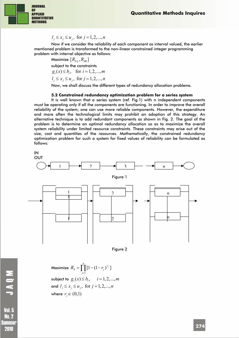
Quantitative Methods Inquires
274
j j jl x u≤ ≤ , for 1,2,...,j n=
Now if we consider the reliability of each component as interval valued, the earlier mentioned problem is transformed to the non-linear constrained integer programming problem with interval objective as follows:
Maximize [ , ]S SRLR R
subject to the constraints ( ) , for 1,2,...,i ig x b i m≤ =
j j jl x u≤ ≤ , for 1,2,...,j n=
Now, we shall discuss the different types of redundancy allocation problems. 5.2 Constrained redundancy optimization problem for a series system It is well known that a series system (ref. Fig.1) with n independent components
must be operating only if all the components are functioning. In order to improve the overall reliability of the system; one can use more reliable components. However, the expenditure and more often the technological limits may prohibit an adoption of this strategy. An alternative technique is to add redundant components as shown in Fig. 2. The goal of the problem is to determine an optimal redundancy allocation so as to maximize the overall system reliability under limited resource constraints. These constraints may arise out of the size, cost and quantities of the resources. Mathematically, the constrained redundancy optimization problem for such a system for fixed values of reliability can be formulated as follows:
IN OUT
Figure 1
Figure 2
Maximize 1
[1 (1 ) ]jn
xS j
j
R r=
= − −∏
subject to ( ) , 1,2,...,i ig x b i m≤ =
and j j jl x u≤ ≤ , for 1,2,...,j n=
where (0,1)jr ∈
1 2 3 n
12 n1 2 n
1 2 n

Quantitative Methods Inquires
275
Now if we consider component reliabilities as interval valued, i.e., [ , ]j jL jRr r r= then the above problem reduces to
Maximize 1
[ , ] [{1 (1 ) },{1 (1 ) }]j jn
x xSL SR jL jR
j
R R r r=
= − − − −∏
subject to ( ) , 1,2,...,i ig x b i m≤ =
and j j jl x u≤ ≤ , for 1,2,...,j n=
This is an INLP with interval valued objective. 5. 3. Hierarchical series-parallel system A reliability system is called a hierarchical series parallel system (HSP) if the system
can be viewed as a set of subsystems arranged in a series parallel; each subsystem has a similar configuration; subsystems of each subsystem have a similar configuration and so on. For example let us consider a HSP system ( 10, 2)n m= = shown in the Fig. 3. This system has a nonlinear and non separable structure and consists of nested parallel and series system. The system reliability of HSP is given by
3 1 2 4 5 6 7 8 9 10{1 1 [1 (1 )] (1 )}(1 )SR Q R R R R R Q Q Q R= − ⟨ − − − ⟩ − −
Mathematically, the constrained redundancy optimization problem for this system for fixed values of reliability can be formulated as follows:
Maximize 3 1 2 4 5 6 7 8 9 10{1 1 [1 (1 )] (1 )}(1 )SR Q R R R R R Q Q Q R= − ⟨ − − − ⟩ − −
subject to ( ) , 1,2,...,i ig x b i m≤ =
and j j jl x u≤ ≤ , for 1,2,...,j n=
where (0,1)jr ∈
Now if we consider the component reliabilities as interval valued, i.e., [ , ]j jL jRr r r= then the above problem reduces to the following form:
3 3 1 1 2 2 4 4 5 5 6 6
7 7 8 8 9 9 10 10
Maximize[ , ] {1 1 (1 [ , ](1 [ , ][ , ]))[ , ] (1 [ , ][ , ])}(1 [ , ][ , ][ , ])[ , ]
SL SR L R L R L R L R L R L R
L R L R L R L R
R R Q Q R R R R R R R R R RQ Q Q Q Q Q R R
= − ⟨ − − − ⟩ −−
subject to ( ) , 1,2,...,i ig x b i m≤ =
and j j jl x u≤ ≤ , for 1,2,...,j n=
This is an INLP with interval valued objective.
Figure 3
5 6
7 8
9
10 1 2
3 4

Quantitative Methods Inquires
276
5.4 Complex System When a reliability system can be reduced to series and parallel configurations,
there exist combinations of components which are connected neither in a series nor in parallel. Such systems are called complex or non parallel series systems. This system is also called the bridge system.
For example, let us consider a bridge system ( 5, 3)n m= = shown in Fig.4. This system consists of five subsystems and three nonlinear and non-separable constraints. The overall system reliability SR is given by the expression as follows:
5 1 3 2 4 5 1 2 3 4(1 )(1 ) [1 (1 )(1 )]SR R QQ Q Q Q R R R R= − − + − − − ,
where ( )j j jR R x= and 1j jQ R= − for all 1,...,5j = .
Mathematically, the constrained redundancy optimization problem for such complex system for fixed values of reliability can be formulated as follows:
Maximize 5 1 3 2 4 5 1 2 3 4(1 )(1 ) [1 (1 )(1 )]SR R QQ Q Q Q R R R R= − − + − − −
subject to ( ) , 1,2,...,i ig x b i m≤ =
and j j jl x u≤ ≤ , for 1,2,...,j n=
where (0,1)jr ∈
Since the overall system has a complex structure, the objective function is also non-linear and non-separable.
Now if we consider the component reliabilities as interval valued, i.e., [ , ]j jL jRr r r= then the above problem reduces to the following form as follows:
5 5 1 1 3 3 2 2 4 4
5 5 1 1 2 2 3 3 4 4
Maximize[ , ] [ , ](1 [ , ][ , ])(1 [ , ][ , ])[ , ]{1 (1 [ , ][ , ])(1 [ , ][ , ])}
SL SR L R L R L R L R L R
L R L R L R L R L R
R R R R Q Q Q Q Q Q Q QQ Q R R R R R R R R
= − −+ − − −
subject to ( ) , 1,2,...,i ig x b i m≤ =
and j j jl x u≤ ≤ , for 1,2,...,j n=
This is an INLP with interval valued objective.
Figure 4 5.5 -out-of- k n System A k out of n− − − system is an n -component system which functions when at
least k of its n components function. This redundant system is sometimes used in the place of pure parallel system. It is also referred to as :k out of n G− − − system. An n -
component series system is a :n out of n G− − − system whereas a parallel system with n -
components is a 1 :out of n G− − − system. When all of the components are independent
1 2
3 4
5

Quantitative Methods Inquires
277
and identical, the reliability of k out of n− − − system can be written
as (1 )n
j n jS
j k
nR r r
j−
=
⎛ ⎞= −⎜ ⎟
⎝ ⎠∑ , where r is the component reliability.
6. GA based constraint handling technique In the application of Genetic Algorithm for solving the reliability optimization
problems with interval objective[ 21-23], there arises an important question for handling the constraints relating to the problem. During the past, several approaches viz. penalty-based method, methods that preserve the feasibility of solutions, methods that clearly distinguish between feasible and unfeasible solutions and hybrid methods have been proposed to handle the constraints in evolutionary algorithms [16-19] for solving the problems with fixed objective [24]. Among these approaches, penalty-based technique is very well known and widely applicable. In this approach, constraints are added /subtracted to the objective function in different ways. To avoid the infeasible solution, the fitness function is increased /decreased with a penalty term multiplied by a so called penalty coefficient. However, there arises a difficulty to select the initial value and updating strategy for the penalty coefficient. To avoid this situation, Deb [24] proposed a GA based penalty technique called Parameter Free Penalty (PFP) technique replacing the objective function value of GA by worst objective value of feasible solution of previous generation and without multiplying the penalty coefficient. This means that the fitness function values of infeasible solution do not depend on the objective function value. As the mentioned constrained optimization problem is of interval valued, therefore the problem to be solved with a new fitness function is of the following interval form:
Maximize
1 1
ˆ ˆ[ ( ), ( )] [ ( ), ( )] [ max{0, ( ) }, max{0, ( ) }] ( )m m
SL SR SL SR i i i ii i
R x R x R x R x g x b g x b xθ= =
= − − − +∑ ∑ (1)
where [0,0] if
( )[ ( ), ( )] min[ , ] ifSL SR SL SR
x Sx
R x R x R R x Sθ
∈⎧= ⎨− + ∉⎩
and { : ( ) , 1,2,..., and }i iS x g x b i m l x u= ≤ = ≤ ≤
Here the parameter min[ , ]SL SRR R is the value of interval valued objective function
of the worst feasible solution in the population. Alternatively, the problem may be solved with another fitness function by penalizing a large positive number (say M which can be written in interval form as [ , ]M M ) [25]. We denote this penalty as Big-M penalty and its form is as follows:
Maximize ˆ ˆ[ ( ), ( )] [ ( ), ( )] ( )SL SR SL SRR x R x R x R x xθ= +
(2)
where [0,0] if
( )[ ( ), ( )] [ , ] ifSL SR
x Sx
R x R x M M x Sθ
∈⎧= ⎨− + − − ∉⎩
and { : ( ) , 1,2,..., and }i iS x g x b i m l x u= ≤ = ≤ ≤
The above problems (1) and (2) are non-linear unconstrained integer programming problem with interval coefficient.

Quantitative Methods Inquires
278
7. Solution procedure Now we have to solve the above nonlinear maximization problems (1) and (2) with
the help of GA. For this purpose, we have developed two types of GA with different fitness function based on PFP and Big-M penalty techniques. We call these GAs as PFP-GA and Big-M-GA respectively.
The different steps of this algorithm are described as follows: 7.1 Algorithm Step-1: Initialize the parameters of genetic algorithm, bounds of variables and
different parameters of the problem. Step-2: 0t = [ t represents the number of current generation]. Step-3: Initialize the chromosome of the population ( )P t [ ( )P t represents the
population at -t th generation]. Step-4: Evaluate the fitness function of each chromosome of ( )P t considering the
objective function of either (1) or (2) as fitness function. Step-5: Find the best chromosome from the population ( )P t . Step-6: t is increased by unity. Step-7: If the termination criterion is satisfied go to step-14, otherwise, go to next
step. Step-8: Select the population ( )P t from the population ( 1)P t − of earlier
generation by tournament selection process. Step-9: Alter the population ( )P t by crossover, mutation and elitism process.
Step-10: Evaluate the fitness function value of each chromosome of ( )P t .
Step-11: Find the best chromosome from ( )P t .
Step-12: Compare the best chromosome of ( )P t and ( 1)P t − and store better one. Step-13: Go to step-6 Step-14: Print the last found best chromosome (which is the solution of the
optimization problem). Step-15: End. For implementing the above GA in solving the problems (1) and (2) the following
basic components are to be considered. • GA Parameters • Chromosome representation • Initialization of population • Evaluation of fitness function • Selection process • Genetic operators (crossover, mutation and elitism) • Termination criteria 7.2 GA Parameters There are different parameters used in the genetic algorithm, viz. population size
(p_size), maximum number of generations (m_gen), crossover rate/probability of crossover (p_cross) and mutation rate/probability of mutation (p_mute). There is no hard and fast rule for choosing the population size for GA. However, if the population size is considered to be large, storing of the data in the intermediate steps of GA may create some difficulties at the time of computation with the help of computer. On the other hand, for very small population size, some genetic operations can not be implemented. Particularly, mutation operator does not work properly as the mutation rate is very low. Regarding the maximum number of generations, there is no indication for considering this value. Generally, it is problem

Quantitative Methods Inquires
279
dependent on problem to problem. Particularly, it depends upon the number of genes (variables) of a chromosome (solution) in artificial genetics. Again, from the natural genetics, it is obvious that the crossover rate is always greater than that of mutation rate. Usually, the crossover rate varies from 0.8 to 0.95 whereas the mutation rate varies from 0.05 to 0.2. Sometimes, it is considered as 1 nwhere n be the number of genes (variables) of the chromosomes (solutions).
7.3 Chromosome representation and initialization In the applications of GA, the appropriate chromosome (individual) representation
of solution for the given problems is an important task to the users. There are different types of representations, viz. binary, real, octal, hexadecimal coding, available in the existing literature. Among these representations, real coding representation is very popular as this type of chromosome representation looks like a vector. In this representation, each component (gene) of the chromosome is the values of decision variables of the optimization problems which are to be solved by GA.
7.4 Initialization of population After the selection of chromosome representation, the next step is to initialize the
chromosomes that will take part in the artificial genetic operations like natural genetics. This procedure produces population size number of chromosomes in which every component for each chromosome is randomly generated within the bounds of the corresponding decision variable. There are different procedures for selecting a random number for each component of the chromosomes. Here for each component of the chromosome, a random value is selected from the discrete set of values within its bounds.
7.5 Evaluation of fitness function After getting a population of potential solutions, we need to check how good they
are. So we have to calculate the fitness value for each chromosome. In this evaluation, the value of objective function corresponding to the chromosome is taken as the fitness value of that chromosome. Here, the transformed unconstrained objective function due to different penalty technique is considered as the fitness function.
7.6 Selection In artificial genetics, the selection operator plays an important role. Usually, it is the
first operator applied to the population. The primary objective of this operator is to emphasize on the above average solutions and eliminate below average solutions from the population for the next generation under the well-known evolutionary principle “survival of the fittest”. In this work, we have used tournament selection scheme of size two with replacement as the selection operator. This operator selects the better chromosome/individual from randomly selected two chromosomes/individuals. This selection procedure is based on the following assumptions:
(i) When both the chromosomes / individuals are feasible then the one with better fitness value is selected.
(ii) When one chromosome/individual is feasible and another is infeasible then the feasible one is selected.
(iii) When both the chromosomes/individuals are infeasible with unequal constraint violations, then the chromosome with less constraint violation is selected.
(iv) When both the chromosomes/individuals are infeasible with equal constraint violations, then any one chromosome/individual is selected.
7.7 Crossover After the selection process, other genetic operators like crossover and mutation are
applied to the resulting chromosomes (those which have survived). Crossover is an operation that really empowers the GA. It operates on two or more parent solutions at a time and

Quantitative Methods Inquires
280
generates offspring by recombining the feature of the parent solutions. In this operation,
expected [ ]p_cross*p_size (* denotes the product and [ ] denotes the integral value)
number of chromosomes will take part. Hence in order to perform the crossover operation,
select [ ]p_cross*p_size numbers of chromosomes are selected. In our work, the operation
is done in the following manner. Step-1: Find the integral value of p_cross*p_size and store it inN .
Step-2: Select the chromosomes kv and iv randomly from the population for
crossover. Step-3: The components kjv′ and ijv′ ( 1,2,..., )j n= of two offspring will be created
by either kj kjv v g′ = − and ij ijv v g′ = + if kj ijv v>
Or, kj kjv v g′ = + and ij ijv v g′ = − , where g is a random integer number between
0 and kj ijv v− .
Step-4: Repeat step-2 and step-3 for 2
Ntimes.
7.8 Mutation The aim of mutation operation is to introduce the random variations into the
population. Sometimes, it helps to regain the information lost in earlier generations. Mainly, this operator is responsible for fine tuning capabilities of the system. This operator is applied to a single chromosome only. Usually, its rate is very low; otherwise it would defeat the order building generated through selection and crossover operations. Mutation attempts to bump the population gently into a slightly better way, i.e., the mutation changes single or all the genes of a randomly selected chromosome slightly. In this work, we have used uniform mutation. If the gene ikv of chromosome iv is selected for mutation and domain of
ikv is[ , ]ik ikl u , then the reduced value of ikv is given by
( ), if random digit is 0.
( ), if random digit is1.
ik ik ikik
ik ik ik
v u vv
v v l
+ Δ −′ =
− Δ −
⎧⎨⎩
where {1,2,..., }k n∈ and ( )yΔ returns a value in the range[0, ]y . In our work, we have taken
( )yΔ = A random integer between[0, ]y . 7.9 Elitism Sometimes, in any generation, there is a chance that the best chromosome may be
lost when a new population is created by crossover and mutation operations. To remove this situation the worst individual/chromosome is replaced by that best individual/chromosome in the current generation. Instead of single chromosome one or more chromosomes may take part in this operation. This process is called as elitism.
7.10 Termination criteria The termination condition is to stop the algorithm when either of the following
three conditions is satisfied: (i) the best individual does not improve over specified generations. (ii) the total improvement of the last certain number of best solutions is less than a
pre-assigned small positive number or (iii) The number of generations reaches maximum number of generation i.e.,
max_gen.

Quantitative Methods Inquires
281
In this work we have used first condition and we take 10 generations as a specified generation.
8. Numerical Examples
To illustrate the proposed GAs (viz. PFP-GA and Big-M-GA) for solving constrained
redundancy allocation problems with interval valued reliabilities of components, we have solved four numerical examples. It is to be noted that for solving the said problem with fixed valued reliabilities of components, the reliability of each component are taken as interval with the same lower and upper bounds of interval. In first three examples, the reliabilities of the components are interval valued whereas in the last example (taken from Ha and Kuo [12]), it is fixed. For each example, 20 independent runs have been performed by both the GAs, of which the following measurements have been collected to compare the performance of PFP-GA and Big-M-GA.
(i) Best found system reliability (ii) Average generations (iii) Average CPU times The proposed Genetic Algorithms are coded in C programming language and run
in Linux environment. The computation work has been done on the PC which has Intel core-2 duo processor with 2 GHz. In this computation, different population size has been taken for different problems. However, the crossover and mutation rates are taken as 0.95 and 0.15 respectively.
Example-8.1 (Ref. section 5.2)
Maximize 5
1
[ , ] [{1 (1 ) },{1 (1 ) }]j jx xSL SR jL jR
j
R R r r=
= − − − −∏
subject to 5
2
1
5
1
5
1
0,
[ exp( ) 0,4
exp( ) 0,4
j jj
jj j
j
jj j
j
p x P
xc x C
xw x W
=
=
=
− ≤
+ − ≤
− ≤
∑
∑
∑
Table 1: Parameter used in Example -8.1
j rj pj P cj C wj W
1 [0.76,0.83] 1 7 7 2 [0.82,0.87] 2 110 7 175 8 200 3 [0.88,0.93] 3 5 8 4 [0.61,0.67] 4 9 6 5 [0.70,0.80] 2 4 9
Example-8.2 (Ref. section 5.3)
3 3 1 1 2 2 4 4 5 5 6 6
7 7 8 8 9 9 10 10
Maximize[ , ] {1 1 (1 [ , ](1 [ , ][ , ]))[ , ] (1 [ , ][ , ])}(1 [ , ][ , ][ , ])[ , ]
SL SR L R L R L R L R L R L R
L R L R L R L R
R R Q Q R R R R R R R R R RQ Q Q Q Q Q R R
= − ⟨ − − − ⟩ −−
subject to

Quantitative Methods Inquires
282
2 33 5 1011 2 2 3 4 4 5 5 6 7 6 8 7 9
2 33 4 6 9 101 1 2 2 3 5 4 7 8 5 9 6 2
exp( ) exp( ) [ exp( )] exp( ) 120 0,2 2 4 2
exp( ) exp( ) [ exp( )] exp( ) 130 0,2 4 2 4
x x xxc x c c x c x c x x c x c x
x x x x xw x x w w x w x x w x w x
+ + + + + + + − ≤
+ + + + + + − ≤
Table 2: Parameter used in Example-8.2
j 1 2 3 4 5 6 7 8 9 10
jr [.80,.84] [.87,.90] [.89,.93] [.84,.86] [.88,.90] [.9,.95] [.8,.85] [.91,.95] [.8,.83] [.88,.92]
jc 8 4 2 2 1 6 2 8 - -
jw 16 6 7 12 7 1 9 - - -
jl 1 1 1 1 1 1 1 1 1 1
ju 4 5 6 7 5 5 3 3 4 6
Example-8.3 (Ref. section 5.4)
5 5 1 1 3 3 2 2 4 4
5 5 1 1 2 2 3 3 4 4
Maximize[ , ] [ , ](1 [ , ][ , ])(1 [ , ][ , ])[ , ]{1 (1 [ , ][ , ])(1 [ , ][ , ])}
SL SR L R L R L R L R L R
L R L R L R L R L R
R R R R Q Q Q Q Q Q Q QQ Q R R R R R R R R
= − −+ − − −
subject to
212 3 4 5
3 2 51 42 3 4
2 2 332 2 3 1 4 5
1 2 3 4 5
10exp( ) 20 3 8 200 0,2
10exp( ) 4exp( ) 2 6[ exp( )] 7exp( ) 310 0,2 4 4
12[ exp( )] 5 exp( ) 3 2 520 0,4
(1,1,1,1,1) ( , , , , ) (6,3,5,6,6),
x x x x x
xx xx x x
xx x x x x x
x x x x x
+ + + − ≤
+ + + + + − ≤
+ + + + − ≤
≤ ≤
where
1 1( ) {[0.78,0.82],[0.83,0.88],[0.89,0.91],[0.915,0.935],[0.94,0.96],[0.965,0.985]}; R x =
2
2 2( ) 1 (1 [0.73,0.77]) ;
xR x = − −
33
13 1
3 32
1( ) ([0.87,0.89]) ([0.11,0.13]) ;
xx kk
k
xR x
k
++ −
=
+⎛ ⎞= ⎜ ⎟
⎝ ⎠∑
44 4( ) 1 (1 [0.68,0.72]) ;
xR x = − −
55 5( ) 1 (1 [0.83,0.86]) ;
xR x = − −

Quantitative Methods Inquires
283
Example-8.4 (Ref. section 5.4)
5 5 1 1 3 3 2 2 4 4
5 5 1 1 2 2 3 3 4 4
Maximize[ , ] [ , ](1 [ , ][ , ])(1 [ , ][ , ])[ , ]{1 (1 [ , ][ , ])(1 [ , ][ , ])}
SL SR L R L R L R L R L R
L R L R L R L R L R
R R R R Q Q Q Q Q Q Q QQ Q R R R R R R R R
= − −+ − − −
subject to
212 3 4 5
3 2 51 42 3 4
2 2 332 2 3 1 4 5
1 2 3 4 5
10exp( ) 20 3 8 200 0,2
10exp( ) 4exp( ) 2 6[ exp( )] 7 exp( ) 310 0,2 4 4
12[ exp( )] 5 exp( ) 3 2 520 0,4
(1,1,1,1,1) ( , , , , ) (6,3,5,6,6), x n
x x x x x
xx xx x x
xx x x x x x
x x x x x +
+ + + − ≤
+ + + + + − ≤
+ + + + − ≤
≤ ≤ ∈
where
1 1( ) {[.8,.8],[.85,.85],[.9,.9],[.925,.925],[.95,.95],[.975,.975]};R x = 2
2 2( ) 1 (1 [0.75,0.75]) ;xR x = − −
33
13 1
3 32
1( ) ([0.88,0.88]) ([0.12,0.12]) ;
xx kk
k
xR x
k
++ −
=
+⎛ ⎞= ⎜ ⎟
⎝ ⎠∑
44 4( ) 1 (1 [0.7,0.7]) ;xR x = − −
55 5( ) 1 (1 [0.85,0.85]) ;
xR x = − −
Table 3: Numerical results for Example 8.1-8.4
Meth
od
Example X
Best found system
reliability sR Average CPU
time (sec.) Average
Generation Population
Size
8.1
(3,2,2,3,3)
[0.860808,0.930985]
0.0001
12.10
50
8.2 (1,2,2,5,4,4,2,2,1,5
) [0.999909,0.999987] 0.0105 17.55 100
8.3 (5,1,2,4,4) [0.991225,0.999872] 0.0200 11.20 200 PFP
-GA
8.4 (3,2,4,4,2) [0.999382,0.999382] 0.0100 12.40 100
8.1
(3,2,2,3,3)
[0.860808,0.930985]
0.0001
12.80
50
8.2 (1,2,2,5,4,4,2,2,1,5
) [0.999909,0.999987] 0.0110 17.75 100
8.3 (5,1,2,4,4) [0.991225,0.999872] 0.0200 10.90 200 Big
-M-G
A
8.4 (3,2,4,4,2) [0.999382,0.999382] 0.0100 12.55 100
9. Sensitivity Analysis To study the performance of our proposed GAs like PFP-GA and Big-M-GA based
on two different types of penalty techniques, sensitivity analyses have been carried out graphically on the centre of the interval valued system reliability with respect to GA parameters like, population size, crossover and mutation rate separately keeping the other parameters at their original values. These are shown in Fig.5-Fig.7.
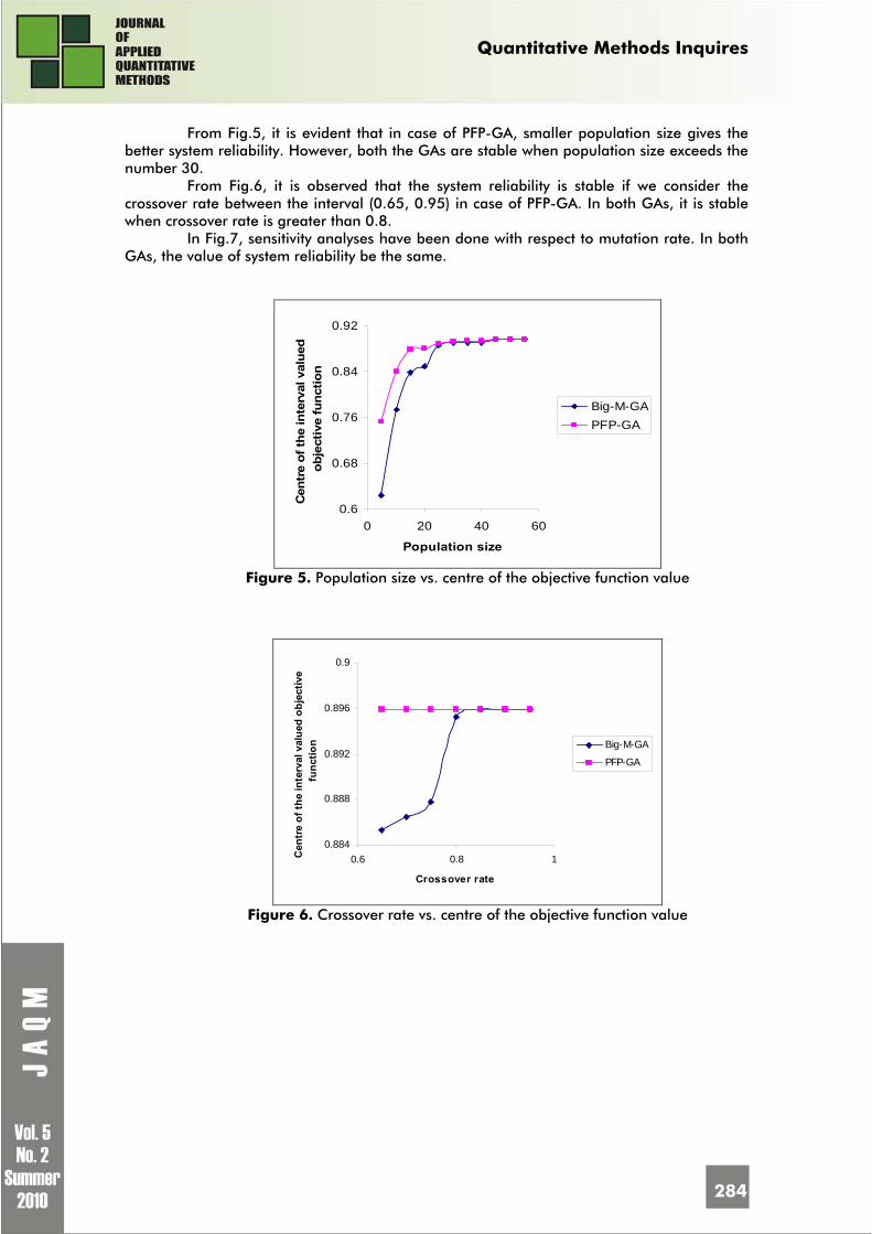
Quantitative Methods Inquires
284
From Fig.5, it is evident that in case of PFP-GA, smaller population size gives the better system reliability. However, both the GAs are stable when population size exceeds the number 30.
From Fig.6, it is observed that the system reliability is stable if we consider the crossover rate between the interval (0.65, 0.95) in case of PFP-GA. In both GAs, it is stable when crossover rate is greater than 0.8.
In Fig.7, sensitivity analyses have been done with respect to mutation rate. In both GAs, the value of system reliability be the same.
0.6
0.68
0.76
0.84
0.92
0 20 40 60
Population size
Cen
tre
of th
e in
terv
al v
alue
d ob
ject
ive
func
tion
Big-M-GAPFP-GA
Figure 5. Population size vs. centre of the objective function value
0.884
0.888
0.892
0.896
0.9
0.6 0.8 1
Crossover rate
Cen
tre
of th
e in
terv
al v
alue
d ob
ject
ive
func
tion Big-M-GA
PFP-GA
Figure 6. Crossover rate vs. centre of the objective function value

Quantitative Methods Inquires
285
0.5
0.75
1
0 0.05 0.1 0.15 0.2 0.25
Mutation rate
Cen
tre
of th
e in
terv
al v
alue
d ob
ject
ive
func
tion
Big-M-GA
PFP-GA
Figure 7. Mutation rate vs. centre of the objective function value
10. Conclusions
In this paper, reliability redundancy allocation problems of series-parallel/parallel-
series/complex system with some resource constraints have been solved. In those systems, reliability of each component has been considered as imprecise number and this imprecise number has been represented by an interval number which is more appropriate representation among other representations like, random variable representation with known probability distribution, fuzzy set with known fuzzy membership function or fuzzy number. For handling of resource constraints, the corresponding problem has been converted into unconstrained optimization problem with the help of two different parameter free penalty techniques. Therefore, the transformed problem is of unconstrained interval valued optimization problem with integer variables. To solve the transformed problem, we have developed real coded GA for integer variables with interval valued fitness function, tournament selection, uniform crossover, uniform mutation and elitism of size one. In tournament selection and elitism operation, recently developed definitions of interval ranking have been used. In the existing penalty function technique, tuning of penalty parameter is a formidable task. From the performance of GAs, it is observed that both the GAs with both fitness function due to different penalty techniques take very lesser CPU time with very small generations to solve the problems. It is clear from the expression of the system reliability, that the system reliability is a monotonically increasing function with respect to the individual reliabilities of the components. Therefore, there is one optimum setup irrespective of the choice of the upper bound or lower bound of the component reliabilities. As a result, the optimum setup obtained from the upper bound/lower bound will provide both the upper bound and the lower bound of the optimum system reliability. However, the interval approach presented in this paper has a wider applicability. For future research, one may use the proposed GAs in solving other reliability optimization problems like Chance- constrained reliability optimization problems, Network reliability optimization problems, etc.
References
1. Kuo, W., Prasad, V. R., Tillman, F. A. and Hwuang, C. L. Optimal Reliability Design
Fundamentals and application, Cambridge University Press, 2001 2. Ghare, P. M. and Taylor, R. E. Optimal redundancy for reliability in series system,
Operations Research 17, 1969, pp. 838-847

Quantitative Methods Inquires
286
3. Tillman, F. A., Hwuang, C. L. and Kuo, W. Optimization technique for system reliability with redundancy: A Review. IEEE Trans. Reliability 26, 1977, pp.148-155
4. Nakagawa, Y., Nakashima, K. and Hattori, Y. Optimal reliability allocation by branch-and -bounded technique. IEEE Trans. Reliability, 27, 1978, pp.31-38
5. Tzafestas, S. G. Optimization of system reliability: A survey of problems and techniques, International Journal of System Science, 11, 1980, pp.455-486
6. Shantikumar, J. G. and Yao, D. D. On server allocation in multiple centre manufacturing systems, Operations Research 36, 1988, pp. 333-341
7. Misra, K.B. and Sharama, U. An efficient algorithm to solve integer-programming problems arising in system reliability design. IEEE Trans. Reliability 40, 1991, pp. 81-91
8. Sundarajan C. Guide to Reliability Engineering: Data, Analysis, Applications, Implementation, and Management, New York: Van Nostrand Reinhold, 1991
9. Chern, M.S. On the computational complexity of reliability redundancy allocation in a series system, Operations Research Letter 11, 1992, pp. 309-315
10. Ohtagaki, H., Nakagawa, Y., Iwasaki, A. and Narihisa, H. Smart greedy procedure for solving a nonlinear knapsacclass of reliability optimization problems, Mathl. Comput. Modeling 22, 1995, pp.261-272
11. Sun Xiaoling and Li Duan. Optimal Condition and Branch and Bound Algorithm for Constrained Redundancy Optimization in Series System, Optimization and Engineering, 3, 2002, pp. 53-65
12. Ha, C. and Kuo, W. Reliability redundancy allocation: An improved realization for nonconvex nonlinear programming problems, European Journal of Operational Research, 171, 2006, pp. 124-138
13. Gen, M. and Yun, Y. Soft computing approach for reliability optimization, Reliability Engineering & System Safety, 91, 2006, pp.1008-1026
14. Kuo, W., Prasad, V. R., Tillman, F. A. and Hwuang, C. L. Optimal Reliability Design Fundamentals and application, Cambridge University Press, 2001
15. Mahato, S. K. and Bhunia, A. K. Interval-Arithmetic-Oriented Interval Computing Technique for Global Optimization, Applied Mathematics Research eXpress, 2006, pp.1-19
16. Goldberg, D. E. Genetic Algorithms: Search, Optimization and Machine Learning, Reading, MA. Addison Wesley, 1989
17. Michalawich, Z. Genetic Algorithms + Data structure = Evaluation Programs, Berlin: Springer Verlag, 1996
18. Gen, M. and Cheng, R. Genetic algorithms and engineering optimization, John Wiley & Sons inc., 2000
19. Sakawa, M. Genetic Algorithms and fuzzy multiobjective optimization, Kiuwer Academic Publishers, 2002
20. Hansen, E. and Walster G. W. Global optimization using interval analysis, New York: Marcel Dekker Inc., 2004
21. Ishibuchi, H. and Tanaka, H. Multiobjective programming in optimization of the interval objective function, European Journal of Operational Research 48, 1990, pp.219-225
22. Chanas, S. and Kuchta, D. Multiobjective programming in the optimization of interval objective functions-A generalized approach, European journal of Operational Research, 94, 1996, pp.594-598
23. Sengupta, A. and Pal, T. K. Theory and methodology on comparing interval numbers, European Journal of Operational Research,127, 2007, pp.28-43
24. Deb, K. An efficient constraint handling method for genetic algorithms, Computer Methods in Applied Mechanics and Engineering, 186, 2000, pp.311-338
25. Gupta, R. K., Bhunia, A. K. and Roy, D. A GA based penalty function technique for solving constrained redundancy allocation problem of series system

Quantitative Methods Inquires
287
with interval valued reliability of components, Journal of Computational and Applied Mathematics232, 2009, pp. 275-284
1 Acknowledgements The second author would like to acknowledge the support of Defence Research Development Organization (DRDO), India, for conducting this work.

Quantitative Methods Inquires
288
MULTINOMIAL LOGISTIC REGRESSION: USAGE AND APPLICATION IN RISK ANALYSIS
Anass BAYAGA School of Initial Teacher Education (SITE), Faculty of Education, University of Fort Hare, South Africa E-mail: [email protected]
Abstract: The objective of the article was to explore the usage of multinomial logistic regression (MLR) in risk analysis. In this regard, performing MLR on risk analysis data corrected for the non-linear nature of binary response and did address the violation of equal variance and normality assumptions. Additionally, use of maximum likelihood (-2log) estimation provided a means of working with binary response data. The relationship of independent and dependent variables was also addressed. The data used included a cohort of hundred risk analyst of a historically black South African University. In this analysis, the findings revealed that the probability of the model chi-square (17.142) was 0.005, less than the level of significance of 0.05 (i.e. p<0.05). Suggesting that there was a statistically significant relationship between the independent variable-risk planning (Rp) and the dependent variable-control mechanism (control mecs) (p<0.05). Also, there was a statistically significant relationship between key risks assigned (KSA) and time spent on risk mitigation. For each unit increase in confidence in control mecs, the odds of being in the group of survey respondents who thought institution spend too little time on Rp decreased by 74.7%. Moreover, the findings revealed that survey respondents who had less confidence in control mecs were less likely to be in the group of survey respondents who thought institution spent about the right amount of time on risk planning.
Key words: Binary variable; Log odds ratio; Logistic regression model; (log) Likelihood ratio statistic; -2 Log Q; Wald statistic; Model fit; -2 Log L. Quantitative risk analysis
1. Context of study Modeling of risk processes such as risk awareness, risk identification, monitoring
and reporting, planning and mitigation etc is among rather difficult subjects tackled by risk analyst especially in applying multinomial logistic regression in dynamic (social) setting. Invariably though, social science research (Yu, Lai & Wang, 2008; Fan & Xiao, 2006) problems somewhat call for analysis and prediction of a dichotomous1 outcomes. Traditionally, such research outcomes were addressed by either ordinary least squares (OLS) regression or linear discriminant function analysis (Hosmer & Lemeshow, 2000). However, both techniques, as a result of their nature, depend on strict statistical assumptions, thus, normality of independent variables, linearity of relationships, multicollinearity among independent variables, equal dispersion matrices for discriminant analysis (Tabachnick et al., 2001). These assumptions which are not easily observed in a dynamic setting are part of multiple2 regression.
Introduction of multinomial logistic regression was an alternative regression analysis to cater for conditions that do not necessarily obey the assumptions listed above with the exception of multicollinearity (Hosmer & Lemeshow, 2000). In the last decade, the technique, like other univariate and multivariate data analysis methods, started to find a

Quantitative Methods Inquires
289
prominent place in the medicine, engineering and the manufacturing industries. This development led researchers in risk analysis to build more accurate and useful statistical models by applying it in risk analysis (Liebenberg & Hoyt, 2003; Hosmer & Lemeshow, 2000). Meanwhile, despite being in use in general statistical analysis for many years, it has received rather little attention in the risk analysis literature compared to other regression applications regarding modelling of explanatory and response variable (Liebenberg & Hoyt, 2003;Hosmer & Lemeshow, 2000).
Recent studies (Crane, Gibbons, Jolley, Van Belle, 2007; Hedeker, 2003; Menard, 2002; Tabachnick, Fidell & Osterlind, 2001; Harrell, 2001; Hosmer & Lemeshow, 2000) have noted that modelling relationship between explanatory (predictor) and response variables is a fundamental activity encountered in risk analysis. The accounts of these studies suggest that simple linear regression is often used to investigate the relationship between a single predictor variable and a single response (dependent) variable. But, when there are several explanatory variables though, multinomial logistic regression is used.
However, often the response (dependent variable) as some of the authors argued (Menard, 2002; Tabachnick et al., 2001; Harrell, 2001; Hosmer & Lemeshow, 2000) is not a numerical value. Instead, the response is simply a designation of one of two possible outcomes (a binary response); example, alive or dead, success or failure, yes or no. Data involving relationship between explanatory variables and binary responses proliferate in just about every discipline from engineering to the natural sciences, to medicine etc. Invariably though, what remains a matter of concern for many practitioners and theorists of risk analysis in University is the questions of how to model relationship between explanatory variables and a binary response variable (Liebenberg & Hoyt, 2003; Tabachnick et al., 2001; Harrell, 2001; Hosmer & Lemeshow, 2000).
Scholars (Hamilton, 2003; Hendrickx, 2000; McCullagh, 1980) have argued that the difficulty for both practitioners and theorists in modeling of risk processes steams from the social setting within which risk parameters are applied. Additionally, the authors suggested that little scholarly literature has delved into application of multinomial logistic regression in analysis of risks parameters particularly in a University context.
Whiles, there remain little studies being conducted in risk analysis with regards to MLR in the context of a University, many recent studies (Van Gelderen, Thurik & Bosma, 2006; Jalilvand & Switzer, 2005; McNeil, Frey & Embrechts, 2005; Mishra & El-Osta, 2002) have encouraged its usage due to its relevance to the field of risk analysis. Following the above, the paper explored the application of multinomial logistic regression via University-wide risk analysis. It does this by using concepts from simple and multiple linear regressions which are carried over to MLR. Additionally, ideas of maximum likelihood estimation are central to the modelling of the MLR data.
1.1. Multinomial Logistic Regression The multinomial (polytomous) logistic regression model is a simple extension of the
binomial logistic regression model. It is used when the dependent variable has more than two nominal or unordered categories, in which dummy coding3 of independent variables is quite common. In using multinomial logistic regression in risk analysis, the dependent (response) variable is dummy coded into multiple 1/0 variables (cf. sections 3 for details). This means that there is a variable for all categories but one, so if there are M categories, there will be M-1 dummy variables. All but one category has its own dummy variable. Each category’s dummy variable has a value of 1 for its category and a 0 for all others. One category, the reference category, does not need its own dummy variable, as it is uniquely identified by all the other variables being 0. With regards to the above, risk analyst using multinomial logistic regression can then estimate a separate binary logistic regression model for each of those dummy variables. The result is M-1 binary logistic regression models. The most significant factor to consider here is that each one tells the effect of the predictors of risk on the probability of success in that category, in comparison to the reference category. Noting though that each model has its own intercept and regression coefficients- the reason being that predictors of risk analysis processes could affect each category differently (cf. sections 2 & 3 for details).

Quantitative Methods Inquires
290
1.2. Why Multinomial Logistic Regression instead of other Techniques? Most of multivariate analysis techniques require the basic assumptions of normality
and continuous data, involving independent and/or dependent variables as aforementioned. This necessity manifests itself also in the application of MLR data collection and measurement steps in risk analysis, but to varying degree. Thus, whereas much stronger interval and ratio scales provide a good basis for a more comprehensive multivariate analysis, commonly used risk measurement scales such as five-point likert, ordinal, and nominal scales are usually considered unsuitable for multivariate analysis techniques, due to various assumption as listed above. For this reason, multinomial logistic regression was used where the above assumptions tend to be violated. This is evident in one main way in MLR analysis. Thus, it has alternative data distribution assumptions, suggesting that it generates more appropriate and correct findings in terms of model fit and correctness of the analysis regardless of any assumption (cf. section 3.1 for details).
A multinomial logistic regression model is a form of regression where the outcome variable (risk factor-dependent variable) is binary or dichotomous and the independents are continuous variables, categorical variables, or both. The application of multinomial logistic regression in risk analysis arises when an analyst analyses relationships between a non-metric dependent variable and metric or dichotomous independent variables. It compares multiple groups of risk processes such as risk mitigation, planning, monitoring identification, through a combination of binary logistic regressions (cf. section 3). The comparisons are equivalent to the comparisons for a dummy-coded dependent variable, with the group with the highest numeric score used as the reference group. Additionally, it provides a set of coefficients for each of the two comparisons. Multinomial logistic regression exists to handle the case of dependents with more classes. This is referred to as the multivariate case.
Thus, it is expected that multinomial logistic regression approach would do better when there is evidence of substantial departures from multivariate normality as is the case where there are some dichotomous or zero/one variables or where distributions are highly skewed or heavy-tailed especially in dynamic settings. In MLR however, hypotheses on significance of explanatory variables cannot be tested in quite the same way as say linear regression. Recall that in linear regression, where the response variables are normally distributed, one can use t- or F-test statistics for testing significance of explanatory variables. But in logistic regression, the response variables are Bernoulli distributed4, meaning that a risk analyst has to use different test statistics, which exact distributions are unknown. In this paper though, the researcher would not go into any technical details about test statistics, but focus on interpreting the results of a MLR analysis (cf. methodology, results and discussion of results). To this effect, two different types of test statistics, the (log) likelihood ratio statistic (often referred to as the -2log or deviance) and the Wald statistic would be used. The model is written somewhat differently in some software (cf. SPSS & SAS) than usual mathematical approach. In some software (cf. SAS), the sign is a plus, suggesting that increases in predictor values leads to an increase of probability in the lower-numbered response categories. The converse is true for software such as SPSS with a minus sign between the intercept and all the regression coefficients (cf. section 3 for details).This is a convention ensuring that for positive beta coefficients, increases in predictor values leads to an increase of probability in the higher-numbered response categories. It is recommended risk analyst make sure they understand how the model is set up in any statistical package before interpreting results. In general, the likelihood statistic is superior to the Wald statistic (in the sense that it gives more reliable results), so the paper would mainly concentrate on the likelihood ratio statistic (the reason for considering the Wald statistic too, is that it is computationally easy and is given automatically in the output of most statistical computer packages.
Tabachnick et al. (2001) argued that multinomial logistic regression technique has number of major advantages as a summary to the discussion above: (1) it is more robust to violations of assumptions of multivariate normality and equal variance-covariance matrices across groups; and (2) it is similar to linear regression, but more easily interpretable diagnostic statistics. Further, advantages of the analysis that raise its popularity come from

Quantitative Methods Inquires
291
the following assumptions: (3) most importantly, MLR does not assume a linear relationship between the dependent and independent variables; (4) independent variables need not to be interval (5) MLR does not require that the independents be unbounded and lastly (6) normally distributed error terms are not assumed.
Widely use of MLR as a problem solving tool, particularly in the fields of medicine, psychology, mathematical finance and engineering are as a result of the above advantages listed. This listed relevance attracted the present author’s attention in the case for University-wide risk analysis. Standing on the advantages, the purpose and extent of the usage of MLR in risk analysis research deserves a well-prepared review and application of the method (cf. sections 2 & 3). Such an application would provide valuable clues for future University-wide risk analyst about the scope of MLR, what would be expected from it, and how it would work in various risk problems. Following the above contestations and underlying advantages of MLR in risk analysis, the intent of this paper are as seen below (cf. 1.3).
1.3. Research Objectives The aims of the paper are to: a) Demonstrate the use of multinomial logistic regression in risk analysis b) Evaluate the use of maximum likelihood methods to perform multinomial
logistic regression in risk analysis. c) Demonstrate how to assess the fit of a multinomial logistic regression model
in risk analysis with the presence of independent variables. d) Determine the significance of explanatory variables. Following third research aim, the hypothesis posed is: Ho = there is no difference between model without independent variables (WINV)
and the model with independent variables (INV) Ha = there is a difference between model without independent variables and the
model with independent variables.
2. Method The study was undertaken in a historically black South African University in the
greater Eastern Cape Province. The University has a high but relatively heterogonous population density of risk analyst in various committees mandated to risk manage the university. This means that the University is equipped with various (academic, finance, human resource, information systems/infrastructure) directors and or managers who are largely in the knowledge of risk analysis. Historically, the risk/quality unit in University is the overseer of risks and quality checks of the University, which is headed by a director. The population for this study was hundred (100) risk analysts in various committees which were stratified. Information was collected from respondents with the aid of a structured and validated interview schedule, consisting of closed ended questions, based on the objectives/questions of the study. Data analysis was with the aid of both descriptive and inferential analysis (cf. section 3). Independent variables for this study were variables of risk analysis, in this case grouped into two (i) institutional risk planning and (ii) institutional risk mitigation. The dependent variable was characteristics of risk variables, which was measured in terms of six elements, viz (i) institution embedded risk management into its planning and operational processes to a sufficient extent (ii) institutional policy documents deal with risk management issues; iinternal auditors conduct audits as part of statutory regulation (iii) institution has control mechanisms to mitigate risk (iv) responsibility for the oversight of individual key risks are assigned to appropriate managers (v) the institution’s overall approach to risk management, as assessed for one-academic year is adequate for its strategic objectives (vi) the issues arising from audits are brought to the attention of the executive management team as appropriate. Since the independent variable was ordinal, the following cautions were considered, thus assumptions. Firstly, MLRA does not make any assumptions of normality, linearity, and homogeneity of variance for the independent variables (cf. sections 1.1 & 1.3). Secondly, because it does not impose these requirements, it

Quantitative Methods Inquires
292
is preferred to other class of analysis (e.g discriminant analysis) when the data does not satisfy these assumption
The overall test of relationship among the independent variables and groups defined by the dependent was based on the reduction in the likelihood values for a model which does not contain any independent variables and the model that contains the independent variables (cf. sections 3.1 & 3.2). This difference in likelihood followed a chi-square distribution x2, and was referred to as the model chi-square (cf. section 3). The significance test for the final model chi-square was the researcher’s statistical evidence of the presence of a relationship between dependent and independent variables (cf. section 3).
3. Results: Description of the data
This section describes results of the study. This included the description of the data.
Firstly, consideration was given to overall test of relationship, this described the overall test of relationship. Secondly, strength of MLR relationship was tested, this was done to establish the strength of MLR relationship. Thirdly, evaluating for the usefulness of logistic model and relationship between the independent and dependent variables.
3.1. Overall test of Relationship The first thing in MLR for any risk analyst is to describe the overall test of
relationship, in this case a relationship between the dependent and independent variables (cf. section 2-method). The presence of a relationship between the dependent and combination of independent variables is based on the statistical significance of the final model chi-square in the table 1; termed model fitting information. In this analysis, the distribution reveals that the probability of the model chi-square (17.142) was 0.005, less than the level of significance of 0.05 (i.e. p<0.05). The null hypothesis that there was no difference between the model without independent variables and the model with independent variables was rejected (cf. section 1.4). As evidenced in table 3.1 this suggested that the existence of a relationship between the independent variables and the dependent variable was supported, hence accepting the alternate (Ha) hypothesis.
Table 3.1. Model fitting information Model -2logLikelihood Chi-Square df Sig Intercept Only 272.024 . . . Final 225.334 17.142 6 .005
3.2. Strength of Multinomial Logistic Regression Relationship Once the relationship is established, the next important thing to do is to establish
the strength of multinomial logistic regression relationship. While, MLR does compute correlation measures to estimate the strength of the relationship (pseudo R square measures, such as Nagelkerke's R²), these correlation measures do not really tell an analyst much about the accuracy or errors associated with the model. A more useful measure to assess the utility of a multinomial logistic regression model was classification accuracy, which compares predicted group membership based on the logistic model to the actual, known group membership, which is the value for the dependent variable (cf. section 3.2.1). To assess the strength of multinomial logistic regression relationship, however, the evaluation of the usefulness for logistic models was considered (cf. sections 3.2.1. & 3.2.2).
In this case, using Cox & Snell R Square and the Nagelkerke R square value, they provide an indication of the amount of variation in the dependent variable. These are described as pseudo R square. The distribution in table 3.2 below reveals that the values are 0.181 and 0.322 respectively, suggesting that between 18.1% percent and 32.2% percent of the variability is explained by this set of variables used in the model.

Quantitative Methods Inquires
293
Table 3.2. Pseudo R-Square Step Cox &Snell R² NagelKerke R² .181 .322
3.2.1. Evaluating Usefulness for Logistic Models The proportional by chance accuracy rate was computed by calculating the
proportion of cases for each group based on the number of cases in each group in and then squaring and summing the proportion of cases in each group (0.371² + 0.557² + 0.072² = 0.453). The proportional by chance accuracy criteria however was 56.6% (1.25 x 45.3% = 56.6%). This warrants comparing accuracy rates. To characterise the model as useful, the study compared the overall percentage accuracy rate produced as 25% more than the proportional by chance accuracy. The classification accuracy rate was 60.5% (cf. table 3.3classification) which was greater than the proportional by chance accuracy criteria of 56.6%, suggesting that the model was useful.
Table 3.3. Classification
Predicted Observed
1 2 3 % Correct
1 15 47 0 24 2 7 86 0 92.5 3 5 7 0 .0 Overall % 16.2% 83.8% 0% 60.5
3.2.2. Relationship of Independent and Dependent Variables Once the above sections are clarified, it warrants a further scrutiny of the
relationship of independent and dependent variables. There are two types of tests for individual independent variables (cf. 1.3 for details). The likelihood ratio test evaluates the overall relationship between an independent variable and dependent variables. While, the Wald test evaluates whether or not the independent variable is statistically significant in differentiating between two groups in each of embedded binary logistic comparisons (cf. table 3.4). Risk analyst need to be cautions though that if an independent variable has an overall relationship to the dependent variable, it does not necessarily suggest statistical significance. In fact, it might or might not be statistically significant in differentiating between pairs of groups defined by the dependent variable.
Table 3.4. Likelihood Ratio Tests5
Effect -2log likelihood of Reduced Model
Chi-Square df Sig
Intercept 248.323 2.000 2 .010 i-Emb risk 248.625 2.150 2 .020 ii-Policy doc 260.395 3.423 2 .010 iii-Control mecs 265.195 8.200 2 .010
Following the argument above and referring to table 3.4, there is a statistically
significant relationship between the independent variable risk planning (Rp) and the dependent variable (0.010 < 0.05). As well, the independent variable Rp is significant in distinguishing both category 1 of the dependent variable from category 3 of the dependent variable. (0.027 < 0.05) see table 3.5 for this case.

Quantitative Methods Inquires
294
Table 3.5. Parameters Estimates 95.0% C.I for EXP(B) Lower Upper
Risk planning a
B S.E Wald df Sig. Exp(B)
1 Intercept 2.240 1.478 1.000 1 .001 . . Emb risk .019 .020 .906 1 .000 1.019 4.237 24.000 Policy D. .071 .106 .427 1 .011 1.073 8.696 302.304 Control M -1.373 .620 4.913 1 .027 .253 .000 2 Intercept 3.639 2.456 2.195 1 .008 . .245 1.000 Emb risk .003 .020 .017 1 .020 1.003 .655 1.200 Policy D. .002 .110 2.463 1 .117 1.188 .779 1.000 Control M .540 .401 4.392 1 .007 .191 . .
The reference category is: 3 In addition, the independent variable Rp is significant in distinguishing category 2
(cf. table 3.5) of the dependent variable from category 3 of the dependent variable (0.007 < 0.05). What does this imply?
The above suggest that survey respondents who had less confidence in were less likely to be in the group of survey who thought the institution spent too much time on Rp (DV category 3). For each unit increase in confidence in control mecs, the odds of being in the group of survey respondents who thought the institution spent too little time on Rp decreased by 74.7%. (0.253 – 1.0 = -0.747).
Also, an assessment of table 3.6 revealed that there is a statistically significant relationship between key risks assigned (KSA) and the dependent variable, spending on risk mitigation (RisMit) (cf. table 3.2). Moreover, key risks assigned plays a statistically significant role in differentiating the too little group from the too much (reference) group (0.007 < 0.5). However, key risks assigned does not differentiate the about right group from the too much (reference) group (0.51 > 0.5). Survey respondents who were managers (code 1 for key risks assigned) were less likely to be in the group of survey respondents who thought institution spent too little time on RisMit (DV category 1), rather than the group of survey respondents who thought institution spent too much time on RisMit (DV category 3). Survey respondents who were managers were 88.5% less likely (0.115 – 1.0 = -0.885) to be in the group of survey respondents who thought institution spent too little time on RisMit.
Table 3.6. Parameter Estimates6 RisMit B S.E Wald df Sig. Exp(B) 95.0% C.I for EXP(B)
Lower Upper Too Little Intercept 8.434 2.233 14.261 1 .000 . 1.214 1.442 audits kn -.023 .017 1.756 1 .005 .677 APPRM -.066 .102 .414 1 .000 .631 audits E -.575 .251 5.234 1 .021 .563 KSA=1 -2.167 .805 7.242 1 .007 .115 .119 1.910 KSA=2 0b . . 0 . .143 1.303 About Right Intercept 4.485 2.255 3.955 1 .0004 .245 1.102 audits kn -.001 .018 .003 1 .000 .999 .655 1.268 APPRM .011 .104 .011 1 .002 1.011 .779 1.300 audits E -.397 .257 2.375 1 .003 .673 KSA=1 -1.606 .824 3.800 1 .003 .201
KSA=2
0b

Quantitative Methods Inquires
295
4. Discussion of findings The variables emb risk, policy documents, control mecs were useful predictors for
distinguishing between groups on risk planning. These predictors differentiate survey respondents who thought institution spent too little time on Rp from survey respondents who thought institution spend too much time on Rp. It also differentiated survey respondents who thought institution spent about the right amount of time on Rp from survey respondents who thought institution spent too much time on Rp.
Among this set of predictors, confidence in control mecs was helpful in distinguishing among the groups defined by responses about spending on Rp. Survey respondents who had less confidence in control mecs were less likely to be in the group of survey respondents who thought institution spent too little time on Rp, rather than the group of survey respondents who thought institution spent too much time on Rp. For each unit increase in confidence in control mecs, the odds of being in the group of survey respondents who thought we spend too little time on Rp decreased by 74.7%. Survey respondents who had less confidence in control mecs were less likely to be in the group of survey respondents who thought institution spent about the right amount of time on Rp. For each unit increase in confidence in control mecs, the odds of being in the group of survey respondents who thought institution spent about the right amount of time on Rp decreased by 88.5%.
Implication MLR for risk analyst: Just as with ordinary least squares regression analyst need some means of determining the significance of the estimates of the model parameters (cf. section 3). The analyses also need a means of assessing the fit, or lack of fit, of the logistic model (Hedeker, 2003; Menard, 2002; Tabachnick et al., 2001). The deviance is twice the log-likelihood ratio statistic. The deviance for a logistic model can be likened to the residual sum of squares in ordinary least squares regression for the linear model. The smaller the deviance the better the fit of the logistic model. A small value for the deviance is an indication that there is a significant fit for the logistic model and some other model may be more appropriate. Asymptotically, the deviance has a χ2 distribution, therefore, to perform tests of hypotheses regarding the fit of the model the deviance is compared to the percentiles of a χ2 distribution.
Numerical problems: The maximum likelihood method used to calculate multinomial logistic regression is an iterative fitting process that attempts to cycle through repetitions to find an answer. Sometimes, the method will break down and not be able to converge or find an answer. Sometimes the method will produce wildly improbable results, reporting that a one-unit change in an independent variable increases the odds of the modeled event by hundreds of thousands or millions. These implausible results can be produced by multicollinearity, categories of predictors having no cases or zero cells, and complete separation whereby the two groups are perfectly separated by the scores on one or more independent variables.
If an independent variable has an overall relationship to the dependent variable, it might or might not be statistically significant in differentiating between pairs of groups defined by the dependent variable. The interpretation for an independent variable focuses on its ability to distinguish between pairs of groups and the contribution which it makes to change the odds of being in one dependent variable group rather than the other. Analyst should not interpret the significance of an independent variable’s role in distinguishing between pairs of groups unless the independent variable also has an overall relationship to the dependent variable in the likelihood ratio test. The interpretation of an independent variable’s role in differentiating dependent variable groups is the same as the researchers used in binary logistic regression. The difference in multinomial logistic regression is that analyst could have multiple interpretations for an independent variable in relation to different pairs of groups.

Quantitative Methods Inquires
296
5. Conclusion With reference to the research objectives, firstly, consideration was given to
situations where response variables are binary random variables, taking the values 1 and 0, for ‘success’ and ‘failure’, risk analysis processes respectively. The parameters in the model were estimated using the method of maximum likelihood (cf. research objectives a-d). Odds ratios for the response variables were calculated from the parameters of the fitted model. In order to test hypotheses in logistic regression, the study used the likelihood ratio test and the Wald test. In order to evaluating usefulness for logistic models, the benchmark that was used to characterise the MLR model as useful was a 25% improvement over the rate of accuracy achievable by chance alone. This was referred to as by chance accuracy. The estimate of by chance accuracy that we will use is the proportional by chance accuracy rate, computed by summing the squared percentage of cases in each group. The odds of the response variable being success, for given values of the explanatory variables, are the ratio between the probability that the response is a success and the probability that the response is failure, given the values of the explanatory variables (cf. section 3). The odds ratio compares the odds of the response variable being success for two different sets of values of the explanatory variables.
Secondly, the finding also revealed that the probability of the model chi-square (17.142) was 0.005, less than the level of significance of 0.05 (i.e. p<0.05). Suggesting a statistically significant relationship between the independent variable risk planning (Rp) and the dependent variable (0.010 < 0.05). Also, an assessment of table 3.6 revealed that there is a statistically significant relationship between key risks assigned (KSA) and the dependent variable, spending on RisMit. Survey respondents who were managers (code 1 for key risks assigned) were less likely to be in the group of survey respondents who thought we spend too little time on RisMit, rather than the group of survey respondents who thought we spend too much time on RisMit. For each unit increase in confidence in control mecs, the odds of being in the group of survey respondents who thought institution spent too little time on Rp decreased by 74.7%. Survey respondents who had less confidence in control mecs were less likely to be in the group of survey respondents who thought we spend about the right amount of time on Rp. Implying that both risk planning and mitigation are integral component of risk analysis. There play important role in variables such as control mechanism policy formulation and audit. Hence, it is recommended that attention be given to such components of risk analysis in effort to quality assure an institution. References
1. Crane, P.K. and Gibbons, L.E. and Jolley, L. and Van Belle, G. Differential item
functioning analysis with ordinal logistic regression techniques. Medical care, 44; 2006, pp. 115-132
2. Crouhy, M., Galai, D. and Mark, R. The essentials of risk management. New York:McGraw-Hill, 2006
3. Falavigna, G. New contents and perspectives in the risk analysis of enterprises, International Journal of Business Performance Management. 8, 2008a, pp. 136- 173
4. Falavigna, G. A rating model simulation for risk analysis, International Journal of Business Performance Management, 10, 2008b, pp. 269-29
5. Fan, J.X. and Xiao, J.J. Cross-cultural differences in risk tolerance: a comparison between Chinese and Americans. Journal of Personal Finance, 5, 2006, pp. 54-75
6. Hamilton, L.C. Statistics with Stata, Duxbury, Publisher Unknown, 2003 7. Harrell, F.E. Regression modeling strategies: with applications to linear models,
logistic regression, and survival analysis .UK, Springer, 2001 8. Hedeker, D. A mixed-effects multinomial logistic regression model. UK, John Wiley &
Sons, Ltd, 2003 9. Hendrickx, J. Special restrictions in multinomial logistic, Stata Technical Bulletin
regression, 56, 2000, pp. 18-26.

Quantitative Methods Inquires
297
10. Hosmer, D.W. and Lemeshow, S. Applied logistic regression. US, Wiley-Interscience, 2000
11. Jaafari, A. Management of risks, uncertainties and opportunities on projects: time for a fundamental shift, International. Journal of Project Management. 19, 2000,pp 89-101
12. Jalilvand, A. and Switzer, J. Evolution of Risk Management as an Integrated Field of Study: Evidence from International Data. Place of publication unknown, publisher unknown, 2005
13. Kara, S. and Kayis, B. Competing on capabilities-an analysis of supply chain flexibility in Australian manufacturing industry, International Journal of Risk Assessment and Management,7, 2007, pp 79-99
14. Liebenberg, A. and Hoyt, R. The determinants of enterprise risk management: evidence from the appointment of chief risk officers. Risk Management and Insurance Review. 6, 2003, 37–52
15. McCullagh, P. Methodological. Journal of the Royal Statistical Society. Series B, 42, 1980, 109-142
16. McNeil, A. J., Frey, R. and Embrechts, P. Quantitative Risk Management: Concepts, Techniques, and Tools. Princeton: Princeton University Press, 2005
17. Menard, S.W. Applied logistic regression analysis. Uk: Sage Pubns, 2002 18. Mishra, A. and El-Osta, H. Risk Management Through Enterprise Diversification: A
Farm-Level Analysis. CA: AAEA annual meeting, Long Beach, 2002 19. Models, B. L., Costs, T., Ventures, J. and Note, A.M. Statistical models for strategic
management, US, Springer, 1997 20. Tabachnick, B.G. and Fidell, L.S. and Osterlind, S.J. Using multivariate statistics. US,
Allyn and Bacon Boston, 2001 21. Van Gelderen, M., Thurik, R. and Bosma, N. Success and risk factors in the pre-startup
phase.Small Business Economics, 26, 2006, pp319-335 22. Yu, L., Lai, K.K. and Wang, S.Y. An evolutionary programming based knowledge
ensemble model for business risk identification, Soft computing applications in business, 2008, pp 57-72
1 (Whether an outcome would succeed or fail, whether a respondent should be classified as a user or nonuser, whether a respondent is prone to engage in risky attitude or not, male/female, yes/no, user/nonuser, satisfied/unsatisfied, etc.) 2 Note that logistic regression is a variation of mutilple regression, which does not necessarily obey the assumptions of the latter. 3 Dummy coding provides one way of using categorical predictor variables in various kinds of estimation models. Dummy coding uses only ones and zeros to convey all of the necessary information on group membership. 4Bernoulli distribution, is a discrete probability distribution, which takes value 1 with success probability p and value 0 with failure probability q = 1 − p. It is a good model for any random experiment with two possible outcomes, for example, yes/no answer (of a respondent in an opinion poll), died/survived (in a drug trial) etc. A random variable x has a Bernoulli distribution with parameter 0 < p < 1 if P(A) is the probability of outcome A. The parameter p is often called the "probability of success". For example, a single toss of a coin has a Bernoulli distribution with p=0.5 (where 0 = "head" and 1 = "tail"). 5 (i) institution embedden risk management into its planning and operational processes to a sufficient extent (emb risk) (ii) institutional policy documents deal with risk management issues; internal auditors conduct audits as part of statutory regulation (policy documents) (iii) institution has control mechanisms to mitigate risk (control mecs) 6 RisMit: (iv) responsibility for the oversight of individual key risks are assigned to appropriate managers (key risks assigned-KSA) (v) the institution’s overall approach to risk management, as assessed for one-academic year is adequate for its strategic objectives; (approach to risk management strategic objectives-APPRMSOBJ ) (vi) the issues arising from audits are brought to the attention of the executive management team as appropriate (audits know to EMT)

Quantitative Methods Inquires
298
THE COIN CHANGING PROBLEM
AS A MATHEMATICAL MODEL
Mike C. PATTERSON Dillard College of Business, Midwestern State University, Wichita Falls, TX, USA E-mail: [email protected]
Bob HARMEL Dillard College of Business, Midwestern State University, Wichita Falls, TX, USA
Abstract: The coin changing problem is a well-known problem to the general public and to operations research specialists and computer scientists. It is a popular topic for both discussion and programming assignments (Ghosh, 2008). The problem is a good example of the recursive nature of many problem solving techniques. Dynamic programming and greedy heuristics are perhaps the most common approaches to the coin changing problem (Johnsonbaugh and Schaefer, 2004).
Key words: Mathematical Model; Coin Changing Problem; Excel Solver Function
Statement of the Coin Changing Problem
In simple terms, the coin changing problem is stated below. Given a finite set of
monetary value coins (i.e. 1¢, 5¢, 10¢, 25¢, 50¢ and $1), make change for any amount utilizing the minimum number of coins possible. The recursive nature of the problem can be illustrated in a model where one chooses the largest denomination coin and multiplies the value of that coin by the maximum number which can be divided into remaining change to be made until the final change remaining is zero. Figure 1 is a model diagram of the problem where the change to be made is $2.83. All change is to be made in coins of values 1¢, 5¢, 10¢, 25¢, 50¢ and $1.
Figure 1. Schematic Model of Coin Changing Problem Desired Change = $2.83

Quantitative Methods Inquires
299
Excel Spreadsheet Formulation
Microsoft Excel possesses a powerful add-in tool in solving optimization problems.
The tool is called Solver. This Excel add-in was developed by Frontline Systems, which has also developed more powerful versions of the optimization tool for more complex problems such as non-linear, quadratic programming and discontinuous problems. The Frontline web site (Frontline Systems, n.d.) provides an in-depth discussion of the various optimization tools the company markets as well as of optimization in general. The basic Solver, which is a part of Excel, was utilized for this model. The initial spreadsheet formulation is displayed in Figure 2. Cells B2:G2 hold the values of each of the six coins. Cells B4:G4 are the cells which will be changed during the optimization process and will hold the number of each coin to be used to make the desired change. Cell I5 is the cell where the desired change should be entered. Cell I3 will hold the calculated change upon optimization which must be equal to the value entered into I5. Cell I7 is the cell which will be optimized to minimize the total number of coins used in making change and will equal the sum of cells B4:G4. Figure 3 displays the formula view of the model.
1/A B C D E F G H I2 1 0.5 0.25 0.1 0.05 0.01 Change3 04 0 0 0 0 0 0 Desired5 06 Total Coins7 0
Figure 2. Initial Spreadsheet Formulation of Coin Changing Problem
1/A B C D E F G H I2 1 0.5 0.25 0.1 0.05 0.01 Change3 =SUMPRODUCT(B4:G4,B2:G2)4 0 0 0 0 0 0 Desired5 06 Total Coins7 =SUM(B4:G4) Figure 3. Formula View Spreadsheet Formulation of Coin Changing Problem A mathematical statement of the problem is displayed below. Minimize: A + B + C + D + E + F Where: A = number of $1 coins B = number of 50¢ coins C = number of 25¢ coins D = number of 10¢ coins E = number of 5¢ coins F = number of 1¢ coins Subject to the following constraints: 1.00A+.50B+.25C+.10D+.05E+.01F = Desired Change A,B,C,D,E,F = Integers A,B,C,D,E,F >= 0 The Excel Solver parameters which utilize the mathematical statement of the
problem are displayed in Figure 4.

Quantitative Methods Inquires
300
Figure 4. Solver Parameters for Coin Changing Problem Figure 5 displays the model output solution to the previously discussed desired
change amount of $2.83. Figure 6 and 7 displays output for other change amounts
1/A B C D E F G H I2 1 0.5 0.25 0.1 0.05 0.01 Change3 2.834 2 1 1 0 1 3 Desired5 2.836 Total Coins7 8
Figure 5. Solution View of Coin Changing Problem Desired Change = $2.83
1/A B C D E F G H I2 1 0.5 0.25 0.1 0.05 0.01 Change3 0.924 0 1 1 1 1 2 Desired5 0.926 Total Coins7 6
Figure 6. Solution View of Coin Changing Problem Desired Change = $.92
1/A B C D E F G H I2 1 0.5 0.25 0.1 0.05 0.01 Change3 3.544 3 1 0 0 0 4 Desired5 3.546 Total Coins7 8
Figure 7. Solution View of Coin Changing Problem Desired Change = $3.54

Quantitative Methods Inquires
301
Summary The well-known coin changing problem is a widely used exercise in recursive logic
exercises in business and computer science classes. Most of the examples observed by the authors involved heuristic type logic, dynamic programming, greedy algorithms and backtracking techniques. The spreadsheet model in this paper is designed to illustrate what the authors believe to be a more concise and intuitive approach which will be interesting and accessible to most instructors, students, and individuals.
References
1. Frontline Systems. (n.d.) Downloaded on July 23, 2008, online source:
http://www.solver.com/xlsplatform4.htm. 2. Ghosh, D. More Coin Changers in Scala–Recursive, Memorized and Dynamic,
retrieved July 29, 2008, from: C:\myfiles\researchpapers\coinchangingproblem\Ruminations of a Programmer More Coin Changers in Scala - Recursive, Memoized and Dynamic.mht
3. Johnsonbaugh, R. and Schaefer, M Algorithms, Upper Saddle River, New Jersey, Prentice Hall, 2004

Quantitative Methods Inquires
302
A MUTIVARIATE STRATEGIC PERSPECTIVE FOR THE EVALUATION OF CUSTOMER SATISFACTION IN GREAT
DISTRIBUTION
Gabriella MILONE University of Naples - Federico II, Naples, Italy E-mail: [email protected]
Abstract: The author proposes a strategy for the analysis of data from Customer Satisfaction (CS) in Great Distribution. The aim of this paper is to evaluate CS through a comparison of multivariate statistical methodologies. In this paper the author compares different estimations of Structural Equation Model (SEM) in a case study: evaluation of customer satisfaction in a supermarket. Overall satisfaction is determined by reference to three departments: “Salami and Cheese”, “Butchery”, “Fruit and Vegetables”. Each department is assessed through three aspects: “Assortment”, “Staff” and “Offer”. Initially, the links between the different variables are verified through factor analysis and subsequently inserted into a structural equation model. To estimate the model the approach of “maximum likelihood” was used, with LISREL software. Finally, the “Partial Least Squares (PLS) approach was used to confirm the results.
Key words: customer satisfaction; multivariate analysis; great distribution; LISREL
1. Introduction
In the social sciences [14] the study of the evolution of customers’ buying behavior
and style plays a particularly delicate role. Companies must adapt to rapid changes. They must take action to meet and even
to anticipate expectations. In particular, their aim must be to impress customers with a high level of service in order to strengthen the bond of trust.
For this reason, companies must be aware of the customer’s habits and must increase potential loyalty. This can lead to an immediate economic return and a future increase in the total value of the company. In fact, it can survive by relying on the turnover and profitability provided by its customers.
However, the satisfaction-loyalty connection is not always automatic, because of the consumption of goods considered luxuries. There are fringes of customers who, while happy with the product-service received, for new purchases tend to turn to other producers. Thus, satisfaction and loyalty, although closely related, are two different concepts.
In fact, we talk about satisfaction only in cases where those who give an opinion have actually experienced the use of the goods or services purchased. They must be able to give their opinions both in brief and by evaluating tangible and intangible aspects.
Therefore, typical customer satisfaction is real. The potential client can only express an opinion on image, reputation, or repute of the producer of goods or services.
Moreover, particular attention must be paid to customer expectations. These are influenced by a number of factors whose importance varies from individual to individual.

Quantitative Methods Inquires
303
Consider the difficulty of assessing the impact of personal needs, in turn influenced by past experiences, both direct and indirect.
2. Customer Satisfaction in GD
In recent years, Great Distribution (GD) has a dominant role in the chain
transferring products/services to market. In most sectors, the supply of products has increased demand. The critical success of the company tends to depend on the ability to reach the end customer through a more efficient distribution format.
Companies are forced to innovate with new competitive strategies in an attempt to stand out and to gain new market niches [12].
These dynamics are due to continuous economic change, intensifying competition, complexity and articulation of the offer. This explains the growing importance of evaluation of customer satisfaction (CS). In particular, in GD issues of quality are increasingly important, in the sense of the ability to meet customers’ implicit and explicit needs.
The evaluation ratings of customers are affected by: • cultural elements and character traits, such as occupation, educational
qualifications, etc. • psychological factors, such as cognitive and emotional elements • other factors, such as customer’s knowledge of competing firms. The GD is characterized, therefore, by the presence of an asymmetry of information
between the customer receiving the service and the structure that it provides. For these reasons, in order to improve the quality of services provided, with a view
to satisfying customers, GD should pay attention to those factors that will influence the customer’s decision to purchase (special promotions, advertising, product placement on shelves, availability of sales staff, etc.).
3. Evaluation of CS through a process-oriented approach
The study of the international context (D’Ambra, L. and Gallo M., 2006) shows that
the measurement of satisfaction essentially follows two approaches: • application-oriented approach of quality models and evaluation of the size
characteristics of quality • oriented approach to evaluate the customer experience in the process of service
delivery. To monitor CS it is necessary to follow the customer through a system that uses the
tools dictated by the literature and strictly follow the steps preceding and following data collection (UNI 11098th: 2003).
The author proposes stages of an integrated approach for the evaluation of Customer satisfaction in GD (Table 1).
Table 1. Stages of an integrated approach to process
3.1. Sampling plan The sampling adopted is based on two different units of detection:
Step 1 Definition of model, questionnaire, rating scales
Step 2 Universe of reference and sampling plan
Step 3 Data Collection Step 4 Data quality and pre-treatment
Step 5 Data Analysis
Step 6 Decision support based on results of CS

Quantitative Methods Inquires
304
• Loyal customers. These are customers who make the pilgrimage to the point of sale, fidelity card holders, giving a probabilistic sampling, since the distribution structure has the list of all the loyal customers and can then allocate to each individual the probability of becoming part of the sample. In this case the design may be simple random sampling, stratified by sex or age groups, etc.;
• Occasional customers. These are customers who can be identified by non-probability sampling, through “face to face” interviews, trying to stratify customers by time and relative abundance (through a survey of presence). An alternative is random sampling in clusters (cluster sampling). The sample is formed by randomly selecting some clusters (bands). In order for the cluster sampling to be effective it is necessary for the clusters not to be too large (for all customers to be interviewed), that their size be as uniform as possible and that the units of which they are composed are the most heterogeneous in terms of type.
3.2. Data quality and pre-treatment The statistical techniques adopted to validate the questionnaires include: • Rasch Analysis to verify the scalability of the questionnaire • Factor Analysis, to evaluate the one-dimensionality • Use of the coefficient of stability (test-retest), which consists of applying the same
tool to the same subject in two subsequent cases, calculating the correlation coefficient between the two sets of scores
• Use of the equivalence factors, which stem from the calculation of the correlation between “parallel forms” of a set of items (a scale or test), administered in a single application (or shortly after). Two or more items (or two or more tests) are called parallel when in measuring the same construct, they are similar in content and/or difficulty.
The coefficients of equivalence most often used are the following: • Split-half technique. It consists in dividing the questions related to the same
concept (of a business process) into two parts and calculating the correlation between the two sets of scores thus obtained. The ratio thus obtained indicates the equivalence of the two halves and the loyalty of the middle test (or scale). This is then corrected using the formula of Spearman-Brown
• Calculation of Cronbach’s coefficient alpha. The reliability of Cronbach’s coefficient alpha is measured in terms of internal consistency, “it reflects the degree of agreement among multiple measurements of the same theoretical concept obtained at the same time of administration with the same method.
Before analyzing the data, it was decided to pre-treat the data, so as to ensure the quality of information that will be extracted, relating to:
• assessing the quality of the data, responding to the requirements defined by Eurostat documentation in evaluating the quality of statistics produced by the member countries of the European Community concerning the following dimensions: relevance, accuracy, timeliness, transparency, comparability, consistency, completeness
• the treatment of missing data, using deterministic techniques (deductive imputation, imputation by medium)
• quantification of Thurstone which allows for an analysis respecting the ordinal nature of the data through a transformation from ordinal data to linear data (D’Ambra et al, 2001, 2002).
4. Structural Equation Model
For the detection of CS, following a process-oriented approach, a flexible tool must
be used to assess the satisfaction of customers who access the service through different pathways.
The questionnaire should be structured so that: • it describes all processes and activities related to services • it stratifies the population into subgroups and items of interest.

Quantitative Methods Inquires
305
The conceptual model can be achieved through the theoretical construct of the structural equation [4] (Structural Equation Model - SEM) method commonly used in the scientific community.
The objective of this methodology is to provide a simplified representation of real processes, taking into account not only the multiplicity of causes that act on a dependent variable, but also the connections between different causes. One of the main reasons is due to the increasing use of software capable of performing statistical analysis based on both the covariance (LISREL, EQS, Amos, etc.) and the search for components (PLS) [3] [6].
Typically, the study of CS is made through the evaluation of customer-perceived satisfaction with aspects of the service received.
These aspects, latent dimensions of satisfaction (latent variables) are quantified through manifest variables, usually expressed on an ordinal scale of scores. The relationship between manifest variables and latent variables can be formalized through patterns that ensure rigour, firstly, in the process of defining the concept of CS, and subsequently in its measurement. The SEM include a first linear system of equations with unknown coefficients which links a set of (endogenous) variables, not observed by each other, with a second set of (exogenous) variables, that are unobservable and linked to expectations.
This structure is complemented by two other sets of equations linking the endogenous and exogenous variables but others have observed. Each set of equations is disturbed by the presence of accidental errors.
The degree of overall satisfaction is identified with one of the latent variables.
ζξηη +Γ+= B
δξ +Δ= XX (b)
εη +Δ= XY (c) where: η = vector of m endogenous variables ξ = vector of n exogenous variables ζ = vector of m error Β, Γ = matrices of structural coefficients (the first, linkages between endogenous
variables, and others, linkages between endogenous and exogenous) Χ, δ = vectors to exogenous variables and errors observed ΛX = matrix of structural coefficients between observed variables and latent
variables Υ, ε = vectors of endogenous variables and the errors observed ΛY = matrix of structural coefficients between the observed variables and latent
variables 4.1. Factor Analysis The general concept of factor analysis is responsible for a series of statistical
techniques whose ultimate goal is to deliver a set of observed variables in terms of a smaller number of hypothetical variables (latent, in LISREL terminology) called factors [13].
Factor analysis provides two approaches: a confirmatory type and an exploratory one, which will be referred to in the case-study considered.
The confirmatory-type approach assumes that the researcher already has a theoretical model of reference, which plans to submit empirical data to verification, while the in exploratory approach there are no assumptions about the number of factors, the identity of the factors and relationships between factors and manifest variables, so it is necessary to estimate all the parameters λ, but a model of this kind (in which all the possible links between manifest and latent are activated) is not identified, and should any of these be bound (usually zero).

Quantitative Methods Inquires
306
In a model with correlated factors, as in our case, in the model thus identified the student must have at least one variable for each factor “saturated” solely by that factor, as is clear from the matrix ΛX.
Λx =
⎥⎥⎥⎥⎥⎥⎥⎥⎥⎥⎥⎥⎥⎥⎥⎥⎥
⎦
⎤
⎢⎢⎢⎢⎢⎢⎢⎢⎢⎢⎢⎢⎢⎢⎢⎢⎢
⎣
⎡
4,123,122,121,12
4,113,112,111,11
4,103,102,101,10
4,93,92,91,9
4,83,82,81,8
4,73,72,71,7
4,63,62,61,6
4,53,52,51,5
4,4
3,3
2,2
1,1
000000000000
xxxx
xxxx
xxxx
xxxx
xxxx
xxxx
xxxx
xxxx
x
x
x
x
λλλλλλλλλλλλλλλλλλλλλλλλλλλλλλλλλ
λλ
λ
4.2. Partial Least Squares The estimation method Partial Least Squares [15] is an exploratory non-parametric
approach, it is an not inferential instrument, so the results are valid only for the sample. This definition shows that one cannot make global statistical tests (the only practicable one, the “bootstrap test”, is in fact a resampling test that can measure the significance of a link), the PLS [5] approach is optimized by the variance and covariance structures, and there are no errors (the errors are diagonal matrices). The difference between the LISREL and the PLS methods lies in the estimation of the parameters, which happens through the LISREL maximum likelihood method, optimizing a global function to define a single measure of goodness of fit, while the PLS approach is algorithm based on “fixed points”, seeking the points of local minimum, or minimum points referriing to each of the latent variables.
5. Evaluation of Customer Satisfaction with an Italian supermarket
The data used was collected in an Italian supermarket, in order to be able to
develop, test and validate a system to monitor customer satisfaction and the quality offered, designed to assess the level of overall satisfaction perceived by customers.
5.1. Definition of the variables The variables considered [1] [7] [9] are broadly sixteen, nine of which are manifest
exogenous variables (X), corresponding to the three factors considered (range, staff, offerings) collected for each department, three latent exogenous variables (ξ), corresponding to satisfaction with the meats and cheeses, butchery, fruit and vegetables departments, and a latent endogenous variable (η) corresponding to the overall satisfaction score with the supermarket, which in turn is measured by three manifest endogenous variables (Y) corresponding to the overall satisfaction towards the set of staff and goods offered, taken as a whole (Table 2).

Quantitative Methods Inquires
307
Table 2. Definition of Variables Latent Variables Manifest Variables
Assortment X1 Staff X2
Salami and cheese ξ1
Goods Offered X3 Assortment X4
Staff X5 Butchery ξ2 Goods Offered X6
Assortment X7 Staff X8 Greengrocery ξ3
Goods Offered X9 Assortment Y1
Staff Y2 Customer Satisfaction η1 Goods Offered Y3
The data collected is qualitative. Therefore, it was transformed to be treated as
quantities by the Thurstone procedure, following these steps: • calculation of the absolute frequencies • calculation of the relative frequencies • calculation of the cumulative relative frequencies • calculation of the inverse of the standard normal distribution function • quantification of the new scale. After having assessed the data is to load the new data quantified in the program
LISREL, after defining the correlation matrix, obtained by the data-centered and standardized.
5.2 Cronbach’alfa and Correlation of Item-Scale The construction of a questionnaire drawn up by the questions, then administered
to a sample. Subsequently, it assesses the internal consistency of the scale. The internal consistency is used to verify the existence of elements of the scale that
are not consistent with the others. The instruments used are the Item-Scale Correlation and the Cronbach' alfa coefficient (Table 3).
Table 3. Internal consistency of the scales
Latent Variables Cronbach’alfa Manifest Variables Item-Scale Correlation
Assortment X1 0,54 Staff X2 0,55 Slami and
cheese ξ1 0,7 Goods Offered
X3 0,46
Assortment X4 0,64 Staff X5 0,53 Butchery ξ2 0,75
Goods Offered
X6 0,56
Assortment X7 0,69 Staff X8 0,63 Greengrocery ξ3 0,82
Goods Offered
X9 0,74
Assortment Y1 0,59 Staff Y2 0,59 Customer
Satisfaction η1 0,76 Goods Offered
Y3 0,59

Quantitative Methods Inquires
308
The α coefficients measured lead to the scale being accepted. In fact, they exceeded the acceptance limit of 0.7. The values obtained, all tending to 1, showing a good degree of correlation. Therefore, it was not necessary to remove any items of the scale.
Using the matrix above and the data loaded into LISREL, the measurement model was developed.
Salami and cheese
Butchers
Greengrocers
Customer Satisfaction
Assort
Staff
Offer
Assort
Staff
Offer
Assort
Staff
Offer
Assort
Staff
Offer
Chi-Square 109.32 df 24 P-value 0.00000 RMSEA 0.197
Figure 1. Initial Path Diagram of Factor Analysis
Figure 1 shows that there are many non-significant links, highlighted by the values of the T-value. Consequently, those links were removed, equaling zero so that LISREL does not estimate them. This was followed by the activation of the links suggested by the software through the indices of change and on the basis of “common sense” (by placing the parameters that are to be released in the matrix corresponding to 1).
These operations led us to the definition of the following model, depicted in the second path diagram of Figure 2.
Salami and cheese
Butchers
Greengrocers
CS
Assort
Staff
Offer
Assort
Staff
Offer
Assort
Staff
Offer
Assort
Staff
Offer
Salami and cheese
Butchers
Greengrocers
CS
Assort
Staff
Offer
Assort
Staff
Offer
Assort
Staff
Offer
Assort
Staff
Offer
Figure 2. Final Path Diagram of Factorial Analysis

Quantitative Methods Inquires
309
The model has a Chi-square equal to 105.17 with 45 degrees of freedom, the P-
value equal to 0.00000 and does not accept the null hypothesis (H0: Σ-S=0), since it falls in the rejection area.
Therefore, we reject the model and nothing can be done to improve it. The Factor analysis presented does not give useful indications about the possible
relationships between the manifest variables and factors. 5.3. Definition of the Model Progressing in the analysis of the model [8] [10], not being able to use the results
obtained from factor analysis, we assumed a theoretical model as presented in Figure 3:
Salami and cheese
Butchers
Greengrocers
CS
Assort
Staff
Offer
Assort
Staff
Offer
Assort
Staff
Offer
Assort
Staff
Offer
Salami and cheese
Butchers
Greengrocers
CS
Assort
Staff
Offer
Assort
Staff
Offer
Assort
Staff
Offer
Assort
Staff
Offer
Figure 3. Conceptual Diagram
The model shown has nine manifest exogenous variables, Xn (assortment, staff, offer) underlying three latent exogenous variables:
• ξ1, satisfaction department “Salami and cheese” • ξ2, satisfaction department “Butchery” • ξ3, satisfaction department “Greengrocery”. Exogenous variables, through the links of causation, express a latent endogenous
variable η (Customer Satisfaction) measured by three manifest endogenous variables Yn. The starting point is that this model starts from the idea that the overall satisfaction
in a supermarket may depend on the satisfaction with the three departments that comprise it.
The LISREL model is summarized by three basic equations, which for the model in question are expressed by:
• Structural Model, for the causal relationships between endogenous and
exogenous variables:
η (1x1)= Β(1x1) η(1x1)+Γ(1x3)ξ(3x1)+ζ(1x1) (1) which in matrix formulation:

Quantitative Methods Inquires
310
[ ]1η = [ ]3,12,11,1 γγγ⎥⎥⎥
⎦
⎤
⎢⎢⎢
⎣
⎡
3
2
1
ξξξ
+ [ ]1ζ
• Endogenous measurement model:
Y(3x1)= Λx(3x1) η(1x1)+ε(3x1) (2)
which in matrix formulation:
⎥⎥⎥
⎦
⎤
⎢⎢⎢
⎣
⎡
3
2
1
yyy
=
⎥⎥⎥
⎦
⎤
⎢⎢⎢
⎣
⎡
y
y
y
1,3
1,2
1,1
λλλ
[ ]1η +
⎥⎥⎥
⎦
⎤
⎢⎢⎢
⎣
⎡
3
2
1
εεε
• Exogenous measurement model:
X(9x1)= Λx(9x3) ξ(3x1)+δ(9x1) (3)
which in matrix formulation:
⎥⎥⎥⎥⎥⎥⎥⎥⎥⎥⎥⎥
⎦
⎤
⎢⎢⎢⎢⎢⎢⎢⎢⎢⎢⎢⎢
⎣
⎡
9
8
7
6
5
4
3
2
1
xxxxxxxxx
=
⎥⎥⎥⎥⎥⎥⎥⎥⎥⎥⎥⎥
⎦
⎤
⎢⎢⎢⎢⎢⎢⎢⎢⎢⎢⎢⎢
⎣
⎡
x
x
x
x
x
x
x
x
x
3,9
3,8
3,7
2,6
2,5
2,4
1,3
1,2
1,1
000000
000000000000
λλλ
λλλ
λλλ
⎥⎥⎥
⎦
⎤
⎢⎢⎢
⎣
⎡
3
2
1
ξξξ
+
⎥⎥⎥⎥⎥⎥⎥⎥⎥⎥⎥⎥
⎦
⎤
⎢⎢⎢⎢⎢⎢⎢⎢⎢⎢⎢⎢
⎣
⎡
9
8
7
6
5
4
3
2
1
δδδδδδδδδ
To complete the formulation of the model, the other four matrices must be
specified: • Φ, which defines the correlation between the latent exogenous variables, the
matrix • Ψ, which defines the correlation of the errors of the endogenous latent variables • Θε, which defines the correlation between the errors of measurement of the
endogenous model • Θδ, which defines the correlation of the errors of the model exogenously. The four matrices above are all square and symmetrical and the diagonal is the
variances of the corresponding variables.
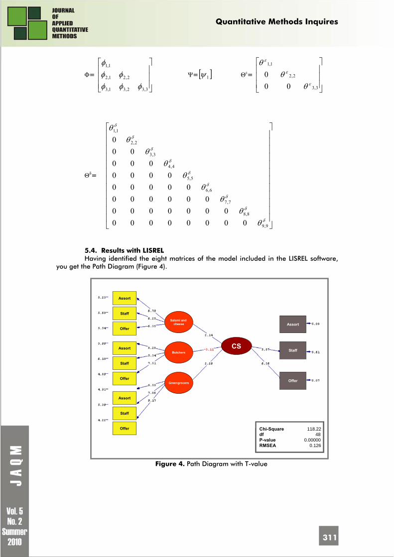
Quantitative Methods Inquires
311
Φ=
⎥⎥⎥
⎦
⎤
⎢⎢⎢
⎣
⎡
3,32,31,3
2,21,2
1,1
φφφφφ
φ Ψ= [ ]1ψ Θε=
⎥⎥⎥
⎦
⎤
⎢⎢⎢
⎣
⎡
3,3
2,2
1,1
000
ε
ε
ε
θθ
θ
Θδ=
⎥⎥⎥⎥⎥⎥⎥⎥⎥⎥⎥⎥
⎦
⎤
⎢⎢⎢⎢⎢⎢⎢⎢⎢⎢⎢⎢
⎣
⎡
δ
δ
δ
δ
δ
δ
δ
δ
δ
θθ
θθ
θθ
θθ
θ
9,9
8,8
7,7
6,6
5,5
4,4
3,3
2,2
1,1
000000000000000
00000000000
0000000
000
5.4. Results with LISREL Having identified the eight matrices of the model included in the LISREL software,
you get the Path Diagram (Figure 4).
Salami and cheese
Butchers
Greengrocers
CS
Assort
Staff
Offer
Assort
Staff
Offer
Assort
Staff
Offer
Assort
Staff
Offer Chi-Square 118.22df 48P-value 0.00000RMSEA 0.126
Salami and cheese
Butchers
Greengrocers
CS
Assort
Staff
Offer
Assort
Staff
Offer
Assort
Staff
Offer
Assort
Staff
Offer Chi-Square 118.22df 48P-value 0.00000RMSEA 0.126
Figure 4. Path Diagram with T-value
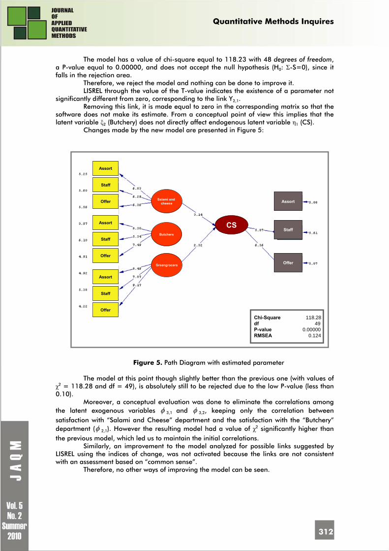
Quantitative Methods Inquires
312
The model has a value of chi-square equal to 118.23 with 48 degrees of freedom, a P-value equal to 0.00000, and does not accept the null hypothesis (H0: Σ-S=0), since it falls in the rejection area.
Therefore, we reject the model and nothing can be done to improve it. LISREL through the value of the T-value indicates the existence of a parameter not
significantly different from zero, corresponding to the link Y2,1. Removing this link, it is made equal to zero in the corresponding matrix so that the
software does not make its estimate. From a conceptual point of view this implies that the latent variable ξ2 (Butchery) does not directly affect endogenous latent variable η1 (CS).
Changes made by the new model are presented in Figure 5:
Salami and cheese
Butchers
Greengrocers
CS
Assort
Staff
Offer
Assort
Staff
Offer
Assort
Staff
Offer
Assort
Staff
Offer
Chi-Square 118.28df 49P-value 0.00000RMSEA 0.124
Figure 5. Path Diagram with estimated parameter
The model at this point though slightly better than the previous one (with values of
χ2 = 118.28 and df = 49), is absolutely still to be rejected due to the low P-value (less than 0.10).
Moreover, a conceptual evaluation was done to eliminate the correlations among the latent exogenous variables φ 3,1 and φ 3,2, keeping only the correlation between satisfaction with “Salami and Cheese” department and the satisfaction with the “Butchery” department (φ 2,1). However the resulting model had a value of χ2 significantly higher than the previous model, which led us to maintain the initial correlations.
Similarly, an improvement to the model analyzed for possible links suggested by LISREL using the indices of change, was not activated because the links are not consistent with an assessment based on “common sense”.
Therefore, no other ways of improving the model can be seen.

Quantitative Methods Inquires
313
5.5. Results with PLS The model analyzed in this case involves measuring the overall satisfaction with a
supermarket (latent variable, CS) using the satisfaction with three other latent variables, “Salami and cheeese”, “Butchers”, “Greengrocers” (Figure 6).
Salami and
cheese
Butchers
Greengrocers
CS
0.323(2.947)
0.130(1.541)
0.372(3.392)
RSq=0.492
Figura 6. Initial PLS Model
The bootstrap [11] test shows a significant link is not relevant to the relationship
between satisfaction with Butchery and customer satisfaction, giving a value of 1.541 (<2). We proceeded to the elimination of this bond and consequently the elimination of the latent variable “Butchery” (Figure 7, Table 4).
Salami and
cheese
Greengrocers
CS
0.375(4.432)
0.413(4.542)
RSq=0.482
Figure 7. Final PLS Model

Quantitative Methods Inquires
314
Table 4. Results with Bootstrap
Measurement Mode (weight)
Entire Sample Estimate
Mean of Subsamples
Standard Error T-Statistic
Assortment 0.4561 0.4585 0.0890 5.1227
Staff 0.4009 0.3969 0.0824 4.8625 Salami and cheese Goods
Offered 0.4044 0.3981 0.0789 5.1269
Assortment 0.3571 0.3524 0.0454 7.8719
Staff 0.4114 0.4181 0.0469 8.7654 Greengrocery Goods Offered
0.3910 0.3896 0 .0500 7.8133
Assortment 0.4253 0.4272 0.0493 8.6348
Staff 0.3743 0.3730 0.0419 8.9420 Customer Satisfaction Goods
Offered 0.4130 0.4157 0.0505 8.1794
Table 5. Structure Model
Structure Model
Entire Sample Estimate
Mean of Subsamples
Standard Error T-Statistic
Salami and cheese ->CS 0.3750 0.3724 0.0846 4.4319
Greengrocery ->CS 0.4130 0.4241 0.0909 4.5422
5.6. Comparison of results according to the LISREL and PLS approaches The model presented a report giving “reflective”, which can be expressed by the
covariances between the latent variables and manifest variables. This differs from the reports giving “instructive” in which the variables are used as
manifest indicators of latent variables. Regarding the validation of the model that characterizes the PLS [2] approach is the
existence of individual indices of goodness of fit (R2) is not inferential. Therefore, the results are valid only for the sample. Equally, with the LISREL model there is a global parametric index. Therefore, it is an inferential index and extended to the entire population.
The case study observed a value of R2 between 0 and 1, which makes the model acceptable.
Bootstrap analysis of the text referring to this model reveal the values of T-Statistic are all greater than 2, which means that the links are all significant, because their values fall in the rejection of the null hypothesis (H0: μ = 0).
Finally, conceptually, analysis of the model shows that the overall satisfaction with a supermarket is not directly dependent on the variable of satisfaction with the “Butchery” department. This confirms the final evaluations obtained with LISREL.

Quantitative Methods Inquires
315
6. Final remarks The verification of the conceptual model in LISREL showed that Customer
Satisfaction with a supermarket is not adequately measured by the variables considered. This means that the satisfaction with one department is not considered a serious effect on overall satisfaction. In particular, the satisfaction with the “butchery” departmetn has no significant impact on “overall satisfaction”. For this reason, the corresponding relationship is eliminated.
What led to the falsification of the model is the magnitude of the residual as a whole. It showed that a wide discrepancy between the observed matrix (S) and the matrix Hold (Σ) is not attributable to simple stochastic fluctuations. For this purpose the following were analyzed:
• the Steamleaf Plot for the distribution of residuals, which has a bell shaped curve, considering the “probability sample”
• the Q-plot for the dispersion of the standardized residuals, which shows the straight line interpolating the residuals (near 45° line), making it seem that there is a good model-to-data fit.
The sensitivity of the Chi-square to the sample size (though not particularly large), granted to the analysis of alternative measures of overall adaptation of the model:
• the GFI (goodness of fit index), where the value of the t-statistic is standardized with the maximum value it can reach (it should be between 0 and 1). The reference model is equal to 0.82 (good fit). However, this measure takes no account of degrees of freedom, so that the model is parsimonious
• the AGFI (adjusted goodness of fit index), which is a modified version of the previous year. The value obtained was 0.72 (also between 0 and 1)
• the RMR (root mean squared residuals), which represents a pure average of the squared residuals, which shows a value of 0.073. However, these measures have the disadvantage of not having a statistical distribution. For this reason, we cannot perform significance tests of the model, being valid only for the sample considered.
Having verified the proper fit of the model to data, show that the falsification of the model may be due to an incorrect formulation of the questionnaire, or the fact that other possible variables were not considered. References
1. Al-Nasser A.D. Customer satisfaction measurement models: generalized maximum
entropy approach, Pak J. Stat. 19, 2003, pp. 213–226 2. Amato, S., Espozito Vinzi, V. and Tenenhaus, M. A global goodness-of-fit index for
PLS structural equation modeling, Oral Communication to PLS Club, HEC School of Management, France, 2004
3. Amenta, P. and Ciavolino E. Restricted Co-Inertia Analysis: Uno strumento statistico per la valutazione della Customer Satisfaction, in Statistica e Applicazioni, 2005, Volume III, special number 1, Valutazione e Customer Satisfaction per la qualità dei servizi, Roma, 8-9 Settembre 2005, ISSN 1824 – 6672
4. Bollen, K. A. Structural equation with latent variables, New York, Wiley, 1989 5. Chin, W. Partial least squares for researchers: An overview and presentation of
recent advances using the PLS approach, 2000, p. 68. Available at http://disc-nt.cba.uh.edu/chin/indx.html
6. Ciavolino, E. and Al-Nasser, A. D. Comparing Generalized Maximum Entropy and Partial Least Squares methods for Structural Equation Models, Journal of nonparametric statistics, Vol. 21, Issue 8, 2009, pp.1017-1036
7. Ciavolino, E., Al-Nasser, A. D. and D’Ambra A. The Generalized Maximum Entropy Estimation method for the Structural Equation Models, 30th Annual Conference of the German Classification Society (GfKl), Berlin, Germany, 2006

Quantitative Methods Inquires
316
8. Ciavolino, E., Dahlgaard J. J. Simultaneous Equation Model based on Generalized Maximum Entropy for studying the effect of the Management’s Factors on the Enterprise Performances, Journal of applied statistics, Vol. 36, Issue 7, ISSN: 1360-0532, 2009, pp. 801-815
9. Ciavolino, E., D'Ambra, L. and De Franco, D. Massima Entropia Generalizzata e Simple Component Analysis per l’analisi della Customer Satisfaction nel Trasporto Pubblico Locale: L’Esperienza dell’Azienda, AMTS di Benevento, Rivista di economia e statistica del territorio, vol. 3, ISSN: 1971-0380, 2007, pp. 201-221
10. Ciavolino, E. and Dahlgaard J. J. ECSI - Customer Satisfaction Modelling and Analysis: A Case Study, Total Quality Management & Business Excellence, vol. 18, pp. 545-555, ISSN: 1478-3363, 2007
11. Ciavolino, E. and Meccariello, G. Un modello di regressione PLS per lo studio delle emissioni di sostanze inquinanti, Statistica & Societa, anno III, n. 3, rCe edizioni, 2005
12. Dahlgaard, J. J. and Ciavolino, E. Analysing Management Factors on Enterprise Performance, Asian journal on quality, vol. 8 n.3, ISSN: 1598-2688, 2007, pp. 1-10
13. Fornell, C., Bookstein, F. L. Two structural equation models: LISREL and PLS applied to Consumer Exit-Voice Theory, J. Market. Res. 19, 1982, pp. 440–452
14. Joreskog, K. G. A general method of estimating a linear structural equation System, in Structural Equation Models in the Social Sciences, S. A. Goldberg and D. O. Duncan, eds., Seminar Press, NewYork, 1973, pp. 85–112
15. Wold, H. Partial least squares, in Encyclopaedia of Statistical Sciences,Vol. 6, S. Kotz and N.L. Johnson, eds., John Wiley & Sons, NewYork, 1985, pp. 581–591

Quantitative Methods Inquires
317
INFORMATION THEORETIC ESTIMATION IMPROVEMENT TO THE NONLINEAR GOMPERTZ’S MODEL BASED
ON RANKED SET SAMPLING
Enrico CIAVOLINO Università Salento, Salento, Italy E-mail: [email protected]
Amajd D. AL-NASSER Yarmouk University, Irbid, Jordan E-mail: [email protected]
Abstract: The aim of this paper is to apply both Generalized Maximum Entropy (GME) estimation method and Ranked Set Sampling (RSS) technique to improve the estimations of the Gompertz’s Model. The Gompertz’s model is a simple formula which expresses the geometrical relationship between the force of mortality and age. The choice of evaluating the RSS is due to the fact that in many practical applications of the Gompertz’s model, as in biological or environmental sciences, the variable of interest is more costly to measure but is associated with several other easily obtainable. In this paper, we have used Monte Carlo experiments to illustrate the performance of the GME estimator based on two different sampling techniques: the Simple Random Sample (SRS) and RSS. Moreover, the results are compared with the traditional Maximum Likelihood Estimates (MLE). Key words: Generalized Maximum Entropy; Ranked Set Sampling; Gompertz’s Model; Maximum Likelihood Estimates; Monte Carlo experiments
1. Introduction
Gompertz’s law (Gompertz, 1865) has a very important role in modelling the human mortality rate and providing the actuarial tables. Moreover, in recent years, it has been applied to several other fields, such as in the fertility rate model (Booth, 1984), in biological medical data (Ricklefs et al., 2002), in environmental data, or in the study of reliability (Yamada et al., 1985).
In this paper, we propose the GME estimator as an alternative to Maximum Likelihood Estimation (MLE), since it is widely used in literature in cases of non linear function (Golan et al., 2001). In particular we can highlight some points:
• The GME approach uses all the data points and does not require restrictive moment or distributional error assumptions.
• Thus, unlike the MLE estimator, the GME is robust for a general class of error distributions.
• The GME estimator can be used when the sample is small, when there are many covariates, and when the covariates are highly correlated.
It means that the GME was proposed because it is particularly useful when there are no restrictive sampling assumptions or in the case of ill-posed problems or

Quantitative Methods Inquires
318
underdetermined ones, and also because in these cases MLE is unattractive and not robust to the underlying (unknown) distribution (Golan, 2008).
Moreover, RSS (McIntyre, 1952) could be used to increase the precision of estimates and to reduce costs, by using the researchers’ experiences or inexpensive measurements.
The format of this paper is as follows. In Section 2 the Gompertz’s model is introduced in its characteristics and analytical formulation by considering the MLE method. In Section 3, firstly the classic GME formulation is specified and then the Gompertz’s model is expressed in the framework of the GME. In Section 4, the RSS method is presented and a discussion on how it can be utilized for applications in which the Gompertz’s model is used. In Section 5, Monte Carlo experiments show the numerical performance for the proposed estimators, based on the RSS and SRS sampling schemes. Section 6 contains concluding remarks and discussion of future works.
2. The Gompertz’s Model
Benjamin Gompertz, in 1825, showed that the mortality rate increases in a
geometrical progression, defining one of the most informative actuarial functions for investigating the ageing process. He observed a law of geometrical progression in death rates by analysing a sample of people, aged between 20 and 60 years, in England, Sweden, and France. Gompertz’s law has become the most successful law to model the dying out process of living organisms (Willemse et al., 2000). The relationships of the force of mortality, such as the power function of age, is also called the Weibull model (Carey, 2001) and it can be expressed by the following formula:
xy B C ε= ⋅ + (1)
Where B>0 reflects the general level of mortality in the population, and C>1 is
Gompertz’s constant that reflects the rate at which the force of mortality increases with age; x>0 is the age, and y is the force of mortality at age x.
The estimates of the parameters B and C can be obtained numerically using different methods, however, the MLE is the most commonly used for this model and it is discussed by Garg et al. (1970).
The MLE estimation method, presents the assumption that the random variables Dx (number of deaths at age x before reaching age x+1) follows a Binomial distribution: B(nx, qx). The px, reported in the following formula (2), is the conditional probability function of the Gompertz’s model given in (1):
( )1 1
1 / logx x t xtx x
dt BC dt BC C Cxp e e e
μ+ +
− − − −∫ ∫= = = (2)
Or considering the log function:
log ( 1) / logxxp B C C C= − ⋅ ⋅ − and 1log / logx xp p C+ =
(3)
The other parameters are defined as follows: qx=1-px, nx is the number of people of
age x and dx is the value of the random variable Dx. Given this assumption, the logarithm of the joint likelihood function is the following:
( ) ( )log ( , ) log log 1x x x x xx
L B C n d p d p= − ⋅ + ⋅ −∑ (4)

Quantitative Methods Inquires
319
The general way of estimating the parameters is to use Nonlinear Maximization (NM), so as to find the minimum of the following function and to plug into (2) for the px:
( ) ( )( 1) / log
,min ( 1) / log log 1
xx B C C Cx x xB C x
n d B C C C d e− ⋅ ⋅ −⎡ ⎤− ⋅ ⋅ ⋅ − − ⋅ −⎣ ⎦∑ (5)
The NM problem can be solved via numerical methods such as the Newton-
Raphson iteration or the Simplex algorithm.
3. Generalized Maximum Entropy In the framework of the Information Theoretic we propose the use of the
Generalized Maximum Entropy (GME) to estimate the non linear relationship between age and the force of mortality. In this section, we start by briefly describing the traditional maximum entropy (ME) estimation method, then we introduce the GME formulation as a method for recovering information from the Gompertz’s model.
3.1. The GME estimation method The Entropy of Information was first introduced by Claude Shannon in 1948 as a
propriety associated to any probability distribution, defining an axiomatic method of measuring the uncertainty (state of knowledge) of a collection of events.
Letting X be a random variable with possible outcomes {x1, x2,…, xs}, with the corresponding probability P = {p1, p2,…, ps} such that Σpi=1, Shannon defined the entropy of information of probabilities distribution function as:
1( ) log( )s
i iiH P k p p
== − ⋅ ⋅∑ (6)
Where k is a constant usually equal to 1; and 0 ln(0)=0⋅ . The quantity {- log(pi)} is
called self information of the xi event. The average on the self information is defined as the Entropy. The function H(P) is called Entropy, Shannon’s Entropy or Information Entropy.
Edwin Thompson Jaynes (1957a, 1957b) extended the entropy of information by defining the Maximum Entropy Principle (MEP). The MEP estimates an unknown probability distribution from given moment constraints and adding up normalization constraints on the probabilities.
The frequency that maximizes entropy is an intuitively reasonable estimate of the true distribution when we lack any other information. If we have information about an experiment, such as the sample moments, or non-sample information about the random variable, such as restrictions from economic theory, we can to alter our "intuitively reasonable" estimate. The method of maximum entropy proceeds by choosing the distribution that maximizes entropy, subject to the sample and non-sample information.
Letting X be a random variable with possible outcomes {x1, x2,…, xs}, the objective of the MEP is to recover the unknown probability distribution P = {p1, p2,…, ps}, taking into account: consistency constraints, by defining the functions {f1(xi), f2(xi), …, fT(xi)}, which represents the constraints (or information) generated by the data; measurable values {y1, y2, …, yT}, obtained by a priori knowledge on the phenomenon, or by training dataset.
The constraints generated from the data and the measurable values, are expressed by the following equation:
1( )st i i tif x p y
=⋅ =∑ t = 1,2,…,T (7)
The adding up normalization constraints, which means Σpi=1, are the following:

Quantitative Methods Inquires
320
11s
iip
==∑ (8)
The MEP estimates the probability distribution by the maximization of the entropy
function, equation (6), based on the consistency and normalization constraints, equation (7, 8), where the consistency constraints are expressed in form of expectation values of a discrete random variable1:
Amos Golan et al. proposed in 1996 an alternative method to solve many standard and ill-posed econometric problems in the framework of the MEP developed by Jaynes,
This information theoretic method, which is called Generalized Maximum Entropy (GME), is based on the re-parameterization and re-formulation of a general linear model. Considering a regression model y=Xβ+ε with n units and m variables, the coefficients and the error terms can be re-parameterized as a convex combination of expected value of a discrete random variable, as in the
following equation:
,1 , ,1 ,1 , , ,1 , ,1n n m m n n m m m M m M n n N n N⋅ ⋅ ⋅ ⋅= ⋅ + = ⋅ ⋅ + ⋅y X β ε X Z p V w (9)
The matrix inner products (Z·p) and (V·w), represent respectively the re-
parameterization of the regression coefficients and the error terms as in form of expected value of a discrete random variable.
The matrices Z and V are diagonal and the generic matrix element is represented
respectively by the vectors ' [ / 2 0 / 2 ]k c c c c= − −z with {k = 1, . . . , m} and ' [ / 2 0 / 2 ]h b b b b= − −v with {h = 1, . . . , n}.
These vectors (zk and vh) define the support values, called fixed points, usually with five elements (M=N=5) with a given constants ‘c’ and ‘b’, uniformly and symmetrically chosen around zero with equally spaced distance discrete points, or as Golan suggested, for the error terms, to follow the six-sigma rule (Pukelshiem, 1994), where the number of fixed points is 3, and the constant c is equal to ys
).
The super vectors p and w associated are probabilities and have to be estimated by maximization of the Shannon entropy function:
' '1, ,1 1, ,1( , ) ln lnm M m M n N n NH p w ⋅ ⋅ ⋅ ⋅= − ⋅ − ⋅p p w w
subjected to some normalization and consistency constraints. The steps for the GME
algorithm are shown in the following table 1. Table 1. The Generalized Maximum Entropy Algorithm 1. Re-parameterize the unknown parameters and the disturbance terms as a convex combination of expected value of a discrete random variable; 2. Re-formulate the model with the new re-parameterization as the data constraint; 3. Define the GME problem as non-linear programming problem in the following form:
Objective Function = Shannon’s Entropy Function 1. The consistency constraints, which represents the new formulation of the model; 2. The normalization Constraints. 4. Solve the non-linear programming by using numerical method
The constraints defined for estimating the unknown parameters refer to consistency
and normalization constraints. The first one represents the information generated from the

Quantitative Methods Inquires
321
data, that means a part of the model defined in the equation (9); the second one identifies the conditions: 0≤pkj≤1, {j=1, …,M; k=1,…,m}, ∑pkj=1 {k=1,…,m} and 0≤whj≤1, {j=1,…,N; h=1,…,n}, ∑whj=1 {h=1,…,n}.
The main advantages of using GME estimation method, as above defined (supra § 1), are its desirable properties which can be briefly summarized: does not require restrictive moments or distributional error assumptions; it’s robust for a general class of error distributions; may be used with small samples, with many highly correlated covariates; moreover, using the GME method, it is easy to impose nonlinear and inequality constraints.
Therefore the GME works well in case of ill-behaved data and the above listed cases, where the MLE estimator cannot proceed.
In the following section the GME formulation for the Gompertz’s model is explained, moreover the definition of the optimization function and both consistency and normalization constraints will be discussed.
3.2. GME for the Gompertz’s Model The GME formulation as a method for recovering information from the Gompertz’s
model, starts from the relationship between the age and the force of mortality, expressed by:
,1,1 ,1
nn nB C= ⋅ +xy ε (9)
The starting point, following the algorithm in table 1, is the re-parameterization of
the unknown parameters and error terms, as a convex combination of excepted values. For the Gompertz’s model, the number of predictor variables is just one, age, which means, as in the above general formulation, m=1 and the matrix Z is just a vector
' [ / 2 0 / 2 ]k c c c c= − −z , considering M=5 fixed points. The error term is obtained
by considering the diagonal matrix with generic element ' [ 3 0 3 ]k y ys s= − ⋅ ⋅v ) ), based on
the three-sigma rule, with N=3 fixed points. The re-parameterization as convex combination of expected values is expressed in
the following equations:
'1, ,1M MB = ⋅z p (10) '1, ,1M MC = ⋅c q (11)
,1 , ,1n n n N n N⋅ ⋅= ⋅ε V w (12)
Moreover, normalization constraints are necessary, because for each probability
vector of the coefficients and error terms (ex., pM,1), the sum of probabilities estimated have to be equal to 1, which means ∑pj=1 , ∑qj=1 and ∑whj=1 {h=1, …, n}.
These constraints are formalized by the following expressions:
'1, ,1 1M M⋅ =p 1 (13) '1, ,1 1M M⋅ =q 1 (14) *
, ,1 ,1n n N n N n⋅ ⋅⋅ =J w 1 (15)
The matrix J* is the Kronecker product between the identity matrices In,n and the
vector of one 1M,1, which means *, , 1,( )n n N n n N⋅ ′= ⊗J I 1 :

Quantitative Methods Inquires
322
*, ,1 ,1n n N n N n⋅ ⋅⋅ =J w 1 =>
1
2
111 1111 1
111 1n n n
⎡ ⎤ ⎡ ⎤ ⎡ ⎤⎢ ⎥ ⎢ ⎥ ⎢ ⎥⎢ ⎥ ⎢ ⎥ ⎢ ⎥⋅ =⎢ ⎥ ⎢ ⎥ ⎢ ⎥⎢ ⎥ ⎢ ⎥ ⎢ ⎥⎢ ⎥ ⎢ ⎥ ⎢ ⎥⎣ ⎦ ⎣ ⎦ ⎣ ⎦
0 0 w0 0 w
0 0 w
L
L
M M O M M M
L
(16)
Given the re-parameterization, the Gompertz’s model can be re-formulated in the
following way, where all the parameters, unknowns and error terms, are expressed as expected values:
( ) ( ) ,1' ',1 1, ,1 1, ,1 , ,1
n
n M M M M n n N n N⋅ ⋅= ⋅ ⋅ ⋅ + ⋅x
y z p c q V w (17)
The definition of GME problem as non linear programming problem is the following:
Objective function: Max ' ' '( , , ) ln ln lnH P Q W = − ⋅ − ⋅ − ⋅p p q q w w
Consistency Constraints: ( ) ( ) ,1' ',1 1, ,1 1, ,1 , ,1
n
n M M M M n n S n S⋅ ⋅= ⋅ ⋅ ⋅ + ⋅x
y z p c q V w
Normalization Constraints: '1, ,1 1M M⋅ =p 1 ; '
1, ,1 1M M⋅ =q 1 ; *, ,1 ,1n n N n N n⋅ ⋅⋅ =J w 1
The non-linear programming system is solved by the formulation of the Lagrangian
function and the first order conditions which provides the basis for the solution. The Lagrangian function is expressed by the following formulation:
( ) ( )' ' ' ' ' '
' ' ' *
ln ln ln
1 1
L
θ ν
⎡ ⎤= − ⋅ − ⋅ − ⋅ + ⋅ − ⋅ ⋅ ⋅ − ⋅ +⎢ ⎥⎣ ⎦⎡ ⎤ ⎡ ⎤ ⎡ ⎤+ ⋅ − ⋅ + ⋅ − ⋅ + ⋅ − ⋅⎣ ⎦ ⎣ ⎦ ⎣ ⎦
xp p q q w w λ y z p c q V w
p 1 q 1 τ 1 J w
(18) where θ, ν, λ, τ, are respectively the scalars and the vectors of the Lagrangian
multipliers. By taking the gradient of L it is possible to derive the first-order-condition. However, the equations system will not be in closed form and to get the final values, a numerical optimization technique (successive quadratic programming method) should be used to compute probabilities (Ciavolino, 2007).
The estimations can be expressed by:
'1, ,1
ˆ ˆM MB = ⋅z p (19)
'1, ,1
ˆ ˆM MC = ⋅c q (20)
, ,1ˆ ˆn n S n Sε ⋅ ⋅= ⋅V w (21)
Respectively for the general level of mortality (19), the force of mortality (20) and
the error term (21).
4. Ranked Set Sampling Method The concept of Ranked Set Sampling is a recent development that enables more
structure to be provided to the collected sample items, although the name is a bit of a misnomer as it is not as much a sampling technique as a data measurement technique.

Quantitative Methods Inquires
323
This approach to data collection was first proposed by McIntyre in 1952, for situations where taking the actual measurements for sample observations is difficult (e.g., costly, destructive, time-consuming), but mechanisms for either informally or formally ranking a set of sample units is relatively easy and reliable.
In particular, McIntyre was interested in improving the precision in estimation of average yield from large plots of arable crops without a substantial increase in the number of fields from which detailed, expensive and tedious measurements needed to be collected. For discussions of some of the settings where ranked set sampling techniques have found application, see Chen et al. (2004).
The idea of using the RSS for the Gompertz’s model, is in some practical applications, where the response variable is too expensive to measure , destructive or time-consuming, but but the predictor variable can be measured easily with relatively negligible cost.
Some examples can be found in studies in the ecological or biology fields, where, for instance, the death rate of plants or insects caused by the contamination in hazardous waste sites are analyzed using the Gompertz’s law. The analysis can be improved by inspections for ranking areas of soil based on visual inspection or other expert opinion about the sample units (Chen et al., 2004).
The scheme we used in this study is the balanced RSS, which involves drawing m sets of Simple Random Samples, each of size m from a population, and ranking each set with respect to the variable of interest, for instance the age. Then, from the first set, the element with the smallest rank is chosen for the actual measurement. From the second set, the element with the second smallest rank is chosen. The process is continued until we have selected the largest unit from the last simple random sample.
The procedure can be formalized as the following steps: 1. Select m2 units randomly from the population. 2. Randomly allocate the m2 units into m subsets, each of size m. 3. Order the units within each subset, based on the perception of the interest
variable. 4. In the RSS, the smallest unit in the first subset is selected for actual
measurement, the second smallest unit in the second subset is selected for actual measurement, we continue in this process until the largest ranked unit is selected from the mth subset.
5. These four steps are called cycle and can be repeated r times until the desired sample size is reached, equal to n r m= ⋅ .
If just three ranks and one cycle are considered, the selected RSS is denoted by: {X[1], X[2], X[3]}. In order to select a RSS with a sample size equal to n r m= ⋅ , the cycle is repeated r independent times, yielding the following sample:
{ }[1], [2], [ ],, ,..., , 1,...,j j m jX X X for j r= (22)
It can be noted that the selected elements are mutually independent order statistics but not identically distributed. In practice, the set size m is kept small to ease the visual ranking, RSS literature suggested that m = 2, 3, 4, 5 or 6.
Table 2. Ranked Set Sampling Design
Rank (m=3) Cycle (r=4) Young Adult Elderly
X[1],1 - - 1 - X[2],1 - - - X[3],1 X[1],2 - -
2 - X[2],2 - - - X[3],2 X[1],3 - -
3 - X[2],3 -

Quantitative Methods Inquires
324
- - X[3],3 X[1],4 - -
4 - X[2],4 - - - X[3],4
Table 2 shows an illustrative example, where the set size m is equal to 3 (the
number of ranks) and the cycles r = 4. In the table, we assume that the units are selected according to their age, therefore there are three ranks: Young, Adult, Elderly, and the rows represent the ordered sample within each cycle, where X[i],j is the sample unit included in the RSS, which represents the ith order unit in the jth cycle.
The number of units randomly selected are 36, m2=32=9, for 4 cycles, but only 12 are included in the RSS.
5. Simulation and Results We perform different simulation studies in order to draw conclusions about the
performance of GME and MLE estimation methods for the Gompertz’s model by using the RSS technique. The simulation experiments start with the analysis of the fixed points to evaluate the sensitivity of the GME for the Gompertz’s model. The analysis of the sensitivity is made by changing the value of the constant ‘c’ and the number of the fixed points. This analysis is recommended and useful (Golan et al., 1996), to verify the support spaces on the coefficients and error terms to measure the sensitivity of results across support space specifications.
Four simulation experiments are considered to measure the sensitivity of the GME estimator: the first two simulations, to determine the variance and the bias of the Gompertz’s coefficients; the last two simulations, to examine the variance and the bias of the error terms.
The sensitivity analysis is measured in term of Bias and Mean Squared Error (MSE), as in the following equations for the B coefficient:
( )11
ˆ( ) nii
Bias B n B B−=
= ⋅ −∑
( )211
ˆ( ) ni ii
MSE B n B B−=
= ⋅ −∑
After the sensitivity simulation studies, that allow to choose the best support space
specification for the GME estimator, we performed two simulation studies for the evaluation GME and MLE performance based on the SRS and RSS.
The measures Bias and MSE are used to evaluate the performance of the estimator applied to both sampling techniques, computing also relative efficiency (eff); where the eff of B is defined as:
( )( )( )
GME
MLE
MSE Beff BMSE B
=
To perform all the simulation studies, the parameters of the Gompertz’s function B
and C were first initialized to 0,3 and 2. Using these values as initial values, a simulation study was carried out by generating 1000 samples according to the following relationship:
0,3 (2) ixi iy ε= ⋅ + , i = 1,2,...,n (23)

Quantitative Methods Inquires
325
where ε ~ N(0,1) and X ~ Exp(1). The sensitivity simulation studies for the GME parameters choice were conducted by fixing the sample size to be 20.
All the pseudo distributions varieties are generated from a build in subroutines of International Mathematical and Statistical Library (IMSL). The solution of GME system were solved and generated by using a successive quadratic programming method to solve a nonlinear programming problems based on the NCONF and NLPQL subroutines. The basic FORTRAN codes for computational purposes were developed by Schittkowski (1986) and necessary modifications were made by the authors.
5.1. The Sensitivity Analysis of the GME Estimates Tables 3, 4, 5 and 6 show the results of the sensitivity analysis for the fixed points. It
has been considered four experiments: the first two to evaluate the support value ‘c’ and the number of fixed points for the parameters B and C; the last two for the error term (supra § 3).
Experiment 1. This experiment is performed to select the support parameter
bounds of B and C. we start by using only three support values for each of these parameters in the interval [-c, 0, c], where c = 1, 5, 10, 50 or 100. The support bounds of the error term are fixed to be three data points selected according to the three sigma rule. The results of this simulation study are given in Table.3. The results indicated that the GME estimates were more accurate and more efficient than the MLE estimates for all the selected support bound. However, the best support bound should be selected in the interval [-5, 0, 5] for both parameters, which; almost, gives the minimum MSE and bias for the GME estimates.
Table 3. Selecting the ‘c’ value of the parameters (B e C) support points
METHODS GME: different ‘c’ VALUES of the fixed points
PARAMETERS [-1, 1] [-5, 5] [-10, 10] [-50, 50] [-100, 100]
MLE
B Bias -0,0098 -0,0107 -0,0097 -0,0114 -0,012 0,1715
MSE 0,0108 0,011 0,0115 0,0153 0,0131 0,0394
C Bias -0,0159 -0,0029 -0,0092 0,0171 0,0141 0,0504
MSE 0,0028 0,0022 0,0023 0,0026 0,0028 0,0034
Experiment 2. This experiment is repeated under the same assumptions of
experiment two, and by fixing the support bounds of the parameters in the interval [-5, 5]. The aim now is to determine the number of support points within the suggested interval that leads to better results. Consequently, we start to increase the numbers of support points and allocate them in an equidistant fashion. The results of this experiment in Table. 4 suggested that there is no statistical improvement of the estimators if we increase the number of support points from 3 to 7 data points. Therefore, according to this simulation experiment, we suggest to fix the number of support points to be three in the interval [-5, 5].
Table 4. Fixing the number of support points for the parameters (B e C)
METHODS GME: Different NUMBERS of fixed points in [-5 5]
PARAMETERS 3 4 5 6 7
MLE
B Bias -0,0107 -0,0071 -0,0104 -0,0077 -0,0098 0,1715
MSE 0,011 0,0128 0,0118 0,014 0,0128 0,0394
C Bias -0,0029 -0,0136 -0,0112 -0,008 -0,0077 0,0504
MSE 0,0022 0,0024 0,0023 0,0024 0,0021 0,0034

Quantitative Methods Inquires
326
Experiment 3. We conducted a sampling experiment based on the experimental design outlined above and based on the results of experiment 1 and experiment 2. Hereafter, the support bounds of the error term is selected in the interval [-c Sy, 0, c Sy], then we start changing the value of ‘c’ to be equal to 1, 2, 3, 4 and 5. The results of this experiment in Table 5 indicate that the best value for ‘c’ is 3, this result is consistent with the results of Golan et al (1996), which suggest in using the three sigma rules when we setup the support bonds of the error terms.
Table 5. Selecting the ‘c’ value for the error term
METHODS GME: different ‘c’ VALUES of the fixed points
PARAMETERS [-1S, 1S] [-2S, 2S] [-3S, 3S] [-4S, 4S] [-5S, 5S]
MLE
B Bias -0,0067 -0,0107 -0,0107 -0,0117 -0,0139 0,1715
MSE 0,0107 0,0114 0,011 0,0129 0,014 0,0394
C Bias -0,0144 -0,0143 -0,0029 -0,0098 -0,0111 0,0504
MSE 0,0023 0,0021 0,0022 0,0019 0,0018 0,0034
Experiment 4. Likewise experiment 2, the simulation trial were repeated by shifting the support points of the error term to be equally spaced in the interval [-3 Sy, 0, 3 Sy]. The results of this experiment are in Table 6 suggested that we should fix three support values of the error term according to the three sigma rule.
Table 6. Fixing the number of support points for the error term
METHODS GME: different ‘c’ VALUES of the fixed points
PARAMETERS 3 4 5 6 7
MLE
B Bias -0,0107 -0,0003 -0,0032 -0,0005 -0,0023 0,1715
MSE 0,011 0,0169 0,0191 0,0168 0,0165 0,0394
C Bias -0,0029 -0,0138 -0,0092 -0,0127 -0,0161 0,0504
MSE 0,0022 0,0021 0,0028 0,0022 0,0021 0,0034
5.2. Performance Analysis of the RSS technique In this section, based on the main simulation conditions and the results of the last
four experiments, we are comparing between two the estimation methods from the view of point of the sampling techniques. Two experiments were performed, the first one based on SRS and the other one based on RSS. Noting that, in the RSS scheme the ranking done based on the X variable. Other ranking schemes could be used such as Double RSS (Al-Saleh and Al-Kadiri, 2000), which is not of our interest in this paper, to be an alternative to the classical ranking scheme.
Experiment 5. Based on the results of experiment 1 to experiment 4, by selecting
three support values for each of the parameters in the [-5, 5] interval and three support values the error term according to the three sigma rule, this experiment, under the simulation assumption outlined above, is conducted by increasing the sample size n, i.e., n = 20, 25, 30, 40 and 50. The results in Table 7 indicate that the GME is more accurate and more efficient than the MLE estimates for all sample sizes.

Quantitative Methods Inquires
327
Table 7. Comparisons between GME and MLE using SRS C B N Method
Bias MSE eff Bias MSE eff GME -0,0029 0,0022 -0,0107 0,0110 2
0 MLE 0,0504 0,0034 1,54 0,1715 0,0394
3,58
GME -0,0150 0,0029 0,0043 0,0138 25 MLE 0,0496 0,0033
1,14 0,1597 0,0337
2,44
GME -0,0085 0,0029 -0,0005 0,0096 30 MLE 0,0510 0,0035
1,21 0,1726 0,0395
4,11
GME -0,0046 0,0018 -0,0006 0,0090 40 MLE 0,0474 0,0030
1,67 0,1663 0,0368
4,09
GME -0,0013 0,0012 0,0007 0,0086 50 M
LE 0
,0429 0
,0025
2,08 0
,1482 0
,0289
3,36
Experiment 6. The aim of this experiment is to improve the simulation results by
using the simulated RSS. For the RSS sampling scheme we used a set size r = 4 or 5 and the number of cycles m = 5,6,8 and 10; to achieve the desired sample size. The results of this experiment are given in Table 8.
Table 8. Comparisons between GME and MLE using RSS
C B r m Method Bias MSE Ef
f Bias MSE ef
f GME 0,0005 0,0056 0,0039 0,0059
5 4 MLE 0,0532 0,0099
1,76 0,1938 0,0505
8,55
GME -0,0302 0,0053 0,0154 0,0144 5 5
MLE 0,0543 0,0098 1,85 0,1953 0,0511
3,55
GME -0,0101 0,0025 -0,0003 0,0128 6 5
MLE 0,0551 0,0041 1,64 0,1917 0,0499
3,89
GME -0,0179 0,0032 -0,0161 0,0107 8 5
MLE 0,0506 0,0039 1,22 0,1726 0,0405
3,78
GME 0,0078 0,0033 -0,0003 0,0084 10 5
LE 0
,0535 0
,0034
1,03 0
,1929 0
,0514
6,12
We conclude by summarizing our findings: 1. In this study we used simulated ranked data with GME and MLE estimation
methods to estimate the parameters of the Gompertz’s model. 2. Under the simulation assumptions, GME based on both sampling techniques
SRS and RSS gives a better estimate than MLE from the MSE point of view. The simulated efficiency score is more than 1 in both experiments for all parameters and under different sample sizes.
6. Conclusions and Discussion
To sum up, we consider fitting the Gompertz’s model by two different estimation
methods MLE and GME and based on two different sampling techniques: SRS and RSS. Despite the sampling technique, the simulation results demonstrate that the GME estimates are superior and often more efficient than MLE estimates in terms of MSE.

Quantitative Methods Inquires
328
Table 9. Simulation results GME (SRS vs RSS)
B C N Method
Bias MSE Eff Bias MSE eff
SRS -0,0107 0,0110 -0,0029 0,0022 20
RSS 0,0039 0,0059 1,86
0,0005 0,0056 0,39
SRS 0,0043 0,0138 -0,015 0,0029 25
RSS 0,0154 0,0144 0,96
-0,0302 0,0053 0,55
SRS -0,0005 0,0096 -0,0085 0,0029 30
RSS -0,0003 0,0128 0,75
-0,0101 0,0025 1,16
SRS -0,0006 0,0090 -0,0046 0,0018 40
RSS -0,0161 0,0107 0,84
-0,0179 0,0032 0,56
SRS 0,0007 0,0086 -0,0013 0,0012 50
RSS -0,0003 0,0084 1,02
0,0078 0,0033 0,36
For all situations used in the simulation study considering different sample size, the
GME estimates are more efficient and more accurate than the MLE estimates. However, there is no improvement in parameter estimation by MLE rely on RSS.
However, Table 9 shows the results obtained by comparing the SRS and RSS sampling schemes in the context of GME. We find out that they are comparable and no method is better than any other method, therefore, we can used GME as a robust estimation method to fit Gompertz’s model whatever the sample technique is used.
Moreover it is widely shown in the literature that in empirical circumstances, the RSS can be employed to gain more information than SRS while keeping the cost of, or the time constraint on, the sampling about the same.
Consequently, the GME estimator based on any sampling scheme can be
recommended for estimating the parameter of Gompertz’s model as an alternative
estimation method to the classical MLE.
Moreover, other statistical procedures and new methodologies in the context of RSS
are proposed, like extreme ranked set sampling (ERSS), median ranked set sampling (MRSS)
or L ranked set sampling (LRSS) by Al-Nasser (2007). It may be useful to investigate these
different methods for the Gompertz’s model, considering the GME estimator.
References
1. Al-Nasser A. D. L Ranked Set Sampling: A Generalization Procedure for Robust Visual Sampling, Communications in Statistics—Simulation and Computation, 36, 2007, pp. 33–43
2. Al-Saleh, M. F. and Al-Kadiri, M. Double ranked set sampling, Statistical Probability Letter, 48, 2000, pp. 205-212
3. Booth H. Transforming Gompertz's Function for Fertility Analysis: The Development of a Standard for the Relational Gompertz Function, Population Studies, Vol. 38, No. 3, Nov. 1984, pp. 495-506
4. Carey, J.R. Insect biogeography, Ann. Rev. Entomol. 46, 2001, pp. 79–110 5. Chen, Z., Bai, Z.D. and Sinha, B. K. Ranked Set Sampling: Theory and Applications,
New York: Springer- Verlag, 2004

Quantitative Methods Inquires
329
6. Ciavolino, E. Modelling GME and PLS estimation methods for evaluating the Job Satisfaction in the Public Sector, QMod’07, University of Helsingborg, Sweden, 18 – 21 June 2007, June 2007, Linköping University Electronic Press, ISSN number: 1650-3740
7. Ciavolino, E. and Dahlgaard, J. J. Simultaneous Equation Model based on Generalized Maximum Entropy for studying the effect of the Management’s Factors on the Enterprise Performances, Journal of Applied Statistics, Vol. 36, Issue 7, 2009, pp. 801 – 815
8. Ciavolino, E. and Al-Nasser, A. D. Comparing Generalized Maximum Entropy and Partial Least Squares methods for Structural Equation Models, Journal of Nonparametric Statistics, Vol. 21, Issue 8, 2009, pp.1017 - 1036
10. Garg M. L., Rao B. R. and Redmond C. K. Maximum-Likelihood Estimation of the Parameters of the Gompertz Survival Function, Applied Statistics, Vol. 19, No. 2. 1970, pp. 152-159
11. Golan, A. Information and Entropy Econometrics — A Review and Synthesis, Foundations and Trends in Econometrics, 2, 1–2, 2008, pp. 1–145
12. Golan, A., Judge, G. and Karp, L. A maximum entropy approach to estimation and inference in dynamic models or counting fish in the sea using maximum entropy, Journal of Economic Dynamics and Control, 20, 2000, pp. 559-582
13. Golan, A., Karp, L. S. and Perloff, J. Estimating Coke's and Pepsi's Price and Advertising Strategies, Journal of Business & Economic Statistics, Vol. 18, No. 4, Oct. 2000, pp. 398-409
14. Golan, A., Perloff, J. M. and Shen, E. Z. Estimating a Demand System with
Nonnegativity Constraints: Mexican Meat Demand, The Review of Economics and Statistics, Vol. 83, No. 3., Aug., 2001, pp. 541-550
15. Golan, A., George, G. and Miller, D. Maximum Entropy Econometrics, Wiley, London, 1996
16. Gompertz, B. On the nature of the function expressive of the law of human mortality and on the new mode of determining the value of life contingencies, Philosophical Transactions of Royal Society A 115, 1825, pp. 513–580.
17. H. L. Rietz On Certain Properties of Makeham's Laws of Mortality with Applications, The American Mathematical Monthly, Vol. 28, No. 4, Apr., 1921, pp. 158-165.
18. Jaynes E.T. Information Theory and Statistical Mechanics, The Physical Review 106 (4), 620-630, May 15, 1957a
19. Jaynes E.T. Information Theory and Statistics Methods II, The Physical Review. 108, pp.171-90, 1957b
20. Jaynes, E. T. Prior Probabilities, IEEE Transactions On Systems Science and Cybernetics, vol. sec-4, no. 3, 1968, pp. 227-241
21. Mahajan V., Muller E. and Bass F. M. New Product Diffusion Models in Marketing: A Review and Directions for Research, Journal of Marketing, Vol. 54, No. 1, Jan. 1990, pp. 1-26
22. McIntyre, G. A. A method of unbiased selective sampling using ranked sets, Australian J. Agricultural Research, 3, 1952, pp. 385-390
23. Pukelsheim, F. The Three Sigma Rule, The American Statistician, 48(2), 1994, pp. 88–91
24. Ricklefs R. E., Scheuerlein A. Biological Implications of the Weibull and Gompertz Models of Aging, The Journals of Gerontology Series A: Biological Sciences and Medical Sciences 57:B69-B76, 2002
25. Schittkowski, K. NLPQL: A FORTRAN subroutine solving constrained nonlinear programming problems, Annals of Operations Research, 5, 1986, pp. 485–500

Quantitative Methods Inquires
330
26. Shannon C. E. A mathematical Theory of Communications, Bell System Technical Journal, 27, 1948, pp. 379–423
27. Sinha, B. K., Sinha, B. K., and Purkayastha, S. On some aspects of ranked set sampling for estimation of normal and exponential parameters, Statist. Decisions 14, 1996, pp. 223–240
28. Willemse W. J. and Koppelaar H. Knowledge Elicitation of Gompertz’ Law of Mortality, Scand. Actuarial J., 2000, 2, pp.168 -179
29. Wolfe D. A. Ranked Set Sampling: an Approach to More Efficient Data Collection, Statistical Science, Vol. 19, No. 4, 2004, pp. 636–643
30. Yamada S. and Osaki S. Software Reliability Growth Modeling: Models and Applications, IEEE Transactions on Software Engineering, vol. 11, no.12, Dec. 1985, pp. 1431-1437
1 The estimates will not be in closed form and to get the final values, a numerical optimization technique (successive quadratic programming method) should be used to compute probabilities.

Quantitative Methods Inquires
331
THE RASCH MODEL FOR EVALUATING ITALIAN STUDENT PERFORMANCE1
Ida CAMMINATIELLO University of Naples Federico II, Naples, Italy E-mail: [email protected]
Michele GALLO University of Naples L’Orientale, Naples, Italy E-mail: [email protected]
Tullio MENINI University of Naples L’Orientale, Naples, Italy E-mail: [email protected]
Abstract: In 1997 the Organisation for Economic Co-operation and Development (OECD) launched the OECD Programme for International Student Assessment (PISA) for collecting information about 15-year-old students in participating countries. Our study analyse the PISA 2006 cognitive test for evaluating the Italian student performance in mathematics, reading and science comparing the results of different local governments. For this purpose the most proper statistic methodology is Item Response Theory - IRT that collects several models, the simplest is Rasch Model – MR (1960). As the items used in the analysis are both dichotomous that polytomous, we apply Partial Credit Model (PCM). Key words: Programme for International Student Assessment; Italian student performance; Partial Credit Model 1. Introduction
The prosperity of countries now derives to a large extent from their human capital.
This consciousness urges many countries to monitor students’ learning. Comparative international assessments can extend and enrich the national picture by providing a larger context within which to interpret national performance. In response to this need, the Organisation for Economic Co-operation and Development (OECD) launched the OECD Programme for International Student Assessment (PISA) in 1997.
The PISA surveys have been designed to collect information about 15-year-old students in participating countries. PISA examines how well students are prepared to meet the challenges of the future, rather than how well they master particular curricula. PISA

Quantitative Methods Inquires
332
surveys take place every three years. The first survey took place in 2000, the second in 2003 and the third in 2006. For each assessment, one of the three areas (science, reading and mathematics) is chosen as the major domain and given greater emphasis. The remaining two areas, the minor domains, are assessed less thoroughly. In 2000 the major domain was reading; in 2003 it was mathematics and in 2006 it was science. the results of these surveys have been published in a series of reports (OECD, 2001, 2003, 2004, 2007) and a wide range of thematic and technical reports.
In this paper we focus on the PISA 2006 survey. In all countries the survey includes: • a cognitive test for evaluating the student performance • a student questionnaire to collect information from students on various
aspects of their home, family and school background • a school questionnaire to collect information from schools about various
aspects of organisation and educational provision in schools. As in previous surveys, additional questionnaire material was developed, which was
offered as international options to participating countries. In PISA 2006, two international options were available, the Information Communication Technology (ICT) familiarity and the parent questionnaire.
The PISA 2006 results show wide differences in the performance of countries that participated to the survey. Also the Italian results show performance differences within the country, in particular between local governments and between different schools (INVALSI, 2007).
Our study analyses the cognitive test for evaluating the Italian student performance in reading, mathematics and science, comparing the results of different local governments. Several papers show the measures obtained by students, we are going to focus on measurement instrument for studying:
• the abilities required by PISA 2006 test to which the Italian students are or not able to answer;
• if the students of a local government are scoring better than the students of another local government on an item (Differential Item Functioning, DIF).
For this purpose the most proper statistic methodology is Item Response Theory - IRT (Baker & Kim 2004), that collects several models, the simplest is Rasch Model – MR (1960). As the items used in the analysis are both dichotomous that polytomous, we apply Partial Credit Model (PCM).
2. Rasch model
The aim of the IRT is to test people. Hence, their primary interest is focused on
establishing the position of the individual along some not directly observable dimension called latent trait. Because of the many educational applications the latent trait is often called ability.
The IRT derives the probability of each response as a function of the latent trait and some item parameters. The same model is then used to obtain the likelihood of ability as a function of the actually observed responses and, again, the item parameters. The ability value that has the highest likelihood becomes the ability estimate. For this purpose IRT makes the important assumption of local independence. This means that the responses given to the separate items in a test are mutually independent given ability.
The objective of each IRT model is to predict the probability that a person will give a certain response to a certain item. People can have different levels of ability, and items can have different levels of ability. To keep track of this, we denote the probability of a correct response with snP , : the index s refers to the item, and the index n refers to the person. When
an item allows for more than two options, we denote the probability with xsnP ,, where the
index x refers to the options. The simplest IRT model is the RM. Rasch’s basic idea is that the Models for
Measurement make it possible to measure properly, and, equally importantly, to validate

Quantitative Methods Inquires
333
which data conform to measurement and which does not: Rasch has specified demands for a social sciences measurement to be of the same quality as measurements in the natural sciences and he has then found out exactly which kind of statistical models conform to these specified requirements, namely the Models for Measurement (Rasch, 1968). The conclusion therefore is that a given data set yield measurements in Rasch’s well-defined meaning of the word, if, and only if, the data conform to one of the Models for Measurement. So, if the Models for Measurement did not describe the data, then, in certain situations, it is considered better to discard the data than the model.
This view of Rasch’s upon data is indeed controversial and quite a contrast to the traditional approach where the statistical model is expanded to fit the data. Closely connected to the Models for Measurement is the concept of specific objectivity, which by and large is the name Rasch chose for his requirements for measurements.
For a dichotomous item the RM has only one item parameter. The probability of a correct response given l’item parameter sδ , and the person parameter nβ ,is
)exp(1)exp(
,sn
snsnP δβ
δβ−+
−= (1)
where sδ characterizes the difficulty of item s, and nβ characterizes the ability of
examinee n. The literature offers a number of alternative procedures for estimating parameters,
including Joint maximum likelihood, Conditional maximum likelihood (CML) and Marginal maximum likelihood (MML). Under appropriate assumptions these solutions are asymptotically equivalent, consistent and multivariate normal (Haberman, 1977; de Leeuw & Verhelst, 1986).
When the items are polytomous with a different number of categories which have not the same distance, the most proper version of the IRT is the Partial Credit Model (PCM) proposed by Wright & Masters (1982). The probability that a subject n answers to a item s through the category x ( sMwx ,,,,2,1 LL= ) is calculated by tht formula:
( )[ ]
( )[ ]∑ ∑
∑
= =
=
+−
+−=
sM
w
w
jjsjn
x
jjsjn
nsxP
0 0
0
exp
exp
τδβ
τδβ (2)
sjδ characterizes the difficulty of item s, for the threshold j and jτ are category
thresholds. 2.1. Rasch diagnostics In literature there are different tools to evaluate the goodness of fit of the model to
observed data. One of the most used is based on the residuals analysis for each individual (or item). The residual can be standardized as follows:
ns
nsnsns w
Exz −=
where nsw is the estimated variance of responses reproduced by model, nsx is the
response of the individual n to the item s and Ens is the expected value of the response.

Quantitative Methods Inquires
334
The interpretation of standardised residuals is simple but too analytic because it is referred to each individual or item. For obtaining a synthetic information, the mean value of
squared standardised residuals 2nsz can be calculated: ∑ =
=K
s nsn zK
U1
21 for each individual
where K is the number of items and ∑ ==
H
n nss zH
U1
21 for each item where H the number of
individuals. The expected value of nU and sU (outfit or Unweighted Mean Square statistic) is
equal to 1. However Linacre proposes different ranges around 1 according to the origin of observed data: for small samples and/or tests with few items, there is a good fit if the statistics is in the range [0.6; 1.4]; otherwise the values should be in [0.8; 1.2]. Anyway values greater than 2 are bad for the measurement .
It can be demonstrated that the outfit statistics is sensitive to big differences between β e δ ; for balancing this characteristic it is possible to weigh the squared residuals with the variance, obtaining another synthetic statistics defined INFIT (or Weighted
Mean Square statistic): ( )( )∑
∑=
== K
s ns
K
s nsnsn
w
zwV
1
12
for each individual where K is the number of
items and ( )( )∑
∑=
== H
n ns
H
n nsnss
w
zwV
1
12
for each item where H the number of individuals
The infit statistic is sensitive to unexpected behaviour affecting responses to items
near the person ability level and the outfit statistic is outlier sensitive, so it is useful to calculate both the statistics.
With reference to the estimations of parameters of RM nβ̂ and sδ̂ it is possible to
calculate the Standard Error (SE): ( )
21
1
1)ˆ(⎥⎥⎦
⎤
⎢⎢⎣
⎡=
∑ =
K
s nsn
wSE β , and
( )
21
1
1)ˆ(⎥⎥⎦
⎤
⎢⎢⎣
⎡=
∑ =
H
n nss
wSE δ
Producing a synthesis with respect to the SE of estimations sδ̂ it is possible to
calculate the mean square error: ( )[ ]∑ ==
K
s sSEK
ME1
22 ˆ1 δδ the squared root of which
supplies the mean error of item calibration δME .
The ratio between such value and the squared root of unbiased variance δSA gives
the separation index: δ
δδ ME
SASI = where ( )22δδδ MESSA −= and ∑ =
=K
s sKS
122 1 δδ is the
variance of estimations sδ̂ . If the index is far from one, the item are well separated.
In terms of the separation index, realiability index can be expressed as follow:
2
2
2
2
2
2
11 δ
δ
δ
δ
δ
δδ S
MESSA
SISIRE −==+
= . It has the property that 0=δRE if there is no
reproducibility of the measures, 1=δRE if there is perfect reproducibility of the measures,
otherwise, 10 ≤≤ δRE

Quantitative Methods Inquires
335
The goodness of fit can be evaluated graphically by the analysis of Item Characteristic Curves (ICC) and Category Probability Curves (CPC). The ICC of i-th item represents the probability of achieving a given score for the item, depending on the parameter value β . The misfit of s-th item is observed when one or more points nsxp̂ are
not on the ICC of the item, where nsxp̂ is the probability that individual n chooses the
category x to item s, as specified by the Rasch model, with estimated parameters. The CPC provides the probability to choose each of the possible categories according to the difference between ability of the subjects, average difficulty of the item and thresholds among the categories. The thresholds correspond to the measures to which the adjacent categories are equally likely. Compared to the ICC the ordinate represents the expected score for the item, it is obtained by accumulating, for each ability level in abscissa, the product of the estimated probability for each response and the corresponding raw score.
To improve the goodness of fit of a model one can proceed to the elimination of all items (and/or individuals) that do not fit well through an iterative procedure. Often the set of excluded items helps to measure a separate dimension. However, in extreme cases, it can happen it is not possible to identify any set of items consistent with the hypothesis of the Rasch model: this can be caused by a ill calibrated questionnaire or a mixture of individuals apparently belonging to the same population, but in reality related to different populations.
The latter case can be a symptom of a different functioning of the items corresponding to distinct groups of individuals: this phenomenon is called Differential Item Functioning or DIF. More precisely, an item is considered biased if, conditionally to a certain level of ability, the probability of choosing a certain category of response differs systematically between subgroups of individuals (eg., Between males and females). If the presence of DIF is statistically significant, it will be necessary to identify homogeneous groups of individuals that present a good fit.
In literature there are several DIF diagnostics (Glas & Verhelst, 1995), but the most used and implemented in the most commonly used software (Wu, Adams & Wilson, 1998) is based on the residual analysis among the subgroups identified by one or more aggregation variables.
In order to compare the abilities of individuals and the difficulties of the items, one can use the person-item map, a simultaneous graphical representation of both individuals and items. It allows to assess both if an item is more difficult than another one and if an individual is more able than another one.
By convention, the average difficulty of the items in a test is equal to 0 logit: more difficult items than the average difficulty have positive logit values, easier items show negative values. The abilities of individuals are estimated by the model according to the difficulties of the items: a person with an ability equal to 0 logit has a probability equal to 0.5 to successfully pass an item of medium difficulty. More able individuals show positive logit values, less able individuals have negative values. If a person and an item have the same measure on the logit scale, then the person has a probability of 50% to successfully pass the item.
3. Data analysis
3.1. A look at data The PISA 2006 database includes information on nearly 400,000 students from 57
countries (30 OECD countries and 27 partner countries). Italy participated to PISA 2006 with a sample of 21,773 students, from 806 schools,
stratified by geographical macro-areas (Northwest, Northeast, Central, South, South Island) and fields of study (high schools, technical colleges, vocational schools, secondary schools, vocational training). Moreover, the Italian sample is representative of 11 regions (Basilicata, Campania, Emilia Romagna, Friuli Venezia Giulia, Liguria, Lombardia, Piemonte, Puglia, Sardegna, Sicilia and Veneto) and two autonomous provinces of Bolzano and Trento.

Quantitative Methods Inquires
336
The cognitive test is divided into a variable number of items for each domain. Item formats are multiple-choice, short closed-constructed response, and open-constructed response. Most of the items have only one correct answer (with score 1), then there are some items that allow two correct answers, but with different scores (1 and 2), and some science items that allow three correct answers with scores 1, 2 and 3. In addition, code 9 is used if none of the choices is circled and code 8 if two or more choices are circled. Finally code 7 is reserved for the cases when due to poor printing an item presented to a student is illegible, and therefore the student do not have access to the item.
The mathematics test consist of 48 items (44 have only one correct answer and 4 allow two correct answers). The reading test consist of 28 items (22 admit only one correct answer and the remaining 6 two correct answers. The science test is composed of 192 items.
The descriptive analysis of national and international database shows that each item has about the 69% of 7, so we proceeded to a descriptive analysis for individual and domain. The tables 1, 2 and 3 show the results for student, respectively in mathematics, reading and science at national level.
Table 1. Percentage of illegible items in the mathematics test Percentage of illegible items for student
Percentage
0 - 50% 45.8% 50 |- 75% 30.7% 75 |- 100% 22.9%
Table 2. Percentage of illegible items in the reading test
Percentage of illegible items for student
Percentage
0 - 50% 53.7% 50 |- 75% 0% 75 |- 100% 46.3%
Table 3. Percentage of illegible items in the science test
Percentage of illegible items for student
Percentage
0 - 50% 15.3% 50 |- 75% 69.4% 75 |- 100% 15.3%
Given the massive presence of missing data, for next analyses we decided to use only the students who have had the opportunity to respond to at least 50% of the items.
3.2 Matematics performance
In this paragraph we analyze Italian student performance in mathematics. The analysis is conducted on the 9963 students who answered at least 50% of the items and 48 items.
The results of the Rasch analysis show an item reliability equal to 1 and a person reliability equal to 0.82, so the test has excellent proprieties of reproducibility. The INFIT and OUTFIT statistics for each item do not present values outside the range [0.6, 1.4], so there is a good fit between data and model for all the items used (Table 4).

Quantitative Methods Inquires
337
Table 4. Item statistics for mathematics Person: REAL SEP.: 2.12 REL.: .82 ... Item: REAL SEP.: 35.95 REL.: 1.00
Item STATISTICS: MISFIT ORDER Infit Outfit Exact match Entry
number Total score
Count Measure Model S.E. MNSQ ZSTD MNSQ ZSTD
PTMEA CORR. OBS% EXP% Item G
20 505 4908 2.37 .05 1.04 1.2 2.05 9.5 A .28 90.4 90.2 M421Q02T 040 4282 4753 -3.37 .05 1.08 2.2 1.89 7.9 B .30 90.8 91.1 M800Q01 022 3733 4860 -2.04 .04 1.12 5.7 1.70 9.9 C .34 79.4 80.5 M423Q01 021 1330 4905 .88 .04 1.13 7.1 1.69 9.9 D .35 76.3 78.1 M421Q03 039 1360 4889 .83 .04 1.10 5.6 1.49 9.9 E .38 75.7 77.7 M710Q01 033 1934 4635 .01 .03 1.17 9.9 1.37 9.9 F .38 68.0 72.6 M564Q01 034 1949 4624 -.01 .03 1.20 9.9 1.35 9.9 G .36 66.3 72.5 M564Q02 012 2630 4892 -.66 .03 1.22 9.9 1.34 9.9 H .36 63.5 71.7 M305Q01 036 2900 4877 -.99 .03 1.14 8.8 1.23 7.5 I .43 68.5 73.5 M598Q01 01 3599 4998 -1.71 .04 1.07 3.8 1.21 5.3 J .42 76.0 77.8 M033Q01 08 2198 4874 -.18 .03 1.11 7.6 1.19 6.5 K .43 69.1 72.4 M273Q01T 0
10 3640 4923 -1.90 .04 1.00 -.2 1.19 4.0 L .47 80.9 79.6 M302Q02 048 1297 4664 .88 .04 1.12 6.2 1.14 3.1 M .39 74.3 77.6 M833Q01T 018 2124 4850 -.10 .03 1.09 5.9 1.13 4.6 N .45 69.4 72.6 M420Q01T 05 1048 4955 1.86 .03 .98 -.6 1.10 1.2 O .48 84.8 82.9 M155Q03T 0
17 1949 4910 .13 .03 1.02 1.2 1.10 3.4 P .47 72.5 72.7 M411Q02 029 3670 4997 -1.80 .04 1.01 .3 1.09 2.3 Q .46 79.0 78.6 M474Q01 015 2088 4865 -.05 .03 1.05 3.7 1.08 2.7 R .47 70.8 72.7 M408Q01T 06 2460 4944 -.42 .03 1.04 2.7 1.05 2.0 S .47 70.1 71.7 M155Q04T 0
37 2384 4744 -.45 .03 1.02 1.8 1.03 1.4 T .48 71.0 71.6 M603Q01T 047 1265 4766 .94 .04 1.03 1.8 .92 -1.9 U .45 76.6 78.5 M828Q03 04 4299 4988 -.13 .02 1.03 1.3 .98 -.4 V .64 57.8 58.3 M155Q02T 0
32 3162 4806 -1.33 .04 .99 -.3 1.03 .7 W .50 75.4 75.4 M559Q01 027 1015 4775 1.84 .03 1.01 .4 .98 -.2 X .46 83.7 82.9 M462Q01T 035 1934 4676 .03 .03 .93 -4.8 1.00 .0 x .53 76.0 72.7 M571Q01 031 2919 4875 -.99 .03 .99 -.4 1.00 .0 w .49 73.3 72.6 M496Q02 042 1820 4806 .24 .03 .99 -1.0 .93 -2.4 v .50 74.1 73.7 M810Q01T 07 1429 4853 .73 .04 .97 -1.5 .98 -.4 u .48 77.5 77.0 M192Q01T 0
26 3151 4885 -1.26 .03 .97 -2.1 .96 -1.2 t .52 75.8 74.9 M447Q01 02 1575 4714 .52 .04 .96 -2.6 .88 -4.0 s .50 75.5 74.7 M034Q01T 0
16 2338 4943 -.29 .03 .96 -3.2 .94 -2.7 r .53 73.1 71.7 M411Q01 046 2255 4775 -.28 .03 .95 -3.5 .92 -3.1 q .54 74.1 72.3 M828Q02 038 1537 4732 .55 .04 .95 -3.2 .87 -4.2 p .52 76.3 75.6 M603Q02T 025 186 4814 3.61 .08 .93 -1.1 .74 -2.1 o .29 96.2 96.2 M446Q02 045 940 4802 1.45 .04 .93 -3.2 .75 -4.6 n .48 83.2 82.8 M828Q01 030 2029 4880 .01 .03 .92 -5.8 .87 -5.4 m .55 75.0 72.7 M496Q01T 03 3043 4957 -1.06 .03 .91 -6.1 .85 -5.6 l .55 76.4 73.3 M155Q01 09 4607 4937 -4.03 .07 .91 -1.9 .65 -3.5 k .43 94.8 94.3 M302Q01T 0
24 2937 4838 -1.03 .03 .90 -7.1 .86 -4.9 j .56 77.8 73.6 M446Q01 011 1086 4923 1.24 .04 .89 -5.3 .74 -5.3 i .50 82.6 81.0 M302Q03 043 2724 4741 -.84 .03 .89 -7.4 .84 -6.0 h .57 76.4 72.9 M810Q02T 041 1029 4891 1.31 .04 .89 -5.4 .70 -6.7 g .50 82.5 81.4 M803Q01T 028 1203 4763 1.03 .04 .89 -5.9 .75 -5.8 f .53 81.7 79.2 M464Q01T 023 1849 4825 .23 .03 .87 -9.4 .79 -8.2 e .57 78.0 73.0 M442Q02 044 1281 4733 1.65 .03 .84 -5.5 .54 -7.3 d .56 82.5 78.8 M810Q03T 014 624 4768 2.04 .05 .84 -5.7 .55 -7.5 c .49 88.9 87.8 M406Q02 013 1138 4814 1.12 .04 .83 -8.6 .68 -8.0 b .55 83.6 80.2 M406Q01 019 2542 4914 -.56 .03 .82 -9.9 .74 -9.9 a .62 79.3 72.4 M421Q01 0
MEAN 2145.8 4838.8 .00 .04 .99 -.3 1.04 .2 77.2 77.0 S.D. 1042.8 93.6 1.41 .01 .10 5.3 .32 5.8 7.5 6.6
The measures, the abilities of the students and the difficulties of the items can be
displayed graphically through the person-item map (Figure 1). It is noted that in the central part of the graph there is most of the students represented on the left by # (each # represents 48 students), and most of the items represented on the right by label of the item. The test is quite broad, though slightly upon the mean level of students, the items and the students are quite well approximated by a normal distribution The item M446Q02 is the most difficult, on the contrary the items M800Q01 and M302Q01T are the simplest. At the

Quantitative Methods Inquires
338
bottom of the chart there is a small group of students, at which there are no items able to measure their ability. Persons - MAP - Items <more> | <rare>
5 . + | | | | . |
4 . + . | . | M446Q02 . | . | . |
3 . + | T . | .# | .# T | M421Q02T .# |
2 .## + M406Q02 .# | M155Q03T M462Q01T .### | M810Q03T .### | M828Q01 .##### | S M803Q01T .###### | M302Q03 M406Q01
1 .#### S + M464Q01T M828Q03 .#### | M421Q03 M710Q01 M833Q01T .######## | M192Q01T .####### | M034Q01T M603Q02T .########## | .###### | M411Q02 M442Q02 M810Q01T
0 .############ + M M408Q01T M496Q01T M564Q01 M564Q02 M571Q01 .######## | M155Q02T M273Q01T M420Q01T .######## | M411Q01 M828Q02 .########## M | M155Q04T M421Q01 M603Q01T .############ | M305Q01 .####### | M810Q02T
-1 .########## + M155Q01 M446Q01 M496Q02 M598Q01 .######## | .####### | S M447Q01 M559Q01 .######## | .###### | M033Q01 .##### S | M302Q02 M474Q01
-2 .## + M423Q01 .###### | .### | .### | .# | .## | T
-3 .# + .## T | . | M800Q01 # | . | . |
-4 .# + M302Q01T . | | . | | |
-5 .# + <less> | <frequ> EACH '#' IS 48.
Figure 1. Person-item map for mathematics

Quantitative Methods Inquires
339
In order to verify that the thresholds are ordered and between them there is a suitable distance, we show the CPCs. To not bore the reader, the figure 1 shows only the CPCs of the four items that allow two correct answers with score 1 and 2. It is easy to check that, for each them, the curve of probability of category 0 meets, first, the curve of probability of category 2 and, then, that of category 1. The category 1, therefore, is never the most likely. To improve the interpretation of the measures it could be appropriate a pooling of the categories 0 and 1 of these items.
Figure 2. Mathematics performance: CPCs of the four items that allow two correct answers
The final step of the analysis is the comparison of estimates among two or more
groups to examine whether the items have a significantly different functioning. This
phenomenon is called Differential Item Functioning (DIF). In our case it is interesting to
examine the functioning of items among the various Italian regions.
For this purpose, the table 5 allows us to test the hypothesis that the items have the
same functioning among the several Italian regions. The table shows that 29 items have a

Quantitative Methods Inquires
340
statistically different functioning among the various Italian regions at a significance level of
5%. These items are in red in Table 5.
Table 5. Mathematics performance: DIF among Italian regions Person SUMMARY DIF Item CLASSES CHI-SQUARE
D.F. PROB. Number Name
14 28.1544 13 .0086 1 M033Q01 14 22.7786 13 .0444 2 M034Q01T 14 13.4938 13 .4104 3 M155Q01 14 33.1855 13 .0016 4 M155Q02T 14 17.7838 13 .1659 5 M155Q03T 14 25.8611 13 .0177 6 M155Q04T 14 29.5869 13 .0054 7 M192Q01T 14 30.0954 13 .0046 8 M273Q01T 14 18.9098 13 .1259 9 M302Q01T 14 5.8639 13 .9510 10 M302Q02 14 24.3117 13 .0284 11 M302Q03 14 26.5099 13 .0145 12 M305Q01 14 20.1734 13 .0909 13 M406Q01 14 28.4531 13 .0078 14 M406Q02 14 32.6207 13 .0019 15 M408Q01T 14 7.9870 13 .8444 16 M411Q01 14 27.3574 13 .0111 17 M411Q02 14 31.8679 13 .0025 18 M420Q01T 14 60.1173 13 .0000 19 M421Q01 14 43.5071 13 .0000 20 M421Q02T 14 37.5156 13 .0003 21 M421Q03 14 69.3453 13 .0000 22 M423Q01 14 38.4619 13 .0002 23 M442Q02 14 36.1250 13 .0006 24 M446Q01 14 14.8873 13 .3144 25 M446Q02 14 17.9794 13 .1583 26 M447Q01 14 58.3753 13 .0000 27 M462Q01T 14 14.3670 13 .3485 28 M464Q01T 14 8.9987 13 .7730 29 M474Q01 14 15.2868 13 .2898 30 M496Q01T 14 13.5657 13 .4051 31 M496Q02 14 29.7048 13 .0052 32 M559Q01 14 33.9595 13 .0012 33 M564Q01 14 10.7980 13 .6277 34 M564Q02 14 13.0336 13 .4452 35 M571Q01 14 36.8692 13 .0004 36 M598Q01 14 16.8599 13 .2058 37 M603Q01T 14 21.0081 13 .0727 38 M603Q02T 14 18.6118 13 .1356 39 M710Q01 14 63.1808 13 .0000 40 M800Q01 14 30.2286 13 .0044 41 M803Q01T 14 24.2321 13 .0290 42 M810Q01T 14 35.2862 13 .0008 43 M810Q02T 14 19.3109 13 .1137 44 M810Q03T 14 81.3797 13 .0000 45 M828Q01 14 13.0175 13 .4464 46 M828Q02 14 23.3072 13 .0381 47 M828Q03 14 24.1007 13 .0302 48 M833Q01T
To understand the magnitude of the differences between the regions is interesting
to look at figure 3. This graph shows the difficulty of each item for each region. From the figure 3. it would seem that there are no appreciable differences of the items between different regions. However, a small value of DIF could be statistically significant, while a large value of DIF could be not statistically significant, so it is important to look at the chi-square test above illustrated (table 5.).

Quantitative Methods Inquires
341
Person DIF plot (DIF=@SUBNATIO)
-6
-5
-4
-3
-2
-1
0
1
2
3
4
5 M
033Q
01
M15
5Q01
M15
5Q03
T
M19
2Q01
T
M30
2Q01
T
M30
2Q03
M40
6Q01
M40
8Q01
T
M41
1Q02
M42
1Q01
M42
1Q03
M44
2Q02
M44
6Q02
M46
2Q01
T
M47
4Q01
M49
6Q02
M56
4Q01
M57
1Q01
M60
3Q01
T
M71
0Q01
M80
3Q01
T
M81
0Q02
T
M82
8Q01
M82
8Q03
Item
Loca
l Mea
sure
38001 38002 38003 38004 38005 38006 38007 38008 38009 38010 3801138012 38013 38099
Figure 3. Mathematics performance: difficulty of each item for each region.
3.3 Reading performance
In this paragraph we analyze Italian student performance in reading. The analysis is conducted on the 11686 students who answered at least 50% of the items and 28 items.
The results of the Rasch analysis show an item reliability equal to 1 and a person reliability equal to 0.78, so the test has good proprieties of reproducibility. From the table 6. we can observe that the INFIT and OUTFIT statistics present values outside the range [0.6, 1.4] for the following four items: R111Q06B, R067Q04, R227Q02T R067Q05. This could be due to a different functioning of the items among the various Italian regions. This hypothesis will be verified by analysis of DIF. Moreover, it would be appropriate to remove or replace these items because they could distort the measures obtained. However, we prefer not to make these changes to remain faithful to the test calibrated at international level. The stakeholders can focus on the contents of such items to address the educational proposals towards the disciplinary facets which are more problematic.
For this purpose the PISA compendium has been published. It gathers the PISA tests that have been issued in various editions and administered in Main Studies, i.e. those which have been published and will not be reused in subsequent cycles. The compendium is divided into three parts: Reading, Math and Science. Each test is accompanied by the description of items, by the guide for the correction of responses and by the data on student responses at different levels: average of the OECD countries, the national percentages, the percentages for macro-areas. The original numbering of the items has been left, so it is easy to establish the correspondence between item and content.

Quantitative Methods Inquires
342
Table 6. Item statistics for Reading Person: REAL SEP.: 1.88 REL.: .78 ... Item: REAL SEP.: 40.43 REL.: 1.00
Item STATISTICS: MEASURE ORDER ENTRY TOTAL MODEL Infit Outfit PTMEA Exact match NUMBER SCORE
COUNT MEASURE S.E. MNSQ ZSTD MNSQ ZSTD CORR. OBS% EXP%
Item
8 1598 6551 2.16 .03 .86 -8.7 .80 -4.6 .44 80.3 76.9 R102Q04A 20 2285 6497 1.54 .03 .81 -9.9 .78 -6.7 .52 78.0 71.8 R220Q01 9 2318 6508 1.51 .03 .84 -9.9 .81 -5.8 .50 76.7 71.7 R102Q05
12 2229 6360 1.38 .03 1.19 9.9 1.66 9.9 .30 65.8 72.9 R104Q02 13 2284 6324 1.32 .03 1.32 9.9 1.17 4.8 .48 71.5 72.6 R104Q05 17 2594 6625 1.31 .03 .84 -9.9 .83 -5.6 .51 75.9 71.1 R219Q01E 25 2792 6631 .95 .03 1.21 9.9 1.67 9.9 .32 63.0 71.8 R227Q01 2 2889 6524 .86 .03 .89 -7.2 .91 -3.3 .52 72.5 71.6 R055Q02
15 3370 6561 .49 .03 1.16 9.3 1.08 3.4 .56 70.6 71.6 R111Q02B 18 3880 6643 .36 .03 .74 -9.9 .72 -9.9 .58 76.7 71.4 R219Q01T 27 3614 6619 .32 .03 .73 -9.9 .69 -9.9 .62 78.2 71.7 R227Q03 21 3855 6398 .32 .03 .76 -9.9 .86 -6.4 .55 76.1 71.5 R220Q02B 14 3776 6590 .20 .03 .75 -9.9 .78 -9.9 .60 78.0 72.0 R111Q01 3 3771 6456 .18 .03 .75 -9.9 .72 -9.9 .59 77.2 71.9 R055Q03
22 4181 6387 .07 .03 .76 -9.9 .82 -8.7 .53 76.8 72.2 R220Q04 24 4363 6369 -.07 .03 .74 -9.9 .79 -9.9 .53 77.2 72.5 R220Q06 19 4513 6618 -.10 .03 .69 -9.9 .71 -9.9 .57 78.9 72.6 R219Q02 28 4233 6590 -.14 .03 .69 -9.9 .69 -9.9 .61 79.2 72.5 R227Q06 4 4276 6448 -.20 .03 .59 -9.9 .57 -9.9 .66 83.1 72.5 R055Q05
23 4971 6377 -.52 .03 .53 -9.9 .55 -9.9 .60 84.3 73.4 R220Q05 11 4722 6412 -.55 .03 .70 -9.9 .72 -9.9 .53 79.1 73.0 R104Q01 16 5262 6541 -.91 .03 2.45 9.9 2.47 9.9 .65 34.7 72.9 R111Q06B 10 5591 6501 -.92 .03 .51 -9.9 .53 -9.9 .51 86.5 73.5 R102Q07 1 5308 6537 -.94 .03 .59 -9.9 .62 -9.9 .53 83.1 72.9 R055Q01 5 5948 6609 -1.12 .03 .47 -9.9 .50 -9.9 .47 87.9 73.2 R067Q01 6 7343 6594 -2.08 .03 2.01 9.9 2.06 9.9 .56 43.8 68.6 R067Q04
26 7558 6627 -2.45 .03 1.57 9.9 1.61 9.9 .58 54.2 67.7 R227Q02T 7 8707 6570 -2.98 .03 2.29 9.9 2.32 9.9 .65 41.5 66.8 R067Q05
In order to compare the student ability and the item difficulty, we present the person-item map (Figure 5). The test is significantly upon the mean level of students, in fact, there is a large group of students for who there are no items calibrated on their ability level, on the contrary, there are some very difficult items (R102Q04A, R102Q05, R220Q01, R104Q02, R104Q05 , R219Q01E, R227Q01, R055Q02) at which they are no students or there is a very small number. The students are asymmetrically distributed.
The analysis of the CPCs does not show problematic aspects: the thresholds are ordered and their distance is sufficient (Figure 9). Indeed Linacre (1999) indicates that the thresholds should grow at least 1.4 logit for different categories, but not more than 5 logit to ensure continuity of the variable.
Finally, we examine the functioning of items among the various Italian regions. The table 7 shows that almost all the items (red-ink in the table 7) have a statistically different functioning among the various Italian regions at a significance level of 5%, so it would be desirable to identify a battery of items that can operate in not statistically different way between the Italian regions. The DIF analysis seems to verify the hypothesis that a different functioning of the items among the various Italian regions lead to their poor fit. In fact, the four items that have a bad fit also have a significant DIF.
The magnitude of the differences between regions is represented in Figure 6, where one can see that the variability of item difficulty is greater when the item has a different functioning between the regions. For example, Bolzano (38001) seems the more different region than the others.

Quantitative Methods Inquires
343
Persons - MAP - Items <more> | <rare>
3 + | | | T | R102Q04A
2 + | | R102Q05 R220Q01 . | R104Q02 R104Q05 R219Q01E T | S
1 . + R227Q01 . | R055Q02 .## | .## | R111Q02B R219Q01T R220Q02B R227Q03 .#### | R055Q03 R111Q01
0 .######### + M R219Q02 R220Q04 R220Q06 # S | R055Q05 R227Q06 .############ | .############ | R104Q01 R220Q05 .# |
-1 .########### + R055Q01 R102Q07 R111Q06B .############ | S R067Q01 .# | .########## M | .##### |
-2 .##### + R067Q04 .######## | .#### | T R227Q02T .### | .#### |
-3 .### S + R067Q05 .### | .## | .### | . |
-4 .## + .### | . T | .# | . |
-5 . + .## | . | .# | |
-6 + . | | | |
-7 .## + <less> | <frequ> EACH '#' IS 81.
Figure 5. Person-item map for Reading

Quantitative Methods Inquires
344
Figure 4. Reading performance: CPCs of the six items that allow two correct answers Table 7. Reading performance: DIF among Italian regions Person SUMMARY DIF Item CLASSES CHI-SQUARE
D.F. PROB. Number Name
14 33.2730 13 .0015 1 R055Q01 14 37.5273 13 .0003 2 R055Q02 14 28.6081 13 .0074 3 R055Q03 14 18.8289 13 .1285 4 R055Q05 14 127.210 13 .0000 5 R067Q01 14 81.1536 13 .0000 6 R067Q04 14 49.2266 13 .0000 7 R067Q05 14 80.4530 13 .0000 8 R102Q04A 14 28.2015 13 .0085 9 R102Q05 14 134.343 13 .0000 10 R102Q07 14 27.0227 13 .0123 11 R104Q01 14 37.8045 13 .0003 12 R104Q02 14 25.2743 13 .0212 13 R104Q05 14 14.0466 13 .3705 14 R111Q01 14 33.8958 13 .0012 15 R111Q02B 14 196.096 13 .0000 16 R111Q06B 14 76.4062 13 .0000 17 R219Q01E 14 63.5525 13 .0000 18 R219Q01T 14 31.4878 13 .0029 19 R219Q02 14 90.7701 13 .0000 20 R220Q01 14 11.4726 13 .5713 21 R220Q02B 14 26.6078 13 .0141 22 R220Q04 14 18.8257 13 .1286 23 R220Q05 14 33.4510 13 .0015 24 R220Q06 14 32.9223 13 .0017 25 R227Q01 14 34.3976 13 .0010 26 R227Q02T 14 12.7273 13 .4691 27 R227Q03 14 13.1172 13 .4388 28 R227Q06

Quantitative Methods Inquires
345
Person DIF plot (DIF=@SUBNATIO)
-4
-3
-2
-1
0
1
2
3 R
055Q
01
R05
5Q02
R05
5Q03
R05
5Q05
R06
7Q01
R06
7Q04
R06
7Q05
R10
2Q04
A
R10
2Q05
R10
2Q07
R10
4Q01
R10
4Q02
R10
4Q05
R11
1Q01
R11
1Q02
B
R11
1Q06
B
R21
9Q01
E
R21
9Q01
T
R21
9Q02
R22
0Q01
R22
0Q02
B
R22
0Q04
R22
0Q05
R22
0Q06
R22
7Q01
R22
7Q02
T
R22
7Q03
R22
7Q06
Item
Loca
l Mea
sure
38001 38002 38003 38004 38005 38006 38007 38008 38009 38010 3801138012 38013 38099
Figure 6. Reading performance: difficulty of each item for each region 3.4. Science performance
The analysis Italian student performance in science is conducted on the 3311 (15,3%) students who answered at least 50% of the items . Though the results of the Rasch analysis show an item reliability equal to 1 and a person reliability equal to 0.92, 22 items present the INFIT and OUTFIT statistics outside the range [0.6, 1.4]. These items are in table 8. Table 8. The INFIT and OUTFIT statistics of 22 science items outside the range [0.6, 1.4] ENTRY TOTAL Model Infit Outfit PTMEA Exact match NUMBER SCORE
COUNT Measure S.E. MNSQ ZSTD MNSQ ZSTD CORR. OBS% EXP%
Item
94 745 1551 1.83 .05 1.92 9.9 1.83 9.9 .35 54.9 60.0 S519Q01
56 868 1642 1.66 .05 2.22 9.9 2.09 9.9 .42 41.4 58.8 S447Q05
2 1085 1669 1.26 .04 1.80 9.9 1.78 9.9 .38 37.8 58.6 S114Q04T
76 1297 1669 .87 .04 1.50 9.9 1.51 9.9 .32 43.8 61.3 S485Q05
86 1291 1466 .54 .04 2.29 9.9 2.27 9.9 .45 10.0 63.0 S498Q04
59 1637 1642 .23 .04 1.79 9.9 1.80 9.9 .38 27.8 63.4 S465Q01
149 1908 1653 -.19 .04 1.75 9.9 1.76 9.9 .25 45.4 61.8 S521QNB
148 2014 1651 -.36 .04 1.63 9.9 1.63 9.9 .32 47.4 60.1 S521QNA
119 1975 1606 -.38 .04 1.72 9.9 1.73 9.9 .31 45.1 59.5 S438QNB
109 2006 1605 -.43 .04 1.85 9.9 1.85 9.9 .37 44.2 58.9 S413QNC
118 2119 1609 -.59 .04 1.73 9.9 1.76 9.9 .27 42.0 57.0 S438QNA
120 2333 1607 -.91 .04 1.54 9.9 1.56 9.9 .36 43.6 53.4 S438QNC
116 2473 1626 -1.07 .04 1.46 9.9 1.48 9.9 .34 41.0 51.7 S437QNB
135 2547 1649 -1.12 .04 1.50 9.9 1.50 9.9 .35 40.0 51.4 S485QNC
104 2615 1642 -1.23 .04 1.65 9.9 1.66 9.9 .34 37.7 50.9 S408QNA
136 2356 1444 -1.33 .04 1.51 9.9 1.52 9.9 .29 41.4 50.9 S498QNA

Quantitative Methods Inquires
346
ENTRY TOTAL Model Infit Outfit PTMEA Exact match NUMBER SCORE
COUNT Measure S.E. MNSQ ZSTD MNSQ ZSTD CORR. OBS% EXP%
Item
114 2657 1618 -1.33 .04 1.41 9.9 1.43 9.9 .44 43.3 50.8 S428QNC
129 2738 1654 -1.37 .04 1.54 9.9 1.57 9.9 .28 39.2 50.5 S476QNC
153 2760 1657 -1.39 .04 1.44 9.9 1.47 9.9 .30 40.3 50.4 S527QNA
150 2343 1396 -1.43 .04 1.49 9.9 1.51 9.9 .35 42.1 50.6 S524QNA
115 2830 1626 -1.54 .04 1.46 9.9 1.47 9.9 .28 42.7 50.2 S437QNA
117 3010 1628 -1.77 .04 1.41 9.9 1.42 9.9 .40 43.6 50.2 S437QNC
The person-item map (Figure 7.) shows that items are distributed into two main blocks: half (maybe more than half) of the items are more difficult than the average, about half of the items are easier than the average, while items of average difficulty (by convention, the average difficulty of items in a test is set equal to 0) are missing. Looking at the distribution of the items one feels that the test measure two different dimensions. Looking at the distribution of individuals, it is easy to see that it is normal and symmetric with respect to -1 rather than 0. Consequently, it would be appropriate to introduce items of average difficulty and to reduce the number of easy and difficult items.
Persons - MAP - Items
<more> | <rare>
4 + T
| S527Q01T
| S114Q05T
| S458Q01
3 + S425Q04 S524Q07
| S326Q04T S425Q03 S519Q03
| S131Q04T S268Q02T S269Q04T S304Q03A S408Q03
S413Q04T S447Q02 S498Q03 S510Q04T
| S213Q01T S269Q03T S408Q04T S413Q06 S425Q02
S438Q03T S447Q04 S465Q04 S495Q01T
2 + S S304Q01 S408Q05 S416Q01 S421Q01 S428Q05
S437Q03 S493Q01T S495Q03 S498Q02T S510Q01T
S514Q03
| S114Q03T S131Q02T S269Q01 S304Q03B S447Q05
S477Q04 S478Q01 S493Q05T S495Q02T S514Q04
S519Q01 S519Q02T S524Q06T
| S268Q06 S326Q01 S326Q02 S326Q03 S415Q08T
S421Q03 S426Q03 S426Q07T S437Q04 S438Q02
S447Q03 S465Q02 S466Q05 S478Q02T S485Q02
S495Q04T S521Q02 S527Q03T
. | S114Q04T S268Q01 S304Q02 S408Q01 S425Q05
S428Q03 S437Q01 S437Q06 S458Q02T S476Q03
S478Q03T S485Q03 S508Q02T S508Q03 S527Q04T
1 . + S213Q02 S413Q05 S415Q02 S415Q07T S428Q01
S466Q01T S466Q07T S476Q01 S476Q02 S477Q02
S514Q02
. | S256Q01 S426Q05 S438Q01T S477Q03 S485Q05
S493Q03T
. T | S498Q04 S521Q06
.# | S465Q01

Quantitative Methods Inquires
347
0 .#### + M
.####### S | S521QNA S521QNB
.########### | S413QNC S438QNA S438QNB
. ############ M |
-1 .########### + S408QNB S408QNC S437QNB S438QNC S485QNC
.######## | S408QNA S413QNA S413QNB S428QNB S428QNC
S476QNC S498QNA S508QNB S514QNB
.##### S | S408QSC S428QNA S437QNA S456QNA S466QNB
S508QNA S508QNC S514QNA S524QNA S524QNB
S524QNC S527QNA
### | S408QSB S416QNA S426QSB S437QNC S438QSB
S456QNB S485QNA S485QNB S498QNB S498QNC
S527QNC
-2 .# T + S S408QSA S425QSC S456QNC S456QSB S456QSC
S466QNA S476QNA S476QNB S478QNA S478QNB
S478QNC S514QNC
. | S416QSA S416QSB S438QSC S466QNC S477QSB
S485QSB S485QSC S519QNB S519QNC S527QNB
. | S416QNB S421QSC S426QSA S438QSA S465QSA
S465QSB S477QSC S498QSA S498QSB
. | S425QSB S426QSC S456QSA S519QNA S519QSB
S527QSB
-3 . + S416QSC S421QSA S476QSA S527QSC
. | S425QSA S477QSA S519QSA S519QSC
. |
. | S476QSB
-4 . + T S476QSC
. |
|
. |
-5 . +
|
. |
|
-6 +
<less> | <frequ>
EACH ' #' IS 47. Figure 7. Person-item map for science
As we wrote above about reading performance, it would be appropriate to remove
or replace these items which present the INFIT and OUTFIT statistics outside the range [0.6, 1.4], because they could distort the measures obtained. However, we prefer not to make these changes to remain faithful to the test calibrated at international level. The stakeholders can focus on the contents of such items to address the educational proposals towards the disciplinary facets which are more problematic.
In the light of these results we believe it is not necessary to show the CPC curves and to compare the different Italian regions.

Quantitative Methods Inquires
348
4. Final remarks
In this paper we analyzed the cognitive test for evaluating the Italian student performance in reading, mathematics and science, comparing the results of different local governments.
The descriptive analysis of national and international database showed that each item has about the 69% of 7, so we proceeded to a descriptive analysis for individual and domain in order to identify students who have had the opportunity to respond to at least 50% of the items.
Given the considerable presence of missing data, we could opt for different strategies, such as the use of algorithms for estimating the missing data or the analysis of the only available data. Unlike the strategy applied by the OECD that decided to estimate the missing data, we chose to include in the analysis only the students who have had the opportunity to respond to at least 50% of the items.
The results for mathematics performance can be summarized as follows: • the test has excellent proprieties of reproducibility;
• All the items show a good fit (the INFIT and OUTFIT statistics for each item do not
present values outside the range);
• The item map shows that the test is quite broad, though slightly upon the mean level
of students;
• There are some items that have a significantly different functioning between the
Italian regions at the 5% level.
For reading performance, 4 items have a bad fit, the test is significantly upon the mean level of students and there are some items that have a significantly different functioning between the Italian regions at the 5% level.
For science, the situation is very controversial. The analysis of Italian student performance was conducted on a small sample because of the considerable presence of missing data. We found many items have a bad fit. The person-item map shows it would be appropriate to introduce items of average difficulty.
In the light of the results obtained in the three domain, the stakeholders should address the educational proposals towards the disciplinary facets of mathematics, reading and science which are more problematic in order to reduce the differences between the regions and to improve the Italian student performance. It would also be interesting to compare the results obtained in different domain by using algorithms for estimating the missing data. References 1. S. Bacci I modelli di Rasch nella valutazione della didattica universitaria,
Statistica Applicata, vol. 18, n. 1, 2006, pp. 1-40. 2. F. Baker and S. Kim Item response theory. Parameter estimation techniques,
Dekker, New York, 2004 3. Trevor G. Bond and Christine M. Fox Applying the Rasch Model, Lawrence Erlbaum,
Mahwah, NJ 4. A. Glas and N. Verhelst Tests of fit for polytomous rasch models, in G. H. Fischer e I.
W. Molenaar, eds, Rasch models. Foundations, recent developments, and applications. Springer-Verlag, 1995, pp. 325–352
5. INVALSI Compendio Prove PISA, www.invalsi.it, 2009 6. INVALSI Le competenze in scienze lettura e matematica degli studenti
quindicenni, Armando Editore, 2007 7. J. M. Linacre Many-Facet Rasch Measurement, Chicago, MESA Press, 1989

Quantitative Methods Inquires
349
8. J. M. Linacre Facets Rasch measurement computer program, Chicago, Winsteps.com, 2004
9. G. N. Masters A Rasch model for partial credit scoring, «Psychometrika», vol. 47, 1982
10. R. Miceli Percorsi di ricerca e analisi dei dati, Torino, Bollati Boringhieri, 2001 11. S. Mignani and R. Ricci Il ruolo del metodo statistico nel progetto PISA, «Induzioni»,
vol. 30, 2005, pp. 59-73 12. OECD, PISA 2006: Science Competencies for Tomorrow’s World, Paris, 2007, pp.
283-326 13. OECD, PISA 2006 Technical Report, Paris, 2009, pp. 143-156 14. B. D. Wright and G. N. Masters Rating Scale Analysis, Chicago, MESA Press, 1982 15. B.D. Wright and J.M. Linacre Observations are Always Ordinal: Measures,
However, Must be Interval, «Archives of Physical Medicine and Rehabilitation», Vol. 70, 1989
16. M. Wu, R. Adams and M. Wilson Acer Conquest. Generalised item response modelling software, Acer Press, 1998
1 Acknowledgements: The present paper has been carried out within the Nuval project: “Analisi e valutazione delle politiche di sviluppo e degli investimenti pubblici” funded by DPS (Dipartimento per lo Sviluppo e la Coesione economica)

Software Analysis
350
AN ERROR RESILIENT AND MEMORY EFFICIENT SCHEME FOR
WAVELET IMAGE CODING1
Ekram KHAN
Department of Electronics Engineering, Aligarh Muslim University, Aligarh, India E-mail: [email protected]
Irshad A. ARSHAD Department of Mathematics and Statistics, Allama Iqbal Open University, Islamabad, Pakistan E-mail: [email protected]
Taru VARSHNEY
Department of Electronics Engineering, Aligarh Muslim University, Aligarh, 202002, India E-mail: [email protected]
Abstract: Set- Partitioning in Hierarchical Trees (SPIHT) is a state-of-art zero-tree based image coder with excellent rate-distortion performance in the noise free environments. However in presence of noise they are extremely sensitive to the bit errors. Even a single bit error may lead a substantial degradation in the quality. Our investigations reveal that the use of three linked lists in SPIHT increases the inter-bitplane dependencies of bits and therefore causes the errors to propagate down the bitstream. In this paper we propose a modified coder which uses only a single list. The list is initialized, processed and exhausted within each bit-plane, thereby removing dependencies of inter-plane bits. The proposed coder is known as Single List SPIHT (SL-SPIHT) image coder. Additionally, this coder is memory efficient as compared to the SPIHT. Simulation results show that under the same channel conditions, SL-SPIHT can improve the quality of reconstructed image by 5-6 dB compared to that of SPIHT.
Key words: Wavelet transform; Image coding; Error resilience; memory efficient
1. Introduction Real time transmission of images through handheld mobile/portable devices (with
limited memory, processing power and battery life) requires an image coding algorithm that can compress images efficiently with reduced memory requirements. The contemporary modern image coding methods (e.g. SPIHT [3]0) support a wide range of functionality but requires significant amount of memory during their execution. Also, wireless channels are highly prone to bit errors; therefore the devolvement of error resilient techniques is an additional challenge for memory constrained environments.
Among the many methods of compression, Discrete Wavelet Transform (DWT) approach has become a popular technique [2-5]. Due to energy compaction nature of wavelet transform coding, it is common that a large number of wavelet coefficients are quantized to zero value. The concept of zero-tree structure was first introduced by Lewis and

Software Analysis
351
Knowles [1] for efficient representation of zero wavelet coefficients after perceptual thresholding. This data structure was later elegantly combined with the bit-plane coding scheme by Shapiro for embedded wavelet image coding, popularly known as embedded zero-tree wavelet (EZW) [2]. Intensive efforts have been drawn into this research field ever since and many zero-tree image coders are being developed 000. The SPIHT [3] and virtual SPIHT (VSPIHT) [5] algorithms are the simplest and most efficient variations of EZW. These techniques have excellent rate distortion characteristics in noise free environments. However in the presence of noise they are extremely sensitive to bit errors. Even a single bit error may lead to loss of synchronization between the encoder and the decoder beyond erroneous bit. As a result the quality of the reconstructed image degrades substantially unless proper error correcting methods are used. Thus the transmission of zerotree coded images over noisy channels is still a challenging problem.
One of the problems with SPIHT and VSPIHT coders are the large memory requirement due to the uses three continuously growing lists. Also, these lists are responsible for propagation of errors down the bitsream. Since information accumulated in list during any pass is used for coding of significant/insignificant pixels/sets in the subsequent passes. In case any error occurred, it will lead to wrong entries in the lists, thereby severely affecting the decoding process.
Recently, Arora et. al. proposed a memory efficient wavelet image coding scheme [2] which uses a single list for encoding and decoding. Here onward, this algorithm is referred as Single List SPIHT (SL-SPIHT). The emphasis of the paper was more on memory reduction, similar to work done in [7] [8]. In this paper we will explore the error resiliency feature of SL-SPIHT.
As compared to SPIHT, the SL-SPIHT uses only one list to store the significance information of the sets. The use of single and re-usable list in SL-SPIHT not only reduces the memory requirement but also improves the error resiliency. Since the list is re-initialized at the beginning of each pass, in SL-SPIHT algorithm hence the entries are not used in the subsequent passes. This is beneficial as it makes the algorithm pass by pass independent, puts a check on the consecutively growing size of the lists and makes a foundation to study the error resiliency feature of the SL-SPIHT algorithm.
Rest of the paper is organized as follows. Section II briefly reviews the SPIHT algorithm and its error resiliency feature. The SL-SPIHT algorithm is described in Section III. Simulation Results are presented in Section IV, where memory analysis and error resiliency performance of SL=-SPIHT algorithm is compared with that of SPIHT algorithm. Finally, paper is concluded in Section V.
3. Review of SPIHT algorithm
SPIHT Algorithm The SPIHT algorithm is based on hierarchical set partitioning, which can be thought
of as a divide-and-conquer strategy. The SPIHT algorithm views wavelet coefficients as a collection of spatial orientation trees, with each tree consisting of coefficients from all sub-bands that correspond to the same spatial location in an image. A partitioning rule is used to divide a given set into smaller subsets so that significant coefficient can be efficiently isolated.
The SPIHT consists of two main stages namely sorting and refinement. For practical implementation, SPIHT maintains three linked lists viz. the list of insignificant pixels (LIP), the list of significant pixels (LSP) and the list of insignificant sets (LIS). At the initialization stage, SPIHT initializes the LIP with all the pixels in the highest level of the pyramid (i.e. LL subband), the LIS with all the coefficients at the highest level of the pyramid except those, which don't have descendents, and LSP as an empty set. During the sorting pass, the algorithm first traverses through the LIP, testing the magnitude of its elements against the current threshold and representing their significance by 0 or 1. Whenever a coefficient is found significant, its sign is coded and it is moved to LSP. The algorithm then examines the LIS and performs a magnitude check on all coefficient of set. If a particular tree/set is found to be significant, it is partitioned into its subsets (children and grandchildren) and tested for

Software Analysis
352
significance. Otherwise a single bit is appended to the bit stream to indicate an insignificant set (or zero-tree). After each sorting pass SPIHT outputs refinement bits at the current level of bit significance of those pixels which had been moved to LSP at higher threshold, resulting in the refinement of significant pixels with bits that reduce maximum error. This process continues by decreasing current threshold by factor of two until desired bit rate is achieved.
Error Analysis
The SPIHT coder generates different type of bits that have different degree of vulnerability to the errors. The effect of error in some bits is more severe, damaging the image globally by disturbing the synchronization between the encoder and decoder. On the other hand, some bits are less sensitive to errors, and damage the image locally without disturbing the synchronization.
Significance bits: During the LIP and LIS testing, pixels or trees are checked for significance. Error in significant bits will result in the propagation of error down to the bit-stream during the decoding process. A significant coefficient or set may be deemed insignificant and vice-versa. This will cause the decoder to update the list with the wrong nodes and can cause a large degradation in the decoded image quality. Thus a single bit error in the significant bits has global effect and may damage the entire image.
Sign bits: The sign bit of a wavelet coefficient is generated, immediately after its significance test during sorting pass, when it is found significant. An error in this bit will change only the phase of the coefficient and does not disturb the synchronization between the encoder and the decoder. The effect of an error in the sign bit corrupts the image locally only during the inverse wavelet transform.
Refinement bits: The refinement bits are generated during refinement pass. An error in these bits has less severe effect and distorts the image locally only. The effect of error in a refinement bit is limited to a single coefficient and does not disturb the progression of the decoding process after it occurs.
Based on the degree of their sensitivity, the bits generated by SPIHT algorithm can be classified into two classes:
Critical Bits (CB) and Non-Critical Bits (NCB).
The critical bits are those, which causes the loss of synchronization between the encoder and decoder. A single bit error in critical bit causes the failure of the reconstruction process after that point. It consists of significant bits generated during LIP and LIS tests. The non-critical bits on the other hand cause less severe errors. The effect of error in a non-critical bit is limited to a single coefficient and does not disturb the progression of the decoding process after it occurs. The non-critical bits consist of the sign and refinement bits.
3. SL-SPIHT algorithm The SL-SPIHT algorithm was first proposed by Arora at. al. 0 to reduce the working
memory requirement of SPIHT algorithm. In this algorithm, the functions of all three lists are performed by a single list. The list is re-initialized at the beginning of each bit-plane to avoid the inter-dependency on the previous bit-planes.
Working of SL-SPIHT Algorithm
The SL-SPIHT algorithm works as follows. After the ‘Nd’ level of wavelet decomposition of input image, depending upon the
value of the largest wavelet coefficient, the initial threshold is calculated as 2n where
⎥⎦
⎥⎢⎣
⎢⎟⎠⎞
⎜⎝⎛=
∀ji
jicn ,
),(2 maxlog . The LL-sub-band is coded separately. The coefficients of LL-sub-band
are represented in (n+1) bit sign-magnitude form. In the first (most significant) bit-plane, the

Software Analysis
353
sign bit and the most significant bit from magnitude of the LL sub-band coefficients are embedded in the bitstream. In the subsequent bit-planes, only the nth most significant bits of LL-sub-band coefficient are transmitted. In order to encode the remaining sub-band coefficients, they are linked through spatial orientation trees with their roots in the LL-sub-band. To define a uniform child-parent relationship, it is assumed that first quarter of LL-sub-band coefficients have no descendents and remaining three-quarter of the coefficients have their children in sub-bands of correspondingly same orientation.
A single list referred as List of Pixel Sets (LPS) is used in this algorithm. At the beginning of each bit-plane, LPS is initialized with address of those coefficients of LL-subband that have decedents. For each entry in LPS, test the significance of the set. For insignificant sets, a single bit is appended to the bitstream to indicate a zerotree. However, if a particular set is found to be significant, it is then partitioned into two its subsets (children and grandchildren). First the significance of each of the children is tested and if a particular child is found significant, its sign bit is transmitted and current threshold is subtracted from its magnitude. Then the significance of grandchildren is tested. If the set of grandchildren (provided they exist) is found to be significant, the addresses of children are added at the end of LPS. After testing every entry of LPS (including those which are added in the current pass), it is re-initialized and threshold is reduced by a factor of two. The entire process is repeated for the next pass (bit-plane). It should be noted that same coefficients might become significant in more than one pass, depending upon its absolute value. In order to avoid the multiple transmission of its sign bit, sign bits are masked (or flagged) once they are transmitted at the first significant test of the corresponding coefficient. If in the subsequent passes, the same coefficient again tests significant at lower thresholds, the transmission of sign bit is avoided as it has already been masked.
At the decoder, the reverse process is performed. At the arrival of first significant bit of a coefficient, it is reconstructed as n25.1 ×± . The decoder adds or subtract 12 −n to its current reconstructed value depending upon whether it inputs significant bit in the current pass or not.
It is observed that the working memory requirement in any pass is proportional to the maximum number of entries in LPS during that coding pass. Further, since in SL-SPIHT, LPS is re-initialized, the same memory can be used in the next and subsequent passes, whereas in SPIHT, the lists keep growing progressively thereby increasing memory requirements. Additionally, the entire encoding and decoding of a bit-plane is performed in a single pass, whereas SPIHT requires two passes, sorting and refinement.
Error Analysis of SL-SPIHT
Another attractive feature of the SL-SPIHT algorithm is its improved error resilience. This can be explained as follows. Since SL-SPIHT uses a single re-useable list. The LPS list is initialized, processed and exhausted within each pass, making encoding/decoding of each pass independent to its preceding passes. This is in contrast to the SPIHT algorithm, where the continuously growing lists (LIP, LIS and LSP) make encoding/decoding of each pass dependent over the previous passes. This is because, list entries are processed, updated in a pass (bit-plane), which will be used to code significant/insignificant information in the next pass. This inter-pass dependency of bitstream makes SPIHT coder highly sensitive to the channel errors.
On the other hands, in SL-SPIHT the LPS is initialized at the beginning of each pass, so that even if the list entries during earlier passes are corrupted due to channel errors, it will not affect the decoding of subsequent passes. Therefore, if the decoder can be synchronized again (by using pass-by-pass markers), then there will be decoding error in that pass. This will lead to the reconstruction of good quality image even in presence of errors. Therefore, the use of single re-usable list to achieve pass by pass independency and use of markers to synchronize will lead to better error resiliency in SL-SPIHT.
The use of markers at the end of each pass (bit-plane) will have no impact on the decoding of SPIHT in presence of errors, but it has significant impact on the decoding of SL-SPIHT bitstream. For example, consider a case when error occurs in a bit and all its following

Software Analysis
354
bits until the end of the pass are zero. This situation is more likely to happen in early passes when threshold is high & most of the trees are insignificant (zerotrees) and all the refinement bits are also zero. In this case since all the bits are of same magnitude (i.e.0) and correspond to same type of information (generally zerotree significance) the use of marker will be very much advantageous. As in this case the only error observed is due to loss of synchronization which is again regained in the next pass by the use of marker and since the single list is reinitialized at the beginning of each pass hence the problem of wrong entries in the list is also avoided. This will lead to a large improvement in the quality of the decoded image.
4. Simulation results In order to highlight the features of SL-SPIHT, we have considered two gray level
test images, BARBARA and BOAT, each of depth 8 bits/pixel (bpp) and of size 512×512. Each image is wavelet transformed with 5 levels of decomposition using 9/7 bi-orthogonal filter. First we compare the memory requirements of SL-SPIHT with that of SPIHT, followed by the error resiliency.
Memory Requirements
In this section we will compare the memory requirements of the auxiliary list(s) in SL-SPIHT with that of SPIHT and NLS 0 algorithms. There are two types of memory requirement in zerotree coders: fixed memory to store wavelet coefficients and variable working memory to store list entries. For the comparison purpose, we consider only variable working memory requirements. Though NLS does not use any lists, but needs fixed size arrays and state tables. For an image of size NM × , the working memory requirement in NLS
0 is 2164MNWMNMNM NLS +⎟
⎠⎞
⎜⎝⎛ += bytes, where W is the number of bytes used to store each
wavelet coefficient (say two bytes). This working memory is always fixed and is independent of number of bit-planes to be executed. However, in SPIHT and the proposed coder, the size of required working memory at any instant depends upon the current number of entries in the list(s). For the purpose of comparisons, memory requirements at the end of each pass (or bit-plane) and the maximum (or worst case) memory requirement are considered.
SPIHT In SPIHT three linked lists are used namely LIP, LSP and LIS. Each entry in LIP and
LSP is a single coordinate of a wavelet coefficient whereas LIS also requires type (A or B) information to distinguish nodes.
Total memory required in SPIHT, MSPIHT (in bits). MSPIHT = c NLIP + (c-1) NLIS+ c NLSP (1) Where NLIP = number of entries in LIP. NLSP = number of entries in LSP. NLIS = number of entries in LIS. c= number of bits to store addressing information of a coefficient [2*log-
2(max(M,N))] Each element in LIS requires (c-2) bits for addressing, since it contains coefficients
with descendents and an extra bit is required for defining the ‘type’ of entries. In the worst case, NLIP + NLSP = MN NLIS = MN/4 (as the coefficients having no descendents or the highest frequency
sub-bands will never enter into LIS.) Thus the maximum working memory requirement in SPIHT is
4)15(max MNcM SPIHT −= (2)

Software Analysis
355
SL-SPIHT Since SL-SPIHT uses only one list namely LPS. In the list, entries correspond to
address of a wavelet coefficient (except the coefficients of LL-sub-band and those which have no offsprings), so each element can be stored by using only (c-2) bits. If NLPS be the numbers of entries in LPS and MSL-SPIHT (in bits) denotes the total working memory required in the SL-SPIHT algorithm, then
MSL-SPIHT = (c-2) NLPS (3) In the worst case, NLPS = MN/4
Thus, the maximum working memory requirement in SL-SPIHT is
4
)2(max MNcMMESH −= (4)
For example, for any 512×512 image, c=2*log2 (512)=18 bits, W= 2 bytes (say), =max
SPIHTM 729088 bytes
=maxNLSM 294912 bytes
=maxMESHM 131072 bytes
Thus, 1:25.2:56.5:: maxmaxmax =MESHNLSSPIHT MMM . It should be noted that NLS uses fixed
working memory equal to maxNLSM . Thus it can be seen that the SL-SPIHT algorithm has
reduced memory requirement by factors of 5.56 and 2.25 in comparisons to SPIHT and NLS respectively.
At the end of every pass, the number of elements in the list is counted. Based on this, the memory requirement for SPIHT and SL-SPIHT are calculated according to Eqs. (1) and (3) respectively. Table 1 compares the memory requirements for two test images at the end of first 10 passes. It can be observed that SL-SPIHT has about 65-75% memory saving as compared to SPIHT, which is reasonably significant.
Table 1. Memory Requirements for SPIHT and SL-SPIHT for BARBARA and BOAT Images (All values are in K Bytes)
BARBARA BOAT Pass count SPIHT SL-SPIHT SPIHT SL-SPIHT
1 1.032 0.384 1.076 0.384 2 1.176 0.384 1.598 0.480 3 1.864 0.480 3.842 1.072 4 4.473 1.200 11.919 3.576 5 15.135 4.408 29.118 8.192 6 51.891 14.440 59.114 17.248 7 101.157 27.744 101.125 28.424 8 168.327 45.816 169.339 57.088 9 260.939 72.040 337.228 94.408 10 413.191 114.632 539.563 129.528
Error Resiliency Performance
In order to compare the error resiliency of SPIHT and SL-SPIHT, we have considered the same set of gray level images. A marker (corresponding to number of bits in each pass) is placed at the end of each pass in the bitstreams of both coders.
The encoded bits are transmitted over Binary Sequential Channel (BSC) with Bit Error Rate (BER) ranging from 10-4 to 10-1. The quality is measured in terms of Peak Signal to Noise Ratio (PSNR). All the results are averaged for 20 independent channel conditions. Fig. 1(a) and (b) show the average image quality for different bit rates for BARBARA and BOAT images respectively. Both the images are coded at 0.25 bpp.

Software Analysis
356
It can be observed from these Figures that SL-SPIHT algorithm consistently out performs SPIHT. The relative improvement is more at lower BERs than at higher BERs. More specifically, SL-SPIHT has up to 5-6 dB improvement over SPIHT for BARBARA image and about 2-3 dB for BOAT Image. This is due to the fact that use of marker in SL-SPIHT results in significant improvement as compared to the SPIHT as discussed earlier. Hence it is capable of totally nullifying the effect of error in special case when all the bits at the end of the pass are zero. This effect leads to improvement in quality in SL-SPIHT as compared to SPIHT both with markers.
5. Conclusion In this paper, we have shown that SL-SPIHT algorithm is not only memory efficient
as reported in 0, but also error resilience. Both these features are obtained due to the use of single re-usable list in SL-SPIHT as opposed to three continuously growing lists in SPIHT. It was observed that SL-SPIHT may result up to 75% of memory saving and up to 5-6 dB quality improvement under the same channel conditions. This type of coders is very useful for real time image transmission over wireless channel through hand held mobile devices such as digital cameras of mobile sets (which has scarcity of memory).
0
5
10
15
20
0,0001 0,001 0,01 0,1Bit Error Rate (BER)
PSN
R (i
n dB
)
SPIHT SL_SPIHT
(a)
0
5
10
15
20
25
0,0001 0,001 0,01 0,1Bit Error Rate (BER)
PSN
R (i
n dB
)SPIHT SL_SPIHT
(b) Figure 1. PSNR versus BER comparisons of SPIHT and SL-SPIHT for (a) BARBARA and (b) BOAT
Images
References 1. Lewis, A. S. and Knowles, G. Image Compression using the 2-D wavelet Transform,
IEEE Transaction on Image Processing, vol. 1, Feb 1991, pp. 244-250. 2. Shapiro, J. M. Embedded Image Coding using Zerotrees of Wavelet Coefficients,
IEEE Trans. Acoustic, Speech and Signal Processing, vol. 41, Dec. 1993, pp. 3445-3462.
3. Said, A. and Pearlman, W. A., A New Fast and Efficient Codec Based on Set Partitioning in Hierarchical Trees, IEEE Trans. Circuits Systems for Video Technology, vol. 6, pp. 243-250, March 1996.
4. Xiong, Z. Ramchandran, K. and Orchard, M. T. Space-frequency Quantization for Wavelet Image Coding, IEEE Trans. Image Processing, vol. 6, May 1997, pp. 677-693.
5. Khan, E. and Ghanbari, M. Very Low Bit rate Video Coding Using Virtual SPIHT, IEE Electronics Letters, vol. 37, Jan 2001, pp. 40-42.
6. Arora, H., Singh, P., Khan, E. and Ghani, F. Memory Efficient Set Partitioning in hierarchical tree for wavelet image compression, Proc. IEEE International

Software Analysis
357
Conference on Acoustics, Speech and Signal Processing (ICASSP-2005), vol. 2, May 2005, pp. 385-388.
7. Wheeler, F. W. and Pearlman, W. A. SPIHT image compression without lists, IEEE International Conference on Acoustics, Speech and Signal Processing, ICAASP 2000, Vol. 6, September 2000, pp 2047-2050.
8. Wheeler, F. W. and Pearlman, W. A. Low memory packetized SPIHT image compression, 33rd Asilomar Conference on Signals, Systems and Computers, Vol. 2, October 1999, pp 1193-1197.
1 Acknowledgment This research is partly supported by AICTE research grant F. No. 8023/RID/BOR/RPS-60/2005-06.

Software Analysis
358
A COST MODEL FOR THE IT DEPARTMENT
Marius MIHUT1 Economic Informatics Department, Babeş-Bolyai University of Cluj-Napoca, Cluj-Napoca, Romania. E-mail: [email protected]
Nicolae TOMAI2 Economic Informatics Department, Babeş-Bolyai University of Cluj-Napoca, Cluj-Napoca, Romania. E-mail: [email protected]
Abstract: Traditionally, it is believed that a busy IT Department (Information Technology Department) of an organization, with many services offered for other departments is very profitable, or at least “cost-effective”. A real and precise calculation of costs per product or service have unveiled that the above is not necessarily true. Activity-Based Costing is a costing model that could assign precise costs to products and services. The combination of this method with the model for calculating the total cost of an IT Department, proposed by HP Laboratories in [1] is a powerful tool for improving IT services. Keywords: Cost model; IT Department cost model; Activity-Based Costing; Cost Object; Cost drivers
1. Introduction
The need for a cost model is given by the fact that it is necessary to identify the cost
for each product or service in order to identify the profitability of IT activities and processes. The objective of this paper is to introduce a precise method for calculating the costs
of operating an IT Department. The method described in this paper extends the cost model proposed by HP Laboratories [1] with the Activity-Based Costing method to determine the real cost for each product or service. Practically, the costs calculated using HP method are tracked in activities and work processes.
2. The HP cost model for planning, development and operation of a Data Center
The cost model proposed by HP Laboratories take into account all costs which are
involved in operating the data center of an organization: cost of power delivery, cost of cooling, cost of space and cost of operation. For many organizations, data centers are their own IT department. The total cost of ownership of an IT department is summarized in [1]as follows:
Cost total = Cost space + Cost power the hardware + Cost cooling + Cost operation (1)

Software Analysis
359
Each of these costs express the “amount” of correspondent resource, consumed by the data center in a specific period of time. The methods for calculating them are detailed in [1]:
- Typically, the cost of space includes the cost of real estate necessary for the data center, for power generation systems and other auxiliary subsystems. It is considered that operating income is realized only in that portion of the data center space which is populated with computing equipment;
- Cost of power delivery includes conditioning, battery back-up, on-site power generation, and redundancy in both delivery as well as generation;
- Cost of cooling is the cost of power consumed by the cooling resources; - Cost of operation includes personnel costs, depreciation of IT Equipment,
software and licensing costs. This model offers a method for calculating the total costs of a data center. It could
be also used to calculating the total costs of an IT department. However, there is a strong need for calculating the cost of each service or product, in order to measure the performance of the IT department. To do that, it is necessary to calculate the exact “consumption” of each resource presented in relation (1) for obtaining an output (product or service). In other words, the indirect costs from (1) must be transformed in direct costs.
3. Activity-Based Costing method
Activity-Based Costing (ABC) is a cost accounting method used for understanding
product, service and customer cost and profitability. Activity-Based Costing was first described in [2]. In IT domain, the directions of use for this method are:
- Supporting management decision regarding price, outsourcing or cost and revenue improvement;
- Improving IT processes; - Calculating the cost of IT services. Key elements of this method are activity and cost driver. Activity is defined as a set
of complementary tasks, which are done with a specific purpose. Cost driver express the relation between an output (product or service) and the activities consumed by it.
Cost objects represents batches, activities, processes, products, services, customers and suppliers.
This method was developed because the traditional accounting system has a weakness with the assignment of indirect costs. Indirect costs are the expenses that don’t directly generate profit, but are necessary for an organization (or department) to continue activity. Traditional accounting method arbitrarily allocates indirect costs to cost objects. Therefore, as the indirect costs increase, the traditional method will yield a less accurate result for the true cost of a cost object.
The ABC method solves this problem by transforming indirect costs to direct ones. It traces, rather than allocates, each expense category to a cost object. This method is applicable when indirect costs are greater than direct costs with 20 percents or more.
Essentially, this method groups the costs in “activity pools” instead of collecting them as indirect costs of a department. Similar processes or activities, which are driven by a common factor, are grouped in the same pool. Next step is to distribute collected costs to each product or service, by using a cost driver, as it is shown in relation 2:
Unit Cost driver cost = Cost activity pool / Quantity driver cost (2)
A cost driver is the common factor that groups activities or processes in a specific pool. Examples of cost drivers include: number of setups, number of tests, number of inspections, number of uptime hours for servers or computers, number of failures, number of cycle times, cost of providing resources, etc.. The total cost for each pool is distributed to products or services using the volume of cost driver assigned to the pool. For example, if
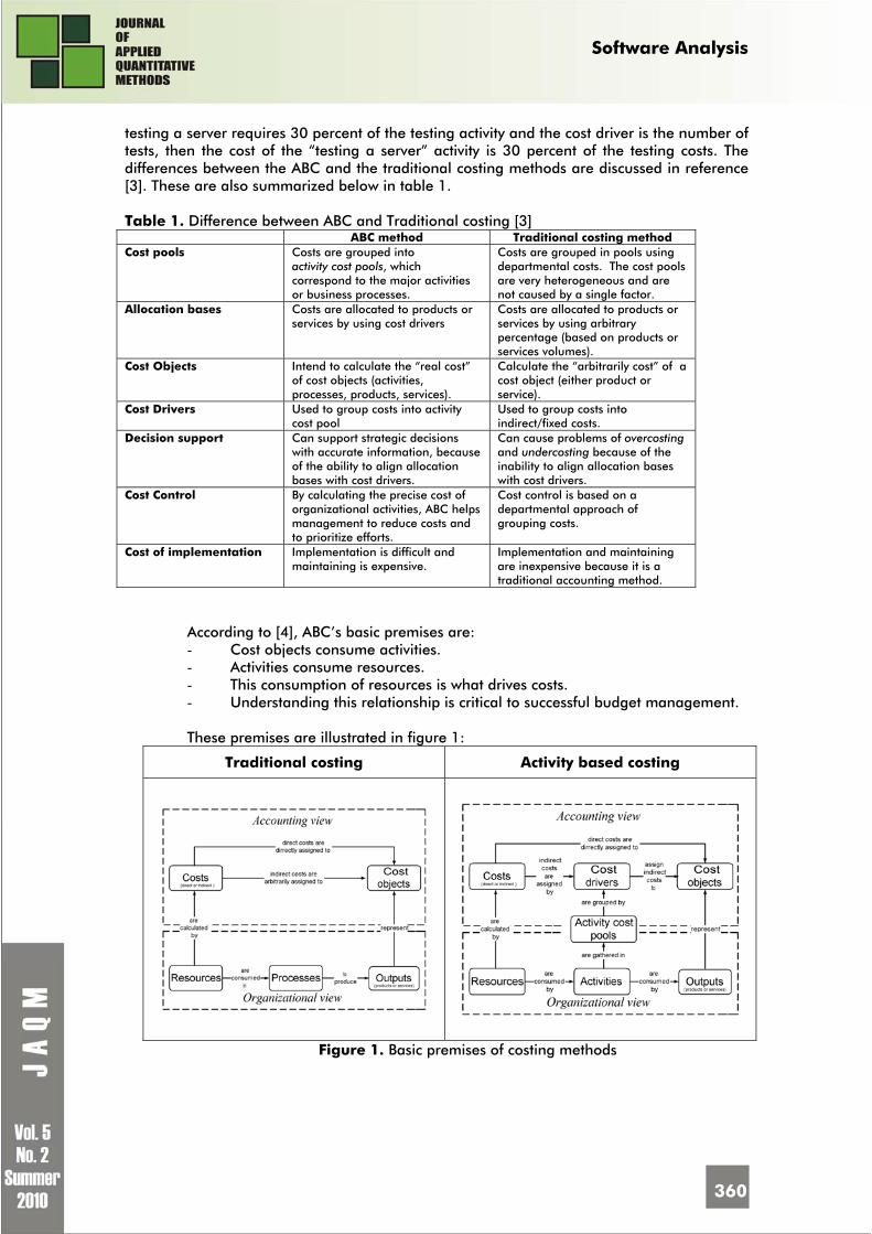
Software Analysis
360
testing a server requires 30 percent of the testing activity and the cost driver is the number of tests, then the cost of the “testing a server” activity is 30 percent of the testing costs. The differences between the ABC and the traditional costing methods are discussed in reference [3]. These are also summarized below in table 1.
Table 1. Difference between ABC and Traditional costing [3] ABC method Traditional costing method Cost pools Costs are grouped into
activity cost pools, which correspond to the major activities or business processes.
Costs are grouped in pools using departmental costs. The cost pools are very heterogeneous and are not caused by a single factor.
Allocation bases Costs are allocated to products or services by using cost drivers
Costs are allocated to products or services by using arbitrary percentage (based on products or services volumes).
Cost Objects Intend to calculate the “real cost” of cost objects (activities, processes, products, services).
Calculate the “arbitrarily cost” of a cost object (either product or service).
Cost Drivers Used to group costs into activity cost pool
Used to group costs into indirect/fixed costs.
Decision support Can support strategic decisions with accurate information, because of the ability to align allocation bases with cost drivers.
Can cause problems of overcosting and undercosting because of the inability to align allocation bases with cost drivers.
Cost Control By calculating the precise cost of organizational activities, ABC helps management to reduce costs and to prioritize efforts.
Cost control is based on a departmental approach of grouping costs.
Cost of implementation Implementation is difficult and maintaining is expensive.
Implementation and maintaining are inexpensive because it is a traditional accounting method.
According to [4], ABC’s basic premises are: - Cost objects consume activities. - Activities consume resources. - This consumption of resources is what drives costs. - Understanding this relationship is critical to successful budget management. These premises are illustrated in figure 1:
Traditional costing Activity based costing
Figure 1. Basic premises of costing methods

Software Analysis
361
The main benefits of Activity-Based Costing method are: - ABC method offers a way for understanding various costs involved and offer information for: analyzing the costs, identify the activities which add value to a product or service and obtaining the benefits. - ABC could improve organization performance, by increasing cost visibility. - ABC could be used as a management tool that provides better allocation of resources. - ABC offers a competitive cost advantage. The main disadvantage of Activity Based Costing is given by the fact that the
implementation is expensive and difficult. However, there are special activity based costing programs, which could be helpful.
4. Results and Discussion
The cost model proposed by the authors of this paper use the ABC method to
identify the cost associated with an output service, for example the “Administration of IT server”.
As a starting point we take into consideration the terms from relation (1), calculated for a precise period of time (i.e. a month or a year), as exemplified in table 2:
Table 2. IT Department budget
Total Costs of IT Department Cost of space 24,000 RON Cost of power 34,500 RON Cost of cooling 9,000 RON Cost of operation, which include: - Salary 36,000 RON - Purchase of new products (hardware and software)
30,000 RON
- Courses for personnel 5,000 RON - Purchase of spare parts for equipments 9,000 RON - Programming 7,000 RON
TOTAL COSTS PER PERIOD 138,000 RON This table shows also the organizational resource consumption for IT department,
in order to produce outputs (products and services). Evidently, the data and information offered by the Table are not enough for
calculating the exact cost of the service called “Administration of IT server”. The first three costs from Table will be allocated to service called “Administration of
IT server”, using parameters like: total area of IT department, area occupied by server, total power consumed by IT department, total power consumed by server, total weight of IT equipment, weight of server .
The cost of space for server is calculated in table 3:
Table 6. Cost of space for server 1. Total cost of space 24,000 RON 2. Area of space occupied with equipments 20 square meters 3. Area of space occupied with server 0.5 square meters 4. Cost of space occupied with the server ( = 1 * 3 / 2 )
600 RON
The cost of power for server is calculated in Table 7:

Software Analysis
362
Table 7. Cost of power for server 1. Total cost of power 34,500 RON 2. Total power of IT equipments 10 KWatts 3. Total power consumed by server 500 Watts 4. Period of time 8,760 hours 5. Total power consumed by IT equipments ( = 2 * 4 )
87,600 KWh
6. Total power consumed by server ( = 3 * 4 )
4,380 KWh
7. Cost of power consumed by server ( = 1 * 6 / 5 )3
1,725 RON
The cost of cooling for server is calculated in Table 8:
Table 8. Cost of cooling the server 1. Total cost of cooling 9,000 RON 2. Total weight of IT equipments 1000 Kg 3. Total weight of server 30 Kg 4. Cost of cooling for server ( = 1 * 3 / 2 )
270 RON
For a precise allocation of the fourth term (cost of operation) to the cost object
“Administration of IT server”, the ABC method is necessary. The steps necessary for applying ABC method are: 1. Identify activities. 2. Identify cost drivers. 3. Group activities into activity cost pools. 4. Determine the cost for each activity pool. 5. Identify outputs. 6. Assign activity costs to outputs. We illustrate this methodology in the following sections. 1. Identify activities In the first step, the main activities of the IT department must be identified and
analyzed. This is the most time-consuming and costly step because it requires a great level of detail. The most common method for identifying IT processes and activities is based on IT employee surveys. The activities are, for example: setup and configuring equipments and programs, service of equipments and programs (maintenance and repairing), developing new programs, supporting the users of the IT systems. The method accuracy depends on the number of activities that are taking into consideration. In table 3 is presented the list of activities used for obtaining the output (service) called “Administration of IT server”.
2. Identify cost drivers In this step, cost drivers are associated with each activity as exemplified in Table 9:
Table 9. Identifying cost drivers Activity Cost driver
Setup and configuring equipments Number of setups Setup and configuring programs Number of setups Service of equipments (maintenance and repairing)
Number of incidents
Service of programs (maintenance and repairing)
Number of incidents
Develop new programs Programming hours Support for users Number of calls

Software Analysis
363
3. Group activities into activity cost pools In this step, similar activities with the same cost driver are gathered together, as is
shown in Table 10:
Table 10. Activity cost pools Activity pool Cost driver
Setup and configuring Number of setups Service Number of incidents Develop new programs Programming hours Support for users Number of calls
4. Determine the cost for each activity pool The cost of each activity cost pool is obtained from the accounting department.
These data is collected in a table format such as the one presented in Table 11 below. Table 11. Identifying cost objects
Activity
Value (cost of activity)
Setup and configuring 24,500 RON Service 19,000 RON Develop new programs 22,500 RON Support for users 21,000 RON
TOTAL 87,000 RON
5. Identify outputs The output is a product or a service. Every output could be a cost object. In this
example, the output is the service called “Administration of IT server”. 6. Assign activity costs to outputs In this step, the cost drivers determined in the previous step are used to assign cost
objects (activity costs) to the output service “Administration of IT server” as presented in Table 12. Table 12. Calculating the cost of Administration of IT server
Cost object
Value (cost of activity)
Number of activities per department
Number of activities
allocated to Administration of IT
server
Cost allocated to Administration of IT
server
Setup and configuring 24,500 RON 15 setups 4 setups 6533,33 RON Service 19,000 RON 18 incidents 5 incidents 5277,78 RON Develop new programs
22,500 RON 160 hours
120 hours 16875 RON
Support for users 21,000 RON 800 calls 98 calls 2572,5 RON Cost of operation for Administration of IT server 31258,61 RON
Finally, all costs presented in relation (1) are allocated to cost object
“Administration of IT server”. So, the precise cost of this service can be calculated as is shown in Table 13: Table 13. Calculating the total cost for output Administration of IT server Cost of space occupied with the server 600 RON Cost of power consumed by server 1,725 RON Cost of cooling for server 270 RON Cost of operation for Administration of IT server 31,258.61 RON TOTAL COST for Administration of IT server 33,853.61 RON

Software Analysis
364
Using this methodology a precise cost for each “output” (product or service) can be calculated based on “the consumption” of each activity and resource.
5. Summary and conclusions The novelty of the approach presented by the authors consist in combining the two
costing methods described above that results in an improved approach for calculating and budgeting the IT activities and ultimately in supporting management decisions.
HP Laboratories offer an exhaustive method for calculating the total cost involved in operating a data center that could be used also for IT department of an organization. However it doesn’t contain any indication about how to assign the indirect costs to products or services. In order to exactly calculate the exact cost of resources consumed for a product or service (to transform indirect costs into direct costs), the method presented above can be applied
The precision of ABC method is increasing proportionally with the number of activities identified. For good results, a number of, at least, 100-150 activities must be considered.
Alternatively, traditional accounting methods could be applied in place of the ABC method; however, due to the way that they allocate the indirect costs, they are not precise enough. Therefore we consider the Activity-Based Costing model as a better alternative to the traditional methods because it uses an allocation model of indirect costs based on activities.
References
1. Chandrakant D. Patel and Amip J. Shahl, Cost Model for Planning, Development and Operation of a Data Center, HP Laboratories Palo Alto, 2005
2. Kaplan, R. S. and Bruns, W. Accounting and Management: A Field Study Perspective, Harvard Business School Press, 1987
3. Granof Michael, H., Platt David, E. and Vaysman, I. Using Activity-Based Costing to Manage More Effectively, University of Texas at Austin, 2000
4. * * * http://www.defenselink.mil/ 5. * * * http://www.valuebasedmanagement.net/
1 Marius MIHUŢ is PhD candidate at Faculty of Economics and Business Administration, Babeş-Bolyai University of Cluj-Napoca. His main research areas include network and information security, IT law and costs. He has published 9 papers focused on multidisciplinary approach of IT security issues. 2 Nicolae TOMAI is full Professor at Faculty of Economics and Business Administration, Babeş-Bolyai University of Cluj-Napoca. His main research areas are: Fundamentals of Computer Science, C#, Computer Networks and Distributed Systems, E-business, Mobile systems His work includes 19 books, 71 scientific papers published, 1 patent, innovation patent 5, active member in 18 research contracts. 3 Although the uptime for an average server is around 99.99 % of total time, during the maintenance and service periods the server actually is powered-on.

Book Review
365
Sabry M. ABD-EL-FATTAH Department of Educational Psychology, Minia University, Minia, Egypt E-mail: [email protected]
Key words: structural equation; modeling; AMOS; Barbara Byrne
Book Review
STRUCTURAL EQUATION MODELING WITH AMOS: BASIC CONCEPTS, APPLICATIONS AND PROGRAMMING
(2nd ed.) by Barbara M. BYRNE,
Routledge/Taylor & Francis, New York
One of the most imperative
statistical and methodological innovations within area of psychology and education over the last few decades concerns the introduction of structural equation modeling (SEM). SEM links regression analysis to factor analysis. A factor model can be specified for the relationships among sets of items tapping the latent variables underlying these items; at the same time, a regression model can be specified for the relationships among these latent variables. One main advantage of SEM over other multivariate approaches is that it reduces the influence of measurement error on these regression estimates, as such errors are already “partialled out” in the factor model. A further advantage is that models can be specified and tested in details; for example, whereas traditional exploratory factor analysis assumes that all items load on all underlying dimensions, in SEM specific factor models can be specified and tested. Yet another advantage is that the fit of a model to the data can be tested and compared to the fit of competing models, thus allowing researchers to see which theoretical notions are supported empirically (Teo & Khine, 2009).

Book Review
366
One of the most popular SEM software is that of James Arbuckle; the AMOS program. It features a sophisticated graphical interface that makes the model specification simple and the analysis output much easier to read. Furthermore, because model specification is so much easier, in my experience, users tend to make much fewer errors in specifying models than using other SEM software with no graphical interface.
Although the user’s manual (Arbuckle, 2009) does a fantastic job in discussing the basic features and operation of AMOS, it falls short in two respects. First, although model specification is easy, users still have to translate their research questions into the right model (or series of models). Second, on a more theoretical level, it is important to realize that model specification is part of the job; SEM comes with a highly structured set of methodological strategies and notions that must be understood before it can be applied effectively.
One of the true virtues of the second edition of Barbara Byrne’s book, Structural Equation Modeling with AMOS, is that it deals quite well with these two issues. According to the Preface "….overall goal is to provide readers with a nonmathematical introduction to basic concepts associated with structural equation modeling (SEM), and to illustrate basic applications of SEM using the AMOS program." All applications in the book were based on the AMOS 17.0 program.
The second edition of the book is different from the first edition in several aspects. First, the number of applications has been expanded to include the testing of: a multitrait-multimethod model, a latent growth curve model, and a second-order model based on categorical data using a Bayesian statistical approach. Second, an update was implemented concerning the automated multi-group approach to test for equivalence. Third, data derived from the use of Likert scaled measures was analyzed using both continuous and categorical approaches. Fourth, there was an update concerning the AMOS text output files which are now imbedded within cell format. Fifth, all applications are based on the graphical mode only of the program. Thus, in contrast to the first edition of this book, example input files for AMOS based on a programming approach (formerly called AMOS Basic) are not included. Finally, all data files used for the applications in this book have been uploaded on a new website: http://www.psypress.com/sem-with-amos/
The book is divided into five major sections. The first section discusses the basics of SEM, and presents a general introduction to model specification in AMOS. The remaining four sections deal with applications of AMOS to exemplary real life data sets drawn from Byrne’s own archives. The second section is devoted to applications involving single-group analyses (i.e., analyses in which data are available for one group only; no across-group comparisons are made). This section addresses simple applications such as testing first- and second-order factor models and “causal” models (i.e., models in which some variables are presumed to affect other variables in the model causally). The third section discusses more complicated multi-group analyses (analyses in which models are compared across different groups; e.g., does the same model apply to boys and girls? can we cross-validate a particular model using data from another group?). The fourth section tackles construct validity via the multitrait-multimethod model and change over time via the latent growth model. The fifth section addresses the analysis of non-normal data using the bootstrap and missing values or incomplete data.
All chapters in these five sections follow the same format. First, a substantive research question is introduced; then the model corresponding to this research question is

Book Review
367
presented and applied to a data set; next the output for this analysis is presented and discussed. Thus, the book can be used as a sort of cookbook; if this is the question you want to address, then this is your model and this is how you should interpret your results. The success of such an approach depends on the range of models considered. That is, by this approach readers are getting familiar with a limited number of models only. Although the readers will be able to modify these models to some degree, they may be more or less helpless when confronted with research questions or data types that require a wholly different approach.
Fortunately, Byrne covers most of the grounds relevant to education and psychology researchers. There is one exception to this general rule. Many psychological theories distinguish between main and moderator (or interaction) effects of the variables included in these models. For example, educational and psychological researchers may examine the effect of pay increase on teachers’ job satisfaction, while acknowledging that these effects may vary as a function of teachers’ educational qualifications. Given the importance of this issue and the fact that specification of interaction effects is not exactly easy in SEM, I would have expected some attention for this issue in this book.
Overall, Byrne’s book is a valuable source to those who seek to analyze their data with SEM techniques because it addresses most of the problems readers will encounter in their own research. The remarkable features including clear style, rich illustrations of a comprehensive range of topics based on real empirical data, and simple-to-follow examples have made this book the first choice by researchers, teachers, students, and other for clearly understandable input and examples on applying SEM with AMOS.
References 1. Teo, T., & Khine, M. S. (Eds.). Structural equation modeling in educational research:
Concepts and applications, Rotterdam, Netherlands: Sense, 2009 2. Arbuckle, J. AMOS 17.0 user’s guide, Crawfordville, FL. Amos Development
Corporation, 2009