Embed Size (px)
Citation preview

Journal of Computational and Applied MathematicsCopyright © 2003 Elsevier B.V. All rights reserved Volume 128, Issues 1-2, Pages 1-467 (1 March 2001)
Display Checked Docs | E-mail Articles | Export Citations View: Citations
1. gfedcFrom finite differences to finite elements: A short history of numerical analysis of partial differential equations, Pages 1-54 Vidar Thomée SummaryPlus | Full Text + Links | PDF (426 K)
2. gfedcOrthogonal spline collocation methods for partial differential equations, Pages 55-82 B. Bialecki and G. Fairweather SummaryPlus | Full Text + Links | PDF (202 K)
3. gfedcSpectral methods for hyperbolic problems, Pages 83-131 D. Gottlieb and J. S. Hesthaven SummaryPlus | Full Text + Links | PDF (387 K)
4. gfedcWavelet methods for PDEs –– some recent developments, Pages 133-185 Wolfgang Dahmen SummaryPlus | Full Text + Links | PDF (385 K)
5. gfedcDevising discontinuous Galerkin methods for non-linear hyperbolic conservation laws, Pages 187-204 Bernardo Cockburn Abstract | PDF (195 K)
6. gfedcAdaptive Galerkin finite element methods for partial differential equations, Pages 205-233 R. Rannacher Abstract | PDF (571 K)
7. gfedcThe p and hp finite element method for problems on thin domains, Pages 235-260 Manil Suri SummaryPlus | Full Text + Links | PDF (304 K)
8. gfedcEfficient preconditioning of the linearized Navier–Stokes equations for incompressible flow, Pages 261-279 David Silvester, Howard Elman, David Kay and Andrew Wathen SummaryPlus | Full Text + Links | PDF (209 K)
9. gfedcA review of algebraic multigrid, Pages 281-309 K. Stüben Abstract | PDF (407 K)
10. gfedcGeometric multigrid with applications to computational fluid dynamics, Pages 311-334 P. Wesseling and C. W. Oosterlee SummaryPlus | Full Text + Links | PDF (159 K)
11. gfedcThe method of subspace corrections, Pages 335-362 Jinchao Xu SummaryPlus | Full Text + Links | PDF (199 K)
Moving finite element, least squares, and finite volume approximations of steady and time-dependent PDEs in
12. gfedcmultidimensions, Pages 363-381 M. J. Baines SummaryPlus | Full Text + Links | PDF (150 K)
13. gfedcAdaptive mesh movement –– the MMPDE approach and its applications, Pages 383-398 Weizhang Huang and Robert D. Russell SummaryPlus | Full Text + Links | PDF (128 K)
14. gfedcThe geometric integration of scale-invariant ordinary and partial differential equations, Pages 399-422 C. J. Budd and M. D. Piggott SummaryPlus | Full Text + Links | PDF (213 K)
15. gfedcA summary of numerical methods for time-dependent advection-dominated partial differential equations, Pages 423-445 Richard E. Ewing and Hong Wang SummaryPlus | Full Text + Links | PDF (170 K)
16. gfedcApproximate factorization for time-dependent partial differential equations, Pages 447-466 P. J. van der Houwen and B. P. Sommeijer SummaryPlus | Full Text + Links | PDF (175 K)
17. gfedcAuthors Index to Volume 128 (2001), Page 467 SummaryPlus | Full Text + Links | PDF (32 K)
18. gfedcContents, Pages vii-viii SummaryPlus | Full Text + Links | PDF (23 K)
19. gfedcNumerical Analysis 2000: Vol. VII: Partial Differential Equations, Pages ix-xi SummaryPlus | Full Text + Links | PDF (42 K)

Volume 128, Numbers 1I2, 1 March 2001
Contents
Preface ix
V. Thome&eFrom finite differences to finite elements. A short history of numerical analysis of partialdifferential equations 1
B. Bialecki and G. FairweatherOrthogonal spline collocation methods for partial differential equations 55
D. Gottlieb and J.S. HesthavenSpectral methods for hyperbolic problems 83
W. DahmenWavelet methods for PDEs N some recent developments 133
B. CockburnDevising discontinuous Galerkin methods for non-linear hyperbolic conservation laws 187
R. RannacherAdaptive Galerkin finite element methods for partial differential equations 205
M. SuriThe p and hp finite element method for problems on thin domains 235
D. Silvester, H. Elman, D. Kay and A. WathenEfficient preconditioning of the linearized Navier}Stokes equations for incompressible flow 261
K. Stu( benA review of algebraic multigrid 281
P. Wesseling and C.W. OosterleeGeometric multigrid with applications to computational fluid dynamics 311
0377-0427/01/$ - see front matter � 2001 Elsevier Science B.V. All rights reserved.PII: S 0 3 7 7 - 0 4 2 7 ( 0 1 ) 0 0 3 5 1 - X

J. XuThe method of subspace corrections 335
M.J. BainesMoving finite element, least squares, and finite volume approximations of steady and time-dependent PDEs in multidimensions 363
W. Huang and R.D. RussellAdaptive mesh movement* the MMPDE approach and its applications 383
C.J. Budd and M.D. PiggottThe geometric integration of scale-invariant ordinary and partial differential equations 399
R.E. Ewing and H. WangA summary of numerical methods for time-dependent advection-dominated partial differentialequations 423
P.J. van der Houwen and B.P. SommeijerApproximate factorization for time-dependent partial differential equations 447
Author Index Volume 128 467
viii Contents
Journal of Computational and Applied Mathematics 128 (2001) ix–xiwww.elsevier.nl/locate/cam
Preface
Numerical Analysis 2000Vol. VII: Partial Di(erential Equations
Over the second half of the 20th century the subject area loosely referred to as numerical analysisof partial di�erential equations (PDEs) has undergone unprecedented development. At its practicalend, the vigorous growth and steady diversi0cation of the 0eld were stimulated by the demand for ac-curate and reliable tools for computational modelling in physical sciences and engineering, and by therapid development of computer hardware and architecture. At the more theoretical end, the analyticalinsight into the underlying stability and accuracy properties of computational algorithms for PDEswas deepened by building upon recent progress in mathematical analysis and in the theory of PDEs.
To embark on a comprehensive review of the 0eld of numerical analysis of partial di(erentialequations within a single volume of this journal would have been an impossible task. Indeed, the 16contributions included here, by some of the foremost world authorities in the subject, represent onlya small sample of the major developments. We hope that these articles will, nevertheless, providethe reader with a stimulating glimpse into this diverse, exciting and important 0eld.
The opening paper by Thom�ee reviews the history of numerical analysis of PDEs, starting with the1928 paper by Courant, Friedrichs and Lewy on the solution of problems of mathematical physicsby means of 0nite di(erences. This excellent survey takes the reader through the development of0nite di(erences for elliptic problems from the 1930s, and the intense study of 0nite di(erencesfor general initial value problems during the 1950s and 1960s. The formulation of the concept ofstability is explored in the Lax equivalence theorem and the Kreiss matrix lemmas. Reference ismade to the introduction of the 0nite element method by structural engineers, and a description isgiven of the subsequent development and mathematical analysis of the 0nite element method withpiecewise polynomial approximating functions. The penultimate section of Thom=ee’s survey dealswith ‘other classes of approximation methods’, and this covers methods such as collocation methods,spectral methods, 0nite volume methods and boundary integral methods. The 0nal section is devotedto numerical linear algebra for elliptic problems.
The next three papers, by Bialecki and Fairweather, Hesthaven and Gottlieb and Dahmen, de-scribe, respectively, spline collocation methods, spectral methods and wavelet methods. The work byBialecki and Fairweather is a comprehensive overview of orthogonal spline collocation from its 0rstappearance to the latest mathematical developments and applications. The emphasis throughout is onproblems in two space dimensions. The paper by Hesthaven and Gottlieb presents a review of Fourierand Chebyshev pseudospectral methods for the solution of hyperbolic PDEs. Particular emphasis isplaced on the treatment of boundaries, stability of time discretisations, treatment of non-smooth solu-
0377-0427/01/$ - see front matter c© 2001 Elsevier Science B.V. All rights reserved.PII: S 0377-0427(00)00508-2

x
tions and multidomain techniques. The paper gives a clear view of the advances that have been madeover the last decade in solving hyperbolic problems by means of spectral methods, but it shows thatmany critical issues remain open. The paper by Dahmen reviews the recent rapid growth in the use ofwavelet methods for PDEs. The author focuses on the use of adaptivity, where signi0cant successeshave recently been achieved. He describes the potential weaknesses of wavelet methods as well as theperceived strengths, thus giving a balanced view that should encourage the study of wavelet methods.
Aspects of 0nite element methods and adaptivity are dealt with in the three papers by Cockburn,Rannacher and Suri. The paper by Cockburn is concerned with the development and analysis ofdiscontinuous Galerkin (DG) 0nite element methods for hyperbolic problems. It reviews the keyproperties of DG methods for nonlinear hyperbolic conservation laws from a novel viewpoint thatstems from the observation that hyperbolic conservation laws are normally arrived at via modelreduction, by elimination of dissipation terms. Rannacher’s paper is a 0rst-rate survey of duality-baseda posteriori error estimation and mesh adaptivity for Galerkin 0nite element approximations of PDEs.The approach is illustrated for simple examples of linear and nonlinear PDEs, including also anoptimal control problem. Several open questions are identi0ed such as the eGcient determination ofthe dual solution, especially in the presence of oscillatory solutions. The paper by Suri is a lucidoverview of the relative merits of the hp and p versions of the 0nite element method over theh version. The work is presented in a non-technical manner by focusing on a class of problemsconcerned with linear elasticity posed on thin domains. This type of problem is of considerablepractical interest and it generates a number of signi0cant theoretical problems.
Iterative methods and multigrid techniques are reviewed in a paper by Silvester, Elman, Kayand Wathen, and in three papers by St&uben, Wesseling and Oosterlee and Xu. The paper bySilvester et al. outlines a new class of robust and eGcient methods for solving linear algebraicsystems that arise in the linearisation and operator splitting of the Navier–Stokes equations. A generalpreconditioning strategy is described that uses a multigrid V -cycle for the scalar convection–di(usionoperator and a multigrid V -cycle for a pressure Poisson operator. This two-stage approach gives riseto a solver that is robust with respect to time-step-variation and for which the convergence rate isindependent of the grid. The paper by StHuben gives a detailed overview of algebraic multigrid. This isa hierarchical and matrix-based approach to the solution of large, sparse, unstructured linear systemsof equations. It may be applied to yield eGcient solvers for elliptic PDEs discretised on unstructuredgrids. The author shows why this is likely to be an active and exciting area of research for severalyears in the new millennium. The paper by Wesseling and Oosterlee reviews geometric multigridmethods, with emphasis on applications in computational Iuid dynamics (CFD). The paper is notan introduction to multigrid: it is more appropriately described as a refresher paper for practitionerswho have some basic knowledge of multigrid methods and CFD. The authors point out that textbookmultigrid eGciency cannot yet be achieved for all CFD problems and that the demands of engineeringapplications are focusing research in interesting new directions. Semi-coarsening, adaptivity andgeneralisation to unstructured grids are becoming more important. The paper by Xu presents anoverview of methods for solving linear algebraic systems based on subspace corrections. The methodis motivated by a discussion of the local behaviour of high-frequency components in the solution ofan elliptic problem. Of novel interest is the demonstration that the method of subspace correctionsis closely related to von Neumann’s method of alternating projections. This raises the question asto whether certain error estimates for alternating directions that are available in the literature maybe used to derive convergence estimates for multigrid and=or domain decomposition methods.
xi
Moving 0nite element methods and moving mesh methods are presented, respectively, in the pa-pers by Baines and Huang and Russell. The paper by Baines reviews recent advances in Galerkinand least-squares methods for solving 0rst- and second-order PDEs with moving nodes in multidi-mensions. The methods use unstructured meshes and they minimise the norm of the residual of thePDE over both the computed solution and the nodal positions. The relationship between the moving0nite element method and L2 least-squares methods is discussed. The paper also describes moving0nite volume and discrete l2 least-squares methods. Huang and Russell review a class of movingmesh algorithms based upon a moving mesh partial di(erential equation (MMPDE). The authorsare leading players in this research area, and the paper is largely a review of their own work indeveloping viable MMPDEs and eGcient solution strategies.
The remaining three papers in this special issue are by Budd and Piggott, Ewing and Wangand van der Houwen and Sommeijer. The paper by Budd and Piggott on geometric integrationis a survey of adaptive methods and scaling invariance for discretisations of ordinary and partialdi(erential equations. The authors have succeeded in presenting a readable account of material thatcombines abstract concepts and practical scienti0c computing. Geometric integration is a new andrapidly growing area which deals with the derivation of numerical methods for di(erential equationsthat incorporate qualitative information in their structure. Qualitative features that may be presentin PDEs might include symmetries, asymptotics, invariants or orderings and the objective is to takethese properties into account in deriving discretisations. The paper by Ewing and Wang gives a briefsummary of numerical methods for advection-dominated PDEs. Models arising in porous mediumIuid Iow are presented to motivate the study of the advection-dominated Iows. The numericalmethods reviewed are applicable not only to porous medium Iow problems but second-order PDEswith dominant hyperbolic behaviour in general. The paper by van der Houwen and Sommeijer dealswith approximate factorisation for time-dependent PDEs. The paper begins with some historical notesand it proceeds to present various approximate factorisation techniques. The objective is to showthat the linear system arising from linearisation and discretisation of the PDE may be solved moreeGciently if the coeGcient matrix is replaced by an approximate factorisation based on splitting.The paper presents a number of new stability results obtained by the group at CWI Amsterdam forthe resulting time integration methods.
We are grateful to the authors who contributed to the Special Issue and to all the referees whoreviewed the submitted papers. We are also grateful to Luc Wuytack for inviting us to edit thisSpecial Issue.
David M. SloanDepartment of Mathematics
University of StrathclydeLivingstone Tower, 26 Richmond street
Glasgow, Scotland, G1 1XH, UKE-mail address: [email protected]
Endre SHuliUniversity of Oxford, Oxford, UK
Stefan VandewalleKatholieke Universiteit Leuven
Leuven, Belgium

Journal of Computational and Applied Mathematics 128 (2001) 1–54www.elsevier.nl/locate/cam
From #nite di$erences to #nite elementsA short history of numerical analysis of partial
di$erential equationsVidar Thom)ee
Department of Mathematics, Chalmers University of Technology, S-412 96 G oteborg, Sweden
Received 30 April 1999; received in revised form 13 September 1999
Abstract
This is an account of the history of numerical analysis of partial di$erential equations, starting with the 1928 paperof Courant, Friedrichs, and Lewy, and proceeding with the development of #rst #nite di$erence and then #nite elementmethods. The emphasis is on mathematical aspects such as stability and convergence analysis. c© 2001 Elsevier ScienceB.V. All rights reserved.
MSC: 01A60; 65-03; 65M10; 65N10; 65M60; 65N30
Keywords: History; Finite di$erence methods; Finite element methods
0. Introduction
This article is an attempt to give a personal account of the development of numerical analysis ofpartial di$erential equations. We begin with the introduction in the 1930s and further development ofthe #nite di$erence method and then describe the subsequent appearence around 1960 and increasingrole of the #nite element method. Even though clearly some ideas may be traced back further, ourstarting point will be the fundamental theoretical paper by Courant, Friedrichs and Lewy (1928)1
on the solution of problems of mathematical physics by means of #nite di$erences. In this papera discrete analogue of Dirichlet’s principle was used to de#ne an approximate solution by meansof the #ve-point approximation of Laplace’s equation, and convergence as the mesh width tendsto zero was established by compactness. A #nite di$erence approximation was also de#ned for the
E-mail address: [email protected] (V. Thom)ee).1 We refer to original work with publication year; we sometimes also quote survey papers and textbooks which are
numbered separately.
0377-0427/01/$ - see front matter c© 2001 Elsevier Science B.V. All rights reserved.PII: S 0377-0427(00)00507-0

2 V. Thom)ee / Journal of Computational and Applied Mathematics 128 (2001) 1–54
wave equation, and the CFL stability condition was shown to be necessary for convergence; againcompactness was used to demonstrate convergence. Since the purpose was to prove existence ofsolutions, no error estimates or convergence rates were derived. With its use of a variational princi-ple for discretization and its discovery of the importance of mesh-ratio conditions in approximationof time-dependent problems this paper points forward and has had a great inEuence on numericalanalysis of partial di$erential equations.
Error bounds for di$erence approximations of elliptic problems were #rst derived by Gerschgorin(1930) whose work was based on a discrete analogue of the maximum principle for Laplace’sequation. This approach was actively pursued through the 1960s by, e.g., Collatz, Motzkin, Wasow,Bramble, and Hubbard, and various approximations of elliptic equations and associated boundaryconditions were analyzed.
For time-dependent problems considerable progress in #nite di$erence methods was made dur-ing the period of, and immediately following, the Second World War, when large-scale practicalapplications became possible with the aid of computers. A major role was played by the work ofvon Neumann, partly reported in O’Brien, Hyman and Kaplan (1951). For parabolic equations ahighlight of the early theory was the important paper by John (1952). For mixed initial–boundaryvalue problems the use of implicit methods was also established in this period by, e.g., Crank andNicolson (1947). The #nite di$erence theory for general initial value problems and parabolic prob-lems then had an intense period of development during the 1950s and 1960s, when the concept ofstability was explored in the Lax equivalence theorem and the Kreiss matrix lemmas, with furthermajor contributions given by Douglas, Lees, Samarskii, Widlund and others. For hyperbolic equa-tions, and particularly for nonlinear conservation laws, the #nite di$erence method has continuedto play a dominating role up until the present time, starting with work by, e.g., Friedrichs, Lax,and Wendro$.
Standard references on #nite di$erence methods are the textbooks of Collatz [12], Forsythe andWasow [14] and Richtmyer and Morton [28].
The idea of using a variational formulation of a boundary value problem for its numerical solutiongoes back to Lord Rayleigh (1894, 1896) and Ritz (1908), see, e.g., Kantorovich and Krylov [21]. InRitz’s approach the approximate solution was sought as a #nite linear combination of functions suchas, for instance, polynomials or trigonometrical polynomials. The use in this context of continuouspiecewise linear approximating functions based on triangulations adapted to the geometry of thedomain was proposed by Courant (1943) in a paper based on an address delivered to the AmericanMathematical Society in 1941. Even though this idea had appeared earlier, also in work by Couranthimself (see BabuLska [4]), this is often thought of as the starting point of the #nite element method,but the further development and analysis of the method would occur much later. The idea to use anorthogonality condition rather than the minimization of a quadratic functional is attributed to Galerkin(1915); its use for time-dependent problems is sometimes referred to as the Faedo–Galerkin method,cf. Faedo (1949), or, when the orthogonality is with respect to a di$erent space, as the Petrov–Galerkin or Bubnov–Galerkin method.
As a computational method the #nite element method originated in the engineering literature,where in the mid 1950s structural engineers had connected the well established framework analysiswith variational methods in continuum mechanics into a discretization method in which a structure isthought of as divided into elements with locally de#ned strains or stresses. Some of the pioneeringwork was done by Turner, Clough, Martin and Topp (1956) and Argyris [1] and the name of

V. Thom)ee / Journal of Computational and Applied Mathematics 128 (2001) 1–54 3
the #nite element method appeared #rst in Clough (1960). The method was later applied to otherclasses of problems in continuum mechanics; a standard reference from the engineering literature isZienkiewicz [43].
Independently of the engineering applications a number of papers appeared in the mathematicalliterature in the mid-1960s which were concerned with the construction and analysis of #nite dif-ference schemes by the Rayleigh–Ritz procedure with piecewise linear approximating functions, by,e.g., Oganesjan (1962, 1966), Friedrichs (1962), C)ea (1964), DemjanoviLc (1964), Feng (1965), andFriedrichs and Keller (1966) (who considered the Neumann problem). Although, in fact, specialcases of the #nite element method, the methods studied were conceived as #nite di$erence methods;they were referred to in the Russian literature as variational di$erence schemes.
In the period following this, the #nite element method with piecewise polynomial approximatingfunctions was analyzed mathematically in work such as Birkho$, Schultz and Varga (1968), inwhich the theory of splines was brought to bear on the development, and Zl)amal (1968), withthe #rst stringent a priori error analysis of more complicated #nite elements. The so called mixed#nite element methods, which are based on variational formulations where, e.g., the solution of anelliptic equation and its gradient appear as separate variables and where the combined variable is asaddle point of a Lagrangian functional, were introduced in Brezzi (1974); such methods have manyapplications in Euid dynamical problems and for higher-order elliptic equations.
More recently, following BabuLska (1976), BabuLska and Rheinboldt (1978), much e$ort has beendevoted to showing a posteriori error bounds which depend only on the data and the computedsolution. Such error bounds can be applied to formulate adaptive algorithms which are of greatimportance in computational practice.
Comprehensive references for the analysis of the #nite element method are BabuLska and Aziz [5],Strang and Fix [34], Ciarlet [11], and Brenner and Scott [8].
Simultaneous with this development other classes of methods have arisen which are related to theabove, and we will sketch four such classes: In a collocation method an approximation is sought in a#nite element space by requiring the di$erential equation to be satis#ed exactly at a #nite number ofcollocation points, rather than by an orthogonality condition. In a spectral method one uses globallyde#ned functions, such as eigenfunctions, rather than piecewise polynomials approximating functions,and the discrete solution may be determined by either orthogonality or collocation. A 4nite volumemethod applies to di$erential equations in divergence form. Integrating over an arbitrary volume andtransforming the integral of the divergence into an integral of a Eux over the boundary, the method isbased on approximating such a boundary integral. In a boundary integral method a boundary valueproblem for a homogeneous elliptic equation in a d-dimensional domain is reduced to an integralequation on its (d − 1)-dimensional boundary, which in turn can be solved by, e.g., the Galerkin#nite element method or by collocation.
An important aspect of numerical analysis of partial di$erential equations is the numerical solu-tion of the #nite linear algebraic systems that are generated by the discrete equations. These are ingeneral very large, but with sparse matrices, which makes iterative methods suitable. The develop-ment of convergence analysis for such methods has parallelled that of the error analysis sketchedabove. In the 1950s and 1960s particular attention was paid to systems associated with #nite dif-ference approximation of positive type of second-order elliptic equations, particularly the #ve-pointscheme, and starting with the Jacobi and Gauss–Seidel methods techniques were developed suchas the Frankel and Young successive overrelaxation and the Peaceman–Rachford (1955) alternating

4 V. Thom)ee / Journal of Computational and Applied Mathematics 128 (2001) 1–54
direction methods, as described in the inEuential book of Varga [39]. In later years systems withpositive-de#nite matrices stemming from #nite element methods have been solved #rst by the conju-gate gradient method proposed by Hestenes and Stiefel (1952), and then making this more e$ectiveby preconditioning. The multigrid method was #rst introduced for #nite di$erence methods in the1960s by Fedorenko and Bahvalov and further developed by Brandt in the 1970s. For #nite elementsthe multigrid method and the associated method of domain decomposition have been and are beingintensely pursued by, e.g., Braess, Hackbusch, Bramble, and Widlund.
Many ideas and techniques are common to the #nite di$erence and the #nite element methods,and in some simple cases they coincide. Nevertheless, with its more systematic use of the variationalapproach, its greater geometric Eexibility, and the way it more easily lends itself to error analysis,the #nite element method has become the dominating approach both among numerical analysts andin applications. The growing need for understanding the partial di$erential equations modeling thephysical problems has seen an increase in the use of mathematical theory and techniques, and has at-tracted the interest of many mathematicians. The computer revolution has made large-scale real-worldproblems accessible to simulation, and in later years the concept of computational mathematics hasemerged with a somewhat broader scope than classical numerical analysis.
Our approach in this survey is to try to illustrate the ideas and concepts that have inEuencedthe development, with as little technicalities as possible, by considering simple model situations.We emphasize the mathematical analysis of the discretization methods, involving stability and errorestimates, rather than modeling and implementation issues. It is not our ambition to present thepresent state of the art but rather to describe the unfolding of the #eld. It is clear that it is notpossible in the limited space available to do justice to all the many important contributions that havebeen made, and we apologize for omissions and inaccuracies; writing a survey such as this one isa humbling experience. In addition to references to papers which we have selected as important inthe development we have quoted a number of books and survey papers where additional and morecomplete and detailed information can be found; for reason of space we have tried to limit thenumber of reference to any individual author.
Our presentation is divided into sections as follows. Section 1: The Courant–Friedrichs–Lewypaper; Section 2: Finite di$erence methods for elliptic problems; Section 3: Finite di$erence methodsfor initial value problems; Section 4: Finite di$erence methods for mixed initial–boundary valueproblems; Section 5: Finite element methods for elliptic problems; Section 6: Finite element methodsfor evolution equations; Section 7: Some other classes of approximation methods; and Section 8:Numerical linear algebra for elliptic problems.
1. The Courant–Friedrichs–Lewy paper
In this seminal paper from 1928 the authors considered di$erence approximations of both theDirichlet problems for a second-order elliptic equation and the biharmonic equation, and of theinitial–boundary value problem for a second-order hyperbolic equation, with a brief comment alsoabout the model heat equation in one space variable. Their purpose was to derive existence results forthe original problem by constructing #nite-dimensional approximations of the solutions, for which theexistence was clear, and then showing convergence as the dimension grows. Although the aim wasnot numerical, the ideas presented have played a fundamental role in numerical analysis. The paper

V. Thom)ee / Journal of Computational and Applied Mathematics 128 (2001) 1–54 5
appears in English translation, together with commentaries by Lax, Widlund, and Parter concerningits inEuence on the subsequent development, see the quotation in references.
The #rst part of the paper treats the Dirichlet problem for Laplace’s equation,
−Ou= 0 in �; with u= g on @�; (1.1)
where �⊂R2 is a domain with smooth boundary @�. Recall that by Dirichlet’s principle the solutionminimizes
∫ ∫� |�’|2 dx over ’ with ’ = g on @�. For a discrete analogue, consider mesh-points
xj = jh; j ∈ Z2, and let �h be the mesh-points in � for which the neighbors xj±e1 ; xj±e2 are in �(e1 = (1; 0); e2 = (0; 1)), and let !h be those with at least one neighbor outside �. For Uj = U (xj)a mesh-function we introduce the forward and backward di$erence quotients
@lUj = (Uj+el − Uj)=h; R@lUj = (Uj − Uj−el)=h; l= 1; 2: (1.2)
By minimizing a sum of terms of the form (@1Uj)2 + (@2Uj)2 one #nds a unique mesh-function Uj
which satis#es
− @1 R@1Uj − @2 R@2Uj = 0 for xj ∈ �h; with Uj = g(xj) on !h; (1.3)
the #rst equation is the well-known #ve-point approximation
4Uj − (Uj+e1 + Uj−e1 + Uj+e2 + Uj−e2) = 0: (1.4)
It is shown by compactness that the solution of (1.3) converges to a solution u of (1.1) when h→0. By the same method it is shown that on compact subsets of � di$erence quotients of U convergeto the corresponding derivatives of u as h → 0. Also included are a brief discussion of discreteGreen’s function representation of the solution of the inhomogeneous equation, of discretization ofthe eigenvalue problem, and of approximation of the solution of the biharmonic equation.
The second part of the paper is devoted to initial value problems for hyperbolic equations. In thiscase, in addition to the mesh-width h, a time step k is introduced and the discrete function valuesUn
j ≈ u(xj; tn), with tn = nk; n ∈ Z+: The authors #rst consider the model wave equation
utt − uxx = 0 for x ∈ R2; t¿0; with u(·; 0); ut(·; 0) given (1.5)
and the approximate problem, with obvious modi#cation of notation (1.2),
@tR@tUn
j − @xR@xUn
j = 0 for j ∈ Z; n¿1; with Unj given for n= 0; 1:
When k = h the equation may also be expressed as Un+1j +Un−1
j −Unj+1−Un
j−1 = 0, and it follows atonce that in this case the discrete solution at (x; t) = (xj; tn) depends only on the initial data in theinterval (x− t; x+ t). For a general time-step k the interval of dependence becomes (x− t=�; x+ t=�),where �= k=h is the mesh-ratio. Since the exact solution depends on data in (x− t; x+ t) it followsthat if �¿ 1, not enough information is used by the scheme, and hence a necessary condition forconvergence of the discrete solution to the exact solution is that �61; this is referred to as theCourant–Friedrichs–Lewy or CFL condition. By an energy argument it is shown that the appropriatesums over the mesh-points of positive quadratic forms in the discrete solution are bounded, andcompactness is used to show convergence as h → 0 when � = k=h=constant 61. The energyargument is a clever discrete analogue of an argument by Friedrichs and Lewy (1926): For thewave equation in (1.5) one may integrate the identity 0 = 2ut(utt − uxx) = (u2t + u2x)t − 2(uxut)x in xto show that
∫R(u
2t + u2x) dx is independent of t, and thus bounded. The case of two spatial variables
is also brieEy discussed.

6 V. Thom)ee / Journal of Computational and Applied Mathematics 128 (2001) 1–54
In an appendix brief discussions are included concerning a #rst-order hyperbolic equation, themodel heat equation in one space variable, and of wave equations with lower-order terms.
2. Finite di�erence methods for elliptic problems
The error analysis of #nite di$erence methods for elliptic problems started with the work ofGerschgorin (1930). In contrast to the treatment in Courant, Friedrichs and Lewy (1928) this workwas based on a discrete version of the maximum principle. To describe this approach we begin withthe model problem
−Ou= f in �; with u= 0 on @�; (2.1)
where we #rst assume � to be the square �=(0; 1)×(0; 1)⊂R2. For a #nite di$erence approximationconsider the mesh-points xj = jh with h= 1=M; j ∈ Z2 and the mesh-function Uj =U (xj). With thenotation (1.2) we replace (2.1) by
− �hUj:=− @1 R@1Uj − @2 R@2Uj = fj for xj ∈ �; Uj = 0 for xj ∈ @�: (2.2)
This problem may be written in matrix form as AU=F , where A is a symmetric (M−1)2×(M−1)2matrix whose elements are 4;−1; or 0, with 0 the most common occurrence, cf. (1.4).
For the analysis one #rst shows a discrete maximum principle: If U is such that −�hUj60 (¿0)in �, then U takes its maximum (minimum) on @�; note that −�hUj60 is equivalent to Uj6(Uj+e1+Uj−e1 + Uj+e2 + Uj−e2)=4. Letting W (x) = 1
2 − |x − x0|2 where x0 = (12 ;12 ) we have W (x)¿ 0 in �,
and applying the discrete maximum principle to the function Vj =±Uj − 14 |�hU |�Wj one concludes
easily that, for any mesh-function U on R�,
|U | R�6|U |@� + C|�hU |�; where |U |S =maxxj∈S|Uj|:
Noting that the error zj = Uj − u(xj) satis#es
− �hzj = fj + �hu(xj) = (�h −O)u(xj) = !j; with |!j|6Ch2‖u‖C4 ; (2.3)
one #nds, since zj = 0 on @�, that
|U − u| R� = |z| R�6C|!|�6Ch2‖u‖C4 :
The above analysis uses the fact that all neighbors xj±el of the interior mesh-points xj ∈ � areeither interior mesh-points or belong to @�. When the boundary is curved, however, there will bemesh-points in � which have neighbors outside R�. If for such a mesh-point x = xj we take a pointbh;x ∈ @� with |bh;x − x|6h and set Uj = u(bh;x) = 0, then it follows from Gerschgorin, loc. cit.,that |U − u| R�6Ch‖u‖C3 . To retain second-order accuracy Collatz (1933) proposed to use linearinterpolation near the boundary: Assuming for simplicity that � is a convex plane domain withsmooth boundary, we denote by �h the mesh-points xj ∈ �h that are truly interior in the sensethat all four neighbors of xj are in R�. (For the above case of a square, �h simply consists of allmesh-points in �.) Let now !h be the mesh-points in � that are not in �h. For xj ∈ !h we maythen #nd a neighbor y= xi ∈ �h ∪ !h such that the line through x and y cuts @� at a point Rx whichis not a mesh-point. We denote by R!h the set of points Rx ∈ @� thus associated with the points of!h, and de#ne for x = xj ∈ !h the error in the linear interpolant
‘huj:=u(xj)− &u(xi)− (1− &)u( Rx); where &= '=(1 + ')6 12 if |x − Rx|= 'h:
V. Thom)ee / Journal of Computational and Applied Mathematics 128 (2001) 1–54 7
As u= 0 on @� we now pose the problem
−�hUj = fj in �h; ‘hUj = 0 in !h; U ( Rx) = 0 on R!h
and since &6 12 it is not diTcult to see that
|U |�h∪!h6C(|U | R!h + |‘hU |!h + |�hU |�): (2.4)
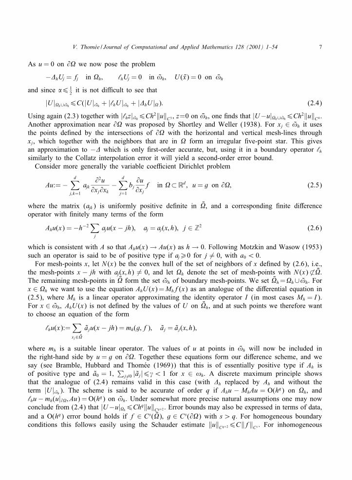
Using again (2.3) together with |‘hz|!h6Ch2‖u‖C3 ; z=0 on R!h, one #nds that |U−u|�h∪!h6Ch2‖u‖C4 .Another approximation near @� was proposed by Shortley and Weller (1938). For xj ∈ !h it usesthe points de#ned by the intersections of @� with the horizontal and vertical mesh-lines throughxj, which together with the neighbors that are in � form an irregular #ve-point star. This givesan approximation to −� which is only #rst-order accurate, but, using it in a boundary operator ‘hsimilarly to the Collatz interpolation error it will yield a second-order error bound.
Consider more generally the variable coeTcient Dirichlet problem
Au:=−d∑
j; k=1
ajk@2u
@xj@xk−
d∑j=1
bj@u@xj
f in �⊂Rd; u= g on @�; (2.5)
where the matrix (ajk) is uniformly positive de#nite in R�, and a corresponding #nite di$erenceoperator with #nitely many terms of the form
Ahu(x) =−h−2∑j
aju(x − jh); aj = aj(x; h); j ∈ Z2 (2.6)
which is consistent with A so that Ahu(x)→ Au(x) as h→ 0. Following Motzkin and Wasow (1953)such an operator is said to be of positive type if aj¿0 for j �= 0, with a0 ¡ 0.
For mesh-points x, let N (x) be the convex hull of the set of neighbors of x de#ned by (2.6), i.e.,the mesh-points x − jh with aj(x; h) �= 0, and let �h denote the set of mesh-points with N (x) �⊂ R�.The remaining mesh-points in R� form the set !h of boundary mesh-points. We set R�h=�h∪ !h. Forx ∈ �h we want to use the equation AhU (x)=Mhf(x) as an analogue of the di$erential equation in(2.5), where Mh is a linear operator approximating the identity operator I (in most cases Mh = I).For x ∈ !h; AhU (x) is not de#ned by the values of U on R�h, and at such points we therefore wantto choose an equation of the form
‘hu(x):=∑xj∈ R�
aju(x − jh) = mh(g; f); aj = aj(x; h);
where mh is a suitable linear operator. The values of u at points in R!h will now be included inthe right-hand side by u = g on @�. Together these equations form our di$erence scheme, and wesay (see Bramble, Hubbard and Thom)ee (1969)) that this is of essentially positive type if Ah isof positive type and a0 = 1;
∑j �=0 |aj|6'¡ 1 for x ∈ !h. A discrete maximum principle shows
that the analogue of (2.4) remains valid in this case (with �h replaced by Ah and without theterm |U | R!h). The scheme is said to be accurate of order q if Ahu − MhAu = O(hq) on �h, and‘hu−mh(u|@�; Au) = O(hq) on !h. Under somewhat more precise natural assumptions one may nowconclude from (2.4) that |U−u|�h6Chq‖u‖Cq+2 . Error bounds may also be expressed in terms of data,and a O(hq) error bound holds if f ∈ Cs( R�); g ∈ Cs(@�) with s¿q. For homogeneous boundaryconditions this follows easily using the Schauder estimate ‖u‖Cq+26C‖f‖Cs . For inhomogeneous

8 V. Thom)ee / Journal of Computational and Applied Mathematics 128 (2001) 1–54
boundary conditions a more precise analysis may be based on a representation using a nonnegativediscrete Green’s function Gjl = G(xj; xl),
Uj = hd∑xl∈�h
GjlAhUl +∑xl∈!h
GjlUl for xj ∈ R�h;
where hd∑xl∈�h
Gjl6C and∑
xl∈!hGjl61, and where also a discrete analogue of the estimate∫
01G(x; y) ds6C1 for the continuous problem holds, where 01 = {y ∈ �; dist(y; @�) = 1}. The
latter is related to the important observation by Bahvalov (1959) that the regularity demands onthe solution u of the continuous problem can be relaxed in some cases by essentially two deriva-tives at the boundary without loosing the convergence rate. For less regular data one can obtaincorrespondingly weaker convergence estimates: When f ∈ Cs( R�); g ∈ Cs(@�) with 06s¡q; O(hs)order convergence may be shown by interpolation between Cs-spaces. The regularity demands off may be further relaxed by choosing for Mh an averaging operator, see Tikhonov and Samarskii(1961); this paper also demonstrated how to construct #nite di$erence approximations of ellipticequations with discontinuous coeTcients by taking local harmonic averages. When the boundaryitself is nonsmooth the exact solution may have singularities which make the above results not ap-plicable. Laasonen (1957) showed that the presence of a corner with an accute inner angle doesnot a$ect the rate of convergence but if the angle is 2& with &¿ 1 he shows the weaker estimateO(h1=&−3) for any 3¿ 0.
As an example of an operator of the form (2.6), consider the nine-point formula
−�(9)h u(x) = 1
6 h−2
20 u(x)− 4
∑|j|=1
u(x − jh)−∑
|j1|=|j2|=1
u(x − jh)
:
With Mhf=f+ 112h
2�hf one #nds �(9)h u+MhOu=O(h4) and Bramble and Hubbard (1962) showed
that the operator ‘h can be chosen so that the corresponding scheme is of essentially positive typeand accurate of order q=4. Further, Bramble and Hubbard (1963) constructed second-order accurateschemes of essentially positive type in the case of a general A (d= 2), also with mixed derivativeterms. Here the neighbors of x may be several mesh-widths away from x. Related results were alsoobtained in special cases by Wasow (1952), Laasonen (1958), and Volkov (1966), see also Bramble,Hubbard and Thom)ee (1969).
We shall now turn to some schemes that approximate elliptic equations containing mixed deriva-tives but are not generally of essentially positive type. Assume now that A is in divergence form,A=−∑d
i; k=1(@=@xi)(aik@u=@xk). To our above notation @i; R@i of (1.2) we add the symmetric di$erencequotient @i = (@i + R@i)=2 and set, with a(h)ik = aik(x + 1
2 hei),
A(1)h u=−
∑i; k
R@i(a(h)ik @ku); A(2)
h u=−∑
i
R@i(a(h)ii @iu)−
∑i �=k
@i(aik @ku):
These operators are obviously consistent with A and second-order accurate. Except in special casesthe A(l)
h are not of positive type and the above analysis does not apply. Instead one may use energyarguments to derive error estimates in discrete l2-norms, see Thom)ee (1964). For x ∈ !h let asabove bh;x ∈ @�, and consider the discrete Dirichlet problem
AhU = f on �h; U = g(bh;x) on !h; with Ah = A(1)h or A(2)
h : (2.7)

V. Thom)ee / Journal of Computational and Applied Mathematics 128 (2001) 1–54 9
With Dh the mesh-functions which vanish outside �h, we de#ne for U; V ∈ Dh
(U; V ) = hd∑j
Uj Vj; ‖U‖= (U;U )1=2; and ‖U‖1 = ‖U‖+d∑
j=1
‖@iU‖:
By summation by parts one easily derives that ‖V‖216C(AhV; V ) for V ∈ Dh; and this shows atonce the uniqueness and hence the existence of a solution of (2.7). When !h⊂ @�, application toU − u, using the second-order accuracy of Ah shows that ‖U − u‖16C(u)h2: When !h �⊂@�, h2 hasto be replaced by
√h, but with ‖·‖′1 a slightly weaker norm it was shown in Bramble, Kellogg and
Thom)ee (1968) that ‖U − u‖6‖U − u‖′16C(u)h.Consider now a constant coeTcient #nite di$erence operator of the form (2.6), which is consistent
with A of (2.5). Introducing the symbol of Ah, the trigonometric polynomial p(5) =∑
j ajeij5, we
say that Ah is elliptic if p(5) �= 0 for |5l|6�; l = 1; 2; 5 �= 0: For the #ve-point operator −�h
we have p(5) = 4 − 2 cos 51 − 2 cos 52 and −�h is thus elliptic. For such operators Ah we havethe following interior estimate by Thom)ee and Westergren (1968). Set ‖U‖S = (hd∑
xj∈S U2j )
1=2 and
‖U‖k; S =(∑
|&|6k ‖@&hU‖2S
)1=2where @&
h=@&11 · · · @&d
d ; |&|=&1+ · · ·+&d; and let R�0⊂�1⊂ R�1⊂�. Thenfor any & and h small we have
|@&hU |�06C(‖AhU‖l;�1
+ ‖U‖�1) if l¿|&|+ [d=2]− 1:
Thus, the #nite di$erence quotients of the solution of the equation AhU =f may be bounded in �0
by the di$erence quotients of f in a slightly larger domain �1 plus a discrete l2-norm of U in �1.Assuming u is a solution of (2.1) this may be used to show that if Ah is accurate of order q andQh is a #nite di$erence operator which approximates the di$erential operator Q to order q, then
|QhU − Qu|�06C(u)hq + C‖U − u‖�1: (2.8)
Thus, if we already know that U −u is of order O(hq) in the l2-norm, then Qhu−Qu is of the sameorder in maximum norm in the interior of the domain.
Finite di$erence approximations for elliptic equations of higher order were studied by, e.g., Saulev(1957); the work in Thom)ee (1964) concerns also such equations.
3. Finite di�erence methods for initial value problems
In this section we sketch the development of the stability and convergence theory for #nite dif-ference methods applied to pure initial value problems. We #rst consider linear constant coeTcientevolution equations and then specialize to parabolic and hyperbolic equations.
We begin with the initial value problem for a general linear constant coeTcient scalar equation
ut = P(D)u for x ∈ Rd; t ¿ 0; u(·; 0) = v; where P(5) =∑
|&|6M
P&5& (3.1)
with u= u(x; t); v = v(x); 5& = 5&11 · · · 5&d
d ; and D = (@=@x1; : : : ; @=@xd): Such an initial value problemis said to be well-posed if it has a unique solution that depends continuously on the initial data, insome sense that has to be speci#ed. For example, the one-dimensional wave equation ut = :ux has

10 V. Thom)ee / Journal of Computational and Applied Mathematics 128 (2001) 1–54
the unique solution u(x; t)= v(x+ :t) and since ‖u(·; t)‖Lp= ‖v‖Lp
, this problem is well posed in Lp
for 16p6∞. Similarly, for the heat equation ut = uxx we have
u(x; t) =1√4�t
∫ ∞
−∞e−(x−y)2=4tv(y) dy
and ‖u(·; t)‖Lp6‖v‖Lp
; 16p6∞. More precisely, (3.1) is well-posed in Lp if P(D) generates asemigroup E(t) = etP(D) in Lp which grows at most exponentially, so that the solution u(t) = E(t)vsatis#es ‖u(t)‖Lp
6Ce=t‖v‖Lpfor t¿0, for some =. For p = 2, which is the case we will con-
centrate on #rst, we see by Fourier transformation and Parseval’s relation that this is equivalentto
|etP(i5)|6Ce=t ; ∀5 ∈ Rd; t ¿ 0; (3.2)
or ReP(i5)6= for 5 ∈ Rd; if only the highest-order terms are present in P(D), this is equivalentto ReP(i5)60 for 5 ∈ Rd, in which case (3.2) holds with ==0, so that E(t) is uniformly boundedin L2 for t¿0. In the above examples P(i5) = i:5 and P(i5) =−52, respectively, and = = 0.
Generalizing to systems of the form (3.1) with u and v N -vectors and the P& N ×N matrices, thecondition for well-posedness in L2 is again (3.2) where now | · | denotes any matrix norm. Here itis clear that a necessary condition for (3.2) is that Re �j(5)6= for 5 ∈ Rd, for any eigenvalue �j(5)of P(i5), and if P(i5) is a normal matrix this is also suTcient. Necessary and suTcient conditionsfor (3.2) were given by Kreiss (1959b), and depend on the following lemma. Here, for any N ×Nmatrix A with eigenvalues {�j}Nj=1 we set >(A)=maxj Re �j and ReA=(A+A∗)=2, where A∗ is theadjoint matrix. For Hermitian matrices A6B means Au ·u6Bu ·u for all u ∈ RN . With this notation,(3.2) holds if and only if the set F= {P(i5)− =; 5 ∈ Rd} satis#es the conditions of the followinglemma:
Let F be a set of N × N matrices. Then the following conditions are equivalent:(i) |etA|6C for A ∈F; t¿0; for some C ¿ 0;(ii) >(A)60 and Re (z |R(A; z)|)6C for A ∈F; Re z¿ 0; for some C ¿ 0;(iii) >(A)60 for A ∈ F and there exist C1 and C2 and for each A ∈ F a matrix S = S(A)
such that max(|S|; |S−1|)6C1 and such that SAS−1 = B = (bjk) is a triangular matrix witho8-diagonal elements satisfying |bjk |6C2 min(|Re �j|; |Re �k |) where �j = bjj;
(iv) Let 06'¡ 1. There exists C ¿ 0 such that for each A ∈ F there is a Hermitian matrixH = H (A) with C−1I6H6CI and Re (HA)6'>(A)H60.
Equations of higher order in the time variable such as the wave equation utt = uxx may be writtenin system form (3.1) by introducing the successive time derivatives of u as dependent variables, andis therefore covered by the above discussion.
For the approximate solution of the initial value problem (3.1), let h and k be (small) positivenumbers. We want to approximate the solution at time level tn = nk by Un for n¿0 where U 0 = vand Un+1 = EkUn for n¿0, and where Ek is an operator of the form
Ekv(x) =∑j
aj(h)v(x − jh); �= k=hM = constant (3.3)
with summation over a #nite set of multi-indices j = (j1; : : : ; jd) ∈ Zd; such operators are calledexplicit. The purpose is to choose Ek so that En
k v approximates u(tn)=E(tn)v=E(k)nv. In numericalapplications we would apply (3.3) only for x=xl=lh; l ∈ Zd; but for convenience in the analysis we
V. Thom)ee / Journal of Computational and Applied Mathematics 128 (2001) 1–54 11
shall think of Ekv as de#ned for all x. As an example, for the heat equation ut=uxx the simplest suchoperator is obtained by replacing derivatives by #nite di$erence quotients, @tUn
j = @xR@xUn: Solving
for Un+1 we see that this de#nes Ekv(x) = �v(x+ h) + (1− 2�)v(x) + �v(x− h), �= k=h2. We shallconsider further examples below.
We say that Ek is consistent with (3.1) if u(x; t+k)=Eku(x; t)+o(k) when k → 0, for suTcientlysmooth solutions u(x; t) of (3.1), and accurate of order r if the term o(k) may be replaced bykO(hr). By Taylor series expansion around (x; t) these conditions are seen to be equivalent toalgebraic conditions between the coeTcients aj(h). In our above example, u(x; t + k) − Eku(x; t) =kut + 1
2k2utt − �h2uxx − 1
12�h4uxxxx = kO(h2) when ut = uxx, so that r = 2.
For the purpose of showing convergence of Enk v to E(tn)v and to derive an error bound one needs
some stability property of the operator Enk : This operator is said to be stable in L2 if for any T ¿ 0
there are constants C and = such that ‖Enk v‖6Ce=nk‖v‖ for v ∈ L2; n¿0; where ‖·‖ = ‖·‖L2
. Ifthis holds, and if (3.1) is well posed in L2 and Ek is accurate of order r, then it follows from theidentity En
k − E(tn) =∑n−1
j=0 En−1−jk (Ek − E(k))E(tj) that, with ‖·‖s = ‖·‖Hs(Rd),
‖(Enk − E(tn))v‖6C
n−1∑j=0
khr‖E(tj)v‖M+r6CT hr‖v‖M+r for tn6T; (3.4)
where we have also used the fact that spatial derivatives commute with E(t).The suTciency of stability for convergence of the solution of the discrete problem to the solution
of the continuous initial value problem was shown in particular cases in many places, e.g., Courant,Friedrichs and Lewy (1928), O’Brien, Hyman and Kaplan (1951), Douglas (1956). It was observedby Lax and Richtmyer (1959) that stability is actually a necessary condition for convergence tohold for all v∈L2; the general Banach space formulation of stability as a necessary and suTcientcondition for convergence is known as the Lax equivalence theorem, see Richtmyer and Morton[28]. We note that for individual, suTciently regular v convergence may hold without stability; foran early interesting example with analytic initial data and highly unstable di$erence operator, seeDahlquist (1954). Without stability, however, roundo$ errors will then overshadow the theoreticalsolution in actual computation.
We shall see that the characterization of stability of #nite di$erence operators (3.3) is parallel tothat of well-posedness of (3.1). Introducing the trigonometric polynomial Ek(5) =
∑j aj(h)e
ijh5; thesymbol of Ek , Fourier transformation shows that Ek is stable in L2 if and only if, cf. (3.2),
|Ek(5)n|6Ce=nk ; ∀5 ∈ Rd; n¿0:
In the scalar case this is equivalent to |Ek(5)|61 + Ck for 5 ∈ Rd and small k, or |Ek(5)|61for 5 ∈ Rd when the coeTcients of Ek are independent of h, as is normally the case when nolower-order terms occur in P(D). For our above example Ek(5) = 1 − 2� + 2� cos h5 and stabil-ity holds if and only if � = k=h26 1
2 . For the equation ut = :ux and the scheme @tUnj = @xU n
j
we have Ek(5) = 1 + i:� sin h5 and this method is therefore seen to be unstable for any choiceof �= k=h.Necessary for stability in the matrix case is the von Neumann condition
:(Ek(5))61 + Ck; ∀5 ∈ Rd; (3.5)
where :(A)=maxj|�j| is the spectral radius of A, and for normal matrices Ek(5) this is also suTcient.This covers the scalar case discussed above. Necessary and suTcient conditions are given in the

12 V. Thom)ee / Journal of Computational and Applied Mathematics 128 (2001) 1–54
following discrete version of the above Kreiss matrix lemma, see Kreiss (1962), where we denote|u|H = (Hu; u)1=2 and |A|H = supu �=0|Au|H =|u|H for H positive de#nite:
Let F be a set of N × N matrices. Then the following conditions are equivalent:(i) |An|6C for A ∈F; n¿0; for some C ¿ 0;(ii) :(A)61 and (|z| − 1)|R(A; z)|6C for A ∈F; |z|¿ 1; with C ¿ 0;(iii) :(A)61 for A ∈ F and there are C1 and C2 and for each A ∈ F a matrix S = S(A) such
that max(|S|; |S−1|)6C1 and such that SAS−1 = (bjk) is triangular with o8-diagonal elementssatisfying |bjk |6C2 min(1− |�j|; 1− |�k |) where �j = bjj;
(iv) let 06'¡ 1. There exists C ¿ 0 and for each A ∈ F a Hermitian matrix H = H (A) withC−1I6H6CI and |A|H61− '+ ':(A):
Application shows that if Ek is stable in L2, then there is a = such that F={e−=kEk(5); k6k0; 5 ∈Rd} satis#es conditions (i)–(iv). On the other hand, if one of these conditions holds for some =,then Ek is stable in L2.Other related suTcient conditions were given in, e.g., Kato (1960), where it was shown that if
the range of an N ×N matrix is in the unit disc, i.e., if |Av · v|61 for |v|61, then |Anv · v|61, andhence, by taking real and imaginary parts, |An|62 for n¿1.Using the above characterizations one can show that a necessary and suTcient condition for the
existence of an L2-stable operator which is consistent with (3.1) is that (3.1) is well-posed in L2,see Kreiss (1959a). It was also proved by Wendro$ (1968) that for initial value problems whichare well-posed in L2 one may construct L2-stable di$erence operators with arbitrarily high-order ofaccuracy.
It may be shown that von Neumann’s condition (3.5) is equivalent to growth of at most polynomialorder of the solution operator in L2, or ‖En
k v‖L26Cnq‖v‖L2
for tn6T , for some q¿0. This was usedby Forsythe and Wasow [14] and Ryabenkii and Filippov [29] as a de#nition of stability.
For variable coeTcients it was shown by Strang (1965) that if the initial-value problem for theequation ut=
∑|&|6M P&(x)D&u is well-posed in L2, then the one for the equation without lower-order
terms and with coeTcients #xed at x ∈ Rd is also well-posed, and a similar statement holds forthe stability of the #nite di$erence scheme Ekv(x) =
∑j aj(x; h)v(x − jh). However, Kreiss (1962)
showed that well-posedness and stability with frozen coeTcients is neither necessary nor suTcientfor well-posedness and stability of a general variable coeTcient problem. We shall return below tovariable coeTcients for parabolic and hyperbolic equations.
We now consider the special case when system (3.1) is parabolic, and begin by quoting thefundamental paper of John (1952) in which maximum-norm stability was shown for #nite di$erenceschemes for second-order parabolic equations in one space variable. For simplicity, we restrict ourpresentation to the model problem
ut = uxx for x ∈ R; t ¿ 0; with u(·; 0) = v in R (3.6)
and a corresponding #nite di$erence approximation of the form (3.3) with aj(h)= aj independent ofh. Setting a(5) =
∑j aje
−ij5 = Ek(h−15) one may write
Un(x) =∑j
anjv(x − jh); where anj =12�
∫ �
−�e−ij5a(5)n d5: (3.7)
Here the von Neumann condition reads |a(5)|61, and is necessary and suTcient for stability in L2.To show maximum-norm stability we need to estimate the anj in (3.7). It is easily seen that if the
V. Thom)ee / Journal of Computational and Applied Mathematics 128 (2001) 1–54 13
di$erence scheme is consistent with (3.6) then a(5)= e−�52 + o(52) as 5→ 0; and if we assume that|a(5)|¡ 1 for 0¡ |5|6� it follows that
|a(5)|6e−c52 for |5|6�; with c¿ 0: (3.8)
One then #nds at once from (3.7) that |anj|6Cn−1=2; and integration by parts twice, using |a′(5)|6C|5|,shows |anj|6Cn1=2j−2: Thus∑
j
|anj|6C∑
j6n1=2
n−1=2 +∑
j¿n1=2
n1=2j−26C;
so that ‖Un‖∞6C‖v‖∞ by (3.7) where ‖·‖∞=‖·‖L∞ . We remark that for our simple example abovewe have |Ekv(x)|6(�+ |1− 2�|+ �) ‖v‖∞ = ‖v‖∞ for �6 1
2 , which trivially yields maximum-normstability.
In the general constant coeTcient case system (3.1) is said to be parabolic in Petrowski’s senseif >(P(5))6− 1|5|M +C for 5 ∈ Rd, and using (iii) of the Kreiss lemma one shows easily that thecorresponding initial value problem is well-posed in L2. For well-posedness in L∞ we may write
u(x; t) = (E(t)v)(x) =∫Rd
G(x − y; t)v(y) dy
where, cf., e.g., [15], with D& = D&x ,
|D&G(x; t)|6CT t−(|&|+d)=Me(−1(|x|M =t)1=(M−1)) for 0¡t6T: (3.9)
This implies that ‖D&u(·; t)‖∞6Ct−|&|=M‖v‖∞, so that the solution, in addition to being bounded,is smooth for positive time even if the initial data are only bounded. Consider now a di$erenceoperator of the form (3.3) which is consistent with (3.1). Generalizing from (3.8) we de#ne thisoperator to be parabolic in the sense of John if, for some positive 1 and C,
:(Ek(h−15))6e−1|5|M + Ck; for 5 ∈ Q = {5; |5j|6�; j = 1; : : : ; d};such schemes always exist when (3.1) is parabolic in Petrowski’s sense. Extending the results ofJohn (1952) to this situation Aronson (1963) and Widlund (1966) showed that if we write Un(x)=En
k v(x)=∑
j anj(h)v(x− jh); then, denoting di$erence quotients corresponding to D& by @&h, we have,
cf. (3.9),
|@&hanj(h)|6Chdt−(|&|+d)=M
n e(−c(|j|M =n)1=(M−1)) for tn6T;
which implies that ‖@&hE
nk v‖∞6Ct−|&|=M
n ‖v‖∞. In the work quoted also multistep methods and variablecoeTcients were treated.
From estimates of these types follow also convergence estimates such as, if D&h is a di$erence
operator consistent with D& and accurate of order r,
‖D&hU
n − D&u(tn)‖∞6Chr‖v‖Wr+|&|∞
for tn6T:
Note in the convergence estimate for &= 0 that, as a result of the smoothing property for parabolicequations, less regularity is required of initial data than for the general well-posed initial valueproblem, cf. (3.4). For even less regular initial data lower convergence rates have to be expected;by interpolation between the Ws
∞ spaces one may show (see Peetre and Thom)ee (1967)), e.g.,
‖Un − u(tn)‖∞6Chs‖v‖Ws∞for 06s6r; tn6T:

14 V. Thom)ee / Journal of Computational and Applied Mathematics 128 (2001) 1–54
We remark that for nonsmooth initial data v it is possible to make a preliminary smoothing of v torecover full accuracy for t bounded away from zero: It was shown in Kreiss, Thom)ee and Widlund(1970) that there exists a smoothing operator of the form Mhv=Dh ∗ v, where Dh(x) = h−dD(h−1x),with D an appropriate function, such that if Mhv is chosen as initial data for the di$erence scheme,then
‖Un − u(tn)‖∞ = ‖EnhMhv− E(tn)v‖∞6Chrt−r=M
n ‖v‖∞:Let us also note that from a known convergence rate for the di$erence scheme for #xed initial data
v conclusions may be drawn about the regularity of v. For example, under the above assumptions,assume that for some p; s with 16p6∞; 0¡s6r, we know that ‖Un − u(tn)‖Lp
6Chs for tn6T .Then v belongs to the Besov space Bs;∞
p (≈ Wsp ), and, if s¿ r then v=0. Such inverse results were
given in, e.g., Hedstrom (1968), LWofstrWom (1970), and Thom)ee and Wahlbin (1974).We now turn our attention to hyperbolic equations, and consider #rst systems with constant real
coeTcients
ut =d∑
j=1
Ajuxj for t ¿ 0; with u(0) = v: (3.10)
Such a system is said to be strongly hyperbolic if it is well-posed in L2, cf. Strang (1967). WithP(5) =
∑dj=1 Aj5j this holds if and only if for each 5 ∈ Rd there exists a nonsingular matrix S(5),
uniformly bounded together with its inverse, such that S(5)P(5)S(5)−1 is a diagonal matrix withreal elements. When the Aj are symmetric this holds with S(5) orthogonal; the system is then saidto be symmetric hyperbolic. The condition is also satis#ed when the eigenvalues of P(5) are realand distinct for 5 �= 0; in this case the system is called strictly hyperbolic.
One important feature of hyperbolic systems is that the value u(x; t) of the solution at (x; t) onlydepends on the initial values on a compact set K(x; t), the smallest closed set such that u(x; t) = 0when v vanishes in a neighborhood of K(x; t). The convex hull of K(x; t) may be described in termsof P(5): if K = K(0; 1) we have for its support function F(5) = supx∈K x5= �max(P(5)).
Consider now the system (3.10) and a corresponding #nite di$erence operator of the form (3.3)(with M = 1). Here we introduce the domain of dependence K(x; t) of Ek as the smallest closedset such that En
k v(x) = 0 for all n; k with nk = t when v vanishes in a neighborhood of K(x; t).Corresponding to the above the support function of K(x; t) satis#es F(5) = �−1maxaj �=0 j5: Sinceclearly convergence, and hence stability, demands that K = K(0; 1) contains the continuous do-main of dependence K = K(0; 1) it is necessary for stability that �max(P(5))6�−1maxaj �=0 j5; this isthe CFL-condition, cf. Section 1. In particular, minaj �=0 jl6��min(Al)6��max(Al)6maxaj �=0 jl: For theequation ut = :ux and a di$erence operator of the form (3.3) using only j = −1; 0; 1, this means�|:|61: In this case u(0; 1)= v(:) so that K = {:}, and the condition is thus : ∈ K = [− �−1; �−1]:We shall now give some suTcient conditions for stability. We #rst quote from Friedrichs (1954)
that if aj are symmetric and positive semide#nite, with∑
j aj = I , then |Ek(h−15)|= |∑j ajeij5|61 so
that the scheme is L2-stable. As an example, the #rst order accurate Friedrichs operator
Ekv(x) =12
d∑j=1
((d−1I + �Aj)v(x + hej) + (d−1I − �Aj)v(x − hej)) (3.11)
is L2-stable if 0¡�6(d:(Aj))−1. It was observed by Lax (1961) that this criterion is of limitedvalue in applications because it cannot in general be combined with accuracy higher than #rst order.
V. Thom)ee / Journal of Computational and Applied Mathematics 128 (2001) 1–54 15
The necessary and suTcient conditions for L2-stability of the Kreiss stability lemma are of thenature that the necessary von Neumann condition (3.5) has to be supplemented by conditions assuringthat the eigenvalues of Ek(5) suTciently well describe the growth behavior of Ek(5)n. We now quotesome such criteria which utilize relations between the behavior of the eigenvalues of Ek(5) for small5 and the accuracy of Ek . In Kreiss (1964) Ek is de#ned to be dissipative of order G; G even, if:(Ek(h−15))61 − 1|5|G for 5 ∈ Q with 1¿ 0, and it is shown that if Ek is consistent with thestrongly hyperbolic system (3.10), accurate of order G − 1, and dissipative of order G, then it isL2-stable. Further, it was shown by Parlett (1966) that if the system is symmetric hyperbolic, andEk is dissipative of order G it suTces that it is accurate of order G − 2, and by Yamaguti (1967)that if the system is strictly hyperbolic, then dissipativity of some order G is suTcient. For strictlyhyperbolic systems Yamaguti also showed that if the eigenvalues of Ek(5) are distinct for Q � 5 �= 0,then von Neumann’s condition is suTcient for stability in L2.For d= 1 (with A= A1) the well-known Lax–Wendro$ (1960) scheme
Ekv(x) = 12(�
2A2 + �A)v(x + h) + (1− �2A2)v(x) + 12(�
2A2 − �A)v(x − h)
is L2-stable for �:(A)61 if the system approximated is strongly hyperbolic. L2-stable #nite di$erenceschemes of arbitrarily high order for such systems were constructed in, e.g., Strang (1962).
It is also possible to analyze multistep methods, e.g., by rewriting them as single-step systems. Apopular stable such method is the leapfrog method @tU n
j = @xU nj (or Un+1
j =Un−1j +�:(Un
j+1−Unj−1)).
The eigenvalues !1(5); !2(5) appearing in the stability analysis then satisfy the characteristic equation!− !−1 − 2�: sin 5= 0, and we #nd that the von Neumann condition, |!j(5)|61 for 5 ∈ R; j= 1; 2,is satis#ed if �:61, and using the Kreiss lemma one can show that L2-stability holds for �:¡ 1.As an example for d= 2 we quote the operator introduced in Lax and Wendro$ (1964) de#ned
by
Ek(h−15) = I + i�(A1 sin 51 + A2 sin 52)
− �2(A21(1− cos 51) + 1
2(A1A2 + A2A1) sin 51 sin 52 + A22(1− cos 52)):
Using the above stability criterion of Kato they proved stability for �|Aj|61=√8 in the symmetric
hyperbolic case.Consider now a variable coeTcient symmetric hyperbolic system
ut =d∑
j=1
Aj(x)uxj ; where Aj(x)∗ = Aj(x): (3.12)
Using an energy argument Friedrichs (1954) showed that the corresponding initial value problemis well-posed; the boundedness follows at once by noting that after multiplication by u, integrationover x ∈ Rd, and integration by parts,
ddt‖u(t)‖2 =−
∫Rd
(∑j
@Aj=@xju; u
)dx62=‖u(t)‖2:
For #nite di$erence approximations Ekv(x) =∑
j aj(x)v(x − jh) which are consistent with (3.12)various suTcient conditions are available. Kreiss, et al. (1970), studied di$erence operators whichare dissipative of order G, i.e., such that :(E(x; 5))61− c|5|G for x ∈ Rd; 5 ∈ Q, with c¿ 0, whereE(x; 5) =
∑j aj(x)e
−ij5. As in the constant coeTcient case it was shown that Ek is stable in L2 if

16 V. Thom)ee / Journal of Computational and Applied Mathematics 128 (2001) 1–54
the aj(x) are symmetric and if Ek is accurate of order G − 1 and dissipative of order G; if (3.12)is strictly hyperbolic, accuracy of order G− 2 suTces. The proofs are based on the Kreiss stabilitylemma and a perturbation argument.
In an important paper it was proved by Lax and Nirenberg (1966) that if Ek is consistent with(3.12) and |E(x; 5)|61 then Ek is strongly stable with respect to the L2-norm, i.e., ‖Ek‖61 + Ck.In particular, if the aj(x) are symmetric positive-de#nite stability follows by the result of Friedrichsquoted earlier for constant coeTcients. Further, if Ek is consistent with (3.12) and |E(x; 5)v · v|61for |v|61, then Ek is L2-stable.
As mentioned above, higher-order equations in time may be expressed as systems of the form(3.1), and #nite di$erence methods may be based on such formulations. In Section 1 we describedan example of a di$erence approximation of a second-order wave equation in its original form.
We turn to estimates in Lp norms with p �= 2. For the case when the equation in (3.10) issymmetric hyperbolic it was shown by Brenner (1966) that the initial value problem is well-posedin Lp; p �= 2, if and only if the matrices Aj commute. This is equivalent to the simultaneousdiagonalizability of these matrices, which in turn means that by introducing a new dependent variableit can be transformed to a system in which all the Aj are diagonal, so that the system consists of Nuncoupled scalar equations.
Since stability of #nite di$erence approximations can only occur for well-posed problems it istherefore natural to consider the scalar equations ut = :ux with : real, and corresponding #nitedi$erence operators (3.3). With a(5) as before we recall that such an operator is stable in L2 if andonly if |a(5)|61 for 5 ∈ R. Necessary and suTcient conditions for stability in Lp; p �= 2, as wellas rates of growth of ‖En
k‖Lpin the nonstable case have been given, e.g., in Brenner and Thom)ee
(1970), cf. also references in Brenner, Thom)ee and Wahlbin [9]. If |a(5)|¡ 1 for 0¡ |5|6� anda(0) = 1 the condition is that a(5) = ei&5−H5G(1+o(1)) as 5 → 0, with & real, ReH¿ 0; G even. ThusEk is stable in Lp; p �= 2, if and only if there is an even number G such that Ek is dissipative oforder G and accurate of order G − 1. As an example of an operator which is stable in L2 but notin Lp; p �= 2, we may take the Lax–Wendro$ operator introduced above (with A replaced by :).For 0¡�|:|¡ 1, this operator is stable in L2, is dissipative of order 4, but accurate only of order2. It may be proved that for this operator cn1=86‖En
k‖∞6Cn1=8 with c¿ 0, which shows a weakinstability in the maximum-norm.
An area where #nite di$erence techniques continue to Eourish and to form an active research #eldis for nonlinear Euid Eow problems. Consider the scalar nonlinear conservation law
ut + F(u)x = 0 for x ∈ R; t ¿ 0; with u(·; 0) = v on R; (3.13)
where F(u) is a nonlinear function of u, often strictly convex, so that F ′′(u)¿ 0. The classicalexample is Burger’s equation ut + u ux = 0, where F(u) = u2=2. Discontinuous solutions may ariseeven when v is smooth, and one therefore needs to consider weak solutions. Such solutions arenot necessarily unique, and to select the unique physically relevant solution one has to require socalled entropy conditions. This solution may also be obtained as the limit as 3→ 0 of the di$usionequation with 3uxx replacing 0 on the right in (3.13).One important class of methods for (3.13) are #nite di$erence schemes in conservation form
Un+1j = Un
j − �(Hnj+1=2 − Hn
j−1=2) for n¿0; with U 0j = v(jh); (3.14)

V. Thom)ee / Journal of Computational and Applied Mathematics 128 (2001) 1–54 17
where Hnj+1=2 = H (Un
j ; Unj+1) is a numerical Eux function which has to satisfy H (V; V ) = F(V ) for
consistency. Here stability for the linearized equation is neither necessary nor suTcient for thenonlinear equation in the presence of discontinuities and much e$ort has been devoted to the designof numerical Eux functions with good properties. When the right-hand side of (3.14) is increasingin Un
j+l; l=−1; 0; 1, the scheme is said to be monotone (corresponding to positive coeTcients in thelinear case) and such schemes converge for #xed � to the entropy solution as k → 0, but are at most#rst-order accurate. Examples are the Lax–Friedrichs scheme which generalizes (3.11), the schemeof Courant, Isaacson and Rees (1952), which is one sided (upwinding), and the Engquist–Osherscheme which pays special attention to changes in sign of the characteristic direction. Godunov’smethod replaces Un by a piecewise constant function, solves the corresponding problem exactly fromtn to tn+1 and de#nes Un+1 by an averaging process.
Higher-order methods with good properties are also available, and are often constructed with anadded arti#cial di$usion term which depends on the solution, or so-called total variation diminishing(TVD) schemes. Early work in the area was Lax and Wendro$ (1960), and more recent contributionshave been given by Engquist, Harten, Kuznetsov, MacCormack, Osher, Roe, Yee; for overviews andgeneralizations to systems and higher dimension, see Le veque [23] and Godlewski and Raviart [16].
4. Finite di�erences for mixed initial–boundary value problems
The pure initial value problem discussed in Section 3 is often not adequate to model a givenphysical situation and one needs to consider instead a problem whose solution is required to satisfythe di$erential equation in a bounded spatial domain �⊂Rd, as well as boundary conditions on @�for positive time, and to take on given initial values. For such problems the theory of #nite di$erencemethods is less complete and satisfactory. In the same way as for the stationary problem treated inSection 2 one reason for this is that for d¿2 only very special domains may be well representedby mesh-domains, and even when d=1 the transition between the #nite di$erence approximation inthe interior and the boundary conditions may be complex both to de#ne and to analyze. Again thereare three standard approaches to the analysis, namely methods based on maximum principles, energyarguments, and spectral representation. We illustrate this #rst for parabolic and then for hyperbolicequations.
As a model problem for parabolic equations we shall consider the one-dimensional heat equationin � = (0; 1),
ut = uxx in �; u= 0 on @� = {0; 1}; for t¿0; u(·; 0) = v in �: (4.1)
For the approximate solution we introduce mesh-points xj = jh, where h = 1=M , and time levelstn = nk; where k is the time step, and denote the approximate solution at (xj; tn) by Un
j . As for thepure initial value problem we may then approximate (4.1) by means of the explicit forward Eulerdi$erence scheme
@tUnj = @x
R@xUnj in �; with Un+1
j = 0 on @�; for n¿0
with U 0j = Vj = v(xj) in �. For Un−1 given this de#nes Un through
Unj = �(Un−1
j−1 + Un−1j+1 ) + (1− 2�)Un−1
j ; 0¡j¡M; Unj = 0; j = 0; M:

18 V. Thom)ee / Journal of Computational and Applied Mathematics 128 (2001) 1–54
For � = k=h261=2 the coeTcients are nonnegative and their sum is 1 so that we conclude that|Un+1|6|Un| where |U | = maxxj∈�|Uj|. It follows that |Un|6|V |, and the scheme is thus stablein maximum norm. Under these assumptions one shows as for the pure initial value problem that|Un− u(tn)|6C(u)(h2 + k)6C(u)h2: It is easy to see that k6h2=2 is also a necessary condition forstability.
To avoid to have to impose the quite restrictive condition �6 12 , Laasonen (1949) proposed the
implicit backward Euler schemeR@tUn
j = @xR@xUn
j in �; with Unj = 0 on @�; for n¿1
with U 0j = v(xj) as above. For Un−1 given one now needs to solve the linear system
(1 + 2�)Unj − �(Un
j−1 + Unj+1) = Un−1
j ; 0¡j¡M; Unj = 0; j = 0; M:
This method is stable in maximum norm without any restrictions on k and h. In fact, we #nd atonce, for suitable k,
|Un|= |Unk |6
2�1 + 2�
|Un|+ 11 + 2�
|Un−1|and hence |Un|6|Un−1|6|V |. Here, the error is of order O(h2 + k).Although the backward Euler method is unconditionally stable, it is only #rst-order accurate in
time. A second-order accurate method was proposed by Crank and Nicolson (1947) which uses theequation
R@tUnj = @x
R@xUn−1=2j ; 0¡j6M; where Un−1=2
j = 12(U
nj + Un−1
j ): (4.2)
The above approach will now show |Un|6|Un−1| only if �61:For this problem, however, the energy method may be used to show unconditional stability in
l2-type norms: With (V;W ) = h∑M−1
j=1 VjWj and ‖V‖=(V; V )1=2 one #nds, upon multiplication of(4.2) by 2Un−1=2
j , summation, and summation by parts,
R@t‖Un‖2= 2( R@tUn; Un−1=2) =−2h−2M∑j=1
(Un−1=2j − Un−1=2
j−1 )260;
which shows ‖Un‖6‖Un−1‖, i.e., stability in l2 holds for any �¿ 0. In the standard way this yieldsthe error estimate ‖Un−u(tn)‖6C(u)(h2 +k2); a corresponding estimate in a discrete H 1-norm maybe obtained similarly, and this also yields a maximum-norm estimate of the same order by usinga discrete Sobolev inequality. The energy approach was developed by, e.g., Kreiss (1959a), Lees(1960) and Samarskii (1961).
Stability in l2 may also be deduced by spectral analysis, as observed in O’Brien, Hyman andKaplan (1951). We illustrate this for the Crank–Nicolson method: Representing the mesh-functionsvanishing at x = 0 and 1 in terms of the eigenfunctions ’p of @x
R@x, the vectors with components’pj =
√2 sin �pjh; 06j6M; and eigenvalues Jp =−2h−2(1− cos�ph), one #nds
Un =M−1∑p=1
(V; ’p)E(2ph)n’p where E(5) =1− �(1− cos 5)1 + �(1− cos 5)
and ‖Un‖6‖V‖ follows by Parseval’s relation since |E(5)|61 for 5 ∈ R; �¿ 0. This is analogousto the Fourier analysis of Section 3 for pure initial value problems.
V. Thom)ee / Journal of Computational and Applied Mathematics 128 (2001) 1–54 19
We remark that although the maximum-principle-type argument for stability for the Crank–Nicolsonmethod requires �61, it was shown by Serdjukova (1964) using Fourier analysis that the maximum-norm bound |Un|623|V | holds. Precise convergence analyses in maximum-norm for initial data withlow regularity were carried out in, e.g., Juncosa and Young (1957).
For the pure initial value problem, di$erence schemes or arbitrarily high order of accuracy canbe constructed by including the appropriate number of terms in a di$erence operator of the formUn+1
j =∑s
l=−q alUnj−l. For application to the mixed initial–boundary value problem (4.1) such a
formula would require additional equations for Unj near x = 0 or x = 1 when s¿2 or q¿2. For
the semiin#nite interval (0;∞), Strang (1964) showed that with s = 1 any order of accuracy maybe achieved together with stability by choosing an “unbalanced” operator with q¿2. The stabilityof schemes with additional boundary conditions has been analyzed in the parabolic case by Varah(1970) and Osher (1972) using the GKS-technique which we brieEy describe for hyperbolic equationsbelow.
We note that the above methods may be written as Un+1=EkUn, where Ek acts in di$erent spacesNk of vectors V = (V0; : : : ; VM )T with V0 = VM = 0, where M depends on k. In order to deal withthe stability problem in such situations, Godunov and Ryabenkii (1963) introduced a concept ofspectrum of a family of operators {Ek}, with Ek de#ned in a normed space Nk with norm ‖·‖k ,k small. The spectrum K({Ek}) is de#ned as the complex numbers z such that for any 3¿ 0 andsuTciently small k there is a Uk ∈Nk ; Uk �= 0; such that ‖EkUk− zUk‖k63‖Uk‖k ; and the followingvariant of von Neumann’s criterion holds: If {Ek} is stable in the sense that ‖En
kV‖k6C‖V‖k fortn6T , with C independent of k, then K({Ek})⊂{z; |z|61}: It was demonstrated that the spectrumof a family such as one of the above is the union of three sets, one corresponding to the pure initialvalue problem and one to each of the one-sided boundary value problems for the di$erential equationin {x¿0; t¿0} and in {x61; t¿0}, with boundary conditions given at x = 0 and 1, respectively.For instance, in the example of the explicit method, K({Ek}) equals the set of eigenvalues of theoperator Ek associated with the pure initial value problem, which is easily shown to be equal to theinterval [1− 4�; 1], and hence �6 1
2 is a necessary condition for stability. The proof of the equalitybetween these sets is nontrivial as the eigenfunctions of Ek do not satisfy the boundary conditions.Using instead a boundary condition of the form u0 − 'u1 = 0 at x = 0, will result in instability forcertain choices of '.
We now turn to the two-dimensional model problem in the square � = (0; 1)2;
ut = �u in �; u= 0 on @�; for t ¿ 0; with u(·; 0) = v in �: (4.3)
Again with h=1=M we use mesh-points xj = jh, now with j ∈ Z2. We consider the above methodscollectively as the #-method, with 06#61,
R@tUnj = �h(#Un
j + (1− #)Un−1j ) in �; Un
j = 0 on @�;
where #=0; 1; and 12 for the forward and backward Euler methods and the Crank–Nicolson method,
respectively. The above stability and error analysis carries over to this case; the #-method is uncon-ditionally stable in l2 for 1
26#61 whereas for 06#¡ 12 the mesh-ratio condition �(1−2#)6 1
4 hasto be imposed.
For the model problem (4.3) we consider also the alternating direction implicit (ADI) schemeof Peaceman and Rachford (1955). Noting that the Crank–Nicolson scheme requires the solution attime tn of the two-dimensional elliptic problem (I − 1
2k�h)Un = (I + 12k�h)Un−1, the purpose of the
20 V. Thom)ee / Journal of Computational and Applied Mathematics 128 (2001) 1–54
ADI method is to reduce the computational work by solving only one-dimensional problems. This isdone by introducing the intermediate value Un−1=2 for the solution at tn−1=2= tn−k=2 by the equations
Un−1=2 − Un−1
k=2= @1 R@1Un−1=2 + @2 R@2Un−1;
U n − Un−1=2
k=2= @1 R@1Un−1=2 + @2 R@2Un:
Elimination of Un−1=2 gives, since the various operators commute,
Un = EkUn−1 = (I − k2@1
R@1)−1(I + k2@1
R@1)(I − k2@2
R@2)−1(I + k2@2
R@2)Un−1:
By either energy arguments or by the spectral method one sees easily that this method is stablein the discrete l2-norm and since it is second-order accurate in both space and time one #nds‖Un − u(tn)‖6C(u)(h2 + k2). We may also express the de#nition of Ek (using a di$erent Un−1=2)by
Un−j=2 = (I − k2@j
R@j)−1(I + k2@j
R@j)Un−( j−1)=2 for j = 0; 1:
In this form, which generalizes in an obvious way to more dimensions, it is referred to as a fractionalstep method and depends on the splitting of the operator �h into @1 R@1 and @2 R@2. This has been avery active area of research during the 1960s, with contributions by, e.g., Douglas, Kellogg, Temam,Wachspress, Dyakonov, Samarskii, Marchuk, and Yanenko, see the survey article by Marchuk [25].
In the same way as for the elliptic problems studied in Section 2, complications arise when theboundary mesh-points do not fall exactly on @�, which is the case in the presence of a curvedboundary. Using, e.g., linear interpolation or Shortley–Weller-type approximations of the Laplacianone may show O(k + h2) error estimates for the backward Euler method by means of a discretemaximum-principle, and one may also use energy arguments, with the crudest boundary approxima-tion, to show O(k + h1=2) error estimates, see Thom)ee [36,37].
We now turn to hyperbolic equations and consider #rst the spatially one-dimensional wave equation
utt = uxx in � = (0; 1); with u(·; 0); ut(·; 0) given:Here one may de#ne the #-method, # ∈ [0; 1], which is a special case of a family of schemesstudied in Newmark (1959), by
@tR@tUn
j = @xR@x((1− #)Un
j + 12#(U
n+1j + Un−1
j )) (4.4)
with Un0 =Un
M =0 for n¿0 and U 0j and U 1
j given. This scheme is unconditionally stable for 126#61,
and for 06#¡ 12 it is stable if �2 = k2=h2 ¡ 1=(1− 2#); for #=0 we recognize the explicit scheme
of Section 1, which can easily be shown to be unstable for �= 1, see Raviart and Thomas [27].As a simple #rst-order hyperbolic model problem we consider, with :¿ 0,
ut = :ux in � = (0; 1); u(1; t) = 0; for t ¿ 0; with u(·; 0) = v in �:
Note that since the solution is constant along the characteristics x + :t=constant no boundary con-dition is needed at x = 0.
Consider #rst the “upwind” scheme, see Courant, Isaacson and Rees (1952),
@tUnj = :@xUn
j ; j = 0; : : : ; M − 1; U n+1M = 0; for n¿0; with U 0
j = v(xj);

V. Thom)ee / Journal of Computational and Applied Mathematics 128 (2001) 1–54 21
which may be written in explicit form as
Un+1j = (1− �:)Un
j + �:Unj+1; 06j¡M; Un+1
M = 0:
When �:61 the method is stable in maximum norm; this condition may be expressed by sayingthat the characteristic traced back from (xj; tn+1) cuts t = tn in [xj; xj+1], which we recognize as theCFL condition. By the lack of symmetry it is only #rst-order accurate. For :�¿ 1 one can useinstead the Carlson scheme (see [28])
@tUnj = : R@xUn+1
j ; 16j6M; Un+1M = 0; for n¿0; with U 0
j = v(xj);
which determines Un+1j for decreasing j by Un+1
j−1 =(1− (:�)−1)Un+1j +(:�)−1Un
j : Again this methodis maximum-norm stable, but only #rst-order accurate.
A second-order method is the box scheme of Wendro$ (1960),
@tUnj−1=2 = : R@xU
n+1=2j ; 16j6M; Un+1
M = 0; Uj−1=2 = 12(Uj + Uj−1):
With Un and Un+1M given this determines Un+1
j−1 for decreasing j as a combination of Un+1j ; U n
j−1; andUn
j . Stability in l2 may be shown by an energy argument.We end this section with two examples where the #nite di$erence operators used in the interior
of � require modi#cation near the boundary or additional arti#cial boundary conditions. In our #rstexample we describe a special case of an energy argument proposed by Kreiss and Scherer (1974),see also Gustafsson, Kreiss and Oliger [18]. We consider the initial–boundary value problem, with:¿ 0,
ut − :ux = f in �; with u(1; t) = 0; for t¿0; u(·; 0) = v in �:
Assume that we want to apply the six-point Crank–Nicolson equationR@tUn
j − :@xUn−1=2j = fn−1=2
j for 16j6M − 1: (4.5)
At the right endpoint of � we set UnM = 0. For x = 0 the value of u is not given, and we therefore
use the one-sided equation R@tUn0 − :@xU
n−1=20 =fn−1=2
0 . With the obvious de#nition of the compositedi$erence operator Dx we may write R@tUn
j −:DxUn−1=2j =fn−1=2
j for 06j¡M: Introducing temporarilythe inner product (U; V )= 1
2hU0V0 +h∑M−1
j=1 UjVj we have (DxU;U )=− 12U
20 if UM =0, which yields
( R@tUn; Un−1=2) + 12:(U
n−1=20 )2 = (fn−1=2; U n−1=2). Together with the inequality hf0U06:U 2
0 + Ch2f20
this easily shows the stability estimate
‖Un‖26C‖U 0‖2 + Ckn−1∑l=0
‖fl+1=2‖2; where f = (hf0; f1; : : : ; fM−1):
Note that the choice of the term with j = 0 in (·; ·) is essential for the argument.Applying this to the error U − u, with the truncation error ! for f, and observing that !j =O(h2)
for j¿1; !0 =O(h), we #nd ‖U − u‖=O(h2). This approach was also used in the reference quotedto construct higher-order schemes. We note that the modi#cation of (4.5) for j = 0 may also beinterpreted as using (4.5) for j=0, and adding the boundary condition h2@x
R@xUn0 =Un
1−2Un0 +Un
−1=0.We #nally give an example of the stability analysis based on the use of discrete Laplace transforms
developed by Kreiss (1968), Gustafsson, Kreiss and SundstrWom (1972), the so-called GKS-theory.Consider the initial–boundary value problem, again with :¿ 0,
ut = :ux for x¿ 0; t ¿ 0; with u(x; 0) = v(x) for x¿0:
22 V. Thom)ee / Journal of Computational and Applied Mathematics 128 (2001) 1–54
Assume that we want to use the leapfrog scheme
@tU nj = :@xUn
j for j¿1; n¿1; with U 0j ; U 1
j given for j¿0; (4.6)
where we assume :�=:k=h¡ 1 so that the corresponding scheme for the pure initial value problemis stable. Again an additional boundary condition is required for j=0 in order to apply the equationat j = 1; following Strikwerda [35] we illustrate the theory by sketching the argument for stabilityin choosing the extrapolation Un
0 = Un−11 for n¿1.
By subtracting a solution of the pure initial value problem one is reduced to assuming thatU 0
j =U 1j =0 for j¿0, but then has to impose the inhomogeneous boundary condition Un+1
0 =Un1 +Hn
for n¿0, and to show for this problem the stability estimate
‖U‖=6C=|H|=; with ‖U‖2= = k∞∑n=0
e−2=tnh∞∑j=0
|Unj |2; |H|2= = k
∞∑n=0
e−2=tn |Hn|2:
Note that = is a parameter allowing for a certain exponential growth in time.Applying discrete Laplace transforms in time to (4.6) one #nds that the transformed solution U j(z)
satis#es
(z − z−1)U j = �:(U j+1 − U j−1); where U (z) = k∞∑n=0
z−nUn;
which is referred to as the resolvent equation. It is a second-order di$erence equation in j, andprovided the two roots !1(z); !2(z) of its characteristic equation �:(!−!−1)= z− z−1 are distinct, thegeneral solution is U j(z) = c1(z)!1(z) j + c2(z)!2(z) j. It follows from the stability of the scheme forthe initial value problem that for |z|¿ 1, with the proper ordering, |!1(z)|¡ 1 and |!2(z)|¿ 1. Infact, if this were not so and since !1(z)!2(z)=1, we have !1;2(z)=e±i5 for some 5, and z is thereforea solution of the characteristic equation z− z−1 − 2i�: sin 5=0 of the leapfrog scheme for the pureinitial value problem. By von Neumann’s condition we therefore have |z|61 which contradicts ourassumption. Since we want U j to be in l2(Z+) we must have c2(z) = 0, and taking the Laplacetransform also at j = 0, we #nd c1(z)(z − !1(z)) = zH(z), and thus U j(z) = zH(z)!1(z) j=(z − !1(z)).With z = esk ; s= = + i N we obtain using Parseval’s relation
‖U‖2= = kh∑j
∫ �=k
−�=k|U j(z)|2 dN= h
∫ �=k
−�=k
|z|2| |H(z)|2|z − !1(z)|2(1− |!1(z)|2) dN:
By studying the behavior of !1(z) one may show that, |z−!1(z)|¿c and 1−|!1(z)|2¿1−|!1(z)|¿c(|z|−1) = c(e=k − 1)¿c=k, with c¿ 0. Hence,
‖U‖2=6Ch(k=)−1∫ �=k
−�=k|H(z)|2 dN= C(�=)−1|H|2=;
which shows that the method is stable. Using similar arguments it is possible to show that thealternative extrapolation de#ned by Un
0 = Un1 is unstable.
5. Finite element methods for elliptic problems
In this section we summarize the basic de#nitions, properties, and successive development of the#nite element method for elliptic problems. As a model problem we consider Dirichlet’s problem

V. Thom)ee / Journal of Computational and Applied Mathematics 128 (2001) 1–54 23
for Poisson’s equation in a domain �⊂Rd,
−Ou= f in �; with u= 0 on @�: (5.1)
The standard #nite element method uses a variational formulation to de#ne an approximate solutionuh of (5.1) in a #nite-dimensional linear space Sh, normally consisting of continuous, piecewisepolynomial functions on some partition of �: By Dirichlet’s principle the solution u of (5.1) maybe characterized as the function which minimizes J (v) = ‖�v‖2 − 2(f; v) over H 1
0 = H 10 (�), where
(·; ·) and ‖·‖ are the standard inner product and norm in L2 = L2(�). The Euler equation for thisminimization problem is
(�u;�’) = (f;’); ∀’ ∈ H 10 ; (5.2)
this weak or variational form of (5.1) may also be derived by multiplying the elliptic equationin (5.1) by ’ ∈ H 1
0 , integrating over �, and applying Green’s formula in the left-hand side. Thestandard #nite element method assumes Sh⊂H 1
0 and de#nes the approximate solution uh as theminimizer of J (v) over Sh, or, equivalently,
(�uh;�P) = (f; P); ∀P ∈ Sh: (5.3)
In terms of a basis {Dj}Nhj=1 for Sh, our discrete problem (5.3) may be stated in matrix form as
A& = f; where A is the matrix with elements ajk = (�Dj;�Dk) (the sti$ness matrix), f the vectorwith entries fj = (f;Dj), and & the vector of unknown coeTcients &j in uh =
∑Nhj=1 &jDj. Here A is
a Gram matrix and thus, in particular, positive de#nite and invertible, so that (5.3) has a uniquesolution. From (5.2) and (5.3) follows that (�(uh − u);�P) = 0 for P ∈ Sh, that is, uh is theorthogonal projection of u onto Sh with respect to the Dirichlet inner product (�v;�w).
We recall that de#ning uh as the minimizer of J (P) is referred to as the Ritz method, and usinginstead (5.3), which is suitable also for nonsymmetric di$erential equations, as Galerkin’s method.Some further historical remarks are collected in the introduction to this paper.
For the purpose of error analysis we brieEy consider the approximation in Sh of smooth functionsin � which vanish on @�. We #rst exemplify by the Courant elements in a convex plane domain�. For such a domain, let Th denote a partition into disjoint triangles ! such that no vertex of anytriangle lies on the interior of a side of another triangle and such that the union of the trianglesdetermine a polygonal domain �h⊂� with boundary vertices on @�. Let h denote the maximallength of the sides of the triangles of Th, and assume that the angles of the Th are bounded belowby a positive constant, independently of h. Let now Sh denote the continuous functions on the closureR� of � which are linear in each triangle of Th and which vanish outside �h. With {Pj}Nh
j=1 the interiorvertices of Th, a function in Sh is then uniquely determined by its values at the points Pj and thusdim(Sh) = Nh. Let Dj be the “pyramid” function in Sh which takes the value 1 at Pj but vanishesat the other vertices; these functions form a basis for Sh. A given smooth function v on � whichvanishes on @� may now be approximated by, e.g., its interpolant Ihv =
∑Nhj=1 v(Pj)Dj ∈ Sh; which
agrees with v at the interior vertices, and one may show
‖Ihv− v‖6Ch2‖v‖2 and ‖�(Ihv− v)‖6Ch‖v‖2; for v ∈ H 2 ∩ H 10 ; (5.4)
where ‖·‖r denotes the norm in the Sobolev space Hr = Hr(�).
24 V. Thom)ee / Journal of Computational and Applied Mathematics 128 (2001) 1–54
More generally we consider the case when �⊂Rd and {Sh} is a family of #nite-dimensionalsubspaces of H 1
0 such that, for some integer r¿2,
infP∈Sh{‖v− P‖+ h‖�(v− P)‖}6Chs‖v‖s; for 16s6r; v ∈ Hs ∩ H 1
0 : (5.5)
The spaces Sh are thought of as consisting of piecewise polynomials of degree at most r − 1 on apartition Th of �, and bound (5.5) shown by exhibiting a P = Ihu where Ih : Hr ∩ H 1
0 → Sh is aninterpolation type operator, see Zl)amal (1968). The proof often involves the lemma of Bramble andHilbert (1970):
Let D⊂Rd and assume that F is a bounded linear functional on Hr(D) which vanishes for allpolynomials of degree ¡r. Then |F(u)|6C
∑|&|=r ‖D&u‖L2(D):
To use this to show (5.4), e.g., one considers the di$erence Ihu − u on an individual ! ∈ Th,transforms this to a unit size reference triangle !, invokes the Bramble–Hilbert lemma with D = !,noting that Ihu − u vanishes for linear functions, and transforms back to !, using the fact that thebound for |F(u)| in the lemma only contains the highest-order derivatives. In this example �h �= �but the width of �\�h is of order O(h2) and the contribution from this set is bounded appropriately.When @� is curved and r ¿ 2, however, there are diTculties in the construction and analysis ofsuch operators Ih near the boundary; we shall return to this problem below. When � is polygonaland �h = �, the Bramble–Hilbert argument for (5.5) may be used also for r ¿ 2, but in this casethe solution of (5.1) will not normally have the regularity required. For comprehensive accountsof various choices of partitions Th and #nite element spaces Sh we refer to, e.g., Ciarlet [11], andBrenner and Scott [8].
We return to the #nite element equation (5.3) using Courant elements. One way of triangulating�⊂R2 is to start with the three families of straight lines x1 = lh; x2 = lh, x1 + x2 = lh, l ∈ Z. Thetriangles thus formed may be used in the interior of � and then supplemented by other trianglesnear @� to form a triangulation Th with the desired properties. With the notation (1.2) the equationcorresponding to an interior vertex xj = jh, j ∈ Z2 then takes the form
− @1 R@1Uj − @2 R@2Uj = h−2(f;Dj); where Uj = uh(xj): (5.6)
We recognize this as essentially the #ve-point #nite di$erence equation (2.2), but with the right-handside fj = f(xj) replaced by an average of f over a neighborhood of xj. Taking f(xj) may beconsidered as a quadrature rule for the right-hand side of (5.6). Recall that such averages wereproposed also for #nite di$erence methods.
Whereas a #nite di$erence method may be obtained by replacing derivatives by #nite di$erences,with some ad hoc modi#cation near the boundary, the basic #nite element method thus uses avariational formulation in a way that automatically accomodates the boundary conditions. We recallthat the error analysis for the #nite di$erence method uses a local estimate for the truncation error,together with some stability property, such as a discrete maximum principle. The #nite elementerror analysis, as we shall now see, is based directly on the variational formulation and is global innature. The diTculties in the construction of #nite di$erence equations near the boundary are evengreater for Neumann-type boundary conditions, whereas in the variational approach these are naturalboundary conditions which do not have to be imposed on the approximating functions.
Under assumption (5.5) we now demonstrate the optimal order error estimate
‖uh − u‖+ h‖�(uh − u)‖6Chs‖u‖s for 16s6r: (5.7)
V. Thom)ee / Journal of Computational and Applied Mathematics 128 (2001) 1–54 25
Starting with the error in the gradient we note that since uh is the orthogonal projection of u ontoSh with respect to (�v;�w), we have, by (5.5),
‖�(uh − u)‖= infP∈Sh‖�(P − u)‖6Chs−1‖u‖s for 16s6r (5.8)
for linear #nite elements this was observed in Oganesjan (1963). For the L2-error we apply a dualityargument by Aubin (1967) and Nitsche (1968): Let ’ be arbitrary in L2, take ∈ H 2 ∩ H 1
0 as thesolution of
−O = ’ in �; with = 0 on @�; (5.9)
and recall the elliptic regularity inequality ‖ ‖26C‖O ‖=C‖’‖: We then have for the error e =uh − u, for any P ∈ Sh,
(e; ’) =−(e;O ) = (�e;� ) = (�e;�( − P))6‖�e‖ ‖�( − P)‖ (5.10)
and hence, using (5.8) and (5.5) with s= 2, the desired result follows from
(e; ’)6(Chs−1‖u‖s) (Ch‖ ‖2)6Chs‖u‖s‖’‖:In the case of a more general, not necessarily symmetric, elliptic equation, and an approximation
by Galerkin’s method, the estimate for the gradient may be obtained by application with V =H 10 of
the lemma of C)ea (1964):Let V be a Hilbert space with norm | · | and let A(u; v) be a continuous bilinear form on V
such that |A(u; v)|6M |u| |v| and A(u; u)¿J|u|2, J¿ 0: For F a continuous linear functional on V,consider the equation
A(u; ’) = F(’); ∀’ ∈ V: (5.11)
Let Sh⊂V and let uh∈Sh be the solution of A(uh; P)=F(P) for P∈Sh: Then |uh−u|6MJ−1 inf P∈Sh |P−u|.
Since A(uh − u; P) = 0 for P ∈ Sh this follows at once from
J|uh − u|26A(uh − u; uh − u) = A(uh − u; P − u)6M |uh − u| |P − u|:Note that the problem (5.11) has a unique solution in V by the Lax–Milgram lemma.
We remark that the #nite element error estimate for, e.g., the Courant elements, will requirethe solution to have two derivatives, whereas four derivatives were needed in the #ve-point #nitedi$erence method. This advantage of #nite elements stems from the use of averages and disappearswhen a quadrature rule is used.
The error analysis given above assumed the approximation property (5.5) for some r¿2. Themost natural example of such a family in a plane domain � would be to take for Sh the continuouspiecewise polynomials of degree at most r−1 on a triangulation Th of � of the type described above,which vanish on @�. However, for r ¿ 2 and in the case of a domain with curved boundary, it isthen not possible, in general, to satisfy the homogeneous boundary conditions exactly, and the aboveanalysis therefore does not apply. One method to deal with this diTculty is to consider elementsnear @� that are polynomial maps of a reference triangle !, so called isoparametric elements, suchthat these elements de#ne a domain �h which well approximates �, and to use the correspondingmaps of polynomials on ! as approximating functions. Such #nite element spaces were proposed byArgyris and by Fried, Ergatoudis, Irons, and Zienkiewicz, and Felipa and Clough, and analyzed in,

26 V. Thom)ee / Journal of Computational and Applied Mathematics 128 (2001) 1–54
e.g., Ciarlet and Raviart (1972), and other types of curved #nite elements were considered by, e.g.,Zl)amal and Scott, see Ciarlet [11].
Another example of how to deal with the boundary condition is provided by the following methodproposed by Nitsche (1971), again in a plane domain �. It uses a family Th of triangulations whichis quasi-uniform in the sense that area (!)¿ch2 for ! ∈Th, with c¿ 0 independent of h. In this casecertain inverse inequalities hold, such as ‖�P‖6Ch−1‖P‖ for P ∈ Sh; this follows at once from thecorresponding result for each ! ∈ Th, for which it is shown by transformation to a #xed referencetriangle and using the fact that all norms on a #nite-dimensional space are equivalent, see, e.g., [11]With 〈·; ·〉 the L2-inner product on @�, the solution of (5.1) satis#es, for P ∈ Sh,
N' (u; P):=(�u;�P)−⟨@u@n
; P⟩−⟨u;
@P@n
⟩+ 'h−1〈u; P〉=−(Ou; P) = (f; P):
Using inverse and trace inequalities, the bilinear form N'(·; ·) is seen to be positive de#nite on Sh
for ' #xed and suTciently large, and we may therefore pose the discrete problem N'(uh; P) = (f; P)for P ∈ Sh: Nitsche showed
‖uh − u‖+ h‖�(uh − u)‖+ h1=2‖uh‖L2(@�)6Chr‖u‖r :
The bound for the third term expresses that uh almost vanishes on @�.Other examples of methods used to deal with curved boundaries for which Sh �⊂H 1
0 include a methodof BabuLska (1973) with Lagrangian multipliers, the method of interpolated boundary conditions byBerger, Scott and Strang (1972), Scott (1975), and an approach by Bramble, Dupont and Thom)ee(1972) and Dupont (1974) where the #nite element method is based on an approximating polygonaldomain with a correction built into the boundary conditions.
In some situations one may want to use #nite element spaces Sh de#ned by piecewise polyno-mial approximating functions on a partition Th of � which are not continuous across interelementboundaries, so called nonconforming elements. Assuming � polygonal so that it is exactly a unionof elements !, one may introduce a discrete bilinear form by Dh( ; P)=
∑!∈Th
(� ;�P)!. ProvidedSh is such that ‖P‖1; h =Dh(P; P)1=2 is a norm on Sh, a unique nonconforming #nite element solutionuh of (5.1) is now de#ned by Dh(uh; P) = (f; P) for P ∈ Sh; and it was shown in Strang (1972) that
‖uh − u‖1; h6C infP∈Sh‖u− P‖1; h + C sup
P∈Sh
|Dh(u; P)− (f; P)|‖P‖1; h
: (5.12)
As an example, consider an axes parallel rectangular domain, partitioned into smaller such rectangleswith longest edge 6h, and let Sh be piecewise quadratics which are continuous at the corners ofthe partition. Then ‖·‖1; h is a norm on Sh. In Wilson’s rectangle, the six parameters involvedon each small rectangle are determined by the values at the corners plus the (constant) valuesof @2P=@x2l ; l = 1; 2: The functions in Sh are not in C( R�) but using (5.12) one may still show‖uh − u‖1; h6C(u)h:The analysis above assumes that all inner products are calculated exactly. An analysis where
quadrature errors are permitted was also worked out by Strang (1972). For instance, if (f; P) isreplaced by a quadrature formula (f; P)h, a term of the form C supP∈Sh |(f; P) − (f; P)h|=‖�P‖ hasto be added to the bound for ‖�(uh − u)‖. For example, if the quadrature formula is exact oneach element for constants and if f ∈ W 1
q (�) with q¿ 2, then the O(h) error for ‖�(uh − u)‖ ismaintained. The situations when curved boundaries, nonconforming elements, or quadrature errors

V. Thom)ee / Journal of Computational and Applied Mathematics 128 (2001) 1–54 27
occur, so that the basic assumptions of the variational formulation are not satis#ed, are referred toin Strang (1972), as variational crimes.
Because of the variational formulation of Galerkin’s method, the natural error estimates are ex-pressed in L2-based norms. In the maximum-norm it was shown by Natterer (1975), Nitsche (1975),and Scott (1976), see Schatz and Wahlbin (1982), that, for piecewise linear approximating functionson a quasi-uniform family Th in a plane domain �, we have
‖uh − u‖L∞6Ch2 log(1=h)‖u‖W 2∞; ‖�(uh − u)‖L∞6Ch‖u‖W 2∞
:
For polygonal domains and with piecewise polynomials of degree r − 1¿ 1,
‖uh − u‖L∞ + h‖�(uh − u)‖L∞6Chr‖u‖Wr∞;
but Haverkamp (1984) has proved that the above factor log(1=h) for piecewise linears may not beremoved, even though it is not needed when estimating Ihu− u.We shall now consider a #nite element method for our model problem (5.1) which is based on a
so called mixed formulation of this problem. Here the gradient of the solution u is introduced as aseparate dependent variable whose approximation is sought in a di$erent #nite element space thanthe solution itself. This may be done in such a way that �u may be approximated to the same orderof accuracy as u. With �u as a separate variable, (5.1) may thus be formulated
− div K = f in �; K =�u in �; with u= 0 on @�: (5.13)
With H ={!=(!1; !2) ∈ L2×L2; div! ∈ L2} we note that the solution (u; K) ∈ L2×H also solvesthe variational problem
(div K; ’) + (f;’) = 0; ∀’ ∈ L2; (K; !) + (u; div!) = 0; ∀! ∈ H; (5.14)
where the (·; ·) denote the appropriate L2 inner products, and a smooth solution of (5.14) satis#es(5.13). Setting L(v; J)= 1
2‖J‖2+(div J+f; v) the solution (u; K) of (5.13) may also be characterized
as the saddle-point satisfying
L(v; K)6L(u; K)6L(u; J); ∀v ∈ L2; J ∈ H (5.15)
and the key to the existence of a solution is the inequality
infv∈L2
supJ∈H
(v; div J)‖v‖ ‖J‖H
¿c¿ 0; where ‖J‖2H = ‖J‖2 + ‖div J‖2: (5.16)
With Sh and Hh certain #nite-dimensional subspaces of L2 and H we shall consider the discreteanalogue of (5.14) to #nd (uh; Kh) ∈ Sh × Hh such that
(div Kh; P) + (f; P) = 0; ∀P ∈ Sh; (Kh; ) + (uh; div ) = 0; ∀ ∈ Hh: (5.17)
As in the continuous case this problem is equivalent to the discrete analogue of the saddle-pointproblem (5.15), and in order for this discrete problem to have a solution with the desired propertiesthe choice of combinations Sh×Hh has to be such that the analogue of (5.16) holds, in this contextreferred to as the BabuLska–Brezzi inf–sup condition (BabuLska (1971); Brezzi (1974)).
One family of pairs of spaces which satisfy the inf–sup condition was introduced in Raviart andThomas (1977); the #rst-order accurate pair of this family is as follows: With Th a quasi-uniformfamily of triangulation of �, which we assume here to be polygonal, we set Sh = {P ∈ L2; P|!linear, ∀! ∈ Th}; with no continuity required across inter-element boundaries. We then de#ne
28 V. Thom)ee / Journal of Computational and Applied Mathematics 128 (2001) 1–54
Hh = { = ( 1; 2) ∈ H ; |! ∈ H (!); ∀! ∈ Th}; where H (!) denotes aTne maps of quadraticson a reference triangle ! of the form (l1(5) + &51(51 + 52); l2(5) + H52(51 + 52)); with l1(5); l2(5)linear, &; H ∈ R. This space thus consists of piecewise quadratics on the triangulation Th which areof the speci#c form implied by the de#nition of H (!), and dimH (!)=8. As degrees of freedom forHh one may use the values of ·n at two points on each side of ! (6 conditions) and in addition themean values of 1 and 2 over ! (2 conditions). We note that the condition ∈ H in the de#nitionof Hh requires that div ∈ L2, which is equivalent to the continuity of P · n across inter-elementboundaries. For the solutions of (5.17) and (5.13) holds
‖uh − u‖6Ch2‖u‖2 and ‖Kh − K‖6Chs‖u‖s+1; s= 1; 2
and correspondingly higher-order estimates were derived for higher-order Raviart–Thomas elements.We now turn to negative norm estimates and superconvergence. Recalling the error estimate (5.7)
which holds for the model problem under the approximation assumption (5.5), we shall now seethat for r ¿ 2, the duality argument used to show the L2-norm estimate yields an error estimate in anegative order norm. Introducing such negative norms by ‖v‖−s = sup’∈Hs(v; ’)=‖’‖s for s¿0, theerror in uh satis#es
‖uh − u‖−s6Chq+s‖u‖q; for 06s6r − 2; 16q6r: (5.18)
In particular, ‖uh−u‖−(r−2)6Ch2r−2‖u‖r : Since 2r−2¿r for r ¿ 2 the power of h in this estimateis higher than in the standard O(hr) error estimate in the L2-norm. To show (5.18), we use thesolution of (5.9) and recall that ‖ ‖s+26C‖’‖s. This time (5.10) yields, for 06s6r − 2,
|(e; ’)|6‖�e‖ infP∈Sh‖�( − P)‖6‖�e‖ (Chs+1‖ ‖s+2)6Chs+1‖�e‖ ‖’‖s:
By (5.8) this gives |(e; ’)|6Chq+s‖u‖q‖’‖s for ’ ∈ Hs; which shows (5.18). As an application of(5.18), assume we want to evaluate the integral F(u)=
∫� u dx=(u; ), where u is the solution of
(5:1) and ∈ Hr−2: Then for the obvious approximation F(uh)=(uh; ) we #nd the superconvergentorder error estimate
|F(uh)− F(u)|= |(uh − u; )|6‖uh − u‖−(r−2)‖ ‖r−26Ch2r−2‖u‖r ‖ ‖r−2:
One more example of these ideas is provided by Douglas and Dupont (1974a), which concernssuperconvergent nodal approximation in the two-point boundary value problem
Au=− ddx
(adudx
)+ a0u= f in I = (0; 1); with u(0) = u(1) = 0: (5.19)
De#ning the partition 0 = x0 ¡x1 ¡ · · ·¡xM = 1, with xi+1 − xi6h, we set
Sh = {P ∈ C( RI); P|Ii ∈ Sr−1; 16i6M ; P(0) = P(1) = 0};where Ii = (xi−1; xi). Clearly this family satis#es our assumption (5.5). The #nite element solutionis now de#ned by A(uh; P) = (f; P) for P ∈ Sh, where A(v; w) = (avx; wx) + (a0v; w), and the errorestimate (5.18) holds.
Let g = g Rx denote the Green’s function of the two-point boundary value problem (5.19) withsingularity at the partition point Rx, which we now consider #xed, so that w( Rx) = A(w; g) for w ∈H 1
0 = H 10 (I): Applied to the error e= uh − u, and using the orthogonality of e to Sh with respect to
A(·; ·), we #nd e( Rx) = A(e; g) = A(e; g− P) for P ∈ Sh; and hence that
|e( Rx)|6C‖e‖1 infP∈Sh‖g− P‖16Chr−1‖u‖r infP∈Sh
‖g− P‖1:
V. Thom)ee / Journal of Computational and Applied Mathematics 128 (2001) 1–54 29
Although g Rx is not a smooth function at Rx it may still be approximated well by a function in Sh
since it is smooth except at Rx and the discontinuity of the derivative at Rx can be accommodated inSh. In particular, we have
infP∈Sh‖g− P‖16Chr−1(‖g‖Hr((0; Rx)) + ‖g‖Hr(( Rx;1)))6Chr−1;
so that |e( Rx)|6Ch2r−2‖u‖r : Note that for A = −d2=dx2 the Green’s function g Rx is linear outside Rxand so g Rx ∈ Sh. We may then conclude that e( Rx) = 0, which is a degenerate case.
We now touch on some superconvergent order estimates for the gradient in the two-dimensionalmodel problem (5.1) using piecewise linear approximations for Sh in (5.3). It was shown in Oganes-jan and Ruhovec (1969) that if the triangulations Th are uniform then ‖�(uh−Ihu)‖L2(�h)
6Ch2‖u‖H 3 ,where as above Ih denotes the interpolant into Sh. This implies that at the midpoints of the edgesof Th the average of �uh from the two adjacent triangles is a O(h2) approximation to �u in adiscrete l2 sense. Such results have been improved to maximum-norm estimates and to triangula-tions that are perturbations in various ways of uniform triangulations by Chen, Lin, Xu, Zhou, Zhu,and others, and the approximation at other points than midpoints of edges has also been studied,see, e.g., references in KriLzek and NeittaanmWaki [22] or Wahlbin [41]. We remark that for uniform,axes parallel triangulations it follows from (5.6) that #nite di$erences may be used as in (2.8) toapproximate both the gradient and higher order derivatives to order O(h2) in the interior of �.
All error estimates quoted above are a priori error estimates in that they depend on certain normsof the exact solution of the problem. In principle, these norms could be bounded in terms of normsof the data of the problem, but generally such bounds would be rather crude. During the last decadesso-called a posteriori error estimates have been developed which depend directly on the computedsolution, and on the data. Such estimates may be applied to include an adaptive aspect in the solutionmethod, by detecting areas in a computational domain where the error is larger than elsewhere, andusing this information to re#ne the mesh locally to reduce the error by an additional computation.Pioneering work is BabuLska (1976) and BabuLska and Rheinboldt (1978); for a recent survey, seeVerfWurth [40].
We illustrate this approach for the two-dimensional problem (5.1) in a polygonal domain �, usingpiecewise linear #nite element approximations. With {Dj} the basis of pyramid functions we de#ne�j by R�j = suppDj. Given the #nite element solution uh ∈ Sh of (5.3), we now consider the localerror equation
−�wj = f in �j; with wj = uh on @�j:
It is then proved in BabuLska and BabuLska and Rheinboldt (1978), that, with c and C positiveconstants which depend on geometrical properties of the triangulations Th,
c∑j
N2j6‖�(uh − u)‖26C∑j
N2j ; where Nj = ‖�(wj − uh)‖:
The error in �uh is thus bounded both above and below in terms of the local quantities Nj, whichcan be approximately determined. It is argued that a triangulation for which the quantities Nj are ofessentially the same size gives a small error in �uh, and this therefore suggests an adaptive strategyfor the solution of (5.1).

30 V. Thom)ee / Journal of Computational and Applied Mathematics 128 (2001) 1–54
Another approach was taken in Eriksson and Johnson (1991), showing an a posteriori error estimateof the form
‖�(uh − u)‖6C
(∑
!
h2!‖f‖2L2(!)
)1=2+
(∑'
h2'
∣∣∣∣∣[@uh
@n
]'
∣∣∣∣∣)1=2 ; (5.20)
where the ' with length h' are the edges of Th and [ · ]' denotes the jump across '. Under a certainassumption on the local variation of h!, which is weaker than quasi-uniformity the a priori estimate
‖�(uh − u)‖6C
(∑!
h2!‖u‖2H 2(!)
)1=2(5.21)
is also derived. Together with (5.20) this may be used to justify an adaptive scheme with a giventolerance and an essentially minimal number of triangles. Analogous a posteriori and a priori boundsare demonstrated for ‖uh− u‖ and, in Eriksson (1994), also in maximum norm, where the analogueof (5.21) reads ‖�(uh − u)‖L∞6Cmax!(h!‖u‖W 2∞(!)):Superconvergence of the error in the gradient has been used in, e.g., Zienkiewicz and Zhu (1992)
to derive a posteriori error bounds for adaptive purposes.We #nally mention the p- and h–p-versions of the #nite element method: So far it has been
assumed that the approximating subspaces Sh are piecewise polynomial spaces of a #xed degreebased on partitions Th with max!∈Th diam (!)6h; and higher accuracy is achieved by re#ning thepartition. An alternative approach proposed in BabuLska, Szab)o and Katz (1981) is to #x the meshand then let the degree of the polynomials grow. The two approaches are referred to as the h-versionand the p-version of the #nite element method, respectively. A combination of the two methods,the h–p-version has been studied in BabuLska and Dorr (1981). For more material about the p- andh–p-methods, see BabuLska and Suri (1990).
6. Finite element methods for evolution equations
This section is concerned with the application of the #nite element method to time dependentproblems. We begin with the model heat equation and discuss then the wave equation and #nallysome simple #rst-order hyperbolic model problems.
We consider thus #rst the approximate solution of the parabolic problem
ut − �u= f(t) in �; with u= 0 on @�; t ¿ 0; u(·; 0) = v in �; (6.1)
in a #nite-dimensional space Sh belonging to a family satisfying (5.5). As a #rst step we discretizethis problem in the spatial variable by writing it in variational form and de#ning uh = uh(·; t) ∈ Sh
for t¿0 by
(uh; t ; P) + (�uh;�P) = (f(t); P); ∀P ∈ Sh; t ¿ 0; uh(0) = vh ≈ v: (6.2)
With respect to a basis {Dj}Nhj=1 of Sh this may be written as a system of ordinary di$eren-
tial equations B&′ + A& = f where A is the sti$ness matrix introduced in Section 5 and whereB=(bjk); bjk =(Dj; Dk), is referred to as the mass matrix. A fully discrete time-stepping schememay then be obtained by discretization of this system in time, using, e.g., the single-step #-method:
V. Thom)ee / Journal of Computational and Applied Mathematics 128 (2001) 1–54 31
With k the time step, tn = nk; R@tUn =(Un−Un−1)=k, and with # ∈ [0; 1], the approximation Un ∈ Sh
of u(tn) for n¿1 is then de#ned by
( R@tUn; P) + (�(#Un + (1− #)Un−1);�P) = (fn−1+#; P); ∀P ∈ Sh; n¿1 (6.3)
with fs =f(sk) and U 0 given. For #=0 and 1 these are the forward and backward Euler methodsand for #= 1
2 the Crank–Nicolson method. Note that the forward Euler method is not explicit becausethe matrix B is nondiagonal.
For the semidiscrete problem (6.2) Douglas and Dupont (1970) showed that
‖uh(t)− u(t)‖+(∫ t
0‖�(uh − u)‖2 ds
)1=26‖vh − v‖+ C(u)hr−1: (6.4)
For a proof we note that the error e = uh − u satis#es (et; P) + (�e;�P) = 0 for P ∈ Sh; t ¿ 0, andhence (et; e)+(�e;�e)=(et; P−u)+(�e;�(P−u)), from which the result follows after integrationand with the appropriate choice of P. Because of the contribution from ‖�(P−u)‖ on the right, (6.4)is of suboptimal order in L2-norm. In this regard the estimate was improved by Wheeler (1973) to
‖uh(t)− u(t)‖6‖vh − v‖+ Chr(‖v‖r +
∫ t
0‖ut‖r ds
)for t ¿ 0: (6.5)
This was done by introducing the elliptic or Ritz projection, the orthogonal projection Rh :H 10 → Sh
with respect to the Dirichlet inner product, thus de#ned by (�(Rhu − u);�P) = 0 for P ∈ Sh, andwriting e=(uh−Rhu)+ (Rhu− u)= T+:. Here, by the error estimate (5.7) for the elliptic problem,‖:(t)‖6Chr‖u(t)‖r , which is bounded as desired, and one also #nds (Tt; P) + (�T;�P) =−(:t; P)for P ∈ Sh; t ¿ 0. Choosing P = T and integrating this yields ‖T(t)‖6‖T(0)‖ + ∫ t
0 ‖:t‖ ds which iseasily bounded as desired. In particular, for vh ∈ Sh suitably chosen, this shows an optimal ordererror estimate in L2.
De#ning the discrete Laplacian �h : Sh → Sh by −(�h ; P) = (� ;�P) ∀ ; P ∈ Sh and usingthe L2-projection Ph onto Sh the above equation for T may be written as Tt − �hT = −Ph:t , and,with Eh(t) = e�ht the solution operator of (6.2) with f = 0, we #nd by Duhamel’s principle thatT(t) = Eh(t)T(0) +
∫ t0 Eh(t − s)Ph:t(s) ds. An obvious energy argument shows the stability property
‖Eh(t)vh‖6‖vh‖, which again gives the above bound for T. The error estimate for the semidiscreteproblem thus follows from the stability of Eh(t) together with error estimates for the elliptic problem;for #nite di$erence methods stability was similarly combined with a bound for the truncation error.
The use of the elliptic projection also yields an estimate of superconvergent order for �T. In fact,by choosing this time P = Tt in the variational equation for T, we #nd after integration and simpleestimates that ‖�T(t)‖6C(u)hr if vh = Rhv. For piecewise linears (r = 2) this may be combinedwith the superconvergent second-order estimate for �(Rhu − Ihu) quoted in Section 5 to bound�(uh − Ihu), with similar consequences as in the elliptic case, see Thom)ee, Xu and Zhang (1989).Estimates for the fully discrete #-method (6.3) were also shown in Douglas and Dupont (1970) and
Wheeler (1973). The contribution from the time discretization that has to be added to (6.5) at t= tnis then Ck
∫ tn0 ‖utt‖ ds, with a stability condition k6'#h2 for 06#¡ 1
2 , and Ck2∫ tn0 (‖uttt‖+‖�utt‖) ds
for #= 12 .

32 V. Thom)ee / Journal of Computational and Applied Mathematics 128 (2001) 1–54
The #-method for the homogeneous equation may be de#ned by Un =Enkhvh where Ekh = r(−k�h);
r(�) = (1 + (1 − #)�)=(1 + #�). Two-level schemes using more general rational functions r(�) ofarbitrary order of accuracy were constructed in Baker, Bramble and Thom)ee (1977), under thestability assumption |r(�)|61 for � ∈ K(−k�h). Stable two-level time-stepping methods for theinhomogeneous equation of arbitrary order of accuracy may be constructed in the form Un+1 =r(−k�h)Un + k
∑mj=1 qj(−k�h)f(tn + !jk) where r(�) and the qj(�) are rational functions, with, e.g.,
the backward Euler method included for m=1; !1=0; r(�)=q1(�)=1=(1+�), see Brenner, Crouzeixand Thom)ee (1982). Stable multistep time discretization schemes of accuracy of order q66 havealso been derived by Le Roux (1979) and others, see Thom)ee [38].
The regularity requirements needed for optimal order convergence in some of the above errorestimates make it natural to enquire about error estimates under weaker regularity assumptions on dataor on the solution. To illustrate this we now consider the solution of the homogeneous equation, i.e.,(6.1) with f=0, and recall that the solution of this problem is smooth for t ¿ 0 even if v is only in L2,say, and satis#es ‖u(t)‖s6Ct−s=2‖v‖. Similarly, for the semidiscrete solution, ‖�s=2
h uh(t)‖6Ct−s=2‖vh‖,and using this one may show the nonsmooth data error estimate
‖uh(t)− u(t)‖6Chrt−r=2‖v‖ for t ¿ 0 if vh = Phv;
so that optimal order O(hr) convergence holds for t ¿ 0, without any regularity assumptions on v.The corresponding result for the backward Euler method reads
‖Un − u(tn)‖6C(hrt−r=2n + kt−1
n )‖v‖; for n¿1 if vh = Phv:
Results of this type were shown by spectral representation in, e.g., Blair (1970), Helfrich (1974), andlater by energy methods, permitting also time-dependent coeTcients, in Huang and Thom)ee (1981),Luskin and Rannacher (1982), Sammon (1983a,b), see [38]. For stable fully discrete approximationsof the form Un =En
khvh with Ekh = r(−k�h) one then has to require |r(∞)|¡ 1, see Baker, Brambleand Thom)ee (1977). The Crank–Nicolson method lacks this smoothing property, but Rannacher(1984) showed that using this method with two initial steps of the backward Euler method, one has‖Un − u(tn)‖6C(hrt−r=2
n + k2t−2n )‖v‖ for n¿1.
The methods quoted in Section 5 for handling the diTculty of incorporating homogeneous Dirichletboundary conditions in the approximating spaces Sh have been carried over from the elliptic tothe semidiscrete parabolic case in Bramble, Schatz, Thom)ee and Wahlbin (1977). This may beaccomplished by replacing the gradient term in (6.2) and (6.3) by more general bilinear formssuch as N'(·; ·) described there, or by using other approximations of the Laplacian than the above�h. Within this framework negative norm estimates and superconvergence results were derived inThom)ee (1980). We also quote Johnson and Thom)ee (1981) where the mixed method discussed inSection 5 is applied to (6.1).
In the fully discrete schemes discussed above, Galerkin’s method was applied in space but a#nite-di$erence-type method was used in time. We shall now describe an approach which uses aGalerkin-type method also in time, the discontinuous Galerkin time-stepping method. This methodwas introduced and analyzed in Lesaint and Raviart (1974) and Jamet (1978), and generalized in thecase of ordinary di$erential equations in Delfour, Hager and Trochu (1981). In the present contextit was studied in Eriksson, Johnson and Thom)ee (1985). With a not necessarily uniform partition of[0;∞) into intervals Jn=[tn−1; tn); n¿1, let Sh={X =X (x; t);X |Jn=
∑q−1j=0 Pjtj; Pj ∈ Sh}, where Sh are
#nite element spaces satisfying (5.5). Since the elements X ∈ Sh are not required to be continuous
V. Thom)ee / Journal of Computational and Applied Mathematics 128 (2001) 1–54 33
at the tj we set Un±=U (tn± 0) and [Un−1]=Un−1
+ −Un−1− . The discontinuous Galerkin method may
then be stated: With U 0− = vh given, #nd U ∈Sh such that, for n¿1,∫
Jn[(Ut; X ) + (�U;�X )] ds+ ([Un−1]; X n−1
+ ) =∫Jn(f; X ) ds; ∀X ∈Sh: (6.6)
In the piecewise constant case, q= 0, this may be written, with kn = tn − tn−1,
( R@tnUn; P) + (�Un;�P) =
(k−1n
∫Jnf ds; P
); R@tnU
n = (Un − Un−1)=kn; (6.7)
this reduces to the standard backward Euler method when the average of f is replaced by f(tn). Itwas shown in Eriksson and Johnson (1991) that for the error in the time discretization in (6.7)
‖Un − uh(tn)‖6C‘n maxj6n
(kj‖uh; t‖Jj); where ‘n = (1 + log(tn=kn))1=2;
with uh the solution of the semidiscrete problem (6.2) and ‖’‖Jj=supt∈Jj‖’(t)‖.For q = 1 the method requires the determination on Jn of U (t) of the form U (t) = Un−1
+ + (t −tn−1)=kn Vn with Un−1
+ ; Vn ∈ Sh, and such that (6.6) holds, which gives a 2 × 2 system for theseelements in Sh. In this case we have
‖U − uh‖Jn6C‘n maxj6n
(k2j ‖uh; tt‖Jj); ‖Un
− − uh(tn)‖6C‘n maxj6n
(k3j ‖�huh; tt‖Jj);
thus with third-order superconvergence at the nodal points. For the total error in the fully discretescheme, with, e.g., piecewise linear elements in space, one has
‖Un− − u(tn)‖6C‘n max
j6n(k3
j ‖�utt‖Jj + h2‖u‖2; Jj); ‖u‖2; Jj = supt∈Jj‖u(t)‖2:
All our error estimates so far have been a priori error estimates, expressed in terms of the unknownexact solution of our parabolic problem. We close by mentioning brieEy some a posteriori estimatesby Eriksson and Johnson (1991), based on an idea of Lippold (1991), where the error bounds areexpressed in terms of the data and the computed solution. For q= 0; r = 2 such an estimate is
‖Un− − u(tn)‖6C‘n max
j6n((h2 + kj)‖f‖Jj + kj‖ R@tU j‖+ h2‖Uj‖2; h); (6.8)
where ‖·‖2; h is a discrete H 2-norm de#ned by ‖U‖2; h=(∑
' |[@U=@n]'|2)1=2, with ' denoting the edgesof Th and [ · ]' the jumps across '. Error bounds are also available for q = 1, and the estimatesgeneralize to variable h.Estimates such as (6.8) may be used to design adaptive schemes in which the time step is
successively chosen so that the error is bounded by a given tolerance. The earlier a priori estimatesare then needed to show that such a procedure will end in a #nite number of steps, cf. Erikssonand Johnson (1992). This approach was further developed in a sequence of paper by Eriksson andJohnson, see the survey paper Eriksson, Estep, Hansbo and Johnson [13]. A Petrov–Galerkin methodwith continuous in time approximations was studied by Aziz and Monk (1989).
We now brieEy consider the question of maximum-norm stability for the #nite element scheme.For the solution operator E(t) of the homogeneous equation in (6.1) (f=0) the maximum-principleshows at once that ‖E(t)v‖L∞6‖v‖L∞ , and the smoothing estimate ‖�s=2E(t)v‖L∞6Ct−s=2‖v‖L∞ alsoholds for s¿ 0. However, considering the case r = d = 2 one can easily see (cf. [38]) that themaximum principle does not apply for the semidiscrete #nite element analogue. This is in contrast

34 V. Thom)ee / Journal of Computational and Applied Mathematics 128 (2001) 1–54
to the corresponding #nite di$erence method and is related to the fact that the mass matrix B isnondiagonal. In this regard, it was shown by Fujii (1973) that if B is replaced by a diagonal matrixwhose diagonal elements are the row sums of B, and if all angles of the triangulation are nonobtuse,then the maximum principle holds and hence ‖uh(t)‖L∞6‖vh‖L∞ for t ¿ 0. This method is calledthe lumped mass method and can also be de#ned by
(uh; t ; P)h + (�uh;�P) = 0; ∀P ∈ Sh; t ¿ 0;
where the #rst term has been obtained by replacing the #rst term in (6.2) by using the simplequadrature expression Qh!(uh; tP) on each !, where Qh!(’)= 1
3 area(!)∑3
j=1 ’(Pj) with Pj the verticesof !.
Even though the maximum principle does not hold for (6.2), it was shown in Schatz, Thom)eeand Wahlbin (1980) that, for d= r = 2 and quasi-uniform Th,
‖Eh(t)vh‖L∞ + t‖E′h(t)vh‖L∞6C‘h‖vh‖L∞ ; for t ¿ 0; ‘h = log(1=h):
The proof uses a weighted norm technique to estimate a discrete fundamental solution. For d=1; 2; 3and r¿4, Nitsche and Wheeler (1981–82) subsequently proved stability without the factor ‘h, andthis and the corresponding smoothing result were shown for d = 1 and r¿2 in Crouzeix, Larssonand Thom)ee (1994). Recently, logarithm-free stability and smoothness bounds have been shown forgeneral d and r, #rst for Neumann boundary conditions in Schatz, Thom)ee and Wahlbin (1998), andthen for Dirichlet boundary conditions in Thom)ee and Wahlbin (1998). We note that the combinationof stability and smoothing shows that the semigroup Eh(t) is analytic, and via a resolvent estimatefor its in#nitesimal generator �h this may be used to derive stability estimates also for fully discreteapproximations of the form Un = r(−k�h)nvh where r(z) is a rational function with the appropriatestability and consistency properties, see Palencia (1992) and Crouzeix, Larsson, Piskarev and Thom)ee(1993). Other maximum-norm error bounds have been given in the literature by, e.g., Dobrowolski(1978), Nitsche (1979), and Rannacher (1991).
We now turn to hyperbolic equations and begin with a brief discussion of semidiscrete and fullydiscrete #nite element schemes for the initial–boundary value problem for the wave equation
utt − �u= f in �⊂Rd; with u= 0 on @�; for t ¿ 0
u(·; 0) = v; ut(·; 0) = w in �:
Assuming as usual that Sh⊂H 10 satis#es (5.5), the semidiscrete analogue of our problem is to #nd
uh(t) ∈ Sh for t¿0 from
(uh; tt ; P) + (�uh;�P) = (f; P) ∀P ∈ Sh; t ¿ 0; with uh(0) = vh; uh; t(0) = wh:
Similarly to the parabolic case this problem may be written in matrix form, this time as B&′′+A&=ffor t ¿ 0, with &(0) and &′(0) given, where B and A are the mass and sti$ness matrices.Analogously to the analysis in the parabolic case it was shown in Dupont (1973a), with a certain
improvement in Baker (1976), that under natural regularity assumptions and with appropriate choicesof vh and wh,
‖uh(t)− u(t)‖+ h‖�(uh(t)− u(t))‖6C(u)hr:
One possible fully discrete method for the wave equation is, cf. the case #= 12 of the Newmark-type
method (4.4),
(@tR@tUn; P) + (�( 14U
n+1 + 12U
n + 14U
n−1);�P) = (f(tn); P); ∀P ∈ Sh; n¿1;
V. Thom)ee / Journal of Computational and Applied Mathematics 128 (2001) 1–54 35
where U 0 and U 1 are given approximations of u(0)=v and u(k), respectively. Setting Un+1=2=(Un+Un+1)=2 one shows for the homogeneous equation (f = 0) that the energy ‖@tUn‖2 + ‖�Un+1=2‖2is conserved for n¿0, and, also in the general case, that ‖Un+1=2 − u(tn + 1
2k)‖ = O(hr + k2) forappropriate initial values U 0 and U 1; u suTciently regular, and tn bounded. Although the error isthen estimated at the points tn + 1
2k it is easy to derive approximations also at the points tn. Forthe homogeneous equation more general time-stepping schemes based on rational functions of thediscrete Laplacian �h were studied in Baker and Bramble (1979), where the second-order waveequation was written as a #rst-order system.
We proceed with some results for #rst-order hyperbolic equations, and begin with the periodicmodel problem
ut + ux = f for x ∈ R; t ¿ 0; with u(·; 0) = v on R; (6.9)
where f; v, and the solution sought are 1-periodic in x; the L2 inner products and norms used beloware based on intervals of length 1.
To de#ne an approximate solution, let Sh⊂Ck(R), with k¿0, denote 1-periodic splines of orderr (i.e., piecewise polynomials of degree r − 1) based on a partition with maximal interval length h.The standard Galerkin method for (6.9) is then to #nd uh(t) ∈ Sh for t¿0 such that
(uh; t ; P) + (uh;x; P) = (f; P); ∀P ∈ Sh; t ¿ 0; with uh(0) = vh:
The equation may again be written in the form B&′ + A& = f where as usual B is the mass matrixbut where the matrix A now has elements ajk = (D′
j; Dk) and is skew-symmetric.We #rst establish the simple error estimate, cf. Swartz and Wendro$ (1969),
‖uh(t)− u(t)‖6‖vh − v‖+ C(u)hr−1; for t¿0: (6.10)
For this, we use an interpolation operator Qh into Sh which commutes with time di$erentiation andis such that ‖Qhv− v‖+ h‖(Qhv− v)x‖6Chr‖v‖r . It remains to bound T= uh −Qhu, which satis#es(Tt; P)+ (Tx; P)=−(:t +:x; P) for P ∈ Sh. Setting P= T and observing that (Tx; T)=0 by periodicity,we conclude
12ddt‖T‖2 = ‖T‖ d
dt‖T‖6(‖:t‖+ ‖:x‖)‖T‖6C(u)(hr + hr−1)‖T‖; (6.11)
which shows ‖T(t)‖6‖T(0)‖+ C(u)hr−16‖vh − v‖+ C(u)hr−1, and yields (6.10).We observe that estimate (6.10) is of nonoptimal order O(hr−1), because the #rst derivative of the
error in Qhu occurs on the right side of (6.11). For special cases more accurate results are known.For example, for the homogeneous equation, with Sh consisting of smooth splines (k = r − 2) ona uniform partition, the last term in (6.10) may be replaced by the optimal order term C(u)hr . Inthis case superconvergence takes place at the nodes in the sense that ‖uh(t) − Ihu(t)‖6C(u)h2r ifvh = Ihv, where Ihv denotes the interpolant of v in Sh. This follows from Fourier arguments, seeThom)ee (1973), after observing that the Galerkin method may be interpreted as a #nite di$erencemethod for the coeTcients with respect to a basis for Sh. This was generalized to variable coeTcientsin Thom)ee and Wendro$ (1974). It was shown by Dupont (1973b), however, that the improvementto optimal order is not always possible. In fact, if Sh is de#ned by a uniform partition with r=4; k=1(Hermite cubics), and if v is a nonconstant analytic 1-periodic function and vh ∈ Sh is arbitrary, thensupt∈(0; t∗)‖uh(t)− u(t)‖¿ch3; c¿ 0, for any t∗ ¿ 0.

36 V. Thom)ee / Journal of Computational and Applied Mathematics 128 (2001) 1–54
Leaving the standard Galerkin method, it was shown in Wahlbin (1974) that with Sh de#ned on auniform partition and 06k6r−2, optimal order convergence holds for the Petrov–Galerkin method
(uh; t + uh;x; P + hPx) = (f; P + hPx); ∀P ∈ Sh; t ¿ 0; with uh(0) = vh:
In Dendy (1974) and Baker (1975) nonstandard variational schemes with optimal order convergencewithout requiring uniform meshes were exhibited for the initial–boundary value problem
ut + ux = f for x ∈ I = (0; 1); u(0; t) = 0; for t¿0; with u(·; 0) = v:
We now quote some space–time methods for this initial–boundary value problem for (x; t) ∈�=I×J (J=(0; T )), and introduce the characteristic directional derivative Du=ut+ux. Let Th={!}be a quasi-uniform triangulation of � with max diam(!) = h and let Sh = {P ∈ C( R�); P|! ∈ Sr−1 :P=0 on @�−}, where @�− is the inEow boundary ({0}×J )∪ (I×{0}). With ((v; w))=
∫ T0
∫ 10 vw dx dt,
the standard Galerkin method in this context is then to #nd uh ∈Sh such that
((Duh; P)) = ((f; P)); ∀P ∈Sh: (6.12)
Standard arguments show as above the nonoptimal order error estimate
‖uh − u‖+ ‖uh − u‖L2(@�+)6Chr−1‖u‖r ; (6.13)
where @�+ = @�\@�− is the outEow boundary. This method does not work well in the case ofdiscontinuous solutions. To stabilize the scheme one could consider an arti#cial dissipation in theform of an additional term h((�uh;�P)) on the left in (6.12), but such a method would be at most#rst-order accurate.
The so-called streamline di$usion method was introduced by Hughes and Brooks (1979) andanalyzed in Johnson and PitkWaranta (1986). It consists in substituting P+hDP for the test function Pin (6.12), and (6.13) then holds with hr−1 replaced by hr−1=2. In the discontinuous Galerkin methodstudied by Lesaint and Raviart (1974), and Johnson and PitkWaranta (1986), cf. the correspondingmethod for parabolic equations introduced above, one determines uh ∈ Sh = {P ∈ L2(�); P|! ∈Sr−1; P = 0 on @�−}, thus without requiring uh ∈ C( R�), from
((Duh; P))! −∫@!−
[uh]@!(nt + nx) ds= ((f; P))!; ∀P ∈ Sr−1; ! ∈Th;
where ((·; ·))! denotes restriction to !. This method also satis#es (6.12), with hr−1=2 instead of hr−1,and here the error in Duh is of optimal order O(hr−1).Winther (1981) investigated a Petrov–Galerkin method de#ning uh in continuous, piecewise Sr−1
spaces Sh based on rectangles != Ij × Jl, where Ij and Jl are partitions of I and J , by the equation((Duh; P))! =((f; P))! for all P ∈ Sr−2 and all !, and proved optimal order O(hr) convergence. Thismethod coincides with the cell vertex #nite-volume method, and is associated with the Wendro$ boxscheme, see Morton [26].
These types of approaches have been developed also for advection dominated di$usion problems,see, e.g., Johnson, NWavert and PitkWaranta (1984), Hughes, Franca and Mallet (1987) and to non-linear conservation laws, Johnson and Szepessy (1987), Szepessy (1989). For such time-dependentproblems Pirroneau (1982), Douglas and Russel (1982), and others have also analyzed the so-calledcharacteristic Galerkin method in which one adopts a Lagrangian point of view in the time stepping,following an approximate characteristic de#ned by the advection term, in combination with a #niteelement approximation in the di$usive term.

V. Thom)ee / Journal of Computational and Applied Mathematics 128 (2001) 1–54 37
7. Some other classes of approximation methods
Methods other than #nite di$erence and #nite element methods, but often closely related to these,have also been developed, and in this section we sketch brieEy four such classes of methods, namelycollocation methods, spectral methods, #nite volume methods, and boundary element methods.
In a collocation method one seeks an approximate solution of a di$erential equation in a #nite-dimensional space of suTciently regular functions by requiring that the equation is satis#ed exactlyat a #nite number of points. Such a procedure for parabolic equations in one space variable wasanalyzed by Douglas (1972), Douglas and Dupont (1974b); we describe it for the model problem
ut = uxx in I = (0; 1); u(0; t) = u(1; t) = 0 for t ¿ 0; with u(·; 0) = v in I:
Setting h = 1=M; xj = jh; j = 0; : : : ; M , and Ij = (xj−1; xj), we introduce the piecewise polynomialspace Sh = {P ∈ C1( RI); v|Ij ∈ Sr−1; v(0) = v(1) = 0}, with r¿4. Letting 5i; i = 1; : : : ; r − 2, bethe Gaussian points in (0; 1), the zeros of the Lagrange polynomial Pr−2, we de#ne the collocationpoints 5ji = xj−1 + h5i in Ij, and pose the spatially semidiscrete problem to #nd uh ∈ Sh such that
uh; t(5ji; t) = uh;xx(5ji; t); for j = 1; : : : ; M; i = 1; : : : ; r − 2; t ¿ 0;
with uh(·; 0)=vh an approximation of v. This method may be considered as a Galerkin method usinga discrete inner product based on a Gauss quadrature rule. For vh appropriately chosen one may thenshow the global error estimate
‖uh(t)− u(t)‖L∞6Chr
(maxs6t‖u(s)‖r+2 +
(∫ t
0‖ut‖2r+2 ds
)1=2):
Further, for r ¿ 4, and with a more re#ned choice of initial approximation vh, superconvergencetakes place at the nodes,
|uh(xj; t)− u(xj; t)|6CTh2r−4 sups6t
∑p+2q62r−1
‖u(q)(s)‖p for t6T:
We note the more stringent regularity requirements than for the Galerkin methods discussed in Sec-tion 6. These results carry over to fully discrete methods using both #nite di$erence approximationsand collocation in time.
For a two-point boundary value problem, results of a similar nature were derived by de Boor andSwartz (1973).
Spectral methods are in many ways similar to Galerkin=collocation methods. The main di$erenceis in the choice of #nite-dimensional approximating spaces. We begin by considering an evolutionequation in a Hilbert space framework.
Let thus H be a Hilbert space with inner product (·; ·) and norm ‖·‖, and assume L is a nonnegativeoperator de#ned in D(L)⊂H , so that (Lu; u)¿0. Consider the initial value problem
ut + Lu= f for t ¿ 0; with u(0) = v: (7.1)
Let now {’j}∞j=1⊂H be a sequence of linearly independent functions in D(L) which span H andset SN = span {’j}Nj=1. We de#ne a “spatially” semidiscrete approximation uN = uN (t) ∈ SN of (7.1)by
(uN; t ; P) + (LuN ; P) = (f; P) ∀P ∈ SN ; t¿0; with uN (0) = vN : (7.2)
38 V. Thom)ee / Journal of Computational and Applied Mathematics 128 (2001) 1–54
Introducing the orthogonal projection PN :H → SN we may write (7.2) as
uN; t + LNuN = fN : =PNf; for t¿0; where LN = PNLPN :
Clearly (LNP; P) = (LPNP; PNP)¿0. With uN (t) =∑N
j=1 &j(t)’j, this equation may be written B&′+A&= f for t¿0, where the elements of the matrices A and B are (L’i; ’j) and (’i; ’j), respectively.Clearly B is a Gram matrix and so positive de#nite.
As a simple example, let L=−(d=dx)2 on I = (0; 1) and H = L2(I); D(L) =H 2 ∩H 10 , and let the
’j(x)= cj sin �jx be the normalized eigenfunctions of L. Then B= I; A is positive de#nite and PN issimply the truncation of the Fourier series, PNv=
∑Nj=1(v; ’j)’j, with LN=
∑Nj=1(�j)2(v; ’j)’j=PNLv.
We note that the error eN = uN − u satis#es
eN; t + LNeN = fN − f + (LN − L)u for t ¿ 0; eN (0) = vN − v
and hence, since EN (t) = e−LN t is bounded,
‖eN‖6‖vN − v‖+∫ t
0(‖(PN − I)f‖+ ‖(LN − L)u‖) ds: (7.3)
It follows that the error is small with vN − v, (PN − I)f, and (LN − L)u.In our above example we see that if vN =PNv, and if the Fourier series for v; f; and Lu converge,
then the error is small. In particular, the convergence is of order O(N−r) for any r provided thesolution is suTciently regular.
Another way to de#ne a semidiscrete numerical method employing the space SN of our example isto make SN a Hilbert space with the inner product (v; w)N =h
∑N−1j=0 v(xj)w(xj) where xj = j=(N −1).
This gives rise to a projection PN de#ned by PNu(xj) = u(xj); j = 0; : : : ; N − 1; and the semidiscreteequation (7.2) now becomes the collocation equation
uN; t(xj; t) + LuN (xj; t) = f(xj; t) for j = 0; : : : ; N − 1; t¿0:
This is also referred to as a pseudospectral method and the error estimate (7.3) will be valid in thediscrete norm corresponding to (·; ·)N .
Spectral and pseudospectral methods using the above sinusoidal basis functions are particularlyuseful for periodic problems. For initial–boundary value problems for hyperbolic equations basisfunctions related to Chebyshev and Lagrange polynomials are sometimes useful. Such methods aresuccessfully applied in Euid dynamics calculations. Spectral methods have been studied since the1970s, see Gottlieb and Orszag [17], Canuto, Hussaini, Quarteroni and Zhang [10], Boyd [6], andreferences therein.
We now turn to the 4nite volume method which we exemplify for the model problem
−Ou= f in �; with u= 0 on @�; (7.4)
where � is a convex polygonal domain in R2. The basis for this approach is the observation thatfor any V ⊂� we have by Green’s formula that∫
@V
@u@n
ds=∫Vf dx: (7.5)
Let now Th = {!j}Nhj=1 be a triangulation of � and consider (7.5) with V = !j; j = 1; : : : ; Nh. Let
Qj be the center of the circumscribed circle of !j. If !i has an edge 'ji in common with !j, thenQi − Qj is orthogonal to 'ji, and @u=@n in (7.5) may be approximated by the di$erence quotient
V. Thom)ee / Journal of Computational and Applied Mathematics 128 (2001) 1–54 39
(u(Qi)− u(Qj))=|Qi − Qj|. This produces a #nite di$erence scheme on the nonuniform mesh {Qj};for the boundary triangles one may use the boundary values in (7.4). Writing the discrete prob-lem as AU = F the matrix A is symmetric positive de#nite, and the solution satisi#es a discretemaximum principle. When the Th is quasi-uniform (and such that the Qj are on @�) one has‖U − u‖1; h6Chs−1‖u‖s for s= 2 in a certain discrete H 1-norm, and, under an additional symmetryassumption on Th, also for s = 3. This method may be described as cell centered and goes backto Tikhonov and Samarskii (1961) in the case of rectangular meshes; for further developments, seeSamarskii, Lazarov and Maharov [30]. For such meshes it was used in Varga [39] to construct #nitedi$erence schemes.
An associated method is the following vertex centered method, also referred to as the #nite volumeelement method: Let Sh⊂H 1
0 be the piecewise linear #nite element space de#ned by Th. The straightlines connecting a vertex of ! ∈Th with the midpoint of the opposite edge intersect at the barycenterof ! and divide ! into six triangles. Let Bj;! be the union of the two of these which have Pj as avertex. For each interior vertex Pj we let Bj be the union of the corresponding Bj;!, and let RSh denotethe associated piecewise constant functions. Motivated by (7.5) we then pose the Petrov-Galerkinmethod to #nd uh ∈ Sh such that
RA(uh; ):=∑j
j
∫@Bj
@uh
@nds= (f; ) ∀ ∈ RSh; (7.6)
this may also be thought of as a #nite di$erence scheme on the irregular mesh {Pj}. The Bj arereferred to as control volumes; they were called mesh regions in Mac Neal (1953). Associating withP ∈ Sh the function RP ∈ RSh which agrees with P at the vertices of Th one #nds that RA( ; RP)=A( ; P)so that (7.6) may be written A(uh; P) = (f; RP) for P ∈ Sh. In particular, (7.6) has a unique solution,and using the BabuLska–Brezzi inf–sup condition it was shown in Bank and Rose (1987) that thestandard error estimate ‖uh − u‖16Ch‖u‖2 holds for this method.
Finite volume methods are useful for operators in divergence form and have also been applied totime-dependent conservation laws, see Heinrich [20], Morton [26]. For the model heat equation thevertex centered method is similar to the lumped mass #nite element method.
In a boundary integral method a boundary value problem for a homogeneous partial di$erentialequation in a domain � is reformulated as an integral equation over the boundary @�. This equationmay then be used as a basis for numerical approximation. We shall illustrate this approach for themodel problem
Ou= 0 in �⊂Rd; with u= g on @�; (7.7)
@� smooth. To pose the boundary integral equation, let 0(x)=−(2�)−1log|x| for d=2 and 0(x)=cd|x|−d+2 for d¿ 2 be the fundamental solution of the Laplacian in Rd. For any u with Ou= 0 on@� we have by Green’s formula
u(x) =∫@�
0(x − y)@u@ny
dsy −∫@�
@0@ny
(x − y)u(y) dsy; x ∈ �: (7.8)
With x on @� the integrals on the right de#ne the single- and double-layer potentials V@u=@n andWu (note that K(x; y)=(@0=@ny)(x−y)=O(|x−y|−(d−2)) for x; y ∈ @�). For x ∈ � approaching @�the two integrals tend to V@u=@n and 1
2u+Wu, respectively, so that (7.8) yields 12u= V@u=@n+Wu.
With u= g on @� this is a Fredholm integral equation of the #rst kind to determine @u=@n on @�,which inserted into (7.8) together with u= g on @� gives the solution of (7.7).
40 V. Thom)ee / Journal of Computational and Applied Mathematics 128 (2001) 1–54
Instead of this direct method one may use the indirect method of assuming that the solution of(7.8) may be represented as a potential of a function on @�, so that
u(x) =∫@�
0(x − y)v(y) dsy or u(x) =∫@�
@0@ny
(x − y)w(y) dsy; x ∈ �:
With V and W as above, if such functions v and w exist, they satisfy the #rst and second kindFredholm integral equations
Vv= g and12w +Ww = g: (7.9)
Writing Hs = Hs(@�), V and W are pseudodi$erential operators of order −1, bounded operatorsHs → Hs+1, in particular compact on Hs; for d = 2 the kernel of W is actually smooth. The #rstkind equation is uniquely solvable provided a certain measure, the trans#nite diameter 1@� of @�,is such that 1@� �= 1, and the second kind equation in (7.8) always has a unique solution. Similarreformulations may be used also for Neumann boundary conditions, for a large number of otherproblems involving elliptic-type equations, and for exterior problems; in fact, this approach to thenumerical solution is particularly useful in the latter cases.
The use of boundary integral equations, particularly of the second kind, to study boundary valueproblems for elliptic equations has a long history, and includes work of Neumann and Fredholm.We shall not dwell on this here but refer to, e.g., Atkinson [2].
In the boundary element method (BEM) one determines the approximate solution in a piecewisepolynomial #nite element-type space of a boundary integral formulation such as the above using theGalerkin or the collocation method.
The numerical solution of second kind equations by projection methods, which include bothGalerkin and collocation methods, were studied in an abstract Banach space setting in the im-portant paper by Kantorovich (1948), and their convergence was established under the appropriateassumptions on the projection operator involved. Consider, e.g., the second kind equation in (7.9)(with d=2) in C(@�) with the maximum norm | · |∞, and let Sh⊂C(@�) be #nite dimensional. WithPh :C(@�) → Sh a projection operator, the corresponding discrete problem is 1
2wh + PhWwh = Phg;and if |PhW −W |∞ → 0 in operator norm one may show that |wh − w|∞6C|Phw − w|∞, so thatthe discrete solution converges as fast as the projection as h→ 0.
The collocation method may also be combined with quadrature, as suggested in NystrWom (1930):as an example we may use, e.g., the composite trapezoidal rule on a uniform partition, and thenapply collocation at the nodal points so that, with @� = {x(s); 06s6l} and K(s; t) the kernel ofW , the discrete solution is
wh(x(s)) = 2g(x(s))− 2hNh∑j=1
K(s; sj)wj for 06s6l;
where the wj are determined by setting wh(x(si))=wi for i=1; : : : ; Nh. It is not diTcult to see that sincethe trapezoidal rule is in#nitely accurate for smooth periodic functions we have |wh − w|∞ =O(hr)for any r ¿ 0.
For the second kind equation in (7.9), using Galerkin’s method and a #nite dimensional subspaceSh of L2(@�), the discrete approximation wh ∈ Sh to w is determined from
12〈wh; P〉+ 〈Wwh; P〉= 〈g; P〉; ∀P ∈ Sh; where 〈·; ·〉= (·; ·)L2(@�):
V. Thom)ee / Journal of Computational and Applied Mathematics 128 (2001) 1–54 41
Writing |·|s for the norm in Hs, one has |wh−w|06Cr(u)hr if Sh is accurate of order O(hr), and by aduality argument one may show the superconvergent order negative norm estimate|wh − w|−r6Cr(u)h2r , see Sloan and Thom)ee (1985); using an iteration argument by Sloan (1976)this may be used, in principle, to de#ne an approximate solution wh with |wh − w|0 = O(h2r).After early work of Wendland (1968) and Nedelec and Planchard (1973) the study of the Galerkin
#nite element approach using #rst kind equations was pursued from the mid 1970s by Hsiao, LeRoux, Nedelec, Stephan, Wendland, and others, see the surveys in Atkinson [2], Sloan [31], andWendland [42]. Within this framework we consider the numerical solution of the #rst kind equationin (7.9) with d= 2 in the #nite-dimensional space Sh of periodic smoothest splines of order r, i.e.,Sh⊂Cr−2 consists of piecewise polynomials in Sr−1. Our discrete problem is then to #nd vh ∈ Sh
such that
〈Vvh; P〉= 〈g; P〉; ∀P ∈ Sh:
It was shown in the work quoted above that the bilinear form 〈Vv; w〉 associated with V :H−1=2 →H 1=2 is symmetric, bounded, and coercive in H−1=2, i.e.,
〈Vv; w〉= 〈v; Vw〉6C|v|−1=2|w|−1=2 and 〈Vv; v〉¿c|v|2−1=2; with c¿ 0:
An application of C)ea’s lemma and approximation properties of Sh then show
|vh − v|−1=26C infP∈Sh|P − v|−1=26Chr+1=2|v|r
and an Aubin–Nitsche-type duality argument #rst used by Hsiao and Wendland (1981)implies |vh − v|−r−16Ch2r+1|v|r . For x an interior point of � we therefore #nd for uh = Vvh that|uh(x)− u(x)|6Cx|vh − v|−r−16Ch2r+1, since 0(x − y) is smooth when y �= x.Expressed in terms of a basis {Dj} of Sh this problem may be written in matrix form as A& = g
where A is symmetric positive de#nite. However, although the dimension of A has been reduced bythe reduction of the original two-dimensional problem to a one-dimensional one, in contrast to the#nite element method for a di$erential equation problem, the matrix A is now not sparse. We alsonote that the elements 〈VDi; Dj〉 require two integrations, one in forming VDi and one in formingthe inner product.
In order to reduce this work the collocation method has again been considered by Arnold andWendland (1983); here vh is determined from Vvh(x(sj)) = g(x(sj)) at Nh quadrature points sj in[0; l], where Nh =dim Sh. Applied to our above model problem this method, using smoothest splinesof even order r, has a lower order of maximal convergence rate, O(hr+1) rather than O(h2r+1); ifr is odd and the mesh uniform Saranen (1988) has shown O(hr+1) in ‖·‖−2. A further step inthe development is the qualocation method proposed by Sloan (1988), which is a Petrov–Galerkinmethod, thus with di$erent trial and test spaces. For Sh the smoothest splines of order r on a uniformmesh (so that Fourier analysis may be applied) and with the quadrature rule suitably chosen, negativenorm estimates of order O(hr+3) for even r and O(hr+4) for odd r may be shown.
In the vast literature on the numerical boundary integral methods much attention has been paidto the complications arising when our above regularity assumptions fail to be satis#ed, such as fordomains with corners in which case V and W are not compact.

42 V. Thom)ee / Journal of Computational and Applied Mathematics 128 (2001) 1–54
8. Numerical linear algebra for elliptic problems
Both #nite di$erence and #nite element methods for elliptic problems such as (2.1) lead to linearalgebraic systems
AU = F; (8.1)
where A is a nonsingular matrix. When � is a d-dimensional domain, using either #nite di$erencesor #nite elements based on quasi-uniform triangulations, the dimension N of the corresponding#nite-dimensional problem is of order O(h−d), where h is the mesh-width, and for d¿ 1 directsolution by Gauss elimination is normally not feasible as this method requires O(N 3) = O(h−3d)algebraic operations. Except in special cases one therefore turns to iterative methods. In this sectionwe summarize the historical development of such methods.
As a basic iterative method we consider the Picard method
Un+1 = Un − !(AUn − F) for n¿0; with U 0 given; (8.2)
where ! is a positive parameter. With U the exact solution of (8.1) we have
Un − U = R(Un−1 − U ) = · · ·= Rn(U 0 − U ); where R= I − !A
and hence the rate of convergence of the method depends on ‖Rn‖ where ‖·‖ is the matrix normsubordinate to the Euclidean norm in RN . When A is symmetric positive de#nite (SPD) we have‖Rn‖= :n where := :(R) = maxi|1− !�i| denotes the spectral radius of R, and (8.2) converges if:¡ 1: The optimal choice is !=2=(�1+�N ), which gives :=(=−1)=(=+1); where ===(A)=�N =�1is the condition number or A; note, however, that this choice of ! requires knowledge of �1 and�N which is not normally at hand. In applications to second-order elliptic problems one often has= = O(h−2) so that :61 − ch2 with c¿ 0. Hence with the optimal choice of ! the number ofiterations required to reduce the error to a small 3¿ 0 is of order O(h−2|log 3|). Since each iterationuses O(h−d) operations in the application of I − !A this shows that the total number of operationsneeded to reduce the error to a given tolerance is of order O(h−d−2), which is smaller than for thedirect solution when d¿2.The early more re#ned methods were designed for #nite di$erence methods of positive type for
second-order elliptic equations, particularly the #ve-point operator (2.2). The corresponding matrixmay then be written A=D−E−F where D is diagonal and E and F are (elementwise) nonnegativeand strictly lower and upper triangular. The analysis was often based on the Perron–Frobenius theoryof positive matrices. A commonly used property is diagonal dominance: A = (aij) is diagonallydominant if
∑j �=i |aij|6|aii|;=1 : : : ; N , irreducibly diagonally dominant if it is also irreducible, so
that (8.1) cannot be written as two lower-order systems, and strictly diagonally dominant if there isstrict inequality for at least one i. Examples are the Jacobi (after Jacobi (1845)) and Gauss–Seidel(Gauss (1823); Seidel (1874) or Liebmann (1918)) methods which are de#ned by
Un+1 = Un − B(AUn − F) = RUn + BF; with R= I − BA; (8.3)
in which B=BJ=D−1 or B=BGS=(D−E)−1 with RJ=D−1(E+F) and RGS=(D−E)−1F; respectively.In the application to the model problem (2.1) in the unit square, using the #ve-point operator, theequations may be normalized so that D = 4I and the application of RJ simply means that the newvalue at any interior mesh-point xj is obtained by replacing it by the average of the old values at the
V. Thom)ee / Journal of Computational and Applied Mathematics 128 (2001) 1–54 43
four neighboring points xj±el . The Gauss–Seidel method also takes averages, but with the mesh-pointstaken in a given order, and successively uses the values already obtained in forming the averages.The methods were referred to in Geiringer (1949) as the methods of simultaneous and successivedisplacements, respectively. For the model problem one may easily determine the eigenvalues andeigenvectors of A and show that with h = 1=M one has :(RJ) = cos�h = 1 − 1
2�2h2 + O(h4) and
:(RGS) = :(RJ)2 = 1 − �2h2 + O(h4) so that the number of iterates needed to reduce the error to 3is of the orders 2h−2�2|log 3| and h−2�2|log 3|. The Gauss–Seidel method thus requires about half asmany iterations as the Jacobi method.
If A is irreducibly diagonally dominant then :(RJ)¡ 1 and :(RGS)¡ 1 so that both methods con-verge, see Geiringer (1949); for A strictly diagonally dominant this was shown in Collatz (1942).Further, Stein and Rosenberg (1948) showed that if D is positive and E and F nonnegative and:(BJ)¡ 1 then :(BGS)¡:(BJ), i.e., the Gauss–Seidel method converges faster than the Jacobimethod.
Forming the averages in the Jacobi and Gauss–Seidel methods may be thought as relaxation; in theearly work by Gauss and Seidel this was not done in a cyclic order as described above, and whichis convenient on computers, but according to the size of the residual or other criteria, see Southwell[33] and Fox (1948). It turns out that one may obtain better results than those described above byoverrelaxation, i.e., choosing B!=(D−!E)−1 and R!=(D−!E)−1((1−!)E+F) with !¿ 1. Thesemethods were #rst studied by Frankel (1950) in the case of the model problem, and Young (1950,1954) in more general cases of matrices satisfying his property A, which holds for a large class ofdi$erence approximations of elliptic problems in general domains. Frankel proved that for the modelproblem the optimal choice of the parameter is !opt =2=(1+
√1− :2) where :=:(BJ)=cos�h, i.e.,
!opt =2=(1+sin �h)=2−2�h+O(h2), and that correspondingly :(R!opt )=!opt−1=1−2�h+O(h2):The number of iterations required is thus then of order O(h−1), which is signi#cally smaller than forthe above methods. It was shown by Kahan (1958), also for nonsymmetric A, that :(R!)¿|!− 1|so that convergence can only occur for 0¡!¡ 2. On the other hand, Ostrowski (1954) showedthat if A is SPD, then :(R!)¡ 1 if and only if 0¡!¡ 2.
We consider again an iterative method of the form (8.3) with :(R)¡ 1, and introduce now thenew sequence V n =
∑nj=0 HnjU j where the Hnj are real. Setting pn(�) =
∑nj=0 Hnj�j; and assuming
pn(1)=∑n
j=0 Hnj=1 for n¿0, we obtain easily V n−U =pn(R)(U 0−U ). For V n to converge fast toU one wants to choose the Hnj in such a way that :(pn(R)) becomes small with n. By the Cayley–Hamilton theorem pn(R)= 0 if pn is the characteristic polynomial of R, and hence V n =U if n¿N;but this is a prohibitively large number of iterations. For n¡N we have by the spectral mappingtheorem that :(pn(R)) = max�∈K(R)|pn(�)|. In particular, if R is symmetric and : = :(R), a simplecalculation shows that, taking the maximum instead over [− :; :]⊃ K(R), the optimal polynomial ispn(�)= Tn(�=:)=Tn(1=:) where Tn is the nth Chebyshev polynomial, and the corresponding value of:(pn(R)) is bounded by
Tn(1=:)−1 = 2
(1 +
√1− :2
:
)n
+
(1 +
√1− :2
:
)−n−1
62
(:
1 +√1− :2
)n
:
For the model problem using the Gauss–Seidel basic iteration we have as above :=1−�2h2+O(h4)and we #nd that the average error reduction factor per iteration step in our present method is boundedby 1−√2�h+O(h2), which is of the same order of magnitude as for SOR. The use of the sequence

44 V. Thom)ee / Journal of Computational and Applied Mathematics 128 (2001) 1–54
V n instead of the Un was called linear acceleration by Forsythe (1953) and is sometimes attributedto Richardson (1910); in [39] it is referred to as a semiiterative method.
We now describe the Peaceman–Rachford alternating direction implicit iterative method for themodel problem (2.1) on the unit square, using the #ve-point discrete elliptic equation with h=1=M . Inthis case we may write A=H+V where H and V correspond to the horizontal and vertical di$erenceoperators −h2@1 R@1 and −h2@2 R@2. Note that H and V are positive de#nite and commute. Introducingan acceleration parameter ! and an intermediate value Un+1=2 we may consider the scheme de#ningUn+1 from Un by
(!+ H)Un+1=2 = (!− V )Un + F; (!+ V )Un+1 = (!− H)Un+1=2 + F;
or after elimination, with G! appropriate and using that H and V commute,
Un+1 = R!Un + G!; where R! = (!I − H) (!I + H)−1(!I − V ) (!I + V )−1:
The error satis#es Un − U = Rn!(U
0 − U ), and with Ji the (common) eigenvalues of H and V ,‖R!‖6maxi|(!− Ji)=(!+ Ji)|2 ¡ 1, and it is easy to see that the maximum occurs for i = 1 or M .With J1 = 4 sin2( 12�h); JM = 4cos2( 12�h) the optimal ! is !opt = (J1JM )1=2 with the maximum fori = 1, so that, with = = =(H) = =(V ) = JM=J1,
‖R‖!opt6((J1JM )1=2 − J1
(J1JM )1=2 + J1
)1=2=
=1=2 − 1=1=2 + 1
= 1− �h+O(h2):
This again shows the same order of convergence rate as for SOR.A more eTcient procedure is obtained by using varying acceleration parameters !j; j = 1; 2; : : : ;
corresponding to the n step error reduction matrix Rn =∏n
j=1 R!j . It can be shown that the !j can bechosen cyclically with period m in such a way that m ≈ c log = ≈ c log (1=h) and
‖Rm‖1=m = max16i6M
m−1∏
j=0
∣∣∣∣∣!j − Ji
!j + Ji
∣∣∣∣∣2=m
61− c(log(1=h))−1; c¿ 0:
The analysis indicated depends strongly on the fact that H and V commute, which only happensfor rectangles and constant coeTcients, but the method may be de#ned and shown convergent formore general cases, see Birkho$ and Varga (1959). We remark that these iterative schemes mayoften be associated with time-stepping methods for parabolic problems and that our discussion inSection 4 of fractional step and splitting methods are relevant also in the present context. For acomprehensive account of the above methods for solving systems associated with #nite di$erencemethods, including historical remarks, see Varga [39].
We now turn to the development of iterative methods for systems mainly associated with theemergence of the #nite element method. We begin by describing the conjugate gradient method byHestenes and Stiefel (1952), and assume that A is SPD. Considering the iterative method
Un+1 = (I − !nA)Un + !nF for n¿0; with U 0 = 0;
V. Thom)ee / Journal of Computational and Applied Mathematics 128 (2001) 1–54 45
we #nd at once that, for any choice of the parameters !j, Un belongs to the Krylov space Kn(A;F)=span {F; AF; : : : ; An−1F}. The conjugate gradient method de#nes these parameters so that Un is thebest approximation of U in Kn(A;F) with respect to the norm de#ned by |U |= (AU;U )1=2, i.e., asthe orthogonal projection of U onto Kn(A;F) with respect to the inner product (AV;W ). By ourabove discussion it follows that, with = = =(A) the condition number of A,
|Un − U |6(Tn(1=:))−1|U |62
(=1=2 − 1=1=2 + 1
)n
|U |: (8.4)
The computation of Un can be done by a two-term recurrence relation, for instance in the followingform using the residuals rn = F − AUn and the auxiliary vectors qn ∈ Kn+1(A;F), orthogonal toKn(A;F),
Un+1 = Un +(rn; qn)(Aqn; qn)
qn; qn+1 = rn+1 − (Arn+1; qn)(Aqn; qn)
qn; U 0 = 0; q0 = F:
In the preconditioned conjugate gradient (PCG) method the conjugate gradient method is appliedto Eq. (8.1) after multiplication by some easy to determine SPD approximation B of A−1 and usingthe inner product (B−1V;W ); we note that BA is SPD with respect to this inner product. The errorestimate (8.4) is now valid with = = =(BA); B would be chosen so that this condition number issmaller than =(A). For the recursion formulas the only di$erence is that now rn = B(F − AUn) andq0 = BF . An early application of PCG to partial di$erential equations is Wachspress (1963) and itis systematically presented in Marchuk [24] and Axelsson and Barker [3], where reference to otherwork can be found.
One way of de#ning a preconditioner is by means of the multigrid method. This method is basedon the observation that large components of the errors are associated with low frequencies in aspectral representation. The basic idea is then to work in a systematic way with a sequence oftriangulations and reduce the low-frequency errors on coarse triangulations, which corresponds tosmall size problems, and higher frequency residual errors on #ner triangulations by a smoothingoperator, such as a step of the Jacobi method, which is relatively inexpensive.
One common situation is as follows: Assuming � is a plane polygonal domain we #rst performa coarse triangulation of �. Each of the triangles is then divided into four similar triangles, and thisprocess is repeated, which after a #nite number M of steps leads to a #ne triangulation with eachof the original triangles devided into 4M small triangles. Going from one level of #neness to thenext the procedure may be described in three steps: (1) presmoothing on the #ner triangulation, (2)correction on the coarser triangulation by solving a residual equation, (3) postsmoothing on the #nertriangulation. This procedure is then used recursively between the levels of the re#nement leadingto, e.g., the V - or W -cycle algorithms. It turns out that under some assumptions the error reductionmatrix R corresponding to one sweep of the algorithm satis#es ‖R‖6:¡ 1, with : independent ofM , i.e., of h, and that the number of operations is of order O(N ) where N=O(h−2) is the dimensionof the matrix associated with the #nest triangulation.
The multigrid method was #rst introduced for #nite di$erence methods in the 1960s by Fedorenko(1964) and Bahvalov (1966) and further developed and advocated by Brandt in the 1970s, see, e.g.,Brandt (1977). For #nite elements it has been intensely pursued by, e.g., Braess and Hackbusch,Bramble and Pasciak, Mandel, McCormick and Bank; for overviews with further references, seeHackbusch [19], Bramble [7].
46 V. Thom)ee / Journal of Computational and Applied Mathematics 128 (2001) 1–54
A class of iterative methods that have attracted a lot of attention recently is the so-called domaindecomposition methods. These assume that the domain � in which we want to solve our ellipticproblem may be decomposed into subdomains �j; j=1; : : : ; M; which could overlap. The idea is toreduce the boundary value problem on � into problems on each of the �j, which are then coupled bytheir values on the intersections. The problems on the �j could be solved independently on parallelprocessors. This is particularly eTcient when the individual problems may be solved very fast, e.g.,by fast transform methods. Such a case is provided by the model problem (2.1) on the unit squarewhich may be solved directly by using the discrete Fourier transform, de#ned by Fm=
∑j Fje−2�i mjh.
In fact, we then have (−�hU ) m =2�2|m|2U m and hence U m = (2�2|m|2)−1Fm so that by the inversediscrete Fourier transform Uj =
∑m(2�2|m|2)−1Fme2�i mj h: Using the fast Fourier transform both Fm
and Uj may be calculated in O(N logN ) operations.The domain decomposition methods go back to the alternating procedure by Schwarz (1869), in
which � = �1 ∪ �2. Considering the Dirichlet problem (2.1) on � one de#nes a sequence {uk}starting with a given u0 vanishing on @�, by
−Ou2k+1 = f in �1; with u2k+1 = u2k on @�1 ∩ �2; u2k+1 = 0 on @�1 ∩ @�;
−Ou2k+2 = f in �2; with u2k+2 = u2k+1 on @�2 ∩ �1; u2k+2 = 0 on @�2 ∩ @�
and this procedure can be combined with numerical solution by, e.g., #nite elements. A major stepin the analysis of this so-called multiplicative form of the Schwarz alternating procedure was takenby Lions (1988). A modi#cation referred to as the additive form was #rst studied by Matsokin andNepomnyashchikh (1985) and Dryja and Widlund (1987).
The following alternative approach may be pursued when �1 and �2 are disjoint but with acommon interface @�1 ∩ @�2: If uj denotes the solution in �j; j = 1; 2; transmission conditionsu1 = u2; @u1=@n = @u2=@n have to be satis#ed on the interface. One method is then to reduce theproblem to an integral-type equation on the interface and use this as a basis of an iterative method.For a survey of domain decomposition techniques, see Smith, Bj\rstad and Gropp [32].
References
Arnold, D.N., Wendland, W.L., 1983. On the asymptotic convergence of collocation methods. Math. Comp. 41, 349–381.Aronson, D.G., 1963. The stability of #nite di$erence approximations to second order linear parabolic di$erential equations.
Duke Math. J. 30, 117–128.Aubin, J.P., 1967. Behavior of the error of the approximate solution of boundary value problems for linear elliptic operators
by Galerkin’s and #nite di$erence methods. Ann. Scuola Norm. Sup. Pisa Cl. Sci. 21, 599–637.Aziz, A.K., Monk, P., 1989. Continuous #nite elements in space and time for the heat equation. Math. Comp. 52, 255–274.BabuLska, I., 1971. Error bounds for #nite element method. Numer. Math. 16, 322–333.BabuLska, I., 1973. The #nite element method with Lagrangian multipliers. Numer. Math. 20, 179–192.BabuLska, I., 1976. The selfadaptive approach in the #nite element method. In: Whiteman, J.R. (Ed.), The Mathematics of
Finite Elements and Applications, II. Academic Press, New York, pp. 125–142.BabuLska, I., Dorr, M.R., 1981. Error estimates for the combined h and p-version of the #nite element method. Numer.
Math. 37, 257–277.BabuLska, I., Rheinboldt, W.C., 1978. Error estimates for adaptive #nite element computations. SIAM J. Numer. Anal. 15,
736–754.BabuLska, I., Suri, M., 1990. The p- and h-p versions of the 4nite element method, an overview In: Canuto, C., Quarteroni,
A., (Eds.), Spectral and High Order Methods for Partial Di$erential Equations. North-Holland, Amsterdam, pp. 5–26.
V. Thom)ee / Journal of Computational and Applied Mathematics 128 (2001) 1–54 47
BabuLska, I., Szab)o, B.A., Katz, I.N., 1981. The p-version of the #nite element method. SIAM J. Numer. Anal. 18,512–545.
Bahvalov, N.S., 1959. Numerical solution of the Dirichlet problem for Laplace’s equation. Vestnik Moskov. Univ. Ser.Math. Meh. Astronom. Fiz. Him. 3, 171–195.
Bahvalov, N.S., 1966. On the convergence of a relaxation method with natural constraints on the elliptic operator. USSRComput. Math. and Math. Phys. 6, 101–135.
Baker, G.A., 1975. A #nite element method for #rst order hyperbolic equations. Math. Comp. 20, 995–1006.Baker, G.A., 1976. Error estimates for #nite element methods for second order hyperbolic equations. SIAM J. Numer.
Anal. 13, 564–576.Baker, G.A., Bramble, J.H., 1979. Semidiscrete and single step fully discrete approximations for second order hyperbolic
equations. RAIRO Anal. Num)er. 13, 75–100.Baker, G.A., Bramble, J.H., Thom)ee, V., 1977. Single step Galerkin approximations for parabolic problems. Math. Comp.
31, 818–847.Bank, R.E., Rose, D.J., 1987. Some error estimates for the box method. SIAM J. Numer. Anal. 24, 777–787.Berger, A.E., Scott, L.R., Strang, G., 1972. Approximate boundary conditions in the 4nite element method. Symposia
Mathematica, Vol. 10. Academic Press, New York, 295–313.Birkho$, G., Schultz, M.H., Varga, R.S., 1968. Piecewise Hermite interpolation in one and two variables with applications
to partial di8erential equations. Numer. Math., 232–256.Blair, J., 1970. Approximate solution of elliptic and parabolic boundary value problems. Ph.D. Thesis. University of
California, Berkeley.Bramble, J.H., Hilbert, S.R., 1970. Estimation of linear functionals on Sobolev spaces with application to Fourier transforms
and spline interpolation. SIAM J. Numer. Anal. 7, 113–124.Bramble, J.H., Hubbard, B.E., 1962. On the formulation of #nite di$erence analogues of the Dirichlet problem for Poisson’s
equation. Numer. Math. 4, 313–327.Bramble, J. H., Hubbard, B.E., 1963. A theorem on error estimation for #nite di$erence analogues of the Dirichlet problem
for elliptic equations. Contrib. Di$erential Equations 2, 319–340.Bramble, J.H., Dupont, T., Thom)ee, V., 1972. Projection methods for Dirichlet’s problem in approximating polygonal
domains with boundary value corrections. Math. Comp. 26, 869–879.Bramble, J.H., Hubbard, B.E., Thom)ee, V., 1969. Convergence estimates for essentially positive type discrete Dirichlet
problems. Math. Comp. 23, 695–710.Bramble, J.H., Kellogg, R.B., Thom)ee, V., 1968. On the rate of convergence of some di$erence schemes for second order
elliptic equations. Nordisk Tidskr. Inform. Behandling (BIT) 8, 154–173.Bramble, J.H., Schatz, A.H., Thom)ee, V., Wahlbin, L.B., 1977. Some convergence estimates for semidiscrete Galerkin
type approximations for parabolic equations. SIAM J. Numer. Anal. 14, 218–241.Brandt, A., 1977. Multi-level adaptive solution to boundary-value problems. Math. Comp. 31, 333–390.Brenner, P., 1966. The Cauchy problem for symmetric hyperbolic systems in Lp. Math. Scand. 19, 27–37.Brenner, P., Thom)ee, V., 1970. Stability and convergence rates in Lp for certain di$erence schemes. Math. Scand. 27,
5–23.Brenner, P., Crouzeix, M., Thom)ee, V., 1982. Single step methods for inhomogeneous linear di$erential equations in
Banach space. RAIRO Anal. Num)er. 16, 5–26.Brezzi, F., 1974. On the existence, uniqueness and approximation of saddle-point problems arising from Lagrangian
mulitpliers. RAIRO Anal. Num)er. 8, 129–151.C)ea, J., 1964. Approximation variationelle des probl]emes aux limites. Ann. Inst. Fourier. (Grenoble) 14, 345–444.Clough, R.W., 1960. The 4nite element method in plane stress analysis. Proceedings of Second ASCE Conference on
Electronic Computation, Vol. 8, Pittsburg, Pennsylvania pp. 345–378.Collatz, L., 1933. Bemerkungen zur FehlerabschWatzung fWur das Di$erenzenverfahren bei partiellen Di$erentialgleichungen.
Z. Angew. Math. Mech. 13, 56–57.Collatz, L., 1942. FehlerabschWatzung fWur das Iterationsverfahren zur AuEWosung linearer Gleichungssysteme. Z. Angew.
Math. Mech. 22, 357–361.Courant, R., 1943. Variational methods for the solution of problems of equilibrium and vibrations. Bull. Amer. Math. Soc.
49, 1–23.

48 V. Thom)ee / Journal of Computational and Applied Mathematics 128 (2001) 1–54
Courant, R., Friedrichs, K.O., Lewy, H., 1928. Uber die partiellen Di8erenzengleichungen der Mathematischen Physik.Math. Ann. 100, 32–74 (English translation, with commentaries by Lax, P.B., Widlund, O.B., Parter, S.V., in IBMJ. Res. Develop. 11 (1967)).
Courant, R., Isaacson, E., Rees, M., 1952. On the solution of nonlinear hyperbolic di$erential equations by #nite di$erences.Comm. Pure Appl. Math. 5, 243–255.
Crank, J., Nicolson, P., 1947. A practical method for numerical integration of solution of partial di$erential equations ofheat-conduction type. Proc. Cambridge Philos. Soc. 43, 50–67.
Crouzeix, M., Larsson, S., Thom)ee, V., 1994. Resolvent estimates for elliptic #nite element operators in one dimension.Math. Comp. 63, 121–140.
Crouzeix, M., Larsson, S., Piskarev, S., Thom)ee, V., 1993. The stability of rational approximations of analytic semigroups.BIT 33, 74–84.
Dahlquist, G., 1954. Convergence and stability for a hyperbolic di$erence equation with analytic initial-values. Math.Scand. 2, 91–102.
de Boor, D., Swartz, B., 1973. Collocation at Gaussian points. SIAM J. Numer. Anal. 10, 582–606.Delfour, M., Hager, W., Trochu, F., 1981. Discontinuous Galerkin method for ordinary di$erential equations. Math. Comp.
36, 453–473.DemjanoviLc, Ju.K., 1964. The net method for some problems in mathematical physics. Dokl. Akad. Nauk SSSR 159,
250–253.Dendy, J.E., 1974. Two methods of Galerkin type achieving optimum L2 rates of convergence for #rst order hyperbolics.
SIAM J. Numer. Anal. 11, 637–653.Dobrowolski, M., 1978. L∞-convergence of linear #nite element approximations to quasi-linear initial boundary value
problems. RAIRO Anal. Num)er. 12, 247–266.Douglas Jr. J., 1956. On the relation between stability and convergence in the numerical solution of linear parabolic and
hyperbolic di$erential equations. J. Soc. Indust. Appl. Math. 4, 20–37.Douglas Jr. J., 1972. A superconvergence result for the approximate solution of the heat equation by a collocation
method. In: Aziz, A.K. (Ed.), The Mathematical Foundations of the Finite Element Method with Applications toPartial Di$erential Equations. Academic Press, New York, pp. 475–490.
Douglas Jr. J., Dupont, T., 1970. Galerkin methods for parabolic equations. SIAM J. Numer. Anal. 7, 575–626.Douglas Jr. J., Dupont, T., 1974a. Galerkin approximations for the two point boundary problem using continuous, piecewise
polynomial spaces. Numer. Math. 22, 99–109.Douglas Jr. J., Dupont, T., 1974b. Collocation Methods for Parabolic Equations in a Single Space Variable. Lecture Notes
in Mathematics, Vol. 385. Springer, Berlin.Douglas Jr. J., Russel, T.F., 1982. Numerical methods for convection-dominated di$usion problems based on combining
the method of characteristics with #nite element or #nite di$erence procedures. SIAM J. Numer. Anal. 19, 871–885.Dryja, M., Widlund, O.B., 1987. An additive variant of the Schwarz alternating method for the case of many subregions.
Technical Report, Department of Computer Science, Courant Institute of Mathematical Sciences New York University.Dupont, T., 1973a. L2-estimates for Galerkin methods for second order hyperbolic equations. SIAM J. Numer. Anal. 10,
880–889.Dupont, T., 1973b. Galerkin methods for #rst order hyperbolics: an example. SIAM J. Numer. Anal. 10, 890–899.Dupont, T., 1974. L2 error estimates for projection methods for parabolic equations in approximating domains. In: C.
de Boor, Mathematical Aspects of Finite Elements in Partial Di$erential Equations. Academic Press, New York, pp.313-352.
Eriksson, K., 1994. An adaptive #nite element method with eTcient maximum norm error control for elliptic problems.Math. Models Methods Appl. Sci. 4, 313–329.
Eriksson, K., Johnson, C., 1991. Adaptive #nite element methods for parabolic problems. I: A linear model problem.SIAM J. Numer. Anal. 28, 43–77.
Eriksson, K., Johnson, C., Thom)ee, V., 1985. A discontinuous in time Galerkin method for parabolic type problems.RAIRO Math.Anal. 19, 611–643.
Faedo, S., 1949. Un nuovo metodo de l’analisi esistenziale e quantitative dei problemi di propagazione. Ann. ScuolaNorm. Sup Pisa Cl. Sci. 1 (3), 1–40.
Fedorenko, R., 1964. The speed of convergence of one iterative process. USSR Comput. Math. Math. Phys. 4, 227–235.Feng, K., 1965. Finite di$erence schemes based on variational principles. Appl. Math. Comput. Math. 2, 238–262.
V. Thom)ee / Journal of Computational and Applied Mathematics 128 (2001) 1–54 49
Fox, L., 1948. A short account of relaxation methods. Quart. J. Mech. Appl. Math. 1, 253–280.Frankel, S.P., 1950. Convergence rates of iterative treatments of partial di$erential equations. Math. Tables Aids Comput.
4, 65–75.Friedrichs, K.O., 1954. Symmetric hyperbolic linear di$erential equations. Comm. Pure Appl. Math 7, 345–392.Friedrichs, K.O., 1962. A #nite di$erence scheme for the Neumann and Dirichlet problem. Report No NYO-9760, AEC
Comp. and Appl. Math. Center, Courant Inst., Math. Sci., New York Univ.Friedrichs, K.O., Keller, H.B., 1966. A #nite di$erence scheme for generalized Neumann problems. Numerical Solution
of Partial Di$erential Equations. Academic Press, New York. pp. 1-19.Friedrichs, K.O., Lewy, H., 1926. WUber die Eindeutigkeit und das AbhWangigkeitsgebiet der LWosungen beim
Anfangswertproblem linearer hyperbolischer Di$erentialgleichungen. Math. Ann. 98, 192–204.Fujii, H., 1973. Some remarks on #nite element analysis of time-dependent #eld problems. Theory and Practice in Finite
Element Structural Analysis. University of Tokyo, pp. 91–106.Galerkin, B.G., 1915. Rods and plates. Series occurring in various questions concerning the elastic equilibrium of rods
and plates. Vestnik Insz. 19, 897–908.Gauss, C.F., 1823. Brief an Gerling. Werke 9, 278–281.Geiringer, H., 1949. On the solution of systems of linear equations by certain iterative methods. Reissner Anniversary
Volume. J.W. Edwards, Ann Arbor, Mi., pp. 365–393.Gerschgorin, S., 1930. FehlerabschWatzung fWur das Di$erenzenverfahren zur LWosung partieller Di$erentialgleichungen. Z.
Angew. Math. Mech. 10, 373–382.Godunov, S.K., Ryabenkii, V.S., 1963. Special criteria of stability of boundary-value problems for non-selfadjoint di$erence
equations. Uspekhi Mat. Nauk 18, 3–14.Gustafsson, B., Kreiss, H.O., SundstrWom, A., 1972. Stability theory for di$erence approximations of mixed initial boundary
value problems. Math. Comp. 26, 649–686.Haverkamp, R., 1984. Eine Aussage zur L∞-StabilitWat und zur genauen Konvergenzordnung der H 1
0 -Projektionen. Numer.Math. 44, 393–405.
Hedstrom, G.W., 1968. The rate of convergence of some di$erence schemes. SIAM J. Numer. Anal. 5, 363–406.Helfrich, H.-P., 1974. FehlerabschWatzungen fWur das Galerkinverfahren zur LWosung von Evolutions-gleichungen. Manuscripta
Math. 13, 219–235.Hestenes, M., Stiefel, E., 1952. Methods of conjugate gradients for solving linear systems. J. Res. Nat. Bur. Standards
49, 409–436.Hsiao, G., Wendland, W., 1981. The Aubin-Nitsche lemma for integral equations. J. Integral Equations 3, 299–315.Hughes, T.J.R., Brooks, A., 1979. A multidimensional upwind scheme with no crosswind di$usion. In: Hughes, T.J.R.
(Ed.), Finite Element Methods for Convection Dominated Flows, Vol. 34. American Society of Mechanical Engineers,New York, pp. 19–35.
Hughes, T.J.R., Franca, L.P., Mallet, M., 1987. A new #nite element formulation for computational Euid dynamics:VI. Convergence analysis of the generalized SUPG formulation for linear time dependent multi-dimensionaladvective-di$usive systems. Comput. Meth. Appl. Mech. Eng. 63, 97–112.
Jamet, P., 1978. Galerkin-type approximations which are discontinuous in time for parabolic equations in a variabledomain. SIAM J. Numer. Anal. 15, 912–928.
John, F., 1952. On integration of parabolic equations by di$erence methods. Comm. Pure Appl. Math. 5, 155–211.Johnson, C., PitkWaranta, J., 1986. An analysis of the discontinuous Galerkin method for a scalar hyperbolic equation. Math.
Comp. 46, 1–26.Johnson, C., Szepessy, A., 1987. On the convergence of a #nite element method for a nonlinear hyperbolic conservation
law. Math. Comp. 49, 427–444.Johnson, C., Thom)ee, V., 1981. Error estimates for some mixed #nite element methods for parabolic type problems.
RAIRO Mod)el. Math. Anal. Num)er. 15, 41–78.Johnson, C., NWavert, U., PitkWaranta, J., 1984. Finite element methods for linear hyperbolic problems. Comput. Methods
Appl. Mech. Eng. 45, 285–312.Juncosa, M.L., Young, D.M., 1957. On the Crank-Nicolson procedure for solving parabolic partial di$erential equations.
Proc. Cambridge Philos. Soc. 53, 448–461.Kantorovich, L., 1948. Functional analysis and applied mathematics. Uspehi Mat. Nauk 3, 89–185.Kato, T., 1960. Estimation of iterated matrices, with application to the von Neumann condition. Numer. Math. 2, 22–29.

50 V. Thom)ee / Journal of Computational and Applied Mathematics 128 (2001) 1–54
Kreiss, H.O., 1959a. WUber die LWosung des Cauchyproblems fWur lineare partielle Di$erenzialgleichungen mit Hilfe vonDi$erenzengleichungen. Acta Math. 101, 179–199.
Kreiss, H.O., 1959b. WUber Matrizen die beschrWankte Halbgruppen erzeugen, Math. Scand. 7, 72–80.Kreiss, H.O., 1962. WUber die StabilitWatsde#nition fWur Di$erenzengleichungen die partielle Di$erentialgleichungen
approximieren. Nordisk Tidskr. Inform.-Behandling 2, 153–181.Kreiss, H.O., 1964. On di$erence approximations of dissipative type for hyperbolic di$erential equations. Comm. Pure
Appl. Math. 17, 335–353.Kreiss, H.O., 1968. Stability theory for di$erence approximations of mixed initial boundary value problems. Math. Comp.
22, 703–714.Kreiss, H.O., Scherer, G., 1974. Finite Element and Finite Di$erence Methods for Hyperbolic Partial Di$erential Equations.
Academic Press, New York, 195–212.Kreiss, H.O., Thom)ee, V., Widlund, O.B., 1970. Smoothing of initial data and rates of convergence for parabolic di$erence
equations. Comm. Pure Appl. Math. 23, 241–259.Laasonen, P., 1949. WUber eine Methode zur LWosung der WWarmeleitungsgleichung. Acta Math. 81, 309–317.Laasonen, P., 1958. On the solution of Poisson’s di$erence equation. J. Assoc. Comput. Mach. 5, 370–382.Lax, P.D., 1961. On the stability of di$erence approximations to solutions of hyperbolic di$erential equations. Comm.
Pure Appl. Math. 14, 497–520.Lax, P.D., Nirenberg, L., 1966. On stability for di$erence schemes: a sharp form of Garding’s inequality. Comm. Pure
Appl. Math. 19, 473–492.Lax, P.D., Richtmyer, R.D., 1959. Survey of the stability of linear #nite di$erence equations. Comm. Pure Appl. Math.
9, 473–492.Lax, P.D., Wendro$, B., 1960. Systems of conservation laws. Comm. Pure Appl. Math. 13, 217–237.Lax, P.D., Wendro$, B., 1964. Di$erence schemes for hyperbolic equations with high order of accuracy. Comm. Pure
Appl. Math. 17, 381–398.Lees, M., 1960. A priori estimates for the solution of di$erence approximations to parabolic di$erential equations. Duke
Math. J. 27, 297–311.Le Roux, M.N., 1979. Semidiscretization in time for parabolic problems. Math. Comp. 33, 919–931.Lesaint, P., Raviart, P.-A., 1974. On the #nite element method for solving the neutron transport equation. In: de Boor,
C. (Ed.), Mathematical Aspects of Finite Elements in Partial Di$erential Equations. Academic Press, New York, pp.89–123.
Liebmann, H., 1918. Die angenWaherte Ermittlung harmonischer Funktionen und konformer Abbildung (nach Ideen vonBoltzmann und Jacobi). Sitzungsberichte der Beyer. Akad. Wiss., Math.-Phys. Kl. 47, 385–416.
Lions, P.-L., 1988. On the Schwarz alternating method I. In: Glowinski, R., Golub, G.H., Meurant, G.A., P)eriaux, J.(Eds.), First International Symposium on Domain Decomosition Methods. SIAM, Philadelphia, pp. 1–42.
Lippold, G., 1991. Error estimates and step-size control for the approximate solution of a #rst order evolution equation.RAIRO Mod)el. Math. Anal. Num)er. 25, 111–128.
LWofstrWom, J., 1970. Besov spaces in the theory of approximation. Ann. Mat. Pura Appl. 85, 93–184.Luskin, M., Rannacher, R., 1982. On the smoothing property of the Crank-Nicolson scheme. Appl. Anal. 14, 117–135.Mac Neal, R.H., 1953. An asymmetric #nite di$erence network. Quart. Appl. Math. 1, 295–310.Matsokin, A.M., Nepomnyashchikh, S.V., 1985. A Schwarz alternating method in a subspace. Izv. VUZ Mat. 29 (10),
61–66.Motzkin, T.S., Wasow, W., 1953. On the approximation of linear elliptic di$erential equations by di$erence equations
with positive coeTcients. J. Math. Phys. 31, 253–259.Natterer, F., 1975. WUber die punktweise Konvergenz #niter Elemente. Numer. Math. 25, 67–77.Nedelec, J.C., Planchard, J., 1973. Une m)ethode variationelle d’)elements #nis pour la r)esolution num)erique d’un probl]eme
ext)erieur dans R3. RAIRO, Anal. Num)er. 7, 105–129.Newmark, N.M., 1959. A method of computation for structural dynamics. Proc. ASCE, J. Eng. Mech. (EM3) 85, 67–94.Nitsche, J., 1968. Ein Kriterium fWur die QuasioptimalitWat des Ritzschen Verfahrens. Numer. Math. 11, 346–348.Nitsche, J., 1971. WUber ein Variationsprinzip zur LWosung von Dirichlet-problemen bei Verwendung von TeilrWaumen, die
keinen Randbedingungen unterworfen sind. Abh. Math. Semin. Univ. Hamb. 36, 9–15.Nitsche, J.A., 1975. L∞-convergence of #nite element approximation. Second Conference on Finite Elements. Rennes,
France.
V. Thom)ee / Journal of Computational and Applied Mathematics 128 (2001) 1–54 51
Nitsche, J.A., 1979. L∞-convergence of #nite element Galerkin approximations for parabolic problems. RAIRO Anal.Num)er. 13, 31–54.
Nitsche, J.A., Wheeler, M.F., 1981–82. L∞-boundedness of the #nite element Galerkin operator for parabolic problems.Numer. Funct. Anal. Optim. 4, 325–353.
NystrWom, E., 1930. WUber die praktische AuEWosung von Integralgleichungen mit Anwendungen auf Randwertaufgaben. ActaMath. 54, 185–204.
O’Brien, G.G., Hyman, M.A., Kaplan, S., 1951. A study of the numerical solution of partial di$erential equations. J.Math. Phys. 29, 223–251.
Oganesjan, L.A., 1963. Numerical Solution of Plates. Lensovnarchoz. CBTI, Sbornik.Oganesjan, L.A., 1966. Convergence of di$erence schemes in case of improved approximation of the boundary. LZ. VyLcisl.
Mat. Mat. Fiz. 6, 1029–1042.Oganesjan, L.A., Ruhovec, L.A., 1969. An investigation of the rate of convergence of variational-di$erence schemes for
second order elliptic equations in a two-dimensional region with smooth boundary. Zh. Vychisl. Mat. Mat. Fiz. 9,1102–1120.
Osher, S., 1972. Stability of parabolic di$erence approximations to certain mixed initial boundary value problems. Math.Comp. 26, 13–39.
Ostrowski, A.M., 1954. On the linear iteration procedures for symmetric matrices. Rend. Mat. Appl. 14, 140–163.Palencia, C., 1992. A stability result for sectorial operators in Banach spaces. SIAM J. Numer. Anal. 30, 1373–1384.Parlett, B., 1966. Accuracy and dissipation in di$erence schemes. Comm. Pure Appl. Math. 19, 111–123.Peaceman, D.W., Rachford Jr. H.H., 1955. The numerical solution of parabolic and elliptic di$erential equations. J. Soc.
Indust. Appl. Math. 3, 28–41.Peetre, J., Thom)ee, V., 1967. On the rate of convergence for discrete initial-value problems. Math. Scand. 21, 159–176.Pirroneau, O., 1982. On the transport-di$usion algorithm and its applications to the Navier-Stokes equations. Numer. Math.
38, 309–332.Rannacher, R., 1984. Finite element solution of di$usion problems with irregular data. Numer. Math. 43, 309–327.Rannacher, R., 1991. L∞-stability and asymptotic error expansion for parabolic #nite element equations. Bonner Math.
Schriften 228.Raviart, P., Thomas, J., 1977. A mixed #nite element method for 2nd order elliptic problems. Proceedings of the
Symposium on the Mathematical Aspects of the Finite Element Method, Vol. 606, Rome, December, 1975. SpringerLecture Notes in Mathematics, Springer, Berlin, pp. 292–315.
Lord Rayleigh, Theory of Sound (1894, 1896), Vols. I, II., Macmillan, London.Ritz, W., 1908. WUber eine neue Methode zur LWosing gewisser Variationsprobleme der mathematischen Physik. J. Reine
Angew. Math. 135, 1–61.Saranen, J., 1988. The convergence of even degree spline collocation solution for potential problems in smooth domains
of the plane. Numer. Math. 53, 299–314.Samarskii, A.A., 1961. A priori estimates for the solution of the di$erence analogue of a parabolic di$erential equation.
Zh. Vychisl. Mat. Mat. Fiz, 1, 441–460 (in Russian) (English translation in U.S.S.R. Comput. Math. Math. Phys. 1487–512.)
Sammon, P., 1983a. Convergence estimates for semidiscrete parabolic equation approximations. SIAM J. Numer. Anal.19, 68–92.
Sammon, P., 1983b. Fully discrete approximation methods for parabolic problems with nonsmooth initial data. SIAM J.Numer. Anal. 20, 437–470.
Saulev, V.K., 1957. On a class of elliptic equations solvable by the method of #nite-di$erences. Vycisl. Mat. 1, 81–86.Schatz, A.H., Wahlbin, L.B., 1982. On the quasi-optimality in L∞ of the H◦1-projection into #nite element spaces. Math.
Comp. 38, 1–22.Schatz, A.H., Thom)ee, V., Wahlbin, L.B., 1980. Maximum-norm stability and error estimates in parabolic #nite element
equations. Comm. Pure Appl. Math. 33, 265–304.Schatz, A.H., Thom)ee, V., Wahlbin, L.B., 1998. Stability, analyticity, and almost best approximation in maximum-norm
for parabolic #nite element equations. Comm. Pure Appl. Math. 51, 1349–1385.Schwarz, H.A., 1869. WUber einige Abbildungsaufgaben. J. Reine Angew. Math 70, 105–120.Scott, L.R., 1975. Interpolated boundary conditions in the #nite element method. SIAM J. Numer. Anal. 12, 404–427.Scott, L.R., 1976. Optimal L∞ estimates for the #nite element method. Math. Comp. 30, 681–697.

52 V. Thom)ee / Journal of Computational and Applied Mathematics 128 (2001) 1–54
Seidel, L., 1874. WUber ein Verfahren, die Gleichungen, auf welche die Methode der kleinsten Quadrate fWuhrt, sowielineWare Gleichungen Wuberhaupt, durch successive AnnWaherung aufzulWosen. Abh. Math.-Phys. Kl., Bayerische Akad.Wiss. MWunchen 11, 81–108.
Serdjukova, S.J., 1964. The uniform stability with respect to the initial data of a sixpoint symmetrical scheme for theheat conduction equation. Numerical Methods for the Solution of Di$erential Equations and Quadrature Formulae.Nauka, Moscow, pp. 212–216.
Shortley, G.H., Weller, R., 1938. The numerical solution of Laplace’s equation. J. Appl. Phys. 9, 334–344.Sloan, I.H., 1976. Improvement by iteration for compact operator equations. Math. Comp. 30, 758–764.Sloan, I.H., 1988. A quadrature-based approach to improving the collocation method. Numer. Math. 54, 41–56.Sloan, I.H., Thom)ee, V., 1985. Superconvergence of the Galerkin iterates for integral equations of the second kind. J.
Integral Equations 9, 1–23.Stein, P., Rosenberg, R.L., 1948. On the solution of linear simultaneous equations by iteration. J. London Math. Soc. 23,
111–118.Strang, G., 1962. Trigonometric polynomials and di$erence methods of maximum accuracy. J. Math. Phys. 41, 147–154.Strang, G., 1964. Unbalanced polynomials and di$erence methods for mixed problems. SIAM J. Numer. Anal. 2, 46–51.Strang, G., 1965. Necessary and insuTcient conditions for well-posed Cauchy problems. J. Di$erential Equations 2,
107–114.Strang, G., 1967. On strong hyperbolicity. J. Math. Kyoto Univ. 6, 397–417.Strang, G., 1972. Variational crimes in the #nite element method. In: Aziz, A.K. (Ed.), The Mathematical Foundations
of the Finite Element Method with Applications to Partial Di$erential Equations. Academic Press, New York,pp. 689–710.
Swartz, B., Wendro$, B., 1969. Generalized #nite-di$erence schemes. Math. Comp. 23, 37–49.Szepessy, A., 1989. Convergence of a shock-capturing streamline di$usion #nite element method for a scalar conservation
law in two space dimensions. Math. Comp. 53, 527–545.Tikhonov, A.N., Samarskii, A.A., 1961. Homogeneous di$erence schemes. Zh. Vychisl. Mat. Mat. Fiz. 1, 5–63, (U.S.S.R.
Comput. Math. Math. Phys. 1, 5–67).Thom)ee, V., 1964. Elliptic di$erence equations and Dirichlet’s problem. Contrib. Di$erential Equations 3, 301–324.Thom)ee, V., 1973. Convergence estimates for semi-discrete Galerkin methods for initial-value problems. Numerische,
insbesondere approximationstheoretische Behandlung von Funktionalgleichungen, Vol. 333, Springer Lecture Notes inMathematics. Springer, Berlin, pp. 243–262.
Thom)ee, V., 1980. Negative norm estimates and superconvergence in Galerkin methods for parabolic problems. Math.Comp. 34, 93–113.
Thom)ee, V., Wahlbin, L.B., 1974. Convergence rates of parabolic di$erence schemes for non-smooth data. Math. Comp.28, 1–13.
Thom)ee, V., Wahlbin, L.B., 1998. Stability and analyticity in maximum-norm for simplicial Lagrange #nite elementsemidiscretizations of parabolic equations with Dirichlet boundary conditions. Preprint no. 1998-44, Department ofMathematics, GWoteborg.
Thom)ee, V., Wendro$, B., 1974. Convergence estimates for Galerkin methods for variable coeTcient initial value problems.SIAM J. Numer. Anal. 1, 1059–1068.
Thom)ee, V., Westergren, B., 1968. Elliptic di$erence equations and interior regularity. Numer. Math. 11, 196–210.Thom)ee, V., Xu, J.C., Zhang, N.Y., 1989. Superconvergence of the gradient in piecewise linear #nite-element
approximation to a parabolic problem. SIAM J. Numer. Anal. 26, 553–573.Turner, M.J., Clough, R.W., Martin, H.C., Topp, L., 1956. Sti$ness and deEection analysis of complex structures. J. Aero.
Sci. 23, 805–823.Varah, J.M., 1970. Maximum norm stability of di$erence approximations to the mixed initial boundary value problem for
the heat equation. Math. Comp. 24, 31–44.Volkov, E.A., 1966. Obtaining an error estimate for a numerical solution of the Dirichlet problem in terms of known
quantities. Z. VyLcisl. Mat. Mat. Fiz. 6 (4)(suppl)., 5–17.Wahlbin, L.B., 1974. A dissipative Galerkin method applied to some quasilinear hyperbolic equations. RAIRO Anal.
Num)er. 8, 109–117.Wasow, W., 1952. On the truncation error in the solution of Laplace’s equation by #nite di$erences. J. Res. Nat. Bur.
Standards 48, 345–348.
V. Thom)ee / Journal of Computational and Applied Mathematics 128 (2001) 1–54 53
Wachspress, E., 1963. Extended application of alternating direction implicit iteration model problem theory. SIAM J. Appl.Math. 11, 994–1016.
Wendland, W., 1968. Die Behandlung von Randwertaufgaben im R3 mit Hilfe von Einfach- und Doppelschichtpotentialen.Numer. Math. 11, 380–404.
Wendro$, B., 1960. On central di$erence equations for hyperbolic systems. J. Soc. Indust. Appl. Math. 8, 549–555.Wendro$, B., 1968. Well-posed problems and stable di$erence operators. SIAM J. Numer. Anal. 5, 71–82.Wheeler, M.F., 1973. A priori L2 error estimates for Galerkin approximations to parabolic partial di$erential equations.
SIAM J. Numer. Anal. 10, 723–759.Widlund, O.B., 1966. Stability of parabolic di$erence schemes in the maximum-norm. Numer. Math. 8, 186–202.Winther, R., 1981. A stable #nite element method for initial-boundary value problems for #rst order hyperbolic equations.
Math. Comp. 36, 65–86.Yamaguti, M., 1967. Some remarks on the Lax-Wendro$ #nite-di$erence scheme for nonsymmetric hyperbolic systems.
Math. Comp. 21, 611–619.Young, Jr. D.M., Iterative methods for solving partial di$erential equations of elliptic type Thesis, Harvard University,
1950, reprinted in http://www-sccm.stanford.edu/pub/sccm/.Young, D.M., 1954. Iterative methods for soliving partial di$erence equations of ellipic type. Trans. Amer. Math. Soc.
76, 92–111.Zienkiewicz, O.C., Zhu, J.Z., 1992. The superconvergent patch recovery and a posteriori error estimates. Internat. J. Numer.
Methods Eng. 33, 1331–1382.Zl)amal, M., 1968. On the #nite element method. Numer. Math. 12, 394–409.
Survey articles and books
[1] J.H. Argyris, Energy Theorems and Structural Analysis. A Generalised Discourse with Applications on EnergyPrinciples of Structural Analysis Including the E$ects of Temperature and Non-linear Stress-Strain Relations,Butterworths, London, 1960.
[2] K.E. Atkinson, The Numerical Solution of Integral Equations of the Second Kind, Cambridge University Press,Cambridge, UK, 1997.
[3] O. Axelsson, V.A. Barker, Finite Element Solution of Boundary Value Problems, Academic Press, 1984.[4] I. BabuLska, Courant element: before and after, in: M. KLr)_Lzek, P. NeittaanmWaki, R. Stenberg (Eds.), Finite Element
Methods: Fifty Years of the Courant Element, Decker, New York, 1994, pp. 37–51.[5] I. BabuLska, A.K. Aziz, Survey lectures on the mathematical foundation of the #nite element method, in: A.K.
Aziz (Ed.), The Mathematical Foundations of the Finite Element Method with Applications to Partial Di$erentialEquations, Academic Press, New York, 1972, pp. 5–359.
[6] J.P. Boyd, Chebyshev & Fourier Spectral Methods, Lecture Notes in Engineering, Vol. 49, Springer, Berlin, 1989.[7] J.H. Bramble, Multigrid Methods, Pitman Research Notes in Mathematics, Longman, London, 1993.[8] S.C. Brenner, L.R. Scott, The Mathematical Theory of Finite Element Methods, Springer, New York, 1994.[9] P. Brenner, V. Thom)ee, L.B. Wahlbin, in: Besov Spaces and Applications to Di$erence Methods for Initial Value
Problems, Springer Lecture Notes in Mathematics, Vol. 434, Springer, Berlin, 1975.[10] C. Canuto, Y.M. Hussaini, A. Quarteroni, T.A. Zang, Spectral Methods in Fluid Dynamics, Springer, Berlin, 1988.[11] P.G. Ciarlet, The Finite Element Method for Elliptic Problems, North-Holland, Amsterdam, 1978.[12] L. Collatz, Numerische Behandlung von Di$erentialgbeichungen, Springer, Berlin, 1955.[13] K. Eriksson, D. Estep, P. Hansbo, C. Johnson, Introduction to adaptive methods for di$erential equations, Acta
Numer. 4 (1995) 105–158.[14] G.E. Forsythe, W.R. Wasow, Finite Di$erence Methods for Partial Di$erential Equations, Wiley, New York, 1960.[15] A. Friedman, Partial Di$erential Equations of Parabolic Type, Prentice-Hall, Englewood Cli$s, NJ, 1964.[16] E. Godlewski, P.-A. Raviart, Hyperbolic Systems of Conservation Laws, Ellipse, Paris, 1991.[17] D. Gottlieb, S.A. Orszag, Numerical Analysis of Spectral Methods: Theory and Applications, SIAM, Philadelphia,
1977.[18] B. Gustafsson, H.-O. Kreiss, J. Oliger, Time Dependent Problems and Di$erence Methods, Wiley, New York, 1995.
54 V. Thom)ee / Journal of Computational and Applied Mathematics 128 (2001) 1–54
[19] W. Hackbusch, in: Multi-Grid Methods and Applications, Springer Series in Computational Mathematics, Vol. 4,Springer, New York, 1985.
[20] B. Heinrich, Finite Di$erence Methods on Irregular Networks, Akademie-Verlag, Berlin, 1987.[21] L.V. Kantorovich, V.I. Krylov, Approximate Methods in Higher Analysis, Interscience, New York, 1958.[22] M. KriLzek, P. NeittaanmWaki, On superconvergence techniques, Acta Appl. Math. 9 (1987) 175–198.[23] R.J. Le Veque, Numerical Methods for Conservation Laws, BirkhWauser, Basel, 1990.[24] G.I. Marchuk, Methods of Numerical Mathematics, Springer, New York, 1975.[25] G.I. Marchuk, Splitting and alternating direction methods, in: P.G. Ciarlet, J.L. Lions (Eds.), Handbook of Numerical
Analysis, Vol. I. Finite Di$erence Methods (Part 1), North-Holland, Amsterdam, 1990, pp. 197–462.[26] K.W. Morton, Numerical Solution of Convection-Di$usion Problems, Chapman & Hall, London, 1996.[27] P.A. Raviart, J.M. Thomas, Introduction ]a l’analyse num)erique des )equations aux d)eriv)ees partielles, Masson, Paris,
1983.[28] R.D. Richtmyer, K.W. Morton, Di$erence Methods for Initial-Value Problems, Interscience, New York, 1967.[29] V.S. Ryabenkii, A.F. Filippov, WUber die StabilitWat von Di$erenzengleichungen, Deutscher Verlag der Wissenschaften,
Berlin, 1960.[30] A.A. Samarskii, R.D. Lazarov, V.L. Makarov, Di$erence Schemes for Di$erential Equations with Generalized
Solutions, Vysshaya Shkola, Moscow, 1987 (in Russian).[31] I.H. Sloan, Error analysis of boundary integral methods, Acta Numer. 1 (1992) 287–339.[32] B.F. Smith, P.E. BjHrstad, W.D. Gropp, Domain Decomposition: Parallel Multilevel Methods for Elliptic Partial
Di$erential Equations, Cambridge University Press, Cambridge, 1996,.[33] R.V. Southwell, Relaxation Methods in Theoretical Physics, I, II, Clarendon Press, Oxford, 1946, 1956.[34] G. Strang, G.J. Fix, An Analysis of the Finite Element Method, Prentice-Hall, Englewood Cli$s, NJ, 1973.[35] J.C. Strikwerda, Finite Di$erence Schemes and Partial Di$erential Equations, Chapman & Hall, New York, 1990.[36] V. Thom)ee, Stability theory for partial di$erence operators, SIAM Rev. 11 (1969) 152–195.[37] V. Thom)ee, Finite di$erence methods for linear parabolic equations, in: P.G. Ciarlet, J.L. Lions (Eds.), Handbook
of Numerical Analysis, Vol. I. Finite Di$erence Methods (Part 1), North-Holland, Amsterdam, 1990, pp. 5–196.[38] V. Thom)ee, Galerkin Finite Element Methods for Parabolic Problems, Springer Series in Computational Mathematics,
Vol. 25, Springer, Berlin, 1997.[39] R.S. Varga, Matrix Iterative Analysis, Prentice-Hall, Englewood Cli$s, NJ, 1962.[40] R. VerfWurth, A Review of A Posteriori Error Estimation and Adaptive Mesh-Re#nement Techniques, Wiley, New
York, Teubner, Stuttgart, 1996.[41] L.B. Wahlbin, Superconvergence in Galerkin Finite Element Methods, Lecture Notes in Mathematics, Vol. 1605,
Springer, Berlin, 1995.[42] W.L. Wendland, Boundary element methods for elliptic problems, in: A.H. Schatz, V. Thom)ee, W.L. Wendland
(Eds.), Mathematical Theory of Finite and Boundary Element Methods, BirkhWauser, Basel, 1990.[43] O.C. Zienkiewicz, The Finite Element Method in Engineering Science, McGraw-Hill, London, 1977.
Journal of Computational and Applied Mathematics 128 (2001) 55–82www.elsevier.nl/locate/cam
Orthogonal spline collocation methods for partialdi#erential equations�
B. Bialecki, G. Fairweather ∗
Department of Mathematical and Computer Sciences, Colorado School of Mines, Golden, CO 80401-1887, USA
Received 4 February 2000; received in revised form 24 March 2000
Abstract
This paper provides an overview of the formulation, analysis and implementation of orthogonal spline collocation(OSC), also known as spline collocation at Gauss points, for the numerical solution of partial di#erential equations in twospace variables. Advances in the OSC theory for elliptic boundary value problems are discussed, and direct and iterativemethods for the solution of the OSC equations examined. The use of OSC methods in the solution of initial–boundaryvalue problems for parabolic, hyperbolic and Schr2odinger-type systems is described, with emphasis on alternating directionimplicit methods. The OSC solution of parabolic and hyperbolic partial integro-di#erential equations is also mentioned.Finally, recent applications of a second spline collocation method, modi4ed spline collocation, are outlined. c© 2001Elsevier Science B.V. All rights reserved.
1. Introduction
1.1. Preliminaries
In [70], Fairweather and Meade provided a comprehensive survey of spline collocation methodsfor the numerical solution of di#erential equations through early 1989. The emphasis in that paper ison various collocation methods, primarily smoothest spline collocation, modi4ed spline collocationand orthogonal spline collocation (OSC) methods, for boundary value problems (BVPs) for ordinarydi#erential equations (ODEs). Over the past decade, considerable advances have been made inthe formulation, analysis and application of spline collocation methods, especially OSC for partialdi#erential equations (PDEs). In this paper, we review applications of OSC (also called splinecollocation at Gauss points) to elliptic, parabolic, hyperbolic and Schr2odinger-type PDEs, as well
� This work was supported in part by National Science Foundation grant DMS-9805827.∗ Corresponding author.E-mail address: [email protected] (G. Fairweather).
0377-0427/01/$ - see front matter c© 2001 Elsevier Science B.V. All rights reserved.PII: S 0377-0427(00)00509-4
56 B. Bialecki, G. Fairweather / Journal of Computational and Applied Mathematics 128 (2001) 55–82
as to parabolic and hyperbolic partial integro-di#erential equations. The emphasis throughout is onproblems in two space variables.
A brief outline of the paper is as follows. In Section 2, OSC for linear two-point BVPs forODEs is described. OSC for such problems was 4rst analyzed in the seminal paper of deBoor andSwartz [32], which laid the foundation for the formulation and analysis of OSC methods for awide variety of problems and the development of software packages for their solution; see [70]. InSection 2, we also describe the continuous-time OSC method and the discrete-time Crank–NicolsonOSC method for linear parabolic initial–boundary value problems (IBVPs) in one space variableand outline applications of OSC to other equations in one space variable such as Schr2odinger-typeequations. OSC methods for linear and nonlinear parabolic problems in one space variable were 4rstformulated and analyzed in [59,61–63], and Cerutti and Parter [43] tied together the results of [32]and those of Douglas and Dupont. Following the approach of Douglas and Dupont, Houstis [83]considered OSC for nonlinear second-order hyperbolic problems.
Section 3 is devoted to elliptic BVPs. The development of the convergence theory of OSC forvarious types of elliptic problems is examined, followed by an overview of direct and iterativemethods for solving the OSC equations. Several of these methods reduce to the OSC solution oflinear BVPs for ODEs. The OSC solution of biharmonic problems is also described and the sectioncloses with a discussion of recent work on domain decomposition OSC methods.
Section 4 concerns IBVPs problems for parabolic and hyperbolic equations and Schr2odinger-typesystems with emphasis on the formulation and analysis of alternating direction implicit (ADI) meth-ods. The ADI methods considered are based on the two space variable Crank–Nicolson OSC method,and reduce to independent sets of one space variable problems of the type considered in Section 2.Spline collocation methods for certain types of partial integro-di#erential equations are also dis-cussed. In Section 5, we give a brief synopsis of modi4ed spline collocation methods for ellipticBVPs.
In the remainder of this section, we introduce notation that is used throughout the paper.
1.2. Notation
We denote the unit interval (0; 1) by I and the unit square I × I by �. Let � be a partition givenby
�: 0 = x(0) ¡x(1) ¡ · · ·¡x(N ) = 1:
Let
Mr(�) = {v ∈ C1( II): v|[x(i−1) ; x(i)] ∈ Pr; i = 1; 2; : : : ; N};where Pr denotes the set of all polynomials of degree 6r. Also let
M0r (�) = {v ∈Mr(�): v(0) = v(1) = 0}:
Note that
dimM0r (�) ≡ M = N (r − 1); dimMr(�) = M + 2:
When r = 3, the spaces Mr(�) (M0r (�)) and Mr(�) ⊗Mr(�) (M0
r (�) ⊗M0r (�)) are commonly
known as piecewise Hermite cubics and piecewise Hermite bicubics, respectively.
B. Bialecki, G. Fairweather / Journal of Computational and Applied Mathematics 128 (2001) 55–82 57
Let {�k}r−1k=1 be the nodes of the (r − 1)-point Gauss–Legendre quadrature rule on I , and let the
Gauss points in I be de4ned by
�(i−1)(r−1)+k = x(i−1) + hi�k ; k = 1; 2; : : : ; r − 1; i = 1; : : : ; N; (1)
where hi = x(i) − x(i−1). We set h = maxi hi.By optimal order estimates, we mean bounds on the error which are O(hr+1−j) in the Hj norm,
j = 0; 1; 2; and O(hr+1) in the L∞ norm.
2. Problems in one space variable
2.1. Boundary value problems for ordinary di3erential equations
In this section, we brieKy discuss OSC for the two-point BVP
Lu ≡ −a(x)u′′ + b(x)u′ + c(x)u = f(x); x ∈ I; (2)
B0u(0) ≡ �0u(0) + �0u′(0) = g0; B1u(1) ≡ �1u(1) + �1u′(1) = g1; (3)
where �i, �i; and gi, i = 0; 1, are given constants. The OSC method for solving (2)–(3) consists in4nding uh ∈Mr(�), r¿3, such that
Luh(�j) = f(�j); j = 1; 2; : : : ; M; B0uh(0) = g0; B1uh(1) = g1; (4)
where {�j}Mj=1 are the collocation points given by (1). If {�j}M+2j=1 is a basis for Mr(�), we may
write
uh(x) =M+2∑j=1
uj�j(x)
and hence the collocation equations (4) reduce to a system of linear algebraic equations for thecoeLcients {uj}M+2
j=1 . If the basis is of Hermite type, B-splines or monomial basis functions, thecoeLcient matrices are almost block diagonal (ABD) [31]. For example, if u = [u1; u2; : : : ; uM+2]
T;and f = [g0; f(�1); f(�2); : : : ; f(�M−1); f(�M ); g1]
T; then, for Hermite-type or B-spline bases withstandard orderings, the collocation equations have the form Au = f , where A has the ABD structure
D0
W11 W12 W13
W21 W22 W23
. . .WN1 WN2 WN3
D1
: (5)
The 1 × 2 matrices D0 = [�0 �0], D1 = [�1 �1] arise from the boundary conditions, and the matri-ces Wi1 ∈R(r−1)×2; Wi2 ∈R(r−1)×(r−3); Wi3 ∈R(r−1)×2 come from the collocation equations on the ithsubinterval. Such systems are commonly solved using the package colrow [56,57]. The packagesabdpack and abbpack [108–110] are designed to solve the systems arising when monomial basesare employed, in which case the ABD structure is quite di#erent from that in (5). The solution pro-cedures implemented in these packages are all variants of Gaussian elimination with partial pivoting.A review of methods for solving ABD systems is given in [3].
58 B. Bialecki, G. Fairweather / Journal of Computational and Applied Mathematics 128 (2001) 55–82
2.2. Parabolic problems in one space variable
Consider the parabolic IBVP
ut + Lu = f(x; t); (x; t) ∈ I × (0; T ];
B0u(0; t) ≡ �0u(0; t) + �0ux(0; t) = g0(t); t ∈ (0; T ];
B1u(1; t) ≡ �1u(1; t) + �1ux(1; t) = g1(t); t ∈ (0; T ];
u(x; 0) = u0(x); x ∈ II ;
where
Lu =−a(x; t)uxx + b(x; t)ux + c(x; t)u: (6)
The continuous-time OSC approximation is a di#erentiable map uh : [0; T ]→Mr(�) such that
[(uh)t + Luh](�i; t) = f(�i; t); i = 1; 2; : : : ; M; t ∈ (0; T ];
B0uh(0; t) = g0(t); B1uh(1; t) = g1(t); t ∈ (0; T ]; (7)
where uh(·; 0) ∈Mr(�) is determined by approximating the initial condition using either Hermite orGauss interpolation. With uh(x; t) =
∑M+2j=1 uj(t)�j(x), where {�j}M+2
j=1 is a basis for Mr(�), (7) is aninitial value problem for a 4rst-order system of ODEs. This system can be written as
Bu′h(t) + A(t)uh(t) = F(t); t ∈ (0; T ]; u(0) prescribed; (8)
where B and A(t) are both ABD matrices of the same structure.A commonly used discrete-time OSC method for solving (7) is the Crank–Nicolson OSC method
[63]. This method consists in 4nding ukh ∈Mr(�), k=1; : : : ; K; which satis4es the boundary conditions
and, for k = 0; : : : ; K − 1,[uk+1h − uk
h
Mt+ Lk+1=2uk+1=2
h
](�m) = f(�m; tk+1=2); m = 1; 2; : : : ; M;
where
KMt = T; tk+1=2 = (k + 1=2)Mt; uk+1=2h = (uk
h + uk+1h )=2
and Lk+1=2 is the operator L of (6) with t = tk+1=2. In matrix–vector form, this method can bewritten as
[B + 12MtA(tk+1=2)]uk+1
h = [B− 12MtA(tk+1=2)]uk
h + MtF(tk+1=2);
which is essentially the trapezoidal method for (8). Thus, with a standard basis, an ABD systemmust be solved at each time step.
Several time-dependent problems in one space variable (with homogeneous Dirichlet boundaryconditions) have been solved using a method of lines (MOL) approach using OSC with monomialbases for the spatial discretization, which results in an initial value problem for a system of di#erentialalgebraic equations (DAEs). In a series of papers, Robinson and Fairweather [124–126] adopted thisapproach in the solution of the cubic Schr2odinger equation
iut + uxx + q|u|2u = 0; (x; t) ∈ I × (0; T ];
B. Bialecki, G. Fairweather / Journal of Computational and Applied Mathematics 128 (2001) 55–82 59
where i2 = −1 and q is a given positive constant, and in the so-called two-dimensional parabolicequation of Tappert
ut =i2k0[n2(x; t)− 1 + i*(x; t)]u +
i2k0
uxx; (x; t) ∈ I × (0; T ];
where n(x; t) and *(x; t) are given functions. In each case, the DAEs are solved using the packageD02NNF from the NAG Library. In [126], an optimal order L2 estimate of the error in the semidis-crete (continuous-time) approximation at each time level is derived. In [124,125], it is shown thatthe use of monomial bases is particularly convenient in problems in layered media. In [122,123],this work is extended to the Schr2odinger equation with general power nonlinearity
iut + uxx + q|u|p−1u = 0; (x; t) ∈ I × (0; T ]
and to the generalized nonlinear Schr2odinger equation
iut + uxx + qc|u|2u + qq|u|4u + iqm(|u|2)xu + iqu|u|2ux = 0; (x; t) ∈ I × (0; T ];
where qc, qq, qm and qu are real constants.In [112], the MOL OSC approach is used in the solution of the Rosenau equation
ut + uxxxxt = f(u)x; (x; t) ∈ I × (0; T ];
where
f(u) =n∑
i=1
ciupi+1
pi + 1
with ci ∈R and pi a nonnegative integer. This equation is 4rst reformulated as a system by intro-ducing the function
v =−uxx
to obtain
ut − vxxt = f(u)x; v + uxx = 0; (x; t) ∈ I × (0; T ]:
Here the DAEs are solved using an implicit Runge–Kutta method. Optimal order L2 and L∞ errorestimates are obtained. The same approach is adopted and similar error estimates obtained in [111]for the Kuramoto–Sivashinsky equation
ut + *uxxxx + uxx + uux = 0; (x; t) ∈ I × (0; T ];
where * is a positive constant.Several software packages have been developed for solving systems of nonlinear IBVPs in one
space variable using an MOL OSC approach. The 4rst, pdecol [107], uses B-spline bases and solvesthe resulting linear systems using the code solveblok [31]. The code epdcol [92] is a variant of pdecolin which solveblok is replaced by colrow [57]. In the MOL code based on OSC with monomialbases described in [116], the linear algebraic systems are solved using abdpack [110].
60 B. Bialecki, G. Fairweather / Journal of Computational and Applied Mathematics 128 (2001) 55–82
3. Elliptic boundary value problems
3.1. Introduction
In this section, we discuss OSC for the Dirichlet BVP
Lu = f(x); x = (x1; x2) ∈ �;u(x) = g(x); x ∈ @�;
(9)
where the linear second-order partial di#erential operator L is in the divergence form
Lu =−2∑
i=1
(ai(x)uxi)xi +2∑
i=1
bi(x)uxi + c(x)u (10)
with a1, a2 satisfying
0¡amin6ai(x); x ∈ �; i = 1; 2; (11)
or in the nondivergence form
Lu =−2∑
i; j=1
aij(x)uxixj +2∑
i=1
bi(x)uxi + c(x)u; a12 = a21 (12)
with aij satisfying
amin
2∑i=1
-2i6
2∑i; j=1
aij(x)-i-j; x ∈ �; -1; -2 ∈ R; amin ¿ 0: (13)
Although the principal part of L is elliptic in the sense of (11) or (13), the operator L itself could beinde4nite. It should be noted that, while the divergence form (10) is more natural for 4nite elementGalerkin methods, the nondivergence form (12) is more appropriate for spline collocation methods(cf., for example, [90], where modi4ed spline collocation is considered). The BVP most frequentlyconsidered in the literature is Poisson’s equation with homogeneous Dirichlet boundary conditions,viz.,
−Mu = f(x); x ∈ �;
u(x) = 0; x ∈ @�; (14)
where M denotes the Laplacian.The OSC problem for (9) consists in 4nding uh ∈Mr(�)⊗Mr(�), r¿3, such that
Luh(�m; �n) = f(�m; �n); m; n = 1; : : : ; M;uh(x) = g(x); x ∈ @�; (15)
where, on each side of @�, g is an approximation to g in Mr(�).
3.2. Convergence theory
Prenter and Russell [120] considered (15) for r = 3, g = 0, and L of (10) with b1 = b2 = 0 andc¿0. Assuming the existence of the OSC solution and uniform boundedness of partial derivatives

B. Bialecki, G. Fairweather / Journal of Computational and Applied Mathematics 128 (2001) 55–82 61
of certain divided di#erence quotients, they derived optimal order H 1 and L2 error estimates. Forthe same r and L, but nonhomogeneous boundary conditions, Bialecki and Cai [15] chose g to bethe piecewise Hermite cubic interpolant of g or the piecewise cubic interpolant of g at the boundarycollocation points, that is, the Gauss interpolant. In both cases, they used energy inequalities to proveexistence and uniqueness of the OSC solution for suLciently small meshsize h, and superconvergenceproperties of the piecewise Hermite bicubic interpolant of u to derive an optimal order H 1 errorestimate.
Percell and Wheeler [117] studied (15) for r¿3, g = 0, and L of (10) with a1 = a2. They provedexistence and uniqueness of the OSC solution for suLciently small h and derived optimal order H 1
and L2 error estimates. The assumption a1 = a2 is essential in their approach, which reduces theanalysis to that for the Laplacian M. Dillery [58] extended the results of Percell and Wheeler tog �= 0 and a1 �= a2.
Bialecki [11] analyzed (15) for g= 0, and L as in (12) in the case r¿3. He established existenceand uniqueness of the OSC solution for suLciently small h and derived the optimal order H 2,H 1, and L2 error estimates by proving H 2 stability of the OSC problem using a transformation ofBernstein and Nitsche’s trick, and by bounding the truncation error using superconvergence propertiesof an interpolant of u in M0
r (�) ⊗M0r (�). The results of [11] extend and generalize all previous
theoretical OSC results for two-dimensional BVPs, which do not consider mixed partial derivativesand provided no H 2 convergence analysis.
Houstis [84] considered (15) for r = 3, g = 0, and two cases of L. In the 4rst case, L is given by(12), and in the second case L is that of (10) with b1 = b2 = 0 and c¿0. Using a Green’s functionapproach (cf. [32] for two-point BVPs), he derived an optimal order L∞ error estimate in the 4rstcase, and an optimal order L2 error estimate in the second. However, it appears that his analysis isbased on the unrealistic assumption that a partial derivative of the corresponding Green’s functionbe uniformly bounded.
It was proved in [32] that OSC possesses superconvergence properties for two-point BVPs. Specif-ically, if the exact solution of the problem is suLciently smooth and if the OSC solution uh ∈Mr(�),r¿3, then, at the partition nodes, the values of the OSC solution and the values of its 4rst deriva-tive approximate the corresponding values of the exact solution with error O(h2r−2). For BVPs onrectangles, the same rate of convergence in the values of the OSC solution and the values of its 4rstpartial derivatives at the partition nodes was 4rst observed numerically in [22] for r = 3, and in [21]for r ¿ 3 and has since been observed in all applications of OSC to elliptic BVPs and IBVPs whichwe have examined. For (14) with r=3 and a uniform partition, Bialecki [12] proved the fourth-orderconvergence rate in the 4rst-order partial derivatives at the partition nodes. The approach used in[12] is a combination of a discrete Fourier method and a discrete maximum principle applied in thetwo di#erent coordinate directions.
Grabarski [74] considered OSC with r = 3 for the solution of a nonlinear problem comprising(14) with f(x) replaced with f(x; u). He proved the existence and uniqueness of the OSC solutionusing Browder’s theorem and derived an optimal order H 1 error estimate using a superconvergenceproperty of the piecewise Hermite bicubic interpolant of u.
Aitbayev and Bialecki [1] analyzed OSC with r = 3 for the nonlinear problem (9) with g= 0 and
Lu =−2∑
i; j=1
aij(x; u)uxixj +2∑
i=1
bi(x; u)uxi + c(x; u)u;
62 B. Bialecki, G. Fairweather / Journal of Computational and Applied Mathematics 128 (2001) 55–82
where aij satisfy the ellipticity condition
amin
2∑i=1
-2i6
2∑i; j=1
aij(x; s)-i-j; x ∈ �; s ∈ R; -1; -2 ∈ R; amin ¿ 0:
For suLciently small h, they proved existence and uniqueness of the OSC solution, and establishedoptimal order H 2 and H 1 error bounds. The approach of [1] is based on showing consistency andstability of the nonlinear OSC problem. Consistency is proved using superconvergence properties ofthe piecewise Hermite bicubic interpolant of u and stability is established using Banach’s lemma.Then existence, uniqueness and error bounds are obtained using general results similar to those of[94]. Newton’s method is analyzed for the solution of the resulting nonlinear OSC problem.
For the solution of second-order linear elliptic boundary value problems with di#erential operatorsof the form (12), Houstis et al. [86] described three OSC algorithms which use piecewise Hermitebicubics. The 4rst, GENCOL, is for problems on general two-dimensional domains, the second forproblems on rectangular domains with general linear boundary conditions, and the third, INTCOL, forproblems on rectangular domains with uncoupled boundary conditions. FORTRAN implementationsof these algorithms are given in [87,88]; see also [121]. In [100], the algorithm INTCOL is extendedto regions whose sides are parallel to the axes. No convergence analysis of the algorithms is provided.However, in [115], Mu and Rice present an experimental study of the algorithm GENCOL on a largesample of problems in nonrectangular regions which demonstrates that the rate of convergence ofthe OSC solution at the nodes is fourth order.
3.3. Direct methods for linear OSC problems
Consider the special case of (9) with g = 0 and Lu =−ux1x1 + L2u, where
L2u =−a2(x2)ux2x2 + b2(x2)ux2 + c2(x2)u; (16)
which includes (14) in polar, cylindrical, and spherical coordinate systems. In recent years, severalmatrix decomposition algorithms have been developed for the fast solution of the linear algebraicsystems arising when 4nite di#erence, 4nite element Galerkin and spectral methods are applied toproblems of this type. These methods, which are described in [20], depend on knowledge of theeigensystem of the second derivative operator subject to certain boundary conditions. In this section,we 4rst describe an OSC matrix decomposition algorithm developed in [6,22,23,68] for the case inwhich r = 3 and the partition of � is uniform at least in the x1 direction. Then we formulate amatrix decomposition algorithm for r¿3 for the solution of more general elliptic problems [21].
Let {�n}Mn=1 be a basis for M03(�), and write the piecewise Hermite bicubic approximation in the
form
uh(x1; x2) =M∑
m=1
M∑n=1
um;n�m(x1)�n(x2):
If u = [u1;1; : : : ; u1;M ; : : : ; uM;1; : : : ; uM;M ]T, then the collocation equations (15) can be written as
(A1 ⊗ B + B⊗ A2)u = f ; (17)
where f = [f1;1; : : : ; f1;M ; : : : ; fM;1; : : : ; fM;M ]T; fm;n = f(�m; �n);
A1 = (−�′′n (�m))Mm;n=1; A2 = (L2�n(�m))Mm;n=1; B = (�n(�m))Mm;n=1: (18)

B. Bialecki, G. Fairweather / Journal of Computational and Applied Mathematics 128 (2001) 55–82 63
In [22], real nonsingular matrices 0 = diag(1j)Mj=1 and Z , a matrix of sines and cosines, aredetermined such that
ZTBTA1Z = 0; ZTBTBZ = I: (19)
System (17) can then be written in the form
(ZTBT ⊗ I)(A1 ⊗ B + B⊗ A2)(Z ⊗ I)(Z−1 ⊗ I)u = (ZTBT ⊗ I)f ;
which becomes, on using (19),
(0⊗ B + I ⊗ A2)(Z−1 ⊗ I)u = (ZTBT ⊗ I)f :
Hence the matrix decomposition algorithm for solving (17) takes the following form:
Algorithm A
1. Compute g = (ZTBT ⊗ I)f .2. Solve (0⊗ B + I ⊗ A2)C= g.3. Compute u = (Z ⊗ I)C.
In step 1, matrix–vector multiplications involving the matrix BT require a total of O(N 2) arithmeticoperations. FFT routines can be used to perform multiplications by the matrix ZT in step 1 and bythe matrix Z in step 3. The corresponding cost of each of these steps is O(N 2 logN ) operations.Step 2 consists of solving M almost block diagonal linear systems of order M , the coeLcient matrixof the jth system being of the form A2 +1jB. The use of colrow [57] to solve these systems requiresO(N 2) operations. Thus the total cost of the algorithm is O(N 2 logN ) operations. Note that step 2is equivalent to solving the OSC problem for a two-point BVP of the form
−v′′ + 1jv = f(x); x ∈ I; v(0) = v(1) = 0:
Algorithm A is Algorithm II of [22]. Algorithm I of that paper describes an OSC matrix decom-position procedure for (14) in which the linear system (17) is diagonalized by applying FFTs inboth variables. This algorithm costs twice as much as Algorithm A for (14).
Sun and Zamani [137] also developed a matrix decomposition algorithm for solving the OSCequations (15) for (14). Their algorithm is based on the fact that the eigenvalues of the matrixB−1A1 are real and distinct [64] and hence there exists a real nonsingular matrix Q such thatB−1A1 = Q0Q−1. Sun and Zamani’s algorithm, which also requires O(N 2 logN ) operations, appearsto be more complicated and less eLcient than Algorithm A, which hinges on the existence of a realnonsingular matrix Z satisfying (19). In particular, the utilization of the second equation in (19)distinguishes Algorithm A and makes it more straightforward.
Algorithm A can be generalized to problems in which, on the sides x2 = 0; 1 of @�, u satis4eseither the Robin boundary conditions
�0u(x1; 0) + �0ux2 (x1; 0) = g0(x1); �1u(x1; 1) + �1ux2 (x1; 1) = g1(x1); x1 ∈ II ;
where �i, �i, i = 0; 1, are constants, or the periodic boundary conditions
u(x1; 0) = u(x1; 1); ux2 (x1; 0) = ux2 (x1; 1); x1 ∈ II :

64 B. Bialecki, G. Fairweather / Journal of Computational and Applied Mathematics 128 (2001) 55–82
On the sides x1 = 0; 1 of @�, u may be subject to either Dirichlet conditions, Neumann conditions,mixed Dirichlet–Neumann boundary conditions or periodic boundary conditions. Details are givenin [6,23,68]. Other extensions have been considered, to problems in three dimensions [119] and toOSC with higher degree piecewise polynomials [134].
For the case of Poisson’s equation with pure Neumann or pure periodic boundary conditions,Bialecki and Remington [28] formulated a matrix decomposition approach for determining theleast-squares solution of the singular OSC equations when r = 3.
In [127], an eigenvalue analysis is presented for spline collocation di#erentiation matrices corre-sponding to periodic boundary conditions. In particular, the circulant structure of piecewise Hermitecubic matrices is used to develop a matrix decomposition FFT algorithm for the OSC solutionof a general second-order PDE with constant coeLcients. The proposed algorithm, whose cost isO(N 2 logN ), requires the use of complex arithmetic. An eigenvalue analysis for Dirichlet and Neu-mann boundary conditions and arbitrary collocation points is presented in [135].
In [13], Algorithm A was extended to the OSC solution of the polar form of the Poisson’s equationon a disk
r−1(rur)r + r−2u44 = f(r; 4); (r; 4) ∈ (0; 1)× (0; 2�); (20)
subject to Dirichlet or Neumann boundary conditions. The new algorithm is remarkably simple, due,in part, to a new treatment of the boundary condition on the side of the rectangle corresponding tothe center of the disk. For Dirichlet boundary conditions, the OSC solution is obtained as the super-position of two OSC solutions on the rectangle. (The superposition approach was also used in [138]for a 4nite di#erence scheme.) The 4rst OSC solution is obtained using the FFT matrix decomposi-tion method of [6] which is based on the knowledge of the eigensystem for the OSC discretizationof the second derivative operator subject to periodic boundary conditions. A simple analytical for-mula is derived for the second OSC solution (this is not the case for the 4nite di#erence schemeof [138]). For Neumann boundary conditions, the corresponding OSC problem is singular. In thiscase, the matrix decomposition method is modi4ed to obtain an OSC approximation correspondingto the particular continuous solution with a speci4ed value at the center of the disk. Each algorithmrequires O(N 2 logN ) operations. While the numerical results demonstrate fourth-order accuracy ofthe OSC solution and third-order accuracy of its partial derivatives at the nodes, the analysis of theOSC scheme is an open question.
Sun [132] considered the piecewise Hermite bicubic OSC solution of (20) on an annulus and ona disk. In the case of the annulus, Sun’s FFT matrix decomposition algorithm is based on that of[137]. For the disk, the approach of [138] is used to derive an additional equation correspondingto the center of the disk. In contrast to [13], this equation is not solved independently of the restof the problem. A convergence analysis for piecewise Hermite bicubic OSC solution of (20) on anannulus or a disk has yet to be derived.
For the case r¿3, we now describe an algorithm for determining OSC approximations to solutionsof BVPs of the form
(L1 + L2)u = f(x); x ∈ �;
u(x) = 0; x ∈ @�;
where
L1u =−a1(x1)ux1x1 + c1(x1)u

B. Bialecki, G. Fairweather / Journal of Computational and Applied Mathematics 128 (2001) 55–82 65
and L2 is given by (16), with ai¿amin ¿ 0; ci¿0; i = 1; 2: The collocation equations can again bewritten in the form (17) with A2 and B as in (18) and A1 =(L1�n(�m))Mm;n=1. As before, these matricesare ABD for the usual choices of bases of M0
r (�).Now, let W = diag(h1w1; h1w2; : : : ; h1wr−1; : : : ; hNw1; hNw2; : : : ; hNwr−1), where {wi}r−1
i=1 are theweights of the (r − 1)-point Gauss–Legendre quadrature rule on I . For v de4ned on I , let D(v) =diag(v(�1); v(�2); : : : ; v(�M )). If
F = BTWD(1=a1)B; G = BTWD(1=a1)A1; (21)
then F is symmetric and positive de4nite, and G is symmetric. Hence, there exist a real 0 =diag(1j)Mj=1 and a real nonsingular Z such that
ZTGZ = 0; ZTFZ = I; (22)
[73]. By (21), the matrices 0 and Z can be computed by using the decomposition F =HH T, whereH = BT[WD(1=a1)]
1=2, and solving the symmetric eigenproblem for
C = H−1GH−T = [WD(1=a1)]1=2A1B−1[WD(1=a1)]
−1=2
to obtain
QTCQ = 0 (23)
with Q orthogonal. If Z = B−1[WD(1=a1)]−1=2Q, then 0 and Z satisfy (22). Thus,
[ZTBTWD(1=a1)⊗ I ](A1 ⊗ B + B⊗ A2)(Z ⊗ I) = 0⊗ B + I ⊗ A2;
which leads to the following matrix decomposition algorithm, Algorithm II of [21]:
Algorithm B
1. Determine 0 and Q satisfying (23).2. Compute g = (QT[WD(1=a1)]
1=2 ⊗ I)f .3. Solve (0⊗ B + I ⊗ A2)C= g.4. Compute u = (B−1[W1D1(1=a1)]
−1=2Q ⊗ I)C.Steps 1, 3, and 4 each involve solving M independent ABD systems which are all of order M . In Step1, C can be determined eLciently from BT[WD(1=a1)]
1=2C=AT1 [WD(1=a1)]
1=2. Computing the columnsof C requires solving ABD systems with the same coeLcient matrix, the transpose of the ABD matrix[WD(1=a1)]
1=2B. This ABD matrix is factored once and the columns of C determined. This factoredform is also used in Step 4. In Step 3, the ABD matrices have the form A2 + 1jB; j = 1; 2; : : : ; M .Assuming that on average only two steps of the QR algorithm are required per eigenvalue whensolving the symmetric, tridiagonal eigenvalue problem corresponding to (23), the total cost of thisalgorithm is O(r3N 3 + r4N 2).
Matrix decomposition algorithms similar to those of [21] are described in [118] for the OSCsolution of Poisson’s equation in three dimensions. The authors claim that these algorithms arecompetitive with FFT-based methods since the cost of solving one-dimensional collocation eigenvalueproblems is low compared to the total cost.

66 B. Bialecki, G. Fairweather / Journal of Computational and Applied Mathematics 128 (2001) 55–82
Bialecki [9] developed cyclic reduction and Fourier analysis-cyclic reduction methods for thesolution of the linear systems which arise when OSC with piecewise Hermite bicubics is appliedto (14). On a uniform partition, the cyclic reduction and Fourier analysis-cyclic reduction methodsrequire O(N 2 logN ) and O(N 2 log (logN )) arithmetic operations, respectively.
3.4. Iterative methods for linear OSC problems
The OSC problem (15) with r¿3, g = 0 and separable L = L1 + L2, where
Liu =−(ai(xi)uxi)xi + ci(xi)u; i = 1; 2 (24)
or
Liu =−ai(xi)uxixi + ci(xi)u; i = 1; 2; (25)
ai¿amin ¿ 0, ci¿0, can be solved by an alternating direction implicit (ADI) method. The matrix–vector form of this method is de4ned as follows: given u(0), for k = 0; 1; : : : ; compute u(k+1) from
[(A1 + 8(1)k+1B)⊗ B]u(k+1=2) = f − [B⊗ (A2 − 8(1)
k+1B)]u(k);
[B⊗ (A2 + 8(2)k+1B)]u(k+1) = f − [(A1 − 8(2)
k+1B)⊗ B]u(k+1=2);
where, for i=1; 2; Ai=(Li�n(�m))Mm;n=1, and B=(�n(�m))Mm;n=1 as before, and 8(1)k+1, 8
(2)k+1 are acceleration
parameters. Introducing
C(k) = (B⊗ I)u(k); C(k+1=2) = (I ⊗ B)u(k+1=2);
we obtain
[(A1 + 8(1)k+1B)⊗ I ]C(k+1=2) = f − [I ⊗ (A2 − 8(1)
k+1B)]C(k);
[I ⊗ (A2 + 8(2)k+1B)]C(k+1) = f − [(A1 − 8(2)
k+1B)⊗ I ]C(k+1=2);
which, at each iteration step, avoids unnecessary multiplications by B, and the solution of systemswith coeLcient matrix B. Note that each step of the ADI method requires the solution of ABDlinear systems similar to those arising in step 3 of Algorithm B.
Dyksen [64] used the ADI method for (14) with r = 3, and a uniform partition. The eigenvalues(taken in increasing order) of the OSC eigenvalue problem corresponding to −v′′=1v, v(0)=v(1)=0,are used as the acceleration parameters. The cost of the resulting algorithm with 2N ADI iterations isO(N 3). Based on numerical results, Dyksen claims that reasonable accuracy is achieved with fewerthan 2N ADI iterations. Numerical results are included to demonstrate that the same accelerationparameters work well for more general operators Li. In [65], Dyksen considered the solution of certainelliptic problems in three space variables in a rectangular parallelepiped using Hermite bicubic OSCto discretize in x1 and x2 and symmetric 4nite di#erences in x3. The resulting equations were solvedusing an ADI approach.
Cooper and Prenter [53] analyzed the ADI method for Li of (24) with r = 3, and a nonuniformpartition. They proved convergence of the ADI method with arbitrary positive acceleration parametersbut did not determine an optimal sequence of such parameters. Generalizations of this approach arediscussed in [50,51].

B. Bialecki, G. Fairweather / Journal of Computational and Applied Mathematics 128 (2001) 55–82 67
For Li of (25), r¿3, and a nonuniform partition, Bialecki [7] showed that, with Jordan’s selec-tion of the acceleration parameters, the cost of the ADI method is O(N 2 log2 N ) for obtaining anapproximation to the OSC solution within the accuracy of the truncation error.
For non-separable, positive-de4nite, self-adjoint and nonself-adjoint L of the form (10), Richardsonand minimal residual preconditioned iterative methods were presented in [10] for solving (15) withr = 3. In these methods, the OSC discretization of −M, −Mh, is used as a preconditioner sinceit is shown that the OSC discretization of L, Lh, and −Mh are spectrally equivalent on the spaceM0
3(�) ⊗M03(�) with respect to the collocation inner product, that is, the discrete inner product
de4ned by the collocation points. At each iteration step, OSC problems with −Mh are solved usingAlgorithm A. As an alternative, for self-adjoint, positive de4nite L of (10), in [18] the generaltheory of additive and multiplicative Schwarz methods is used to develop multilevel methods for(15). In these methods, variable coeLcient additive and multiplicative preconditioners for Lh are,respectively, sums and products of “one-dimensional” operators which are de4ned using the energycollocation inner product generated by the operator (L∗
h + Lh)=2, where L∗h is the operator adjoint
to Lh with respect to the collocation inner product. This work includes implementations of additiveand multiplicative preconditioners. Numerical tests show that multiplicative preconditioners are fasterthan additive preconditioners.
For L of the form (10) with a1 = a2 = 1, and u subject to a combination of Dirichlet, Neumannand Robin’s boundary conditions, an application of a bilinear 4nite element preconditioner is con-sidered in [98] for the solution of the corresponding OSC problem on a uniform partition. The 4niteelement matrix LN associated with the self-adjoint and positive-de4nite operator Lu =−Mu + c(x)uis used to precondition the OSC matrix LN corresponding to r = 3. Bounds and clustering results areobtained for the singular values of the preconditioned matrix L
−1N LN . This approach is used in [102]
to solve the systems arising in the OSC solution of problems of linear elasticity, and is extended toquasiuniform partitions in [97].
The application of 4nite di#erence preconditioners to the solution of (15) is discussed in [136]and [95]. The theory of [136] appears to be applicable only for the case g= 0, and Lu=−Mu+ cu,with c a positive constant, for r = 3 and a uniform partition. It should be noted that, in this specialcase, as well as in the case when c is a function of either x1 or x2, (15) can be solved by AlgorithmA. Even if c is a function of both x1 and x2 and nonnegative, (15) can be solved very eLcientlyby the preconditioned conjugate gradient (PCG) method with −Mh as a preconditioner. In [95], thesame operator L as in [98] (but with u subject to homogeneous Dirichlet boundary conditions) ispreconditioned by a 4nite di#erence operator. Again bounds and clustering results are obtained forthe singular values of the preconditioned matrix.
Some researchers [79,101,133] have investigated applications of classical iterative methods, suchas Jacobi, Gauss-Seidel or SOR, to the solution of (15) for (14) for r = 3 and a uniform partition.In [131], an application of these methods was considered for r = 3, a nonuniform partition, andL= L1 + L2 with Li of (25) and g = 0. As in the case of the 4nite di#erence discretization, classicaliterative methods applied to these specialized problems are not as eLcient as Algorithm A or theADI method; see [129].
In [2], iterative methods are developed and implemented for the solution of (15) with L of the form(12). The PCG method is applied, with M2
h as a preconditioner, to the solution of the normal problem
L∗hLhuh = L∗
hfh:
68 B. Bialecki, G. Fairweather / Journal of Computational and Applied Mathematics 128 (2001) 55–82
Using an H 2 stability result of [11], it is proved that the convergence rate of this method is indepen-dent of h. On a uniform partition, the preconditioned OSC problem is solved with cost O(N 2 logN )by a modi4cation of Algorithm A.
Lai et al. [100] considered the application of iterative methods (SOR and CG types, and GMRES)for the solution of piecewise Hermite bicubic OSC problems on regions with sides parallel to theaxes.
3.5. Biharmonic problems
A common approach to solving the biharmonic equation
M2u = f(x); x ∈ �
is to use the splitting principle in which an auxiliary function v=Mu is introduced and the biharmonicequation rewritten in the form
−Mu + v = 0; −Mv =−f(x); x ∈ �: (26)
In the context of the 4nite element Galerkin method, this approach is known as the mixed methodof Ciarlet and Raviart [48].
Using this approach, Lou et al. [106] derived existence, uniqueness and convergence results forpiecewise Hermite bicubic OSC methods and developed implementations of these methods for thesolution of three biharmonic problems. The boundary conditions for the 4rst problem comprise u=g1
and Mu=g2 on @�, and the problem becomes one of solving two nonhomogeneous Dirichlet problemsfor Poisson’s equation. The resulting linear systems can be solved e#ectively with cost O(N 2 logN )on a uniform partition using Algorithm A. In this case, optimal order Hj error estimates, j = 0; 1; 2,are derived. In the second problem, the boundary condition in the 4rst problem on the horizontalsides of @�; Mu=g2, is replaced by the condition ux2 =g3. Optimal order H 1 and H 2 error estimatesare derived and a variant of Algorithm A is formulated for the solution of the corresponding algebraicproblem. This algorithm also has cost O(N 2 logN ) on a uniform partition. The third problem is thebiharmonic Dirichlet problem,
−Mu + v = 0; −Mv =−f(x); x ∈ �;
u = g1(x); un = g2(x); x ∈ @�; (27)
where the subscript n denotes the outward normal derivative. Again optimal order H 1 and H 2 errorestimates are derived. In this case, the OSC linear system is rather complicated and is solved by adirect method which is based on the capacitance matrix technique with the second biharmonic prob-lem as the auxiliary problem. On a uniform partition, the total cost of the capacitance matrix methodfor computing the OSC solution is O(N 3) since the capacitance system is 4rst formed explicitly andthen solved by Gauss elimination. Results of some numerical experiments are presented which, inparticular, demonstrate the fourth-order accuracy of the approximations and the superconvergence ofthe derivative approximations at the mesh points.
Piecewise Hermite bicubic OSC methods for the biharmonic Dirichlet problem (27) were consid-ered by Cooper and Prenter [52] who proposed an ADI OSC method for the discretization of theBVP and the solution of the discrete problem, and by Sun [130] who presented an algorithm, thecost of which is O(N 3 logN ). Numerical results show that these methods produce approximations

B. Bialecki, G. Fairweather / Journal of Computational and Applied Mathematics 128 (2001) 55–82 69
which are fourth-order accurate at the nodes, but no rigorous proof of this result is provided in [52]or [130].
In [14], Bialecki developed a very eLcient Schur complement method for obtaining the piecewiseHermite bicubic OSC solution to the biharmonic Dirichlet problem (27). In this approach, whichis similar to that of [29] for 4nite di#erences, the OSC biharmonic Dirichlet problem is reducedto a Schur complement system involving the approximation to v on the vertical sides of @� andto an auxiliary OSC problem for a related biharmonic problem with v, instead of un, speci4ed onthe two vertical sides of @�. The Schur complement system with a symmetric and positive de4nitematrix is solved by the PCG method with a preconditioner obtained from the OSC problem for arelated biharmonic problem with v, instead of un, speci4ed on the two horizontal sides of @�. On auniform partition, the cost of solving the preconditioned system and the cost of multiplying the Schurcomplement matrix by a vector are O(N 2) each. With the number of PCG iterations proportional tologN , the cost of solving the Schur complement system is O(N 2 logN ). The solution of the auxiliaryOSC problem is obtained using a variant of Algorithm A at a cost of O(N 2 logN ). Thus the totalcost of solving the OSC biharmonic Dirichlet problem is O(N 2 logN ), which is essentially the sameas that of BjHrstad’s algorithm [29] for solving the second-order 4nite di#erence biharmonic Dirichletproblem. Numerical results indicate that the L2; H 1, and H 2 errors in the OSC approximations to uand v are of optimal order. Convergence at the nodes is fourth order for the approximations to u,v, and their 4rst-order derivatives.
3.6. Domain decomposition
Bialecki [8] used a domain decomposition approach to develop a fast solver for the piecewiseHermite bicubic OSC solution of (14). The square � is divided into parallel strips and the OSCsolution is 4rst obtained on the interfaces by solving a collection of independent tridiagonal linearsystems. Algorithm A is then used to compute the OSC solution on each strip. Assuming that thestrips have the same width and that their number is proportional to N=logN , the cost of the domaindecomposition solver is O(N 2 log (logN )).
Mateescu et al. [113] considered linear systems arising from piecewise Hermite bicubic collocationapplied to general linear two-dimensional second-order elliptic PDEs on � with mixed boundaryconditions. They constructed an eLcient, parallel preconditioner for the GMRES(k) method. Thefocus in [113] is on rectangular domains decomposed in one dimension.
For the same problem as in [8], Bialecki and Dillery [17] analyzed the convergence rates of twoSchwarz alternating methods. In the 4rst method, � is divided into two overlapping subrectangles,while three overlapping subrectangles are used in the second method. Fourier analysis is used toobtain explicit formulas for the convergence factors by which the H 1 norm of the error is reducedin one iteration of the Schwarz methods. It is shown numerically that while these factors dependon the size of the overlap, they are independent of h. Using a convex function argument, Kim andKim [96] bounded theoretically the convergence factors of [17] by quantities that depend only onthe way that � is divided into the overlapping subrectangles.
In [16], an overlapping domain decomposition method was considered for the solution of thepiecewise Hermite bicubic OSC problem corresponding to (14). The square is divided into over-lapping squares and the additive Schwarz, conjugate gradient method involves solving independentOSC problems using Algorithm A.

70 B. Bialecki, G. Fairweather / Journal of Computational and Applied Mathematics 128 (2001) 55–82
Lai et al. [99] considered a generalized Schwarz splitting method for solving elliptic BVPs withinterface conditions that depend on a parameter that might di#er in each overlapping region. Themethod is coupled with the piecewise Hermite bicubic collocation discretization to solve the cor-responding BVP in each subdomain. The main objective of [99] is the mathematical analysis ofthe iterative solution of the so-called enhanced generalized Schwarz splitting collocation equationcorresponding to (14).
Bialecki and Dryja [19] considered the piecewise Hermite bicubic OSC solution of
Mu = f in �; u = 0 on @�; (28)
where � is the L-shaped region given by
� = (0; 2)× (0; 1) ∪ (0; 1)× (1; 2): (29)
The region � is partitioned into three nonoverlapping squares with two interfaces. On each square,the approximate solution is a piecewise Hermite bicubic that satis4es Poisson’s equation at thecollocation points in the subregion. The approximate solution is continuous throughout the regionand its normal derivatives are equal at the collocation points on the interfaces, but continuity of thenormal derivatives across the interfaces is not guaranteed. The solution of the collocation problemis 4rst reduced to 4nding the approximate solution on the interfaces. The discrete Steklov–PoincarXeoperator corresponding to the interfaces is self-adjoint and positive de4nite with respect to the discreteinner product associated with the collocation points on the interfaces. The approximate solution onthe interfaces is computed using the PCG method with the preconditioner obtained from two discreteSteklov–PoincarXe operators corresponding to two pairs of the adjacent squares. Once the solutionof the discrete Steklov–PoincarXe equation is obtained, the collocation solutions on subregions arecomputed using Algorithm A. On a uniform partition, the total cost of the algorithm is O(N 2 logN ),where the number of unknowns is proportional to N 2.
4. Time-dependent problems
4.1. Parabolic and hyperbolic problems
In this section, we discuss OSC for the IBVP
ut + (L1 + L2)u = f(x; t); (x; t) ∈ �T ≡ � × (0; T ];
u(x; 0) = g1(x); x ∈ I�;
u(x; t) = g2(x; t); (x; t) ∈ @� × (0; T ] (30)
and the second-order hyperbolic IBVP
utt + (L1 + L2)u = f(x; t); (x; t) ∈ �T ;
u(x; 0) = g1(x); ut(x; 0) = g2(x); x ∈ I�;
u(x; t) = g3(x; t); (x; t) ∈ @� × (0; T ]; (31)
where the second-order di#erential operators L1 and L2 are of the form
L1u =−(a1(x; t)ux1)x1 + b1(x; t)ux1 + c(x; t)u; L2u =−(a2(x; t)ux2)x2 + b2(x; t)ux2 (32)
B. Bialecki, G. Fairweather / Journal of Computational and Applied Mathematics 128 (2001) 55–82 71
or
L1u =−a1(x; t)ux1x1 + b1(x; t)ux1 + c(x; t)u; L2u =−a2(x; t)ux2x2 + b2(x; t)ux2 (33)
with a1, a2 satisfying
0¡amin6ai(x; t)6amax; (x; t) ∈ �T ; i = 1; 2: (34)
For r¿3, Greenwell-Yanik and Fairweather [76] analyzed continuous-time OSC methods andCrank–Nicolson schemes for nonlinear problems of the form (30) and (31) with f(x; t; u) in place off(x; t); g2=0; L1 and L2 of (33) with a1=a2, and c=0. Using the OSC solution of the correspondingelliptic problem as a comparison function, they derived optimal order L2 error estimates.
For r = 3, Grabarski [75] considered the continuous-time OSC method for a nonlinear problem,(30) with f(x; t; u) in place of f(x; t); g2 = 0; L1 and L2 of (33) with a1 = a2; b1 = b2 = c = 0.He derived an optimal order H 1 error estimate using a superconvergence property of the piecewiseHermite bicubic interpolant of u.
ADI OSC methods, without convergence analysis, have been used over the last 20 years to solvecertain parabolic problems (see, for example, [5,33,36–42,54,80–82]). In general, the ADI Crank–Nicolson scheme for (30) consists in 4nding uk
h ∈ Mr(�) ⊗Mr(�), k = 1; : : : ; K , such that, fork = 0; : : : ; K − 1;[
uk+1=2h − uk
h
Mt=2+ Lk+1=2
1 uk+1=2h + Lk+1=2
2 ukh
](�m; �n) = f(�m; �n; tk+1=2); m; n = 1; : : : ; M;
[uk+1h − uk+1=2
h
Mt=2+ Lk+1=2
1 uk+1=2h + Lk+1=2
2 uk+1h
](�m; �n) = f(�m; �n; tk+1=2); m; n = 1; : : : ; M; (35)
where Lk+1=21 and Lk+1=2
2 are the di#erential operators L1 and L2 with t = tk+1=2, respectively,u0h ∈Mr(�)⊗Mr(�); uk
h|@�; k = 1; : : : ; K; are prescribed by approximating the initial and boundaryconditions of (30) using either piecewise Hermite or Gauss interpolants, and for each n = 1; : : : ; M;uk+1=2h (·; �n) ∈Mr(�) satis4es
uk+1=2h (�; �n) = [(1=2)(uk+1
h + ukh) + (Mt=4)Lk+1=2
2 (uk+1h − uk
h)](�; �n); � = 0; 1:
For r¿3, Fernandes and Fairweather [72] analyzed (35) for the heat equation with homogeneousDirichlet boundary conditions, which is the special case of (30) with Liu=−uxixi ; i=1; 2, and g2 =0.They proved second-order accuracy in time and optimal order accuracy in space in the L2 and H 1
norms.For r=3, Bialecki and Fernandes [24] considered two- and three-level Laplace-modi4ed (LM) and
ADI LM schemes for the solution of (30) with L1 and L2 of (32). Also in [24], a Crank–NicolsonADI OSC scheme (35), with r = 3; Lk+1=2
2 replaced by Lk2 in the 4rst equation and by Lk+1
2 in thesecond equation, was considered for L1 and L2 of (32) with b1 = b2 = c = 0. The stability proofof the scheme hinges on the fact that the operators L1 and L2 are nonnegative de4nite with respectto the collocation inner product. The derived error estimate shows that the scheme is second-orderaccurate in time and third-order accurate in space in a norm which is stronger than the L2 norm butweaker than the H 1 norm.
In [25], scheme (35) was considered for r = 3, and L1 and L2 of (33). It was shown that thescheme is second-order accurate in time and of optimal accuracy in space in the H 1 norm. The
72 B. Bialecki, G. Fairweather / Journal of Computational and Applied Mathematics 128 (2001) 55–82
analysis in [25] can be easily extended to the case r¿3. A new eLcient implementation of thescheme is presented and tested on a sample problem for accuracy and convergence rates in variousnorms. Earlier implementations of ADI OSC schemes are based on determining, at each time level,a two-dimensional approximation de4ned on �. In the new implementation, at each time level,one-dimensional approximations are determined along horizontal and vertical lines passing throughGauss points and the two-dimensional approximation on � is determined only when desired. Note thatthe two-level, parameter-free ADI OSC scheme does not have a 4nite element Galerkin counterpart.The method of [60] of comparable accuracy is the three-level ADI LM scheme requiring the selectionof a stability parameter.
A nonlinear parabolic IBVP on a rectangular polygon with variable coeLcient Robin boundaryconditions is considered in [27]. An approximation to the solution at a desired time value is obtainedusing an ADI extrapolated Crank–Nicolson scheme in which OSC with r¿3 is used for spatial dis-cretization. For rectangular and L-shaped regions, an eLcient B-spline implementation of the schemeis described and numerical results are presented which demonstrate the accuracy and convergencerates in various norms.
Fernandes and Fairweather [72] considered the wave equation with homogeneous Dirichlet bound-ary conditions, which is the special case of the hyperbolic problem (31) with Liu =−uxixi ; i = 1; 2,and g1 = 0. First, the wave equation is rewritten as a system of two equations in two unknownfunctions. Then an ADI OSC scheme with r¿3 is developed and its second-order accuracy in timeand optimal order accuracy in space in the L2 and H 1 norms are derived.
In [71], two schemes are formulated and analyzed for the approximate solution of (31) with L1
and L2 of (32). OSC with r = 3 is used for the spatial discretization, and the resulting system ofODEs in the time variable is discretized using perturbations of standard 4nite di#erence proceduresto produce LM and ADI LM schemes. It is shown that these schemes are unconditionally stable,and of optimal order accuracy in time and of optimal order accuracy in space in the H 1 norm,provided that, in each scheme, the LM stability parameter is chosen appropriately. The algebraicproblems to which these schemes lead are also described and numerical results are presented for animplementation of the ADI LM scheme to demonstrate the accuracy and rate of convergence of themethod.
In [26], the approximate solution of (31) with L1 and L2 of (33) is considered. The new ADIOSC scheme consists in 4nding uk
h ∈M3(�)⊗M3(�); k = 2; : : : ; K , such that, for k = 1; : : : ; K − 1,
[I + 12(Mt)2Lk
1]ukh(�m; �n) = f(�m; �n; tk) + 2(Mt)−2uk
h(�m; �n); m; n = 1; : : : ; M;
[I + 12(Mt)2Lk
2](uk+1h + uk−1
h )(�m; �n) = (Mt)2ukh(�m; �n); m; n = 1; : : : ; M; (36)
where Lk1 and Lk
2 are the di#erential operators of (33) with t= tk , and u0h; u
1h ∈M3(�)⊗M3(�); uk
h|@�;k=2; : : : ; M; are prescribed by approximating the initial and boundary conditions of (31) using eitherpiecewise Hermite or Gauss interpolants. In the 4rst equation of (36), for each n=1; : : : ; M; uk
h(·; �n) ∈M3(�) satis4es
ukh(�; �n) = (Mt)−2[I + 1
2(Mt)2Lk2](u
k+1h + uk−1
h )(�; �n); � = 0; 1:
It is shown in [26] that scheme (36) is second-order accurate in time and of optimal order accuracyin space in the H 1 norm. An eLcient implementation of the scheme is similar to that for the schemeof [25] and involves representing uk
h in terms of basis functions with respect to x2 alone while ukh

B. Bialecki, G. Fairweather / Journal of Computational and Applied Mathematics 128 (2001) 55–82 73
is represented in terms of basis functions with respect to x1 only. It is interesting to note that, forvariable coeLcient hyperbolic problems, the parameter-free ADI OSC scheme (36) does not have a4nite element Galerkin counterpart.
In [66], an OSC method is considered for the solution of PDEs that arise in investigating invarianttori for dynamical systems.
4.2. Schr9odinger-type problems
In [103], Crank–Nicolson and ADI OSC schemes based on the Crank–Nicolson approach areformulated and analyzed for the approximate solution of the linear Schr2odinger problem
t − iM + i�(x; t) = f(x; t); (x; t) ∈ �T ;
(x; 0) = 0(x); x ∈ �;
(x; t) = 0; (x; t) ∈ @� × (0; T ]; (37)
where � is a real function, while ; 0 and f are complex valued. A problem of this type ofcurrent interest is the so-called parabolic wave equation which arises in wave propagation problemsin underwater acoustics; see, for example, [128]. The functions ; f and 0 are written as 1 + i 2,f1 + if2 and 0
1 + i 02 , respectively. Taking real and imaginary parts of (37) then yields
ut + S(−M + �(x; t))u = F(x; t); (x; t) ∈ �T ;
u(x; 0) = u0(x); x ∈ �;
u(x; t) = 0; (x; t) ∈ @� × (0; T ]; (38)
where u = [ 1 2]T; F = [f1 f2]
T; and u0 = [ 01 0
2 ]T are real-valued vector functions, and
S =[
0 −11 0
]:
Hence, (38), and thus (37), is not parabolic but a Schr2odinger-type system of partial di#erentialequations. OSC with r¿3 is used for the spatial discretization of (38). The resulting system ofODEs in the time variable is discretized using the trapezoidal rule to produce the Crank–NicolsonOSC scheme, which is then perturbed to obtain an ADI OSC scheme of the form (35). The stabilityof these schemes is examined, and it is shown that they are second-order accurate in time and ofoptimal order accuracy in space in the H 1 and L2 norms. Numerical results are presented whichcon4rm the analysis.
Li et al. [104] considered the OSC solution of the following problem governing the transversevibrations of a thin square plate clamped at its edges:
utt + M2u = f(x; t); (x; t) ∈ �T ;
u(x; 0) = g0(x); ut(x; 0) = g1(x); x ∈ �;
u(x; t) = 0; un(x; t) = 0; (x; t) ∈ @� × (0; T ]: (39)

74 B. Bialecki, G. Fairweather / Journal of Computational and Applied Mathematics 128 (2001) 55–82
With u1 = ut; and u2 = Mu; and U = [u1 u2]T; F = [f 0]T; and G = [g1 Mg0]
T; this problem can bereformulated as the Schr2odinger-type problem
Ut − SMU = F ; (x; t) ∈ �T ;
U(x; 0) = G(x); x ∈ �;
u1(x; t) = (u1)n(x; t) = 0; (x; t) ∈ @� × (0; T ]: (40)
An approximate solution of (39) is computed by 4rst determining an approximation to the solutionU of (40) using the Crank–Nicolson OSC scheme with r=3. The existence, uniqueness and stabilityof this scheme are analyzed and it is shown to be second-order accurate in time and of optimalorder accuracy in space in the H 1 and H 2 norms. An approximation to the solution u of (39) withthese approximation properties is determined by integrating the di#erential equation ut =u1 using thetrapezoidal method with u1 replaced by its Crank–Nicolson OSC approximation.
Similar results also hold for vibration problems with other boundary conditions, speci4cally,“hinged” boundary conditions,
u(x; t) = 0; Mu(x; t) = 0; (x; t) ∈ @� × (0; T ]
and conditions in which the vertical sides are hinged and the horizontal sides are clamped:
u(x; t) = 0; (x; t) ∈ @� × (0; T ];
Mu(x; t) = 0; (x; t) ∈ @�1 × (0; T ];
un(x; t) = 0; (x; t) ∈ @�2 × (0; T ];
where @�1 ={(�; x2): �=0; 1; 06x261} and @�2 ={(x1; �): 06x161; �=0; 1}: For these boundaryconditions, it is also possible to formulate and analyze Crank–Nicolson ADI OSC methods whichcost O(N 2) per time step. Details are given in [105] for piecewise polynomials of arbitrary degree.In the case of (39), no ADI method has been found and, for the case r = 3, to solve the linearsystems arising at each time step of the Crank–Nicolson scheme, a capacitance matrix method, whichwas used e#ectively in [106] for the solution of Dirichlet biharmonic problems, is employed. Thecost per time step of this method is O(N 2 logN ). Results of numerical experiments are presentedwhich con4rm the theoretical analysis and also indicate that the L2 norm of the error is of optimalorder for the 4rst and third choices of boundary conditions, a result which has yet to be provedanalytically.
4.3. Partial integro-di3erential equations
In various 4elds of engineering and physics, systems which are functions of space and time areoften described by PDEs. In some situations, such a formulation may not accurately model thephysical system because, while describing the system as a function at a given time, it fails to takeinto account the e#ect of past history. Particularly in such 4elds as heat transfer, nuclear reactordynamics, and viscoelasticity, there is often a need to reKect the e#ects of the “memory” of thesystem. This has resulted in the inclusion of an integral term in the basic PDE yielding a partialintegro-di#erential equation (PIDE). For example, consider PIDEs of the form
ut = <Mu +∫ t
0a(t − s)Mu(x; s) ds + f(x; t); (x; t) ∈ �T ; (41)
B. Bialecki, G. Fairweather / Journal of Computational and Applied Mathematics 128 (2001) 55–82 75
which arise in several areas such as heat Kow in materials with memory, and in linear viscoelasticproblems. When <¿ 0, the equation is parabolic; in the case where < = 0, if the memory functiona is di#erentiable and a(0)¿ 0, the equation is then hyperbolic because (41) can be di#erentiatedwith respect to t to give
utt = a(0)Mu +∫ t
0a′(t − s)Mu(x; s) ds + ft(x; t); (x; t) ∈ �T :
However, if a has a “strong” singularity at the origin, that is, limt→0 a(t) =∞, Eq. (41) can onlybe regarded as intermediate between parabolic and hyperbolic.
In recent years, considerable attention has been devoted to the development and analysis of 4niteelement methods, particularly 4nite element Galerkin methods, for the solution of parabolic andhyperbolic PIDEs; see, for example, [114] and references cited therein. Much of this work hasattempted to carry over to PIDEs standard results for PDEs. OSC methods for PIDEs were 4rstconsidered by Yanik and Fairweather [143] who formulated and analyzed discrete-time OSC methodsfor parabolic and hyperbolic PIDEs in one space variable of the form
c(x; t; u)@ju@tj− uxx =
∫ t
0f(x; t; s; u(x; s); ux) ds; (x; t) ∈ (0; 1)× (0; T ];
where j = 1; 2, respectively. In the case of two space variables, techniques developed in [76] can beused to derive optimal order estimates for fully discrete approximations to equations of the form
c(x; t)ut −Mu =∫ t
0f(x; t; s; u(x; s)) ds; (x; t) ∈ �T :
However this analysis does not extend to spline collocation methods applied to the PIDE (41).Fairweather [67] examined two types of spline collocation methods, OSC and modi4ed cubic spline
collocation (see Section 5) for (41) in the special case when < = 0. The error analyses presented in[67] are based on the assumption that the memory function a is “positive”, that is,∫ t
0v(�)
∫ �
0a(� − s)v(s) ds d�¿0 (42)
for every v ∈ C[0; T ] and for every t ∈ [0; T ]. This condition is guaranteed by easily checked signconditions on the function a and its derivatives, namely,
a ∈ C2[0; T ]; (−1)ka(k)(t)¿0; k = 0; 1; 2; a′ �≡ 0:
In the hyperbolic case (<=0), condition (42) excludes a large class of memory functions. By employ-ing a di#erent approach involving the Laplace transform with respect to time, Yan and Fairweather[142] gave a complete analysis of the stability and convergence of the continuous-time OSC methodfor PIDEs of the form (41) which is more general than that presented in [67]. Their convergenceresults hold under much weaker conditions on the function a than (42). For example, a can be aC2 function with only the additional condition a(0)¿ 0. Moreover, a may be singular, for example,a(t) = e−�tt−� with 0¡�¡ 1 and � ∈ R.
5. Modi�ed spline collocation methods
The 4rst spline collocation method proposed for the solution of two-point boundary value problemsof the form (2)–(3) was the nodal cubic spline method. In this method, one seeks an approximate

76 B. Bialecki, G. Fairweather / Journal of Computational and Applied Mathematics 128 (2001) 55–82
solution in the space of cubic splines which satis4es the di#erential equation at the nodes of thepartition � and the boundary conditions. De Boor [30] proved that this procedure is second-orderaccurate and no better, which led researchers to seek cubic spline collocation methods of optimalaccuracy, namely, fourth order. Such a method, de4ned only on a uniform partition, was developedindependently by Archer [4] and Daniel and Swartz [55]. In this method, often called modi4ed cubicspline collocation, either the nodal cubic spline collocation solution is improved using a deferredcorrection-type procedure (the two-step method) or a fourth-order approximation is determined di-rectly by collocating a high-order perturbation of the di#erential equation (the one-step method).Similar approaches were adopted in [85] in the development of optimal quadratic spline collocationmethods for problems of the form (2)–(3) and in [91] for quintic spline collocation methods forgeneral linear fourth-order two-point boundary value problems.
Modi4ed spline collocation methods have also been derived for the solution of elliptic boundaryvalue problems on rectangles; Houstis et al. [89,90] considered both approaches using bicubic splines,and Christara [45] has examined the use of biquadratics. Various direct and iterative methods forthe solution of the resulting linear systems were considered for the cubic case in two and threespace variables in [77,78,139], and in the biquadratic case in [44,46,47]. In several cases, analysisis carried out only for Helmholtz problems with constant coeLcients and homogeneous Dirichletboundary conditions.
Recently, for Poisson and Helmholtz equations, matrix decomposition algorithms have been de-veloped for both the biquadratic and bicubic cases. In [49], the two-step method was consideredfor biquadratic splines. In this matrix decomposition approach, the coeLcient matrix is diagonalizedusing FFTs as in Algorithm I of [22]. In [69], the two-step bicubic method was used for variouscombinations of boundary conditions but a matrix decomposition procedure for the one-step methodhas been derived only for Dirichlet problems.
A practical advantage of modi4ed spline collocation over OSC is that, for a given partition, thereare fewer unknowns with the same degree of piecewise polynomials, thereby reducing the size ofthe linear systems. However, it does require a uniform partition over the whole of the domain andis only applicable for low degree splines.
It should be noted that modi4ed spline collocation methods may have considerable potential incomputational physics, for example, where traditional spline collocation seems to be gaining inpopularity over 4nite element Galerkin methods; see, for example, [34,35,93,140,141].
Acknowledgements
The authors wish to thank Apostolos Hadjidimos, Sang Dong Kim, Yu-Ling Lai, Amiya Pani,and Mark Robinson for providing information for this paper, and also Patrick Keast for his carefulreading of the manuscript and many useful suggestions. The comments of the referees were alsoexceedingly helpful.
References
[1] A. Aitbayev, B. Bialecki, Orthogonal spline collocation for quasilinear elliptic Dirichlet boundary value problems,SIAM J. Numer. Anal., to appear.
B. Bialecki, G. Fairweather / Journal of Computational and Applied Mathematics 128 (2001) 55–82 77
[2] A. Aitbayev, B. Bialecki, A preconditioned conjugate gradient method for orthogonal spline collocation problemsfor linear, non-selfadjoint, inde4nite boundary value problems, preprint.
[3] P. Amodio, J.R. Cash, G. Roussos, R.W. Wright, G. Fairweather, I. Gladwell, G.L. Kraut, M. Paprzycki, Almostblock diagonal linear systems: sequential and parallel solution techniques, and applications, Numer. Linear AlgebraAppl. 7 (2000) 275–317.
[4] D. Archer, An O(h4) cubic spline collocation method for quasilinear parabolic equations, SIAM J. Numer. Anal.14 (1977) 620–637.
[5] V.K. Bangia, C. Bennett, A. Reynolds, R. Raghavan, G. Thomas, Alternating direction collocation methods forsimulating reservoir performance, Paper SPE 7414, 53rd SPE Fall Technical Conference and Exhibition, Houston,Texas, 1978.
[6] K.R. Bennett, Parallel collocation methods for boundary value problems, Ph.D. Thesis, University of Kentucky,1991.
[7] B. Bialecki, An alternating direction implicit method for orthogonal spline collocation linear systems, Numer. Math.59 (1991) 413–429.
[8] B. Bialecki, A fast domain decomposition Poisson solver on a rectangle for Hermite bicubic orthogonal splinecollocation, SIAM J. Numer. Anal. 30 (1993) 425–434.
[9] B. Bialecki, Cyclic reduction and FACR methods for piecewise Hermite bicubic orthogonal spline collocation,Numer. Algorithms 8 (1994) 167–184.
[10] B. Bialecki, Preconditioned Richardson and minimal residual iterative methods for piecewise Hermite bicubicorthogonal spline collocation equations, SIAM J. Sci. Comput. 15 (1994) 668–680.
[11] B. Bialecki, Convergence analysis of orthogonal spline collocation for elliptic boundary value problems, SIAM J.Numer. Anal. 35 (1998) 617–631.
[12] B. Bialecki, Superconvergence of orthogonal spline collocation in the solution of Poisson’s equation, Numer.Methods Partial Di#erential Equations 15 (1999) 285–303.
[13] B. Bialecki, Piecewise Hermite bicubic orthogonal spline collocation for Poisson’s equation on a disk, preprint.[14] B. Bialecki, A fast solver for the orthogonal spline collocation solution of the biharmonic Dirichlet problem on
rectangles, preprint.[15] B. Bialecki, X.-C. Cai, H 1-norm error estimates for piecewise Hermite bicubic orthogonal spline collocation schemes
for elliptic boundary value problems, SIAM J. Numer. Anal. 31 (1994) 1128–1146.[16] B. Bialecki, X.-C. Cai, M. Dryja, G. Fairweather, An additive Schwarz algorithm for piecewise Hermite bicubic
orthogonal spline collocation, Proceedings of the Sixth International Conference on Domain Decomposition Methodsin Science and Engineering, Contemporary Mathematics, Vol. 157, American Mathematical Society, Providence,RI, 1994, pp. 237–244.
[17] B. Bialecki, D.S. Dillery, Fourier analysis of Schwarz alternating methods for piecewise Hermite bicubic orthogonalspline collocation, BIT 33 (1993) 634–646.
[18] B. Bialecki, M. Dryja, Multilevel additive and multiplicative methods for orthogonal spline collocation problems,Numer. Math. 77 (1997) 35–58.
[19] B. Bialecki, M. Dryja, A domain decomposition method for orthogonal spline collocation, preprint.[20] B. Bialecki, G. Fairweather, Matrix decomposition algorithms for separable elliptic boundary value problems in two
dimensions, J. Comput. Appl. Math. 46 (1993) 369–386.[21] B. Bialecki, G. Fairweather, Matrix decomposition algorithms in orthogonal spline collocation for separable elliptic
boundary value problems, SIAM J. Sci. Comput. 16 (1995) 330–347.[22] B. Bialecki, G. Fairweather, K.R. Bennett, Fast direct solvers for piecewise Hermite bicubic orthogonal spline
collocation equations, SIAM J. Numer. Anal. 29 (1992) 156–173.[23] B. Bialecki, G. Fairweather, K.A. Remington, Fourier methods for piecewise Hermite bicubic orthogonal spline
collocation, East–West J. Numer. Math. 2 (1994) 1–20.[24] B. Bialecki, R.I. Fernandes, Orthogonal spline collocation Laplace-modi4ed and alternating-direction collocation
methods for parabolic problems on rectangles, Math. Comp. 60 (1993) 545–573.[25] B. Bialecki, R.I. Fernandes, An orthogonal spline collocation alternating direction implicit Crank–Nicolson method
for linear parabolic problems on rectangles, SIAM J. Numer. Anal. 36 (1999) 1414–1434.[26] B. Bialecki, R.I. Fernandes, An orthogonal spline collocation alternating direction implicit method for linear second
order hyperbolic problems on rectangles, preprint.
78 B. Bialecki, G. Fairweather / Journal of Computational and Applied Mathematics 128 (2001) 55–82
[27] B. Bialecki, R.I. Fernandes, An orthogonal spline collocation alternating direction implicit Crank–Nicolson methodfor nonlinear parabolic problems on rectangular polygons, preprint.
[28] B. Bialecki, K.A. Remington, Fourier matrix decomposition method for least squares solution of singular Neumannand periodic Hermite bicubic collocation problems, SIAM J. Sci. Comput. 16 (1995) 431–451.
[29] P.E. BjHrstad, Fast numerical solution of the biharmonic Dirichlet problem on rectangles, SIAM J. Numer. Anal.20 (1983) 59–71.
[30] C. de Boor, The method of projections as applied to the numerical solution of two point boundary value problemsusing cubic splines, Ph.D. Thesis, University of Michigan, Ann Arbor, Michigan, 1966.
[31] C. de Boor, A Practical Guide to Splines, Applied Mathematical Sciences, Vol. 27, Springer, New York, 1978.[32] C. de Boor, B. Swartz, Collocation at Gauss points, SIAM J. Numer. Anal. 10 (1973) 582–606.[33] J.F. Botha, M. Celia, The alternating direction collocation approximation, Proceedings of the Eighth South African
Symposium on Numerical Mathematics, Durban, South Africa, July 1982, pp. 13–26.[34] C. Bottcher, M.R. Strayer, The basis spline method and associated techniques, in: C. Bottcher, M.R. Strayer, J.B.
McGrory (Eds.), Computational Atomic and Nuclear Physics, World Scienti4c Co., Singapore, 1990, pp. 217–240.[35] C. Bottcher, M.R. Strayer, Spline methods for conservation equations, in: D. Lee, A.R. Robinson, R. Vichnevetsky
(Eds.), Computational Acoustics, Vol. 2, Elsevier Science Publishers, Amsterdam, 1993, pp. 317–338.[36] M.A. Celia, L.R. Ahuja, G.F. Pinder, Orthogonal collocation and alternating-direction methods for unsaturated Kow,
Adv. Water Resour. 10 (1987) 178–187.[37] M.A. Celia, G.F. Pinder, Collocation solution of the transport equation using a locally enhanced alternating direction
formulation, in: H. Kardestuncer (Ed.), Uni4cation of Finite Element Methods, Elsevier, New York, 1984, pp.303–320.
[38] M.A. Celia, G.F. Pinder, An analysis of alternating-direction methods for parabolic equations, Numer. MethodsPartial Di#erential Equations 1 (1985) 57–70.
[39] M.A. Celia, G.F. Pinder, Generalized alternating-direction collocation methods for parabolic equations. I. Spatiallyvarying coeLcients, Numer. Methods Partial Di#erential Equations 6 (1990) 193–214.
[40] M.A. Celia, G.F. Pinder, Generalized alternating-direction collocation methods for parabolic equations. II. Transportequations with application to seawater intrusion problems, Numer. Methods Partial Di#erential Equations 6 (1990)215–230.
[41] M.A. Celia, G.F. Pinder, Generalized alternating-direction collocation methods for parabolic equations. III.Nonrectangular domains, Numer. Methods Partial Di#erential Equations 6 (1990) 231–243.
[42] M.A. Celia, G.F. Pinder, L.J. Hayes, Alternating-direction collocation solution to the transport equation, in: S.Y.Wang et al. (Eds.), Proceedings of the Third International Conference on Finite Elements in Water Resources,University of Mississippi, Oxford, MS, 1980, pp. 3.36–3.48.
[43] J.H. Cerutti, S.V. Parter, Collocation methods for parabolic partial di#erential equations in one space dimension,Numer. Math. 26 (1976) 227–254.
[44] C.C. Christara, Schur complement preconditioned conjugate gradient methods for spline collocation equations,Comput. Architecture News 18 (1990) 108–120.
[45] C.C. Christara, Quadratic spline collocation methods for elliptic partial di#erential equations, BIT 34 (1994) 33–61.[46] C.C. Christara, Parallel solvers for spline collocation equations, Adv. Eng. Software 27 (1996) 71–89.[47] C.C. Christara, B. Smith, Multigrid and multilevel methods for quadratic spline collocation, BIT 37 (1997) 781–803.[48] P.G. Ciarlet, P.A. Raviart, A mixed 4nite element method for the biharmonic equation, in: C. de Boor (Ed.),
Mathematical Aspects of Finite Elements in Partial Di#erential Equations, Academic Press, New York, 1974,pp. 125–145.
[49] A. Constas, Fast Fourier transform solvers for quadratic spline collocation, M.Sc. Thesis, Department of ComputerScience, University of Toronto, 1996.
[50] K.D. Cooper, Domain-embedding alternating direction method for linear elliptic equations on irregular regions usingcollocation, Numer. Methods Partial Di#erential Equations 9 (1993) 93–106.
[51] K.D. Cooper, K.M. McArthur, P.M. Prenter, Alternating direction collocation for irregular regions, Numer. MethodsPartial Di#erential Equations 12 (1996) 147–159.
[52] K.D. Cooper, P.M. Prenter, A coupled double splitting ADI scheme for 4rst biharmonic using collocation, Numer.Methods Partial Di#erential Equations 6 (1990) 321–333.

B. Bialecki, G. Fairweather / Journal of Computational and Applied Mathematics 128 (2001) 55–82 79
[53] K.D. Cooper, P.M. Prenter, Alternating direction collocation for separable elliptic partial di#erential equations,SIAM J. Numer. Anal. 28 (1991) 711–727.
[54] M.C. Curran, M.B. Allen III, Parallel computing for solute transport models via alternating direction collocation,Adv. Water Resour. 13 (1990) 70–75.
[55] J.W. Daniel, B.K. Swartz, Extrapolated collocation for two-point boundary value problems using cubic splines,J. Inst. Math. Appl. 16 (1975) 161–174.
[56] J.C. Diaz, G. Fairweather, P. Keast, FORTRAN packages for solving certain almost block diagonal linear systemsby modi4ed alternate row and column elimination, ACM Trans. Math. Software 9 (1983) 358–375.
[57] J.C. Diaz, G. Fairweather, P. Keast, Algorithm 603 COLROW and ARCECO: FORTRAN packages for solvingcertain almost block diagonal linear systems by modi4ed alternate row and column elimination, ACM Trans. Math.Software 9 (1983) 376–380.
[58] D.S. Dillery, High order orthogonal spline collocation schemes for elliptic and parabolic problems, Ph.D. Thesis,University of Kentucky, 1994.
[59] J. Douglas Jr., A superconvergence result for the approximate solution of the heat equation by a collocationmethod, in: A.K. Aziz (Ed.), Mathematical Foundations of the Finite Element Method with Applications to PartialDi#erential Equations, Academic Press, New York, 1972, pp. 475–490.
[60] J. Douglas Jr., T. Dupont, Alternating direction Galerkin methods on rectangles, in: B. Hubbard (Ed.), NumericalSolution of Partial Di#erential Equations – II, Academic Press, New York, 1971, pp. 133–214.
[61] J. Douglas Jr., T. Dupont, A 4nite element collocation method for the heat equation, Ist. Nazionale Alta Mat.Symp. Math. 10 (1972) 403–410.
[62] J. Douglas Jr., T. Dupont, A 4nite element collocation method for quasilinear parabolic equations, Math. Comp.27 (1973) 17–28.
[63] J. Douglas Jr., T. Dupont, in: Collocation Methods for Parabolic Equations in a Single Space Variable, LectureNotes in Mathematics, Vol. 385, Springer, New York, 1974.
[64] W.R. Dyksen, Tensor product generalized ADI methods for separable elliptic problems, SIAM J. Numer. Anal. 24(1987) 59–76.
[65] W.R. Dyksen, A tensor product generalized ADI method for the method of planes, Numer. Methods PartialDi#erential Equations 4 (1988) 283–300.
[66] K.D. Edoh, R.D. Russell, W. Sun, Computation of invariant tori by orthogonal collocation, Appl. Numer. Math.32 (2000) 273–289.
[67] G. Fairweather, Spline collocation methods for a class of hyperbolic partial integro-di#erential equations, SIAM J.Numer. Anal. 31 (1994) 444–460.
[68] G. Fairweather, K.R. Bennett, B. Bialecki, Parallel matrix decomposition algorithms for separable elliptic boundaryvalue problems, in: B.J. Noye, B.R. Benjamin, L.H. Colgan (Eds.), Computational Techniques and Applications:CTAC-91, Proceedings of the 1991 International Conference on Computational Techniques and ApplicationsAdelaide, South Australia, July 1991, Computational Mathematics Group, Australian Mathematical Society, 1992,pp. 63–74.
[69] G. Fairweather, A. Karageorghis, Matrix decomposition algorithms for modi4ed cubic spline collocation forseparable elliptic boundary value problems. I. Helmholtz problems, Technical Report 01=2000, Department ofMathematics and Statistics, University of Cyprus, 2000.
[70] G. Fairweather, D. Meade, A survey of spline collocation methods for the numerical solution of di#erentialequations, in: J.C. Diaz (Ed.), Mathematics for Large Scale Computing, Lecture Notes in Pure and AppliedMathematics, Vol. 120, Marcel Dekker, New York, 1989, pp. 297–341.
[71] R.I. Fernandes, ELcient orthogonal spline collocation methods for solving linear second order hyperbolic problemson rectangles, Numer. Math. 77 (1997) 223–241.
[72] R.I. Fernandes, G. Fairweather, Analysis of alternating direction collocation methods for parabolic and hyperbolicproblems in two space variables, Numer. Methods Partial Di#erential Equations 9 (1993) 191–211.
[73] G.H. Golub, C.F. Van Loan, Matrix Computations, 3rd Edition, The Johns Hopkins University Press, Baltimore,Maryland, 1996.
[74] A. Grabarski, The collocation method for the quasi-linear elliptic equation of second order, Demonstratio Math. 29(1986) 431–447.
80 B. Bialecki, G. Fairweather / Journal of Computational and Applied Mathematics 128 (2001) 55–82
[75] A. Grabarski, The collocation method for a quasi-linear parabolic equation in two space variables, DemonstratioMath. 29 (1986) 831–839.
[76] C.E. Greenwell-Yanik, G. Fairweather, Analyses of spline collocation methods form parabolic and hyperbolicproblems in two space variables, SIAM J. Numer. Anal. 23 (1986) 282–296.
[77] A. Hadjidimos, E.N. Houstis, J.R. Rice, E. Vavalis, Iterative line cubic spline collocation methods for elliptic partialdi#erential equations in several dimensions, SIAM J. Sci. Statist. Comput. 14 (1993) 715–734.
[78] A. Hadjidimos, E.N. Houstis, J.R. Rice, E. Vavalis, Analysis of iterative line spline collocation methods for ellipticpartial di#erential equations, SIAM J. Matrix Anal. Appl. 21 (1999) 508–521.
[79] A. Hadjidimos, Y.G. Saridakis, Modi4ed successive overrelaxation (MSOR) and equivalent 2-step iterative methodsfor collocation matrices, J. Comput. Appl. Math. 42 (1992) 375–393.
[80] L.J. Hayes, An alternating-direction collocation method for 4nite element approximation on rectangles, Comput.Math. Appl. 6 (1980) 45–50.
[81] L.J. Hayes, A comparison of alternating-direction collocation methods for the transport equation, in: T.J.R. Hugheset al. (Eds.), New Concepts in Finite Element Analysis, AMS-Vol. 44, American Society of Mechanical Engineers,New York, 1981, pp. 169–177.
[82] L.J. Hayes, G.F. Pinder, M. Celia, Alternating-direction collocation for rectangular regions, Comput. Methods Appl.Mech. Eng. 27 (1981) 265–277.
[83] E.N. Houstis, Application of method of collocation on lines for solving nonlinear hyperbolic problems, Math. Comp.31 (1977) 443–456.
[84] E.N. Houstis, Collocation methods for linear elliptic problems, BIT 18 (1978) 301–310.[85] E.N. Houstis, C.C. Christara, J.R. Rice, Quadratic-spline collocation methods for two-point boundary value problems,
Internat. J. Numer. Methods Eng. 26 (1988) 935–952.[86] E.N. Houstis, W.F. Mitchell, J.R. Rice, Collocation software for second-order elliptic partial di#erential equations,
ACM Trans. Math. Software 11 (1985) 379–412.[87] E.N. Houstis, W.F. Mitchell, J.R. Rice, Algorithm GENCOL: Collocation on general domains with bicubic Hermite
polynomials, ACM Trans. Math. Software 11 (1985) 413–415.[88] E.N. Houstis, W.F. Mitchell, J.R. Rice, Algorithms INTCOL and HERMCOL: collocation on rectangular domains
with bicubic Hermite polynomials, ACM Trans. Math. Software 11 (1985) 416–418.[89] E.N. Houstis, J.R. Rice, E.A. Vavalis, Parallelization of a new class of cubic spline collocation methods, in: R.
Vichnevetsky, R.S. Stepleman (Eds.), Advances in Computer Methods for Partial Di#erential Equations VI, Publ.IMACS, 1987, pp. 167–174.
[90] E.N. Houstis, E.A. Vavalis, J.R. Rice, Convergence of O(h4) cubic spline collocation methods for elliptic partialdi#erential equations, SIAM J. Numer. Anal. 25 (1988) 54–74.
[91] M. Irodotou-Ellina, E.N. Houstis, An O(h6) quintic spline collocation method for fourth order two-point boundaryvalue problems, BIT 28 (1988) 288–301.
[92] P. Keast, P.H. Muir, Algorithm 688: EPDCOL: a more eLcient PDECOL code, ACM Trans. Math. Software 17(1991) 153–166.
[93] D.R. Kegley Jr., V.E. Oberacker, M.R. Strayer, A.S. Umar, J.C. Wells, Basis spline collocation method for solvingthe Schr2odinger equation in axillary symmetric systems, J. Comput. Phys. 128 (1996) 197–208.
[94] H.B. Keller, Approximate methods for nonlinear problems with application to two-point boundary value problems,Math. Comp. 29 (1975) 464–474.
[95] H.O. Kim, S.D. Kim, Y.H. Lee, Finite di#erence preconditioning cubic spline collocation method of ellipticequations, Numer. Math. 77 (1997) 83–103.
[96] S. Kim, S. Kim, Estimating convergence factors of Schwarz algorithms for orthogonal spline collocation method,Bull. Korean Math. Soc. 36 (1999) 363–370.
[97] S.D. Kim, Preconditioning cubic spline collocation discretization by P1 4nite element method on an irregular mesh,Kyungpook Math. J. 35 (1996) 619–631.
[98] S.D. Kim, S.V. Parter, Preconditioning cubic spline collocation discretizations of elliptic equations, Numer. Math.72 (1995) 39–72.
[99] Y.-L. Lai, A. Hadjidimos, E.N. Houstis, A generalized Schwarz splitting method based on Hermite collocation forelliptic boundary value problems, Appl. Numer. Math. 21 (1996) 265–290.

B. Bialecki, G. Fairweather / Journal of Computational and Applied Mathematics 128 (2001) 55–82 81
[100] Y.-L. Lai, A. Hadjidimos, E.N. Houstis, J.R. Rice, General interior Hermite collocation methods for second orderelliptic partial di#erential equations, Appl. Numer. Math. 16 (1994) 183–200.
[101] Y.-L. Lai, A. Hadjidimos, E.N. Houstis, J.R. Rice, On the iterative solution of Hermite collocation equations, SIAMJ. Matrix Anal. Appl. 16 (1995) 254–277.
[102] Y.H. Lee, Numerical solution of linear elasticity by preconditioning cubic spline collocation, Comm. Korean Math.Soc. 11 (1996) 867–880.
[103] B. Li, G. Fairweather, B. Bialecki, Discrete-time orthogonal spline collocation methods for Schr2odinger equationsin two space variables, SIAM J. Numer. Anal. 35 (1998) 453–477.
[104] B. Li, G. Fairweather, B. Bialecki, A Crank–Nicolson orthogonal spline collocation method for vibration problems,Appl. Numer. Math. 33 (2000) 299–306.
[105] B. Li, G. Fairweather, B. Bialecki, Discrete-time orthogonal spline collocation methods for vibration problems,Technical Report 00-05, Dept. of Mathematical and Computer Sciences, Colorado School of Mines, 2000.
[106] Z.-M. Lou, B. Bialecki, G. Fairweather, Orthogonal spline collocation methods for biharmonic problems, Numer.Math. 80 (1998) 267–303.
[107] N.K. Madsen, R.F. Sincovec, Algorithm 540. PDECOL: general collocation software for partial di#erential equations,ACM Trans. Math. Software 5 (1979) 326–351.
[108] F. Majaess, P. Keast, G. Fairweather, Packages for solving almost block diagonal linear systems arising in splinecollocation at Gaussian points with monomial basis functions, in: J.C. Mason, M.G. Cox (Eds.), Scienti4c SoftwareSystems, Chapman & Hall, London, 1990, pp. 47–58.
[109] F. Majaess, P. Keast, G. Fairweather, The solution of almost block diagonal linear systems arising in splinecollocation at Gaussian points with monomial basis functions, ACM Trans. Math. Software 18 (1992) 193–204.
[110] F. Majaess, P. Keast, G. Fairweather, K.R. Bennett, Algorithm 704: ABDPACK and ABBPACK – FORTRANprograms for the solution of almost block diagonal linear systems arising in spline collocation at Gaussian pointswith monomial basis functions, ACM Trans. Math. Software 18 (1992) 205–210.
[111] A.V. Manickam, K.M. Moudgalya, A.K. Pani, Second-order splitting combined with orthogonal cubic splinecollocation method for the Kuramoto-Sivashinsky equation, Comput. Math. Appl. 35 (1998) 5–25.
[112] S.A.V. Manickam, A.K. Pani, S.K. Chung, A second-order splitting combined with orthogonal cubic splinecollocation method for the Rosenau equation, Numer. Methods Partial Di#erential Equations 14 (1998) 695–716.
[113] G. Mateescu, C.J. Ribbens, L.T. Watson, A domain decomposition algorithm for collocation problems, preprint.[114] W. McLean, V. ThomXee, Numerical solution of an evolution equation with a positive type memory term, J. Austral.
Math. Soc. Ser. B 35 (1993) 23–70.[115] M. Mu, J.R. Rice, An experimental performance analysis of the rate of convergence of collocation on general
domains, Numer. Methods Partial Di#erential Equations 5 (1989) 45–52.[116] T.B. Nokonechny, P. Keast, P.H. Muir, A method of lines package, based on monomial spline collocation, for
systems of one-dimensional parabolic di#erential equations, in: D.F. GriLths, G.A. Watson (Eds.), NumericalAnalysis, A. R. Mitchell 75th Birthday Volume, World Scienti4c, Singapore, 1996, pp. 207–223.
[117] P. Percell, M.F. Wheeler, A C1 4nite element collocation method for elliptic equations, SIAM J. Numer. Anal. 12(1980) 605–622.
[118] L. Plagne, J.-Y. Berthou, Tensorial basis spline collocation method for Poisson’s equation, J. Comput. Phys. 157(2000) 419–440.
[119] R. Pozo, K. Remington, Fast three-dimensional elliptic solvers on distributed network clusters, in: G.R. Joubert etal. (Eds.), Parallel Computing: Trends and Applications, Elsevier, Amsterdam, 1994, pp. 201–208.
[120] P.M. Prenter, R.D. Russell, Orthogonal collocation for elliptic partial di#erential equations, SIAM J. Numer. Anal.13 (1976) 923–939.
[121] J.R. Rice, R.F. Boisvert, Solving Elliptic Problems using ELLPACK, Springer, New York, 1985.[122] M.P. Robinson, Orthogonal spline collocation solution of nonlinear Schr2odinger equations, Mathematics of
Computation 1943–1993: a Half-Century of Computational Mathematics, Vancouver, BC, 1993, Proceedings ofSymposium on Applied Mathematics, Vol. 48, American Mathematical Society, Providence RI, 1994, pp. 355–360.
[123] M.P. Robinson, The solution of nonlinear Schr2odinger equations using orthogonal spline collocation, Comput. Math.Appl. 33 (1997) 39–57. [Corrigendum: Comput. Math. Appl. 35 (1998) 151.]
[124] M.P. Robinson, G. Fairweather, Orthogonal cubic spline collocation solution of underwater acoustic wavepropagation problems, J. Comput. Acoust. 1 (1993) 355–370.
82 B. Bialecki, G. Fairweather / Journal of Computational and Applied Mathematics 128 (2001) 55–82
[125] M.P. Robinson, G. Fairweather, An orthogonal spline collocation method for the numerical solution of underwateracoustic wave propagation problems, in: D. Lee, A.R. Robinson, R. Vichnevetsky (Eds.), Computational Acoustics,Vol. 2, North-Holland, Amsterdam, 1993, pp. 339–353.
[126] M.P. Robinson, G. Fairweather, Orthogonal spline collocation methods for Schr2odinger-type equations in one spacevariable, Numer. Math. 68 (1994) 355–376.
[127] R.D. Russell, W. Sun, Spline collocation di#erentiation matrices, SIAM J. Numer. Anal. 34 (1997) 2274–2287.[128] F. Saied, M.J. Holst, Multigrid methods for computational acoustics on vector and parallel computers, in: R.L.
Lau, D. Lee, A.R. Robinson (Eds.), Computational Ocean Acoustics, Vol. 1, North-Holland, Amsterdam, 1993,pp. 71–80.
[129] A.A. Samarskii, E.S. Nikolaev, Numerical Methods for Grid Equations. Vol. II: Iterative Methods, Birkh2auser,Basel, 1989.
[130] W. Sun, Orthogonal collocation solution of biharmonic equations, Internat J. Comput. Math. 49 (1993) 221–232.[131] W. Sun, Iterative algorithms for solving Hermite bicubic collocation equations, SIAM J. Sci. Comput. 16 (1995)
720–737.[132] W. Sun, A higher order direct method for solving Poisson’s equation on a disc, Numer. Math. 70 (1995) 501–506.[133] W. Sun, Block iterative algorithms for solving Hermite bicubic collocation equations, SIAM J. Numer. Anal. 33
(1996) 589–601.[134] W. Sun, Fast algorithms for high-order spline collocation systems, Numer. Math. 81 (1998) 143–160.[135] W. Sun, Spectral analysis of Hermite cubic spline collocation systems, SIAM J. Numer. Anal. 36 (1999) 1962–1975.[136] W. Sun, W. Huang, R.D. Russell, Finite di#erence preconditioning for solving orthogonal collocation for boundary
value problems, SIAM J. Numer. Anal. 33 (1996) 2268–2285.[137] W. Sun, N.G. Zamani, A fast algorithm for solving the tensor product collocation equations, J. Franklin Inst. 326
(1989) 295–307.[138] P.N. Swarztrauber, R.A. Sweet, The direct solution of the discrete Poisson equation on a disk, SIAM J. Numer.
Anal. 10 (1973) 900–907.[139] P. Tsompanopoulou, E. Vavalis, ADI methods for cubic spline collocation discretizations of elliptic PDEs, SIAM
J. Sci. Comput. 19 (1998) 341–363.[140] A.S. Umar, Three-dimensional HF and TDHF calculations with the basis-spline collocation technique, in: C.
Bottcher, M.R. Strayer, J.B. McGrory (Eds.), Computational Atomic and Nuclear Physics, World Scienti4c Co.,Singapore, 1990, pp. 377–390.
[141] A.S. Umar, J. Wu, M.R. Strayer, C. Bottcher, Basis-spline collocation method for the lattice solution of boundaryvalue problems, J. Comput. Phys. 93 (1991) 426–448.
[142] Y. Yan, G. Fairweather, Orthogonal spline collocation methods for some partial integrodi#erential equations, SIAMJ. Numer. Anal. 29 (1992) 755–768.
[143] E.G. Yanik, G. Fairweather, Finite element methods for parabolic and hyperbolic partial integro-di#erentialequations, Nonlinear Anal. 12 (1988) 785–809.

Journal of Computational and Applied Mathematics 128 (2001) 83–131www.elsevier.nl/locate/cam
Spectral methods for hyperbolic problems�
D. Gottlieb, J.S. Hesthaven ∗
Division of Applied Mathematics, Brown University, Box F, Providence, RI 02912, USA
Received 9 February 2000
Abstract
We review the current state of Fourier and Chebyshev collocation methods for the solution of hyperbolic problemswith an eye to basic questions of accuracy and stability of the numerical approximations. Throughout the discussion weemphasize recent developments in the area such as spectral penalty methods, the use of 1lters, the resolution of the Gibbsphenomenon, and issues related to the solution of nonlinear conservations laws such as conservation and convergence. Wealso include a brief discussion on the formulation of multi-domain methods for hyperbolic problems, and conclude witha few examples of the application of pseudospectral=collocation methods for solving nontrivial systems of conservationlaws. c© 2001 Elsevier Science B.V. All rights reserved.
Keywords: Spectral; Pseudospectral; Collocation; Penalty methods; Discontinuous solutions; Gibbs phenomenon;Stability; Filtering; Vanishing viscosity; Multi-domain methods
1. Introduction
The theory, implementation and application of spectral and pseudospectral methods for the solutionof partial di8erential equations has traditionally been centered around problems with a certain amountof inherent regularity of the solutions, e.g., elliptic=parabolic problems. Among many examples, theapplication that is perhaps most responsible for the widespread use of spectral methods is the accurateand e9cient solution of the incompressible Navier–Stokes equations [10].
On the other hand, the application of spectral and pseudospectral methods for the solution ofhyperbolic problems, and in particular nonlinear conservation laws which are prone to develop dis-continuous solutions in 1nite time, has traditionally been viewed as problematic. Indeed, with a fewnoticeable exceptions, very little work was done to adapt spectral and pseudospectral methods to the
� This work has been supported by DARPA=AFOSR grant F49620-96-1-0426, by DOE grant DE-FG02-95ER25239,and by NSF grant ASC-9504002.
∗ Corresponding author.E-mail addresses: [email protected] (D. Gottlieb), jan [email protected] (J.S. Hesthaven).
0377-0427/01/$ - see front matter c© 2001 Elsevier Science B.V. All rights reserved.PII: S 0377-0427(00)00510-0
84 D. Gottlieb, J.S. Hesthaven / Journal of Computational and Applied Mathematics 128 (2001) 83–131
solution of such important classes of problems as the equations of gas-dynamics and electromagneticsuntil the late 1980s and early 1990s.
The reasons for the perceived di9culty are several. Contrary to parabolic and elliptic problems,there is no physical dissipation inherent in the hyperbolic problem. This again implies that evenminor errors and under resolved phenomena can cause the scheme to become unstable, i.e., thequestion of stability of the spectral approximations tends to be even more critical than for othertypes of problems. Perhaps the most important reason, however, for the slow acceptance of the useof high-order methods in general and pseudospectral methods in particular for solving hyperbolicconservation laws can be found in the appearance of the Gibbs phenomenon as 1nite-time disconti-nuities develop in the solution. Left alone, the nonlinear mixing of the Gibbs oscillations with theapproximate solution will eventually cause the scheme to become unstable. Moreover, even if stabil-ity is maintained su9ciently long, the computed solution appears to be only 1rst-order accurate inwhich case the use of a high-order method is questionable. More fundamental issues of conservationand the ability of the scheme to compute the correct entropy solution to conservation laws have alsocaused considerable concern among practitioners and theoreticians alike.
While many of these issues are genuine and requires careful attention they are not causing thepseudospectral approach to fail if applied correctly. This was hinted to in early work around 1980[74,66,36] where the 1rst numerical solution of problems with discontinuous solutions and generalnonlinear conservation laws were presented. It is, however, mainly within the last decade that manyof the most signi1cant advances has been made to establish the soundness of the pseudospectralapproach for such problems, often con1rming that the superior behavior of these methods for smoothproblems carries over to problems involving nonsmooth solutions.
It is the central components of these more recent developments that we shall review in thefollowing. We do not attempt to be complete in the treatment and discussion. We do hope, however,that the review will o8er enough information to allow the reader to venture deeper into the fascinatingtheory and the application of spectral and pseudospectral methods to the solution of hyperbolicconservations laws. It is a topic that has challenged researchers in the last decades of this centuryand is certain to continue to do so in the next decades.
What remains of this review is organized as follows. In Section 2 we introduce the spectraland pseudospectral approximation of spatial derivatives using Fourier and Chebyshev series approx-imations of the function. We highlight the duality between the modal representation, exploitingquadratures to approximate inner products, and the nodal formulation, using Lagrange interpolationpolynomials, and emphasize how this duality suggests two computationally di8erent but mathemat-ically equivalent formulations of spectral=pseudospectral methods. Section 3 o8ers a brief overviewof the relevant approximation results for spectral and pseudospectral Fourier and Chebyshev expan-sions of smooth functions. We subsequently discuss the behavior of such expansions for nonsmoothfunctions, the introduction of the Gibbs phenomenon and recent results on how to improve on theconvergence of the approximation away from the discontinuity by the use of 1lters. We also dis-cuss the complete resolution of the Gibbs phenomenon through the reconstruction of an exponentiallyconvergent approximation to a piecewise smooth function using the information in the global Fourieror Chebyshev expansions only. This sets the stage for Section 4 in which we introduce collocationapproximations to hyperbolic problems in general. While we brieIy discuss the issues related toFourier approximations, the emphasis is on the formulation of Chebyshev approximations and tech-niques to enforce the prescribed boundary conditions. Strongly as well as weakly enforced boundary

D. Gottlieb, J.S. Hesthaven / Journal of Computational and Applied Mathematics 128 (2001) 83–131 85
conditions are addressed and it is shown, among other things, that the discontinuous Galerkin methodis a special case of a much larger class of methods. The Iexibility of this general approach, knownas spectral penalty methods, is illustrated through a few examples. The critical question of stabilityis considered in Section 5 where we review the stability of Fourier and Chebyshev pseudospectralapproximations of linear and variable coe9cient hyperbolic problems. We return to the formulationof the penalty methods in more detail and address the question of stability for linear systems of equa-tions, before we brieIy attend to the stability of linear problems with nonsmooth initial conditionsand conclude with a brief discussion on issues related to fully discrete stability. The introduction ofnonlinearities introduces a number of new complications, discussed in Section 6, such as the impactof the Gibbs phenomenon on the stability of the approximation, the use of stabilization by 1lteringand conservation properties of the pseudospectral approximations. We brieIy review recent resultson spectrally vanishing viscosity and its relation to 1ltering techniques. Section 7 is devoted to abrief overview of multi-domain techniques that allow for solving hyperbolic problems in geomet-rically complex domains or allows the use of a spatially varying resolution. This last developmentis critical in enabling the use of pseudospectral methods for the solution of hyperbolic conserva-tions laws for realistic problems as we shall illustrate through a few examples in the concludingSection 8.
2. Modes and nodes
Embedded in all numerical schemes for solving partial di8erential equations (PDEs) lies an as-sumption about the behavior of the solution to the PDE as reIected in a choice of how to representthe approximate solution.
For spectral methods the traditional approach has been to assume that the solution, u(x; t), can beexpressed as a series of smooth basis functions of the form
PNu(x; t) =N∑
n=0
u n(t)�n(x); (1)
where the projection, PNu(x; t), of the solution is assumed to approximate u(x; t) well in someappropriate norm as N approaches in1nity. Hence, the approximate solution, PNu(x; t)∈PN , at alltimes where the space, PN ∈{�n(x)}Nn=0, is spanned by smooth basis-functions, �n(x), which weassume form an L2-complete basis. For the sake of computational e9ciency this basis is typicallychosen to be orthogonal in a weighted inner-product although this is not a requirement. However,the actual choice of the basis, �n(x), and the way in which the expansion coe9cients, u n(t), arecomputed o8ers a number of alternative methods which we shall discuss further in the following.
Leaving these details open for a minute it is clear that, under the assumption of Eq. (1), theapproximation of a spatial derivative can be expressed in two di8erent ways:
@u(x; t)@x
� @PNu(x; t)@x
=N∑
n=0
u n(t)d�n(x)
dx=
N∑n=0
u′n(t)�n(x); (2)
where the 1rst formulation simply involves derivatives of the smooth basis function, �n(x), whilethe second expression involves the direct expansion of the spatial derivative itself.

86 D. Gottlieb, J.S. Hesthaven / Journal of Computational and Applied Mathematics 128 (2001) 83–131
Rather than expressing the unknown solution in terms of a basis as in Eq. (1), one could choose tointroduce a grid and assume that the solution can be expressed as a global interpolation polynomial
INu(x; t) =N∑
j=0
u(xj; t)lj(x); (3)
where lj(x) represents the Lagrange interpolation polynomial based on the grid points, xj. Here wehave introduced the notation INu(x; t) to reIect the interpolation property, i.e., INu(xj; t) = u(xj; t).In this setting spatial derivatives are approximated by
@u(x; t)@x
� @INu(x; t)@x
=N∑
j=0
u(xj; t)dlj(x)
dx: (4)
As we shall see shortly, the approximation, PNu, in Eqs. (1)–(2) and the interpolation, INu, inEqs. (3)–(4) are closely related and provides a duality which is pivotal in the formulation, analysisand implementation of e9cient spectral methods for the solution of hyperbolic problems.
2.1. Modal expansions and derivatives
If one considers the solution of periodic problems it is natural to express the unknown solutionas a Fourier series
PNu(x) =N∑
n=−N
u n exp(inx) (5)
with �n(x)=exp(inx) in Eq. (1). Here and in the following we suppress the explicit time dependencyof u(x; t) for simplicity.
The expansion coe9cients are obtained directly as
u n =12�(u; exp(inx))L2[0;2�] =
12�
∫ 2�
0u(x) exp(−inx) dx; (6)
through the orthogonality of the basis in the inner product
(f; g)L2[0;2�] =∫ 2�
0f Lg dx; ‖f‖2
L2[0;2�] =∫ 2�
0|f|2 dx
with the associated norm ‖ · ‖L2[0;2�].The simplicity of the Fourier series makes it straightforward to approximate the spatial derivative
dpu(x)dxp
� dpPNu(x)dxp
=N∑
n=−N
(in)pu n�n(x) =N∑
n=−N
u (p)n �n(x);
i.e., u (p)n =(in)pu n, for the approximation of an arbitrary derivative of a function given by its Fourier
coe9cients.The computation of the Fourier coe9cients, u n, poses a problem as one cannot, in general, evaluate
the integrals in Eq. (6). The natural solution is to introduce a quadrature approximation to Eq. (6)of the form
u n =1
2Ncn
2N−1∑j=0
u(xj) exp(−inxj); (7)

D. Gottlieb, J.S. Hesthaven / Journal of Computational and Applied Mathematics 128 (2001) 83–131 87
where cN =c−N =2 and cn=1 otherwise. We recognize this as the trapezoidal rule with the equidistantgrid
xj =2�2N
j; j∈ [0; 2N − 1]
As N increases one hopes that u n is a good representation of u n. To quantify this, we can expressu n using u n as
cnu n = u n +m=∞∑
m=−∞m �=0
u n+2Nm;
where the second term is termed the aliasing error. In particular, if u(x) is bandlimited such thatu n+2Nm = 0 for |m|¿ 0, Eq. (7) is exact.
While the use of trigonometric polynomials is natural for the approximation of periodic problems,an alternative has to be sought when nonperiodic problems are being considered.
A natural basis for the approximation of functions on a 1nite interval, normalized for convenienceto x∈ [− 1; 1], employs the Chebyshev polynomials, Tn(x), and an approximating expansion of theform
PNu(x) =N∑
n=0
u n cos(n arccos x) =N∑
n=0
u nTn(x); (8)
i.e., �n(x) = Tn(x) = cos(n arccos x) in Eq. (1). The continuous expansion coe9cients, u n, are foundby exploiting the weighted L2-orthogonality of Tn(x) in the inner product
(f; g)L2w[−1;1] =
∫ 1
−1fg
1√1− x2
dx; ‖f‖2L2w[−1;1] =
∫ 1
−1|f|2 1√
1− x2dx
with the associated norm, ‖ · ‖L2w[−1;1]. With this, one immediately recovers
u n =2�cn
(u; Tn)L2w[−1;1]; (9)
where c0 = 2 and cn = 1 otherwise.Given the series for u(x) in Eq. (8) we need, as for the Fourier series, to recover an approximation
to the spatial derivative of u(x). This involves the expression of the derivative of the basis in termsof the basis itself. Utilizing the recursion
Tn(x) =− 12(n− 1)
T ′n−1(x) +
12(n + 1)
T ′n+1(x);
we recover
T ′n(x) = 2n
n−1∑p=0
p+n odd
Tp(x)cp
:
88 D. Gottlieb, J.S. Hesthaven / Journal of Computational and Applied Mathematics 128 (2001) 83–131
Hence, the expansion coe9cients for the spatial derivative is recovered by matching terms inEq. (2) to obtain
cnu′n = 2
N∑p=n+1p+n odd
pup:
Similar types of expressions can be derived to express higher derivatives. Contrary to the Fourierseries, however, the computation of u′n involves global spectral information which makes the straight-forward formulation computationally ine9cient. The resolution lies in realizing that for all 1niteexpansions the coe9cients can be recovered through a backward recursion of the form
cn−1u′n−1 = 2nu n + u′n+1;
keeping in mind that u′N+1 = u′N = 0 due to the nature of the 1nite approximation. This reduces thecomputation of a derivative to a linear process.
As for the Fourier expansion the evaluation of the continuous inner product, Eq. (9), is a sourceof considerable problems. The classical solution lies in the introduction of a Gauss quadrature ofthe form
u n =2cn�
N∑j=0
u(xj)Tn(xj)wj;
as an approximation to the inner product with N + 1 being the number of grid points in the Gaussquadrature. Among several possible choices, the Chebyshev–Gauss–Lobatto quadrature with
xj =−cos( �N
j); wj =
�cjN
; cj =
{2; j = 0; N;
1; j = 1; : : : ; N − 1(10)
is the most popular as it includes the endpoints of the 1nite interval among the grid points. This isclearly an advantage if one needs to impose boundary conditions. With this approximation, whichsu8ers from aliasing similar to the Fourier series, approximations to derivatives can be recovered asif the continuous expansion coe9cients were being used.
2.2. Nodal methods and di5erentiation matrices
As the use of the modal expansions for all practical purposes requires the introduction of a 1nitegrid one may question the need to consider special basis functions at all. Indeed, given a speci1cnodal set, xj, we can construct a global interpolation
INu(x) =N∑
j=0
u(xj)lj(x);
where the Lagrange interpolating polynomials, lj(x), takes the form
lj(x) =q(x)
(x − xj)q′(xj); q(x) =
N∏j=0
(x − xj):

D. Gottlieb, J.S. Hesthaven / Journal of Computational and Applied Mathematics 128 (2001) 83–131 89
Clearly, if the xj’s are distinct, lj(x) is uniquely determined as an N th-order polynomial speci1ed atN + 1 points and we can approximate derivatives of u(x) directly as in Eq. (4). In particular, if werestrict our attention to the approximation of the derivative of u(x) at the grid points, xj, we have
dudx
∣∣∣∣xi
� dINudx
∣∣∣∣xi
=N∑
j=0
u(xj)dljdx
∣∣∣∣xi
=N∑
j=0
u(xj)Dij;
where Dij is recognized as a di8erentiation matrix similar in spirit to a traditional 1nite di8erenceapproximation to spatial derivatives. One should keep in mind, however, that the global nature ofthe interpolation implies that the di8erentiation matrix is full.
The speci1cation of the nodes uniquely de1nes the interpolation polynomials and, hence, thedi8erentiation matrices. Indeed, if we simply take an equidistant grid for x∈ [0; 2�[ of the form
xj =2�2N
j; j∈ [0; 2N − 1]
and assume that the interpolating polynomial itself it 2�-periodic we recover
INu(x) =2N−1∑j=0
u(xj)gj(x) =2N−1∑j=0
u(xj)1
2Nsin[N (x − xj)]cot
[12
(x − xj)]
(11)
with the entries of the di8erentiation matrix being
Dij =dgj
dx
∣∣∣∣xi
=
12
(−1)i+jcot[xi − xj
2
]; i = j;
0; i = j:(12)
Among other things, we see that the di8erentiation matrix is an anti-symmetric, circulant Toeplitzmatrix. It is interesting to note that Eq. (12) essentially can be obtained as the limit of an in1niteorder central 1nite di8erence stencil under the assumption of periodicity [25].
Turning to the interpolation of nonperiodic functions on 1nite intervals it is well known [56,26]that one must abandon the equidistant grid to avoid the Runge-phenomenon and the divergence ofthe Lagrange polynomials and choose a grid that clusters quadratically as
xj ∼ −1 + c(
jN
)2
;
close to the endpoints. Such nodal sets are plentiful, among them all the zeros of the classicalorthogonal polynomials and their derivatives. Indeed, if we consider the set of nodes given as
xj =−cos( �N
j);
which are the roots of the polynomial, (1 − x2)T ′N (x), and recognized as the Chebyshev–Gauss–
Lobatto quadrature nodes, Eq. (10), we recover
INu(x) =N∑
j=0
u(xj)hj(x) =N∑
j=0
u(xj)(−1)N+1+j(1− x2)T ′
N (x)cjN 2(x − xj)
; (13)

90 D. Gottlieb, J.S. Hesthaven / Journal of Computational and Applied Mathematics 128 (2001) 83–131
where c0 = cN = 2 and cj = 1 otherwise. The corresponding di8erentiation matrix has the entries
Dij =dhj
dx
∣∣∣∣xi
=
−2N 2 + 16
; i = j = 0;
cicj
(−1)i+j+N
xi − xj; i = j;
− xi2(1− x2
i ); 0¡i = j¡N;
2N 2 + 16
; i = j = N:
(14)
It is easy to see that Dij = −DN−i;N−j, i.e., the di8erentiation matrix is centro-antisymmetric as aconsequence of the reIection symmetry of the nodal set. Moreover, one can show that D is nilpotent.
2.3. The duality between modes and nodes
While there is a great deal of Iexibility in the choice of the quadrature rules used to compute thediscrete expansion coe9cients in the modal expansions, and similar freedom in choosing a nodalset on which to base the Lagrange interpolation polynomials, particular choices are awarded by adeeper insight.
Consider, as an example, the modal expansion, Eq. (5), with the expansion coe9cients approxi-mated as in Eq. (7). Inserting the latter directly into the former yields
PNu(x) =N∑
n=−N
1
2Ncn
2N−1∑j=0
u(xj)exp(−inxj)
exp(inx)
=2N−1∑j=0
u(xj)
[1
2N
N∑n=−N
1cn
exp(in(x − xj))
]
=2N−1∑j=0
u(xj)1
2Nsin[N (x − xj)]cot
[12
(x − xj)];
which we recognize as the periodic interpolation polynomial based on the equidistant grid, Eq. (11).In other words, we have that
INu(x) =N∑
n=−N
u n exp(inx) =2N−1∑j=0
u(xj)gj(x);
provided the expansion coe9cients are approximated by the trapezoidal rule as in Eq. (7). Thisparticular combination of grid points and quadrature rules results in two mathematically equivalent,but computationally very di8erent, ways of expressing the interpolation and hence the computationof spatial derivatives.
D. Gottlieb, J.S. Hesthaven / Journal of Computational and Applied Mathematics 128 (2001) 83–131 91
In a similar fashion one can show that as a consequence of the Christo8el–Darboux identity fororthogonal polynomials [81] we have
INu(x) =N∑
n=0
u nTn(x) =N∑
j=0
u(xj)hj(x)
with hj(x) being given in Eq. (13), provided only that the Chebyshev–Gauss–Lobatto quadrature isused to approximate the expansion coe9cients, u n, in the modal expansion, Eq. (8). Similar resultscan be obtained if one chooses a di8erent Gauss quadrature and the corresponding nodes as the gridfor the interpolation polynomials.
It is important to appreciate that one need not choose the special quadratures used here or thespecial nodal sets for the interpolation polynomials to obtain robust and stable spectral schemes.Doing so, however, provides a duality in the formulation that have major advantages in the analysisas well as in the practical implementation of methods for solving hyperbolic problems.
3. Approximation results
In attempting to understand the quality of the computed approximate solutions we need to considerthe behavior of the 1nite-order expansions given in Eqs. (1) and (3) as N increases.
While we shall focus the attention on the behavior of the polynomial interpolation, Eq. (3), weshall also 1nd it useful understand the purely modal expansion, Eq. (1), as the di8erence betweenthe two is a measure of the aliasing error.
We have chosen to split the subsequent discussion of the approximation results into that of prob-lems possessing a minimum amount of smoothness and the approximation of truly discontinuousfunctions. Many more results on the approximation of functions using spectral expansions can befound in [10,27,4,6] and references therein.
3.1. Smooth problems
Although the approximations based on Fourier and Chebyshev series are closely related it isinstructive to split the discussion of the two as the latter provides an example of results for themuch broader class of approximations based on orthogonal polynomials.
3.1.1. Fourier expansionsWe begin by considering the truncated continuous Fourier expansion
PNu(x) =N∑
n=−N
u nexp(inx) dx; u n =12�
∫ 2�
0u(x)exp(−inx) dx (15)
for which it is clear that
‖u−PNu‖2L2[0;2�] = 2�
∑|n|¿N
|u n|2;
92 D. Gottlieb, J.S. Hesthaven / Journal of Computational and Applied Mathematics 128 (2001) 83–131
as a direct consequence of Parsevals identity for Fourier series. The truncation error depends solelyon the decay of u n which behaves as
|u n|= 12�nq
∣∣∣∣∣∫ 2�
0u(q)(x)exp(−inx) dx
∣∣∣∣∣ ;provided u(x)∈C(q−1)[0; 2�], i.e., u(q) ∈L2[0; 2�] and u(x) as well as its 1rst (q− 1)-derivatives are2�-periodic. Hence, the truncation error is directly related to the smoothness of u(x) as
‖u−PNu‖L2[0;2�]6C(q)N−q‖u(q)‖L2[0;2�]: (16)
In the event that u(x) is analytic one recovers the remarkable property that [83]
‖u−PNu‖L2[0;2�]6C(q)N−q‖u(q)‖L2[0;2�]
∼ C(q)q!Nq‖u‖L2[0;2�] ∼ C(q)e−cN‖u‖L2[0;2�];
known as spectral accuracy or spectral convergence. This is indeed the basic property that has givenname to spectral methods.
The diagonality of the modal di8erentiation operator implies that truncation and di8erentiationcommutes, i.e.,
PNdqudxq
=dq
dxqPNu
for u(x)∈C(q−1)[0; 2�], and by repeatedly applying Eq. (16) we obtain
‖u−PNu‖Wp[0;2�]6C(p; q)Np−q‖u‖Wq[0;2�];
provided only that 06p6q. Here, we have introduced the Sobolev norm
‖u‖2Wq[0;2�] =
q∑s=0
‖u(s)‖2L2[0;2�]
to measure the error on the spatial derivative. Clearly, as long as u is su9ciently smooth and periodic,the error decays rapidly for increasing number of terms, N , and we recover spectral convergencefor all spatial derivatives if u(x)∈C∞[0; 2�].
These results address the mean convergence, while the pointwise convergence is a harder but oftenmore useful measure. For the truncated Fourier series one recovers [10]
‖u−PNu‖L∞[0;2�]6C(q)(1 + logN )N−q‖u(q)‖L∞[0;2�];
where we have introduced the familiar L∞[0; 2�] norm to measure the maximum pointwise error.This result provides an early indication that we may experience problems if u(x) is only piecewisesmooth.
Before addressing this, however, let us consider the behavior of the discrete expansion, Eq. (3),as N increases. As discussed in Section 2.1, the continuous and the discrete expansion coe9cientsare related as
cnu n = u n +m=∞∑
m=−∞m �=0
u n+2Nm;

D. Gottlieb, J.S. Hesthaven / Journal of Computational and Applied Mathematics 128 (2001) 83–131 93
provided u(x)∈W 1=2[0; 2�]. The aliasing error, however, has been shown to be of the same orderas the truncation error [66], obtained directly from Eq. (16). Thus, as for the continuous expansion,we recover
‖u−INu‖L2[0;2�]6C(q)N−q‖u(q)‖L2[0;2�]
and exponential convergence in cases where u(x)∈C∞[0; 2�] [83]. Numerical evidence for this was1rst given in [75,25].
Contrary to the continuous expansion, however, truncation and di8erentiation does not commute
INdudx= d
dxINu
as a consequence of the aliasing error. Nevertheless, if u(x) is at least continuous, the di8erence isbounded as [76,83]∥∥∥∥IN
dudx− d
dxINu
∥∥∥∥L2[0;2�]
6C(q)N 1−q‖u(q)‖L2[0;2�]; (17)
provided u(x)∈Wq[0; 2�]; q¿ 12 . This suggests that the estimate
‖u−INu‖Wp[0;2�]6C(p; q)Np−q‖u‖Wq[0;2�]
for 06p6q provides a good bound on the expected accuracy of the approximation of spatialderivatives using the discrete expansions.
An estimate of the pointwise error is made di9cult by the inIuence of the aliasing error. A boundon the pointwise error is given as [57]
‖u−INu‖L∞[0;2�]6C(q)log(N )N−q‖u(q)‖L∞[0;2�];
provided u(x)∈Cq[0; 2�]; q¿ 0.
3.1.2. Chebyshev expansionsTurning to the truncated Chebyshev expansion we have
PNu(x) =N∑
n=0
u nTn(x); u n =2�cn
∫ 1
−1u(x)Tn(x)
1√1− x2
dx: (18)
A direct consequence of Bessels equality for orthogonal expansions is
‖u−PNu‖2L2w[−1;1] =
2�∑|n|¿N
|u n|2:
Hence, as for the Fourier series, the truncation error depends solely on the decay of u n as
|u n|= 2�cnn2q
∣∣∣∣∣∫ −1
−1
[√1− x2
ddx
]2q
u(x)Tn(x)1√
1− x2dx
∣∣∣∣∣ ;provided u(x)∈C2q−1[−1; 1]. This implies that the truncation error is directly related to the smooth-ness of u(x) as
‖u−PNu‖L2w[−1;1]6C(q)N−q
∥∥∥∥[√
1− x2ddx
]qu∥∥∥∥L2w[−1;1]
6CN−q‖u‖Wqw[−1;1]; (19)
94 D. Gottlieb, J.S. Hesthaven / Journal of Computational and Applied Mathematics 128 (2001) 83–131
where we, as for the Fourier series, have introduced the weighted Sobolev norm
‖u‖2Wq
w[−1;1] =q∑
s=0
‖u(s)‖2L2w[−1;1]
as a measure of the regularity of u(x). As for the Fourier approximation, the truncation error decaysfaster than any algebraic order of N if u(x)∈C∞[−1; 1] [83]. This exponential convergence, however,is achieved with no conditions on u(x) at the boundaries, emphasizing the usefulness of Chebyshevexpansions for the approximation of problems de1ned on 1nite, nonperiodic domains.
Contrary to the Fourier series, however, even the continuous expansions do not permit commutationof truncation and di8erentiation without introducing an error as [12]∥∥∥∥PN
dudx− d
dxPNu
∥∥∥∥L2w[−1;1]
6C(q)N 3=2−q‖u‖Wqw[−1;1]
for q¿ 1. Thus, the estimate
‖u−PNu‖Wpw [−1;1]6C(p; q)N 2p−q−1=2‖u‖Wq
w[−1;1]
and u(x)∈C(q−1)[−1; 1]; q¿1, provides a bound on the accuracy we can expect for the Chebyshevapproximation of spatial derivatives of smooth functions.
Let us 1nally consider the properties of the truncated discrete expansion, or interpolation, of theform
INu(x) =N∑
n=0
u nTn(x); u n =2cn�
N∑j=0
u(xj)Tn(xj)wj;
where the grid points, xj, and the weights, wj, of the Chebyshev–Gauss–Lobatto quadrature rule aregiven in Eq. (10). As for the Fourier interpolation, the grid introduces aliasing errors as reIected inthe connection between the discrete and the continuous expansion coe9cients
cnu n = u n +m=∞∑
m=−∞m �=0
u n+2Nm;
provided u(x)∈W 1=2w [ − 1; 1], i.e., the aliasing term takes the exact same form as for the Fourier
series. Recalling that the Chebyshev series can be written as a cosine series, this is only natural andone recovers a bound on the interpolation error [10,5]
‖u−INu‖L2w[−1;1]6C(q)N−q‖u‖Wq
w[−1;1]
for q¿1. Hence, the aliasing error is of the same order as the truncation error and the interpolationmaintains exponential convergence if u(x)∈C∞[− 1; 1].
Exploiting the close connection between the Fourier basis and the Chebyshev basis one can showthat [10]
∥∥∥∥INdudx− d
dxINu
∥∥∥∥L2w[−1;1]
6C(q)N 2−q‖u‖Wqw[−1;1]
D. Gottlieb, J.S. Hesthaven / Journal of Computational and Applied Mathematics 128 (2001) 83–131 95
for q¿1 being a special case of the general estimate [11]
‖u−INu‖Wpw [−1;1]6C(p; q)N 2p−q‖u‖Wq
w[−1;1]
for 06p6q. This provides a bound on the accuracy we can expect for a discrete Chebyshevapproximation of a spatial derivative.
The pointwise error is given as [11]
‖u−INu‖L∞[−1;1]6C(q)N 1=2−q‖u‖Wqw[−1;1]
when q¿1.
3.2. Nonsmooth problems
The main conclusion to draw from the previous section is that if the solution possesses signi1cantregularity we can expect the spectral expansion to be highly e9cient for the representation of thesolution and its spatial derivatives. In other words, only relatively few terms are needed in theexpansion to produce a very accurate approximation.
Considering problems with only limited regularity, however, the picture is considerably morecomplex and the results given above tell us little about the accuracy of the approximation of suchsolutions. In particular, if the solution is only piecewise smooth the results discussed so far ensuremean convergence only while the question of pointwise convergence remains open.
It is by now a classical result that the Fourier series, Eq. (15), in the neighborhood of a point ofdiscontinuity, x0, behaves as [39]
PNu(x0 +
2z2N + 1
)∼ 1
2[u(x+
0 ) + u(x−0 )] +1� [u(x+
0 )− u(x−0 )] Si(z);
where z is a constant and Si(z) signi1es the sine integral. Away from the point of discontinuity,x0, we recover linear pointwise convergence as Si(z) � �=2 for z large. Close to the point ofdiscontinuity, however, we observe that for any 1xed value of z, pointwise convergence is lostregardless of the value of N . We recognize this nonuniform convergence and complete loss ofpointwise convergence as the celebrated Gibbs phenomenon. Moreover, the oscillatory behavior ofthe sine integral is recognized as the familiar Gibbs oscillations which are high frequency and appearas being noise.
While the use of the Chebyshev expansion, Eq. (18), eliminates the Gibbs phenomenon at theboundaries of the domain, the problem remains in the interior of the domain on the form [39]
PNu
x0 +
2z√1− x2
0(2N + 1)
∼ 1
2[u(x+
0 ) + u(x−0 )] +1� [u(x+
0 )− u(x−0 )] Si(z);
i.e., a nonuniform convergence of the expansion close to the point of discontinuity.With the situation being even more complex and the details partially unresolved for the discrete
expansions, the Gibbs phenomenon and the loss of fast global convergence is often perceived as anargument against the use of spectral expansions for the representation of piecewise smooth functionsand, ultimately, against the use of spectral methods for the solution of problems with discontinuoussolutions.
96 D. Gottlieb, J.S. Hesthaven / Journal of Computational and Applied Mathematics 128 (2001) 83–131
As we shall discuss in the following, however, recent results allow us to dramatically improveon this situation and even completely overcome the Gibbs oscillations to recover an exponentialaccurate approximation to a piecewise analytic function based on the information contained in theglobal expansion coe9cients.
3.2.1. Enhanced convergence by the use of 8ltersOne manifestation of the slow and nonuniform convergence of INu for a piecewise smooth func-
tions is found in the linear decay of the global expansion coe9cients, u n. This realization alsosuggests that one could attempt to modify the global expansion coe9cients to enhance the conver-gence rate of the spectral approximation. The critical question to address naturally is exactly howone should modify the expansion to ensure enhanced convergence to the correct solution.
Let us consider the 1ltered approximation, FNuN (x), of the form
FNuN (x) =N∑
n=−N
(
nN
)u n exp(inx); (20)
where u n signi1es the discrete expansion coe9cients of uN (x; t) and (!) is a real 1lter functionwith the following properties [88]:
(!) =
(−!); (0) = 1; (q)(0) = 0; 16q62p− 1; (!) = 0; |!|¿1:
(21)
If (!) has at least 2p− 1 continuous derivatives, (!) is termed a 1lter of order 2p.As the 1lter is nothing more than a lowpass 1lter, it is not surprising that the 1ltered function
converges faster than the un1ltered 1ltered original expansion. To understand exactly how the 1lteringmodi1es the convergence rate, let us assume that u(x) is piecewise C2p[0; 2�] with one discontinuitylocated at x = ". Let us furthermore assume that the 1lter is of order 2p. Then the pointwise errorof the 1ltered approximation is given as [88,42]
|u(x)−FNuN (x)|6C1
N 2p−1d(x; ")2p−1K(u) + C
√N
N 2p‖u(2p)‖L2
B[0;2�];
where d(x; ") measures the distance from x to the point of discontinuity, ", K(u) is uniformlybounded away from the discontinuity and a function of u(x) only. Also, ‖ · ‖L2
B[0;2�] signi1es thebroken L2[0; 2�]-norm.
While the details of the proof of this result are quite technical and can be found in [88,42], theinterpretation of the result is simple, and perhaps somewhat surprising. It states that the convergencerate of the 1ltered approximation is determined solely by the order, 2p, of the 1lter, (!), and theregularity of the function, u(x), away from the point of discontinuity. In particular, if the function,u(x), is piecewise analytic and the order of the 1lter increases with N , one recovers an exponentiallyaccurate approximation to the un1ltered function everywhere except very close to the discontinuity[88,42].
The actual choice of the 1lter function, (!), is one of great variety and numerous alternativesare discussed in [10,42]. A particularly popular one is the exponential 1lter [74]
(!) = exp(−&!2p);
D. Gottlieb, J.S. Hesthaven / Journal of Computational and Applied Mathematics 128 (2001) 83–131 97
which satis1es all the conditions in Eq. (21) except that of being zero for |!|¿1. However, by choos-ing & =−ln 'M, with 'M representing the machine accuracy, (!) vanishes for all practical purposeswhen |!| exceeds one and the exponential 1lter allows for the recovery of a piecewise exponentiallyaccurate representation of a piecewise analytic function away from the point of discontinuity.
When applying the 1lter it is worth noticing that, as for di8erentiation, the spectral 1ltering,Eq. (20), has a dual formulation, expressed as a matrix operation, of the form
FNuN (xi) =2N−1∑j=0
FijuN (xj); Fij =1N
N∑n=0
1cn
(
nN
)cos(n(xi − xj));
where c0 = cN = 2 and cn = 1 otherwise.The use of a 1lter in a Chebyshev collocation method is similar to that of the Fourier approxi-
mation, i.e., it can be expressed as
FNuN (x) =N∑
n=0
(
nN
)u nTn(x);
or on its dual form
FNuN (xi) =N∑
j=0
FijuN (xj); Fij =2
Ncj
N∑n=0
1cn
(
nN
)Tn(xi)Tn(xj):
While the use of spectral 1ltering as discussed in the above remains the most popular way of en-hancing the convergence rate, an alternative approach can be realized by observing that the Gibbsphenomenon is also a manifestation of the global nature of the interpolating polynomial. In otherwords, one could attempt to improve on the quality of the approximation by localizing the approxi-mation close to the point of the discontinuity.
This approach, known as physical space 1ltering, operates directly on the interpolating polynomi-als rather than the expansion coe9cients. To illustrate the basic idea consider the 1ltered Fourierapproximation
FNuN (x) =2N−1∑j=0
u(xj)l j (x);
where xj are the usual equidistant grid and the 1ltered Lagrange interpolation polynomial takes theform
l j (x) =1
2N
N∑n=−N
(
nN
)1cn
exp(in(x − xj)):
Clearly, if (!) = 1 we recover the Fourier interpolation polynomial given in Eq. (11). However,we do not need to maintain the close connection to the trigonometric interpolation polynomials, asexpressed in l j (x), but can choose to use any reasonable kernel, (x; xj), that approximates a deltafunction as x − xj approaches zero. Following [44,42] we can exemplify this idea by considering
(x; xj) = *("(x; xj))12'
N∑n=−N
exp(in"(x; xj));

98 D. Gottlieb, J.S. Hesthaven / Journal of Computational and Applied Mathematics 128 (2001) 83–131
where
"(x; xj) =xj − x
':
We assume that u(x)∈C2p[xj − '; xj + '] and *("(x; xj)) controls the amounts of localization as
*(0) = 1; *("(x; xj)) = 0 for |"(x; xj)|¿1;
i.e., the kernel vanished outside of the symmetric interval [xj − '; xj + ']. Note also that(1=2')
∑Nn=−N exp(in"(x; xj)) is an approximation to a xj-centered delta function.
In this setting it can be shown [44,42] that the order of the 1lter and the regularity of thefunction away from the point of discontinuity solely determines the convergence rate of the 1lteredapproximation. Exponential convergence can be recovered everywhere except very close to the pointof discontinuity as measured through '. The need to specify the size, ', of the symmetric intervalremains a practical obstacle to the use of the physical space 1lters.
While the use of 1lters can have a dramatic impact on the quality of the convergence of a globalapproximation to a discontinuous function, such techniques are unable to improve on the quality ofthe approximation as one approaches the point of discontinuity. Moreover, 1ltering generally treatsthe Gibbs oscillations as a source of noise and attempts to remove it. However, as has been speculatedin the past [67], and recently shown rigorously, the Gibbs oscillations are not noise but rather containsu9cient information to reconstruct an exponentially convergent approximation everywhere providedonly that the location of the discontinuity is known, i.e., the Gibbs phenomenon can be overcomecompletely.
3.2.2. Resolving the Gibbs phenomenonIn the following, we outline the key elements of a general theory that establishes the possibility
of recovering a piecewise exponentially convergent series to a piecewise analytic function, u(x)∈L2w[− 1; 1], having knowledge of the global expansion coe9cients and the position of the disconti-
nuities only.The basic element of this new approach is the identi1cation of a new basis with very special
properties and, subsequently, the expansion of the slowly convergent truncated global expansionin this new basis. Provided this new basis satis1es certain conditions, the new expansion has theremarkable property that it is exponentially convergent to the original piecewise analytic functioneven though it uses information from the slowly convergent global expansion.
As previously we assume that
PNu(x) =N∑
n=0
u n�n(x); u n =1+n
(u; �n)w
with +n = ‖�n‖2w. Note in particular that this also contains the Fourier case provided
�n(x) = exp[i(n− N
2
)�x]:
Let us also assume that there exists an interval [a; b]⊂ [ − 1; 1] in which u(x) is analytic and,furthermore, that the original truncated expansion is pointwise convergent in all of [− 1; 1] with the
D. Gottlieb, J.S. Hesthaven / Journal of Computational and Applied Mathematics 128 (2001) 83–131 99
exception of a 1nite number of points. We shall introduce the scaled variable
"(x) =−1 + 2x − ab− a
:
Clearly, " : [a; b]→ [− 1; 1].We de1ne a new basis, .
n("), which is orthogonal in the weighted inner product, (·; ·).w where .signi1es that the weight, w(x), may depend on ., i.e.,
( .k ;
.n)
.w = ‖ .
n‖2L2w[−1;1]0kn = +.n0kn:
Furthermore, we require that if v(") is analytic then
P.v(") =.∑
n=0
1+.n
(v; .n)
.w
.n(")
is pointwise exponentially convergent as . increases, i.e.,
‖v−P.v‖L∞[−1;1]6Ce−c.
with c¿ 0. This is similar to the case of classical expansions discussed in Section 3.1.A 1nal condition, however, sets this basis apart and is central in order to overcome the Gibbs
phenomenon. We shall require that there exists a number 2¡ 1, such that for . = 2N we have∣∣∣∣ 1+.n
(�k(x(")); .n(")).w
∣∣∣∣ ‖ .n‖L∞[−1;1]6
(&Nk
).(22)
for k ¿N , n6. and &¡ 1. The interpretation of this condition is that the projection of the highmodes of �k onto the basis, .
n , is exponentially small in the interval, "∈ [−1; 1]. In other words, byreexpanding the slowly decaying �k-based global expansion in the local .
n-basis an exponentiallyaccurate local approximation is recovered. We shall term this latter, and crucial, condition on .
n theGibbs condition to emphasize its close connection to the resolution of the Gibbs phenomenon.
Provided only that the .n-basis, which we term the Gibbs complementary basis, is complete we
recover the key result∥∥∥∥∥u(x)−.∑
n=0
1+.n
(PNu; .n)
.w
.n("(x))
∥∥∥∥∥L∞[a;b]
6C exp(−cN );
where . = 2N and u(x) is analytic in the interval [a; b].In other words, if a Gibbs complementary basis exists it is possible to reconstruct a piecewise
exponentially convergent approximation to a piecewise analytic function from the information con-tained in the original very slowly converging global approximation using only knowledge about thelocation of the points of discontinuity. Hence, the impact of the Gibbs phenomenon can be overcome.
A constructive approach to the identi1cation of the complementary basis is currently unknown.The existence of such a basis, however, has been established by carefully examining the propertiesof the basis
.n(") = C.
n (");

100 D. Gottlieb, J.S. Hesthaven / Journal of Computational and Applied Mathematics 128 (2001) 83–131
where C.n (") represent the Gegenbauer polynomials, also known as the symmetric Jacobi polynomials
or ultraspherical polynomials [81]. It is well known that the polynomials are orthogonal in the innerproduct
(f; g).w =∫ 1
−1f(x)g(x)(1− x2).−1=2 dx
and that
+.n = ( .n ;
.n)
.w =√�3(n + 2.)
n!3(2.)3(. + 1
2)(n + .)3(.)
:
The spectral convergence of Gegenbauer expansions of analytic functions is natural as the polyno-mials appears as eigensolutions to a singular Sturm–Liouville problem. Hence, to establish that theGegenbauer polynomials provide an example of a Gibbs complementary basis we need to verify theGibbs condition, Eq. (22).
If we consider the Fourier basis
�n(x) = exp(in�x);
it must be established that∣∣∣∣ 1+.n
(�k; .n)
.w
∣∣∣∣6(&Nk
).for k ¿N , 0¡&¡ 1, and n62N = ..
For the Fourier basis the inner product allows an exact evaluation
1+.n
(�k; .n)
.w = in3(.)
(2�k'
).(n + .)Jn+.(�'k)
with J5(x) being the Bessel function and ' = b − a measures the width of the interval. Using theproperties of the Bessel function and the Stirling formula for the asymptotic of the 3-function, theGibbs condition is satis1ed if [42]
2 =2�'27
:
This establishes the existence of a Gibbs complementary basis to the Fourier basis.For the Chebyshev case with
�n(x) = Tn(x);
it can again be shown that the Gegenbauer polynomials provides an example of a Gibbs comple-mentary basis although the proof is considerably more complicated as the means by which the innerproduct is bounded is recursive [42,43]. Nevertheless, the existence of a Gibbs complementary ba-sis for the Chebyshev basis has been established. This paves the way for postprocessing of globalapproximations of piecewise smooth problems to recover a piecewise exponentially accurate approx-imation. Whether the Gegenbauer basis is the optimal choice as the Gibbs complementary basis forthe Fourier and Chebyshev basis remains an open questions.
We have focused on the resolution of the Gibbs phenomenon for continuous spectral expansionswhich, unfortunately, have little practical importance. A similar discussion and analysis for thediscrete expansion is complicated by the introduction of the aliasing error.
D. Gottlieb, J.S. Hesthaven / Journal of Computational and Applied Mathematics 128 (2001) 83–131 101
If one constructs the special interpolating polynomial
v(") = IN [(1− "2).−1=2u(x("))];
the proof that the Gegenbauer polynomials remain a Gibbs complementary basis for the Fourier andChebyshev polynomials has be completed [41]. However, experience shows that the straightforwardapproach in which one considers the expansion
I.v(") =.∑
n=0
v.nC.n (")
with the discrete expansion coe9cients being approximated by a Gaussian quadrature rule as
v.n =1
+.n
.∑j=0
v("j)wjC.n ("j) =
1
+.n
.∑j=0
INu(x("j))wiC.n ("j);
works well although a proof for this remains unknown.The reconstruction of piecewise smooth solutions to conservation laws as a postprocessing tech-
nique has been exploited in [18,20,31]. Other applications of the reconstruction technique can befound in [89,90] and a two-dimensional version is discussed in [30].
It is worth mentioning in passing that alternatives to the identi1cation of the Gibbs complementarybasis for the reconstruction of piecewise analytic functions are known. These techniques all exploitthe idea, originally proposed in [36], that by knowing or computing the location and size of thediscontinuities, one can subtract these to recover a function with enhanced regularity. This was origi-nally used as a postprocessing technique only [36] but later used as part of a time-dependent solution[8]. A high-order version of this approach, accounting also for discontinuities in the derivatives ofthe solution, has recently been developed [23,3] and tested on linear hyperbolic problems [22].
4. Collocation approximations of hyperbolic problems
Let us now turn the attention towards the actual solution of hyperbolic problems. Prominentexamples of such problems include Maxwells equations from electromagnetics, the Euler equationsfrom gas dynamics and the equations of elasticity. However, for the sake of simplicity we shallconcentrate on methods for the scalar conservation law of the type
@u@t
+@f(u)@x
= 0;
subject to appropriate boundary and initial conditions. As a prominent special case we shall devotemuch attention to the variable coe9cient linear wave problem
@u@t
+ a(x)@u@x
= 0; (23)
where a¿ 0 implies a rightward propagating wave and a¡ 0 corresponds to a leftward propagatingwave.
102 D. Gottlieb, J.S. Hesthaven / Journal of Computational and Applied Mathematics 128 (2001) 83–131
4.1. Fourier methods
Restricting the attention to problems of a purely periodic character, i.e.,@u@t
+@f(u)@x
= 0; (24)
u(0; t) = u(2�; t);
u(x; 0) = g(t);
it is only natural to seek numerical solutions, uN (x; t), expressed in terms of the Fourier series. If werequire that the solution, uN (x; t), satis1es Eq. (24) in a collocation sense, uN (x; t) is a trigonometricpolynomial that satis1es the equation
@uN
@t
∣∣∣∣xj
+@INf(uN )
@x
∣∣∣∣xj
= 0
at the grid points, xj. It is worth while emphasizing that in solving the conservation law, we encounterthree types of solutions. The exact solution, u(x; t), will generally not be available. However, whensolving the partial di8erential equation we conjecture that the computable numerical solution, uN (x; t),is very close to the interpolation of the exact solution, INu(x; t). Due to aliasing errors and e8ectsof nonlinearities the two solutions are generally not equivalent although for well resolved problemsit is a reasonable assumption. A complete analysis of these aspects involves the derivation of theerror equation which is a complex task, even for simple equations.
Consider the simple wave equation, Eq. (23), for which the Fourier collocation scheme is givenas
@uN
@t
∣∣∣∣xj
+ a(xj)@uN
@x
∣∣∣∣xj
= 0;
where we have left the derivative on symbolic form to emphasize the two mathematically equivalent,but computationally di8erent ways of computing this operation.
In the same simple fashion, the Fourier collocation approximation to Burgers equation
@u@t
+12@u2
@x= 0
is obtained by seeking the approximate solution, uN (x; t), such that@uN
@t
∣∣∣∣xj
+12
@@x
INu2N
∣∣∣∣xj
= 0: (25)
Note that while the partial di8erential equation has the equivalent formulation@u@t
+ u@u@x
= 0;
the corresponding nonconservative Fourier approximation@uN
@t
∣∣∣∣xj
+ uN (xj)@uN
@x
∣∣∣∣xj
= 0
is not equivalent to Eq. (25) and will in general yield a di8erent results due to the aliasing errorsand the mixing of these through the nonlinear term.

D. Gottlieb, J.S. Hesthaven / Journal of Computational and Applied Mathematics 128 (2001) 83–131 103
4.2. Chebyshev methods
Let us now consider the more general initial–boundary value problem@u@t
+@f(u)@x
= 0; (26)
u(x; 0) = g(t)
posed on a 1nite domain which we take to be [− 1; 1] without loss of generality. For the problemto be wellposed, we must specify boundary conditions of the form
&u(−1; t) = f−(t); 2u(1; t) = f+(t);
where the speci1cation of & and 2 is closely related to the Iux function, e.g., if
x@f@u
¡ 0;
at the boundary, information is incoming and a boundary condition must be given. For a system ofequations, the equivalent condition is posed through the characteristic variables, i.e., characteristicwaves entering the computational domain must be speci1ed and, hence, require a boundary conditionto ensure wellposedness of the problem.
What separates the polynomial collocation approximation from the trigonometric schemes discussedin Section 4.1 is the need to impose the boundary conditions in such a way that we restrict thenumerical solutions, uN (x; t), to those obeying the boundary conditions. The details of how this isdone leads to di8erent schemes.
4.2.1. Strongly imposed boundary conditionsIn the classic approach one requires that the boundary conditions are imposed strongly, i.e., exactly.
Hence, we shall seek a polynomial, uN (x; t), that satis1es Eq. (26) in a collocation sense at all theinterior grid points, xj, as
@uN
@t
∣∣∣∣xj
+@INf(uN )
@x
∣∣∣∣xj
= 0;
while the boundary conditions are imposed exactly
&uN (−1; t) = f−(t); 2uN (1; t) = f+(t):
If we again consider the wave equation, Eq. (23), the Chebyshev collocation scheme becomes@uN
@t
∣∣∣∣xj
+ a(xj)@uN
@x
∣∣∣∣xj
= 0
at all interior grid points, i.e., for a¿ 0, j∈ [1; N ], while uN (x0; t) = f−(t).In the same spirit the conservative Chebyshev collocation approximation to Burgers equation
becomes@uN
@t
∣∣∣∣xj
+12
@@x
INu2N
∣∣∣∣xj
= 0;
which, if subjected to pure Dirichlet boundary conditions, are computed under the constraint
uN (−1; t) = f−(t); uN (1; t) = f+(t):

104 D. Gottlieb, J.S. Hesthaven / Journal of Computational and Applied Mathematics 128 (2001) 83–131
4.2.2. Weakly imposed boundary conditionsThe conceptual leap that leads one to consider other ways of imposing boundary conditions is the
observation that it is su9cient to impose the boundary conditions to the order of the scheme, i.e.,weakly, such that only in the limit of in1nite order is the boundary condition is enforced exactly.
This simple idea, put forward in the context of spectral methods in [11] in a weak formulationand in [28,29] for the strong formulation considered here, has recently been developed further into aIexible and very general technique to impose boundary conditions in pseudospectral approximationsto a variety of problems [19,52,13,49,53,50,55].
In this setting, one seeks a polynomial solution, uN (x; t), to Eq. (26) satisfying
@uN
@t+ IN
@INf(uN )@x
=−6−&Q−(x)[uN (−1; t)−f−(t)] + 6+2Q+(x)[uN (1; t)−f+
(t)]; (27)
where we have introduced the polynomials, Q±(x)∈PN , and the scalars, 6±.To complete the scheme we must specify how the equation is to be satis1ed which in most cases
amounts to a choice between a Galerkin or a collocation approach. Moreover, we must choose Q±(x)and an approach by which to specify the scalar parameters, 6±. While the latter choice usually isdictated by requiring semi-discrete stability, the former choice of Q±(x) is associated with a greatdeal of freedom.
Before we discuss this in more detail, let us brieIy introduce the discrete expansions based onLegendre polynomials, Pn(x), as
INu(x) =N∑
n=0
u nPn(x); u n =1+n
N∑j=0
u(xj)Pn(xj)wj;
where the quadrature to compute u n is based on the Legendre–Gauss–Lobatto points, i.e., the zerosof (1− x2)P′
N (x), or the Gauss points, i.e., the zeros of PN+1(x). The weights, wi, of the quadraturenaturally depend on the choice of the grid points [27]. We recall that the summation is exact providedf(x) is a polynomial of degree at most 2N + 1 if the Gauss quadrature is used and exact for apolynomial of order at most 2N − 1 if the Gauss–Lobatto quadrature is used.
Consider the approximation to the constant coe9cient wave equation, Eq. (23),
@uN
@t+ a
@uN
@x=−6−aQ−(x)[uN (−1; t)− f(t)];
where uN (x; t) is based on the Legendre–Gauss–Lobatto points. A viable choice of Q−(x) is
Q−(x) =(1− x)P′
N (x)2P′
N (−1)={
1; x =−1;0; x = xj = −1;
where xj refers to the Legendre–Gauss–Lobatto points. By requesting that the equation be satis1edin a collocation sense, we recover the scheme
@uN
@t
∣∣∣∣xj
+ a@uN
@x
∣∣∣∣xj
=−aN (N + 1)4
(1− xj)P′N (xj)
2P′N (−1)
[uN (−1; t)− f(t)];
which we shall show in Section 5.2 to be asymptotically stable. Although the boundary conditionis imposed only weakly, the approximation is clearly consistent, i.e., if uN (x; t) = u(x; t) the penaltyterm vanishes identically.

D. Gottlieb, J.S. Hesthaven / Journal of Computational and Applied Mathematics 128 (2001) 83–131 105
To illustrate the Iexibility of the weakly imposed boundary conditions, let us again consider
@uN
@t+ a
@uN
@x=−6−aQ−(x)[uN (−1; t)− f(t)];
where Q−(x) is as above, but uN (x; t) is based on the Chebyshev–Gauss–Lobatto grid, Eq. (10). Inthis case, Q−(x) is di8erent from zero at all the interior Chebyshev–Gauss–Lobatto grid points andthe boundary term reIects a global correction. Nevertheless, if we require that the wave equation besatis1ed at the Legendre–Gauss–Lobatto nodes we recover the scheme
@uN
@t
∣∣∣∣xj
+ a@uN
@x
∣∣∣∣xj
=−a N (N + 1)4
(1− xj)P′N (xj)
2P′N (−1)
[uN (−1; t)− f(t)];
where xj are the Chebyshev–Gauss–Lobatto nodes. In other words, we have constructed an asymptot-ically stable Legendre–Gauss–Lobatto collocation method using the Chebyshev–Gauss–Lobatto gridfor the approximation. This method, known as the Chebyshev–Legendre method [19], provides anexample of a scheme where the equation is satis1ed at points di8erent from those on which theapproximation is based. This example also shows that there is nothing special about the quadraturepoints in terms of stability. Indeed, we can construct a stable scheme on any set of grid points [13].In terms of accuracy, however, the use of very special families of grid points is crucial.
As a 1nal example, let us consider the general conservation law, Eq. (24), subject to boundaryconditions at x =±1, and assume that the polynomial solution, uN (x; t), is based on the Legendre–Gauss nodes, i.e.,
uN (x; t) =N∑
n=0
u nPn(x) =N∑
j=0
u(xj)lj(x) =N∑
j=0
u(xj)PN+1(x)
(x − xj)P′N+1(xj)
;
where xj signi1es the Legendre–Gauss nodes.We now request that Eq. (27) be satis1ed in the following Galerkin-like way [53]:∫ 1
−1
(@uN
@t+
@fN
@x
)li(x) dx =
∮ 1
−16(x)li(x)[fN (x; t)− g(x; t)] ds
=−6−li(−1)[fN (−1; t)− g−(t)]
+6+li(1)[fN (1; t)− g+(t)];
where we have abused the notation a bit to make the multi-dimensional generalization more obvious.Here the boundary integral enforces the boundary conditions and we have introduced
fN (x) = INf(uN ) =N∑
j=0
fjlj(x)
with fj = INf(uN (xj)). After integration by parts once, we recover
N∑j=0
MijduN
dt
∣∣∣∣xj
−N∑
j=0
Sijfj + fN (1)li(1)− fN (−1)li(−1)
=− 6−li(−1)[fN (−1)− g−(t)] + 6+li(1)[fN (1)− g+(t)]
106 D. Gottlieb, J.S. Hesthaven / Journal of Computational and Applied Mathematics 128 (2001) 83–131
with the mass-matrix, M , and the sti8ness matrix, S, having the entries
Mij = (li; lj)L2w[−1;1]; Sij =
(dlidx
; lj
)L2w[−1;1]
and the inner product is the usual unweighted inner product, i.e., w(x) = 1.Exploiting the exactness of the Gauss quadrature and the fact that li(x) are based on the Gauss-nodes
we recover
Mij ={wi; i = j;0; i = j;
Sij =dlidx
∣∣∣∣xj
wj = Djiwj;
where wj are the Gauss–Legendre quadrature weights [27] and Dji represents, in the spirit ofSection 2.2, the entries of the di8erentiation matrix based on the Gauss–Legendre grid point. Thisresults in the collocation scheme
duN
dt
∣∣∣∣xi
−N∑
j=0
Djifjwj
wi+ fN (1)
li(1)wi− fN (−1)
li(−1)wi
=− 6−li(−1)
wi[fN (−1)− g−(t)] + 6+ li(1)
wi[fN (1)− g+(t)] (28)
at the grid points, xi. Taking 6± = 1 we recover
duN
dt
∣∣∣∣xj
−N∑
j=0
Djifjwj
wi+ g+(t)
li(1)wi− g−(t)
li(−1)wi
= 0;
which one recognizes as the collocation form of the discontinuous Galerkin method [16,63], i.e.,by taking 6± to unity, one ensures that the scheme is conservative. Nevertheless, the discontinuousGalerkin method is only a special case of a much larger family of schemes with weakly imposedboundary conditions. The advantage in this realization lies in the Iexibility of choosing 6±. Inparticular, if conservation is unnecessary, as for linear or smooth nonlinear problems, one can simplyrequire asymptotic stability of Eq. (28) as [53]
12
ddt‖uN‖2
L2w[−1;1]60→ 6±¿
12;
i.e., by sacri1cing conservation we may lower 6± while maintaining stability. As discussed in [52], alower value of 6± typically allows for increasing the discretely stable time-step when using explicittime-stepping.
5. Stability results for hyperbolic problems
To establish stability for the collocation schemes one traditionally either exploits the structure inthe di8erentiation matrices, e.g., the Fourier di8erentiation matrices are antisymmetric, or utilizesthe exactness of the quadrature rules to go from the semi-discrete formulation to the continuousformulation.
These techniques all lead to semi-discrete energy-estimates of the form
‖uN (t)‖6Ke&t‖uN (0)‖;
D. Gottlieb, J.S. Hesthaven / Journal of Computational and Applied Mathematics 128 (2001) 83–131 107
assuming homogeneous boundary conditions without loss of generality. Clearly, &60 implies asymp-totic stability.
5.1. Stability of the Fourier collocation method
Consider the variable coe9cient linear wave problem, Eq. (23), subject to periodic boundaryconditions for which the Fourier collocation approximation becomes
ddt
u + ADu = 0; (29)
where u = [uN (x0); : : : ; uN (x2N−1)]T represents the solution vector, D is the Fourier di8erentiation
matrix, Eq. (12), and Ajj = a(xj) is diagonal.Let us de1ne the discrete inner product and L2-equivalent norm as
[f; g]N =�N
2N−1∑j=0
f(xj)g(xj); ‖f‖2N = [f;f]N :
If we initially assume that |a(x)|¿ 0 [75,65,25,39,76], it is easy to see that for C = A−1=2u, werecover
ddtC+ A1=2DA1=2C= 0;
such that12
ddt‖vN‖2
N =12
ddt
uTA−1u =12
ddt
uTHu =12
ddt‖uN‖2
H = 0;
since A1=2DA1=2 is antisymmetric. Here we have introduced the usual notation for the L2-equivalentH -norm, ‖ · ‖H [25], also known as the elliptic norm.
For the general case where a(x) changes sign within the computational domain, the situation ismore complex. The straightforward way to guarantee stability is to consider the skew-symmetricform [65]
@u@t
+12@a(x)u
@x+
12a(x)
@u@x− 1
2ax(x)u(x) = 0 (30)
with the discrete form@uN
@t
∣∣∣∣xj
+12
@INa(x)uN
@x
∣∣∣∣xj
+12a(xj)
@uN
@x
∣∣∣∣xj
− 12ax(xj)uN (xj) = 0:
Stability follows since
12
ddt‖uN‖2
N612
maxx∈[0;2=]
|ax(x)| ‖uN‖2N :
The disadvantage of the skew-symmetric formulation, however, clearly lies in a doubling of thecomputational work.
The question of stability of the simple formulation, Eq. (29), for general a(x) has remained anopen question until very recently, although partial results has been known for a while [40,86]. Thedi9culty in resolving this issue is associated with the development of very steep spatial gradients

108 D. Gottlieb, J.S. Hesthaven / Journal of Computational and Applied Mathematics 128 (2001) 83–131
which, for a 1xed resolution, eventually introduce signi1cant aliasing that a8ect the stability. Atestament to this observation is the trivial stability of the Fourier–Galerkin approximation [39,84].By carefully examining the interplay between aliasing, resolution, and stability, it has recently beenshown [34] that the Fourier approximation is only algebraically stable [39], i.e.,
‖uN (t)‖N6C(t)N‖uN (0)‖N ; (31)
or weakly unstable. However, the weak instability spreads from the high modes through aliasing andresults in at most an O(N ) ampli1cation of the Fourier components of the solution. In other words,for well-resolved computations where these aliasing components are very small the computation willappear stable for all practical purposes.
As an example of one of the few nonlinear cases for which stability can be established, recallBurgers equation
@u@t
+12@u2
@x= 0: (32)
A stable approximation is obtained by considering the skew-symmetric form [82]
@u@t
+13@u2
@x+
13u@u@x
= 0;
from which stability of the collocation approximation
@uN
@t
∣∣∣∣xj
+13
@@x
INu2N
∣∣∣∣xj
+13uN (xj)
@uN
@x
∣∣∣∣xj
= 0
follows directly from the exactness of the quadrature.
5.2. Stability of Chebyshev collocation method
Establishing stability of the Chebyshev collocation approximations is considerably more challeng-ing than for the Fourier collocation approximation. To expose the sources of this di9culty, let usconsider the simple wave equation, Eq. (23), with a(x) = 1 and subject to the conditions
u(x; 0) = g(x); u(−1; t) = 0:
A Chebyshev collocation scheme based on the Gauss–Lobatto nodes yields
ddt
u =−Du: (33)
Here u(t) = [uN (−1; t); : : : ; uN (xj; t); : : : ; uN (1; t)]T represents the grid vector at the Gauss–Lobattonodes, xj, and the matrix D represents the Chebyshev di8erentiation matrix, Eq. (14), modi1ed toenforce the boundary condition strongly, i.e., by introducing zeros in the 1rst row and column.
The strongly enforced boundary condition introduces the 1rst main obstacle as the delicate structureof the di8erentiation matrix is destroyed by this modi1cation, leaving us with the quadrature formulain trying to establish stability. The straightforward quadrature formula, however, is closely relatedto the weighted inner product, (f; g)L2
w[−1;1], in which the Chebyshev polynomials are orthogonal.The norm associated with this inner product is, unfortunately, not uniformly equivalent to the usualL2-norm [39]. This loss of equivalence eliminates the straightforward use of the quadrature rules
D. Gottlieb, J.S. Hesthaven / Journal of Computational and Applied Mathematics 128 (2001) 83–131 109
in the quest to establish stability as the corresponding norm is too weak. Thus, the two centraltechniques utilized for the Fourier methods are not directly applicable to the case of the Chebyshevcollocation methods. It is worth mentioning that the situation for the Legendre approximations isconsiderably better as the Legendre polynomials are orthogonal in the unweighted L2[− 1; 1] innerproduct.
It seems natural to attempt to construct a new inner product and associated norm, uniformlyequivalent to L2, and subsequently establish stability in this norm. This is exactly the approach thatwas taken in [35,37,46] where Eq. (23) is considered and the following inner product was introduced[39]:
(f; g)L2w[−1;1] =
∫ 1
−1f(x)g(x)
1− x√1− x2
dx (34)
with the associated quadrature rule∫ 1
−1f(x)
1− x√1− x2
dx =N−1∑j=0
f(xj)wj;
which is exact for f(x)∈P2N−2. The weights, wj, are given in [35,46] where it is also shown thatL2w[−1;1] is equivalent to L2
w[−1;1].We note that the quadrature sum does not include the outIow boundary at x = 1. To utilize
the above quadrature we introduce the grid vector, C(t) = [uN (−1; t); : : : ; uN (xj; t); : : : ; uN (xN−1; t)]T,
containing the 1rst N components of uN . The evolution of C is simply described
ddtC=−DC; (35)
where D signi1es D, Eq. (33), with the last row and column removed.Stability of C in Eq. (35) follows from the exactness of the quadrature as
12
ddt
N−1∑j=0
v2N (xj)wj60:
The exact relation between this result and the stability of u in Eq. (33) is nontrivial and we referto [35] where stability is established by directly relating u and C.
The more general variable coe9cient problem, Eq. (23), with a(x) being smooth can be addressedusing a similar approach. In particular, if a(x) is smooth and uniformly bounded away from zerostability is established in the elliptic norm [35]
12
ddt
N−1∑j=0
v2N (xj)
wj
a(xj)60:
For the more general case of a(x) changing sign the only known results are based on the skew-symmetric form [11], Eq. (30), although numerical experiments suggest that the straightforwardChebyshev collocation approximation of the wave equation with a variable coe9cient behaves muchas the Fourier approximation discussed above, i.e., if the solution is well resolved, the approximationis stable [39,35].
The extension of these results to a hyperbolic system of equations with constant coe9cients isdiscussed in [37,38]. Stability of the scalar problem in combination with a dissipative boundary

110 D. Gottlieb, J.S. Hesthaven / Journal of Computational and Applied Mathematics 128 (2001) 83–131
operator is shown to be su9cient to guarantee algebraic stability of the Chebyshev approximationto a hyperbolic system of equations.
What we have discussed so far can be viewed as the traditional approach to stability, i.e., oneformulates a meaningful approximation to the hyperbolic problem and subsequently attempts toestablish stability of the scheme. As we have experienced this approach may well lead to verysigni1cant technical di9culties and it is worth while looking for an alternative approach.
Rather than 1rst proposing an approximation and then attempting to establish stability it wouldseem natural to ensure stability as part of the construction. If we recall the idea of enforcing theboundary conditions only weakly, discussed in some detail in Section 4.2.2, we realize that thisapproach provides an example of just such a constructive approach to stability.
Let us again consider the general variable coe9cient problem, Eq. (23), subject to appropriateboundary conditions. If we 1rst assume that a is a constant, and recall the Chebyshev–Legendreapproximation [19] discussed in Section 4.2.2 we have
@uN
@t
∣∣∣∣xj
+ a@uN
@x
∣∣∣∣xj
=−a6(1− xj)P′N (xj)
2P′N (−1)
[uN (−1; t)− f(t)]:
To establish stability, we exploit that both sides can be represented as an N th-order polynomialspeci1ed at N + 1 grid points, i.e., it is unique. We can thus read it at the Legendre–Gauss–Lobatto point, yj, multiply from the left with uN (yj)wj with wj being the weight associated with theLegendre–Gauss–Lobatto quadrature [27], and sum over all the nodes to obtain
12
ddt
N∑j=0
u2N (yj; t)wj =−1
2a[u2
N (1; t)− u2N (−1; t)]− 6!0au2
N (−1; t);
from which we recover L2 stability provided only that
6¿1
2!0=
N (N + 1)4
as mentioned in Section 4.2.2. A direct proof of stability for the Chebyshev approximation using aChebyshev penalty term is given in [17]. These results generalize directly to the case of a variablecoe9cient with a constant sign by introducing an elliptic norm and the general case can be addressedby writing the problem on skew-symmetric form, Eq. (30).
Let us 1nally consider the strictly hyperbolic system
@U@t
+ A@U@x
= 0;
where U = [u1(x; t); : : : ; uM (x; t)]T represent the statevector and A is an M × M matrix which wewithout loss of generality take to be diagonal. If we split A into A− and A+, corresponding to thethe negative and positive entries of A, respectively, the scheme is given as
ddt
U + (A⊗ D)U =−6−(A+ ⊗ Q−)(IM ⊗ IN [U(−1; t)− g−(t)])
+6+(A− ⊗ Q+)(IM ⊗ IN [U(+1; t)− g+(t)]);
D. Gottlieb, J.S. Hesthaven / Journal of Computational and Applied Mathematics 128 (2001) 83–131 111
where ⊗ signi1es the Kronecker product, the grid vector U is ordered by the component asU =[u1(−1; t); : : : ; u1(1; t); u2(−1; t); : : : ; uM (1; t)]T and we have introduced the two diagonal matrices
Q−jj =
(1− xj)P′N (xj)
2P′N (−1)
; Q+jj =
(1 + xj)P′N (xj)
2P′N (1)
; (36)
while IL signi1es the order L identity matrix. The boundary conditions are represented by the vectorsg−(t) and g+(t) accounting for the left and right boundaries, respectively.
The stability of this approximation follows directly by choosing 6± as for the scalar case. Thisillustrates well how this approach lends it self to the formulation of stable spectral approximationsof even very complex systems of equations [52,54,49,50].
For cases with variable coe9cients, the situation is unchanged as long as the coe9cients varysmoothly and the frozen coe9cient problem is stable [64]. The same is true for the nonlinear casewith smooth solutions. For problems with discontinuities, however, the general question of stabilityremains a signi1cant challenge that we shall discuss further in the following section.
5.3. Stability of problems with nonsmooth initial conditions
Prior to that, however, let us brieIy consider a situation where one solves Eq. (23) with discon-tinuous initial conditions. The question to raise is whether we can expect anything meaningful fromsuch a solution due to the appearance of the Gibbs phenomenon and its potential impact on thetime-dependent solution.
The simplest case of a constant coe9cient problem clearly poses no problem as there is no meansby which the aliasing errors can be redistributed. Let us therefore focus the attention on the linearvariable coe9cient problem [1]
@u@t
+12a(x)
@u@x
+12@au@x− 1
2ax(x)u =
@u@t
+ Lu = 0: (37)
Note that we have written L on skew-symmetric form to avoid the instabilities discussed above.We wish to solve this problem subject to periodic boundary conditions and with a discontinuousinitial condition
u(x; t) = u0(x):
Approximating the initial condition introduces the Gibbs phenomenon and the variable coe9cientenables the mixing of the aliasing error with the solution itself. One could speculate that this processeventually could destroy the accuracy of the computed solution.
To understand this scenario let us introduce the dual problem
@v@t
+12a(x)
@v@x
+12@av@x− 1
2ax(x)v =
@v@t−L∗v = 0; (38)
where (Lu; v)L2[0;2�] = (u;L∗v)L2[0;2�]. Contrary to Eq. (37), we assume that Eq. (38) has the smoothinitial condition
v(x; 0) = v0(x):
An immediate consequence of the structure of Eqs. (37)–(38) is thatddt
(u; v)L2[0;2�] = (Lu; v)L2[0;2�] − (u;L∗v)L2[0;2�] = 0
112 D. Gottlieb, J.S. Hesthaven / Journal of Computational and Applied Mathematics 128 (2001) 83–131
implying that
(u(t); v(t))L2[0;2�] = (u(0); v(0))L2[0;2�]: (39)
If we consider the pseudospectral Fourier approximations of Eqs. (37)–(38)@uN
@t+ LNuN = 0;
@vN@t−L∗
NvN = 0;
where uN ∈PN and vN ∈PN represent the polynomial solutions and LN = INLIN and L∗N =
INL∗IN , respectively, we recover
�N
2N−1∑j=0
uN (xj; t)vN (xj; t) =�N
2N−1∑j=0
uN (xj; 0)vN (xj; 0) (40)
as a consequence of the skew-symmetry of LN and L∗N .
A deceptive element of the pseudospectral approximation of the initial conditions is that it hidesthe oscillations, i.e., if we look at uN (xj; 0) it appears perfectly smooth. To reinforce the oscillatorybehavior of uN (0) we preprocess the initial conditions, u0 and v0, such that they are the pseudospectralrepresentation of the Galerkin representation, i.e., the truncated continuous expansion, of u0 and v0.For the latter, this will have little impact as v0 is smooth. However, the Galerkin representation ofu0 is oscillatory and this will be reIected in uN (xj; 0). Since uN (0) and vN (0) are both N th-ordertrigonometric polynomials Eq. (40) implies
�N
2N−1∑j=0
uN (xj; t)vN (xj; t) = (uN (0); vN (0))L2[0;2�];
by the quadrature. Exploiting the smoothness of v0 it is straightforward to show that [1]
(u0; v0)L2[0;2�] = (uN (0); vN (0))L2[0;2�] + CN−q‖v(q)0 ‖L2[0;2�]:
In combination with Eqs. (39) and (40) this yields
�N
2N−1∑j=0
uN (xj; t)vN (xj; t) = (u(t); v(t))L2[0;2�] + CN−q‖v(q)0 ‖L2[0;2�]:
Further assuming that the approximation of the dual problem is stable, which is supported by thediscussion in Section 5.1 and the assumption that v0 is smooth, we have convergence as
‖v(t)− vN (t)‖L2[0;2�]6CN 1−q‖v(q)‖L2[0;2�]:
We can therefore replace vN with v, thereby introducing an error of the order of the scheme, toobtain
�N
2N−1∑j=0
uN (xj; t)v(xj; t) = (u(t); v(t))L2[0;2�] + ';
where ' is exponentially small if v(x; t) is analytic. In other words, uN (x; t) approximates u(x; t)weakly to within spectral accuracy and the stability of the problem with smooth initial conditions issu9cient to guarantee stability of the problem with nonsmooth initial conditions.
Moreover, there exists a smooth function, v(x; t), that allows one to extract highly accurate infor-mation about u(x; t) from uN (x; t) even after propagation in time and the accumulated e8ects of thealiasing error. This justi1es the use of the Gibbs reconstruction techniques discussed in Section 3.2as a postprocessing technique after propagating the oscillatory initial conditions.
D. Gottlieb, J.S. Hesthaven / Journal of Computational and Applied Mathematics 128 (2001) 83–131 113
5.4. Aspects of fully discrete stability
The results summarized in the past sections on semi-discrete stability provide a necessary foun-dation for understanding the behavior of the fully discrete approximation, i.e., an approximation inwhich also the temporal dimension is discretized. This last, yet essential step, in constructing a fullydiscrete scheme introduces a number of additional complications.
A thorough discussion of temporal integration techniques and their properties is well beyond thescope of this review and we shall focus the attention on the widely used Runge–Kutta methods.Numerous alternative techniques, explicit as well as implicit, are discussed in [39,10].
Let us consider the problem, Eq. (23), on the generic form, Eq. (37), and assume that a(x)is uniformly bounded away from zero to avoid unnecessary complications. In this case, the fullydiscrete s-stage Runge–Kutta scheme
un+1N =
s∑k=0
(StLN )k
k!= P(StLN )un
N ;
advances the solution, unN , from t =nSt to t =(n+1)St. The central issue to address is which value
of St ensures that this is a stable process in the sense that ‖P(StLN )n‖ remains bounded for all n.If we 1rst consider the Fourier collocation approximation to Eq. (23) we have
LN = AD;
in the notation of Section 5.1. Recall that D, Eq. (12), is skew-symmetric which immediately impliesthat D = SBST with ‖S‖= ‖ST‖= 1 and [65]
B = diag[− i(N − 1);−i(N − 2); : : : ;−i; 0; 0; i; : : : ; i(N − 2); i(N − 1)];
such that ‖D‖= (N − 1). We note the double zero eigenvalue which appears as a result of having2N + 1 modes but only 2N nodes in the expansion. The double eigenvalues is not degenerate andis thus not introducing any problems.
Given the purely imaginary spectrum, this yields a necessary and su9cient condition for fullydiscrete stability on the form
St6CSt
a∞(N − 1); a∞ = max
x∈[0;2�]|a(x)|; (41)
and CSt =√
3 for the third-order third-stage Runge–Kutta method while it is CSt =√
8 for thefourth-order fourth-stage Runge–Kutta method.
While the von Neumann stability analysis su9ces to establish both necessary and su9cient con-ditions for discrete stability of the Fourier method it fails to provide more than necessary conditionsfor the Chebyshev case. This is caused by D, Eq. (14) modi1ed to account for boundary conditions,being nonnormal, i.e., even if D can be diagonalized as D=SBS−1 we cannot in general ensure that‖S‖‖S−1‖ remains bounded for N →∞.
As for the semi-discrete case discussed in Section 5.2 the di9culty in establishing rigorous stabilityresults lies in the need to identify the right norm. If we restrict the attention to Eq. (23) in thesimplest case of a(x) = a¿ 0 it is natural to employ the norm used in Eq. (34) and consider thestability of the slightly changed problem
ddtC+ aDC= 0; (42)

114 D. Gottlieb, J.S. Hesthaven / Journal of Computational and Applied Mathematics 128 (2001) 83–131
where C(t) = [uN (−1; t); : : : ; uN (xj; t); : : : ; uN (xN−1; t)]T, contains the 1rst N components of uN and D
is discussed in relation with Eq. (35).Using a 1rst-order one-stage Runge–Kutta scheme, also known as the forward Euler method, a
necessary and su9cient condition for fully discrete stability of the Chebyshev collocation approxi-mation of Eq. (42) has been obtained for Eq. (35) of the form [45]
Sta(N 2 +
2Sxmin
)6
14;
where the 1rst term, N 2, is associated with the Chebyshev basis itself, while
Sxmin = min(1 + x0; 1− xN );
reIects a dependency on the minimum grid size. Although one can only conjecture that the discretestability remains valid for the pseudospectral Chebyshev–Gauss–Lobatto approximation, Eq. (29), ofu rather than C it is interesting to note that
Sxmin � �2
2N−2:
Hence, we recover the well-known empirical stability condition [39]
St6C
aN 2;
where C is of order one. Similar results have been established for higher-order Runge–Kutta schemesin [68].
To associate this limit with the clustering of the grid, however, is a deceptive path. To see thisconsider Eq. (23) with a(x)¿ 0, in which case the stability condition becomes [45]
St
(a∞N 2 + 2 max
xj
a(xj)1− xj
)6
14:
Clearly, in the event where a(xj) approaches zero faster than N−2 it is the 1rst term, a∞N 2, ratherthan the minimum grid size that controls the time step.
The e8ect of the nonnormality on the performance of the pseudospectral approximations is dis-cussed in detail in [87] for both Legendre and Chebyshev approximations. Attempts to extend theapplicability of the von Neumann analysis to problems with nonnormal operators has been dis-cussed in the context of spectral methods in [78,79] where it is advocated that one considers thepseudo-spectrum rather than the simpler eigenspectrum of D to properly understand the fully discretestability of the approximation.
6. Convergence results for nonlinear hyperbolic problems
The return to the general nonlinear problem
@u@t
+@f(u)@x
= 0 (43)
introduces additional issues and new problems which are not relevant or of less importance for thevariable coe9cient problem discussed in Section 5.
D. Gottlieb, J.S. Hesthaven / Journal of Computational and Applied Mathematics 128 (2001) 83–131 115
One of the central di9culties in using spectral methods for the solution of nonlinear conservationlaws lies in the potential development of nonsmooth solutions in 1nite time even for problemswith very smooth initial conditions. As we have discussed previously, this introduces the Gibbsphenomenon which, through the nonlinearity, interacts with the solution. What we shall discussin the following is the impact this has on the performance of the numerical approximation andtechniques that allow us to recover accurate and physically meaningful solutions to the conservationlaws even when the Gibbs oscillations are apparent.
6.1. Stability by the use of 8lters
Maintaining stability of the numerical approximation becomes increasingly hard as the discontinuitydevelops and generates energy with higher and higher frequency content. This process, ampli1ed bythe nonlinear mixing of the Gibbs oscillations and the numerical solution, eventually renders thescheme unstable.
Understanding the source of the stability problem, i.e., accumulation of high-frequency energy,also suggests a possible solution by introducing a dissipative mechanism that continuously removethese high-frequency components.
A classical way to accomplish this is to modify the original problem by adding arti1cial dissipationas
@u@t
+@f(u)@x
= '(−1)p+1 @2pu
@x2p:
A direct implementation of this, however, may be costly and could introduce additional sti8nesswhich would limit the stable time-step. We shall hence seek a di8erent approach to achieve asimilar e8ect.
In Section 3.2.1 we discussed the use of low pass 1ltering to improve on the convergence rateof the global approximation away from the point of discontinuity. This was achieved by modifyingthe numerical solution, uN (x; t), through the use of a spectral 1lter as
FNuN (x; t) =N∑
n=−N
(
nN
)u n(t)exp(inx): (44)
To understand the impact of using the 1lter at regular intervals as a stabilizing mechanism, aprocedure 1rst proposed in [74,66], let us consider the exponential 1lter
(!) = exp(−&!2p):
As discussed in Section 3.2.1 this 1lter allows for a dramatic improvement in the accuracy of theapproximation away from points of discontinuity.
To appreciate its impact on stability, consider the generic initial value problem
@u@t
= Lu
with the pseudospectral Fourier approximation
ddt
u = LNu:

116 D. Gottlieb, J.S. Hesthaven / Journal of Computational and Applied Mathematics 128 (2001) 83–131
Advancing the solution from t = 0 to St followed by the 1ltering is conveniently expressed as
u(St) = FN exp(LNSt)u(0):
If we 1rst assume that LN represents the constant coe9cient hyperbolic problem,L = a(@=@x), we recover that
u n(St) = exp(−&!2p + a(ik)St)u n(0); (45)
i.e., we are in fact computing the solution to the modi1ed problem
@u@t
= a@u@x− &
(−1)p
StN 2p
@2pu@x2p
:
The e8ect of the 1lter is thus equivalent to the classical approach of adding a small dissipative termto the original equation, but the process of adding the dissipation is very simple as discussed inSection 3.2.1. Note in particular that StN essentially represents the CFL condition, Eq. (41), andhence is of order one.
For a general L, e.g., with a variable coe9cient or of a nonlinear form, in which case FN andLN no longer commute, the modi1ed equation being solved takes the form
@u@t
= Lu− &(−1)p
StN 2p
@2pu@x2p
+ O(St2);
by viewing the application of the 1lter as an operator splitting problem [7,20].With this in mind it is not surprising that using a 1lter has a stabilizing e8ect. Moreover, we
observe that if p increases with N the modi1cation caused by the 1lter vanishes spectrally as Nincreases. These loose arguments for the stabilizing e8ect of 1ltering have been put on 1rm groundfor problem with smooth and nonsmooth initial data [74,66,83] for the Fourier approximation to thegeneral variable coe9cient problem, Eq. (23). These results, however, are typically derived under theassumption that (!) is of polynomial form. While such 1ltering indeed stabilizes the approximationit also reduces the global accuracy of the scheme [74,88,42]. Let us therefore brieIy consider thestabilizing e8ect of the exponential 1lter in the pseudospectral Fourier approximation of Eq. (23),known to be weakly unstable as discussed in Section 5.1, Eq. (31).
Consider the 1ltered approximation of the form
@uN
@t+ IN
(a(x)
@uN
@x
)= 'N (−1)p+1 @
2puN
@x2p; (46)
where the superviscosity term on the right can be implemented through a 1lter and
'N =&
StN 2p:
To establish stability, let us rewrite Eq. (46) as
@uN
@t+ N1uN + N2uN + N3uN = 'N (−1)p+1 @
2puN
@x2p;
where
N1uN =12
@@x
INa(x)uN +12IN
(a(x)
@uN
@x
)

D. Gottlieb, J.S. Hesthaven / Journal of Computational and Applied Mathematics 128 (2001) 83–131 117
is the skew-symmetric form of the operator, Eq. (30),
N2uN =12IN
(a(x)
@uN
@x
)− 1
2IN
@a(x)uN
@x
and
N3uN =12IN
@a(x)uN
@x− 1
2@@x
INa(x)uN :
To establish stability, consider
12
ddt‖uN‖2
N =−[uN ;N1uN ]N − [uN ;N2uN ]N
−[uN ;N3uN ]N +
[uN ; 'N (−1)p+1 @
2puN
@x2p
]N
:
Clearly [uN ;N1uN ]N = 0 due to the skew-symmetry of N1uN and by inspection we can bound
[uN ;N2uN ]N612 max
x∈[0; 2�]|ax(x)|‖uN‖2
N :
It is indeed the term associated with N3uN that is the troublemaker. To appreciate this, simply notethat if PN was used rather than IN such that di8erentiation and truncation commute, the term wouldvanishes identically and the scheme would be stable. To bound this term, we can use that
[uN ;N3uN ]N6C(‖uN‖2N + ‖N3uN‖2
N ):
Noting that ‖N3uN‖2L2[0;2�] is nothing more than the commutation error and that ‖·‖N is L2-equivalent,
we can borrow the result of Eq. (17) to obtain
[uN ;N3uN ]N6C(‖uN‖2L2[0;2=] + N 2−2p‖u(p)
N ‖2L2[0;2=]);
where C depends on a(x) and its 1rst p derivatives. If we 1nally note that[uN ; 'N (−1)p+1 @
2puN
@x2p
]N
=−'N‖u(p)N ‖2
N ;
it is clear that we can always choose 'N = AN 2−2p and A su9ciently large to ensure stability.In other words, using an exponential 1lter is su9cient to stabilize the Fourier approximation ofEq. (23).
There is one central di8erence in the e8ect of using the 1lter in the Fourier and the Chebyshevapproximation. In the latter, the modi1ed equation takes the form
@u@t
= Lu− &(−1)p
StN 2p
[√1− x2
@@x
]2p
u + O(St2): (47)
Hence, while the 1ltering continues to introduce dissipation, it is spatially varying. In particular,it vanishes as one approaches the boundaries of the domain. In computations with moving dis-continuities this may be a source of problems since the stabilization decreases as the discontinuityapproaches the boundaries of the computational domain.
118 D. Gottlieb, J.S. Hesthaven / Journal of Computational and Applied Mathematics 128 (2001) 83–131
6.2. Spectrally vanishing viscosity and entropy solutions
The foundation of a convergence theory for spectral approximations to conservation laws hasbeen laid in [85,72,15] for the periodic case and subsequently extended in [73] to the Legendreapproximation and recently to the Chebyshev–Legendre scheme in [70,71].
To appreciate the basic elements of this convergence theory let us 1rst restrict ourselves to theperiodic case. For the discrete approximation to Eq. (43) we must add a dissipative term that isstrong enough to stabilize the approximation, yet small enough not to ruin the spectral accuracy ofthe scheme. In [85,72] the following spectral viscosity method was considered
@uN
@t+
@@x
PN (f(uN )) = 'N (−1)p+1 @p
@xp
[Qm(x; t)
@puN
@xp
]; (48)
where@p
@xp
[Qm(x; t)
@puN
@xp
]=
∑m¡|n|6N
(ik)2pQnu n exp(inx):
To ensure that stability is maintained m should not be taken too big. On the other hand, taking mtoo small will impact the accuracy in a negative way. An acceptable compromise seems to be
m ∼ NC; C¡2p− 1
2p:
Moreover, the smoothing factors, Qn, should only be activated for high modes as
Qn = 1−(
m|n|)(2p−1)=C
for |n|¿m and Qn = 1 otherwise. Finally, we shall assume that the amplitude of the viscosity issmall as
'N ∼ CN 2p−1
:
Under these assumptions, one can prove for p = 1 that the solution is bounded in L∞[0; 2�] andobtain the estimate
‖uN‖L2[0;2�] +√'N
∥∥∥∥@uN
@x
∥∥∥∥L2loc
6C:
Convergence to the correct entropy solution then follows from compensated compactness arguments[85,72].
To realize the close connection between the spectral viscosity method and the use of 1lters dis-cussed in Section 6.1, consider the simple case where f(u) = au. In this case, the solution toEq. (48) is given as
u n(t) = exp(inat − 'Nn2Qn)u n(0); |n|¿m;
which is equivalent to the e8ect of the 1ltering discussed in Section 6.1. Note that the directapplication of the vanishing viscosity term in Eq. (48) amounts to 2p spatial derivatives while1ltering as discussed in Section 3.2.1 can be done at little or no additional cost.
D. Gottlieb, J.S. Hesthaven / Journal of Computational and Applied Mathematics 128 (2001) 83–131 119
For p = 1 a bound on the L∞[0; 2�] is no longer known. However, experience suggests that itis better to 1lter from the 1rst mode but to employ a slower decay of the expansion coe9cients,corresponding to taking p¿ 1. This yields the superviscosity method in which one solves
@uN
@t+
@@x
PNf(uN ) = 'N (−1)p+1 @2puN
@x2p;
which we recognize from Eq. (46) as being equivalent to that obtained when using a high-orderexponential 1lter.
The vanishing viscosity approximation to Eq. (43) using a Chebyshev collocation approach takesthe form
@uN
@t+
@@x
INf(uN ) = 'N (−1)p+1[√
1− x2@@x
]2p
uN + BuN ;
where again
'N ∼ CN 2p−1
;
and p grows with N [73]. Here the boundary operator, BuN , may vanish or it may take values as
BuN = −6− (1− x)T ′N (x)
2T ′N (−1)
(uN (−1; t)− g−) + 6+ (1 + x)T ′N (x)
2T ′N (1)
(uN (1; t)− g+);
which we recognize as the weakly imposed penalty terms discussed in Sections 4.2 and 5.2. Noteagain that the vanishing viscosity term is equivalent to that obtained from the analysis of the e8ectof spectral space 1ltering, Eq. (47). Similar results can be obtained for the Legendre approximationand for the Chebyshev–Legendre method for which convergence has been proven [70,71], usingarguments similar to those in [85,72], for p = 1 as well as for p¿ 1.
6.3. Conservation
It is natural to question whether the introduction of the arti1cial Gibbs oscillations has any impacton the basic physical properties described by the conservation law, e.g., mass conservation and thespeed by which discontinuities propagate.
To come to an understanding of this, assume a spatially periodic problem and consider the pseu-dospectral Fourier scheme
ddt
u + Df = 0;
where u = [uN (0; t); : : : ; uN (x2N−1; t)]T represent the grid vector and the interpolation of the Iux is
given as f = [INf(uN (0; t); t); : : : ;INf(uN (x2N−1; t); t)]T.
The 1rst thing to note is that∫ 2�
0uN (x; t) dx =
∫ 2�
0uN (x; 0) dx
as an immediate consequence of the accuracy of the trapezoidal rule and the assumption of period-icity. Hence, the approximation conserves the ‘mass’ of the interpolation of the initial conditions.

120 D. Gottlieb, J.S. Hesthaven / Journal of Computational and Applied Mathematics 128 (2001) 83–131
Let us introduce a smooth periodic test function, (x; t), with the corresponding grid vector, = [ N (x0; t); : : : ; N (x2N−1; t)]
T. The test function, (x; t), is assumed to vanish at large t. If weconsider [36]
T(
ddt
u + Df)
= 0
and utilize the accuracy of the trapezoidal rule we recover∫ 2�
0
[ N (x; t)
@uN (x; t)@t
− @ N (x; t)@x
INf(uN (x; t); t)]
dx = 0;
after integration by parts which is permitted if the solution, uN (x; t), is bounded. This implicitlyassumes that the numerical approximation itself is stable which generally implies that a vanishingviscosity term is to be added, potentially through the use of a 1lter.
Integrating over time and by parts once more, we recover the result∫ ∞
0
∫ 2�
0
[uN (x; t)
@ N (x; t)@t
+@ N (x; t)
@xINf(uN (x; t); t)
]dx dt
+∫ 2�
0 N (x; 0)uN (x; 0) dx = 0:
Thus, for N → ∞ the solution, uN (x; t), is a weak solution to the conservation law. This againimplies that the limit solution satis1es the Rankine–Hugoniot conditions which guarantees that shockspropagate at the right speed to within the order of the scheme. Results similar to these have alsobeen obtained for the Chebyshev approximation to the conservation law [36].
To appreciate that the addition of the vanishing viscosity has no impact on the conservation of thescheme, consider the Legendre superviscosity case [73] and let (x; t) be a test function in C3[−1; 1]that vanishes at the endpoints. Taking N−1(x; t) = IN−1 (x; t), then clearly N−1(x; t) → (x; t),( N−1)x(x; t)→ x(x; t), and ( N−1)t(x; t)→ t(x; t) uniformly in N .
Since N−1(x) is a polynomial that vanishes at the boundaries we have∫ 1
−1(1 + x)P′
N (x) N−1(x; t) dx = 0;∫ 1
−1(1− x)P′
N (x) N−1(x; t) dx = 0:
Moreover, integration by parts yields that
limN→∞
'N (−1)p
N 2p−1
∫ 1
−1 N−1(x; t)
[@@x
(1− x2)@@x
]2p
uN (x; t) dx = 0:
Hence, the superviscosity term does not cause any problems and one can show that
−∫ T
0
∫ 1
−1
(uN (x; t)
@ N−1(x; t)@t
+ INf(uN (x; t))@ N−1(x; t)
@x
)dx dt
−∫ 1
−1uN (x; 0) N−1(x; 0) dx = 0:
The main conclusion of this is that if uN (x; t) is a solution to the Legendre collocation approximationat the Gauss–Lobatto points and if uN (x; t) converges almost everywhere to a function u(x; t), then
D. Gottlieb, J.S. Hesthaven / Journal of Computational and Applied Mathematics 128 (2001) 83–131 121
u(x; t) is a weak solution to Eq. (43). The technical details of this proof can be found in [14] wherealso a similar result for the Chebyshev superviscosity approximation is given.
The theory of convergence of spectral methods equipped with spectral viscosity or superviscosityis limited to the scalar case as discussed in Section 6.2. For the system case a more limited resultcan be obtained, stating that if the solution converges to a bounded solution, it converges to thecorrect weak solution.
7. Multi-domain methods
As a 1nal technique, playing a pivotal role in making many of the techniques discussed previouslyamenable to the solution of problems of interest to scientists and engineers, let us brieIy discussmulti-domain methods for hyperbolic problems.
The original motivation for the introduction of multi-domain methods can be found in the re-strictions that the 1xed grids, required to ensure the high spatial accuracy, impose. This 1xed gridmakes it di9cult to utilize adaptivity and, for multi-dimensional problems, to address problems incomplex geometries. Moreover, the use of global spectral expansions makes it di9cult to achieve ahigh parallel e9ciency on contemporary parallel computers.
Many of these concerns can be overcome if one splits the computational domain into a number ofgeometrically simple building blocks, e.g., squares and cubes, and then employs tensor-product formsof the simple one-dimensional approximations as the basis of an element by element approximation.While this technique opens up for the use of a highly nonuniform resolution and the ability to modelproblems in geometrically complex domains, it also introduces the need to connect the many localsolutions in an accurate, stable, and e9cient manner to reconstruct the global solution.
7.1. Patching techniques
The patching of the local solutions in a way consistent with the nature of the hyperbolic problemcan be performed in at least two di8erent yet related ways. Borrowing the terminology introducedin [59], we shall refer to these two di8erent methods as the di8erential and the correctional method,respectively.
To expose the di8erences between the two methods, let us consider the two domain scalar problem
@u@t
+@f(u)@x
= 0; x∈ [− 1; 0]; (49)
@v@t
+@f(v)@x
= 0; x∈ [0; 1]:
To recover the global solution U = [u; v] under the constraint that u(0; t) = v(0; t), the central issueis how one decides which of the multiple solutions at x = 0 takes preference and hence determinesthe evolution of u(0; t) and v(0; t).
Provided that the initial conditions are consistent with the continuity condition it will clearlyremain continuous if we ensure that ut(0; t) = vt(0; t). This approach, known as the di8erentialmethod, involves the exchange of information between the two domains to ensure that the Iux of
122 D. Gottlieb, J.S. Hesthaven / Journal of Computational and Applied Mathematics 128 (2001) 83–131
u(0; t) and v(0; t) are identical throughout the computation. There are, however, several ways to doso.
In the original work [58], the solution is assumed to be smooth and one introduces the Iuxderivative
. =@f@u
∣∣∣∣u(0; t)
=@f@v
∣∣∣∣v(0; t)
and requires that u and v be updated at x = 0 as
@u@t
∣∣∣∣x=0
=@v@t
∣∣∣∣x=0
=−12
(. + |.|) @u@x
∣∣∣∣x=0− 1
2(.− |.|) @v
@x
∣∣∣∣x=0
:
This can be recognized as nothing else than pure upwinding. The extension to systems of equa-tions employs the characteristic form of the system and the multi-dimensional case is treated bydimensional splitting.
An alternative formulation, based on the weakly imposed boundary conditions discussed in Section4.2.2 and introduced in [48,19,50], takes the form
@u@t
∣∣∣∣x=0
+@f(u)@x
∣∣∣∣x=0
=−6 |.− |.||2
(u(0; t)− v(0; t));
@v@t
∣∣∣∣x=0
+@f(v)@x
∣∣∣∣x=0
=−6 |. + |.||2
(v(0; t)− u(0; t));
which again amounts to upwinding, although on a weak form. The advantage of this latter formulationis that it allows for establishing stability and it makes the enforcement of very complex interfaceconditions simple. The extension to systems employs the characteristic variables and is discussedin detail in [48,50] while the multi-dimensional case is treated in [49]. Similar developments formethods employing multi-variate polynomials [53,55] or a purely modal basis [69,91,93] de1ned ontriangles and tetrahedra has recently been developed, pawing the way for the formulation of stablespectral methods for the solution of hyperbolic conservation laws using a fully unstructured grid.
Rather than correcting the local temporal derivative to ensure continuity of the Iux across theinterface one could choose to modify the solution itself. This observation provides the basic founda-tion for correctional methods in which both u and v is advanced everywhere within the each domain,leading to a multiplicity of solutions at x = 0. For the speci1c case discussed here, the correctionalapproach amounts to
u(0; t) = v(0; t) =
{u(0; t) if .¿0;
v(0; t) if .¡ 0;
which we again recognize as upwinding. The system case is treated similarly by exploiting the char-acteristic variables. As for the di8erential methods, the use of the characteristics implicitly assumes aminimum degree of smoothness of the solution. However, as no information about the spatial deriva-tives are passed between domains, the correctional method imposes no constraints on the smoothnessof the grid.
The main appeal of the correctional method lies in its simplicity and robustness and it has beenutilized to formulate very general multi-domain method for problems in gas dynamics [59,60], inacoustics and elasticity [2], and electromagnetic [95,96,51,97].
D. Gottlieb, J.S. Hesthaven / Journal of Computational and Applied Mathematics 128 (2001) 83–131 123
Note that both methods employ the local Iux Jacobian, ., which implicitly requires a certainamount of smoothness of the solution at the interface. A di8erential method overcoming this can berealized by borrowing a few ideas from classical 1nite volume methods.
Consider the cell-averaged formulation
duj
dt+
f(u(xj+1=2))− f(u(xj−1=2))Sxj
= 0;
where
Sxj = xi+1=2 − xi−1=2; u j =1
Sxj
∫ xj+1=2
xj−1=2
u(s) ds:
Here xj±1=2 signi1es the Chebyshev–Gauss–Lobatto grid and xj refers to the interlaced Chebyshev–Gauss grid. No assumptions are made about the smoothness of the Iux and since each individualcell requires reconstruction, the patching of the subdomains is achieved by Iux-splitting techniquesknown from 1nite volume methods. This approach was 1rst proposed in [8] for Fourier methods andsubsequently in [9] for the Chebyshev approximation and has the advantage of being conservativeby construction. The averaging and reconstruction procedure, which can be done in an essentiallynonoscillatory way, is essential for the accuracy and stability of the scheme and several alternatives,exploiting a similar framework, has been proposed in [80,32,33].
The use of a staggered grid, collocating the solution u at the Gauss grid and the Iuxes, f(u), at theGauss–Lobatto grid, has the additional advantage of allowing for the formulation of multi-dimensionalmulti-domain methods with no grid points at the vertices of the elements. This approach, introducedin [62,61], has been developed for smooth problems and eliminates complications associated withthe treatment of vertices in multi-domain methods [60].
Alternative di8erential patching methods has been discussed in [77,10] where the patching isachieved by the use of compatibility conditions.
7.2. Conservation properties of multi-domain schemes
The important question of the conservation properties of multi-domain schemes is discussed in[14] in which the following polynomial approximation to Eq. (49) is considered:
@uN
@t+
@@x
INf(uN ) = 61Q+I (x)[f+(uN (0; t))− f+(vN (0; t))]
+62Q+I (x)[f−(uN (0; t))− f−(vN (0; t))] + SV(uN );
@vN@t
+@@x
INf(vN ) =−63Q−II (x)[f+(vN (0; t))− f+(uN (0; t))]
−64Q−II (x)[f−(vN (0; t))− f−(uN (0; t))] + SV(vN );
where Q±(x) are polynomials given in Eq. (36), i.e., they vanish at all collocation points exceptx=±1. Furthermore, SV(uN ) and SV(vN ) represent the vanishing viscosity terms, or 1ltering, requiredto stabilize the nonlinear problem as discussed in Sections 6.1 and 6.2, while f =f+ +f− signi1esa splitting into the upwind and downwind components of the Iux.

124 D. Gottlieb, J.S. Hesthaven / Journal of Computational and Applied Mathematics 128 (2001) 83–131
To establish conservation of the approximation, consider a test function (x) and denote by I
and II its restriction to the 1rst and second domain respectively. We can assume that I and II arepolynomials of order N − 1 and that I vanishes at x =−1 of the 1rst domain while II vanishes atx = 1 of the second domain, but not at x = 0.
Repeated integration by parts using the fact that SV(uN ) vanishes at the boundaries of each domainyields∫ 0
−1 I(x) SV(uN ) dx = (−1)P
∫ 0
−1uN SV( I) dx
which tends to zero with increasing N . A similar result can be obtained for the second domain.Consider now∫ 0
−1 I(x)
@uN
@tdx +
∫ 1
0 II(x)
@vN@t
dx:
To recover that uN and vN are weak solutions to Eq. (49), i.e., the above integral vanishes, we mustrequire
61 + 63 = 1; 62 + 64 = 1: (50)
However, for linear stability, as we discussed in Section 5.2, one can show that
61¿ 12 ; 626 1
2 ;
636 12 ; 64¿ 1
2 ;
together with Eq. (50), are necessary and su9cient conditions to guarantee stability.This leaves us with a set of conditions under which to design stable and conservative scheme. In
particular, if we choose to do pure upwinding at the interfaces by specifying
61 = 64 = 1; 62 = 63 = 0;
we essentially recover the discontinuous Galerkin method discussed in Section 4.2.An appealing alternative appears by considering
61 = 62 = 63 = 64 = 12 ;
which yields a marginally stable and conservative scheme of the form
@uN
@t+
@@x
INf(uN ) =12Q+
I (x)[f(uN (0; t))− f(vN (0; t))] + SV(uN );
@vN@t
+@@x
INf(vN ) =−12Q−
II (x)[f(vN (0; t))− f(uN (0; t))] + SV(vN );
i.e., the interface boundary conditions are imposed on the Iuxes f rather than on the split Iuxesf+ and f−.
7.3. Computational e@ciency
An interesting question pertaining to the use of multi-domain methods is how one decides howmany elements and what resolution to use within each element. In pragmatic terms, what we are
D. Gottlieb, J.S. Hesthaven / Journal of Computational and Applied Mathematics 128 (2001) 83–131 125
interested in is to identify the optimal combination of the order of the polynomial, N , and the numberof elements, K , needed to solve a particular problem to within a maximum error using minimumcomputational resources.
On one hand, it is the high order of the interpolation polynomial that results in the very accurateapproximation. On the other hand, the computation of derivatives generally scales as O(N 2) whilethe total work scales only linearly with the number of elements. To develop guidelines for choosingthe optimal N and K , consider a one-dimensional wave problem with a smooth solution. Assumethat the approximation error, E(N; K), scales as
E(N; K) ˙( �kKN
)N;
where k is the maximum wavenumber in the solution, i.e., it is proportional to the inverse of theminimum spatial length scale. We shall require that the maximum absolute error, E, is bounded asE6exp(−+), and estimate the computational work as
W (N; K) = c1KN 2 + c2KN;
where c1 and c2 are problem speci1c constants. Minimizing the work subject to the error constraintyields the optimal values
Nopt = +; Kopt =�kNopt
exp
(+
Nopt
):
One observes that high accuracy, i.e., + large, should be achieved by using a large number ofmodes, N , and not, as one could expect, by employing many subdomains each with a low numberof modes. For very smooth and regular functions, where k is small, or if only moderate accuracy isrequired, the use of many domains may not be the optimal method of choice. On the other hand,if the function exhibits strongly localized phenomena, i.e., k is large, one should introduce manydomains to minimize the computational burden. While these arguments are loose, they indicate thatan optimal choice of N and K for most problems seems to be a few larger subdomains, each witha reasonable number of modes to maintain an acceptable spatial accuracy.
These results have been con1rmed in computational experiments in [48,49,47] indicating thatN=8–16 is reasonable for two-dimensional problems and N=4–8 is reasonable for three-dimensionalproblems. If this results in insu9cient resolution one should generally increase the number of do-mains rather than the resolution. Similar conclusions have been reached for the analysis of spectralmulti-domain methods in a parallel setting [24].
8. A few applications and concluding remarks
Less than a decade ago, the formulation and implementation of robust, accurate and e9cientspectral methods for the solution of conservation laws was considered an extremely challengingtask. This was partly due to problems of a more theoretical character but partly due also to manypractical concerns introduced by the appearance of discontinuous solutions and the need to accuratelymodel the long time behavior of hyperbolic problems in complex geometries.
To illustrate the impact of many of the recent developments discussed in this review, let usconclude by presenting a few contemporary examples of the use of spectral methods for the solution
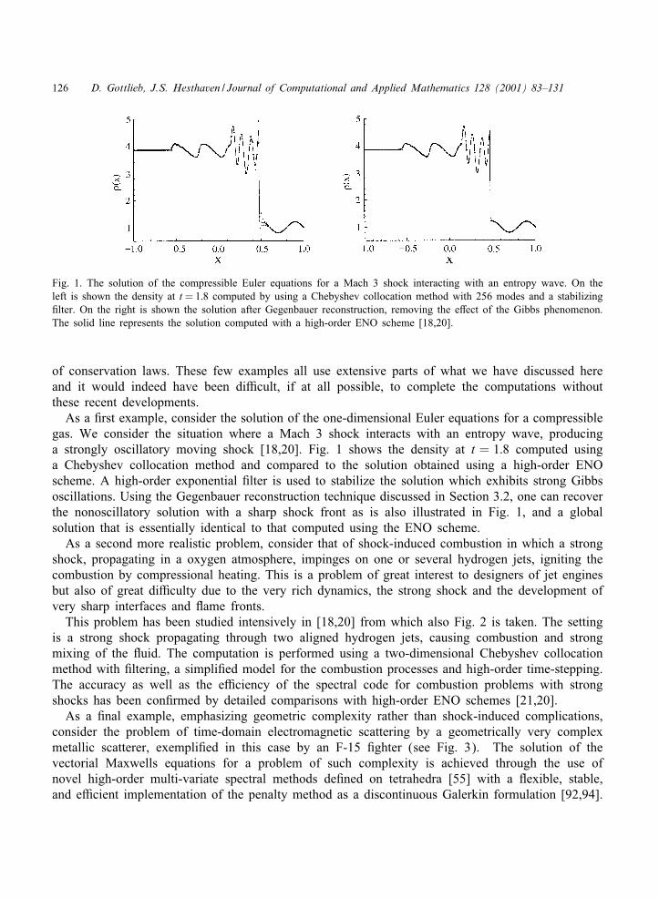
126 D. Gottlieb, J.S. Hesthaven / Journal of Computational and Applied Mathematics 128 (2001) 83–131
Fig. 1. The solution of the compressible Euler equations for a Mach 3 shock interacting with an entropy wave. On theleft is shown the density at t = 1:8 computed by using a Chebyshev collocation method with 256 modes and a stabilizing1lter. On the right is shown the solution after Gegenbauer reconstruction, removing the e8ect of the Gibbs phenomenon.The solid line represents the solution computed with a high-order ENO scheme [18,20].
of conservation laws. These few examples all use extensive parts of what we have discussed hereand it would indeed have been di9cult, if at all possible, to complete the computations withoutthese recent developments.
As a 1rst example, consider the solution of the one-dimensional Euler equations for a compressiblegas. We consider the situation where a Mach 3 shock interacts with an entropy wave, producinga strongly oscillatory moving shock [18,20]. Fig. 1 shows the density at t = 1:8 computed usinga Chebyshev collocation method and compared to the solution obtained using a high-order ENOscheme. A high-order exponential 1lter is used to stabilize the solution which exhibits strong Gibbsoscillations. Using the Gegenbauer reconstruction technique discussed in Section 3.2, one can recoverthe nonoscillatory solution with a sharp shock front as is also illustrated in Fig. 1, and a globalsolution that is essentially identical to that computed using the ENO scheme.
As a second more realistic problem, consider that of shock-induced combustion in which a strongshock, propagating in a oxygen atmosphere, impinges on one or several hydrogen jets, igniting thecombustion by compressional heating. This is a problem of great interest to designers of jet enginesbut also of great di9culty due to the very rich dynamics, the strong shock and the development ofvery sharp interfaces and Iame fronts.
This problem has been studied intensively in [18,20] from which also Fig. 2 is taken. The settingis a strong shock propagating through two aligned hydrogen jets, causing combustion and strongmixing of the Iuid. The computation is performed using a two-dimensional Chebyshev collocationmethod with 1ltering, a simpli1ed model for the combustion processes and high-order time-stepping.The accuracy as well as the e9ciency of the spectral code for combustion problems with strongshocks has been con1rmed by detailed comparisons with high-order ENO schemes [21,20].
As a 1nal example, emphasizing geometric complexity rather than shock-induced complications,consider the problem of time-domain electromagnetic scattering by a geometrically very complexmetallic scatterer, exempli1ed in this case by an F-15 1ghter (see Fig. 3). The solution of thevectorial Maxwells equations for a problem of such complexity is achieved through the use ofnovel high-order multi-variate spectral methods de1ned on tetrahedra [55] with a Iexible, stable,and e9cient implementation of the penalty method as a discontinuous Galerkin formulation [92,94].
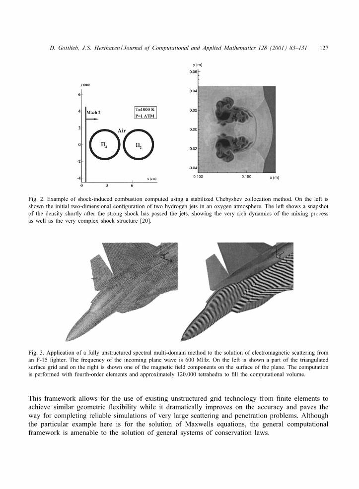
D. Gottlieb, J.S. Hesthaven / Journal of Computational and Applied Mathematics 128 (2001) 83–131 127
Fig. 2. Example of shock-induced combustion computed using a stabilized Chebyshev collocation method. On the left isshown the initial two-dimensional con1guration of two hydrogen jets in an oxygen atmosphere. The left shows a snapshotof the density shortly after the strong shock has passed the jets, showing the very rich dynamics of the mixing processas well as the very complex shock structure [20].
Fig. 3. Application of a fully unstructured spectral multi-domain method to the solution of electromagnetic scattering froman F-15 1ghter. The frequency of the incoming plane wave is 600 MHz. On the left is shown a part of the triangulatedsurface grid and on the right is shown one of the magnetic 1eld components on the surface of the plane. The computationis performed with fourth-order elements and approximately 120.000 tetrahedra to 1ll the computational volume.
This framework allows for the use of existing unstructured grid technology from 1nite elements toachieve similar geometric Iexibility while it dramatically improves on the accuracy and paves theway for completing reliable simulations of very large scattering and penetration problems. Althoughthe particular example here is for the solution of Maxwells equations, the general computationalframework is amenable to the solution of general systems of conservation laws.

128 D. Gottlieb, J.S. Hesthaven / Journal of Computational and Applied Mathematics 128 (2001) 83–131
While the developments of spectral methods during the last decade have been very signi1cant,a number of critical issues remains open. On the theoretical side, many issues related to stability,even for linear problems, remains open. The results are naturally even more sparse for nonlinearproblems. In many instances the experienced user of spectral methods can do much more than canbe justi1ed — and often with remarkable success.
Spectral collocation methods have reached a level of sophistication and maturity where it allowsfor the accurate and e9cient solution of nonlinear problems with strong discontinuities using only onedomain. For smooth problems, one the other hand, the development of multi-domain formulations hasreached a level where it allows for the e9cient and accurate solution of problems of almost arbitrarygeometric complexity. One of the great challenges of the immediate future lies in understandinghow to do strongly nonlinear conservation laws in complex geometries in a stable manner using aspectrally accurate, geometrically Iexible, and computationally e9cient formulation.
References
[1] S. Abarbanel, D. Gottlieb, E. Tadmor, Spectral methods for discontinuous problems, in: K.W. Morton, M.J. Baines(Eds.), Numerical methods for Iuid dynamics II, Clarendon Press, Oxford, 1986, pp. 129–153.
[2] I. Andreassen, I. Lie, Simulation of acoustical and elastic waves and interaction, J. Acoust. Soc. Am. 95 (1994)171–186.
[3] N.S. Banerjee, J. Geer, Exponential approximations using fourier series partial sums, ICASE Report No. 97-56,NASA Langley Research Center, VA, 1997.
[4] G. Ben-Yu, Spectral Methods and Their Applications, World Scienti1c, Singapore, 1998.[5] C. Bernardi, Y. Maday, Polynomial interpolation results in sobolev spaces, J. Comput. Appl. Math. 43 (1992) 53–80.[6] C. Bernardi, Y. Maday, Spectral methods, in: P.G. Ciarlet, J.L. Lions (Eds.), Handbook of Numerical Analysis V,
Elsevier Sciences, North-Holland, The Netherlands, 1999.[7] J.P. Boyd, Two comments on 1ltering (arti1cial viscosity) for Chebyshev and Legendre spectral and spectral element
methods: preserving boundary conditions and interpretation of the 1lter as a di8usion, J. Comput. Phys. 143 (1998)283–288.
[8] W. Cai, D. Gottlieb, C.W. Shu, Essentially nonoscillatory spectral fourier methods for shock wave calculations,Math. Comp. 52 (1989) 389–410.
[9] W. Cai, D. Gottlieb, A. Harten, Cell averaging Chebyshev methods for hyperbolic problems, in: Computers andMathematics with Applications, Academic Press, New York, 1990.
[10] C. Canuto, M.Y. Hussaini, A. Quarteroni, T.A. Zang, Spectral Methods in Fluid Dynamics, Springer Series inComputational Physics, Springer, New York, 1988.
[11] C. Canuto, A. Quarteroni, Error estimates for spectral and pseudospectral approximations of hyperbolic equations,SIAM J. Numer. Anal. 19 (1982) 629–642.
[12] C. Canuto, A. Quarteroni, Approximation results for orthogonal polynomials in sobolev spaces, Math. Comput. 38(1982) 67–86.
[13] M.H. Carpenter, D. Gottlieb, Spectral methods on arbitrary grids, J. Comput. Phys. 129 (1996) 74–86.[14] M.H. Carpenter, D. Gottlieb, C.W, Shu, On the Law-Wendro8 theorem for spectral methods, (2000), in preparation.[15] G.Q. Chen, Q. Du, E. Tadmor, Spectral viscosity approximations to multidimensional scalar conservation laws, Math.
Comp. 61 (1993) 629–643.[16] B. Cockburn, C.W. Shu, Discontinuous Galerkin methods for convection-dominated problems, SIAM Rev. (2000),
submitted for publication.[17] L. Dettori, B. Yang, On the Chebyshev penalty method for parabolic and hyperbolic equations, M2AN 30 (1996)
907–920.[18] W.S. Don, Numerical study of pseudospectral methods in shock wave applications, J. Comput. Phys. 110 (1994)
103–111.
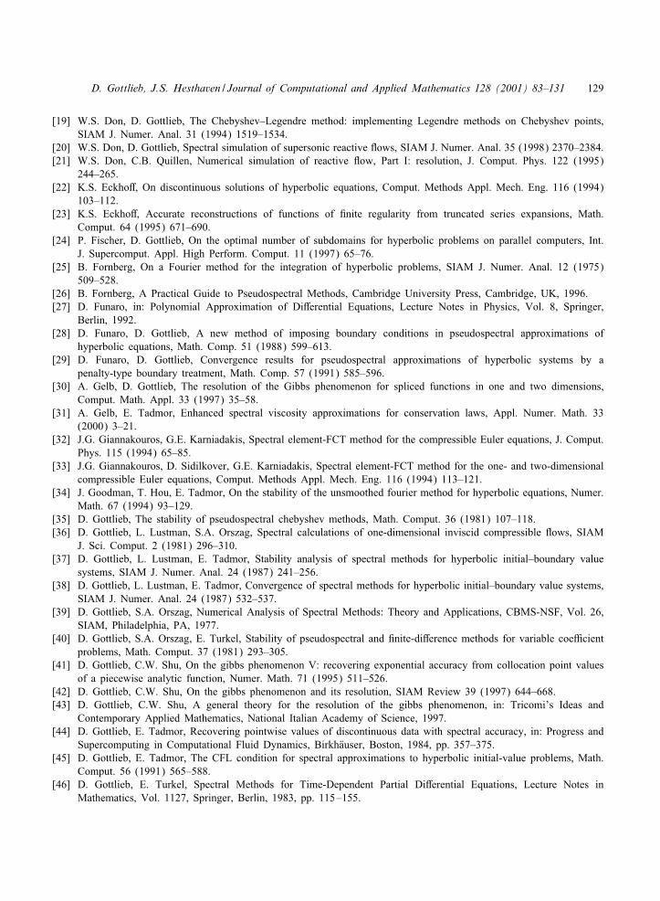
D. Gottlieb, J.S. Hesthaven / Journal of Computational and Applied Mathematics 128 (2001) 83–131 129
[19] W.S. Don, D. Gottlieb, The Chebyshev–Legendre method: implementing Legendre methods on Chebyshev points,SIAM J. Numer. Anal. 31 (1994) 1519–1534.
[20] W.S. Don, D. Gottlieb, Spectral simulation of supersonic reactive Iows, SIAM J. Numer. Anal. 35 (1998) 2370–2384.[21] W.S. Don, C.B. Quillen, Numerical simulation of reactive Iow, Part I: resolution, J. Comput. Phys. 122 (1995)
244–265.[22] K.S. Eckho8, On discontinuous solutions of hyperbolic equations, Comput. Methods Appl. Mech. Eng. 116 (1994)
103–112.[23] K.S. Eckho8, Accurate reconstructions of functions of 1nite regularity from truncated series expansions, Math.
Comput. 64 (1995) 671–690.[24] P. Fischer, D. Gottlieb, On the optimal number of subdomains for hyperbolic problems on parallel computers, Int.
J. Supercomput. Appl. High Perform. Comput. 11 (1997) 65–76.[25] B. Fornberg, On a Fourier method for the integration of hyperbolic problems, SIAM J. Numer. Anal. 12 (1975)
509–528.[26] B. Fornberg, A Practical Guide to Pseudospectral Methods, Cambridge University Press, Cambridge, UK, 1996.[27] D. Funaro, in: Polynomial Approximation of Di8erential Equations, Lecture Notes in Physics, Vol. 8, Springer,
Berlin, 1992.[28] D. Funaro, D. Gottlieb, A new method of imposing boundary conditions in pseudospectral approximations of
hyperbolic equations, Math. Comp. 51 (1988) 599–613.[29] D. Funaro, D. Gottlieb, Convergence results for pseudospectral approximations of hyperbolic systems by a
penalty-type boundary treatment, Math. Comp. 57 (1991) 585–596.[30] A. Gelb, D. Gottlieb, The resolution of the Gibbs phenomenon for spliced functions in one and two dimensions,
Comput. Math. Appl. 33 (1997) 35–58.[31] A. Gelb, E. Tadmor, Enhanced spectral viscosity approximations for conservation laws, Appl. Numer. Math. 33
(2000) 3–21.[32] J.G. Giannakouros, G.E. Karniadakis, Spectral element-FCT method for the compressible Euler equations, J. Comput.
Phys. 115 (1994) 65–85.[33] J.G. Giannakouros, D. Sidilkover, G.E. Karniadakis, Spectral element-FCT method for the one- and two-dimensional
compressible Euler equations, Comput. Methods Appl. Mech. Eng. 116 (1994) 113–121.[34] J. Goodman, T. Hou, E. Tadmor, On the stability of the unsmoothed fourier method for hyperbolic equations, Numer.
Math. 67 (1994) 93–129.[35] D. Gottlieb, The stability of pseudospectral chebyshev methods, Math. Comput. 36 (1981) 107–118.[36] D. Gottlieb, L. Lustman, S.A. Orszag, Spectral calculations of one-dimensional inviscid compressible Iows, SIAM
J. Sci. Comput. 2 (1981) 296–310.[37] D. Gottlieb, L. Lustman, E. Tadmor, Stability analysis of spectral methods for hyperbolic initial–boundary value
systems, SIAM J. Numer. Anal. 24 (1987) 241–256.[38] D. Gottlieb, L. Lustman, E. Tadmor, Convergence of spectral methods for hyperbolic initial–boundary value systems,
SIAM J. Numer. Anal. 24 (1987) 532–537.[39] D. Gottlieb, S.A. Orszag, Numerical Analysis of Spectral Methods: Theory and Applications, CBMS-NSF, Vol. 26,
SIAM, Philadelphia, PA, 1977.[40] D. Gottlieb, S.A. Orszag, E. Turkel, Stability of pseudospectral and 1nite-di8erence methods for variable coe9cient
problems, Math. Comput. 37 (1981) 293–305.[41] D. Gottlieb, C.W. Shu, On the gibbs phenomenon V: recovering exponential accuracy from collocation point values
of a piecewise analytic function, Numer. Math. 71 (1995) 511–526.[42] D. Gottlieb, C.W. Shu, On the gibbs phenomenon and its resolution, SIAM Review 39 (1997) 644–668.[43] D. Gottlieb, C.W. Shu, A general theory for the resolution of the gibbs phenomenon, in: Tricomi’s Ideas and
Contemporary Applied Mathematics, National Italian Academy of Science, 1997.[44] D. Gottlieb, E. Tadmor, Recovering pointwise values of discontinuous data with spectral accuracy, in: Progress and
Supercomputing in Computational Fluid Dynamics, BirkhYauser, Boston, 1984, pp. 357–375.[45] D. Gottlieb, E. Tadmor, The CFL condition for spectral approximations to hyperbolic initial-value problems, Math.
Comput. 56 (1991) 565–588.[46] D. Gottlieb, E. Turkel, Spectral Methods for Time-Dependent Partial Di8erential Equations, Lecture Notes in
Mathematics, Vol. 1127, Springer, Berlin, 1983, pp. 115–155.
130 D. Gottlieb, J.S. Hesthaven / Journal of Computational and Applied Mathematics 128 (2001) 83–131
[47] D. Gottlieb, C.E. Wasberg, Optimal strategy in domain decomposition spectral methods for wave-like phenomena,SIAM J. Sci. Comput. (1999), to appear.
[48] J.S. Hesthaven, A stable penalty method for the compressible Navier–Stokes equations: II, one-dimensional domaindecomposition schemes, SIAM J. Sci. Comput. 18 (1997) 658–685.
[49] J.S. Hesthaven, A stable penalty method for the compressible Navier–stokes equations: III, multidimensional domaindecomposition schemes, SIAM J. Sci. Comput. 20 (1999) 62–93.
[50] J.S. Hesthaven, Spectral penalty methods, Appl. Numer. Math. 33 (2000) 23–41.[51] J.S. Hesthaven, P.G. Dinesen, J.P. Lynov, Spectral collocation time-domain modeling of di8ractive optical elements,
J. Comput. Phys. 155 (1999) 287–306.[52] J.S. Hesthaven, D. Gottlieb, A stable penalty method for the compressible Navier–Stokes equations, I, open boundary
conditions, SIAM J. Sci. Comput. 17 (1996) 579–612.[53] J.S. Hesthaven, D. Gottlieb, Stable spectral methods for conservation laws on triangles with unstructured grids,
Comput. Methods Appl. Mech. Eng. 175 (1999) 361–381.[54] J.S. Hesthaven, J. Juul Rasmussen, L. BergZe, J. Wyller, Numerical studies of localized wave 1elds govenered by the
Raman-extended derivative nonlinear SchrYodinger equation, J. Phys. A: Math. Gen. 30 (1997) 8207–8224.[55] J.S. Hesthaven, C.H. Teng, Stable spectral methods on tetrahedral elements, SIAM J. Sci. Comput. (2000), to appear.[56] E. Isaacson, H.B. Keller, Analysis of Numerical Methods, Dover Publishing, New York, 1966.[57] D. Jackson, The Theory of Approximation, American Mathematical Society, Colloquim Publication, Vol. 11,
Providence, RI, 1930.[58] D.A. Kopriva, A spectral multidomain method for the solution of hyperbolic systems, Appl. Numer. Math. 2 (1986)
221–241.[59] D.A. Kopriva, Computation of hyperbolic equations on complicated domains with patched and overset chebyshev
grids, SIAM J. Sci. Statist. Comput. 10 (1989) 120–132.[60] D.A. Kopriva, Multidomain spectral solution of the Euler gas-dynamics equations, J. Comput. Phys. 96 (1991)
428–450.[61] D.A. Kopriva, A conservative staggered-grid Chebyshev multidomain method for compressible Iows, II, a
semi-structured method, J. Comput. Phys. 128 (1996) 475–488.[62] D.A. Kopriva, J.H. Kolias, A conservative staggered-grid Chebyshev multidomain method for compressible Iows,
II, a semi-structured method, J. Comput. Phys. 125 (1996) 244–261.[63] D.A. Kopriva, S.L. Woodru8, M.Y. Hussaini, Discontinuous spectral element approximation of Maxwell’s equations,
in: B. Cockburn, G.E. Karniadakis, C.W. Shu (Eds.), Discontinuous Galerkin Methods: Theory, Computation andApplications, Lecture Notes in Computational Science and Engineering, Vol. 11, Springer, New York, 2000, pp.355–362.
[64] H.O. Kreiss, J. Lorenz, Initial-Boundary Value Problems and the Navier–Stokes Equations, Series in Pure and AppliedMathematics, Academic Press, San Diego, 1989.
[65] H.O. Kreiss, J. Oliger, Comparison of accurate methods for the integration of hyperbolic problems, Tellus 24 (1972)199–215.
[66] H.O. Kreiss, J. Oliger, Stability of the Fourier method, SIAM J. Numer. Anal. 16 (1979) 421–433.[67] P.D. Lax (Ed.), Accuracy and resolution in the computation of solutions of linear and nonlinear equations, in:
Proceedings of Recent Advances in Numerical Analysis, University of Wisconsin, Academic Press, New York,1978, pp. 107–117.
[68] D. Levy, E. Tadmor, From semi-discrete to fully-discrete: stability of Runge–Kutta schemes by the energy method,SIAM Rev. 40 (1998) 40–73.
[69] I. Lomtev, C.B. Quillen, G.E. Karniadakis, Spectral=hp methods for viscous compressible Iows on unstructured 2Dmeshes, J. Comput. Phys. 144 (1998) 325–357.
[70] H. Ma, Chebyshev–Legendre super spectral viscosity method for nonlinear conservation laws, SIAM J. Numer. Anal.35 (1998) 869–892.
[71] H. Ma, Chebyshev–Legendre spectral viscosity method for nonlinear conservation laws, SIAM J. Numer. Anal. 35(1998) 893–908.
[72] Y. Maday, E. Tadmor, Analysis of the spectral vanishing viscosity method for periodic conservation laws, SIAM J.Numer. Anal. 26 (1989) 854–870.

D. Gottlieb, J.S. Hesthaven / Journal of Computational and Applied Mathematics 128 (2001) 83–131 131
[73] Y. Maday, S.M. Ould Kaper, E. Tadmor, Legendre pseudospectral viscosity method for nonlinear conservation laws,SIAM J. Numer. Anal. 30 (1993) 321–342.
[74] A. Majda, J. McDonough, S. Osher, The Fourier method for nonsmooth initial data, Math. Comp. 32 (1978) 1041–1081.
[75] S.A. Orszag, Comparison of pseudospectral and spectral approximation, Stud. Appl. Math. 51 (1972) 253–259.[76] J.E. Pasciak, Spectral and pseudospectral methods for advection equations, Math. Comp. 35 (1980) 1081–1092.[77] A. Quarteroni, Domain decomposition methods for systems of conservation laws: spectral collocation approximations,
SIAM J. Sci. Statist. Comput. 11 (1990) 1029–1052.[78] S.C. Reddy, L.N. Trefethen, Lax-stability of fully discrete spectral methods via stability regions and
pseudo-eigenvalues, Comput. Methods Appl. Mech. Eng. 80 (1990) 147–164.[79] S.C. Reddy, L.N. Trefethen, Stability of the method of lines, Numer. Math. 62 (1992) 235–267.[80] D. Sidilkover, G.E. Karniadakis, Non-oscillatory spectral element Chebyshev method for shock wave calculations, J.
Comput. Phys. 107 (1993) 10–22.[81] G. Szego, in: Orthogonal polynomials, 4th Edition, American Mathematical Society, Vol. 23, Colloquim Publication,
Providence, RI, 1975.[82] E. Tadmor, Skew-selfadjoint form for systems of conservation laws, J. Math. Anal. Appl. 103 (1984) 428–442.[83] E. Tadmor, The exponential accuracy of fourier and Chebyshev di8erencing methods, SIAM Rev. 23 (1986) 1–10.[84] E. Tadmor, Stability analysis of 1nite-di8erence, pseudospectral, and Fourier–Galerkin approximations for
time-dependent problems, SIAM Rev. 29 (1987) 525–555.[85] E. Tadmor, Convergence of spectral methods for nonlinear conservation laws, SIAM J. Numer. Anal. 26 (1989)
30–44.[86] H. Tal-Ezer, Ph.D. Thesis, Tel Aviv University, 1983.[87] L.N. Trefethen, M.R. Trummer, An instability phenomenon in spectral methods, SIAM J. Numer. Anal. 24 (1987)
1008–1023.[88] H. Vandeven, Family of spectral 1lters for discontinuous problems, J. Sci. Comput. 8 (1991) 159–192.[89] L. Vozovoi, M. Israeli, A. Averbuch, Analysis and application of Fourier–Gegenbauer method to sti8 di8erential
equations, SIAM J. Numer. Anal. 33 (1996) 1844–1863.[90] L. Vozovoi, A. Weill, M. Israeli, Spectrally accurate solution of nonperiodic di8erential equations by the Fourier–
Gegenbauer method, SIAM J. Numer. Anal. 34 (1997) 1451–1471.[91] T. Warburton, G.E. Karniadakis, A discontinuous Galerkin method for the viscous MHD equations, J. Comput. Phys.
152 (1999) 608–641.[92] T. Warburton, Application of the discontinuous Galerkin method to Maxwell’s equations using unstructured
polymorphic hp-1nite elements, in: B. Cockburn, G.E. Karniadakis, C.W. Shu (Eds.), Discontinuous GalerkinMethods: Theory, Computation and Applications. Lecture Notes in Computational Science and Engineering, Vol.11, Springer, New York, 2000, pp. 451–458.
[93] T. Warburton, I. Lomtev, Y. Du, S. Sherwin, G.E. Karniadakis, Galerkin and discontinuous Galerkin spectral=hpmethods, Comput. Methods Appl. Mech. Eng. 175 (1999) 343–359.
[94] T. Warburton, J.S. Hesthaven, Stable unstructured grid scheme for Maxwells equations, J. Comput. Phys. (2000),submitted for publication.
[95] B. Yang, D. Gottlieb, J.S. Hesthaven, Spectral simulations of electromagnetic wave scattering, J. Comput. Phys. 134(1997) 216–230.
[96] B. Yang, J.S. Hesthaven, A pseudospectral method for time-domain computation of electromagnetic scattering bybodies of revolution, IEEE Trans. Antennas and Propagation 47 (1999) 132–141.
[97] B. Yang, J.S. Hesthaven, Multidomain pseudospectral computation of Maxwells equations in 3-D general curvilinearcoordinates, Appl. Numer. Math. 33 (2000) 281–289.

Journal of Computational and Applied Mathematics 128 (2001) 133–185www.elsevier.nl/locate/cam
Wavelet methods for PDEs — some recent developmentsWolfgang Dahmen1
Institut f�ur Geometrie und Praktische Mathematik, RWTH Aachen, Templergraben 55, 52056 Aachen,Germany
Received 5 July 1999; received in revised form 7 December 1999
Abstract
This paper is concerned with recent developments of wavelet schemes for the numerical treatment of operator equationswith special emphasis on two issues: adaptive solution concepts and nontrivial domain geometries. After describing ageneral multiresolution framework the key features of wavelet bases are highlighted, namely locality, norm equivalencesand cancellation properties. Assuming 3rst that wavelet bases with these properties are available on the relevant problemdomains, the relevance of these features for a wide class of stationary problems is explained in subsequent sections. Themain issues are preconditioning and the e5cient (adaptive) application of wavelet representations of the involved operators.We indicate then how these ingredients combined with concepts from nonlinear or best N -term approximation culminatein an adaptive wavelet scheme for elliptic selfadjoint problems covering boundary value problems as well as boundaryintegral equations. These schemes can be shown to exhibit convergence rates that are in a certain sense asymptoticallyoptimal. We conclude this section with some brief remarks on data structures and implementation, interrelations withregularity in a certain scale of Besov spaces and strategies of extending such schemes to unsymmetric or inde3niteproblems. We address then the adaptive evaluation of nonlinear functionals of wavelet expansions as a central taskarising in connection with nonlinear problems. Wavelet bases on nontrivial domains are discussed next. The main issuesare the development of Fourier free construction principles and criteria for the validity of norm equivalences. Finally,we indicate possible combinations of wavelet concepts with conventional discretizations such as 3nite element or 3nitevolume schemes in connection with convection dominated and hyperbolic problems. c© 2001 Elsevier Science B.V. Allrights reserved.
MSC: 41A25; 41A46; 46A35; 46B03; 65F35; 65N12; 65N55; 65R20; 65Y20
Keywords: Multiresolution; Wavelet bases; Norm equivalences; Cancellation properties; Preconditioning; Multiscaletransformations; Best N -term approximation; Fast matrix/vector multiplication; Adaptive solvers; Convergence rates;Besov regularity; Nonlinear functionals of wavelet expansions; Wavelet bases on domains; Fourier free criteria; Stablecompletions; Direct and inverse estimates; Domain decomposition; Convection dominated problems; Hyperbolic problems
1 WWW: http:==www.igpm.rwth-aachen.de=∼dahmen=E-mail address: [email protected] (W. Dahmen).
0377-0427/01/$ - see front matter c© 2001 Elsevier Science B.V. All rights reserved.PII: S 0377-0427(00)00511-2
134 W. Dahmen / Journal of Computational and Applied Mathematics 128 (2001) 133–185
1. Introduction
Quoting from [67] the concept of wavelets can be viewed as a synthesis of ideas which originatedduring the last 30 years from engineering (subband coding), physics (coherent states, renormaliza-tion group) and pure mathematics (CalderHon–Zygmund operators). In addition the construction ofspline bases for Banach spaces can be viewed as a further relevant source from pure mathematics[30]. It is understandable that this multitude of origins appeal to scientists in many diJerent areas.Consequently, the current research landscape concerned with wavelet ideas is extremely varied. Hereis an incomplete list of related active topics: construction of wavelets; wavelets as tools in interdis-ciplinary applications; wavelets as modeling tools; wavelets as analysis tools; multiscale geometryrepresentation; wavelets in statistics; wavelets in numerical analysis and large-scale computation.The main focus of this article will be on recent developments in the last area. Rather than trying to
give an exhaustive account of the state of the art I would like to bring out some mechanisms whichare in my opinion important for the application of wavelets to operator equations. To accomplish thisI found it necessary to address some of the pivotal issues in more detail than others. Nevertheless,such a selected ‘zoom in’ supported by an extensive list of references should provide a sound footingfor conveying also a good idea about many other related branches that will only be brieMy touchedupon. Of course, the selection of material is biased by my personal experience and therefore is notmeant to reMect any objective measure of importance. The paper is organized around two essentialissues namely adaptivity and the development of concepts for coping with a major obstruction inthis context namely practically relevant domain geometries.
Being able to solve a given large scale discrete problem in optimal time is one important step.In this regard a major breakthrough has been caused by multi-grid methods. A further, sometimesperhaps even more dramatic reduction of complexity may result from adapting in addition thediscretization to the individual application at hand. This means to realize a desired overall accuracyat the expense of a possibly small number of involved degrees of freedom.
A central theme in subsequent discussions is to indicate why wavelet concepts appear to beparticularly promising in this regard. In fact, the common attraction of wavelets in all the above listedareas hinges on their principal ability of organizing the decomposition of an object into componentscharacterized by diJerent length scales. This calls for locally adapting the level of resolution and haslong been praised as a promising perspective. As intuitive as this might be a quantitative realizationof such ideas faces severe obstructions. This note is to reMect some of the ideas that have beendriving these developments. A more detailed account of a much wider scope of related topics canbe found in [31,49].
The material is organized as follows. After collecting some preliminaries in Section 2, Section 3is devoted to a discussion of two central features which are fundamental for wavelet concepts innumerical analysis namely cancellation properties and isomorphisms between function and sequencespaces. Assuming at this point that wavelet bases with these properties are indeed available (evenfor nontrivial domains) some consequences of these features are described in subsequent sections.Section 4 addresses preconditioning for elliptic problems as well as the connection with nonlinearor best N -term approximation. Section 5 is concerned with the e7ciency of matrix=vector multi-plications when working in wavelet coordinates. In particular, some implications pertaining to thetreatment of boundary integral equations are outlined. It is indicated in Section 6 how these conceptsenter the analysis of an adaptive scheme for a wide class of elliptic operator equations. Since these
W. Dahmen / Journal of Computational and Applied Mathematics 128 (2001) 133–185 135
rather recent results reMect in my opinion the potential of wavelet methodologies quite well andsince the involved tools are probably not very familiar in the numerical analysis community a some-what more detailed discussion of this topic is perhaps instructive. In Section 7 a basic ingredientfor the treatment of nonlinear problems is discussed namely the adaptive computation of nonlin-ear functionals of multiscale expansions. In particular, a recent fast evaluation scheme is sketched.Section 8 is concerned with the practical realization of those properties of wavelet bases that havebeen identi3ed before as being crucial. This covers “Fourier free” criteria for norm equivalences aswell as several construction principles such as stable completions or the lifting scheme. It is thenindicated in Section 9 how to use these concepts for the concrete construction of wavelet bases onbounded domains. In particular, this covers an approach that leads in a natural way to convergentdomain decomposition schemes for singular integral equations. Some remarks on 3nite element basedwavelet bases conclude this section. Finally, we brieMy touch in Section 10 upon recent applicationsof adaptive wavelet concepts within conventional 3nite element or 3nite volume discretization forconvection diJusion equations, respectively hyperbolic conservation laws.
For convenience we will write a. b to express that a can be bounded by some constant multipleof b uniformly in all parameters on which a and b might depend as long as the precise value ofsuch constants does not matter. Likewise a∼ b means a. b and b. a.
2. Some preliminary comments
2.1. About the general spirit
To motivate the subsequent discussions consider an admittedly oversimpli3ed example namelythe representation of a real number x by means of decimal or more generally p-adic expansionsx=
∑−∞j=l djbj; where b is the base, b=10, say. An irrational number is an array of in8nitely many
digits. Depending on the context such a number may only be needed up to a certain accuracy sayinghow many digits are required. So in a sense one may identify the number with an algorithm thatproduces the required number of digits. It is therefore natural to ask: Is there anything similar forfunctions? Of course, all classical expansions of Laurent, Taylor or Fourier type reMect exactly thispoint of view. WeierstraT was only willing to call an object a function if it could be in principlecomputed through a countable number of basic arithmetic operations based on such an expansion.A wavelet basis �={ I : I ∈J} (where J is a suitable index set to be commented on later in moredetail) is in this sense just another collection of basis functions in terms of which a given functionf can be expanded
f =∑I ∈J
dI (f) I : (2.1)
Such an expansion associates with f the array d = {dI (f)}I ∈J of digits. There are a few pointsthough by which a wavelet expansion diJers from more classical expansions. First of all, for instance,a Taylor expansion puts strong demands on the regularity of f such as analyticity, while (2.1) istypically valid for much larger classes of functions such as square integrable ones. By this we meanthat the series on the right-hand side of (2.1) converges in the corresponding norm. More importantly,the digits dI convey very detailed information on f. To explain this, a word on the indices I ∈J
136 W. Dahmen / Journal of Computational and Applied Mathematics 128 (2001) 133–185
is in order. Each I comprises information of diJerent type such as scale and spatial location. Forinstance, classical wavelets on the real line are generated by scaling and translating a single function , i.e., j; k =2j=2 (2j · −k). The simplest example is to take the box function � := �[0;1) to form theHaar wavelet := (�(2·) − �(2 · −1))=√2. Obviously is orthogonal to �. It is easy to see thatthe collection of functions {�(· − k): k ∈Z} ∪ {2j=2 (2j · −k): k; j∈Z} forms an orthonormal basisfor L2(R). Likewise {�} ∪ {2j=2 (2j · −k): k = 0; : : : ; 2j − 1; j = 0; 1; : : :} is an orthonormal basis ofL2([0; 1]). In this case one has (j; k)↔ I . Note that the whole basis consists in both examples of twogroups of functions namely the box functions on a 3xed coarsest level and the set of ‘true’ waveletson all successively higher levels. When expanding a function in such a basis the box functions areneeded to recover the constant part while the rest encodes further updates. Such a coarsest level isusually needed when dealing with bounded domains. When employing isotropic scaling by powersof two, wavelets on Rd are obtained by scaling and translating 2d−1 3xed functions 2jd=2 e(2j ·−k),e∈{0; 1}d\{0} so that then I ↔ (j; k; e). For more general domains one has to relax the strictinterrelation through translation but the nature of the indices will stay essentially the same as will beexplained later for corresponding examples. At this point it su5ces to denote by j = |I | the scale jand by k the location k of the wavelet I . This means that I is associated with detail informationof length scale 2−|I | around a spatial location encoded by k. In particular, when the wavelets havecompact support the diameter of the support of a wavelet on level |I | behaves like
diam supp I ∼ 2−|I |: (2.2)
Thus when the coe5cient |dI (f)| is large this indicates that near k(I) the function f has signi3cantcomponents of length scale 2−|I |.
Another characteristic feature of wavelets is that certain weighted sequence norms of the coe5-cients in a wavelet expansion are equivalent to certain function space norms of the correspondingfunctions. Again the Haar basis serves as the simplest example where the function space is L2 andthe Euclidean norm is used to measure the coe5cients. This implies, in particular, that discardingsmall wavelet coe5cients, results in small perturbations of the function in that norm. In a 3nite dif-ference or 3nite element context adaptivity is typically associated with local mesh re8nement wherethe re3nement criteria are extracted from foregoing calculations usually with the aid of a posteriorierror bounds or indicators. In the case of wavelet analysis the concept is somewhat diJerent. Incontrast to approximating the solution of a given operator equation on some mesh (of 3xed highestresolution) wavelet-based schemes aim at determining its representation with respect to a basis. Thisseems to be a minor distinction of primarily philosophical nature but turns out to suggest a ratherdiJerent way of thinking. In fact, adaptivity then means to track during the solution process onlythose coe5cients in the unknown array d(f) in (2.1) that are most signi8cant for approximating fwith possibly few degrees of freedom.
2.2. Fourier techniques
Part of the fascination about wavelets stems from the fact that a conceptually fairly simple math-ematical object oJers at least an extremely promising potential in several important applicationareas. The technical simplicity and the practicality of this object, however, is by no means inde-pendent of its domain of de3nition. The development of wavelets has been largely inMuenced byFourier techniques and harmonic analysis concepts, quite in agreement with the nature of the primary
W. Dahmen / Journal of Computational and Applied Mathematics 128 (2001) 133–185 137
application areas. Fourier techniques not only account for the elegance of constructions but also forthe analysis of applications [34,67]. It is therefore quite natural that 3rst attempts of expanding theapplication of wavelet techniques to other areas such as numerical analysis tried to exploit the ad-vantages of Fourier concepts. To a get a quick impression of the potential suggests to consider 3rstmodel problems that help minimizing severe technical obstructions. Consequently periodic problemshave largely served as test beds for such investigations. As much as one might argue about thepracticability of such settings these investigations have been of pioneering importance. For instance,Beylkin et al. [15] has initiated important developments centering on matrix compression and fastprocessing of certain densely populated matrices. Likewise the concept of vaguelette draws on ideasfrom the theory of CalderHon–Zygmund operators [87,110]. Putting more weight on the actual inver-sion of operators complements traditional thinking in numerical analysis, see e.g. [5,16,87,92,49] fora more detailed exposition and further references. Among other things these developments have ledto interesting applications, for instance, in physical modeling concerning the simulation of coherentstates in 2D turbulent Mows or combustion [8,18,102]. Again for details the reader is referred to theoriginal literature.
2.3. The curse of geometry
Nevertheless, the periodic setting poses severe limitations because it excludes, for instance, do-main induced singularities or turbulent behavior due to no slip boundary conditions. However, anumber of obstructions arise when leaving the periodic realm. First of all the essential features ofwavelets closely tied to Fourier concepts have to be re-identi3ed in a correspondingly more Mexiblecontext. New construction principles are needed. Thus, the systematic development of conceptualsubstitutes for Fourier techniques is of pivotal importance and will be a recurrent theme in subse-quent discussions, see e.g. [26,46,48,49,108,109] for contributions in this spirit. We will outline nexta multi-resolution framework which is Mexible enough to cover later applications of varying nature.
2.4. Multi-resolution
Recall that a convenient framework for constructing and analyzing wavelets on Rd is the conceptof multi-resolution approximation formalized in [93]. Here is a somewhat generalized variant ofmulti-resolution that will work later for more general domain geometries. To this end, consider anascending sequence S of closed nested spaces Sj; j∈N0, Sj⊂ Sj+1 whose union is dense in a givenBanach space B, say. A particularly important case arises when B=H is a Hilbert space with innerproduct 〈·; ·〉 and norm ‖ · ‖H := 〈·; ·〉1=2. In the classical multi-resolution setting as well as in allcases of practical interest the spaces Sj are spanned by what will be called a single-scale basis�j = {�j;k : k ∈Ij}, i.e., Sj = span�j =: S (�j). In view of the intended applications, we considerhere only 3nite-dimensional spaces Sj. Moreover, we are only interested in local bases, i.e., as in(2.2)
diam supp�j;k ∼ 2−j: (2.3)
Nestedness of the Sj implies then that the �j;k satisfy a two-scale or re8nement relation
�j;k =∑
l∈Ij+1
mj;l; k�j+1; l; k ∈Ij: (2.4)

138 W. Dahmen / Journal of Computational and Applied Mathematics 128 (2001) 133–185
Collecting the 8lter or mask coe7cients mj;l; k in the Ij+1 × Ij-matrix Mj;0 = (mj;l; k)l∈Ij+1 ; k ∈Ij ,(2.4) is conveniently expresses as a matrix=vector relation
�Tj = �T
j+1Mj;0: (2.5)
The simplest example has been described above when H = L2([0; 1]) and the Sj are all piecewiseconstants on [0; 1] with mesh size 2−j. Here �j;k = 2j=2�2−j[k; k+1). A further typical example is H =H 1
0 (�) where � is a polygonal domain in R2 which is partitioned into a collection �0 of triangles.This means that any two triangles have either empty intersection or share a common edge or vertex.Let �j+1 be obtained by decomposing each triangle in �j into four congruent sub-triangles and letSj be the space of globally continuous piecewise a5ne functions with respect to �j. In this case onehas mj;l; k = �j;k(l)=|�j+1; l(l)|.
The next step is to describe Sj+1 as an update of the coarser space Sj. If Q = {Qj}j∈N0 is auniformly H -bounded sequence of projectors onto the spaces Sj the telescoping expansion
v=∞∑j=0
(Qj − Qj−1)v; (Q−1 := 0) (2.6)
converges strongly to v. The summands (Qj − Qj−1)v reMect updates of the coarse approximationsQj−1v of v. Wavelets (on level j − 1) are basis functions that represent the detail
(Qj − Qj−1)v=∑
|I |=j−1
dI (v) I : (2.7)
In the above example of the Haar wavelets the Qj are just orthogonal projectors which, in particular,satisfy
QlQj = Ql; l6j: (2.8)
Note that, in general, (2.8) means that Qj − Qj−1 is also a projector and that
Wj := (Qj+1 − Qj)H (2.9)
is a direct summand
Sj+1 = Sj ⊕Wj: (2.10)
Thus, the spaces Wj form a multilevel splitting of H and the union �=�0∪j �j of the complementbases �j := { I : |I |= j} and the coarse level generator basis �0 is a candidate for a wavelet basis.This is trivially the case in the example of the Haar basis. Less obvious speci3cations such as, forinstance, piecewise a5ne functions on triangulations will be revisited later, see also [49].
At this point we will continue collecting some further general ingredients for later use. Notethat decomposition (2.6) and (2.7) suggest a levelwise organization of the indices I ∈J. Truncatingexpansion (2.6) simply means to cut oJ all frequencies above a certain level. It will therefore beconvenient to denote by Jj=I0∪{I : 06|I |¡j} the index set corresponding to the 3nite multiscalebasis �Jj :=�0 ∪ j−1
l=0 �j. Thus Sj = S(�j) = S(�Jj). Associating with any I , |I | = j, a mesh size2−j, the space Sj corresponds to a uniform mesh and this setting will be referred to as uniformre8nement of level j.
The complement bases �j are called H -stable if
‖dj‖‘2 ∼‖dTj �j‖H : (2.11)
W. Dahmen / Journal of Computational and Applied Mathematics 128 (2001) 133–185 139
Note that the complement basis functions for Wj in (2.9) must be linear combinations of theelements in �j+1. Hence there must exist a (#Ij+1 × (#Ij+1 − #Ij))-matrix Mj;1 such that
�Tj = �T
j+1Mj;1: (2.12)
It is easy to see that �j ∪�j is indeed a basis for S(�j+1)=Sj+1 if and only if the composed matrixMj = (Mj;0;Mj;1), where Mj;0 is the re3nement matrix from (2.5), is nonsingular. Thus, the searchfor a complement basis is equivalent to a matrix completion problem and many properties of suchbases can be expressed in terms of matrices. In fact, the bases �j ∪ �j are uniformly L2-stable ifand only if
cond2(Mj) := ‖Mj‖‖M−1j ‖. 1; (2.13)
where ‖ · ‖ denotes here the spectral norm. In this case Mj;1 is called a stable completion of Mj;0
[26].It is convenient to block the inverse Gj=M−1
j as Gj=(Gj; 0
Gj; 1). Since by (2.5) and (2.12), (�T
j ; �Tj )=
�Tj+1Mj and MjGj = id one has �T
j cj +�Tj dj = �T
j+1(Mj;0cj +Mj;1dj). Hence the transformation
TJ :d J := (cT0 ; dT0 ; : : : ; d
TJ−1)
T → cJ (2.14)
that takes the array d J of multiscale coe7cients of an element vJ ∈ SJ = S(�J ) into its single-scalecoe7cients cJ is realized by a successive application of the steps
(cj; dj)→ cj+1 :=Mj;0cj +Mj;1dj: (2.15)
Likewise since a function vj+1=�Tj+1cj+1 ∈ Sj+1 can be written as vj+1=(�T
j ; �Tj )Gjcj+1=�T
jGj;0cj+1+�T
j Gj;1cj+1, the inverse transformation T−1J taking single scale into multiscale coe5cients is given
by a successive application of
cj+1 → (cj :=Gj;0cj+1; dj :=Gj;1cj+1): (2.16)
Under the locality assumptions (2.2) and (2.3) the matrices Mj are sparse in the sense that thenumber of nonzero entries in each row and column of Mj remains uniformly bounded in j. Thus ageometric series argument shows that the execution of TJ requires O(NJ ) operations where NJ =#�J .Hence for both transformations TJ and T−1
J to be e5cient also the inverse Gj should be sparse. Thisis known to be rarely the case and indicates that the construction of suitable wavelets is a delicatetask.
When � is an orthonormal basis the transformations TJ are orthogonal and hence well-conditioned.In general, one can show the following fact, see e.g. [46].
Remark 2.1. The TJ have uniformly bounded condition numbers if and only if � is a Riesz basisin L2, i.e., each function v∈L2 possesses a unique expansion v= dT� and ‖d‖‘2 ∼‖dT�‖L2 .
3. The key features
This section is devoted to collecting those speci3c properties of bases � that are essential for thenumerical treatment of operator equations.
140 W. Dahmen / Journal of Computational and Applied Mathematics 128 (2001) 133–185
3.1. Cancellation property
The Haar wavelet is orthogonal to constants. Thus, integrating a function against the Haar waveletannihilates the constant part of the function. In more sophisticated examples wavelets are arranged tobe orthogonal to polynomials up to a certain order. The wavelets are then said to have a correspond-ing order of vanishing moments. This concept is very convenient whenever dealing with domainswhere polynomials are well de3ned. Thinking of functions living on more general manifolds suchas boundary surfaces it is preferable to express the cancellation property of wavelets by estimatesof the form
|〈f; I〉|. 2−|I |(m+d=2)|f|W∞; m(supp I ); (3.1)
where d is the spatial dimension and the integer m signi3es the strength of the cancellation property.In fact, m will later be seen to be the approximation order of the range of the adjoints Q′
j of theprojectors in (2.6) above. A simple Taylor expansion argument shows that (3.1) is implied bymth-order vanishing moments. Thus m= 1 for Haar wavelets.
3.2. Norm equivalences
An important property of classical wavelets on Rd is that they provide a particularly tight re-lationship between the function and its coe5cient sequence. For instance, since the Haar basis isorthonormal the ‘2-norm of the coe5cients equals the L2-norm of the function. It is of paramountimportance to preserve properties of this type for multiscale bases de3ned on relevant domain ge-ometries as indicated already by Remark 2.1.
To describe these features in more concrete terms note 3rst that orthonormality is actually a strongproperty. In many practical situations it interferes with locality and is hard to realize. Moreover, inmany applications it turns even out not to be optimal because diJerent energy inner products maybe relevant. A suitable more Mexible format can be described 3rst again for a Hilbert space H withnorm ‖·‖H . A collection �⊂H is called H -stable if and only if every v∈H has a unique expansionv=
∑I ∈J dI (v) I such that for some 3xed positive weight coe5cients DI
c1
∑
I ∈J
D2I |dI (v)|2
1=2
6
∥∥∥∥∥∥∑I ∈J
dI (v) I
∥∥∥∥∥∥H
6c2
∑
I ∈J
D2I |dI (v)|2
1=2
; (3.2)
where the constants c1; c2 are independent of v. It will be convenient to view � and the correspondingarray d(v) = {dI (v)}I ∈J as vectors to write brieMy d(v)T� :=
∑I ∈J dI (v) I . Likewise, collecting
the weights DI in the (in3nite) diagonal matrix D := (DI$I; I ′)I; I ′ ∈J, (3.2) can be rewritten as
‖Dd(v)‖‘2(J)∼‖dT(v)�‖H :In other words, the scaled collection D−1� is a Riesz basis for H . c1; c2 are called Riesz constantsand the ratio c2=c1 is sometimes referred to as the condition of the Riesz basis. When H is theenergy space for an elliptic variational problem the condition of the Riesz basis will be seen laterto determine the performance of preconditioners for corresponding discrete problems.
Of course, in the case of the Haar basis on the interval (0; 1), say, we have H = L2((0; 1)),D = id, c1 = c2 = 1. One easily concludes with the aid of the Riesz representation theorem that for
W. Dahmen / Journal of Computational and Applied Mathematics 128 (2001) 133–185 141
any given duality pairing 〈·; ·〉 for H and its dual H ′ there exists a collection �⊂H ′ such that〈 I ; I ′〉=$I; I ′ , I; I ′ ∈J, and D� is a Riesz basis in H ′. In fact, a duality argument shows that (3.2)implies
c−12 ‖D−1d‖‘2(J)6‖dT�‖H ′6c−1
1 ‖D−1d‖‘2(J); (3.3)
which will later turn out to be important for residual estimates and the evaluation of ‘negative’Sobolev norms. De3ning for any countable collections �⊂H;%⊂H ′ by 〈�;%〉 the correspondingmatrix (〈�; &〉)�∈�;&∈%, the above biorthogonality relation between the I and I is expressed as
〈�; �〉= id: (3.4)
One typically has relations of type (3.2) not only for a single space H but even for a whole scaleof spaces which are continuously embedded in some reference space like L2. Speci3cally, denotingas usual by Hs(�) (H 0(�) = L2(�)) the classical Sobolev space of (real positive) order s¿ 0 onsome d-dimensional domain or manifold �, the relevant spaces are of the form Hs :=Hs(�) ∩ H0,where H0 (is either equal to Hs(�) or) is some closed subspace of Hs(�) determined, for instance,by homogeneous boundary conditions. The dual (Hs)′ of Hs will brieMy be denoted by H−s endowedas usual with the norm
‖v‖H−s := supw∈Hs
〈v; w〉‖w‖Hs
: (3.5)
Note that the dual will therefore depend on the constraints imposed by the subspace H0. One is theninterested in the validity of (3.2) for H =Hs in some range of s depending on the choice of bases�; �. The weights arising in this case can be chosen as
DI := 2s|I |: (3.6)
Recall that usually the actual Sobolev norm plays only an auxiliary role in a variational problem.What matters more is a given energy norm of the form
‖ · ‖2 := a(·; ·); a(v; w) := 〈v;Lw〉; (3.7)
where L is some symmetric positive-de3nite (integral or diJerential) operator. It is often the casethat a(·; ·) is Hs-elliptic, i.e., ‖ · ‖ is equivalent to ‖ · ‖Hs and (3.2) holds with D from (3.6). Thismeans that ‖2−s|I | I‖Hs ∼ 1. However, this relation depends on the ellipticity constant. For instance,for Lu=−+Yu+ au with +; a¿ 0 these constants depend on the coe5cients +; a. In this case onecan show that when � satis3es (3.2) for H = L2, D = id and H = H 1, D as in (3.6)
a(v; v)∼‖Dd‖‘2(J) for v= dT�; DI :=√max{a; +22|I |} (3.8)
with constants independent of the parameters +; a in L. Therefore taking
D := diag 〈�;L�〉 (3.9)
one still obtains an equivalence of type (3.2) with ‖·‖H replaced by the energy norm (3.7). Since, byde3nition (3.9) of D, the scaled basis D−1� is now normalized in the energy norm one can expecta better condition c2=c1 of this basis, a fact that has been con3rmed by the numerical experimentsin [94].
Classical examples for (3.2) when � = Rd and � is an orthonormal wavelet basis can be foundin [67,95], see [34] for biorthogonal bases on R.
142 W. Dahmen / Journal of Computational and Applied Mathematics 128 (2001) 133–185
It is important to note that relations like (3.2) are by no means con3ned to Hilbert spacesbut extend to other smoothness spaces such as Besov spaces. These latter spaces can be de3nedfor all relevant types of domains with the aid of the Lp-modulus of continuity !m(v; t; Lp(�)) =sup|h|6t ‖Yhv‖Lp(�h;m) [71]. Here Ymv denotes the mth-order forward diJerence of v in the direc-tion h and �h;m := {x∈�: x + lh∈�; 06l6m}. For 0¡q6∞, 0¡p6∞, 06s¡m, the spaceBs
q(Lp(�)) consists of those elements in Lp(�) for which
‖v‖Bsq(Lp(�)) :=
‖v‖qLp(�) +
∞∑j=0
2sjq!m(v; 2−j; Lp(�))q1=q
(3.10)
is 3nite. Thus s reMects again the smoothness which is measured now in Lp while q is some 3netuning parameter. Note that we do admit p¡ 1 which will be important later for the analysis ofadaptive schemes. In this case Lp is only a quasi-Banach space since the triangle inequality holdsonly up to a constant. For a detailed discussion of these spaces in the context of wavelet analysisthe reader is referred to [31,68,70]. Besov spaces are interpolation spaces and so are the spacesinduced by weighted sequence norms of type (3.2) or (3.10). Keeping in mind that wavelets areusually normalized to have L2-norm of unit order one readily checks that ‖ I‖Lp ∼ 2d(|I |=2−|I |=p). Usinginterpolation arguments then yields under the above assumptions on the multi-resolution spaces
‖v‖Bsq(Lp(�))∼
(∑j
2jq(s+d=2−d=p)‖〈v; �j〉‖q‘p)1=q
; (3.11)
see e.g. [31,47,68].One should note that a signi3cant portion of these key features of wavelet bases are shared by
earlier constructions of spline bases for Banach spaces on compact domains or manifolds [28–30].In particular, such spline systems give rise to isomorphisms of the form (3.11) between Besov andsequence spaces [28]. We will return to this point later in Section 9.3.
A particularly interesting case of (3.11) arises when the regularity s and the parameters q; p arecoupled by
10=
sd+
12: (3.12)
Specializing (3.11) to this case gives
‖dT�‖Bs0(L0(�))∼‖d‖‘0 ; (3.13)
which will be used later. Note that s large implies 0¡ 1. Moreover, (3.12) is the limiting line forSobolev embedding, i.e., the Bs
0(L0) are just still embedded in L2 [31,68,70].The main consequences of the above two main features are roughly concerned with the following
issues. The cancellation property will be seen to account for e7cient matrix=vector multiplication.The norm equivalences guarantee optimal preconditioning. Moreover, they allow us to make use ofconcepts like best N-term approximation in sequence spaces. A combination of all three componentswill facilitate a rigorous analysis of adaptive schemes. We will postpone the question of constructingbases with the above properties for nontrivial domain geometries to Sections 8 and 9. Instead, wewill discuss 3rst the relevance and implications of the above features.

W. Dahmen / Journal of Computational and Applied Mathematics 128 (2001) 133–185 143
4. Well-posedness in Euclidean metric
In this section several consequences of the norm equivalences (3.2) or (3.11) are highlighted. Thesigni3cance of these properties is illustrated best for the following abstract setting.
4.1. A class of elliptic problems
Suppose that the linear operator L is an isomorphism from a Hilbert space H into its dual H ′,i.e., there exist constants cL; CL such that
cL‖v‖H6‖Lv‖H ′6CL‖v‖H ; v∈H: (4.1)
The problem to 3nd for a given f∈H ′ a u∈H such that
Lu= f: (4.2)
has therefore a unique solution.Simple examples are (i) H = H 1
0;2D(�) with Lv = −div(a�v) + cv, c¿0, xTax¿ 0, x∈ [�,
where H 10;2D
(�) denotes the closure of all C∞ functions on � that vanish on 2D⊆ @�; (ii) H =H 2
0 (�) with L = �2. Aside from such boundary value problems a second important class ofproblems concerns boundary integral equations which arise from reformulating, for instance, anexterior domain problem originally posed on Rd\�, where � is a compact domain, as a sin-gular integral equation on the boundary 2 := @�. It is well known that there are several waysto do that exploiting in diJerent ways the fundamental solution for the Laplace operator (d¿3)E(x; y) = (4�|x − y|)−1(−(1=2�)log |x − y| in case d = 2). The relevant boundary integral op-erators on 2 are the single-layer potential V4(x) :=
∫2 E(x; y)4(y) dsy, the double-layer potential
K4(x) :=∫2(@nyE(x; y))4(y) dsy, its adjoint K
′4(x)=∫2(@nxE(x; y))4(y) dsy and the hyper-singular
operator W4(x) := − @nx∫2(@nyE(x; y))4(y) dsy, x∈2, see e.g. [75].
It is well known that u(x)= u−(x) for x∈2, where u−(x) is the limit y→ x∈2, y∈�, satis3es(for d= 3) the relations
u(x) = (12 id +K)u(x)−V@nu(x); x∈2;
@nu(x) =−Wu(x) + (12 id −K′)@nu(x); x∈2;(4.3)
which can now be used to express u as a solution of an integral equation depending on the type ofgiven boundary data. Thus one obtains equations of the type (4.2) where, for instance, it is knownthat (4.1) holds with H = L2(2) = H ′ for L=K− 1
2 id, H = H−1=2(2); H ′ = H 1=2(2) for L=Vand H = H 1=2(2); H ′ = H−1=2(2) for the hyper-singular operator.
The scope of problems covered by (4.1) is actually considerably larger and covers also (inde3nite)systems of operator equations such as the Stokes problem. This issue will be addressed later in moredetail, see Section 6.9. At this point we remark that whenever the operator L in any of the abovecases possesses a global Schwartz kernel
(Lv)(x) =∫�K(x; y)v(y) dy; (4.4)
where K is smooth except for x= y, then K satis3es
|@6x@
7yK(x; y)|. dist(x; y)−(d+9+|6|+|7|): (4.5)

144 W. Dahmen / Journal of Computational and Applied Mathematics 128 (2001) 133–185
Let us point out next several consequences of the above cancellation properties and norm equiv-alences for problems of the above type.
4.2. Preconditioning
Given a dual pair �; � of wavelet bases the operator equation (4.2) can be rewritten as an in8nitesystem of linear equations. In fact, making the ansatz u= dT�, whenever %= {&I : I ∈J} is alsoa basis (and hence total over H), u satis3es (4.2) if and only if 〈Lu − f; &〉 = 0, &∈%, whichis equivalent to 〈%;L�〉d = 〈%;f〉. Of course, % = � is a possible choice. In addition, we willintroduce a particular scaling suggested by the norm equivalence (3.2). In fact, suppose that % alsosatis3es (3.2) with a (possibly diJerent) diagonal matrix D and constants c1; c2. This leads to theequivalent system D
−1〈%;L�〉D−1Dd = D−1〈%;f〉. The 3rst central result can then be formulated
as follows.
Theorem 4.1. The function u= dT� solves (4:2) if and only if u :=Dd solves
Au = f ; (4.6)
where
A := D−1〈%;L�〉D−1; f := D
−1〈%;f〉: (4.7)
Moreover; when (4:1) and (3:2) hold then
‖A‖‘2(J)‖A−1‖‘2(J)6CLc2c2cLc1c1
: (4.8)
Once brought into clear focus the proof is rather simple. In fact, by (3.2), (3.3) and (4.1), onehas for any v= dT�∈H
‖Dd‖‘2(J)6 c−11 ‖v‖H6c−1
L c−11 ‖Lv‖H ′6c−1
L c−11 c−1
1 ‖D−1〈%;Lv〉‖‘2(J)
= c−1L c−1
1 c−11 ‖D
−1〈%;L�〉D−1Dd‖‘2(J) = c−1L c−1
1 c−11 ‖ADd‖‘2(J): (4.9)
Combining this with completely analogous estimates from below con3rms (4.8).
In essence Theorem 4.1 says that due to the norm equivalences of the form (3.2) a diagonalscaling in wavelet coordinates undoes a possible regularity shift caused by the operator L and turnsthe original problem into one which is well-posed in Euclidean metric. Eq. (4.8) shows how thecondition depends on the Riesz constants of the bases and the ellipticity constants in (4.1).
So far we are still dealing with the in8nite-dimensional original operator equation. Numericalapproximations are obtained by considering 8nite sections of the matrix A. Speci3cally, let I⊂Jbe any 8nite subset and let �I := { I : I ∈I}, S(�I) := span�I. Finding uI ∈ S(�I) such that
〈&;LuI〉= 〈&; f〉; &∈%I; (4.10)
corresponds to a Petrov–Galerkin scheme with trial space S(�I) and test space S(%I). In thesequel, the subscript I is to indicate that all indices are restricted to I. Obviously, uI = dT
I�I
solves (4.10) if and only if uI :=DIdI solves
AIuI = fI: (4.11)
W. Dahmen / Journal of Computational and Applied Mathematics 128 (2001) 133–185 145
All it takes now to estimate the condition numbers of the matrices AI is to invoke the stability ofthe Petrov–Galerkin scheme. The Petrov–Galerkin scheme is called H -stable if
cL‖v‖H6‖〈%I;Lv〉%I‖H ′6CL‖v‖H ; v∈ S(�I); (4.12)
where again %; % are supposed to form a dual pair of bases with %∈H ′. The same estimates as in(4.9) with cL replaced by cL and (4.1) replaced by (4.12) yields the following fact.
Theorem 4.2. If in addition to the assumptions in Theorem 4:1 the Petrov–Galerkin scheme (4:10)is H-stable one has
‖AI‖‘2(J)‖A−1I ‖‘2(J)6
CLc2c2cLc1c1
: (4.13)
If L is symmetric positive de3nite and % = � the corresponding classical Galerkin discretiza-tions are automatically H -stable. In this case, the uniform boundedness of the condition numbersensures that conjugate gradient iterations on systems (4.11) are asymptotically optimal. This meansthat in connection with nested iteration discretization error accuracy of the discrete systems is ac-complished at the expense of a uniformly bounded number of iterations on the system of highestresolution. In fact, for second-order elliptic boundary value problems on planar domains and or-thonormal wavelet bases the conclusion (4.13) already appears in [80]. Under much more relaxedconditions concerning the bases and the type of boundary value problems (4.13) was obtained in[52], see also [14] for periodic problems. The extraction of the two essential ingredients namelystability of the discretization and norm equivalences has been perhaps brought into clear focus forthe 3rst time in [61] in order to identify the essential requirements on wavelet bases for a muchwider class of equations. It is therefore important to note that in the above form (in contrast toSchwarz schemes) L neither need to be symmetric nor must have positive order. Of course, lackingsymmetry it is not so clear beforehand what estimate (4.13) means for the complexity of a solutionprocess. However, it will be seen later that (4.13) will be essential in combination with least-squaresformulations.
Drawing on the theory of function spaces closely related concepts were already used in [96] toprove optimality of the BPX-preconditioner [21] for 3nite element discretizations, see [52] for thecase of adaptively re3ned triangulations. In fact, for symmetric problems of positive order the useof explicit bases can be avoided. It su5ces to resort to the weaker notion of frame to realize opti-mal preconditioners. A suitable general framework is oJered by Schwarz schemes covering domaindecomposition and multilevel splittings [77,97,114]. For the relation to wavelet preconditioners see[49].
4.3. Best N -term approximation
Aside from preconditioning the fact that the norm equivalences allow one to transform the originalproblem into a well-posed one in ‘2(J) has further important consequences. Suppose again that uis the solution of (4.6), or equivalently that u= uTD−1� solves the continuous problem (4.2), oneis interested in 3nding a possibly good approximation with possibly few coe5cients. The smallest

146 W. Dahmen / Journal of Computational and Applied Mathematics 128 (2001) 133–185
possible error is realized by the best N -term approximation de3ned as
4N;H (v) := infvI : I ∈I;#I6N
∥∥∥∥∥v−∑I ∈I
vID−1I I
∥∥∥∥∥H
: (4.14)
Since by (3.2),
‖C‖‘2(J)∼‖CTD−1�‖H ; (4.15)
4N;H (u) is asymptotically the same as the error of best N -term approximation in ‘2(J)
4N;‘2(J)(u) := infw;#supp w6N
‖u − w‖‘2(J): (4.16)
The latter notion is well understood, see e.g. [68]. Obviously, 4N;‘2(J)(u) is realized by retaining theN largest coe5cients in u which at this point are, of course, unknown. Nevertheless, before tryingto track them numerically when u is only given implicitly as the solution of an in3nite system ofthe form (4.6), it is important to understand how this error behaves.
To this end, denote for any C∈ ‘2(J) by C∗ = {vIl}l∈N its decreasing rearrangement in the sensethat |vIl |¿|vIl+1 | and let
:(C; N ) := {Il: l= 1; : : : ; N}; CN := C|:(C;N ): (4.17)
It is clear that CN is a best N -term approximation of C.In particular, it will be important to characterize the sequences in ‘2(J) whose best N -term
approximation behaves like N−s for some s¿ 0. The following facts are well known [32,68,70]. Letfor 0¡0¡ 2
|C|‘w0 (J) := sup
n∈Nn1=0|v∗n |; ‖C‖‘w
0 (J) := ‖C‖‘2(J) + |C|‘w0 (J): (4.18)
It is easy to see that
‖C‖‘w0 (J)62‖C‖‘0 ; (4.19)
so that by Jensen’s inequality, in particular, ‘w0 (J)⊂ ‘2(J).
Proposition 4.3. Let10= s+
12; (4.20)
then
C∈ ‘w0 (J)⇔ ‖C− CN‖‘2(J).N−s‖C‖‘w
0 (J): (4.21)
The following remark shows why convergence rates of the form N−s are of interest.
Remark 4.4. Note that by (4.19), u∈ ‘0 implies u∈ ‘w0 (J). Using (3.13), one can show that for s
and 0 related through (4.20) u∈ ‘0 means for DI = 2t|I | that u∈Bsd+t0 (L0).
The exact relation between the rate of best N -term approximation (in the energy norm) and acertain Besov regularity can be stated as follows. We follow [41] and suppose again that H = Ht .Let <¿ 0 denote the sup of all 6 such that �⊂H6. Then the following holds [41].

W. Dahmen / Journal of Computational and Applied Mathematics 128 (2001) 133–185 147
Proposition 4.5. Assume that 6; t ¡ < and let for t66
10∗
:=6− td
+12: (4.22)
Then one has∞∑n=1
(N (6−t)=d4N;H t (g))0∗¡∞ (4.23)
if and only if g∈B60∗(L0∗(�)).
Of course, (4.23) implies that the best N -term approximation in Ht (and hence the near bestN -term approximation with respect to the energy norm) 4N;Ht (g) decays at least like N−(6−t)=d,provided that g is in B6
0∗(L0∗(�)). Note that (4.22) means that B60∗(L0∗(�)) is just embedded in Ht
but need not have any excess Sobolev regularity beyond the energy space.Results of the above type hold for other Lp norms and play an important role in nonlinear
approximation and applications to image compression, denoising and encoding, see [31,33,68,69,71].In the above form they are fundamental for the understanding and interpretation of adaptive schemesas will be explained later.
5. Near sparsity of matrix representations
So far we have seen that scaled wavelet representations lead for a variety of operator equa-tions to well-posed problems in ‘2. Moreover, some mechanisms pertaining to the underlying normequivalences have been outlined. On the other hand, uniformly bounded condition numbers just bythemselves do not ensure yet e5cient solution processes. This requires more speci3c information onthe matrices A in (4.6).
5.1. Vaguelettes
In this regard, one concept is to adapt the choice of the test basis % to the problem in the followingway. Denoting by L′ the adjoint of L, i.e., 〈Lv; w〉=〈v;L′w〉, let % := (L−1)′�, % :=L�. Clearlybiorthogonality of � and � (3.4) implies then 〈%; %〉= id. Hence 〈%;f〉= 〈%;L�〉d = d so thatthe solution u is given by
u= 〈f;%〉�: (5.1)
In this case the above Petrov–Galerkin scheme simply consists of truncating the expansion (5.1).The collection % consists of so-called vaguelettes [110]. Of course, determining these vaguelettesrequires the inversion of L′ for each wavelet. When L is a constant coe5cient elliptic diJerentialoperator on the torus this inversion can be done once and for all in the Fourier domain which yieldsan optimal method. For applications of these concepts to combustion and turbulence analysis seee.g. [18,73]. Although this will not work nearly as well for variable coe5cients and other domaingeometries it is possible to use this concept for preconditioning in such more general situations, seee.g. [87].
148 W. Dahmen / Journal of Computational and Applied Mathematics 128 (2001) 133–185
5.2. Change of bases
Let us focus now on the case %=� which corresponds to Galerkin discretizations. The exploitationof the bounded condition numbers for an iterative solution of the discrete systems (4.11) now hingeson the e5ciency of corresponding matrix=vector multiplications. To sketch the main developmentsin this regard let us 3rst assume that L is a diJerential operator. Due to the fact that the innerproducts 〈 I ;L I ′〉 involve wavelets on diJerent scales and hence with diJerent support sizes (see(2.2)) entails that the matrices AI from (4.11) (with % = �) are not as sparse as typical 3niteelement stiJness matrices. In fact, it is not hard to see that in the case of uniform re8nements upto level J the order of nonvanishing entries is of the order J2dJ . However, under assumption (2.3),the matrix BJ := 〈�J ;L�J 〉 will be sparse, i.e., has the order of NJ = dim SJ nonvanishing entries.It is easy to check that the matrices BJ and AJ :=AIJ are related by
AJ =D−1J TT
J BJTJD−1J ; (5.2)
where TJ is the multiscale transformation from (2.15). The so-called change-of-bases preconditionerconsists now of solving the standard sparse Galerkin system BJcJ = fJ := 〈�J ; f〉 by conceptuallyapplying the conjugate gradient method to the well-conditioned matrix AJ . However, the less sparsematrix AJ need not be assembled. In fact, as pointed out before, the application of TJ to a vector dJ
can be carried out in O(NJ ) operations. Therefore, due to the sparseness of BJ the multiplication AJdJ
can be carried out in O(NJ ) steps and thus ensures asymptotic optimality of a wavelet preconditioner[52] for such uniformly re3ned trial spaces. The hierarchical basis preconditioner in [115] is of thistype and very e5cient due to the extreme sparseness of the matrices Mj;1 in this case. However, itfails to provide uniformly bounded condition numbers (4.13) since (3.2) is not valid for hierarchicalbases and H = H 1
0 (�). The scheme in [111] aims at retaining this e5ciency while improving thestability of the hierarchical bases, see Section 10.1.
Numerical experiences: In general, for more sophisticated wavelets with better stability propertiesthe cost of the multiscale transformations, although asymptotically being of the right order, increasesdue to the larger supports of the wavelets and correspondingly higher density of the multiscale trans-formation matrices. In their straightforward realization this renders such a wavelet scheme somewhatless e5cient than the above-mentioned closely related Schwarz schemes, at least for such simpleuniform re3nements and when the diagonal matrices contain the standard weights 2−t|I |, see e.g[90,91]. This has motivated successful attempts to construct wavelets with possibly small supportin a 3nite element context [106,107]. Moreover, the stable bases are usually derived by modifyingthe simple hierarchical bases through the concept of stable completions, see Section 8.2. This al-lows one to factor each step (2.15) in the multiscale transformation retrieving much of the originale5ciency of the hierarchical bases [66,107], see (8.12) below. Furthermore, since (suitably scaled)wavelets form stable bases for H 1
0 (�) as well as for L2(�) the change-of-bases preconditioners aretypically more robust for operators of the type Lv=−Yv+qv with respect to varying the parameterq than for instance the BPX scheme. Moreover, recent results in [94], indicate that scalings like(3.9) yield much smaller condition numbers which make the scheme competitive again, recall (3.8),(3.9).
Recently, wavelet solvers for problems of the type −Yu+ qu=f on L-shaped domains based onthe above change-of-basis preconditioner have been implemented and tested in [24,113,112]. While[24] contains 3D realizations the results in [113] show that such schemes are particularly e5cient in
W. Dahmen / Journal of Computational and Applied Mathematics 128 (2001) 133–185 149
combination with nested iteration. In fact, to achieve discretization error accuracy 10–12 conjugategradient iterations on each level turn out to su5ce independently of the coe5cient q.
Nevertheless, the main drawback of this strategy is that the multiscale transformation is bestsuited for index sets IJ corresponding to uniform re3nements. Thus, if an adaptive solution processyields an approximate solution with signi3cant indices in a very lacunary index set I where byno means all indices of each level ¡J are present, #I could be much smaller than dim SJ whereJ − 1 :=max{|I |: I ∈I}. Then the complexity of multiscale transformation TJ is much higher than#I which means that previously gained e5ciency is wasted.
Moreover, when dealing with global operators the above approach is completely useless becauseBJ is densely populated with signi3cant entries essentially everywhere.
5.3. Nonstandard representation
An alternative strategy of organizing a fast approximate application of a given operator to the arrayof wavelet coe5cients is based on the so-called nonstandard representation [5,15,16]. Denoting byQjv := 〈v; �j〉�j the canonical projector onto Sj, the nonstandard representation of L results fromtruncating the telescoping expansion
L=∞∑j=0
(Q′j+1LQj+1 − Q′
jLQj) + Q′0LQ0:
The Application of AJ to an array uJ is then reduced to the application of enlarged arrays d J
involving the wavelet coe5cients dj as well as scaling function coe5cients cj on all levels j¡J toa larger matrix AJ . This latter matrix AJ is not a matrix representation of L in a strict sense butcorresponds to the representation of an element from SJ with respect to a redundant spanning set.The advantage is that AJ consists of blocks whose entries in contrast to AJ are inner products offunctions belonging to a single level only, i.e., the mixing of diJerent levels is avoided. Moreover,for periodic problems these blocks are circulants so that even when dealing with integral operatorsfast Fourier transforms can be used for the calculation of AJ d J .
This last advantage disappears for non-periodic problems. In this case one has to exploit the factthat many entries of AJ are actually small and to some extent negligible, see e.g. [16]. In fact, theblocks in AJ are of the form 〈�j;L�j〉, 〈�j;L�j〉 or 〈�j;L�j〉, i.e., at least one factor in theinner products is a wavelet so that the cancellation property (3.1) can be used to con3rm a certaindecay. However, since in the standard representation AJ from (4.6) except for the few functionson the coarsest level only wavelets appear in the inner products this compression eJect is strongerthere. This will be made more precise next.
5.4. Decay estimates
Suppose that L is either a diJerential operator or of the form (4.4) satisfying (4.5). Using thenorm equivalences (3.2) and continuity properties of L, one can show that in the case H =Ht theentries of the scaled matrix A from (4.1) (for %=�) exhibit the following decay:
2−(|>′|+|>|)t|〈L I ′ ; I〉|. 2−‖I |−|I ′‖4
(1 + d(I; I ′))d+2m+2t; (5.3)
150 W. Dahmen / Journal of Computational and Applied Mathematics 128 (2001) 133–185
where d(I; I ′) := 2min(|I |; |I ′|)dist(supp I ; supp I ′), [61,43,100]. Here 4¿d=2 depends on the regular-ity of the wavelets. Hence the entries of A have a scalewise decay whose strength depends on theregularity of � and a spatial decay determined by the order m of the cancellation properties, orequivalently, by the approximation order of the dual multi-resolution S, see Remark 8.4 below. Theappearance of 2m in the exponent reMects that the cancellation properties of both wavelets I and I ′ have been exploited, see e.g. [66,100].
Matrices satisfying (5.3) represent CalderHon–Zygmund operators. In fact, 4¿d=2 already impliesthat the matrix de3nes a bounded map on ‘2 which in the present context has been inferred inTheorem 4.1 from the properties of L. For su5ciently large 4 the class of such matrices forms analgebra. The question when such a matrix has an inverse in the same class is much more delicate,see e.g. [110] for a more detailed discussion.
5.5. Pseudo-diBerential and boundary integral equations
To exploit decay estimates of type (5.3) for the e5cient numerical treatment of certain singularintegral equations has been proposed 3rst in the pioneering paper [15]. It has been shown therethat for periodic univariate operators of order zero (t=0) it su5ces to retain the order of N logNnonzero entries in the (standard and nonstandard) wavelet representation while preserving accuracy+. This is often referred to as matrix compression and has since initiated numerous further investi-gations.
To understand a central issue of these investigations one should note that in spite of their startlingnature the results in [15] are not quite satisfactory yet for the following reason. Roughly speaking, theaccuracy + is kept 3xed while the size N of the linear systems increases. Of course, the only reasonfor increasing the number N of unknowns is to increase accuracy which clearly requires relating +and N . First, systematic investigation of asymptotic properties of matrix compression for a generalclass of elliptic pseudo-diJerential equations were presented in [59,60] 3rst for the periodic settingand in [61,98–100] for equations de3ned on closed manifolds. A central point of view taken in [61]was to identify those properties of wavelet bases for a given problem that facilitate asymptoticallyoptimal compression and solution schemes. The main result can roughly be summarized as follows,see [98–100] for zero order operators.
Theorem 5.1. Assume that L has the form (4:4); (4:5) and satis8es (4:1) for H=Ht . Furthermoreassume that �; � is a dual pair of (local) wavelet bases inducing norm equivalences of the form(3:2) for H = Hs; DI = ss|I |, in the range s ∈ (−<; <) (see also (8.5) below) and having cancellationproperties (3:1) of order m. Let A be the preconditioned standard matrix representation of Lgiven by (4:7) with %=�; D= D = (2t|I |$I; I ′)I; I ′ ∈J. As before let AJ =AIJ be the correspondingstiBness matrix for the trial spaces SJ which have approximation order m; see (8:3) below. Finally;suppose that the parameters <; <; m; m signifying the bases � and � satisfy
<¿ t; <¿ − t; m¿m− 2t: (5.4)
Then there exists a compressed matrix AcJ with the following properties:
(i) The number of nonvanishing entries of AcJ is of the order NJ (logNJ )b uniformly in J for some
8xed positive number b where NJ = dim SJ .
W. Dahmen / Journal of Computational and Applied Mathematics 128 (2001) 133–185 151
(ii) The matrices AcJ have still uniformly bounded condition numbers
cond2(AcJ ). 1: (5.5)
(iii) If the solution u = uTD−1� of (4:2) respectively (4:6) belongs to Hs then the solution ucJ ofthe compressed system Ac
JucJ = fIJ has asymptotically optimal accuracy; i.e. ucJ =(ucJ )
TD−1IJ
�IJ
satis8es
‖u− ucJ‖H0. 2J (0−s)‖u‖Hs ; J ∈N; (5.6)
for
− m+ 2t60¡<; 06s; t6s6m: (5.7)
In particular; when u∈Hm optimal order 2−J2(m−t) is retained.
In contrast to [15] operators of order 2t �= 0 are covered. The proof is based on a sophisticatedlevel-dependent thresholding strategy in combination with preconditioning (4.8), see [59,61] for de-tails. Note that for operators of order less than or equal to zero the above result ensures optimalityonly when the order m of cancellation properties is larger than the order m of accuracy of the trialspaces. This rules out orthogonal wavelets in this case and stresses the need for the more Mexibleconcept of biorthogonal bases.
First numerical tests for two-dimensional polyhedral closed surfaces are given in [51] for a col-location scheme. In [99] a corresponding analysis is given for discontinuous multi-wavelets. Thecompression in (i) above has been improved in [103] by incorporating a second compression depend-ing on the distance of high-scale wavelets from the singular support of an overlapping lower-scalewavelet. This allows one to remove the log-factor and to realize compressed matrices even with onlyO(NJ ) nonvanishing entries.The practical exploitation of the above results now leaves two tasks:
(I) Find bases that satisfy the requirements in Theorem 5.1, in particular (5.4).(II) Compute the compressed matrix Ac
J at a computational expense that stays possibly close to theorder NJ of nonvanishing entries.
Clearly, if (I) and (II) can be realized at least for positive-de3nite symmetric problems the abovetheorem ensures also optimal O(NJ ) solution complexity.
We will comment on (I) later. Task (II) poses a serious di5culty. In order to preserve optimalcomplexity roughly O(1) operations are to be spent on average per nonvanishing entry while retainingdiscretization error accuracy. It would be straightforward to realize that for entries of the type〈�J;k ;L�J;k′〉 but this would require computing N 2
J such entries. Therefore one has to work directlywith the wavelet representation. However, then one has to compute entries involving wavelets ofdiJerent scales, in particular those from the coarsest scale. A naive application of quadrature ruleswould require already a computational expense of order NJ to ensure su5cient accuracy for asingle entry involving coarse scale basis functions. The key to overcoming this di5culty is tobalance the quadrature accuracy with the decay of the entries. A 3rst fully discrete scheme forzero-order operators is given in [99,86]. In this case Haar wavelets are employed that are suitablefor zero-order operators and can conveniently be realized for patchwise de3ned boundary surfaces.They are almost optimal in the above sense and a similar complexity as above is con3rmed. The
152 W. Dahmen / Journal of Computational and Applied Mathematics 128 (2001) 133–185
computation of the compressed stiJness matrices is accomplished via a suitable Gaussian quadraturescheme of variable order. In [85] numerical experiments are reported treating systems up to a millionunknowns. A similar strategy of adaptive quadrature is proposed in [103] which is combined withsecond compression and realizes full asymptotic complexity.
5.6. Fast approximate matrix=vector multiplication
The approach described in the previous section can be advanced in the following two respects.Firstly, instead of working only with full levelwise index sets IJ one can consider adaptivelygenerated highly lacunary sets I. Secondly, instead of exploiting only compressibility of A alsothe possible near sparseness of the arrays of wavelet coe5cients can be taken into account. Thisculminates in a new diJerent type of fast matrix=vector multiplication based on the followingsomewhat diJerent notion of compressibility proposed in [32]. The rest of this section follows thedevelopment in [32]. The (in3nite) matrix C belongs to the class Cs if there exists a positivesummable sequence (6j)j¿0 and for every j¿0 there exists a matrix Cj with at most 2j6j nonzeroentries per row and column such that
‖Cj − C‖. 6j2−sj: (5.8)
Decay properties of the type (5.3) turn out to imply such compressibility in a certain range.
Proposition 5.2. Let
s∗ :=min{4d− 1
2;2t + 2m
d
}; (5.9)
where 4; t; m are the parameters from (5:3).Then for every s¡ s∗ the matrix A from (4:7) belongs toCs.
In order to exploit the sparseness of A and a given array C let C[j] := C2j denote the best N -termapproximation of C∈ ‘2(J) for N = 2j and de3ne
wj :=AjC[0] + Aj−1(C[1] − C[0]) + · · ·+ A0(C[j] − C[ j−1]): (5.10)
Then wj is an approximation to the product AC. The estimation of the accuracy of this approximationrelies on the characterization of best N -term approximation from Section 4.3.
Proposition 5.3. If A∈Cs then; whenever C∈ ‘w0 (J) for 1=0= s+ 1
2 ; one has
‖AC− wj‖‘2(J). 2−sj‖C‖‘w0 (J): (5.11)
Moreover; A is bounded on ‘w0 (J); i.e.;
‖AC‖‘w0 (J). ‖C‖‘w
0 (J): (5.12)
In fact, it follows from the de3nition of Cs that the support of wj is of the order 2j so that (5.12)follows from Proposition 4.3. Moreover, (5.11) says that the computational work CW (?) needed torealize an approximation w? to AC such that ‖AC− w?‖‘2(J)6? is of the order
CW (?)∼ #suppw?. ?−1=s‖C‖1=s‘w0 (J); (5.13)
a fact that is crucial in the realization and analysis of adaptive schemes to be described next.
W. Dahmen / Journal of Computational and Applied Mathematics 128 (2001) 133–185 153
6. Adaptive wavelet schemes
6.1. The background
The design of adaptive solvers is perhaps one of the most prominent areas where modern mathe-matical concepts can greatly contribute to scienti3c large-scale computation. Adaptivity has thereforebeen the subject of numerous studies from diJerent perspectives. The experiences gathered in the3nite element context indicate the potential of a tremendous reduction of complexity, see e.g. [19,6].However, very little is known about the convergence of adaptive schemes in a rigorous sense evenfor simple model problems. Of course, convergence means to relate the accomplished accuracy to theadaptively generated degrees of freedom and the accumulated computational work. Considering thepossibly signi3cant overhead caused by managing adaptive data structures it is obviously importantto know whether a scheme converges at all and if so how fast. The availability of a posteriori localerror estimators or indicators does not yet answer this question. In fact, one usually assumes theso called saturation property to conclude a 3xed error reduction resulting from a mesh re3nementwhich in eJect is the same as assuming convergence rather than proving it [19]. To my knowledgethe only exception is the analysis of the special case of Poisson’s equation on planar polygonal do-mains in [72]. However, in this context there appear to be no error estimates for adaptive schemesthat relate the achieved accuracy to the size of the adaptively generated systems.
Also the inherent adaptive potential of wavelets has often been praised and treated in numer-ous studies, see [5,10,11,16,73,82,92,102] for an incomplete list of references, see also [38] for3rst numerical implementations in a bivariate nonperiodic setting. But again, there are no conver-gence proofs. Inspired by the results in [10,72] it was shown 3rst in [43] that a certain adaptivewavelet scheme converges for the scope of problems given in Section 4.1 under the assumptionthat L is symmetric positive de3nite, i.e., the symmetric bilinear form a(v; w) := 〈v;Lw〉 satis3esa(v; v)∼‖v‖2H or equivalently
c1‖C‖‘2(J)6‖C‖ := (CTAC)1=26c2‖C‖‘2(J) (6.1)
for some positive constants c1; c2, which will be assumed throughout this section.A conceptual breakthrough has been recently obtained for this setting in [32] in that rigorous
convergence rates could be established which are optimal in a sense to be explained below. Beforebeginning with a brief summary of the results in [32], a few remarks concerning the interest insuch theoretical results are in order. First, theoretical predictions from complexity theory are mostlypessimistic about the gain oJered by adaptive schemes. Here it is important to understand underwhich model assumptions such a pessimistic statement holds. So it would be important to havepositive results in a relevant setting.
Second, the results cover elliptic PDEs as well as elliptic integral equations even for operators ofnegative order such as single layer potentials. In this case even less than for PDEs is known aboutadaptive schemes for such problems in classical discretization settings.
Third, the attempts to prove such a convergence result have led to interesting wavelet speci3calgorithmic components that do not come up in a classical environment.
Finally, the key features described in Section 3 oJer ways of extending the scope of applicabilityto systems of operator equations and inde8nite problems.

154 W. Dahmen / Journal of Computational and Applied Mathematics 128 (2001) 133–185
6.2. Key questions
As pointed out in Section 4.3 best N -term approximation oJers a natural bench mark. In fact, thebest that could be achieved by an adaptive scheme is to produce errors that stay of the order of bestN -term approximation in ‘2(J). Thus the 3rst natural question is whether an adaptive scheme canmatch the rate of best N -term approximation asymptotically.
Best N -term approximation and adaptive schemes are nonlinear methods in the sense that theapproximations are not taken from a linear space. Suppose for a moment that an adaptive schemedoes match the rate of best N -term approximation. The second question remains: what is the potentialgain over linear methods, i.e, methods for which the trial spaces are a-priorly prescribed? Suchmethods are, of course, much easier to realize in practice.
According to Section 4.3 the 3rst question essentially concerns approximation in the sequencespace ‘2(J). The second question will be seen to draw on regularity theory for solutions of ellipticproblems in certain nonclassical scales of function spaces.
6.3. The basic paradigm
The practical realization of adaptive approximations to (4.2) in a 3nite element context is tore3ne step by step a given mesh according to a posteriori local error indicators. The point of viewtaken by wavelet schemes is somewhat diJerent. Trial spaces are re3ned directly by incorporatingadditional basis functions whose selection depends on the previous step. Speci3cally, setting for any3nite subset I⊂J
SI := span { I : I ∈I}and denoting by uI = uTID
−1I �I ∈ SI always the Galerkin solution determined by (4.11), one starts
with some small index set I0 (possibly the empty set) and proceeds as follows:Given Ij; uIj and some 3xed &∈ (0; 1); 8nd Ij+1⊃Ij as small as possible such that the new
error u− uIj+1 in the energy norm is at most & times the previous error. Obviously, iterating thisstep implies convergence of the resulting sequence of approximations in the energy norm.
Successively growing index sets in this way, one hopes to track essentially the most signi8cantcoe5cients in the true wavelet expansion uTD−1� of the unknown solution u. In principle, thefollowing observation has been used already earlier in the 3nite element context, see e.g. [19,72]. Itwas also the starting point in [43].
Remark 6.1. De3ning as in (6.1) the discrete energy norm by ‖C‖2 := CTAC with A from (4.7),observe that when I⊃I Galerkin orthogonality implies the equivalence of
‖u − uI‖6&‖u − uI‖ (6.2)
and
‖uI − uI‖¿7‖u − uI‖; (6.3)
where & and 7 are related by
& :=√1− 72: (6.4)
W. Dahmen / Journal of Computational and Applied Mathematics 128 (2001) 133–185 155
Eq. (6.3) is often referred to as saturation property and is usually assumed rather than inferred.In the context of wavelet schemes such assumptions can be avoided.
6.4. Residual estimates
Our goal is to realize an estimate of type (6.3). Again this will rely crucially on (6.1) (and henceon (3.2)) which, in particular means that
c1c−12 ‖AC‖‘2(J)6‖C‖6c2c−2
1 ‖AC‖‘2(J): (6.4)
In fact, for any I⊃I one has
‖uI − uI‖¿ c1c−22 ‖A(uI − uI)‖‘2(J)¿c1c−2
2 ‖A(uI − uI)|I‖‘2(J)
= c1c−22 ‖A(u − uI)|I‖‘2(J);
since (Au)|I = (AuI)|I. Thus in terms of the residual
rI :=A(u − uI) = f − AuI;
the above estimate (6.4) says that
‖uI − uI‖¿c1c−22 ‖rI|I‖‘2(J): (6.5)
Key strategy: If I can be chosen such that
‖rI|I‖‘2(J)¿a‖rI‖‘2(J) (6.6)
holds for some 8xed a∈ (0; 1) then again (6.4) combined with (6.5) yields a constant 7 := ac31c−22
∈ (0; 1) such that (6.3) and hence; by Remark 6:1, also (6.2) holds.Thus, the reduction of the error has been reduced to catching the bulk of the residual rI. This is
a principal improvement since the residual involves only known quantities like the right-hand side fand the current solution uI. However, in the present setting catching the bulk of the current residualrequires knowing all coe5cients of the in3nite sequence rI. Nevertheless, it will make things moretransparent to neglect this latter issue for a moment when formulating the following core ingredientof the re3nement strategy as the (idealized) routine:
GROW (I; uI)→ (I; uI)Given (I; uI) 8nd the smallest I⊃I such that for some 8xed a∈ (0; 1) one has ‖rI|I‖‘2(J)¿a‖rI‖‘2(J).
In order to see how much the current index set is enlarged by GROW suppose that the error ofbest N -term approximation to u behaves like N−s. Note that (6.6) is implied by 3nding a possiblysmall index set I such that ‖rI|I−rI‖‘2(J)6
√1− a2‖rI‖‘2(J) which is again a task of best N -term
approximation in ‘2(J), this time for the residual. It follows now from Proposition 4.3 that
#(I\I)∼(‖rI‖‘w
0 (J)
‖rI‖‘2(J)
)1=s: (6.7)
Since, by (6.4) ‖u − u:‖∼‖r:‖‘2(J) one would retrieve the right growth (error)−1=s of the degreesof freedom provided that ‖rI‖‘w
0 (J) stays uniformly bounded. Recall from (4.19) that for s and 0

156 W. Dahmen / Journal of Computational and Applied Mathematics 128 (2001) 133–185
related by (4.20) ‖·‖‘w0 (J) is a stronger norm than ‖·‖‘2(J). Nevertheless, it turns out that the uniform
boundedness of ‖rI‖‘w0 (J) can indeed be enforced by a clean up step. This simply means that after
several applications of GROW one has to discard all coe5cients in the current approximation uIwhose modulus is below a certain threshold. This threshold is chosen so that the current error is atmost multiplied by a 3xed uniform constant while ‖rI‖‘w
0 (J) remains bounded. We summarize thisclean up or thresholding step as follows:
THRESH (I; uI)→ (I; uI).If ‖u − uI‖‘2(J)6+ 8nd the smallest I⊂I such that ‖uI − uI|I‖‘2(J)64+.
6.5. An optimal (idealized) algorithm
We next give a rough idealized version of the adaptive wavelet scheme from [32].
Algorithm
• I0 = ∅, rI0 = f , +0 := ‖ f ‖‘2(J);• For j = 0; 1; 2; : : : determine (Ij+1; uIj+1) from (Ij; uIj) such that
‖u − uIj+1‖‘2(J)6+j=2 := +j+1
as follows:Set Ij;0 :=Ij, uj;0 := uj;For k = 1; 2; : : : ; K applyGROW (Ij; k−1; uIj; k−1)→ (Ij; k ; uIj; k );
Apply THRESH (Ij;K ; uIj; K )→ (Ij+1; uIj+1).
The maximal number K of applications of GROW can be shown to be uniformly bounded de-pending only on the constants in (6.4).
6.6. Computational tasks
The core task in the above algorithm is the evaluation of the ‘2-norm of the dual wavelet co-e5cients of the residual. Since this is an in3nite array one has to resort to suitable approxima-tions. To indicate the actual concrete computational tasks required by a fully computable version ofALGORITHM we will assume that one has full information about the right-hand side f so that onecan determine for any threshold ?¿ 0 a 3nite array f? such that ‖ f?− f ‖‘2(J)6?. Nevertheless, onefaces the following di5culties in evaluating residuals. The Galerkin solutions uI cannot be computedexactly but only approximately as a result of 3nitely many steps of an iterative scheme yielding [uI.Neither is it possible to exactly evaluate the application of the in3nite matrix A to a 3nitely sup-ported vector which appears in the residual. Moreover, in order to keep the computational workproportional to the number of unknowns one cannot aJord applying the 3nite matrices AI exactlyas required in the iterative process since these matrices are not sparse in a strict sense. Thereforein both cases the fast approximate matrix=vector multiplication from (5.10) plays a crucial role. Inparticular, it yields an approximation w? for A [uI. This suggests to split the true residual rI into
W. Dahmen / Journal of Computational and Applied Mathematics 128 (2001) 133–185 157
an approximate residual [rI and a remainder to be controlled in the course of the calculations asfollows:
rI = f? − w?︸ ︷︷ ︸[rI
+ f − f? + A( [uI − uI) + w? − A [uI︸ ︷︷ ︸error
: (6.8)
The routine GROW then works with the approximate residuals [rI := f? − w?.Furthermore, note that thresholding needed, e.g., when approximating the right-hand side as well
as when determining the C[ j] in the fast matrix=vector multiplication (5.10) requires sorting theentries of arrays by size. On the other hand, carrying out the products in (5.10), one has to be ableto e5ciently switch back to the ordering induced by the index sets, a point to be addressed againbelow in Section 6.8.
A detailed description of all these algorithmic ingredients is given in [32] leading to a computableversion ALGORITHMc of the above idealized scheme. It is designed to converge without any apriori assumptions on the solution. Its performance is analysed for solutions whose best N -termapproximation behaves like N−s when A∈Cs. It makes heavy use of concepts from nonlinear ap-proximation as indicated in Section 4.3. The main result reads as follows.
Theorem 6.2 (Cohen et al. [32]). The computable version ALGORITHMc always produces a so-lution with the desired accuracy after a 8nite number of steps.
Moreover; assume that A∈Cs (e.g. when s¡ s∗ :=min{(4− d=2)=d; 2(m+ t)=d} and A satis8es(5:3). If the solution u to the operator equation (4:2) has the property that for some s¡ s∗:
4N (u) := infd>;>∈I;#I6N
∥∥∥∥∥u−∑I ∈I
dI I
∥∥∥∥∥ .N−s; (6.9)
then ALGORITHMc generates a sequence uIj of Galerkin solutions (4:11) satisfying
‖u− uIj‖. (#Ij)−s: (6.6.3)
Furthermore; the number of arithmetic operations needed to compute uIj stays proportional to #Ij
provided that the entries of A can be computed at unit cost. The number of operations for sortingstays bounded by a constant multiple of (#Ij)log(#Ij).
The 3rst question in Section 6.2 has now an a5rmative answer in that the adaptive scheme realizeswithin a certain range (depending on A and �) the best possible N -term rate at nearly minimalcost. We also know from Proposition 4.5 under which circumstances error decay rates like (6.9)hold, namely e.g. when ‖ · ‖∼ ‖ · ‖Ht and u∈Bsd+t
0 (L0(�)) with 0 and s related by (4.20).This latter observation also leads to an answer to the second question in Section 6.2. Recall that
the number of degrees of freedom required by a uniform mesh of mesh size h is N ∼ h−d. A ratehsd∼N−s in Ht can only be achieved by such uniform discretizations when the solution belongs tothe space Ht+sd(�) which is much smaller than Bsd+t
0 (L0(�)). In fact, by the Sobolev embeddingTheorem, (4.20) means that Bsd+t
0 (L0(�)) is for all s¿ 0 just embedded in Ht(�) but has no excessSobolev regularity.
Thus when the solution of (4.2) has a higher Besov-regularity in the scale Bsd+t0 (L0(�)) than in
the Sobolev scale Hsd+t(�) the above adaptive scheme produces an asymptotically better error decayin terms of the used unknowns than linear methods. In quantitative terms, even when the solution

158 W. Dahmen / Journal of Computational and Applied Mathematics 128 (2001) 133–185
is pointwise smooth the adaptive scheme is expected to perform better when the norm ‖u‖Hsd+t ismuch larger than ‖u‖Bsd+t
0 (L0).
6.7. Besov regularity
Therefore the next natural question is, does it occur in the context of elliptic problems that thesolution has de3cient Sobolev regularity compared with the scale Bsd+t
0 (L0(�))? The answer is yesas shown, e.g., in [39,40,42]. So there is a scope of problems where the above adaptive schemewould do asymptotically strictly better than linear methods. As an example, let us discuss a typicalresult in this direction which is concerned with Poisson’s equation in a Lipschitz domain �⊂Rd;
−Yu= f in �; u|@� = 0: (6.10)
In this case, L=−Y is an isomorphism from H 10 (�) onto H−1(�), so that it is natural to consider
the best N -term approximation in H 1(�). Based on the investigations in [42], the following theoremwas established in [41].
Theorem 6.3. Let � be a bounded Lipschitz domain in Rd: Let u denote the solution of (6:10)with f∈B@−1
2 (L2(�)) for some @¿1. Then the following holds:
u∈B60∗(L0∗(�));
10∗
=(6− 1d
+12
); 0¡6¡min
{d
2(d− 1);(@ + 1)
3
}+ 1:
It is well known that for domains with reentrant corners the Sobolev regularity of the solutionmay go down to 3
2 . In such a case Theorem 6.3 says that for data f with @¿ 12 the Besov regularity
of u is higher than its Sobolev regularity so that adaptive methods should provider better asymptoticaccuracy. Speci3cally, for polygonal domains in R2 the Besov regularity may become arbitrarily highfor correspondingly smooth right-hand side while the Sobolev regularity stays limited independentlyof f [40].
6.8. Implementation and numerical results
The theoretical analysis outlined above suggests new data structures which, in particular, take theneed for sorting arrays of wavelet coe5cients into account. Key-based data structures seem to 3tthese purposes best. The data are of two types, namely the key, for instance the index I and thevalue, i.e., the corresponding wavelet coe5cient uI . Thus every item is a pair (key, value) and thecore structure can be viewed as a mapping from the set of keys to the set of admissible values.The data structures ‘map’ and ‘multimap’ from the Standard Template Library [105] matches therequirements. A 3rst prototype implementation of an adaptive wavelet solver based on these STLlibraries is developed in [7]. There one can 3nd a detailed discussion of 3rst numerical tests forone and two dimensional Poisson type problems. The performance of the scheme con3rms for theseexamples the claimed optimality with a surprisingly tight relation between best N -term approximationand adapted Galerkin solutions.
Recall that in the theoretical analysis it is assumed that the entries of the stiJness matrices canbe computed at unit cost. This is realistic for simple problems like constant coe5cient diJerential

W. Dahmen / Journal of Computational and Applied Mathematics 128 (2001) 133–185 159
operators on simple domains. In general the validity of this assumptions will depend on the concreteapplication and may very well pose serious di5culties. Of course, in principle, the same problemwould arise for 3nite element dicretizations on highly nonuniform meshes when variable coe5cientsor isoparametric elements require su5ciently accurate quadrature at locations with large mesh cells.For wavelet discretizations adaptive schemes for the e5cient computation of matrix and right-handside entries have been recently developed in [13,9].
6.9. Expanding the range of applicability
Self-adjointness and de3niteness of L is essential for the analysis of the above adaptive scheme.Although diJerential and integral equations are covered this is still a serious limitation. In [44,79]the ideas of [43] have been extended to saddle point problems arising, for instance, from the weakformulation of the Stokes problem. It is well known that for such problems stable discretizationshave to satisfy the Ladychenskaja–BabuFska–Brezzi condition (LBB condition). For uniformly re3neddiscretizations wavelet concepts can be used to construct pairs of trial spaces for velocity and pressurethat satisfy the LBB condition for any order of accuracy, see [55,88]. In contrast the treatment ofadaptively re3ned index sets is more complicated [44,79,94]. Nevertheless, an adaptive waveletscheme for saddle point problems based on an Uzawa technique is shown in [44,79] to converge inthe spirit of [43], without establishing, however, convergence rates.
An alternative strategy is to consider least-squares formulations of operator equations. The pos-sibility of using adaptive wavelet techniques for certain least-squares formulations of 8rst-orderelliptic systems has been indicated in [79]. In the 3nite element context least-squares formulationsare currently a very active 3eld of research, see e.g. [20]. An important issue in this context isto identify appropriate least-squares functionals which, in particular, do not pre-impose too strongregularity properties of the solution. The problem is that usually these functionals involve Sobolevnorms of negative or fractional index which are hard to evaluate numerically. The techniques toovercome these di5culties are rather sophisticated and problem dependent.
It has recently been shown in [54] that wavelet concepts oJer very promising perspectives inthe following respects: (a) A large class of problems, again permitting mixtures of integral anddiJerential operators, can be treated in a fairly uni3ed fashion. (b) The norm equivalences (3.3)facilitate an e5cient numerical evaluation of ‘di5cult’ norms and lead to well-conditioned discreteproblems. Speci3cally, norm equivalences of type (3.3) facilitate the approximate evaluation ofSobolev norms for negative or noninteger regularity indices. This fact has been already exploited in[43,32] in connection with adaptive schemes as well as in [12] for the purpose of stabilizing thenumerical treatment of semide3nite problems. A variety of problems is covered by the setting in [54],e.g. elliptic boundary value problems, in particular, 8rst-order mixed formulations of second-orderelliptic boundary value problems or the following transmission problem. Let � be the exterior ofsome bounded domain in Rd with piecewise smooth boundary 2D and let �0 denote some annulardomain with inner boundary 2D and piecewise smooth outer boundary 2. Consider
−� · (a�u) = f in �0;
−Yu= 0 in �1 :=�\�0;
u|2D = 0; @nu|2N = 0
(6.11)
160 W. Dahmen / Journal of Computational and Applied Mathematics 128 (2001) 133–185
with transmission conditions u− = u+, @nu− = @nu+ on the interface 2, where +, respectively —denote the limits from �1, respectively, �0. The corresponding weak formulation reads: 3nd U =(u; 4)∈H 1
0;2D(�0)× H−1=2(2) such that
〈a�u;�v〉L2(�0) + 〈Wu− ( 12 id −K′)4; v〉L2(2) = 〈f; v〉L2(�0); v∈H 10;2D
(L2(�0));
〈( 12 id −K)u; $〉L2(2) + 〈V4; $〉L2(2) = 0; $∈H−1=2(2); (6.12)
where the singular integral operators K;V;W have been de3ned in Section 4.1.Another example is the Stokes problem with inhomogeneous Dirichlet boundary conditions
− BYu +�p= f ; div u = 0 in �; u|2 = g; (6.13)
where as usual p∈L2;0(�) := {q∈L2(�):∫� q dx = 0}. To describe the weak formulation note
that for C∈H 1(�) :=H 1(�)d the gradient is now a d × d matrix �C := (�v1; : : : ;�vd). More-over, for any such d × d matrix valued functions �; � whose columns are denoted by �i ; �i wede3ne 〈�; �〉 := ∑d
i=1 〈�i ; �i〉 =∑d
i=1
∫� �i · �i dx. Again the weak formulation requires 3nding U =
(u; �; p)∈H 1(�)×H−1=2(2)× L2;0(�), such that
B〈�C;�u〉L2(�) + 〈C; �〉L2(2) + 〈div C; p〉L2(�) = 〈 f ; C〉 ∀C∈H 1(�);
〈u; �〉L2(2) = 〈g; �〉 ∀�∈H−1=2(2);
〈div u; q〉L2(�) = 0 ∀q∈L2;0(�):
(6.14)
Similarly one could again consider 3rst-order formulations of the Stokes problem [54,22].These examples all have the common format of a (typically weakly de3ned) system
LU = F (6.15)
of operator equations where L=(Li; l)ni; l=1 de3nes a mapping from some product space H=H1;0×· · · × Hn;0 into its dual H′. In all the above cases the Hi;0 are closed subspaces of some Sobolevspace Hi;0 = Hi;0 ∩ Hsi(�i) of possibly negative or fractional order si with respect to some domain�i that could be a bounded domain in Euclidean space or a boundary manifold. The point stressedin [54] is that once it is shown that L is actually an isomorphism, i.e.,
‖LV‖H′ ∼‖V‖H; (6.16)
(recall (4.1)) then an appropriate equivalent least-squares formulation of (6.15) reads
LS(U ) :=m∑i=1
‖LiU − fi‖2H ′i; 0→ min: (6.17)
In the above examples (6.16) holds indeed for H = H 10;2D
(�0) × H−1=2(2) and H :=H 1(�) ×H−1=2(2) × L2;0(�), see e.g. [54]. Now whenever norm equivalences of the form (3.3) for theindividual component spaces are available the inner products inducing the dual norms ‖ · ‖H ′
i; 0can
be replaced by equivalent inner products
〈v; w〉i :=∑I ∈Ji
(Di)−2I; I 〈v; i
I〉〈 iI ; w〉= 〈v;�i〉D−2
i 〈�i; w〉; (6.18)
see also [12] for related stabilization strategies. Thus de3ning
Q(V;W ) :=n∑
i=1
〈LiV;LiW 〉i ; F(V ) :=m∑i=1
〈LiV; fi〉i ; (6.19)

W. Dahmen / Journal of Computational and Applied Mathematics 128 (2001) 133–185 161
standard variational arguments say that U solves (6.17) (and hence (6.15)) if and only if
Q(U; V ) = F(V ); V ∈H: (6.20)
In wavelet coordinates with a proper scaling based again on the norm equivalences (3.2), (6.20) inturn is equivalent to
QU = A∗F ; (6.21)
where Q = A∗A, A := (Ai; l)mi; l=1, Ai; l :=D−1
i Ai; l(�i;�l)D−1l with Ai; l(w; v) = 〈w;Li; lv〉. Moreover,
system (6.21) is well-posed in ‘2(J), i.e.,
cond2(Q)6C2
LC41
c2Lc41; (6.22)
see [54]. In all examples under consideration the matrices Ai; l can be shown to be compressiblein the sense of (5.8). Hence the wavelet representation A of L is compressible. Moreover, it isshown in [54] that certain 8nite sections of A lead to uniformly well-conditioned 3nite-dimensionalproblems whose solutions give rise to asymptotically optimal error bounds.
Thus, once having established the equivalence of the original variational problem with an operatorequation (6.15) satisfying (6.16), the wavelet framework allows one to transform this problem intoa well posed symmetric positive-de3nite problem (6.21) on ‘2. Now the adaptive concepts fromSection 6 can be applied again. Once it is shown that the accurate application of Q can be realizedwith comparable complexity as in the elliptic case one obtains the same optimal convergence results.The precise formulation of such strategies is in preparation.
Fictitious domains: Note that in the above example of the Stokes problem inhomogeneous essentialboundary conditions have been incorporated in the variational formulation. One can show that (6.16)still holds when replacing the domain � in (6.14) by a larger simple domain such as a cube while2 is still the boundary of the physical domain �. This suggests combining the above waveletleast-squares formulation with a 8ctitious domain method. This is also a recurring theme in [54,84].In particular, this permits employing simple and e5cient wavelet bases on and, e.g., for d = 2periodic wavelets on the boundary 2. Such an approach is particularly promising when the boundarychanges or when boundary values vary, for instance, when they serve as control parameters inoptimal control problems. A detailed investigation of this direction is given in [84] where optimalcontrol problems are transformed into format (6.15), (6.16) with boundary conditions incorporatedin a variational formulation as in (6.14).
7. Nonlinear problems
Now consider problems of the form
@tu+Lu+N(u) = g (7.1)
with suitable initial and boundary conditions where N(u) denotes a nonlinear operator of lower orderwhile as before L is a dominant elliptic operator. First, adaptive wavelet schemes for such problemshave been proposed in [92]. A somewhat diJerent approach based on semigroup representations ofthe solution to (7.1) has been pursued in [16]. Using the compressibility of operators in waveletcoordinates, speci3cally in terms of the nonstandard representation from Section 5.3, as well as the
162 W. Dahmen / Journal of Computational and Applied Mathematics 128 (2001) 133–185
potential near sparsity of wavelet coe5cient sequences, a 3rst key strategy is to evaluate quantitieslike e−(t−t0)Lu0 within any desired tolerance of accuracy. Related truncation arguments have to bebased, of course, on a proper choice of threshold parameters. It seems to remain open though how torelate these threshold parameters to the current number of signi3cant coe5cients in order to realizeasymptotically optimal accuracy for a given norm. Thus, a rigorous asymptotic error analysis similarto the one outlined in Section 6 is yet to be provided.
The second issue concerns the treatment of the nonlinear term. For simplicity, let us even assumethat N(u) = f(u) where f is a smooth but nonlinear function. Thus a Galerkin discretizationof (7.1) requires evaluating quantities of the form 〈f(uI); I〉, I ∈I′, where I, I′ are possiblydiJerent index sets. In a 3nite element context the computation of such quantities reduces to localquadrature and poses no di5culty at the 3rst glance. Of course, when dealing with highly nonuniformadaptive meshes the work required for this quadrature may no longer be always of order one whenpreserving the overall desired accuracy. This di5culty is very explicit when dealing with suchnonlinear expressions of multiscale expansions uI = dT
I�I. There are two strategies that may cometo mind 3rst: (i) Of course, it would be easy to evaluate single scale coe5cients 〈f(uI); �J;k〉,where J = J (I) = max {|I | + 1: I ∈I} is the highest scale occurring in I. However, when I isvery lacunary, i.e., #I�dim S(�J ) a transformation of uI into single-scale representation wouldcompletely waste the complexity reduction gained by the sparse approximation in SI. (ii) On theother hand, a naive application of quadrature to the quantities 〈f(uI); I〉 would also severely spoilcomplexity gains because some of the quadrature domains are comparable to the whole domainso that su5cient accuracy would require a computational expense of the order of the size of theproblem. So there seems to be a serious bottleneck jeopardizing the advantages of wavelet conceptsgained in other respects.
This problem has long been recognized and discussed in several papers, see e.g. [16,74,89,92].A key idea is that the mixing of diJerent scales caused by the nonlinear mapping stays limited. Tomake such statements quantitative, however, requires again truncation arguments based on a properchoice of threshold parameters and certain regularity assumptions. Both issues pose di5culties. Thethreshold parameters have to be dynamically adapted to the increasing number of degrees of freedomrequired by an overall increasing accuracy. As for the regularity assumptions, local Sobolev normsare often used which, by the discussion in Section 6.6 is not quite appropriate since highly lacunaryindex sets are only expected to pay for de3cient Sobolev regularity.
A 3rst analysis of the problem of evaluating nonlinear functionals of multiscale expansions alongthese lines was given in [65] leading to a concrete algorithm which could be shown to be optimalin a sense to be explained below. The 3rst observation is that for any dual pair � and � of waveletbases the searched quantities 〈f(uI); I〉 are just the expansion coe5cients of f(uI) with respectto the dual basis f(uI)= 〈f(uI); �〉�. The second point is to exploit again a norm equivalence oftype (3.2) but this time for D = id and H = L2(�). In fact, whenever f T� is an approximation tof(uI), (3.2) implies
‖ f T� − f(uI)‖L26+⇒ ‖ f T − 〈f(uI); �〉‖‘2. +: (7.2)
The idea is then, instead of computing the individual inner products 〈f(uI); I〉, to 3nd a goodapproximation to the whole function f(uI) with respect to the dual system and use its waveletcoe5cients as correspondingly good approximations to the searched quantities. This approximation,in turn, has to be e5cient in the sense that the computational work needed for its realization should
W. Dahmen / Journal of Computational and Applied Mathematics 128 (2001) 133–185 163
remain (asymptotically) proportional to the number of signi3cant coe5cients of f(uI) for a givenaccuracy.
The second important ingredient is the notion of tree approximation. In contrast to the treatmentof linear elliptic systems it is important in the present context to impose a tree structure on the indexsets I. Here this means that when I ∈I then supp I ′ ∩ supp I �= ∅ implies I ′ ∈I. This constrainton the index sets turns out not to be too severe. In fact, it can be shown that when u∈Bs
q(L?) with1=?¡ s=d+ 1=p then up to a uniform constant the error of best N -term approximation in Lp whichbehaves like N−s can be realized by wavelet expansions with tree-like index sets I, [33,65,79]. Thus,roughly speaking, as soon as a function belongs to a Besov space just strictly left of the Sobolevembedding line (3.12) signi3cant wavelet coe5cients start to gather in tree-like index sets whosecardinality, of course, can be much smaller than that of corresponding fully re3ned sets determinedby the highest occurring frequency. The main result in [65] says that when u belongs to such aBesov space Bs
q(L?) and a best tree approximation uI = dTI�I satis3es ‖u− uI‖L2.N−s, where I
is a tree-like index set of cardinality N , then one can determine a somewhat expanded tree-like setI still with #I.N and an approximation AI(f(uI)) to f(uI) at the expense of O(N )operations such that
‖AI(f(uI))− f(uI)‖L2.N−s: (7.3)
The resulting algorithm consists of two parts. First, denoting by @I the set of leaves in the treeI, i.e., the elements of @I have no children in I, the approximations to f(uI) are given in theform
AI(f(uI)) =J (I)∑j=j0
∑k ∈2j(I)
cj; k �j; k ;
where 2j(I) contains those indices k for which supp �j; k overlaps the support of a wavelet I ,|I | = j − 1, I ∈ @I. The coe5cients cj; k result from quasi-interpolation and best local polynomialreconstructions.
Once such approximations are obtained, in a second step localized versions of the multiscaletransformations of type (2.15),(2.16) are applied to transform AI(f(uI)) into the form
AI(f(uI)) =∑I ∈ I
dI I
at the expense of O(#I) operations. The coe5cients dI are the searched approximations to the innerproducts 〈f(uI); I〉 whose accuracy is ensured by (7.3) and (7.2). Thus, in summary, the complexityof the problem remains proportional to the number of signi3cant coe5cients. The above conceptshave been implemented. Tests of the resulting algorithm presented in [65] con3rm and illustrate thetheoretical analysis. For several extensions to estimates with respect to Lp norms see [65].
8. About the tools — some basic concepts
So far we have merely assumed that wavelet bases with certain properties are available and havederived some consequences of these properties. It is clear that the main features such as locality, normequivalences and cancellation properties may not be easily realized for nontrivial domain geometries.

164 W. Dahmen / Journal of Computational and Applied Mathematics 128 (2001) 133–185
There are two basic strategies to cope with such domains. The 3rst one is to employ a 8ctitiousdomain such as a cube and use periodic wavelets for an appropriately extended problem. Periodizedwavelets immediately inherit all the nice properties of classical wavelets on Rd constructed withthe aid of Fourier techniques. Essential boundary conditions can be treated in various ways. Forproblems with constant coe5cients they can be corrected via an integral equation [5]. They can alsobe enforced approximately by appending them as a penalty term to the variational formulation, see[101] and the literature cited there. The problem then is to restore the condition of the resultingdiscrete systems. A further alternative is to append boundary conditions by Lagrange multipliers.This leads to a saddle point problem so that de3niteness is lost. So one has to make sure thatthe discretizations of the Lagrange multipliers and those on the domain satisfy the LBB condition.Moreover, one has to come up with suitable preconditioners. Corresponding asymptotically optimalschemes are developed in [83,53] for the case that the discretizations on the boundary and the locationof the boundary in the 3ctitious domain are independent of the traces of the trial spaces on . Thisallows one to take best possible advantage of simple periodic wavelet bases for the bulk of degreesof freedom which stay 3xed even when the boundary moves or the boundary values vary. This is,for instance, important in optimal control for boundary value problems where boundary values actas control parameters, see [84] for the development of wavelet methods for such problems. To avoidpossible constraints imposed by the LBB condition one can also use least-squares formulations forincorporating boundary conditions as mentioned at the end of Section 6.9, see also [54]. Note thatin all these variants for d= 2 the discretization of the Lagrange multipliers living on the boundaryinvolves again periodic univariate wavelets. Hence in this case all ingredients are conveniently basedon e5cient periodic tools.
Of course, for d¿ 2 the boundary is, in general, no longer a torus so that at some point one facesthe need for wavelets de3ned on closed (sphere-like) surfaces as well. In fact, browsing through theexamples discussed so far, it would be desirable to have wavelet bases on bounded domains in Rd
as well as on manifolds such as closed surfaces. In this regard, two major issues arise. First, onehas to develop suitable criteria for the realization of norm equivalences and cancellation properties.Second, constructive concepts are needed that meet these criteria. We will brieMy sketch some ideasand developments in this direction.
8.1. Fourier-free concepts for norm equivalences
Given complement bases �j it is typically not so di5cult to show that they are uniformly H -stablein the sense that
‖dj‖‘2 ∼‖dTj �j‖H (8.1)
holds uniformly in j. Unless the Wj are orthogonal complements (which will typically not be thecase) it is usually more di5cult to ensure stability over all levels which is ‖d‖‘2 ∼‖dT�‖H . (Here �plays the role of the scaled basis D−1� in (3.2)). Since (8.1) means ‖(Qj+1−Qj)v‖2H ∼
∑|I |=j |dI |2
it su5ces to con3rm that
‖v‖H ∼ ∞∑
j=0
‖(Qj − Qj−1)v‖2H1=2
; (8.2)
recall (2.7) in Section 2.4.

W. Dahmen / Journal of Computational and Applied Mathematics 128 (2001) 133–185 165
We adhere to this ‘basis-free’ formulation in order to stress that the type of splitting of the spacesSj rather than the choice of the particular bases will be seen to matter, recall the discussion at theend of Section 4.2. Of course, when the Qj are orthogonal projectors (8.2) even holds with ‘∼ ’replaced by ‘=’. In general, orthogonal decompositions will not be available and then the validityof (8.2) is not clear.
Criteria for the validity of (8.2) in a general Hilbert space context have been derived in [48],see [47] for other function spaces. Roughly speaking, the spaces Sj must have some quanti3ableregularity and approximation properties stated in terms of inverse and direct estimates.As pointed out in Section 4.2 the case that H is the energy space related to (4.2) is of primary
interest. Since in many classical examples the energy space agrees with a (closed subspace of a)Sobolev space the following specialization is important [48].
Theorem 8.1. Assume that Sj⊂Hs(�) for s¡<. Let Q be any sequence of projectors onto S whichare bounded in Hs(�) for s¡< and satisfy the commutator property (4.2). Moreover assume thatthe Jackson or direct estimate
infvj ∈ Vj
‖v− vj‖L2(�). 2−mj‖v‖Hm′ (�); v∈Hm′(�); (8.3)
as well as the Bernstein or inverse estimate
‖vj‖Hs(�). 2sj‖vj‖L2(�); vj ∈Vj; s¡<′ (8.4)
hold for both Vj=Sj and Vj=Sj := rangeQ′j with m′=m¿<′=< and m′=m¿<′=<¿ 0; respectively.
Then one has
‖v‖Hs(�)∼ ∞∑
j=0
22sj‖(Qj − Qj−1)v‖2L2(�)
1=2
; −<¡ s¡<; (8.5)
where for s¡ 0 it is understood that Hs(�) = (H−s(�))′.
Note that standard interpolation arguments provide estimates of the type (8.3) and (8.4) for0¡s¡<. This implies that ‖(Qj−Qj−1)v‖2Hs(�)∼ 22sj‖(Qj−Qj−1)v‖2L2(�) for 0¡s¡< so that (8.5)takes indeed the form (8.2) for H =Hs(�). Thus, such norm equivalences are typically obtained fora whole range of function spaces.Discrete norms of the above type and their equivalence to norms like (3.10) (with q = p = 2)
are familiar in the theory of function spaces as long as the Sobolev indices s are positive, see e.g.[47,71,77,96,97,114]. The essential di5culty is to include s=0, i.e., H 0(�)=L2(�) or even negativeindices. This expresses itself through conditions on both the primal multi-resolution S and on thedual multi-resolution S. In particular, choosing Q 3xes S. We will encounter later cases whereS is explicitly constructed. However, in other situations of interest this is not easily possible. It istherefore important to reduce the need for explicit a priori knowledge about Q and Q′ as much aspossible. The following result reMects such attempts.

166 W. Dahmen / Journal of Computational and Applied Mathematics 128 (2001) 133–185
Theorem 8.2 (Dahmen and Stevenson [66]). Let S and S be two given multi-resolution sequencessatisfying dim Sj = dim Sj and
infvj ∈ Sj
supvj ∈ Sj
|〈vj; vj〉|‖vj‖L2(�)‖vj‖L2(�)
& 1: (8.6)
Then there exists a sequence Q of uniformly L2-bounded projectors with ranges S such thatrange (id − Qj) = (Sj)⊥L2 and likewise for the dual projectors Q′ one has range (id − Q′
j) = (Sj)⊥L2 .Moreover; Q satis8es the commutator property (4:2).Furthermore; if S and S satisfy (8:3) and (8:4) with respective parameters m; m∈N and <; <¿ 0
then one has for any wj ∈ range (Qj − Qj−1)∥∥∥∥∥∥∞∑j=0
wj
∥∥∥∥∥∥2
Hs(�)
.∞∑j=0
22sj‖wj‖2L2(�); s∈ (−m; <) (8.7)
and∞∑j=0
22sj‖(Qj − Qj−1)v‖2L2(�). ‖v‖2Hs(�); s∈ (−<; m): (8.8)
Thus for s∈ (−<; <); v→ {(Qj−Qj−1)v}j is a bounded mapping from Hs onto ‘2(Q) := {{wj}j: wj ∈range (Qj − Qj−1); ‖{wj}j‖‘2; s(Q) := (
∑∞j=0 2
2sj‖wj‖2L2(�))1=2 ¡∞}; with bounded inverse {wj}j →∑∞
j=0 wj; i.e.; for s∈ (−<; <) (8:7) and (8:8) hold with ‘. ’ replaced by ‘∼ ’.
We have assumed above that (as in all practical cases) the spaces Sj are 3nite dimensional andthat dim Sj = dim Sj. In order to cover classical multi-resolution on Rd one can require in additionthe validity of (8.6) with interchanged roles of Sj and Sj. Theorem 8.2 will be seen to be tailoredto the construction of 3nite element-based wavelets [66].
If one is only interested in norm equivalences (8.5) for positive s¡< estimates (8.4) and (8.3)are only required for S. In this case the right-hand side of (8.5) can be shown to be equivalent tonorms of type (3.10) [52,71,96].
Of course, typical applications do not concern full Sobolev spaces but closed subspaces Hs. Tothis end, recall that Hs
0;2D(�) denotes the closure in the Hs-norm of smooth functions vanishing on
2D. Then for some r ∈N one typically has Hs :=Hs(�) for 06s¡ r and Hs :=Hr0;2D
(�) ∩ Hs(�)for s¿r. Analogous norm equivalences can be established in those cases as well for a properinterpretation of H−s, s¿ 0, see [64] for details.In summary, once estimates of the type (8:5) have been obtained, norm equivalences of the form
(3.2) follow for the complement basis functions satisfying (4.1) provided that the complement basesare uniformly stable for each level. This latter fact, in turn can be con3rmed by criteria that will beexplained next in Section 8.2.
8.2. Construction principles — stable completions
It remains to identify suitable complements Wj or equivalently appropriate projectors Qj for agiven multi-resolution sequence S. We outline next a general concept that is again Mexible enoughto work in absence of Fourier techniques for realistic domain geometries. In a special setting this
W. Dahmen / Journal of Computational and Applied Mathematics 128 (2001) 133–185 167
was presented 3rst in [45] and in full generality in combination with stability concepts in [26]. Thecentral ingredient is called there stable completion. In a slightly restricted form it was independentlydeveloped in [108,109] under the name of lifting scheme for second generation wavelets. The keyis to identify the search for a complement basis with the completion of a rectangular matrix to anonsingular square matrix. We will sketch the development in [26].
Not every complement Wj, or equivalently, not every stable completion Mj;1 of Mj;0 gives riseto a Riesz basis. Therefore we will proceed in two steps:
(I) Find some initial stable completion.(II) Modify the initial stable completion so as to realize desirable properties such as the Riesz basis
property or other features to be identi3ed later.
The 3rst point is that in practical situations some stable completion is often easy to 3nd. In fact,returning to our example of piecewise linear 3nite elements on uniformly re3ned triangulations, �j
consists of the classical Courant hat functions. Identifying the indices k ∈Ij with the vertices of thejth level triangulation an initial complement basis is given by the hierarchical basis
�j := { j; k :=�j+1; k : k ∈Ij+1\Ij} (8.9)
[115]. The interpolation properties and the locality of the hat functions readily allows us to identifythe entries of Mj;1 and also of Gj. Both Mj and Gj are uniformly sparse and the entries remainuniformly bounded which implies the validity of (2.13). Thus the hierarchical complement basesform a stable completion. They do not give rise to a Riesz basis in L2 though.
The second point is that once an initial stable completion M j;1 (M j := (Mj;0; M j;1)) along withthe inverses G j has been identi3ed all others can be obtained as follows. Note that for any (#�j ×#�j)-matrix Lj and any invertible (#�j × #�j)-matrix Kj one has
id = M jG j = M j
(id Lj
0 Kj
)( id −LjK−1j
0 K−1j
)G j=: MjGj: (8.10)
which means
Mj;1 =Mj;0Lj + M j;1Kj; Gj;0 = G j;0 − LjK−1j Gj;1; Gj;1 = K−1
j G j;1: (8.11)
The case Kj = id corresponds to the lifting scheme [108,109]. Obviously, again by (2.13), thenew completions Mj;1 are stable if Lj, Kj, K−1
j have uniformly bounded spectral norms. Moreover,sparseness is retained when the Lj, Kj and K−1
j are all sparse. We will show several applicationsof (8.11) later, see also [49].
Of course, any choice of nontrivial Lj;Kj enlarges the supports of the wavelets and makes themultiscale transformations (2.15), (2.16) more expensive. However, additional cost can be kept smallby factoring the new transformation [109]. Taking for simplicity Kj = id, for instance (2.15) takes,in view of (8.11), the form
cj+1 =Mj;0(cj + Ljdj) + M j;1dj; (8.12)
which is the old (supposively faster) transformation for modi8ed coarse scale data cj +Ljdj. Recallfrom Section 5.2 that this is crucial for the computational cost of the change of bases preconditioner.
As mentioned before a necessary condition for a multiscale basis � to be a Riesz basis in L2 isthat it has a biorthogonal or dual basis � which also belongs to L2. The above concept of changingstable completions can be used to construct biorthogonal bases.
168 W. Dahmen / Journal of Computational and Applied Mathematics 128 (2001) 133–185
Proposition 8.3 (Carnicer et al. [26]). Suppose that in addition to the (stable) generator bases�j one has (stable) dual generator bases �j; i.e.; 〈�j; �j〉 = id; with re8nement matrices M j;0.Furthermore; let as above M j;1 be some initial stable completion for Mj;0. Then
Mj;1 := (id −Mj;0M∗j;0)M j;1 (8.13)
is also a stable completion and Gj;0=M∗j;0; Gj;1=G j;1=: M
∗j;1. Moreover; the collections � :=�j0∪j¿j0
�j; � := �j0 ∪j¿j0 �j where �Tj :=�T
j+1Mj;1; �T
j := �Tj+1M j;1; are biorthogonal; i.e.; 〈�; �〉= id.
Thus, the input for this construction is some initial stable completion and a dual pair of single-scalebases which are usually much easier to construct than biorthogonal in3nite collections.
Remark 8.4. Since for |I |= j one has
|〈v; I〉|= |〈v; (Qj+1 − Qj) I〉|= |〈(Q′j+1 − Q′
j)v; I〉|6‖(Q′j+1 − Q′
j)v‖L2(supp I );
using locality (2.3) we see that the order m of the direct estimate (8.3) for the dual multi-resolutiondetermines the order of the cancellation property in (3.1).
It is often not so easy to determine for a given �j an explicit biorthogonal basis �j satisfying(2.3). A remedy is oJered by the following useful variant from [66].
Proposition 8.5. Suppose that the multi-resolution sequences S; S (with dim Sj = dim Sj) satisfy
(8:6) and that Sj = S(�j); S j = S(�j) where; however; �j; �j are not biorthogonal yet. Let �T
j =�T
j+1M j;1 be an initial complement basis and assume that %j⊂ Sj+1 is dual to �j; i.e.; 〈%j; �j〉=id.Then
�Tj := �
T
j −%Tj 〈�j; �j〉 (8.14)
form stable bases of the complements Wj := Sj+1 ∩ (Sj)⊥L2 .
Note that this construction 3ts into the framework of Theorem 8.2. One way to derive it is toapply Proposition 8.3 to the dual pair (%j; �j). Even when 3xing the spaces Sj and Sj beforehandit is in many cases easy to construct the %j [66].
9. Construction of wavelets on bounded domains
We will brieMy outline three types of constructions based on the above concepts that work forbounded domains as well as for closed surfaces.

W. Dahmen / Journal of Computational and Applied Mathematics 128 (2001) 133–185 169
9.1. Patchwise de8ned domains
The 3rst two concepts apply to domains � which can be represented as a union of (essentially)disjoint smooth parametric images of the unit d-cube := (0; 1)d, i.e.,
[� =M⋃i=1
[�i; �i ∩ �l = ∅; i �= l;
where �i = Ii( ), Ii : Rd → Rd′, d′¿d, i = 1; : : : ; M , and the Ii are regular parametrizations. Of
course, this covers a wide class of domains. For instance, every triangle can be decomposed intoquadrilaterals. Moreover, typical free-form surfaces in computer aided geometric design are of thisform where each Ii is a polynomial or rational mapping. One can then proceed in three steps:
(i) Construct wavelet bases on (0; 1).(ii) Employ tensor products to form bases on and then on each patch �i by means of parametric
lifting.(iii) From the local bases on �i build global bases on �.
In order to retain the option of realizing high-order cancellation properties suggested by Theorem5.1 all presently known approaches along the above receipe concern biorthogonal wavelets.
(i): Wavelets on (0; 1) have been studied in several papers [2,27,35,56,94]. The starting point isa multi-resolution setting for R generated by a suitable scaling function �. The common strategyis then to construct generator bases �[0;1]
j on [0; 1] consisting of three groups of basis functions.The 3rst two are formed by the left and right boundary functions �[0;1]
j;L ; �[0;1]j;R consisting of a 3xed
3nite number of scaled versions of linear combinations of translates 2j=2�(2j · −k) overlapping theleft respectively right end point of the interval. The third group consists of interior basis functions�[0;1]
I; j = {2j=2�(2j · −k): k = ‘1 + 1; : : : ; 2j − ‘2} for 3xed ‘1; ‘2, whose support is contained in [0; 1].The boundary functions are formed in such a way that S(�[0;1]
j ) contains all polynomials up tosome desired order m. Speci3cally, the construction of the �[0;1]
j in [56] employs the biorthogo-nal multi-resolution from [34] based on B-splines. It is shown that for any order m of �[0;1]
j andany m¿m; m + m even, the dual generators from [34] can be used to construct a biorthogonalgenerator basis �
[0;1]j which has polynomial exactness m on all of [0; 1]. After constructing some
initial stable completions Proposition 8.3 can be employed to construct biorthogonal wavelet bases�[0;1], �
[0;1]satisfying (2.2) and having vanishing moments of order m [56]. Moreover, the poly-
nomial exactness combined with the locality (2.3) allows one to establish direct estimates of theform (8.3) for both the primal and dual multi-resolution sequences, while (8.4) is a consequenceof stability. Hence Theorem 8.1 applies and ensures the validity of the norm equivalence (8.5)[56].
There are several ways of incorporating homogeneous boundary conditions. Since the boundaryfunctions in �[0;1]
j;L and �[0;1]j;L near 0 say agree locally with monomials, discarding the 3rst l functions
in both bases gives rise to a smaller pair of biorthogonal functions whose elements now havevanishing derivatives of order ¡l at zero. In [64] an alternative concept is analyzed realizingcomplementary boundary conditions, see [30] for such earlier realizations based on spline systems.
170 W. Dahmen / Journal of Computational and Applied Mathematics 128 (2001) 133–185
This means that when the primal basis functions satisfy certain boundary conditions at an end pointof the interval then the dual collection of basis functions has no boundary constraints at this endpoint but spans there locally all polynomials of order m and vice versa. The importance of thisconstruction will be explained later.
(ii): It is straightforward to construct now biorthogonal bases � ; � on as tensor products ofthe constructions on (0; 1) (again with a desired type of boundary conditions on the faces of ).Moreover, the collections ��i :=� ◦I−1
i := { ◦I−1i : ∈� } and �
�i:= � ◦I−1
i are biorthogonalwith respect to the modi8ed inner products
(v; w)i :=∫
v(Ii(x))w(Ii(x)) dx: (9.1)
(iii): At least two essentially diJerent concepts regarding (iii) have been proposed.
9.2. Globally continuous wavelets on �
The 3rst one pursued for instance in [23,25,38,62,81,94] leads to globally continuous pairs ofbiorthogonal wavelet bases ��; �
�where, however, biorthogonality holds with respect to the inner
product (v; w) :=∑m
i=1 (v|�i ; w|�i)i with (·; ·)i de3ned by (9.1).
The 3rst step in all constructions is to form globally continuous pairs of generator bases ��j ; �
�j .
Due to the particular nature of the univariate boundary near basis functions in �[0;1]j;K ; �
[0;1]j;K , K ∈{L;R},
this is actually very easy since all but one generator function from each side vanish on theinterface.
Given globally continuous generator bases on � the subsequent construction of wavelets diJers inthe above-mentioned papers. Gluing wavelets and scaling functions across patch boundaries subjectto biorthogonality constraints boils down in [23,25] to studying certain systems of homogeneouslinear equations whose structure depends on the combinatorial properties of the patch complex. AdiJerent strategy is used in [62]. First of all the univariate ingredients are symmetrized so that globalconstraints in connection with the parametric lifting through the mappings Ii are avoided. Second, inview of Proposition 8.3, the gluing process is completely con8ned to generator basis functions which,as mentioned before, is easy. In addition, based on suitable stable completions for the individual
patches some global initial stable completion M�
j;1 is explicitly constructed so that (8:13) providesthe desired stable completion M�
j;1 which gives rise to biorthogonal wavelet bases. Of course, M�j;1
does not have to be assembled globally. In fact, expressing M�j;1 in the form (8.11) (with Kj = id)
the entries of the corresponding matrix Lj can be identi3ed as linear combinations of inner productsof primal and dual generator functions [26].
Due to the locality of the generator bases ��j , �
�j it is not hard to con3rm the validity of direct
and inverse estimates of the form (8.3), (8.4) for the primal and dual multi-resolution sequencesS, S. However, due to the nature of the modi3ed inner products (9.1) to which biorthogonalityrefers, duality arguments apply only in a restricted range. As a consequence the norm equivalences(8.5) can be shown to hold only in the range − 1
2 ¡s¡ 32 . Thus Theorems 4.1 or 5.1 say that the
W. Dahmen / Journal of Computational and Applied Mathematics 128 (2001) 133–185 171
single-layer potential is not covered with respect to optimal preconditioning. Nevertheless, these basesare appropriate for operator equations of order between zero and two. Applications to second-orderelliptic boundary value problems on bivariate L-shaped domains and analogous three-dimensionaldomains are presented in [24,113] where the change-of-bases-preconditioner described in Section 5.2is used.
Moreover, since gluing across patch interfaces 3xes a global parametrization of � an extensionof this concept to higher degrees of global regularity would only work for domains that are home-omorphic to some domain in Euclidean space.
9.3. The theory of Ciesielski and Figiel and new wavelet bases
To overcome the above limitations an alternative approach to the construction of bases on � isdeveloped in [63] still for the above patchwise representations of domains. The main diJerenceis that the construction of bases is now closely intertwined with the characterization of func-tion spaces de3ned on � as Cartesian products of certain local spaces based on the partition of� into the patch complex {�i}Mi=1 and not as usual on an atlas and charts. This characterizationwas 3rst given in [29,30] for the purpose of constructing one good basis for various functionspaces on compact C∞-manifolds. [30] already contains the explicit construction of such basesin terms of spline systems. Since these bases however lack the desired locality the objective of[63] has been to adapt the concepts from [30] to applications in numerical analysis. In particular,this concerns isolating minimal constructive requirements on ingredients like extension operatorsand tying them with more recent technologies around the construction of suitable local waveletbases.
These concepts work for a wide range of Sobolev and Besov spaces. For simplicity, we sketchsome ideas here only for Sobolev spaces. The point is that Hs(�) is equivalent to the productof certain closed subspaces of the local spaces Hs(�i). To be a bit more precise one assigns toeach interface [�i ∩ [�l =: �i;l a direction. In other words, the patch complex is considered as anoriented graph whose edges are the interfaces. Now let �↑
i denote a slightly larger patch in �which contains �i in such a way that the inIow boundary, i.e., the union of those faces of �i
whose direction points into �i is also part of the boundary of �↑i . Hence �↑
i contains the (relativeinterior of) the outIow boundary of �i in its interior. Thus one can consider extensions acrossthe outMow boundary of functions on �i to �↑
i . The patch �↓i is de3ned in complete analogy for
reversed directions. Let Hs(�i)↑ := {v∈Hs(�i): ��iv∈Hs(�↑i )} and analogously Hs(�i)↓, where ��i
is the indicator function on �i. Hence Hs(�i)↑ consists of those functions whose trivial extension byzero across the outMow boundary has the same Sobolev regularity on the larger domain �↑
i . Whens �= n+1=2; n∈N, these spaces agree with Hs
0; @�↑i(�i). In that sense the elements of Hs(�i)↑ satisfy
certain homogeneous boundary conditions at the outMow boundary. These spaces are endowed withthe norm ‖v‖Hs(�i)↑ := ‖��iv‖Hs(�↑
i ). Based on suitable bounded extension operators Ei from Hs(�i) to
Hs(�↑i ) whose adjoints E′
i are also continuous one can construct bounded projectors Pi : Hs(�) →Hs(�) such that
(Pi(Hs(�))|�i = Hs(�i)↓; (P′i (H
s(�))|�i = Hs(�i)↑: (9.2)
172 W. Dahmen / Journal of Computational and Applied Mathematics 128 (2001) 133–185
A central result concerns the validity of the following topological isomorphisms:
Hs(�) �M∏i=1
Hs(�i)↓; ‖v‖Hs(�)∼(
M∑i=1
‖(Piv)|�i‖2Hs(�i)↓
)1=2;
(Hs(�))′ �M∏i=1
H−s(�i)↑; ‖v‖Hs(�)∼(
M∑i=1
‖(P′i v)|�i‖2H−s(�i)↑
)1=2; (9.3)
where H−s(�i)↑ is the dual of Hs(�i)↓.Once (9.3) is given the idea is to construct local wavelet bases ��i :=� i;↓ ◦ I−1
i ; ��i:= �
i;↑ ◦I−1i , where i;↓ indicates that the wavelets in � i;↓ satisfy those boundary conditions induced by the
inMow and outMow boundaries of �i through the parametric pullback I−1i . In particular, the elements
in the dual basis ��i
satisfy corresponding complementary boundary conditions as indicated by thereversed arrow. Thus, one needs dual pairs of wavelet bases with complementary boundary conditionson the unit cube . Employing spline systems, such bases were constructed 3rst already in [29,30].An alternative construction of local wavelet bases was given in [64]. The lifted bases ��i , �
�i
satisfy norm equivalences of the form
‖v‖Hs(�i)↓ ∼‖{22s|I |(v; �i
I )i}‖‘2 ; (9.4)
see [64].Setting gi := |@Ii(I−1
i (·))| which by assumption is a smooth function on �i, the global wavelet
bases ��; ��are now formed as follows. The indices I for �i
I have the form I = (I i; i) where I i
is an index for the ith basis ��i . Thus for any such I one sets
�I :=Pi��i
�iI i ;
�
I :=P′i ��ig
−1i
�i
I i : (9.5)
The factor g−1i in the de3nition of
�
I can be seen to ensure biorthogonality with respect to thecanonical inner product 〈·; ·〉 for L2(�), i.e.,
〈��; ��〉= id: (9.6)
Moreover, combining the local norm equivalences (9.4) with relations (9.3) yields the desired rela-tions
‖v‖Hs(�)∼‖〈v; ��〉D s‖‘2 ; s∈ (−<; <); (9.7)
where (D s)I; I ′ = 2s|I |$I; I ′ and Hs(�) = (H−s(�))′ for s¡ 0. Here the bounds <; < depend on the
regularity of the wavelets in � i;↓ ; �i;↑
as well as on the regularity of the manifold �, see [63] fordetails.
A few comments on this concept are in order:
• In contrast to the previously mentioned constructions, biorthogonality holds with respect to thecanonical inner product so that duality arguments apply in the full range of validity in (9.7).
• In principle, any range for (9.7) permitted by the regularity of � can be realized.
W. Dahmen / Journal of Computational and Applied Mathematics 128 (2001) 133–185 173
• A global parametrization of � is never needed. In fact, the mappings Ii should rather be viewedas equivalence classes of parametrizations whose elements are only identi3ed up to regularreparametrizations. The regularity of � is only reMected by the ability of reparametrizing themappings from neighboring patches in such a way that resulting locally combined reparametriza-tion of a neighborhood of any patch �i has the regularity of �. These reparametrizations onlyenter the concrete realization of the projections Pi, see [63].
• Relations (9.3) induce automatically a domain decomposition scheme also for global operatorswhich is sketched next.
9.4. Domain decomposition
Abbreviating L↓ :=∏M
i=1 Ht(2i)↓ and its dual L′
↑ :=∏M
i=1 H−t(2i)↑; it is shown in [63] that for
t ∈ (−<; <) the mapping S(vi)Ni=1=∑N
i=1 Pi��ivi is a topological isomorphism from L↓ to Ht(�). Thus
LL := S ′LS : L↓ → L′↑; f := S ′f∈L′
↑; (9.8)
so that (4.2) is equivalent to
LLu = f : (9.9)
Of course, given u∈L↓ satisfying (9.9), u = Su solves (4.2). One can show that LL = (Li; l)Mi; l=1
where Li; lw := (P′iLPl��lw)|�i . Moreover, setting 〈{vi}; {ui}〉L :=
∑Mi=1〈vi; ui〉�i where 〈·; ·〉�i de-
notes the canonical inner product for L2(�i), one has by de3nition 〈LL{ui}; {vi}〉L = 〈Lu; v〉� forS{ui}= u. Thus the weak formulation 〈LLu; C〉L = 〈f ; C〉L, C∈L↓, of (9.9) takes the form
N∑l=1
⟨N∑i=1
Ll; iui − fl; vl
⟩�l
= 0; C= {vi}Ni=1 ∈L↓: (9.10)
The simplest way to solve (9.10) iteratively is a Jacobi-type scheme yielding un by
Li; iun+1i = fi −
∑l�=i
Li; lunl ; i = 1; : : : ; N: (9.11)
Each step requires the solution of an operator equation which, however, now lives only on onepatch, or equivalently, on the parameter domain .
Let us brieMy discuss now the convergence properties of the iteration (9.11) (or a correspondingrelaxation version) 3rst on the level of operator equations. To this end, note that the ellipticity (4.1)for H = Ht(�) combined with (9.3) yields ‖LLC‖L′
↑ ∼‖C‖L↓ for C∈L↓: Speci3cally, when L isself-adjoint and positive de3nite this means
‖C‖2L↓ ∼〈LLC; C〉L; C∈L↓;
which, in particular, implies that
‖Li; iv‖H−t(�i)↑ ∼‖v‖Ht(�i)↓ ; i = 1; : : : ; N: (9.12)
Hence, the local problems
Li; iui = gi; i = 1; : : : ; N; (9.13)
on are elliptic. Thus, in view of (9.4), each of these local problems can be solved adaptively withoptimal complexity for instance by the scheme from Section 6. Due to isomorphisms (9.3) and the
174 W. Dahmen / Journal of Computational and Applied Mathematics 128 (2001) 133–185
properties of the wavelet schemes in combination with (9.12) one can invoke the theory of stablesplittings and Schwarz schemes to conclude that this strategy gives rise to an asymptotically optimalsolver, [77,97]. It should also be noted that this just as the adaptive concepts work for diJerentialas well as integral operators.
Not only because integral operators are usually much less accessible by domain decompositiontechniques this case deserves special attention for the following reason. Note that for I = (i; Ii) andI ′ = (l; Il)
〈L �I ′ ;
�I 〉� =
∫ ∫Ll; i(x; y)
l;↓Il (y) i;↓
Ii (x) dx dy; (9.14)
where Ll; i(x; y)=((P′i⊗P′
l)K)(I↑i (x); I
↑l (y)) and I↑
i is the above mentioned extended parametrizationof �↑
i . More precisely, the adjoints P′i only enter when �
I does not vanish at the outMow boundaryof its support patch. Since due to the locality of the wavelets �i
Ii in the local bases the Pi actuallyreduce to extensions across the outMow boundary �↑
i so that P′i is a restriction operator. At any
rate, computations reduce completely to computing with the wavelets on the unit cube regardlessof the appearance of the projections P′
i in (9.14). Hence the local problems can be processed inparallel after possible prior modi3cations of the kernels.
As pointed out above it is crucial that the biorthogonal pairs of wavelet bases � i;↓ ; �i;↑
on havecomplementary boundary conditions. However, therefore the elements of � i;↓ are only orthogonal tothose polynomials which satisfy the boundary conditions corresponding to i;↑. Hence cancellationproperties will only hold for functions with such boundary conditions. Due to the nature of theextension operators Ei in the above construction, the modi3ed kernels Ll; i(x; y) in (9.14) turn out tosatis3ed exactly the right type of boundary conditions. As a consequence of the resulting optimalorder patchwise cancellation properties the entries of the stiJness matrices exhibit the desired decayproperties of type (5.8) which was important for the adaptive concepts [63].
9.5. Finite element-based wavelets
There have been various attempts to merge 3nite element discretizations with wavelet concepts, seee.g. [49,90,91] and the discussion in Section 10.1 below. Especially the investigations in [106,107]aim at robust preconditioners based on wavelets with short masks which therefore give rise to ef-3cient multiscale transformations. Here we brieMy indicate the approach proposed in [66] which,in particular, led to Theorem 8.2. Recall that for the constructions in Sections 9.2, 9.3 the primalmulti-resolution S was chosen 3rst and the dual multi-resolution S was essentially determinedthrough the construction of biorthogonal projectors Qj, namely as the range of their adjoints. Bycontrast, in [66] both the primal and dual multi-resolution S and S are a priorily chosen to bespanned by Lagrange 3nite element bases on uniform subdivisions of some arbitrary initial tri-angulations of a two- or three-dimensional polygonal domain. In particular, the order of the dualsequence S reMects the desired order of cancellation properties. In this case the projectors Qj arenot explicitly given but only the primal wavelet basis � is directly constructed according to (8.14)in Proposition 8.5. After some start up calculations on the reference element the construction isexplicit and uses only information on the domain geometry, see [66] for details. In particular, thestability condition (8.6) has to be checked only on the reference element. This condition means thatthe bases for the spaces Sj and Sj can be biorthogonalized. One can use Theorem 8.2 to establish
W. Dahmen / Journal of Computational and Applied Mathematics 128 (2001) 133–185 175
norm equivalences of the form (8.7), (8.8) for < = < = 32 , when � is a domain in Euclidean space
and <= <=1 when � is a piecewise a5ne Lipschitz manifold, without actually ever computing thedual bases. All biorthogonality relations refer to the standard inner product for L2(�). The prize thathas to be paid is that the dual basis � is not explicitly available and will in general not be local inthe sense of (2.2). However, recall from (5.2) that only the transformation TJ from (2.14), (2.15) isneeded which is e5cient due to the locality of the primal basis �. For more details on the e5cientimplementation of the multiscale transformation TJ , using ideas similar to (8.12), see [66].
10. Applications in conventional discretizations
Except perhaps for Section 9.5 the above developments concern pure wavelet settings in thesense that little use can be made of standard discretizations. I would like to indicate next brieMysome instances where wavelet concepts are combined with conventional discretization schemeswithout requiring sophisticated basis constructions. Speci3cally, the tools from Section 8.2 areapplied.
10.1. Stabilizing hierarchical bases
The 3rst example concerns standard elliptic second-order boundary value problems of the type
Lu := − div(”�u)u+ au= f in �⊂Rd;
u= 0 on @�;
which are to be solved by Galerkin schemes with respect to a multi-resolution sequence S con-sisting of nested standard piecewise linear 3nite element spaces on a hierarchy of uniformly re3nedtriangulations of a polygonal domain �, recall Section 2.4. In principle, the hierarchical basis pre-conditioner from [115] is based on a change of bases as described in Section 5.2. The particularcomplement bases of the form (8.9) give rise to very e5cient multiscale transformations in (5.2).However, as mentioned earlier, the hierarchical basis does not satisfy relations of the form (3.2) forthe relevant function space H 1
0 (�), say. Therefore, moderately growing condition numbers are en-countered in the bivariate case d=2 while for d¿3 the condition numbers increase with decreasingmesh size at a larger unacceptable rate.
Instead stable bases for orthogonal complements between successive 3nite element spaces wouldsatisfy (3.2) and thus would give rise to asymptotically optimal preconditioners, which has also beenthe starting point in [21]. The idea in [111] has therefore been to determine at least approximateorthogonal complements while preserving as much e5ciency of the classical hierarchical basis pre-conditioner as possible. This can be viewed as choosing hierarchical complement bases as initialstable completions M j;1 which are then to be followed by a change of stable completions accordingto (8.10). To obtain corresponding matrices Lj note 3rst that
Mj;1 := (id − (Mj;0〈�j; �j〉−1〈�j; �j+1〉))M j;1
gives rise to bases �Tj = �T
j+1Mj;1 that span orthogonal complements. In other words, the idealLj in (8.11) would have the form −〈�j; �j〉−1〈�j; �j+1〉M j;1 with Kj = id. Of course, the inverse
176 W. Dahmen / Journal of Computational and Applied Mathematics 128 (2001) 133–185
〈�j; �j〉−1 of the mass matrix is dense and so is Mj;1. However, to compute Mj;1C for any co-e5cient vector C, which is a typical step in the multiscale transformation (2.14) needed for thechange-of-bases-preconditioner (see (5.2)), one can proceed as follows. First, compute M j;1C=: Cand w := 〈�j; �j+1〉C =Mj;0〈�j+1; �j+1〉C. Next, instead of computing 〈�j; �j〉−1w exactly one per-forms only a few iterations on the well-conditioned system 〈�j; �j〉y = w, followed by C −Mj;0y,see [111,112].
10.2. Convection diBusion equations
The next example concerns convection–diBusion-reaction equations of the form
L u := − div(U�u) + T�u+ au= f in �⊂Rd;
u= 0 on @�
and again the same 3nite element multi-resolution as in the previous section. Due to the additional3rst-order term L is no longer self-adjoint. Moreover, when ” is small compared to , i.e., whenthe grid Peclet numbers Ph := ‖ ‖h=2‖”‖ (h denoting the mesh size) are larger than one, it is wellknown that several severe obstructions arise. Firstly, the e5ciency of standard multilevel schemesdegrades or even ceases to work at all. Secondly, standard Galerkin discretizations become unstableand the solutions to the discrete systems exhibit unphysical oscillations. Therefore, one usually addsstabilization terms which, however, entails a loss of accuracy, in particular, in critical areas suchas near layers. The concept proposed in [57,58] aims at combining an improved robustness of thesolution process with preserving stability of the discretization through adaptivity without a priorilychosen stabilization.
The realization is based on an adaptive full multi-grid scheme with scale dependent grid transferand smoothing operators. Setting a(v; u) := 〈v;Lu〉, the starting point is a two-level splitting of the3ne grid space Sj+1= : Sh into the coarse space SH := Sj and the hierarchical complement W := S(�j),where � is given by (8.9). The stiJness matrix A relative to the basis �H ∪� has then a two by twoblock form (Ai; l)1i; l=0 where A0;0 = a(�H ;�H), A0;1 = a(�H ; �), A1;0 = a(�; �H), A1;1 = a(�; �). Inprinciple, the test space could, of course, be chosen diJerently from the beginning, which means tostart with a Petrov–Galerkin discretization in order to incorporate some stabilization. The next stepis to apply a change of stable completions of the form (8.11) with K = id and some L to achievean L2 or H 1-stabilization of the complement based, e.g., along the lines described in the previoussection. Furthermore, a dual change of stable completions is performed on the splitting of the testspace with some L (and again for simplicity K = id). This means that the roles of the matrices Mj
and Gj from Section 8.2 are interchanged so that one obtains a modi8ed coarse grid basis. Thuson the next coarser level one actually does use a Petrov–Galerkin scheme. This yields a modi3edblock system of the form(
id −L0 id
)(A0;0 A0;1
A1;0 A1;1
)(id −L0 id
)=
(A0;0 − A1;0 A0;1 − LA1;1
A1;0 A1;1
):
The matrices L; L are roughly chosen as follows. While L is to stabilize the complement bases(spanning the high-frequency components) for the trial spaces the matrix L is used to decouple the
W. Dahmen / Journal of Computational and Applied Mathematics 128 (2001) 133–185 177
block system, i.e.,
LA1;1 ≈ A0;1: (10.1)
Speci3cally, a SPAI technique is used in [58] to realize (10.1).This approximate decoupling turns out to cause an automatic up-wind eJect of increasing strength
when descending to lower levels, see [57]. Speci3cally, the re3nement matrix of the test baseschanges according to the second relation in (8.11) which corresponds to an adapted, scale-dependentprolongation operator.
Exact decoupling in (10.1) would give rise via block elimination to an exact two-grid methodwhich consists of a coarse grid correction
ˆA0;0e0 = r@0 = f 0 − ˆA0;0u@H u@+1
H = u@H + e0
of the coarse grid component and a high-frequency correction for d@ = f 1 − ˆA1;0u@H − A1;1d@ of the
form
d@+1 = d@ + A−1
1;1(r@1 − A1;0e0):
Approximate decoupling is shown in [58] to lead to a multi-grid scheme with a smoother of theform
S =
(I 0
−(M ˆA0;0 +QA1;0) I −QA1;1
)
which for
S = (I − G ˆA); G =(
0 0M Q
)
corresponds to the basic iteration u@+1 = (I − G ˆA)u@ + Gf = u@ + Gr@. Here the application of Qand M correspond to an approximate inversion of the complement matrix A1;1, respectively the
approximate inversion of the coarse grid system ˆA0;0 followed by the application of −QA1;0.Note that high-frequency components in the form of wavelet-type coe5cients are approximated in
each step. Their behavior can then serve as an indicator for local mesh re3nements quite in the spiritof the adaptive wavelet scheme from Section 6. The details of such a strategy are given in [58]which leads to an adaptive full multi-grid method. In an oversimpli3ed way it can be summarizedas follows:
• Add arti3cial viscosity on the coarsest level and solve the perturbed problem.• Re3ne the current discretization (locally) based on the magnitude of wavelet coe7cients; use the
current approximation as initial guess for the next level and reduce viscosity.• Continue until original viscosity is restored and accuracy check is veri3ed.
Thus regardless of the size of the local grid Peclet numbers on the 3nal possibly highly nonuniformmesh one ends up with a Galerkin approximation. In [58] various bivariate examples for diJerent Mow3elds such as constant directions, circulating Mow, variable directions and combinations with reactionterms are tested. One can see that in all cases the re3ned mesh accurately reMects the behavior ofthe solution and provides oscillation free Galerkin approximations. The number of multi-grid cycles
178 W. Dahmen / Journal of Computational and Applied Mathematics 128 (2001) 133–185
also stays bounded while, however, due to the SPAI technique, the work for each cycle may stillvary signi3cantly.
10.3. Conservation laws
The last example concerns problems of rather diJerent type namely systems of hyperbolic con-servation laws of the form
@u(t; x)@t
+d∑
m=1
@fm(u(t; x))@xm
= 0; 0¡t¡T; x∈� (10.2)
with suitable initial and boundary data. A common way of discretizing such equations is to view(10.2) as an evolution of cell averages in the form
un+1k = un
k − >kd∑
m=1
( [fn
m;k+em − [fn
m;k); >k :=Yt=|Vk|; (10.3)
where here the Vk denote cells in some hexaedral mesh and
unk :=
1|Vk|
∫Vku
(tn; x) dx; [fn
m;k :=1Yt
∫ tn+1
tn
∫2m;k
f (u(t; x))Tnm;k(x) d2 dt:
Here 2m;k denotes the cell interface with mth 3xed coordinate. Approximating the exact Mux balances[fn
m;k+em − [fn
m;k by numerical Iux balances [Fnm;k+em − [F
nm;k depending typically on neighboring cell
averages and collecting cell averages and numerical Muxes in arrays [Cn and [Fm;±, one arrives at adiscrete evolution scheme of the form
[Cn+1L = [CnL − :L
d∑m=1
( [Fm;L;+ − [Fm;L;−)=: [CnL − :LY [FL ≡ EL [CnL ; (10.4)
where the subscript L now indicates that cell averages and Muxes refer to the Lth level of a hierarchyof meshes and where :L is the diagonal matrix with entries given in (10.3).
To realize high accuracy, e.g., through ENO reconstructions one usually faces expensive Mux cal-culations typically based on approximate local Riemann solvers. Therefore A. Harten has proposeda multiscale methodology for accelerating the computation of numerical Iuxes in higher-order 8nitevolume discretization [78]. His approach was based on a rather general discrete multi-resolutionconcept closely related to the framework in [26] whose ingredients have to be adapted to essentiallyany given 3nite volume scheme, see also [3,4]. Specializations to bivariate applications and unstruc-tured meshes are given in [1,17,104]. The key idea is to transform the array [CL (suppressing for themoment the time index n) of cell averages on the 3nest level L into an array
[CL → [CMS = ([C0; [d 0; : : : ; [dL−1);
of cell averages [C0 on some coarsest level and detail coe5cients [d j on higher levels with the aidof a suitable multiscale transformation T−1
L of the form (2.16). Here ‘suitable’ means (a) that T−1L
should be e5cient, i.e., the cost should remain proportional to the length of [CL and (b) that whenever
W. Dahmen / Journal of Computational and Applied Mathematics 128 (2001) 133–185 179
the function v behind the given cell averages is very smooth corresponding detail coe5cients of theright length scale should be very small. A realization for uniform triangular meshes are developedin [36]. In [50] multiscale transformations are constructed that satisfy both requirements (a) and (b)for hierarchies of curvilinear boundary 3tted quadrilateral meshes in R2. On account of the verynature of the cell averages as an inner product of a properly normalized characteristic function on aquadrilateral with the underlying function, the Haar basis for such meshes serves as a natural initialstable completion. Since Haar wavelets have only 3rst order cancellation properties the requirement(b) will not be ful3lled to a satisfactory degree. Therefore a change of stable completions (8.11) isapplied that realizes higher order vanishing moments of the corresponding new complement functionsand therefore a correspondingly higher order of cancellation properties. One can choose always Ki=idwhile the matrices Lj are determined completely locally, see [50].
Given such multiscale transformations a suitable time evolution law for detail coe5cients couldbe derived in [50] which the following procedure can be based upon:
• Threshold the detail coe5cients in the arrays [dnj (for suitable level dependent thresholds). From
the resulting set Dn of signi8cant coe5cients predict a set Dn+1
for the time level n+ 1 whichconsists of Dn padded by a security margin determined by the CFL condition. Here one uses the3nite propagation speed for hyperbolic problems.
• Compute Iux balances on the coarsest level taking however information from the 3nest levelby adding suitable Mux balances; propagate the cell averages on the coarsest level in time usingthese Mux balances.
• Based on suitable evolution relations for detail coe5cients derived in [50] propagate the detailcoe5cients to time level n+1 for j=0; 1; : : : ; L− 1. For coe5cients corresponding to signi3cantindices in D
n+1one has to perform expensive Mux calculations. For coe5cients not in D
n+1the
Mux values are obtained by cheap interpolation which permits the intended savings.
This scheme has been applied to various problems such as the reentry of a blunt body into theatmosphere where the conserved variables change by orders of magnitude near a detached bow shock,[50]. Again the size of wavelet-like coe5cients is used to adapt the computation namely at thatpoint to decide whether expensive Mux calculations are needed or instead inexpensive interpolatedvalues su5ce. An extended analysis of the above procedure which, in particular, substantiates thechoice of D
n+1is given in [37]. Of course, since eventually Mux values are assigned to every cell on
the 3nest level the complexity of the calculations can only be reduced by a 3xed factor. Therefore,3rst attempts have been made meanwhile to turn this scheme into a fully adaptive one roughlyspeaking by not re3ning the mesh any further at locations where exact Mux calculations are nolonger needed, [76]. A central problem here is to ensure at any stage su5ciently accurate data forthe Mux calculations. This and the analysis of the ultimate complexity of such schemes are currentlyunder investigation.
11. Concluding remarks
The key features of wavelet bases cancellation properties and isomorphisms between function andsequence spaces have been shown to play a pivotal role for the development of numerical multiscale

180 W. Dahmen / Journal of Computational and Applied Mathematics 128 (2001) 133–185
methods for the solution of operator equations. Speci3cally, the combination of these isomorphismswith the mapping properties of the operators has been identi3ed as the main driving mechanism whichalso determines the scope of problems for which wavelet concepts lead to asymptotically optimalschemes. Special emphasis has been put on adaptivity which oJers perhaps the most promisingperspectives for future developments. Therefore, this latter issue has been discussed in greater detailfor a pure wavelet setting while I have tried to indicate more brieMy a variety of further ideasand directions which branch oJ the core concepts. This includes recent attempts to apply waveletconcepts in traditional discretization settings, e.g., in connection with convection diJusion equationsand conservation laws. All this reMects the potential strength of wavelets not only as a discretizationbut also as an analysis tool which helps bringing analysis and solution closer together. The prizeone has to pay is that the wavelets themselves are usually much more sophisticated than standarddiscretization tools. Therefore the realization of the key features in a Fourier free context that canhost realistic domain geometries has been the second guiding theme. In summary during the pastten years enormous progress has been made in the developments of sound theoretical concepts forwavelets in numerical analysis. Meanwhile, as I have indicated on several occasions in the courseof the discussion many of these ideas have been implemented and tested although mostly for simplemodel problems. So it is fair to say that theory is still way ahead practical realizations. Moreover,most of the existing implementations are research codes that are far from exhausting their fullpotential. This has several reasons. First, as indicated by the adaptive scheme in Section 6 newdata structures and evaluation schemes have to be developed that diJer signi3cantly from existingwell established software tools. Second, for a wavelet method to work really well all its ingredientshave to be coordinated well. Since little can be borrowed from standard software this is a timeconsuming process. It also leaves us with serious challanges with regard to the design of interfaceswith real life applications. Finally, the sophistication of the tool oJers many possibilities to do thingswrong. For instance, working with domain adapted bases a proper tuning may be required to reducethe condition of the bases signi3cantly. Therefore, exporting wavelet concepts into conventionaldiscretization settings as indicated in Section 10 appears to be a very promising direction for futurereasearch.
References
[1] R. Abgrall, Multi-resolution analysis on unstructured meshes — application to CFD, in: B.N. Chetverushkin (Ed.),Experimentation, Modeling and Combustion, Wiley, New York, 1997, pp. 147–156.
[2] L. Andersson, N. Hall, B. Jawerth, G. Peters, Wavelets on closed subsets of the real line, in: L.L. Schumaker,G. Webb (Eds.), Topics in the Theory and Applications of Wavelets, Academic Press, Boston, 1994, pp. 1–61.
[3] F. Arandiga, R. Donat, A. Harten, Multi-resolution based on weighted averages of the hat function, I — Linearreconstruction techniques, SIAM J. Numer. Anal. 36 (1998) 160–203.
[4] F. Arandiga, R. Donat, A. Harten, Multiresolution based on weighted averages of the hat function, II — Nonlinearreconstruction techniques, SIAM J. Sci. Comput. 20 (1999) 1053–1093.
[5] A. Averbuch, G. Beylkin, R. Coifman, M. Israeli, Multiscale inversion of elliptic operators, in: J. Zeevi, R. Coifman(Eds.), Signal and Image Representation in Combined Spaces, Academic Press, New York, 1995, pp. 1–16.
[6] R.E. Bank, A. Weiser, Some a posteriori error estimates for elliptic partial diJerential equations, Math. Comp. 44(1985) 283–301.
[7] A. Barinka, T. Barsch, P. Charton, A. Cohen, S. Dahlke, W. Dahmen, K. Urban, Adaptive wavelet schemes forelliptic problems — Implementation and numerical experiments, IGPM Report # 173, RWTH, Aachen, June 1999.
W. Dahmen / Journal of Computational and Applied Mathematics 128 (2001) 133–185 181
[8] G. Berkooz, J. Elezgaray, P. Holmes, Wavelet analysis of the motion of coherent structures, in: Y. Meyer,S. Roques (Eds.), Progress in Wavelet Analysis and Applications, Editions Frontieres, Dreux, 1993, pp. 471–476.
[9] S. Berrone, K. Urban, Adaptive wavelet Galerkin methods on distorted domains — setup of the algebraic system,IGPM Report # 178, RWTH Aachen, October 1999.
[10] S. Bertoluzza, A-posteriori error estimates for wavelet Galerkin methods, Appl. Math. Lett. 8 (1995) 1–6.[11] S. Bertoluzza, An adaptive collocation method based on interpolating wavelets, in: W. Dahmen, A.J. Kurdila,
P. Oswald (Eds.), Multiscale Wavelet Methods for PDEs, Academic Press, New York, 1997, pp. 109–135.[12] S. Bertoluzza, Wavelet stabilization of the Lagrange multiplier method, Numer. Math., to appear.[13] S. Bertoluzza, C. Canuto, K. Urban, On the adaptive computation of integrals of wavelets, Preprint No. 1129,
Istituto di Analisi Numerica del C.N.R. Pavia, 1999. Appl. Numer. Math., to appear.[14] G. Beylkin, On the representation of operators in bases of compactly supported wavelets, SIAM J. Numer. Anal.
29 (1992) 1716–1740.[15] G. Beylkin, R.R. Coifman, V. Rokhlin, Fast wavelet transforms and numerical algorithms I, Comm. Pure Appl.
Math. 44 (1991) 141–183.[16] G. Beylkin, J.M. Keiser, An adaptive pseudo-wavelet approach for solving nonlinear partial diJerential equations,
in: W. Dahmen, A.J. Kurdila, P. Oswald (Eds.), Multiscale Wavelet Methods for PDEs, Academic Press, NewYork, 1997, pp. 137–197.
[17] B.L. Bihari, A. Harten, Multiresolution schemes for the numerical solutions of 2-d conservation laws, I, SIAMJ. Sci. Comput. 18 (1997) 315–354.
[18] H. Bockhorn, J. Fraohlich, K. Schneider, An adaptive two-dimensional wavelet-vaguelette algorithm for thecomputation of Mame balls, Combust. Theory Modelling 3 (1999) 1–22.
[19] F. Bornemann, B. Erdmann, R. Kornhuber, A posteriori error estimates for elliptic problems in two and three spacedimensions, SIAM J. Numer. Anal. 33 (1996) 1188–1204.
[20] J.H. Bramble, R.D. Lazarov, J.E. Pasciak, A least-squares approach based on a discrete minus one inner productfor 3rst order systems, Math. Comp. 66 (1997) 935–955.
[21] J.H. Bramble, J.E. Pasciak, J. Xu, Parallel multilevel preconditioners, Math. Comp. 55 (1990) 1–22.[22] Z. Cai, T.A. ManteuJel, S.F. McCormick, First-order system least squares for the Stokes equations, with application
to linear elasticity, SIAM J. Numer. Anal. 34 (1997) 1727–1741.[23] A. Canuto, A. Tabacco, K. Urban, The wavelet element method, part II: realization and additional features, Preprint
# 1052, Istituto del Analisi Numerica del C.N.R. Pavia, 1997, Appl. Comput. Harm. Anal., to appear.[24] A. Canuto, A. Tabacco, K. Urban, Numerical solution of elliptic problems by the wavelet element method,
in: H.G. Bock, et al., (Eds.), ENUMATH 97, World Scienti3c, Singapore, 1998, pp. 17–37.[25] A. Canuto, A. Tabacco, K. Urban, The wavelet element method, part I: construction and analysis, Appl. Comput.
Harm. Anal. 6 (1999) 1–52.[26] J.M. Carnicer, W. Dahmen, J.M. Pena, Local decomposition of re3nable spaces and wavelets, Appl. Comput. Harm.
Anal. 3 (1996) 127–153.[27] C.K. Chui, E. Quak, Wavelets on a bounded interval, in: D. Braess, L.L. Schumaker (Eds.), Numerical Methods
of Approximation Theory, Birkhauser, Basel, 1992, pp. 1–24.[28] Z. Ciesielski, On the isomorphisms of the spaces H6 and m, Bull. Acad. Pol. Sci. 4 (1960) (Math. Ser.) 217–222.[29] Z. Ciesielski, Spline bases in classical function spaces on C∞ manifolds, Part III, Constructive Theory of Functions
84, So3a, 1984, pp. 214–223.[30] Z. Ciesielski, T. Figiel, Spline bases in classical function spaces on compact C∞ manifolds, part I & II, Studia
Math. 76 (1983) 1–58,95–136.[31] A. Cohen, Wavelets in numerical analysis, in: P.G. Ciarlet, J.L. Lions (Eds.), The Handbook of Numerical Analysis,
Vol. VII, Elsevier, Amsterdam, 1999.[32] A. Cohen, W. Dahmen, R. DeVore, Adaptive wavelet methods for elliptic operator equations — convergence rates,
IGPM Report # 165, RWTH Aachen, September 1998, Math. Comp., to appear.[33] A. Cohen, W. Dahmen, I. Daubechies, R. DeVore, Tree approximation and optimal encoding, IGPM Report, # 174,
RWTH Aachen, September 1999.[34] A. Cohen, I. Daubechies, J.-C. Feauveau, Biorthogonal bases of compactly supported wavelets, Comm. Pure Appl.
Math. 45 (1992) 485–560.
182 W. Dahmen / Journal of Computational and Applied Mathematics 128 (2001) 133–185
[35] A. Cohen, I. Daubechies, P. Vial, Wavelets on the interval and fast wavelet transforms, Appl. Comput. Harm. Anal.1 (1993) 54–81.
[36] A. Cohen, N. Dyn, S.M. Kaber, M. Postel, Multiresolution schemes on triangles for scalar conservation laws, LANReport, University Paris VI, 1999.
[37] A. Cohen, S.M. Kaber, S. Mauller, M. Postel, Accurate adaptive multiresolution scheme for scalar conservation laws,preprint, LAN Univeristy of Paris VI, 1999.
[38] A. Cohen, R. Masson, Wavelet adaptive methods for second order elliptic problems, boundary conditions anddomain decomposition, preprint, 1997.
[39] S. Dahlke, Besov regularity for elliptic boundary value problems with variable coe5cients, Manuscripta Math. 95(1998) 59–77.
[40] S. Dahlke, Besov regularity for elliptic boundary value problems on polygonal domains, Appl. Math. Lett. 12(1999) 31–36.
[41] S. Dahlke, W. Dahmen, R. DeVore, Nonlinear approximation and adaptive techniques for solving elliptic operatorequations, in: W. Dahmen, A. Kurdila, P. Oswald (Eds.), Multiscale Wavelet Methods for PDEs, Academic Press,London, 1997, pp. 237–283.
[42] S. Dahlke, R. DeVore, Besov regularity for elliptic boundary value problems, Comm. Partial DiJerential Equations22 (1997) 1–16.
[43] S. Dahlke, W. Dahmen, R. Hochmuth, R. Schneider, Stable multiscale bases and local error estimation for ellipticproblems, Appl. Numer. Math. 23 (1997) 21–47.
[44] S. Dahlke, R. Hochmuth, K. Urban, Adaptive wavelet methods for saddle point problems, IGPM Report # 170,RWTH Aachen, 1999.
[45] W. Dahmen, Decomposition of re3nable spaces and applications to operator equations, Numer. Algorithms 5 (1993)229–245.
[46] W. Dahmen, Some remarks on multiscale transformations, stability and biorthogonality, in: P.J. Laurent,A. Le MHehautHe, L.L. Schumaker (Eds.), Wavelets, Images and Surface Fitting, AK Peters, Wellesley, MA, 1994,pp. 157–188.
[47] W. Dahmen, Multiscale analysis, approximation, and interpolation spaces, in: C.K. Chui, L.L. Schumaker (Eds.),Approximation Theory VIII, Wavelets and Multilevel Approximation, World Scienti3c, Singapore, 1995, pp. 47–88.
[48] W. Dahmen, Stability of multiscale transformations, J. Fourier Anal. Appl. 2 (1996) 341–361.[49] W. Dahmen, Wavelet and multiscale methods for operator equations, Acta Numer. 6 (1997) 55–228.[50] W. Dahmen, B. Gottschlich-Mauller, S. Mauller, Multiresolution schemes for conservation laws, IGPM Report # 159,
RWTH Aachen, April, 1998, Numer. Math., to appear.[51] W. Dahmen, B. Kleemann, S. PraoTdorf, R. Schneider, A multiscale method for the double layer potential equation
on a polyhedron, in: H.P. Dikshit, C.A. Micchelli (Eds.), Advances in Computational Mathematics, World Scienti3c,Singapore, 1994, pp. 15–57.
[52] W. Dahmen, A. Kunoth, Multilevel preconditioning, Numer. Math. 63 (1992) 315–344.[53] W. Dahmen, A. Kunoth, Appending boundary conditions by Lagrange multipliers: analysis of the LBB condition,
IGPM Report # 164, RWTH Aachen, August 1998.[54] W. Dahmen, A. Kunoth, R. Schneider, Wavelet least squares methods for boundary value problems, IGPM Report
# 175, RWTH Aachen, September 1999.[55] W. Dahmen, A. Kunoth, K. Urban, A wavelet Galerkin method for the Stokes problem, Computing 56 (1996)
259–302.[56] W. Dahmen, A. Kunoth, K. Urban, Biorthogonal spline-wavelets on the interval — stability and moment conditions,
Appl. Comput. Harm. Anal. 6 (1999) 132–196.[57] W. Dahmen, S. Mauller, T. Schlinkmann, Multigrid and multiscale decompositions, in: M. Griebel, O.P. Iliev,
S.D. Margenov, P.S. Vassilevski (Eds.), Large-Scale Scienti3c Computations of Engineering and EnvironmentalProblems, Notes on Numerical Fluid Mechanics, Vol. 62, Vieweg, Braunschweig=Wiesbaden, 1998, pp. 18–41.
[58] W. Dahmen, S. Mauller, T. Schlinkmann, On a robust adaptive solver for convection-dominated problems, IGPMReport # 171, RWTH Aachen, April 1999.
[59] W. Dahmen, S. PraoTdorf, R. Schneider, Wavelet approximation methods for pseudodiJerential equations II: matrixcompression and fast solution, Adv. Comput. Math. 1 (1993) 259–335.

W. Dahmen / Journal of Computational and Applied Mathematics 128 (2001) 133–185 183
[60] W. Dahmen, S. PraoTdorf, R. Schneider, Wavelet approximation methods for pseudodiJerential equations I: stabilityand convergence, Math. Z. 215 (1994) 583–620.
[61] W. Dahmen, S. Praossdorf, R. Schneider, Multiscale methods for pseudo-diJerential equations on smooth manifolds,in: C.K. Chui, L. Montefusco, L. Puccio (Eds.), Wavelets: Theory, Algorithms, and Applications, Academic Press,New York, 1994, pp. 385–424.
[62] W. Dahmen, R. Schneider, Composite Wavelet Bases for Operator Equations, Math. Comp. 68 (1999) 1533–1567.[63] W. Dahmen, R. Schneider, Wavelets on manifolds I: construction and domain decomposition, SIAM J. Math. Anal.
31 (1999) 184–230.[64] W. Dahmen, R. Schneider, Wavelets with complementary boundary conditions — function spaces on the cube,
Results Math. 34 (1998) 255–293.[65] W. Dahmen, R. Schneider, Y. Xu, Nonlinear functions of wavelet expansions — adaptive reconstruction and fast
evaluation, Numer. Math. 86 (2000) 49–101.[66] W. Dahmen, R. Stevenson, Element-by-element construction of wavelets — stability and moment conditions, SIAM
J. Numer. Anal. 37 (1999) 319–352.[67] I. Daubechies, Ten Lectures on Wavelets, CBMS-NSF Regional Conference Series in Applied Mathematics, Vol.
61, SIAM, Philadelphia, 1992.[68] R. DeVore, Nonlinear approximation, Acta Numer. 7 (1998) 51–150.[69] R. DeVore, B. Jawerth, V. Popov, Compression of wavelet decompositions, Amer. J. Math. 114 (1992) 737–785.[70] R. DeVore, G.G. Lorentz, in: Constructive Approximation, Grundlehren der Mathematischen Wissenschaften,
Vol. 303, Springer, New York, 1991.[71] R. DeVore, V. Popov, Interpolation of Besov spaces, Trans. Amer. Math. Soc. 305 (1988) 397–414.[72] W. DaorMer, A convergent adaptive algorithm for Poisson’s equation, SIAM J. Numer. Anal. 33 (1996) 1106–1124.[73] J. Fraohlich, K. Schneider, Numerical simulation of decaying turbulence in an adaptive wavelet basis, Appl. Comput.
Harm. Anal. 3 (1996) 393–397.[74] J. Fraohlich, K. Schneider, An adaptive wavelet-vaguelette algorithm for the solution of PDEs, J. Comput. Phys.
130 (1997) 174–190.[75] G.N. Gatica, G.C. Hsiao, in: Boundary-3eld Equation Methods for a Class of Nonlinear Problems, Pitman Research
Notes in Mathematics Series, Vol. 331, Wiley, New York, 1995.[76] B. Gottschlich-Mauller, S. Mauller, Adaptive 3nite volume schemes for conservation laws based on local
multiresolution techniques, in: M. Fey, R. Jeltsch (Eds.), Hyperbolic Problems, Theory, Numerics, Applications,Proceedings of the 7th International Conference on Hyperbolic Problems, February 9–13, 1998, Zaurich, Birkhauser,Basel, 1999.
[77] M. Griebel, P. Oswald, Remarks on the abstract theory of additive and multiplicative Schwarz algorithms, Numer.Math. 70 (1995) 163–180.
[78] A. Harten, Multiresolution algorithms for the numerical solution of hyperbolic conservation laws, Comm. PureAppl. Math. 48 (1995) 1305–1342.
[79] R. Hochmuth, Wavelet bases in numerical analysis and restricted nonlinear approximation, Habilitation Thesis, FUBerlin, 1999.
[80] S. JaJard, Wavelet methods for fast resolution of elliptic equations, SIAM J. Numer. Anal. 29 (1992) 965–986.[81] A. Jouini, P.G. LemariHe-Rieusset, Analyse multi-resolution bi-orthogonale sur l’intervalle et applications, Ann. Inst.
H. PoincarHe, Anal. Non Lineaire 10 (1993) 453–476.[82] F. Koster, M. Griebel, N. Kevlahan, M. Farge, K. Schneider, Towards an adaptive Wavelet based 3D Navier–
Stokes solver, in: E.H. Hirschel (Ed.), Notes on Numerical Fluid Mechanics, Vieweg-Verlag, Wiesbaden, 1988, pp.339–364.
[83] A. Kunoth, Multilevel preconditioning — appending boundary conditions by Lagrange multipliers, Adv. Comput.Math. 4 (1995) 145–170.
[84] A. Kunoth, Wavelet Methods for Minimization Problems Involving Elliptic Partial DiJerential Equations,Habilitationsschrift, RWTH Aachen, 1999.
[85] C. Lage, Concept oriented design of numerical software, in: Boundary Elements: Implementation and Analysis ofAdvanced Algorithms, Proceedings of the 12th GAMM-Seminar, Kiel, Germany, January 19–21, 1996, ViewegNotes Numer. Fluid Mech. 54 (1996) 159–170.
184 W. Dahmen / Journal of Computational and Applied Mathematics 128 (2001) 133–185
[86] C. Lage, C. Schwab, Wavelet Galerkin algorithms for boundary integral equations, SIAM J. Sci. Statist. Comput.20 (1998) 2195–2222.
[87] S. Lazaar, J. Liandrat, Ph. Tchamitchian, Algorithme a base d’ondelettes pour la rHesolution numHerique d’Hequationsaux dHerivHees partielle a coe5cients variables, C. R. Acad. Sci., SHer. I 319 (1994) 1101–1107.
[88] P.G. LemariHe-Rieusset, Analyses, multi-rHesolutions nonorthogonales, Commutation entre projecteurs et derivation etondelettes vecteurs a divergence nulle, Rev. Mat. Iberoamericana 8 (1992) 221–236.
[89] J. Liandrat, Ph. Tchamitchian, On the fast approximation of some nonlinear operators in nonregular wavelet spaces,Adv. Comput. Math. 8 (1998) 179–192.
[90] R. Lorentz, P. Oswald, Multilevel 3nite element Riesz bases in Sobolev spaces, in: P. Bjorstad, M. Espedal,D. Keyes (Eds.), DD9 Proceedings, Domain Decomposition Press, Bergen, 1998, pp. 178–187.
[91] R. Lorentz, P. Oswald, Criteria for hierarchical bases in Sobolev spaces, Appl. Comput. Harm. Anal. 6 (1999)219–251.
[92] Y. Maday, V. Perrier, J.C. Ravel, AdaptivitHe dynamique sur base d’ondelettes pour l’approximation d’Hequation auxdHerivHee partielles, C. R. Acad. Sci. Paris SHer. I Math. 312 (1991) 405–410.
[93] S. Mallat, Multiresolution approximations and wavelet orthonormal bases of L2(R), Trans. Amer. Math. Soc. 315(1989) 69–87.
[94] R. Masson, Wavelet methods in numerical simulation for elliptic and saddle point problems, Ph.D. Thesis, Universityof Paris VI, January 1999.
[95] Y. Meyer, Ondelettes et opHerateurs 1-3: Ondelettes, Hermann, Paris, 1990.[96] P. Oswald, On discrete norm estimates related to multilevel preconditioners in the 3nite element method,
in: K.G. Ivanov, P. Petrushev, B. Sendov (Eds.), Constructive Theory of Functions, Proceedings of InternationalConference Varna, 1991, Bulg. Acad. Sci., So3a, 1992, pp. 203–214.
[97] P. Oswald, Multilevel Finite Element Approximations, Teubner Skripten zur Numerik, Teubner-Verlag, Stuttgart,1994.
[98] T. von PetersdorJ, C. Schwab, Wavelet approximation for 3rst kind integral equations on polygons, Numer. Math.74 (1996) 479–516.
[99] T. von PetersdorJ, C. Schwab, Fully discrete multiscale Galerkin BEM, in: W. Dahmen, A. Kurdila, P. Oswald(Eds.), Multiscale Wavelet Methods for PDEs, Academic Press, San Diego, 1997, pp. 287–346.
[100] T. von PetersdorJ, C. Schwab, R. Schneider, Multiwavelets for second kind integral equations, SIAM J. Numer.Anal. 34 (1997) 2212–2227.
[101] A. Rieder, A domain embedding method for Dirichlet problems in arbitrary space dimensions, ModHelisationMathHematique et Analyse NumHerique 32 (1998) 405–431.
[102] K. Schneider, M. Farge, Wavelet forcing for numerical simulation of two-dimensional turbulence, C. R. Acad. Sci.Paris SHer. II 325 (1997) 263–270.
[103] R. Schneider, Multiskalen- und Wavelet-Matrixkompression: Analysisbasierte Methoden zur e5zienten LaosunggroTer vollbesetzter Gleichungssysteme, Habilitationsschrift, Technische Hochschule, Darmstadt, 1995, Advancesin Numerical Mathematics, Teubner,1998.
[104] F. Schraoder-Pander, T. Sonar, Preliminary investigations on multiresolution analysis on unstructured grids, TechnicalReport, Forschungsbericht IB, 223-95, A36, DLR Gaottingen, 1995.
[105] Standard Template Library Programmer’s Guide, SILICON GRAPHICS INC., 1996, “http:==www.sgi.com=Technology=STL=”.
[106] R.P. Stevenson, Experiments in 3D with a three-point hierarchical basis preconditioner, Appl. Numer. Math. 23(1997) 159–176.
[107] R.P. Stevenson, Piecewise linear (pre-) wavelets on non-uniform meshes, in: W. Hackbusch, G. Wittum (Eds.),Multigrid Methods V, Proceedings of the Fifth European Multigrid Conference held in Stuttgart, Germany, October1–4, 1996, Lecture Notes in Computational Science and Engineering, Vol. 3, Springer, Heidelberg, 1998.
[108] W. Sweldens, The lifting scheme: a custom-design construction of biorthogonal wavelets, Appl. Comput. Harm.Anal. 3 (1996) 186–200.
[109] W. Sweldens, The lifting scheme: a construction of second generation wavelets, SIAM J. Math. Anal. 29 (1998)511–546.
W. Dahmen / Journal of Computational and Applied Mathematics 128 (2001) 133–185 185
[110] P. Tchamitchian, Wavelets, Functions, Operators, in: G. Erlebacher, M.Y. Hussaini, L. Jameson (Eds.), Wavelets:Theory and Applications, ICASE=LaRC Series in Computational Science and Engineering, Oxford University Press,Oxford, 1996, pp. 83–181.
[111] P.S. Vassilevski, J. Wang, Stabilizing the hierarchical basis by approximate wavelets, I: theory, Numer. LinearAlgebra Appl. 4 (1997) 103–126.
[112] P.S. Vassilevski, J. Wang, Stabilizing the hierarchical basis by approximate wavelets, II Implementation andnumerical results, SIAM J. Sci. Comput. 20 (1999) 490–514.
[113] J. Vorloeper, Multiskalenverfahren und Gebietszerlegungsmethoden, Diploma Thesis, RWTH Aachen, August 1999.[114] J. Xu, Iterative methods by space decomposition and subspace correction, SIAM Rev. 34 (1992) 581–613.[115] H. Yserentant, H. Yserentant, On the multilevel splitting of 3nite element spaces, Numer. Math. 49 (1986) 379–412.
Journal of Computational and Applied Mathematics 128 (2001) 187–204www.elsevier.nl/locate/cam
Devising discontinuous Galerkin methods for non-linearhyperbolic conservation laws�
Bernardo CockburnSchool of Mathematics, University of Minnesota, 127 Vincent Hall, Minneapolis, MN, 55455, USA
Received 14 January 2000; received in revised form 14 March 2000
Abstract
In this paper, we give a simple introduction to the devising of discontinuous Galerkin (DG) methods for nonlinearhyperbolic conservation laws. These methods have recently made their way into the main stream of computational /uiddynamics and are quickly 1nding use in a wide variety of applications. The DG methods, which are extensions of 1nitevolume methods, incorporate into a 1nite element framework the notions of approximate Riemann solvers; numerical !uxesand slope limiters coined during the remarkable development of the high-resolution 1nite di3erence and 1nite volumemethods for nonlinear hyperbolic conservation laws. We start by stressing the fact that nonlinear hyperbolic conservationlaws are usually obtained from well-posed problems by neglecting terms modeling nondominant features of the modelwhich, nevertheless, are essential in crucial, small parts of the domain; as a consequence, the resulting problem becomesill-posed. The main di5culty in devising numerical schemes for these conservation laws is thus how to re-introduce theneglected physical information in order to approximate the physically relevant solution, usually called the entropy solution.For the classical case of the entropy solution of the nonlinear hyperbolic scalar conservation law, we show how to carryout this process for two prototypical DG methods. The 1rst DG method is the so-called shock-capturing DG method,which does not use slope limiters and is implicit; the second is the Runge–Kutta DG method, which is an explicit methodthat does not employ a shock-capturing term but uses a slope limiter instead. We then focus on the Runge–Kutta DGmethods and show how to obtain a key stability property which holds independently of the accuracy of the scheme andof the nonlinearity of the conservation law; we also show some computational results. c© 2001 Elsevier Science B.V. Allrights reserved.
Keywords: Discontinuous Galerkin methods; Hyperbolic problems; Conservation laws
1. Introduction
The purpose of this paper is to give a brief introduction to the devising of DG methods fornonlinear hyperbolic conservation laws. These are methods that have recently moved into the main
E-mail address: [email protected] (B. Cockburn).� Supported in part by the National Science Foundation DMS-9807491 and by the Minnesota Supercomputing Institute.
0377-0427/01/$ - see front matter c© 2001 Elsevier Science B.V. All rights reserved.PII: S 0377-0427(00)00512-4

188 B. Cockburn / Journal of Computational and Applied Mathematics 128 (2001) 187–204
stream of computational /uid dynamics and are being applied to problems of practical interest inwhich convection plays an important role like gas dynamics, aeroacoustics, turbomachinery, granu-lar /ows, semiconductor device simulation, magneto-hydrodynamics, and electro-magnetism, amongmany others. The distinctive feature of the DG methods that sets them apart from other 1nite elementmethods for hyperbolic problems is that DG methods enforce the nonlinear hyperbolic conservationlaw locally. This allows them to have a mass matrix that can be easily made to be the identity,while being highly accurate and nonlinearly stable. In this paper, we present a short introduction tothe subject for the nonspecialist in the matter.
Implicit DG methods, like the shock-capturing DG (SCDG) method, and other methods like thestreamline di3usion method and the characteristic Galerkin method, are studied in the monograph[16] on adaptive 1nite element methods for conservation laws. An introduction to the Runge–KuttaDG (RKDG) method, which is explicit, for hyperbolic conservation can be found in [2] and [1]. Inthis paper, we propose a new way of understanding the heuristics of the construction of the SCDGand RKDG methods; then we study a key stability property of the RKDG methods and brie/y discusstheir accuracy and convergence properties. For other 1nite element methods for nonlinear conserva-tion laws, like evolution-Galerkin and semi-Lagrangian methods, and Petrov–Galerkin methods, seethe monograph [17] which studies them in the context of convection–di3usion problems.
The organization of this paper is as follows. In Section 2, we consider a classical model problemof tra5c /ow and show how by dropping a second-order term from the equations a nonlinearhyperbolic conservation law is obtained which gives rise to ill-posed problems. In Section 3, wedisplay the heuristics used by DG space discretizations to re-incorporate the information of thesecond-order term in order to approximate the physically relevant solution. It is based on the use of(i) approximate Riemann solvers and the associated numerical /uxes, which are nothing but suitablyde1ned approximations to the traces of the real /uxes at the borders of the elements; and (ii) shockcapturing terms (giving rise to SCDG methods) or generalized slope limiting procedures (givingrise to RKDG methods) which are di3erent ways of incorporating the information of the dissipatione3ect of the second-order term at the interior of the elements. In Section 4, we focus on the RKDGmethod which is explicit, fully parallelizable and gives impressive computational results. We end inSection 5 with some concluding remarks.
2. The main di�culty: the loss of well-posedness
In this section, we consider a well-posed model of tra5c /ow proposed in [24] and illustrate howthe typical modi1cation of its conservation law, which results in a nonlinear hyperbolic conservationlaw, gives rise to an ill-posed problem. Thus, when the term modeling the driver’s awareness of theconditions ahead is considered to be negligible, it is a wide spread practice to simply drop it fromthe nonlinear conservation law which now becomes hyperbolic. Although the neglected physicalphenomenon can be correctly considered to be unimportant in most parts of the domain, it is stillcrucial in small; key parts of the domain. Indeed, the driver’s awareness of the conditions aheadis essential near a strong variation of the density of cars which, as we all know, usually takesplace in a small part of the highway. The formal modi1cation of the equations is thus equivalentto the removal of essential physical information and this, not surprisingly, induces the loss of thewell-posedness of the resulting problem.
B. Cockburn / Journal of Computational and Applied Mathematics 128 (2001) 187–204 189
2.1. A model of tra5c !ow
If � represents the density of cars in a highway and v represents the /ow velocity, the fact that carsdo not appear or vanish spontaneously in the middle of the highway can be written mathematicallyas follows: �t + (�v)x = 0.A simple model for the /ow velocity v is to take �v = f(�) − ��x, where f(�) = �V (�) is the
so-called density /ow. It is reasonable to assume that � �→ V (�) is a decreasing mapping and thatfor a given density, say �?, the velocity V is equal to zero; this corresponds to the situation inwhich the cars are bumper to bumper. The simplest case is the following: V (�) = vmax(1 − �=�?),where vmax represents the maximum velocity, and it corresponds to a quadratic concave density /ow,f(�) = (�?vmax)(�=�?)(1 − �=�?). The term ��x models, see [24], our ‘awareness of conditionsahead’, since when we perceive a high density of cars ahead, we try to suitably decrease our speedto avoid a potentially dangerous situation; of course, for this to happen, the coe5cient � must bepositive. With this choice of /ow velocity, our conservation law becomes
�t + (f(�))x − ��xx = 0; (1)
which gives rise to mathematically well-posed initial-value problems.
2.2. The ‘awareness of conditions ahead’ term ��xx
It is reasonable to expect that when the convection is dominant, that is, when the number �?vmax=�is big, the e3ects of the terms ��xx are negligible. However, it is clear that this cannot happen where�x changes rapidly in an interval whose size is comparable to �. The simplest way to illustrate thisfact is to look for solutions of our conservation law (1) of the form �(x; t) = �((x − ct)= ); theseare the so-called traveling wave solutions.
If we insert this expression for � in the conservation law and set = �, we obtain a simpleequation for �, namely, −c�′ + (f(�))′ − �′′ = 0. If we now assume that limz→∞± �(z) = �±, andthat limz→∞± �′(z)=0, we can integrate once the equation for � provided the speed of propagationof the traveling wave is taken to be
c =f(�+)− f(�−)
�+ − �− : (2)
In this case, we get that � must satisfy the following simple 1rst-order ordinary di3erential equation:
�′ = f(�)−Lf(�); (3)
where Lf(�) = f(�+) − c(�+ − �) is nothing but the Lagrange interpolant of f at � = �±. Theequilibrium points �=�− and �=�+ of this di3erential equation can be connected by a single orbitif and only if sign (�+ − �−)�′ ¿ 0. In other words, a traveling wave solution exists if and only ifthe graph of f on the interval (�−; �+) (resp. (�+; �−)) lies above (resp. below) the straight linejoining the points (�±; f(�±)). If f is the quadratic concave function considered above, a travelingwave exists if and only if �− ¡�+. This corresponds, roughly speaking, to the case in which thedensity of cars ahead of us is higher than the density of cars behind.
If there is a traveling wave solution of the form �(x; t) = �((x − ct)=�), it is easy to verify that��xx is of order 1=� only for points (x; t) such that |x − ct| less than a quantity of order �. On the
190 B. Cockburn / Journal of Computational and Applied Mathematics 128 (2001) 187–204
other hand, ��xx decays to zero like a quantity of order exp(−|�||x−ct|=�)=� where � depends solelyon f′(�±)− c — for the case in which the order of contact of f and Lf is one at the equilibriumpoints of Eq. (3). This indicates that, as � goes to zero, ��xx(x; t) tends to zero wherever x �= ct, andso the in/uence of the term ��xx is relevant only on a neighborhood of measure of order � aroundthe line x = ct. The additional fact that
∫∞−∞ ��xx(x; t) dx = 0 implies that ��xx(x; t) does not tend to
a Dirac delta as � tends to zero; this renders its e3ect in the limit case quite subtle [23]. These arethe facts that support the idea of dropping the term ��xx from the conservation law when � is verysmall; however, to do that entails disastrous consequences as we show next.
2.3. The loss of well-posedness
It is very easy to see that when we let the di3usion coe5cient to zero in the traveling wavesolution, we obtain lim�↓0 �((x− ct)=�)=�+ if x=t ¿ c and lim�↓0 �((x− ct)=�)=�− if x=t ¡ c. Sincethis limit can be proven to be a weak solution of the following equation:
�t + (f(�))x = 0 (4)
with initial data �(x; 0)= �+ if x¿ 0, and �(x; 0)= �− if x¡ 0, this fact could be thought to be anindication that formally dropping the second-order term ��xx, from Eq. (1) could be mathematicallyjusti1ed. Indeed, it is a well-known fact that piecewise-smooth weak solutions of the nonlinearhyperbolic conservation law (4) are strong solutions except at the discontinuity curves (x(t); t) wherethe so-called jump condition is satis1ed: (d=dt)x(t)= [f(�)]=[�](x(t); t), where [g] denotes the jumpof the function g across the discontinuity. However, it is easy to construct in1nitely many weaksolutions for the same Cauchy problem.
To do that, let us 1x ideas and set f(�)=�(1−�), and �−= 14 , �
+= 34 . Note that this gives c=0.
A simple computation shows that the following functions are weak solutions of the same Cauchyproblem, for all nonnegative values of the parameter �:
��(x; t) =
34 if c1 ¡x=t;
14 − � if c2 ¡x=t ¡c1;
34 + � if c3 ¡x=t ¡c2;
14 if x=t ¡ c3;
(5)
where c1 = �, c2 = 0, c3 = −�. Note that the discontinuities x=t = c1 and x=t = c3 do satisfy thecondition for the existence of traveling waves of the original conservation law (1). However, this isnot true for the discontinuity x=t = c2, except for �=0, of course; in other words, this discontinuitydoes not ‘remember’ anything about the physics contained in the modeling of the ‘awareness of theconditions lying ahead’. Thus, because of the loss of this crucial information, formally dropping thesecond-order term ��xx from Eq. (1) results in the loss of the well-posedness of the Cauchy problemassociated with the nonlinear hyperbolic conservation law (4), as claimed.
B. Cockburn / Journal of Computational and Applied Mathematics 128 (2001) 187–204 191
3. Devising discontinuous Galerkin methods: heuristics
3.1. The re-incorporation of the neglected term ��xx
The unfortunate loss of well-posedness described for tra5c /ow is present, as a rule, in all nonlin-ear hyperbolic conservation laws. To re-incorporate the relevant physics into the numerical schemeconstitutes the main di5culty in devising numerical schemes for nonlinear hyperbolic conservationlaws. To show how to do this, we restrict ourselves to the simple framework of our model fortra5c /ow and, to render the presentation even simpler, we assume that the space domain is theinterval (a; b) and that the boundary conditions are periodic. Since DG methods are extensions of1nite-volume methods, we start by considering the celebrated Godunov 1nite-volume scheme; we payspecial attention to the issue of re-incorporating the information of the term ��xx and show that thisis achieved by using Riemann solvers and the corresponding numerical !uxes. This 1nite-volumescheme is then extended in two ways by using discontinuous Galerkin methods. In the 1rst, the term��xx is replaced in the weak formulation by a shock-capturing term; in the second, the term ��xx isremoved from the weak formulation by using an operator splitting technique and then transformedinto a generalized slope limiter. The 1rst approach gives rise to the SCDG method, which is implicit,and the second to RKDG method, which is explicit.
3.2. The Godunov scheme
Let {xj+1=2}Mj=0 be a partition of [a; b], and let us set Ij = (xj−1=2; xj+1=2) and Pxj = xj+1=2 − xj−1=2.Similarly, let {tn}Nn=0 be a partition of [0; T ], and let us set J n = (tn; tn+1) and Ptn = tn+1 − tn. Wewant to 1nd a weak formulation with which we will de1ne the Godunov scheme. To do that weproceed as follows. Let us denote by �� the exact solution of the conservation law (1). IntegratingEq. (1) over the box Ij × J n, integrating by parts and formally taking the limit as � goes to zero,we obtain
Pxj(�n+1j − �n
j ) + Ptn(fn
j+1=2 − fn
j−1=2) = 0; (6)
where �nj = lim�→0 (1=Pxj)
∫Ij��(s; tn) ds and
fn
j+1=2 = lim�→0
1Ptn
∫J n{f(��(xj+1=2; �))− ���
x(xj+1=2; �)} d�: (7)
Note that the numerical /ux fn
j+1=2 does contain information associated with the term ��xx. To get abetter feel for this quantity, let us consider the traveling wave solution ��=�((x− ct)=�) consideredin the previous section. A simple computation gives, for xj+1=2 = 0,
fn
j+1=2 = lim�→0
1Ptn
∫J n{f(�(−c�=�))− �′(−c�=�)} d�
= lim�→0
1Ptn
∫J nL(�(−c�=�)) d� by (3);
=
f(�+) if c60;
f(�−) if c¿0;
192 B. Cockburn / Journal of Computational and Applied Mathematics 128 (2001) 187–204
which is nothing but the average of the trace of f(�0) on the edge xj+1=2 × J n, where �0 is theentropy solution given by (5).
The Godunov scheme is now obtained as follows. Knowing the piecewise-constant approximationat time t = tn, �h(x; tn) = �n
j for x ∈ Ij, compute another piecewise-constant approximation at timet = tn+1 by using the weak formulation (6) where the numerical !ux f given by (7) is evaluatedby taking �� to be the solution of the following initial-value problem:
��t + (f(��))x − ���
xx = 0; in (a; b)× J n; ��(tn) = �h(tn) on (a; b):
Of course, as written above, the computation of such a numerical /ux does not look easy at all.Fortunately, it can be shown that, for Ptn small enough, f
n
j+1=2 = f(�(xj+1=2; tn)) where � is theentropy solution of the following Riemann problem:
�t + (f(�))x = 0; in R× J n; �(x; tn) =
�nj if x¡xj+1=2;
�nj+1 if x¿xj+1=2
and that
fn
j+1=2 = fG(�n
j−1=2; �nj+1=2) ≡
minf(s); �n
j−1=26s6�nj+1=2;
maxf(s); �nj−1=2¿s¿�n
j+1=2;(8)
which generalizes the particular case of the traveling wave solution treated above; see [19].Note that the main e3ort in devising the Godunov scheme (6), (8) has been invested in making
sure that the in/uence of the term ��xx is well captured. This e3ort does pay o3 since it can beproven that the numerical solution obtained by use of the Godunov scheme converges to the entropysolution when the discretization parameters go to zero.
Fortunately, the Godunov scheme is not the only scheme with this property. Indeed, there areseveral schemes de1ned by the weak formulation (6) and numerical /uxes obtained by solvingRiemann problems only approximately [14] which also converge to the entropy solution. Maybe themain two examples are the Engquist–Osher /ux:
fEO(a; b) =
∫ b
0min(f′(s); 0) ds+
∫ a
0max(f′(s); 0) ds+ f(0)
and the Lax–Friedrichs /ux:
fLF(a; b) = 1
2 [f(a) + f(b)− C(b− a)]; C = maxinf�06s6sup �0
|f′(s)|;which is particularly easy to compute. Moreover, the three methods above are such that, if‖f′(�0)‖L∞(Ptn=Pxj)61 then we have the local maximum principle
�n+1j ∈ <�n
j−1; �nj ; �
nj+1=; (9)
where <a; b; c==[min{a; b; c};max{a; b; c}] and the so-called total variation diminishing (TVD) prop-erty
|�n+1h |TV6|�n
h|TV; (10)
where |�mh |TV =
∑j |�m
j+1 − �mj |. Unfortunately, these methods are at most 1rst-order accurate [13].
The SCDG method was devised in an e3ort to obtain a high-order accurate method that convergesto the entropy solution.

B. Cockburn / Journal of Computational and Applied Mathematics 128 (2001) 187–204 193
3.3. The SCDG method
In order to devise the SCDG method, we proceed as follows. First, we multiply Eq. (1) by a testfunction ’, integrate over the box Bn
j = Ij × J n and then integrate by parts to obtain∫@Bn
j
{��nt + (f(��)− ���x)nx}’ d( −
∫Bnj
{��’t + (f(��)− ���x)’x} dx dt = 0:
To deal with the 1rst term, we proceed as we did in the case of the Godunov scheme and replaceit by ∫
@Bnj
{�nt + f(�)nx}� d(;
where (nx; nt) denotes the outward unit normal to @Bnj ; �(x; t
m) is nothing but �(x; tm−0)), since this
is precisely the Godunov /ux for the identity function, and f(�)(x‘+1=2; t) is fG(�(x‘+1=2 + 0; t),
�(x‘+1=2 − 0; t)).The second term is simply replaced by
−∫Bnj
(�’t + f(�)’x) dx dt +∫Bnj
�(�)�x’x dx dt;
where the term containing the arti=cial viscosity coe5cient �(�) is the so-called shock-capturingterm. To obtain an idea of the form of the arti1cial viscosity coe5cient, we note that∫
Bnj
���x’x dx dt=
∫Bnj
{∫ x
−∞(��
t + (f(��))x) dX}’x dx dt
=∫Bnj
�(��)��x’x dx dt;
where
�(�) =
∫ x−∞(�t + (f(�))x) dX
�x:
This motivates the following (typical) choice:
�(�)|Ij = �j‖�t + (f(�))x‖L1(Ij)
|�x|+ ;
where the auxiliary parameter �j is usually taken to be of the order of the diameter of Ij and thesmall positive number is 1xed — its sole purpose is to avoid dividing by zero when �x = 0.We are now ready to de1ne the SCDG method. The approximate solution �h is taken to be a
function whose restriction to the box Bnj is in the polynomial space P(Bn
j ) and is determined asfollows: Given �h(·; tn − 0), we compute �h in
⋃j B
nj as the only solution of∫
@Bnj
{�hnt + f(�h)nx}’ d( −∫Bnj
{�h’t + f(�h)’x} dx dt
+∫Bnj
�(�h)(�h)x’x dx dt = 0 ∀’ ∈ P(Bnj ): (11)

194 B. Cockburn / Journal of Computational and Applied Mathematics 128 (2001) 187–204
Note that the data is contained only in �h(x; tn) = �h(x; tn − 0). Note also that if the approximate
solution is taken to be piecewise constant in space and time, the above weak formulation becomes∫@Bn
j
{�hnt + f(�h)nx}’ d( = 0;
or,
Pxj(�nj − �n−1
j ) + Ptn(fn
j+1=2 − fn
j−1=2) = 0; (12)
which is nothing else but the implicit version of the Godunov scheme (6). Since we can usenumerical /uxes other than the Godunov /ux, this shows that the SCDG method is an extension of1nite-volume schemes.
Finally, let us point out that the e3ort invested in re-introducing the information of the term ��xx
into the SCDG method pays o3; indeed, both a priori and a posteriori error estimates for this methodhave been obtained [5]. Also, because of the form of the arti1cial viscosity coe5cient, the methodis high-order accurate when the exact solution is smooth, as wanted.
On the other hand, no maximum principle or TVD property similar to (9) and (10), respectively,hold for this method which could be very convenient in practical computations. Another disadvantageof the SCDG method stems from it being implicit. Implicit methods are less popular than explicitmethods when solving hyperbolic problems because (i) they contain more arti1cial viscosity, whichresults in a worse approximation of shocks, and (ii) they give rise to global systems of equationswhose resolution becomes very ine5cient when discontinuities are present. Indeed, when solvingthe implicit Godunov scheme with Newton’s method in the simple case in which f′¿0; f ∈ C2,and uniform grids, it can be proven that the convergence of Newton’s method is ensured by theKantorovich su5cient condition if
‖f′‖L∞ Ptn
Px6C(f; �h);
where
c(f; �h) =
12
(‖f′‖L∞
disc(�n−1h ) · ‖f′′‖L∞
)1=2+
14
1=2
− 12
and disc(�n−1h )=max|�n−1
j+1 −�n−1j |. If �n−1
h is smooth in the sense that disc(un−1h ) is of order Px, the
above condition states that Ptn must be of order Px3=4, which explains the fast convergence of themethod in this case. However, if a discontinuity is present, then disc(�n−1
h ) might be of order one(like in the case of strictly convex or concave nonlinearities), and then the above condition statesthat Ptn must be of order Px only. For the explicit schemes, a similar relation holds between Ptn
and Px, but no iterative procedure has to be put in place and no Jacobian matrix has to be assembledand inverted at each time step. Even when these considerations are put aside, practical experienceshows that the possibly larger Ptn that implicit schemes can use is not signi1cantly bigger than thePtn for their explicit counterparts.
The RKDG methods were devised [8–10,6,11] in an e3ort to obtain explicit, high-order accuratemethods that converge to the entropy solution for which provable stability properties similar to (9)and (10) hold.
B. Cockburn / Journal of Computational and Applied Mathematics 128 (2001) 187–204 195
3.4. The RKDG method
To construct the RKDG method we 1rst discretize the equations in space and then we discretizethem in time. Thus, we multiply Eq. (1) by a test function ’, integrate over the interval Bn
j = Ij andthen integrate by parts to obtain
{f(��)− ���x)}’|xj+1=2
xj−1=2+∫Ij{��
t ’− (f(��)− ���x)’x} dx = 0:
Next, we pass to the limit in � as we did for the SCDG method, to obtain
f(�)’|xj+1=2xj−1=2
+∫Ij{�t’− (f(�)− �(�)�x)’x} dx = 0:
Now, we use operator splitting and approximate the solution of the above weak formulation. Supposewe know �(·; t0); we compute �(·; t1) as follows. First, we advance in time from t0 to t1=2 by solvingthe equation
f(�)’|xj+1=2xj−1=2
+∫Ij{�t’− f(�)’x} dx = 0;
then, starting from �(·; t1=2), we advance in time from t1=2 to t1 by solving the equation∫Ij{�t’− �(�)�x’x} dx = 0:
Note how what was the shock-capturing term in the SCDG method has been split o3 from the weakformulation and is now used in the second step to advance in time the approximate solution.
Let us emphasize that by assuming the function � to be very smooth and taking ’=−(|�x|)x, wecan obtain that
(i) |�(t1=2)|TV6|�(t0)|TV:In a similar way, we can get that S�(t1)j =
∫Ij�(t1) dx=Pxj = S�(t1=2)j by taking ’ = 1, and that
|�(t1)|TV6|�(t1=2)|TV, by taking ’=−(|�x|)x.Another point worth emphasizing is that for the RKDG method the arti1cial viscosity coe5cient
does not depend on the residual; instead, it depends on the local smoothness of the function �. Forexample, if � is locally C1, we take �(�) = 0; this is motivated by the fact that lim�↓0 �(�)��
x = 0 ifthe entropy solution is C1.
Before discretizing in space the above equations, we transform the second step. To do that, weuse a simple Euler forward time discretization∫
Ij
{(�(t1)− �(t1=2)
t1 − t1=2
)’− �(�(t1=2))�x(t1=2)’x
}dx = 0;
which we rewrite as follows:∫Ij�(t1)’ dx =
∫Ij{�(t1=2)’− SL�x(t1=2)’x} dx; (13)
where the slope limiter coe5cient SL is nothing but (t1 − t1=2)�(�(t1=2)). In other words,�(t1) is obtained directly from �(t1=2) by a simple and local operator; form now on, we write

196 B. Cockburn / Journal of Computational and Applied Mathematics 128 (2001) 187–204
�(t1) = ,-(�(t1=2)) and call ,- a generalized slope limiter. Note that the above properties of themapping �(t1=2) �→ �(t1) and that of the arti1cial viscosity � can be rewritten in terms of the limiteras follows:
(ii) ,-(�)j = S�j,(iii) |,-(�)|TV6|�|TV,(iv) ,-(�) = � if � is smooth.
We are now ready to display the space discretization. The approximate solution �h(·; t); t06t6t1,is taken to be a function whose restriction to the interval Ij is in the polynomial space P(Ij) and isdetermined as follows. Knowing �h(·; t0), we compute the auxiliary function �h(·; t1=2) as the solutionof
f(�h)’|xj+1=2xj−1=2
+∫Ij{(�h)t’− f(�h)’x} dx = 0 ∀’ ∈ P(Ij); (14)
then, we set �h(·; t1) = ,-h(�h(·; t1=2)) where ,-h is a discrete version of ,-.Finally, we discretize in time by using a special Runge–Kutta discretization; see [21,12,22]. If
we rewrite the 1rst equation as d�h=dt = Lh(�h), the RKDG method can be described as follows.Knowing the approximate solution tn; �n
h, we compute �n+1h as indicated below:
(1) set �(0)h = �n
h;(2) for i = 1; : : : ; K compute the intermediate functions:
�(i)h = ,-h
(i−1∑l=0
�ilwlh
); wl
h = �(l)h +
2il
�ilPtnLh(�
(l)h );
(3) set �n+1h = �K
h .
The fact that, given the polynomial spaces P(Ij), it is possible to 1nd limiters ,-h and coe5cients�il and 2il such the nonlinear stability of the scheme is ensured without degradation of high-orderaccuracy is a nontrivial distinctive feature of the RKDG method which we consider in detail in thenext section.
To end this section, let us stress once again that the term ��xx was incorporated into the RKDGmethod by using Riemann solvers and their corresponding numerical /uxes and by means of thelimiter ,-h which incorporates the e3ect of ��xx in the interior of the elements.
4. The RKDG method
In this section, we take a closer look to the RKDG method; we keep our one dimensional frame-work for the sake of simplicity. We consider the RKDG method with the Engquist–Osher numerical/ux and study its stability for a simple limiter. We then discuss the accuracy of the method, itsconvergence properties and, 1nally, show some typical numerical results displaying its performance.

B. Cockburn / Journal of Computational and Applied Mathematics 128 (2001) 187–204 197
4.1. Nonlinear stability: the TVDM property
We proceed in several steps; we follow [9]. First, we describe the operator Lh and 1nd theproperties of the function �h for which | Swh|TV6| S�h|TV, where wh = �h + �Lh(�h). As a second step,we construct a limiter ,-k
h such that �h =,-kh(�h) satis1es those properties. Finally, we show that
the RKDG method is TVDM provided the RK time discretization satis1es certain simple conditions.Step 1: The operator Lh and the function wh = �h + �Lh(�h). In what follows, we consider
approximations �h such that for each time t and each interval Ij; �h(t)|Ij is a polynomial of degreek. We take as the local basis function the suitably scaled Legendre polynomials, that is, for x ∈ Ij,we write �h(x; t) =
∑k‘=0 u
‘j (t)’
‘j (x), where ’‘
j (x) = P‘(2(x − xj)=Pxj) and P‘ is the ‘th Legendrepolynomial. Since these polynomials are orthogonal, that is, since
∫ 1−1 P‘(s)P‘′(s) ds=2�ll′=(2‘+1),
the mass matrix is diagonal. Indeed, the weak formulation (14) takes the following simple form:For each interval Ij and each ‘ = 0; : : : ; k, we have
ddtu‘j (t)−
2‘ + 1Pxj
∫Ijf(�h(x; t))
ddx
’‘(x) dx
+2‘ + 1Pxj
{fEO(�h(xj+1=2))(t)− (−1)‘fEO
(�h(xj−1=2))(t)}= 0;
where we have used that P‘(1)=1 and P‘(−1)=(−1)‘. We rewrite the above equations as follows:(d=dt)�h = Lh(�h); the function Lh(�h) is piecewise polynomial of degree k and is nothing but theapproximation to −f(u)x provided by the DG-space discretization.Next, we consider the stability properties of the mapping �h �→ wh = �h + �Lh(�h). We have
the following result, which is a discrete version of property (i) of the 1nite volume methods ofSection 3.
Proposition 1 (The sign conditions). If |�|((|f+|Lip=Pxj+1)+(|f−|Lip=Pxj))6 12 ; then | Swh|TV6| S�h|TV
provided the following conditions are satis=ed:
sgn( S�j − S�j−1) = sgn(�n;−j+1=2 − �n;−
j−1=2);
sgn( S�j+1 − S�j) = sgn(�n;+j+1=2 − �n;+
j−1=2):
Of course, the above sign conditions are not guaranteed to be satis1ed at all; in order to enforcethem, we shall use the limiter ,-k
h.Step 2: Construction of a limiter ,-k
h. We construct our limiter ,-kh in two steps. First, we
consider the piecewise-linear case k = 1 and set ,-1h(�h)|Ij = S�j + m(u1j ; S�j+1 − S�j; S�j − S�j−1)’
1j (x),
where the so-called minmod function is m(a1; : : : ; a�) = smin16n6� |an| if s = sign(a1) = · · · =sign(a�), and m(a1; : : : ; a�) = 0 otherwise. Note that ,-1
h(�h) is always a piecewise-linear function(see Fig. 1).
It is not a coincidence that, for piecewise linear functions, the slope limiter ,-1h can be de1ned
by using a discrete version of Eq. (13), namely,∫Ij,-1
h(�)’ dx =∫Ij{�’− SL �x’x} dx ∀ linear functions ’: (15)

198 B. Cockburn / Journal of Computational and Applied Mathematics 128 (2001) 187–204
Fig. 1. The ,-1h limiter: The local means of �h (thick line), the linear function �h in the element of the middle before
limiting (dotted line) and the resulting function after limiting (solid line).
Indeed, a simple computation shows that the slope limiter coe5cient is nothing but
SL =Px2j12
(1− m(u1j ; S�j+1 − S�j; S�j − S�j−1)
u1j
);
which is a nonnegative number, as expected, and is a discrete measure of the local smoothness ofthe approximate solution �h.
We now de1ne ,-kh(�h), element by element, as follows:
(1) Compute
�−j+1=2 = S�j + m(�−
j+1=2 − S�j; S�j+1 − S�j; S�j − S�j−1);
�+j−1=2 = S�j − m( S�j�
+j−1=2;− S�j+1 − S�j; S�j − S�j−1):
(2) If �−j+1=2 = �−
j+1=2 and �+j−1=2 = �+
j−1=2 set ,-kh(�h)|Ij = �h|Ij .
(3) If not, set ,-kh(�h)|Ij = ,-1
h(�h)|Ij .Note that this algorithm can be carried out in parallel.Next, we put together the main properties of our limiter some of which are discrete versions of
properties (ii)–(iv) of Section 3.
Proposition 2 (Properties of the limiter UVkh). Given any piecewise polynomial function 5h; the func-
tion �h:=,-kh(5h) satis=es the sign conditions of Proposition 1. Moreover;
(i) ,-kh(5h)j = 5hj ;
(ii) |,-kh(5h)|TV6|5h|TV; if 5h is piecewise linear;
(iii) ,-kh(5h) = 5h if 5h is linear.
Step 3: The TVDM property of the RKDG method. Now, we collect the results obtained in theprevious steps and obtain a remarkable stability property of the RKDG method similar to the TVDproperty (10) of the 1nite-volume methods of Section 3.
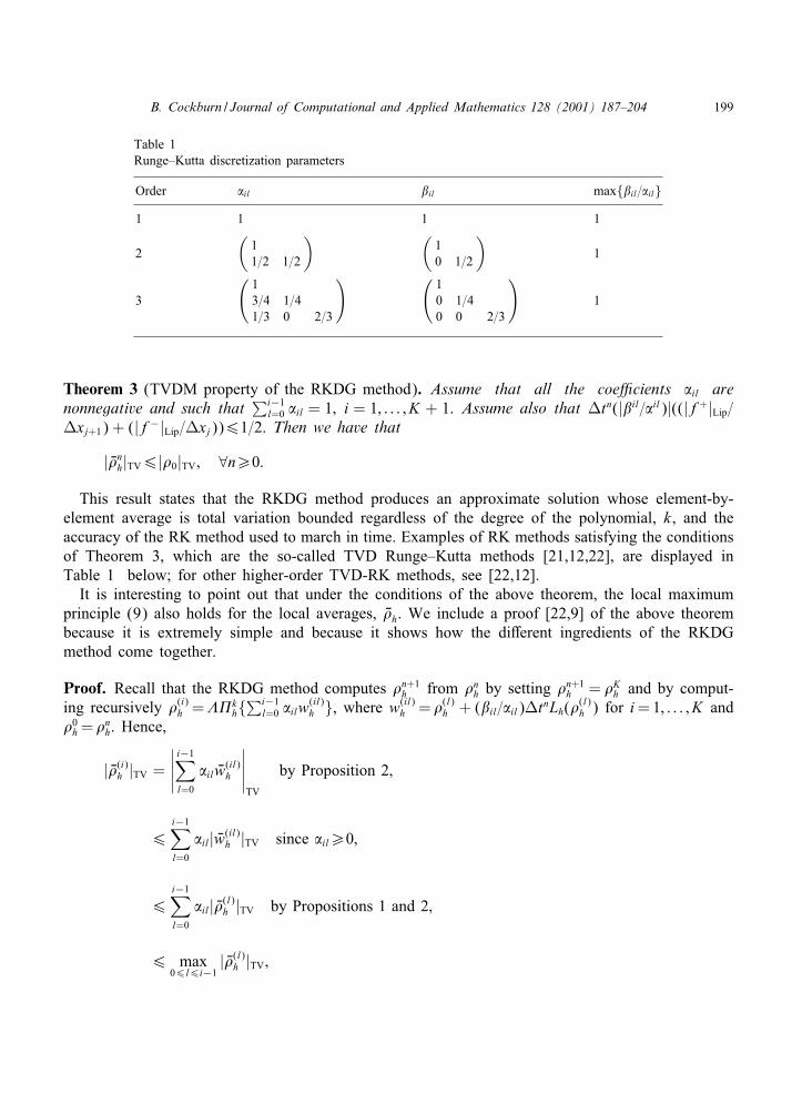
B. Cockburn / Journal of Computational and Applied Mathematics 128 (2001) 187–204 199
Table 1Runge–Kutta discretization parameters
Order �il 2il max{2il=�il}1 1 1 1
2
(11=2 1=2
) (10 1=2
)1
3
(13=4 1=41=3 0 2=3
) (10 1=40 0 2=3
)1
Theorem 3 (TVDM property of the RKDG method). Assume that all the coe5cients �il arenonnegative and such that
∑i−1l=0 �il = 1; i = 1; : : : ; K + 1. Assume also that Ptn(|2il=�il)|((|f+|Lip=
Pxj+1) + (|f−|Lip=Pxj))61=2. Then we have that
| S�nh|TV6|�0|TV; ∀n¿0:
This result states that the RKDG method produces an approximate solution whose element-by-element average is total variation bounded regardless of the degree of the polynomial, k, and theaccuracy of the RK method used to march in time. Examples of RK methods satisfying the conditionsof Theorem 3, which are the so-called TVD Runge–Kutta methods [21,12,22], are displayed inTable 1 below; for other higher-order TVD-RK methods, see [22,12].
It is interesting to point out that under the conditions of the above theorem, the local maximumprinciple (9) also holds for the local averages, S�h. We include a proof [22,9] of the above theorembecause it is extremely simple and because it shows how the di3erent ingredients of the RKDGmethod come together.
Proof. Recall that the RKDG method computes �n+1h from �n
h by setting �n+1h = �K
h and by comput-ing recursively �(i)
h =,-kh{∑i−1
l=0 �ilw(il)h }, where w(il)
h = �(l)h + (2il=�il)PtnLh(�
(l)h ) for i=1; : : : ; K and
�0h = �n
h. Hence,
| S�(i)h |TV =
∣∣∣∣∣i−1∑l=0
�il Sw(il)h
∣∣∣∣∣TV
by Proposition 2;
6i−1∑l=0
�il| Sw(il)h |TV since �il¿0;
6i−1∑l=0
�il| S�(l)h |TV by Propositions 1 and 2;
6 max06l6i−1
| S�(l)h |TV;

200 B. Cockburn / Journal of Computational and Applied Mathematics 128 (2001) 187–204
since∑i−1
l=0 �il =1. By induction, we get that | S�n+1h |TV6| S�n
h|TV, and so | S�nh|TV6| S�0
h|TV. Since �0h is the
L2-projection of �0, we have | S�0h|TV6|�0|TV, and the result follows.
4.2. Accuracy, convergence properties and some numerical results
Let us begin our discussion about the accuracy of the method by considering the linear casef′ constant. If we simply consider the DG space discretization and do not employ limiters, itcan be proven that when polynomials of degree k are used, the method is of order k + 1 in theL2-norm, uniformly in time, provided that the exact solution is smooth enough. If not a TVD-RKtime discretization of order k + 1 is used, there is ample numerical evidence that indicates that theaccuracy remains the same. When the complete RKDG method is used and the exact solution doesnot present any local critical points the accuracy is again of order k + 1. However, in the presenceof local critical points, the use of our limiter does degrade the order of accuracy. This happensbecause at those critical points, the approximation solution, which is a polynomial of degree k, isforcefully set equal to a constant by the limiter. Fortunately, this di5culty can be overcome bymeans of a slight modi=cation of the limiter ,-k
h- the resulting RKDG scheme can be proven tobe, not a TVDM scheme, but a total variation bounded in the means (TVBM) scheme; see [20,9].Moreover, the observed order of accuracy is now k+1. This has also been observed in all the mainprototypical nonlinear cases; see [9].
Now, let us address the issue of convergence to the entropy solution. From Theorem 3, it iseasy to see that the RKDG method (with the ,-k
h limiter or its TVBM modi1cation) generatesa subsequence that converges to a weak solution. However, unlike the case of the SCDG method,it has not been proven that such a weak solution is the entropy solution. Since all the numericalexperiments do indicate that this is actually the case, it is reasonable to expect that such a proofcould be obtained. This would require, however, new techniques; see [15,3,18].
Let us end this section by showing two numerical examples, both on the domain (0,1). The 1rstdeals with the simple, but numerically di5cult to approximate, linear case f(�) = � with initialcondition �0(x) = 1 if 0:4¡x¡ 0:6 and �0(x) = 0 otherwise. Our purpose is to illustrate how theamount of numerical dissipation varies with the polynomial degree k of the RKDG method; weuse our ,-k
h limiter. The results, for T = 100, are displayed in Fig. 2 where we see that thenumerical dissipation diminishes as the polynomial degree increases. The second example deals withthe classical inviscid Burgers equation f(�)=�2=2 with initial data �0(x)=0:25+0:5 sin(�(2x−1)).Our purpose is to display the performance of the RKDG method around the shock. We use a TVBMmodi1cation of our limiter which leaves untouched local critical points whose second-order derivativeis, in absolute value, smaller than M =20. In Fig. 3 we display how a shock passes through a singleelement. Note the excellent approximation to the exact solution only one element away form theexact shock for both k = 1 and 2.
5. Concluding remarks
The RKDG method has been extended to multidimensional nonlinear hyperbolic systemsand has proven to be a highly parallelizable, stable and accurate method. It has also been extendedto convection–di3usion equations, the Hamilton–Jacobi equations, nonlinear possibly degenerate
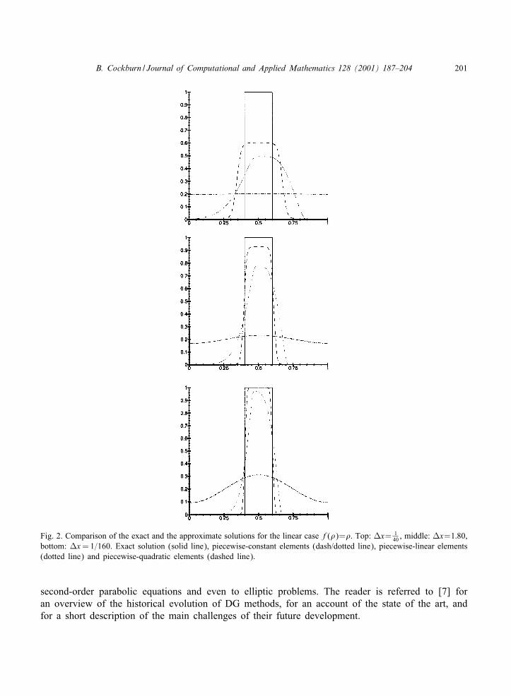
B. Cockburn / Journal of Computational and Applied Mathematics 128 (2001) 187–204 201
Fig. 2. Comparison of the exact and the approximate solutions for the linear case f(�)=�. Top: Px= 140 , middle: Px=1:80,
bottom: Px=1=160. Exact solution (solid line), piecewise-constant elements (dash/dotted line), piecewise-linear elements(dotted line) and piecewise-quadratic elements (dashed line).
second-order parabolic equations and even to elliptic problems. The reader is referred to [7] foran overview of the historical evolution of DG methods, for an account of the state of the art, andfor a short description of the main challenges of their future development.

202 B. Cockburn / Journal of Computational and Applied Mathematics 128 (2001) 187–204
Fig. 3. Comparison of the exact and the approximate solutions for the Burgers equation f(�) = �2=2; Px = 1=40 asthe shock passes through one element. Exact solution (solid line), piecewise linear elements (dotted line) and piecewisequadratic elements (dashed line). Top: T = 0:40, middle: T = 0:45, and bottom: T = 0:50.
Let us give an idea of the computational results this method produces and let us consider theclassical double Mach re/ection test problem. In Fig. 4, we display the results obtained by usingP2 polynomials on squares. Note the rich structure around the contact discontinuities that can be

B. Cockburn / Journal of Computational and Applied Mathematics 128 (2001) 187–204 203
Fig. 4. Approximate density obtained by the RKDG method.
captured because of the small amount of arti1cal dissipation (recall Fig. 2) and how sharply thestrong shocks have been approximated (recall Fig. 3).
In this paper we have tried to give a /avor of the techniques used to devise DG methods fornonlinear hyperbolic conservation laws in the framework of a one-dimensional scalar conservationlaw. Our main point is that the non-linear scalar conservation law obtained by dropping the term��xx from the equation de1nes an ill-posed problem and that the main e3ort to devise DG methodsfor the hyperbolic conservation law is to re-incorporate into the numerical scheme the informa-tion provided by the neglected term. We have seen that this can be accomplished by means of(i) approximate Riemann solvers and their corresponding numerical /uxes and by means of (ii)shock-capturing terms and generalized slope limiters. It is our hope that these ideas could be ofuse when devising DG methods for other nonlinear hyperbolic systems and even for more challeng-ing ill-posed problems like, for example, the model of phase transition in solids; see [4] and thereferences therein.
Acknowledgements
The author would like to thank Endre SWuli for the kind invitation to incorporate this paperinto this special volume of the Journal of Computational and Applied Mathematics. The authorwould also like to thank Franco Brezzi, Pierre A. Gremaud, Donatella Marini, K.W. Morton, PetrPlechXaYk, Chi-Wang Shu, and Endre SWuli for the many conversations this paper is the product of.
204 B. Cockburn / Journal of Computational and Applied Mathematics 128 (2001) 187–204
References
[1] B. Cockburn, An introduction to the discontinuous Galerkin method for convection-dominated problems, in:A. Quarteroni (Ed.), Advanced Numerical Approximation of Nonlinear Hyperbolic Equations, Lecture Notes inMathematics, Vol. 1697; Subseries Fondazione C.I.M.E., Firenze, Springer, Berlin, 1998, pp. 151–268.
[2] B. Cockburn, Discontinuous Galerkin methods for convection-dominated problems, in: T. Barth, H. Deconink (Eds.),High-Order Methods for Computational Physics, Lecture Notes in Computational Science and Engineering, Vol. 9,Springer, Berlin, 1999, pp. 69–224.
[3] B. Cockburn, F. Coquel, P. LeFloch, An error estimate for 1nite volume methods for multidimensional conservationlaws, Math. Comp. 63 (1994) 77–103.
[4] B. Cockburn, H. Gau, A model numerical scheme for the propagation of phase transitions in solids, SIAM J. Sci.Comput. 17 (1996) 1092–1121.
[5] B. Cockburn, P.A. Gremaud, Error estimates for 1nite element methods for nonlinear conservation laws, SIAM J.Numer. Anal. 33 (1996) 522–554.
[6] B. Cockburn, S. Hou, C.W. Shu, TVB Runge–Kutta local projection discontinuous Galerkin 1nite element methodfor conservation laws IV: the multidimensional case, Math. Comp. 54 (1990) 545–581.
[7] B. Cockburn, G.E. Karniadakis, C.-W. Shu (Eds.), First International Symposium on Discontinuous Galerkin Methods,Lecture Notes in Computational Science and Engineering, Vol. 11, Springer, Berlin, February 2000.
[8] B. Cockburn, S.Y. Lin, C.W. Shu, TVB Runge–Kutta local projection discontinuous Galerkin 1nite element methodfor conservation laws III: one dimensional systems, J. Comput. Phys. 84 (1989) 90–113.
[9] B. Cockburn, C.W. Shu, TVB Runge–Kutta local projection discontinuous Galerkin 1nite element method for scalarconservation laws II: general framework, Math. Comp. 52 (1989) 411–435.
[10] B. Cockburn, C.W. Shu, The Runge–Kutta local projection P1-discontinuous Galerkin method for scalar conservationlaws, RAIRO ModXel. Math. Anal. NumXer. 25 (1991) 337–361 .
[11] B. Cockburn, C.W. Shu, The Runge–Kutta discontinuous Galerkin 1nite element method for conservation laws V:Multidimensional systems, J. Comput. Phys. 141 (1998) 199–224.
[12] S. Gottlieb, C.-W. Shu, Total variation diminishing Runge–Kutta schemes, Math. Comp. 67 (1998) 73–85.[13] A. Harten, J.M. Hyman, P. Lax, On 1nite di3erence approximations and entropy conditions for shocks, Comm. Pure
Appl. Math. 29 (1976) 297–322.[14] A. Harten, P. van Leer, On upstream di3erencing and godunov-type schemes for hyperbolic conservation laws, SIAM
Rev. 25 (1983) 35–61.[15] G. Jiang, C.-W. Shu, On cell entropy inequality for discontinuous Galerkin methods, Math. Comp. 62 (1994) 531–
538.[16] C. Johnson, Adaptive 1nite element methods for conservation laws, in: A. Quarteroni (Ed.), Advanced Numerical
Approximation of Nonlinear Hyperbolic Equations, Lecture Notes in Mathematics, Vol. 1697; Subseries FondazioneC.I.M.E., Firenze, Springer, Berlin, 1998, pp. 269–323.
[17] K.W. Morton, Numerical Solution of Convection-Di3usion Problems, Chapman & Hall, London, 1996.[18] S. NWoelle, A note on entropy inequalities and error estimates for higher-order accurate 1nite volume schemes on
irregular families of grids, Math. Comp. 65 (1996) 1155–1163.[19] S. Osher, Riemann solvers, the entropy condition and di3erence approximations, SIAM J. Numer. Anal. 21 (1984)
217–235.[20] C.W. Shu, TVB boundary treatment for numerical solutions of conservation laws, Math. Comp. 49 (1987) 123–134.[21] C.-W. Shu, Essentially non-oscillatory and weighted essentially non-oscillatory schemes for hyperbolic conservation
laws, in: A. Quarteroni (Ed.), Advanced Numerical Approximation of Nonlinear Hyperbolic Equations, Lecture Notesin Mathematics, Vol. 1697, Subseries Fondazione C.I.M.E., Firenze, Springer, Berlin, 1998, pp. 325–432.
[22] C.-W. Shu, S. Osher, E5cient implementation of essentially non-oscillatory shock-capturing schemes, J. Comput.Phys. 77 (1988) 439–471.
[23] E. Tadmor, Approximate solutions of nonlinear conservation laws, in: A. Quarteroni (Ed.), Advanced NumericalApproximation of Nonlinear Hyperbolic Equations, Lecture Notes in Mathematics, Vol. 1697; Subseries FondazioneC.I.M.E., Firenze, Springer, Berlin, 1998, pp. 1–149.
[24] G.B. Witham, Linear and Nonlinear Waves, Wiley, New York, 1974.
Journal of Computational and Applied Mathematics 128 (2001) 205–233www.elsevier.nl/locate/cam
Adaptive Galerkin $nite element methods for partialdi%erential equations
R. RannacherInstitute of Applied Mathematics, University of Heidelberg, INF 293=294, D-69120 Heidelberg, Germany
Received 10 November 1999; received in revised form 28 February 2000
Abstract
We present a general method for error control and mesh adaptivity in Galerkin $nite element discretizations of partialdi%erential equations. Our approach is based on the variational framework of projection methods and uses concepts fromoptimal control and model reduction. By employing global duality arguments and Galerkin orthogonality, we derive aposteriori error estimates for quantities of physical interest. These residual-based estimates contain the dual solution andprovide the basis of a feed-back process for successive mesh adaptation. This approach is developed within an abstractsetting and illustrated by examples for its application to di%erent types of di%erential equations including also an optimalcontrol problem. c© 2001 Elsevier Science B.V. All rights reserved.
Keywords: Finite elements; Partial di%erential equations; Error control; Mesh adaptation; Model reduction; Optimalcontrol; Wave propagation
1. Introduction
Solving complex systems of partial di%erential equations by discretization methods may be con-sidered in the context of model reduction; a conceptually in$nite-dimensional model is approximatedby a $nite-dimensional one. As an example, we may think of a $nite volume or a Galerkin $niteelement method applied to compute the drag coe<cient of a body immersed in a viscous =uid wherethe governing continuous model is given by the classical Navier–Stokes equations. Here, the qualityof the approximation depends on the proper choice of the discretization parameters (the mesh width,the polynomial degree of the trial functions, the size of certain stabilization parameters, etc.). As theresult of the computation, we obtain an approximation to the desired output quantity of the simulationand besides that certain accuracy indicators like cell-truncation errors or cell-residuals. Controllingthe error in such an approximation of a continuous model of a physical system requires to determine
E-mail address: [email protected] (R. Rannacher).
0377-0427/01/$ - see front matter c© 2001 Elsevier Science B.V. All rights reserved.PII: S 0377-0427(00)00513-6

206 R. Rannacher / Journal of Computational and Applied Mathematics 128 (2001) 205–233
Fig. 1. Scheme of error propagation.
the in=uence factors for the local error indicators on the target functional. Such a sensitivity analysiswith respect to local perturbations of the model is common in optimal control theory and introducesthe notion of a dual (or adjoint) problem. It is used to describe the following two features of theapproximation process:
(i) Global error transport: The local error eK at some mesh cell K may be strongly a%ected bythe residuals �K′ at distant cells K ′ (so-called “pollution e%ect”).
(ii) Interaction of error components: The error in one component of the solution may depend onthe di%erent components of the cell-residuals in a complicated way.
An e%ective method for error estimation should take all these dependencies into account. The e%ectof the cell residuals �K on the local error components eK′ , at another cell K ′, is governed by theglobal Green tensor of the continuous problem. Capturing this dependence by numerical evaluationis the general philosophy underlying our approach to error control (Fig. 1).
The mechanisms of error propagation can be rather di%erent depending on the characteristics ofthe di%erential operator:
• Di%usion terms cause slow isotropic error decay, but global error pollution may occur from localirregularities.
• Advection terms propagate local errors in the transport direction, but errors decay exponentiallyin the crosswind direction.
• Reaction terms cause isotropic exponential error decay, but “sti% ” behavior may occur in thecoupling of error components.
For models in which all these mechanisms are present it is mostly impossible to determine thecomplex error interaction by analytical means, but rather has to be aided by computation. Thisautomatically leads to a feed-back process in which error estimation and mesh adaptation goeshand-in-hand leading to economical discretizations for computing the quantities of interest. Such anapproach seems indispensable for the numerical simulation of large-scale problems. It is particularlydesigned for achieving high solution accuracy at minimum computational costs.
Traditionally, a posteriori error estimation in Galerkin $nite element methods is done with respectto the natural energy norm induced by the underlying di%erential operator; for references see thesurvey articles by Ainsworth and Oden [1] and VerfKurth [22]. This approach seems rather generic asit is directly based on the variational formulation of the problem and allows to exploit its coercivityproperties. However, in most applications the error in the energy norm does not provide a usefulbound on the error in the quantities of real physical interest. A more versatile method for a posteriorierror estimation with respect to more relevant error measures (L2 norm, point values, line averages,etc.) is obtained by using duality arguments as common from a priori error analysis of $nite element
R. Rannacher / Journal of Computational and Applied Mathematics 128 (2001) 205–233 207
methods. This approach has $rst been systematically developed by Johnson and his co-workers[16,12] and was then extended by the author and his group to a practical feedback method for meshoptimization ([11,10]; see also [19] for a survey of this method). Below, we will describe this generalapproach to error control and adaptivity $rst within an abstract setting and then illustrate it by simpleexamples of its use for di%erent types of di%erential equations including also an optimal controlproblem. More involved applications have been considered by Becker [4,5] (viscous incompressible=ows), Becker et al. [6,7,3] (chemically reactive =ows), Kanschat [18] (radiative transfer), Rannacherand Suttmeier [20] (elasto-plasticity), Bangerth and Rannacher [3] (acoustic waves), and Beckeret al. [9] (optimal control).
2. A general paradigm for a posteriori error estimation
We present our approach to residual-based adaptivity in an abstract variational setting followingthe general paradigm described by Johnson [16] and Eriksson et al. [12]. For a detailed discussionof various aspects of this method, we refer to [11,10].
Let V be a Hilbert space with inner product (·; ·) and norm ‖·‖. Further, let A(·; ·) be a semi-linearform with derivatives A′(·; ·; ·) and A′′(·; ·; ·; ·) de$ned on V . We seek a solution u ∈ V to thevariational equation
A(u;’) = 0 ∀’ ∈ V: (1)
This problem is approximated by a Galerkin method using a sequence of $nite-dimensional subspacesVh⊂V , where h ∈ R+ is a discretization parameter.The discrete problems seek uh ∈ Vh satisfying
A(uh;’h) = 0 ∀’h ∈ Vh: (2)
The key feature of this approximation is the “Galerkin orthogonality” which in this nonlinear caseis expressed as
A(u;’h)− A(uh;’h) = 0; ’h ∈ Vh: (3)
Suppose that we want to bound the error E(uh) := J (u)−J (uh) with respect to some output functionalJ (·) de$ned on V with derivatives J ′(·; ·) and J ′′(·; ·; ·). For this situation, we have the followinggeneral result.
Proposition 1. For the Galerkin scheme (2) there holds in 7rst-order approximation the a posteriorierror estimate
|E(uh)| �(uh) := inf’h∈Vh
|A(uh; z − ’h)|; (4)
where z ∈ V is the solution of the linearized dual problem
A′(uh;’; z) = J ′(uh;’) ∀’ ∈ V: (5)
The a posteriori error estimate (4) becomes exact if the form A(·; ·) and the functional J (·) are(a;ne-) linear.
208 R. Rannacher / Journal of Computational and Applied Mathematics 128 (2001) 205–233
Proof. We set e := u− uh. By elementary calculus, there holds
A(u; ·) = A(uh; ·) + A′(uh; e; ·)−∫ 1
0A′′(uh + se; e; e; ·)(s− 1) ds;
J (u) = J (uh) + J ′(uh; e)−∫ 1
0J ′′(uh + se; e; e)(s− 1) ds:
Hence, setting ’= e in the dual problem (5), it follows that
E(uh) = J ′(uh; e)−∫ 1
0J ′′(uh + se; e; e)(s− 1) ds
=A′(uh; e; z)−∫ 1
0J ′′(uh + se; e; e)(s− 1) ds
=A(u; z)− A(uh; z) + r(e; e) (6)
with the remainder term
r(e; e) :=∫ 1
0{A′′(uh + se; e; e; z)− J ′′(uh + se; e; e)}(s− 1) ds:
Hence, using the Galerkin orthogonality (3) and that u solves (1), we $nd
E(uh) =−A(uh; z − ’h) + O(‖e‖2); (7)
provided that the second derivatives of A(·; ·) and J (·) are bounded and that also the dual solutionz is bounded uniformly with respect to h. Clearly, the O(‖e‖)2-term is not present if A(·; ·) and J (·)are (a<ne-) linear.
The a posteriori error estimate (4) holds in general only approximately due to the use of alinearized duality argument. Controlling the e%ect of this perturbation may be a delicate task and de-pends strongly on the particular problem considered. Our experiences with di%erent types of problems(including the Navier–Stokes equations and problems in elasto-plasticity) indicate that this problemis less critical as long as the continuous solution is stable. The crucial problem is the numericalcomputation of the linearized dual solution z by solving a discretized dual problem
A′(uh;’h; zh) = J ′(uh;’h) ∀’h ∈ Vh: (8)
This results in practically useful error estimators as we will see below.Next, we consider the special situation that the semi-linear form A(·; ·) is given as di%erential of
some “energy” functional L(·) on V , i.e., A(·; ·) = L′(·; ·). Then, the analogue of problem (1),
L′(u;’) = 0 ∀’ ∈ V; (9)
determines stationary points of L(·). Its Galerkin approximation reads
L′(uh;’h) = 0 ∀’h ∈ Vh: (10)
In this case the general a posteriori error estimate (4) takes the form
|E(uh)| inf’h∈Vh
|L′(uh; z − ’h)|: (11)
R. Rannacher / Journal of Computational and Applied Mathematics 128 (2001) 205–233 209
Now, we restrict the situation even more by taking the generating functional L(·) also for errorcontrol, i.e., we consider the error
E(uh) :=L(u)− L(uh):
We want to drive the corresponding analogue of the estimate (11).
Proposition 2. Suppose that the variational equation is derived from an “energy” functional L(·)and that the same functional is used for error control in the Galerkin method. In this case; thecorresponding linearized dual problem has the solution z=− 1
2e and the a posteriori error estimate(11) becomes
|E(uh)| �(uh) := inf’h∈Vh
12 |L′(uh; u− ’h)|: (12)
This error bound is exact if the functional L(·) is quadratic.
Proof. In virtue of the particular relations J (·)=L(·) and A(·; ·)=L′(·; ·), we can re$ne the argumentused in the proof of Proposition 1. First, integrating by parts and observing L′(u; ·) ≡ 0, we canwrite
E(uh) =∫ 1
0L′(uh + se; e) ds= L′(u; e)−
∫ 1
0L′′(uh + se; e; e) s ds
=−12L′′(uh; e; e) +
12
∫ 1
0L′′′(uh + se; e; e; e) (s2 − 1) ds;
with the third derivative L′′′(·; ·; ·; ·) of L(·). This suggests to work with the linearized dual problem
L′′(uh;’; z) =− 12L
′′(uh;’; e) ∀’ ∈ V; (13)
which has the solution z =− 12e. Further, noting again that L′(u; ·) ≡ 0, there holds
0 = L′(uh; z) + L′′(uh; e; z) +∫ 1
0L′′′(uh + se; e; e; z) (s− 1) ds:
From the foregoing relations, we conclude that
E(uh) = L′′(uh; e; z) +12
∫ 1
0L′′′(uh + se; e; e; e) (s2 − 1) ds
=−L′(uh; z)−∫ 1
0L′′′(uh + se; e; e; z)
{(s− 1) +
12(s2 − 1)
}ds:
Next, employing Galerkin orthogonality, there holds
L′(uh; z) = L′(uh; z − ’h); ’h ∈ Vh: (14)
Hence, recalling that z =− 12e, we conclude
|E(uh)|= inf’h∈Vh
12 |L′(uh; u− ’h)|+O(‖e‖3); (15)
where the O(‖e‖3) term vanishes if the functional L(·) is quadratic. This proves the assertion.

210 R. Rannacher / Journal of Computational and Applied Mathematics 128 (2001) 205–233
Again, in the a posteriori error estimate (12) the quantity u − ’h has to be approximated asdescribed above by using the computed solution uh ∈ Vh. We emphasize that in this particular casethe evaluation of the a posteriori error estimate with respect to the “energy” functional L(·) does notrequire the explicit solution of a dual problem. We will illustrate this general reasoning for somemodel situations below.
3. Evaluation of the a posteriori error estimates
The goal is to evaluate the right-hand side of (4) or (12) numerically, in order to get a criterionfor the local adjustment of the discretization. For the further discussion, we need to become morespeci$c about the setting of the variational problem. For example, let the variational problem (1)originate from a quasi-linear elliptic partial di%erential equation of the form
A(u) := −� · a(�u) = f; (16)
on a bounded domain �⊂Rd, with some f ∈ L2(�) and homogeneous Dirichlet boundary conditions,u|@� = 0. Let (·; ·)D denote the L2 scalar product on some domain D and ‖ · ‖D the correspondingnorm; in the case D=�, we will usually omit the subscript D. The function a :Rd → Rd is assumedto be su<ciently regular, such that the corresponding “energy” form
A(u;’) := (a(�u);�’)− (f;’)
and its derivative
A′(u;’; ) :=d∑
i=1
(a′(�u)�’;� );
are well de$ned on the Sobolev space V :=H 10 (�). The following discussion assumes (16) to be a
scalar equation, but everything carries directly over to systems.We consider the approximation of (16) by standard low-order conforming (linear or bilinear) $nite
elements de$ned on quasi-regular meshes Th = {K} consisting of non-degenerate cells K (trianglesor rectangles in two and tetrahedra or hexahedra in three dimensions) as described in the standard$nite element literature; see, e.g., [15]. The local mesh width is denoted by hK =diam(K). We alsouse the notation h= h(x) for a global mesh-size function de$ned by h|K ≡ hK . For the ease of localmesh re$nement and coarsening, we allow cells with “hanging nodes” as shown in Fig. 2.
In this setting, the error representation (11) can be developed into a more concrete form. Bycellwise integration by parts, we obtain
|E(uh)| |A(uh; z − ’h)|
6∑K∈Th
|(f − A(uh); z − ’h)K − 12 (n · [a(�uh)]; z − ’h)@K |;
with the corresponding dual solution z ∈ V and an arbitrary ’h ∈ Vh. Here, [a(�uh)] denotes thejump of the (generally discontinuous) =ux a(�uh) across the cell boundaries @K , with the convention[a(�uh)] := a(�uh) along @�.

R. Rannacher / Journal of Computational and Applied Mathematics 128 (2001) 205–233 211
Fig. 2. Q1 nodal basis function on a 2-d cell patch with hanging nodes.
Notice that in the nonlinear case, this error estimate only holds in $rst-order approximation; seeProposition 1. For later use in mesh adaptation algorithms, we write it in the form
|E(uh)|6�(uh) :=∑K∈Th
�K(uh); (17)
with the cellwise error indicators
�K(uh) := |(f − A(uh); z − ’h)K − 12 (n · [a(�uh)]; z − ’h)@K |:
The interpretation of this is as follows. On each cell, we have an “equation residual” f − A(uh)and a “=ux residual” n · [a(�uh)], the latter one expressing smoothness of the discrete solution.Both residuals can easily be evaluated. They are multiplied by the weighting function z−’h whichprovides quantitative information about the impact of these cell-residuals on the error E(uh) in thetarget quantity. In this sense z − ’h may be viewed as sensitivity factors like in optimal controlproblems. We recall the local approximation properties of $nite elements, in the present case oflinear or d-linear shape functions (for references see, e.g., [15]),
‖v− Ihv‖K + h1=2K ‖v− Ihv‖@K6cIh2K‖�2v‖K ; (18)
where Ih denotes the natural nodal interpolation operator, and cI is an interpolation constant usuallyof size cI ∼ 0:1–1. Hence, taking ’h = Ihz in (17), there holds
�K(uh)6�K(uh)!K(z); (19)
with the cell residuals
�K(uh) := ‖f − A(uh)‖K + 12h
−1=2K ‖n · [a(�uh)]‖@K ;
and the weights
!K(z) := cIh2K‖�2z‖K :Accordingly, the in=uence factors have the behavior h2K‖�2z‖K which is characteristic for the $niteelement approximation being a projection method. We note that for a 7nite di>erence discretization
212 R. Rannacher / Journal of Computational and Applied Mathematics 128 (2001) 205–233
which lacks the Galerkin orthogonality property the corresponding in=uence factors would behavelike ‖z‖K .
4. Algorithmic aspects of mesh adaptation
For evaluating the a posteriori error estimator � (uh), one may solve the linearized dual problemnumerically by the same method as used in computing uh yielding an approximation zh ∈ Vh,
A′(uh;’h; zh) = J ′(uh;’h) ∀’h ∈ Vh: (20)
However, the use of the same meshes for computing primal and dual solution is by no meansobligatory. In fact, for transport-dominated problems it may be advisable to compute the dual solutionon a di%erent mesh or with higher-order approximation; see [14,2,3] for examples.
There are various possibilities for evaluating the cell-error indicators �K(uh) and to use them forlocal mesh re$nement and as stopping criterion for the adaptation process.
4.1. Strategies for estimator evaluation
• Approximation by second-order di%erence quotients of the discrete dual solution zh ∈ Vh, e.g.,
!K(z)6cIh2K‖�2z‖K ≈ cIh2+d=2K |�2
h zh(xK)|; (21)
xK being the center point of K , where �2z is the tensor of second derivatives of z and �2h zh a
suitable di%erence approximation.• Computation of a discrete dual solution zh′ ∈ Vh′ in a richer space Vh′ ⊃Vh (e.g., on a $ner mesh
or using higher-order $nite elements) and setting, e.g.,
!K(z) ≈ ‖zh′ − Ihzh′‖K ; (22)
where Ihzh′ ∈ Vh is the generic nodal interpolation.• Interpolation of the discrete dual solution zh ∈ Vh by higher-order polynomials on certain cell-patches, e.g., bi-quadratic interpolation I (2)h zh:
!K(z) ≈ ‖I (2)h zh − zh‖K : (23)
The second option is quite expensive and rarely used. Notice that the third option does notinvolve an interpolation constant which needs to be speci$ed. Our experience is that the use ofbi-quadratic interpolation on patches of four quadrilaterals is more accurate than using the $nitedi%erence approximation (21). One may try to further improve the quality of the error estimateby solving local (patchwise) defect equations, either Dirichlet problems (Qa la BabuRska and Miller)or Neumann problems (Qa la Bank and Weiser); for details see [11]. General references for theseapproaches are Ainsworth and Oden [1] and VerfKurth [22].
4.2. Strategies for mesh adaptation
The mesh design strategies are oriented towards a prescribed tolerance TOL for the error quantityE(uh)=J (u)−J (uh) and the number of mesh cells N which measures the complexity of the reduced
R. Rannacher / Journal of Computational and Applied Mathematics 128 (2001) 205–233 213
computational model. Usually the admissible complexity is constrained by some maximum valueNmax.
• Error balancing strategy: Cycle through the mesh and seek to equilibrate the local error indicators,
�K(uh) ≈ TOLN
: (24)
This process requires iteration with respect to the number of mesh cells N and eventually leadsto � (uh) ≈ TOL.• Fixed fraction strategy: Order cells according to the size of �K(uh) and re$ne a certain percentage(say 20%) of cells with largest �K(uh) (or those which make up 20% of the estimator value � (uh))and coarsen those cells with smallest �K(uh). By this strategy, we may achieve a prescribed rateof increase of N (or keep it constant in solving nonstationary problems).
• Mesh optimization strategy: Use the error representation
� (uh) ≈∑K∈Th
�K (uh) (25)
directly for generating a formula for an optimal mesh-size function hopt(x).
We want to discuss the “mesh optimization strategy” in more detail. As a by-product, we will alsoobtain the justi$cation of the indicator equilibration strategy. Let Nmax and TOL be prescribed. Weassume that for h→ 0, the normalized cell residuals approach certain mesh-independent limits,
h−d=2K �K (uh) ≈ $u(xK); (26)
which involve the second derivatives of the solution and the data. This property can rigorouslybe proven on uniformly re$ned meshes by exploiting super-convergence e%ects, but they still needtheoretical justi$cation on locally re$ned meshes as constructed by the strategies described above.For the weights, we know from (21) that
h−d=2−2K !K(z)6cI |�2z(xK)|=:$z(xK): (27)
This suggest to use the relation
� (uh) ≈ E(h) :=∫�h(x)2$(x) dx; (28)
with the mesh-independent function $(x) =$u(x)$z(x).
Proposition 3. Suppose that in the limit TOL → 0 or Nmax → 0 the error estimator takes on theform (28); and let
W :=∫�$(x)d=(2+d) dx¡∞: (29)
(I) The optimization problem E(h)→ min!; N6Nmax, has the solution
hopt(x) ≈(
WNmax
)1=d$(x)−1=(2+d): (30)
214 R. Rannacher / Journal of Computational and Applied Mathematics 128 (2001) 205–233
(II) The optimization problem N → min!; E(h)6TOL; has the solution
hopt(x) ≈(TOLW
)1=d$(x)−1=(2+d): (31)
Proof. First, we note the crucial relation
N (h) =∑K∈Th
hdKh
−dK ≈
∫�h(x)−d dx: (32)
Then with the Lagrangian functional
L(h; ') :=E(h) + '{N (h)− Nmax};the $rst-order optimality condition is
ddt
L(h+ t’; '+ t))|t=0 = 0;
for all admissible variations ’ and ). This implies that
2h(x)$(x)− d'h(x)−d−1 = 0;∫�h(x)−d dx − Nmax = 0:
Consequently,
h(x) =(
2d'
$(x))−1=(2+d)
;(
2d'
)d=(2+d) ∫�$(x)d=(2+d) dx = Nmax:
From this, we conclude the desired relations
' ≡ 2d
$(x)h(x)2+d
; hopt(x) =(
WNmax
)1=d$(x)−1=(2+d):
In an analogous way, we can also treat the optimization problem (II).
We note that even for rather “irregular” functionals J (·) the quantity W is bounded. For example,the evaluation of derivative point values J (u) = @iu(a) for smooth u in two dimensions leads to$(x) ≈ |x − a|−3 and, consequently,
W ≈∫�|x − a|−3=2 dx¡∞:
The explicit formulas for hopt(x) have to be used with care in designing a mesh. Their derivationimplicitly assumes that they actually correspond to scalar mesh-size functions of isotropic meshessuch that hopt|K ≈ hK . However, this condition is not incorporated into the formulation of themesh-optimization problems (I) and (II). Anisotropic meshes containing stretched cells require amore involved concept of mesh description and optimization. This is subject of current research.
5. A nested solution approach
For solving a nonlinear problem like (16) by the adaptive Galerkin $nite element method (2),we may employ the following scheme. Let a desired error tolerance TOL or a maximum mesh

R. Rannacher / Journal of Computational and Applied Mathematics 128 (2001) 205–233 215
complexity Nmax be given. Starting from a coarse initial mesh T0, a hierarchy of successively re$nedmeshes Ti ; i¿1, and corresponding $nite element spaces Vi is generated as follows:(0) Initialization i = 0: Compute an initial approximation u0 ∈ V0.(i) Defect correction iteration: For i¿1, start with u(0)i := ui−1 ∈ Vi.(ii) Iteration step: For j¿0 evaluate the defect
(d( j)i ; ’) :=F(’)− A(u( j)i ;’); ’ ∈ Vi: (33)
Choose a suitable approximation A′(u( j)i ; ·; ·) to the derivative A′(u( j)i ; ·; ·) (with good stability and
solubility properties) and compute a correction v( j)i ∈ Vi from the linear equation
A′(u( j)i ; v( j)i ; ’) = (d( j)
i ; ’) ∀’ ∈ Vi:
For this, Krylov-space or multi-grid methods are employed using the hierarchy of meshes {Ti ; : : : ;T0}.Then, update u( j+1)
i = u( j)i + 'iv( j)i , with some relaxation parameter 'i ∈ (0; 1], set j := j + 1 and go
back to (2). This process is repeated until a limit u i ∈ Vi, is reached with a certain prescribedaccuracy.
(iii) Error estimation: Accept u i =ui as the solution on mesh Ti and solve the discrete linearizeddual problem
zi ∈ Vi : A′(ui;’; zi) = J ′(ui;’) ∀’ ∈ Vi;
and evaluate the a posteriori error estimate
|E(ui)| ≈ �(ui): (34)
For controlling the reliability of this bound, i.e., the accuracy in the determination of the dualsolution z, one may check whether ‖zi − zi−1‖ is su<ciently small; if this is not the case, additionalglobal mesh re$nement is advisable. If �(ui)6TOL or Ni¿Nmax, then stop. Otherwise, cell-wisemesh adaptation yields the new mesh Ti+1. Then, set i := i + 1 and go back to (i).We note that the evaluation of the a posteriori error estimate (34) involves only the solution
of linearized problems. Hence, the whole error estimation may amount only to a relatively smallfraction of the total cost for the solution process. This has to be compared to the usually muchhigher cost when working on non-optimized meshes.
In using the a posteriori error estimate (34), it is assumed that the exact discrete solution ui ∈ Vi
on mesh Ti is available. This asks for estimation of the unavoidable iteration error u i − ui andits e%ect on the accuracy of the estimator for the discretization error. This can be achieved in thecase of a Galerkin $nite-element multigrid iteration by exploiting the projection properties of thecombined scheme; for details see [8].
6. Applications to model problems
6.1. An elliptic model problem
We begin with the Poisson di%usion problem
−Vu= f in �; u= 0 on @�; (35)

216 R. Rannacher / Journal of Computational and Applied Mathematics 128 (2001) 205–233
posed on a polygonal domain �⊂R2. In this case the “energy” form is de$ned by A(·; ·) := (�·;�·)− (f; ·) and the discrete problems read
(�uh;�’h) = (f;’h) ∀’h ∈ Vh: (36)
Here, Vh⊂V :=H 10 (�) are the $nite element subspaces as de$ned above. Now, let J (·) be an
arbitrary linear error functional de$ned on V and z ∈ V the solution of the corresponding dualproblem
(�’;�z) = J (’) ∀’ ∈ V: (37)
From the general a posteriori error estimate (17), we infer the following result.
Proposition 4. For the approximation of the Poisson problem (35) by the 7nite element scheme(36); there holds the a posteriori error estimate
|J (e)|6�(uh) :=∑K∈Th
{∑i=1;2
�(i)K (uh)!
(i)K (z)
}; (38)
where the cellwise residuals and weights are de7ned by
�(1)K (uh) := ‖f +Vuh‖K ; !(1)
K (z) := ‖z − Ihz‖K ;�(2)K (uh) := 1
2h−1=2K ‖n · [�uh]‖@K ; !(2)
K (z) := h1=2K ‖z − Ihz‖@K ;with some nodal interpolation Ihz ∈ Vh of z.
Example 1. We want to use Proposition 4 to derive an a posteriori bound for the L2-error. Usingthe functional J (’) := ‖e‖−1(e; ’) in the dual problem, we obtain the estimate
J (e) = ‖e‖6∑K∈Th
{∑i=1;2
�(i)K (uh)!
(i)K (z)
}: (39)
In view of the interpolation property (18) the weights my be estimated by
!(i)K (z)6cIh2K‖�2z‖2K :
This results in the error bound
‖e‖6 cI∑K∈Th
h2K
{∑i=1;2
�(i)K (uh)
}‖�2z‖K
6 cI
∑
K∈Th
h4K
{∑i=1;2
�(i)K (uh)
}21=2
‖�2z‖:
In view of the a priori bound ‖�2z‖6cS (cS =1 if � is convex), this implies the a posteriori errorestimate
‖e‖6�L2 (uh) := cIcS
∑
K∈Th
h4K
{∑i=1;2
�(i)K (uh)
}21=2
; (40)
which is well-known from the literature; see e.g., [12] or [22].
R. Rannacher / Journal of Computational and Applied Mathematics 128 (2001) 205–233 217
Example 2. We now consider a highly localized error functional. As concrete example, we choosethe square domain � = (−1; 1)2 and the error functional
J (u) = @1u(a)
at the mid point a=(0; 0). In this case, the dual solution does not exist in the sense of H 10 (�), such
that for practical use, we have to regularize the functional J (u) = @1u(a), for example like
J-(u) := |B-|−1∫B-
@1u dx = @1u(a) + O(-);
where B- = {x ∈ �| |x− a|¡-}, and - :=TOL is a suitable error tolerance. The corresponding dualsolution z behaves like
|�2z(x)| ≈ d(x)−3; d(x) := |x − a|+ -:
From the general a posteriori error estimate (38), we obtain for the present case
|@1e(a)| ≈ �(uh) := cI∑K∈Th
h3Kd3
K
{∑i=1;2
�(i)K (uh)
}: (41)
Now, we want to apply Proposition 3 for determining a priori an optimal meshsize distribution. Tothis end, let us again assume that the residuals behave like h−1
K {�(1)K (uh) + �(2)
K (uh)} ≈ $u(xK), witha mesh-independent function $u, such that
�(uh) ≈∫�h(x)2$(x)dx; $(x) :=
$u(x)d(x)3
:
Hence, from Proposition 3, we obtain
hopt(x) ≈(
WNmax
)1=2$(x)−1=4 ≈ Nmaxd(x)−3=4;
with W :=∫� $u(x)1=2dx¡∞. This implies the relation
Nopt =∑K∈Th
h2Kh−2K =
(Nopt
TOL
)1=2 ∑K∈Th
h2Kd−3=2K ≈
(Nopt
TOL
)1=2:
and, consequently, Nopt ≈ TOL−1. This is better than what could be achieved on uniformly re$nedmeshes. In fact, mesh re$nement on the basis of global energy-error control results in almost uniformre$nement, i.e., Nopt ≈ TOL−2. This predicted asymptotic behavior is well con$rmed by the resultsof our computational test. Fig. 3 shows the balanced mesh for TOL= 4−4 and the approximation tothe dual solution z-; - = TOL, computed on this mesh. The corresponding errors for a sequence oftolerances are listed in Table 1. For the problem considered, the weighted a posteriori estimate (38)for the point error is obviously asymptotically optimal and the predicted dependence Nopt ≈ TOL−1
is con$rmed; for more details, we refer to [11].

218 R. Rannacher / Journal of Computational and Applied Mathematics 128 (2001) 205–233
Fig. 3. Re$ned mesh and approximate dual solution for computing @1u(0) in Example 2, using the a posteriori errorestimator �(uh), with TOL = 4−4.
Table 1Results for computing @1u(0) using the a posteriori error estimator �(uh) for several levels ofre$nement L; the “e%ectivity index” is de$ned by Ie% := |@1e(0)|=�(uh)
TOL N L |@1e(0)| �(uh) Ie%
4−2 148 6 7:51e− 1 5:92e− 2 12.694−3 940 9 4:10e− 1 1:42e− 2 28.874−4 4912 12 4:14e− 3 3:50e− 3 1.184−5 20 980 15 2:27e− 4 9:25e− 4 0.244−6 86 740 17 5:82e− 5 2:38e− 4 0.24
Example 3. The third example is meant as an illustrative exercise. For problem (35) on a smoothlybounded domain �⊂R2, we consider the functional
J (u) :=∫@�
@nu ds(=∫�f dx
);
and pose the question: What is an optimal mesh-size distribution for computing J (u)? The answeris based on the observation that the corresponding dual problem
(�’;�z) =∫@�
@n’ ds ∀’ ∈ V ∩W 2;1(�);
has a measure solution with density of the form z ≡ 1 in �, z=0 on @�. In order to avoid the useof measures, we consider the regularized functional
J-(’) = |S-|−1∫S-@n’ dx =
∫@�
@n’ ds+O(-);
where -=TOL, S- := {x ∈ �; dist{x; @�}¡-}, and @n’ the generic continuation of @n’ to S-. Thecorresponding regularized dual solution is
z- = 1 in � \ S-; z-(x) = -−1dist{x; @�} on S-:
R. Rannacher / Journal of Computational and Applied Mathematics 128 (2001) 205–233 219
This implies that
J-(e)6cI∑
K∈Th; K∩S- �=∅h2K
{∑i=1;2
�(i)K (uh)
}‖�2z-‖K ;
i.e., there is no contribution to the error from the interior of �. Hence, independent of the form ofthe forcing f, the optimal strategy is to re$ne the elements adjacent to the boundary and to leavethe others unchanged, assuming of course, that the force term f is integrated exactly.
Example 4. Finally, we apply the abstract theory developed above to derive an “energy-norm” errorestimate. This is intended to prepare for the application to error estimation in approximating optimalcontrol problems.
The solution u ∈ V of (35) minimizes the quadratic “energy” functional
L(u) := 12‖�u‖2 − (f; u);
on the function space V = H 10 (�), i.e.,
L′(u; ’) = (�u;�’)− (f;’) = 0; ’ ∈ V: (42)
Further, we note that
L(u)− L(uh) = 12‖�u‖2 − (f; u)− 1
2‖�uh‖2 + (f; uh)
=− 12‖�u‖2 − 1
2‖�uh‖2 + (�u;�uh)
=− 12‖�e‖2:
Hence, energy-error control means control of the error with respect to the “energy” functional L(·).Applying Proposition 2 to this situation, we obtain the a posteriori error estimate
|L(u)− L(uh)|6 inf’h∈Vh
12 |L′(uh; u− ’h)| (43)
6∑K∈Th
{∑i=1;2
�(i)K (uh)!
(i)K (u)
}: (44)
which is exact since the functional L(·) is quadratic. Then, using the local approximation estimate(see, e.g., [22])
inf’h∈Vh
( ∑K∈Th
{h−2K ‖u− ’h‖2K + h−1
K ‖u− ’h‖2@K})1=26cI‖�e‖; (45)
we conclude that
|L(u)− L(uh)|6cI
∑
K∈Th
{∑i=1;2
�(i)K (uh)
}21=2
‖�e‖: (46)
220 R. Rannacher / Journal of Computational and Applied Mathematics 128 (2001) 205–233
This implies the standard energy-norm a posteriori error estimate (see, e.g., [22] or [1])
‖�e‖62cI
∑
K∈Th
{∑i=1;2
�(i)K (uh)
}21=2
: (47)
6.2. A nonlinear test case: Hencky model in elasto-plasticity
The results in this section are taken from Suttmeier [21] and Rannacher and Suttmeier [20].The fundamental problem in the static deformation theory of linear-elastic perfect-plastic material(so-called Hencky model) reads
� · / =−f; -(u) = A : / + ' in �;
' : (0− /)60 ∀0 with F(0)60;
u= 0 on 1D; / · n= g on 1N ;
(48)
where / and u are the stress tensor and displacement vector, respectively, while ' denotes the plasticgrowth. This system describes the deformation of an elasto-plastic body occupying a bounded domain�⊂Rd (d=2 or 3) which is $xed along a part 1D of its boundary @�, under the action of a bodyforce with density f and a surface traction g along 1N = @� \ 1D. The displacement u is supposedto be small in order to neglect geometric nonlinear e%ects, so that the strain tensor can be writtenas -(u)= 1
2(�u+�uT). The material tensor A is assumed to be symmetric and positive de$nite. Weassume a linear-elastic isotropic material law /=2)-D(u)+3� ·uI , with material-dependent constants)¿ 0 and 3¿ 0, while the plastic behavior follows the von Mises =ow rule F(/) := |/D| − /060,with some /0 ¿ 0. Here, -D and /D denote the deviatoric parts of - and /, respectively.The primal variational formulation of problem (48) seeks a displacement u ∈ V := {u ∈ H 1(�)d,
u|1D = 0}, satisfyingA(u;’) = 0 ∀’ ∈ V; (49)
with the semi-linear form
A(u;’) := (5(2)-D(u)); -(’)) + (3� · u;� · ’)− (f;’)− (g; ’)1N ;
and the projection
5(2)-D(u)) :=
2)-D(u) if |2)-D(u)|6/0;/0
|-D(u)|-D(u) if |2)-D(u)|¿/0:
The $nite element approximation of problem (49) reads
A(uh;’h) = 0 ∀’h ∈ Vh; (50)
where Vh is the $nite element space of bilinear shape functions as descibed above. Having computedthe displacement uh, we obtain a corresponding stress by /h :=5(2)-D(uh))+3� ·uhI . Details of thesolution process can be found in [21,20]. Given an error functional J (·), we may apply the generala posteriori error estimate (17) to the present situation.
R. Rannacher / Journal of Computational and Applied Mathematics 128 (2001) 205–233 221
Proposition 5. For the approximation of the Hencky model (48) by the 7nite element scheme (50);there holds the a posteriori error estimate
|J (e)|6∑K∈Th
{∑i=1;2
�(i)K (uh)!
(i)K (z)
}; (51)
where the cellwise residuals and weights are de7ned by
�(1)K (uh) := ‖f −� · C(-(uh))‖K ; !(1)
K (z) := ‖z − Ihz‖K ;�(2)K (uh) := 1
2h−1=2K ‖n · [C(-(uh))]‖@K ; !(2)
K (z) := h−1=2K ‖z − Ihz‖@K ;
with C(-) :=5(2)-D) + 3 tr(-) and some nodal interpolation Ihz ∈ Vh of z.
We compare the weighted error estimate (51) with two heuristic ways of estimating the stress errore/ :=/ − /h:(1) The heuristic ZZ-error indicator of Zienkiewicz and Zhu (see [1]) uses the idea of higher-order
stress recovery by local averaging,
‖e/‖ ≈ �ZZ(uh) :=
(∑K∈Th
‖Mh/h − /h‖2K)1=2
; (52)
where Mh/h is a local (super-convergent) approximation of /.(2) The heuristic energy error estimator of Johnson and Hansbo [17] is based on a decomposed of
the domain � into “discrete” plastic elastic zones, �=�ph ∪�e
h. Accordingly the error estimatorhas the form
‖e/‖ ≈ �E(uh) := cI
(∑K∈Th
�2K
)1=2; (53)
with the local error indicators de$ned by
�K(uh)2 :=
h2K{�(1)K (uh) + �(2)
K (uh)}2 if K ⊂�eh;
{�(1)K (uh) + �(2)
K (uh)}‖Mh/h − /h‖K if K ⊂�ph:
6.2.1. Numerical testA geometrically two-dimensional square disc with a hole is subjected to a constant boundary
traction acting upon two opposite sides. We use the two-dimensional plain-strain approximation, i.e.,the components of -(u) in z-direction are assumed to be zero. In virtue of symmetry the considerationcan be restricted to a quarter of the domain shown in Fig. 4; for the precise parameters in this modelsee [20]. Among the quantities to be computed is the component /22 of the stress tensor at point a2.The result on a very $ne adapted mesh with about 200,000 cells is taken as reference solution uref .
The result of this benchmark computation is summarized in Fig. 5. We see that the weighted aposteriori error estimate leads to more economical meshes, particularly if high accuracy is required.For more details as well as for further results also for the time-dependent. Prandtl–Reuss model inperfect plasticity, we refer to [20].
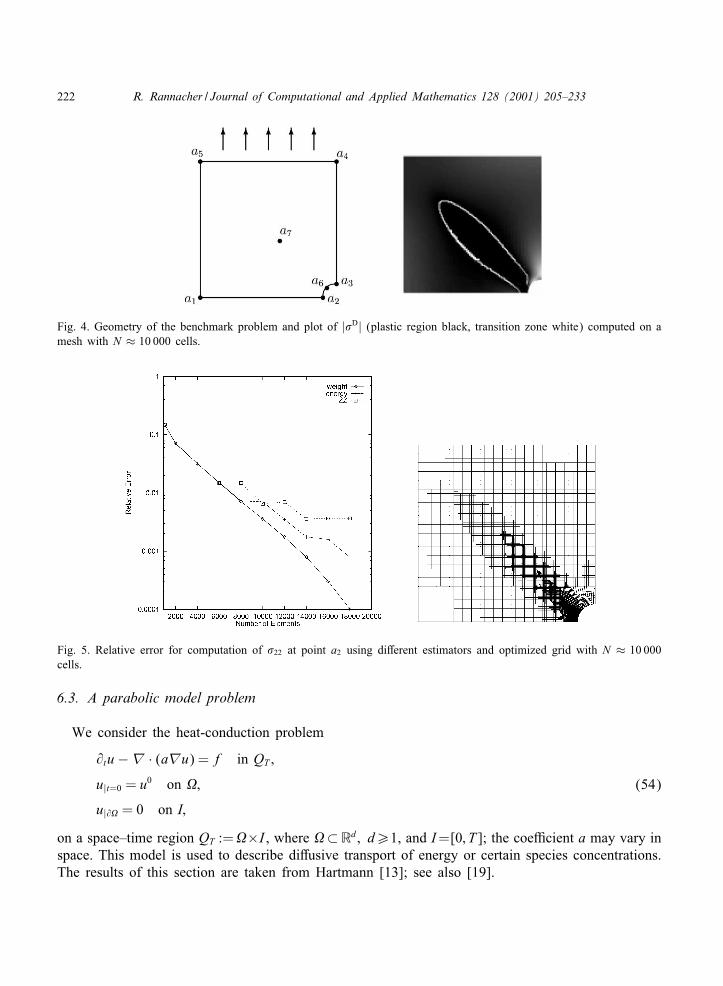
222 R. Rannacher / Journal of Computational and Applied Mathematics 128 (2001) 205–233
Fig. 4. Geometry of the benchmark problem and plot of |/D| (plastic region black, transition zone white) computed on amesh with N ≈ 10 000 cells.
Fig. 5. Relative error for computation of /22 at point a2 using di%erent estimators and optimized grid with N ≈ 10 000cells.
6.3. A parabolic model problem
We consider the heat-conduction problem
@tu−� · (a�u) = f in QT ;
u|t=0 = u0 on �;
u|@� = 0 on I;
(54)
on a space–time region QT :=�×I , where �⊂Rd; d¿1, and I=[0; T ]; the coe<cient a may vary inspace. This model is used to describe di%usive transport of energy or certain species concentrations.The results of this section are taken from Hartmann [13]; see also [19].

R. Rannacher / Journal of Computational and Applied Mathematics 128 (2001) 205–233 223
The discretization of problem (54) is by a Galerkin method in space–time. We split the timeinterval [0; T ] into subintervals In = (tn−1; tn] according to
0 = t0 ¡ · · ·¡tn ¡ · · ·¡tN = T; kn := tn − tn−1:
At each time level tn, let Tnh be a regular $nite element mesh as de$ned above with local mesh
width hK =diam(K), and let V nh ⊂H 1
0 (�) be the corresponding $nite element subspace with d-linearshape functions. Extending the spatial mesh to the corresponding space–time slab �× In, we obtaina global space–time mesh consisting of (d+ 1)-dimensional cubes Qn
K :=K × In. On this mesh, wede$ne the global $nite element space
V kh := {v ∈ W; v(·; t)|Qn
K∈ Q1(K); v(x; ·)|Qn
K∈ Pr(In);∀Qn
K};where W :=L2((0; T );H 1
0 (�)) and r¿0. For functions from this space and their time-continuousanalogues, we use the notation
vn+ := limt→tn+0
v(t); vn− := limt→tn−0
v(t); [v]n := vn+ − vn−:
The discretization of problem (54) is based on a variational formulation which allows the useof piecewise discontinuous functions in time. This method, termed “dG(r) method” (discontinuousGalerkin method in time), determines approximations uh ∈ V k
h by requiring
A(uh; ’h) = 0 ∀’h ∈ V kh ; (55)
with the semi-linear form
A(u; ’) :=N∑
n=1
∫In{(@tu; ’) + (a�u;�’)− (f;’)} dt +
N∑n=1
([u]n−1; ’+n−1);
where u−0 := u0. We note that the continuous solution u also satis$es equation (55) which againimplies Galerkin orthogonality for the error e := u−uh with respect to the bilinear form A(·; ·). Sincethe test functions ’h ∈ V k
h may be discontinuous at times tn, the global system (55) decouples andcan be written in form of a time-stepping scheme,∫
In{(@tuh; ’h) + (a�uh;�’h)} dt + ([uh]
n−1; ’(n−1)+h ) =
∫In(f;’h) dt;
for all ’h ∈ V nh ; n = 1; : : : ; N . In the following, we consider only the lowest-order case r = 0, the
“dG(0) method” which is equivalent to the backward Euler scheme. We concentrate on the controlof the spatial L2-error ‖eN−‖ at the end time T = tN . To this end, we use a duality argument inspace–time,
@tz − aVz = 0 in � × I;
z|t=T = ‖eN−‖−1eN− in �; z|@� = 0 on I;(56)
which can also be written in variational form as
A(’; z) = J (’) := ‖eN−‖−1(’N−; eN−) ∀’ ∈ W: (57)
Then, from Proposition 1, we obtain the estimate
‖eN−‖6N∑
n=1
∑K∈Tn
h
|(R(uh); z − ’h)K×In −12(n · [a�uh]; z − ’h)@K×In − ([uh]
n−1; (z − ’h)(n−1)+)K |;

224 R. Rannacher / Journal of Computational and Applied Mathematics 128 (2001) 205–233
with the residual R(uh) :=f +� · (a�uh)− @tuh and a suitable approximation ’h ∈ V kh to the dual
solution z. From this, we infer the following result.
Proposition 6. For the dG(0) 7nite element method applied to the heat conduction equation (54);there holds the a posteriori error estimate
‖eN+‖6N∑
n=1
∑K∈Tn
h
{∑i=1;2;3
�n; iK (uh)!
n; iK (z)
}; (58)
where the cellwise residuals and weights are de7ned by
�n;1K (uh) := ‖R(uh)‖K×In ; !n;1
K (z) := ‖z − I kh z‖K×In ;
�n;2K (uh) := 1
2h−1=2K ‖n · [a�uh]‖@K×In ; !n;2
K (z) := h1=2K ‖z − I kh z‖@K×In ;
�n;3K (uh) := k−1=2
n ‖[uh]n−1‖K ; !n;3K (z) := k1=2
n ‖(z − I kh z)(n−1)+‖K :
with some nodal interpolation I kh z ∈ Wh of z.
The weights are evaluated numerically as described in Section 3 above.
6.3.1. Numerical testThe performance of the error estimator (58) is illustrated by a simple test in two space dimensions
where the (known) exact solution represents a smooth rotating bump with a suitably adjusted forcef on the unit square; for details see [13]. Fig. 6 shows a sequence of adapted meshes at successivetimes obtained by controlling the spatial L2 error at the end time tN = 0:5. We clearly see the e%ectof the weights in the error estimator which suppress the in=uence of the residuals during the initialperiod.
6.4. A hyperbolic model problem
We consider the acoustic wave equation
@2t u−� · {a�u}= 0 in QT ;
u|t=0 = u0; @tu|t=0 = v0 on �;
n · a�u|@� = 0 on I;
(59)
on a space–time region QT :=� × I , where �⊂Rd; d¿1, and I = [0:T ]; the elastic coe<cient amay vary in space. This equation frequently occurs in the simulation of acoustic waves in gaseousor =uid media, seismics, electro-dynamics and many other applications. The material of this sectionis taken from Bangerth [2] and Bangerth and Rannacher [3].
We approximate problem (59) by a “velocity-displacement” formulation which is obtained byintroducing a new velocity variable v := @tu. Then, the pair w= {u; v} satis$es the linear variationalequation
A(w; �) = 0 ∀� = {’; } ∈ T; (60)

R. Rannacher / Journal of Computational and Applied Mathematics 128 (2001) 205–233 225
Fig. 6. Sequence of re$ned meshes at time tn = 0:125; 0:421875; 0:5, for controlling the end-time error ‖eN−‖.
with the bilinear form
A(w; �) := (@tu; ’)QT − (v; ’)QT + (@tv; )QT + (a�u;� )QT ;
and a suitable space T of test functions � for which A(w; �) is de$ned. This formulation is the basisfor a Galerkin discretization in space–time similar to the one described in the preceding sectionfor the heat-conduction equation. We decompose the time interval I = [0; T ] again into subintervalsIn=(tn−1; tn] with length kn= tn− tn−1. On each time slab Qn :=�× In, we use meshes Tn
h consistingof (d + 1)-dimensional cubes Qn
K = K × In with spatial width hK ; these meshes may vary betweenthe time levels in order to allow for grid re$nement moving with the wave $eld. The discrete “trialspaces” Wh = Vh × Vh in space–time domain consist of functions which are (d + 1)-linear on eachspace–time cell Qn
K and globally continuous on QT . This prescription requires the use of “hangingnodes” if the spatial mesh changes across a time level tn. The corresponding discrete “test spaces”Th⊂T consist of functions which are constant in time on each cell Qn
K , while they are d-linearin space and globally continuous on �. We further assume that the test space T is chosen largeenough to contain the elements from w + Wh. The Galerkin approximation of problem (59) seekspairs wh = {uh; vh} ∈ Wh satisfying
A(wh; �h) = 0 ∀�h = {’h; h} ∈ Th: (61)
For more details, we refer to [2,3]. Since the continuous solution w also satis$es (61), we haveagain Galerkin orthogonality for the error e := {eu; ev}. This time-discretization scheme is termed“cG(1)-method” (continuous Galerkin method) in contrast to the dG-method used in the precedingsection. We note that from this scheme, we can recover the standard Crank–Nicolson scheme intime combined with a spatial $nite element method:
(un − un−1; ’)− 12kn(v
n + vn−1; ’) = 0;
(vn − vn−1; ) + 12kn(a�(un + un−1);� ) = 0:
(62)
The system (62) splits into two equations, a discrete Helmholtz equation and a discrete L2-projection.We choose this time-stepping scheme because it is of second order and energy conserving, i.e.,
‖vn‖2 + ‖√a�un‖2 = ‖vn−1‖2 + ‖√a�un−1‖2:This conservation property carries over to the spatially discretized equations provided that the meshesdo not change between time levels. In case of mesh coarsening a loss of energy may occur which
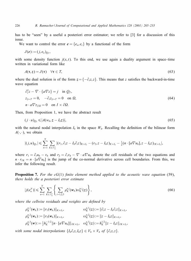
226 R. Rannacher / Journal of Computational and Applied Mathematics 128 (2001) 205–233
has to be “seen” by a useful a posteriori error estimator; we refer to [3] for a discussion of thisissue.
We want to control the error e = {eu; ev} by a functional of the form
J (e) := (j; eu)QT ;
with some density function j(x; t). To this end, we use again a duality argument in space–timewritten in variational form like
A(�; z) = J (�) ∀� ∈ T; (63)
where the dual solution is of the form z={−@tz; z}. This means that z satis$es the backward-in-timewave equation
@2t z −� · {a�z}= j in QT ;
z|t=T = 0; −@tz|t=T = 0 on �;
n · a�z|@� = 0 on I × @�:
(64)
Then, from Proposition 1, we have the abstract result
(j · u)QT6|A(wh; z − Ihz)|; (65)
with the natural nodal interpolation Ih in the space Wh. Recalling the de$nition of the bilinear formA(·; ·), we obtain
|(j; u)QT |6N∑
n=1
∑K∈Tn
h
|(r1; @tz − Ih@tz)K×In − (r2; z − Ihz)K×In − 12 (n · [a�uh]; z − Ihz)@K×In |;
where r1 = @tuh − vh and r2 = @tvh − � · a�uh denote the cell residuals of the two equations andn · r@K = n · [a�uh] is the jump of the co-normal derivative across cell boundaries. From this, weinfer the following result.
Proposition 7. For the cG(1) 7nite element method applied to the acoustic wave equation (59),there holds the a posteriori error estimate
|j(eNu )|6N∑
n=1
∑K∈Tn
h
{ ∑i=1;2;3
�n; iK (wh)!
n; iK (z)
}; (66)
where the cellwise residuals and weights are de7ned by
�n;1K (wh) := ‖r1(wh)‖K×In ; !n;1
K (z) := ‖@tz − Ih@tz‖K×In ;
�n;2K (wh) := ‖r2(wh)‖K×In ; !n;2
K (z) := ‖z − Ihz‖K×In ;
�n;3K (w) := 1
2h−1=2K ‖n · [a�uh]‖@K×In ; !n;3
K (z) := h1=2K ‖z − Ihz‖@K×In ;
with some nodal interpolations {Ih@tz; Ihz} ∈ Vh × Vh of {@tz; z}.
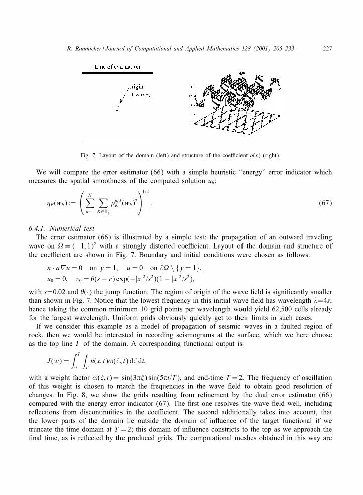
R. Rannacher / Journal of Computational and Applied Mathematics 128 (2001) 205–233 227
Fig. 7. Layout of the domain (left) and structure of the coe<cient a(x) (right).
We will compare the error estimator (66) with a simple heuristic “energy” error indicator whichmeasures the spatial smoothness of the computed solution uh:
�E(wh) :=
N∑
n=1
∑K∈Tn
h
�n;3K (wh)2
1=2
: (67)
6.4.1. Numerical testThe error estimator (66) is illustrated by a simple test: the propagation of an outward traveling
wave on � = (−1; 1)2 with a strongly distorted coe<cient. Layout of the domain and structure ofthe coe<cient are shown in Fig. 7. Boundary and initial conditions were chosen as follows:
n · a�u= 0 on y = 1; u= 0 on @� \ {y = 1};u0 = 0; v0 = A(s− r) exp(−|x|2=s2)(1− |x|2=s2);
with s=0:02 and A(·) the jump function. The region of origin of the wave $eld is signi$cantly smallerthan shown in Fig. 7. Notice that the lowest frequency in this initial wave $eld has wavelength '=4s;hence taking the common minimum 10 grid points per wavelength would yield 62,500 cells alreadyfor the largest wavelength. Uniform grids obviously quickly get to their limits in such cases.
If we consider this example as a model of propagation of seismic waves in a faulted region ofrock, then we would be interested in recording seismograms at the surface, which we here chooseas the top line 1 of the domain. A corresponding functional output is
J (w) =∫ T
0
∫1u(x; t)!(B; t) dB dt;
with a weight factor !(B; t)= sin(3�B) sin(5�t=T ), and end-time T =2. The frequency of oscillationof this weight is chosen to match the frequencies in the wave $eld to obtain good resolution ofchanges. In Fig. 8, we show the grids resulting from re$nement by the dual error estimator (66)compared with the energy error indicator (67). The $rst one resolves the wave $eld well, includingre=ections from discontinuities in the coe<cient. The second additionally takes into account, thatthe lower parts of the domain lie outside the domain of in=uence of the target functional if wetruncate the time domain at T =2; this domain of in=uence constricts to the top as we approach the$nal time, as is re=ected by the produced grids. The computational meshes obtained in this way are

228 R. Rannacher / Journal of Computational and Applied Mathematics 128 (2001) 205–233
Fig. 8. Grids produced from re$nement by the energy error indicator (67) (top row) and by the dual estimator (66)(bottom row) at times t = 0; 23 ;
43 ; 2.
obviously much more economical, without degrading the accuracy-in approximating the quantity ofinterest; for more examples see [3].
6.5. An optimal control model problem
As the last application of the general framework laid out in Section 2, we consider the $niteelement approximation of an optimal control problem. The state equations are
−Vu+ u= f on �;
@nu= q on 1C; @nu= 0 on @� \ 1C; (68)
de$ned on a bounded domain �⊂R2 with boundary @�. The control q acts on the boundarycomponent 1C, while the observations u|1O are taken on a component 1O; see Fig. 9. The costfunctional is de$ned by
J (u; q) = 12‖u− uO‖21O
+ 12D‖q‖21C
: (69)
with a prescribed function uO and a regularization parameter D¿ 0.We want to apply the general formalism of Section 2 to the Galerkin $nite element approximation
of this problem. This may be considered within the context of “model reduction” in optimal controltheory. First, we have to prepare the corresponding functional analytic setting. The functional ofinterest is the Lagrangian functional of the optimal control problem,
L(C) = J (u; q) + (�u;�') + (u− f; ')− (q; ')1C ;
de$ned for triples C = {u; '; q} in the Hilbert space W :=V × V × Q, where V :=H 1(�) andQ :=L2(1C). The equation for stationary points C = {u; '; q} ∈ W of L(·) are (Euler–Lagrangeequations)
L′(C;’) = 0 ∀’ ∈ W; (70)
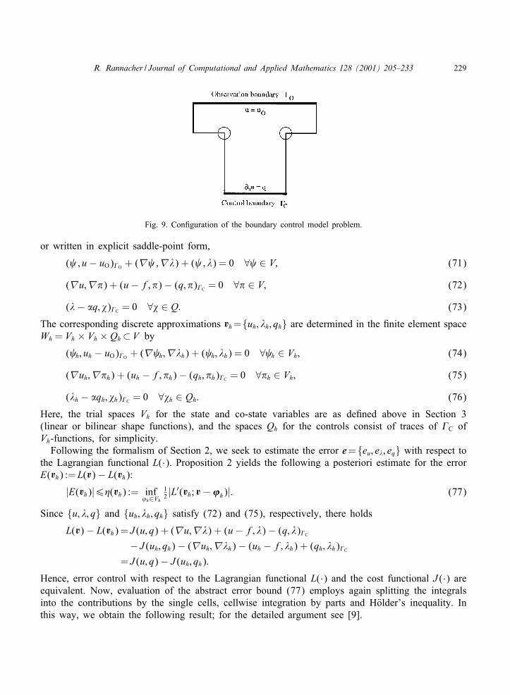
R. Rannacher / Journal of Computational and Applied Mathematics 128 (2001) 205–233 229
Fig. 9. Con$guration of the boundary control model problem.
or written in explicit saddle-point form,
( ; u− uO)1O + (� ;�') + ( ; ') = 0 ∀ ∈ V; (71)
(�u;�E) + (u− f; E)− (q; E)1C = 0 ∀E ∈ V; (72)
('− Dq; F)1C = 0 ∀F ∈ Q: (73)
The corresponding discrete approximations Ch={uh; 'h; qh} are determined in the $nite element spaceWh = Vh × Vh × Qh⊂V by
( h; uh − uO)1O + (� h;�'h) + ( h; 'h) = 0 ∀ h ∈ Vh; (74)
(�uh;�Eh) + (uh − f; Eh)− (qh; Eh)1C = 0 ∀Eh ∈ Vh; (75)
('h − Dqh; Fh)1C = 0 ∀Fh ∈ Qh: (76)
Here, the trial spaces Vh for the state and co-state variables are as de$ned above in Section 3(linear or bilinear shape functions), and the spaces Qh for the controls consist of traces of 1C ofVh-functions, for simplicity.
Following the formalism of Section 2, we seek to estimate the error e={eu; e'; eq} with respect tothe Lagrangian functional L(·). Proposition 2 yields the following a posteriori estimate for the errorE(Ch) :=L(C)− L(Ch):
|E(Ch)|6�(Ch) := inf’h∈Vh
12 |L′(Ch; C− ’h)|: (77)
Since {u; '; q} and {uh; 'h; qh} satisfy (72) and (75), respectively, there holds
L(C)− L(Ch) = J (u; q) + (�u;�') + (u− f; ')− (q; ')1C
− J (uh; qh)− (�uh;�'h)− (uh − f; 'h) + (qh; 'h)1C
= J (u; q)− J (uh; qh):
Hence, error control with respect to the Lagrangian functional L(·) and the cost functional J (·) areequivalent. Now, evaluation of the abstract error bound (77) employs again splitting the integralsinto the contributions by the single cells, cellwise integration by parts and HKolder’s inequality. Inthis way, we obtain the following result; for the detailed argument see [9].
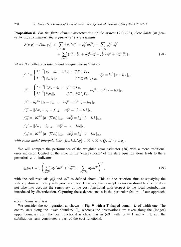
230 R. Rannacher / Journal of Computational and Applied Mathematics 128 (2001) 205–233
Proposition 8. For the 7nite element discretization of the system (71)–(73), there holds (in 7rst-order approximation) the a posteriori error estimate
|J (u; q)− J (uh; qh)|6∑
1⊂ @�
{�(')1 !(u)
1 + �(u)1 !(')
1 }+∑
1⊂1C
�(q)1 !(q)
1
+∑K∈Th
{�(u)K !(')
K + �(u)@K!
(')@K + �(')
K !(u)K + �(')
@K!(u)@K}; (78)
where the cellwise residuals and weights are de7ned by
�(')1 =
h−1=21 ‖uh − uO + @n'h‖1 if1⊂1O;
h−1=21 ‖@n; 'h‖1 if1⊂ @� \ 1O;
!(u)1 = h1=21 ‖u− Ihu‖1;
�(u)1 =
h−1=21 ‖@nuh − qh‖1 if1⊂1C;
h−1=21 ‖@nuh‖1 if1⊂ @� \ 1C;
!(')1 = h1=21 ‖'− Ih'‖1;
�(q)1 = h−1=2
1 ‖'h − Dqh‖1; !(q)1 = h1=21 ‖q− Ihq‖1;
�(u)K = ‖Vuh − uh + f‖K ; !(')
K = ‖'− Ih'‖K ;�(u)@K = 1
2h−1=2K ‖n · [�uh]‖@K ; !(')
@K = h1=2K ‖'− Ih'‖@K ;
�(')K = ‖V'h − 'h‖K ; !(u)
K = ‖u− Ihu‖K ;�(')@K = 1
2h−1=2K ‖n · [�'h]‖@K ; !(u)
@K = h1=2K ‖u− Ihu‖@K ;with some nodal interpolations {Ihu; Ih'; Ihq} ∈ Vh × Vh × Qh of {u; '; q}.
We will compare the performance of the weighted error estimator (78) with a more traditionalerror indicator. Control of the error in the “energy norm” of the state equation alone leads to the aposteriori error indicator
�E(uh) := cI
( ∑K∈Th
h2K{�(u)2K + �(u)2
@K }+∑
1⊂ @�
h21�(u)21
)1=2; (79)
with the cell residuals �(u)@K and �(u)
1 as de$ned above. This ad-hoc criterion aims at satisfying thestate equation uniformly with good accuracy. However, this concept seems questionable since it doesnot take into account the sensitivity of the cost functional with respect to the local perturbationsintroduced by discretization. Capturing these dependencies is the particular feature of our approach.
6.5.1. Numerical testWe consider the con$guration as shown in Fig. 9 with a T-shaped domain � of width one. The
control acts along the lower boundary 1C, whereas the observations are taken along the (longer)upper boundary 1O. The cost functional is chosen as in (69) with uO ≡ 1 and D = 1, i.e., thestabilization term constitutes a part of the cost functional.
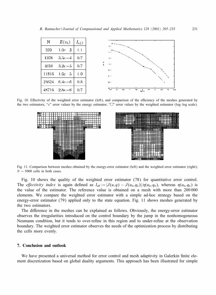
R. Rannacher / Journal of Computational and Applied Mathematics 128 (2001) 205–233 231
Fig. 10. E%ectivity of the weighted error estimator (left), and comparison of the e<ciency of the meshes generated bythe two estimators, “x” error values by the energy estimator, “ ” error values by the weighted estimator (log–log scale).
Fig. 11. Comparison between meshes obtained by the energy-error estimator (left) and the weighted error estimator (right);N ∼ 5000 cells in both cases.
Fig. 10 shows the quality of the weighted error estimator (78) for quantitative error control.The e>ectivity index is again de$ned as Ie% := |J (u; q) − J (uh; qh)|=�(uh; qh), whereas �(uh; qh) isthe value of the estimator. The reference value is obtained on a mesh with more than 200 000elements. We compare the weighted error estimator with a simple ad-hoc strategy based on theenergy-error estimator (79) applied only to the state equation. Fig. 11 shows meshes generated bythe two estimators.
The di%erence in the meshes can be explained as follows. Obviously, the energy-error estimatorobserves the irregularities introduced on the control boundary by the jump in the nonhomogeneousNeumann condition, but it tends to over-re$ne in this region and to under-re$ne at the observationboundary. The weighted error estimator observes the needs of the optimization process by distributingthe cells more evenly.
7. Conclusion and outlook
We have presented a universal method for error control and mesh adaptivity in Galerkin $nite ele-ment discretization based on global duality arguments. This approach has been illustrated for simple

232 R. Rannacher / Journal of Computational and Applied Mathematics 128 (2001) 205–233
examples of linear and nonlinear di%erential equations including also an optimal control problem.More challanging applications involving multi-physical e%ects like, for example, low-Mach number=ows with chemical reactions and multidimensional energy transfer by radiation with recombinationare presently studied. Of course, despite the generality of the method, there are several technicalquestions to be addressed in the future. The main problem is the accurate but cost-e<cient deter-mination of the dual solution especially in the presence of oscillatory solutions (wave propagation).Another question is the reliable control of the linearization in the neighborhood of a bifurcationpoint. Finally, the cost-e<cient application of our method for truly nonstationary problems in twoand particularly in three dimensions is still a largely unsolved problem.
Acknowledgements
The author acknowledges the support by the German Research Association (DFG) through theSFB 359 “Reactive Flow, Di%usion and Transport”, University of Heidelberg.
References
[1] M. Ainsworth, J.T. Oden, A posteriori error estimation in $nite element analysis, Comput. Methods Appl. Mech.Eng. 142 (1997) 1–88.
[2] W. Bangerth, Adaptive Finite-Elemente-Methoden zur LKosung der Wellengleichung mit Anwendungen in der Physikder Sonne, Diploma Thesis, Institut fKur Angewandte Mathematik, UniversitKat Heidelberg, 1998.
[3] W. Bangerth, R. Rannacher, Finite element approximation of the acoustic wave equation: error control and meshadaptation, East–West J. Numer. Math. 7 (1999) 263–282.
[4] R. Becker, An adaptive $nite element method for the incompressible Navier–Stokes equations on time-dependentdomains, Doctor Thesis, preprint 95-44, SFB 359, UniversitKat Heidelberg, 1995.
[5] R. Becker, Weighted error estimators for $nite element approximations of the incompressible Navier–Stokesequations, Technical Report 98-20, SFB 359, UniversitKat Heidelberg, 1998.
[6] R. Becker, M. Braack, R. Rannacher, Numerical simulation of laminar =ames at low Mach number with adaptive$nite elements, Combust. Theory Modelling 3 (1999) 503–534.
[7] R. Becker, M. Braack, R. Rannacher, C. Waguet, Fast and reliable solution of the Navier–Stokes equations includingchemistry, Comput. Visualization Sci. 2 (1999) 107–122.
[8] R. Becker, C. Johnson, R. Rannacher, Adaptive error control for multigrid $nite element methods, Computing 55(1995) 271–288.
[9] R. Becker, H. Kapp, R. Rannacher, Adaptive $nite element methods for optimal control of partial di%erentialequations: basic concepts, preprint 98-55, SFB 359, UniversitKat Heidelberg, 1998, SIAM J. Control Optim., toappear.
[10] R. Becker, R. Rannacher, Weighted a posteriori error control in FE methods, lecture at ENUMATH 95, Paris, August1995, in: H.G. Bock et al. (Eds.), Proceedings of ENUMATH 97, World Scient. Publ., Singapore, 1998.
[11] R. Becker, R. Rannacher, A feed-back approach to error control in $nite element methods: basic analysis andexamples, East–West J. Numer. Math. 4 (1996) 237–264.
[12] K. Eriksson, D. Estep, P. Hansbo, C. Johnson, Introduction to adaptive methods for di%erential equations,in: A. Iserles (Ed.), Acta Numerica 1995, Cambridge University Press, Cambridge, 1995, pp. 105–158.
[13] R. Hartmann, A posteriori FehlerschKatzung und adaptive Schrittweiten- und Ortsgittersteuerung beiGalerkin-Verfahren fKur die WKarmeleitungsgleichung, Diploma Thesis, Institut fKur Angewandte Mathematik,UniversitKat Heidelberg, 1998.
[14] P. Houston, R. Rannacher, E. SKuli, A posteriori error analysis for stabilised $nite element approximation of transportproblems, Report No. 99=04, Oxford University Computing Laboratory, Oxford, 1999, Comput. Methods Appl. Mech.Eng., to appear.
R. Rannacher / Journal of Computational and Applied Mathematics 128 (2001) 205–233 233
[15] C. Johnson, Numerical Solution of Partial Di%erential Equations by the Finite Element Method, Cambridge UniversityPress, Cambridge-Lund, 1987.
[16] C. Johnson, A new paradigm for adaptive $nite element methods, in: J. Whiteman (Ed.), Proceedings of MAFELAP93, Wiley, New York, 1993.
[17] C. Johnson, P. Hansbo, Adaptive $nite elemente methods in computational mechanics, Comput. Meth. Appl. Mech.Eng. 101 (1992) 143–181.
[18] G. Kanschat, E<cient and reliable solution of multi-dimensional radiative transfer problems, Proceedings ofMultiscale Phenomena and Their Simulation, World Scient. Publ., Singapore, 1997.
[19] R. Rannacher, Error control in $nite element computations, in: H. Bulgak, C. Zenger (Eds.), Proceedings of SummerSchool Error Control and Adaptivity in Scienti$c Computing, Kluwer Academic Publishers, Dordrecht, 1998, pp.247–278.
[20] R. Rannacher, F.-T. Suttmeier, A posteriori error estimation and mesh adaptation for $nite element models inelasto-plasticity, Comput. Methods Appl. Mech. Eng. 176 (1999) 333–361.
[21] F.-T. Suttmeier, Adaptive $nite element approximation of problems in elasto-plasticity theory, Doctor Thesis, Preprint97-11, SFB 359, UniversitKat Heidelberg, 1997.
[22] R. VerfKurth, A Review of A Posteriori Error Estimation and Adaptive Mesh-Re$nement Techniques, Wiley=Teubner,New York, Stuttgart, 1996.
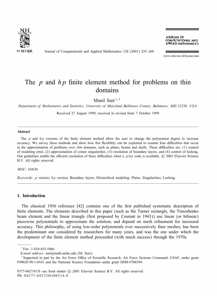
Journal of Computational and Applied Mathematics 128 (2001) 235–260www.elsevier.nl/locate/cam
The p and hp $nite element method for problems on thindomains
Manil Suri ∗; 1Department of Mathematics and Statistics, University of Maryland Baltimore County, Baltimore, MD 21250, USA
Received 27 August 1999; received in revised form 7 October 1999
Abstract
The p and hp versions of the $nite element method allow the user to change the polynomial degree to increaseaccuracy. We survey these methods and show how this /exibility can be exploited to counter four di1culties that occurin the approximation of problems over thin domains, such as plates, beams and shells. These di1culties are: (1) controlof modeling error, (2) approximation of corner singularities, (3) resolution of boundary layers, and (4) control of locking.Our guidelines enable the e1cient resolution of these di1culties when a p=hp code is available. c© 2001 Elsevier ScienceB.V. All rights reserved.
MSC: 65N30
Keywords: p version; hp version; Boundary layers; Hierarchical modeling; Plates; Singularities; Locking
1. Introduction
The classical 1956 reference [42] contains one of the $rst published systematic description of$nite elements. The elements described in this paper (such as the Turner rectangle, the Timoshenkobeam element and the linear triangle ($rst proposed by Courant in 1943)) use linear (or bilinear)piecewise polynomials to approximate the solution, and depend on mesh re$nement for increasedaccuracy. This philosophy, of using low-order polynomials over successively $ner meshes, has beenthe predominant one considered by researchers for many years, and was the one under which thedevelopment of the $nite element method proceeded (with much success) through the 1970s.
∗ Fax: 1-410-455-1066.E-mail address: [email protected] (M. Suri).1 Supported in part by the Air Force O1ce of Scienti$c Research. Air Force Systems Command, USAF, under grant
F49620-98-1-0161 and the National Science Foundation under grant DMS-9706594.
0377-0427/01/$ - see front matter c© 2001 Elsevier Science B.V. All rights reserved.PII: S 0377-0427(00)00514-8
236 M. Suri / Journal of Computational and Applied Mathematics 128 (2001) 235–260
Experiments by Szabo and his group conducted in the mid-1970s [41] indicated that an alternativestrategy might hold great promise as well. Their idea was to keep the mesh $xed, but increase thepolynomial degree for accuracy. They called this the p version, to distinguish it from the classicalmethod, which was labelled the h version. Computations on the elasticity problem indicated that thisnew philosophy was always competitive with, and often out-performed, the traditional h version.The $rst theoretical paper on the p version was published by BabuGska et al. in 1981 [11], andshowed, among other results, that the convergence rate was double that the h version for domainswith corners, and exponential for smooth solutions.
The collaboration between BabuGska and Szabo also led to the development of the so-called hpversion, which combines both strategies. It was shown that with proper mesh selection=re$nementcoupled with increase of polynomial degrees, an exponential convergence rate could be achievedeven for unsmooth solutions, i.e. in the presence of corner singularities. The $rst mathematical paperon the hp version was by BabuGska and Dorr, and appeared in 1981 [2].
Since the advent of these $rst results, the p and hp versions have, over the past two decades,come into their own as viable complements to the h version. Various commercial codes, such asSTRESS CHECK, POLYFEM, PHLEX, APPLIED STRUCTURE, MSC-NASTRAN (among others)have either been developed or modi$ed to include p=hp capability. While no single strategy (suchas h, p or hp re$nement) can be expected to be optimal for all problems, having both h and pcapability allows a level of /exibility that can often be exploited to signi$cantly increase accuracyand e1ciency. In particular, the high rates of convergence aKorded by p=hp techniques when corner(r�) singularities are present in the solution puts these methods ahead of traditional h-re$nement forsome important classes of problems.
In this paper, we bring out some of these advantages of p=hp methods. Rather than give a generalsurvey of such methods (for which the reader is referred, e.g., to [9], and to the books [40,31]), welist some important properties in Section 2, and then concentrate mainly on one class of problems— that of linear elasticity posed on thin domains such as beams, plates and shells. This class ofproblems is one that comes up very frequently in engineering structural analysis. In Sections 3–6, we discuss four areas where p=hp capability leads to advantages in approximation: (1) controlof modeling error, (2) good approximation of singularities occurring at the corners of the domain,(3) accurate resolution of boundary layers, and (4) control of locking phenomena. In the course ofour discussion, we also consider related problems where p=hp versions have advantages, such assingularly perturbed second order elliptic PDEs, which can result in stronger boundary layers thanthe ones found in plate models.
2. h; p and hp �nite element spaces
Suppose we are given a problem in variational form: Find u ∈ V such that
B(u; v) = F(v); v ∈ V: (2.1)
Here F is a bounded linear functional on the (in$nite dimensional) Hilbert space V , and B(· ; ·) isa bounded, coercive, symmetric, bilinear form on V ×V . Then given a sequence of ($nite element)subspaces {VN}⊂V , we can de$ne the $nite element approximations uN ∈ VN satisfying
B(uN ; v) = F(v); v ∈ VN : (2.2)
M. Suri / Journal of Computational and Applied Mathematics 128 (2001) 235–260 237
It is easily shown that
‖u− uN‖E6 infv∈VN
‖u− v‖E; (2.3)
where ‖ · ‖E is the energy norm
‖u‖E = (B(u; u))1=2: (2.4)
The coercivity and boundedness of B then gives
‖u− uN‖V6C infv∈VN
‖u− v‖V (2.5)
but, as we shall see, the constant C in (2.5) can be large for some problems.In all our examples, V will satisfy H 1
0 (�)⊂V ⊂H 1(�) 2 where �⊂Rt ; t = 1; 2; 3 is a boundeddomain with piecewise analytic boundary. The $nite element spaces VN will then consist of contin-uous piecewise polynomials de$ned on some mesh TN on �. We describe these in more detail forthe case �⊂R2.
Assume each TN is a regular [13] mesh consisting of straight-sided triangles and parallelograms{�Ni }; i=1; 2; : : : ; I(N ) (more general curvilinear elements could also be considered). For any elementS, we de$ne for p¿0 integer, Pp(S) (Qp(S)) to be the set of all polynomials of total degree (degreein each variable) 6p. We also denote Q′
p(S) = span{Pp(S); xpy; xyp}. Let pN be a degree vectorassociating degree pN
i to element �Ni (if pNi is independent of i, we write pN = pN ). Then the local
polynomial spaces are denoted RN (�Ni ) where RN = PpNi
if �Ni is a triangle and RN = QpNi
or Q′pN
i
if �Ni is a parallelogram. We then set
VN = {v ∈ V; v|� Ni∈ RN (�Ni )}
(VN ⊂C(0)(�) for our examples).Let us denote hN
i = diam(�Ni ); hN = maxi hNi ; hN = mini hN
i . The sequence {TN} is called quasi-uniform provided there exists � independent of N such that
hN
hN6�:
As we shall see, spaces on quasiuniform meshes do not have the best properties where approximationof corner singularities is concerned. Rather, such singularities must be treated by nonquasiuniformmesh re$nement, where the mesh becomes $ner as one approaches the point of singularity. Thetype of mesh used in the hp version is geometric, and is de$ned below for the case of re$nementtowards the origin O. (Fig. 1 gives a more intuitive idea than the de$nition, which is technical.)
Let 0¡q¡ 1 be a number called the geometric ratio. Let n(=nN ) be the number of layersaround the origin O. We denote the elements of TN by �Nn; j; k where j = 1; : : : ; �(k); �(k)6�0 andk = 1; 2; : : : ; n + 1. Let hn; j; k = diam(�Nn; j; k) and dn;j; k = dist(�Nn; j; k ;O). Then
(A) if O ∈ P�Nn; j; k , for j = 1; : : : ; �(k); k = 2; : : : ; n + 1,
C1qn+2−k6dn;j; k6C2qn+1−k ;
�1dn;j; k6hn; j; k6�2dn;j; k :
2 We use standard Sobolev space notation: Hk(!) is the space of functions with k derivatives that are square integrableover !. H 1
0 (!) is the subset of functions in H 1(!) with vanishing trace on @!. ‖ · ‖Hk (!) is the norm of Hk(!).

238 M. Suri / Journal of Computational and Applied Mathematics 128 (2001) 235–260
Fig. 1. Types of re$nement: (a) quasiuniform, (b) geometric.
(B) if O ∈ P�Nn; j; k , then k = 1 and for j = 1; : : : ; �(1),
�3qn6hn; j; k6�4qn:
The constants Ci and �i are independent of N . See [21], where it is empirically shown thatq ≈ 0:15 is the best choice in terms of approximability. (In one dimension, this is theoreticallyestablished in [20].)
We can now talk about the following extension procedures, i.e. strategies for increasing thedimension of the space VN to get a more accurate estimate in (2.3).
(i) h version: The most basic extension procedure consists of using quasiuniform meshes {TN} withsuccessively smaller hN , with uniform pN =p, kept $xed at p=1 or 2 usually. Nonquasiuniformmeshes (such as radical meshes, see [9]) could also be used.
(ii) p version: Here, TN is the same for all N . Accuracy is achieved by increasing pN . The meshcould be uniform, but if a properly re$ned mesh (Fig. 1(b)) is used, the p version can oftenbe made to yield the superior performance of the hp version (which is harder to implement).
(iii) hp version: Any {VN} for which both TN and pN are changed will give rise to an hp version.For instance, in Section 5, we consider an hp version designed to resolve boundary layers,where as pN is increased, the number of elements remains the same, but the size of elementschanges. For treating corner singularities, the geometric meshes with n layers described aboveare used, with pN chosen uniformly to be pN =�nN (� $xed), so that both pN and nN increasesimultaneously. Even more e1cient is the case that pN is chosen to be the same over allelements in layer k, i.e. over all �Nn; j; k for j = 1; : : : ; �(k), and increasing linearly with the indexk = 1; 2; : : : ; n + 1 (see [21] for more details).
Let us mention that there are several diKerences between implementation of p=hp methods andthe traditional h methods (for instance, the basis functions used in the p version are often not ofnodal type). We do not discuss these aspects here but instead refer the reader to [40].

M. Suri / Journal of Computational and Applied Mathematics 128 (2001) 235–260 239
To conclude this section, we present the following theorem, which gives the basic estimate for thein$mum in (2.5) when the norm ‖·‖V =‖·‖H 1(�) and when the h; p or hp version over quasiuniformmeshes is used.
Theorem 2.1 (BabuGska and Suri [7]). Let the spaces VN consist of piecewise polynomials of degreepN over a quasiuniform family of meshes {TN} on �⊂Rt ; t = 1; 2; 3. Then for u ∈ Hk(�); k¿1;
infv∈VN
‖u− v‖H 1(�)6Chmin(k−1;pN )N p−(k−1)
N ‖u‖Hk (�) (2.6)
with C a constant independent of u and N . (For a nonuniform distribution pN ; we replace pN bymin( pN ) in (2:6)).
Theorem 2.1 combined with (2.5) immediately shows that the following rates of convergencehold:
h version : ‖u− uN‖V = O(hmin(k−1;pN )N ); (2.7)
p version : ‖u− uN‖V = O(p−(k−1)N ): (2.8)
Since the number of degrees of freedom N ∼ O(h−tN pt
N ), we see that asymptotically, the rate ofconvergence (in terms of N ) of the p version is never lower than that of the h version. In fact, forsmooth solutions, it is often much better, as seen from (2.8) (“spectral” convergence). As we shallsee in Section 4, the rate can be better even when the solution is not smooth.
3. Control of modeling error
Structural analysis over a three-dimensional domain (thin or otherwise) involves solving the equa-tions of three-dimensional elasticity on the domain. When three-dimensional $nite elements are used,the number of degrees of freedom N grows quite rapidly. For instance, while N ∼ O(h−2) or O(p2)in two dimensions (for the h and p versions, respectively), we have N ∼ O(h−3) or O(p3) in threedimensions. In the case that one dimension of the domain is thin, the three-dimensional model isoften replaced by a two-dimensional model, formulated generally on the mid-plane of the domain.Discretization of this two-dimensional model then requires fewer degrees of freedom.
Let us present an illustrative example, that of a thin plate. Let ! be a bounded domain in R2
with piecewise smooth boundary, which represents the midplane of the plate, which we assume tobe of thickness d (d diam(!)). Then, we represent the three-dimensional plate as
� = {x = (x1; x2; x3) ∈ R3 | (x1; x2) ∈ !; |x3|¡d=2}:The lateral surface S and top and bottom surfaces R± are given by (see Fig. 2)
S = {x ∈ R3 | (x1; x2) ∈ @!; |x3|¡d=2};R± = {x ∈ R3 | (x1; x2) ∈ !; x3 =±d=2}:
Let us denote the displacement u = (u1; u2; u3). Then we consider the problem of $nding u ∈H 1
D(�) = {u ∈ (H 1(�))3 | u3 = 0 on S} which satis$es
B(u; C) = F(C) ∀C ∈ H 1D(�); (3.1)
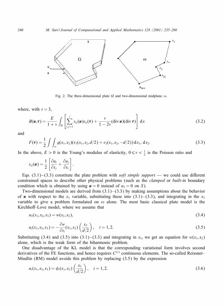
240 M. Suri / Journal of Computational and Applied Mathematics 128 (2001) 235–260
Fig. 2. The three-dimensional plate � and two-dimensional midplane !.
where, with t = 3,
B(u; C) =E
1 + %
∫�
t∑
i; j=1
&ij(u)&ij(C) +%
1− 2%(div u)(div C)
dx (3.2)
and
F(C) =12
∫ ∫!g(x1; x2)(v3(x1; x2; d=2) + v3(x1; x2;−d=2)) dx1; dx2: (3.3)
In the above, E¿ 0 is the Young’s modulus of elasticity, 06%¡ 12 is the Poisson ratio and
&ij(u) =12
[@ui
@xj+
@uj
@xi
]:
Eqs. (3.1)–(3.3) constitute the plate problem with soft simple support — we could use diKerentconstrained spaces to describe other physical problems (such as the clamped or built-in boundarycondition which is obtained by using u = 0 instead of u3 = 0 on S).
Two-dimensional models are derived from (3.1)–(3.3) by making assumptions about the behaviorof u with respect to the x3 variable, substituting these into (3.1)–(3.3), and integrating in the x3
variable to give a problem formulated on ! alone. The most basic classical plate model is theKirchhoK–Love model, where we assume that
u3(x1; x2; x3) = w(x1; x2); (3.4)
ui(x1; x2; x3) =−@w@xi
(x1; x2)(
x3
d=2
); i = 1; 2: (3.5)
Substituting (3.4) and (3.5) into (3.1)–(3.3) and integrating in x3, we get an equation for w(x1; x2)alone, which is the weak form of the biharmonic problem.
One disadvantage of the KL model is that the corresponding variational form involves secondderivatives of the FE functions, and hence requires C(1) continuous elements. The so-called Reissner–Mindlin (RM) model avoids this problem by replacing (3.5) by the expression
ui(x1; x2; x3) = *i(x1; x2)(
x3
d=2
); i = 1; 2: (3.6)
M. Suri / Journal of Computational and Applied Mathematics 128 (2001) 235–260 241
Hence, we now have two more unknowns (*1; *2) =�. This leads to the following variational form,after some modi$cation of the elastic constants (see [5]): Find U = (�; w) ∈ V = H 1(�)×H 1(�)×H 1
D(�) satisfying for all W = (�; -) ∈ V ,
B(U;W ) = a(�; �) + /�d−2(�w + �;�- + �) =∫ ∫
!g- dx1 dx2; (3.7)
where
a(�; �) = D∫ ∫
!
(1− %)
2∑i; j=1
&ij(�)&ij(�) + %(div �)(div �)
dx1 dx2 (3.8)
and where D = E=12(1− %2); � = E=2(1 + %) and / is the shear correction factor.It is seen from (3.7) that the RM model essentially enforces the KirchhoK constraint,
KU =�w + � = 0 (3.9)
in a penalized form (while the KL model enforces it exactly).The replacement of the three-dimensional elasticity problem by a two-dimensional model such
as RM leads to a modeling error between the actual three-dimensional solution and the solutionobtained e.g. by (3.4)–(3.6). This modeling error is unaKected by any subsequent discretization ofthe two-dimensional model. The only way to decrease it is to use a more accurate model. To derivesuch more accurate models, we expand u(x1; x2; x3) in terms of higher-order polynomials of x3.
More precisely, let n=(n1; n2; n3) by a triple of integers ¿0. We then make the ansatz (for i=1; 2)
u3(x1; x2; x3) =n3∑j=0
wj(x1; x2)Lj
(x3
d=2
); (3.10)
ui(x1; x2; x3) =ni∑
j=0
*ij(x1; x2)Lj
(x3
d=2
); (3.11)
which when substituted into the three-dimensional equations gives us the so-called n = (n1; n2; n3)model upon integration. (Here {Lj} are the Legendre polynomials.) It is possible to show that (undersome assumptions)
(1) For n1¿1; n2¿1; n3¿2, models n=(n1; n2; n3) converge, as d→ 0, to the same limiting solutionas that obtained when d→ 0 in the three-dimensional elasticity equations. (For n= (1; 1; 0), thisis true with modi$ed elastic constants.)
(2) For $xed d, as min(n1; n2; n3) → ∞, the solutions of the models converge to the exact three-dimensional solution.
There are various factors such as boundary conditions, boundary layers, corner singularities, etc.,which aKect the convergence of a given model as d → 0 [6]. For instance, in [17] it is shownthat the RM model may not lead to good approximations of the boundary layer, while higher-ordermodels signi$cantly improve the convergence as d→ 0.
Let us denote for n = (n1; n2; n3)nH 1
D(�) = {u = (u1; u2; u3) ∈ H 1D(�) satisfying (3:10) and (3:11)}:
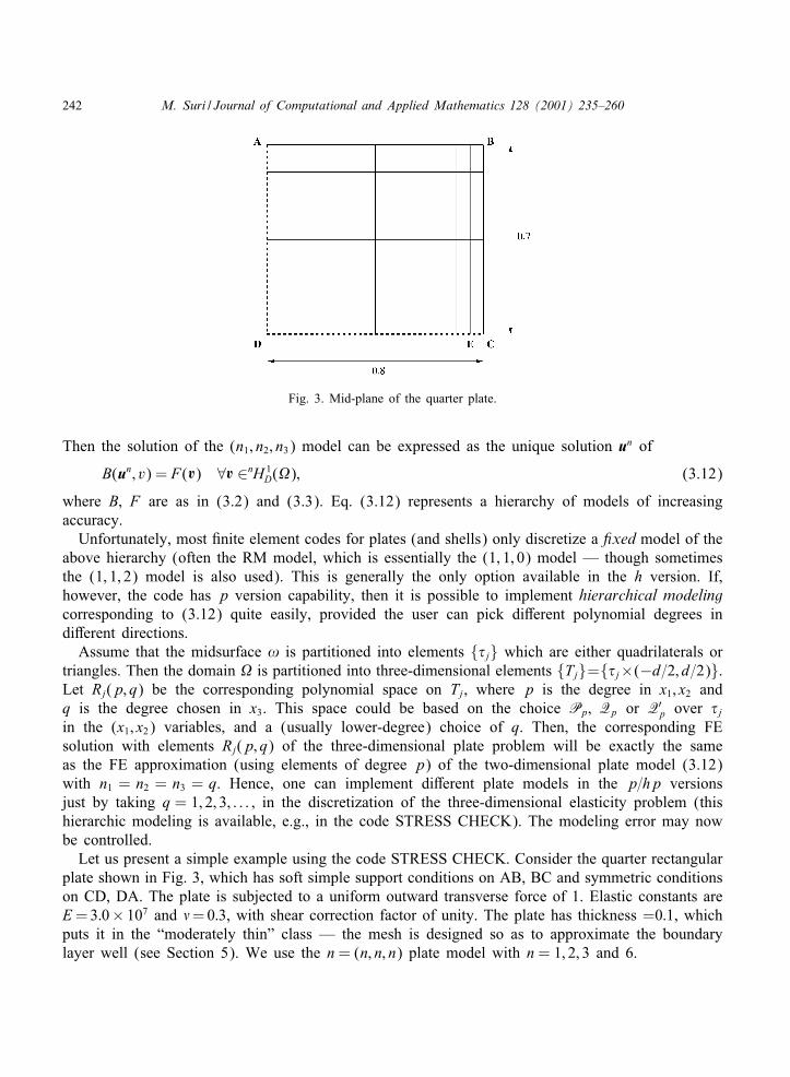
242 M. Suri / Journal of Computational and Applied Mathematics 128 (2001) 235–260
Fig. 3. Mid-plane of the quarter plate.
Then the solution of the (n1; n2; n3) model can be expressed as the unique solution un of
B(un; v) = F(C) ∀C ∈nH 1D(�); (3.12)
where B; F are as in (3.2) and (3.3). Eq. (3.12) represents a hierarchy of models of increasingaccuracy.
Unfortunately, most $nite element codes for plates (and shells) only discretize a 6xed model of theabove hierarchy (often the RM model, which is essentially the (1; 1; 0) model — though sometimesthe (1; 1; 2) model is also used). This is generally the only option available in the h version. If,however, the code has p version capability, then it is possible to implement hierarchical modelingcorresponding to (3.12) quite easily, provided the user can pick diKerent polynomial degrees indiKerent directions.
Assume that the midsurface ! is partitioned into elements {�j} which are either quadrilaterals ortriangles. Then the domain � is partitioned into three-dimensional elements {Tj}={�j×(−d=2; d=2)}.Let Rj(p; q) be the corresponding polynomial space on Tj, where p is the degree in x1; x2 andq is the degree chosen in x3. This space could be based on the choice Pp; Qp or Q′
p over �jin the (x1; x2) variables, and a (usually lower-degree) choice of q. Then, the corresponding FEsolution with elements Rj(p; q) of the three-dimensional plate problem will be exactly the sameas the FE approximation (using elements of degree p) of the two-dimensional plate model (3.12)with n1 = n2 = n3 = q. Hence, one can implement diKerent plate models in the p=hp versionsjust by taking q = 1; 2; 3; : : : ; in the discretization of the three-dimensional elasticity problem (thishierarchic modeling is available, e.g., in the code STRESS CHECK). The modeling error may nowbe controlled.
Let us present a simple example using the code STRESS CHECK. Consider the quarter rectangularplate shown in Fig. 3, which has soft simple support conditions on AB, BC and symmetric conditionson CD, DA. The plate is subjected to a uniform outward transverse force of 1. Elastic constants areE = 3:0× 107 and %= 0:3, with shear correction factor of unity. The plate has thickness =0:1, whichputs it in the “moderately thin” class — the mesh is designed so as to approximate the boundarylayer well (see Section 5). We use the n = (n; n; n) plate model with n = 1; 2; 3 and 6.

M. Suri / Journal of Computational and Applied Mathematics 128 (2001) 235–260 243
Fig. 4. Transverse displacement u3 along EC for diKerent models.
Fig. 5. Shear force distribution Qy along EC for diKerent models.
Figs. 4 and 5 show the extraction of two quantities — the transverse displacement u3 and theshear force Qy, along the lower edge of the element situated at the corner C. Degree p = 8 is usedfor the $nite element approximations. It is observed that while there is no appreciable diKerence foru3 with the model order, the quantity Qy does vary appreciably. The reason for this is that u3 hasa very weak boundary layer, while Qy has a stronger layer — and this is dependent on the modelorder (see [17] for more detailed experiments).
The above ideas also apply to other thin domains, such as composite plates and shells [10]. Forthese more complicated domains, the diKerences observed between diKerent model orders is usuallyeven more striking.
244 M. Suri / Journal of Computational and Applied Mathematics 128 (2001) 235–260
4. Approximation of singularities
The previous section showed how the three-dimensional elasticity equations over the plate � couldbe reduced to a hierarchy of elliptic problems (such as (3.7)) over the two-dimensional domain !(Fig. 2(b)). It is well known that linear elliptic problems will (in general) have singularities at thecorners Aj; j = 1; : : : ; M of the domain !, and also at points on @! where the type of boundarycondition changes, e.g., from Dirichlet to Neumann. For the three-dimensional problem over �, thesingularities will occur not only at vertices of � but also along its edges. One of the main advantagesof p=hp methods is that with proper mesh design, such singularities can be approximated very well.
4.1. A decomposition result
An examination of Eq. (3.7) shows that plate models such as the RM model are singularlyperturbed in the variable �. This results in boundary layers when d is small. The interaction ofcorner singularities and boundary layers is a complicated phenomenon, for which decomposition andregularity results may be found, e.g., in [25,16]. We will postpone the consideration of boundarylayer approximation to Section 5. Here, to simplify the exposition, we assume that the thickness dis a $xed positive constant and do not worry about our approximation results being uniform in d.
Accordingly, given a linear elliptic problem on ! (which is one of our (n1; n2; n3) models), wemay use the results of Kondratiev (see [26] and also [19,15]) to decompose the solution in theneighborhood of any vertex Aj. If U is the solution and (r; 6) are the polar coordinates with originat Aj, then we may write
U =L∑
‘=1
S∑s=0
T∑t=0
c‘st ‘st(6)r�‘+t lns r + U0
=L∑
‘=1
U‘ + U0 (4.1)
in the neighborhood of Aj. Here ‘st is a vector with the same number of components as U , andis analytic in 6. The exponents �‘ can be complex, and the coe1cients c‘st will depend on d. Bytaking L, S, T large enough, we can make U0 as smooth as the data will allow. In fact, taking thecorrect number of terms near each Aj, we may write
U =M∑j=1
∑‘
U ( j)‘ ;j + U0; (4.2)
where ;j is a smooth cut-oK function in the neighborhood of Aj and U0 satis$es the appropriateshift theorem (e.g., in the case of (3.7), we would have
‖U0‖[Hk+2(!)]36C(d)‖g‖Hk (!);
i.e., the same theorem as for a smooth boundary). Eqs. (4.1) and (4.2) show that when the $niteelement method is used, the rate of best approximation (i.e., the right side of (2.3)) will be deter-mined by the worst singularity min‘; j|�( j)
‘ | (and the corresponding S in decomposition (4.1)), sincethe other terms (including U0) are all smoother and hence result in better approximation rates.
M. Suri / Journal of Computational and Applied Mathematics 128 (2001) 235–260 245
4.2. hp convergence: quasiuniform meshes
We now present a theorem for the approximation of one of the canonical singularities present in(4.2), which we write as
u = r� lns r (6); (4.3)
where is a vector and for � complex, we understand r� to denote Re r�.First, we note that for !⊂R2, u ∈ H 1+�−&(!) for any &¿ 0, where � = Re �. We could apply
Theorem 2.1 to get an approximation rate of O(hmin(�−&;pN )N p−�+&
N ), but as shown in [7], this resultcan be improved to give the following theorem.
Theorem 4.1. Let u be given by (4:3). Let quasiuniform meshes be used. Then
infv∈VN
‖u− v‖H 1(!)6Ck(hN ; pN ; s) min
{h�N ;
hmin(�;pN−�)
p2�N
}; (4.4)
where k(hN ; pN ; s) = max(|lns hN |; |lns pN |) and C is a constant independent of N .
Theorem 4.1 shows that one gets the following convergence rates:
h version : O(h�N ); (4.5)
p version : O(p−2�N ): (4.6)
Since N = O(h−2N p2
N ), we see that the p version gives twice the convergence rate of the h version.This happens whenever the point of singularity r = 0 coincides with the node of an element. If thesingularity point lies in the interior of an element, then the doubling eKect does not take place.
Applying Theorem 4.1 to each component of (4.2) and assuming that U0 is smooth enough to bebetter approximated, we see that (4.4)–(4.6) will also hold for the error ‖U − UN‖V where UN isthe FEM approximation to U .
4.3. hp convergence: nonquasiuniform meshes
For the h version with polynomials of $xed degree p, it is well known that the optimal convergencerate for smooth functions is O(hp
N ). Hence, the rate (4.5) can be quite far from optimal if � is small(for example, �¡ 1 in nonconvex domains for the Poisson equation). It turns out that the useof nonquasiuniform meshes, which are increasingly re$ned towards the points of singularity, canincrease the convergence rate. The optimal meshes in this regard are the so-called radical meshes,which result in O(hp
N ) convergence for function (4.3) when the mesh is designed taking into accountthe strength of the singularity � and the degree of the polynomial p. We refer to [20] where a fullanalysis of such meshes is given in one dimension and to [4] where the case p = 1 is analyzed intwo dimensions.
Here, we present a result for the hp version, which shows that with the geometric meshes describedin Section 2, one obtains exponential convergence in terms of N , the number of degrees of freedom(note that O(hp
N ) convergence is only algebraic in N ). The spaces VN are chosen as follows. In thevicinity of each singularity point, a geometric mesh with nN layers (see Section 2) is constructed,
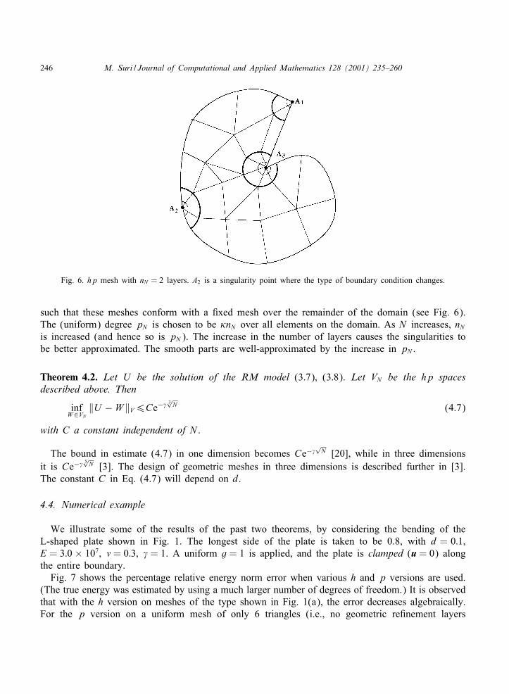
246 M. Suri / Journal of Computational and Applied Mathematics 128 (2001) 235–260
Fig. 6. hp mesh with nN = 2 layers. A2 is a singularity point where the type of boundary condition changes.
such that these meshes conform with a $xed mesh over the remainder of the domain (see Fig. 6).The (uniform) degree pN is chosen to be �nN over all elements on the domain. As N increases, nN
is increased (and hence so is pN ). The increase in the number of layers causes the singularities tobe better approximated. The smooth parts are well-approximated by the increase in pN .
Theorem 4.2. Let U be the solution of the RM model (3:7); (3:8). Let VN be the hp spacesdescribed above. Then
infW∈VN
‖U −W‖V6Ce−/ 3√N (4.7)
with C a constant independent of N .
The bound in estimate (4.7) in one dimension becomes Ce−/√
N [20], while in three dimensionsit is Ce−/ 5√N [3]. The design of geometric meshes in three dimensions is described further in [3].The constant C in Eq. (4.7) will depend on d.
4.4. Numerical example
We illustrate some of the results of the past two theorems, by considering the bending of theL-shaped plate shown in Fig. 1. The longest side of the plate is taken to be 0.8, with d = 0:1,E = 3:0 × 107; % = 0:3; / = 1. A uniform g = 1 is applied, and the plate is clamped (u = 0) alongthe entire boundary.
Fig. 7 shows the percentage relative energy norm error when various h and p versions are used.(The true energy was estimated by using a much larger number of degrees of freedom.) It is observedthat with the h version on meshes of the type shown in Fig. 1(a), the error decreases algebraically.For the p version on a uniform mesh of only 6 triangles (i.e., no geometric re$nement layers

M. Suri / Journal of Computational and Applied Mathematics 128 (2001) 235–260 247
Fig. 7. Error curves for h and p versions.
in Fig. 1(b)), the error follows an ‘S’ curve, with the middle portion representing an exponentialdecrease, and the /at portion representing twice the algebraic h version rate. When one layer of meshre$nement is introduced (as in the top of Fig. 1(b)), it is observed the exponential rate continuesthrough p = 8. Further mesh re$nement would only be useful when this graph /attens out as well— essentially, in the range of parameters shown, the p version is displaying the same exponentialrate of convergence expected from the hp version. For more detailed experiments, we refer, e.g.,to [7].
5. Resolution of boundary layers
If one lets d→ 0 in Eqs. (3.1)–(3.3), then one gets a system of singularly perturbed equations[16]. This will also be true for the (n1; n2; n3) model given by (3.12). For instance, it is clear from(3.7) and (3.8) that the RM model is singularly perturbed in � (but not in w), since multiplying(3.7) through by d2, the order of derivatives in � decreases to 0 as d → 0. This implies that formost boundary conditions � will have a boundary layer at @! for small d, i.e., components in thesolution of the form (Fig. 8)
�b(s; t) = C(d) f (t)e−ks=d: (5.1)
Here (s; t) are local coordinates in the normal and tangential directions at @!, k is a constant andf is a smooth function. The amplitude C(d) of the boundary layer will depend upon the type ofboundary conditions — for instance, the largest amplitude C(d) = O(d) occurs for the case of thesoft simple support and free plates, while for clamped (built-in) conditions, it is only O(d2) [1].

248 M. Suri / Journal of Computational and Applied Mathematics 128 (2001) 235–260
Fig. 8. The boundary layer.
The amplitude will have the same order (though not the same value [17]) for all (n1; n2; n3) platemodels. The only model free of boundary layers is the KL model. For a discussion of the relationof boundary layers in the three-dimensional case to those in (n1; n2; n3) models, we refer to [17].
Our concern in this section is the approximation of components such as (5.1) by the FEM. Wenote that the boundary layer eKect is essentially a one-dimensional eKect, so that if we can e1cientlyapproximate the functions �b in the normal direction, then we can expect to have an overall goodapproximation. Our $rst step, therefore, is to consider the approximation of the one-dimensionalboundary layer function
ud(x) = e−x=d (5.2)
by the space VN of piecewise polynomials of degree pN = (pN1 ; p
N2 ; : : : ; p
NI ) on the mesh TN = {0 =
x0 ¡x1; : : : ;¡ xI = 1}.Let us consider the approximation of (5.2) in the context of the one-dimensional singularly per-
turbed problem
− d2u′′d(x) + ud(x) = f(x); x ∈ I = (−1; 1); (5.3)
ud(±1) = �±: (5.4)
It is well known (see, e.g., [33]) that the solution of (5.3) and (5.4) can be decomposed as
ud(x) = usd + Adud(1 + x) + Bdud(1− x); (5.5)
i.e., it contains terms of form (5.2), plus a smooth (in d) component usd. Writing (5.3) and (5.4) in
variational form, we have that ud ∈ H 10 (I) satis$es ∀v ∈ H 1
0 (I),
Bd(ud; v) :=∫I{d2u′dv
′ + udv} dx =∫Ifv dx: (5.6)
We consider the approximation of Pud in the energy norm for (5.6), i.e., in the norm
‖v‖d = (Bd(v; v))1=2 ≈ d‖v′‖L2(I) + ‖v‖L2(I):

M. Suri / Journal of Computational and Applied Mathematics 128 (2001) 235–260 249
For the h version on a quasiuniform mesh, we may apply (2.6), together with an L2 duality result,to obtain (for k¿pN + 1)
infv∈VN
‖ud − v‖d6Chk−1N d−k+3=2; (5.7)
where we have used (5.2) to estimate ‖ Pud‖Hk (I). We see that for $xed d, we get the optimal O(hk−1N ),
but as d→ 0, this rate deteriorates. The best possible uniform rate for 0¡d61 is O(h1=2N ), obtained
by taking k = 32 . This is the rate observed in practice for d small.
For the p version, it is shown in [33] that the following theorem holds. Here, p :=p + 12 .
Theorem 5.1. (A) Let r = (e=2pNd)¡ 1. Then
infv∈VN
‖ud − v‖d6Cd1=2rpN (1− r2)−1=2; (5.8)
where C is a constant independent of pN and d.(B) We have
infv∈VN
‖ud − v‖d6Cp−1N
√ln pN ; (5.9)
uniformly for 0¡d61.
Theorem 5.1 shows that while rate (5.8) is exponential, it only holds for pN very large (notgenerally seen in practice). The best uniform rate is given by (5.9), and is twice that for the hversion (modulo the log factor).
Estimates (5.7) and (5.9) show that both the h and p versions give disappointing convergencerates uniform in d. One remedy for this is to use nonquasiuniform meshes, by which the O(hk−1
N )rate of the h version can be recovered. One such mesh is given in [33], by TN ={−1; x1; : : : ; xm−1; 1},where, for m even, and pN ≡ p,
xm=2±i =∓dp ln(1− 2ic=m); i = 0; : : : ; m=2 (5.10)
with c = 1− exp(1− 1=(dp)). See, e.g., [35,43] for other examples.Another solution, possible when both h and p capability is available, is to insert a single element
of size O(pd) at the boundary layer, and let p → ∞. This gives exponential convergence. Moreprecisely, the following theorem is established in [33].
Theorem 5.2. Let (TN ; pN ) be such that for p¿1;
pN = {p; 1}; TN = {−1;−1 + �pd; 1} if �pd¡ 2;
pN = {p}; TN = {−1; 1} if �pd¿2; (5.11)
where 0¡�06�¡ 4=e is a constant independent of p and d. Then with Pud = Pud(x + 1); thereexists 0¡�¡ 1 such that
infv∈VN
‖ud − v‖d6Cd1=2�p
with C; � independent of p and d.
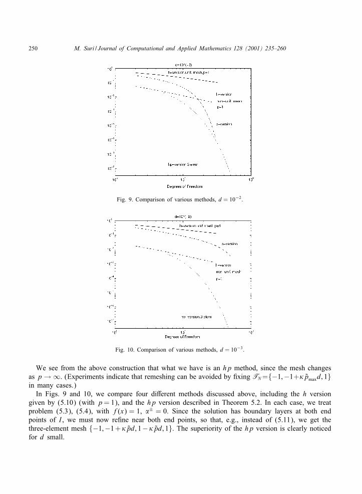
250 M. Suri / Journal of Computational and Applied Mathematics 128 (2001) 235–260
Fig. 9. Comparison of various methods, d = 10−2.
Fig. 10. Comparison of various methods, d = 10−3.
We see from the above construction that what we have is an hp method, since the mesh changesas p→∞. (Experiments indicate that remeshing can be avoided by $xing TN ={−1;−1+�pmaxd; 1}in many cases.)
In Figs. 9 and 10, we compare four diKerent methods discussed above, including the h versiongiven by (5.10) (with p = 1), and the hp version described in Theorem 5.2. In each case, we treatproblem (5.3), (5.4), with f(x) = 1, �± = 0. Since the solution has boundary layers at both endpoints of I , we must now re$ne near both end points, so that, e.g., instead of (5.11), we get thethree-element mesh {−1;−1 +�pd; 1−�pd; 1}. The superiority of the hp version is clearly noticedfor d small.

M. Suri / Journal of Computational and Applied Mathematics 128 (2001) 235–260 251
Fig. 11. Boundary-$tted mesh.
The above eKect may also be observed for two-dimensional problems. Consider the singularlyperturbed problem
− d2 Xu + u = f in !; (5.12)
u = 0 on @!: (5.13)
If ! is a smooth domain, then the solution will again have a component of the form (5.1), withC(d) = O(1). If we now construct a mesh in boundary-$tted coordinates (s; t), such that the (tensorproduct) basis functions are polynomials in s multiplied by polynomials in t, then the problem ofapproximating (5.1) reduces once more to a one-dimensional approximation. Hence, for example,we should take the mesh to be such that in the s direction, the $rst layer of elements is of O(�pd)(see Fig. 11). Then one can again establish exponential hp convergence for the solution of (5.12)and (5.13) uniform in d [44,45,27]. This may also be done when the meshes and basis functionsare suitably $tted in (x; y) rather than (s; t) coordinates, as long as the O(�pd) layer character ismaintained.
In Figs. 13 and 14, we show experiments performed using STRESS CHECK for (5.12) and (5.13)on the unit circle, with f = 1, for which the exact solution can be expressed in terms of a modi$edBessel function (Eq. (7:2) of [45]) and has a boundary layer at @!. We take pmax = 8 and performthe p version on the two meshes shown in Fig. 12. The $rst approximates the one from Theorem5.2, with a layer of elements of size pmaxd, while the second is a more uniform mesh, $xed for alld. The advantage of the $rst mesh is clearly demonstrated in Figs. 13 and 14.
The case of a nonsmooth domain is more subtle. For instance, if ! is a polygon, then thesingularities for (5.12) and (5.13) now behave essentially like (r=d)� [24]. Consequently, the meshre$nement for the singularities must now be carried out in an O(d) region of the corners, as shownin Fig. 15. In [47], spectral convergence of O(p−k), k arbitrary, has been established for suchmeshes as p→∞.
For the case of the RM plate, as noted before, the strongest boundary layer (in the case of the freeor the soft simply supported plate) is only O(d). Consequently, the re$nement of the singularities(i.e., usual O(1) hp re$nement) is usually su1cient in practice when the error in the energy normis of interest. However, if quantities involving the s-derivative of (5.1) are calculated (such as

252 M. Suri / Journal of Computational and Applied Mathematics 128 (2001) 235–260
Fig. 12. The two meshes.
Fig. 13. Comparison of p version, d = 10−2.
moments), then these will again contain an O(1) boundary layer, and re$nements such as that inFig. 15 will again be necessary (recall the example in Fig. 3, see, e.g., [34,46]).
For shell problems, the solutions have a rich array of boundary layers, which are often strongerthan those encountered in plates. Ideas similar to the ones discussed above may be applied to suchproblems as well. We refer to [23,29,18,22] for some results.
6. The problem of locking
There is one more problem that occurs in the numerical approximation of thin domains, that ofnumerical locking. Consider once again the RM model (3.7). As d→ 0, we see that for the energynorm ‖U‖E; d = (B(U;U ))1=2 to remain $nite, we must have the KirchhoK constraint (3.9) to besatis$ed in the limit. This just expresses the fact that the RM model converges to the KL model inenergy norm.
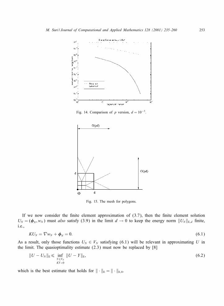
M. Suri / Journal of Computational and Applied Mathematics 128 (2001) 235–260 253
Fig. 14. Comparison of p version, d = 10−3.
Fig. 15. The mesh for polygons.
If we now consider the $nite element approximation of (3.7), then the $nite element solutionUN = (�N ; wN ) must also satisfy (3.9) in the limit d → 0 to keep the energy norm ‖UN‖E; d $nite,i.e.,
KUN =�wN + �N = 0: (6.1)
As a result, only those functions UN ∈ VN satisfying (6.1) will be relevant in approximating U inthe limit. The quasioptimality estimate (2.3) must now be replaced by [8]
‖U − UN‖E6 infY∈VN
KY=0
‖U − Y‖E; (6.2)
which is the best estimate that holds for ‖ · ‖E = ‖ · ‖E;0.
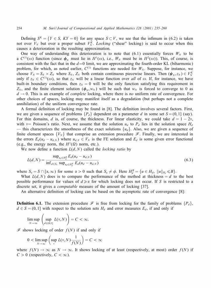
254 M. Suri / Journal of Computational and Applied Mathematics 128 (2001) 235–260
De$ning SK = {Y ∈ S; KY = 0} for any space S ⊂V , we see that the in$mum in (6.2) is takennot over VN but over a proper subset VK
N . Locking (“shear” locking) is said to occur when thiscauses a deterioration in the resulting approximation.
One way of understanding this deterioration is to note that (6.1) essentially forces WN to bea C(1)(!) function (since �N must lie in H 1(!), i.e., WN must be in H 2(!)). This, of course, isconsistent with the fact that in the d=0 limit, we are approximating the fourth-order KL (biharmonic)problem, for which, as noted earlier, C(1) functions are needed for WN . Suppose, for instance, wechoose VN = SN × ZN where SN , ZN both contain continuous piecewise linears. Then ( N ; zN ) ∈ VK
N
only if zN ∈ C(1)(!), so that zN will be a linear function over all of !. If, for instance, we havebuilt-in boundary conditions, then zN = 0 will be the only function satisfying this requirement inZN , and the $nite element solution (�N ; wN ) will be such that wN is forced to converge to 0 asd→ 0. This is an example of complete locking, where there is no uniform rate of convergence. Forother choices of spaces, locking may manifest itself as a degradation (but perhaps not a completeannihilation) of the uniform convergence rate.
A formal de$nition of locking may be found in [8]. The de$nition involves several factors. First,we are given a sequence of problems {Pd} dependent on a parameter d in some set S = (0; 1] (say).For thin domains, d is, of course, the thickness. For linear elasticity, we could take d = 1 − 2%,with %= Poisson’s ratio. Next, we assume that the solution ud to Pd lies in the solution space Hd
— this characterizes the smoothness of the exact solutions {ud}. Also, we are given a sequence of$nite element spaces {VN} that comprise an extension procedure F. Finally, we are interested inthe errors Ed(ud − ud;N ) where ud;N ∈ VN is the FE solution and Ed is some given error functional(e.g., the energy norm, the H 1(�) norm, etc.).
We now de$ne a function L(d; N ) called the locking ratio by
L(d; N ) =supud∈HB
dEd(ud − ud;N )
inf d∈S� supud∈HBdEd(ud − ud;N )
(6.3)
where S� = S ∩ [�;∞) for some �¿ 0 such that S� = *. Here HBd = {u ∈ Hd; ‖u‖Hd6B}.
What L(d; N ) does is to compare the performance of the method at thickness = d to the bestpossible performance for values of d¿� for which locking does not occur. If S is restricted to adiscrete set, it gives a computable measure of the amount of locking [37].
An alternative de$nition of locking can be based on the asymptotic rate of convergence [8]:
De�nition 6.1. The extension procedure F is free from locking for the family of problems {Pd},d ∈ S = (0; 1] with respect to the solution sets Hd and error measures Ed, if and only if
lim supN→∞
(sup
d∈(0;1]L(%; N )
)= C ¡∞:
F shows locking of order f(N ) if and only if
0¡ lim supN→∞
(sup%
L(%; N )1
f(N )
)= C ¡∞
where f(N ) → ∞ as N → ∞. It shows locking of at least (respectively, at most) order f(N ) ifC ¿ 0 (respectively, C ¡∞).
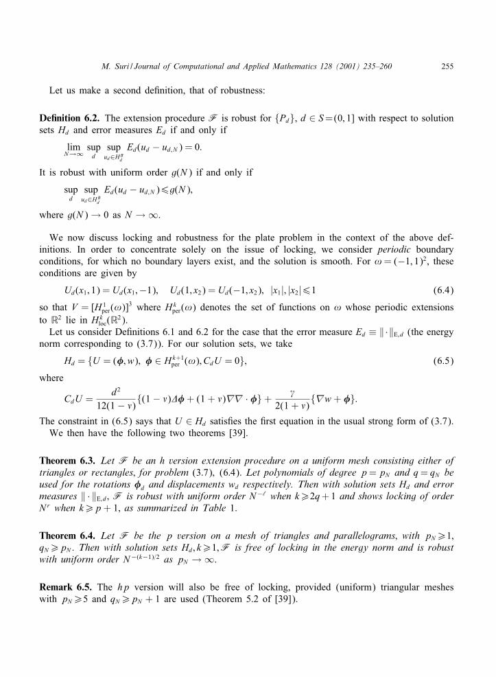
M. Suri / Journal of Computational and Applied Mathematics 128 (2001) 235–260 255
Let us make a second de$nition, that of robustness:
De�nition 6.2. The extension procedure F is robust for {Pd}, d ∈ S=(0; 1] with respect to solutionsets Hd and error measures Ed if and only if
limN→∞
supd
supud∈HB
d
Ed(ud − ud;N ) = 0:
It is robust with uniform order g(N ) if and only if
supd
supud∈HB
d
Ed(ud − ud;N )6g(N );
where g(N )→ 0 as N →∞.
We now discuss locking and robustness for the plate problem in the context of the above def-initions. In order to concentrate solely on the issue of locking, we consider periodic boundaryconditions, for which no boundary layers exist, and the solution is smooth. For ! = (−1; 1)2, theseconditions are given by
Ud(x1; 1) = Ud(x1;−1); Ud(1; x2) = Ud(−1; x2); |x1|; |x2|61 (6.4)
so that V = [H 1per(!)]3 where Hk
per(!) denotes the set of functions on ! whose periodic extensionsto R2 lie in Hk
loc(R2).Let us consider De$nitions 6.1 and 6.2 for the case that the error measure Ed ≡ ‖·‖E; d (the energy
norm corresponding to (3.7)). For our solution sets, we take
Hd = {U = (�; w); � ∈ Hk+1per (!); CdU = 0}; (6.5)
where
CdU =d2
12(1− %){(1− %)C� + (1 + %)�� · �}+
/2(1 + %)
{�w + �}:
The constraint in (6.5) says that U ∈ Hd satis$es the $rst equation in the usual strong form of (3.7).We then have the following two theorems [39].
Theorem 6.3. Let F be an h version extension procedure on a uniform mesh consisting either oftriangles or rectangles; for problem (3:7); (6:4). Let polynomials of degree p = pN and q = qN beused for the rotations �d and displacements wd respectively. Then with solution sets Hd and errormeasures ‖ · ‖E; d; F is robust with uniform order N−‘ when k¿2q+ 1 and shows locking of orderNr when k¿p + 1; as summarized in Table 1.
Theorem 6.4. Let F be the p version on a mesh of triangles and parallelograms; with pN¿1;qN¿pN . Then with solution sets Hd; k¿1;F is free of locking in the energy norm and is robustwith uniform order N−(k−1)=2 as pN →∞.
Remark 6.5. The hp version will also be free of locking, provided (uniform) triangular mesheswith pN¿5 and qN¿pN + 1 are used (Theorem 5.2 of [39]).
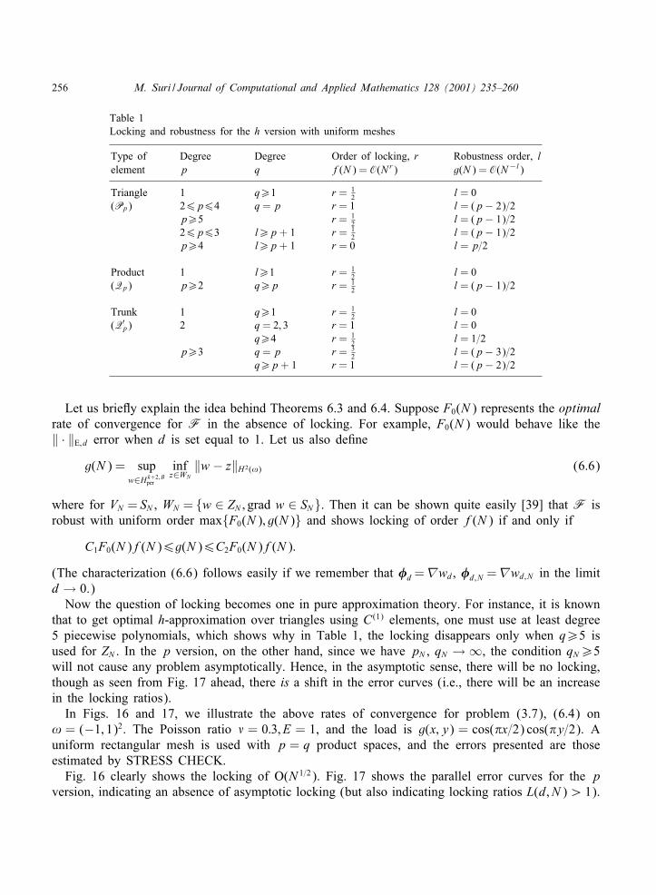
256 M. Suri / Journal of Computational and Applied Mathematics 128 (2001) 235–260
Table 1Locking and robustness for the h version with uniform meshes
Type of Degree Degree Order of locking, r Robustness order, lelement p q f(N ) = O(Nr) g(N ) = O(N−l)
Triangle 1 q¿1 r = 12 l = 0
(Pp) 26p64 q = p r = 1 l = (p− 2)=2p¿5 r = 1
2 l = (p− 1)=226p63 l¿p + 1 r = 1
2 l = (p− 1)=2p¿4 l¿p + 1 r = 0 l = p=2
Product 1 l¿1 r = 12 l = 0
(Qp) p¿2 q¿p r = 12 l = (p− 1)=2
Trunk 1 q¿1 r = 12 l = 0
(Q′p) 2 q = 2; 3 r = 1 l = 0
q¿4 r = 12 l = 1=2
p¿3 q = p r = 32 l = (p− 3)=2
q¿p + 1 r = 1 l = (p− 2)=2
Let us brie/y explain the idea behind Theorems 6.3 and 6.4. Suppose F0(N ) represents the optimalrate of convergence for F in the absence of locking. For example, F0(N ) would behave like the‖ · ‖E; d error when d is set equal to 1. Let us also de$ne
g(N ) = supw∈Hk+2; B
per
infz∈WN
‖w − z‖H 2(!) (6.6)
where for VN = SN , WN = {w ∈ ZN ; grad w ∈ SN}. Then it can be shown quite easily [39] that F isrobust with uniform order max{F0(N ); g(N )} and shows locking of order f(N ) if and only if
C1F0(N )f(N )6g(N )6C2F0(N )f(N ):
(The characterization (6.6) follows easily if we remember that �d =�wd, �d;N =�wd;N in the limitd→ 0.)
Now the question of locking becomes one in pure approximation theory. For instance, it is knownthat to get optimal h-approximation over triangles using C(1) elements, one must use at least degree5 piecewise polynomials, which shows why in Table 1, the locking disappears only when q¿5 isused for ZN . In the p version, on the other hand, since we have pN , qN →∞, the condition qN¿5will not cause any problem asymptotically. Hence, in the asymptotic sense, there will be no locking,though as seen from Fig. 17 ahead, there is a shift in the error curves (i.e., there will be an increasein the locking ratios).
In Figs. 16 and 17, we illustrate the above rates of convergence for problem (3.7), (6.4) on! = (−1; 1)2. The Poisson ratio % = 0:3; E = 1, and the load is g(x; y) = cos(Ex=2) cos(Ey=2). Auniform rectangular mesh is used with p = q product spaces, and the errors presented are thoseestimated by STRESS CHECK.
Fig. 16 clearly shows the locking of O(N 1=2). Fig. 17 shows the parallel error curves for the pversion, indicating an absence of asymptotic locking (but also indicating locking ratios L(d; N )¿ 1).
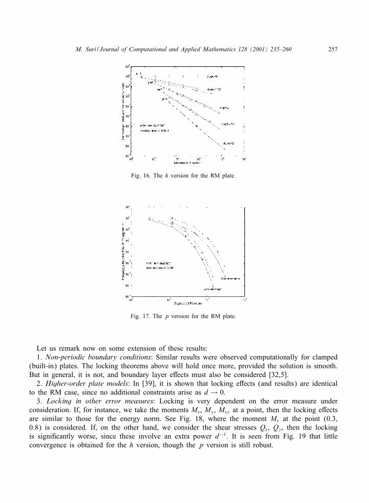
M. Suri / Journal of Computational and Applied Mathematics 128 (2001) 235–260 257
Fig. 16. The h version for the RM plate.
Fig. 17. The p version for the RM plate.
Let us remark now on some extension of these results:1. Non-periodic boundary conditions: Similar results were observed computationally for clamped
(built-in) plates. The locking theorems above will hold once more, provided the solution is smooth.But in general, it is not, and boundary layer eKects must also be considered [32,5].
2. Higher-order plate models: In [39], it is shown that locking eKects (and results) are identicalto the RM case, since no additional constraints arise as d→ 0.
3. Locking in other error measures: Locking is very dependent on the error measure underconsideration. If, for instance, we take the moments Mx, My, Mxy at a point, then the locking eKectsare similar to those for the energy norm. See Fig. 18, where the moment Mx at the point (0.3,0.8) is considered. If, on the other hand, we consider the shear stresses Qx, Qy, then the lockingis signi$cantly worse, since these involve an extra power d−1. It is seen from Fig. 19 that littleconvergence is obtained for the h version, though the p version is still robust.
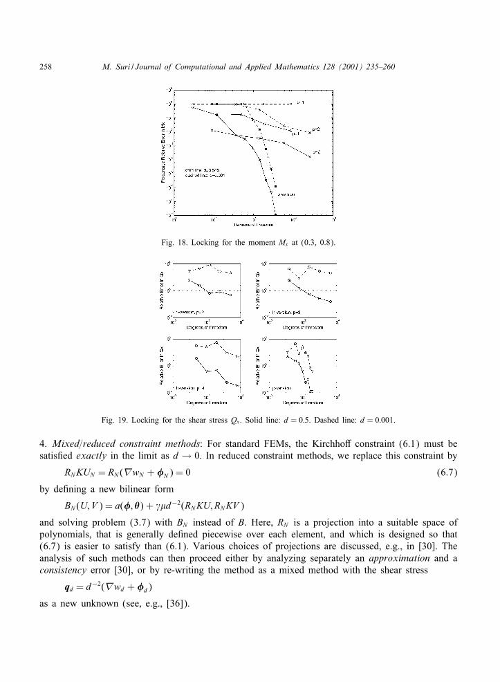
258 M. Suri / Journal of Computational and Applied Mathematics 128 (2001) 235–260
Fig. 18. Locking for the moment Mx at (0.3, 0.8).
Fig. 19. Locking for the shear stress Qx. Solid line: d = 0:5. Dashed line: d = 0:001.
4. Mixed=reduced constraint methods: For standard FEMs, the KirchhoK constraint (6.1) must besatis$ed exactly in the limit as d→ 0. In reduced constraint methods, we replace this constraint by
RNKUN = RN (�wN + �N ) = 0 (6.7)
by de$ning a new bilinear form
BN (U; V ) = a(�; �) + /�d−2(RNKU; RNKV )
and solving problem (3.7) with BN instead of B. Here, RN is a projection into a suitable space ofpolynomials, that is generally de$ned piecewise over each element, and which is designed so that(6.7) is easier to satisfy than (6.1). Various choices of projections are discussed, e.g., in [30]. Theanalysis of such methods can then proceed either by analyzing separately an approximation and aconsistency error [30], or by re-writing the method as a mixed method with the shear stress
qd = d−2(�wd + �d)
as a new unknown (see, e.g., [36]).
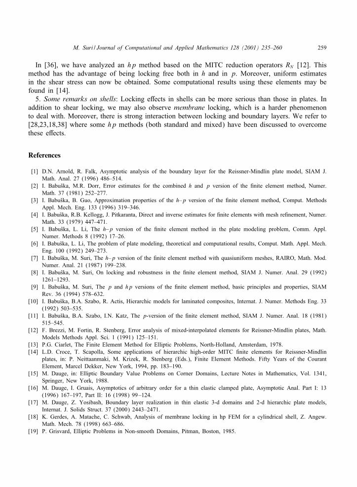
M. Suri / Journal of Computational and Applied Mathematics 128 (2001) 235–260 259
In [36], we have analyzed an hp method based on the MITC reduction operators RN [12]. Thismethod has the advantage of being locking free both in h and in p. Moreover, uniform estimatesin the shear stress can now be obtained. Some computational results using these elements may befound in [14].
5. Some remarks on shells: Locking eKects in shells can be more serious than those in plates. Inaddition to shear locking, we may also observe membrane locking, which is a harder phenomenonto deal with. Moreover, there is strong interaction between locking and boundary layers. We refer to[28,23,18,38] where some hp methods (both standard and mixed) have been discussed to overcomethese eKects.
References
[1] D.N. Arnold, R. Falk, Asymptotic analysis of the boundary layer for the Reissner-Mindlin plate model, SIAM J.Math. Anal. 27 (1996) 486–514.
[2] I. BabuGska, M.R. Dorr, Error estimates for the combined h and p version of the $nite element method, Numer.Math. 37 (1981) 252–277.
[3] I. BabuGska, B. Guo, Approximation properties of the h–p version of the $nite element method, Comput. MethodsAppl. Mech. Eng. 133 (1996) 319–346.
[4] I. BabuGska, R.B. Kellogg, J. Pitkaranta, Direct and inverse estimates for $nite elements with mesh re$nement, Numer.Math. 33 (1979) 447–471.
[5] I. BabuGska, L. Li, The h–p version of the $nite element method in the plate modeling problem, Comm. Appl.Numer. Methods 8 (1992) 17–26.
[6] I. BabuGska, L. Li, The problem of plate modeling, theoretical and computational results, Comput. Math. Appl. Mech.Eng. 100 (1992) 249–273.
[7] I. BabuGska, M. Suri, The h–p version of the $nite element method with quasiuniform meshes, RAIRO, Math. Mod.Numer. Anal. 21 (1987) 199–238.
[8] I. BabuGska, M. Suri, On locking and robustness in the $nite element method, SIAM J. Numer. Anal. 29 (1992)1261–1293.
[9] I. BabuGska, M. Suri, The p and hp versions of the $nite element method, basic principles and properties, SIAMRev. 36 (1994) 578–632.
[10] I. BabuGska, B.A. Szabo, R. Actis, Hierarchic models for laminated composites, Internat. J. Numer. Methods Eng. 33(1992) 503–535.
[11] I. BabuGska, B.A. Szabo, I.N. Katz, The p-version of the $nite element method, SIAM J. Numer. Anal. 18 (1981)515–545.
[12] F. Brezzi, M. Fortin, R. Stenberg, Error analysis of mixed-interpolated elements for Reissner-Mindlin plates, Math.Models Methods Appl. Sci. 1 (1991) 125–151.
[13] P.G. Ciarlet, The Finite Element Method for Elliptic Problems, North-Holland, Amsterdam, 1978.[14] L.D. Croce, T. Scapolla, Some applications of hierarchic high-order MITC $nite elements for Reissner-Mindlin
plates, in: P. Neittaanmaki, M. Krizek, R. Stenberg (Eds.), Finite Element Methods. Fifty Years of the CourantElement, Marcel Dekker, New York, 1994, pp. 183–190.
[15] M. Dauge, in: Elliptic Boundary Value Problems on Corner Domains, Lecture Notes in Mathematics, Vol. 1341,Springer, New York, 1988.
[16] M. Dauge, I. Gruais, Asymptotics of arbitrary order for a thin elastic clamped plate, Asymptotic Anal. Part I: 13(1996) 167–197, Part II: 16 (1998) 99–124.
[17] M. Dauge, Z. Yosibash, Boundary layer realization in thin elastic 3-d domains and 2-d hierarchic plate models,Internat. J. Solids Struct. 37 (2000) 2443–2471.
[18] K. Gerdes, A. Matache, C. Schwab, Analysis of membrane locking in hp FEM for a cylindrical shell, Z. Angew.Math. Mech. 78 (1998) 663–686.
[19] P. Grisvard, Elliptic Problems in Non-smooth Domains, Pitman, Boston, 1985.
260 M. Suri / Journal of Computational and Applied Mathematics 128 (2001) 235–260
[20] W. Gui, I. BabuGska, The h, p and h–p versions of the $nite element method in one dimension (Parts 1–3), Numer.Math. 40 (1986) 577–683.
[21] B. Guo, I. BabuGska, The h–p version of the $nite element method I and II, Comput. Mech. 1 (1986) 21–41 and203–226.
[22] H. Hakula, Licentiate Thesis, Helsinki University of Technology, 1997.[23] H. Hakula, Y. Leino, J. Pitkaranta, Scale resolution, locking, and high-order $nite element modeling of shells,
Comput. Methods Appl. Mech. Eng. 133 (1996) 157–182.[24] H. Han, R.B. Kellogg, DiKerentiability properties of solutions of the equation −&2Xu + ru = f(x; y) in a square,
SIAM J. Math. Anal. 21 (1990) 394–408.[25] R.B. Kellogg, Boundary layers and corner singularities for a self-adjoint problem, in: M. Costabel, M. Dauge,
S. Nicaise (Eds.), Lecture Notes in Pure and Applied Mathematics, Vol. 167, Marcel Dekker, New York, 1995, pp.121–149.
[26] V.A. Kondrat’ev, Boundary value problems for elliptic equations in domains with conic or corner points, Trans.Moscow Math. Soc. 16 (1967) 227–313.
[27] J.M. Melenk, C. Schwab, hp FEM for reaction-diKusion equations I: robust exponential convergence, SIAM J.Numer. Anal. 35 (1998) 1520–1557.
[28] J. Pitkaranta, The problem of membrane locking in $nite element analysis of cylindrical shells, Numer. Math. 61(1992) 523–542.
[29] J. Pitkaranta, Y. Leino, O. Ovaskainen, J. Piila, Shell deformation states and the $nite element method: A benchmarkstudy of cylindrical shells, Comput. Methods Appl. Mech. Eng. 128 (1995) 81–121.
[30] J. Pitkaranta, M. Suri, Design principles and error analysis for reduced-shear plate-bending $nite elements, Numer.Math. 75 (1996) 223–266.
[31] C. Schwab, p- and hp- Finite Element Methods, Oxford Science Publications, Oxford, 1998.[32] C. Schwab, M. Suri, Locking and boundary layer eKects in the $nite element approximation of the Reissner–Mindlin
plate model, Proc. Sympos. Appl. Math. 48 (1994) 367–371.[33] C. Schwab, M. Suri, The p and hp version of the $nite element method for problems with boundary layers, Math.
Comp. 65 (1996) 1403–1429.[34] C. Schwab, M. Suri, C. Xenophontos, The hp $nite element method for problems in mechanics with boundary
layers, Comput. Methods Appl. Mech. Eng. 157 (1998) 311–333.[35] G.I. Shishkin, Grid approximation of singularly perturbed parabolic equations with internal layers, Soviet J. Numer.
Anal. Math. Modelling 3 (1988) 393–407.[36] R. Stenberg, M. Suri, An hp error analysis of MITC plate elements, SIAM J. Numer. Anal. 34 (1997) 544–568.[37] M. Suri, Analytical and computational assessment of locking in the hp $nite element method, Comput. Methods
Appl. Mech. Eng. 133 (1996) 347–371.[38] M. Suri, A reduced constraint hp $nite element method for shell problems, Math. Comp. 66 (1997) 15–29.[39] M. Suri, I. BabuGska, C. Schwab, Locking eKects in the $nite element approximation of plate models, Math. Comp.
64 (1995) 461–482.[40] B.A. Szabo, I. BabuGska, Finite Element Analysis, Wiley, New York, 1991.[41] B.A. Szabo, A.K. Mehta, p-convergent $nite element approximations in fracture mechanics, Internat. J. Numer.
Methods Eng. 12 (1978) 551–560.[42] M.J. Turner, R.W. Clough, H.C. Martin, L.J. Topp, StiKness and de/ection analysis of complex structures, J.
Aeronaut. Sci. 23 (1956) 805–823.[43] R. Vulanovi[c, D. Herceg, N. Petrovi[c, On the extrapolation for a singularly perturbed boundary value problem,
Computing 36 (1986) 69–79.[44] C. Xenophontos, The hp version of the $nite element method for singularly perturbed boundary value problems,
Doctoral Dissertation, University of Maryland, Baltimore County, May 1996.[45] C. Xenophontos, The hp $nite element method for singularly perturbed problems in smooth domains, Math. Models
Methods Appl. Sci. 8 (1998) 299–326.[46] C. Xenophontos, Finite element computations for the Reissner–Mindlin plate model, Comm. Numer. Methods Eng.
14 (1998) 1119–1131.[47] C. Xenophontos, The hp $nite element method for singularly perturbed problems in nonsmooth domains, Numer.
Methods PDEs 27 (1999) 63–89.

Journal of Computational and Applied Mathematics 128 (2001) 261–279www.elsevier.nl/locate/cam
E$cient preconditioning of the linearized Navier–Stokesequations for incompressible ,ow
David Silvestera ;∗, Howard Elmanb, David Kayc, Andrew Wathend
aDepartment of Mathematics, UMIST, Manchester M60 1QD, UKbComputer Science Department and Institute of Advanced Computer Studies, University of Maryland, College Park,
MD 20742, USAcSchool of Mathematical Sciences, University of Sussex, Brighton BN1 9QH, UKdOxford University Computing Laboratory, Parks Road, Oxford OX1 3QD, UK
Received 14 October 1999; received in revised form 25 January 2000
Abstract
We outline a new class of robust and e$cient methods for solving subproblems that arise in the linearization andoperator splitting of Navier–Stokes equations. We describe a very general strategy for preconditioning that has two basicbuilding blocks; a multigrid V-cycle for the scalar convection–di:usion operator, and a multigrid V-cycle for a pressurePoisson operator. We present numerical experiments illustrating that a simple implementation of our approach leads toan e:ective and robust solver strategy in that the convergence rate is independent of the grid, robust with respect to thetime-step, and only deteriorates very slowly as the Reynolds number is increased. c© 2001 Elsevier Science B.V. Allrights reserved.
Keywords: Navier–Stokes equations; Incompressible ,ow; Preconditioning; Multigrid iteration
1. Introduction
The underlying goal here is to compute solutions of incompressible ,ow problems modelled bythe Navier–Stokes equations in a ,ow domain �⊂Rd (d = 2 or 3) with a piecewise smoothboundary @�:
@u@t
+ u ·�u − ��2u +�p = 0 in W ≡ � × (0; T ); (1.1)
� · u = 0 in W; (1.2)
∗ Corresponding author. Tel.: +44-161-200-3656; fax: +44-161-200-3669.E-mail address: [email protected] (D. Silvester).
0377-0427/01/$ - see front matter c© 2001 Elsevier Science B.V. All rights reserved.PII: S 0377-0427(00)00515-X

262 D. Silvester et al. / Journal of Computational and Applied Mathematics 128 (2001) 261–279
together with boundary and initial conditions of the form
u(x; t) = g(x; t) on GW ≡ @� × [0; T ]; (1.3)
u(x; 0) = u0(x) in �: (1.4)
We use standard notation: u is the ,uid velocity, p is the pressure, �¿ 0 is a speciJed viscosityparameter (in a nondimensional setting it is the inverse of the Reynolds number), and T ¿ 0 is someJnal time. The initial velocity Jeld u0 is typically assumed to satisfy the incompressibility constraint,that is, � · u0 = 0. The boundary velocity Jeld satisJes
∫@� g · n ds = 0 for all time t, where n is the
unit vector normal to @�.If the aim is to simply compute steady-state solutions of (1.1)–(1.2) then time accuracy is not
an issue. In other cases however, having an accurate solution at each time-step is important andthe requirements of the time discretisation will be more demanding; speciJcally, an accurate andunconditionally stable time-discretisation method is necessary to adaptively change the time-step tore,ect the dynamics of the underlying ,ow. We will not attempt to describe the many possibilities— the recent monographs of Gresho and Sani [14] and Turek [29] are worth consulting in thisrespect — but will restrict attention here to the simplest unconditionally stable approach using aone-stage Jnite di:erence discretisation, as given below.
Algorithm 1. Given u0; � ∈ [1=2; 1]; >nd u1; u2; : : : ; un via
(un+1 − un)Mt
+ u∗ ·� un+� − ��2un+� +�pn+� = 0;
� · un+� = 0 in �;
un+� = gn+� on @�:
(1.5)
Here un+� =�un+1 +(1−�)un and pn+� =�pn+1 +(1−�)pn. Note that p0 is required if � �= 1 so theAlgorithm 1 is not self-starting in general. In this case an approximation to p0 must be computedexplicitly by manipulation of the continuum problem, or alternatively it must be approximated bytaking one (very small) step of a self-starting algorithm (e.g., with � = 1 above).
Algorithm 1 contains the well-known nonlinear schemes of backward Euler and Crank–Nicolson.These methods are given by (un+� = un+1; u∗ = un+1); (un+� = un+1=2; u∗ = un+1=2), and are Jrst andsecond-order accurate, respectively. In either case, a nonlinear problem must be solved at everytime-level. A well-known linearization strategy is to set u∗ = un above. This does not a:ect thestability properties of the time discretisation, but it does reduce the Crank–Nicolson accuracy to Jrstorder as Mt → 0 (the Jrst order accuracy of backward Euler is unchanged). To retain second-orderaccuracy in a linear scheme the Simo–Armero scheme [24] given by setting un+� = un+1=2 withu∗ = (3un − un−1)=2 in Algorithm 1 is recommended, see [26] for further details.
Using linearized backward Euler or the Simo-Armero scheme, a frozen-coe$cient Navier–Stokesproblem (or generalised Oseen problem) arises at each discrete time step: given a divergence-freevector Jeld w(x) (which we will refer to as the “wind”), the aim is to compute u(x) and p(x) suchthat
1Mt
u + w ·�u − ��2u +�p = f in � (1.6)
D. Silvester et al. / Journal of Computational and Applied Mathematics 128 (2001) 261–279 263
� · u = 0 in �; (1.7)
u = g on @�: (1.8)
Notice that since (1.6)–(1.8) represents a linear elliptic PDE problem, the existence and uniquenessof a solution (u; p) can be established under very general assumptions. The development of e$cientmethods for solving discrete analogues of (1.6)–(1.8) is the focal point of this work.
An outline is as follows. The spatial discretisation of the generalised Oseen problem is discussed inSection 2. Some standard Krylov iteration methods that are applicable to the (nonsymmetric-) systemsthat arise after discretisation are brie,y reviewed in Section 3. Our general preconditioning approachis then developed in Section 4. This approach builds on our research e:ort over the last decade ondeveloping e:ective preconditioners for limiting cases of the Oseen problem (1.6)–(1.8): speciJcallysteady-state Stokes problems (Mt → ∞; w → 0) [22]; generalised Stokes problems (w → 0), seeSilvester and Wathen [23]; and steady Oseen problems (Mt → ∞) [5,6,16]. Some computationalexperiments that demonstrate the power of our solution methodology are presented in Section 5.Implementation of “pure” multigrid methods seems to be relatively complicated, and performanceseems to be (discretisation-) method dependent by comparison. The derivation of analytic boundson convergence rates for the general preconditioner is an ongoing project which will be treated ina forthcoming paper [7]; in the Jnal section we give a ,avour of the analysis by quoting resultsthat we have established in two special cases; potential ,ow (w = 0 and � = 0) and generalisedStokes ,ow (w = 0). These cases typically arise using time-stepping methods for (1.1)–(1.2) basedon operator splitting — showing the inherent generality of the preconditioning approach.
2. Spatial discretisation
Given that we would like to solve our model problem (1.6)–(1.8) over irregular geometries,the spatial discretisation will be done using Jnite element approximation (this also gives us more,exibility in terms of adaptive reJnement via a posteriori error control, see, e.g., [17]). We note thatthe algorithm methodology discussed in the paper applies essentially verbatim to Jnite di:erence andJnite volume discretisations. In the remainder of this section we brie,y review the error analysisassociated with mixed Jnite element approximation of (1.6)–(1.8). For full details see [13].
The weak formulation of (1.6)–(1.8) is deJned in terms of the Sobolev spaces H 10 (�) (the
completion of C∞0 (�) in the norm || · ||1) and L2
0(�) (the set of functions in L2(�) with zero meanvalue on �). DeJning a velocity space X ≡ (H 1
0 (�))d and a pressure space M ≡ L20(�), it is easy
to see that the solution (u; p) of (1.6)–(1.8) satisJes
1Mt
(u; C) + (w ·�u; C) + �(�u;�C)− (p;� · C) = ( f ; C) ∀C ∈ X ; (2.1)
(� · u; q) = 0 ∀q ∈ M; (2.2)
where (·; ·) denotes the usual vector or scalar L2(�) inner product. Since � is bounded and connectedthere exists a constant � satisfying the continuous inf–sup condition:
supw∈X
(p;� · w)||w||1 ¿�||p|| ∀p ∈ M: (2.3)
264 D. Silvester et al. / Journal of Computational and Applied Mathematics 128 (2001) 261–279
Furthermore, since w is divergence-free, the bilinear form c(·; ·) given by
c(u; C) =1
Mt(u; C) + (w ·�u; C) + �(�u;�C) (2.4)
is coercive and bounded over X ;
c(C; C)¿�||�C||2 ∀C ∈ X ; (2.5)
|c(u; C)|6Cw||�u||||�C|| ∀u ∈ X ;∀ C ∈ X : (2.6)
Existence and uniqueness of a solution to (2.1)–(2.2) then follows from a generalisation of theusual Lax–Milgram lemma [13].
To generate a discrete system we take Jnite dimensional subspaces Xh⊂X and Mh⊂L2(�), whereh is a representative mesh parameter, and enforce (2.1)–(2.2) over the discrete subspaces (againspecifying that functions in Mh have zero mean to ensure uniqueness). SpeciJcally, we look for afunction uh satisfying the boundary condition (1.8), and a function ph ∈ Mh such that
1Mt
(uh; C) + (wh ·�uh; C) + �(�uh;�C)− (ph;� · C) = ( f ; C) ∀C ∈ Xh; (2.7)
(� · uh; q) = 0 ∀q ∈ Mh; (2.8)
where wh represents the interpolant of w in Xh. Notice that this approximation means that the discretewind is not actually pointwise divergence-free. From the linear algebra perspective the point is that inthe case of the enclosed ,ow boundary condition (1.3), the discrete convection matrix correspondingto the term (wh ·�uh; C) is skew symmetric.
The well-posedness of (2.7)–(2.8) is not automatic since we do not have an internal approxima-tion. A su$cient condition for the existence and uniqueness of a solution to (2.7)–(2.8) is that thefollowing discrete inf–sup condition is satisJed: there exists a constant � independent of h such that
supC∈Xh
(q;� · C)||�C|| ¿�||q|| ∀q ∈ Mh: (2.9)
Note that the semi-norm ||�C|| in (2.9) is equivalent to the norm ||C||1 for functions C ∈ X . Theinf–sup condition also guarantees optimal approximation in the sense of the error estimate [13]
||�(u − uh)||+ ||p− ph||6C(
infC∈Xh
||�(u − C)||+ infq∈Mh
||p− q||): (2.10)
Note that the constant C is inversely proportional to the inf–sup constant � in (2.9).Since we want to use linear algebra tools it is convenient to express the discrete problem (2.7)–
(2.8) as a matrix problem. To do this we introduce discrete operators F :Xh �→ Xh and B :Xh �→ Mh
deJned via
(FCh; zh) =1
Mt(Ch; zh) + (wh ·�Ch; zh) + �(�Ch;�zh) ∀Ch; zh ∈ Xh; (2.11)
(BCh; qh) = (Ch;B∗qh) =−(� · Ch; qh) ∀Ch ∈ Xh;∀qh ∈ Mh; (2.12)
so that B∗ is the adjoint of B. With these deJnitions the discrete problem (2.7)–(2.8) can berewritten as a matrix system: Jnd uh satisfying the boundary condition (1.8) such that(
F B∗
B 0
)(uh
ph
)=(f0
): (2.13)
D. Silvester et al. / Journal of Computational and Applied Mathematics 128 (2001) 261–279 265
Furthermore, introducing A :Xh �→ Xh, satisfying
(ACh; zh) = (�Ch;�zh) ∀Ch; zh ∈ Xh; (2.14)
the inf–sup inequality (2.9) simpliJes to
�||qh||6 supCh∈Xh
(BCh; qh)(ACh; Ch)1=2
∀qh ∈ Mh: (2.15)
It is instructive to express (2.13) and (2.15) in terms of the actual Jnite element matrices thatarise in practice. To this end, let us explicitly introduce the Jnite element basis sets, say,
Xh = span{�i}ni=1; Mh = span{ j}mj=1; (2.16)
and associate the functions uh, ph, with the vectors u ∈ Rn; p ∈ Rm of generalised coe$-cients, ph =
∑mj=1 pj j, etc. DeJning the n × n “convection”, “di:usion” and “mass” matrices
Nij = (wh · ��i; �j); Aij = (��i;��j) and Gij = (�i; �j), and also the m × n “divergence matrix”Bij =−(� :�j; i), gives the Jnite element version of (2.13):( 1
Mt G + N + �A Bt
B 0
)(up
)=(fg
); (2.17)
where the RHS term g arises from enforcement of the (non-homogeneous) boundary condition onthe function uh; see [14, pp. 440–448] for details.
Moreover, introducing the m×m pressure “mass” matrix Qij = ( i; j); leads to the Jnite elementversion of (2.9): for all p ∈ Rm,
�(ptQp)1=26maxu
ptBu(utAu)1=2
(2.18)
= maxw=A1=2u
ptBA−1=2w(wtw)1=2
(2.19)
= (ptBA−1Btp)1=2; (2.20)
since the maximum is attained when w = A−1=2Btp. Thus, we have a characterization of the inf–supconstant:
�2 = minp �=0
ptBA−1BtpptQp
: (2.21)
In simple terms it is precisely the square root of the smallest eigenvalue of the preconditioned Schurcomplement Q−1BA−1Bt . We also have that
(q;� · C)6||q|| ||� · C||6√d||q|| ||�C|| (2.22)
where �⊂Rd, and so there also exists a constant '6√d satisfying
'2 = maxp �=0
ptBA−1BtpptQp
: (2.23)
Note that the tight bound '61 was recently established (valid in the case of a conforming approx-imation space, Xh⊂X) by Stoyan [28].

266 D. Silvester et al. / Journal of Computational and Applied Mathematics 128 (2001) 261–279
In practice, the inf–sup condition (2.9) is extremely restrictive. Problems arise if the pressurespace Mh is too rich compared to the velocity space Xh. Although many stable methods have beendeveloped (see [14] for a complete list of possibilities), many natural low order conforming Jniteelement methods like Q1–P0 (trilinear/bilinear velocity with constant pressure) are unstable in thesense that pressure vectors p ∈ Mh can be constructed for which the inf–sup constant tends to zerounder uniform grid reJnement. This type of instability can be di$cult to detect in practice since theassociated discrete systems (2.17) are all nonsingular — so that every discrete problem is uniquelysolvable — however they become ill-conditioned as h→ 0.
Another issue, which needs to be addressed when applying multigrid solution techniques toconvection–di:usion problems of the form
c(uh; C) = ( fh; C) ∀C ∈ Xh; (2.24)
(with c(·; ·) given by (2.4)), is that standard approximation methods may produce an unstable,possibly oscillating, solution if the mesh is too coarse in critical regions. In such cases, to giveadditional stability on coarse meshes used in the multigrid process, the discrete problem (2.24)needs to be stabilised. For example, using a streamline-di?usion method, we replace (2.24) by theregularised problem
c(uh; C) + )(wh ·�uh;wh ·�C) = ( fh; C) ∀C ∈ Xh; (2.25)
where ) is a locally deJned stabilisation parameter, see [15] for further details.The formulation (2.25) clearly has better stability properties than (2.24) since there is additional
coercivity in the local ,ow direction. The local mesh PTeclet number PeT = ||wh||∞; T hT =� determines
the streamline-di:usion coe$cient )T in a given element T via the “optimal” formula [10];
)T =
12hT (1− 1
PeT) if Pe
T ¿ 1;
0 if PeT61;
(2.26)
where hT is a measure of the element length in the direction of the wind.
3. Krylov subspace solvers
Let Lx = f denote a generic linear system of equations. Krylov subspace solution methods startwith a guess x(0) for the solution, with residual r(0) = f − Lx(0), and construct a sequence ofapproximate solutions of the form
x(k) = x(0) + p(k) (3.1)
where p(k) is in the k-dimensional Krylov space
Kk(r(0);L) = span{r(0);Lr(0); : : : ;Lk−1r(0)}:In this section, we give a brief overview of properties of Krylov subspace methods for solving thesystems arising from the discretizations discussed in the previous section.
Problem (2.17) is nonsymmetric so that algorithms applicable to such problems are of primaryconcern, but the small Reynolds number limit leads to a symmetric indeJnite Stokes problem, and weJrst brie,y discuss this case. It is well-known that for symmetric indeJnite problems, the MINRES
D. Silvester et al. / Journal of Computational and Applied Mathematics 128 (2001) 261–279 267
algorithm [20] generates iterates of the form (3.1) for which the residual r(k) has minimal Euclideannorm. It follows that the residuals satisfy
||r(k)||2||r(0)||26 min
�k (0)=1max
.∈/(L)|�k(.)|;
where the minimum is taken over polynomials �k of degree k satisfying �k(0) = 1. This result leadsto the following bound on the relative residual norm [18].
Theorem 3.1. If the eigenvalues of L are contained in two intervals [ − a;−b] ∪ [c; d] witha− b = d− c¿ 0; then the residuals generated by MINRES satisfy
||r(k)||2||r(0)||262
(1−√21 +
√2
)k=2
;
where 2 = (bc)=(ad).
We apply this result to the Stokes equations in the Jnal section. We also point out that tighterbounds can be established when a − b �= d − c and b; d have some asymptotic behaviour, [32,33].Each step of the computation entails only a matrix–vector product together with a small number,independent of the iteration count, of vector operations (scalar-vector products and inner products),so that the cost per step of the MINRES iteration is low.
For nonsymmetric problems, there is no Krylov subspace solver that is optimal with respect tosome error norm for which the cost per step is independent of the iteration count [8,9]. The gener-alized minimal residual algorithm (GMRES) [21] is the most e$cient “optimal” solver, producingthe unique iterate of the form (3.1) for which the Euclidean norm of the residual is smallest. Stepk requires one matrix–vector product together with a set of k vector operations, making its cost, interms of both operation counts and storage, proportional to kN where N is the problem dimension.We summarize the main convergence properties of GMRES below. See [4,21] for proofs.
Theorem 3.2. Let x(k) denote the iterate generated after k steps of GMRES; with residual r(k) =f −Lx(k).
(i) The residual norms satisfy ||r(k)||2 = min�k (0)=1||�k(L)r(0)||2.(ii) If L = X3X−1 is diagonalizable; where 3 is the diagonal matrix of eigenvalues of L; then
||r(k)||26||X ||2 ||X−1||2 min�k (0)=1
max.j|�k(.j)| ||r(0)||2:
Assertions (i) and (ii) follow from the optimality of GMRES with respect to the residual norm.Assertion (i) guarantees that GMRES will solve any nonsingular problem provided that the dimen-sions of the Krylov space is large enough. This di:erentiates GMRES from most other nonsymmetricKrylov subspace methods.
The GMRES iterate is computed as in (3.1) with p(k) of the form p(k) = Vky(k), where Vk isa matrix whose columns form an orthogonal basis for Kk . The construction of the orthogonalbasis is what makes the cost per step high, but once such a basis is available, the iterate withsmallest residual norm can be computed cheaply. See [21] for details. Nonoptimal methods com-promise on these points, reducing the cost per step by avoiding the construction of an orthogonal

268 D. Silvester et al. / Journal of Computational and Applied Mathematics 128 (2001) 261–279
basis, but thereby making the construction of an optimal iterate too expensive. Numerous methodsof this type have been proposed, for example, BiCGSTAB [30], BiCGSTAB (‘) [25], CGS [27],QMR [11].
The results of Theorems 3.1–3.2 indicate that if the eigenvalues of L are tightly clustered, thenconvergence will be rapid. In particular, for MINRES, it is desirable for the sizes of the twointervals (one on each side of the origin) to be as small as possible, and well separated fromthe origin. For GMRES, Theorem 3.2(ii) suggests that convergence will be fast if the eigenval-ues can be enclosed in a region in the complex plane that is small. The spectra of the dis-crete problems of Section 2 are not well-behaved in this sense, and convergence must be en-hanced by preconditioning. That is, we use an operator P ≈ L and solve an equivalent systemsuch as P−1Lx = P−1b, with a more favorable distribution of eigenvalues, by Krylov subspaceiteration.
We conclude this section with a few general observations concerning preconditioning for bothsymmetric indeJnite and nonsymmetric problems. Sections 4 and 6 discuss and analyze some speciJcstrategies suitable for (2.17). First, we note that preconditioning increases the cost per step, sincethe matrix–vector product now requires a preconditioning operation, i.e., application of the action ofP−1 to a vector. Thus, for the preconditioner to be e:ective, the improved convergence speed mustbe enough to compensate for the extra cost.
The MINRES algorithm can be combined with preconditioning by a symmetric positive-deJniteoperator P. Formally, MINRES is then applied to the symmetric matrix L = S−1LS−T , whereP = SSt . The error bound analogous to that of Theorem 3.1 is
||r(k)||P−1
||r(0)||P−162
(1−√21 +
√2
)k=2
; (3.2)
where the intervals deJning 2 now come from the eigenvalues of the preconditioned operator L.Thus, we seek a preconditioner for which the computation of the action of P−1 is inexpensive, andfor which the eigenvalues of L are tightly clustered, leading to smaller 2. Note also that the normin (3.2) is now di:erent; for further details see [23]. It is also possible to apply the QMR algorithmto symmetric indeJnite problems (with comparable complexity to that of MINRES). In this case asymmetric indeJnite preconditioner can be used [12].
For nonsymmetric problems, there is some ,exibility in how the preconditioned problem may beformulated, with three possible di:erent “orientations”:
Left orientation [P−1L] [x] = [P−1f];
Two-sided orientation [P−11 LP−1
2 ] [P2x] = [P−12 f];
Right orientation [LP−1] [Px] = [f]:
The two-sided orientation depends on having an explicit representation of the preconditioner infactored form P = P1P2. In our experience, there is little di:erence in the e:ectiveness of thesechoices. We tend to prefer the “right” variant, especially for use with GMRES, since the normbeing minimized (the Euclidian norm of the residual) is then independent of the choice of thepreconditioner.
D. Silvester et al. / Journal of Computational and Applied Mathematics 128 (2001) 261–279 269
4. Preconditioning strategy
Our starting point is the discrete system Lx = f associated with (2.17), which we write in theform (
F Bt
B 0
)(up
)=(fg
)(4.1)
so that F = (1=Mt)G + N + �A ∈ Rn×n, with B ∈ Rm×n. Our preconditioning strategy is based on theassumption that a fast solver (typically based on multigrid) is available for the convection–di:usionsystem Fu = f. This leads us to consider a block triangular preconditioning
P−1 =(F−1 R
0 −S−1
); (4.2)
with matrix operators R∈Rn×m and S ∈Rm×m chosen to provide clustering of the eigenvalues/(LP−1) of the right preconditioned system
LP−1 =(
In FR− BtS−1
BF−1 BR
): (4.3)
The speciJc choice of R and S in (4.2) satisfying
FR− BtS−1 = O; BR = Im;
that is, R = F−1BtS−1 with S = BF−1Bt , is the optimal choice, see [19]. For this choice, it followsfrom (4.3) that /(LP−1) = {1}, and preconditioned GMRES converges to the solution of (4.1) inat most two iterations.
Implementation of a right preconditioner for GMRES requires the solution of a system of theform Py = r at every step. (QMR also requires the solution of a system with Pt .) With the optimalchoice of R and S we need to compute the vector ( v
q ) satisfying(
vq
)=(F−1 F−1BtS−1
0 −S−1
)(rs
); (4.4)
for given vectors r ∈Rn, and s∈Rm. Rewriting (4.4) shows that the optimal preconditioner is deJnedby a two-stage process:
Solve for q : Sq =−s;Solve for v : Fv = r − Btq:
(4.5)
To get a practical method, we modify the preconditioning process (4.5) by replacing the matrixoperators S =BF−1Bt and F , by approximations S∗ and F∗ respectively, designed so that the precon-ditioned Oseen operator has a tightly clustered spectrum. We are particularly interested in operatorsS∗ and F∗ derived from multigrid computations such that /(SS−1
∗ ) ∈ !S and /(FF−1∗ ) ∈ !F where
!S and !F represent small convex sets in the right half of the complex plane; ideally, these setswould be independent of the problem parameters �, h, and Mt.
The construction of the operator F∗ ≈ F is relatively straightforward, see Section 5. The moredi$cult issue is the construction of a simple multigrid approximation to the Schur complement
270 D. Silvester et al. / Journal of Computational and Applied Mathematics 128 (2001) 261–279
BF−1Bt , see, e.g., [29, p. 56]. The approach presented here was developed by Kay and Loghin [16]and represents an improved version of ideas in [6,5].
To motivate the derivation, suppose for the moment that we have an unbounded domain, and thatdi:erential operators arising in (1.6)–(1.8) commute:
�(1=Mt + w ·� − ��2)p ≡ (1=Mt + w ·� − ��2)u� (4.6)
where for any operator >; >u represents the vector analogue of the scalar operator >p. If we furtherassume that a C0 pressure approximation is used (so that Mh⊂H 1(�)) then we can construct adiscrete pressure convection–di:usion operator Fp :Mh �→ Mh such that
(Fpqh; rh) =1
Mt(qh; rh) + (wh ·�qh; rh) + �(�qh;�rh) ∀qh; rh ∈ Mh: (4.7)
Introducing the L2-projection operators G :Xh �→ Xh and Q :Mh �→ Mh
(GCh; zh) = (Ch; zh) ∀Ch; zh ∈ Xh;
(Qqh; rh) = (qh; rh) ∀qh; rh ∈ Mh;
then gives the discrete analogue of (4.6)
(G−1B∗)(Q−1Fp) ≡ (G−1F)(G−1B∗): (4.8)
A simple rearrangement of (4.8) gives
(G−1F)−1(G−1B∗) ≡ (G−1B∗)(Q−1Fp)−1;
F−1B∗ ≡ G−1B∗F−1p Q:
Hence, assuming that (4.8) is valid, we have an alternative expression for the Schur complementoperator BF−1B∗ :Mh �→ Mh, namely
BF−1B∗ ≡ BG−1B∗F−1p Q: (4.9)
For equivalence (4.9) to hold, it is necessary for the spaces Xh and Mh to be deJned withperiodic boundary conditions. In the case of an enclosed ,ow boundary condition like (1.8), thediscrete operator Fp inherits natural boundary conditions (associated with the space M), and in thiscase (4.9) gives us a starting point for approximating the Schur complement matrix S = BF−1Bt .Using basis (2.16), we have the approximation
BG−1BtF−1p Q = PS ≈ S: (4.10)
The goal now is to design an e$cient implementation of a preconditioner based on (4.10). Thisrequires that fast solvers for the underlying operators Q and BG−1B∗ are available: we seek operatorsQ∗ and H∗ such that there exist constants �, >; .; 3 independent of h, satisfying
� 26ptQpptQ∗p
6>2 ∀p ∈ Rm; (4.11)
and
.26ptBG−1Btp
ptH∗p632 ∀p ∈ Rm; (4.12)
D. Silvester et al. / Journal of Computational and Applied Mathematics 128 (2001) 261–279 271
respectively. The practical version of the preconditioner is then deJned by replacing the action ofS−1 in the Jrst step of (4.5) by the so called Fp approximation:
S−1∗ = Q−1
∗ FpH−1∗ : (4.13)
Satisfying (4.11) is straightforward; the simple pressure scaling Q∗ = diag (Q) does the trick [31].The upshot is that the action of Q−1 in (4.10) can be approximated very accurately using a Jxed(small) number of steps of diagonally scaled conjugate gradient iteration applied to the operator Q.
Relation (4.12) can also be satisJed using a multigrid approach. The crucial point is that the useof a C0 pressure approximation space is associated with an alternative inf–sup condition, see, e.g.,[1]: for a stable mixed approximation there exists a constant 2 independent of h, such that
supC∈Xh
(C;�q)||C|| ¿2||�q|| ∀q ∈ Mh: (4.14)
Thus, introducing the pressure Laplacian operator Ap :Mh �→ Mh such that
(Apqh; rh) = (�qh;�rh) ∀qh; rh ∈ Mh;
we have that (4.14) is equivalent to
2(Apqh; qh)1=26 supCh∈Xh
(Ch;B∗qh)||Ch|| ∀qh ∈ Mh:
Applying the same arguments used to get (2.21) and (2.23), we have a natural characterization interms of the matrices associated with the Jnite element basis (2.16):
226ptBG−1Btp
ptApp61 ∀p ∈ Rm: (4.15)
In simple terms, for a stable mixed discretisation, the operator BG−1B∗ is spectrally equivalentto the Poisson operator Ap deJned on the pressure space Mh (with inherited Neumann boundaryconditions) [14, p. 563]. We note in passing that an equivalence of the form (4.15) can also holdin cases when a discontinuous pressure approximation is used (with an appropriately deJned matrixoperator Ap). For example, in the case of well known MAC discretization on a square grid, we haveAp = h−2BBt where Ap is the standard Jve-point Laplacian deJned at cell centres.
The result (4.15) opens up the possibility of using a multigrid preconditioner. In particular, a singlemultigrid V-cycle with point Jacobi or (symmetric) Gauss–Seidel smoothing deJnes an approximationH∗, with spectral bounds
�26ptAppptH∗p
61 ∀p ∈ Rm: (4.16)
The combination of (4.15) and (4.16) shows that a simple multigrid cycle can be used as anapproximation to BG−1B∗ in the sense that (4.12) holds with constants . = 2� and 3 = 1.
To end this section we would like to emphasize the simplicity of the practical implementation ofthe preconditioner associated with (4.5). The computation of q in the Jrst stage entails an approxima-tion of the action of P−1
S deJned by (4.10). This is done in three steps; the Jrst is the approximationto the action of the inverse of BG−1Bt using a multigrid iteration applied to a system with coe$-cient matrix Ap (typically representing a Poisson operator with Neumann boundary conditions), thesecond step is a matrix–vector product involving the discrete convection–di:usion operator Fp, and
272 D. Silvester et al. / Journal of Computational and Applied Mathematics 128 (2001) 261–279
the third step is essentially a scaling step corresponding to the solution of a system with coe$cientmatrix given by the pressure mass matrix Q. For the second stage of (4.5), the computation of v isapproximated by a multigrid iteration for the convection–di:usion equation. Clearly, the overall costof the preconditioner is determined by the cost of a convection–di:usion solve on the velocity spaceand of a Poisson solve on the pressure space; with multigrid used for each of these, the complexityis proportional to the problem size.
5. Computational results
We use P2–P1 mixed Jnite element approximation (see, e.g., [14, p. 462]), that is, we choosespaces
Xh = {v ∈ H 10 (�) : v|T ∈ P2(T ) ∀T ∈Th};
Mh = {q ∈ H 1(�) : q|T ∈ P1(T ) ∀T ∈Th};where T is a triangle in the mesh Th. (This mixed method is shown to be inf–sup stable in [1].) Werestrict attention to uniformly reJned meshes in this work, analogous results for adaptively reJnedmeshes are given in [16].
We present results for three standard test ,ow problems below. The time discretization is backwardEuler, and the linearization strategy is given by the choice u∗ = un in Algorithm 1. In all caseswe run the time integrator for 15 time-steps, unless the stopping criterion ||un+1 − un||2 ¡ 10−6 issatisJed. We solve the linear system that arises at each discrete time interval using GMRES with thepreconditioner P that is deJned below. The GMRES starting vector for the nth time-step is alwaystaken to be the previous time-step solution (un−1, pn−1). GMRES iterations are performed until therelative residual is reduced by 10−6.
We will denote the action of a single multigrid V-cycle using a point Gauss–Seidel smoother forthe discrete velocity operator F in (2.11), by F−1
∗ ; where we perform one smoothing sweep beforea Jne to coarse grid transfer of the residual, and one smoothing sweep after a coarse to Jne gridtransfer of the correction. For details see e.g., [34]. Similarly we let H−1
∗ denote the action of asingle multigrid V-cycle using damped Jacobi as a smoother (with damping parameter 0.8) for thepressure Laplacian operator Ap in (4.7) (again with a single sweep of pre- and post-smoothing).We comment that although the use of multigrid as a solver for a Laplacian operator is very robust,using a simple multigrid cycle with point smoothing does not generally lead to an e$cient solverfor the convection–di:usion operator F when convection dominates (although the same strategycan still be an e:ective preconditioner [34]). If we let Q−1
∗ denote two diagonally scaled conjugategradient iterations applied to the discrete pressure identity, then our inverse preconditioner is of theform:
P−1∗ =
(F−1∗ 00 I
)(I BT
0 −I)(
I 00 Q−1
∗ FpH−1∗
):
Within the multigrid process we construct prolongation operators using interpolation that is con-sistent with the order of the velocity=pressure approximation spaces. Furthermore, the restrictionoperator is the usual transpose of the prolongation, and on the coarsest level (h = 1=2 below) weperform an exact solve. Finally, we emphasize that if the local mesh PTeclet number is greater than

D. Silvester et al. / Journal of Computational and Applied Mathematics 128 (2001) 261–279 273
Table 1Nh
Mt for Stokes driven cavity ,ow
Mt h = 1=4 h = 1=8 h = 1=16
0.001 9 10 120.1 13 14 141 14 15 1510 14 15 151000 14 15 15
unity on any grid, then streamline di:usion is included in the discrete system that is solved (as wellas the discrete convection–di:usion problems deJning the operator F−1
∗ , see (2.26)).To show the robustness of our solver we report below the maximum number of GMRES iterations
required for the tolerance to be satisJed on a given mesh (with a given Mt) over all time iterations;this maximum iteration count is denoted by Nh
Mt .
5.1. Stokes: driven cavity Bow
We Jrstly consider the (symmetric-) generalized Stokes problem, associated with a standard drivencavity ,ow problem deJned on a unit domain �= (0; 1)× (0; 1). The associated boundary conditionis given by
u(@�; t) ={
(1; 0) y = 1;0 otherwise;
and we “spin-up” to the steady state from the initial condition u(x; 0) = 0.The performance of our preconditioned method is summarized in Table 1. These iteration counts
are consistent with our expectation that the rate of convergence is independent of the degree of meshreJnement, and the size of the time-step. We note that in the limit Mt →∞, the system reduces toa stationary Stokes system in which case we have tight analytic bounds showing the e:ectivenessof the same preconditioning strategy in a MINRES context, see Section 6.
5.2. Navier–Stokes: driven cavity Bow
We also consider the Navier–Stokes problem associated with the domain, boundary and initialconditions given above. These results are given in Table 2.
The obvious point to note here is that, as in the Stokes case, the performance is not a:ectedby mesh reJnement. (The trend is clearly evident even though the meshes are relatively coarse.) Incontrast to the results in the Stokes case it can be seen that as Mt gets larger in Table 2, the iterationcounts tend to an asymptotic maximum value. Moreover this maximum value becomes somewhatlarger as � is decreased. This behaviour is consistent with our expectations — steady-state iterationcounts that are presented in [16] can be seen to slowly increase as the Reynolds number is increased.A complete theoretical explanation is not yet available, but see [7].

274 D. Silvester et al. / Journal of Computational and Applied Mathematics 128 (2001) 261–279
Table 2Nh
Mt for Navier–Stokes driven cavity ,ow
h = 1=4 h = 1=8 h = 1=16
� = 1=50Mt = 0:1 14 15 14Mt = 1 14 15 15Mt = 10 17 18 18
� = 1=100Mt = 0:1 14 15 14Mt = 1 14 16 16Mt = 10 19 21 21
� = 1=200Mt = 0:1 14 15 14Mt = 1 15 18 18Mt = 10 23 24 24
5.3. Navier–Stokes: backward facing step
We Jnally consider a Navier–Stokes problem on an L-shaped domain. We start with the coarse(level 0) mesh in Fig. 1, and generate subsequent meshes (i.e., levels 1–3) by successive uniformreJnement. The total number of degrees of freedom on the respective levels 1, 2 and 3 are 309, 1092and 4089, respectively. We again start from a “no ,ow” initial condition, and impose the followingenclosed ,ow boundary condition:
u(@�; t) =
(2y − y2; 0) x =−6;
( 827 (y + 1)(2− y); 0) x = 16;
0 otherwise:
An important point here is that the initial condition is not divergence free in this case; i.e. � ·u0 �= 0.This means that the Jrst time-step is artiJcial (see [14]) — for small Mt it gives a projection tothe discretely divergence-free space so that u1 looks like a potential ,ow Jeld. The fact that we
Fig. 1. Coarsest and Jnest grid triangulations for the backward facing step.
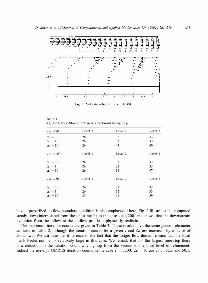
D. Silvester et al. / Journal of Computational and Applied Mathematics 128 (2001) 261–279 275
Fig. 2. Velocity solution for � = 1=200.
Table 3Nh
Mt for Navier–Stokes ,ow over a backward facing step
� = 1=50 Level 1 Level 2 Level 3
Mt = 0:1 26 32 33Mt = 1 26 32 33Mt = 10 26 43 40
� = 1=100 Level 1 Level 2 Level 3
Mt = 0:1 26 32 33Mt = 1 26 32 33Mt = 10 26 51 47
� = 1=200 Level 1 Level 2 Level 3
Mt = 0:1 26 32 33Mt = 1 26 32 33Mt = 10 33 64 59
have a prescribed out,ow boundary condition is also emphasized here. Fig. 2 illustrates the computedsteady ,ow (interpolated from the Jnest mesh) in the case �=1=200, and shows that the downstreamevolution from the in,ow to the out,ow proJle is physically realistic.
The maximum iteration counts are given in Table 3. These results have the same general characteras those in Table 2, although the iteration counts for a given � and Mt are increased by a factor ofabout two. We attribute this di:erence to the fact that the longer ,ow domain means that the localmesh PTeclet number is relatively large in this case. We remark that for the largest time-step thereis a reduction in the iteration count when going from the second to the third level of reJnement.Indeed the average GMRES iteration counts in the case �= 1=200; Mt = 10 are 27:3; 52:3 and 50.1,
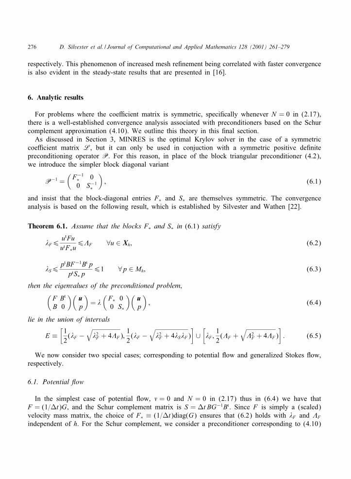
276 D. Silvester et al. / Journal of Computational and Applied Mathematics 128 (2001) 261–279
respectively. This phenomenon of increased mesh reJnement being correlated with faster convergenceis also evident in the steady-state results that are presented in [16].
6. Analytic results
For problems where the coe$cient matrix is symmetric, speciJcally whenever N = 0 in (2.17),there is a well-established convergence analysis associated with preconditioners based on the Schurcomplement approximation (4.10). We outline this theory in this Jnal section.
As discussed in Section 3, MINRES is the optimal Krylov solver in the case of a symmetriccoe$cient matrix L, but it can only be used in conjuction with a symmetric positive deJnitepreconditioning operator P. For this reason, in place of the block triangular preconditioner (4.2),we introduce the simpler block diagonal variant
P−1 =(F−1∗ 00 S−1
∗
); (6.1)
and insist that the block-diagonal entries F∗ and S∗ are themselves symmetric. The convergenceanalysis is based on the following result, which is established by Silvester and Wathen [22].
Theorem 6.1. Assume that the blocks F∗ and S∗ in (6:1) satisfy
.F6utFuutF∗u
63F ∀u ∈ Xh; (6.2)
.S6ptBF−1Btp
ptS∗p61 ∀p ∈ Mh; (6.3)
then the eigenvalues of the preconditioned problem;(F Bt
B 0
)(up
)= .
(F∗ 00 S∗
)(up
); (6.4)
lie in the union of intervals
E ≡[
12
(.F −√
.2F + 43F);
12
(.F −√
.2F + 4.S.F)
]∪[.F ;
12
(3F +√
32F + 43F)
]: (6.5)
We now consider two special cases; corresponding to potential ,ow and generalized Stokes ,ow,respectively.
6.1. Potential Bow
In the simplest case of potential ,ow, � = 0 and N = 0 in (2.17) thus in (6.4) we have thatF = (1=Mt)G, and the Schur complement matrix is S = Mt BG−1Bt . Since F is simply a (scaled)velocity mass matrix, the choice of F∗ ≡ (1=Mt)diag(G) ensures that (6.2) holds with .F and 3F
independent of h. For the Schur complement, we consider a preconditioner corresponding to (4.10)
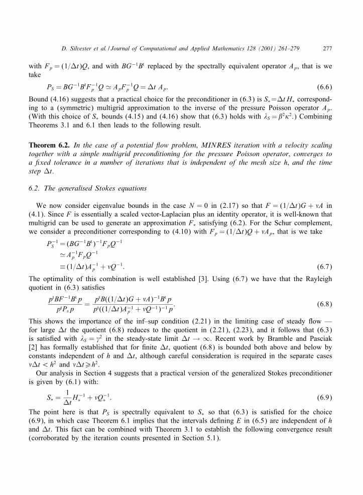
D. Silvester et al. / Journal of Computational and Applied Mathematics 128 (2001) 261–279 277
with Fp = (1=Mt)Q, and with BG−1Bt replaced by the spectrally equivalent operator Ap, that is wetake
PS = BG−1BtF−1p Q � ApF−1
p Q = Mt Ap: (6.6)
Bound (4.16) suggests that a practical choice for the preconditioner in (6.3) is S∗=Mt H∗ correspond-ing to a (symmetric) multigrid approximation to the inverse of the pressure Poisson operator Ap.(With this choice of S∗ bounds (4.15) and (4.16) show that (6.3) holds with .S =22�2.) CombiningTheorems 3.1 and 6.1 then leads to the following result.
Theorem 6.2. In the case of a potential Bow problem; MINRES iteration with a velocity scalingtogether with a simple multigrid preconditioning for the pressure Poisson operator; converges toa >xed tolerance in a number of iterations that is independent of the mesh size h; and the timestep Mt.
6.2. The generalised Stokes equations
We now consider eigenvalue bounds in the case N = 0 in (2.17) so that F = (1=Mt)G + �A in(4.1). Since F is essentially a scaled vector-Laplacian plus an identity operator, it is well-known thatmultigrid can be used to generate an approximation F∗ satisfying (6.2). For the Schur complement,we consider a preconditioner corresponding to (4.10) with Fp = (1=Mt)Q + �Ap, that is we take
P−1S = (BG−1Bt)−1FpQ−1
�A−1p FpQ−1
≡ (1=Mt)A−1p + �Q−1: (6.7)
The optimality of this combination is well established [3]. Using (6.7) we have that the Rayleighquotient in (6.3) satisJes
ptBF−1BtpptPsp
=ptB((1=Mt)G + �A)−1Btppt((1=Mt)A−1
p + �Q−1)−1p: (6.8)
This shows the importance of the inf–sup condition (2.21) in the limiting case of steady ,ow —for large Mt the quotient (6.8) reduces to the quotient in (2.21), (2.23), and it follows that (6.3)is satisJed with .S = �2 in the steady-state limit Mt → ∞. Recent work by Bramble and Pasciak[2] has formally established that for Jnite Mt, quotient (6.8) is bounded both above and below byconstants independent of h and Mt, although careful consideration is required in the separate cases�Mt ¡h2 and �Mt¿h2.
Our analysis in Section 4 suggests that a practical version of the generalized Stokes preconditioneris given by (6.1) with:
S∗ =1
MtH−1
∗ + �Q−1∗ : (6.9)
The point here is that PS is spectrally equivalent to S∗ so that (6.3) is satisJed for the choice(6.9), in which case Theorem 6.1 implies that the intervals deJning E in (6.5) are independent of hand Mt. This fact can be combined with Theorem 3.1 to establish the following convergence result(corroborated by the iteration counts presented in Section 5.1).
278 D. Silvester et al. / Journal of Computational and Applied Mathematics 128 (2001) 261–279
Theorem 6.3. In the case of a generalized Stokes problem; preconditioned MINRES iteration witha simple multigrid cycle approximating a Helmholtz operator for each velocity component and aPoisson operator for the pressure; converges to a >xed tolerance in a number of iterations that isindependent of the mesh size h; and the time step Mt.
7. Conclusion
The Navier–Stokes solution algorithm that is outlined in this work is rapidly converging, and theresulting iteration counts are remarkably insensitive to the mesh size and time-step. The algorithm isalso robust with respect to variations in the Reynolds number of the underlying ,ow. An attractivefeature of our approach is that it can be implemented using simple building blocks for solving thetwo subsidiary problems that arise, namely, a pressure Poisson problem and a scalar convection–di:usion problem. If multigrid is used for each of these then the overall complexity is proportionalto the number of degrees of freedom.
Acknowledgements
This is ongoing research and is supported by the EPSRC via grants GR=K91262 (DS), GR/M59044(AW) and GR=L05617 (DK) and by the US National Science Foundation via grant DMS9972490.
References
[1] M. Bercovier, O.A. Pironneau, Error estimates for Jnite element method solution of the Stokes problem in theprimitive variables, Numer. Math. 33 (1977) 211–224.
[2] J. Bramble, J. Pasciak, Iterative techniques for time dependent Stokes problems, Math. Appl. 33 (1997) 13–30.[3] J. Cahouet, J.P. Chabard, Some fast 3D Jnite element solvers for the generalised Stokes problem, Internat. J. Numer.
Methods Fluids 8 (1988) 869–895.[4] S.C. Eisenstat, H.C. Elman, M.H. Schultz, Variational iterative methods for nonsymmetric systems of linear equations,
SIAM J. Numer. Anal. 20 (1983) 345–357.[5] H. Elman, Preconditioning for the steady state Navier–Stokes equations with low viscosity, SIAM J. Sci. Comput.
20 (1999) 1299–1316.[6] H. Elman, D. Silvester, Fast nonsymmetric iterations and preconditioning for Navier–Stokes equations, SIAM J. Sci.
Comput. 17 (1996) 33–46.[7] H.C. Elman, D.J Silvester, A.J. Wathen, Performance and analysis of saddle point preconditioners for the discrete
steady-state Navier–Stokes equations, Technical Report UMIACS-TR-2000-54 (2000).[8] V. Faber, T.A. Manteu:el, Necessary and su$cient conditions for the existence of a conjugate gradient method,
SIAM J. Numer. Anal. 21 (1984) 352–362.[9] V. Faber, T.A. Manteu:el, Orthogonal error methods, SIAM J. Numer. Anal. 24 (1987) 170–187.
[10] B. Fischer, A. Ramage, D. Silvester, A. Wathen, On parameter choice and iterative convergence for stabiliseddiscretisations of advection-di:usion problems, Comput. Methods Appl. Mech. Eng. 179 (1999) 185–202.
[11] R. Freund, N.M. Nachtigal, QMR: a quasi-minimal residual method for non-Hermitian linear systems, Numer. Math.60 (1991) 315–339.
[12] R. Freund, N.M. Nachtigal, A new Krylov-subspace method for symmetric indeJnite linear systems, in: Ames, W.F.(Ed.), Proceedings of the 14th IMACS World Congress on Computational and Applied Mathematics, IMACS, 1994,pp. 1253–1256.
D. Silvester et al. / Journal of Computational and Applied Mathematics 128 (2001) 261–279 279
[13] V. Girault, P.A. Raviart, Finite Element Methods for Navier–Stokes Equations—Theory and Algorithms, Springer,Berlin, 1986.
[14] P.M. Gresho, R. Sani, Incompressible Flow and the Finite Element Method, Wiley, Chichester, 1998.[15] C. Johnson, The streamline di:usion Jnite element method for compressible and incompressible ,ow, in: D.F.
Gri$ths, G.A. Watson (Eds.), Numerical Analysis 1989, Longman ScientiJc, 1989, pp. 155–181.[16] D. Kay, D. Loghin, A Green’s function preconditioner for the steady state Navier–Stokes equations, Oxford University
Computing Laboratory Report 99=06, 1999, SIAM J. Sci. Comput., submitted for publication.[17] D. Kay, D. Silvester, A posteriori error estimation for stabilised mixed approximations of the Stokes equations,
SIAM J. Sci. Comput. 21 (2000) 1321–1336.[18] V.I. Lebedev, Iterative methods for solving operator equations with a spectrum contained in several intervals, USSR
Comput. Math. and Math. Phys. 9 (1969) 17–24.[19] M.F. Murphy, G.H. Golub, A.J. Wathen, A note on preconditioning for indeJnite linear systems, SIAM J. Sci.
Comput. 21 (2000) 1969–1972.[20] C.C. Paige, M.A. Saunders, Solution of sparse indeJnite systems of linear equations, SIAM. J. Numer. Anal. 12
(1975) 617–629.[21] Y. Saad, M.H. Schultz, GMRES: a generalized minimal residual algorithm for solving nonsymmetric linear systems,
SIAM J. Sci. Statist. Comput. 7 (1986) 856–869.[22] D. Silvester, A. Wathen, Fast iterative solution of stabilised Stokes systems part II: using general block
preconditioners, SIAM J. Numer. Anal. 31 (1994) 1352–1367.[23] D. Silvester, A. Wathen, Fast & robust solvers for time-discretised incompressible Navier–Stokes equations, in: D.F.
Gri$ths, G.A. Watson (Eds.), Numerical Analysis 1995, Longman ScientiJc, 1996, pp. 230–240.[24] J. Simo, F. Armero, Unconditional stability and long-term behavior of transient algorithms for the incompressible
Navier–Stokes and Euler equations, Comput. Methods Appl. Mech. Eng. 111 (1994) 111–154.[25] G.L.G. Sleijpen, D.R. Fokkema, BiCGSTAB(‘) for linear equations involving unsymmetric matrices with complex
spectrum, Electron. Trans. Numer. Anal. 1 (1993) 11–32.[26] A. Smith, D. Silvester, Implicit algorithms and their linearisation for the transient Navier–Stokes equations, IMA J.
Numer. Anal. 17 (1997) 527–543.[27] P. Sonneveld, CGS, a fast Lanczos-type solver for nonsymmetric linear systems, SIAM J. Sci. Statist. Comput. 10
(1989) 36–52.[28] G. Stoyan, Towards discrete Velte decompositions and narrow bounds for inf-sup constants, Comput. Math. Appl.
38 (1999) 243–261.[29] S. Turek, E$cient Solvers for Incompressible Flow Problems, Springer, Berlin, 1999.[30] H.A. Van der Vorst, BI-CGSTAB: a fast and smoothly converging variant of BI-CG for the solution of nonsymmetric
linear systems, SIAM J. Sci. Statist. Comput. 10 (1992) 631–644.[31] A.J. Wathen, Realistic eigenvalue bounds for the Galerkin mass matrix, IMA J. Numer. Anal. 7 (1987) 449–457.[32] A. Wathen, B. Fischer, D. Silvester, The convergence rate of the minimal residual method for the Stokes problem,
Numer. Math. 71 (1995) 121–134.[33] A. Wathen, B. Fischer, D. Silvester, The convergence of iterative solution methods for symmetric and indeJnite
linear systems, in: D.F. Gri$ths, D.J. Higham, G.A. Watson (Eds.), Numerical Analysis 1997, Longman ScientiJc,1997, pp. 230–243.
[34] P. Wesseling, An Introduction to Multigrid, Wiley, New York, 1991.

Journal of Computational and Applied Mathematics 128 (2001) 281–309www.elsevier.nl/locate/cam
A review of algebraic multigridK. St&uben
German National Research Center for Information Technology (GMD), Institute for Algorithms and Scienti�cComputing (SCAI), Schloss Birlinghoven, D-53754 St. Augustin, Germany
Received 3 September 1999; received in revised form 9 November 1999
Abstract
Since the early 1990s, there has been a strongly increasing demand for more e,cient methods to solve large sparse,unstructured linear systems of equations. For practically relevant problem sizes, classical one-level methods had alreadyreached their limits and new hierarchical algorithms had to be developed in order to allow an e,cient solution of evenlarger problems. This paper gives a review of the 1rst hierarchical and purely matrix-based approach, algebraic multigrid(AMG). AMG can directly be applied, for instance, to e,ciently solve various types of elliptic partial di3erential equationsdiscretized on unstructured meshes, both in 2D and 3D. Since AMG does not make use of any geometric information,it is a “plug-in” solver which can even be applied to problems without any geometric background, provided that theunderlying matrix has certain properties. c© 2001 Elsevier Science B.V. All rights reserved.
Keywords: Algebraic multigrid
1. Introduction
The e,cient numerical solution of large systems of discretized elliptic partial di3erential equations(PDEs) requires hierarchical algorithms which ensure a rapid reduction of both short- and long-rangeerror components. A break-through, and certainly one of the most important advances during the lastthree decades, was due to the multigrid principle. Any corresponding method operates on a hierarchyof grids, de1ned a priori by coarsening the given discretization grid in a geometrically natural way(“geometric” multigrid). Clearly, this is straightforward for logically regular grids. However, thede1nition of a natural hierarchy may become very complicated for highly complex, unstructuredmeshes, if possible at all.
The 1rst attempt to automate the coarsening process took place in the early 1980s [10,12,13],at the time when the so-called Galerkin-principle and operator-dependent interpolation were com-bined in geometric multigrid to increase its robustness (aiming at the e,cient solution of di3usion
E-mail address: [email protected] (K. St&uben).
0377-0427/01/$ - see front matter c© 2001 Elsevier Science B.V. All rights reserved.PII: S 0377-0427(00)00516-1
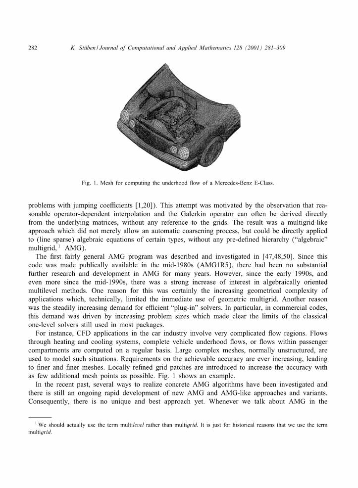
282 K. St0uben / Journal of Computational and Applied Mathematics 128 (2001) 281–309
Fig. 1. Mesh for computing the underhood Iow of a Mercedes-Benz E-Class.
problems with jumping coe,cients [1,20]). This attempt was motivated by the observation that rea-sonable operator-dependent interpolation and the Galerkin operator can often be derived directlyfrom the underlying matrices, without any reference to the grids. The result was a multigrid-likeapproach which did not merely allow an automatic coarsening process, but could be directly appliedto (line sparse) algebraic equations of certain types, without any pre-de1ned hierarchy (“algebraic”multigrid, 1 AMG).The 1rst fairly general AMG program was described and investigated in [47,48,50]. Since this
code was made publically available in the mid-1980s (AMG1R5), there had been no substantialfurther research and development in AMG for many years. However, since the early 1990s, andeven more since the mid-1990s, there was a strong increase of interest in algebraically orientedmultilevel methods. One reason for this was certainly the increasing geometrical complexity ofapplications which, technically, limited the immediate use of geometric multigrid. Another reasonwas the steadily increasing demand for e,cient “plug-in” solvers. In particular, in commercial codes,this demand was driven by increasing problem sizes which made clear the limits of the classicalone-level solvers still used in most packages.
For instance, CFD applications in the car industry involve very complicated Iow regions. Flowsthrough heating and cooling systems, complete vehicle underhood Iows, or Iows within passengercompartments are computed on a regular basis. Large complex meshes, normally unstructured, areused to model such situations. Requirements on the achievable accuracy are ever increasing, leadingto 1ner and 1ner meshes. Locally re1ned grid patches are introduced to increase the accuracy withas few additional mesh points as possible. Fig. 1 shows an example.
In the recent past, several ways to realize concrete AMG algorithms have been investigated andthere is still an ongoing rapid development of new AMG and AMG-like approaches and variants.Consequently, there is no unique and best approach yet. Whenever we talk about AMG in the
1 We should actually use the term multilevel rather than multigrid. It is just for historical reasons that we use the termmultigrid.

K. St0uben / Journal of Computational and Applied Mathematics 128 (2001) 281–309 283
context of concrete numerical results, we actually refer to the code RAMG05 2 (described in detailin [51]), which is a successor of the original code AMG1R5 mentioned above. However, RAMG05is completely new and, in particular, incorporates more e,cient and more robust interpolation andcoarsening strategies.
This paper gives a survey of the classical AMG idea [48], certain improvements and extensionsthereof, and various new approaches. The focus in Sections 2–6 is on fundamental ideas and aspects,targeting classes of problems for which AMG is best-developed, namely, symmetric positive-de�nite(s.p.d.) problems of the type as they arise, for instance, from the discretization of scalar elliptic PDEsof second order. We want to point out, however, that the potential range of applicability is muchlarger. In particular, AMG has successfully been applied to various nonsymmetric (e.g. convection–di3usion) and certain inde1nite problems. Moreover, important progress has been achieved in thenumerical treatment of systems of PDEs (mainly Navier–Stokes and structural mechanics applica-tions). However, major research is still ongoing and much remains to be done to obtain an e,ciencyand robustness comparable to the case of scalar applications. In particular in Section 7, we will setpointers to the relevant literature where one can 1nd further information or more recent AMG ap-proaches. Although we try to cover the most important references, the list is certainly not completein this rapidly developing 1eld of research.
2. Algebraic versus geometric multigrid
Throughout this paper, we assume the reader to have some basic knowledge of geometric multi-grid. In particular, he should be familar with the fundamental principles (smoothing and coarse-gridcorrection) and with the recursive de1nition of multigrid cycles. This is because, for simplicity, welimit our main considerations to just two levels. Accordingly, whenever we talk about the e,ciencyof a particular approach, we implicitly always assume the underlying two-level method to be recur-sively extended to a real multi-level method, involving only a small number of variables (20–40,say) on the coarsest level. Regarding more detailed information on geometric multigrid, we refer to[61] and the extensive list of references given therein.
A two-level AMG cycle to solve (sparse) s.p.d. systems of equations
Ahuh =fh or∑
j∈�h
ahiju
hj =fh
i (i∈�h) (1)
is formally de1ned in the same way as a Galerkin-based geometric two-grid cycle. The only di3erenceis that, in the context of AMG, �h is just an index set while it corresponds to a grid in geometricmultigrid. Accordingly, a coarser level, �H , just corresponds to a (much smaller) index set.
If we know how to map H -vectors into h-vectors by some (full rank) “interpolation” operator I hH ,
the (s.p.d.) coarse-level operator AH is de1ned via
AH := I Hh AhI h
H with I Hh =(I h
H)T:
One two-level correction step then runs as usual, that is
uhnew = uh
old + I hHe
H ; (2)
2 The development of RAMG05 has partly been funded by Computational Dynamics Ltd., London.
284 K. St0uben / Journal of Computational and Applied Mathematics 128 (2001) 281–309
where the correction eH is the exact solution of
AHeH = r H or∑
j∈�HaHij e
Hj = r H
i (i∈�H)
with r H = I Hh (r h
old) and r hold =fh−Ahuh
old. (Note that we normally use the letter u for solution quantitiesand the letter e for correction or error quantities.) For the corresponding errors eh = uh
? − uh (uh?
denotes the exact solution of (1)), this means
ehnew =Kh;Heh
old with Kh;H := Ih − I hHA
−1H I H
h Ah; (3)
being the coarse-grid correction operator (Ih denotes the identity).We 1nally recall that – given any relaxation operator, Sh, for smoothing – the convergence
of Galerkin-based approaches can most easily be investigated w.r.t. the energy norm, ‖eh‖Ah=
(Aheh; e h)1=2. Assuming � relaxation steps to be performed for (pre-) smoothing, the followingwell-known variational principle holds (see, for instance [51]),
‖Kh;HS�he
h‖Ah= min
e H‖S�
heh − I h
HeH‖Ah
: (4)
As a trivial consequence, convergence of two-level cycles and, if recursively extended to anynumber of levels, the convergence of complete V-cycles is always ensured as soon as the relax-ation method converges. This is true for any sequence of coarser levels and interpolation operators.More importantly, (4) indicates that the speed of convergence strongly depends on the e,cient in-terplay between relaxation and interpolation. Based on (4), we want to outline the basic conceptualdi3erence between geometric and algebraic multigrid.
2.1. Geometric multigrid
In geometric multigrid, 1xed coarsening strategies are employed and interpolation is usually de1nedgeometrically, typically by linear interpolation. Depending on the given problem, this necessarilyimposes strong requirements on the smoothing properties of Sh (in order for the right-hand side in(4) to become small), namely, that the error after relaxation varies in a geometrically smooth wayfrom the 1ne-level grid points to the neighboring coarse-level ones. In other words, the error afterrelaxation has to be geometrically smooth, relative to the coarse grid.
As an illustration, let us assume the coarser levels to be de1ned by standard geometric h→ 2hcoarsening in each spatial direction. It is well known that pointwise relaxation geometrically smoothsthe error in each direction only if the given problem is essentially isotropic. In case of anisotropicproblems, however, smoothing is only “in the direction of strong couplings”. In such cases, morecomplex smoothers, such as alternating line-relaxation or ILU-type schemes, are required in or-der to still achieve a good interplay between smoothing and interpolation and, thus, fast multigridconvergence.
While the construction of “robust smoothers” is not di,cult in 2D model situations, for 3D ap-plications on complex meshes their realization tends to become rather cumbersome. For instance,the robust 3D analog of alternating line relaxation is alternating plane relaxation (e.g., realized by2D multigrid within each plane) which, in complex geometric situations, becomes very complicatedto implement, if possible at all. ILU smoothers, on the other hand, loose much of their smoothingproperty in general 3D situations. The only way to loosen the requirements on the smoothing prop-erties of the relaxation and still maintain an e,cient interplay relaxation and interpolation is to use

K. St0uben / Journal of Computational and Applied Mathematics 128 (2001) 281–309 285
more sophisticated coarsening techniques. In geometric multigrid, steps in this direction have beendone by, for example, employing more than one coarser grid on each multigrid level (“multiplesemi-coarsening” [35,59,21,34]).
2.2. Algebraic multigrid
While geometric multigrid essentially relies on the availability of robust smoothers, AMG takesthe opposite point of view. It assumes a simple relaxation process to be given (typically plainGauss–Seidel relaxation) and then attempts to construct a suitable operator-dependent interpolationI hH (including the coarser level itself). According to (4), this construction has to be such that errorof the form S�
heh is su,ciently well represented in the range of interpolation, R(I h
H). The better thisis satis1ed, the faster the convergence can be. Note that it is not important here whether relaxationsmooths the error in any geometric sense. What is important, though, is that the error after relaxationcan be characterized algebraically to a degree which makes it possible to automatically constructcoarser levels and de1ne interpolations which are locally adapted to the properties of the givenrelaxation. This local adaptation is the main reason for AMG’s Iexibility in adjusting itself to theproblem at hand and its robustness in solving large classes of problems despite using very simplepoint-wise smoothers.
3. The classical AMG approach
In classical AMG, we regard the coarse-level variables as a subset of the 1ne-level ones. Thatis, we assume the set of 1ne-level variables to be split into two disjoint subsets, �h =C h ∪ F h,with C h representing those variables which are to be contained in the coarse level (C-variables) andF h being the complementary set (F-variables). Given such a C=F-splitting, we de1ne �H =C h andconsider (full rank) interpolations eh = I h
HeH of the form
ehi =(I h
HeH)i =
eHi if i∈C h;∑k ∈ P h
iw h
ikeHk if i∈F h;
(5)
where Phi ⊂C h is called the set of interpolatory variables. (For reasons of sparsity of AH , Ph
i shouldbe a reasonably small subset of C-variables “near” i.) Clearly, R(I h
H) strongly depends on both theconcrete selection of the C-variables and the de1nition of the interpolation. In a given situation,one can easily imagine “bad” C=F-splittings which just do not allow any interpolation which issuitable in the sense that was outlined in the previous section. That is, the construction of concreteC=F-splittings and the de1nition of interpolation are closely related processes.
Concrete algorithms used in practice are largely heuristically motivated. In Section 3.1, we mainlysummarize the basic ideas as described in [48] and some modi1cations introduced in [51]. In Section3.2, we take a closer look at some theoretical and practical aspects in case that Ah contains onlynonpositive o3-diagonal entries (M -matrix). To simplify notation, we usually omit the index h in thefollowing, for instance, we write S; A; K and e instead of Sh; Ah; Kh;H and eh. Moreover, insteadof (5), we simply write
ei =∑k ∈ Pi
wikek (i∈F): (6)

286 K. St0uben / Journal of Computational and Applied Mathematics 128 (2001) 281–309
3.1. The basic ideas
Classical AMG uses plain Gauss–Seidel relaxation for smoothing. From some heuristic arguments,one can see that the error e, obtained after a few relaxation steps, is characterized by the fact thatthe (scaled) residual is, on the average for each i, much smaller than the error itself, |ri|�aii|ei|.This implies that ei can locally be well approximated by
ei ≈ −∑
j∈Ni
aijej
/ aii (i∈�); (7)
where Ni = {j∈�: j �= i; aij �=0} denotes the neighborhood of any i∈�. Such an error is calledalgebraically smooth. According to the remarks at the end of Section 2, it is this kind of errorwhich has to be well represented in R(I h
H). That is, the general goal is to construct C=F-splittingsand de1ne sets of interpolatory variables Pi⊂C (i∈F) along with corresponding weights wik suchthat (6) yields a reasonable approximation for each algebraically smooth vector e.
Obviously, a very “accurate” interpolation in this sense is obtained by directly using (7), thatis, by choosing Pi =Ni and wik = − aik=aii. However, this would require selecting a C=F-splittingso that, for each i∈F , all of its neighbors are contained in C. Although any such selection caneven be seen to yield a direct solver, this approach is of no real practical relevance since, in termsof computational work and memory requirement, the resulting method will generally be extremelyine,cient if recursively extended to a hierarchy of levels [51].
In practice, we want to achieve rapid convergence with as small sets of interpolatory variablesPi as possible (in order to allow for a rapid coarsening and to obtain reasonably sparse Galerkinoperators). Various approaches have been tested in practice which cannot be described in detail here.In the following, we just give an outline of some typical approaches.
3.1.1. Direct interpolationWe talk about direct interpolation if Pi⊆Ni. Such an interpolation can immediately be derived
from (7) if we know how to approximate the “noninterpolatory part” (i.e. that part of the sum in(7) which refers to j∈Ni \ Pi) for an algebraically smooth error. This approximation is the mostcritical step in de1ning interpolation.
For M -matrices A, for instance, such an approximation can be obtained by observing that analgebraically smooth error varies slowly in the direction of strong (large) couplings. In particular,the more strong couplings of any variable i are contained in Pi, the better an algebraically smootherror satis1es
1∑k ∈ Pi
aik
∑k ∈ Pi
aikek ≈ 1∑j∈Ni
aij
∑j∈Ni
aijej (i∈�):
Inserting this into (7), we obtain an interpolation (6) with positive weights
wik = − �iaik=aii where �i =
∑j∈Ni
aij∑‘∈ Pi
ai‘: (8)
Practically, this means that we have to construct C=F-splittings so that each i∈F has a su,cientlylarge number of strongly coupled C-neighbors which are then taken as the set of interpolatoryvariables Pi. (See Section 3.2 regarding some important additional aspects.)

K. St0uben / Journal of Computational and Applied Mathematics 128 (2001) 281–309 287
In the case of (scalar) elliptic PDEs, the largest o3-diagonal entries are usually negative. If thereare also positive o3-diagonal entries, a similar process as before can be applied as long as such entriesare relatively small: Small positive couplings can simply be ignored by just considering them asweak. However, the situation becomes less obvious, if A contains large positive o3-diagonal entries.In many such cases, an algebraically smooth error can be assumed to oscillate along such couplings(e.g. in case of weakly diagonally dominant s.p.d. matrices A [26,51]). This can be used to generalizethe above approach by, for instance, a suitable separation of positive and negative couplings, leadingto interpolation formulas containing both positive and negative weights. A corresponding approachhas been proposed in [51] which can formally be applied to arbitrary s.p.d. matrices. However, theresulting interpolation is heuristically justi1ed only as long as, for any i, those error components ekwhich correspond to large positive couplings aik ¿ 0, change slowly among each other (unless aik
is very small in which case its inIuence can be ignored).In practice, these simple algebraic approaches to construct an interpolation cover a large class of
applications. However, there is no best way yet to automatically construct an interpolation which isgood for arbitrary s.p.d. matrices, at least not by merely considering the size and sign of coe,cients.For instance, in case of particular higher-order 1nite-element discretizations or discretizations bybilinear elements on quadrilateral meshes with large aspect ratios, the resulting matrices typicallycontain signi1cant positive o3-diagonal entries and are far from being weakly diagonally dominant.In such cases, the performance of AMG may be only suboptimal. If this happens, it often helps toexploit some information about the origin of these positive connections rather than to rely only oninformation directly contained in the matrix. For instance, one could try to structurally simplify thegiven matrix before applying AMG (see, e.g. [41]). Alternative approaches, de1ning the coarseningand interpolation are outlined in Section 7.
3.1.2. More complex interpolationsThere are several ways to improve the direct interpolation of the previous section. To outline some
possibilities, let us assume a C=F-splitting and, for each i∈F , a set of (strongly coupled) interpola-tory variables Pi⊆Ni ∩C to be given. Rather than to immediately approximate the noninterpolatorypart of the ith equation (7) as done above, one may 1rst (approximately) eliminate all stronglycoupled ej (j =∈Pi) by means of the corresponding jth equation. The ideas outlined in the previoussection can then analogously be applied to the resulting extended equation for ei, leading to aninterpolation with an increased set of interpolatory variables. The corresponding interpolation (calledstandard interpolation in [51]) is, in general, considerably more robust in practice. Alternatively,one may obtain an improved interpolation by applying one F-relaxation step (for more details, see“Jacobi-interpolation” in Section 5) to either the direct or the standard interpolation.
In both approaches, compared to the direct interpolation, the “radius” of interpolation increaseswhich, in turn, will reduce the sparsity of the resulting Galerkin operator. However, interpolationweights corresponding to variables “far away” from variable i are typically much smaller than thelargest ones. Before computing the Galerkin operator, one should therefore truncate the interpolationoperator by ignoring all small entries (and re-scale the remaining weights so that the total sumremains unchanged). Note that, because of the variational principle, the truncation of interpolationis a “safe process”; in the worst case, overall convergence may slow down, but no divergence canoccur. On the other hand, a truncation of the Galerkin operators can be dangerous since this destroys
288 K. St0uben / Journal of Computational and Applied Mathematics 128 (2001) 281–309
the validity of the variational principle and, if not applied with great care, may even cause strongdivergence in practice.
Apart from other minor di3erences, the original AMG interpolation proposed in [48] (and realizedin the code AMG1R5) can be regarded as a compromise between the direct interpolation and thestandard interpolation described before. There, an attempt was made to replace all strongly coupledej (j =∈Pi) in (7) by averages involving only variables in Pi. However, for this to be reasonable,based on certain criteria, new C-variables had to be added to a given splitting a posteriori (“1nalC-point choice” in [48]). Although this approach worked quite well in those cases treated in [48],typically too many additional C-variables are required in geometrically complex 3D situations, caus-ing unacceptably high 1ll-in towards coarser levels (see Section 4.2 for examples). In practice, thestandard interpolation outlined above (in combination with a reasonable truncation) has turned outto be more robust and often considerably more e,cient.
The above improvements of interpolation generally lead to faster convergence but also increasethe computational work per cycle and the required memory to some extent. Whether or not this1nally pays, depends on the given application. If memory is an issue (as it is often in commer-cial environments), one may, instead, wish to simplify interpolation at the expense of a reducedconvergence speed. One way to achieve this is to generally allow interpolation from variableswhich are not in the direct neighborhood. Such “long-range” interpolation [48] generally allowsa much faster coarsening and drastically increases the sparsity on coarser levels. For details of asimple approach which has been tested in practice, see [51] (“aggressive coarsening” and “multi-passinterpolation”).
3.2. The M-matrix case
In practice, it turns out that AMG V-cycle convergence is, to a large extent, independent of theproblem size. Unfortunately, this cannot be proved based merely on algebraic arguments. Never-theless, some important aspects can be investigated theoretically, in particular, matrix-independenttwo-level convergence can be proved for various classes of matrices if interpolation is de1ned prop-erly. We consider here the class of M -matrices. Generalizations to other classes and the correspondingproofs can be found in [51].
3.2.1. Two-level considerationsThe following theorem shows that direct interpolation based on (8) ensures matrix-independent
two-level convergence if, for each i∈F , the connectivity represented in Pi is a �xed fraction of thetotal connectivity.
Theorem 1. Let A be a symmetric; weakly diagonally dominant M -matrix. With �xed 0¡�61select a C=F-splitting so that; for each i∈F; there is a set Pi⊆C ∩ Ni satisfying∑
k ∈ Pi
|aik |¿�∑j∈Ni
|aij| (9)
and de�ne interpolation according to (8). Then the two-level method; using one Gauss–Seidelrelaxation step for ( post-) smoothing; converges at a rate which depends only on � but not on the
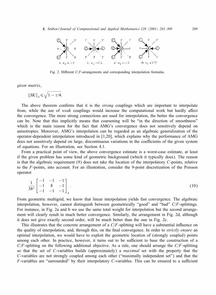
K. St0uben / Journal of Computational and Applied Mathematics 128 (2001) 281–309 289
Fig. 2. Di3erent C=F-arrangements and corresponding interpolation formulas.
given matrix;
‖SK‖A6√1− �=4:
The above theorem con1rms that it is the strong couplings which are important to interpolatefrom, while the use of weak couplings would increase the computational work but hardly a3ectthe convergence. The more strong connections are used for interpolation, the better the convergencecan be. Note that this implicitly means that coarsening will be “in the direction of smoothness”which is the main reason for the fact that AMG’s convergence does not sensitively depend onanisotropies. Moreover, AMG’s interpolation can be regarded as an algebraic generalization of theoperator-dependent interpolation introduced in [1,20], which explains why the performance of AMGdoes not sensitively depend on large, discontinuous variations in the coe,cients of the given systemof equations. For an illustration, see Section 4.1.
From a practical point of view, the above convergence estimate is a worst-case estimate, at leastif the given problem has some kind of geometric background (which it typically does). The reasonis that the algebraic requirement (9) does not take the location of the interpolatory C-points, relativeto the F-points, into account. For an illustration, consider the 9-point discretization of the Poissonoperator
13h2
−1 −1 −1−1 8 −1−1 −1 −1
h
: (10)
From geometric multigrid, we know that linear interpolation yields fast convergence. The algebraicinterpolation, however, cannot distinguish between geometrically “good” and “bad” C=F-splittings.For instance, in Fig. 2a and b we use the same total weight for interpolation but the second arrange-ment will clearly result in much better convergence. Similarly, the arrangement in Fig. 2d, althoughit does not give exactly second order, will be much better than the one in Fig. 2c.
This illustrates that the concrete arrangement of a C=F-splitting will have a substantial inIuence onthe quality of interpolation, and, through this, on the 1nal convergence. In order to strictly ensure anoptimal interpolation, we would have to exploit the geometric location of (strongly coupled) pointsamong each other. In practice, however, it turns out to be su,cient to base the construction of aC=F-splitting on the following additional objective. As a rule, one should arrange the C=F-splittingso that the set of C-variables builds (approximately) a maximal set with the property that theC-variables are not strongly coupled among each other (“maximally independent set”) and that theF-variables are “surrounded” by their interpolatory C-variables. This can be ensured to a su,cient
290 K. St0uben / Journal of Computational and Applied Mathematics 128 (2001) 281–309
extent by merely exploiting the connectivity information contained in the matrix (for an algorithm,see [48,51]). Note that strong connectivity does not necessarily have to be via direct couplings.
Observing this objective will, in practice, substantially enhance convergence even if only smallsets of interpolatory variables are used.
3.2.2. Extension to multi-level cyclesUnfortunately, the assumptions on interpolation in Theorem 1 are su,cient for uniform two-level,
but not for uniform V-cycle convergence. Although, by choosing �¿ 12 , one can ensure that all
recursively de1ned Galerkin operators remain weakly diagonally dominant M -matrices and, hence,the formal extension to complete V-cycles is straightforward, A-independent V-cycle convergencecannot be proved. The reason is the limited accuracy of purely algebraically de1ned interpolation asdiscussed in the previous section. We will return to this problem in Section 6 where we consider aworst-case scenario in the context of “aggregation-type” AMG approaches.
In practice, however, one can observe V-cycle convergence which is, to a large extent, indepen-dent of the problem size if we take the additional objective of the previous section into account.Furthermore, it turns out that it is not important to force the coarse-level matrices to exactly re-main M -matrices. On the contrary, such a requirement puts too many restrictions on the coarseningprocess, in particular on lower levels, where the size of the Galerkin operators then may growsubstantially.
In this context, we want to emphasize again that, for an e,cient overall performance, convergencespeed is only one aspect. An equally important aspect is the complexity (sparsity) of the coarser levelmatrices produced by AMG (which directly inIuences both the run time and the overall memoryrequirement). Only if both the convergence speed and the operator complexity
cA =∑l
|ml|=|m1|; (11)
(ml denotes the number of nonzero entries contained in the matrix on level ‘) are bounded inde-pendent of the size of A, do we have an asymptotically optimal performance. The typical AMGperformance in case of some complex problems is given in Section 4.2.
3.3. AMG as a pre-conditioner
In order to increase the robustness of geometric multigrid approaches, it has become very popularduring the last years, to use multigrid not as a stand-alone solver but rather combine it with accelera-tion methods such as conjugate gradient. BI-CGSTAB or GMRES. This development was driven bythe observation that it is often not only simpler but also more e,cient to use accelerated multigridapproaches rather than to try to optimize the interplay between the various multigrid components inorder to improve the convergence of stand-alone multigrid cycles.
This has turned out to be similar for AMG which, originally, was designed to be used stand-alone.Practical experience has clearly shown that AMG is also a very good pre-conditioner, much betterthan standard (one-level) ILU-type pre-conditioners, say. Heuristically, the major reason is due tothe fact that AMG, in contrast to any one-level pre-conditioner, aims at the e,cient reduction ofall error components, short range as well as long range. However, although AMG tries to captureall relevant inIuences by proper coarsening and interpolation, its interpolation will hardly ever be
K. St0uben / Journal of Computational and Applied Mathematics 128 (2001) 281–309 291
optimal. It may well happen that error reduction is signi1cantly less e,cient for some very speci1cerror components. This may cause a few eigenvalues of the AMG iteration matrix to be considerablycloser to 1 than all the rest. If this happens, AMG’s convergence factor is limited by the slowconvergence of just a few exceptional error components while the majority of the error componentsis reduced very quickly. Acceleration by, for instance, conjugate gradient typically eliminates theseparticular frequencies very e,ciently. The alternative, namely, to try to prevent such situations byputting more e3ort into the construction of interpolation, will generally be much more expensive.Even then, there is no 1nal guarantee that such situations can be avoided. (We note that this evenhappens with “robust” geometric multigrid methods.)
4. Applications and performance
The Iexibility of AMG and its simplicity of use, of course, have a price: A setup phase, in whichthe given problem is analyzed, the coarse levels are constructed and all operators are assembled,has to be concluded before the actual solution phase can start. This extra overhead is one reasonfor the fact that AMG is usually less e,cient than geometric multigrid approaches (if applied toproblems for which geometric multigrid can be applied e,ciently). Another reason is that AMG’scomponents can, generally, not be expected to be “optimal”. They are always constructed on thebasis of compromises between numerical work and overall e,ciency. Nevertheless, if applied tostandard elliptic test problems, the computational cost of AMG’s solution phase (ignoring the setupcost) is typically comparable to the solution cost of a robust geometric multigrid solver [47].
However, AMG should not be regarded as a competitor of geometric multigrid. The strengths ofAMG are its robustness, its applicability in complex geometric situations and its applicability to evensolve certain problems which are out of the reach of geometric multigrid, in particular, problemswith no geometric or continuous background at all. In such cases, AMG should be regarded as ane,cient alternative to standard numerical methods such as conjugate gradient accelerated by typical(one-level) pre-conditioners. We will show some concrete performance comparisons in Section 4.2.Before, however, we want to illustrate the Iexibility of AMG in adjusting its coarsening processlocally to the smoothing properties of relaxation by means of a simple but characteristic modelequation.
4.1. A model problem for illustration
We consider the model equation
− (aux)x − (buy)y + cuxy =f(x; y); (12)
de1ned on the unit square with Dirichlet boundary conditions. We assume a= b=1 everywhereexcept in the upper left quarter of the unit square (where b=103) and in the lower right quarter(where a=103). The coe,cient c is zero except for the upper right quarter where we set c=2.The resulting discrete system is isotropic in the lower left quarter of the unit square but stronglyanisotropic in the remaining quarters. Fig. 3a shows what a “smooth” error looks like on the 1nestlevel after having applied a few Gauss–Seidel point relaxation steps to the homogeneous problem,

292 K. St0uben / Journal of Computational and Applied Mathematics 128 (2001) 281–309
Fig. 3. (a) “Smooth” error in case of problem (12). (b) The 1nest and three consecutive levels created by the standardAMG coarsening algorithm.
starting with a random function. The di3erent anisotropies as well as the discontinuities across theinterface lines are clearly reIected in the picture.
It is heuristically clear that such an error can only be e3ectively reduced by means of a coarser gridif that grid is obtained by essentially coarsening in the directions in which the error really changessmoothly in the geometric sense and if interpolation treats the discontinuities correctly. Indeed, seeSection 3.2, this is exactly what AMG does. First, the operator-based interpolation ensures the correcttreatment of the discontinuities. Second, AMG coarsening is in the direction of strong connectivity,that is, in the direction of smoothness.
Fig. 3b depicts the 1nest and three consecutive grids created by using standard AMG coarseningand interpolation. The smallest dots mark grid points which are contained only on the 1nest grid,the squares mark those points which are also contained on the coarser levels (the bigger the square,the longer the corresponding grid point stays in the coarsening process). The picture shows thatcoarsening is uniform in the lower left quarter where the problem is isotropic. In the other quarters,AMG adjusts itself to the di3erent anisotropies by locally coarsening in the proper direction. Forinstance, in the lower right quarter, coarsening is in the x-direction only. Since AMG takes onlystrong connections in coarsening into account and since all connections in the y-direction are weak,the individual lines are coarsened independently of each other. Consequently, the coarsening ofneighboring x-lines is not “synchronized”; it is actually a matter of “coincidence” where coarseningstarts within each line. This has to be observed in interpreting the coarsening pattern in the upperright quarter: within each diagonal line, coarsening is essentially in the direction of this line.
4.2. Complex applications
For a demonstration of AMG’s e,ciency, we consider some complex problems of the type typ-ically solved in two commercial codes designed for oil reservoir simulation and for computational;uid dynamics, respectively. In both codes, the numerical kernel requires the fast solution of scalarelliptic equations. While, in oil reservoir simulation, geometries are typically fairly simple but theunderlying problems have strongly anisotropic and discontinuous coe,cients (jumps by several or-ders of magnitude in a nearly random way), in computational Iuid dynamics these problems are
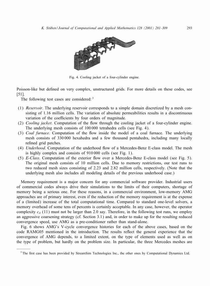
K. St0uben / Journal of Computational and Applied Mathematics 128 (2001) 281–309 293
Fig. 4. Cooling jacket of a four-cylinder engine.
Poisson-like but de1ned on very complex, unstructured grids. For more details on these codes, see[51].
The following test cases are considered: 3
(1) Reservoir. The underlying reservoir corresponds to a simple domain discretized by a mesh con-sisting of 1.16 million cells. The variation of absolute permeabilities results in a discontinuousvariation of the coe,cients by four orders of magnitude.
(2) Cooling jacket. Computation of the Iow through the cooling jacket of a four-cylinder engine.The underlying mesh consists of 100 000 tetrahedra cells (see Fig. 4).
(3) Coal furnace. Computation of the Iow inside the model of a coal furnace. The underlyingmesh consists of 330 000 hexahedra and a few thousand pentahedra, including many locallyre1ned grid patches.
(4) Underhood. Computation of the underhood Iow of a Mercedes-Benz E-class model. The meshis highly complex and consists of 910 000 cells (see Fig. 1).
(5) E-Class. Computation of the exterior Iow over a Mercedes-Benz E-class model (see Fig. 5).The original mesh consists of 10 million cells. Due to memory restrictions, our test runs totwo reduced mesh sizes consisting of 2.23 and 2.82 million cells, respectively. (Note that theunderlying mesh also includes all modeling details of the previous underhood case.)
Memory requirement is a major concern for any commercial software provider. Industrial usersof commercial codes always drive their simulations to the limits of their computers, shortage ofmemory being a serious one. For these reasons, in a commercial environment, low-memory AMGapproaches are of primary interest, even if the reduction of the memory requirement is at the expenseof a (limited) increase of the total computational time. Compared to standard one-level solvers, amemory overhead of some tens of percents is certainly acceptable. In any case, however, the operatorcomplexity cA (11) must not be larger than 2.0 say. Therefore, in the following test runs, we employan aggressive coarsening strategy (cf. Section 3.1) and, in order to make up for the resulting reducedconvergence speed, use AMG as a pre-conditioner rather than stand-alone.
Fig. 6 shows AMG’s V-cycle convergence histories for each of the above cases, based on thecode RAMG05 mentioned in the introduction. The results reIect the general experience that theconvergence of AMG depends, to a limited extent, on the type of elements used as well as onthe type of problem, but hardly on the problem size. In particular, the three Mercedes meshes are
3 The 1rst case has been provided by StreamSim Technologies Inc., the other ones by Computational Dynamics Ltd.

294 K. St0uben / Journal of Computational and Applied Mathematics 128 (2001) 281–309
Fig. 5. Model of a Mercedes-Benz E-Class.
Fig. 6. RAMG05 convergence histories for various problems.
Fig. 7. Performance of RAMG05 vs. ILU(0)=cg.
comparable in their type but their size varies by more than a factor of three. Convergence, obviously,is inIuenced only marginally.
Fig. 7 compares the RAMG05 performance with that of ILU(0) pre-conditioned conjugated gradi-ent. For both methods and for each of the above problems, the number of iterations as well as totalrun times (in s), required to reduce the residuals by nine digits, are shown. Compared to ILU(0)=cg.
K. St0uben / Journal of Computational and Applied Mathematics 128 (2001) 281–309 295
AMG reduces the number of iterations by up to a factor of 46. In terms of run time, AMG isup to 19 times faster. The 1gure also shows that the industrial requirements in terms of memory,mentioned before, are fully met. In fact, the A-complexity (11) is very satisfactory for all cases,namely cA ≈ 1:45.
For a comparison, the last column in the 1gure shows the unacceptably high complexity values ofRAMG05’s forerunner, AMG1R5. As already mentioned in Section 3.1, AMG1R5 typically performsquite well in the case of 2D problems. In complex 3D cases as considered here, however, the resultsclearly demonstrate one of the advantages of the di3erent coarsening and interpolation approachesused in RAMG05 (Fig. 7). (For more information on the di3erences in the two codes we refer to[51].)
5. AMG based on mere F-relaxation
In this section, we consider a very di3erent approach [28,51] which can be used to force theright-hand side of (4) to become small. For a description, we assume vectors and matrices to bere-ordered so that, w.r.t a given C=F-splitting, the set of equations (1) can be written in block form
Ahu=(AFF AFC
ACF ACC
)(uF
uC
)=(fF
fC
)=f: (13)
Correspondingly, the interpolation operator is re-written as I hH =(IFC; ICC)T with ICC being the identity
operator. Instead of eh = I hHe
H , we simply write eF = IFCeC .
5.1. The basic idea
The approach mentioned above is based on the fact that the sub-matrix AFF is very well conditionedif we just select the C=F-splitting accordingly. For instance, for all problems we have in mind here,we can easily force AFF to be strongly diagonally dominant,
aii −∑
j∈ F; j �= i
|aij|¿%aii (i∈F) (14)
with some 1xed %¿ 0. Assuming this to hold in the following, we can e,ciently approximate thesolution of the F-equations (with frozen eC),
AFFeF + AFCeC =0 (15)
for instance, by relaxation (in the following called F-relaxation). Using this as the basis for boththe de1nition of smoothing and interpolation, we can force the right-hand side of (4) to become assmall as we wish.
To be more speci1c, given any eC , interpolation is de1ned by applying &F-relaxation steps toapproximately solve (15). In order to keep the resulting operator as “local” as possible, we onlyconsider Jacobi-relaxation (below, we refer to this as Jacobi-interpolation). That is, we iterativelyde1ne a sequence of operators,
I (&)FC =PFFI(&−1)FC − D−1
FF AFC where PFF = IFF − D−1FF AFF ; (16)

296 K. St0uben / Journal of Computational and Applied Mathematics 128 (2001) 281–309
starting with some reasonable 1rst-guess interpolation operator, I (0)FC . Because of (14), we have rapidconvergence (I h
H)(&)eC→ e (&→∞) at a rate which depends only on %. Here e := (e F ; eC)T where
e F := − A−1FF AFCeC denotes the solution of (15).
Similarly, we also use F-relaxation for smoothing (referred to as F-smoothing below). That is,we de1ne one smoothing step by u→ Su where
QFFuF + (AFF − QFF)uF + AFCuC =fF; uC = uC: (17)
In contrast to the interpolation, we here normally use Gauss–Seidel relaxation, i.e., QFF is the lowertriangular part of AFF (including the diagonal). The corresponding smoothing operator is easily seento be
S�he=
(S�FF(eF − e F) + e F
eC
)where SFF = IFF − Q−1
FF AFF : (18)
As with the interpolation, for any given e=(eF ; eC)T, we have rapid convergence S�he→ e (�→∞).
5.2. Two-level convergence
For various classes of matrices A one can show that F-smoothing and Jacobi-interpolation canbe used to obtain matrix-independent two-level convergence if the 1rst-guess interpolation, I (0)FC ,is selected properly. Moreover, two-level convergence becomes arbitrarily fast if �; & are chosensu,ciently large. As an example, we again consider the class of M -matrices (cf. Theorem 1).
Theorem 2. Let A be a symmetric, weakly diagonally M -matrix. De�ne the interpolation by ap-plying &¿0 Jacobi F-relaxation steps, using an interpolation as de�ned in Theorem 1 as the�rst-guess (with �xed 0¡�61). Then, if �¿1 Gauss–Seidel F-relaxation steps are used for ( pre-)smoothing, the following two-level convergence estimate holds,
‖KS�‖A6‖SFF‖�AFF+ �‖PFF‖&AFF
;
where ‖SFF‖AFF¡ 1 and ‖PFF‖AFF
¡ 1, and both norms as well as � depend only on � but not onthe matrix A.
In this theorem, we have used the interpolation from Theorem 1 as a 1rst guess. In particular, weassume the C=F-splitting to satisfy (9) which can easily be seen to ensure strong diagonal dominance(14) with %= �. Although one may think of various other ways to de1ne the 1rst-guess interpolation,we want to point out that a proper selection of the 1rst-guess interpolation is important for obtainingmatrix-independent two-level convergence (it is, for instance, not su,cient to simply select I (0)FC =0).Generally, the 1rst-guess interpolation has to be such that the Galerkin operator which correspondsto it, A(0)
H , is spectrally equivalent to the Schur complement, ACC −ACFA−1FF AFC , w.r.t. all matrices in
the class under consideration. For more details and generalizations of the above theorem as well asthe proofs, see [51].
Note that the AMG approach discussed here is not really in the spirit of standard multigrid sincesmoothing in the usual sense is not exploited. In fact, the role of F-smoothing is merely to forceS�e ≈ e rather than to smooth the error of the full system. This, together with Jacobi-interpolation,is a “brute force” approach to make ‖S�e − I h
HeC‖A small for all e=(eF ; eC)T.
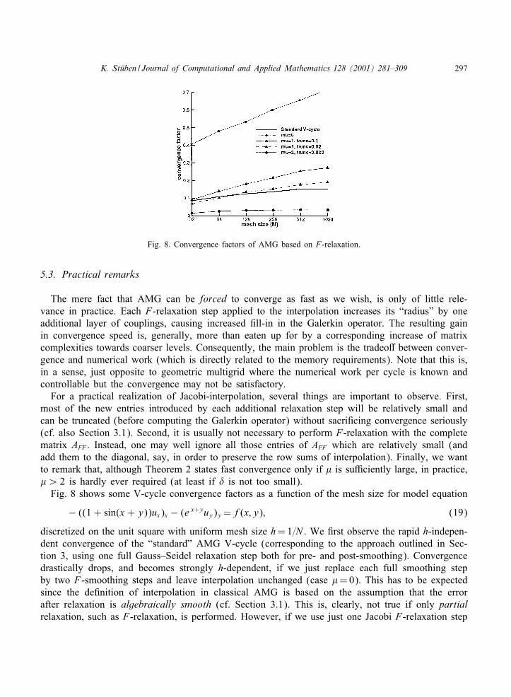
K. St0uben / Journal of Computational and Applied Mathematics 128 (2001) 281–309 297
Fig. 8. Convergence factors of AMG based on F-relaxation.
5.3. Practical remarks
The mere fact that AMG can be forced to converge as fast as we wish, is only of little rele-vance in practice. Each F-relaxation step applied to the interpolation increases its “radius” by oneadditional layer of couplings, causing increased 1ll-in in the Galerkin operator. The resulting gainin convergence speed is, generally, more than eaten up for by a corresponding increase of matrixcomplexities towards coarser levels. Consequently, the main problem is the tradeo3 between conver-gence and numerical work (which is directly related to the memory requirements). Note that this is,in a sense, just opposite to geometric multigrid where the numerical work per cycle is known andcontrollable but the convergence may not be satisfactory.
For a practical realization of Jacobi-interpolation, several things are important to observe. First,most of the new entries introduced by each additional relaxation step will be relatively small andcan be truncated (before computing the Galerkin operator) without sacri1cing convergence seriously(cf. also Section 3.1). Second, it is usually not necessary to perform F-relaxation with the completematrix AFF . Instead, one may well ignore all those entries of AFF which are relatively small (andadd them to the diagonal, say, in order to preserve the row sums of interpolation). Finally, we wantto remark that, although Theorem 2 states fast convergence only if & is su,ciently large, in practice,&¿ 2 is hardly ever required (at least if % is not too small).
Fig. 8 shows some V-cycle convergence factors as a function of the mesh size for model equation
− ((1 + sin(x + y))ux)x − (e x+yuy)y =f(x; y); (19)
discretized on the unit square with uniform mesh size h=1=N . We 1rst observe the rapid h-indepen-dent convergence of the “standard” AMG V-cycle (corresponding to the approach outlined in Sec-tion 3, using one full Gauss–Seidel relaxation step both for pre- and post-smoothing). Convergencedrastically drops, and becomes strongly h-dependent, if we just replace each full smoothing stepby two F-smoothing steps and leave interpolation unchanged (case &=0). This has to be expectedsince the de1nition of interpolation in classical AMG is based on the assumption that the errorafter relaxation is algebraically smooth (cf. Section 3.1). This is, clearly, not true if only partialrelaxation, such as F-relaxation, is performed. However, if we use just one Jacobi F-relaxation step

298 K. St0uben / Journal of Computational and Applied Mathematics 128 (2001) 281–309
to improve interpolation (&=1), convergence becomes comparable to that of the standard cycle.Results are shown using two di3erent truncation parameters, 0.1 and 0.02, respectively. Finally, thecase &=2 (and four partial relaxation steps for smoothing rather than two) gives a convergencewhich is about twice as fast as that of the standard cycle.
We note that, if computational time and memory requirement is taken into account in this example,the standard V-cycle is more e,cient than the others. In particular, the cycle employing &=2is substantially inferior, mainly due to the considerably higher setup cost. This seems typical forapplications for which algebraically smooth errors, in the sense of Section 3.1, can be characterizedsu,ciently well. The heuristic reason is that then, using full smoothing steps, relatively simpleinterpolations of the type outlined in Section 3.1 are usually su,cient to approximate algebraicallysmooth errors and obtain fast convergence. This is no longer true if mere F-smoothing is employedand, generally, additional e3ort needs to be invested to “improve” interpolation by F-relaxation inorder to cope with all those error components which are not a3ected by mere F-smoothing. (Inparticular, note that all error components of the form e are not reduced at all by F-smoothing.)
In general, however, when the characterization of algebraically smooth errors is less straightfor-ward, the use of F-relaxation provides a means to enhance convergence. Further numerical exper-iments employing F-smoothing and Jacobi-interpolation can be found in [28,51]. F-relaxation is aspecial case of a “compatible relaxation” which, in a more general context, is considered in [11].
6. Aggregation-type AMG
In the previous sections, we have considered increasingly complex interpolation approaches. In thissection, we go back and consider the most simple case that each F-variable interpolates from exactlyone C-variable only. We have already pointed out in Section 3.2 that the use of such “one-sided”interpolations is not recommendable. In fact, one important goal of the additional objective introducedin Section 3.2 was just to avoid such extreme interpolations. On the other hand, the resultingmethod is so easy to implement that it, nevertheless, has drawn some attention. We will outlinethe fundamental problems with this approach in Section 6.2 and summarize three possibilities ofimprovement in Sections 6.3–6.5. Since we just want to highlight the main ideas, we restrict ourmotivations to very simple but characteristic (Poisson-like) problems.
6.1. The basic approach
Let us consider C=F-splittings and interpolations (6) where, for each i∈F; wik =1 for just oneparticular k ∈C and zero otherwise. Consequently, the total number of variables can be subdividedinto “aggregates” Ik (k ∈C) where Ik contains (apart from k itself) all indices i corresponding toF-variables which interpolate from variable k (see Fig. 9).
With this notation, the computation of the Galerkin operator becomes very simple. One easilysees that
I Hh AhI h
H =(aHkl ) where aH
kl =∑i∈ Ik
∑j∈ Il
ahij (k; l∈C); (20)
that is, the coe,cient aHkl is just the sum of all cross-couplings between Ik and Il. Obviously,
regarding the coe,cients aHkl , the particular role of the variables k and l (as being C-variables) is

K. St0uben / Journal of Computational and Applied Mathematics 128 (2001) 281–309 299
Fig. 9. Subdivision of 1ne-level variables into aggregates. The arrows indicate which C-variable an F-variable interpolatesfrom.
Fig. 10. Convergence of (a) aggregation-type AMG, (b) classical AMG.
not distinguished from the other variables; the Galerkin operator merely depends on the de�nitionof the aggregates. Consequently, we might as well associate each aggregate Ik with some “new”coarse-level variable which has no direct relation to the C-variable k. The above interpolation thenis nothing else than piecewise constant interpolation from these new coarse-level variables to theassociated aggregates.
Originally, such aggregation-type AMG approaches [52,53,9] have been developed the other wayaround: Coarsening is de1ned by building aggregates (rather than constructing C=F-splittings), a newcoarse-level variable is associated with each aggregate and interpolation I h
H is de1ned to be piecewiseconstant. (That is, the set of coarse-level variables is generally not considered as a subset of the1ne-level ones.) Clearly, for a given subdivision into aggregates to be reasonable, all variables in thesame aggregate should strongly depend on each other. Otherwise, piecewise constant interpolationmakes no real sense.
As expected, an immediate implementation of this simple coarsening and interpolation approachleads to very ine,cient solvers, even if used only as a pre-conditioner. Fig. 10a shows the typicalconvergence of both the V- and the W-cycle, used as stand-alone and as pre-conditioner, in solvingthe model equation (19). Convergence is indeed very slow and exhibits a strong h-dependency. Fora comparison, the much better performance of classical AMG is depicted in Fig. 10b.
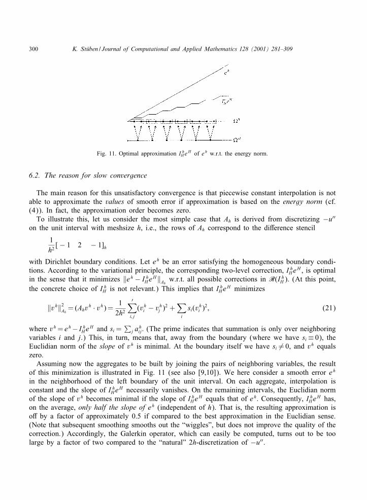
300 K. St0uben / Journal of Computational and Applied Mathematics 128 (2001) 281–309
Fig. 11. Optimal approximation I hH e
H of e h w.r.t. the energy norm.
6.2. The reason for slow convergence
The main reason for this unsatisfactory convergence is that piecewise constant interpolation is notable to approximate the values of smooth error if approximation is based on the energy norm (cf.(4)). In fact, the approximation order becomes zero.
To illustrate this, let us consider the most simple case that Ah is derived from discretizing −u′′on the unit interval with meshsize h, i.e., the rows of Ah correspond to the di3erence stencil
1h2[− 1 2 − 1]h
with Dirichlet boundary conditions. Let eh be an error satisfying the homogeneous boundary condi-tions. According to the variational principle, the corresponding two-level correction, I h
HeH , is optimal
in the sense that it minimizes ‖eh − I hHe
H‖Ahw.r.t. all possible corrections in R(I h
H). (At this point,the concrete choice of I h
H is not relevant.) This implies that I hHe
H minimizes
‖vh‖2Ah=(Ahvh · vh)=
12h2
′∑i; j
(vhi − vh
j )2 +
∑i
si(vhi )
2; (21)
where vh = eh− I hHe
H and si =∑
j ahij. (The prime indicates that summation is only over neighboring
variables i and j.) This, in turn, means that, away from the boundary (where we have si≡ 0), theEuclidian norm of the slope of vh is minimal. At the boundary itself we have si �=0, and vh equalszero.
Assuming now the aggregates to be built by joining the pairs of neighboring variables, the resultof this minimization is illustrated in Fig. 11 (see also [9,10]). We here consider a smooth error eh
in the neighborhood of the left boundary of the unit interval. On each aggregate, interpolation isconstant and the slope of I h
HeH necessarily vanishes. On the remaining intervals, the Euclidian norm
of the slope of vh becomes minimal if the slope of I hHe
H equals that of eh. Consequently, I hHe
H has,on the average, only half the slope of eh (independent of h). That is, the resulting approximation iso3 by a factor of approximately 0.5 if compared to the best approximation in the Euclidian sense.(Note that subsequent smoothing smooths out the “wiggles”, but does not improve the quality of thecorrection.) Accordingly, the Galerkin operator, which can easily be computed, turns out to be toolarge by a factor of two compared to the “natural” 2h-discretization of −u′′.

K. St0uben / Journal of Computational and Applied Mathematics 128 (2001) 281–309 301
If the same strategy is now used recursively to introduce coarser and coarser levels, the abovearguments carry over to each of the intermediate levels and, in particular, each coarser-grid Galerkinoperator is o3 by a factor of 2 compared to the previous one. A simple recursive argument showsthat errors are accumulated from grid to grid and the asymptotic V-cycle convergence factor cannotbe expected to be better than 1− 2−m, where m denotes the number of coarser levels. That is, theV-cycle convergence is strongly h-dependent.
6.3. Improvement by re-scaling the Galerkin operators
The fact that piecewise constant interpolation produces badly scaled AMG components, was thebasis for an improvement introduced in [9]. In that paper, it is demonstrated that convergencecan be substantially improved by just multiplying corrections I h
HeH by some suitable factor �¿ 1
(“over-correction”). This is equivalent to re-scaling the Galerkin operator by 1=�
I Hh AhI h
H→1�I Hh AhI h
H
and leaving everything else unchanged.In case of the simple model equation −u′′ considered in the previous section, �=2 would be the
optimal choice. However, the main arguments carry over to the Poisson equation in 2D and 3D,assuming a uniform grid and the aggregates to be built by 2×2 and 2×2×2 blocks of neighboringvariables, respectively. In case of more general problems and=or di3erent grids, the optimal weight isno longer �=2. Nevertheless, it has been demonstrated in [9] that a slightly reduced value of �=1:8(in order to reduce the risk of “overshooting”) yields substantially improved V-cycle convergencefor various types of problems, if the cycle is used as a pre-conditioner and if the number of coarserlevels is kept 1xed (in [9] four levels are always used). Smoothing is done by symmetric Gauss–Seidel relaxation sweeps.
A comparison of Figs. 10a and 12a shows the convergence improvement if re-scaling by �=1:8is applied to the model equation (19). (In contrast to [9], we here have not restricted the number ofcoarser levels.) Fig. 12a shows that there is indeed a risk of “overshooting”: For larger meshes, theV-cycle starts to diverge. (Note that the above re-scaling destroys the validity of the variational prin-ciple and the iteration process may well diverge.) Using the V-cycle as a pre-conditioner, eliminatesthe problem.
We want to point out that the above comparison shows only the tendency of improvements dueto re-scaling, the concrete gain depends on how the aggregates are chosen precisely (which is notoptimized here and can certainly be improved to some extent). In any case, the gain in convergence,robustness and e,ciency of this (very simple and easily programmable) approach are somewhatlimited, one reason being that a good value of � depends on various aspects such as the concreteproblem, the type of mesh and, in particular, the type and size of the aggregates. For instance, if theaggregates are composed of three neighboring variables (rather than two) in each spatial direction,the same arguments as in the previous section show that the best weight would be � ≈ 3 in case ofPoisson’s equation. If the size of the aggregates strongly varies over the domain, it becomes di,cultto de1ne a good value for �.
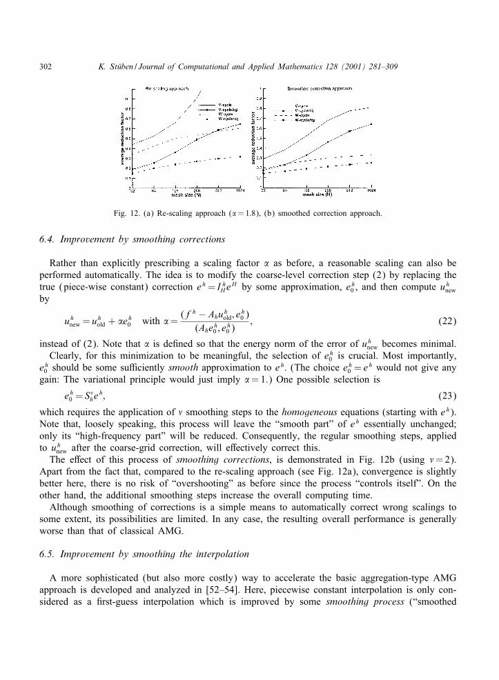
302 K. St0uben / Journal of Computational and Applied Mathematics 128 (2001) 281–309
Fig. 12. (a) Re-scaling approach (�=1:8), (b) smoothed correction approach.
6.4. Improvement by smoothing corrections
Rather than explicitly prescribing a scaling factor � as before, a reasonable scaling can also beperformed automatically. The idea is to modify the coarse-level correction step (2) by replacing thetrue (piece-wise constant) correction eh = I h
HeH by some approximation, eh
0 , and then compute uhnew
by
uhnew = uh
old + �eh0 with �=
(fh − Ahuhold ; e
h0 )
(Aheh0 ; e
h0 )
; (22)
instead of (2). Note that � is de1ned so that the energy norm of the error of uhnew becomes minimal.
Clearly, for this minimization to be meaningful, the selection of eh0 is crucial. Most importantly,
eh0 should be some su,ciently smooth approximation to eh. (The choice eh
0 = eh would not give anygain: The variational principle would just imply �=1.) One possible selection is
eh0 = S�
heh; (23)
which requires the application of � smoothing steps to the homogeneous equations (starting with eh).Note that, loosely speaking, this process will leave the “smooth part” of eh essentially unchanged;only its “high-frequency part” will be reduced. Consequently, the regular smoothing steps, appliedto uh
new after the coarse-grid correction, will e3ectively correct this.The e3ect of this process of smoothing corrections, is demonstrated in Fig. 12b (using �=2).
Apart from the fact that, compared to the re-scaling approach (see Fig. 12a), convergence is slightlybetter here, there is no risk of “overshooting” as before since the process “controls itself”. On theother hand, the additional smoothing steps increase the overall computing time.
Although smoothing of corrections is a simple means to automatically correct wrong scalings tosome extent, its possibilities are limited. In any case, the resulting overall performance is generallyworse than that of classical AMG.
6.5. Improvement by smoothing the interpolation
A more sophisticated (but also more costly) way to accelerate the basic aggregation-type AMGapproach is developed and analyzed in [52–54]. Here, piecewise constant interpolation is only con-sidered as a 1rst-guess interpolation which is improved by some smoothing process (“smoothed
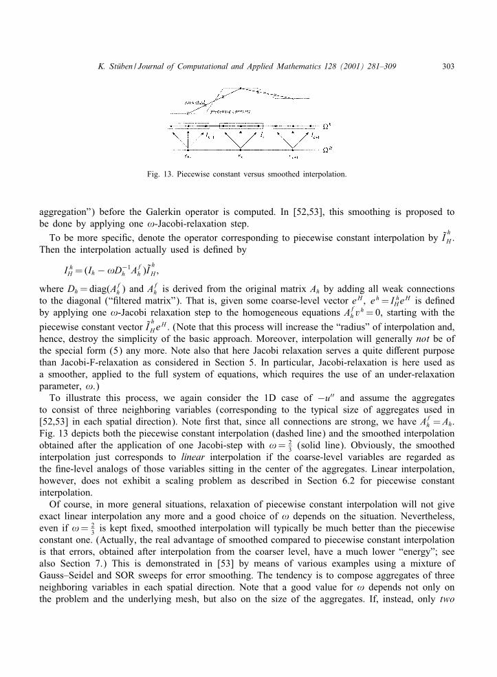
K. St0uben / Journal of Computational and Applied Mathematics 128 (2001) 281–309 303
Fig. 13. Piecewise constant versus smoothed interpolation.
aggregation”) before the Galerkin operator is computed. In [52,53], this smoothing is proposed tobe done by applying one !-Jacobi-relaxation step.
To be more speci1c, denote the operator corresponding to piecewise constant interpolation by IhH .
Then the interpolation actually used is de1ned by
I hH =(Ih − !D−1
h Afh )I
hH ;
where Dh =diag(Afh ) and Af
h is derived from the original matrix Ah by adding all weak connectionsto the diagonal (“1ltered matrix”). That is, given some coarse-level vector eH ; eh = I h
HeH is de1ned
by applying one !-Jacobi relaxation step to the homogeneous equations Afh v
h =0, starting with thepiecewise constant vector I
hH e
H . (Note that this process will increase the “radius” of interpolation and,hence, destroy the simplicity of the basic approach. Moreover, interpolation will generally not be ofthe special form (5) any more. Note also that here Jacobi relaxation serves a quite di3erent purposethan Jacobi-F-relaxation as considered in Section 5. In particular, Jacobi-relaxation is here used asa smoother, applied to the full system of equations, which requires the use of an under-relaxationparameter, !.)To illustrate this process, we again consider the 1D case of −u′′ and assume the aggregates
to consist of three neighboring variables (corresponding to the typical size of aggregates used in[52,53] in each spatial direction). Note 1rst that, since all connections are strong, we have Af
h =Ah.Fig. 13 depicts both the piecewise constant interpolation (dashed line) and the smoothed interpolationobtained after the application of one Jacobi-step with != 2
3 (solid line). Obviously, the smoothedinterpolation just corresponds to linear interpolation if the coarse-level variables are regarded asthe 1ne-level analogs of those variables sitting in the center of the aggregates. Linear interpolation,however, does not exhibit a scaling problem as described in Section 6.2 for piecewise constantinterpolation.
Of course, in more general situations, relaxation of piecewise constant interpolation will not giveexact linear interpolation any more and a good choice of ! depends on the situation. Nevertheless,even if != 2
3 is kept 1xed, smoothed interpolation will typically be much better than the piecewiseconstant one. (Actually, the real advantage of smoothed compared to piecewise constant interpolationis that errors, obtained after interpolation from the coarser level, have a much lower “energy”; seealso Section 7.) This is demonstrated in [53] by means of various examples using a mixture ofGauss–Seidel and SOR sweeps for error smoothing. The tendency is to compose aggregates of threeneighboring variables in each spatial direction. Note that a good value for ! depends not only onthe problem and the underlying mesh, but also on the size of the aggregates. If, instead, only two
304 K. St0uben / Journal of Computational and Applied Mathematics 128 (2001) 281–309
neighbors would be aggregated in each spatial direction, one easily con1rms that ! ≈ 0:5 should bechosen.
In general, classical AMG and AMG based on smoothed aggregation perform comparably if ap-plied to relatively smooth (Poisson-like) problems. A certain advantage of aggregation-type AMGis that it, often, requires less memory than classical AMG (due to its very fast coarsening whichcauses a particularly low operator complexity cA). On the other hand, this is payed for by a re-duced robustness: The aggregation-type code seems to require acceleration by conjugate-gradient tomaintain an acceptable e,ciency and robustness in more complex situations. Since classical AMGputs more e3ort into the construction of interpolation and performs a slower coarsening, its perfor-mance generally depends on aspects such as strong discontinuities only to a lesser extent (for someexamples, see [51]).
7. Further developments and conclusions
Algebraic multigrid provides a general approach to developing robust and e,cient methods forsolving large classes of matrix equations such as those typically arising in the numerical solution ofelliptic PDEs, on structured as well as unstructured grids, in 2D and 3D. The construction of suitableinterpolation operators (including the coarsening process) is crucial for obtaining fast and (nearly)h-independent convergence. Generally, the more e3ort is put into this construction, the faster theconvergence can be, but, unfortunately, the required numerical work may increase even faster. Thatis, the main problem in designing e,cient AMG algorithms is the tradeo3 between convergenceand numerical work, and keeping the balance between the two is the ultimate goal of any practicalalgorithm.
We have summarized and discussed various possibilities to realize concrete AMG algorithms. Formost applications of the type discussed in this paper, methods based on the classical AMG approachstill belong to the most e,cient ones. An extensive list of experiments, based on the originalcode AMG1R5, can be found in [18]. Robustness and e,ciency can substantially be improved, inparticular in case of complex 3D meshes, by employing modi1cations as mentioned in Sections3.1 and 5 (for more details, see [51]). AMG methods based on smoothed aggregation (see Section6.5) are an e,cient alternative to classical AMG, at least if employed as a pre-conditioner ratherthan stand-alone. Further developments and applications which are close to the classical AMG ideasare, for example, contained in [16,23,24,26,32,33,40,62,63]. Related approaches, but with a focus ondi3erent coarsening and interpolation strategies, are, for example, found in [22,27]. Applications ofthe aggregation-type approach in computational Iuid dynamics are found in [30,39,46,60].
However, there are still many applications for which algebraically de1ned interpolation, and hencethe resulting AMG performance, are not yet satisfactory. For instance, one of the major currentresearch activities in AMG aims at its generalization to e,ciently treat systems of PDEs such aslinear elasticity problems. Although AMG has successfully been applied to various cases (see, e.g.,[9,14,31,48,53]), its development has not yet reached a state where a particular approach is wellsettled. However, even for scalar applications, there are still questions about best ways to de1necoarsening and interpolation, for instance, if the given matrix is s.p.d., contains relatively largepositive o3-diagonal entries, and is far from being weakly diagonally dominant. In such cases, theperformance of classical AMG may be only suboptimal.

K. St0uben / Journal of Computational and Applied Mathematics 128 (2001) 281–309 305
It is often possible to avoid such situations by simplifying the given matrix before applying AMG[41]. One can also imagine situations where it would be advantageous (and easy) to provide AMGwith some additional information on the problem at hand. For instance, information on the geometry(in terms of point locations) or more concrete descriptions on what an “algebraically smooth” errorlooks like (e.g. in the form of some user-provided “test-vector(s)”). This additional informationcan be used to 1t AMG’s interpolation in order to approximate certain types of error componentsparticularly well. Straightforward possibilities have already been pointed out in [48].
In the following, we brieIy summarize a few more recent approaches to de1ne interpolation whichaim at increasing the robustness in cases such as those mentioned above.
A new way to construct interpolation (AMGe, [14]) starts from the fact that an algebraicallysmooth error is nothing else but an error which is slow-to-converge w.r.t. the relaxation process.Hence, an algebraically smooth error, generally, corresponds to the eigenvectors of A belongingto the smallest eigen-values. Instead of de1ning interpolation by directly approximating (7), thegoal in [14] is to de1ne interpolation so that the smaller the associated eigenvalue is the betterthe eigenvectors are interpolated. To satisfy this by explicitly computing eigenvectors is, of course,much too expensive. However, in the case of 1nite element methods – assuming the element sti3nessmatrices to be known – one can derive measures (related to measures used in classical multigridtheory) whose minimization allows the determination of local representations of algebraically smootherror components in the above sense. The added robustness has been demonstrated in [14] by meansof certain model applications. However, the approach is still in its infancy. In particular, signi1cantdevelopment work still has to be invested to link the processes of coarsening and interpolationde1nition in order to obtain an optimal algorithm. In any case, it is an interesting new approachwhich has the potential of leading to more generally applicable AMG approaches.
Other algebraic approaches, designed for the solution of equations derived from 1nite-elementdiscretizations, have been considered in [31,58]. Both approaches are aggregation based and thecoarse space basis functions are de1ned so that their energy is minimized in some sense. (In the1nite-element context it is natural to de1ne interpolation implicitly by constructing the coarse spacebasis functions.) This does not require the element sti3ness matrices to be known, but leads toa global (constraint) minimization problem the exact solution of which would be very expensive.However, iterative solution processes are proposed in both papers to obtain approximate solutions,indicating that the extra work (invested in the setup phase) is acceptable. While Wan et al. [58]concentrate on scalar applications, an extension to systems of PDEs (from linear elasticity) is onemajor aspect in [31]. Special attention is paid to the correct treatment of zero-energy modes (e.g.rigid-body modes in case of linear elasticity): such modes should be contained in the span ofthe coarse space basis functions, at least away from Dirichlet boundaries. (Note that, for typicalscalar problems, this corresponds to the requirement that constants should be interpolated exactlyaway from Dirichlet boundaries, cf. (8).) It is interesting that the approach in [31] can be re-garded as an extension of the earlier work [53] on smoothed aggregation: if only one iterationstep is performed to approximately solve the energy minimization problem, the resulting methodcoincides with the smoothed aggregation approach. In contrast to the latter, however, further iter-ations will not increase the support of the basis functions (i.e., the radius of interpolation). Sometest examples in [31] indicate the advantages of this new interpolation in terms of convergencespeed. Unfortunately, however, this bene1t is essentially o3set by the expense of the minimizationsteps.

306 K. St0uben / Journal of Computational and Applied Mathematics 128 (2001) 281–309
There are various other papers with focus on the development of multigrid methods to solve1nite-element problems on unstructured grids. Although some of them are also based on algorithmicalcomponents which are, more or less, algebraically de1ned, most of them are not meant to be algebraicmultigrid solvers in the sense as considered in this paper. We therefore do not want to discuss suchapproaches here further but rather refer, for example, to [15] and the references given therein.
In the approach of [56], A is not assumed to be asymmetric, and interpolation and restrictionare constructed separately. Interpolation, for instance, is constructed so that a smooth error, Sheh, isinterpolated particularly well w.r.t. the Euclidian norm, ‖ ·‖2. More precisely, the attempt is to make
‖Sheh − I hHe
H‖2;where eH denotes the straight injection of Sheh to the coarse level, as small as possible (cf. (4)).In [56], this leads to certain local minimizations which are used to 1nd, for each variable, pairs ofneighboring variables which would allow a good interpolation in the above sense, and, at the sametime, compute the corresponding weights (of both the interpolation and the restriction). Based onthis information, a C=F-splitting is constructed which allows each F-variable to interpolate from oneof the pairs found before. A heuristic algorithm is used to minimize the total number of C-variables.
In this context, we want to point out that, although classical AMG has been developed in thevariational framework, it has successfully been applied to a large number of non-symmetric prob-lems without any modi1cation. This can be explained heuristically but no theoretical justi1cation isavailable at this time. In the context of smoothed aggregation-based AMG, a theoretical analysis canbe found in [25].
An important aspect which has not been addressed in this paper is the parallelization of AMG.An e,cient parallelization of classical AMG is rather complicated and requires certain algorithmicalmodi1cations in order to limit the communication cost without sacri1cing convergence signi1cantly.Most parallelization approaches investigated up to now either refer to simple aggregation-basedvariants (e.g. [46]) or use straightforward domain decomposition techniques (such as Schwarz’ alter-nating method) for parallelization. A parallelization strategy which stays very close to the classicalAMG approach is presented in [29]. Results for complex 3D problems demonstrate that this ap-proach scales reasonably well on distributed memory computers as long as the number of unknownsper processor is not too small. The method discussed in [56] is also available in parallel. Thereare several further ongoing parallelization activities, for instance, at the University of Bonn and theNational Laboratories LLNL [17] and LANL, but no results have been published by now.
It is beyond the scope of this paper to also discuss the variety of hierarchical algebraic approacheswhich are not really related to the multigrid idea in the sense that these approaches are not basedon the fundamental multigrid principles, smoothing and coarse-level correction. There is actually arapid and very interesting ongoing development of such approaches. For completeness, however, weinclude some selected references. Various approaches based on approximate block Gauss elimination(“Schur-complement” methods) are found in [2–5,19,36–38,42,57]. Multi-level structures have alsobeen introduced into ILU-type pre-conditioners, for example, in [49]. Very recently, some hybridmethods have been developed which use ideas from ILU and from multigrid [6–8,43–45]. For afurther discussion, see also [55].
Summarizing, the development of hierarchically operating algebraic methods to e,ciently tacklethe solution of large sparse, unstructured systems of equations, currently belongs to one of the mostactive 1elds of research in numerical analysis. Many di3erent methods have been investigated but,
K. St0uben / Journal of Computational and Applied Mathematics 128 (2001) 281–309 307
by now, none of them is really able to e,ciently deal with all practically relevant problems. Allmethods seem to have their range of applicability but all of them may fail to be e,cient in certainother applications. Hence, the development in this exciting area of research has to be expected tocontinue for the next years.
References
[1] R.E. Alcou3e, A. Brandt, J.E. Dendy, J.W. Painter, The multi-grid method for the di3usion equation with stronglydiscontinuous coe,cients, SIAM J. Sci. Statist. Comput. 2 (1981) 430–454.
[2] O. Axelsson, The method of diagonal compensation of reduced matrix entries and multilevel iteration, J. Comput.Appl. Math. 38 (1991) 31–43.
[3] O. Axelsson, M. Neytcheva, Algebraic multilevel iteration method for Stieltjes matrices, Numer. Linear AlgebraAppl. 1 (3) (1994) 213–236.
[4] O. Axelsson, P.S. Vassilevski, Algebraic multilevel preconditioning methods I, Numer. Math. 56 (1989) 157–177.[5] O. Axelsson, P.S. Vassilevski, Algebraic multilevel preconditioning methods II, SIAM Numer. Anal. 27 (1990)
1569–1590.[6] R.E. Bank, R.K. Smith, The incomplete factorization multigraph algorithm, SIAM J. Sci. Comput., to appear.[7] R.E. Bank, R.K. Smith, The hierarchical basis multigraph algorithm, SIAM J. Sci. Comput., submitted.[8] R.E. Bank, Ch. Wagner, Multilevel ILU decomposition, Numer. Math. 82 (1999) 543–576.[9] D. Braess, Towards algebraic multigrid for elliptic problems of second order, Computing 55 (1995) 379–393.[10] A. Brandt, Algebraic multigrid theory: the symmetric case, Appl. Math. Comput. 19 (1986) 23–56.[11] A. Brandt, General highly accurate algebraic coarsening schemes, Proceedings of the Ninth Copper Mountain
Conference on Multigrid Methods, Copper Mountain, April 11–16, 1999.[12] A. Brandt, S.F. McCormick, J. Ruge, Algebraic multigrid (AMG) for automatic multigrid solution with application
to geodetic computations, Institute for Computational Studies, POB 1852, Fort Collins, Colorado, 1982.[13] A. Brandt, S.F. McCormick, J. Ruge, Algebraic multigrid (AMG) for sparse matrix equations, in: D.J. Evans (Ed.),
Sparsity and its Applications, Cambridge University Press, Cambridge, 1984, pp. 257–284.[14] M. Brezina, A.J. Cleary, R.D. Falgout, V.E. Henson, J.E. Jones, T.A. Manteu3el, S.F. McCormick, J.W. Ruge,
Algebraic multigrid based on element interpolation (AMGe), LLNL Technical Report UCRL-JC-131752, SIAM J.Sci. Comput., to appear.
[15] T. Chan, J. Xu, L. Zikatanov, An agglomeration multigrid method for unstructured grids, Proceedings of the 10thInternational Conference on Domain Decomposition Methods, 1988.
[16] Q. Chang, Y.S. Wong, H. Fu, On the algebraic multigrid method, J. Comput. Phys. 125 (1996) 279–292.[17] A.J. Cleary, R.D. Falgout, V.E. Henson, J.E. Jones, Coarse-grid selection for parallel algebraic multigrid, Proceedings
of the “Fifth International Symposium on Solving Irregularly Structured Problems in Parallel”, Lecture Notes inComputer Science, vol. 1457, Springer, New York, 1998, pp. 104–115.
[18] A.J. Cleary, R.D. Falgout, V.E. Henson, J.E. Jones, T.A. Manteu3el, S.F. McCormick, G.N. Miranda, J.W. Ruge,Robustness and scalability of algebraic multigrid, SIAM J. Sci. Comput., special issue on the “Fifth Copper MountainConference on Iterative Methods”, 1998.
[19] W. Dahmen, L. Elsner, Algebraic Multigrid Methods and the Schur Complement, Notes on Numerical FluidMechanics, 23, Vieweg Verlag, Braunschweig, 1988.
[20] J.E. Dendy Jr., Black box multigrid, J. Comput. Phys. 48 (1982) 366–386.[21] J.E. Dendy, S.F. McCormick, J. Ruge, T. Russell, S. Scha3er, Multigrid methods for three-dimensional petroleum
reservoir simulation, Proceedings of 10th SPE Symposium on Reservoir Simulation, February 6–8, 1989.[22] J. Fuhrmann, A modular algebraic multilevel method, Technical Report Preprint 203, Weierstrass-Institut f&ur
Angewandte Analysis und Stochastik, Berlin, 1995.[23] T. Grauschopf, M. Griebel, H. Regler, Additive multilevel-preconditioners based on bilinear interpolation, matrix
dependent geometric coarsening and algebraic multigrid coarsening for second order elliptic PDEs, Appl. Numer.Math. 23 (1997) 63–96.
308 K. St0uben / Journal of Computational and Applied Mathematics 128 (2001) 281–309
[24] M. Griebel, T. Neunhoe3er, H. Regler, Algebraic multigrid methods for the solution of the Navier–Stokes equationsin complicated geometries, SFB-Bericht Nr. 342=01=96 A, Institut f&ur Informatik, Technische Universit&at M&unchen,1996.
[25] H. Guillard, P. Vanek, An aggregation multigrid solver for convection-di3usion problems on unstructured meshes,Center for Computational Mathematics, University of Denver, Report 130, 1998.
[26] W.Z. Huang, Convergence of algebraic multigrid methods for symmetric positive de1nite matrices with weak diagonaldominance, Appl. Math. Comput. 46 (1991) 145–164.
[27] F. Kickinger, Algebraic multi-grid for discrete elliptic second order problems, Institutsbericht 513, Universit&at Linz,Institut f&ur Mathematik, 1997.
[28] A. Krechel, K. St&uben, Operator dependent interpolation in algebraic multigrid, Proceedings of the Fifth EuropeanMultigrid Conference, Stuttgart, October 1–4, 1996; Lecture Notes in Computational Science and Engineering, vol.3, Springer, Berlin, 1998.
[29] A. Krechel, K. St&uben, Parallel algebraic multigrid based on subdomain blocking, Parallel Comput., to appear.[30] R.D. Lonsdale, An algebraic multigrid solver for the Navier–Stokes equations on unstructured meshes, Int. J. Numer.
Methods Heat Fluid Flow 3 (1993) 3–14.[31] J. Mandel, M. Brezina, P. Vanek, Energy optimization of algebraic multigrid bases, UCD=CCM Report 125, 1998.[32] S. McCormick, J. Ruge, Algebraic multigrid methods applied to problems in computational structural mechanics, in:
State-of-the-Art Surveys on Computational Mechanics, ASME, New York, 1989, pp. 237–270.[33] R. Mertens, H. De Gersem, R. Belmans, K. Hameyer, D. Lahaye, S. Vandewalle, D. Roose, An algebraic multigrid
method for solving very large electromagnetic systems, IEEE Trans. Magn. 34 (1998), to appear.[34] W.A. Mulder, A new multigrid approach to convection problems, J. Comput. Phys. 83 (1989) 303–323.[35] N.H. Naik, J. van Rosendale, The improved robustness of multigrid elliptic solvers based on multiple semicoarsened
grids, SIAM Numer. Anal. 30 (1993) 215–229.[36] Y. Notay, An e,cient algebraic multilevel preconditioner robust with respect to anisotropies, in: O. Axelsson, B.
Polman (Eds.), Algebraic Multilevel Iteration Methods with Applications, Department of Mathematics, University ofNijmegen, 1996, pp. 111–228.
[37] Y. Notay, Using approximate inverses in algebraic multilevel methods, Numer. Math. 80 (1998) 397–417.[38] Y. Notay, Optimal V-cycle algebraic multilevel preconditioning, Numer. Linear Algebra Appl., to appear.[39] M. Raw, A coupled algebraic multigrid method for the 3D Navier–Stokes equations, Report: Advanced Scienti1c
Computing Ltd., 554 Parkside Drive, Waterloo, Ontario N2L 5Z4, Canada.[40] H. Regler, Anwendungen von AMG auf das Plazierungsproblem beim Layoutentwurf und auf die numerische
Simulation von Str&omungen, Ph.D. thesis, TU M&unchen, 1997.[41] S. Reitzinger, Algebraic multigrid and element preconditioning I, SFB-Report 98-15, University Linz, Austria,
December 1998.[42] A.A. Reusken, Multigrid with matrix-dependent transfer operators for a singular perturbation problem, Computing
50 (3) (1993) 199–211.[43] A.A. Reusken, A multigrid method based on incomplete Gaussian elimination, Eindhoven University of Technology,
Report RANA 95-13, ISSN 0926-4507, 1995.[44] A.A. Reusken, On the approximate cyclic reduction preconditioner, Report 144, Institut f&ur Geometrie und Praktische
Mathematik, RWTH Aachen, 1997. SIAM J. Sci. Comput., to appear.[45] A.A. Reusken, Approximate cyclic reduction preconditioning, in: W. Hackbusch, G. Wittum (Eds.), Multigrid
Methods, Vol. 5, Lecture Notes in Computational Science and Engineering, Vol. 3, Springer, Berlin, 1998, pp.243–259.
[46] G. Robinson, Parallel computational Iuid dynamics on unstructured meshes using algebraic multigrid, in: R.B. Pelz,A. Ecer, J. H&auser (Eds.), Parallel Computational Fluid Dynamics, Vol. 92, Elsevier, Amsterdam, 1993.
[47] J.W. Ruge, K. St&uben, E,cient solution of 1nite di3erence and 1nite element equations by algebraic multigrid(AMG), in: D.J. Paddon, H. Holstein (Eds.), Multigrid Methods for Integral and Di3erential Equations, The Instituteof Mathematics and its Applications Conference Series, New Series vol. 3, Clarendon Press, Oxford, 1985, pp.169–212.
[48] J.W. Ruge, K. St&uben, Algebraic multigrid (AMG), in: S.F. McCormick (Ed.), Multigrid Methods, Frontiers inApplied Mathematics, Vol. 5, SIAM, Philadelphia, 1986.
K. St0uben / Journal of Computational and Applied Mathematics 128 (2001) 281–309 309
[49] Y. Saad, ILUM: a multi-elimination ILU preconditioner for general sparse matrices, SIAM J. Sci. Comput. 17 (1996)830–847.
[50] K. St&uben, Algebraic multigrid (AMG): Experiences and comparisons, Appl. Math. Comput. 13 (1983) 419–452.[51] K. St&uben, Algebraic multigrid (AMG): an introduction with applications, in: U. Trottenberg, C.W. Oosterlee, A.
Sch&uller (Eds.), Multigrid, Academic Press, New York, 2000. Also GMD Report 53, March 1999.[52] P. Vanek, J. Mandel, M. Brezina, Algebraic multigrid on unstructured meshes, University of Colorado at Denver,
UCD=CCM Report No. 34, 1994.[53] P. Vanek, J. Mandel, M. Brezina, Algebraic multigrid by smoothed aggregation for second and fourth order elliptic
problems, Computing 56 (1996) 179–196.[54] P. Vanek, M. Brezina, J. Mandel, Convergence of algebraic multigrid based on smoothed aggregation, UCD=CCM
Report 126, 1998. Numer. Math., submitted.[55] C. Wagner, Introduction to algebraic multigrid, Course notes of an algebraic multigrid course at the University of
Heidelberg in the Wintersemester 1998=99, http:==www.iwr.uni-heidelberg.de= ∼ Christian.Wagner, 1999.[56] C. Wagner, On the algebraic construction of multilevel transfer operators, IWR-Report, Universit&at Heidelberg,
Computing (2000).[57] C. Wagner, W. Kinzelbach, G. Wittum, Schur-complement multigrid – a robust method for groundwater Iow and
transport problems, Numer. Math. 75 (1997) 523–545.[58] W.L. Wan, T.F. Chan, B. Smith, An energy minimization interpolation for robust multigrid methods, Department of
Mathematics, UCLA, UCLA CAM Report 98-6, 1998.[59] T. Washio, C.W. Oosterlee, Flexible multiple semicoarsening for 3D singularly perturbed problems, SIAM J. Sci.
Comput. 19 (1998) 1646–1666.[60] R. Webster, An algebraic multigrid solver for Navier–Stokes problems in the discrete second order approximation,
Int. J. Numer. Methods Fluids 22 (1996) 1103–1123.[61] P. Wesseling, C.W. Oosterlee, Geometric multigrid with applications to computational Iuid dynamics, this volume,
Comput. Appl. Math. 128 (2001) 311–334.[62] L. Zaslavsky, An adaptive algebraic multigrid for multigroup neutron di3usion reactor core calculations, Appl. Math.
Comput. 53 (1993) 13–26.[63] L. Zaslavsky, An adaptive algebraic multigrid for reactor critically calculations, SIAM J. Sci. Comput. 16 (1995)
840–847.
Journal of Computational and Applied Mathematics 128 (2001) 311–334www.elsevier.nl/locate/cam
Geometric multigrid with applications to computational $uiddynamics
P. Wesselinga ; ∗, C.W. OosterleebaJ.M. Burgers Center and Delft University of Technology, Faculty of Technical Mathematics and Informatics,
Mekelweg 4, 2628 CD Delft, The NetherlandsbUniversity of Cologne and GMD, Institute for Algorithms and Scienti(c Computing, D-53754 Sankt Augustin,
Germany
Received 5 July 1999; received in revised form 29 November 1999
Abstract
An overview is given of the development of the geometric multigrid method, with emphasis on applications in computa-tional $uid dynamics over the last ten years. Both compressible and incompressible $ow problems and their correspondingmultigrid solution methods are discussed. The state of the art is described with respect to methods employed in industryas well as the multigrid e3ciency obtained in academic applications. c© 2001 Elsevier Science B.V. All rights reserved.
MSC: 65N55; 76Mxx
Keywords: Multigrid; Nonlinear problems; Computational $uid dynamics
1. Introduction
The multigrid or multilevel approach has the unique potential of solving many kinds of mathe-matical problems with N unknowns with O(N ) work. As discussed in [15], this applies to diverseareas such as integral equations, or optimization methods in various scienti?c disciplines. Complexityof O(N ) has been shown theoretically for discretizations of a large class of elliptic linear partialdi@erential equations [38,4,43–45,149].
We can distinguish between algebraic multigrid (AMG) [121] and geometric multigrid. In algebraicmultigrid no information is used concerning the grid on which the governing partial di@erentialequations are discretized. Therefore, it might be better to speak of algebraic multilevel methods. Ingeometric multigrid, coarse grids are constructed from the given ?ne grid, and coarse grid corrections
∗ Corresponding author.E-mail address: [email protected] (P. Wesseling).
0377-0427/01/$ - see front matter c© 2001 Elsevier Science B.V. All rights reserved.PII: S 0377-0427(00)00517-3

312 P. Wesseling, C.W. Oosterlee / Journal of Computational and Applied Mathematics 128 (2001) 311–334
are computed using discrete systems constructed on the coarse grids. Constructing coarse grids from?ne grids by agglomeration of ?ne grid cells is easy when the ?ne grid is structured, but not if the?ne grid is unstructured. That is where algebraic multigrid becomes useful. Unfortunately, AMG isless developed than geometric multigrid for the applications considered here. Algebraic multigrid iscovered by K. StGuben in another paper in this issue. The present paper is about geometric multigrid.
For remarks on early multigrid history, see [150,152]. In the early seventies, there were methodsalready available with low computational complexity, such as solution methods based on fast Fouriertransforms, resulting in O(N logN ) work. But these methods are restricted to special classes ofproblems, such as separable partial di@erential equations on cubic domains. Multigrid, however, ismuch more robust: it is e3cient for a much wider class of problems. The interest of practitionersof large-scale scienti?c computing in multigrid was particularly stimulated by the 1977 paper [11]of Achi Brandt, generally regarded as a landmark in the ?eld. Two series of conferences dedicatedto multigrid were set up: the European Multigrid Conferences (EMG): Cologne (1981; 1985), Bonn(1991), Amsterdam (1993), Stuttgart (1996), Ghent (1999), and in the US the Copper MountainConferences on multigrid, held bi-annually from 1983 until the present. Proceedings of the Europeanmeetings have appeared in [46,48,49,54,50] and of the Copper Mountain Conferences in specialissues of journals: Applied Numerical Mathematics (Vol. 13, 1983; Vol. 19, 1986), Communicationsin Applied Numerical Methods (Vol. 8, 1992), SIAM Journal of Numerical Analysis (Vol. 30, 1993),Electronic Transactions on Numerical Analysis (Vol. 6, 1996). Another rich source of informationon multigrid is the MGNet website maintained by C.C. Douglas: http:==www.mgnet.org.
Introductions to multigrid methods can be found in [11,17,47,134,152], to be collectively referredto in the sequel as the basic literature. A thorough introduction to multigrid methods is given in[47]. The introduction in [152] requires less mathematical background and is more oriented towardsapplications. In Chapter 9 of [152] the basic principles and the state of the art around 1990 ofmultigrid for computational $uid dynamics is described. Therefore here we will not dwell much onthe basic principles, and con?ne ourselves mainly to developments that have taken place during thelast decade.
Computational Fluid Dynamics (CFD) gives rise to very large systems requiring e3cient solutionmethods. Not surprisingly, multigrid found applications in CFD at an early stage. The compressiblepotential equation was solved with multigrid in 1976 [131], the incompressible Navier–Stokes equa-tions shortly after [12,148]. Over the years, multigrid has become closely intertwined with CFD,and has become an ingredient in major CFD codes. The viscous $ow around a complete aircraftcon?guration can now be computed thanks to the availability of multigrid solvers [60], and alsocomplex industrial $ows in machinery are computed successfully with multigrid.
However, as remarked in [15], full textbook multigrid e3ciency has not yet been achieved inrealistic engineering applications in CFD in general. An important reason for this is that in CFDwe often have to deal with singular perturbation problems. This gives rise to grids with cells withhigh aspect ratios. Another reason is that the governing equations may show elliptic or parabolicbehavior in one part of the domain and hyperbolic behavior in another part of the domain. Thisrequires careful design of both the discretization and the solver, putting a premium on robustness.With the increasing complexity of CFD applications (most of all due to the grid structures onwhich the equations are discretized), the demand for robustness of solution methods is increasingeven more. Industrial practice is heading towards unstructured grids, more complex $ow modeling,time-dependent problems and multidisciplinary applications. These developments pose new challenges

P. Wesseling, C.W. Oosterlee / Journal of Computational and Applied Mathematics 128 (2001) 311–334 313
for multigrid research. The potential for large further gains is there, and consequently multigridremains an active research topic in CFD. Ways for improvement are pointed out in [15,16]. Thecurrent state of the art is surveyed below.
The ?eld of computational $uid dynamics is too diverse and multigrid can be implemented intoo many ways to make a self-contained synopsis possible within the con?nes of a journal article.Therefore our descriptions will be eclectic, global and fragmentary, but we will cast our net widein referring to the literature after 1990 for further details.
2. Multigrid basics
First, we present a brief description of multigrid principles. For further information one may consultthe basic literature. To establish notation and terminology, we start by formulating the basic two-gridalgorithm. Let us have a system of m partial di@erential equations on a domain �, discretized on agrid G⊂�. The resulting nonlinear algebraic system is denoted as
N (u) = b; u ∈ U = {u : G → Rm}; (1)
where U is the space of grid functions on G. For the moment, the problem is assumed to beindependent of time. Let there also be a coarse grid NG⊂� with fewer nodes than G. Overbarsdenote coarse grid quantities.
2.1. The nonlinear multigrid method
The basic two-grid algorithm is given by
Choose u0
Repeat until convergence:begin
(1) S1(u0; u1=3; b); r = b− N (u1=3);(2) Choose Nu�; s; Nb= NN ( Nu�) + �Rr;(3) NS( Nu�; Nu
2=3; Nb);(4) u2=3 = u1=3 + 1
�P( Nu2=3 − Nu�);
(5) S2(u2=3; u1; b);(6) u0 = u1;
end
Step (1) (pre-smoothing) consists of a few iterations with some iterative method for the ?ne gridproblem (1) with initial iterate u0 and result u1=3. In step (2), Nu� is an approximation on the coarsegrid of the exact solution, used to remain on the correct solution branch and/or to linearize thecoarse grid correction problem. One may take, for example, Nu�= Ru1=3, with R : U → NU a restrictionoperator from the ?ne to the coarse grid. But it may be more economical to keep Nu� ?xed duringtwo-grid iterations, if NN ( Nu�) is expensive, or if Nu� is used to construct an expensive Jacobian. In step(2), � is a parameter which, if chosen small enough, ensures solvability of the coarse grid problem,
314 P. Wesseling, C.W. Oosterlee / Journal of Computational and Applied Mathematics 128 (2001) 311–334
given by
NN (u) = Nb ≡ NN (u�) + �Rr; (2)
where NN is a coarse grid approximation to N , obtained, for example, by discretization of the under-lying system of partial di@erential equations on NG. Furthermore, R : U → NU is a ?ne to coarse gridrestriction operator, that need not be the same as R. In step (3), NS stands for solving the coarse gridproblem (2) approximately by some iteration method with initial guess Nu� and result Nu 2=3. In step(4), the coarse grid correction is added to the current ?ne grid iterate. Here, P is a prolongation orinterpolation operator P : NU → U . In step (5) post-smoothing takes place.
With � = 1, we obtain the well-known Full Approximation Scheme (FAS) [11], which is mostcommonly used in CFD. The nonlinearity of the problems enters in the smoothing operators S1; S2and NS. Global linearization is not necessary, so that there is no need to store a global Jacobian, whichis, moreover, frequently very ill-conditioned in CFD. For many problems, however, the nonlinearitycan also be handled globally, resulting in a sequence of linear problems that can be solved e3cientlywith linear multigrid. The multigrid method is obtained if solution of the coarse grid problem instep (3) is replaced by � iterations with the two-grid method, employing a still coarser grid, andso on, until the coarsest grid is reached, where one solves more or less exactly. With � = 1 or� = 2, the V- or W-cycle is obtained, respectively. If N is the number of unknowns on G andN=� is the number of nodes on NG, then the above multigrid algorithm requires O(N ) storage and,for accuracy commensurable with discretization accuracy, O(N logN ) work, if �¡�. To get O(N )work, the multigrid cycles must be preceded by nested iteration, also called full multigrid; see thebasic literature. Starting on a coarse grid and re?ning this grid successively leads to a well-de?nedgrid hierarchy also on unstructured grids (see, for example [7]). For a given unstructured grid itis usually not di3cult to de?ne a sequence of ?ner grids and a corresponding multigrid method.However, it might be di3cult to de?ne a sequence of coarser grids starting from an irregular ?negrid [21]. This is where AMG [121] comes into play.
A natural generalization of multigrid is to combine it with locally re?ned grids. This leads to theMultilevel Adaptive Technique (MLAT) [11,5] or to the Fast Adaptive Composite Method (FAC)[90]. The locally re?ned regions are incorporated as extra additional levels in multigrid where allmultigrid components like smoothing are de?ned with minor modi?cations, see [11,90] for details.
The favorable O(N ) convergence behavior depends on satisfying the smoothing property andthe approximation property [47]. The smoothing property requires that the smoothing processesS1 and S2 make the error between discrete solution and current approximation smooth. In not toodi3cult cases this can be checked by frozen coe3cients Fourier analysis [11,134,152], leading tothe determination of the smoothing factor. The approximation property says something about theaccuracy of the coarse grid correction applied in step (4). Extrapolating from what is known fromsimple cases, this implies roughly, for example, that P and R, when applied to a given variable andits corresponding residual, should satisfy
mP + mR ¿M: (3)
Here, orders mP; mR of P and R are de?ned as the highest degree plus one of polynomials that areinterpolated exactly by P or �RT, respectively, with � a scaling factor, RT the transpose of R, andM the order of the highest derivative of the unknown concerned that occurs in the partial di@erentialequation. For instance, for the Euler equations, we have M = 1, whereas for the Navier–Stokes
P. Wesseling, C.W. Oosterlee / Journal of Computational and Applied Mathematics 128 (2001) 311–334 315
equations we have M = 1 for the pressure but M = 2 for velocity components. No requirements areknown for R.
2.2. The smoothing method
An important issue is the robustness of the smoother. This implies that the smoother should bee3cient for a su3ciently large class of problems. Two model problems that represent circumstancesencountered in CFD practice are the convection-di@usion equation and the rotated anisotropic di@u-sion equation, given by, respectively
cux + suy − �(uxx + uyy) = 0; (4)
− (�c2 + s2)uxx − 2(�− 1)csuxy − (�s2 + c2)uyy = 0; (5)
where c = cos�; s = sin�, and � and � are parameters. The ?rst equation contains the e@ect ofstrong convection (if ��1) and is related to hyperbolic systems; a method that does not work fora scalar hyperbolic equation (� = 0) is likely to fail for a system. The second equation models thee@ect of large mesh aspect ratios, equivalent to ��1 on an isotropic grid, and grid nonorthogonality(� = 0), giving rise to mixed derivatives in boundary-?tted coordinates. A smoothing method maybe called robust if it works for all � and �. For a multigrid method that is robust for the testproblems (4) and (5) one may have some hope of success in application to the governing equationsof CFD. Fourier smoothing analysis for the simple test problems above is easy, and smoothingfactors for many methods are reported in [151,152,104,169], and for some three-dimensional casesin [67,136]. For the two-dimensional case, robust smoothing methods exist. They are basically ofline-Gauss–Seidel type and ILU type; a list is given in Section 7:12 of [152]. For the simple testproblems (4) and (5), it can be said that e3cient and robust multigrid smoothers and correspondingmultigrid methods are available, even of black-box type for problems on structured grids, see [162].What has kept CFD applications away from textbook multigrid e3ciency is the generalization fromthe scalar case to the case of systems of partial di@erential equations, the di3culty of making thecoarse grid correction su3ciently accurate, and ?nding e3cient smoothers for higher-order upwinddiscretizations with limiters. Furthermore, application of multigrid to unstructured grids has startedonly recently, and further development is necessary for achieving textbook multigrid e3ciency inthis context.
The historical development of multigrid in CFD has been such that smoothing methods come intwo $avors: basic iterative methods (BIMs) and multistage (MS) (Runge–Kutta) methods. Assuminginstead of (1) a linear problem Au= b, a BIM is given by
Mun+1 = Nun + b; A=M − N: (6)
Typical examples of BIMs are methods of Gauss–Seidel type and of incomplete LU factorization(ILU) type. MS smoothers for the nonlinear system (1) are obtained by arti?cially creating a systemof ordinary di@erential equations:
dudt
= N (u)− b: (7)

316 P. Wesseling, C.W. Oosterlee / Journal of Computational and Applied Mathematics 128 (2001) 311–334
MS methods of the following type are used:
u(0) = un;
u(k) = u(0) − ck N (u(k−1)) + ck b; k = 1; : : : ; p; (8)
un+1 = u(p);
where is a time step. The appearance of time in our algebraic problem comes as a surprise, butin fact this application of MS to solve an algebraic system is old wine in a new bag. In the linearcase, where N (u) = Au, we obtain by elimination of u(k):
un+1 = Pp(− A)un + Qp−1(− A)b; (9)
with the ampli?cation polynomial Pp of degree p given by
Pp(z) = 1 + z(cp + cp−1z(1 + cp−2z(: : : (1 + c1z) : : :); (10)
and Qp−1 a polynomial that we will not write down. It follows that MS is an iterative method ofthe type
un+1 = Sun + Tb; S = Pp(− A): (11)
Methods for which the iteration matrix S is a polynomial of the matrix of the system to be solvedare well-known in numerical linear algebra, and are called semi-iterative methods; see [142] for thetheory of such methods. In the multigrid context, the MS coe3cients ck are not chosen to optimizetime accuracy or stability, but the smoothing performance. Because for stationary problems time isan artifact, need not be the same for all grid cells, but can vary, such that ck is optimal forsmoothing. Grids with large aspect ratios are generic for Navier–Stokes applications, due to theneed to resolve thin boundary layers. Smoothing analysis reveals that when high mesh aspect ratiosoccur, modeled by test problem (5) by choosing � = 0; ��1, then point-wise smoothers such asGauss–Seidel and MS, are not satisfactory. The unknowns in certain subsets of the grid points shouldbe updated together, leading to line-Gauss–Seidel or ILU [162,163].
In the MS case, implicit stages could be included, but this avenue has not been followed system-atically. Instead, implicit residual averaging is applied. After a MS stage, the residual
r(k) = b− Au(k)
is replaced by r(k) satisfying
Br(k) = r(k); (12)
with B such that B−1 has a smoothing e@ect, and such that (12) is cheap to solve. For details, see[83]; tuning parameters are involved.
These ways to obtain a robust smoother clearly have drawbacks. Extensions to systems of dif-ferential equations leads to the need to solve subsystems that are more involved and costly thantri-diagonal systems encountered in implicit residual averaging or line-Gauss–Seidel for the scalarcase. Parallelizability is likely to be impaired. An alternative is to strengthen the coarse grid correc-tion instead of the smoother. This can be done by constructing the coarse grid by semi-coarsening,i.e., the mesh-size is doubled only in selected directions, such that the coarse grid becomes more

P. Wesseling, C.W. Oosterlee / Journal of Computational and Applied Mathematics 128 (2001) 311–334 317
isotropic than its parent ?ne grid. This approach, although not novel, has only recently started tohave an impact of practical CFD; we will return to semi-coarsening below.
In three dimensions, the situation is less satisfactory, see [67]. Typical reference model problemsin 3D can be
scux + cuy + ssuz − �(uxx + uyy + uzz) = 0; (13)
where c = cos�; s= sin�; s= sin &; c = cos & and �; & and � are parameters, and
− �1uxx − �2uyy − �3uzz = 0: (14)
If a strong coupling of unknowns in two space directions in (14) exists, it is not possible to usecheap basic (collective) point or line Gauss–Seidel type smoothers and still obtain a fast and e3cientmultigrid method. The strong coupling of unknowns should be taken into account. This means thatplane smoothers, that update all unknowns in a plane simultaneously, have to be applied. However,the coupled system in a plane, even for scalar equations, does not result in a tri-diagonal system aswith line smoothers, but in a more general sparse system. It is found that often, an inexact (iterative)solution method, like one multigrid V-cycle in a 2D plane, is su3cient for an overall e3cient 3Dsolution method [136,103]. In this way a relatively cheap plane solver can be obtained for certainproblems.
It helps considerably in ?nding e3cient smoothers if the Jacobian of N (u) is close to an M -matrix,as explained in Section 4.2 of [152]. Unfortunately, Godunov’s order barrier theorem [42] impliesthat this can be the case only for ?rst-order accurate schemes (in the linear case), so that weare restricted to ?rst-order upwind schemes. This is unsatisfactory. Generally speaking, engineeringpractice requires second-order accuracy. One way around this is to use defect correction. Suppose,we have a ?rst-order discretization N1(u) for which we have a good smoother, and a second-orderscheme N2(u) that we would prefer to use. Defect correction works as follows:
begin Solve N1(y) = b;for i = 1(1) n do
Solve N1(y) = b− N2(y) + N1(y);y = y;
odend
It su3ces to take n=1 or 2 to achieve second-order accuracy. But there are smoothers that workfor second-order schemes, so that defect correction is not necessary; see [34,1,104].
2.3. The coarse grid correction
In this section, we discuss several issues related to the coarse grid correction that are relevant forCFD problems. In linear multigrid, there are two ways to approximate the ?ne grid operator on coarsegrids, namely coarse grid discretization approximation and coarse grid Galerkin approximation. Withthe discretization approximation the coarse grid operator is obtained by rediscretizing the governingdi@erential equations on the coarse grids. With the Galerkin approximation one puts
NA= RAP:
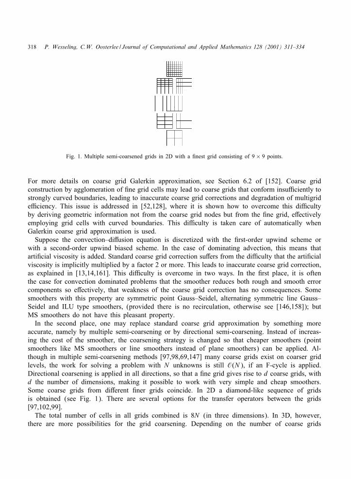
318 P. Wesseling, C.W. Oosterlee / Journal of Computational and Applied Mathematics 128 (2001) 311–334
Fig. 1. Multiple semi-coarsened grids in 2D with a ?nest grid consisting of 9× 9 points.
For more details on coarse grid Galerkin approximation, see Section 6:2 of [152]. Coarse gridconstruction by agglomeration of ?ne grid cells may lead to coarse grids that conform insu3ciently tostrongly curved boundaries, leading to inaccurate coarse grid corrections and degradation of multigride3ciency. This issue is addressed in [52,128], where it is shown how to overcome this di3cultyby deriving geometric information not from the coarse grid nodes but from the ?ne grid, e@ectivelyemploying grid cells with curved boundaries. This di3culty is taken care of automatically whenGalerkin coarse grid approximation is used.
Suppose the convection–di@usion equation is discretized with the ?rst-order upwind scheme orwith a second-order upwind biased scheme. In the case of dominating advection, this means thatarti?cial viscosity is added. Standard coarse grid correction su@ers from the di3culty that the arti?cialviscosity is implicitly multiplied by a factor 2 or more. This leads to inaccurate coarse grid correction,as explained in [13,14,161]. This di3culty is overcome in two ways. In the ?rst place, it is oftenthe case for convection dominated problems that the smoother reduces both rough and smooth errorcomponents so e@ectively, that weakness of the coarse grid correction has no consequences. Somesmoothers with this property are symmetric point Gauss–Seidel, alternating symmetric line Gauss–Seidel and ILU type smoothers, (provided there is no recirculation, otherwise see [146,158]); butMS smoothers do not have this pleasant property.
In the second place, one may replace standard coarse grid approximation by something moreaccurate, namely by multiple semi-coarsening or by directional semi-coarsening. Instead of increas-ing the cost of the smoother, the coarsening strategy is changed so that cheaper smoothers (pointsmoothers like MS smoothers or line smoothers instead of plane smoothers) can be applied. Al-though in multiple semi-coarsening methods [97,98,69,147] many coarse grids exist on coarser gridlevels, the work for solving a problem with N unknowns is still O(N ), if an F-cycle is applied.Directional coarsening is applied in all directions, so that a ?ne grid gives rise to d coarse grids, withd the number of dimensions, making it possible to work with very simple and cheap smoothers.Some coarse grids from di@erent ?ner grids coincide. In 2D a diamond-like sequence of gridsis obtained (see Fig. 1). There are several options for the transfer operators between the grids[97,102,99].
The total number of cells in all grids combined is 8N (in three dimensions). In 3D, however,there are more possibilities for the grid coarsening. Depending on the number of coarse grids
P. Wesseling, C.W. Oosterlee / Journal of Computational and Applied Mathematics 128 (2001) 311–334 319
chosen, a point or a line smoother must be used to obtain a robust 3D multiple semi-coarsening-basedsolution method. A multiple semi-coarsening variant that uses a coarsening strategy such that linesmoothers guarantee robustness for 3D reference problems is presented in [147]. A reduction ofthe computational overhead can be achieved by <exible multiple semi-coarsening: only if strongcouplings in certain directions exist [147], the semi-coarsening process is continued in that direc-tion.
The second variant is directional coarsening: ?ne grid cells are coarsened in one direction only,by removing only the largest cell faces, so that coarsening is done only in a direction roughlyperpendicular to re?nement zones. When the coarse grid has become su3ciently isotropic, one canswitch to full coarsening. This approach is commonly used for compressible Navier–Stokes equations,to be discussed in Section 4.2. Directional semi-coarsening combined with line relaxation is presentedin [27].
2.4. Structured and unstructured grids
Grid generation is one of the most time consuming activities of the CFD practitioner. It is usuallythe main bottleneck for project turn-around time. In comparison, solver CPU time plays a minorrole. This achievement is for a large part due to multigrid. In the past, much e@ort has gone intodevelopment of tools for the generation of structured grids. In such grids, the number of cells thatshare a common vertex is uniform in the interior of the domain. The approach is to divide thedomain in subdomains, each of which is mapped by a boundary-?tted coordinate mapping to acube, in which a uniform grid is generated, the image of which gives a boundary-?tted curvilineargrid in the subdomain. In order to cope with the geometric complexity of engineering applications,the subdomain decomposition must be unstructured, leading to multiblock block-structured grids.On structured grids algorithms can be formulated that run fast on vector computers, less computermemory is required, and coarse grid generation for multigrid and the implementation of transfer op-erators between grids is straightforward. These are the main advantages of structured grids. Despiteintensive research e@orts, however, it has turned out to be not possible to automate the genera-tion of structured grids to a su3cient extent to reduce the amount of human labor involved to alow level. In particular, the generation of the domain decomposition requires much time from theuser.
As a consequence, unstructured grids are now getting more and more attention. Not only arethese grids easier to generate than structured grids, they also lend themselves better to adaptivediscretization, since it is relatively easy to insert and remove grid points. The development of accuratediscretizations and e3cient solution methods is more di3cult than for structured grids. This is nowan active ?eld of research, and much remains to be done. We will give some pointers to recentwork, but it is too early for a review. We will concentrate mainly on structured grids, which arestill mostly used today.
A third type of grid consists of the union of locally overlapping grids that together cover thedomain. The local grids are usually structured. The $exibility o@ered by this kind of grid is especiallyuseful for $ows in which boundary parts move relatively to each other. Furthermore, this is a wayto include adaptivity in the structured grid context. The multigrid principles are the same as forstructured grids. We will not discuss overlapping grids. Examples may be found in [3,55,22,138].

320 P. Wesseling, C.W. Oosterlee / Journal of Computational and Applied Mathematics 128 (2001) 311–334
3. Incompressible �ow
Uni?ed methods that treat compressible and incompressible $ows in a uniform way are emerging(see [9] and references quoted there). Uni?ed methods departing from incompressible Navier–Stokesadopt corresponding solution methods, whereas low Mach equations arising from preconditioningcompressible formulations are solved by compressible solution methods. Standard computing meth-ods for compressible and incompressible $ow di@er substantially, and will therefore be discussedseparately. We start with the incompressible case.
We will assume that discretization takes place on boundary-?tted structured grids. The $ow isgoverned by the incompressible Navier–Stokes equations. For the high Reynolds numbers occurringin most applications thin boundary layers occur, necessitating locally re?ned grids, giving rise tohigh mesh aspect ratios (104 or even more). The primitive variables are commonly used. The so-lution of d momentum equations (d is the number of dimensions) and the continuity equation isrequired. The discretized continuity equation serves as an algebraic constraint, see any textbook onthe incompressible Navier–Stokes equations, so that after discretization in space the incompressibleNavier–Stokes equations constitute a di@erential-algebraic system (of index two), and the pressureacts as a Lagrangean multiplier, mathematically speaking.
Often, a semi-heuristic turbulence model is used to predict time-averaged $ow variables basedon a compromise between accuracy, memory requirements and computing time. More completemodels such as large-eddy simulation and direct numerical simulation are time dependent and canbe e3ciently implemented with explicit time-stepping schemes. In these models an algebraic pressurecorrection equation appears that can easily be handled by classical multigrid methods, that do notneed further attention here. In fact, for time-accurate solutions the main use of multigrid, for examplein many engineering codes, is for some form of the elliptic equation for the pressure. It is, however,possible to bene?t more from multigrid, as we will discuss below.
The spatial discretization should be such that spurious pressure modes are avoided. This has givenrise to two di@erent approaches. If grid-oriented velocity components with a staggered placement ofunknowns are employed, no special measures are required, but the scheme is somewhat complicated,and must be formulated carefully to maintain accuracy on rough grids; see [153]. The alternativeis to use a colocated (nonstaggered) placement of the unknowns, for which the Cartesian veloc-ity components and pressure can be used. This makes it easier to formulate accurate schemes oncurvilinear grids, but arti?cial stabilization measures are required. For a discussion of the relativemerits of staggered and colocated schemes, see, for example, [119,153]. The two approaches will bediscussed in separate subsections.
3.1. Multigrid for staggered schemes
Discretization of the stationary incompressible Navier–Stokes equations on a staggered grid resultsin a nonlinear algebraic system of the following form:(
Q GD 0
)(Up
)=(b1b2
): (15)
Here, U contains the velocity components, p contains the pressure values in the cell centers, b1and b2 are forcing terms resulting from the boundary conditions, Q is a nonlinear algebraic operator
P. Wesseling, C.W. Oosterlee / Journal of Computational and Applied Mathematics 128 (2001) 311–334 321
arising from the discretization of the inertia and viscous term, and G and D are the linear discretegradient and divergence operator, respectively.
Because of the staggered placement of the unknowns, di@erent prolongation (P) and restriction(R) operators are required for the velocity components and pressure. This is not a big problem; see[141,152,164] for examples. Because no higher than ?rst-order derivatives of the pressure occur, Pand R can be less accurate than for the velocity, according to the accuracy rule (3). As discussed inSection 2, coarse grid approximation can be done either by discretization on the coarse grid, whichis most commonly done, or by Galerkin approximation of the ?ne grid operators on the coarse grids.
The main issue is the design of good smoothers. Classical relaxation methods are inapplicable,due to the occurrence of a zero block on the main diagonal. Two approaches may be distinguished:box relaxation [141] and distributive iteration [12,154]. For an introduction to these methods, seeSection 9:7 of [152]. A brief synopsis is given below, after which recent developments are reviewed.
In box iteration, the unknowns belonging to a cell are updated simultaneously in Gauss–Seidelfashion. These unknowns are the normal velocity components in the cell faces and the pressure inthe cell center. A (2d+ 1)× (2d+ 1) system, with d the number of dimensions, has to be solvedfor each cell, which can be done using an explicit formula. This is the symmetric coupled Gauss–Seidel (SCGS) method, introduced in [141]. Roughly speaking, the method performs similar to theGauss–Seidel method for a convection–di@usion equation. This implies that a symmetric version isrequired, in which the cells are processed both in a forward and backward (reversed) order, so as toobtain a smoother that is robust with respect to $ow direction. Furthermore, on highly stretched gridsa line-version is required, with lines perpendicular to the re?nement zone. Line versions of SCGSare described and applied in [101,137]. Moreover, [137] presents the line smoother in an adaptivegrid framework. When the grid is nonorthogonal, line-Gauss–Seidel might become less e@ective, aspredicted by analysis of scalar model problems; see Chapter 7 of [152]. But ILU remains e@ective asa smoother. Further applications of multigrid with point or line SCGS are described in [66,156,168].In [62,100] a k–� turbulence model is included.Distributed iteration methods are best described as follows. The system (15), denoted as Ay = b,
is replaced by
AB Ny = b; y = B Ny; (16)
where the distribution matrix B is chosen such that AB lends itself easily to iterative solution; forexample, because AB is close to a triangular M -matrix the zero block in A disappears. Let C besome approximation to AB. Then we have the following iteration method for (16):
Ny m+1 = Ny m + C−1(b− AB Ny m);
or
ym+1 = ym + BC−1(b− Aym): (17)
Of course, C is chosen such that the action of C−1 is easily determined. It is made plain in [152],that depending on the choice of B and C, various well-known methods are obtained, the classicalexamples being the SIMPLE method of [109] and the distributed Gauss–Seidel method of [12].Distributive iteration methods can be designed such that the individual velocity components andpressure are updated separately, so that for the velocity components one has essentially to dealwith convection–di@usion equations, for which smoothing is relatively easy. But box variants are

322 P. Wesseling, C.W. Oosterlee / Journal of Computational and Applied Mathematics 128 (2001) 311–334
also possible. The box ILU distributive smoother employed in [165] is robust with respect to meshaspect ratio and grid nonorthogonality. For accuracy, second-order schemes are required for theinertia terms; this may necessitate the use of defect correction [28].
It is found that these methods lend themselves well as smoothers in multigrid. Interesting new in-sights in distributive smoothers are presented in [10]. Smoothing analysis is presented in [12,123,127](elementary) and [154,155] (advanced). The analysis in [14] is especially interesting, because thein$uence of boundaries is taken into account. Unfortunately, some distributed smoothing methods re-quire problem-dependent underrelaxation parameters. In [127], the SCGS method is compared withdistributed smoothers. It is found that SCGS is more e3cient than distributed iteration for highReynolds numbers, and that it is less sensitive to the value of the underrelaxation parameter. In[129], a SIMPLE type smoother is compared with point and line versions of SCGS on the basis ofnumerical experiments. SCGS come out best, with a line version being superior in the presence oflarge mesh aspect ratios. But in [107] it is found that for strati?ed $ow problems SIMPLE is to bepreferred. Both approaches are compared as single grid solvers in [51]. Recent applications usingdistributive smoothers are presented in [24,106,114,126,166], for unstructured grids in [64,65,57] andin combination with adaptivity in [157]. Multigrid for divergence free ?nite elements is describedin [140].
3.2. Multigrid for colocated schemes
In order to rule out spurious pressure modes, usually the continuity equation is perturbed byterms involving pressure. This can be done by introducing arti?cial compressibility [23], or bythe pressure-weighted interpolation method (PWI) of [115], or by using a Roe-type $ux di@erencesplitting [32]. The second approach is most widespread in engineering practice.
We start with methods using the PWI scheme. The stabilizing terms replace the zero block in(15) by an operator that is not given explicitly in the literature, but that is easily deduced fromEq. (49) of [92]. Nevertheless, distributive methods dominate the ?eld, that are quite similar toSIMPLE and its sisters for staggered schemes, and carry the same names. Smoothing analysis forsmoothers of SIMPLE type is given in [93,41]. Some recent publications discussing the applicationof multigrid methods to computation of laminar $ows are [41,75,128]. Inclusion of two-equationturbulence models is discussed in [63,74]. Turbulence is included on unstructured grids in [2,57]. In[57] ILU is used as the smoothing method, and starting from a coarsest grid, adaptive unstructuredgrids are de?ned.
The numerics for arti?cial compressibility methods resemble closely the numerics for compressible$ow methods, and will be discussed below. Laminar $ow computations with the arti?cial compress-ibility method are reported in [36,76,130,144]; turbulence modeling is included in [77,124,167],adaptivity in [76]. A staggered scheme with a multigrid acceleration of a so-called fraction stepsolver is presented in [120], the fractional step method is employed in a ?nite element context in[139].
In the $ux-di@erence splitting of [32], a stabilizing pressure term is introduced in the discretecontinuity equation in a natural way. This scheme does not give an M -matrix, but a so-calledvector-positive discretization. This makes Gauss–Seidel type smoothing possible in a collective or adecoupled formulation. The $ux-di@erence scheme is ?rst-order accurate, but second-order accuracycan be obtained in the standard way using the MUSCL approach. For details, see [32].
P. Wesseling, C.W. Oosterlee / Journal of Computational and Applied Mathematics 128 (2001) 311–334 323
4. Compressible �ow
One of the ?rst applications of multigrid in CFD may be found in [131]. This work concerns thecompressible potential equation. This equation is now e3ciently solved routinely with multigrid inthe aerospace industry, and will not be discussed here. For a survey of past multigrid developments,see Chapter 9 of [152]. A general survey of discretization schemes for compressible $ow equationsis given in [56].
4.1. The Euler equations
The prevalent smoothing method for multigrid solution of the Euler equations is the MS method.Since its introduction in [59], the MS smoothing method has evolved quite a bit and has becomesteadily more e3cient. An overview is given in [61]. To begin with, e@orts have been made tooptimize the MS coe3cients ck to enhance smoothing. This has been done in [72,116] for theone-dimensional scalar case:
@u@t
+ ,@u@x
= 0:
Since in a system there are di@erent eigenvalues ,, straightforward application of the optimal coe3-cients to the systems case is not optimal. This is shown in [72], where the straightforward approachis compared with what is called characteristic time stepping [73] (requiring the use of a $ux splittingdiscretization scheme), for which only one e@ective wavespeed comes into play, so that more bene?tis derived from optimization for the scalar case. The di@erence in e3ciency between the two methodsis found to be considerable. Optimal MS smoothing for central schemes with arti?cial dissipation,i.e., the very popular Jameson–Schmidt–Turkel scheme [59], requires the use of preconditioning.That is, the discrete scheme to be solved is given by
dUdt
+ P(U )R(U ) = 0;
where P(U ) is a preconditioner. Of course, time accuracy is lost. The purpose of preconditioningis to cluster the eigenvalues, so that the coe3cients obtained from scalar optimization can be morepro?tably applied. Preconditioning is usually done by collective Jacobi iteration [1,33,34,116,19]; thisis called the multistage Jacobi method. In [34] it is shown by experiments that it is more e3cientto optimize ck for increasing the time step rather than for smoothing. We think the disparity betweenoptimality as derived in [72] by Fourier analysis and optimality in practice is due to the in$uenceof boundary conditions, which is accounted for faster with larger time steps.
The optimal multistage coe3cients ck as determined for the one-dimensional case can also be usedin the multidimensional case, because, as remarked in [135], a two-dimensional optimization leadsto optimal coe3cients that are not signi?cantly di@erent from those obtained in the one-dimensionalcase. Only the optimal CFL number (which has to do with the choice of the local time step )di@ers somewhat; in [135] a recipe is given for choosing a good CFL number in more dimensions.
Implicit smoothing methods work di@erently. The equations are discretized in time with the implicitEuler method, giving rise to
1Rt
(Un+1 − Un) + R(Un+1) = 0:
324 P. Wesseling, C.W. Oosterlee / Journal of Computational and Applied Mathematics 128 (2001) 311–334
If steady solutions are envisaged, the time di@erence can be deleted. A relaxation scheme is cho-sen for this nonlinear system for Un+1, for example the collective Gauss–Seidel (CGS) smoothingmethod in a FAS method. All unknowns in a cell are updated simultaneously, keeping values inneighboring cells ?xed. This requires the (approximate) solution of a small nonlinear system: usuallyone Newton iteration su3ces. This approach is followed in [53,68,96,132]. If applied in symmetricfashion (forward followed by backward ordering), CGS is a very e3cient smoother for ?rst-orderschemes for hyperbolic systems, more e3cient than MS, as predicted by the model problem smooth-ing analysis in [152]. Furthermore, CGS does not require tuning of coe3cients. But, unlike MS, GSdoes not work for second-order schemes directly, but must be combined with defect correction, asdone in [30,31,53,68,132] or line versions must be chosen [104]. According to [33,34,116] it is bestto apply defect correction only on the ?nest grid, and to use the ?rst-order scheme on the coarsegrids; this is called mixed discretization. In [34,116] it is found that without the latest enhance-ments MS is less e3cient than CGS, but with Jacobi preconditioning and mixed discretization it cancompete with CGS and defect correction for Total Variation Diminishing (TVD) schemes. Becauseparallelization is easier, MS is probably to be preferred on multi-processor platforms. Adaptive gridsare incorporated in compressible solvers in [8,108,145,84,39].
The multiple semi-coarsening method has been pioneered in [97,98] for the Euler equations.The combination of multistage smoothing without frills, low Mach number preconditioning andsemi-coarsening is shown to be quite robust for the two-dimensional Euler equations in [25]. Thee3ciency is better than standard multigrid based methods; typically 500 to 1500 work units arerequired, with a work unit the work for a residual evaluation on the ?nest grid. We expect that ifnested iteration (full multigrid) would have been incorporated, then optimal e3ciency (100 workunits, say) would not be far away. Similar performance in three dimensions and for Navier–Stokesstill remains to be demonstrated.
Standard multigrid has been very successful for the Euler equations. For the Navier–Stokes equa-tions the situation is less satisfactory, as we shall see in the next section.
4.2. The Navier–Stokes equations
As far as multigrid is concerned, the main di@erence with the Euler equations is the genericoccurrence of highly stretched cells (with aspect ratios of up to 104), in order to resolve thinboundary layers. This leads to a widely observed deterioration of the standard multigrid convergencerate with MS smoothers, causing a wide gap between actual and textbook multigrid e3ciency. FromFourier smoothing analysis of simple model problems (see, e.g., [152]) it is clear that, if coarsegrid correction is left alone, then unknowns in columns of cells sharing large faces (more or lessperpendicular to re?nement zones) must be updated simultaneously, giving rise to methods such asline-Jacobi, line-Gauss–Seidel [70], ADI [20] and ILU. In the scalar case this gives rise to solvingtridiagonal or similar simple systems, but in the systems case the smoother becomes more involvedand computing intensive. As discussed in Section 2.3, the alternative is to leave the smoother alone,but to do something about the coarse grid correction. We will return to this shortly, but ?rst wediscuss robust smoothers for grids containing re?nements zones.
The obvious extension of CGS to a line version (LU-SGS) has been undertaken in [159,160]. In[1,143] the MS scheme is made suitable for Navier–Stokes by choosing for the preconditioner P(U )something similar to LU-SGS; [1] also provides Fourier smoothing analysis results, as do [133,169].
P. Wesseling, C.W. Oosterlee / Journal of Computational and Applied Mathematics 128 (2001) 311–334 325
In order to take care speci?cally of stretched cells in a boundary layer, one may choose P(U ) cor-responding to collective line-Jacobi iteration, with lines chosen perpendicular to the boundary layer.This is described and analyzed in [111]. In [144] the MS smoother is used with line-implicit stagesto take care of high aspect ratio cells, and Fourier smoothing analysis is presented; good e3ciencyis obtained. More reliable than smoothing analysis for prediction of actual multigrid performance istwo-grid analysis, since this gives a better representation of the in$uence of coarse grid correction.Two-grid analysis for compressible $ow problems is presented in [58].
A semi-coarsening variant for the Navier–Stokes equations is presented in [113]. The large num-ber of coarse grids generated makes this method impractical for industrial purposes. For Navier–Stokes, however, directional coarsening is starting to be accepted. Smoothing analysis in the pres-ence of directional coarsening and results are given in [1,110,112]; and applications are describedin [77,130]. Signi?cant gains in e3ciency over older methods are obtained by combining the MSmethod, point-Jacobi preconditioning and directional coarsening.
Closer towards the AMG approach is the approach followed in [85–87,95,88]. There the coarsegrid operator for the compressible Navier–Stokes equations is constructed by the Galerkin coarse gridapproximation. The coarsening strategy is also AMG based [95]. An e3cient solver is presented in[88] with Krylov subspace acceleration of a multigrid method with directional AMG-like coarseningand “directional implicit smoothing”, i.e., combining the coarsening with simultaneous smoothing ofcoupled unknowns. Related to the previously mentioned methods, departing from an unstructured?ne mesh, is the approach presented in [94,29] and the references quoted therein.
Turbulence modeling brings in additional di3culties that are typical for reactive $ows as well. Thecase of the k–� model can be taken as a typical example. Sti@ source terms appear, some positive,some negative. For physical as well as numerical reasons, k and � must remain positive. It turns outto be pro?table to compute the $ow variables and the turbulence quantities in a coupled manner, i.e.,to include the turbulence model with the $ow model in the multigrid method, as discussed in [77].This requires some delicacy in the treatment of the turbulence model. The negative part of the sourceterms must be treated implicitly; this can be incorporated in the preconditioner. To ensure positivity,the coarse grid corrections for k and � must be damped or limited. For details, see [35,40,80,125,6].A multigrid application to compressible Direct Numerical Simulation (DNS) is described in [18].
5. Multigrid and parallel computing
Selection of a good bottle of wine is trivial if the price plays no role. Similarly, design of numericalalgorithms is trivial if computer resources are unlimited. In reality they are scarce. Therefore, it is notof much bene?t to parallelize ine3cient numerical algorithms, i.e., algorithms with computationalcomplexity O(N�); �¿ 1. The demands of applications in engineering and physics are such thatthe relevant problem size increases as much as the computer size allows. Let us ponder brie$y theconsequences of this fact. Assume that if p is the number of processors, then the problem size isN = mp. That is, we assume that the problem size is proportional to the number of processors.Let the parallel e3ciency be perfect, so that the computing speed is sp $ops. Then the turn-aroundtime will be T = O(p�−1). Hence, if �¿ 1 the turn-around time gets worse when more processorsare installed. We conclude that it makes sense if parallel computing goes hand in hand with O(N )numerical algorithms. Hence the special signi?cance of multigrid for parallel computing.

326 P. Wesseling, C.W. Oosterlee / Journal of Computational and Applied Mathematics 128 (2001) 311–334
An approach for the parallelization of grid-oriented problems, which is suitable for many so-lution methods for PDEs, is grid partitioning [82,89,78,118]. In grid partitioning, parallelization isachieved by splitting the grid into subgrids and by mapping the subgrids to di@erent processors. Thisparallelization concept is reasonable for problems wherein all operations are su3ciently local. Byproviding “overlap” regions along all internal subgrid boundaries, local operations (for example, theoperations that make up the multigrid algorithm) can be performed in parallel. The overlap regionscontain the latest values of the unknowns at points belonging to neighboring blocks, thus allowingnormal execution of all operations at all points, including points on internal subgrid boundaries. Thelatest values in the overlap regions are provided by communication between the processors. Sincecommunication takes place on a lower dimensional subset (boundary data) than the computation (onvolumes of data) and since the number of arithmetic operations per grid point is relatively largein CFD problems, the grid partitioning strategy results in a good computation=communication ratio,and hence in e3cient parallel solvers, including multigrid.
As the special type of the PDE has no great in$uence on the parallelization, many of the followingconsiderations carry over directly to the incompressible and the compressible equations but also toother PDE systems. A block-structured grid provides a natural basis for the parallelization of PDEsolvers. If these blocks are of completely di@erent size and if each block is handled by one processor,problems with the load balance can be expected, since the work done in a processor essentiallydepends on the number of grid points owned by the processor. It is therefore important to splitblocks in such a way that a satisfactory load balancing is achieved. It makes no sense to spend toomuch time at this stage: it is harmless if one (or a few) processors have less work than the average.
In parallel multigrid algorithms based on grid partitioning, the main part of the communication timeis spent in updating the overlap regions. Locality in smoothers is bene?cial for parallel processing.With the explicit MS smoothers, for example, it is possible to obtain a parallel multigrid algorithmwhich is identical to the single processor version. The situation is somewhat di@erent with theimplicit BIM smoothers, especially if unknowns are updated in a sequential order. The easiest wayto parallelize such smoothers is by adapting the partitioning such that all unknowns that need tobe updated simultaneously lie within one block. In the situation that an arti?cial block boundarycuts a strong coupling, parallel versions of implicit smoothers, like parallel line solvers [91,71], arenecessary for satisfactory convergence. Modi?cations in which lines within a block are handled are,for example, described in [81].
Of course, the ratio between communication and arithmetic costs on coarser grids becomes worse.An immediate response to the degradation in e3ciency caused by coarse grid levels would be to usemultigrid cycle types which minimize the amount of time spent on coarse grids. From this point ofview the use of V- or F-cycles, which provide optimal multigrid convergence for many applications,should be preferred to W-cycles.
It might happen that on the coarse grids there are more processors available than there are gridpoints. An approach for treating such a coarse grid problem in parallel multigrid is found in thestrategy of not going to the possible coarsest grid, but keeping all the processors busy. In this case,the parallel algorithm is di@erent from the sequential algorithm. The e3ciency of this approachdepends particularly on the solution procedure on the coarsest grid.
As indicated above, an advantage of an O(N ) method like multigrid is that the method scaleswell, i.e., for increasing problem sizes and for an increasing number of processors the scalabilityof the application is very satisfactory, if the number of grid points remains ?xed per processor.
P. Wesseling, C.W. Oosterlee / Journal of Computational and Applied Mathematics 128 (2001) 311–334 327
It has been found in [79] that the multigrid solution method scales well for problems from CFDapplications. (The number of processors varied in that study from 1 up to 192.) In [26], a staggeredincompressible Navier–Stokes solver with the SCGS smoother is parallelized with grid partitioning,a colocated incompressible solver with distributed ILU smoothing in [37]. Adaptive multigrid onparallel computers for the Euler equations with implicit smoothing methods is presented in [117].Three-dimensional industrial codes are parallelized by a communications library CLIC (Communi-cations Library for Industrial Codes), which also supports adaptivity in [122]. Further 3D examplesare found in [105].
Also parallel multiple semi-coarsening variants are most commonly based on the grid partitioningtechnique [102]. This has implications for the processing of the (multiple) ?ne and coarse grids.A sequential processing of certain ?ne and coarse grids seems natural, since these parts of thesemi-coarsened grids are in the same processor. It does not make much sense to solve these partsin parallel because additional wall-clock time is not gained.
6. Conclusions
We have presented an overview of the developments in geometric multigrid methods for problemsfrom computational $uid dynamics. With many pointers to the literature of the last ten years forthe compressible and the incompressible case, we hope to have given a survey helpful for manypractitioners. It is also clear that the desired textbook multigrid e3ciency is not yet achieved forall relevant CFD problems and that the demands of engineering applications are orienting researchin interesting new directions. With the strongly anisotropic grids that are currently used, advancedmultigrid features, such as semi-coarsening techniques, adaptivity and generalization to unstructuredgrids are becoming more important. The same holds for parallel computing. We think that thereis good reason to regard the multigrid approach to be one of the most signi?cant developments innumerical analysis in the second half of the century that now lies behind us.
References
[1] S. Allmaras, Analysis of semi-implicit preconditioners for multigrid solution of the 2-D compressible Navier–Stokesequations, AIAA Paper 95-1651-CP, 1995.
[2] W. Anderson, R. Rausch, D. Bonhaus, Implicit=multigrid algorithms for incompressible turbulent $ows onunstructured grids, J. Comput. Phys. 128 (1996) 391–408.
[3] M.J.H. Anthonissen, B. van’t Hof, A.A. Reusken, A ?nite volume scheme for solving elliptic boundary valueproblems on composite grids, Computing 61 (1998) 285–305.
[4] N.S. Bachvalov, On the convergence of a relaxation method with natural constraints on the elliptic operator, USSRComput. Math. Math. Phys. 6 (1966) 101–135.
[5] D. Bai, A. Brandt, Local mesh re?nement multilevel techniques, SIAM J. Sci. Comput. 8 (1987) 109–134.[6] X.S. Bai, L. Fuchs, A multi-grid method for calculation of turbulence and combustion, in: P.W. Hemker,
P. Wesseling (Eds.), Multigrid Methods IV. Proceedings of the Fourth European Multigrid Conference, Amsterdam,BirkhGauser, Basel, 1994, pp. 35–43.
[7] P. Bastian, K. Birken, K. Johannsen, S. Lang, N. Neuss, H. Rentz-Reichert, C. Wieners, UG- a $exible toolboxfor solving partial di@erential equations, Comput. Visual. Sci. 1 (1997) 27–40.
[8] M.J. Berger, A. Jameson, Automatic adaptive grid re?nement for the Euler equations, AIAA J. 23 (1985) 561–568.
328 P. Wesseling, C.W. Oosterlee / Journal of Computational and Applied Mathematics 128 (2001) 311–334
[9] H. Bijl, P. Wesseling, A uni?ed method for computing incompressible and compressible $ows in boundary-?ttedcoordinates, J. Comput. Phys. 141 (1998) 153–173.
[10] D. Braess, R. Sarazin, An e3cient smoother for the Stokes problem, Appl. Numer. Math. 23 (1997) 3–19.[11] A. Brandt, Multi-level adaptive solutions to boundary-value problems, Math. Comput. 31 (1977) 333–390.[12] A. Brandt, N. Dinar, Multigrid solutions to $ow problems, in: S. Parter (Ed.), Numerical Methods for Partial
Di@erential Equations, Academic Press, New York, 1979, pp. 53–147.[13] A. Brandt, Multigrid solvers for non-elliptic and singular-perturbation steady-state problems, Report, Department of
Applied Mathematics The Weizmann Institute of Science, Rehovot, Israel, 1981 unpublished.[14] A. Brandt, I. Yavneh, On multigrid solution of high-Reynolds incompressible $ows, J. Comput. Phys. 101 (1992)
151–164.[15] A. Brandt, The Gauss Center research in multiscale scienti?c computing, Electron. Trans. Numer. Anal. 6 (1997)
1–34.[16] A. Brandt, Barriers to achieving textbook multigrid e3ciency (TME) in CFD, NASA Report CR-1998-207647,
ICASE Hampton, 1998.[17] W.L. Briggs, A Multigrid Tutorial, SIAM, Philadelphia, PA, 1987.[18] J. Broeze, B. Geurts, H. Kuerten, M. Streng, Multigrid acceleration of time-accurate DNS of compressible
turbulent $ow, in: N.D. Melson, T.A. Manteu@el, S.F. Mc.Cormick, C.C. Douglas (Eds.), Seventh Copper MountainConference on Multigrid Methods, NASA Conference Publication 3339, NASA Hampton, 1996, pp. 109–121.
[19] L.A. Catalano, H. Deconinck, Two-dimensional optimization of smoothing properties of multi-stage schemesapplied to hyperbolic equations, in: W. Hackbusch, U. Trottenberg (Eds.), Multigrid Methods: Special Topicsand Applications II, GMD-Studien, Vol. 189, GMD St. Augustin, Germany, 1991, pp. 43–56.
[20] D.A. Caughey, Implicit multigrid techniques for compressible $ows, Comput. & Fluids 22 (1993) 117–124.[21] T.F. Chan, S. Go, L. Zikatanov, Multilevel methods for elliptic problems on unstructured grids, VKI Lecture Series
1997-02, Vol. 1, v.Karman Inst. Rhode St.G. Belgium, 1997.[22] G. Chesshire, W.D. Henshaw, Composite overlapping meshes for the solution of partial di@erential equations, J.
Comput. Phys. 90 (1990) 1–64.[23] A.J. Chorin, A numerical method for solving incompressible viscous $ow problems, J. Comput. Phys. 2 (1967)
12–26.[24] W.K. Cope, G. Wang, S.P. Vanka, A staggered grid multilevel method for the simulation of $uid $ow in 3-D
complex geometries, AIAA Paper 94-0778, 1994.[25] D.L. Darmofal, K. Siu, A robust multigrid algorithm for the Euler equations with local preconditioning and
semi-coarsening, J. Comput. Phys. 151 (1999) 728–756.[26] A.T. Degani, G.C. Fox, Parallel multigrid computation of the unsteady incompressible Navier–Stokes equations, J.
Comput. Phys. 128 (1996) 223–236.[27] J.E. Dendy, S.F. McCormick, J.W. Ruge, T.F. Russel, S. Scha@er, Multigrid methods for three-dimensional
petroleum reservoir simulation, Paper SPE 18409, presented at the Tenth Symposium on Reservoir Simulation,Houston, TX, 1989.
[28] G.B. Deng, J. Piquet, P. Quetey, M. Visonneau, A new fully coupled solution of the Navier–Stokes equations,Internat. J. Numer. Methods Fluids 19 (1994) 605–639.
[29] A. Dervieux, C. Debiez, J. Francescatto, V. Viozat, Development of vertex-centered technologies for $ow simulation,in: K.D. Papailiou et al. (Eds.), Computational Fluid Dynamics’98, Proceedings of the ECCOMAS Conference, Vol.2, Wiley, Chichester, 1998 pp. 38–44.
[30] E. Dick, Multigrid formulation of polynomial $ux-di@erence splitting for steady Euler equations, J. Comput. Phys.91 (1990) 161–173.
[31] E. Dick, Multigrid solution of steady Euler equations based on polynomial $ux-di@erence splitting, Internat. J.Numer. Methods Heat Fluid Flow 1 (1991) 51–62.
[32] E. Dick, J. Linden, A multigrid method for steady incompressible Navier–Stokes equations based on $ux di@erencesplitting, Internat. J. Numer. Methods Fluids 14 (1992) 1311–1323.
[33] E. Dick, K. Riemslagh, Multi-staging of Jacobi relaxation to improve smoothing properties of multigrid methodsfor steady Euler equations, J. Comput. Appl. Math. 50 (1994) 241–254.
[34] E. Dick, K. Riemslagh, Multi-staging of Jacobi relaxation to improve smoothing properties of multigrid methodsfor steady Euler equations, II, J. Comput. Appl. Math. 59 (1995) 339–348.
P. Wesseling, C.W. Oosterlee / Journal of Computational and Applied Mathematics 128 (2001) 311–334 329
[35] E. Dick, J. Steelant, Coupled solution of the steady compressible Navier–Stokes equations and the k − � turbulenceequations with a multigrid method, Appl. Numer. Math. 23 (1997) 49–61.
[36] D. Drikakis, O.P. Iliev, D.P. Vassileva, A nonlinear multigrid method for the three-dimensional incompressibleNavier–Stokes equations, J. Comput. Phys. 146 (1998) 301–321.
[37] F. Durst, M. SchGafer, A parallel block-structured multigrid method for the prediction of incompressible $ows,Internat. J. Numer. Methods Fluids 22 (1996) 549–565.
[38] R.P. Fedorenko, The speed of convergence of one iterative process, USSR Comput. Math. Math. Phys. 4 (3) (1964)227–235.
[39] L. Ferm, P. LGotstedt, Blockwise adaptive grids with multigrid acceleration for compressible $ow, AIAA J. 37,1999.
[40] P. Gerlinger, D. BrGuggemann, An implicit multigrid scheme for the compressible Navier–Stokes equations withlow-Reynolds-number closure, Trans. ASME=J. Fluids Eng. 120 (1998) 257–262.
[41] T. Gjesdal, M.E.H. Lossius, Comparison of pressure correction smoothers for multigrid solution of incompressible$ow, Internat. J. Numer. Methods Fluids 25 (1997) 393–405.
[42] S.K. Godunov, Finite di@erence method for numerical computation of discontinuous solutions of the equations of$uid dynamics, Mat. Sbornik 47 (1959) 271–306.
[43] W. Hackbusch, On the multi-grid method applied to di@erence equations, Computing 20 (1978) 291–306.[44] W. Hackbusch, Survey of convergence proofs for multi-grid iterations, in: J. Frehse, D. Pallaschke, U. Trottenberg
(Eds.), Special topics of applied mathematics, North-Holland, Amsterdam, 1980, pp. 151–164.[45] W. Hackbusch, Convergence of multi-grid iterations applied to di@erence equations, Math. Comput. 34 (1980)
425–440.[46] W. Hackbusch, U. Trottenberg (Eds.), Multigrid Methods, Lecture Notes in Mathematics, Vol. 960, Springer, Berlin,
1982.[47] W. Hackbusch, Multi-Grid Methods and Applications, Springer, Berlin, 1985.[48] W. Hackbusch, U. Trottenberg (Eds.), Multigrid Methods II, Lecture Notes in Mathematics, Vol. 1228, Springer,
Berlin, 1986.[49] W. Hackbusch, U. Trottenberg (Eds.), Multigrid Methods III, Proceedings of the Third International Conference on
Multigrid Methods, International Series of Numerical Mathematics, Vol. 98, BirkhGauser, Basel, 1991.[50] W. Hackbusch, G. Wittum (Eds.), Multigrid Methods V, Lecture Notes in Computational Science and Engineering,
Vol. 3, Springer, Berlin, 1998.[51] R.F. Hanby, D.J. Silvester, J.W. Chew, A comparison of coupled and segregated iterative solution techniques for
incompressible swirling $ow, Internat. J. Numer. Methods Fluids 22 (1996) 353–373.[52] P. He, M. Salcudean, I.S. Gartshore, P. Nowak, Multigrid calculation of $uid $ows in complex 3D geometries
using curvilinear grids, Comput. Fluids 25 (1996) 395–419.[53] P.W. Hemker, S.P. Spekreijse, Multiple grid and Osher’s scheme for the e3cient solution of the steady Euler
equations, Appl. Numer. Math. 2 (1986) 475–493.[54] P.W. Hemker, P. Wesseling (Eds.), Multigrid Methods IV, Proceedings of the Fourth European Multigrid
Conference, Amsterdam, BirkhGauser, Basel, 1994.[55] W.D. Henshaw, G. Chesshire, Multigrid on composite meshes, SIAM J. Sci. Comput. 8 (1987) 914–923.[56] C. Hirsch, Numerical Computation of Internal and External Flows, Vol. 2, Wiley, Chichester, 1990.[57] B. Huurdeman, G. Wittum, Multigrid solution for 2D incompressible turbulent $ows on hybrid grids, in: K.D.
Papailiou et al. (Eds.), Computational Fluid Dynamics’98, Proceedings of the ECCOMAS Conference, Vol. 2,Wiley, Chichester, 1998, pp. 266–271.
[58] S.O. Ibraheem, A.O. Demuren, On bi-grid local mode analysis of solution techniques for 3-D Euler and Navier–Stokes equations, J. Comput. Phys. 125 (1996) 354–377.
[59] A. Jameson, W. Schmidt, E. Turkel, Numerical solution of the Euler equations by ?nite volume methods usingRunge-Kutta time stepping schemes, AIAA Paper 81-1259, 1981.
[60] A. Jameson, Transonic $ow calculations for aircraft, in: F. Brezzi (Ed.), Numerical Methods in Fluid Mechanics,Lecture Notes in Mathematics, Vol. 1127, Springer, Berlin, 1985, pp. 156–242.
[61] A. Jameson, Analysis and design of numerical schemes for gas dynamics, 1: arti?cial di@usion, upwind biasing,limiters and their e@ect on accuracy and multigrid convergence, Internat. J. Comput. Fluid Dynamics 4 (1995)171–218.
330 P. Wesseling, C.W. Oosterlee / Journal of Computational and Applied Mathematics 128 (2001) 311–334
[62] D.S. Joshi, S.P. Vanka, Multigrid calculation procedure for internal $ows in complex geometries, Numer. HeatTransfer B 20 (1991) 61–80.
[63] P. Johansson, L. Davidson, Modi?ed collocated SIMPLEC algorithm applied to buoyancy-a@ected turbulent $owusing a multigrid solution procedure, Numer. Heat Transfer Part B 28 (1995) 39–57.
[64] R. Jyotsna, S.P. Vanka, Multigrid calculation of steady, viscous $ow in a triangular cavity, J. Comput. Phys. 122(1995) 107–117.
[65] R. Jyotsna, S.P. Vanka, A pressure based multigrid procedure for the Navier–Stokes equations on unstructured grids,in: N.D. Melson, T.A. Manteu@el, S.F. Mc.Cormick, C.C. Douglas (Eds.), Seventh Copper Mountain Conferenceon Multigrid Methods NASA Conference Publication 3339, NASA Hampton, 1996, pp. 409–424.
[66] K.C. Karki, P.S. Sathyamurthy, S.V. Patankar, Performance of a multigrid method with an improved discretizationscheme for three-dimensional $uid $ow calculations, Numer. Heat Transfer B 29 (1996) 275–288.
[67] R. Kettler, P. Wesseling, Aspects of multigrid methods for problems in three dimensions, Appl. Math. Comput. 19(1986) 159–168.
[68] B. Koren, Defect correction and multigrid for an e3cient and accurate computation of airfoil $ows, J. Comput.Phys. 77 (1988) 183–206.
[69] B. Koren, P.W. Hemker, C.T.H. Everaars, Multiple semi-coarsened multigrid for 3D CFD, AIAA Paper 97-2029,1997.
[70] B. Koren, Multigrid and defect correction for the steady Navier–Stokes equations, J. Comput. Phys. 87 (1990)25–46.
[71] A. Krechel, H-J. Plum, K. StGuben, Parallelization and vectorization aspects of the solution of tridiagonal linearsystems, Parallel Comput. 14 (1990) 31–49.
[72] B. Van Leer, C.-H. Tai, K.G. Powell, Design of optimally smoothing multistage schemes for the Euler Equations,AIAA Paper 89-1933, 1989.
[73] B. van Leer, W.-T. Lee, P.L. Roe, Characteristic time-stepping or local preconditioning of the Euler equations,AIAA Paper 91-1552, 1991.
[74] F.S. Lien, M.A. Leschziner, Multigrid acceleration for recirculating laminar and turbulent $ows computed with anon-orthogonal, collocated ?nite-volume scheme, Comput. Methods Appl. Mech. Eng. 118 (1994) 351–371.
[75] Z. Lilek, S. Muzaferija, M. PeriZc, E3ciency and accuracy aspects of a full-multigrid SIMPLE algorithm forthree-dimensional $ows, Numer. Heat Transfer B 31 (1997) 23–42.
[76] S.-Y. Lin, T.-M. Wu, An adaptive multigrid ?nite-volume scheme for incompressible Navier–Stokes equations,Internat. J. Numer. Methods Fluids 17 (1993) 687–710.
[77] F.B. Lin, F. Sotiropoulos, Strongly-coupled multigrid method for 3-D incompressible $ows using near-wallturbulence closures, Trans. ASME - J. Fluids Eng. 119 (1997) 314–324.
[78] J. Linden, B. Steckel, K. StGuben, Parallel multigrid solution of the Navier–Stokes equations on general 2D-domains,Parallel Comput. 7 (1988) 461–475.
[79] J. Linden, G. Lonsdale, H. Ritzdorf, A. SchGuller, Scalability aspects of parallel multigrid, Fut. Generation Comput.Systems 10 (1994) 429–439.
[80] F. Liu, X. Zheng, A strongly coupled time-marching method for solving the Navier–Stokes and k − ! turbulencemodel equations with multigrid, J. Comput. Phys. 128 (1996) 289–300.
[81] G. Lonsdale, A. SchGuller, Multigrid e3ciency for complex $ow simulations on distributed memory machines,Parallel Comput. 19 (1993) 23–32.
[82] J.Z. Lou, R. Ferraro, A parallel incompressible $ow solver package with a parallel multigrid elliptic kernel, J.Comput. Phys. 125 (1996) 225–243.
[83] L. Martinelli, A. Jameson, Validation of a multigrid method for the Reynolds averaged equations, AIAA Paper88-0414, 1988.
[84] D.J. Mavripilis, Multigrid solution of the two-dimensional Euler equations on unstructured triangular meshes, AIAAJ. 26 (1988) 824–831.
[85] D.J. Mavripilis, V. Venkatakrishnan, Agglomeration multigrid for two-dimensional viscous $ows, Comput. & Fluids24 (1995) 553–570.
[86] D.J. Mavripilis, V. Venkatakrishnan, A 3D agglomeration multigrid solver for the Reynolds averaged Navier–Stokesequations on unstructured meshes, Internat. J. Numer. Methods Fluids 23 (1996) 527–544.

P. Wesseling, C.W. Oosterlee / Journal of Computational and Applied Mathematics 128 (2001) 311–334 331
[87] D.J. Mavripilis, V. Venkatakrishnan, A uni?ed multigrid solver for the Navier–Stokes equations on mixed elementmeshes, Internat. J. Comput. Fluid Dynamics 8 (1998) 247–263.
[88] D.J. Mavripilis, Multigrid strategies for viscous $ow solvers on anisotropic unstructured meshes, J. Comput. Phys.145 (1998) 141–165.
[89] O.A. McBryan, P.O. Frederickson, J. Linden, A. SchGuller, K. Solchenbach, K. StGuben, C.A. Thole, U. Trottenberg,Multigrid methods on parallel computers-a survey of recent developments, Impact Comput. Sci. Eng. 3 (1991)1–75.
[90] S.F. Mc.Cormick, Multilevel Adaptive Methods for Partial Di@erential Equations, Frontiers in Applied Mathematics,Vol. 6, SIAM, Philadelphia, PA, 1989.
[91] P.H. Michielse, H.A. van der Vorst, Data transport in Wang’s partition method, Parallel Comput. 7 (1988) 87–95.[92] T.F. Miller, F.W. Schmidt, Use of a pressure-weighted interpolation method for the solution of the incompressible
Navier–Stokes equations on a nonstaggered grid system, Numer. Heat Transfer 14 (1988) 213–233.[93] T.F. Miller, Fourier analysis of the SIMPLE algorithm formulated on a collocated grid, Numer. Heat Transfer B
30 (1996) 45–66.[94] E. Morano, A. Dervieux, Steady relaxation methods for unstructured multigrid Euler and Navier–Stokes solutions,
Comput. Fluid Dynamics 5 (1995) 137–167.[95] E. Morano, D.J. Mavripilis, V. Venkatakrishnan, Coarsening strategies for unstructured multigrid techniques with
application to anisotropic problems, in: N.D. Melson, T.A. Manteu@el, S.F. Mc.Cormick, C.C. Douglas (Eds.),Seventh Copper Mountain Conference on Multigrid Methods NASA Conference Publication 3339, NASA Hampton,1996, pp. 591–606.
[96] W.A. Mulder, Multigrid relaxtion for the Euler equations, J. Comput. Phys. 60 (1985) 235–252.[97] W.A. Mulder, A new multigrid approach to convection problems, J. Comput. Phys. 83 (1989) 303–323.[98] W.A. Mulder, A high resolution Euler solver based on multigrid, semi-coarsening, and defect correction, J. Comput.
Phys. 100 (1992) 91–104.[99] N.H. Naik, J. van Rosendale, The improved robustness of multigrid elliptic solvers based on multiple semicoarsened
grids, SIAM Numer. Anal. 30 (1993) 215–229.[100] Z.P. Nowak, M. Salcudean, Turbulent $ow calculations by the nonlinear multi-grid method, Z. Angew. Math. Mech.
76 (1996) 463–469.[101] C.W. Oosterlee, P. Wesseling, A robust multigrid method for a discretization of the incompressible Navier–Stokes
equations in general coordinates, Impact Comput. Sci. Eng. 5 (1993) 128–151.[102] C.W. Oosterlee, The convergence of parallel multiblock multigrid methods, Appl. Numer. Math. 19 (1995) 115–128.[103] C.W. Oosterlee, A GMRES-based plane smoother in multigrid to solve 3D anisotropic $uid $ow problems, J.
Comput. Phys. 130 (1997) 41–53.[104] C.W. Oosterlee, F.J. Gaspar, T. Washio, R. Wienands, Multigrid line smoothers for higher order upwind
discretizations of convection-dominated problems, J. Comput. Phys. 139 (1998) 274–307.[105] C.W. Oosterlee, F.J. Gaspar, T. Washio, Parallel adaptive multigrid with nonlinear Krylov subspace acceleration
for steady 3D CFD problems In: K.D. Papailiou et al. (Eds.), Computational Fluid Dynamics’98, Proceedings ofthe ECCOMAS conference, Vol 2, Wiley, Chichester, 1998, 272–277.
[106] M.F. Paisley, Multigrid computation of strati?ed $ow over two-dimensional obstacles, J. Comput. Phys. 136 (1997)411–424.
[107] M.F. Paisley, N.M. Bhatti, Comparison of multigrid methods for neutral and stably strati?ed $ows overtwo-dimensional obstacles, J. Comput. Phys. 142 (1998) 581–610.
[108] N.G. Pantelelis, A.E. Kanarachos, The parallel block adaptive multigrid method for the implicit solution of theEuler equations, Internat. J. Numer. Methods Fluids 22 (1996) 411–428.
[109] S.V. Patankar, D.B. Spalding, A calculation procedure for heat and mass transfer in three-dimensional parabolic$ows, Internat. J. Heat Mass Transfer 15 (1972) 1787–1806.
[110] N.A. Pierce, M.B. Giles, Preconditioned multigrid methods for compressible $ow calculations on stretched meshes,J. Comput. Phys. 136 (1997) 425–445.
[111] N.A. Pierce, M.B. Giles, A. Jameson, L. Martinelli, Accelerating three-dimensional Navier–Stokes calculations,AIAA Paper 97-1953, 1997.
[112] N.A. Pierce, J.J. Alonso, E3cient computation of unsteady viscous $ows by an implicit preconditioned multigridmethod, AIAA J. 36 (1998) 401–408.

332 P. Wesseling, C.W. Oosterlee / Journal of Computational and Applied Mathematics 128 (2001) 311–334
[113] R. Radespiel, R.C. Swanson, Progress with multigrid schemes for hypersonic $ow problems, J. Comput. Phys. 116(1995) 103–122.
[114] D. Rayner, Multigrid $ow solutions in complex two-dimensional geometries, Internat. J. Numer. Methods Fluids13 (1991) 507–518.
[115] C.M. Rhie, W.L. Chow, Numerical study of the turbulent $ow past an airfoil with trailing edge separation, AIAAJ. 21 (1983) 1525–1532.
[116] K. Riemslagh, E. Dick, Multi-stage Jacobi relaxation in multigrid methods for the steady Euler equations, Internat.J. Comput. Fluid Dynamics 4 (1995) 343–361.
[117] H. Ritzdorf, K. StGuben, Adaptive multigrid on distributed memory computers, in: P.W. Hemker, P. Wesseling(Eds.), Multigrid Methods IV, Proceedings of the Fourth European Multigrid Conference, Amsterdam, BirkhGauser,Basel, 1994, pp. 77–95.
[118] H. Ritzdorf, A. SchGuller, B. Steckel, K. StGuben, LiSS- An environment for the parallel multigrid solution of partialdi@erential equations on general domains, Parallel Comput. 20 (1994) 1559–1570.
[119] W. Rodi, S. Majumdar, B. SchGonung, Finite volume methods for two-dimensional incompressible $ow problemswith complex boundaries, Comput. Methods Appl. Mech. Eng. 75 (1989) 369–392.
[120] M. Rosenfeld, D. Kwak, Multigrid acceleration of a fractional-step solver in generalized curvilinear coordinatesystems, AIAA Paper 92-0185, 1992.
[121] J. Ruge, K. StGuben, Algebraic Multigrid (AMG), in: S.F. Mc.Cormick (Ed.), Multigrid Methods, Frontiers inApplied Mathematics, Vol. 5, SIAM, Philadelphia, PA, 1987, pp. 73–130.
[122] A. SchGuller (Ed.), in: Portable Parallelization of Industrial Aerodynamic Applications (POPINDA), Results of aBMBF Project, Notes on Numerical Fluid Mechanics, Vol. 71, Vieweg Braunschweig, 1999.
[123] G.J. Shaw, S. Sivaloganathan, On the smoothing of the SIMPLE pressure correction algorithm, Internat. J. Numer.Methods Fluids 8 (1988) 441–462.
[124] C. Sheng, L.K. Taylor, D.L. Whit?eld, Multigrid algorithm for three-dimensional high-Reynolds number turbulent$ow, AIAA J. 33 (1995) 2073–2079.
[125] S.G. She@er, L. Martinelli, A. Jameson, An e3cient multigrid algorithm for compressible reactive $ows, J. Comput.Phys. 144 (1998) 484–516.
[126] W. Shyy, C.-S. Sun, Development of a pressure-correction=staggered-grid based multigrid solver for incompressiblerecirculating $ows, Comput. & Fluids 22 (1993) 51–76.
[127] S. Sivaloganathan, The use of local mode analysis in the design and comparison of multigrid methods, Comput.Phys. Comm. 65 (1991) 246–252.
[128] K.M. Smith, W.K. Cope, S.P. Vanka, A multigrid procedure for three-dimensional $ows on non-orthogonalcollocated grids, Internat. J. Numer. Methods Fluids 17 (1993) 887–904.
[129] P. Sockol, Multigrid solution of the Navier–Stokes equations on highly stretched grids, Internat. J. Numer. MethodsFluids 17 (1993) 543–566.
[130] F. Sotiropoulos, G. Constantinescu, Pressure-based residual smoothing operators for multistage pseudocompressibilityalgorithms, J. Comput. Phys. 133 (1997) 129–145.
[131] J.C. South, A. Brandt, Application of a multi-level grid method to transonic $ow calculations, NASA LangleyResearch Center, ICASE Report 76-8, Hampton, Virginia, 1976.
[132] S.P. Spekreijse, Multigrid solution of second-order discretizations of hyperbolic conservation laws, Math. Comput.49 (1987) 135–155.
[133] J. Steelant, E. Dick, S. Pattijn, Analysis of robust multigrid methods for steady viscous low Mach number $ows,J. Comput. Phys. 136 (1997) 603–628.
[134] K. StGuben, U. Trottenberg, Multigrid methods: fundamental algorithms, model problem analysis and applications,in: W. Hackbusch, U. Trottenberg (Eds.), Multigrid Methods, Lecture Notes in Mathematics, Vol. 960, Springer,Berlin, 1982, pp. 1–176.
[135] C.-H. Tai, J.-H. Sheu, B. van Leer, Optimal multistage schemes for Euler equations with residual smoothing, AIAAJ. 33 (1995) 1008–1016.
[136] C.-A. Thole, U. Trottenberg, Basic smoothing procedures for the multigrid treatment of elliptic 3D-operators, Appl.Math. Comput. 19 (1986) 333–345.
[137] M.C. Thompson, J.H. Ferziger, An adaptive multigrid technique for the incompressible Navier–Stokes equations, J.Comput. Phys. 82 (1989) 94–121.
P. Wesseling, C.W. Oosterlee / Journal of Computational and Applied Mathematics 128 (2001) 311–334 333
[138] J.Y. Tu, L. Fuchs, Calculation of $ows using three-dimensional overlapping grids and multigrid methods, Internat.J. Numer. Methods Eng. 38 (1995) 259–282.
[139] S. Turek, A comparative study of some time-stepping techniques for the incompressible Navier–Stokes equations:from fully implicit nonlinear schemes to semi-implicit projection methods, Internat. J. Numer. Methods Fluids 22(1996) 987–1011.
[140] S. Turek, Multigrid techniques for simple discretely divergence-free ?nite element spaces, in: P.W. Hemker, P.Wesseling (Eds.), Multigrid Methods IV, Proceedings of the Fourth European Multigrid Conference, Amsterdam,BirkhGauser, Basel, 1994, pp. 321–333.
[141] S.P. Vanka, Block-implicit multigrid solution of Navier–Stokes equations in primitive variables, J. Comput. Phys.65 (1986) 138–158.
[142] R.S. Varga, Matrix Iterative Analysis, Prentice-Hall, Englewood Cli@s, NJ, 1962.[143] V.N. Vatsa, B.W. Wedan, Development of a multigrid code for 3-D Navier–Stokes equations and its application
to a grid-re?nement study, Comput. & Fluids 18 (1990) 391–403.[144] J. Vierendeels, K. Riemslagh, E. Dick, A multigrid semi-implicit line-method for viscous incompressible and
low-Mach-number $ows on high aspect ratio grids, J. Comput. Phys. 154 (1999) 310–341.[145] K. Warendorf, U. KGuster, R. RGuhle, Multilevel methods for a highly-unstructured Euler solver, in: K.D. Papailiou, et
al., (Eds.), Computational Fluid Dynamics’98, Proceedings of the ECCOMAS Conference, Vol. 1, Wiley, Chichester,1998, pp. 1252–1257.
[146] T. Washio, C.W. Oosterlee, Krylov subspace acceleration for nonlinear multigrid schemes, Electron. Trans. Numer.Anal. 6 (1997) 271–290.
[147] T. Washio, C.W. Oosterlee, Flexible multiple semicoarsening for three-dimensional singularly perturbed problems,SIAM J. Sci. Comput. 19 (1998) 1646–1666.
[148] P. Wesseling, P. Sonneveld, Numerical experiments with a multiple grid and a preconditioned Lanczos type method,in: R. Rautmann (Ed.), Approximation Methods for Navier–Stokes Problems, Lecture Notes in Mathematics, Vol.771, Springer, Berlin, 1980, pp. 543–562.
[149] P. Wesseling, Theoretical and practical aspects of a multigrid method, SIAM J. Sci. Comput. 3 (1982) 387–407.[150] P. Wesseling, Multigrid methods in computational $uid dynamics, Z. Angew. Math. Mech. 70 (1990) T337–T348.[151] P. Wesseling, A survey of Fourier smoothing analysis results, in: W. Hackbusch, U. Trottenberg (Eds.), Multigrid
Methods III, Proceedings of the Third International Conference on Multigrid Methods Int. Series of NumericalMathematics, Vol. 98, BirkhGauser, Basel, 1991, pp. 105–127.
[152] P. Wesseling, An Introduction to Multigrid Methods, Wiley, Chichester, 1992.[153] P. Wesseling, A. Segal, C.G.M. Kassels, Computing $ows on general three-dimensional nonsmooth staggered grids,
J. Comput. Phys. 149 (1999) 333–362.[154] G. Wittum, Multi-grid methods for Stokes and Navier–Stokes equations with transforming smoothers: algorithms
and numerical results, Numer. Math. 54 (1989) 543–563.[155] G. Wittum, On the convergence of multi-grid methods with transforming smoothers, Numer. Math. 57 (1990)
15–38.[156] N.G. Wright, P.H. Gaskell, An e3cient multigrid approach to solving highly recirculating $ows, Comput. & Fluids
24 (1995) 63–79.[157] J.A. Wright, W. Shyy, A pressure-based composite grid method for the Navier–Stokes equations, J. Comput. Phys.
107 (1993) 225–238.[158] I. Yavneh, C.H. Venner, A. Brandt, Fast multigrid solution of the advection problem with closed characteristics,
SIAM J. Sci. Comput. 19 (1998) 111–125.[159] S. Yoon, A. Jameson, Lower-Upper-Symmetric-Gauss-Seidel method for the Euler and Navier–Stokes equations,
AIAA J. 26 (1988) 1025–1026.[160] S. Yoon, A. Jameson, D. Kwak, E@ect of arti?cial di@usion schemes on multigrid convergence, AIAA Paper,
95-1670, 1995.[161] P.M. de Zeeuw, E.J. van Asselt, The convergence rate of multi-level algorithms applied to the convection-di@usion
equation, SIAM J. Sci. Comput. 6 (1985) 492–503.[162] P.M. de Zeeuw, Matrix-dependent prolongations and restrictions in a blackbox multigrid solver, J. Comput. Appl.
Math. 3 (1990) 1–27.
334 P. Wesseling, C.W. Oosterlee / Journal of Computational and Applied Mathematics 128 (2001) 311–334
[163] P.M. de Zeeuw, Incomplete line LU as smoother and as preconditioner, in: W. Hackbusch, G. Wittum (Eds.),Incompete decompsitions (ILU) – algorithms, theory, and applications, Vieweg, Braunschweig, 1993, pp. 215–224.
[164] S. Zeng, P. Wesseling, Multigrid solution of the incompressible Navier–Stokes equations in general coordinates,SIAM J. Numer. Anal. 31 (1994) 1764–1784.
[165] S. Zeng, P. Wesseling, An ILU smoother for the incompressible Navier–Stokes equations in general coordinates,Internat. J. Numer Methods Fluids 20 (1995) 59–74.
[166] L. Zeng, M.D. Matovic, A. Pollard, R.W. Sellens, A distributive mass balance correction in single- and multigridincompressible $ow calculation, Comput. Fluid Dynamics 6 (1996) 125–135.
[167] X. Zheng, C. Liao, C. Liu, C.H. Sung, T.T. Huang, Multigrid computation of incompressible $ows usingtwo-equation turbulence models: Part 1 – numerical method, Trans. ASME – J. Fluids Eng. 119 (1997) 893–899.
[168] L.-B. Zhang, A multigrid solver for the steady incompressible Navier–Stokes equations on curvilinear coordinatesystems, J. Comput. Phys. 113 (1994) 26–34.
[169] Z.W. Zhu, C. Lacor, C. Hirsch, A new residual smoothing method for multigrid acceleration applied to the Navier–Stokes equations, in: P.W. Hemker, P. Wesseling (Eds.), Multigrid Methods IV, Proceedings of the Fourth EuropeanMultigrid Conference, Amsterdam, BirkhGauser, Basel, 1994, pp. 345–356.

Journal of Computational and Applied Mathematics 128 (2001) 335–362www.elsevier.nl/locate/cam
The method of subspace corrections�
Jinchao XuDepartment of Mathematics, Pennsylvania State University, 309 McAllister Bldg., University Park, PA 16802, USA
Received 28 January 2000; received in revised form 16 March 2000
Abstract
This paper gives an overview for the method of subspace corrections. The method is *rst motivated by a discussionon the local behavior of high-frequency components in a solution to an elliptic problem. A simple domain decompositionmethod is discussed as an illustrative example and multigrid methods are discussed in more detail. Brief discussions arealso given to some non-linear examples including eigenvalue problems, obstacle problems and liquid crystal modelings. Therelationship between the method of subspace correction and the method of alternating projects is observed and discussed.c© 2001 Elsevier Science B.V. All rights reserved.
1. Introduction
The method of subspace corrections refer to a large class of algorithms used in scienti*c andengineering computing. This type of method is based on an old and simple strategy: divide andconquer. Many iterative methods (simple or complicated, traditional or modern) fall into this cate-gory. Examples include the Jacobi method, Gauss–Seidel methods, point or block relaxation method,multigrid method and domain decomposition method. All these methods can be applied to both linearand nonlinear problems.
This paper is to give a glimpse of this type of method when it is applied to approximate thesolutions of partial di7erential equations. While these methods can be applied to a large variety ofproblems, it is when they are applied to partial di7erential equations that these methods becomepractically most valuable and mathematically profoundly interesting. Among many such algorithmsin this category, the multigrid method is certainly the most remarkable example.
As a “divide and conquer” strategy, the *rst question is perhaps how to “divide” namely how todivide a big (global) problem into small (local) ones. In this paper, we shall address this questionby discussing the local property of high-frequency components in the solution to elliptic partial
� This work was partially supported by NSF DMS-9706949, NSF ACI-9800244 and NASA NAG2-1236 through PennState university.
E-mail address: [email protected] (J. Xu).
0377-0427/01/$ - see front matter c© 2001 Elsevier Science B.V. All rights reserved.PII: S 0377-0427(00)00518-5
336 J. Xu / Journal of Computational and Applied Mathematics 128 (2001) 335–362
di7erential equations. This will be discussed in Section 2. After such a discussion, an overlappingdomain decomposition method is then a natural algorithm to introduce. We then proceed later on tointroduce the multigrid method as a recursive application of the overlapping domain decompositionmethod.
Our main focus of the presentation will be on iterative methods for linear algebraic system. InSection 3, we shall give a brief introduction to basic linear iterative methods and (preconditioned)conjugate gradient methods. In Section 4, a general framework is introduced for the method ofsubspace corrections based on space decomposition. Basic ideas, simple examples and convergenceanalysis will be discussed here.
As a special example of the method of subspace corrections, the multigrid method will be discussedin some length in Section 5. Here we use a model of a simple elliptic equation discretized by linear*nite elements. We introduce a simple variant of the multigrid method, \-cycle, and then sketch twodi7erent convergence proofs. We then introduce and discuss the BPX preconditioner. Finally, in thissection, we give some brief discussions of algebraic multigrid methods.
The method of subspace corrections can be applied to many nonlinear problems. Several examplesare given in Section 6, including an eigenvalue problem, an obstacle problem and a nonlinearnonconvex optimization problem arising from liquid crystal modeling.
There is a class of methods, called the method of alternating projections, that has been studiedby many researchers in the approximation research community. In the last section, Section 7, weexam the relationship between the method of subspace corrections and the method of alternatingprojections. Some new observations are made here.
For convenience, following [50], the symbols .;& and =∼ will be used in this paper. Thatx1 . y1, x2 & y2 and x3=∼y3, mean that x16C1y1, x2¿c2y2 and c3x36y36C3x3 for some constantsC1; c2; c3 and C3 that are independent of mesh parameters.
2. Motivations: local behavior of high frequencies
The method of subspace corrections is based on a simple old idea: divide and conquer. In otherwords, we try to solve a big problem by breaking it apart and solving a number of smaller problems.The crucial question is then how to break a big problem into some smaller ones. In the solution ofpartial di7erential equations, in our view, the clue is in the behavior of high-frequency part of thesolution.
2.1. Descriptive de1nition of high frequencies
High-frequency functions, loosely speaking, refer to those functions that have relatively high os-cillations. Let us begin our discussion with a simple example of a di7erential equation. We considerthe following two-point boundary value problem:
− u′′ = f x∈ (0; 1); u(0) = u(1) = 0: (2.1)
It is easy to see that the solution of the above problem can be given in terms of the following
J. Xu / Journal of Computational and Applied Mathematics 128 (2001) 335–362 337
Fourier series:
u(x) =∞∑k=0
ck k(x); (2.2)
where each k(x) = sin k�x happens to be an eigenfunction of the underlying di7erential operatorcorresponding to the eigenvalue (k�)2. Obviously the function k oscillates more as k gets larger.Let us call k the frequency of the function k . For large k; k may be called a high-frequencyfunction. Similarly, for small k; k may be called a low-frequency function. Apparently “high” or“low” is a relative concept.
The Fourier expansion gives a representation of the solution in terms of a linear combination offunctions of di7erent frequencies. A function is relatively smooth if its low frequency componentsdominate (namely the coeLcients ck are relatively large for small k’s) and conversely a function isrelatively rough (or nonsmooth) if its high-frequency components dominate.
The concept of frequencies described above naturally carries over to the discretized system. Con-sider a uniform partition of (0; 1) by n + 1 equal-sized subintervals with nodal points xi = i=(n + 1) (16i6n) and discretize problem (2.1) by a linear *nite element or a *nite di7erencemethod. We have the following discretized system:
A� = b; (2.3)
where A = h−2 diag(−1; 2;−1)∈Rn×n. It is easy to see that the matrix A has the eigenvalues andeigenvectors:
�k = (n + 1)2 sin2 k�n + 1
and �kj = sin
jk�n + 1
;
which behave similar to those in the continuous case.From an approximation point of view, higher frequencies are more diLcult to resolve and they
require a *ner discretization scheme. But high frequencies have many very important properties thatcan be used advantageously to design e7ective numerical schemes in many situations.
2.2. Locality
One most important property of high frequencies is that they tend to behave locally in ellipticpartial di7erential equations. Let us now use a very simple example to explain what this localitymeans roughly.
Let G = (−1; 1)n and G0 = (− 12 ;
12 )n. Then, there exists a constant c such that, for any harmonic
function v on G, namely Ov = 0, the following estimate holds:
‖ �v ‖0;G0.‖ v ‖0;G : (2.4)
This is, of course a well-known trivial property of harmonic functions which can be derived easilyby simple integration by parts using some cut-o7 functions. Now, we shall use it to explain thelocality of high frequencies.
Given any reasonable (say, Lipschitz) domain �⊂Rn, let us consider the boundary value problem
−Ou = f(x) in � and u = 0 on @�: (2.5)
338 J. Xu / Journal of Computational and Applied Mathematics 128 (2001) 335–362
We now attempt to solve this problem locally. Given any z ∈�; let G�⊂� be an open ball of radius� centered at z. Let us now consider the following local problem:
−Ou� = f(x); x∈G� and u� = 0 on @G�: (2.6)
We would of course not expect that this local solution u� would be any good approximation to theoriginal solution u of (2.5). But, anyway, let us look at the error u−u� which is obviously harmonicin G�. By (2.4) and a simple scaling argument, we then have
‖ �(u− u�) ‖0;G �=2. �−1 ‖ u− u� ‖0;G� (2.7)
where G�=2⊂G� is a ball of radius �=2.Apparently, this means that, regardless what f is, the relative frequency of u − u� in G�=2 is,
roughly speaking, at most �−1 asymptotically; in other words, the local solution u� actually capturesvery well the frequencies in u that oscillate at distance less than or equal to �.
This is what we mean by saying that high frequencies behave locally in elliptic partial di7erentialequations. Singularities, for example, are some form of high frequencies. In the *nite element method,many forms of singularity can be resolved through certain local mesh re*nement and the reason whythis type of method works is also because of the local behavior of high frequencies.
This local property of the high frequencies is closely related to the maximum principle in ellipticequations. Many of qualitative studies in elliptic problems may be interpreted as the studies of thebehavior of high frequencies.
The Poisson equation that we just discussed exhibits a pointwise locality for the high frequenciesand this property is rePected from the fact that the level set of the fundamental solution of theLaplacian is an (n− 1)-dimensional sphere.
The locality is di7erent for an anisotropic or convection-dominated operator
− @xx − �@yy or − �� + � ·� ; (2.8)
where 0¡� ¡¡ 1. The high frequencies of this equation are then local in a slightly di7erent way.In fact, the higher frequencies exhibit (long–thin) ellipse locality. The level set of the fundamentalsolution associated with (2.8) is an ellipse that gets longer and thinner as � gets smaller.
2.3. A simple domain decomposition method
After understanding the local behavior of high frequencies as discussed above, it is then rathertransparent to derive a simple domain decomposition. Let us now carry out this exercise.
As discussed above, given by subdomain of size � = h0, after solving a local problem such as(2.6), we have pretty much captured all frequencies that oscillate inside this subdomain. Thus, ifwe solve a number of local problems on a collection of subdomains of size, say approximately oforder h0, that actually cover the whole domain, we should then be able to capture all the frequenciesthat oscillate within a distance smaller than h0. In other words, the remaining frequencies are lowfrequencies that oscillate at most O(h0) distance.
Let us give a slightly more precise description of this process. We again use the simple modelproblem (2.5). We start by assuming that we are given a set of overlapping subdomains {�i}Ji=1 of�. One way of de*ning the subdomains and the associated partition is by starting with disjoint opensets {�0
i }Ji=1 with Q� =⋃ J
i=1Q�0i and {�0
i }Ji=1 quasi-uniform of size h0. The subdomain �i is de*ned

J. Xu / Journal of Computational and Applied Mathematics 128 (2001) 335–362 339
to be a subdomain containing �0i with the distance from @�i ∩� to �0
i greater than or equal to ch0
for some prescribed constant c.There are di7erent ways to proceed with the local solution with the given subdomains. Let us
now describe a simple successive correction procedure:
Algorithm 2.1.
For i = 1 : J; with u0 = 0;1nd ei ∈H 1
0 (�i) such that −Oei = f − (−Oui−1),set ui = ui−1 + ei.
Based on the discussions we had above, we see that u − uJ is relatively smooth and it mainlyconsists of frequencies that oscillate at most O(h0) distance.
The above procedure essentially describes the main idea in a typical (overlapping) domain de-composition method. But, in practice, this type of method is often carried out on a discrete level.Let us now discuss in some detail the discrete version of this method.
We consider, for example, a *nite element space Vh⊂H 10 (�) consisting of piecewise linear func-
tions on a triangulation Th of �. We assume that the triangulation is compatible with subdomains�i in the domain decomposition mentioned above, namely the restriction of Th on each �i is a goodtriangulation of �i. The discrete versions of the subspaces H 1
0 (�i) in the above algorithm are thefollowing *nite element subspaces
Vi = {v∈V : v(x) = 0; ∀x∈� \ �i}:As we have already shown, u− uJ is relatively smooth and it can be well approximated by a *niteelement space de*ned on a grid of size of order h0. Such a *nite element space is called a coarsespace in domain decomposition terminology and we shall denote it by V0⊂Vh.
The discrete version of our domain decomposition method is then a successive correction procedurecarried out on all these *nite element subspaces Vi for i = 1 : J and then for i = 0. This is a typicalsubspace correction method based on a space decomposition as follows:
Vh = V0 + V1 + · · ·+ VJ =J∑
i=0
Vi: (2.9)
In this decomposition, each subspace covers a certain range of frequencies for the space Vh. Con-sequently, certain uniform convergent properties can be expected from the corresponding method ofsubspace corrections.
2.4. From domain decomposition to multigrid methods
The simple domain decomposition method discussed above provides a good example on how alarge global problem can be decomposed into small local problems using the local property of highfrequencies. In our view, the local property of high frequencies is the key reason why the methodof subspace correction works for partial di7erential equations.
The local subdomain solution process in the above domain decomposition method is called asmoothing process since this procedure damps out high frequencies and give rise to a much smoother
340 J. Xu / Journal of Computational and Applied Mathematics 128 (2001) 335–362
component that remains to be resolved by a coarse space V0. But the coarse space problem in V0
may still be too large and a natural solution is then to repeat a similar procedure on V0 and applysuch a domain decomposition recursively. The resulting algorithm from this recursive procedure isnothing but a multigrid method.
The local behavior of high frequencies determines what smoothers to use in a multigrid process.For the simple Poisson equation, as illustrated above, the high frequency has a point locality andhence local relaxation such as the point Gauss–Seidel method can be used as an e7ective smoother.For a di7erential operator like (2.8), the locality of high frequency is in a long-thin region and henceline relaxation may be used as a smoother.
For any given application of multigrid methodology, in our view, the key is to understand the localproperty of high frequencies of the underlying linear or nonlinear (partial di7erential) operators. Butin many applications, especially, for systems and/or nonlinear problems, how the high frequenciesbehave is often not clear. It appears to be necessary to have a systematic theoretical investigationon this question for various partial di7erential operators that are practically interesting. This is *rsta problem in the theory of partial di7erential equations, but ultimately we also need to study thesame question for the discretized equations. We believe this is a research topic in partial di7erentialequation theory that has a signi*cant practical importance.
The domain decomposition and multigrid methods are special subspace correction methods. Thistype of method which is based on a proper space decomposition is a general approach to the designof iterative methods for large-scale systems arising from the discretization of partial di7erentialequations. We shall devote the next two sections to the discussion of this type of methods in anabstract setting.
3. Elementary iterative methods
Assume V is a *nite-dimensional vector space. The goal of this paper is to discuss iterativemethods and preconditioning techniques for solving the following kind of equation:
Au = f: (3.1)
Here A :V �→V is a symmetric positive-de*nite (SPD) linear operator over V and f∈V is given.In this section, we discuss some basic iterative methods for solving the above system of equation.
3.1. Linear iterative methods
A single step linear iterative method which uses an old approximation, uold, of the solution u of(3.1), to produce a new approximation, unew, usually consists of three steps:
(1) form rold = f − Auold;(2) solve Ae = rold approximately: e = Brold;(3) update unew = uold + e;
where B is a linear operator on V and can be thought of as an approximate inverse of A.As a result, we have the following iterative algorithm.
J. Xu / Journal of Computational and Applied Mathematics 128 (2001) 335–362 341
Algorithm 3.1. Given u0 ∈V;
uk+1 = uk + B(f − Auk); k = 0; 1; 2; : : : : (3.2)
The core of the above iterative scheme is the operator B. Notice that if B=A−1, after one iteration,u1 is then the exact solution.
We say that an iterative scheme like (3.2) converges if limk→∞ uk = u for any u0 ∈V. Assumethat u and uk are solutions of (3.1) and (3.2), respectively. Then
u− uk = (I − BA)k(u− u0):
Therefore, the iterative scheme (3.2) converges if and only if �(I − BA)¡ 1.Sometimes, it is more desirable to have a symmetric B. If B is not symmetric, there is a natural
way to symmetrize it. The symmetrized scheme is as follows:
uk+1=2 = uk + B(f − Auk); uk+1 = uk+1=2 + Bt(f − Auk+1=2):
Here and below “t” and “∗” denote the transpositions with respect to (· ; ·) and (· ; ·)A respectively.Eliminating the intermediate uk+1=2, we have
uk+1 = uk + QB(f − Auk) (3.3)
withQB = Bt + B− BtAB satisfying I − QBA = (I − BA)∗(I − BA):
It is easy to verify the following identity:
‖ v ‖2A − ‖ (I − QBA)v ‖2
A =( QBAv; v)A and �max( QBA)61:
The above identity immediately yields a useful convergence criteria:
Scheme (3.2) converges if (and only if in case B is symmetric) the symmetrized scheme (3.3)is convergent, namely QB is SPD or, equivalently, B−t + B−1 − A is SPD.
While the symmetrized scheme is desirable when, for example, it is used with the preconditionedconjugate gradient method (see discussion below), but as a stand alone iterative method, its conver-gence property, as indicated by the above discussions, may not be as good as the original iterativescheme. This phenomenon has been observed and discussed by some authors (see, for example [28]).
Example 3.2. Assume V=Rn and A= (aij)∈Rn×n is an SPD matrix. We write A=D−L−U withD being the diagonal of A and −L and −U the lower and upper triangular parts of A, respectively.We have the following choices of B that result in various di7erent iterative methods:
B =
! Richardson;D−1 Jacobi;!D−1 Damped Jacobi;(D − L)−1 Gauss–Seidel;!(D − !L)−1 SOR:
(3.4)
The symmetrization of the aforementioned Gauss–Seidel method is called the symmetric Gauss–Seidel method.
These simple iterative methods will serve as a basis for the more advanced iterative methods (suchas multigrid methods) based on subspace corrections.

342 J. Xu / Journal of Computational and Applied Mathematics 128 (2001) 335–362
3.2. Preconditioned conjugate gradient method
The well-known conjugate gradient method is the basis of all the preconditioning techniques tobe studied in this paper. The preconditioned conjugate gradient (PCG) method can be viewed as aconjugate gradient method applied to the preconditioned system:
BAu = Bf: (3.5)
Here B :V �→ V is another SPD operator and known as a preconditioner for A. Note that BA issymmetric with respect to the inner product (B−1· ; ·). One version of this algorithm is as follows:Given u0; r0 = f − Au0;p0 = Br0; for k = 1; 2; : : : ;
uk = uk−1 + /kpk−1; rk = rk−1 − /kApk−1; pk = Brk + �kpk−1;
/k = (Brk−1; rk−1)=(Apk−1; pk−1); �k = (Brk ; rk)=(Brk−1; rk−1):
It is well known that
‖ u− uk ‖A 62
(√0(BA)− 1√0(BA) + 1
)k
‖ u− u0 ‖A; (3.6)
which implies that PCG converges faster with smaller condition number 0(BA).The eLciency of a PCG method depends on two main factors: the action of B and the size
of 0(BA). Hence, a good preconditioner should have two competing properties: the action of B isrelatively easy to compute and that 0(BA) is relatively small (at least smaller than 0(A)).
4. Space decomposition and subspace correction
In this section, we present a general framework for linear iterative methods and/or preconditionersusing the concept of space decomposition and subspace correction. This framework will be presentedhere from a purely algebraic point of view. Some simple examples are given for illustration andmore important applications are given in the later sections for multigrid methods.
The presentation here more or less follows Xu [50] and Bramble et al. [10,9]. For related topics,we refer to [6].
4.1. Preliminaries
A decomposition of a vector space V consists of a number of subspaces Vi⊂V (for 06i6J )such that
V =J∑
i=0
Vi : (4.1)
This means that, for each v∈V, there exist vi ∈Vi (06i6J ) such that v =∑J
i=0 vi. This represen-tation of v may not be unique in general, namely (4.1) is not necessarily a direct sum.
For each i, we de*ne Qi; Pi :V �→Vi and Ai :Vi �→Vi by
(Qiu; vi) = (u; vi); (Piu; vi)A = (u; vi)A; u∈V; vi ∈Vi (4.2)

J. Xu / Journal of Computational and Applied Mathematics 128 (2001) 335–362 343
and
(Aiui; vi) = (Aui; vi); ui; vi ∈Vi : (4.3)
Qi and Pi are both orthogonal projections and Ai is the restriction of A on Vi and is SPD. Notethat, Qi = I t
i , where Ii :Vi �→V is the natural inclusion. It follows from the de*nition that
AiPi = QiA: (4.4)
This simple identity is of fundamental importance and will be used frequently in this section. Aconsequence of it is that, if u is the solution of (3.1), then
Aiui = fi (4.5)
with ui = Piu and fi = Qif = I ti f. This equation may be regarded as the restriction of (3.1) to Vi.
We note that the solution ui of (4.5) is the best approximation of the solution u of (3.1) in thesubspace Vi in the sense that
J (ui) = minv∈Vi
J (v) with J (v) = 12 (Av; v)− (f; v)
and
‖ u− ui ‖A = minv∈Vi
‖ u− v ‖A :
In general, the subspace equation (4.5) will be solved approximately. To describe this, we introduce,for each i, another nonsingular operator Ri :Vi �→ Vi that represents an approximate inverse of Ai
in a certain sense. Thus, an approximate solution of (4.5) may be given by u i = Rifi.
Example 4.1. Consider the space V = Rn and the simplest decomposition:
Rn =n∑
i=1
span{ei};
where ei is the ith column of the identity matrix. For an SPD matrix A = (aij)∈Rn×n
Ai = aii; Qiy = yiei;
where yi is the ith component of y∈Rn.
4.2. Basic algorithms
From the viewpoint of subspace correction, most linear iterative methods can be classi*ed intotwo major algorithms, namely the parallel subspace correction (PSC) method and the successivesubspace correction method (SSC).
PSC: Parallel subspace correction. This type of algorithm is similar to the Jacobi method. Theidea is to correct the residue equation on each subspace in parallel.
Let uold be a given approximation of the solution u of (3.1). The accuracy of this approximationcan be measured by the residual: rold =f−Auold. If rold =0 or is very small, we are done. Otherwise,we consider the residual equation:
Ae = rold :
344 J. Xu / Journal of Computational and Applied Mathematics 128 (2001) 335–362
Obviously, u = uold + e is the solution of (3.1). Instead, we solve the restricted equation on eachsubspace Vi
Aiei = Qirold :
It should be helpful to note that the solution ei is the best possible correction uold in the subspaceVi in the sense that
J (uold + ei) = mine∈Vi
J (uold + e):
As we are only seeking a correction, we only need to solve this equation approximately using thesubspace solver Ri described earlier
e i = RiQirold = IiRiI ti r
old :
An update of the approximation of u is obtained by
unew = uold +J∑
i=0
e i;
which can be written as
unew = uold + B(f − Auold);
where
B =J∑
i=0
RiQi =J∑
i=0
IiRiI ti : (4.6)
We therefore have the following algorithm.
Algorithm 4.2. Given u0 ∈V, apply the iterative scheme (3.2) with B given in (4.6).
Example 4.3. With V=Rn and the decomposition given by Example 4.1, the corresponding Algo-rithm 4.2 is just the Jacobi iterative method.
It is well known that the Jacobi method is not convergent for all SPD problems hence Algorithm4.2 is not always convergent. However, the preconditioner obtained from this algorithm is of greatimportance. We note that the operator B given by (4.6) is SPD if each Ri :Vi →Vi is SPD.
Algorithm 4.4. Apply the PCG method to Eq. (3.1), with B de*ned by (4.6) as a preconditioner.
Example 4.5. The preconditioner B corresponding to Example 4.1 is
B = diag(a−111 ; a−1
22 ; : : : ; a−1nn )
which is the well-known diagonal preconditioner for the SPD matrix A.SSC: Successive subspace corrections. This type of algorithm is similar to the Gauss–Seidel
method.

J. Xu / Journal of Computational and Applied Mathematics 128 (2001) 335–362 345
To improve the PSC method that makes simultaneous corrections, we make the correction herein one subspace at a time by using the most updated approximation of u. More precisely, startingfrom v−1 = uold and correcting its residue in V0 gives
v0 = v−1 + I0R0I t0(f − Av−1):
By correcting the new approximation v1 in the next space V1, we get
v1 = v0 + I1R1I t1(f − Av0):
Proceeding this way successively for all Vi leads to the following SSC algorithm.
Algorithm 4.6. Given u0 ∈V;
for k = 0; 1; : : : till convergencev← uk
for i = 0 : J v← v + IiRiI ti (f − Av) endfor
uk+1 ← vendfor
Example 4.7. Corresponding to decomposition in Example 4.1, the Algorithm 4.6 is the Gauss–Seidel iteration.
Example 4.8. More generally, decompose Rn as
Rn =J∑
i=0
span{eli ; eli+1; : : : ; eli+1−1};
where 1=l0 ¡l1 ¡ · · ·¡lJ+1 =n+1. Then Algorithms 4.2, 4.4 and 4.6 are the block Jacobi method,block diagonal preconditioner and block Gauss–Seidel methods, respectively.
Let Ti = RiQiA = IiRiI ti A. By (4.4), Ti = RiAiPi. Note that Ti :V �→Vi is symmetric with respect
to (· ; ·)A and nonnegative and that Ti = Pi if Ri = A−1i .
If u is the exact solution of (3.1), then f = Au. Let vi be the ith iterate (with v0 = uk) fromAlgorithm 4.6. We have by de*nition
u− vi+1 = (I − Ti)(u− vi); i = 0; : : : ; J:
A successive application of this identity yields
u− uk+1 = EJ (u− uk); (4.7)
where
EJ = (I − TJ )(I − TJ−1) · · · (I − T1)(I − T0): (4.8)
Remark 4.9. It is interesting to look at the operator EJ in the special case that Ri = !A−1i for
all i. The corresponding SSC iteration is a generalization of the classic SOR method. In this case,we have
EJ = (I − !PJ )(I − !PJ−1) · · · (I − !P1)(I − !P0):
346 J. Xu / Journal of Computational and Applied Mathematics 128 (2001) 335–362
One trivial fact is that EJ is invertible when ! �= 1. Following an argument in [38] for the SORmethod, let us take a look at the special case !=2. Since, obviously, (I−2Pi)−1 =I−2Pi for each i,we conclude that E−1
J =E∗J where, we recall, ∗ is the adjoint with respect to the inner product (· ; ·)A.
This means that EJ is an orthogonal operator and, in particular, ‖ EJ ‖A =1. As a consequence, theSSC iteration cannot converge when ! = 2. In fact, as we shall see below, in this special case, theSSC method converges if and only if 0¡!¡ 2.
The symmetrization of Algorithm 4.6 can also be implemented as follows.
Algorithm 4.10. Given u0 ∈V; v← u0
for k = 0; 1; : : : till convergencefor i = 0: J and i = J : − 1 : 0 v← v + IiRiI t
i (f − Av) endforendfor
As mentioned earlier, the advantage of the symmetrized algorithm is that it can be used as apreconditioner. In fact, Algorithm 4.10 can be formulated in the form of (3.2) with operator Bde*ned as follows: for f∈V, let Bf=u1 with u1 obtained by Algorithm 4.10 applied to (3.1) withu0 = 0.
Colorization and parallelization of SSC iteration: The SSC iteration is a sequential algorithm byde*nition, but it can often be implemented in a more parallel fashion. For example, the parallelizationcan be realized by coloring.
Associated with a given partition (4.1), a coloring of the set J = {0; 1; 2; : : : ; J} is a disjointdecomposition:
J =Jc⋃l=1
J(t)
such that
PiPj = 0 for any i; j∈J(l); i �= j (16l6Jc):
We say that i; j have the same color if they both belong to some J(t).The important property of the coloring is that the SSC iteration can be carried out in parallel in
each color.
Algorithm 4.11 (Colored SSC). Given u0 ∈V; v← u0
for k = 0; 1; : : : till convergencefor l = 1 : Jc v← v +
∑i∈J(l) IiRiI t
i (f − Av) endforendfor
We note that the terms under the sum in the above algorithm can be evaluated in parallel (foreach l, namely within the same color).

J. Xu / Journal of Computational and Applied Mathematics 128 (2001) 335–362 347
The best-known example of colorization is perhaps the red–black ordering for the *ve-point *nitedi7erence stencil (or linear *nite elements) for the Poisson equation on unit square. We note thatthe coloring technique can be applied in very general situations.
4.3. Convergence theory
There are some very elegant convergence theories for the subspace correction methods describedabove. For simplicity, let us present a theory contained in [50] for a simple case, namely eachsubspace solver Ri is symmetric positive de*nite. This theory stems from Bramble et al. [9]. Fora more general theory, we refer to [6,51] and more recently Xu and Zikatanov [52] (for a generalsharp theory).
Our theory will be presented mainly in terms of two parameters, denoted by K0 and K1, de*nedas follows:
(1) For any v∈V, there exists a decomposition v =∑J
i=0 vi for vi ∈Vi such thatJ∑
i=0
(R−1i vi; vi)6K0(Av; v): (4.9)
(2) For any S ⊂{0; 1; 2; : : : ; J} × {0; 1; 2; : : : ; J} and ui; vi ∈V for i = 0; 1; 2; : : : ; J ,
∑(i; j) ∈ S
(Tiui; Tjvj)A6K1
(J∑
i=0
(Tiui; ui)A
)1=2 J∑
j=0
(Tjvj; vj)A
1=2
: (4.10)
Theorem 4.12. Assume that B is the SSC preconditioner given by (4:6); then
0(BA)6K0K1:
In fact, we have �max(BA)6K1 which follows directly from the de*nition of K1 and �min(BA)¿K−10
which follows from the following identity:
(B−1v; v) = infvi ∈Vi∑
vi=v
∑i
(R−1i vi; vi): (4.11)
This identity is implicitly contained in [50] and it may be found in [48,22]. Let us now include aproof of it in the following.
Given any decomposition v =∑J
i=1 vi; we have, by the Cauchy–Schwarz inequality, that
(v; B−1v)2 =
(J∑
i=1
(vi; QiB−1v)
)2
6
(J∑
i=1
(R−1i vi; vi)1=2(QiB−1v; RiQiB−1v)1=2
)2
6J∑
i=1
(R−1i vi; vi)
J∑i=1
(B−1v; RiQiB−1v) =J∑
i=1
(R−1i vi; vi)(v; B−1v):
On the other hand, for the trivial decomposition v=∑J
i=1 vi with vi=TiT−1v; we have∑J
i=1 (R−1i TiT−1v;
TiT−1v) = (B−1v; v). This *nishes the justi*cation of (4.11).
348 J. Xu / Journal of Computational and Applied Mathematics 128 (2001) 335–362
To present our next theorem, let us denote, for 06i6J; Ei = (I − Ti)Ei−1 with E1 = I . Then
I − Ei =i∑
j=0
TjEj−1 (4.12)
and
(2− !1)J∑
i=0
(TiEi−1v; Ei−1v)A6 ‖ v ‖2A − ‖ EJv ‖2
A; ∀v∈V: (4.13)
The proof of this identity follows immediately from the trivial identity Ei−1 − Ei = TiEi−1 and therelation that
‖ Ei−1v ‖2A − ‖ Eiv ‖2
A =((2I − Ti)TiEi−1v; Ei−1v)A¿(2− !1)(TiEi−1v; Ei−1v)A:
Theorem 4.13. For the Algorithm 4:6;
‖ EJ ‖2A 61− 2− !1
K0(1 + K1)2; (4.14)
where !1 = maxi(Ri; Ai).
Proof. In view of (4.13), it suLces to show thatJ∑
i=0
(Tiv; v)A6(1 + K1)2J∑
i=0
(TiEi−1v; Ei−1v)A; ∀v∈V: (4.15)
By (4.12) (Tiv; v)A = (Tiv; Ei−1v)A +∑i−1
j=0(Tiv; TjEj−1v)A. Applying the Cauchy–Schwarz inequalitygives
J∑i=0
(Tiv; Ei−1v)A6
(J∑
i=0
(Tiv; v)A
)1=2( J∑i=0
(TiEi−1v; Ei−1v)A
)1=2
:
By the de*nition of K1 in (4.10), we have
J∑i=0
i−1∑j=0
(Tiv; TjEj−1v)A6K1
(J∑
i=0
(Tiv; v)A
)1=2 J∑
j=0
(TjEj−1v; Ej−1v)A
1=2
:
Combining these three formulae then leads to (4.15).
This theorem shows that the SSC algorithm converges as long as !1 ¡ 2. The condition that!1 ¡ 2 is reminiscent of the restriction on the relaxation parameter in the SOR method.
Example 4.14. Let us now discuss a simple application of our theory to the overlapping domaindecomposition method that we discussed in Section 3. It can be proved that for the space decomposi-tion (2.9) based on the domain decomposition, the parameters K0 and K1 can be bounded uniformlywith respect to h and h0. The estimate for K1 is straightforward and the estimate for K0 may beobtained by a simple partition of unity. For details, we refer to Xu [50] and the reference citedthere. Thus the corresponding PSU preconditioner yields a uniformly bounded condition number andSSC method has a uniform convergence rate.
J. Xu / Journal of Computational and Applied Mathematics 128 (2001) 335–362 349
5. Multigrid methods
The multigrid method is among the most eLcient iterative methods for solving the algebraic systemarising from the discretization of partial di7erential equations. In this section, we shall give a briefreview of this method based on *nite element discretization. For more comprehensive discussion onthis topic, we refer to the research monographs of Hackbusch [26,27], McCormick [37], Wesseling[47] and Bramble [6], and to the review articles of Xu [50,51] and Yserentant [54].
5.1. A model problem and 1nite element discretizations
We consider the boundary value problem:
−� · a�U = F in �; (5.1)
U = 0 on @�;
where �⊂Rd is a polyhedral domain and a is a smooth function (or piecewise smooth) on Q� witha positive lower bound.
Let H 1(�) be the standard Sobolev space consisting of square-integrable functions with square-integrable (weak) derivatives of *rst order, and H 1
0 (�) the subspace of H 1(�) consisting of functionsthat vanish on @�. Then U ∈H 1
0 (�) is the solution of (5.1) if and only if
A(U; :) = (F; :) ∀:∈H 10 (�); (5.2)
where
A(U; :) =∫�a�U ·�: dx; (F; :) =
∫�F: dx:
Assume that � is triangulated with � =⋃
i ;i, where the ;i are nonoverlapping simplices of sizeh∈ (0; 1] and are quasi-uniform, i.e., there exist constants C0 and C1 not depending on h such thateach simplex ;i is contained in (contains) a ball of radius C1h (resp. C0h). De*ne
V = {v∈H 10 (�): v|;i ∈P1(;i); ∀;i};
where P1 is the space of linear polynomials.The *nite element approximation to the solutin of (4.1) is the function u∈V satisfying
A(u; v) = (F; v) ∀v∈V: (5.3)
De*ne a linear operator A :V �→V by
(Au; v) = A(u; v); u; v∈V: (5.4)
Eq. (5.3) is then equivalent to (3.1) with f = QhF . The space V has a natural (nodal) basis{<i}ni=1(n = dimV) satisfying
<i(xl) = =il ∀i; l = 1; : : : ; n;
where {xl: l = 1; : : : ; n} is the set of all interior nodal points of V. By means of these nodal basisfunctions, the solution of (5.3) is reduced to solving an algebraic system (3.1) with coeLcient matrixA = ((a�<i;�<l))n×n and right-hand side > = ((f;<i)n×1).

350 J. Xu / Journal of Computational and Applied Mathematics 128 (2001) 335–362
Finite element spaces on multiple levels: We assume that � has been triangulated with a nestedsequence of quasi-uniform triangulations Tk={;ik} of size h for k=0; : : : ; j where the quasi-uniformityconstants are independent of k. These triangulations should be nested in the sense that any triangle;lk−1 can be written as a union of triangles of {;ik}. We further assume that there is a constant ?¿ 1,independent of k, such that
hk=∼?−k :
Associated with each Tk , a *nite element space Mk ⊂H 10 (�) can be de*ned. One has
M0⊂M1⊂ · · ·⊂Mk ⊂ · · ·⊂MJ : (5.5)
5.2. A \ -cycle multigrid method
Let TJ be the *nest triangulation in the multilevel structure described earlier with nodes {xi}nJi=1.With such a triangulation, a natural domain decomposition is
Q� = Q�h0
⋃ nJ⋃i=1
supp<i;
where <i is the nodal basis function in MJ associated with the node xi and �h0, which may be
empty, is the region where all functions in MJ vanish.It is easy to see that the corresponding decomposition method without a coarse space is exactly
the Gauss–Seidel method which is known to be ineLcient (its convergence rate is known to be1 − O(h2
J )). The more interesting case is when a coarse space is introduced. The choice of such acoarse space is clear here, namely MJ−1. There remains to choose a solver for MJ−1. To do this,we may repeat the above processs by using the space MJ−2 as a “coarser” space with the supportsof the nodal basis function in MJ−1 as a domain decomposition. We continue in this way until wereach a coarse space M1 where a direct solver can be used. As a result, a multilevel algorithm basedon domain decomposition is obtained. This procedure can be illustrated by the following diagram:
(DD)J ⇒ (GS)J+ ↘MJ−1 ⇒ (GS)J−1
+ ↘MJ−2 ⇒ (GS)J−2
+MJ−3 : : :
This resulting algorithm is a very basic multigrid method cycle, which may be called a \-cycle (incomparison to the better known V - and W -cycles). We shall now give a more precise mathematicaldescription of this multigrid method. De*ne Qk; Pk : Mk �→MJ by
(Qku; vk) = (u; vk); (�Pku;�vk) = (�u;�vk): (5.6)
Then the aforementioned multigrid method can be described by an inductive procedure in terms ofa sequence of operators Bk : Mk �→Mk which are approximate inverses of Ak .
J. Xu / Journal of Computational and Applied Mathematics 128 (2001) 335–362 351
Algorithm 5.1. For k = 0, de*ne B0 = A−10 . Assume that Bk−1 : Mk−1 �→Mk−1 is de*ned. We shall
now de*ne Bk : Mk �→Mk which is an iterator for the equation of the form
Akv = g:
(1) Fine grid smoothing: for v0 = 0 and l = 1; 2; : : : ; m,
vl = vl−1 + Rk(g− Akvl−1):
(2) Coarse grid correction: ek−1 ∈Mk−1 is the approximate solution of the residual equationAk−1e = Qk−1(g− Avm) by the iterator Bk−1:
ek−1 = Bk−1Qk−1(g− Avm):
De*ne
Bkg = vm + ek−1:
In the above de*nition, Rk corresponds to a Gauss–Seidel iteration or a general iterative methodoften known as a smoother.
With the above de*ned Bk; there are many di7erent ways to make use of Bk . One simple exampleis as follows:
uk+1 = uk + BJ (f − Auk): (5.7)
We now discuss briePy the algebraic version of the above algorithm.Let Dk = (<k
1; : : : ; <knk ) be the nodal basis vector for the space Mk ; we de*ne the so-called pro-
longation matrix Ik+1k ∈Rnk+1×nk as follows:
Dk = Dk+1Ik+1k : (5.8)
Let Ak =(A(<ki ; <
kj )) be the sti7ness matrix on level k and Rk is the corresponding smoother such
as Gauss–Seidel or symmetric Gauss–Seidel iteration. Algorithm 5:1 is equivalent to the followingalgorithm that is expressed in terms of matrices and vectors.
Algorithm 5.2. Let B0=A−10 . Assume that Bk−1 ∈Rnk−1×nk−1 is de*ned; then for >∈Rnk ;Bk ∈Rnk×nk
is de*ned as follows.(1) Fine grid smoothing: for E0 = 0 and l = 1; 2; : : : ; m
El = El−1 + Rk(>−AkEl−1):
(2) Coarse grid correction: �k−1 ∈Rnk−1 is the approximate solution of the residual equationAk−1� = (Ik
k−1)t(>−AkEm) by using Bk−1;
�k−1 = Bk−1(Ikk−1)t(>−AkEm):
De*ne Bk> = Em + Ikk−1�k−1.
It is not hard to see that each iteration of multigrid cycle only requires O(nJ ) operations. Aswe shall see later, multigrid iteration converges uniformly with respect to mesh size or number oflevels. Consequently, the computational complexity of a typical multigrid method is of O(nJ ) andat most of O(nJ log nJ ). It is this optimal or nearly optimal complexity that makes the multigridmethodology one of the most powerful solution technique for solving partial di7erential equations.

352 J. Xu / Journal of Computational and Applied Mathematics 128 (2001) 335–362
We would like to point out that there are many variants of the \-cycle multigrid algorithm statedhere. Better known examples include V-cycle, W-cycle and variable V-cycle, but these di7erentcycles can be obtained and analyzed based on \-cycle. For example, a V-cycle can be viewed asthe symmetrization of the \-cycle. For details, we refer to [51].
5.3. A convergence analysis
We shall now briePy discuss about the convergence properties of the multigrid methods. Techni-cally speaking, there are two major approaches for multigrid convergence analysis. In this subsection,we shall discuss a more classic approach. One crucial component in this is the regularity theory ofthe underlying elliptic partial di7erential equations. Another approach will be discussed in the nextsection.
For simplicity of exposition, we assume that our model problem satis*es a full regularity property,namely, the solution U of (5.2) has a square-integrable second-order derivatives as long as theright-hand side F is square integrable. One suLcient condition is that either � has smooth boundaryor it is convex with a Lipschitz continuous boundary. A direct implication of this assumption is thefollowing error estimate which can be obtained by a well-known duality argument:
‖ (I − Pk−1)v ‖2A 6c1[�(Ak)]−1 ‖ Akv ‖2 ∀v∈Mk : (5.9)
Here �(Ak) is the spectral radius of Ak .Let us consider the case that Rk is given by symmetric Gauss–Seidel. In this case, it is easy to
prove that Rk are SPD and satisfy
c0
�(Ak)(v; v)6(Rk v; v)6
c0
�(Ak)(v; v) ∀v∈Mk and max
06k6J�(RkAk) = 1: (5.10)
for some positive constants c0 and c0 independent of k.
Theorem 5.3. For the Algorithm 5:7; we have
‖ I − BkAk ‖2A 6
c1
2c0 + c1; 06k6J:
Proof. Denoting Ek = I − BkAk and Kk = I − RkAk; by de*nition of Algorithm 5.1, we have Ek =(I − Pk−1 + Ek−1Pk−1)(I − RkAk) and, thus, for all v∈Mk
‖ Ekv ‖2A = ‖ (I − Pk−1)Kkv ‖2
A + ‖ Ek−1Pk−1Kkv ‖2A :
It follows from (5.9) and (5.10) that
‖ (I − Pk−1)Kkv ‖2A 6c1�−1
k ‖ AkKkv ‖2 =c1
c0(RkAkKkv; AkKkv)
=c1
c0((I − Kk)K2
k v; v)A6c1
2c0(‖ v ‖2
A − ‖ Kkv ‖2A);
where in the last step we have used the fact that F(Kk)⊂ [0; 1] and the elementary inequality that(1− t)t26 1
2 (1− t2) for t ∈ [0; 1].
J. Xu / Journal of Computational and Applied Mathematics 128 (2001) 335–362 353
Let = = c1=(2c0 + c1). We shall prove the desired estimate by induction. First it is obvious fork = 0. Assume it holds for k − 1. In the case of k; we have from the above identity that
‖ (I − BkAk)v ‖2A6 ‖ (I − Pk−1)Kkv ‖2
A += ‖ Pk−1Kkv ‖2A
6 (1− =) ‖ (I − Pk−1)Kkv ‖2A += ‖ Kkv ‖2
A
6 (1− =)c1
2c0(‖ v ‖2
A − ‖ Kkv ‖2A) + = ‖ Kkv ‖2
A == ‖ v ‖2A :
This completes the proof.
The technique used in the above analysis can be traced back to some of the earliest analysis formultigrid convergence and it has been used in most of the early theoretical papers; we refer, forexample, to [3,5,7,34]. One crucial element in this proof is the elliptic regularity assumption and itsresulting approximation property. While this assumption can sometimes be signi*cantly weakened, itis an essential element that makes this kind of analysis work. Unfortunately, this assumption is notconvenient in many important applications such as equations with strongly discontinuous coeLcientsand nonuniform *nite element grids.
5.4. Application of subspace correction theory
The multigrid algorithm can also be placed in the subspace correction theoretical framework,which gives another major di7erent approach for multigrid analysis. This relatively new approachhas been successfully used to provide optimal theoretical results for many situations for which themore traditional approach fails.
Mathematically, the multigrid algorithm has many equivalent formulations. Let us describe twosuch formulations based on space decomposition and subspace correction.
The 1rst equivalent formulation is the SSC iteration corresponding to the following space decom-position:
V =J∑
k=0
Vk with Vk = MJ−k
with subspace solver given by Rk .The second equivalent formulation, which follows directly from the *rst one, is the SSC iteration
corresponding to the following space decomposition:
V =J∑
k=0
nk∑i=1
span(<ki ) (5.11)
with exact subspace solvers on all one dimensional subspaces.The above second formulation allows us to view a multigrid as a generalized Gauss–Seidel iteration
applied to a so-called extended system given by the semi-de*nite sti7ness matrix (A(<ki ; <
lj)) [21,23].
The above *rst formulation allows us to use our subspace correction convergence theory to analyzethe convergence of the algorithm and furthermore it also allows us to consider the PSC variation ofthis method (which shall be addressed below).

354 J. Xu / Journal of Computational and Applied Mathematics 128 (2001) 335–362
To apply subspace correction convergence theory, the following norm equivalence result plays animportant role:
‖ v ‖2H 1(�) =∼
∞∑k=0
‖ Qkv ‖2H 1� =∼
∞∑k=0
h−2k ‖ Qkv ‖2; ∀v∈MJ ; (5.12)
where Qk = Qk − Qk−1. This equivalence relation is one of the most interesting result in multigridtheory. Its earliest version *rst appeared in [11,49] for the study of BPX preconditioner. It was thenfound in [39,40] to be related to certain approximation theory result based on Besov spaces. Thisresult is also related to multi-resolution theory for wavelets; see the work in [17] and the referencescited therein.
With estimates (5.12) and (5.10), it can be proved that the parameters K0 and K1 in our subspacecorrection convergence theory are bounded uniformly with respect to mesh parameters. Consequently,the multigrid method converges uniformly.
The convergence result discussed above has been for quasi-uniform grids, but we would like toremark that uniform convergence can also be obtained for locally re*ned grids. For details, we referto [11,9,7,51].
A special theory: For more complicated situations, some estimates such as the norm equivalence(5.12) cannot be established. In this case, we can use weaker assumptions to derive slightly lessoptimal convergence results. Let us now give an example of such a theory [10] which can be derivedeasily from our subspace correction convergence theory presented earlier in this paper.
Theorem 5.4. Assume that there are linear mappings Qk :MJ →MJ ; QJ = I; and constants c1 andc2 such that
‖ Qkv ‖A 6c1 ‖ v ‖A; ∀v∈MJ ; k = 1; 2; : : : ; J − 1 (5.13)
k−1 − Qkv ‖6 c2√�(Ak)
‖ v ‖Ak ; ∀v∈Mk ; k = 1; 2; : : : ; J − 1: (5.14)
Assume that the smoothers Rk satisfy the following estimate with constant CR:
‖ u ‖2k
�(Ak)6CR(Rku; u)k for all u∈ M k ; (5.15)
where M k is the range of Rk; and M k ⊃ Range (Qk − Qk−1).Then; the \-cycle multigrid algorithm admit the following convergence estimate:
‖ I − BJAJ ‖A 61− 1c0J
(5.16)
with c0 = 1 + c1=21 + c1=2
2 CR.
The above theory can be used, for example, for analyzing multigrid method for problems withrough coeLcients and it has also been used by some authors for designing and analyzing algebraicmultigrid methods (see Section 5.6).
J. Xu / Journal of Computational and Applied Mathematics 128 (2001) 335–362 355
5.5. BPX multigrid preconditioners
We shall now describe a parallelized version of the multigrid method studied earlier. This methodwas *rst proposed in [11,49], and is now often known as the BPX (Bramble-Pasciak-Xu) precondi-tioner in the literature.
There are di7erent ways of deriving the BPX preconditioners. The methods originally resultedfrom an attempt to parallelize the classical multigrid method. With the current multigrid theoreticaltechnology, the derivation of this method is not so diLcult. We shall here derive this preconditionerbased on the equivalence relation (5.14).
By (5.12), we have for all v∈V,
(Av; v)=∼J∑
k=0
h−2k ‖ (Qk − Qk−1)v ‖2 =(Av; v) with A =
∑k
h−2k (Qk − Qk−1):
Using the fact that QiQj = Qmin(i; j); it is easy to verify that A−1
=∑
k h2k(Qk − Qk−1). Using the fact
that hk ≈ ?hk+1 with ?¿ 1, we deduce that
(A−1
v; v) =J∑
k=0
h2k((Qk − Qk−1)v; v) =
J∑k=0
h2k(Qkv; v)−
J−1∑k=0
h2k+1(Qkv; v)
=∼ h2J (v; v) +
J−1∑k=0
h2k(Qkv; v)=∼
J∑k=0
h2k(Qkv; v) = (Bv; v);
where B =∑J
k=0 h2kQk . If Rk :Mk �→ Mk is given by Jacobi or symmetric Gauss–Seidel satisfying
(5.10), then, for
B =J∑
k=0
RkQk =J∑
k=0
IkRkI tk ; (5.17)
we have (Bv; v) =∼ (Bv; v) =∼ (A−1v; v), namely
0(BA) =∼ 1:
As we see, this is a PSC preconditioner. Hence it is possible to use the general theory for thesubspace correction method to derive optimal estimates for 0(BA) under more general assumptions(see [51]).
5.6. Algebraic multigrid method
The multigrid methods discussed above are based on a given hierarchy of multiple levels of grids.In practice, however, such a multilevel hierarchy is not often available, which is perhaps one ofthe main reasons that multigrid has been diLcult to popularize. It is then very desirable to designmultigrid algorithms that do not depend on such a multigrid hierarchy. The algebraic multigridmethod is such an algorithm and its application sometimes only need the input of the coeLcientmatrix and the right-hand side. This type of method can be traced back to [13,41].
Let us explain the main idea behind the algebraic multigrid method for a system of equation arisingfrom the discretization of a two-dimensional Poisson equation discretized by linear *nite elements. If
356 J. Xu / Journal of Computational and Applied Mathematics 128 (2001) 335–362
we examine carefully the structure of a geometric multigrid method for this problem, we notice thatwe only need to use the graphic information on the underlying multilevel hierarchy. Namely, we donot need to know the actual coordinates of any nodal point and we only need to know the relevanttopological location of these points (which are connected by edges). One important fact is that thegraph of the sti7ness matrix is more or less the same as the graph of the underlying grid. Therefore,by inspecting the sparse pattern of the sti7ness matrix, we can pretty much recover the necessarytopological information of the underlying grid. With such information of the *nest grid, we can thenproceed to obtain a sequence of coarse grids through some appropriate coarsening process.
One crucial component of the algebraic multigrid method is a proper construction of coarse gridsubspaces. We shall again use the Poisson equation example to illustrate how this can be accom-plished. Philosophically, it suLces to explain the two-level case.
From a subspace correction point of view, the role of the coarse grid space is to resolve thoserelatively low frequencies that cannot be e7ectively damped out by *ne grid smoothings. Let Vh bethe given *ne grid space and V2h be the coarser grid we need to construct. Let Q2h :Vh �→ V2h be theL2 projection. Following Theorem 5.4, we need the following estimates to be valid for any vh ∈Vh:
‖ vh − Q2hvh ‖L2 6c0h|vh|H 1 and |Q2hvh|H 16c1|vh|H 1 (5.18)
for some positive constants c0 and c1.These estimates roughly mean that a low-frequency function (which has a relatively small H 1
norm) in Vh can be well represented or approximated by functions in V2h.We shall now describe two di7erent approaches for constructing V2h. The *rst approach, given in
[16], is to try to mimic the construction of a coarse space in the “regular” case. Since in general, weare not able to construct coarse elements (such as triangles) that are unions of *ne grid elements,we try to get as close as we can. We still form patches of *ne grid elements and treat them assome coarse elements. Since it is in general impossible to de*ne continuous piecewise polynomialson these patches of elements, we take a linear combinations of *ne grid basis functions that aregood approximation of piecewise polynomials and that also give rise to small energy. This approachproves to be very successful and eLcient multigrid codes have been developed (for details, we referto [16]).
The second approach, due to Vanek et al. [45], is also based on patches of grids. As the *rst step,we use these patches to de*ne a subspace that is more or less piecewise constant. By the continuityrequirement, the piecewise constant function has to be dropped to be zero at the boundary of eachpatch. These sharp drops which give “big energy” are certainly not desirable. The second step isthen to try to smooth out these sharp boundary drops by applying, for example, some damped Jacobimethod. Under some appropriate assumptions, the resulting subspace does satisfy the approximationand stability properties (5.17).
While we have been talking about this, for convenience, in terms of grids, this can all be done interms of graphs. The above two approaches are just two examples and many other approaches arepossible. The study of e7ective algebraic multigrid methods for di7erent applications is currently anactive research topic.
Algebraic multigrid methods appear to have great potential for practical applications, but so farthere have been no rigorous theoretical justi*cation of these methods. The general theory developedin [10,50] has been informative both in the algorithmic design and the attempt of theoretical analysis,but there are still many gaps that need to be *lled. As always, it is rather easy to establish a two
J. Xu / Journal of Computational and Applied Mathematics 128 (2001) 335–362 357
level theory [16], but a truly multilevel theory is very diLcult to make rigorous, although there havebeen many such attempts [45,44].
6. More general subspace correction methods
The subspace correction method can be generalized in a variety of di7erent ways. In this section,we shall discuss a few such examples. We shall also discuss its relationship with another well-knownclass of methods, namely the method of alternating projections.
6.1. Nonlinear optimizations
The subspace correction method can be generalized to some nonlinear problems in some ratherstraightforward fashion.
For motivation, let us reformulate the subspace correction method for linear problems in a slightlydi7erent but equivalent way. Let us still consider Eq. (3.1). As we pointed out this equation isequivalent to the minimization problem
J (u) = minv∈ V
J (v) with J (v) = 12 (Av; v)− (f; v):
Algorithm 4.6 can be formulated in the following equivalent fashion.
Algorithm 6.1. Given u0 ∈V,
for k = 0; 1; : : : till convergencev← uk
for i = 0 : Je i ≈ arg mine∈ Vi
J (v + e)v← v + e i
endforuk+1 ← v.
endfor
Apparently, the above algorithm can be applied to more general nonlinear functional J . Such typesof generalization have been studied by many authors. One important case is when J is a convexnonlinear functional. In this case, optimal convergence results may be proved under some appropriateassumptions (see [43] and the references cited therein).
An eigenvalue problem: To give a simple nonconvex optimization example, let us consider thecomputation of the smallest eigenvalue of the Laplacian operator with homogeneous Dirichlet bound-ary on a polygonal domain �. Let Vh⊂H 1
0 (�) be a *nite element space with a multilevel structureas described in the previous section. Then the *nite element approximation of the smallest eigenvaluecan be given by
�h = minv∈ Vh
R(v);

358 J. Xu / Journal of Computational and Applied Mathematics 128 (2001) 335–362
where R is the Rayleigh quotient:
R(v) =‖ �v ‖2
‖ v ‖2:
We can apply Algorithm 6.1 with R(·) in place of J (·) using the multilevel space decomposition(5.13). This kind of algorithm has been studied in [29,15]. Under the assumption that the discreteLaplacian satis*es a discrete maximum principle, they have proved the qualitative convergence ofthis algorithm. But a uniformly optimal convergence, which is observed to be valid numerically, isyet to be established.
For other relevant multigrid methods for eigenvalue problems, we refer to [2,8,25,24,14,36,33,35,12].
6.2. Constrained optimizations
Subspace corrections can also be applied to constrained optimization problems. Let us illustratesuch type of applications by a couple of examples.
Obstacle problem: We consider the following obstacle problem:
minv∈H 1
0 (�); v(x)¿0D(v) with D(v) = 1
2 ‖ �v ‖2 −(f; v):
This is a convex optimization problem with convex constraint. We consider applying subspace cor-rection method for solving this problem with the multilevel space decomposition given by (5.11). Theonly di7erence here is that we need to take care of the constraint properly. Assume Qu is the currentiterate, then the correction on the subspace span(<k
i ) corresponding to the following one-dimensionalconstraint optimization problem:
minu+/<k
i¿0D(u + /<k
i ):
One disadvantage of this algorithm is that it requires O(nJ log nJ ) operation to *nish one sweep ofiteration to go through all subspaces in (5.11). Consequently, this algorithm is not quite optimal.
It is possible to modify the algorithm slightly so that each iteration has asymptotically optimalcomplexity, but such modi*cations seem to degrade the convergence properties (see [31] and refer-ences cited therein).
Algorithms of this kind have been theoretically proven to have asymptotically optimal convergenceproperty under certain assumptions, namely the algorithms converge almost uniformly (with respectto mesh parameters) after suLciently many iterations. Uniformly optimal convergence have beenobserved in numerical experiments, but this property is yet to be theoretically established.
Liquid crystal modeling: The examples given earlier fall into the category of convex optimization.The method of subspace correction can also be applied to nonconvex optimization. In [53], multilevelsubspace correction method has been successfully applied to Oseen–Frank equations for liquid crystalmodelings. One simple special case of Oseen–Frank equation is the so-called harmonic map problem:
min{∫
�|(�v)(x)|2 dx: v = (v1; v2; v3)∈ [H 1(�)]3;
∑i
vi(x)2 = 1; in � and v(x) = g(x) on @�
}:

J. Xu / Journal of Computational and Applied Mathematics 128 (2001) 335–362 359
This is a highly nonlinear problem and the corresponding Euler–Lagrange equation looks like
−Ou− |�u|2u = 0:
Numerical experiments demonstrated that multilevel subspace correction method may be e7ectivelyapplied to solve this type of problems. But theoretical analysis of this type of algorithm is still awide open area.
7. Method of alternating projections
The method of alternating projection is, in its simplest form, due to [46]. Let us now briePydescribe this method. Again, let V be a *nite dimensional vector space and M1; M2⊂V be twosubspaces. Let PM1 and PM2 be two orthogonal projections from V to M1 and M2, respectively. It iseasy to see that PM1PM2 = PM1∩M2 if (and only if) PM1 and PM2 commutes, namely PM1PM2 = PM2PM1 .von Neumann [46] proved that, even if PM1 and PM2 do not commute, the following identity holds:
limk→∞
(PM1PM2 )k = PM1∩M2 :
The above equation suggests an algorithm, called the method of alternating projection. It is asfollows:
For any v∈V; set v0 = v and vk = PM1PM2v for k = 1; 2; : : : ; then vk → PM1∩M2v.The following rate of convergence is known [1,30]:
‖ (PM1PM2 )k − PM1∩M2 ‖ =c2k−1(M1; M2);
where c(M1; M2) is the cosine of the angle between M1 and M2:
c(M1; M2) = sup{
(u; v)‖ u ‖ ‖ v ‖ : u∈M1 ∩ (M1 ∩M2)⊥; v∈M2 ∩ (M1 ∩M2)⊥
}:
The method of alternating projections generalizes naturally to the case of more than two subspacesand similar (but less sharp) estimates for the rate of convergence have also been obtained in theliterature [19,4]. It was noted in [18] that all these algorithms together with their estimates ofconvergence rate hold more generally when the subspaces are replaced by closed linear varieties(i.e. translates of subspaces).
The method of subspace corrections and the method of alternating projections are, not surprisingly,closely related. Let us consider a simple space decomposition
V = V1 + V2:
Let M1 = V⊥1 and M2 = V⊥
2 . The above identity means that M1 ∩M2 = {0}. Hence, we have
limk→∞
[(I − PV2 )(I − PV1 )]k = 0:
This identity precisely means the convergence of the subspace correction method with subspacesolvers being exact. In particular, this gives another qualitative proof of the convergence of thealternating (domain decomposition) method of Schwarz [42] (see also [32]).
The above discussion reveals a fact that some special cases of subspace correction methods (suchas domain decomposition and multigrid methods) can be analyzed in the framework of method ofalternating projections. This fact was correctly observed in [20]. But it was nevertheless stated in
360 J. Xu / Journal of Computational and Applied Mathematics 128 (2001) 335–362
[20] that the multigrid method, as an algorithm, would not be a method of alternating projections.Following [52], it is not diLcult to verify the following statement:
The (exact) successive subspace correction method associated with the space decompositionV = V1 + V2 for solving an SPD system Au = f is precisely a method of alternating projectionunder the (· ; ·)A-inner product associated with the following linear varieties:
Mi = {v∈V : (Av; <i) = (f;<i); ∀<i ∈Vi}:On the other hand, the method of alternating projection method associated with the subspaces
M1 and M2 is equivalent to a method of (exact) successive subspace correction with V =(M1∩M2)⊥
and Vi = M⊥i (i = 1; 2) for 1nding u∈V such that
(u; <) = (v; <) ∀<∈V:
Furthermore, the kth iterate uk of the method of subspace corrections and the kth iterate vk ofthe method of alternating projections is related by uk = v− vk .
Hence, the method of (exact) successive subspace corrections and the method of alternating pro-jections are mathematically equivalent. As a result, certain multigrid methods (such as those usingGauss–Seidel iterations as smoothers) can actually be viewed as a method of alternating projections.
Given the exact relationship revealed here between method of subspace corrections and method ofalternating projections, it would be natural to ask if certain available error estimates in the literaturefor the method of alternating projections can be used to derive optimal quantitative convergenceestimates for multigrid and/or domain decomposition methods. So far, we have not found this tobe the case. We *nd that existing theories for these two classes of methods, despite their closerelationship, were taken into di7erent directions by di7erent research communities. We are, however,able to improve some known convergence results for the method of alternating projections by usingthe techniques we developed for the method of subspace corrections [52].
References
[1] N. Aronszjan, Theory of reproducing kernels, Trans. Amer. Math. Soc. 68 (1950) 337–404.[2] R.E. Bank, Analysis of a multilevel inverse iteration procedure for eigenvalue problems, SIAM J. Numer. Anal. 19
(5) (1982) 886–898.[3] R.E. Bank, T. Dupont, An optimal order process for solving elliptic *nite element equations, Math. Comput. 36
(1981) 35–51.[4] H.H. Bauschke, J.M. Borwein, On projection algorithms for solving convex feasibility problems, SIAM Rev. 38 (3)
(1996) 367–426.[5] D. Braess, W. Hackbusch, A new convergence proof for the multigrid method including the V cycle, SIAM J.
Numer. Anal. 20 (1983) 967–975.[6] J.H. Bramble, in: Multigrid Methods, Pitman Research Notes in Mathematical Sciences, Vol. 294, Longman Scienti*c
& Technical, Essex, England, 1993.[7] J.H. Bramble, J.E. Pasciak, New estimates for multigrid algorithms including the V-cycle, Math. Comput. 60 (1993)
447–471.[8] J.H. Bramble, J.E. Pasciak, A.V. Knyazev, A subspace preconditioning algorithm for eigenvector/eigenvalue
computation, Adv. Comput. Math. 6 (2) (1997,1996) 159–189.[9] J.H. Bramble, J.E. Pasciak, J. Wang, J. Xu, Convergence estimates for multigrid algorithms without regularity
assumptions, Math. Comput. 57 (1991) 23–45.
J. Xu / Journal of Computational and Applied Mathematics 128 (2001) 335–362 361
[10] J.H. Bramble, J.E. Pasciak, J. Wang, J. Xu, Convergence estimates for product iterative methods with applicationsto domain decomposition, Math. Comput. 57 (1991) 1–21.
[11] J.H. Bramble, J.E. Pasciak, J. Xu, Parallel multilevel preconditioners, Math. Comput. 55 (1990) 1–22.[12] A. Brandt, S. McCormick, J. Ruge, Multigrid methods for di7erential eigenproblems, SIAM J. Sci. Statist. Comput.
4 (2) (1983) 244–260.[13] A. Brandt, S. McCormick, J. Ruge, Algebraic multigrid (AMG) for sparse matrix equations, in: Sparsity and its
Applications, Loughborough, 1983, Cambridge University Press, Cambridge, 1985, pp. 257–284.[14] Z. Cai, J. Mandel, S. McCormick, Multigrid methods for nearly singular linear equations and eigenvalue problems,
SIAM J. Numer. Anal. 34 (1) (1997) 178–200.[15] T.F. Chan, I. Sharapov, Subspace correction multilevel methods for elliptic eigenvalue problems, in: Proceedings of
the Ninth International Conference on Domain Decomposition Methods, Wiley, New York, 1996.[16] T.F. Chan, J. Xu, L. Zikatanov, An agglomeration multigrid method for unstructured grids, in: J. Mandel, C. Farhat
and X.C. Cai (Eds.), 10th International Conference on Domain Decomposition Methods, Contemporary Mathematics,Vol. 218, American Mathematical Society, Providence, RI, 1998, pp. 67–81.
[17] W. Dahmen, Wavelet and multiscale methods for operator equations, Acta Numerica (1997) 55–228.[18] F. Deutsch, Representers of linear functionals, norm-attaining functionals, and best approximation by cones and linear
varieties in inner product spaces, J. Approx. Theory 36 (3) (1982) 226–236.[19] F. Deutsch, The method of alternating orthogonal projections, in: S. Singh (Ed.), Approximation Theory, Spline
Functions and Applications, Kluwer, Dordrecht, 1992, pp. 105–121.[20] J. Gilbert, W.A. Light, Multigrid methods and the alternating algorithm, in: Algorithms for Approximation,
Shrivenham, 1985, Oxford University Press, New York, 1987, pp. 447–458.[21] M. Griebel, Multilevel algorithms considered as iterative methods on semide*nite systems, SIAM J. Sci. Comput.
15 (1994) 547–565.[22] M. Griebel, P. Oswald, On additive Schwarz preconditioners for sparse grid discretizations, Numer. Math. 66 (4)
(1994) 449–463.[23] M. Griebel, P. Oswald, On the abstract theory of additive and multiplicative Schwarz algorithms, Numer. Math. 70
(2) (1995) 163–180.[24] W. Hackbusch, On the computation of approximate eigenvalues and eigenfunctions of elliptic operators by means
of a multi-grid method, SIAM J. Numer. Anal. 16 (2) (1979) 201–215.[25] W. Hackbusch, Multigrid solutions to linear and nonlinear eigenvalue problems for integral and di7erential equations,
Rostock. Math. Kolloq. (25) (1984) 79–98.[26] W. Hackbusch, in: Multigrid Methods and Applications, Computational Mathematics, Vol. 4, Springer, Berlin, 1985.[27] W. Hackbusch, Iterative Solution of Large Sparse Systems of Equations, Springer, Berlin, 1993.[28] M. Holst, S. Vandewalle, Schwarz methods: to symmetrize or not to symmetrize, in: J. Mandel, S. McCormick (Eds.),
Proceedings of the Seventh Copper Mountain Conference, Copper Mountain, NASA Langley Research Center, April1995.
[29] M. Kaschiev, An iterative method for minimization of Rayleigh–Riesz functional, in: Computational Processes andSystems, Volume 6, Nauka, Moscow, 1988. pp. 160–170 (in Russian).
[30] S. Kayalar, H.L. Weinert, Error bounds for the method of alternating projections, Math. Control Signals Systems 1(1) (1988) 43–59.
[31] R. Kornhuber, Adaptive Monotone Multigrid Method for Nonlinear Variational Problems, B.G. Teubner, Stuttgart,1997.
[32] P.-L. Lions, On the Schwarz alternating method I, in: R. Glowinski, G.H. Golub, G.A. Meurant, J. PYeriaux (Eds.),First International Symposium on Domain Decomposition Methods for Partial Di7erential Equations, Philadelphia,1988, SIAM, Philadelphia, PA, 1988, pp. 1–42.
[33] J. Mandel, S. McCormick, A multilevel variational method for Au = �Bu on composite grids, J. Comput. Phys. 80(2) (1989) 442–452.
[34] J. Mandel, S.F. McCormick, R.E. Bank, Variational multigrid theory, in: S.F. McCormick (Ed.), Multigrid Methods,Frontiers in Applied Mathematics, Vol. 3, SIAM, Philadelphia, PA, 1987, pp. 131–177.
[35] S. McCormick, A mesh re*nement method for Au = �Bu on composite grids, Math. Comput. 36 (1981) 485–498.[36] S. McCormick, Multilevel adaptive methods for elliptic eigenproblems: a two-level convergence theory, SIAM J.
Numer. Anal. 31 (6) (1994) 1731–1745.

362 J. Xu / Journal of Computational and Applied Mathematics 128 (2001) 335–362
[37] S.F. McCormick, in: Multigrid Methods, Frontiers in Applied Mathematics, Vol. 3, SIAM, Philadelphia, PA, 1987.[38] R.A. Nicolaides, On a geometrical aspect of SOR and the theory of consistent ordering for positive de*nite matrices,
Numer. Math. 23 (1974) 99–104.[39] P. Oswald, On function spaces related to *nite element approximation theory, Z. Anal. Anwendungen 9 (1) (1990)
43–64.[40] P. Oswald, Multilevel Finite Element Approximation, Theory and applications, B.G. Teubner, Stuttgart, 1994.[41] J.W. Ruge, K. StZuben, Algebraic multigrid, in: S.F. McCormick (Ed.), Multigrid Methods, Frontiers in Applied
Mathematics, 1987, SIAM, Philadelphia, PA, 73–130.[42] H.A. Schwarz, Gesammelte mathematische abhandlungen, Vierteljahrsschrift der Naturforschenden Gesellschaft 15
(1870) 272–286.[43] X. Tai, J. Xu, Global convergence of subspace correction methods for convex optimization problems, Mathematics
of Computation, to appear.[44] P. Vanek, M. Brezina, J. Mandel, Convergence of algebraic multigrid based on smoothed aggregation, Technical
Report No. 126, University of Colorado, 1998.[45] P. Vanek, J. Mandel, M. Brezina, Algebraic multi-grid by smoothed aggregation for second and fourth order elliptic
problems, Computing 56 (1996) 179–196.[46] J. von Neumann, The geometry of orthogonal spaces, in: Functional Operators – Vol. II, Annals of Mathematical
Studies, Vol. 22, Princeton University Press, Princeton, NJ, 1950 (This is a reprint of mineographed lecture notes,*rst distributed in 1933).
[47] P. Wesseling, An Introduction to Multigrid Methods, Wiley, Chichester, 1992.[48] O.B. Widlund, Some Schwarz methods for symmetric and nonsymmetric elliptic problems, in: Fifth International
Symposium on Domain Decomposition Methods for Partial Di7erential Equations, Norfolk, VA, 1991, SIAM,Philadelphia, PA, 1992, pp. 19–36.
[49] J. Xu, Theory of multilevel methods, Ph.D. Thesis, Cornell University, 1989.[50] J. Xu, Iterative methods by space decomposition and subspace correction, SIAM Rev. 34 (1992) 581–613.[51] J. Xu, An introduction to multilevel methods, in: M. Ainsworth, J. Levesley, W.A. Light and M. Marletta (Eds.),
Wavelets, Multilevel Methods and Elliptic PDEs, Leicester, 1996, Oxford University Press, New York, 1997, pp.213–302.
[52] J. Xu, L. Zikatanov, The method of subspace corrections and the method of alternating projections in Hilbert space,AM223, Penn state, 2000, preprint, 2000.
[53] J. Xu, L. Zikatanov, Multigrid methods for liquid crystal modeling, preprint, 2000.[54] H. Yserentant, Old and new convergence proofs for multigrid methods, in: Acta Numerica, Cambridge University
Press, Cambridge, 1993, pp. 285–326.
Journal of Computational and Applied Mathematics 128 (2001) 363–381www.elsevier.nl/locate/cam
Moving #nite element, least squares, and #nite volumeapproximations of steady and time-dependent PDEs
in multidimensionsM.J. Baines
Department of Mathematics, The University of Reading, P.O.Box 220, Reading RG6 6AX, UK
Received 10 August 1999; received in revised form 24 November 1999
Abstract
We review recent advances in Galerkin and least squares methods for approximating the solutions of #rst- andsecond-order PDEs with moving nodes in multidimensions. These methods use unstructured meshes and minimise thenorm of the residual of the PDE over both solutions and nodal positions in a uni#ed manner. Both #nite element and#nite volume schemes are considered, as are transient and steady problems. For #rst-order scalar time-dependent PDEsin any number of dimensions, residual minimisation always results in the methods moving the nodes with the (ofteninconvenient) approximate characteristic speeds. For second-order equations, however, the moving #nite element (MFE)method moves the nodes usefully towards high-curvature regions. In the steady limit, for PDEs derived from a variationalprinciple, the MFE method generates a locally optimal mesh and solution: this also applies to least squares minimisation.The corresponding moving #nite volume (MFV) method, based on the l2 norm, does not have this property however,although there does exist a #nite volume method which gives an optimal mesh, both for variational principles and leastsquares. c© 2001 Elsevier Science B.V. All rights reserved.
Keywords: Moving #nite element; Least squares; Finite volume
1. Introduction
In this paper we consider standard Galerkin and least squares methods on moving meshes in mul-tidimensions. The capabilities of mesh movement in approximating the solution of PDEs are yieldingtheir secrets slowly, largely because there have been signi#cant di=culties in handling the complexnonlinearities inherent in the problem and in controlling the mesh to prevent tangling. In the recentpast techniques employed have included various forms of equidistribution [10,13,14], usually based
E-mail address: [email protected] (M.J. Baines).
0377-0427/01/$ - see front matter c© 2001 Elsevier Science B.V. All rights reserved.PII: S 0377-0427(00)00519-7

364 M.J. Baines / Journal of Computational and Applied Mathematics 128 (2001) 363–381
on solution shape criteria, and minimisation based on the residual of the PDE [3,12,22]. Equidis-tribution is a highly eEective technique for the distribution of nodes in one dimension. However,there have remained question marks over how to choose the equidistribution criteria and to whatpurpose (although see [7]). Minimisation techniques, on the other hand, allow immediate access tomultidimensions but here node distribution is less well understood. In this paper we concentrate onresidual minimisation as the criterion for moving the nodes.
We begin by recalling the basis of the moving #nite element (MFE) method of Miller [1,8,9,17,19]together with some of its properties. We then go on to discuss L2 least squares methods on movingmeshes, with examples, and the relationship between the two methods in the steady case.
In the second part of the paper we describe moving #nite volume and discrete l2 least squaresmethods are proposed using the same approach. These methods have their own character and theirproperties diEer from the L2 case when the nodes are allowed to move.
Finally, we discuss local optimisation methods for minimising these norms and conclude with asummary of the schemes and their properties.
2. Finite elements
The Galerkin #nite element method for the generic scalar PDE
ut = Lu; (1)
where L is a second-order space operator, e.g. Lu=−a@xu +@2xu, is a semi-discrete method basedon a weak form of the PDE. One way of deriving the weak form is by constructing the uniqueminimiser of the L2 residual of the PDE with respect to the time derivative Ut via
minUt‖Ut − LU‖2L2 ; (2)
where U is the #nite-dimensional approximation to u. DiEerentiating (2) with respect to Ut andusing an expansion of U in terms of basis functions �j(x) in the form
U =∑j
Uj(t)�j(x) (3)
yields the Galerkin equations
〈�j; Ut − LU 〉= 0; (4)
where the bracket notation denotes the L2 inner product and �j is the jth basis function for the#nite-dimensional subspace which contains U and therefore Ut . We take the functions U and Ut tobe piecewise continuous and the basis function �j to be of local #nite element type. The resultingmatrix system may be solved in time using a suitable ODE package in the style of the method oflines.
2.1. Steady state
In principle the Galerkin method may be used to solve the time-independent equation Lu= 0 bydriving solutions of the time-dependent equation (1) to steady state.
M.J. Baines / Journal of Computational and Applied Mathematics 128 (2001) 363–381 365
To reach steady state the velocity Ut in (4) may be replaced by an explicit time discretisationwith index n and time step � and the discrete equation⟨
�j;Un+1 − Un
�− LUn
⟩= 0 (5)
used as an iteration to drive Un to convergence. The steady-state solution satis#es the weak form
〈�j; LU 〉= 0: (6)
Not only may the Galerkin equations (4) or (5) be used to iterate to steady state but the mass matrixmay be replaced by any positive de#nite matrix.
2.2. An optimal property of the steady Galerkin equations
If the diEerential equation Lu = 0 can be derived from a variational principle, i.e. there exists afunction F(x; u;�u) such that
Lu=− @F@u
+� · @F@�u ; (7)
then since
@@Uj
∫F(x; U;�U ) dx=
∫ (@F@U
@U@Uj
+@F@�U
@�U@Uj
)dx
=∫ (
@F@U−� · @F
@�U
)@U@Uj
dx =−∫LU�j dx (8)
the Galerkin equations (6) provide an optimal U for variations of the functional
I(F) =∫F(x; u;�u) dx (9)
in the approximation space of U . The functional (9) is minimised by solutions of the weak form(6) with LU given by (7), i.e. solutions of⟨
�j;@F@U
⟩+⟨��j;
@F@�U
⟩= 0: (10)
In (10) integration by parts has been used over a local patch of elements surrounding node j (seeFig. 1) with the assumption that the #nite element basis functions �j vanish on the boundary ofthe patch. Not only may the Galerkin equations (4) or (5) be used to iterate to steady state but themass matrix may be replaced by any positive de#nite matrix.
In particular, if F(x; u;�u) = 12(f(x; u;�u))
2, the functional
J (f) =12
∫(f(x; u;�u))2 dx (11)
is minimised by solutions of the weak form⟨�j;
@f2
@U
⟩+
⟨��j;
@f2
@�U
⟩= 0: (12)
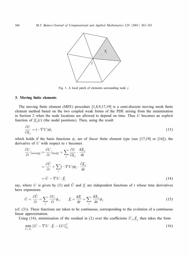
366 M.J. Baines / Journal of Computational and Applied Mathematics 128 (2001) 363–381
Fig. 1. A local patch of elements surrounding node j.
3. Moving �nite elements
The moving #nite element (MFE) procedure [1,8,9,17,19] is a semi-discrete moving mesh #niteelement method based on the two coupled weak forms of the PDE arising from the minimisationin Section 2 when the node locations are allowed to depend on time. Thus U becomes an explicitfunction of X j(t) (the nodal positions). Then, using the result
@U@X j
= (−�U )�j (13)
which holds if the basis functions �j are of linear #nite element type (see [17,19] or [16]), thederivative of U with respect to t becomes
@U@t|movingX =
@U@t|#xedX +
∑j
@U@X j· dX j
dt
=@U@t
+∑j
(−�U )�j ·@X j
dt
= U −�U · X (14)
say, where U is given by (3) and U and X are independent functions of t whose time derivativeshave expansions
U =@U@t
=∑j
@Uj@t�j; X =
dXdt
=∑j
dX j
dt�j (15)
(cf. (3)). These functions are taken to be continuous, corresponding to the evolution of a continuouslinear approximation.
Using (14), minimisation of the residual in (2) over the coe=cients U j; X j then takes the form
minU j ; X j‖U −�U · X − LU‖2L2 (16)

M.J. Baines / Journal of Computational and Applied Mathematics 128 (2001) 363–381 367
which, using (15), leads to the MFE or extended Galerkin equations
〈�j; U −�U · X − LU 〉= 0; (17)
〈(−�U )�j; U −�U · X − LU 〉= 0: (18)
The resulting ODE system may be solved by a stiE ODE package as in the method of lines.The method has been analysed in [1] and found to possess the following properties:
Property 1. For scalar #rst-order time-dependent PDEs in any number of dimensions the method isan approximate method of characteristics.
Property 2. For scalar second-order time-dependent PDEs in one dimension the method repels nodesfrom inMection points towards areas of high curvature. At steady state the nodes asymptoticallyequidistribute a power of the second derivative.
However, the method also has intrinsic singularities.
• If �U has a component whose values are equal in adjacent elements (dubbed parallelism byMiller [19]), the system of equations (17) and (18) becomes singular and must be regularised insome way (see [1,8,9,17,19]).
• If the area of an element vanishes, the system again becomes singular and special action isrequired.
Each of these singularities also leads to poor conditioning of the corresponding matrix systemsnear to singularity. For these reasons the method is usually regularised by adding penalties in thefunctional (16).
3.1. Steady state
In the same way as for #xed meshes the MFE method may in principle be used to generate weakforms for approximately solving the steady PDE Lu = 0 by driving the MFE solutions to steadystate (assuming convergence). From Property 2 of Section 3 it may be expected that for scalarsecond-order PDEs in one dimension the nodes will converge towards areas of high curvature.Property 1, however, indicates that for scalar 6rst-order PDEs the nodes continue to move withcharacteristic speeds and are not therefore expected to settle down to a steady state.
To reach a steady state we may replace the velocities U and X by explicit time discretisationswith index n and time steps �; and use the resulting equations (17) and (18) to drive Un; X n toconvergence, provided that is possible. Since we are only interested in the limit the mass matrixmay be replaced by any positive de#nite matrix. The steady-state solution satis#es the weak forms⟨(
1
−�U
)�j; LU
⟩= 0: (19)
We note that from (16) the MFE method in the steady case implements the minimisation
minU ; X‖LU‖2L2 : (20)
368 M.J. Baines / Journal of Computational and Applied Mathematics 128 (2001) 363–381
Although U and X no longer appear in LU , the minimisation is over all functions lying in the spacespanned by {�j; (−�U )�j}. In one dimension this space is also spanned by the discontinuous linearfunctions on the mesh (see [1]) (provided that Ux is not equal in adjacent elements).
3.2. The optimal property of the steady MFE equations
It has been shown in [16] that the optimal property of Section 2.2 generalises to the steady MFEequations (19). If Lu=0 can be derived from a variational principle then, as in Section 2.2, solutionsof the weak forms (19) provide a local optimum of (9) over the approximation space spanned bythe set of functions {�j; (−�U )�j}. We shall refer to this property as the optimal property. Thisresult essentially follows from (14) modi#ed to apply to variations, i.e.
�U |movingX = �U |#xedX −�U · �X : (21)
The MFE method may therefore be used as an iterative procedure to generate locally optimal meshes(see [16]). If desired, the MFE mass matrix may be replaced by any positive de#nite matrix (see[18]).
Substituting (7) into (19), the functional (9) is minimised by solutions of the two weak forms⟨�j;
@F@U
⟩+⟨��j;
@F@�U
⟩= 0; (22)
⟨�j;
@F@x
⟩+⟨��j;
(F −�U · @F
@�U
)⟩= 0; (23)
where the identity
� ·(F −�U · @F
@�U
)=@F@x
+@F@U�U −
(� · @F
@�U
)�U (24)
has been used to transform the second component of (19) into the equivalent equation (23) whichis formally suitable for piecewise linear approximation. In carrying out the integration by parts toarrive at (23) we have used the fact that the continuous piecewise linear #nite element basis function�j vanishes on the boundary of the patch.
In particular, for the least squares functional (11) the weak forms are⟨�j;
@f2
@U
⟩+
⟨��j;
@f2
@�U
⟩= 0; (25)
⟨�j;
@f2
@x
⟩+
⟨��j;
(f2 −�U · @f
2
@�U
)⟩= 0: (26)
4. Least squares �nite elements
Notwithstanding the use of the L2 norm in the construction of the Galerkin and MFE methods inSections 2 and 3, from a fully discrete point of view the procedure used there is a restricted leastsquares minimisation because it is carried out only over the velocities U j and X j. The variables Uj

M.J. Baines / Journal of Computational and Applied Mathematics 128 (2001) 363–381 369
and X j are treated as constants, independent of U j and X j and the coupling is ignored, as in themethod of lines.
A fully discrete least squares approach is feasible, however, if ut is discretised in time before theleast squares minimisations are carried out. Minimisation is then over Uj and X j rather than U j andX j and the variational equations include additional terms that do not arise in the semi-discrete #niteelement formulations.
In what follows we shall restrict attention to 6rst-order space operators Lu depending on x; u and�u only.
4.1. Least squares 6nite elements on a 6xed grid
To describe the procedure in more detail consider a one-step (explicit or implicit) time discreti-sation of Eq. (1) of the form
un+1 − unNt
= Lu∗; (27)
where ∗ may denote n or n+ 1. The #nite-dimensional approximation Un+1 at the next time step isthen generated by least squares minimisation of the residual
R∗ =Un+1 − Un
Nt− LU ∗ (28)
of (27) over the coe=cients Un+1j via
minUn+1j
‖R∗‖2L2 : (29)
In the explicit case (∗= n) the gradient of (29) with respect to Un+1j gives rise to the weak form⟨
Rn;�n+1j
Nt
⟩= 0 (30)
which is a simple time discretisation of (4).However, in the implicit case (∗= n+ 1) the gradient of (29) with respect to Un+1
j leads to⟨Rn+1;
�n+1j
Nt− @LU
n+1
@Un+1j
⟩= 0: (31)
Eq. (31) is not simply an implicit time discretisation of (4) because of the additional terms in thetest function.
4.2. Least squares moving 6nite elements (LSMFE)
Now consider minimisation of the L2 norm in (29) over the nodal coordinates X n+1j as well as the
coe=cients Un+1j . This is the approach of the recent least squares moving #nite element (LSMFE)
method [18] which was proposed partly in an attempt to overcome the di=culties which arise with#rst-order PDEs when the nodes move with characteristic speeds.
370 M.J. Baines / Journal of Computational and Applied Mathematics 128 (2001) 363–381
By analogy with (16) consider the minimisation
minUn+1j ; X n+1
j
‖R∗‖2L2 ; (32)
where R∗ is the residual
R∗ =Un+1 − Un
Nt−�U ∗ · X
n+1 − X n
Nt− LU ∗ (33)
(cf. (16)). In the explicit case (∗ = n) ‖Rn‖2L2 is quadratic in both sets of variables Un+1j ; X n+1
j andminimisation yields⟨
Rn;
(1
−�Un
)�n+1j
Nt
⟩= 0 (34)
which is a simple time discretisation of (17).In the implicit case (∗= n+ 1), on the other hand, the gradient of ‖Rn+1‖2L2 with respect to Un+1
j
gives ⟨Rn+1;
(�n+1j
Nt− X
n+1 − X n
Nt·��n+1
j − @@Un+1
jLUn+1
)⟩= 0 (35)
while that with respect to X n+1j gives (formally)⟨
Rn+1; (−�Un+1)
(�n+1j
Nt− X
n+1 − X n
Nt·��n+1
j − @@Un+1
jLUn+1
)⟩
+∮
12(Rn+1)2�n+1
j n ds= 0 (36)
using (13), where the boundary integral in (36) (which appears due to variations in the mesh) istaken over the boundaries of the elements in the patch containing node j (see Fig. 1). The unitnormal n is measured inwards.
In deriving Eqs. (35) and (36) the functions Un+1 and X n+1 appearing in the time-discretisedterms in (33) are regarded as independent variables, but the Un+1 occurring in �Un+1 and LUn+1
are functions of x and X . We have therefore used the chain rule
@LU@Uj
=@U@Uj
@LU@U
+@�U@Uj
· @LU@�U =
@LU@U
�j +@LU@�U ·��j (37)
(see (3)) when diEerentiating �Un+1 and LUn+1 to obtain (36).We shall refer to (35) and (36) as the transient LSMFE equations. These equations have been
solved in [18] in one dimension and, in spite of hopes to the contrary, the method was found tostill possess Property 1 of Section 3, that for scalar #rst-order time-dependent PDEs the method isan approximate method of characteristics. This property survives because, even though Eqs. (35)and (36) diEer from (17) and (18), approximate characteristic speeds still make the residual vanish.However, as we shall see, the method does generate the optimal property of MFE at the steady state.
M.J. Baines / Journal of Computational and Applied Mathematics 128 (2001) 363–381 371
4.3. Steady-state least squares moving 6nite elements
Consider now the steady-state limit of (35) and (36) as Nt → ∞, assuming that convergencetakes place. Since Rn+1 → LU , Eqs. (35) and (36) become⟨
LU;@@Uj
LU
⟩=
⟨LU; (−�U )
@@Uj
(LU )
⟩+∮
12(LU )2�jn ds= 0 (38)
which may be written in the equivalent forms⟨@(LU )2
@U; �j
⟩+
⟨@(LU )2
@�U ;��j⟩= 0; (39)
⟨@(LU )2
@x; �j
⟩+
⟨((LU )2 − (�U ) · @(LU )2
@�U
);��j
⟩= 0; (40)
where we have used (37) and the identity (24) with F=(LU )2. Eq. (38) may be obtained by directminimisation of ‖LU‖2L2 over Uj and X j.Referring back to (25) and (26) we see that Eqs. (39) and (40) are the steady MFE equations
for the PDE
− @(Lu)2
@u+� · @(Lu)
2
@�u = 0 (41)
(see [16]) which corresponds to the Euler–Lagrange equation for the minimisation of the least squaresfunctional ‖Lu‖2L2 .
To solve the nonlinear equations (39) and (40) by iteration we may use the correspondingtime-stepping method, (35) and (36), with n as the iteration parameter, or any other convenientiteration (see Section 7).
4.4. Properties of the steady LSMFE equations
(i) As we have already seen in Section 3:3, for steady problems the least squares functionalF(x; U;�U ) = (LU )2 leads to the weak forms (25) and (26) and therefore (39) and (40), and wehave the optimal property, as expected.
(ii) In the LSMFE tests carried out in [18] on scalar #rst-order steady-state equations it is shownthat the nodes no longer move with characteristic speeds, as in Property 1 of Section 3, but insteadmove to regions of high curvature as in Property 2. This is a useful property and could have beenexpected because the least squares procedure in eEect embeds the original #rst-order equation inthe second-order Eq. (41) for which the MFE steady limit yields the asymptotic equidistribution ofProperty 2 of Section 3.1.
(iii) In the particular case where LU takes the form of a divergence of a continuous function ofU , we may apply an extension of the result in [4] which shows that, asymptotically, minimisationof ‖LU‖2L2 is equivalent to equidistribution of LU over all the elements in a certain sense. Thus forexample in the case where
Lu=� · (au) (42)
372 M.J. Baines / Journal of Computational and Applied Mathematics 128 (2001) 363–381
with constant a, the LSMFE method asymptotically equidistributes the piecewise constant residualLU =� · (aU ) in each element in the sense described in Section 6.1.We now give some illustrative examples of steady LSMFE.
4.5. Examples
(i) Take
Lu= u− f(x) (43)
for which the steady LSMFE weak forms, from (39) and (40), are⟨(1
−�U
)�j; (U − f(x))
⟩= 0; (44)
subject to boundary conditions, which provide a local minimum for the least squares variable nodeapproximation problem
minUj;X j
∫(U − f(x))2 dx: (45)
(Superior results for this problem can however be obtained by considering piecewise linear discon-tinuous approximation — see Section 4.6.)
(ii) Take
Lu= a ·�u= a@u@x
+ b@u@y; (46)
where a= (a; b) is constant. In this case Eq. (41) becomes the degenerate elliptic equation
� · ((a ·�u)a) =(a@@x
+ b@@y
)(a@u@x
+ b@u@y
)= 0: (47)
The steady LSMFE weak forms, from (39) and (40), are
〈a ·�U; a ·��j)〉= 0 (48)
and ⟨�j; (a ·�U )
@(a ·�U )@x
⟩− 1
2〈��j; (a ·�U )2〉= 0; (49)
subject to boundary conditions, which provide a local minimum for the least squares variable nodeapproximation problem
minUj;Xj
∫(a ·�U )2 dx (50)
(see ([2,21])). These are also the steady MFE equations for the second-order degenerate ellipticequation
� · ((a ·�u)a) = 0: (51)
If a depends on x but is continuous and divergence-free, then LU = a · �U is the divergence ofa continuous function and this example has the asymptotic equidistribution property referred to in

M.J. Baines / Journal of Computational and Applied Mathematics 128 (2001) 363–381 373
Section 4.4, in this case asymptotically equidistributing Pa · �U where Pa consists of the elementaverages of a(x).
(iii) Take
Lu= |�u|=((
@u@x
)2+(@u@y
)2)1=2(52)
for which Eq. (41) is Laplace’s equation
�2u= 0: (53)
The steady LSMFE weak forms, from (39) and (40), are
〈��j;�U 〉=⟨�j;
@(�U )2
@X
⟩− 〈��j; (�U )2〉= 0; (54)
subject to boundary conditions, which provide a minimum for the variable node Dirichlet problem(see e.g. [22])
minUj;X j
∫|�U |2 dx: (55)
4.6. The MBF approach
If the functional F is independent of �U (the best approximation problem) we may take combi-nations of the variations �Uj and �X j to design simpler sequential algorithms. The #rst variation ofthe square of the L2 norm of R= LU , using (32), (35), (36) and (38), gives
� 12‖LU‖
2L2=⟨LU;
@LU@U
�j
⟩(�Uj −�U · �X j) (56)
−∮
12(LU )2�jn · �X j ds: (57)
Setting �X j = 0 gives the #xed mesh least squares equation
〈LU @LU@U
; �j〉= 0 (58)
while, setting
�Uj −�U · �X j = 0
gives ∮12(LU )2�jn ds= 0; (59)
an equation for updating the nodes locally which depends only on the integral over the boundariesof the patch containing node j. The constraint (4:6), which forces �Uj to vary with �X j, correspondsto linear interpolation/extrapolation on the current piecewise linear U function. This approach, whichdepends only on local problems, is called the moving best #ts (MBF) method in [1] and is the basisof best approximation algorithms in [2,21].
374 M.J. Baines / Journal of Computational and Applied Mathematics 128 (2001) 363–381
5. Finite volume methods
We turn now to a discussion of the use of discrete l2 norms with area weighting as a basis forgenerating #nite volume schemes, to a large part the result of a simple quadrature applied to the L2norm used previously.
De#ne the discrete l2 norm as the weighted sum over triangles of the average residual of thePDE, viz.
‖R‖2l2 =∑T
ST PR2T (60)
(cf. (2), (16), (29) and (32)), where the su=x T runs over all the triangles of the region, ST is thearea of triangle T and PRT is the average value of the residual R over the vertices of T .This norm coincides with the L2 norm in the case where R is constant on each triangle. For then
‖R‖2L2 =∫R2 dx =
∑T
∫TR2 dx =
∑T
PR2T
∫Tdx =
∑T
ST PR2T = ‖R‖2l2 (61)
as in example (ii) of Section 4.5 where R = LU = a · �U , the advection speed a being constantand U piecewise linear. If the area weighting in (60) is omitted this link is lost. However, oneobjection to the use of least squares residuals is that when triangles become degenerate the norm ofthe derivative is unbounded. By rede#ning the norm in (60) with a squared weight S2T instead of STthe norm is always well de#ned and still has an approximate equidistribution property (see [19]).Here we concentrate on (60); however, the modi#cations are straightforward.
The form (60) may be rewritten as a sum over nodes j, namely
‖R‖2l2 =13
∑j
∑{Tj}
STj PR2Tj ; (62)
where {Tj} runs over the patch of triangles abutting node j (see Fig. 1).We may take (�U )T to be the gradient associated with the linearly interpolated corner values of
U in the triangle T , given by (see [16])
(�U )T =
(−∑i UiNYi∑i XiNYi
;∑i UiNXi−∑i YiNXi
)=
(∑i YiNUi∑i XiNYi;−∑i XiNUi∑i YiNXi
); (63)
where the sums run over the corners i of the triangle T and NXi;NYi;NUi denote the incrementsin the values of X; Y; U taken anticlockwise across the side of T opposite the corner concerned (seeFig. 1). This is of course identical to the #nite element gradient with piecewise linear approximation.In the same notation the area of the triangle T is
ST =12
∑i
XiNYi =−12
∑i
YiNXi (64)
which incorporates a summation by parts.
M.J. Baines / Journal of Computational and Applied Mathematics 128 (2001) 363–381 375
5.1. Moving 6nite volumes
By analogy with the MFE method of Section 3 a moving #nite volume (MFV) method may beset up by minimising the residual
‖U −�U · X − LU‖l2 (65)
(see (60)) over U j and X j, which leads to∑{Tj}
STj(U −�U · X − LU )j = 0; (66)
∑{Tj}
STj(U −�U · X − LU )j(−�U )Tj = 0 (67)
(cf. (17) and (18)) where {Tj} is the set of triangles abutting node j and the su=x j indicatesthat terms involving U and X are evaluated at the node j while those involving �U and LU areevaluated over the triangle Tj.
Property 1 of Section 3 still holds since the residual vanishes as before when X approximates char-acteristic speeds. The method also has the same singularities as MFE, in particular when componentsof the gradients �U are the same in adjacent elements.
At the steady state we have the steady MFV equations∑{Tj}
STj(LU )j = 0; (68)
∑{Tj}
STj(LU )T (−�U )Tj = 0: (69)
If Lu is derived from a variational principle, given by (7), these become∑{Tj}
STj
(− @F@U
+� · @F@�U
)j= 0; (70)
∑{Tj}
STj
(− @F@U
+� · @F@�U
)j(−�U )Tj = 0 (71)
which, using the summation by parts implicit in (64), lead to∑{Tj}
STj
(− @F@U− 1
2@F@�U · nj
)j= 0; (72)
∑{Tj}
STj
(− @F@U− 1
2@F@�U · nj
)j(−�U )Tj = 0; (73)
where nj = (NYj;−NXj) is the inward normal to the side opposite node j scaled to the length ofthat side (see [5] and Fig. 1).

376 M.J. Baines / Journal of Computational and Applied Mathematics 128 (2001) 363–381
5.2. A discrete optimisation
By analogy with (60) a discrete form of (9) is
Id(F) =∑T
STF(X ;U;�U )T =∑T
ST13
3∑i=1
F(X i; Ui; (�U )T ); (74)
where the overbar denotes the average value over the vertices of T . (When Euler #rst derived hisvariational equation he used such a #nite form, although on a #xed mesh of course.)
The sum in (74) may be rewritten as a sum over nodes j as
Id(F) =13
∑j
∑{Tj}
STj13
3∑i=1
F(X i; Ui; (�U )Tj); (75)
where i runs over the corners of the triangle Tj.A moving mesh method may be derived based on the two coupled equations which arise when
(75) is optimised over both Uj and X j. DiEerentiating (75) with respect to Uj gives
@Id@Uj
=∑{Tj}
STj13
(@F@U
+@F@�U ·
@�U@U
)j
(76)
leading to the equation∑{Tj}
(ST@F@U
+12@F@�U · n
)j= 0: (77)
This is a #nite volume weak form which corresponds to the #nite element weak form (10). It isalso identical to (72) showing that the optimal property of Section 2.2 goes over to the steady-state#nite volume case when Uj varies.
DiEerentiating with respect to X j gives
@Id@X j
=∑{Tj}
STj13
(@F@X
+@�U@X
· @F@�U
)j
(78)
which leads to∑{Tj}
(ST@F@X−(NU
(0 −11 0
)− 1
2S−1T �UT · n
)@F@�U
)j
= 0 (79)
(cf. (73)). Eq. (79) is the companion weak form to (73), corresponding to the second #nite elementweak form (23). However, this diEers considerably from (23) showing that the optimal propertyof MFE does not go over to steady state MFV when X varies. This is because diEerentiation ofa quadrature rule with respect to X is not the same as quadrature of the derivative. In fact, it isEqs. (77) and (79) which give the optimal property.
If F = 12(LU )2, Eqs. (77) and (79) can be made the basis of a least squares method (LSMFV)
for steady problems associated with the PDE (41) with ut = 0. From (77) and (79) we have∑{Tj}
STj
(LU
@LU@U
+12LU
@LU@�U n
)j= 0 (80)
M.J. Baines / Journal of Computational and Applied Mathematics 128 (2001) 363–381 377
and∑{Tj}
[STLU −
(NU
(0 −11 0
)− 1
2S−1T �Un
)LU
@U@�U
]j
= 0: (81)
6. Time-dependent least squares moving �nite volumes
As in Section 4, a fully discrete least squares #nite volume method for time-dependent problemsis obtained if ut is discretised in time before the l2 least squares minimisations are carried out.Minimisation is over Uj and X j rather than U j and X j.Consider again the one-step time discretisation of Eq. (1) in the form (27). Then on a moving
mesh the solution at the next time step may be generated by the least squares minimisation of theimplicit form of the residual over Un+1
j and X n+1j via
minUn+1j ; X n+1
j
‖Rn+1‖2l2 ; (82)
where (cf. (60))
Rn+1 =Un+1 − Un
Nt−�Un+1 · X
n+1 − X n
Nt− LUn+1 (83)
(with �Un+1 de#ned as in (63)) and
‖R‖2l2 = 〈R; R〉l2 ; 〈P;Q〉l2 =∑{Tj}
ST PPT PQT : (84)
Setting the gradients with respect to Un+1j and X n+1
j to zero gives⟨Rn+1;
@Rn+1
@Un+1j
⟩l2
= 0 (85)
and ⟨Rn+1;
@Rn+1
@X n+1j
⟩l2
+12
∑{Tj}
(Rn+1Tj )2
@Sn+1Tj
@X n+1j
= 0: (86)
We shall refer to (85) and (86) as the transient LSMFV method. For scalar #rst-order time-dependentPDEs the method is still an approximate method of characteristics since approximate characteristicspeeds always make the residual Rn+1 vanish. However, in the steady state it has other features.
6.1. Steady-state least squares 6nite volumes
Consider now the steady limit. Then from (82) we are minimising ‖LU‖2l2 and (85) and (86)reduce to⟨
LU;@(LU )@Uj
⟩l2
= 0 (87)
378 M.J. Baines / Journal of Computational and Applied Mathematics 128 (2001) 363–381
and ⟨LU;
@LU@X j
⟩l2
+12
∑Tj
(LU )2Tj
@STj@X j
= 0 (88)
which are identical to (80) and (81) (see [5,20]).It has been shown in [4] that if LU is the divergence of a continuous function, then the optimal
values of LU are equidistributed in the sense that the double sum over elements∑e
∑e′
(SeLUe − Se′LUe′)2 (89)
is minimised. Thus if Lu= a ·�u with constant a, as in example (ii) of Section 4.5 the piecewiseconstant LU = a · �U is equidistributed over the elements in this sense. The same result is onlyasymptotically true for the LSMFE method (see Section 4.4).
6.2. Example
Consider again example (ii) of Section 4.5, for which the steady-state residual is
LU = a ·�U: (90)
Then (85) and (86) reduce to⟨LU; a · @(�U )
@Uj
⟩l2
=
⟨LU;
@(a ·�U )@X j
⟩l2
+12
∑Tj
(LUT )2@STj@X j
= 0; (91)
subject to boundary conditions, where from (63)
@(a ·�U )Tj@X j
=NUj
(−ba
)− 1
2S−1Tj (a ·�U )Tjnj: (92)
Recall that nj is the inward normal to the side of the triangle opposite j scaled by the length of thatside and NUj is the increment in U across that side, taken anticlockwise.Eq. (91) may be written∑
Tj
(a ·�U )Tj(a · nj) = 0 (93)
and ∑Tj
[(a ·�U )T NU
(−ba
)− 1
2(a ·�U )2Tn
]j
= 0: (94)
We observe that (93) is identical to (48), noting that �U is constant and �� = S−1T n. However,
(94) does not correspond to (49), even when a is constant, so the two methods are not identicalunder node movement.
7. Minimisation techniques
The fully discrete least squares methods of Sections 4 and 6, unlike the unsteady Galerkin methodsof Sections 2 and 3, provide a functional to reduce and monitor. It is therefore possible to take an

M.J. Baines / Journal of Computational and Applied Mathematics 128 (2001) 363–381 379
optimisation approach to the generation of a local minimum. Note that the time-stepping methodsdiscussed earlier do not necessarily reduce the functional.
Descent methods are based upon the property that the #rst variation of a functional F,
�F=@F@Y
= g T�Y (95)
say, is negative when
�Y =−�g=−�@F@Y
; (96)
where � is a su=ciently small positive relaxation parameter. For the present application the gradientsg have already been evaluated in earlier sections. For example, in the LSMFE method the gradientsg with respect to Uj and X j appear on the left-hand side of (35) and (36). Thus, writing Y={Y j}={Uj; X j} and g= {g
j} the steepest descent method applied to (32) with ∗= n+ 1 is
(Y n+1j )k+1 − (Y n+1
j )k =− �kj (g n+1j
)k (97)
(k = 1; 2; : : :) where �kj is the relaxation parameter. Choice of �kj is normally governed by a linesearch or a local quadratic model.
The left-hand side of (97) may be preconditioned by any positive de#nite matrix. The Hessiangives the full Newton method but may be approximated in various ways. In [18] a positive de#niteregularising matrix is used in place of the Hessian to generate the solution.
In the present application a local approach may be followed which consists of updating theunknowns one node at a time, using only local information. For a given j each step of the form(97) reduces the functional (32), even when the other Y n+1 values are kept constant. The updatesmay be carried out in a block (Jacobi iteration) or sequentially (Gauss–Seidel). A variation on thelocal approach is to update Uj and X j sequentially, which gives greater control of the mesh. Descentmethods of this type have been used by Tourigny and Baines [21] and Tourigny and Hulsemann[22] in the L2 case and by Roe [20] and Baines and Leary [5] in the l2 case.
8. Conclusions
We conclude with a summary of the main results.
• The MFE method is a Galerkin method extended to include node movement. Its main propertiesare:(a) numerical imitation of the method of characteristics for #rst-order equations in any number
of dimensions;(b) repulsion of nodes from inMection points for second-order equations in one dimension;(c) for
Lu=− @F@u
+� · @F@�u = 0 (98)
380 M.J. Baines / Journal of Computational and Applied Mathematics 128 (2001) 363–381
the steady MFE equations provide a local optimum for the variational problem
minUj;X j
∫F(x; U;�U ) dx (99)
in a piecewise linear approximation space with moving nodes.• The implicit semi-discrete in time least squares method (LSMFE) is a least squares method
extended to include node movement. It diEers from MFE through more complicated test functionsand the extra term found in (36), although in the case of #rst-order equations it shares with MFEthe property of being a numerical method of characteristics. However, in the steady state theLSMFE equations for Lu= 0 are equivalent to the steady MFE weak forms for the PDE
− @ (Lu)2
@u+� ·
(@ (Lu)2
@�tu
)= 0 (100)
and therefore provide a local minimum for the variational problem
minUj;X j
∫(LU )2 dx: (101)
Moreover, it can be shown that, if LU is the divergence of a continuous Mux function then theMux across element boundaries is asymptotically equidistributed over the elements.• The LSMFV method is a moving mesh method based on minimisation of a weighted l2 normof the residual of the semi-discrete in time PDE over the solution and the mesh. It shares withLSMFE the property of generating approximate characteristic speeds. At steady state, however,it lacks the optimal property of LSMFE but it has the more precise property that, if LU is thedivergence of a continuous Mux function, then the Mux across element boundaries is equidistributeddiscretely (not just asymptotically) over the elements in the sense of (89) [4].
• Solutions may be obtained by the minimisation procedures of optimisation theory applied to theappropriate norm. A local approach to optimisation is advantageous in preserving the integrity ofthe mesh.
The MFE, LSMFE and LSMFV methods have been shown to be eEective in generating approximatesolutions to scalar diEerential problems in multi-dimensions which exhibit shocks and contact dis-continuities [1,2,5,6,8,9,16,20]. The MFE and LSMFV methods have also been eEective in obtainingapproximate solutions of systems of equations [1,5,6,8,9].
Finite volume methods of the type discussed here do not give highly accurate solutions on coarsemeshes. However, high accuracy is not crucial as far as the mesh is concerned. Thus it may beargued that an LSMFV method is su=ciently accurate for the mesh locations but a more sophisticatedmethod which is robust on distorted meshes, such as high-order #nite elements or multidimensionalupwinding [11,15], may be required for the solution on the optimal mesh.
An outstanding problem is how to avoid the generation of characteristic speeds by the MFE andMFV methods for #rst-order equations. In the case of MFE a clue may be found in the LSMFEmethod, which embeds the original #rst-order equation in a second-order degenerate elliptic equationprior to moving the nodes. When solved by a relaxation method in an iterative manner, in eEectapplying a #nite diEerence scheme to the associated parabolic equation, the resulting nodal speedsare not characteristic but instead move nodes from low-curvature regions to high-curvature regions,as required. Moreover, the nodes tend to align themselves with characteristic curves, although they

M.J. Baines / Journal of Computational and Applied Mathematics 128 (2001) 363–381 381
do not actually move along them. Although the resulting nodal speeds are eEective in this sense,the LSMFE does not generate the correct solution to the #rst-order equation since it has now beenembedded a second-order equation. Thus, if these speeds are to be used it is impossible for thediscrete equations to be set up from a uni#ed approach. Instead it is necessary to generate thespeeds from the LSMFE method which must then be substituted into the Lagrangian form of the#rst-order equation, to be solved separately using any convenient method.
References
[1] M.J. Baines, Moving Finite Elements, Oxford University Press, Oxford, 1994.[2] M.J. Baines, Algorithms for optimal discontinuous piecewise linear and constant L2 #ts to continuous functions with
adjustable nodes in one and two dimensions, Math. Comp. 62 (1994) 645–669.[3] M.J. Baines, Grid adaptation via node movement, Appl. Numer. Math. 26 (1998) 77–96.[4] M.J. Baines, Least squares and equidistribution in multidimensions, Numer. Methods Partial DiEerential Equations
15 (1999) 605–615.[5] M.J. Baines, S.J. Leary, Fluctuations and signals for scalar hyperbolic equations on adjustable meshes, Numerical
Analysis Report 6=98, Department of Mathematics, University of Reading, 1999. Comm. Numer. Methods Eng. 15(1999) 877–886.
[6] M.J. Baines, S.J. Leary, M.E. Hubbard, A #nite volume method for steady hyperbolic equations with mesh movement,in: Vilsmeier, Benkhaldoun, Hanel (Eds.), Proceedings of Conference on Finite Volumes for Complex ApplicationsII, Hermes, Paris, 1999, pp. 787–794.
[7] C. Budd et al., Self-similar numerical solutions of the porous-medium equation using moving mesh methods, Philos.Trans. Roy. Soc. London A 357 (1999) 1047–1077.
[8] N.N. Carlson, K. Miller, Design and application of a gradient weighted moving #nite element method I: in onedimension, SIAM J. Sci. Comput. 19 (1998) 728–765.
[9] N.N. Carlson, K. Miller, Design and application of a gradient weighted moving #nite element method II: in twodimensions, SIAM J. Sci. Comput. 19 (1998) 766–798.
[10] C. de Boor, A Practical Guide to Splines, Springer, New York, 1978.[11] H. Deconinck, P.L. Roe, R. Struijs, A multidimensional generalisation of Roe’s Mux diEerence splitter for the Euler
equations, Comput. Fluids 22 (1993) 215.[12] M. Delfour et al., An optimal triangulation for second order elliptic problems, Comput. Methods Appl. Mech. Eng.
50 (1985) 231–261.[13] E.A. Dor#, L.O’C. Drury, Simple adaptive grids for 1D initial value problems, J. Comput. Phys. 69 (1987) 175–195.[14] W. Huang et al., Moving mesh partial diEerential equations, SIAM J. Numer. Anal. 31 (1994) 709–730.[15] M.E. Hubbard, P.L. Roe, Compact high-resolution algorithms for time-dependent advection on unstructured grids,
Internat. J. Numer. Methods Fluids (1999) 33 (2000) 711–736.[16] P.K. Jimack, Local minimisation of errors and residuals using the moving #nite element method. University of Leeds
Report 98.17, School of Computer Science, 1998.[17] K. Miller, Moving #nite elements II, SIAM J. Numer. Anal. 18 (1981) 1033–1057.[18] K. Miller, M.J. Baines, Least squares moving #nite elements. OUCL Report 98=06, Oxford University Computing
Laboratory, 1998. IMA J. Numer. Anal., submitted.[19] K. Miller, R.N. Miller, Moving #nite elements I, SIAM J. Numer. Anal. 18 (1981) 1019–1032.[20] P.L. Roe, Compounded of many simples, In: Ventakrishnan, Salas, Chakravarthy (Eds.), Challenges in Computational
Fluid Dynamics, Kluwer, Dordrecht, 1998, pp. 241–258.[21] Y. Tourigny, M.J. Baines, Analysis of an algorithm for generating locally optimal meshes for L2 approximation by
discontinuous piecewise polynomials, Math. Comp. 66 (1997) 623–650.[22] Y. Tourigny, F. Hulsemann, A new moving mesh algorithm for the #nite element solution of variational problems,
SIAM J. Numer. Anal. 34 (1998) 1416–1438.
Journal of Computational and Applied Mathematics 128 (2001) 383–398www.elsevier.nl/locate/cam
Adaptive mesh movement — the MMPDE approach and itsapplications
Weizhang Huanga ; 1, Robert D. Russellb; ∗; 2aDepartment of Mathematics, The University of Kansas, Lawrence, KS 66045, USA
bDepartment of Mathematics and Statistics, Simon Fraser University, Burnaby BC, Canada V5A 1S6
Received 25 January 2000
Abstract
A class of moving mesh algorithms based upon a so-called moving mesh partial di0erential equation (MMPDE) isreviewed. Various forms for the MMPDE are presented for both the simple one- and the higher-dimensional cases.Additional practical features such as mesh movement on the boundary, selection of the monitor function, and smoothingof the monitor function are addressed. The overall discretization and solution procedure, including for unstructured meshes,are brie4y covered. Finally, we discuss some physical applications suitable for MMPDE techniques and some challengesfacing MMPDE methods in the future. c© 2001 Elsevier Science B.V. All rights reserved.
Keywords: Moving mesh algorithm; MMPDE
1. Introduction
In this paper we discuss a class of adaptive mesh algorithms for solving time-dependent partialdi0erential equations (PDEs) whose solutions are characterized largely by varying behavior over agiven physical domain. In particular, we consider a class of moving mesh methods which employa moving mesh partial di0erential equation, or MMPDE, to perform mesh adaption in such a waythat the mesh is moved around in an orderly fashion.
The MMPDE is formulated in terms of a coordinate transformation or mapping. For a mappingmethod, mesh generation is considered to be mathematically equivalent to determining a coordinatetransformation from the physical domain into a computational domain. More speci:cally, let �⊆R3
be the physical domain on which the physical problem is de:ned, and let �c⊆R3 be the compu-tational domain chosen somewhat arti:cially for the purpose of mesh adaption. Denote coordinates
∗ Corresponding author.E-mail address: [email protected] (R.D. Russell).1 The author was supported in part by the NSF (USA) Grant DMS-9626107.2 The author was supported in part by NSERC (Canada) Grant OGP-0008781.
0377-0427/01/$ - see front matter c© 2001 Elsevier Science B.V. All rights reserved.PII: S 0377-0427(00)00520-3
384 W. Huang, R.D. Russell / Journal of Computational and Applied Mathematics 128 (2001) 383–398
in � and �c by x = (x1; x2; x3)T and � = (�1; �2; �3)T, respectively. The idea behind mapping meshmethods is to generate meshes on � as images of a reference mesh on �c through a one-to-onecoordinate transformation, say x = x(�) : �c → �. It is common to de:ne such a mapping throughthe so-called variational approach, i.e., to determine the mapping as the minimizer of a functionalinvolving various properties of the mesh and the physical solution, e.g., see [33,40] and referencestherein. Mapping methods have traditionally been used for the generation of structured meshes, butmore recently Cao et al. [13] have demonstrated how a mapping method can naturally be used forunstructured mesh generation and adaption as well.
A variety of variational methods have been developed in the past [33,40], some of the mostsuccessful being those in [41,6,22]. The mesh generation system used in [41] consists of two variablecoeHcient di0usion equations (the Euler–Lagrange equations for a simple functional, as we discussbelow). Winslow’s method is generalized in [6] by including mesh properties such as concentration,smoothness, and orthogonality into the mesh adaption functional. The method is extended further byBrackbill [5], who includes directional control. The method introduced in [22] de:nes the coordinatetransformation as a harmonic mapping which is the extremal of a so-called action functional or energyintegral. Closely related methods de:ne the coordinate transformation in terms of an elliptic system,e.g., the Euler–Lagrange equations for the variational form. Indeed, the mesh generation methodproposed in [39], which consists of solving two Poisson equations with control source terms, canbe regarded as being of this form. As well, the Soviet literature is also replete with papers onadaptive methods for generating the mesh through a coordinate transformation, e.g. see the work in[24,42,34].
It is interesting to note that in order to avoid potential mesh crossings or foldings most of themesh adaption functionals are formulated in terms of the inverse mapping � = �(x) instead ofx = x(�) (e.g., see the discussion in [22]). A mesh partial di0erential equation is then obtainedfor � as the Euler–Lagrange equation for the functional. Often this is then transformed into anequation for x(�) by interchanging the roles of dependent and independent variables. The mesh is:nally obtained by numerically solving this MPDE on a given computational mesh. It is necessaryto interpret the physical PDE and MMPDE in both the physical and computational variables, andmoreover, to do so in such a way that key properties of the transformed PDEs such as conservationare properly treated. In Section 2 we present the relevant transformation relations between the twosets of variables.
In Section 3 we present the basic MMPDEs. In the 1D (one space dimensional) case, a suHcientvariety of them has been introduced within our general framework so as to incorporate virtuallyall the 1D moving mesh methods which have been used heretofore [27,28]. In higher dimensions,we use a gradient 4ow equation which arises from the variational form. A distinguishing feature ofthe MMPDE approach from any other moving mesh approaches is that it uses a parabolic PDE formesh movement. In addition to the basic formulation, we discuss the issue of how to deal with theboundary and how to choose the monitor function for solution adaptivity.
In Section 4, the crucial issues of how to discretize the PDEs and solve the coupled systemfor the coordinate transformation and physical solution are discussed. The way in which this isextended to the unstructured mesh case is treated in Section 5. Numerical application areas whichillustrate the general usefulness of the MMPDE approach are discussed in Section 6. Lastly, inSection 7 we give some conclusions and mention some outstanding issues requiring further investi-gation.
W. Huang, R.D. Russell / Journal of Computational and Applied Mathematics 128 (2001) 383–398 385
2. Transformation relations
Transformation relations play an essential role for the MMPDE mesh method and for other methodsbased on coordinate transformations. They constitute the necessary tools in use for transformingphysical PDEs between physical and computational domains and formulating mesh equations. Herewe derive the relations needed in this paper and refer the interested reader to [40] for a morecomplete list of transformation relations and their derivations.
Consider a time-dependent (invertible) coordinate transformation x= x(�; t) : �c → � and denoteits inverse by �= �(x; t). The covariant and contravariant base vectors are de:ned by
ai =@x@�i
; ai =��i; i = 1; 2; 3; (1)
where � is the gradient operator with respect to x. The Jacobian matrix J of the coordinate trans-formation and its inverse J can then be expressed as
J ≡ @(x1; x2; x3)@(�1; �2; �3)
= [a1; a2; a3]; J ≡ @(�1; �2; �3)@(x1; x2; x3)
=
(a
1)T
(a2)T
(a3)T
: (2)
Noticing that
J−1 =1J[cofactor(J)]T =
1J[a2 × a3; a3 × a1; a1 × a2]
T; (3)
where J = det(J) = a1 · (a2 × a3) is the Jacobian (determinant), the chain rule JJ = I leads to therelations
ai =1Jaj × ak ; ai = Jaj × ak ; aial = �l
i ; (i; j; k) cyclic; (4)
where �li is the Kronecker delta function.
It is easy to verify that
∑i
@@�i
(Jai) = 0: (5)
This identity is important because it must be used when interchanging the conservative and non-conservative forms of many formulas.
For an arbitrary function u= u(x; t), we denote its counterpart in the new coordinate set (�; t) byu, i.e., u = u(x(�; t); t). Then, the gradient operator takes the forms in �
� =∑
i
ai @@�i
(non-conservative form);
=1J
∑i
@@�i
Jai (conservative form); (6)
386 W. Huang, R.D. Russell / Journal of Computational and Applied Mathematics 128 (2001) 383–398
which follow from
�u=[
@u@(x1; x2; x3)
]T
=
[@u
@(�1; �2; �3)· @(�
1; �2; �3)@(x1; x2; x3)
]T
=
[@(�1; �2; �3)@(x1; x2; x3)
]T·[
@u@(�1; �2; �3)
]T
=∑
i
ai @u@�i
and from identity (5).The identity
Jt = J� · xt (7)
follows from the fact that
Jt =∑
i
@ai
@t· (aj × ak) (i; j; k) cyclic
= J∑
i
ai · @ai
@t
= J∑
i
ai · @xt
@�i:
Eq. (7) is frequently referred to [38] as the geometric conservation law (GCL). It relates the changerate of the volume of a cell to its surface movement.
Di0erentiating u(�; t) = u(x(�; t); t) with respect to t while :xing � and using (7) gives
ut = u t −�u · xt (non-conservative form);
Jut = (J u)t − J� · (uxt) (conservative form):(8)
Thus far, the transformation relations have been given in three dimensions. The correspondingtwo-dimensional forms can be obtained from these formulas by simply setting the third base vectorsto be the unit vector, a3 = a3 = (0; 0; 1)T, and dropping the third component from the :nal results.For instance, if we denote the two-dimensional physical and computational coordinates by x=(x; y)T
and �= (�; �)T, and the base vectors by
a1 =
[x�
y�
]; a2 =
[x�
y�
]; a1 =
[�x
�y
]; a2 =
[�x
�y
]; (9)

W. Huang, R.D. Russell / Journal of Computational and Applied Mathematics 128 (2001) 383–398 387
we have
J = det
x� x� 0
y� y� 0
∗ ∗ 1
= x�y� − x�y� (10)
and
a1 =1Ja2 × a3
=1J(x�i + y� j + ∗k)× k
=1J(−x� j + y�i + 0k)
=1J
[y�
−x�
]: (11)
Similarly, we have
a2 =1J
[−y�
x�
]: (12)
We conclude this section with an illustration of how the above relations are used in practice.Consider a di0usion–convection equation in the conservative form
ut +� · f =� · (a�u); in �; (13)
where f = f (u; x; t) and a = a(x; t)¿�¿ 0 are given functions. We want to transform it from thephysical domain to the computational domain.
Upon replacing the inner and outer gradient operators by the non-conservative and conservativeforms, respectively, the di0usion term has the conservative form
� · (a�u) =1J
∑i; j
@@�j
(aJai · aj @u
@�i
): (14)
Expanding the outer di0erentiation, using (5) and noticing that �2�i =∑
j aj · @ai=@�j, we obtain
� · (a�u) =∑i; j
(ai · aj)@
@�j
(a@u@�i
)+ a
∑i
(�2�i)@u@�i
: (15)
To :nd the expressions for �2�i; i = 1; 2; 3, we consider (15) with a = 1 and x replacing u. Thisresults in
0 =∑i; j
(ai · aj)@2x
@�i@�j+∑
i
(�2�i)ai : (16)
Taking the inner product of the above equation with al and using ai · al = �li leads to
�2�l =−∑i; j
(ai · aj)
(al · @2x
@�i@�j
): (17)
388 W. Huang, R.D. Russell / Journal of Computational and Applied Mathematics 128 (2001) 383–398
The convection term is transformed into
� · f =1J
∑i
@@�i
(Jai · f ) =∑
i
ai · @f@�i
: (18)
Substituting (8), (14), (15), and (18) into (13), we obtain the transformed equation in the conser-vative form
(J u)t +∑
i
@@�i
[Jai · ( f − uxt)] =∑i; j
@@�j
(aJai · aj @u
@�i
)(19)
or in nonconservative form
u t +∑
i
ai ·(
@f@�i− @u
@�ixt
)=∑i; j
(ai · aj)@
@�j
(a@u@�i
)+ a
∑i
(�2�i)@u@�i
: (20)
Note that we have derived (20) from a conservative equation and kept the convective 4ux f in thedivergence form (@f )=(@�i). For this reason, Hindman [25] calls (20) the chain rule conservativelaw form (CRCLF). He also shows that (20) is able to catch shock waves.
3. Formulation of MMPDEs
For a moving mesh method, the mesh points move continuously in the space–time domain andconcentrate in regions where the physical solution varies signi:cantly. An explicit rule, called amoving mesh equation, is designed to move the mesh around. It is often very diHcult to formulatea moving mesh strategy which can eHciently perform the mesh adaption while moving the meshin an orderly fashion. In principle, the mesh equation should be designed based directly on sometype of error estimates, but unfortunately, such methods often result in singular meshes due to pointscrossing and tangling.
We consider in this section, the MMPDE approach for formulating mesh equations. The basicstrategy is to de:ne the mesh equation as a time-dependent PDE based on the equidistributionprinciple or its higher-dimensional generalization. Although in the higher-dimensional case, it isusually unclear whether or not this generalization relates directly to any type of error estimates, ithas proven to perform mesh adaption well and generate nondegenerate meshes.
3.1. 1D MMPDEs
MMPDEs are :rst introduced in [27,28] as time regularizations [2] of the di0erential form of the(steady-state) equidistribution principle [19]. If g=g(x)¿ 0 is the one-dimensional monitor functionwhich controls the mesh point distribution (see below for more discussion on monitor functions),then the di0erential form of the equidistribution principle can be written in terms of the inversemapping �= �(x) as
ddx
(1gd�dx
)= 0: (21)
W. Huang, R.D. Russell / Journal of Computational and Applied Mathematics 128 (2001) 383–398 389
(For simplicity, we assume here that both the physical and computational domains are the unitinterval (0,1).) The mesh equation for the mapping x = x(�) can be obtained by interchanging theroles of dependent and independent variables in (21), namely,
dd�
(gdxd�
)= 0: (22)
The MMPDEs are de:ned by adding a time derivative (or time regularization) to (22). Three popularchoices are the MMPDEs
MMPDE4:@@�
(g@xt
@�
)=−1
�@@�
(g@x@�
); (23)
MMPDE5: xt =1�
@@�
(g@x@�
); (24)
MMPDE6:@2xt
@�2=−1
�@@�
(g@x@�
); (25)
where �¿ 0 is a parameter used for adjusting the time scale of the mesh movement. These MMPDEsare analyzed numerically and theoretically in [27,28]. Their smoothed versions are discussed in [29].
The equidistribution relation (21) can also be interpreted as the Euler–Lagrange equation for thefunctional
I [�] =12
∫ 1
0
1g
(d�dx
)2dx; (26)
and MMPDEs can be derived using this alternative form. For example, we can de:ne an MMPDEas a modi:ed gradient 4ow equation for the functional I [�], i.e.,
@�@t
=1�g
@@x
(1g@�@x
): (27)
Switching the roles of dependent and independent variables, (27) becomes
xt =1
�g3x2�
@@�
(g@x@�
); (28)
which is basically MMPDE5 with a spatially varying time scaling parameter �g3x2�.
3.2. Higher-dimensional MMPDEs
The strategy for formulating (27) is used in [30,31] for developing higher-dimensional MMPDEs.Given a functional I [�] which involves various properties of the mesh and the physical solution, theMMPDE is introduced as the (modi:ed) gradient 4ow equation
@�i
@t=−Pi
��I��i
; i = 1; 2; 3; (29)
where �¿ 0 is again a user-de:ned parameter used for adjusting the time scale of mesh movementand Pi; i = 1; 2; 3 are di0erential operators with positive spectra in a suitable function space.
390 W. Huang, R.D. Russell / Journal of Computational and Applied Mathematics 128 (2001) 383–398
In one dimension, functional (26) corresponds exactly to the equidistribution principle. In higherdimensions, the situation is more complicated, as there does not generally exist a choice for I [�]leading to an equivalent equidistribution [32]. Nevertheless, in [30,31] the generalization of (26),
I [�] =12
∫�
∑i
(��i)TG−1i ��i dx; (30)
is used where the monitor functions Gi; i = 1; 2; 3, are symmetric positive-de:nite matrices whichinterconnect the mesh and the physical solution. Form (30) includes several common mesh adaptionfunctionals as examples. Indeed, with
G1 = G2 = G3 = wI; (31)
where w is the weight function, (30) leads to the functional corresponding to Winslow’s meshadaption method [41], while the choice
G1 = G2 = G3 =1√
det(G)G (32)
gives the method based on harmonic maps [22]. Winslow’s method is generalized in [6] to includeterms for further mesh smoothness and orthogonality control. This has become one of the mostpopular methods used for steady-state mesh adaption.
Combining (29) with (30) and taking Pi = 1= d√
gi, where gi = det(Gi) and d is the dimension ofthe spatial domain, we get
@�i
@t=
1� d√
gi� · (G−1
i ��i); i = 1; 2; 3: (33)
Once the monitor function is calculated, (33) can be solved numerically for the mapping �=�(x; t),and the physical mesh at the new time level is then obtained by interpolation.
It can be more convenient to work directly with the mapping x = x(�; t) since it de:nes meshpoint locations explicitly. The moving mesh equation for this mapping is obtained by interchangingthe roles of dependent and independent variables in (33). Using (6) and
xt =−@x@�
�t =−∑
i
ai�it ; (34)
we can rewrite (33) as
xt =− 1�J
∑i; j
aj
d√
gj
@@�i
[(ai)TG−1j aj]: (35)
A fully non-conservative form can sometimes be simpler and easier to solve numerically. Uponexpanding the di0erentiation, (35) becomes
xt =1�
∑i; j
Ai; j@2x
@�i@�j+∑
i
Bi@x@�i
; (36)
where the coeHcient matrices Ai; j and Bi are functions of Gi and the transformation metrics. Theexpressions for the coeHcients are somewhat complicated — see [30] for the two-dimensional case.For Winslow’s monitor function where G1 = G2 = G3 = wI , (36) takes the much simpler form
xt =1
�w3
∑i; j
(ai · a j)@
@�j
(w
@x@�i
): (37)
W. Huang, R.D. Russell / Journal of Computational and Applied Mathematics 128 (2001) 383–398 391
The one-dimensional forms of MMPDE4 and MMPDE6 can be generalized straightforwardly forthis case to
MMPDE4:∑i; j
(ai · a j)@
@�j
(w
@xt
@�i
)=−1
�
∑i; j
(ai · a j)@
@�j
(w
@x@�i
); (38)
MMPDE6:∑i; j
(ai · a j)@
@�j
(@xt
@�i
)=−1
�
∑i; j
(ai · a j)@
@�j
(w
@x@�i
): (39)
3.3. Boundary treatment
To completely specify the coordinate transformation, the above MMPDEs must be supplementedwith suitable boundary conditions. The simplest conditions are of Dirichlet type, with which theboundary points are :xed or their movement is prescribed. However, it is more desirable in generalto move the boundary points to adapt to the physical solution. We have used two types of movingboundary conditions. One is to use orthogonality conditions which require that one set of the coordi-nate lines be perpendicular to the boundary. This results in mixed Dirichlet and Neumann boundaryconditions. The other, proposed in [30], is to determine the boundary point distribution by usinga lower-dimensional MMPDE. Since this method works better in general than using orthogonalityconditions, we give it a more detailed description in the following.
Consider the two-dimensional case. For a given boundary segment � of @�, let �c be the corre-sponding boundary segment of @�c. Denoting by s the arc-length from a point on � to one of itsend points and by ! the corresponding arc-length from a point on �c to one of its end points, wecan identify � with I = (0; ‘) and �c with Ic = (0; ‘c). Then the arc-length coordinate s = s(!; t) isde:ned as the solution of the one-dimensional MMPDE
�@s@t
=1
M 3(@s=@!)2@@!
(M
@s@!
); ! ∈ (0; ‘c);
s(0) = 0; s(‘c) = ‘;(40)
where M , considered as a function of s and t, is the one-dimensional monitor function. In practice, Mcan be de:ned as the projection of the two-dimensional monitor function G along the boundary, soif t is the unit tangent vector along the boundary then M (s; t)= tTGt. Having obtained the arc-lengthcoordinates for the boundary points, the corresponding physical coordinates are then obtained throughinterpolation along the boundary.
3.4. Monitor functions
The key to the success of the MMPDE approach to mesh movement (and indeed to other meshadaption methods based on mappings) is to de:ne an appropriate monitor function.
This has been well-studied in one dimension. The common choice is the arc-length monitorfunction
g =√1 + u2
x ; (41)
392 W. Huang, R.D. Russell / Journal of Computational and Applied Mathematics 128 (2001) 383–398
where u is the adaption function. Blom and Verwer [3] give an extensive comparative study ofthe arc-length and curvature monitor functions. Monitor functions can also be constructed based oninterpolation errors, e.g., see [16,18].
In higher dimensions, the issue becomes more diHcult due to the lack of (known) direct linksbetween functional (30) and any type of error estimates. In [13], the e0ect of the monitor functionon the resulting mesh is analyzed qualitatively and a few guidelines for selecting monitor functionsgiven. One special case is when G1 = G2 = G3 ≡ G. Since G is symmetric and positive-de:nite, itcan be decomposed into
G =∑
i
$iCi ; (42)
where ($i; Ci); i=1; 2; 3 are (normalized) eigenpairs of G. Compression and=or expansion of coordi-nate lines can be shown to occur along direction Ci when the corresponding eigenvalue $i changessigni:cantly in this direction. This result requires slight modi:cation when there exist repeatedeigenvalues, since eigendecomposition (42) is not unique. For the case with the triple eigenvalue$1 = $2 = $3 = $, any three normalized orthogonal vectors will form an eigendecomposition. It is notdiHcult to see that in general, the coordinate line compression and=or expansion will occur mainlyin one direction, the gradient direction of $ or the fastest ascent=descent direction. In the case wherethere is one simple eigenvalue (say $1) and a double eigenvalue, the mesh adaption can occur in twodirections. One is along C1 when $1 varies and the other is the projection of the fastest ascent=descentdirection of $2 = $3 on the orthogonal complementary subspace of C1.
Based on a qualitative analysis, Cao et al. [13] suggest that for performing mesh adaption in thegradient direction of the physical solution u = u(x; t), a class of monitor functions be constructedthrough (42) by taking
C1 =�u=‖u‖2; C2⊥C1; C3⊥C1; C3⊥C2;$1 =
√1 + ‖�‖2; $2 and $3 are functions of $1:
(43)
For instance, the choice $2=$3=$1 leads to Winslow’s monitor function (31) with w=√1 + ‖�u‖2
while the choice $2 = $3 = 1=$1 results in (32) which corresponds to the harmonic map method.Interestingly, the intermediate choice $2 = $3 = 1 gives the generalization of the one-dimensionalarc-length monitor function,
G = [I + (�u)(�u)T]1=2: (44)
As previously mentioned, additional terms can be combined into the monitor functions for meshorthogonality and directional control, e.g., see [5,30,31]. However, in this case, the monitor functionsGi; i = 1; 2; 3 become more complicated and cannot be expressed as scalar matrices.
Monitor functions can also be constructed based on a posteriori error estimates and interpolationerrors. Several such techniques are illustrated and compared numerically in [14,15]. It is shown thatthe monitor function based on interpolation errors can be advantageous since it is easier to computeand more precisely locates regions needing higher resolution.
W. Huang, R.D. Russell / Journal of Computational and Applied Mathematics 128 (2001) 383–398 393
In practice, the monitor function is generally smoothed before its use for the numerical solutionof the MMPDEs. This is because usually the computed monitor function is changing rapidly. Asmoother monitor function leads to an MMPDE which is easier to solve and has a smoother meshsolution [21,29]. Monitor functions can be smoothed in many ways, e.g., see [21,29,32]. Severalcycles of low-pass :ltering often suHce. The following method usually works well: For an arbitrarymesh point xp in �, let �p be the corresponding mesh point in �c. Then de:ne
Gi(xp) =
∫C(�p)
Gi(x(�)) d�∫C(�p)
d�; (45)
where C(�p)⊂�c is a cell containing the point �p. In practice, C(�p) is normally chosen as the unionof neighboring grid cells having �p as one of their vertices. The integrals in (45) are evaluated bysuitable quadrature formulas.
4. Discretization and solution procedures
With the moving mesh method, one must solve a coupled system consisting of physical and meshPDEs instead of just the physical PDEs. Generally speaking, these PDEs can be solved simultaneouslyor alternately for the physical solution and the mesh. Simultaneous computation has commonly beenused in the method of lines approach for 1D moving mesh methods (as in [28]). However, it is lessstraightforward in higher dimensions, where the system consisting of the physical and mesh PDEsbecomes very nonlinear and its size substantially larger. The alternate solution procedure is usedsuccessfully in [12,30,31] for a variety of applications.
Once a computational mesh is given, in principle almost any spatial discretization method andtime integrator can be used to solve the MMPDEs. But it is worth pointing out that very accuratetime integration and spatial discretization may not be necessary. In our computations, we have useda nine-point :nite-di0erence method (in two dimensions) or a linear :nite element method in spaceand the backward Euler integrator in time, and have had general success in obtaining stable andsuHciently accurate meshes (see [15,31]).
The physical PDEs can be discretized in either the physical or computational domain. If this isdone in the computational domain, the physical PDEs are :rst transformed into the computationalcoordinates as illustrated in Section 2. The main advantage of this approach is that one may userectangular meshes in �c and standard :nite di0erences. But when discretizations in the physicaldomain are desired or unstructured meshes are used (see next section for unstructured mesh move-ment), :nite volume and :nite element methods will generally be more appropriate. In this case ofcourse, the physical PDEs need not be transformed into computational coordinates.
5. Unstructured mesh movement
We have seen in the previous sections that the MMPDEs are formulated in terms of the coordinatetransformation x= x(�; t). Thus, in order to obtain meshes in � using MMPDEs, the computationaldomain and a computational mesh must be de:ned initially.

394 W. Huang, R.D. Russell / Journal of Computational and Applied Mathematics 128 (2001) 383–398
Traditionally, coordinate transformation mesh methods have been used for generation of structuredgrids. It is a common practice to choose �c to be a simple geometry, typically a square in twodimensions, and to choose the computational mesh �h
c to be an orthogonal mesh. Adaptive mesheson � are then determined by solving an MMPDE on �h
c . Of course, this structured mesh approachis too restrictive and cannot be used for very complicated domains, although the limitation cansometimes be dealt with by a multi-block approach [11].
A simple alternative approach is used in [12] for unstructured mesh movement with MMPDEs.Initially, a physical mesh �
his generated, as is typical in :nite element computations. This is
usually done using one of the various mesh generators such as a Delaunay triangulation adjusted tothe geometry of the physical domain. Given this geometry-oriented mesh for �, we can considernext the de:nition of �c and a computational mesh �h
c . Although the choice of �c can be fairlyarbitrary, it is recommended in [12] that �c be generally chosen to be convex and to have thesame number of boundary segments as � in order to avoid generating degenerate elements in thecomputational mesh. Having de:ned �c, a computational mesh �h
c can be obtained by numericallysolving the boundary value problem
�2�= 0 in �;
�(x) = &(x); on @�:(46)
Given �hc , an adaptive initial mesh on � can be obtained by solving a steady-state mesh equation
like (37) without the mesh speed term and then moved in time by solving an MMPDE on �c.This simple approach has been shown to work successfully in [12]. The resulting r-:nite-element
method is also studied in [14,15], with monitor functions being constructed using various errorindicators based on solution gradients, a posteriori error estimates, and interpolation errors.
6. Some applications
Moving mesh methods have proved to be quite successful for solving 1D problems. One class ofproblems have been particularly amenable to solution by moving mesh techniques. These are PDEsexhibiting scaling invariance, which under suitable conditions admit self-similar solutions. Examplesinclude: a porous medium equation (PME) [9]
ut = (uux)x; (47)
where u¿0 taking u(x; t) = 0 if |x| is suHciently large; a reaction di0usion PDE with blowup [10]
ut = uxx + f(u); u(0; t) = u(1; t) = 0; u(0; x) = u0(x) (48)
where f(u) = up or f(u) = eu; and a radially symmetric nonlinear SchrRodinger equation (NLS)exhibiting blowup [8]
i@u@t
+Su + |u|2u = 0; t ¿ 0 (49)
u(x; 0) = u0(x); x ∈ Rd (50)
with dimension d¿ 2.
W. Huang, R.D. Russell / Journal of Computational and Applied Mathematics 128 (2001) 383–398 395
The basic idea of the moving mesh approach for these problems is that one chooses a MMPDEthat exhibits the same scaling invariance as the physical PDE. This is often straightforward todetermine, e.g., equations like the above. The consequences are that these physical PDEs often admitself-similar solutions. In a general sense, a self-similar solution of the physical PDE remains attractingfor the coupled system and for basically the same reasons [10], and the coordinate transformationinherits a natural spatial scaling showing the structure of the solution at the singularity. This isan ideal illustration of a situation where formal asymptotic methods and numerical methods (themoving mesh methods) work hand-in-hand to reveal the structure of self-similar solutions. Indeed,the :ne resolution resulting from the numerics can even be used to predict approximately self-similarsolutions (caused by boundary condition e0ects), and their existence can then be veri:ed throughformal arguments [7,10]. It can be important to use methods that are conservative. In particular, notall of these schemes conserve the mass of the solution, and the ones that do not can fail to admitthe right similarity solutions. The momentum (and center of mass) of the solution can also haveuseful quantities to be preserved.
A central question is whether or not the self-similar solutions for the discrete schemes inheritstability properties of the continuous system like global attractivity. Frequently such solutions canbe shown to be globally attractive for the continuous problem, with the proof breaking down for thediscrete case.
There has recently been e0ort to generalize these results in terms of invariant spaces generatedby moving mesh operators [23] applied to quasi-linear PDEs with polynomial nonlinearities. Onegeneral approach is to interpret the moving mesh methods in terms of dynamical systems based uponLie Groups. The operators admit :nite-dimensional subspaces or sets which are invariant under thecorresponding nonlinear PDE operators. This situation arises in a variety of important areas such asreaction di0usion theory, combustion :ltration, 4ame propagation, and water wave theory.
An important computational challenge will be to extend the success of moving mesh methods forthese problems from 1D to higher dimensions. The choice of the MMPDE and monitor functionis no longer so straightforward, partly because one is no longer using equidistribution [32], andapplication of the methods has been much more limited in this case.
There has been demonstrated success of our MMPDE approach to solve challenging higher-dimensional PDEs of a general nature. Notably, the 2D :nite element code described in [12] is used tosolve various problems: a wave equation, a convection di0usion problem for Burgers equation, a com-bustion problem, a porous medium, and a problem in 4uid dynamics (involving 4ow past a cylinder).There are also e0orts underway to solve other classes of problems, such as the ones exhibiting varioustypes of singularity (including blowup), those from incompressible 4uid dynamics (various Navier–Stokes problems), and from inviscid 4ow dynamics (airfoil analysis and wing design). Of longerterm concern are multiphase problems, material manufacturing, and groundwater 4ow and pollutionmodeling. The keen interest of engineers in developing moving mesh methods for problems withmoving boundaries or moving interfaces is one of the motivating factors behind designing higher-dimensional techniques. In the forefront will be the issue of determining whether interface capturingor interface tracking is preferable in the moving mesh context. Some preliminary progress on someproblems in cavity 4ow, 4ow past a cylinder, and the Rayleigh–Taylor instability problem has beenmade in [26]. Again, other key issues are the choices of an MMPDE and a monitor function, and thedesign of the discretization such that underlying conservation laws are maintained by the extendedsystem.
396 W. Huang, R.D. Russell / Journal of Computational and Applied Mathematics 128 (2001) 383–398
7. Concluding remarks
In this paper, we have given a brief review of the MMPDE approach for solving both 1D andhigher-dimensional time-dependent PDEs. As we have seen, there are a variety of ways to formulateand discretize the MMPDEs, and it can be crucial to do this in such a way that key propertiesare conserved. Software has been written to implement a moving mesh :nite-element method forboth structured and unstructured meshes. Furthermore, some substantial extensions have been made,for example a general domain implementation which breaks the region into multi-blocks and solvesthe MMPDEs over each block separately, using overlapping Schwarz iterations and connecting themeshes on each block smoothly. While the codes have been successful for solving a reasonablylarge class of problems, there are many areas in which substantial improvement can be expected.
Indeed, a careful investigation is lacking for most aspects of the solution techniques for solvingthe physical PDE and MMPDE system, beginning with a study of whether to solve these PDEssimultaneously or alternately (the latter being the current choice). Regardless, better understandingof the types of MMPDEs, monitor functions, e0ects of discretizations, and solution techniques forthese nonlinear equations are needed. The possibility of using a form of equidistribution e0ectivelyin higher dimensions remains attractive (e.g., see [20] for its interesting use along coordinate lines).Substantial improvements can be expected due to new preconditioners and better numerical integratorsfor the MMPDEs (with appropriate time integration step selection, such as investigated in [35] forPDEs with scaling invariance), as well as more sophisticated multi-level grid adaption strategiesand parallelized algorithms. To obtain more robustness, an h-re:nement feature is being added toour current unstructured mesh r-method :nite element code. Moreover, our methods are in principleapplicable to 3D problems, and extension to these problems is a goal for the future.
It is worth mentioning that there has been a substantial amount of work by others on moving meshmethods for solving PDEs. While their approaches bear some things in common with ours, thereare often substantial di0erences. For example, the seminal early work on moving mesh methods byMiller has led the way to the development of a moving mesh :nite element code [17] which useslinear elements and solves higher dimensional PDEs. However, the mesh point selection is done byminimizing a variational form involving both these points and the solution values at these pointssimultaneously. A similar idea has been used by Baines [1] for developing the so-called movingbest :t (MBF) method. Another related class of methods based on deformation mappings has beendeveloped in [4].
Finally, theoretical issues related to adaptivity are extremely challenging. While there has beenrecent progress such as the theoretical work by Qiu et al. [36,37] on adaptive meshes for singularlyperturbed problems, much remains to be done even for steady-state problems in analyzing the com-plicated nonlinear interaction between solutions to such types of problems and the correspondingadaptive meshes.
References
[1] M.J. Baines, Moving Finite Elements, Oxford University Press, Oxford, 1994.[2] J. Baumgarte, Stabilization of constraints and integrals of motion in dynamical systems, Comput. Methods Appl.
Mech. Eng. 1 (1972) 1–16.

W. Huang, R.D. Russell / Journal of Computational and Applied Mathematics 128 (2001) 383–398 397
[3] J.G. Blom, J.G. Verwer, On the use of the arclength and curvature monitor functions in a moving-grid method whichis based on the method of lines, Technical Report NM-N8902, CWI, 1989.
[4] P. Bochev, G. Liao, G.d. Pena, Analysis and computation of adaptive moving grids by deformation, Numer. MethodsPartial Di0erential Equations 12 (1996) 489–506.
[5] J.U. Brackbill, An adaptive grid with directional control, J. Comput. Phys. 108 (1993) 38–50.[6] J.U. Brackbill, J.S. Saltzman, Adaptive zoning for singular problems in two dimensions, J. Comput. Phys. 46 (1982)
342–368.[7] C. Budd, J. Chen, W. Huang, R.D. Russell, Moving mesh methods with applications to blow-up problems for pdes,
in: D.F. GriHths, G.A. Watson (Eds.), Proceedings of the 1995 Biennial Conference on Numerical Analysis, PitmanResearch Notes in Mathematics, Longman Scienti:c and Technical, New York, 1996, pp. 79–89.
[8] C. Budd, S. Chen, R.D. Russell, New self-similar solutions of the nonlinear Schrodinger equation with moving meshmethods, J. Comput. Phys. 152 (1999) 756–789.
[9] C. Budd, G. Collins, W. Huang, R.D. Russell, Self-similar numerical solutions of the porous medium equation usingmoving mesh methods, Phil. Trans. Roy. Soc. Lond. A 357 (1999) 1047–1078.
[10] C.J. Budd, W. Huang, R.D. Russell, Moving mesh methods for problems with blow-up, SIAM J. Sci. Comput. 17(1996) 305–327.
[11] W. Cao, W. Huang, R.D. Russell, A moving mesh method in multi-block domains with application to a combustionproblem, Numer. Methods Partial Di0erential Equations 15 (1999) 449–467.
[12] W. Cao, W. Huang, R.D. Russell, An r-adaptive :nite element method based upon moving mesh pdes, J. Comp.Phys. 149 (1999) 221–244.
[13] W. Cao, W. Huang, R.D. Russell, A study of monitor functions for two-dimensional adaptive mesh generation,SIAM J. Sci. Comput. 20 (1999) 1978–1994.
[14] W. Cao, W. Huang, R.D. Russell, Comparison of two-dimensional r-adaptive :nite element methods using variouserror indicators, 1999, submitted for publication.
[15] W. Cao, W. Huang, R.D. Russell, A two-dimensional r-adaptive :nite element method based on a posteriori errorestimates, 1999, submitted for publication.
[16] G.F. Carey, H.T. Dinh, Grading functions and mesh redistribution, SIAM J. Numer. Anal. 22 (1985) 1028–1040.[17] N. Carlson, K. Miller, Design and application of a gradient-weighted moving :nite element code. part ii in 2-d,
SIAM J. Sci. Comput. 19 (1998) 766–798.[18] K. Chen, Error equidistribution and mesh adaptation, SIAM J. Sci. Comput. 15 (1994) 798–818.[19] C. de Boor, Good approximation by splines with variables knots ii, in: Springer Lecture Notes Series 363, Berlin,
Springer, 1973.[20] L.M. Degtyarev, T.S. Ivanova, A.A. Martynov, S.Yu. Medvedev, Generation of solution adaptive quasi orthogonal
moving grids for complex structure 4ows. in: M. Cross, B.K. Soni, J.F. Thompson, H. Hauser, P.R. Eiseman, (Eds.),Proceedings of the sixth International Conference, University of Greenwich, 1998, pp. 99–107.
[21] E.A. Dor:, L.O’c Drury, Simple adaptive grids for 1-d initial value problems, J. Comput. Phys. 69 (1987) 175–195.[22] A.S. Dvinsky, Adaptive grid generation from harmonic maps on riemannian manifolds, J. Comput. Phys. 95 (1991)
450–476.[23] V.A. Galaktionov, Invariant and positivity properties of moving mesh operators for nonlinear evolution equations,
Technical Report Mathematics Preprint 99=17, University of Bath, 1999.[24] S.K. Godunov, Prokopov, The use of moving meshes in gas-dynamical computations, U.S.S.R. Comput. Math. Math.
Phys. 12 (1972) 182–195.[25] R.G. Hindman, Generalized coordinate forms of governing 4uid equations and associated geometrically induced
errors, AIAA J. 20 (1982) 1359–1367.[26] H. Huang, W. Huang, R.D. Russell, Moving :nite di0erence solution for the Navier–Stokes equations, 1999, in
preparation.[27] W. Huang, Y. Ren, R.D. Russell, Moving mesh methods based on moving mesh partial di0erential equations, J.
Comput. Phys. 113 (1994) 279–290.[28] W. Huang, Y. Ren, R.D. Russell, Moving mesh partial di0erential equations (mmpdes) based upon the
equidistribution principle, SIAM J. Numer. Anal. 31 (1994) 709–730.[29] W. Huang, R.D. Russell, Analysis of moving mesh partial di0erential equations with spatial smoothing, SIAM J.
Numer. Anal. 34 (1997) 1106–1126.
398 W. Huang, R.D. Russell / Journal of Computational and Applied Mathematics 128 (2001) 383–398
[30] W. Huang, R.D. Russell, A high dimensional moving mesh strategy, Appl. Numer. Math. 26 (1997) 63–76.[31] W. Huang, R.D. Russell, Moving mesh strategy based upon a gradient 4ow equation for two-dimensional problems,
SIAM J. Sci. Comput. 20 (1999) 998–1015.[32] W. Huang, D.M. Sloan, A simple adaptive grid method in two dimensions, SIAM J. Sci. Comput. 15 (1994) 776–797.[33] P. Knupp, S. Steinberg, Foundations of Grid Generation, CRC Press, Boca Raton, 1994.[34] V.M. Kovenya, N.N. Yanenko, Numerical method for solving the viscous gas equations on moving grids, Comput.
& Fluids 8 (1979) 59–70.[35] B. Leimkuhler, C.J. Budd, M. Piggott, Scaling invariance and adaptivity, 1999 (Manuscript).[36] Y. Qiu, D.M. Sloan, Analysis of di0erence approximations to a singularly perturbed two-point boundary value
problem on an adaptively generated grid, J. Comput. Appl. Math. 101 (1999) 1–25.[37] Y. Qiu, D.M. Sloan, T. Tang, Numerical solution of a singularly perturbed two-point boundary value problem using
equidistribution: analysis of convergence, J. Comput. Appl. Math. (to appear).[38] P.D. Thomas, C.K. Lombard, Geometric conservation law and its application to 4ow computations on moving grids,
AIAA J. 17 (1979) 1030–1037.[39] J.F. Thompson, F.C. Thames, C.W. Mastin, Automatic numerical grid generation of body :tted curvilinear coordinate
system of :eld containing any number of arbitrary two dimensional bodies, J. Comput. Phys. 15 (1974) 299–319.[40] J.F. Thompson, Z.A. Warsi, C.W. Mastin, Numerical Grid Generation: Foundations and Applications, North-Holland,
New York, 1985.[41] A. Winslow, Numerical solution of the quasi-linear Poisson equation in a nonuniform triangle mesh, J. Comput.
Phys. 1 (1967) 149–172.[42] N.N. Yanenko, N.T. Danaev, V.D. Liseikin, O variatsionnom metode postroieniya setok, Chislennyje metody
mekhaniki sploshnoj sredy 8 (1977) 157–163.

Journal of Computational and Applied Mathematics 128 (2001) 399–422www.elsevier.nl/locate/cam
The geometric integration of scale-invariant ordinary and partialdi'erential equations
C.J. Budd ∗, M.D. PiggottDepartment of Mathematical Sciences, University of Bath, Claverton Down, Bath, BA2 7AY, UK
Received 24 January 2000; received in revised form 24 March 2000
Abstract
This review paper examines a synthesis of adaptive mesh methods with the use of symmetry to solve ordinary andpartial di'erential equations. It looks at the e'ectiveness of numerical methods in preserving geometric structures of theunderlying equations such as scaling invariance, conservation laws and solution orderings. Studies are made of a series ofexamples including the porous medium equation and the nonlinear Schr3odinger equation. c© 2001 Elsevier Science B.V.All rights reserved.
Keywords: Mesh adaption; Self-similar solution; Scaling invariance; Conservation laws; Maximum principles;Equidistribution
1. Introduction
When we wish to 8nd a numerical approximation to the solution of a partial di'erential equation,a natural technique is to discretise the PDE so that local truncation errors are small, and to then solvethe resulting discretisation. This procedure of course underpins much of current numerical softwareand when linked with an e'ective error control strategy can lead to accurate answers. However,it does not take into account the qualitative and global features of the partial di'erential equationdirectly (although a good scheme would always aim to reproduce these in a limit). It can be arguedthat the global structures can often tell us more about the partial di'erential equation than the localinformation given by the expression of the equation in terms of di'erentials.
The recent growth in the 8eld of geometric integration has, in contrast, led to the development ofnumerical methods which systematically incorporate qualitative information into their structure. Muchof this work has been in the area of ordinary di'erential equations, and a review of this can be found
∗ Corresponding author.E-mail address: [email protected] (C.J. Budd).
0377-0427/01/$ - see front matter c© 2001 Elsevier Science B.V. All rights reserved.PII: S 0377-0427(00)00521-5

400 C.J. Budd, M.D. Piggott / Journal of Computational and Applied Mathematics 128 (2001) 399–422
in [10]. However, less has been done with numerical methods for partial di'erential equations whichare often perceived as rather diBcult in8nite-dimensional limits of systems of ordinary di'erentialequations. In actual fact, the strong structure imposed by a partial di'erential equation on the ordinarydi'erential equations which may (for example) arise from a semi-discretisation of it, can if anythingmake the application of geometric ideas rather simpler.
Obviously there are many possible qualitative features that may be present in a partial di'erentialequation and we will not attempt to list them all here. However, a possible partial listing is asfollows.
1. Symmetries. Many partial di'erential equations have geometric symmetries (reDexions in spaceor reversibility in time), translational symmetries (in space and time) and deeper symmetries thatlink spatial and temporal e'ects (such as scaling and inversion symmetries). These symmetries arefundamental to the underlying physics that the equation represents and are often more importantthan the equation itself.
2. Asymptotics. Does the partial di'erential equation evolve in time so that its dynamics in somesense simpli8es? For example does it ultimately evolve on a low-dimensional attractor, is itsdynamics determined by an inertial manifold inside an absorbing ball? Do complex structuresstarting from arbitrary initial data simplify into more regular patterns? Does the partial di'erentialequation form singularities in a 8nite time?
3. Invariants. Are quantities such as energy, momentum or potential vorticity conserved either glob-ally or along trajectories? Do the equations have a symplectic structure? Is phase space volumeconserved?
4. Orderings. Does the partial di'erential equation preserve orderings? For example if u0(x) andv0(x) are two sets of initial data leading to solutions u(x; t) and v(x; t) then does u0(x)¡v0(x)for all x imply that u(x; t)¡v(x; t)? A closely related concept, important in numerical weatherforcasting [14], is whether the convexity (in space) of a function u(x; t) (for example pressure),is conserved during the evolution.
It is worth emphasising that these global properties are not independent and are often closely linked.For example, if the partial di'erential equation is derived from a variational principle linked toa Lagrangian function, then, from Noether’s theorem [32], each continuous symmetry of the La-grangian leads directly to a conservation law for the underlying equation. Symmetry when coupledwith orderings frequently leads to an understanding of the asymptotic structure of the equation.Also, singularities in the equation often have more local symmetry than the general solution of theequation.
We are thus naturally drawn to ask the question of how much of this qualitative structure canbe preserved by a numerical method. Of course some of these questions have been considered forsome time, for example the energy preserving schemes introduced by Arakawa [1] and schemesfor ordinary di'erential equations that conserve Lie point symmetries [25]. Furthermore, for somespeci8c problems such as Hamiltonian ODEs or time-reversible systems, some excellent geometrypreserving integrators have been developed which can be analysed using backward error analysis[36]. However, a general theory, applicable to a wide class of problems is still lacking. In thisreview we will look in more detail at some of the items above and then see how well numericalmethods do when trying to reproduce some of the qualitative structures.
C.J. Budd, M.D. Piggott / Journal of Computational and Applied Mathematics 128 (2001) 399–422 401
2. Symmetry
In this section we will very brieDy review some of the ideas of symmetry which apply to partialdi'erential equations in time and in one spatial dimension. We will mostly be concerned here withcontinuous symmetries. For a review of discrete symmetries (such as reDexional symmetries andsymmetries described by 8nite groups) see the excellent book [21].
Suppose that u(x; t) satis8es a partial di'erential equation
N (u; ux; uxx; ut ; utt ; x; t) = 0: (2.1)
We de8ne a symmetry of this equation to be any transformation of u; x and t which leaves theunderlying equation unchanged.
Such symmetries can be expressed in terms of actions on the tanjent bundle TM of the solutionspace, or more globally as transformations of the underlying variables (t; x; u) to (Lt; Lx; Lu) of the form
Lt = Lt(t; x; u); Lx = Lx(t; x; u); u = u(t; x; u); (2.2)
so that (Lt; Lx; Lu) satis8es the same equation as (t; x; u):The general theory of such transformations is very rich and can be found in [32,18]. See also
[15,16] for a discussion of symmetries of di'erence equations. Given a partial di'erential equation,there are systematic procedures for 8nding the symmetries, which generally reduce to solving anover-determined set of linear equations. Much of this can be automated, and various computer algebrapackages exist to do the calculations [29]. Having found the symmetries it is then possible to go onto 8nd exact solutions of the di'erential equation in many cases.
Because the theory of symmetries of partial di'erential equations is so large, we will not attemptto summarise all of it here, but will instead mainly look at the important sub-class of symmetrieswhich are given by scaling transformations.
Typically these take the form of maps
t → ��0 t; x → ��1x; u→ ��2u: (2.3)
Here � is considered to be an arbitrary positive quantity. Very similar transformations also applyto systems of partial and ordinary di'erential equations and to partial di'erential equations in manyspatial dimensions.
The book [2] gives many examples of systems of partial di'erential equations with such sym-metries. These arise very naturally in many problems as they express the way that a di'erentialequation changes when the units of measurement in which it is expressed also change. For example,if u is a velocity, then a scaling of time t by � leads to a scaling of u by 1=�.
It is an observed fact [2] that scaling (power-law) relationships have wide applications in scienceand in engineering. Far from being an approximation of the actual behaviour of the equations,such scalings give evidence of deep properties of the phenomena they represent, which may haveno intrinsic time or length scale and which have solutions that ‘reproduce themselves in time andspace’ under rescaling. This is an example of a covariance principle in physics that the underlyingsolutions of a partial di3erential equation representing a physical phenomenon should not have aform which depends upon the location of the observer or the units that the observer is using tomeasure the system.
Indeed, far from being a special case, scaling symmetries of the form (2.3) are universal inphysics. They can be found, for example, in Duid mechanics, turbulence [27], elasticity [13], the
402 C.J. Budd, M.D. Piggott / Journal of Computational and Applied Mathematics 128 (2001) 399–422
theory of detonation and combustion [42,3,38], quantum physics, heat di'usion, convection, 8ltration,gas dynamics, mathematical biology [31], and structural geology [9]. Scaling invariance is also, ofcourse, closely tied up with the theory of fractals [19], and with the general theory of dimensionalanalysis and renormalisation [4,20].
Motivated by de8nition (2.3) we introduce a vector � = (�0; �1; �2; : : :) to describe the scalinggroup. It is evident that for any such � the vector �� also describes the same scaling transformation.It is quite possible for the same system of partial di'erential equations to be invariant under severalsuch scaling transformations. It is then easy to check that the scaling operations described by twoseparate vectors commute. Indeed, the set of vectors corresponding to scaling transformations whichleave the partial di'erential equation invariant form a commutative vector space.
2.1. Self-similar solutions
Because of the richness in the behaviour of solutions to partial di'erential equations, which mayhave arbitrary initial conditions and complex boundary conditions, it is unlikely that the generalsolution of the partial di'erential equation will itself be invariant under the action of the symme-tries that leave the equation invariant. For example, the nonlinear wave equation is invariant undertranslations in space and time. However, only those solutions which are travelling waves retain thisproperty.
Solutions which are so invariant are termed self-similar solutions. Such solutions play an importantrole in applied mathematics (witness the importance of travelling wave solutions). Under certaincircumstances they can be attractors [26,40]. They also can di'erentiate between di'erent types ofinitial data which lead to qualitatively di'erent forms of solution behaviour. More signi8cantly,they often describe the intermediate asymptotics of a problem [42,2]. That is, the behaviour of anevolutionary system at suBciently long times so that the e'ects of initial data are not important,but before times in which the e'ects of boundary conditions dominate the solution. A self-similarsolution also satis8es a simpler equation than the underlying partial di'erential equation. Indeedthey often satisfy an ordinary di'erential equation. This has made them popular for computation –although they are normally singular, homoclinic or heteroclinic solutions of the ordinary di'erentialequation and thus still remain a numerical challenge.
A most signi8cant feature of self-similar solutions is that they need not be invariant under thefull group of symmetries that leave the underlying equations invariant. In particular they may onlybe invariant under a particular sub-group. We see this clearly with the nonlinear wave equation
utt = uxx + f(u):
For a general function f(u) this equation is invariant under the two individual translation groupactions t → t + � and x → x + � as well as the combined action
� : t → t + �; x → x + c�:
The latter group leaves invariant a travelling wave solution moving at a speed c. A solution u(x; t)of the nonlinear wave equation which is invariant under the action of � must take the form u(x; t) =v(x − ct) and the function v(y) then satis8es the ordinary di'erential equation
c2vyy = vyy + f(v):
C.J. Budd, M.D. Piggott / Journal of Computational and Applied Mathematics 128 (2001) 399–422 403
In this equation the wave speed c is an unknown (it is a nonlinear eigenvalue) and its value mustbe determined as part of the solution. More generally, for a partial di'erential equation invariantunder the action of several groups, determining the group under which the self-similar solution isinvariant will form part of the solution process and any numerical method for solving them shouldtake this into account. Problems of this kind are called self-similar solutions of the second kind[42,22]. Most problems are of this kind!
In certain special cases the precise group action can be determined from other considerations(such as dimensional analysis). This is of considerable advantage when computing the solution. Forexample if the wave speed of the travelling wave is known then the mesh can be required to movealong with the solution. Such (less common) problems are called self-similar solutions of the 7rstkind.
We now give three examples of partial di'erential equations with scaling invariance. These exam-ples are meant to illustrate some of the range of behaviour which can occur. We consider numericalcomputations of each of these using invariant methods in Section 6 and will show how each suchmethod can be derived by using geometrical methods.
Example 1. The porous medium equation.
This an example of a problem which has self-similar solutions of the 8rst kind. The porousmedium equation models the Dow of a liquid through a porous medium such as fractured rock, itsmathematical theory is described in [40]. The porous medium equation is given by
ut = (uux)x: (2.4)
This equation admits four continuous transformation groups, the two groups of translations in timeand space and the two-dimensional vector space of scaling symmetry groups spanned by the vectors
� = (1; 12 ; 0) and � = (1; 0;−1):
The porous medium equation admits a family of self-similar solutions of the form
u(x; t) = t�v(x=t�) (2.5)
for any values of � and � which satisfy the algebraic condition
2� − � = 1:
Without additional conditions any such solution is possible, however, if we impose the conditionthat u(x; t) decays as |x| → ∞ then a simple calculation shows that if the mass M of the solutionis given by
M =∫
u(x; t) dx; (2.6)
then M is constant for all t. The only self-similar solution with this property has �=− 13 and �= 1
3 .Thus it is a self-similar solution of the 8rst kind. Reducing the partial di'erential equation down to anordinary di'erential equation and solving this gives a one-parameter family of compactly supportedself-similar solutions of the form
u(x; t) = t−1=3(a− x2=t2=3)+:
These solutions were discovered independently by Barenblatt and Pattle [2].
404 C.J. Budd, M.D. Piggott / Journal of Computational and Applied Mathematics 128 (2001) 399–422
Example 2. The radially symmetric cubic nonlinear Schr3odinger equation.
The radially symmetric solutions of the cubic nonlinear Schr3odinger equation satisfy the followingPDE:
iut + uxx +d− 1x
ux + u|u|2 = 0: (2.7)
Where d is the dimension of the problem and x is the distance from the origin. This Hamiltonianpartial di'erential equation models the modulational instability of water waves, plasma waves and itis important in nonlinear optics. In one dimension (d=1) the partial di'erential equation is integrableby the inverse scattering transformation and has many symmetries and invariants. Numerical methodshave been designed to incorporate these symmetries and they are (in a discrete sense) also integrable.Details are given in [30]. In higher dimensions (such as d = 2 or 3) the equation is no longerintegrable and the solutions may blow up at the point x=0 in a 8nite time T . In this case the partialdi'erential equation has two signi8cant symmetries. The scaling symmetry
(T − t)→ �2(T − t); x → �x u→ u=� (2.8)
and the phase symmetry
u→ ei’u; ’ ∈ R: (2.9)
Both symmetries act on the self-similar solutions which correspond to solutions that blow up in a8nite time. These all take the singular form [41]
u(x; t) =1√
2a(T − t)e−i log(T−t)=2aQ(x=
√2a(T − t)); (2.10)
where Q(y) satis8es a complex ODE. Here the scalar a represents the coupling between the amplitudeand the phase of the solution and it is exactly analogous to the wave speed of the nonlinear waveequation. The value of a is a priori unknown and must be determined as part of the solution. Thusthis is an example of a self-similar solution of the second kind. The Hamiltonian for this problemis given by
H (u) =∫ ∞
0(|ux|2 − 1
2 |u|4)xd−1 dx (2.11)
and is a constant of the evolution. Substituting (2.10) into (2.11), we 8nd that
H (u) = (T − t)(d−4)=4∫ ∞
0(|Qy|2 − 1
2 |Q|4)yd−1 dy: (2.12)
Thus H (u) can only be constant (indeed bounded) if∫ ∞
0(|Qy|2 − 1
2 |Q|4)yd−1 dy = 0: (2.13)
It is this additional equation which determines implicitly the value of a. Details of this problem aregiven in [39].

C.J. Budd, M.D. Piggott / Journal of Computational and Applied Mathematics 128 (2001) 399–422 405
Example 3. The Heat equation.
The well-known linear heat equation
ut = uxx (2.14)
is invariant under six independent symmetries [32], of which two are the groups describing transla-tions in time and space, one is the scaling of u given by u → �u so that � = (0; 0; 1), and anotheris the scaling given by
x → �x; t → �2t;
so that �= (2; 1; 0). Obviously any linear combination of these gives an admitted symmetry, and wemay consider a general self-similar solution to be of the form
u(x; t) = t�v((x − x0)=t1=2): (2.15)
The value of � is unknown a priori and thus we again have a self-similar solution of the secondkind. Interestingly the value of � may change during the evolution. Consider a bounded domainx ∈ [0; 1] with Dirichlet boundary conditions
u(0) = u(1) = 0:
If the initial conditions for u(x; t) are highly localised (for example a Dirac measure centred on x0)then initially the e'ect of the boundary conditions on the function u(x; t) will be exponentially small.Consequently, the solution takes the approximate form of the free space fundamental solution forwhich � =− 1
2 and
u(x; t) =A√te−(x−x0)2=4t ; (2.16)
for a suitable constant A. After a period of time proportional to the minimum of x20 and (1 − x0)2
one or other of the boundaries begins to have an e'ect. Without loss of generality this boundarycondition is at x= 0. In this case the boundary condition at x= 1 again has only exponentially smalle'ect. The e'ect of this boundary at x = 0 is to change the value of � so that now � =−1. In thiscase there is a self-similar solution of the form
u(x; t) =Bx
(t − t0)3=2e−x2=4(t−t0): (2.17)
Here B is a constant and t0 is an e'ective initial time at which the boundary condition at x = 0becomes important. For much greater times when the boundary condition at x = 1 also becomessigni8cant, this solution is also not appropriate, and indeed the function u(x; t) rapidly decays tozero. The above calculation is described in [2] where it is observed that the solution has two quitedi'erent self-similar forms for di'erent ranges of t and between these two forms the solution has anonself-similar transitionary form.
Examples two and three are highly instructive from the point of view of a numerical approximationto the solutions of scale invariant problems. Given an equation with a known symmetry group it isnatural to exploit this when solving it numerically. For example, with the porous medium equation,we might consider rescaling the problem into new variables v = t1=3u and y = x=t1=3. The advantageof doing this is that such variables will vary slowly during the course of the evolution of u and

406 C.J. Budd, M.D. Piggott / Journal of Computational and Applied Mathematics 128 (2001) 399–422
hence error estimates based upon higher derivatives in these variables will be much smaller, andindeed may be uniformly bounded. However, the two latter examples illustrate a problem with thisapproach. We simply may not know in advance which variables to use, or indeed the self-similarvariables may only be appropriate for part of the evolution of the solution. Consequently, we mustuse a more general approach and consider numerical methods which themselves, rather than imposingcoordinates on the method, scale in a similar way to the underlying partial di'erential equation. Ifthis is achievable then many of the desirable structures of the original system will be preserved indiscrete form. This approach is at the heart of the geometric method of integrating scale invariantequations and we will develop it further in the examples considered in Section 6.
3. Symmetry and the maximum principle
Before considering numerical discretisations of scale invariant problems, it is worthwhile alsolooking at the role played by the maximum principle as the combination of the maximum principleand scaling invariance tells us a great deal about the asymptotic behaviour of the underlying partialdi'erential equation. Suppose that we have a partial di'erential equation from which may be deriveda semi-group operator ’t such that if u(x; 0) is some initial data then u(x; t) = ’t(u(x; 0)). Such apartial di'erential equation has a strong maximum principle if the ordering of solutions is preservedunder the action of the semi-group [35]. Thus if u(x; 0)¡v(x; 0) for all x then ’t(u)¡’t(v) for allx and t ¿ 0. Many parabolic partial di'erential equations (for example the nonlinear heat equationut = uxx +f(u)) satisfy a strong maximum principle. Such maximum principles are invaluable whenstudying the dynamics of the equation. For example, if v(x; t) is a known solution which is boundedabove and which satis8es the partial di'erential equation and if u(x; 0)¡v(x; 0), then we havethat u(x; t) is also bounded above. Such an exact solution could easily be a self-similar solution.Furthermore, if v1 and v2 are two self-similar solutions such that v1 → v2 as t → ∞ then ifv1(x; 0)¡u(x; 0)¡v2(x; 0) we deduce immediately that u→ v2. Here we see the regularising e'ectof the partial di'erential equation. Techniques similar to this are described in [40] to prove theL1 global attractivity of the self-similar solution of the porous medium equation – although thereare considerable additional analytic diBculties due to the existence of a nonregular interface. Anumerical method which has both a strong maximum principle and discrete self-similar solutionswill, similarly, give the correct global asymptotic behaviour of the underlying partial di'erentialequation. This is precisely what we seek to achieve using a geometric integration approach.
4. Scaling and adaptivity
We have shown in Section 2 that scaling invariance plays an important role in the theory andbehaviour of the solutions to a partial (and indeed ordinary) di'erential equation. It is desirable thata numerical method to discretise such an equation should have a similar invariance principle. Ideallysuch a numerical method should posses discrete self-similar solutions which are scale invariant andwhich uniformly approximate the true self-similar solutions of the partial di'erential equation overall times. If these are global attractors (or at least have the same local stability as the underlying

C.J. Budd, M.D. Piggott / Journal of Computational and Applied Mathematics 128 (2001) 399–422 407
PDE) then we will have a numerical method which has the correct asymptotic properties and indeedmay have excellent accuracy when approximating singular solutions.
Scaling invariance of a partial or ordinary di'erential equation and adaptivity of the spatial andtemporal meshes 8t very naturally together. This is because the use of a 8xed mesh in a discretisa-tion automatically imposes an underlying spatial and temporal scale on the problem. This makes itimpossible to consider scale-invariant solutions. This diBculty disappears when we introduce adap-tivity as now the spatial and temporal grids become part of the solution and can easily adjust to anyappropriate length and time scale consistent with the underlying problem. When considering such anapproach, it is natural to look at methods of r-adaptivity in which spatial mesh points are movedduring the solution process, rather than h-adaptivity in which new points are added or p-adaptivityin which the accuracy of the solution approximation is increased in order. The reason for doing thisis that then the solution approximation, spatial and temporal mesh become one (large) dynamicalsystem which has a lot of structure, reDecting the underlying scalings of the original problem, andthis structure can then be analysed by using dynamical systems methods. A very general accountof the interaction between adaptivity in space on a moving mesh for problems with a wide classof symmetries is given by the work of Dorodnitsyn and his group [15,16] etc. (See also [6]). Inthis paper we will look at the speci8c case of scaling symmetries and will call a numerical methodwhich inherits the underlying symmetries of the system scale invariant.
The advantage of using an adaptive method which is invariant under the action of a group, is thatsuch methods should, if correctly designed, admit exact discrete self-similar solutions. If we conservemaximum principles and the stability of the underlying self-similar solution, then such numericalmethods will have excellent asymptotic properties. However, the discrete self-similar solutions willnot be the only solutions admitted by the numerical method and thus the e'ect of boundary conditionsand arbitrary initial conditions may be taken into account. Thus, the synthesis of adaptivity withsymmetry invariance provides a Dexible, general and powerful numerical tool. We will see this bylooking at several examples.
To make things more precise, in this case we consider a partial di'erential equation of the form
ut = f(u; ux; uxx): (4.1)
We may consider a fully discrete method for solving this which gives an approximation Um;n on aspatial and temporal mesh (Xm;n; Tm) so that
Um;n ≈ u(Xm;n; Tm):
Here we consider discretisations with a 8xed number N of spatial mesh points Xm;n, n= 1; : : : ; N , foreach time level Tm: In an adaptive scheme the values of Xm;n and Tm are computed along with thesolution Um;n. Suppose that, in the absence of boundary conditions, the di'erential equation (4.1) isinvariant under the action of the scaling tansformation
t → ��0 t; x → ��1x; u→ ��2u: (4.2)
Now, consider the approximation (Um;n; Xm;n; Tm) to u(x; t) obtained by our method, so that(Um;n; Xm;n; Tm) is the solution of a discrete scheme. We say that the numerical method is scaleinvariant if (again in the absence of boundary conditions) the set of points
(��2Um;n; ��1Xm;n; ��0Tm) (4.3)
is also a solution of the discrete system.

408 C.J. Budd, M.D. Piggott / Journal of Computational and Applied Mathematics 128 (2001) 399–422
Condition (4.3) gives a means of de8ning conditions for an adaptive mesh. Observe that these areglobal conditions related to underlying scaling properties of the equation, rather than the usual localconditions of adaptivity in which (for example) we may choose to cluster mesh points where thelocal truncation error of the solution is high. The reason for this choice of condition on the mesh isthat it accurately reDects the underlying geometry of the problem. For scale-invariant ODEs the twoapproaches (global and local) can in fact be equivalent and lead to the same time steps. Details ofthis equivalence are given in [11].
As a feature of this geometry, consider discrete self-similar solutions. A self-similar solution of(4.1) satis8es
u(��1x; ��0 t) = ��2u(x; t);
so that
u(x; t) = t�2=�0v(x=t�1=�0 );
where the function v(y) satis8es an ordinary di'erential equation. In comparison a discrete self-similarsolution which has the same invariance must satisfy the condition
Tm = ��0mT1; Xm;n = ��1mYn; Um;n = ��2mVn: (4.4)
The existence of such a discrete self-similar solution follows immediately from the scaling invariancecondition (4.3). The vectors Vn and Yn then satisfy an algebraic equation. Now, it is easy to verifythat the two operations of rescaling a partial di'erential equation and discretising the same equationcommute, with details given in [11]. It follows that if the discretisation of the PDE is consistent withthe underlying PDE then the algebraic equation satis8ed by Yn and Vn is a consistent discretisation ofthe ordinary di'erential equation satis8ed by v(y). Hence Vn ≈ v(Yn). Observe that the error implicitin this approximation does not depend upon the value of m. Hence we may uniformly approximatethe self-similar solution over arbitrarily long times. More details of this calculation are given in[11,7] and in the following sections.
The process of introducing adaptivity is very closely linked with rescaling. Suppose that $ and %are computational variables in the sense of [23]. We can consider an adaptive mesh (Xm;n; Tm) tobe a map from the computational space (%; $) to the underlying space (x; t) over which the PDE isde8ned, which is given in terms of the maps X ($; %) and T ($). If the computational space is coveredby a uniform mesh of spacing (S%;S$) then we have
Tm = T (mS$) and Xm;n = X (mS$; nS%):
(A similar procedure can also be used in higher spatial dimensions [24].) The di'erential equation(4.1) when expressed in terms of the computational variables then becomes
u$ − uxX$ = T$f(u; ux; uxx) with ux = u%=X%; etc:; (4.5)
which retains the same invariance to scaling as (4.1). An r-adaptive approach is then equivalent todiscretising Eq. (4.5) in the computational variables.
An essential part of this process is the determination of suitable functions X ($; %) and T ($). Thereis much arbitrariness about how this may be done, but we are guided in our choice by the scalinginvariance condition (4.3). In particular, if we have a set of conditions for the mesh which lead tothe solutions T ($), X ($; %), and U ($; %) then these conditions should also admit a rescaled solutionof the form ��0T ($), ��1X ($; %), and ��2U ($; %).
C.J. Budd, M.D. Piggott / Journal of Computational and Applied Mathematics 128 (2001) 399–422 409
There are various ways of obtaining such conditions. A popular choice for determing the functionT is the Sundman transformation [28] in which a function g(u) is introduced so that
dTd$
= g(u): (4.6)
For scale invariance we require that g(u) should satisfy the condition
g(��2u) = ��0g(u): (4.7)
In [11] a systematic method of calculating such functions is given for both single ordinary di'erentialequations and systems of such equations.
Strategies for calculating the mesh function X vary in the literature. One direct method is tomimic the formula for T and to introduce a further function H such that
@X@$
= H (X;U ): (4.8)
This is a natural strategy for certain hyperbolic equations as it can correspond to advecting themesh along the Dow of the solution, see [37] where it is combined with a powerful multi-symplecticapproach to study various problems in Duid mechanics. A similar strategy is also adopted by Dorod-nitsyn and his co-workers for a general class of groups [15]. To give a scale invariant scheme werequire that H (X;U ) satisfy
H (��1X; ��2U ) = ��1H (X;U ) (4.9)
or equivalently, on di'erentiating with respect to �, the function H should satisfy the linear hyperbolicpartial di'erential equation
�1XHX + �2UHU = �1H: (4.10)
A disadvantage of this approach is that it is rather local in form and it can freeze the location of themesh, i.e. it can fail to move mesh points into regions of interest such as developing singularities.
An alternative approach is to use the ideas of equidistribution, introduced by Dor8 and Drury [17]and developed by Russell and his co-workers [23]. In this approach we introduce a monitor functionM (x; u; ux) and aim to equidistribute this function over the mesh. Examples of such functions arethe local truncation error of the solution [33], the commonly used arc-length
M (x; u; ux) =√
1 + u2x (4.11)
and more simply (and especially useful when we need to cluster points where the solution is large)
M (x; u; ux) = u�: (4.12)
Suppose (without much loss of generality) that the function u(x; t) is de8ned on the interval x ∈ [0; 1]and the computational domain is % ∈ [0; 1] so that X (0; t) = 0 and X (1; t) = 1. In its simplest form,equidistribution takes the form [23]∫ X
0M dx = %
∫ 1
0M dx: (4.13)
Observe that this principle is closely related to the geometric idea of conserving the function M overmesh intervals, and we can exploit this feature to help design meshes which automatically retain
410 C.J. Budd, M.D. Piggott / Journal of Computational and Applied Mathematics 128 (2001) 399–422
invariants of the evolution [7]. Di'erentiating (4.13) we have that X satis8es the moving meshpartial di'erential equation
(MX%)% = 0: (4.14)
This problem is scale invariant if M satis8es an equation of the form
M (��1x; ��2u; ��2−�1ux) = ��3M (x; u; ux); (4.15)
where the value of �3 can be very general, meaning that (4.14) can be invariant for a wide varietyof di'erent scalings.
We see signi8cantly that the monitor function M = u� satis8es this condition for any choice of�i whereas the arc-length monitor function
√1 + u2
x only satis8es it in the very restrictive case of�1 = �2. Thus arc-length does not 8t in well with the theory of invariant methods, although we willsee in Section 6 that it can still be used for scale invariant problems. In contrast, it was shownin [11] that taking M to be relative local truncation error for a scale-invariant ordinary di'erentialequation, often automatically ensures that Eq. (4.15) is satis8ed. For this reason the choice of localtruncation error for M may be a wise one!
In practice Eq. (4.14) can lead to instabilities [23], even if a scale-invariant monitor function isused [8]. Furthermore, it requires the use of a mesh which is initially equidistributed and this canbe hard to achieve. To allow both for arbitrary intial meshes and to stabilise the system, a relaxedform of (4.14) is often used. One of the more common versions is the so-called MMPDE6 whichtakes the form
− *Xt%% = (MX%)%; (4.16)
where *¿ 0 is a small relaxation parameter. This equation has been used with great success in manyapplications, see the review in [23] and a study of its applications to singular problems in [8].
The scale invariance of the equation MMPDE6 can be ensured by a suitable choice of M . Thismust now satisfy the more restrictive condition that
M (��1x; ��2u; ��2−�1ux) = �−�0M (x; u; ux): (4.17)
For example, if �0 = 1; �1 = 12 ; �2 =−1 and M = u� then (4.16) is scale invariant when
� = 1; M (u) = u:
The distinction between the two conditions (4.15) and (4.17) is not important if a single scalinggroup acts on the system. However in problems, such as the linear heat equation discussed in theexamples of the last section, where several groups act, Eq. (4.14) is invariant under all such actionswhereas (4.16) will (in general) only be invariant under the action of one scaling group.
Once a time-stepping and mesh adaption strategy has been formulated, Eqs. (4.5), (4.6) and one of(4.8), (4.14) and (4.16) can be solved using a suitable discretisation scheme. Here we discretise theproblem in terms of the computational variables $ and %. In much work on adaptivity the underlyingequation (4.5) is solved (using say a collocation method) to a higher degree of accuracy than themesh equations (4.6), (4.8), (4.14) and (4.16). However, for scaling invariant problems this maybe an unwise strategy. For such problems the close coupling of the solution with space and timemeans that a reduction in accuracy of the solution of the mesh equations may convert to a reductionin accuracy of the solution of the underlying partial di'erential equation. In particular we may wishto employ the numerical method to solve a partial di'erential equation from an arbitrary initial state
C.J. Budd, M.D. Piggott / Journal of Computational and Applied Mathematics 128 (2001) 399–422 411
which we believe converges toward a self-similar solution. In this case the methods described abovewill admit such a solution and if the mesh equations are solved accurately then the self-similarsolution will be computed accurately with uniformly bounded errors.
We now consider putting this methodology into practice by looking at several case studies.
5. Scale-invariant ordinary di erential equations
Allowing a little more generality than the previous section we consider systems of ordinary dif-ferential equations of the form
duidt
= fi(u1; : : : ; uN ); i = 1; : : : ; N; (5.1)
for which there is an invariance of the form
t → ��0 t; ui → ��iui: (5.2)
Here we review some of the results in [11].The self-similar solutions of this system (up to translations and reDexions in t) take the form
ui = t�i=�0vi; (5.3)
where the constants vi satisfy a suitable algebraic equation. To calculate a general class of solutionsof (5.1) including the self-similar solutions we introduce a computational variable $ de8ned throughEq. (4.5) so that we solve the transformed system
duid$
= g(u1; : : : ; uN )fi(u1; : : : ; uN );dTd$
= g(u1; : : : ; uN ): (5.4)
This system is scale invariant provided that the function g(u) satis8es
g(��1u1; : : : ; ��N uN ) = ��0g(u1; : : : ; uN ): (5.5)
Suppose now that we discretise the complete system (5.4) for the unknowns u1; : : : ; uN ; T using alinear multi-step method (or indeed a Runge–Kutta method) with a discrete (8xed) computationaltime step S$. Suppose further that this method has a local truncation error of O(S$p+1). Then, it isshown in [11] that for suBciently small S$, the resulting discrete system has discrete self-similarsolutions Ui;n taking the form
Ui;n = Viz�in; tn = a + bz�0n (5.6)
for suitable constants Vi; a; b and z. Signi8cantly, the discrete self-similar solution approximates thetrue self-similar solution with uniform accuracy for all times with a relative error that does not growwith time. We state this result as follows.
Theorem. Let ui(t) be a self-similar solution of the ordinary di3erential equation; then there is adiscrete self-similar solution (Ui;n; tn) of the discrete scheme such that for all n
ui(tn) = Ui;n(1 + Ci;nS$p): (5.7)
Here Ci;n is bounded for all n; independently of n.
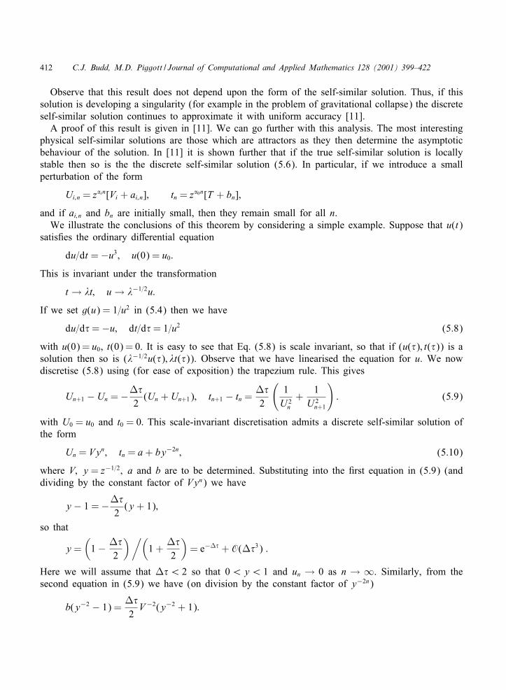
412 C.J. Budd, M.D. Piggott / Journal of Computational and Applied Mathematics 128 (2001) 399–422
Observe that this result does not depend upon the form of the self-similar solution. Thus, if thissolution is developing a singularity (for example in the problem of gravitational collapse) the discreteself-similar solution continues to approximate it with uniform accuracy [11].
A proof of this result is given in [11]. We can go further with this analysis. The most interestingphysical self-similar solutions are those which are attractors as they then determine the asymptoticbehaviour of the solution. In [11] it is shown further that if the true self-similar solution is locallystable then so is the the discrete self-similar solution (5.6). In particular, if we introduce a smallperturbation of the form
Ui;n = z�in[Vi + ai;n]; tn = z�0n[T + bn];
and if ai;n and bn are initially small, then they remain small for all n.We illustrate the conclusions of this theorem by considering a simple example. Suppose that u(t)
satis8es the ordinary di'erential equation
du=dt =−u3; u(0) = u0:
This is invariant under the transformation
t → �t; u→ �−1=2u:
If we set g(u) = 1=u2 in (5.4) then we have
du=d$ =−u; dt=d$ = 1=u2 (5.8)
with u(0) = u0, t(0) = 0. It is easy to see that Eq. (5.8) is scale invariant, so that if (u($); t($)) is asolution then so is (�−1=2u($); �t($)). Observe that we have linearised the equation for u. We nowdiscretise (5.8) using (for ease of exposition) the trapezium rule. This gives
Un+1 − Un =−S$2
(Un + Un+1); tn+1 − tn =S$2
(1U 2
n
+1
U 2n+1
): (5.9)
with U0 = u0 and t0 = 0: This scale-invariant discretisation admits a discrete self-similar solution ofthe form
Un = Vyn; tn = a + by−2n; (5.10)
where V; y = z−1=2; a and b are to be determined. Substituting into the 8rst equation in (5.9) (anddividing by the constant factor of Vyn) we have
y − 1 =−S$2
(y + 1);
so that
y =(
1− S$2
)/(1 +
S$2
)= e−S$ + O(S$3) :
Here we will assume that S$¡ 2 so that 0¡y¡ 1 and un → 0 as n → ∞. Similarly, from thesecond equation in (5.9) we have (on division by the constant factor of y−2n)
b(y−2 − 1) =S$2V−2(y−2 + 1):

C.J. Budd, M.D. Piggott / Journal of Computational and Applied Mathematics 128 (2001) 399–422 413
Hence, combining results gives
b =S$2V−2
(1 + y2
1− y2
); y =
1−S$=21 + S$=2
: (5.11)
Applying the initial conditions also gives V = u0 and a + b = 0: Thus
b =
[12
+S$2
8+ O(S$3)
]u−2
0 :
Hence, from the identity
tn = a + bz−2n = a + b(u0=Un)2;
we have
tn =
[12
+S$2
8+ O(S$3)
](U−2
n − u−20 ):
After some manipulation we then have
Un = u0
√1 + (S$2=4) + O(S$3)
2tnu20 + 1 + (S$2=4) + O(S$3)
: (5.12)
We now compare expression (5.12) with the exact solution which is given by
u(t) = u0
√1
2tu20 + 1
: (5.13)
This is, in fact, a self-similar solution with respect to the translated time s = t + u−20 =2: Expanding
the expression for Un and rearranging, then gives (for the case tn ¿ 0)
Un − u(tn) =1
16u0tnS$2 + O(S$3):
Observe that this error is (i) of the correct order for the trapezium rule and (ii) the error decays astn →∞.
6. Scale-invariant partial di erential equations
As it is diBcult to give a general theory for the convergence of numerical methods for scaleinvariant partial di'erential equations, we consider numerical methods as applied to the three exam-ples described in Section 2. To simplify our discussions, we consider the case of semi-discretisationsonly. These results can then easily be extended to full discretisations by using the theory outlinedin the previous section.
6.1. The porous medium equation
Some of these results can be found in the paper [7]. As described, the equation
ut = (uux)x = (u2=2)xx;

414 C.J. Budd, M.D. Piggott / Journal of Computational and Applied Mathematics 128 (2001) 399–422
has self-similar solutions of constant 8rst integral (2.6). Both these, and the solution from generalcompactly supported initial data, are compactly supported and have interfaces at points s− and s+
which move at a 8nite speed. To discretise this equation we introduce an adaptive mesh X (%; t)such that X (0; t) = s− and X (1; t) = s+. To determine X we use a monitor function and a movingmesh partial di'erential equation. As the evolution of the porous medium equation is fairly gentle itis possible to use the mesh equation (4.13) without fear of instability in the mesh. This then allowsa wide possible choice of scale-invariant monitor functions of the form M (u) = u�. A convenientfunction to use is
M (u) = u;
the choice of which is strongly motivated by the conservation law∫ s+
s−u dx = C:
Here C is a constant which we can take to equal 1 without loss of generality. Setting M = u andC = 1 in (4.13) gives∫ X
s−u dx = %; (6.1)
so that on di'erentiation with respect to % we have
uX% = 1; (6.2)
as the equation for the mesh which we will discretise. Note that this is invariant under the groupaction u→ �−1=3u; X → �1=3X . Now, di'erentiating (6.1) with respect to t gives
0 = Xtu +∫ X
s−ut dx = Xtu +
∫ X
s−(uux)x dx = u(Xt + ux):
Thus, for the continuous problem we also have that X satis8es the equation
Xt =−ux: (6.3)
Substituting (6.2) and (6.3) into the rescaled equation (4.5) gives, after some manipulation, thefollowing equation for u in the computational coordinates:
u(%; t)t = 12u
2(u2)%%: (6.4)
Eqs. (6.2)–(6.4) have a set of self-similar solutions of the form
u(%; t) = (t + C)−1=3w(%); X (%; t) = (t − C)1=3Y (%); (6.5)
where C is arbitrary and the functions w and Y satisfy di'erential equations in % only. Now, considersemi-discretisations of (6.2) and (6.4) so that we introduce discrete approximations Ui(t) and Xi(t)to the continuous functions u(%; t) and X (%; t) over the computational mesh
% = i=N; 16i6(N − 1)
with U0(t) =UN (t) = 0: A simple centred semi-discretisation of (6.4) for 16i6(N − 1) is given by
dUi
dt=
N 2
2U 2
i (U 2i+1 − 2U 2
i + U 2i−1): (6.6)

C.J. Budd, M.D. Piggott / Journal of Computational and Applied Mathematics 128 (2001) 399–422 415
To de8ne the mesh Xi we discretise (6.2) to give the algebraic system
(Xi+1 − Xi)(Ui+1 + Ui) = 2=N; 06i6(N − 1): (6.7)
We observe that this procedure has the geometric property of automatically conserving the discretemass
N−1∑i=0
(Xi+1 − Xi)(Ui+1 + Ui): (6.8)
An additional equation is needed to close the set of equations for the unknowns Xi and we do thisby insisting that (as in the true solution) the discrete centre of mass is conserved (without loss ofgenerality at 0), so that
N−1∑i=0
(X 2i+1 − X 2
i )(Ui+1 + Ui) = 0: (6.9)
Observe that Eq. (6.6) for the solution and Eqs. (6.7), (6.9) for the mesh have decoupled in thissystem. This makes it much easier to analyse. We discuss generalisations of this principle in aforthcoming paper [12]. In particular (6.6) has two key geometrical features. Firstly, it is invariantunder the group action
t → �t; Ui → �−1=3Ui:
Thus it admits a (semi) discrete self-similar solution of the form
U i(t) = (t + C)−1=3Wi; (6.10)
where Wi ¿ 0 satis8es an algebraic equation approximating the di'erential equation for w(%). Observethat for all C we have
t1=3U i → Wi:
Secondly, the discretisation satis8es a maximum principle, so that if Ui(t) and Vi(t) are two solutionswith Ui(0)¡Vi(0) for all i then Ui(t)¡Vi(t) for all i. (See [12]).
The consequences of these two results are profound. Suppose that Ui(0)¿ 0 is a general set ofinitial data. By choosing values of C appropriately (say C = t0 and C = t1) we can 8nd values suchthat
t−1=30 Wi ¡Ui(0)¡t−1=3
1 Wi; 16i6(N − 1):
Consequently, applying the maximum principle to the self-similar solution we then have thatfor all t
(t + t0)−1=3Wi ¡Ui(t)¡ (t + t1)−1=3Wi; 16i6(N − 1)
and hence we have the convergence result
t1=3Ui(t)→ Wi; (6.11)
showing that the solution Ui and hence the mesh Xi converges globally to the self-similar solution.Hence the numerical scheme is predicting precisely the correct asymptotic behaviour. This is becausethe discretisation has the same underlying geometry as the partial di'erential equation.

416 C.J. Budd, M.D. Piggott / Journal of Computational and Applied Mathematics 128 (2001) 399–422
Fig. 1. Convergence of the solution in the computational domain and invariance of the computed mesh.
We illustrate this result by performing a computation. Since the equations for the solution andthe equations for the mesh are decoupled, we may consider them separately. Firstly, the ODEs forthe solution u in the computational domain are integrated usind a third-order BDF method. We canthen simply solve for the mesh by inverting a linear system at each time level, assuming we havesymmetric initial data so that the centre of mass is at x = 0. Fig. 1 shows a solution with arbitraryinitial data being squeezed between two discrete self-similar solutions. The self-similar solutionsshown here are those with C taking the values 0:9 and 2:3.
6.2. The nonlinear Schr>odinger equation
We will summarise the method described in [5] for computing the radially symmetric blow-upsolutions of the nonlinear Schr3odinger equation (2.7) which become in8nite at the origin in a 8nitetime T . Previous computations [39] have used the method of dynamic rescaling which is closelyrelated to the scale-invariant methods, but lacks the generality of the approach we describe. Eq. (2.7)is invariant under the action of the two groups (2.8), (2.9), with an unknown coupling constant a.It is immediate from the phase invariance (2.9) that the required monitor function M (x; u; ux) mustbe of the form
M (x; u; ux) = M (x; |u|; |ux|):The mesh equation (4.14) applied to solutions which become in8nite in a 8nite time leads to unstablemeshes, and instead we use the stabilised equation (4.16). As a possible ansatz for a monitor functionleading to solutions invariant under the scaling (2.8) we may use
M (x; |u|; |ux|) = x�|u|�|ux|�
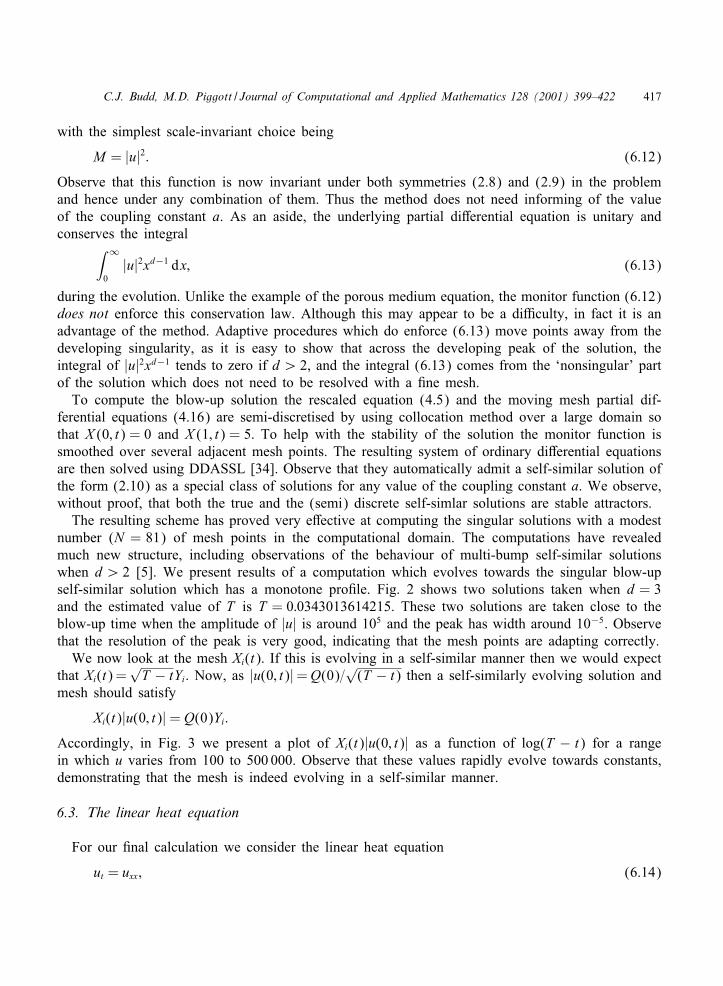
C.J. Budd, M.D. Piggott / Journal of Computational and Applied Mathematics 128 (2001) 399–422 417
with the simplest scale-invariant choice being
M = |u|2: (6.12)
Observe that this function is now invariant under both symmetries (2.8) and (2.9) in the problemand hence under any combination of them. Thus the method does not need informing of the valueof the coupling constant a. As an aside, the underlying partial di'erential equation is unitary andconserves the integral∫ ∞
0|u|2xd−1 dx; (6.13)
during the evolution. Unlike the example of the porous medium equation, the monitor function (6.12)does not enforce this conservation law. Although this may appear to be a diBculty, in fact it is anadvantage of the method. Adaptive procedures which do enforce (6.13) move points away from thedeveloping singularity, as it is easy to show that across the developing peak of the solution, theintegral of |u|2xd−1 tends to zero if d¿ 2, and the integral (6.13) comes from the ‘nonsingular’ partof the solution which does not need to be resolved with a 8ne mesh.
To compute the blow-up solution the rescaled equation (4.5) and the moving mesh partial dif-ferential equations (4.16) are semi-discretised by using collocation method over a large domain sothat X (0; t) = 0 and X (1; t) = 5: To help with the stability of the solution the monitor function issmoothed over several adjacent mesh points. The resulting system of ordinary di'erential equationsare then solved using DDASSL [34]. Observe that they automatically admit a self-similar solution ofthe form (2.10) as a special class of solutions for any value of the coupling constant a. We observe,without proof, that both the true and the (semi) discrete self-simlar solutions are stable attractors.
The resulting scheme has proved very e'ective at computing the singular solutions with a modestnumber (N = 81) of mesh points in the computational domain. The computations have revealedmuch new structure, including observations of the behaviour of multi-bump self-similar solutionswhen d¿ 2 [5]. We present results of a computation which evolves towards the singular blow-upself-similar solution which has a monotone pro8le. Fig. 2 shows two solutions taken when d = 3and the estimated value of T is T = 0:0343013614215. These two solutions are taken close to theblow-up time when the amplitude of |u| is around 105 and the peak has width around 10−5. Observethat the resolution of the peak is very good, indicating that the mesh points are adapting correctly.
We now look at the mesh Xi(t). If this is evolving in a self-similar manner then we would expectthat Xi(t) =
√T − tYi. Now, as |u(0; t)|=Q(0)=
√(T − t) then a self-similarly evolving solution and
mesh should satisfy
Xi(t)|u(0; t)|= Q(0)Yi:
Accordingly, in Fig. 3 we present a plot of Xi(t)|u(0; t)| as a function of log(T − t) for a rangein which u varies from 100 to 500 000. Observe that these values rapidly evolve towards constants,demonstrating that the mesh is indeed evolving in a self-similar manner.
6.3. The linear heat equation
For our 8nal calculation we consider the linear heat equation
ut = uxx; (6.14)
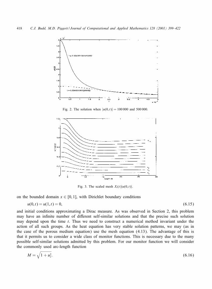
418 C.J. Budd, M.D. Piggott / Journal of Computational and Applied Mathematics 128 (2001) 399–422
Fig. 2. The solution when |u(0; t)| = 100 000 and 500 000.
Fig. 3. The scaled mesh Xi(t)|u(0; t)|.
on the bounded domain x ∈ [0; 1], with Dirichlet boundary conditions
u(0; t) = u(1; t) = 0; (6.15)
and initial conditions approximating a Dirac measure. As was observed in Section 2, this problemmay have an in8nite number of di'erent self-similar solutions and that the precise such solutionmay depend upon the time t. Thus we need to construct a numerical method invariant under theaction of all such groups. As the heat equation has very stable solution patterns, we may (as inthe case of the porous medium equation) use the mesh equation (4.13). The advantage of this isthat it permits us to consider a wide class of monitor functions. This is necessary due to the manypossible self-similar solutions admitted by this problem. For our monitor function we will considerthe commonly used arc-length function
M =√
1 + u2x : (6.16)

C.J. Budd, M.D. Piggott / Journal of Computational and Applied Mathematics 128 (2001) 399–422 419
As was observed earlier, this function is not scale invariant in general. However, if ux is large, thenM to a 8rst approximation is given by |ux| which is scale invariant. We can regard arc-length as aregularisation of this function. When |ux| is small then arc-length reduces to 1 which is (trivially)scale invariant and leads to a uniform mesh. This is appropriate during the 8nal evolution of thesolution. This monitor function also has the advantage that it is not too much a'ected by the boundaryconditions. Thus the mesh X (%; t) must satisfy∫ X
0
√1 + u2
x dx = %∫ 1
0
√1 + u2
x dx: (6.17)
If |ux| is large and u has a single maximum then
%∫ 1
0
√1 + u2
x dx ≈ 2%max(u): (6.18)
We now consider how the resulting continuous mesh behaves for solutions in the two asymptoticregimes described by (2.16) and (2.17). Consider 8rst (2.16), in which we will assume that t issuBciently small so that this self-similar description is appropriate. In this case we have∫ X
0
A√te−(x−x0)2=4t dx = %
∫ 1
0
A√te−(x−x0)2=4t dx
with u having a single maximum of A=√t � 1 at x = x0. Now, as t is small, |ux| is large, apart
from the immediate neighbourhood of the point x0 and∫ X
0
√1 + u2
x dx ≈∫ X
0|ux| dx ≈ u(X ) if X ¡x0 or 2 max(u)− u(x) if X ¿x0:
It follows from (6.18) that if we are close to the peak of the solution then
A√te(X−x0)2=4t =
2A√t% if X ¡x0
and similarly
A√te(X−x0)2=4t =
2A√t(1− %) if X ¿x0:
The scaling invariance of the function |ux| has led to the same factor of A=√t arising in both sides
of this equation and allows us to simplify and solve it. The resulting mesh is then given by
X (%; t) ≈ x0 − 2√t√
log(1=2%); %¡ 12 ; (6.19)
X (%; t) ≈ x0 + 2√t√
log(1=2(1− %)); %¿ 12 : (6.20)
(We have ignored here the behaviour very close to x0 where ux vanishes and M is very locallyapproximated by 1.)
Observe that this mesh automatically clusters points around the maximum at x=x0 of the solutionof the heat equation and that these points evolve in a correct self-similar manner consistent with theunderlying scaling. Indeed, X (%; t) evolves as
X (%; t) ≈ x0 +√tY (%)
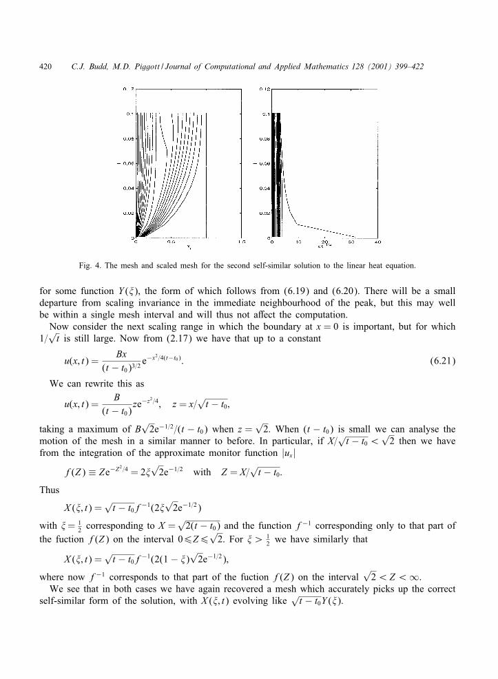
420 C.J. Budd, M.D. Piggott / Journal of Computational and Applied Mathematics 128 (2001) 399–422
Fig. 4. The mesh and scaled mesh for the second self-similar solution to the linear heat equation.
for some function Y (%), the form of which follows from (6.19) and (6.20). There will be a smalldeparture from scaling invariance in the immediate neighbourhood of the peak, but this may wellbe within a single mesh interval and will thus not a'ect the computation.
Now consider the next scaling range in which the boundary at x = 0 is important, but for which1=√t is still large. Now from (2.17) we have that up to a constant
u(x; t) =Bx
(t − t0)3=2e−x2=4(t−t0): (6.21)
We can rewrite this as
u(x; t) =B
(t − t0)ze−z2=4; z = x=
√t − t0;
taking a maximum of B√
2e−1=2=(t − t0) when z =√
2. When (t − t0) is small we can analyse themotion of the mesh in a similar manner to before. In particular, if X=
√t − t0 ¡
√2 then we have
from the integration of the approximate monitor function |ux|f(Z) ≡ Ze−Z2=4 = 2%
√2e−1=2 with Z = X=
√t − t0:
Thus
X (%; t) =√t − t0f−1(2%
√2e−1=2)
with %= 12 corresponding to X =
√2(t − t0) and the function f−1 corresponding only to that part of
the fuction f(Z) on the interval 06Z6√
2. For %¿ 12 we have similarly that
X (%; t) =√t − t0f−1(2(1− %)
√2e−1=2);
where now f−1 corresponds to that part of the fuction f(Z) on the interval√
2¡Z ¡∞.We see that in both cases we have again recovered a mesh which accurately picks up the correct
self-similar form of the solution, with X (%; t) evolving like√t − t0Y (%).
C.J. Budd, M.D. Piggott / Journal of Computational and Applied Mathematics 128 (2001) 399–422 421
Thus the use of the monitor-function-based approach for this example has allowed the mesh toevolve in the correct self-similar manner in the two cases, even though the self-similar solution istaking two rather di'erent forms. This example demonstrates the Dexibility of our approach.
We present, in Fig. 4, some calculations of the evolution of the mesh obtained by solving (6.17)in the regime for which we take u to be the self-similar solution (6.21). We see the mesh is initiallyscaling as
√tY (%) close to x = 0 and eventualy becomes uniform as ux → 0 everywhere.
7. Conclusions
We have shown in this review that scale-invariant di'erential equations are common in manyapplication areas and have interesting types of behaviour, with the form of the scaling underlying thesolutions of the equations not always apparent at 8rst inspection. Scale-invariant adaptive numericalmethods have the virtue of preserving many of the properties of such equations which are derivedfrom their scaling, including their asymptotic behaviour. These methods do not, however, compromisethe generality required of a numerical computational technique. The next stage of the work on theseideas is to develop them for problems which have scaling invariance in several spatial dimensions.This is the subject of our future work.
References
[1] A. Arakawa, Computational design for long-term numerical integration of the equations of Duid motion:two-dimensional incompressible Dow, J. Comput. Phys. 1 (1966) 119–143.
[2] G.I. Barenblatt, Scaling, self-similarity and intermediate asymptotics, Cambridge Univeristy Press, Cambridge, 1996.[3] J. Bebernes, D. Eberly, Mathematical Problems from Combustion Theory, Applied Mathematical Sciences, Vol. 83,
Springer, Berlin, 1989.[4] P.W. Bridgman, Dimensional Analysis, Yale University Press, New York, 1931.[5] C.J. Budd, S. Chen, R.D. Russell, New self-similar solutions of the nonlinear Schr3odinger equation with moving
mesh computations, J. Comput. Phys. 152 (1999) 756–789.[6] C.J. Budd, G.J. Collins, Symmetry based numerical methods for partial di'erential equations, in: D. GriBths,
D. Higham, G. Watson (Eds.), Numerical Analysis 1997, Pitman Research Notes in Mathematics Series, Vol. 380,Longman, New York, 1998, pp. 16–36.
[7] C.J. Budd, G.J. Collins, W.-Z. Huang, R.D. Russell, Self-similar discrete solutions of the porous medium equation,Philos. Trans. Roy. Soc. London A 357 (1999) 1047–1078.
[8] C.J. Budd, W.-Z. Huang, R.D. Russell, Moving mesh methods for problems with blow-up, SIAM J. Sci. Computut.17 (1996) 305–327.
[9] C.J. Budd, G.W. Hunt, M.A. Peletier, Self-similar fold evolution under prescribed end-shortening, J. Math. Geol. 31(1999) 989–1005.
[10] C.J. Budd, A. Iserles (Eds.), Geometric integration: numerical solution of di'erential equations on manifolds, Philos.Trans. Roy. Soc. London A 357 (1999) 943–1133.
[11] C.J. Budd, B. Leimkuhler, M.D. Piggott, Scaling invariance and adaptivity, in: Iserles, Norsett (Eds.), GeometricIntegration, 2000.
[12] C.J. Budd, M.D. Piggott, Symmetry invariance and the discrete maximum principle, in preparation.[13] I. Budiansky, G. Carrier, The pointless wedge, SIAM J. Appl. Math. 25 (1973) 378–387.[14] M.J.P. Cullen, J. Norbury, R.J. Purser, Generalised lagrangian solutions for atmospheric and oceanic Dows, SIAM
J. Appl. Math. 51 (1991) 20–31.[15] V.A. Dorodnitsyn, Finite di'erence methods entirely inheriting the symmetry of the original equations, in: N.
Ibragimov (Ed.), Modern Group Analysis: Advanced Analytical and Computational Methods in Mathematical Physics,1993, pp. 191–201.
422 C.J. Budd, M.D. Piggott / Journal of Computational and Applied Mathematics 128 (2001) 399–422
[16] V.A. Dorodnitsyn, Symmetry of 8nite-di'erence equations, in: N. Ibragimov (Ed.), CRC Handbook of Lie GroupAnalysis of Di'erential Equations, Vol. I: Symmetries, Exact Solutions and Conservation Laws, CRC Press, BocaRaton, FL, 1993, pp. 365–403.
[17] E.A. Dor8, L. O’C. Drury, Simple adaptive grids for 1-D initial value problems, J. Comput. Phys. 69 (1987)175–195.
[18] L. Dresner, Similarity solutions of nonlinear partial di'erential equations, Pitman Research Notes in Mathematics,Vol. 88, Longman, New York, 1983.
[19] K. Falconer, Fractal Geometry, Wiley, New York, 1990.[20] N. Goldenfeld, O. Martin, Y. Oono, Intermediate asymptotics and renormalization group theory, J. Sci. Comput. 4
(1989) 355–372.[21] M. Golubitsky, D. Schae'er, I. Stewart, Singularities and Groups in Bifurcation Theory, Applied Mathematica
Sciences, Vol. 69, Springer, Berlin, 1987.[22] J. Hulshof, J.L. Vazquez, Self-similar solutions of the second kind for the modi8ed porous medium equation, Eur.
J. Appl. Math. 5 (1994) 391–403.[23] W. Huang, Y. Ren, R.D. Russell, Moving mesh methods based on moving mesh partial di'erential equations, J.
Comput. Phys. 112 (1994) 279–290.[24] W. Huang, R.D. Russell, A high dimensional moving mesh strategy, Appl. Numer. Math. 26 (1999) 998–1015.[25] A. Iserles, Numerical methods on (and o' ) manifolds, in: F. Cucker, M. Shub (Eds.), Foundations of Computational
Mathematics, Springer, New York, 1997, pp. 180–189.[26] S. Kamenomostskaya, The asymptotic behaviour of the solution of the 8ltration equation, Israel J. Math. 14 (1973)
279–290.[27] A.N. Kolmogorov, The local structure of turbulence in incompressible Duids at very high Reynolds numbers, Dokl.
USSR Acad. Sci. 30 (4) (1941) 299–303.[28] B. Leimkuhler, Reversible adaptive regularisation: perturbed Kepler motion and classical atomic trajectories, Philos.
Trans. Roy. Soc. 357 (1999) 1101–1133.[29] E. Mans8eld, The di'erential algebra package diffgrob2, MapleTech 3 (1996) 33–37.[30] R. McLachlan, Symplectic integration of Hamiltonian wave equations, Numer. Math. 66 (1994) 465–492.[31] J.D. Murray, Mathematical biology, Springer, Berlin, 1989.[32] P. Olver, Applications of Lie Groups to Di'erential Equations, Springer, New York, 1986.[33] V. Pereyra, E.G. Sewell, Mesh selection for discrete solution of boundary problems in ordinary di'erential equations,
Numer. Math. 23 (1975) 261–268.[34] L. Petzold, A description of DDASSL, a di'erential=algebraic system solver, Report SAND82-8637, Sandia National
Laboratories, 1982.[35] M.H. Protter, H.F. Weinberger, Maximum Principles in Di'erential Equations, Springer, New York, 1984.[36] S. Reich, Backward error analysis for numerical integrators, SIAM J. Numer. Anal. 36 (1999) 1549–1570.[37] S. Reich, Finite volume methods for multi-symplectic PDEs, BIT 40 (2000) 559–582.[38] A. Samarskii, V. Galaktionov, S. Kurdyumov, A. Mikhailov, Blow-up in Quasilinear Parabolic Equations, de Gruyter,
Berlin, 1995.[39] C. Sulem, P.-L. Sulem, The Nonlinear Schr3odinger Equation, Applied Mathematical Sciences, Vol. 139, Springer,
Berlin, 1999.[40] J.L. Vazquez, An introduction to the mathematical theory of the porous medium equation, in: M. Delfour (Ed.),
Shape Optimisation and Free Boundaries, Kluwer Academic Publishers, Dordrecht, 1992, pp. 347–389.[41] V.E. Zakharov, E.A. Kuznetsov, Hamiltonian formalism for systems of hydrodynamic type, Soviet Sci. Rev. Section
C: Math. Phys. Rev 4 (1984) 167–220.[42] Ya. B. Zeldovich, Yu. P. Razier, Physics of Shock Waves and High Temperature Hydrodynamic Phenomena,
Academic Press, New York, 1967.

Journal of Computational and Applied Mathematics 128 (2001) 423–445www.elsevier.nl/locate/cam
A summary of numerical methods for time-dependentadvection-dominated partial di%erential equations
Richard E. Ewinga ; ∗, Hong Wangb
aInstitute for Scienti c Computation, Texas A&M University, College Station, Texas 77843-3404, USAbDepartment of Mathematics, University of South Carolina, Columbia, South Carolina 29208, USA
Received 30 September 1999; received in revised form 8 February 2000
Abstract
We give a brief summary of numerical methods for time-dependent advection-dominated partial di%erential equations(PDEs), including 4rst-order hyperbolic PDEs and nonstationary advection–di%usion PDEs. Mathematical models arisingin porous medium 5uid 5ow are presented to motivate these equations. It is understood that these PDEs also arise inmany other important 4elds and that the numerical methods reviewed apply to general advection-dominated PDEs. Weconduct a brief historical review of classical numerical methods, and a survey of the recent developments on the Eulerianand characteristic methods for time-dependent advection-dominated PDEs. The survey is not comprehensive due to thelimitation of its length, and a large portion of the paper covers characteristic or Eulerian–Lagrangian methods. c© 2001Elsevier Science B.V. All rights reserved.
MSC: 65M; 65N; 76M; 76R
Keywords: Advection–di%usion equations; Characteristic methods; Eulerian methods; Numerical simulations
1. Mathematical models
We present mathematical models arising in subsurface porous medium 5uid 5ow (e.g. subsurfacecontaminant transport, reservoir simulation) to motivate time-dependent advection-dominated PDEs.These types of PDEs also arise in many other important 4elds, such as the mathematical modeling ofaerodynamics, 5uid dynamics (e.g. Euler equations, Navier–Stokes equations) [70,93], meteorology[90], and semiconductor devices [72].
∗ Corresponding author.E-mail address: [email protected] (R.E. Ewing).
0377-0427/01/$ - see front matter c© 2001 Elsevier Science B.V. All rights reserved.PII: S 0377-0427(00)00522-7

424 R.E. Ewing, H. Wang / Journal of Computational and Applied Mathematics 128 (2001) 423–445
1.1. Miscible 8ows
A mathematical model used for describing fully saturated 5uid 5ow processes through porousmedia is derived by using the mass balance equation for the 5uid mixture [5,40]
@@t
(��)−� ·(�K�
(�p− �g))
= q; x ∈ ; t ∈ [0; T ]: (1.1)
Here is the physical domain, u, p, and � are the Darcy velocity, the pressure, and the massdensity of the 5uid, K (x) is the absolute permeability of the medium, � is the dynamic viscosityof the 5uid, g is the acceleration vector due to gravity, and q represents the source and sink terms,which is often modeled via point or line sources and sinks.
The transport of a speci4c component in the 5uid mixture is governed by the mass conservationfor the component and is expressed as
@(�c)@t
+� · (uc)−� · (D(u)�c) = Gcq; x ∈ ; t ∈ [0; T ]: (1.2)
Here c, a fraction between 0 and 1, represents the concentration of the component, � is the porosityof the medium, Gc(x; t) is either the speci4ed concentrations of the injected 5uids at sources or theresident concentrations at sinks, and D(u) is the di%usion–dispersion tensor.
1.2. Multiphase 8ows
When either air or a nonaqueous-phase liquid (NAPL) contaminant is present in groundwatertransport processes, this phase is immiscible with the water phase and the two phases 5ow simulta-neously in the 5ow process. Likewise, in the immiscible displacement in petroleum production, theoil phase and the water phase are immiscible. In both cases, there is no mass transfer between thetwo phases and so the following equations hold for each phase [5,17,19,40]:
@@t
(��jSj)−� ·(�jKkrj
�j�pj
)= �jqj; x ∈ ; t ∈ [0; T ]: (1.3)
Here Sj, uj, �j, pj, krj, �j, and qj are the saturation, velocity, density, pressure, relative permeability,viscosity, and source and sink terms for the phase j. The indices j=n and w stand for the nonwettingand wetting phases, respectively. The saturations Sn and Sw satisfy the relation Sn + Sw = 1.
Eqs. (1.3) may be rearranged in a form that resembles Eqs. (1.1) and (1.2) by letting Sn = 1−Sw.The pressure between the two phases is described by the capillary pressure pc(Sw) = pn − pw. Theglobal pressure p and total velocity u of a two-phase 5ow model is given by the following equations[21]:
SnCnDpDt−� · (K��p) = q(x; Sw; p); x ∈ ; t ∈ [0; T ]; (1.4)
where (D=Dt) = �(@=@t) + (un=Sn) · � and p = 12 (pn + pw) + 1
2
∫ SSc
((�n − �w)=�)(dpc=d�) d� withpc(Sc) = 0. The total mobility � = �n + �w, the phase mobility �j = krj=�j, and the compressibilityCj = (1=�j)(d�j=dpj) are functions of time and space.
R.E. Ewing, H. Wang / Journal of Computational and Applied Mathematics 128 (2001) 423–445 425
The governing equation for the wetting phase now has a form
�@Sw
@t+� · (f(Sw)u −D(Sw)�Sw) = qw; x ∈ ; t ∈ [0; T ]; (1.5)
where �c = �n − �w. The capillary di%usion D(Sw) = −K�nfw(dpc=dSw) and the fractional 5owfunctions fj = �j=�.
In practice, the di%usion term in Eq. (1.2) or (1.5) is often a small phenomenon relative toadvection. Hence, these equations are time-dependent advection–di%usion partial di%erential equations(PDEs) in terms of the concentration c or the saturation S. In particular, Eq. (1.5) has an S-shapednonlinear 5ux function f and a degenerate capillary di%usion term [19,40]. Sometimes the di%usionphenomenon is so small that its e%ect is neglected. In this case, Eq. (1.2) or (1.5) is reduced toa 4rst-order hyperbolic PDE. Finally, initial and boundary conditions also need to be speci4ed toclose the system (1.1)–(1.2) or (1.4)–(1.5).
2. Conventional �nite di�erence and �nite element methods
We carry out a brief historical review of classical numerical methods in this section and a surveyof the recent developments on the Eulerian and characteristic methods in the next section primarilyfor time-dependent advection-dominated PDEs, including 4rst-order hyperbolic PDEs and nonsta-tionary advection–di%usion PDEs. Because of the extensive research carried out in these areas, itis impossible to describe adequately all these developments in the space available. Hence, this re-view is not comprehensive in that we try to describe and review only some representatives of thehuge amount of works in the literature. Notice that since relatively more references and surveypapers can be found on the Eulerian methods for unsteady state advection-dominated PDEs, weintend to use a relatively large portion to cover characteristic or Eulerian–Lagrangian methods foradvection-dominated PDEs. Finally, we refer interested readers to the works of Morton [73] andRoos et al. [86] for detailed descriptions on the recent developments for the numerical methods forstationary advection–di%usion PDEs.
It is well known that advection-dominated PDEs present serious numerical diIculties due to themoving steep fronts present in the solutions of advection–di%usion transport PDEs or shock discon-tinuities in the solutions of pure advection PDEs or advection–di%usion PDEs with degenerate dif-fusion. Additional diIculties include the strong couplings and nonlinearities of advection-dominatedPDE systems, the e%ect of the singularities at point=line sources and sinks, the strong heterogene-ity of the coeIcients, anisotropic di%usion–dispersion in tensor form, and the enormous sizes of4eld-scale applications.
2.1. Finite di:erence methods (FDMs)
Due to their simplicity, FDMs were 4rst used in solving advection-dominated PDEs. For conve-nience, of presentation, we consider the one-dimensional constant-coeIcient analogue of Eq. (1.2)
@c@t
+ V@c@x− D
@2c@x2
= 0; x ∈ (a; b); t ∈ [0; T ] (2.1)

426 R.E. Ewing, H. Wang / Journal of Computational and Applied Mathematics 128 (2001) 423–445
and assume a uniform spatial and temporal partition xi =a+ iKx for i=0; 1; : : : ; I with Kx=(b−a)=Iand tm = mKt for m = 0; 1; : : : ; M with Kt = T=M .
We de4ne the Courant number Cr = VKt=Kx and the Peclet number Pe = VKx=D. It is knownthat the solution to the space-centered explicit scheme
cm+1i − cmi
Kt+ V
cmi+1 − cmi−1
2Kx− D
cmi+1 − 2cmi + cmi−1
(Kx)2= 0 (2.2)
does not oscillate only when the Peclet number Pe62 and the CFL condition (Cr61) is satis4ed[30,81]. For Pe¿ 2, damped oscillations occur with nonreal eigenvalues [48,81]. Furthermore, forthe linear hyperbolic PDE
@c@t
+ V@c@x
= 0; x ∈ (a; b); t ∈ [0; T ]; (2.3)
which can be viewed as a limiting case of D→ 0 in Eq. (2.1), the corresponding scheme to scheme(2.2)
cm+1i − cmi
Kt+ V
cmi+1 − cmi−1
2Kx= 0 (2.4)
is unconditionally unstable [48,94].The upwind FDM (UFDM) uses a one-sided 4nite di%erence in the upstream direction to approx-
imate the advection term in the transport PDE (2.1) and can be expressed as follows (assumingV¿0):
cm+1i − cmi
Kt+ V
cmi − cmi−1
2Kx− D
cmi+1 − 2cmi + cmi−1
(Kx)2= 0: (2.5)
The Lax–Friedrichs schemecm+1i − (cmi+1 + cmi−1)=2
Kt+ V
cmi+1 − cmi−1
2Kx− D
cmi+1 − 2cmi + cmi−1
(Kx)2= 0 (2.6)
is obtained by replacing cmi in the 4rst term in Eq. (2.2) by its mean value (cmi+1 + cmi−1)=2.
Remark 1. Schemes (2.5) and (2.6) eliminate the nonphysical oscillations present in Scheme (2.2),and generate stable solutions even for very complicated multiphase and multicomponent 5ows. Itcan be shown that the UFDM scheme is actually a second-order approximation to Eq. (2.1) witha modi4ed di%usion D(1 + (Pe=2)(1 − Cr)), while the Lax–Friedrichs scheme is a second-orderapproximation to Eq. (2.1) with an extra numerical di%usion ((Kx)2=2Kt)(1−Cr2) [40,59,70]. Hence,these methods introduce excessive numerical di%usion and the numerical solutions are dependent upongrid orientation. Detailed description on the theory and the use of modi4ed equations can be foundin [59,70,110].
The Lax–Wendro% scheme is based on the Taylor series expansion and Eq. (2.3)
c(x; tm+1) = c(x; tm) + Kt@c(x; tm)
@t+
(Kt)2
2@2c(x; tm)
@t2+ O((Kt)3)
= c(x; tm)− VKt@c(x; tm)
@x+
(VKt)2
2@2c(x; tm)
@x2+ O((Kt)3): (2.7)

R.E. Ewing, H. Wang / Journal of Computational and Applied Mathematics 128 (2001) 423–445 427
Dropping the O((Kt)3) term in Eq. (2.7) and using centered di%erences to approximate the spatialderivatives yields the Lax–Wendro% scheme
cm+1i = cmi −
Cr2
(cmi+1 − cmi−1) +Cr2
2(cmi+1 − 2cmi + cmi−1); (2.8)
which is a second-order scheme.The Beam–Warming scheme is a one-sided version of the Lax–Wendro% scheme. It uses second-
order accurate one-sided di%erences to approximate the spatial derivatives in Eq. (2.7)
cm+1i = cmi −
Cr2
(3cmi − 4cmi−1 + cmi−2) +Cr2
2(cmi − 2cmi−1 + cmi−2): (2.9)
Remark 2. The Lax–Wendro% scheme and the Beam–Warming scheme give third-order approxima-tions to the modi4ed advection–dispersion equation
@c@t
+ V@c@x− �
@3c@x3
= 0; x ∈ (a; b); t ∈ [0; T ]
with � = (V (Kx)2=6)(Cr2 − 1) for (2.8) and (V (Kx)2=6)(2 − 3Cr + Cr2) for (2.9). The theory ofdispersive waves and its utility in the study of numerical methods are covered in [97,112], whichshow that the Lax–Wendro% scheme tends to develop oscillations behind shock fronts while theBeam–Warming scheme tends to develop oscillations in front of shock fronts.
Remark 3. Solving Eq. (2.3) yields c(x; tm+1)=c(x−VKt; tm). When the CFL condition is satis4ed,the UPFD or the Lax–Friedrichs scheme can be viewed as an linear interpolation of c(x− VKt; tm)by the nodal values c(xi−1; tm) and c(xi; tm), or c(xi−1; tm) and c(xi+1; tm), respectively. This explainswhy these schemes are free of oscillations and introduce smearing from another point of view [70].Second, because UFDM takes advantage of upstream information, it is slightly more accurate than theLax–Friedrichs scheme. On the other hand, the latter is symmetric and can be easily implemented,which is an important feature for nonlinear hyperbolic conservation laws. In contrast, the Lax–Wendro% scheme (2.8) or Beam–Warming scheme (2.9) can be viewed as a quadratic interpolationof c(x−VKt; tm) by the nodal values c(xi−1; tm), c(xi; tm), and c(xi+1; tm), or c(xi; tm), c(xi+1; tm), andc(xi+2; tm). This is why they introduce oscillations across shock discontinuities.
The leap-frog scheme for Eq. (2.3) is obtained by replacing the forward di%erence in time in(2.4) by a centered di%erence
cm+1i − cm−1
i
Kt+ V
cmi+1 − cmi−1
2Kx= 0: (2.10)
Scheme (2.10) has an improved truncation error of O((Kx)2 +(Kt)2), but it is a multi-level scheme.This leads to increased computational storage, a particular disadvantage for large multi-dimensionalnonlinear systems.
These methods can be extended to solve nonlinear hyperbolic conservation laws
@c@t
+@f(c)@x
= 0; x ∈ (a; b); t ∈ [0; T ] (2.11)
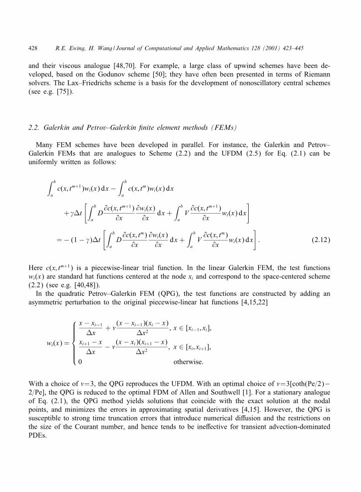
428 R.E. Ewing, H. Wang / Journal of Computational and Applied Mathematics 128 (2001) 423–445
and their viscous analogue [48,70]. For example, a large class of upwind schemes have been de-veloped, based on the Godunov scheme [50]; they have often been presented in terms of Riemannsolvers. The Lax–Friedrichs scheme is a basis for the development of nonoscillatory central schemes(see e.g. [75]).
2.2. Galerkin and Petrov–Galerkin nite element methods (FEMs)
Many FEM schemes have been developed in parallel. For instance, the Galerkin and Petrov–Galerkin FEMs that are analogues to Scheme (2.2) and the UFDM (2.5) for Eq. (2.1) can beuniformly written as follows:
∫ b
ac(x; tm+1)wi(x) dx −
∫ b
ac(x; tm)wi(x) dx
+ !Kt
[∫ b
aD@c(x; tm+1)
@x@wi(x)@x
dx +∫ b
aV@c(x; tm+1)
@xwi(x) dx
]
=− (1− !)Kt
[∫ b
aD@c(x; tm)
@x@wi(x)@x
dx +∫ b
aV@c(x; tm)
@xwi(x) dx
]: (2.12)
Here c(x; tm+1) is a piecewise-linear trial function. In the linear Galerkin FEM, the test functionswi(x) are standard hat functions centered at the node xi and correspond to the space-centered scheme(2.2) (see e.g. [40,48]).
In the quadratic Petrov–Galerkin FEM (QPG), the test functions are constructed by adding anasymmetric perturbation to the original piecewise-linear hat functions [4,15,22]
wi(x) =
x − xi−1
Kx+ "
(x − xi−1)(xi − x)Kx2
; x ∈ [xi−1; xi];
xi+1 − xKx
− "(x − xi)(xi+1 − x)
Kx2; x ∈ [xi; xi+1];
0 otherwise:
With a choice of "=3, the QPG reproduces the UFDM. With an optimal choice of "=3[coth(Pe=2)−2=Pe], the QPG is reduced to the optimal FDM of Allen and Southwell [1]. For a stationary analogueof Eq. (2.1), the QPG method yields solutions that coincide with the exact solution at the nodalpoints, and minimizes the errors in approximating spatial derivatives [4,15]. However, the QPG issusceptible to strong time truncation errors that introduce numerical di%usion and the restrictions onthe size of the Courant number, and hence tends to be ine%ective for transient advection-dominatedPDEs.
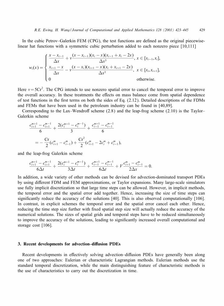
R.E. Ewing, H. Wang / Journal of Computational and Applied Mathematics 128 (2001) 423–445 429
In the cubic Petrov–Galerkin FEM (CPG), the test functions are de4ned as the original piecewise-linear hat functions with a symmetric cubic perturbation added to each nonzero piece [10,111]
wi(x) =
x − xi−1
Kx+ "
(x − xi−1)(xi − x)(xi−1 + xi − 2x)Kx3
; x ∈ [xi−1; xi];
xi+1 − xKx
− "(x − xi)(xi+1 − x)(xi + xi+1 − 2x)
Kx3; x ∈ [xi; xi+1];
0 otherwise:
Here "= 5Cr2. The CPG intends to use nonzero spatial error to cancel the temporal error to improvethe overall accuracy. In these treatments the e%ects on mass balance come from spatial dependenceof test functions in the 4rst terms on both the sides of Eq. (2.12). Detailed descriptions of the FDMsand FEMs that have been used in the petroleum industry can be found in [40,89].
Corresponding to the Lax–Wendro% scheme (2.8) and the leap-frog scheme (2.10) is the Taylor–Galerkin scheme
cm+1i+1 − cm−1
i+1
6+
2(cm+1i − cm−1
i )3
+cm+1i−1 − cm−1
i−1
6
=− Cr2
(cmi+1 − cmi−1) +Cr2
2(cmi+1 − 2cmi + cmi−1);
and the leap-frog Galerkin scheme
cm+1i+1 − cm−1
i+1
6Kt+
2(cm+1i − cm−1
i )3Kt
+cm+1i−1 − cm−1
i−1
6Kt+ V
cmi+1 − cmi−1
2Kx= 0:
In addition, a wide variety of other methods can be devised for advection-dominated transport PDEsby using di%erent FDM and FEM approximations, or Taylor expansions. Many large-scale simulatorsuse fully implicit discretization so that large time steps can be allowed. However, in implicit methods,the temporal error and the spatial error add together. Hence, increasing the size of time steps cansigni4cantly reduce the accuracy of the solutions [40]. This is also observed computationally [106].In contrast, in explicit schemes the temporal error and the spatial error cancel each other. Hence,reducing the time step size further with 4xed spatial step size will actually reduce the accuracy of thenumerical solutions. The sizes of spatial grids and temporal steps have to be reduced simultaneouslyto improve the accuracy of the solutions, leading to signi4cantly increased overall computational andstorage cost [106].
3. Recent developments for advection–di�usion PDEs
Recent developments in e%ectively solving advection–di%usion PDEs have generally been alongone of two approaches: Eulerian or characteristic Lagrangian methods. Eulerian methods use thestandard temporal discretization, while the main distinguishing feature of characteristic methods isthe use of characteristics to carry out the discretization in time.
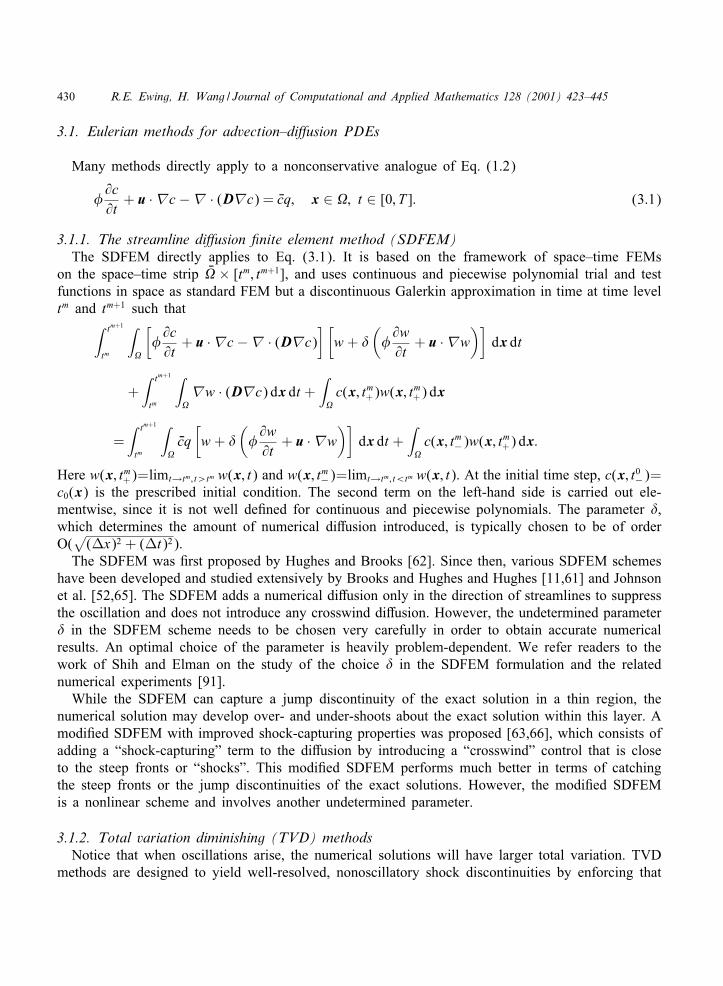
430 R.E. Ewing, H. Wang / Journal of Computational and Applied Mathematics 128 (2001) 423–445
3.1. Eulerian methods for advection–di:usion PDEs
Many methods directly apply to a nonconservative analogue of Eq. (1.2)
�@c@t
+ u ·�c −� · (D�c) = Gcq; x ∈ ; t ∈ [0; T ]: (3.1)
3.1.1. The streamline di:usion nite element method (SDFEM)The SDFEM directly applies to Eq. (3.1). It is based on the framework of space–time FEMs
on the space–time strip G × [tm; tm+1], and uses continuous and piecewise polynomial trial and testfunctions in space as standard FEM but a discontinuous Galerkin approximation in time at time leveltm and tm+1 such that∫ tm+1
tm
∫
[�@c@t
+ u ·�c −� · (D�c)] [
w + #(�@w@t
+ u ·�w)]
dx dt
+∫ tm+1
tm
∫�w · (D�c) dx dt +
∫c(x; tm+)w(x; tm+) dx
=∫ tm+1
tm
∫
Gcq[w + #
(�@w@t
+ u ·�w)]
dx dt +∫c(x; tm−)w(x; tm+) dx:
Here w(x; tm+)=limt→tm; t¿tm w(x; t) and w(x; tm−)=limt→tm; t¡tm w(x; t). At the initial time step, c(x; t0−)=
c0(x) is the prescribed initial condition. The second term on the left-hand side is carried out ele-mentwise, since it is not well de4ned for continuous and piecewise polynomials. The parameter #,which determines the amount of numerical di%usion introduced, is typically chosen to be of orderO(√
(Kx)2 + (Kt)2).The SDFEM was 4rst proposed by Hughes and Brooks [62]. Since then, various SDFEM schemes
have been developed and studied extensively by Brooks and Hughes and Hughes [11,61] and Johnsonet al. [52,65]. The SDFEM adds a numerical di%usion only in the direction of streamlines to suppressthe oscillation and does not introduce any crosswind di%usion. However, the undetermined parameter# in the SDFEM scheme needs to be chosen very carefully in order to obtain accurate numericalresults. An optimal choice of the parameter is heavily problem-dependent. We refer readers to thework of Shih and Elman on the study of the choice # in the SDFEM formulation and the relatednumerical experiments [91].
While the SDFEM can capture a jump discontinuity of the exact solution in a thin region, thenumerical solution may develop over- and under-shoots about the exact solution within this layer. Amodi4ed SDFEM with improved shock-capturing properties was proposed [63,66], which consists ofadding a “shock-capturing” term to the di%usion by introducing a “crosswind” control that is closeto the steep fronts or “shocks”. This modi4ed SDFEM performs much better in terms of catchingthe steep fronts or the jump discontinuities of the exact solutions. However, the modi4ed SDFEMis a nonlinear scheme and involves another undetermined parameter.
3.1.2. Total variation diminishing (TVD) methodsNotice that when oscillations arise, the numerical solutions will have larger total variation. TVD
methods are designed to yield well-resolved, nonoscillatory shock discontinuities by enforcing that
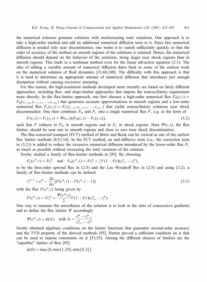
R.E. Ewing, H. Wang / Journal of Computational and Applied Mathematics 128 (2001) 423–445 431
the numerical schemes generate solutions with nonincreasing total variations. One approach is totake a high-order method and add an additional numerical di%usion term to it. Since this numericaldi%usion is needed only near discontinuities, one wants it to vanish suIciently quickly so that theorder of accuracy of the method on smooth regions of the solutions is retained. Hence, the numericaldi%usion should depend on the behavior of the solutions, being larger near shock regions than insmooth regions. This leads to a nonlinear method even for the linear advection equation (2.3). Theidea of adding a variable amount of numerical di%usion dates back to some of the earliest workon the numerical solution of 5uid dynamics [31,68,100]. The diIculty with this approach is thatit is hard to determine an appropriate amount of numerical di%usion that introduces just enoughdissipation without causing excessive smearing.
For this reason, the high-resolution methods developed more recently are based on fairly di%erentapproaches, including 5ux- and slope-limiter approaches that impose the nonoscillatory requirementmore directly. In the 5ux-limiter approach, one 4rst chooses a high-order numerical 5ux FH(c; i) =FH(ci−lH ; ci−l+1; : : : ; ci+rH ) that generates accurate approximations in smooth regions and a low-ordernumerical 5ux FL(c; i) = FL(ci−lL ; ci−l+1; : : : ; ci+rL ) that yields nonoscillatory solutions near shockdiscontinuities. One then combines FH and FL into a single numerical 5ux F , e.g. in the form of
F(c; i) = FL(c; i) + '(c; i)(FH(c; i)− FL(c; i)); (3.2)
such that F reduces to FH in smooth regions and to FL in shock regions. Here '(c; i), the 5uxlimiter, should be near one in smooth regions and close to zero near shock discontinuities.
The 5ux-corrected transport (FCT) method of Boris and Book can be viewed as one of the earliest5ux limiter methods [8,9,114]. In the FCT method, an anti-di%usive term (i.e., the correction termin (3.2)) is added to reduce the excessive numerical di%usion introduced by the lower-order 5ux FL
as much as possible without increasing the total variation of the solution.Sweby studied a family of 5ux-limiter methods in [95]. By choosing
FL(cm; i) = Vcmi and FH(cm; i) = Vcmi + 12V (1− Cr)(cmi+1 − cmi );
to be the 4rst-order upwind 5ux in (2.5) and the Lax–Wendro% 5ux in (2.8) and using (3.2), afamily of 5ux-limiter methods can be de4ned
cm+1i = cmi −
KtKx
[F(cm; i)− F(cm; i − 1)] (3.3)
with the 5ux F(cm; i) being given by
F(cm; i) = Vcmi +'(cm; i)
2V (1− Cr)(cmi+1 − cmi ):
One way to measure the smoothness of the solution is to look at the ratio of consecutive gradientsand to de4ne the 5ux limiter ' accordingly
'(cm; i) = ()i) with )i =cmi − cmi−1
cmi+1 − cmi:
Sweby obtained algebraic conditions on the limiter functions that guarantee second-order accuracyand the TVD property of the derived methods [95]. Harten proved a suIcient condition on thatcan be used to impose constraints on [53,55]. Among the di%erent choices of limiters are the“superbee” limiter of Roe [85]
()) = max{0;min{1; 2)};min{); 2}}

432 R.E. Ewing, H. Wang / Journal of Computational and Applied Mathematics 128 (2001) 423–445
and a smoother limiter by van Leer [98]
()) =|)|+ )1 + |)| :
The extension of 5ux limiter methods to nonlinear conservation laws and numerical comparisons canbe found in [29,95,115].
Another approach is to use slope limiters. These intend to replace the piecewise-constant represen-tation of the solutions in Godunov’s method by more accurate representations, and can be expressedin the following steps for Eq. (2.11):
(i) Given the piecewise-constant cell-average representation { Gcmi }i=+∞
i=−∞ of the solution at time leveltm, de4ne a (e.g., piecewise-linear) reconstruction at time tm by
c(x; tm) = Gcmi + *m
i (x − xi) (3.4)
for x on the cell [xi−1=2; xi+1=2]. Here *mi is a slope on the ith cell that is based on the data
{ Gcmi }.
(ii) Solve Eq. (2.11) with the data c(x; tm) at time tm to obtain the solution c(x; tm+1) at time tm+1.(iii) Compute the cell average { Gcm+1
i }i=+∞i=−∞ of the solution c(x; tm+1) at time tm+1.
Note that the cell average of reconstruction (3.4) is equal to Gcmi on the cell [xi−1=2; xi+1=2] for any
choice of *mi . Since Steps 2 and 3 are also conservative, the methods with slope limiters are conser-
vative. Secondly, the choice of *mi = 0 in Eq. (3.4) recovers Godunov’s method. It is well known
that Godunov’s method generates solutions with excessive numerical di%usion. More accurate recon-structions, such as Eq. (3.4), could be used to reduce the numerical di%usion and to improve theaccuracy of the numerical solutions.
In the context of the linear advection PDE (2.3), the solution of Step (ii) is simply c(x; tm+1) =c(x−VKt; tm). Computing the cell average of c(x; tm+1) in Step (iii) leads to the following expression:
Gcm+1i = Gcm
i − Cr( Gcmi − Gcm
i−1)− Kx2
Cr(1− Cr)(*mi − *m
i−1): (3.5)
A natural choice of *mi = ( Gcm
i+1− Gcmi )=Kx in Eq. (3.5) leads to the Lax–Wendro% method. Thus, it is
possible to obtain second-order accuracy by this approach. Secondly, the slope-limiter methods couldgenerate oscillatory solutions (since the Lax–Wendro% method could do so), if the slope limiters *m
i
are not chosen properly. Geometrically, the oscillations are due to a poor choice of slopes, whichleads to a piecewise-linear reconstruction c(x; tm) with much larger total variation than the givendata { Gcm
i }i=+∞i=−∞ [70].
Hence, because of their importance, extensive research has been conducted on how to choose theslope *m
i in Eq. (3.4) to ensure the resulting methods to be total variation diminishing (TVD). Thesemethods include the monotonic upstream-centered scheme for conservation laws (MUSCL) of vanLeer and Minmod methods among others [28,51,98,99]. The simplest choice of the slope is probablythe minmod slope de4ned by
*mi = minmod
{Gcmi+1 − Gcm
i
Kx;
Gcmi − Gcm
i−1
Kx
}
with minmod(a; b) = 12 (sgn(a) + sgn(b))min(|a|; |b|).
R.E. Ewing, H. Wang / Journal of Computational and Applied Mathematics 128 (2001) 423–445 433
In concluding this part, we notice the connection between the 5ux- and slope-limiter methods.Using formulation (3.3), we see that the numerical 5ux for the slope-limiter method (3.5) is
F(cm; i) = Vcmi +Kx2
V (1− Cr)*mi ;
which is of the same form as the 5ux-limiter method (3.3) if the slope-limiter *mi is related to the
5ux-limiter '(cm; i) by *mi = [(cmi+1 − cmi )=Kx]'(cm; i).
3.1.3. Essentially nonoscillatory (ENO) schemes and weighted essentially nonoscillatory(WENO) schemes
Traditional 4nite di%erence methods are based on 4xed stencil interpolations of discrete data usingpolynomials. The resulting scheme is linear for linear PDEs. However, 4xed stencil interpolation ofsecond- or higher-order accuracy is necessarily oscillatory across a discontinuity; this is why theLax–Wendro% scheme (2.8) and the Beam–Warming scheme (2.9) introduce oscillations across shockdiscontinuities (see Remark 3). One common approach to eliminate or reduce spurious oscillationsnear discontinuities is to add a numerical di%usion as in the SDFEM presented earlier. The numericaldi%usion should be tuned so that it is large enough near discontinuities but is small enough elsewhereto maintain high-order accuracy. One disadvantage of this approach is that it is hard to determinean appropriate amount of numerical di%usion that introduces just enough dissipation without causingexcessive smearing. Another approach is to apply (5ux or slope) limiters to eliminate the oscillations.By carefully designing such limiters (e.g., reducing the slope of a linear interpolant or using alinear rather than a quadratic interpolant near shock discontinuities), the TVD property could beachieved for some numerical schemes for nonlinear scalar conservation laws in one space dimension.Unfortunately, Osher and Chakravarthy proved that TVD methods must degenerate to 4rst-orderaccuracy at local maximum or minimum points [78].
The ENO and WENO schemes are high-order accurate 4nite di%erence=volume schemes designedfor nonlinear hyperbolic conservation laws with piecewise smooth solutions containing discontinuities[54,56,64,71]. By delicately de4ning a nonlinear adaptive procedure to automatically choose the lo-cally smooth stencil, the ENO and WENO schemes avoid crossing discontinuities in the interpolationprocedure and thus generate uniformly high-order accurate, yet essentially nonoscillatory solutions.These schemes have been quite successful in applications, especially for problems containing bothshock discontinuities and complicated smooth solution structures [92].
3.1.4. The discontinuous Galerkin (DG) methodThe original discontinuous Galerkin 4nite element method was introduced by Reed and Hill for
solving a linear neutron transport equation [84], in which the method can be carried out element byelement when the elements are suitably ordered according to the characteristic directions. Lesaint andRaviart [69] carried out the 4rst analysis for this method and proved a convergence rate of (Kx)k forgeneral triangular partitions and (Kx)k+1 for Cartesian grids. Johnson and PitkarTanta [65] obtainedan improved estimate of (Kx)k+1=2 for general triangulations, which is con4rmed to be optimal byPeterson [79]. Chavent and Salzano [20] constructed an explicit DG method for Eq. (2.11), inwhich piecewise linear FEM is used in space and an explicit Euler approximation is used in time.Unfortunately, the scheme is stable only if the Courant number Cr =O(
√Kx). Chavent and Cockburn
[18] modi4ed the scheme by introducing a slope limiter, and proved the scheme to be total variation

434 R.E. Ewing, H. Wang / Journal of Computational and Applied Mathematics 128 (2001) 423–445
bounded (TVB) when Cr 6 12 . However, the slope limiter introduced compromises the accuracy of
the approximation in smooth regions. Cockburn and Shu [26] introduced the 4rst Runge–Kutta DG(RKDG) method, which uses an explicit TVD second-order Runge–Kutta discretization and modi4esthe slope limiter to maintain the formal accuracy of the scheme at the extrema. The same authorsthen extended this approach to construct higher-order RKDG methods [25], to multidimensionalscalar conservation laws [24,27], and to multidimensional systems. We refer interested readers to thesurvey article [23] in this volume for detailed discussions on the DG methods.
3.2. Characteristic methods
Because of the hyperbolic nature of advective transport, characteristic methods have been inves-tigated extensively for the solution of advection–di%usion PDEs. In a characteristic (or Lagrangian)method, the transport of the 5uid is referred to a Lagrangian coordinate system that moves with the5uid velocity. One tracks the movement of a 5uid particle and the coordinate system follows themovement of the 5uid. The time derivative along the characteristics of the advection–di%usion PDE(3.1) is expressed as
DcDt
=@c@t
+u�·�c: (3.6)
Consequently, the advection–di%usion PDE (3.1) is rewritten as the following parabolic di%usion–reaction PDE in a Lagrangian system:
�DcDt−� · (D�c) = Gcq (3.7)
and the advection has seemingly disappeared. In other words, in a Lagrangian coordinate system (thatmoves with the 5ow) one would only see the e%ect of the di%usion, reaction, and the the right-handside source terms but not the e%ect of the advection or moving steep fronts. Hence, the solutionsof the advection–di%usion PDEs are much smoother along the characteristics than they are in thetime direction. This explains why characteristic methods usually allow large time steps to be usedin a numerical simulation while still maintaining its stability and accuracy. Unfortunately, Eq. (3.7)is written in a Lagrangian coordinate system, which is constantly moving in time. Consequently,the corresponding characteristic or Lagrangian methods often raise extra and nontrivial analytical,numerical, and implementational diIculties, which require very careful treatment. In contrast, Eq.(1.2) or (3.1) is written in an Eulerian system which is 4xed in space. Hence, Eulerian methods arerelatively easy to formulate and to implement.
3.2.1. Classical characteristic or Eulerian–Lagrangian methodsThe classical Eulerian–Lagrangian method is a 4nite di%erence method based on the forward
tracking of particles in cells. In this method, the spatial domain is divided into a collection ofelements or cells and a number of particles are placed within each cell. Then the governing PDE isused to determine the movement of the particles from cell to cell. In this algorithm, the solution isdetermined by the number of particles within a cell at any given time. Related works can be foundin [47,49,96]. In these methods, the di%usion occurs at the time step tm and the solution is advected
R.E. Ewing, H. Wang / Journal of Computational and Applied Mathematics 128 (2001) 423–445 435
forward in time to the time step tm+1, leading to the following scheme for Eq. (2.1):
c m+1i − cmi
Kt− D
cmi+1 − 2cmi + cmi−1
(Kx)2= 0:
Here c m+1i = c(xi; tm+1) with xi = xi +VKt. Because the advected nodes xi need not be nodes at time
tm+1, they are irregular, in general.Neuman developed an Eulerian–Lagrangian 4nite element method using a combination of forward
and backward tracking algorithms [76,77]. Near a steep front, a forward tracking algorithm is usedto move a cloud of particles from time tm to new positions at time tm+1 according to the advection,as done by Garder et al. [49]. An implicit scheme is then used to treat the di%usion at time tm+1.Away from a front, a backward tracking algorithm is used, in which one 4nds a point that ends upat position x at time tm+1.
Eulerian methods carry out the temporal discretization in the time direction, so they cannot ac-curately simulate all of the wave interactions that take place if the information propagates morethan one cell per time step (i.e., if the CFL condition is violated), either for the reason of stability(for explicit methods) or for the reason of accuracy (for implicit methods). By using characteristictracking, characteristic methods follow the movement of information or particles as well as their in-teractions. However, forward tracked characteristic methods often distort the evolving grids severelyand greatly complicate the solution procedures, especially for multi-dimensional problems.
3.2.2. The modi ed method of characteristics (MMOC)In this part we brie5y review the MMOC, which was proposed by Douglas and Russell for solving
advection–di%usion PDEs in a nonconservative form [37] and can be viewed as a representative of theEulerian–Lagrangian methods developed during the same time period [6,80,82]. Using the Lagrangianform (3.7), we can combine the 4rst two terms on the left-hand side of (3.1) to form one termthrough characteristic tracking (3.6) (see, e.g. [37])
�Dc(x; tm+1)
Dt≈ �(x)
c(x; tm+1)− c(x∗; tm)Kt
(3.8)
with x∗ = x− u(x; tm+1)Kt=�(x).Substituting (3.8) for the 4rst two terms on the left-hand side of Eq. (3.1) and integrating the
resulting equation against any 4nite element test functions w(x), one obtains the following MMOCscheme [37,43] for Eq. (3.1):
∫�(x)
c(x; tm+1)− c(x∗; tm)Kt
w(x) dx +∫�w(x) ·D�c(x; tm+1) dx
=∫
Gcq(x; tm+1)w(x) dx: (3.9)
Eq. (3.9) follows the 5ow by tracking the characteristics backward from a point x in a 4xed grid atthe time step tm+1 to a point x∗ at time tm. Hence, the MMOC avoids the grid distortion problemspresent in forward tracking methods. Moreover, MMOC symmetrizes and stabilizes the transport

436 R.E. Ewing, H. Wang / Journal of Computational and Applied Mathematics 128 (2001) 423–445
PDEs, greatly reducing temporal errors; therefore MMOC allows for large time steps in a simulationwithout loss of accuracy and eliminates the excessive numerical dispersion and grid orientation e%ectspresent in many Eulerian methods [36,40,89]. However, the MMOC and the characteristic methodspresented earlier have the following drawbacks:
Remark 4. In the context of the MMOC and other characteristic methods using a backtrackingalgorithm, the
∫ �(x)c(x∗; tm)w(x) dx term in Eq. (3.9) is de4ned on the domain at time tm+1.
In this term, the test functions w(x) are standard FEM basis functions on at time tm+1, butthe value of c(x∗; tm) has to be evaluated by a backtracking method where x∗ = r(tm; x; tm+1) isthe point at the foot corresponding to x at the head [37,43]. For multidimensional problems, theevaluation of this term with a backtracking algorithm requires signi4cant e%ort, due to the need tode4ne the geometry at time tm that requires mapping of points along the boundary of the elementand subsequent interpolation and mapping onto the 4xed spatial grid at the previous time tm [7,74].This procedure introduces a mass balance error and leads to schemes that fail to conserve mass[15,74,107]. Moreover, in these methods it is not clear how to treat 5ux boundary conditions in amass-conservative manner without compromising the accuracy, when the characteristics track to theboundary of the domain [15,88,104,106,107].
3.2.3. The modi ed method of characteristics with adjusted advection (MMOCAA)Recently, Douglas et al. proposed an MMOCAA scheme to correct the mass error of the MMOC
by perturbing the foot of the characteristics slightly [34,35]. For Eq. (3.1) with a no-5ow or periodicboundary condition, the summation of Eq. (3.9) for all the test functions (that add exactly to one)yields the following equation:∫
�(x)c(x; tm+1) dx−
∫�(x)c(x∗; tm) dx = Kt
∫
Gcq(x; tm+1) dx:
Recall that the term on the right-hand side of this equation is obtained by an Euler approximationto the temporal integral in this term. On the other hand, integrating the original PDE (1.2) on thedomain × [tm; tm+1] yields the following equation:
∫�(x)c(x; tm+1) dx−
∫�(x)c(x; tm) dx =
∫ tm+1
tm
∫
Gcq dx dt:
Therefore, to maintain mass balance, we must have∫�(x)c(x; tm) dx ≡ Qm = Qm
∗ ≡∫�(x)c(x∗; tm) dx:
For some 4xed constant ,¿ 0, we de4ne
x∗+ = x− u(x; tm+1)
�(x)Kt + ,
u(x; tm+1)�(x)
(Kt)2;
x∗− = x− u(x; tm+1)
�(x)Kt − ,
u(x; tm+1)�(x)
(Kt)2:
R.E. Ewing, H. Wang / Journal of Computational and Applied Mathematics 128 (2001) 423–445 437
We also de4ne
c#(x∗; tm) =
{max{c(x∗
+; tm); c(x∗
−; tm)}; if Qm
∗6Qm;
min{c(x∗+; t
m); c(x∗−; t
m)}; if Qm∗ ¿Qm:
Because c(x; tm+1) is unknown in the evaluation of Qm, an extrapolation of 2c(x; tm)− c(x; tm−1) isused. We set
Qm# =
∫�(x)c#(x∗; tm) dx:
If Qm# = Qm
∗ , we let Xc(x∗; tm) = c(x∗; tm). In this case, the mass is not conserved. Otherwise, 4nd ) m
such that Qm = )mQm∗ + (1− ) m)Qm
# and let Xc(x∗; tm) = ) mc(x∗; tm) + (1− ))c#(x∗; tm). In latter case,one has∫
�(x) Xc(x∗; tm) dx = Qm:
Hence, mass is conserved globally. In the MMOCAA procedure one replaces c(x∗; tm) in (3.8) and(3.9) by Xc(x∗; tm).
3.2.4. The Eulerian–Lagrangian localized adjoint method (ELLAM)The ELLAM formalism was introduced by Celia et al. for the solution of one-dimensional
advection–di%usion PDEs [16,60]. It provides a general characteristic solution procedure for advection-dominated PDEs, and it presents a consistent framework for treating general boundary conditions andmaintaining mass conservation. The ELLAM formulation directly applies to Eq. (1.2) in a conserva-tive form. Multiplying Eq. (1.2) with space–time test functions w that vanish outside × (tm; tm+1]and are discontinuous in time at time tm, and integrating the resulting equation over the space–timedomain ×(tm; tm+1], we obtain a space–time weak formulation for Eq. (1.2) with a no5ow boundarycondition∫
�(x)c(x; tm+1)w(x; tm+1) dx +
∫ tm+1
tm
∫�w · (D�c) dx dt
−∫ tm+1
tm
∫c�(�wt + u ·�w) dx dt
=∫�(x)c(x; tm)w(x; tm+) dx +
∫ tm+1
tm
∫
Gcqw dx dt; (3.10)
where w(x; tm+) = limt→tm+ w(x; t) takes into account that w(x; t) is discontinuous in time at time tm.Motivated by the localized adjoint method, the ELLAM formalism chooses the test functions from
the solution space of the homogeneous adjoint equation of Eq. (1.2) (e.g. see [16,60])
− �(x)@w@t− u ·�w −� · (D�w) = 0: (3.11)
Because the solution space for Eq. (3.11) is in4nite dimensional and only a 4nite number of testfunctions should be used, an operator splitting technique is applied to Eq. (3.11) to de4ne the testfunctions.

438 R.E. Ewing, H. Wang / Journal of Computational and Applied Mathematics 128 (2001) 423–445
(i) In the 4rst splitting, the two terms involving spatial derivatives are grouped together, leading tothe following system of equations:
−�(x)@w@t
= 0;
−u ·�w −� · (D�w) = 0:
This splitting leads to a class of optimal test function methods involving upstream weighting inspace [4,15,22], which yield solutions with signi4cant temporal errors and numerical di%usion.
(ii) In the second splitting, the terms involving 4rst-order derivatives are grouped together, leadingto the following system of equations:
−�(x)@w@t− u ·�w = 0;
−� · (D�w) = 0:(3.12)
The 4rst equation in (3.12) implies that the test functions should be constant along the charac-teristics de4ned by
drdt
=u(r; ))�(r)
; (3.13)
which re5ects the hyperbolic nature of Eq. (1.2) and assures Lagrangian treatment of advection.The second equation in (3.13) is an elliptic PDE, so standard FEM approximations would be anatural choice for the spatial con4guration of the test functions.
Using splitting (3.12), we de4ne the test functions to be standard FEM basis functions on the spatialdomain G at time tm+1 and extend them by a constant into the space–time strip G× [tm; tm+1] alongthe characteristics de4ned by (3.13). Incorporating these test functions into the reference equation(3.10), we obtain an ELLAM scheme as follows:∫
�(x)c(x; tm+1) dx + Kt
∫
(�w · (D�c))(x; tm+1) dx
=∫�(x)c(x; tm)w(x; tm+) dx + Kt
∫
( Gcqw)(x; tm+1) dx: (3.14)
Remark 5. The ELLAM scheme (3.14) symmetrizes the transport PDE (1.2), and generates accuratenumerical solutions without excessive numerical di%usion or nonphysical oscillation even if coarsespatial grids and large time steps are used [87,104,106]. Second, it is proved that the ELLAM schemeconserves mass [16,88]. Third, in contrast to the MMOC and many other characteristic methodsthat treat general boundary conditions in an ad hoc manner, the ELLAM formulation can treatany combinations of boundary conditions and provides a systematic way to calculate the boundaryconditions accurately [13,16,104,106]. Thus, the ELLAM formulation overcomes the drawbacks ofmany previous characteristic methods while maintaining their numerical advantages.
Remark 6. Most integrals in the ELLAM scheme (3.14) are standard in FEMs and can be evalu-ated in a straightforward manner. The only exception is the
∫ �(x)c(x; tm)w(x; tm+) dx term on the
right-hand side of Eq. (3.14). This term corresponds to the∫ �(x)c(x∗; tm)w(x) dx term in the
R.E. Ewing, H. Wang / Journal of Computational and Applied Mathematics 128 (2001) 423–445 439
MMOC scheme (3.9). As discussed in Remark 4, in the MMOC and other characteristic methodsusing a backtracking algorithm the evaluation of the
∫ �(x)c(x∗; tm)w(x) dx term requires sig-
ni4cant e%ort and introduces mass balance error [7,74]. In the ELLAM scheme (3.14), the term∫ �(x)c(x; tm)w(x; tm+) dx is evaluated by a forward tracking algorithm that was proposed by Rus-
sell and Trujillo [88]. In this approach, an integration quadrature would be enforced on G at timetm with respect to a 4xed spatial grid on which c(x; tm) is de4ned. The diIcult evaluation ofw(x; tm+) = limt→tm+ w(x; tm) =w(x; tm+1) is carried out by a forward tracking algorithm from x at timetm to x = r(tm+1; x; tm) at time tm+1. Because this forward tracking is used only in the evaluation ofthe right-hand side of (3.14), it has no e%ect on the solution grid or the data structure of the discretesystem. Therefore, the forward tracking algorithm used here does not su%er from the complicationof distorted grids, which complicates many classical forward tracking algorithms.
In the past few years, Wang et al. developed ELLAM schemes for multidimensional advection–di%usion PDEs [101,104,109]; Ewing and Wang [45] and Wang et al. [106] also developed ELLAMschemes for multidimensional advection–reaction PDEs; Celia and Ferrand [14] and Healy and Rus-sell [57,58] developed ELLAM schemes in a 4nite-volume setting. Dahle et al. developed ELLAMfor two-phase 5ow [33,42]. The computational experiments carried out in [104,106] showed thatthe ELLAM schemes often outperform many widely used and well-received numerical methods inthe context of linear advection–di%usion or advection–reaction PDEs. In addition, Binning and Celiadeveloped a backtracking 4nite-volume ELLAM scheme for unsaturated 5ow [7], Wang et al. devel-oped an ELLAM-MFEM solution technique for porous medium 5ows with point sources and sinks[108]. These works illustrate the strength of the ELLAM schemes in solving the coupled systems ofadvection–di%usion PDEs. From a viewpoint of analysis, ELLAM methods introduce further diIcul-ties and complexities to the already complicated analyses of characteristic methods. We refer readersto the works of Wang et al. for the convergence analysis and optimal-order error estimates for theELLAM schemes for advection–di%usion or advection–di%usion–reaction PDEs [102,103,105,107],and the corresponding analysis of Ewing and Wang for the ELLAM schemes for advection–reactionPDEs [44–46].
3.2.5. The characteristic mixed nite element method (CMFEM)The CMFEM was presented by Arbogast et al. in [2,3] and Yang in [113], and can be viewed as
a procedure of ELLAM type [3]. It is also based on the space–time weak formulation (3.10), butuses a mixed 4nite element approach by introducing the di%usive 5ux z =−D� as a new variable.Let Vh×Wh be the lowest-order Raviart–Thomas spaces [83], and W h be the space of discontinuouspiecewise-linear functions on the same partition. Then, the CMFEM scheme can be formulated asfollows: 4nd c(x; tm+1) ∈ Wh and z(x; tm+1) ∈Vh such that∫
�(x)
c(x; tm+1)− c(x∗; tm)Kt
w(x) dx +∫� · z(x; tm+1)w(x) dx
=∫
( Gc − c)q(x; tm+1)w(x) dx; ∀w ∈ Wh;
∫D−1z(x; tm+1) dx−
∫c(x; tm+1)� · C dx = 0; ∀C ∈ Vh;

440 R.E. Ewing, H. Wang / Journal of Computational and Applied Mathematics 128 (2001) 423–445
where x∗ is de4ned in (3.8) and c(x; tm) ∈ W h is a post-processing of c(x; tm) and z(x; tm) de4nedby ∫
�(x)c(x; tm)w(x) dx =
∫c(x; tm)w(x) dx; ∀w ∈ Wh;
∫�w(x) · (D� c)(x; tm) dx =−
∫z(x; tm)w(x) dx; ∀w ∈ W h:
It is well known that in the mixed method, the scalar variable c(x; tm+1) is of 4rst order accu-racy in space. This post-processing procedure is used to improve the accuracy to the order ofO((Kx)3=2) [3].
Remark 7. Theoretically the CMFEM is locally mass conservative. The situation might not be soclear numerically due to the following reasons: (i) The post-processing procedure is anti-di%usiveand, hence, could yield c with undershoot or overshoot. A slope limiter has been used in the imple-mentation of CMFEM to overcome this problem [2]. It is not clear how the local mass conservationis achieved in this case. (ii) The CMFEM inherently requires a backtracking procedure and thus hasto exactly determine the backtracked image at the previous time step tm of each cell at the futuretime step tm+1 in order to conserve mass. Since the backtracked image of each cell typically hascurved boundaries in general, it is not clear how to trace these cell boundaries exactly to conservemass numerically. Finally, the theoretically proved error estimate for the CMFEM is obtained onlyfor Eq. (1.2) with a periodic boundary condition and is of O((Kx)3=2) which is suboptimal by afactor O((Kx)1=2).
3.2.6. Characteristic methods for immiscible 8uid 8ows, operator splitting techniquesIn the governing equation (1.5) for immiscible 5ows, the hyperbolic part is given by Eq. (2.11)
with a typically S-shaped function of the unknown, while the unknown function is a decreasingfunction in space. Hence, Eq. (2.11) could develop a non-unique solution [12,48,67,70]. Thus, char-acteristic methods do not apply directly. Espedal and Ewing [38] presented an operator-splittingtechnique to overcome this diIculty. The fractional 5ow function f(c) is split into an advectiveconcave hull Gf(c) of f(c), which is linear in what would be the shock region of Eq. (2.11), and aresidual anti-di%usive part. The modi4ed advection PDE
@c@t
+@ Gf(c)@x
= 0; x ∈ ; t ∈ [0; T ]
yields the same entropy solution as the PDE (2.11), and thus de4nes characteristic directionsuniquely. The residual anti-di%usive advection term is grouped with the di%usion term in the govern-ing PDE so that correct balance between nonlinear advection and di%usion is obtained. Numerically,the PDE is solved by a quadratic Petrov–Galerkin FEM. This technique has been applied in numeri-cal simulation for immiscible 5ow by Espedal, Ewing, and their collaborators [32,39]. Subsequently,Ewing [41] and Dahle et al. have applied the operator-splitting technique to develop an ELLAMscheme for nonlinear advection–di%usion PDEs, which has shown very promising results.

R.E. Ewing, H. Wang / Journal of Computational and Applied Mathematics 128 (2001) 423–445 441
References
[1] D. Allen, R. Southwell, Relaxation methods applied to determining the motion in two dimensions of a 5uid past a4xed cylinder, Quart. J. Mech. Appl. Math. 8 (1955) 129–145.
[2] T. Arbogast, A. Chilakapati, M.F. Wheeler, A characteristic-mixed method for contaminant transport and miscibledisplacement, in: T.F. Russell, R.E. Ewing, C.A. Brebbia, W.G. Gray and G.F. Pinder (Eds.), ComputationalMethods in Water Resources IX, Vol. 1, Computational Mechanics Publications and Elsevier Applied Science,London and New York, 1992, pp. 77–84.
[3] T. Arbogast, M.F. Wheeler, A characteristic-mixed 4nite element method for advection-dominated transportproblems, SIAM J. Numer. Anal. 32 (1995) 404–424.
[4] J.W. Barrett, K.W. Morton, Approximate symmetrization and Petrov–Galerkin methods for di%usion-convectionproblems, Comput. Methods Appl. Mech. Eng. 45 (1984) 97–122.
[5] J. Bear, Hydraulics of Groundwater, McGraw-Hill, New York, 1979.[6] J.P. Benque, J. Ronat, Quelques diIculties des modeles numeriques en hydraulique, in: R. Glowinski, J.-L. Lions
(Eds.), Computer Methods in Applied Mechanics and Engineering, North-Holland, Amsterdam, 1982, pp. 471–494.[7] P.J. Binning, M.A. Celia, A 4nite volume Eulerian–Lagrangian localized adjoint method for solution of the
contaminant transport equations in two-dimensional multi-phase 5ow systems, Water Resour. Res. 32 (1996)103–114.
[8] J.P. Boris, D.L. Book, Flux-corrected transport I, SHASTA, a 5uid transport algorithm that works, J. Comput. Phys.11 (1973) 38–69.
[9] J.P. Boris, D.L. Book, Flux-corrected transport, III, Minimal-error FCT algorithms, J. Comput. Phys. 20 (1976)397–431.
[10] E.T. Bouloutas, M.A. Celia, An improved cubic Petrov–Galerkin method for simulation of transient advection–di%usion processes in rectangularly decomposable domains, Comput. Meth. Appl. Mech. Eng. 91 (1991) 289–308.
[11] A. Brooks, T.J.R. Hughes, Streamline upwind Petrov–Galerkin formulations for convection dominated 5ows withparticular emphasis on the incompressible Navier–Stokes equations, Comput. Meth. Appl. Mech. Eng. 32 (1982)199–259.
[12] S.E. Buckley, M.C. Leverret, Mechanism of 5uid displacement in sands, Trans. AIME 146 (1942) 107–116.[13] M.A. Celia, Eulerian–Lagrangian localized adjoint methods for contaminant transport simulations, in: Peters et al.
(Eds.), Computational Methods in Water Resources X, Vol. 1, Water Science and Technology Library, Vol. 12,Kluwer Academic Publishers, Dordrecht, Netherlands, 1994, pp. 207–216.
[14] M.A. Celia, L.A. Ferrand, A comparison of ELLAM formulations for simulation of reactive transport in groundwater,in: Wang (Ed.), Advances in Hydro-Science and Engineering, Vol. 1(B), University of Mississippi Press,Mississippi, 1993, pp. 1829–1836.
[15] M.A. Celia, I. Herrera, E.T. Bouloutas, J.S. Kindred, A new numerical approach for the advective-di%usive transportequation, Numer. Meth. PDEs 5 (1989) 203–226.
[16] M.A. Celia, T.F. Russell, I. Herrera, R.E. Ewing, An Eulerian–Lagrangian localized adjoint method for theadvection–di%usion equation, Adv. Water Resour. 13 (1990) 187–206.
[17] G. Chavent, A new formulation of diphasic incompressible 5ows in porous media, in: Lecture Notes in Mathematics,Vol. 503, Springer, Berlin, 1976.
[18] G. Chavent, B. Cockburn, The local projection P0; P1-discontinuous Galerkin 4nite element method for scalarconservation laws, M2AN 23 (1989) 565–592.
[19] G. Chavent, J. Ja%r[e, Mathematical Models and Finite Elements for Reservoir Simulation, North-Holland,Amsterdam, 1986.
[20] G. Chavent, G. Salzano, A 4nite element method for the 1D water 5ooding problem with gravity, J. Comput. Phys.45 (1982) 307–344.
[21] Z. Chen, R.E. Ewing, Comparison of various formulations of three-phase 5ow in porous media, J. Comput. Phys.132 (1997) 362–373.
[22] I. Christie, D.F. GriIths, A.R. Mitchell, O.C. Zienkiewicz, Finite element methods for second order di%erentialequations with signi4cant 4rst derivatives, Int. J. Numer. Eng. 10 (1976) 1389–1396.
[23] B. Cockburn, Finite element methods for conservation laws, this volume, J. Comput. Appl. Math. 128 (2001)187–204.

442 R.E. Ewing, H. Wang / Journal of Computational and Applied Mathematics 128 (2001) 423–445
[24] B. Cockburn, S. Hou, C.-W. Shu, TVB Runge–Kutta local projection discontinuous Galerkin 4nite element methodfor conservation laws IV: the multidimensional case, Math. Comp. 54 (1990) 545–590.
[25] B. Cockburn, C.-W. Shu, The Runge–Kutta local projection P1-discontinuous Galerkin 4nite element method forscalar conservation laws II: general framework, Math. Comp. 52 (1989) 411–435.
[26] B. Cockburn, C.-W. Shu, The Runge–Kutta local projection P1-discontinuous Galerkin 4nite element method forscalar conservation laws, M2AN 25 (1991) 337–361.
[27] B. Cockburn, C.-W. Shu, The Runge–Kutta discontinuous Galerkin 4nite element method for conservation laws V:multidimensional systems, J. Comput. Phys. 141 (1998) 199–224.
[28] P. Colella, A direct Eulerian MUSCL scheme for gas dynamics, SIAM J. Sci. Statist. Comput. 6 (1985) 104–117.[29] P. Colella, P. Woodward, The piecewise-parabolic method (PPM) for gasdynamical simulations, J. Comput. Phys.
54 (1984) 174–201.[30] R. Courant, K.O. Friedrichs, H. Lewy, Uber die partiellen di%erenzen-gleichungen der mathematisches physik, Math.
Ann. 100 (1928) 32–74.[31] R. Courant, E. Isaacson, M. Rees, On the solution of nonlinear hyperbolic di%erential equations by 4nite di%erences,
Comm. Pure. Appl. Math. 5 (1952) 243–255.[32] H.K. Dahle, M.S. Espedal, R.E. Ewing, O. S]vareid, Characteristic adaptive sub-domain methods for reservoir 5ow
problems, Numer. Methods PDE’s 6 (1990) 279–309.[33] H.K. Dahle, R.E. Ewing, T.F. Russell, Eulerian–Lagrangian localized adjoint methods for a nonlinear
convection-di%usion equation, Comput. Methods Appl. Mech. Eng. 122 (1995) 223–250.[34] J. Douglas Jr., F. Furtado, F. Pereira, On the numerical simulation of water5ooding of heterogeneous petroleum
reservoirs, Comput. Geosci. 1 (1997) 155–190.[35] J. Douglas Jr., C.-S. Huang, F. Pereira, The modi4ed method of characteristics with adjusted advection, Technical
Report, No. 298, Center for Applied Mathematics, Purdue University, 1997.[36] J. Douglas Jr., I. Martin[ez-Gamba, M.C.J. Sque%, Simulation of the transient behavior of a one-dimensional
semiconductor device, Mat. Apl. Comput. 5 (1986) 103–122.[37] J. Douglas Jr., T.F. Russell, Numerical methods for convection-dominated di%usion problems based on combining
the method of characteristics with 4nite element or 4nite di%erence procedures, SIAM J. Numer. Anal. 19 (1982)871–885.
[38] M.S. Espedal, R.E. Ewing, Characteristic Petrov–Galerkin sub-domain methods for two-phase immiscible 5ow,Comput. Methods Appl. Mech. Eng. 64 (1987) 113–135.
[39] M.S. Espedal, R.E. Ewing, J.A. Puckett, R.S. Schmidt, Simulation techniques for multiphase and multicomponent5ows, Comm. Appl. Numer. Methods 4 (1988) 335–342.
[40] R.E. Ewing (Ed.), The Mathematics of Reservoir Simulation, Research Frontiers in Applied Mathematics, Vol. 1,SIAM, Philadelphia, PA, 1984.
[41] R.E. Ewing, Operator splitting and Eulerian–Lagrangian localized adjoint methods for multi-phase 5ow, in:Whiteman (Ed.), The Mathematics of Finite Elements and Applications VII, MAFELAP, 1990, Academic Press,San Diego, CA, 1991, pp. 215–232.
[42] R.E. Ewing, Simulation of multiphase 5ows in porous media, Transport in Porous Media 6 (1991) 479–499.[43] R.E. Ewing, T.F. Russell, M.F. Wheeler, Simulation of miscible displacement using mixed methods and a modi4ed
method of characteristics, SPE 12241 1983 (71–81).[44] R.E. Ewing, H. Wang, Eulerian–Lagrangian localized adjoint methods for linear advection equations, in:
Computational Mechanics ’91, Springer, Berlin, 1991, pp. 245–250.[45] R.E. Ewing, H. Wang, Eulerian–Lagrangian localized adjoint methods for linear advection or advection–reaction
equations and their convergence analysis, Comput. Mech. 12 (1993) 97–121.[46] R.E. Ewing, H. Wang, An optimal-order error estimate to Eulerian–Lagrangian localized adjoint method for
variable-coeIcient advection–reaction problems, SIAM Numer. Anal. 33 (1996) 318–348.[47] C.L. Farmer, A moving point method for arbitrary Peclet number multi-dimensional convection-di%usion equations,
IMA J. Numer. Anal. 5 (1980) 465–480.[48] B.A. Finlayson, Numerical Methods for Problems with Moving Fronts, Ravenna Park Publishing, Seattle, 1992.[49] A.O. Garder, D.W. Peaceman, A.L. Pozzi, Numerical calculations of multidimensional miscible displacement by
the method of characteristics, Soc. Pet. Eng. J. 4 (1964) 26–36.

R.E. Ewing, H. Wang / Journal of Computational and Applied Mathematics 128 (2001) 423–445 443
[50] S.K. Godunov, A di%erence scheme for numerical computation of discontinuous solutions of 5uid dynamics, Mat.Sb. 47 (1959) 271–306.
[51] J.B. Goodman, R.J. LeVeque, A geometric approach to high-resolution TVD schemes, SIAM J. Numer. Anal. 25(1988) 268–284.
[52] P. Hansbo, A. Szepessy, A velocity-pressure streamline di%usion 4nite element method for the incompressibleNavier–Stokes equations, Comput. Methods Appl. Mech. Eng. 84 (1990) 107–129.
[53] A. Harten, High resolution schemes for hyperbolic conservation laws, J. Comput. Phys. 49 (1983) 357–393.[54] A. Harten, B. Engquist, S. Osher, S. Chakravarthy, Uniformly high-order accurate essentially nonoscillatory schemes,
III, J. Comput. Phys. 71 (1987) 231–241.[55] A. Harten, J.M. Hyman, P.D. Lax, On 4nite-di%erence approximations and entropy conditions for shocks, Comm.
Pure Appl. Math. 29 (1976) 297–322.[56] A. Harten, S. Osher, Uniformly high-order accurate nonoscillatory schemes, I, SIAM J. Numer. Anal. 24 (1987)
279–309.[57] R.W. Healy, T.F. Russell, A 4nite-volume Eulerian–Lagrangian localized adjoint method for solution of the
advection-dispersion equation, Water Resour. Res. 29 (1993) 2399–2413.[58] R.W. Healy, T.F. Russell, Solution of the advection-dispersion equation in two dimensions by a 4nite-volume
Eulerian–Lagrangian localized adjoint method, Adv. Water Res. 21 (1998) 11–26.[59] G. Hedstrom, Models of di%erence schemes for ut +ux = 0 by partial di%erential equations, Math. Comp. 29 (1975)
969–977.[60] I. Herrera, R.E. Ewing, M.A. Celia, T.F. Russell, Eulerian–Lagrangian localized adjoint methods: the theoretical
framework, Numer. Methods PDEs 9 (1993) 431–458.[61] T.J.R. Hughes, Multiscale phenomena: Green functions, the Dirichlet-to-Neumann formulation, subgrid scale models,
bubbles, and the origins of stabilized methods, Comput. Methods Appl. Mech. Eng. 127 (1995) 387–401.[62] T.J.R. Hughes, A.N. Brooks, A multidimensional upwind scheme with no crosswind di%usion, in: T.J.R. Hughes
(Ed.), Finite Element Methods for Convection Dominated Flows, Vol. 34, ASME, New York, 1979, pp. 19–35.[63] T.J.R. Hughes, M. Mallet, A new 4nite element formulation for computational 5uid dynamics: III, The general
streamline operator for multidimensional advective–di%usive systems, Comput. Methods Appl. Mech. Eng. 58 (1986)305–328.
[64] G. Jiang, C.-W. Shu, EIcient implementation of weighted ENO schemes, J. Comput. Phys. 126 (1996) 202–228.[65] C. Johnson, J. PitkTaranta, An analysis of discontinuous Galerkin methods for a scalar hyperbolic equation, Math.
Comp. 46 (1986) 1–26.[66] C. Johnson, A. Szepessy, P. Hansbo, On the convergence of shock-capturing streamline di%usion 4nite element
methods for hyperbolic conservation laws, Math. Comp. 54 (1990) 107–129.[67] P.D. Lax, Hyperbolic Systems of Conservation Laws and the Mathematical Theory of Shock Waves, SIAM,
Philadelphia, PA, 1973.[68] P.D. Lax, B. Wendro%, Systems of conservation laws, Comm. Pure Appl. Math. 13 (1960) 217–237.[69] P. Lesaint, P.A. Raviart, On a 4nite element method for solving the neutron transport equation, in: DeBoor
(Ed.), Mathematics Aspects of Finite Elements in Partial Di%erential Equations, Academic Press, New York, 1974,pp. 89–123.
[70] R.J. LeVeque, Numerical Methods for Conservation Laws, BirkhTauser, Basel, 1992.[71] X.-D. Liu, S. Osher, T. Chan, Weighted essentially nonoscillatory schemes, J. Comput. Phys. 115 (1994) 200–212.[72] P.A. Markowich, C. Ringhofer, S. Schmeiser, Semiconductor Equations, Springer, Vienna, 1990.[73] K.W. Morton, Numerical Solution of Convection-Di%usion Problems, Applied Mathematics and Computation, Vol.
12, Chapman & Hall, London, 1996.[74] K.W. Morton, A. Priestley, E. STuli, Stability of the Lagrangian-Galerkin method with nonexact integration, RAIRO
M2AN 22 (1988) 123–151.[75] H. Nessyahu, E. Tadmor, Non-oscillatory central di%erencing for hyperbolic conservation laws, J. Comput. Phys.
87 (1990) 408–463.[76] S.P. Neuman, An Eulerian–Lagrangian numerical scheme for the dispersion-convection equation using conjugate
space–time grids, J. Comput. Phys. 41 (1981) 270–294.[77] S.P. Neuman, Adaptive Eulerian–Lagrangian 4nite element method for advection-dispersion equation, Int. J. Numer.
Methods Eng. 20 (1984) 321–337.
444 R.E. Ewing, H. Wang / Journal of Computational and Applied Mathematics 128 (2001) 423–445
[78] S. Osherm S. Chakravarthy, High resolution schemes and the entropy condition, SIAM J. Numer. Anal. 21 (1984)984–995.
[79] T. Peterson, A note on the convergence of the discontinuous Galerkin method for a scalar hyperbolic equation,SIAM J. Numer. Anal. 28 (1991) 133–140.
[80] O. Pironneau, On the transport-di%usion algorithm and its application to the Navier–Stokes equations, Numer. Math.38 (1982) 309–332.
[81] H.S. Price, R.S. Varga, J.E. Warren, Applications of oscillation matrices to di%usion-convection equations, J. Math.Phys. 45 (1966) 301–311.
[82] J. Pudykiewicz, A. Staniforth, Some properties and comparative performance of the semi-Lagrangian method ofrobert in the solution of the advection–di%usion equation, Atmosphere-Ocean 22 (1984) 283–308.
[83] P.-A. Raviart, J.-M. Thomas, A mixed 4nite element method for second order elliptic problems, in: I. Galligani,E. Magenes (Eds.), Mathematical Aspects of Finite Element Methods, Lecture Notes in Mathematics, Vol. 606,Springer, Berlin, 1977, pp. 292–315.
[84] W.H. Reed, T.R. Hill, Triangular mesh methods for the neutron transport equation, Los Alamos Scienti4c LaboratoryReport LA-UR-73-479, 1973.
[85] P.L. Roe, Some contributions to the modeling of discontinuous 5ows, Lecture Notes in Applied Mathematics, Vol.22, 1985, pp. 163–193.
[86] H.G. Roos, M. Stynes, L. Tobiska, Numerical Methods for Singular Perturbed Di%erential Equations,Convection-Di%usion and Flow Problems, Computational Mathematics, Vol. 24, Springer, Berlin, 1996.
[87] T.F. Russell, Eulerian–Lagrangian localized adjoint methods for advection-dominated problems, in: GriIths, Watson(Eds.), Proceedings of the 13th Dundee Conference on Numerical Analysis, Pitmann Research Notes in MathematicsSeries, Vol. 228, Longman Scienti4c & Technical, Harlow, United Kingdom, 1990, pp. 206–228.
[88] T.F. Russell, R.V. Trujillo, Eulerian–Lagrangian localized adjoint methods with variable coeIcients in multipledimensions, Computational Methods in Surface Hydrology, Proceedings of the Eighth International Conference onComputational Methods in Water Resources, Venice, Italy, 1990, pp. 357–363.
[89] T.F. Russell, M.F. Wheeler, Finite element and 4nite di%erence methods for continuous 5ows in porous media, in:R.E. Ewing (Ed.), The Mathematics of Reservoir Simulation, SIAM, Philadelphia, PA, 1984, pp. 35–106.
[90] R. Salmon, Lectures on Geophysical Fluid Dynamics, Oxford University Press, New York, 1998.[91] Y.T. Shih, H.C. Elman, Modi4ed streamline di%usion schemes for convection-di%usion problems, Comput. Methods
Appl. Mech. Eng. 174 (1999) 137–151.[92] C.-W. Shu, Essentially nonoscillatory (ENO) and weighted essentially nonoscillatory (WENO) schemes for
hyperbolic conservation laws, in: Quarteroni (Ed.), Advanced Numerical Approximation of Nonlinear HyperbolicEquations, Lecture Notes in Mathematics, Vol. 1697, Springer, New York, 1997, pp. 325–432.
[93] J. Smoller, Shock Waves and Reaction-Di%usion Equations, 2nd Edition, Fundamental Principles of MathematicalSciences, Vol. 258, Springer, New York, 1994.
[94] J.C. Strikwerda, Finite Di%erence Schemes and Partial Di%erential Equations, Wadsworth and Brooks=Cole, Paci4cGrove, CA, 1989.
[95] P.K. Sweby, High resolution schemes using 5ux limiters for hyperbolic conservation laws, SIAM J. Numer. Anal.28 (1991) 891–906.
[96] G. Thomaidis, K. Zygourakis, M.F. Wheeler, An explicit 4nite di%erence scheme based on the modi4ed method ofcharacteristics for solving di%usion-convection problems in one space dimension, Numer. Methods Partial Di%erentialEquations 4 (1988) 119–138.
[97] L.N. Trefethen, Group velocity in 4nite di%erence schemes, SIAM Rev. 24 (1982) 113–136.[98] B. van Leer, Towards the ultimate conservative di%erence scheme II, Monotonicity and conservation combined in
a second order scheme, J. Comput. Phys. 14 (1974) 361–370.[99] B. van Leer, On the relation between the upwind-di%erencing schemes of Godunov, Engquist-Osher, and Roe,
SIAM J. Sci. Statist. Comput. 5 (1984) 1–20.[100] J. Von Neumann, R.D. Richtmyer, A method for the numerical calculation of hydrodynamic shocks, J. Appl. Phys.
21 (1950) 232–237.[101] H. Wang, Eulerian–Lagrangian localized adjoint methods: analyses, implementations, and applications, Ph.D. Thesis,
Department of Mathematics, University of Wyoming, 1992.
R.E. Ewing, H. Wang / Journal of Computational and Applied Mathematics 128 (2001) 423–445 445
[102] H. Wang, A family of ELLAM schemes for advection–di%usion–reaction equations and their convergence analyses,Numer. Meth. PDEs 14 (1998) 739–780.
[103] H. Wang, An optimal-order error estimate for an ELLAM scheme for two-dimensional linear advection–di%usionequations, SIAM J. Numer. Anal. 37 (2000) 1338–1368.
[104] H. Wang, H.K. Dahle, R.E. Ewing, M.S. Espedal, R.C. Sharpley, S. Man, An ELLAM Scheme for advection–di%usion equations in two dimensions, SIAM J. Sci. Comput. 20 (1999) 2160–2194.
[105] H. Wang, R.E. Ewing, Optimal-order convergence rates for Eulerian–Lagrangian localized adjoint methods forreactive transport and contamination in groundwater, Numer. Methods PDEs 11 (1995) 1–31.
[106] H. Wang, R.E. Ewing, G. Qin, S.L. Lyons, M. Al-Lawatia, S. Man, A family of Eulerian–Lagrangian localizedadjoint methods for multi-dimensional advection–reaction equations, J. Comput. Phys. 152 (1999) 120–163.
[107] H. Wang, R.E. Ewing, T.F. Russell, Eulerian–Lagrangian localized methods for convection-di%usion equations andtheir convergence analysis, IMA J. Numer. Anal. 15 (1995) 405–459.
[108] H. Wang, D. Liang, R.E. Ewing, S.L. Lyons, G. Qin, An ELLAM-MFEM solution technique for compressible 5uid5ows in porous media with point sources and sinks, J. Comput. Phys. 159 (2000) 344–376.
[109] H. Wang, R.C. Sharpley, S. Man, An ELLAM scheme for advection–di%usion equations in multi-dimensions, in:Aldama et al. (Eds.) Computational Methods in Water Resources XI, Vol. 2, Computational Mechanics Publications,Southampton, 1996, pp. 99–106.
[110] R. Warming, B.J. Hyett, The modi4ed equation approach to the stability and accuracy analysis of 4nite di%erencemethods. J. Comput. Phys. 14 (1974) 159–179.
[111] J.J. Westerink, D. Shea, Consider higher degree Petrov–Galerkin methods for the solution of the transientconvection-di%usion equation, Int. J. Numer. Methods Eng. 28 (1989) 1077–1101.
[112] G. Whitham, Linear and Nonlinear Waves, Wiley, New York, 1974.[113] D. Yang, A characteristic-mixed method with dynamic 4nite element space for convection-dominated di%usion
problems, J. Comput. Appl. Math. 43 (1992) 343–353.[114] S.T. Zalesak, Fully multidimensional 5ux-corrected transport algorithms for 5uids, J. Comput. Phys. 31 (1978)
335–362.[115] S.T. Zalesak, A preliminary comparison of modern shock-capturing schemes: linear advection equation, in:
R. Vichnevetsky, R.S. Stepleman (Eds.) Advances in Computer Methods for PDEs, Vol. 6, IMACS, Amsterdam,1987, pp. 15–22.
Journal of Computational and Applied Mathematics 128 (2001) 447–466www.elsevier.nl/locate/cam
Approximate factorization for time-dependentpartial di&erential equations�
P.J. van der Houwen, B.P. Sommeijer ∗
CWI, P.O. Box 94079, 1090 GB Amsterdam, The Netherlands
Received 1 June 1999; received in revised form 28 October 1999
Abstract
The 4rst application of approximate factorization in the numerical solution of time-dependent partial di&erential equations(PDEs) can be traced back to the celebrated papers of Peaceman and Rachford and of Douglas of 1955. For linearproblems, the Peaceman–Rachford–Douglas method can be derived from the Crank–Nicolson method by the approximatefactorization of the system matrix in the linear system to be solved. This factorization is based on a splitting of the systemmatrix. In the numerical solution of time-dependent PDEs we often encounter linear systems whose system matrix hasa complicated structure, but can be split into a sum of matrices with a simple structure. In such cases, it is attractiveto replace the system matrix by an approximate factorization based on this splitting. This contribution surveys variouspossibilities for applying approximate factorization to PDEs and presents a number of new stability results for the resultingintegration methods. c© 2001 Elsevier Science B.V. All rights reserved.
MSC: 65L06; 65L20; 65M12; 65M20
Keywords: Numerical analysis; Partial di&erential equations; Approximate factorization; Stability
1. Introduction
The 4rst application of approximate factorization in the numerical solution of time-dependentpartial di&erential equations (PDEs) can be traced back to the celebrated papers of Peaceman andRachford [20] and of Douglas [5] of 1955. More explicitly, approximate factorization was formulatedby Beam and Warming [1] in 1976.
� Work carried out under project MAS 1.2 - ‘Numerical Algorithms for Surface Water Quality Modelling’∗ Corresponding author. Tel.: +31-20-592-41-92; fax: +31-20-592-41-99.E-mail address: [email protected] (B.P. Sommeijer).
0377-0427/01/$ - see front matter c© 2001 Elsevier Science B.V. All rights reserved.PII: S 0377-0427(00)00523-9
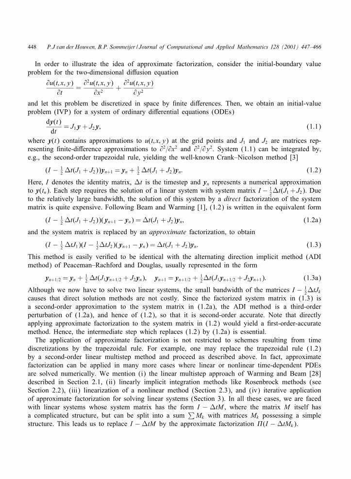
448 P.J van der Houwen, B.P. Sommeijer / Journal of Computational and Applied Mathematics 128 (2001) 447–466
In order to illustrate the idea of approximate factorization, consider the initial-boundary valueproblem for the two-dimensional di&usion equation
@u(t; x; y)@t
=@2u(t; x; y)
@x2+
@2u(t; x; y)@y2
and let this problem be discretized in space by 4nite di&erences. Then, we obtain an initial-valueproblem (IVP) for a system of ordinary di&erential equations (ODEs)
dy(t)dt
= J1y + J2y; (1.1)
where y(t) contains approximations to u(t; x; y) at the grid points and J1 and J2 are matrices rep-resenting 4nite-di&erence approximations to @2=@x2 and @2=@y2. System (1.1) can be integrated by,e.g., the second-order trapezoidal rule, yielding the well-known Crank–Nicolson method [3]
(I − 12 Lt(J1 + J2))yn+1 = yn + 1
2 Lt(J1 + J2)yn: (1.2)
Here, I denotes the identity matrix, Lt is the timestep and yn represents a numerical approximationto y(tn). Each step requires the solution of a linear system with system matrix I − 1
2 Lt(J1 + J2). Dueto the relatively large bandwidth, the solution of this system by a direct factorization of the systemmatrix is quite expensive. Following Beam and Warming [1], (1.2) is written in the equivalent form
(I − 12 Lt(J1 + J2))(yn+1 − yn) = Lt(J1 + J2)yn; (1.2a)
and the system matrix is replaced by an approximate factorization, to obtain
(I − 12 LtJ1)(I − 1
2 LtJ2)(yn+1 − yn) = Lt(J1 + J2)yn: (1.3)
This method is easily veri4ed to be identical with the alternating direction implicit method (ADImethod) of Peaceman–Rachford and Douglas, usually represented in the form
yn+1=2 = yn + 12 Lt(J1yn+1=2 + J2yn); yn+1 = yn+1=2 + 1
2 Lt(J1yn+1=2 + J2yn+1): (1.3a)
Although we now have to solve two linear systems, the small bandwidth of the matrices I − 12 LtJk
causes that direct solution methods are not costly. Since the factorized system matrix in (1.3) isa second-order approximation to the system matrix in (1.2a), the ADI method is a third-orderperturbation of (1.2a), and hence of (1.2), so that it is second-order accurate. Note that directlyapplying approximate factorization to the system matrix in (1.2) would yield a 4rst-order-accuratemethod. Hence, the intermediate step which replaces (1.2) by (1.2a) is essential.
The application of approximate factorization is not restricted to schemes resulting from timediscretizations by the trapezoidal rule. For example, one may replace the trapezoidal rule (1.2)by a second-order linear multistep method and proceed as described above. In fact, approximatefactorization can be applied in many more cases where linear or nonlinear time-dependent PDEsare solved numerically. We mention (i) the linear multistep approach of Warming and Beam [28]described in Section 2.1, (ii) linearly implicit integration methods like Rosenbrock methods (seeSection 2.2), (iii) linearization of a nonlinear method (Section 2.3), and (iv) iterative applicationof approximate factorization for solving linear systems (Section 3). In all these cases, we are facedwith linear systems whose system matrix has the form I − LtM , where the matrix M itself hasa complicated structure, but can be split into a sum
∑Mk with matrices Mk possessing a simple
structure. This leads us to replace I −LtM by the approximate factorization �(I −LtMk).
P.J van der Houwen, B.P. Sommeijer / Journal of Computational and Applied Mathematics 128 (2001) 447–466 449
In this paper, we discuss the application of the approximate factorization technique to the fourcases mentioned above and we present stability theorems for the resulting integration methods,many of which are new results. One of the results is that in the case of three-component splittingsM =
∑Mk , where the Mk have purely imaginary eigenvalues, iterative approximate factorization
leads to methods with substantial stability boundaries. Such methods are required in the numericalsolution of three dimensional, convection-dominated transport problems.
2. Noniterative factorized methods
Consider an initial-boundary-value problem for the PDE@u(t; x)
@t= L(t; x; u(t; x)); (2.1)
where L is a di&erential operator in the d-dimensional space variable x = (x1; : : : ; xd). Spatial dis-cretization yields an IVP for a system of ODEs
dy(t)dt
= f (t; y); y(t0) = y0: (2.2)
In order to simplify the notations, we shall assume that (2.2) is rewritten in autonomous form.Furthermore, it will be assumed that the Jacobian matrix J (y) := @f (y)=@y can be split into a sumof m matrices, i.e., J (y) =
∑Jk , where the splitting is either according to the spatial dimensions (as
in the early papers on splitting methods), or to the physical terms in the PDE (2.1), or accordingto any other partition leading to matrices Jk with a convenient structure. In this paper, we only usesplittings of the Jacobian and not of the right-hand side function f (y). This is often convenient inthe case of nonlinear PDEs.
We discuss three options for applying noniterative approximate factorization techniques, viz. (i)the ADI method of Warming and Beam, (ii) approximate factorization of linearly implicit integrationmethods and (iii) approximate factorization in the linearization of nonlinear methods.
2.1. The method of Warming and Beam
Consider the linear multistep method (LM method)
�(E)yn−�+1 = Lt�(E) f (yn−�+1); �(z) :=�∑
i=0
aiz�−i ; �(z) :=�∑
i=0
biz�−i ; a0 = 1; (2.3)
where E is the forward shift operator and �¿1. Warming and Beam [28] rewrite (2.3) in the form
�(E)(yn−�+1 − b0Lt f (yn−�+1)) = Lt(�(E)− b0�(E)) f (yn−�+1): (2.3a)
Since the degree of � is larger than that of � − b0�, the right-hand side does not depend on yn+1.In [28] it is assumed that f is linear, i.e., f (y) = Jy, so that (2.3a) becomes a linear system for�(E)yn−�+1. However, by replacing (2.3a) with
�(E)(yn−�+1 − b0LtJyn−�+1) = Lt(�(E)− b0�(E)) f (yn−�+1); (2.3b)
we can also deal with ODE systems where f is nonlinear (see [2]). Assuming that (2.3) is consistent,so that �(1) = 0, it can be shown that (2.3b) is an O((Lt)3) perturbation of (2.3a), and hence

450 P.J van der Houwen, B.P. Sommeijer / Journal of Computational and Applied Mathematics 128 (2001) 447–466
of (2.3). Method (2.3b) is linearly implicit in the quantity qn := �(E)yn−�+1 with system matrixI−b0LtJ = I−b0Lt
∑Jk , where I denotes the identity matrix (in the following, the identity matrix
will always be denoted by I without specifying its order, which will be clear from the context).Approximate factorization of this system matrix leads to the method of Warming and Beam:
�qn = Lt(�(E)− b0�(E)) f (yn−�+1); � :=m∏
k=1
(I − b0LtJk);
yn+1 = qn − (�(E)− E�)yn−�+1:(2.4)
Since qn = O(Lt) it follows that (2.4) is an O((Lt)3) perturbation of (2.3b) which was itself anO((Lt)3) perturbation of (2.3). Thus, if (2.3) is at least second-order accurate, then (2.4) is alsosecond-order accurate. Since the LM method (2.3) cannot be A-stable if its order is higher than twoand because A-stability of (2.3) will turn out to be a necessary condition for (2.4) to be A-stable(see Section 2.4), this order limitation is not restrictive.
If the PDE is linear and if (2.3) is de4ned by the trapezoidal rule, then (2.4) is identical to thePeaceman–Rachford method (1.3) for m = 2. Hence, (2.4) might be considered as an extension ofthe Peaceman–Rachford method (1.3) (or (1.3a)) to nonlinear PDEs with multicomponent splittings.
The computational eMciency of (2.4) depends on the structure of the successive system matricesI − b0LtJk . Let us consider the case of an m-dimensional convection-dominated problem wherethe convection terms are discretized by third-order upwind formulas. Using dimension splitting,the Jk become block-diagonal whose blocks are penta-diagonal matrices. The LU-decomposition ofI − b0LtJk and the forward=backward substitution each requires about 8N Oops for large N; Ndenoting the dimension of Jk (see, e.g., [9, p. 150]). Hence, the total costs are only proportional toN , viz. 8mN Oops per step and an additional 8mN Oops if the LU-decompositions are recomputed.Moreover, there is scope for a lot of vectorization, so that on vector computers the solution of thelinear systems in (2.4) is extremely fast. Furthermore, there is a lot of intrinsic parallelism, becauseof the block structure of Jk . However, the crucial point is the magnitude of the stepsize for whichthe method is stable. This will be the subject of Section 2.4.
Finally, we remark that the Warming–Beam method (2.4) was originally designed as an ADImethod based on dimension splitting, but it can of course be applied to any Jacobian splittingJ =
∑Jk .
2.2. Factorized linearly implicit methods
In the literature, various families of linearly implicit methods have been proposed. The 4rst meth-ods of this type are the Rosenbrock methods, proposed in 1962 by Rosenbrock [22]. A more generalfamily contains the linearly implicit Runge–Kutta methods developed by Strehmel and Weiner [26].Here, we illustrate the factorization for Rosenbrock methods which are de4ned by (cf. [11, p. 111])
yn+1 = yn + (bT ⊗ I)K ; K := (ki); i = 1; : : : ; s; n¿0;
(I−T ⊗LtJ )K = LtF(e ⊗ yn+(L⊗ I)K); J ≈ J (yn) :=@f (yn)@y
; (2.5)
where b and e are s-dimensional vectors, e has unit entries, T is an s×s diagonal or lower triangularmatrix, L is a strictly lower triangular s × s matrix, and ⊗ denotes the Kronecker or direct matrixproduct. Furthermore, for any vector V = (Ci);F(V) is de4ned by ( f (Ci)). If the order of the

P.J van der Houwen, B.P. Sommeijer / Journal of Computational and Applied Mathematics 128 (2001) 447–466 451
method (2.5) is independent of the choice of the Jacobian approximation J , then (2.5) is called aRosenbrock-W method [25]. Note that the steppoint formula in (2.5) is explicit, so that the maincomputational e&ort goes into the computation of the implicitly de4ned vector K . Since T is lowertriangular and L is strictly lower triangular, the s subsystems for ki can be solved successively.Moreover, although the system for K is nonlinear, these subsystems are linear.
Let us rewrite the system for K in the equivalent form
(I − D ⊗LtJ )K = LtF(e ⊗ yn + (L⊗ I)K) + ((T − D)⊗LtJ )K ;
where D is a diagonal matrix whose diagonal equals that of T . Then, approximately factorizing theblock-diagonal system matrix I − D ⊗LtJ = I − D ⊗Lt
∑Jk leads to the factorized Rosenbrock
method
yn+1 = yn + (bT ⊗ I)K ;
�K = LtF(e ⊗ yn + (L⊗ I)K) + ((T − D)⊗LtJ )K ; � :=m∏
k=1
(I − D ⊗LtJk):(2.6)
If the Rosenbrock method (2.5) is at least second-order accurate and if J =J (yn)+O(Lt), then (2.6)is also at least second-order accurate. However, as observed in [27], if (2.5) is a Rosenbrock-Wmethod with a diagonal matrix T with constant diagonal entries �, then the approximate factorizationdoes not a&ect the order of accuracy. This follows from the fact that for T = �I we can write� = I −�I ⊗LtJ ∗. Hence, we may consider the factorized Rosenbrock method (2.6) as the originalRosenbrock-W method with J = J ∗. Since in Rosenbrock-W methods the Jacobian can be freelychosen, Rosenbrock-W methods and their factorized versions have the same order of accuracy.
As to the computational eMciency of factorized Rosenbrock methods, we observe that if in theunderlying Rosenbrock method T =D and L=O, then the s subsystems for ki in (2.6) can be solvedconcurrently. These subsystems have the same structure as in the Warming–Beam method (2.4), sothat the computational eMciency is comparable on a parallel computer system. As an example ofsuch a parallel Rosenbrock method, we have
b =1
2(�2 − �1)
(2�2 − 1−2�1 + 1
); T =
(�1 00 �2
); L = O; �1 �= �2; (2.7)
which is second-order accurate if J = J (yn) + O(Lt).However, if either T �= D or L �= O, then the s subsystems in (2.6) have to be solved sequentially.
2.3. Approximate factorization of linearized methods
Instead of starting with a linearly implicit integration method, we may also linearize a nonlinearmethod. In fact, the Rosenbrock methods of the preceding section can be introduced by linearizingdiagonally implicit Runge–Kutta (DIRK) methods (cf. [11, p. 111]). In the literature, many otherexamples of linearization can be found. For instance, the linearization of the !-method applied tothe porus media equation (in [21, p. 203]), the linearization of the Crank–Nicolson method forhyperbolic conservation laws (in [1]) and the linearization of LM methods for the compressibleNavier–Stokes equations (in [2]). In this paper, we consider the linearization of a class of methods

452 P.J van der Houwen, B.P. Sommeijer / Journal of Computational and Applied Mathematics 128 (2001) 447–466
which contains most methods from the literature:
yn+1 = (aT ⊗ I)Yn+1 + gn; Yn+1 := (yn+ci);i = 1; : : : ; s; n¿0:
Yn+1 −Lt(T ⊗ I)F(Yn+1) = Gn; F(Yn+1) := ( f (yn+ci));(2.8)
Here, a is an s-dimensional vector and T is again an s× s matrix. The steppoint value yn+1 and thecomponents yn+ci of Yn+1 represent numerical approximations to the exact solution values y(tn + Lt)and y(tn + ciLt), where the ci are given abscissae. Yn+1 is called the stage vector, its componentsyn+ci the stage values. Gn and gn are assumed to be de4ned by preceding steppoint values yn; yn−1,etc. and by the preceding stage vectors Yn;Yn−1, etc. and their derivatives. Again, the steppointformula is explicit, so that the main computational e&ort goes into the solution of the stage vectorYn+1.
Let us linearize the stage vector equation in (2.8) to obtain for Yn+1 the linear system
Yn+1 −Lt(T ⊗ I)(F(Y 0) + (I ⊗ J )(Yn+1 − Y 0)) = Gn; J ≈ J (yn) :=@f (yn)@y
: (2.9)
Here, Y 0 is an approximation to Yn+1, for example, Y 0 = Yn or Y 0 = e ⊗ yn. However, with thissimple choice, the order of the linearized method is not necessarily the same as the original method(2.8). For instance, if (2.8) has order p¿2 and if J =J (yn)+O(Lt), then the order of the linearizedmethod is in general not higher than two. If (2.8) has order p¿3, then higher-order formulas forY 0 should be used. Of course, if the ODE system (2.2) is already linear, i.e., y′ = Jy, then Y 0 doesnot play a role, because (2.9) is identical with the stage vector equation in (2.8) for all Y 0. Notethat this also implies that the linear stability properties of (2.8) and its linearization are identical forall Y 0.
It turns out that approximate factorization of linear systems of the type (2.9) is most e&ective ifT is either diagonal or (lower) triangular as in the case of the Rosenbrock method (2.5). Therefore,from now on, we impose this condition on T . Furthermore, instead of directly applying approximatefactorization to the linear system (2.9), we 4rst rewrite it into the equivalent form (compare (1.2a))
(I −LtD ⊗ J )(Yn+1 − Y 0) = Gn − Y 0 + Lt(T ⊗ I)F(Y 0)
+ Lt((T − D)⊗ J )(Yn+1 − Y 0);(2.9a)
where again D = diag(T ). Proceeding as in the preceding section leads to the factorized method
yn+1 = (aT ⊗ I)Yn+1 + gn;
� (Yn+1 − Y 0) = Gn − Y 0 + Lt(T ⊗ I)F(Y 0) + Lt((T − D)⊗ J )(Yn+1 − Y 0)(2.10)
with � de4ned as in (2.6). If Yn+1 − Y 0 = O(Lt), then (2.10) presents a third-order perturbationof (2.9). Hence, by setting Y 0 = Yn or Y 0 = e ⊗ yn, the resulting method is second-order accurateprovided that (2.8) is also (at least) second-order accurate. We shall refer to the approximatelyfactorized, linearized method (2.10) as the AFL method.
If T is diagonal, then the subsystems for the components of Yn+1−Y 0 can be solved concurrently,and if T is lower triangular, then these subsystems should be solved successively (note that T − D
P.J van der Houwen, B.P. Sommeijer / Journal of Computational and Applied Mathematics 128 (2001) 447–466 453
is strictly lower triangular). The computational eMciency of solving the linear systems in (2.10) iscomparable with that of (2.6).
2.4. Stability
As already remarked, the crucial point is the stability of the factorized methods. We shall discussstability with respect to the model problem y′ = Jy =
∑Jky, where the matrices Jk commute.
Application of the factorized methods to this model problem leads to linear recursions. The roots $of the corresponding characteristic equations de4ne the ampli>cation factors of the method. Theseampli4cation factors are functions of the vector z=(z1; : : : ; zm)T, where zk runs through the eigenvaluesof LtJk . We call a method stable at the point z if its ampli4cation factor $(z) is on the unit disk.Likewise, we shall call a function R(z) stable at z if R(z) is on the unit disk. In the stabilityde4nitions and stability theorems given below, we shall use the notation
W(&) := {w ∈ C: |arg(−w)|6&};R(() := (−(; 0];
I(() :={w ∈ C: arg(w) =±�
2; |w|¡(
}:
De�nition 2.1. A method or a function is called
• A(&)-stable if it is stable for zk ∈W(&); k = 1; : : : ; m,• A-stable if it is stable for zk ∈W(�=2); k = 1; : : : ; m,• Ar(&)-stable if it is stable for z1; : : : ; zr ∈ R(∞) ∧ zr+1; : : : ; zm ∈W(&).
The 4rst two de4nitions of stability are in analogy with the de4nitions in numerical ODE theory. Thethird type of stability was introduced by Hundsdorfer [17] and will be referred to as Ar(&)-stability.This type of stability is relevant in the case of convection–di&usion–reaction equations. For example,for systems of two-dimensional convection–di&usion–reaction equations in which the Jacobian of thereaction terms has real, sti& eigenvalues, we would like to have A1(�=2)-stability for m = 3, thatis, stability in the region R(∞) ×W(�=2) ×W(�=2). Then, by choosing the splitting such that J1
corresponds to the reaction terms, and J2 and J3 to the convection–di&usion terms in the two spatialdirections, we achieve unconditional stability. We remark that in the case of a single two-dimensionalconvection–di&usion–reaction equation, we need only A-stability for m = 2, because we can choosethe splitting such that J1 corresponds to the reaction term and the convection–di&usion in one spatialdirection, and J2 to convection–di&usion in the other spatial direction. Note that in this splitting, thematrices J1 and J2 both have a band structure with small band width.
In the following, we shall often encounter stability regions containing subregions of the formS1 × S2 × S3. In the case of approximate factorizations that are symmetric with respect to theJacobians J1; J2 and J3, as in the methods (2.4), (2.6) and (2.10), this means that the stability regionalso contains the subregions S1 × S3 × S2; S2 × S1 × S3; : : : :
In the next sections, we give stability theorems for the method of Warming and Beam, and a fewAFL and factorized Rosenbrock methods.

454 P.J van der Houwen, B.P. Sommeijer / Journal of Computational and Applied Mathematics 128 (2001) 447–466
2.5. Method of Warming and Beam
Applying the Warming–Beam method (2.4) to the stability test problem yields the followingcharacteristic equation for the ampli4cation factor $ = $(z) of the method:
�($)− (z)�($) = 0; (z) := eTz
[b0eTz +
m∏k=1
(1− b0zk)
]−1
: (2.11)
Stability properties of (2.4) can be derived by using the following lemma of Hundsdorfer [17]:
Lemma 2.2. Let Hm be the function de>ned by
Hm(w) := 1 + eTwm∏
k=1
(1− 12wk)−1; w = (w1; : : : ; wm)T; m¿2:
Hm is A(&)-stable if and only if &6 12�(m− 1)−1 and Ar(&)-stable if and only if &6 1
2�(m− r)−1.
Theorem 2.3. Let the LM method (2:3) be A-stable. Then the Warming–Beam method (2:4) is(a) A(&)-stable for m¿2 if and only if &6 1
2�(m− 1)−1.(b) Ar(&)-stable for m¿2 and r¿1 if and only if &6 1
2�(m− r)−1.(c) Stable in the region I((1)× I((1)× R((2) for m = 3 if b2
0(21(b0(2 − 3) = 1.
Proof. If the method (2.3) is A-stable, then (2.4) is stable at the point z if Re( (z))60, or equiv-alently, if |(1 + c (z))(1 − c (z))−1|61 for some positive constant c. Let us choose c = b0 (theA-stability of (2.3) implies that b0 ¿ 0). Then, it follows from (2.11) that
1 + b0 (z)1− b0 (z)
= Hm(2b0z); (2.12)
where Hm is de4ned in Lemma 2.2. Applying this lemma with w = 2b0z proves part (a) and (b).Part (c) is proved by analysing the inequality |H (2b0z)|61 for z= (iy1; iy2; x3). For m= 3 this leadsto
((1− b20y1y2)(1− b0x3) + 2b0x3)2 + (b0(y1 + y2)(1 + b0x3))2
6(1 + b20y
21)(1 + b2
0y22)(1− b0x3)2:
The most critical situation is obtained if y1 and y2 assume their maximal value. Setting y1 =y2 =(1
and taking into account that x360, the inequality reduces to x3¿ − (1 + 3b20(
21)=b3
0(21 from which
assertion (c) is immediate.
This theorem implies A-stability for m = 2, a result already obtained by Warming and Beam[28]. Furthermore, the theorem implies A(0)-stability for all m¿2, and A(&)-stability with &6�=4for m¿3. Hence, we do not have unconditional stability in the case where all Jacobians Jk haveeigenvalues close to the imaginary axis. We even do not have stability in regions of the formI(() × I(() × I(() or I(() × I(() × R(∞) with (¿ 0 (see also [12]). However, part (c) of thetheorem implies for m = 3 stability in W(�=2) ×W(�=2) × R(3=b0). Such regions are suitable forsystems of two-dimensional convection–di&usion–reaction equations with real, nonsti@ eigenvalues
P.J van der Houwen, B.P. Sommeijer / Journal of Computational and Applied Mathematics 128 (2001) 447–466 455
in the reaction part. Note that it is advantageous to use small b0-values, whereas L-stability of theunderlying LM method does not lead to better stability properties.
Remark 2.4. The ampli4cation factors of the stabilizing corrections method of Douglas (cf. [6,7])are given by $ = H (z), so that it has similar stability properties as the Warming–Beam method.
Remark 2.5. As already remarked in Section 2.1, (2.4) can be seen as a generalization of thePeaceman–Rachford method (1.3) to nonlinear PDEs with multicomponent splittings. In the literature,a second, direct generalization of (1.3a) is known, however its stability is less satisfactory. For thede4nition of this generalization, let F be a splitting function with m arguments satisfying the relationF(y; : : : ; y)=f (y) and de4ne Fk by setting the kth argument of F equal to yk and all other argumentsequal to yk−1. Then, the direct generalization of (1.3a) reads
y0 = yn; yk = yk−1 +Ltm
Fk ; yn+1 = ym; k = 1; : : : ; m
(cf., e.g., [19, p. 278] and [16]). This scheme is second-order accurate for all F . Evidently, it reducesto (1.3a) for linear problems and m = 2. Its ampli4cation factor is given by
$(z) =m∏
k=1
m + eTz − zkm− zk
;
showing that unlike the Warming–Beam method, it is not even A(0)-stable for m¿3 (e.g., $(ez0) ≈(1− m)m as z0 →∞), so that it is only of use for m = 2.
2.6. AFL–LM methods
We start with AFL methods based on the class of LM methods (2.3). Writing (2.3) in the form(2.8) and applying the AFL method (2.10) to the stability test problem leads to the characteristicequation
�($)− eTz�($) =
[1− b0eTz −
m∏k=1
(1− b0zk)
]($− 1)$�−1: (2.13)
This equation does not allow such a general stability analysis as in the case (2.11). Therefore, wecon4ne our considerations to two particular cases, viz. the AFL methods based on the trapezoidalrule and the BDF method.
2.6.1. The trapezoidal ruleThe trapezoidal rule is de4ned by �($) = $ − 1; �($) = 1
2 ($ + 1). This leads to the characteristicequation $=H (z), where H is de4ned in Lemma 2.2. Hence, according to the proof of Theorem 2.3the AFL-trapezoidal rule and the Warming–Beam method with b0 = 1
2 possess the same stabilityregion, so that Theorem 2.3 applies (with b0 = 1
2 in part (c)).

456 P.J van der Houwen, B.P. Sommeijer / Journal of Computational and Applied Mathematics 128 (2001) 447–466
2.6.2. The BDF methodFor the BDF with �($) = $2 − 4
3$ + 13 ; �($) = 2
3$2 the characteristic equation (2.13) assumes the
form
$2 − C1$ + C2 = 0;
C1 =P(z)Q(z)
; C2 =1
Q(z); P(z) :=Q(z) + 1 + 2eTz; Q(z) := 3
m∏k=1
(1− 23zk):
(2.14)
In order to 4nd the stability region, we use Schur’s criterion stating that the ampli4cation factorsare on the unit disk if |C2|2 + |C1 − C∗
1 C2|61 .
Theorem 2.6. The AFL–BDF method is A-stable for m = 2 and A(�=4)-stable for m = 3.
Proof. Let P∗ and Q∗ denote the complex conjugates of P and Q. Then, in terms of P and Q, theSchur criterion requires that the function R(z) := |(P(z)Q∗(z)−P∗(z))=(Q(z)Q∗(z)− 1)| is boundedby one in the product space de4ned by Re zk ¡ 0; k = 1; : : : ; m. Since |1− 2
3zk |2 ¿ 1 for zk in the lefthalf-plane, we easily see that R(z) is analytic in this product space. Hence, the maximum principlereveals that we need to require |R(iy1; : : : ; iym)|61, where we have written zk = iyk , with yk real.This condition on its own is equivalent to requiring that the polynomial E(iy) := (|Q(iy)|2 − 1)2 −|P(iy)Q∗(iy)− P∗(iy)|2 with y := (y1; : : : ; ym)T is nonnegative. For m = 2 we straightforwardly 4ndthat
E(iy1; iy2) = 169 (y1 + y2)2(9y2
1 + 9y22 + 4y2
1y22 + 6y1y2):
It is easily seen that E(iy1; iy2)¿0 for all y1 and y2, proving the A-stability for m = 2.For m = 3 we set zk = xk − ixk ; k = 1; 2; 3, with xk60 and derived an expression for E(z) with
the help of Maple. This expression has the form −eTxs(x), where x = (x1; x2; x3)T and s(x) consistsof a sum of terms each term being of the form xp
1 xq2x
r3, where p; q and r are nonnegative integers.
We veri4ed that the coeMcients of these terms are all positive if p + q + r is even and negativeotherwise (the length of the formulas prevents us from presenting s(x) here). Hence, E(z)¿0 forall zk = xk − ixk with xk60. Likewise, it can be shown that E(z)¿0 for all zk = xk + ixk with xk60,proving the A(�=4)-stability for m = 3.
In addition, we determined stability regions of the form I((1) × I((1) × R((2) by analysing thestability boundary curve E(iy1; iy2; x3)=0 with the help of Maple. In particular, we found that in theregion W(�=2)×W(�=2)×R(() the value of ( is determined by the equation E(i∞; i∞; () = 0 andin the region I(()×I(()×R(∞) by the equation E(i(; i(;∞)=0. This leads to (=(9+3
√17)=4 and
(= 34
√2, respectively. For the sake of easy comparison, we have listed a number of stability results
derived in this paper in Table 1. This table shows that the AFL–BDF regions I(()×I(()×R(∞) andW(�=2)×W(�=2)×R(() are larger than the corresponding stability regions of the Warming–Beammethod generated by the BDF (b0 = 2
3 ). We now even have stability in I(() × I(() × I(() withnonzero imaginary stability boundary (, however these boundaries are quite small ((¡ 1=10).
P.J van der Houwen, B.P. Sommeijer / Journal of Computational and Applied Mathematics 128 (2001) 447–466 457
2.7. AFL–DIRK methods
If we de4ne in (2.8) gn = (1− aTe)yn and Gn = e⊗ yn, then (2.8) becomes a diagonally implicitRunge–Kutta (DIRK) method. We de4ne an AFL–DIRK method by approximating Yn+1 by meansof (2.10) with Y 0 = e⊗ yn. The ampli4cation factor with respect to the stability test model becomes
$(z) = 1 + eTzaT
(m∏
k=1
(I − zkD)− eTz(T − D)
)−1
Te: (2.15)
Let us consider the second-order, L-stable DIRK methods
yn+1 = (eT2 ⊗ I)Yn+1; Yn+1 =
(yn+�
yn+1
);
Yn+1 −Lt(T ⊗ I)F(Yn+1) = e ⊗ yn; T =(
� 01− � �
) (2.16a)
and
yn+1 = (1− aTe)yn + aTYn+1; Yn+1 =(
yn+�
yn+1−�
); a =
12�2
(3� − 1
�
);
Yn+1 −Lt(T ⊗ I)F(Yn+1) = e ⊗ yn; T =(
� 01− 2� �
);
(2.16b)
where e2 = (0; 1)T and � = 1± 12
√2. The ampli4cation factor (2.15) becomes in both cases
$(z) = 1 +eTz�(z)
+�(1− �)(eTz)2
�2(z); �(z) :=
m∏k=1
(1− �zk); � = 1± 12
√2: (2.17)
Theorem 2.7. The AFL versions of (2:16) are A-stable for m = 2 and A(�=4)-stable for m = 3.
Proof. Writing $(z)=P(z)Q−1(z), where P and Q are polynomials in z1; z2 and z3, it follows that wehave A-stability if the E-polynomial E(z) := |Q(z)|2−|P(z)|2 is nonnegative for all purely imaginaryzk . Using Maple, we found for � = 1± 1
2
√2
E(iy1; iy2; 0) = 14 (17± 12
√2)(y1 + y2)4;
which proves the A-stability for m = 2. Similarly, the A(�=4) stability can be shown for m = 3.
Thus, the A-stability and A(&)-stability properties of the Warming–Beam, AFL-trapezoidal, AFL–BDF, and the above AFL–DIRK methods are comparable for m63. However, for the AFL–DIRKmethods we found (numerically) the stability regions I((1)×I((1)×R(∞) and W(�=2)×W(�=2)×R((2) with (1 ≈ 1:26 and (2 ≈ 10:2 for � = 1 − 1
2
√2 and with (1 ≈ 0:28 and (2 ≈ 1:75 for
� = 1 + 12
√2. Hence, choosing � = 1− 1
2
√2 we have larger stability regions than the corresponding
stability regions of the other methods (see Table 1). We also have stability in regions of the typeI(()× I(()× I(() with (¿ 0, but ( is uselessly small.
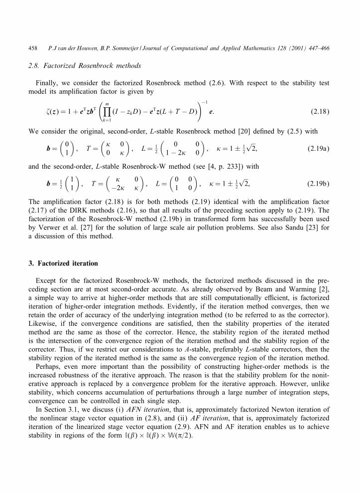
458 P.J van der Houwen, B.P. Sommeijer / Journal of Computational and Applied Mathematics 128 (2001) 447–466
2.8. Factorized Rosenbrock methods
Finally, we consider the factorized Rosenbrock method (2.6). With respect to the stability testmodel its ampli4cation factor is given by
$(z) = 1 + eTzbT
(m∏
k=1
(I − zkD)− eTz(L + T − D)
)−1
e: (2.18)
We consider the original, second-order, L-stable Rosenbrock method [20] de4ned by (2.5) with
b =(
01
); T =
(� 00 �
); L = 1
2
(0 0
1− 2� 0
); � = 1± 1
2
√2; (2.19a)
and the second-order, L-stable Rosenbrock-W method (see [4, p. 233]) with
b = 12
(11
); T =
(� 0−2� �
); L =
(0 01 0
); � = 1± 1
2
√2; (2.19b)
The ampli4cation factor (2.18) is for both methods (2.19) identical with the ampli4cation factor(2.17) of the DIRK methods (2.16), so that all results of the preceding section apply to (2.19). Thefactorization of the Rosenbrock-W method (2.19b) in transformed form has successfully been usedby Verwer et al. [27] for the solution of large scale air pollution problems. See also Sandu [23] fora discussion of this method.
3. Factorized iteration
Except for the factorized Rosenbrock-W methods, the factorized methods discussed in the pre-ceding section are at most second-order accurate. As already observed by Beam and Warming [2],a simple way to arrive at higher-order methods that are still computationally eMcient, is factorizediteration of higher-order integration methods. Evidently, if the iteration method converges, then weretain the order of accuracy of the underlying integration method (to be referred to as the corrector).Likewise, if the convergence conditions are satis4ed, then the stability properties of the iteratedmethod are the same as those of the corrector. Hence, the stability region of the iterated methodis the intersection of the convergence region of the iteration method and the stability region of thecorrector. Thus, if we restrict our considerations to A-stable, preferably L-stable correctors, then thestability region of the iterated method is the same as the convergence region of the iteration method.
Perhaps, even more important than the possibility of constructing higher-order methods is theincreased robustness of the iterative approach. The reason is that the stability problem for the nonit-erative approach is replaced by a convergence problem for the iterative approach. However, unlikestability, which concerns accumulation of perturbations through a large number of integration steps,convergence can be controlled in each single step.
In Section 3.1, we discuss (i) AFN iteration, that is, approximately factorized Newton iteration ofthe nonlinear stage vector equation in (2.8), and (ii) AF iteration, that is, approximately factorizediteration of the linearized stage vector equation (2.9). AFN and AF iteration enables us to achievestability in regions of the form I(()× I(()×W(�=2).
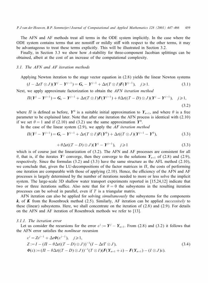
P.J van der Houwen, B.P. Sommeijer / Journal of Computational and Applied Mathematics 128 (2001) 447–466 459
The AFN and AF methods treat all terms in the ODE system implicitly. In the case where theODE system contains terms that are nonsti& or mildly sti& with respect to the other terms, it maybe advantageous to treat these terms explicitly. This will be illustrated in Section 3.2.
Finally, in Section 3.3 we show how A-stability for three-component Jacobian splittings can beobtained, albeit at the cost of an increase of the computational complexity.
3.1. The AFN and AF iteration methods
Applying Newton iteration to the stage vector equation in (2.8) yields the linear Newton systems
(I −LtT ⊗ J )(Y j − Y j−1) = Gn − Y j−1 + Lt(T ⊗ I)F(Y j−1); j¿1: (3.1)
Next, we apply approximate factorization to obtain the AFN iteration method
�(Y j − Y j−1) = Gn − Y j−1 + Lt(T ⊗ I)F(Y j−1) + !Lt((T − D)⊗ J )(Y j − Y j−1); j¿1;
(3.2)
where � is de4ned as before, Y 0 is a suitable initial approximation to Yn+1, and where ! is a freeparameter to be explained later. Note that after one iteration the AFN process is identical with (2.10)if we set ! = 1 and if (2.10) and (3.2) use the same approximation Y 0.
In the case of the linear system (2.9), we apply the AF iteration method
�(Y j − Y j−1) = Gn − Y j−1 + Lt(T ⊗ I)F(Y 0) + Lt((T ⊗ J )(Y j−1 − Y 0); (3.3)
+ !Lt((T − D)⊗ J )(Y j − Y j−1); j¿1 (3.3)
which is of course just the linearization of (3.2). The AFN and AF processes are consistent for all!, that is, if the iterates Y j converge, then they converge to the solutions Yn+1 of (2.8) and (2.9),respectively. Since the formulas (3.2) and (3.3) have the same structure as the AFL method (2.10),we conclude that, given the LU-decompositions of the factor matrices in �, the costs of performingone iteration are comparable with those of applying (2.10). Hence, the eMciency of the AFN and AFprocesses is largely determined by the number of iterations needed to more or less solve the implicitsystem. The large-scale 3D shallow water transport experiments reported in [15,24,12] indicate thattwo or three iterations suMce. Also note that for ! = 0 the subsystems in the resulting iterationprocesses can be solved in parallel, even if T is a triangular matrix.
AFN iteration can also be applied for solving simultaneously the subsystems for the componentski of K from the Rosenbrock method (2.5). Similarly, AF iteration can be applied successively tothese (linear) subsystems. Here, we shall concentrate on the iteration of (2.8) and (2.9). For detailson the AFN and AF iteration of Rosenbrock methods we refer to [13].
3.1.1. The iteration errorLet us consider the recursions for the error 3 j :=Y j − Yn+1. From (2.8) and (3.2) it follows that
the AFN error satis4es the nonlinear recursion
3 j = Z3j−1 + Lt5(3 j−1); j¿1;
Z := I − (� − !Lt((T − D)⊗ J ))−1(I −LtT ⊗ J ); (3.4)
5(3) := (� − !Lt((T − D)⊗ J ))−1(T ⊗ I)(F(Yn+1 + 3)− F(Yn+1)− (I ⊗ J )3):

460 P.J van der Houwen, B.P. Sommeijer / Journal of Computational and Applied Mathematics 128 (2001) 447–466
Similarly, we deduce from (2.9) and (3.3) for the AF error the linear recursion
3 j = Z3j−1; j¿1: (3.5)
It is diMcult to decide which of the two iteration processes has a better rate of convergence. However,in a 4rst approximation, the rates of convergence are comparable, because in the neighbourhoodof the origin the Lipschitz constant of the function 5 is quite small, provided that J is a closeapproximation to J (yn). Therefore, we will concentrate on the ampli4cation matrix Z .
First of all, we consider the convergence for small Lt. Since Z =(1−!)Lt(T−D)⊗J +O((Lt)2),the following theorem is easily proved (cf. [13]):
Theorem 3.1. The iteration errors of the AFN and AF iteration processes (3:2) and (3:3) satisfy
3 j = O((Lt)2j)30; j¿1 if T is diagonal or if ! = 1;
3 j ={
O((Lt)j)30 for 16j6s− 1O((Lt)2j+1−s)30 for j¿s
if T is lower triangular and ! �= 1:
This theorem shows that we always have convergence if Lt is suMciently small. It also indicatesthat the nonsti& error components (corresponding with eigenvalues of Jk of modest magnitude) arerapidly removed from the iteration error. Furthermore, we now see the price to be paid if we set! = 0, while T is lower triangular (and not diagonal). In such cases, the subsystems in (3.2) and(3.3) can still be solved in parallel, however, at the cost of a lower order of convergence.
3.1.2. Convergence and stability regionsThe eigenvalues 6(Z) of the ampli4cation matrix Z will be called the ampli>cation factors in
the iteration process. As in the stability analysis, we consider the test equation where the Jacobianmatrices Jk commute. For this model problem, they are given by the eigenvalues of the matrixI −�−1(I −LtT ⊗ J ), so that
6(Z) = 1− (1− 6(T )eTz)m∏
k=1
(1− 6(T )zk)−1:
Note that 6(Z) does not depend on the parameter !. We shall call a method convergent at z if 6(Z)is within the unit circle at z. This leads us to the following analogue of De4nition 2.1.
De�nition 3.2. The iteration method is called
• A(&)-convergent if it is convergent for zk ∈W(&); k = 1; : : : ; m,• A-convergent if it is convergent for zk ∈W(�=2); k = 1; : : : ; m,• Ar(&)-convergent if it is convergent for z1; : : : ; zr ∈ R(∞) ∧ zr+1; : : : ; zm ∈W(&).
From now on, we shall explicitly assume that
the corrector method is A-stable or L-stable;the matrix T has nonnegative eigenvalues;the iteration process is performed until convergence:
(3.6)
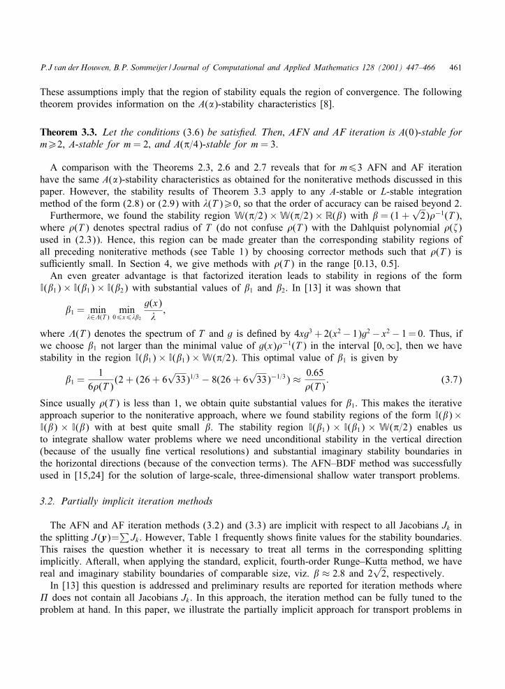
P.J van der Houwen, B.P. Sommeijer / Journal of Computational and Applied Mathematics 128 (2001) 447–466 461
These assumptions imply that the region of stability equals the region of convergence. The followingtheorem provides information on the A(&)-stability characteristics [8].
Theorem 3.3. Let the conditions (3.6) be satis>ed. Then; AFN and AF iteration is A(0)-stable form¿2, A-stable for m = 2; and A(�=4)-stable for m = 3.
A comparison with the Theorems 2.3, 2.6 and 2.7 reveals that for m63 AFN and AF iterationhave the same A(&)-stability characteristics as obtained for the noniterative methods discussed in thispaper. However, the stability results of Theorem 3.3 apply to any A-stable or L-stable integrationmethod of the form (2.8) or (2.9) with 6(T )¿0, so that the order of accuracy can be raised beyond 2.
Furthermore, we found the stability region W(�=2)×W(�=2)× R(() with ( = (1 +√
2)�−1(T ),where �(T ) denotes spectral radius of T (do not confuse �(T ) with the Dahlquist polynomial �($)used in (2.3)). Hence, this region can be made greater than the corresponding stability regions ofall preceding noniterative methods (see Table 1) by choosing corrector methods such that �(T ) issuMciently small. In Section 4, we give methods with �(T ) in the range [0.13, 0.5].
An even greater advantage is that factorized iteration leads to stability in regions of the formI((1)× I((1)× I((2) with substantial values of (1 and (2. In [13] it was shown that
(1 = min6∈7(T )
min06x66(2
g(x)6
;
where 7(T ) denotes the spectrum of T and g is de4ned by 4xg3 + 2(x2− 1)g2− x2− 1 = 0. Thus, ifwe choose (1 not larger than the minimal value of g(x)�−1(T ) in the interval [0;∞], then we havestability in the region I((1)× I((1)×W(�=2). This optimal value of (1 is given by
(1 =1
6�(T )(2 + (26 + 6
√33)1=3 − 8(26 + 6
√33)−1=3) ≈ 0:65
�(T ): (3.7)
Since usually �(T ) is less than 1, we obtain quite substantial values for (1. This makes the iterativeapproach superior to the noniterative approach, where we found stability regions of the form I(()×I(() × I(() with at best quite small (. The stability region I((1) × I((1) ×W(�=2) enables usto integrate shallow water problems where we need unconditional stability in the vertical direction(because of the usually 4ne vertical resolutions) and substantial imaginary stability boundaries inthe horizontal directions (because of the convection terms). The AFN–BDF method was successfullyused in [15,24] for the solution of large-scale, three-dimensional shallow water transport problems.
3.2. Partially implicit iteration methods
The AFN and AF iteration methods (3.2) and (3.3) are implicit with respect to all Jacobians Jk inthe splitting J (y)=
∑Jk . However, Table 1 frequently shows 4nite values for the stability boundaries.
This raises the question whether it is necessary to treat all terms in the corresponding splittingimplicitly. Afterall, when applying the standard, explicit, fourth-order Runge–Kutta method, we havereal and imaginary stability boundaries of comparable size, viz. ( ≈ 2:8 and 2
√2, respectively.
In [13] this question is addressed and preliminary results are reported for iteration methods where� does not contain all Jacobians Jk . In this approach, the iteration method can be fully tuned to theproblem at hand. In this paper, we illustrate the partially implicit approach for transport problems in
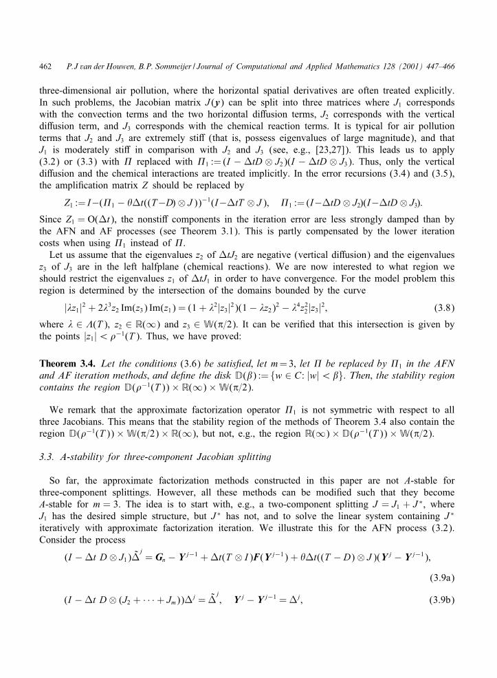
462 P.J van der Houwen, B.P. Sommeijer / Journal of Computational and Applied Mathematics 128 (2001) 447–466
three-dimensional air pollution, where the horizontal spatial derivatives are often treated explicitly.In such problems, the Jacobian matrix J (y) can be split into three matrices where J1 correspondswith the convection terms and the two horizontal di&usion terms, J2 corresponds with the verticaldi&usion term, and J3 corresponds with the chemical reaction terms. It is typical for air pollutionterms that J2 and J3 are extremely sti& (that is, possess eigenvalues of large magnitude), and thatJ1 is moderately sti& in comparison with J2 and J3 (see, e.g., [23,27]). This leads us to apply(3.2) or (3.3) with � replaced with �1 := (I − LtD ⊗ J2)(I − LtD ⊗ J3). Thus, only the verticaldi&usion and the chemical interactions are treated implicitly. In the error recursions (3.4) and (3.5),the ampli4cation matrix Z should be replaced by
Z1 := I−(�1 − !Lt((T−D)⊗ J ))−1(I−LtT ⊗ J ); �1 := (I−LtD ⊗ J2)(I−LtD ⊗ J3):
Since Z1 = O(Lt), the nonsti& components in the iteration error are less strongly damped than bythe AFN and AF processes (see Theorem 3.1). This is partly compensated by the lower iterationcosts when using �1 instead of �.
Let us assume that the eigenvalues z2 of LtJ2 are negative (vertical di&usion) and the eigenvaluesz3 of J3 are in the left halfplane (chemical reactions). We are now interested to what region weshould restrict the eigenvalues z1 of LtJ1 in order to have convergence. For the model problem thisregion is determined by the intersection of the domains bounded by the curve
|6z1|2 + 263z2 Im(z3) Im(z1) = (1 + 62|z3|2)(1− 6z2)2 − 64z22|z3|2; (3.8)
where 6 ∈ 7(T ); z2 ∈ R(∞) and z3 ∈W(�=2): It can be veri4ed that this intersection is given bythe points |z1|¡�−1(T ). Thus, we have proved:
Theorem 3.4. Let the conditions (3.6) be satis>ed; let m= 3; let � be replaced by �1 in the AFNand AF iteration methods; and de>ne the disk D(() := {w ∈ C: |w|¡(}. Then; the stability regioncontains the region D(�−1(T ))× R(∞)×W(�=2).
We remark that the approximate factorization operator �1 is not symmetric with respect to allthree Jacobians. This means that the stability region of the methods of Theorem 3.4 also contain theregion D(�−1(T ))×W(�=2)× R(∞); but not, e.g., the region R(∞)×D(�−1(T ))×W(�=2).
3.3. A-stability for three-component Jacobian splitting
So far, the approximate factorization methods constructed in this paper are not A-stable forthree-component splittings. However, all these methods can be modi4ed such that they becomeA-stable for m = 3. The idea is to start with, e.g., a two-component splitting J = J1 + J ∗, whereJ1 has the desired simple structure, but J ∗ has not, and to solve the linear system containing J ∗
iteratively with approximate factorization iteration. We illustrate this for the AFN process (3.2).Consider the process
(I −Lt D ⊗ J1)Lj
= Gn − Y j−1 + Lt(T ⊗ I)F(Y j−1) + !Lt((T − D)⊗ J )(Y j − Y j−1);
(3.9a)
(I −Lt D ⊗ (J2 + · · ·+ Jm))Lj = Lj; Y j − Y j−1 = Lj; (3.9b)

P.J van der Houwen, B.P. Sommeijer / Journal of Computational and Applied Mathematics 128 (2001) 447–466 463
where j¿1. This method can be interpreted as the AFN method (3.2) with m replaced by 2 andJ2 replaced by J2 + · · · + Jm. Hence, Theorem 3.3 implies that we have A-stability with respectto the eigenvalues of J1 and J2 + · · · + Jm (assuming that the corrector is A-stable). If the matrixJ2 + · · · + Jm does not have a ‘convenient’ structure (e.g., a small band width), then the systemfor Lj cannot be solved eMciently. In such cases, we may solve this system by an AFN (inner)iteration process:
Lj;0 = Lj;
�1(Lj; i −Lj; i−1) = Lj − (I −Lt D ⊗ (J2 + · · ·+ Jm))Lj; i−1; i = 1; : : : ; r; (3.9c)
Y j = Y j−1 + Lj; r ; �1 :=m∏
k=2
(I −Lt D ⊗ Jk):
Since the stability theory of Section 3.1 applies to this process, we can apply the stability resultsfrom this section. The following theorem summarizes the main results for {(3.9a),(3.9c)}.
Theorem 3.5. Let (3.6) be satis>ed. Then; the inner-outer AFN process {(3:9a); (3:9c)} is
(a) A(0)-stable for m¿2; A-stable for m = 2 and m = 3; and A(�=4)-stable for m = 4;(d) Stable in W(�=2)× I(()× I(()×W(�=2) with ( ≈ 0:65 �−1(T ) for m = 4;(e) Stable in W(�=2)×W(�=2)×W(�=2)× R(() with ( = (1 +
√2) �−1(T ) for m = 4.
Thus the process {(3.9a),(3.9c)} has excellent stability properties, but its computational complexityis considerably larger than that of (3.2). In order to compare this, let the number of outer iterationsbe denoted by q. Then (3.2) requires the solution of qm linear systems, whereas {(3.9a),(3.9c)}requires q(rm + 1 − r) linear system solutions. For example, if m = 3, then we need 3q and(2r + 1)q linear system solutions, respectively, so that for r¿2 the nested approach is more expen-sive.
Evidently, the above approach can also be applied to the AF method (3.3), but also to the nonit-erative methods (2.4), (2.6), and (2.10). In the noniterative methods, the computational complexityincreases from m to rm + 1 − r linear system solutions, i.e., by the same factor as in the iterativecase. It should be remarked that there exist several splitting methods, not based on approximatefactorization, that are also A-stable for three-component Jacobian splittings. We mention the ADImethod of Gourlay and Mitchell [10] and the trapezoidal and midpoint splitting methods of Hunds-dorfer [18]. These methods are second-order accurate and possess the same ampli4cation factor$(z) =
∏3k=1(1 + 1
2zk)(1 − 12zk)
−1 from which the A-stability is immediate. However, the internalstages of these methods are not consistent, that is, in a steady state the internal stage values are notstationary points of the method. This leads to loss of accuracy (cf. [17]).
4. Methods with minimal �(T)
The stability regions in Table 1 and the Theorems 3.4 and 3.5 indicate that small values of �(T )increase the stability regions of the iterated methods. Similarly, Theorem 2.3 shows that small values
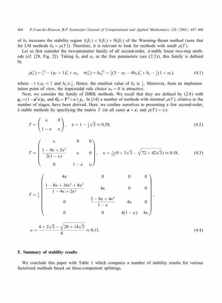
464 P.J van der Houwen, B.P. Sommeijer / Journal of Computational and Applied Mathematics 128 (2001) 447–466
of b0 increases the stability region I((1)× I((1)× R((2) of the Warming–Beam method (note thatfor LM methods b0 = �(T )): Therefore, it is relevant to look for methods with small �(T ).
Let us 4rst consider the two-parameter family of all second-order, A-stable linear two-step meth-ods (cf. [28, Fig. 2]). Taking b0 and a2 as the free parameters (see (2.3)), this family is de4nedby
�($) = $2 − (a2 + 1)$ + a2; �($) = b0$2 + 12 (3− a2 − 4b0)$ + b0 − 1
2 (1 + a2); (4.1)
where −16a2 ¡ 1 and b0¿ 12 . Hence, the smallest value of b0 is 1
2 . Moreover, from an implemen-tation point of view, the trapezoidal rule choice a2 = 0 is attractive.
Next, we consider the family of DIRK methods. We recall that they are de4ned by (2.8) withgn=(1−aTe)yn and Gn=Y 0 =e⊗yn. In [14] a number of methods with minimal �(T ), relative to thenumber of stages, have been derived. Here, we con4ne ourselves to presenting a few second-order,L-stable methods by specifying the matrix T (in all cases a = es and �(T ) = �):
T =
� 0
1− � �
; � = 1− 1
2
√2 ≈ 0:29; (4.2)
T =
� 0 0
1− 4� + 2�2
2(1− �)� 0
0 1− � �
; � = 1
12 (9 + 3√
3−√
72 + 42√
3) ≈ 0:18; (4.3)
T = 14
4� 0 0 0
1− 8� + 16�2 + 8�3
1− 4� + 2�24� 0 0
02− 8� + 4�2
1− �4� 0
0 0 4(1− �) 4�
;
� =4 + 2
√2−
√20 + 14
√2
4≈ 0:13: (4.4)
5. Summary of stability results
We conclude this paper with Table 1 which compares a number of stability results for variousfactorized methods based on three-component splittings.
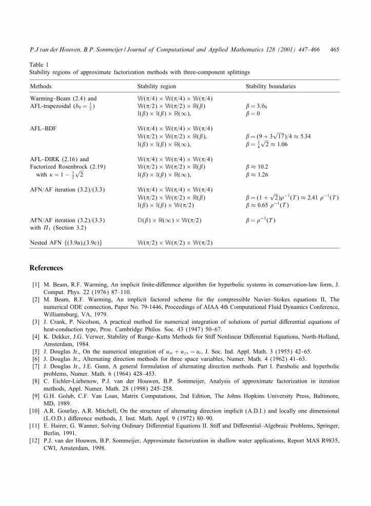
P.J van der Houwen, B.P. Sommeijer / Journal of Computational and Applied Mathematics 128 (2001) 447–466 465
Table 1Stability regions of approximate factorization methods with three-component splittings
Methods Stability region Stability boundaries
Warming–Beam (2.4) and W(�=4) ×W(�=4) ×W(�=4)AFL-trapezoidal (b0 = 1
2 ) W(�=2) ×W(�=2) × R(() ( = 3=b0
I(() × I(() × R(∞); ( = 0
AFL–BDF W(�=4) ×W(�=4) ×W(�=4)W(�=2) ×W(�=2) × R((); ( = (9 + 3
√17)=4 ≈ 5:34
I(() × I(() × R(∞); ( = 34
√2 ≈ 1:06
AFL–DIRK (2.16) and W(�=4) ×W(�=4) ×W(�=4)Factorized Rosenbrock (2.19) W(�=2) ×W(�=2) × R(() ( ≈ 10:2
with � = 1 − 12
√2 I(() × I(() × R(∞), ( ≈ 1:26
AFN=AF iteration (3.2)=(3.3) W(�=4) ×W(�=4) ×W(�=4)W(�=2) ×W(�=2) × R(() ( = (1 +
√2)�−1(T ) ≈ 2:41 �−1(T )
I(() × I(() ×W(�=2) ( ≈ 0:65 �−1(T )
AFN=AF iteration (3.2)=(3.3) D(() × R(∞) ×W(�=2) ( = �−1(T )with �1 (Section 3:2)
Nested AFN {(3.9a),(3.9c)} W(�=2) ×W(�=2) ×W(�=2)
References
[1] M. Beam, R.F. Warming, An implicit 4nite-di&erence algorithm for hyperbolic systems in conservation-law form, J.Comput. Phys. 22 (1976) 87–110.
[2] M. Beam, R.F. Warming, An implicit factored scheme for the compressible Navier–Stokes equations II, Thenumerical ODE connection, Paper No. 79-1446, Proceedings of AIAA 4th Computational Fluid Dynamics Conference,Williamsburg, VA, 1979.
[3] J. Crank, P. Nicolson, A practical method for numerical integration of solutions of partial di&erential equations ofheat-conduction type, Proc. Cambridge Philos. Soc. 43 (1947) 50–67.
[4] K. Dekker, J.G. Verwer, Stability of Runge–Kutta Methods for Sti& Nonlinear Di&erential Equations, North-Holland,Amsterdam, 1984.
[5] J. Douglas Jr., On the numerical integration of uxx + uyy = ut , J. Soc. Ind. Appl. Math. 3 (1955) 42–65.[6] J. Douglas Jr., Alternating direction methods for three space variables, Numer. Math. 4 (1962) 41–63.[7] J. Douglas Jr., J.E. Gunn, A general formulation of alternating direction methods. Part I. Parabolic and hyperbolic
problems, Numer. Math. 6 (1964) 428–453.[8] C. Eichler-Liebenow, P.J. van der Houwen, B.P. Sommeijer, Analysis of approximate factorization in iteration
methods, Appl. Numer. Math. 28 (1998) 245–258.[9] G.H. Golub, C.F. Van Loan, Matrix Computations, 2nd Edition, The Johns Hopkins University Press, Baltimore,
MD, 1989.[10] A.R. Gourlay, A.R. Mitchell, On the structure of alternating direction implicit (A.D.I.) and locally one dimensional
(L.O.D.) di&erence methods, J. Inst. Math. Appl. 9 (1972) 80–90.[11] E. Hairer, G. Wanner, Solving Ordinary Di&erential Equations II. Sti& and Di&erential–Algebraic Problems, Springer,
Berlin, 1991.[12] P.J. van der Houwen, B.P. Sommeijer, Approximate factorization in shallow water applications, Report MAS R9835,
CWI, Amsterdam, 1998.

466 P.J van der Houwen, B.P. Sommeijer / Journal of Computational and Applied Mathematics 128 (2001) 447–466
[13] P.J. van der Houwen, B.P. Sommeijer, Factorization in block-triangularly implicit methods for shallow waterapplications, Appl. Numer. Math. 36 (2001) 113–128.
[14] P.J. van der Houwen, B.P. Sommeijer, Diagonally implicit Runge–Kutta methods for 3D shallow water applications,J. Adv. Comput. Math. 12 (2000) 229–250.
[15] P.J. van der Houwen, B.P. Sommeijer, J. Kok, The iterative solution of fully implicit discretizations ofthree-dimensional transport models, Appl. Numer. Math. 25 (1997) 243–256.
[16] P.J. van der Houwen, J.G. Verwer, One-step splitting methods for semi-discrete parabolic equations, Computing 22(1979) 291–309.
[17] W. Hundsdorfer, A note on the stability of the Douglas splitting method, Math. Comp. 67 (1998) 183–190.[18] W. Hundsdorfer, Trapezoidal and midpoint splittings for initial-boundary value problems, Math. Comp. 67 (1998)
1047–1062.[19] G.I. Marchuk, Splitting methods and alternating directions methods, in: P.G. Ciarlet, J.L Lions (Eds.), Handbook of
Numerical Analysis, Vol. I, Part I, North-Holland, 1990, pp. 197–459.[20] D.W. Peaceman, H.H. Rachford Jr., The numerical solution of parabolic and elliptic di&erential equations, J. Soc.
Indust. Appl. Math. 3 (1955) 28–41.[21] R.D. Richtmyer, K.W. Morton, Di&erence Methods for Initial-Value Problems, Wiley, New York, 1967.[22] H.H. Rosenbrock, Some general implicit processes for the numerical solution of di&erential equations, Comput.
J. 5 (1962–1963) 329–330.[23] A. Sandu, Numerical aspects of air quality modelling, Ph.D. Thesis, University of Iowa, 1997.[24] B.P. Sommeijer, The iterative solution of fully implicit discretizations of three-dimensional transport models, in:
C.A. Lin, A. Ecer, J. Periaux, N. Satofuka (Eds.), Parallel Computational Fluid Dynamics — Developments andApplications of Parallel Technology, Proceedings of the 10th International Conference on Parallel CFD, May 1998,Hsinchu, Taiwan, Elsevier, Amsterdam, 1999, pp. 67–74.
[25] T. Steihaug, A. Wolfbrandt, An attempt to avoid exact Jacobian and nonlinear equations in the numerical solutionof sti& di&erential equations, Math. Comp. 33 (1979) 521–534.
[26] K. Strehmel, R. Weiner, Linearly Implicit Runge–Kutta Methods and their Application, Teubner, Stuttgart, 1992. (inGerman).
[27] J.G. Verwer, W.H. Hundsdorfer, J.G. Blom, Numerical time integration for air pollution models, Report MAS R9825,CWI, Amsterdam, 1998, Surveys for Mathematics in Industry, to appear.
[28] R.F. Warming, M. Beam, An extension of A-stability to alternating direction implicit methods, BIT 19 (1979)395–417.

Journal of Computational and Applied Mathematics 128 (2001) 467www.elsevier.nl/locate/cam
Author Index Volume 128 (2001)
Baines, M.J., Moving "nite element, least squares,and "nite volume approximations of steady andtime-dependent PDEs in multidimensions 363}381
Bialecki, B. and G. Fairweather, Orthogonal splinecollocation methods for partial di!erential equa-tions 55} 82
Budd, C.J. and M.D. Piggott, The geometric integra-tion of scale-invariant ordinary and partial di!er-ential equations 399}422
Cockburn, B., Devising discontinuous Galerkinmethods for non-linear hyperbolic conservationlaws 187}204
Dahmen, W., Wavelet methods for PDEs * somerecent developments 133}185
Elman, H., see Silvester, D. 261}279Ewing, R.E. and H. Wang, A summary of numerical
methods for time-dependent advection-domin-ated partial di!erential equations 423}445
Fairweather, G., see Bialecki, B. 55} 82
Gottlieb, D. and J.S. Hesthaven, Spectral methods forhyperbolic problems 83}131
Hesthaven, J.S., see Gottlieb, D. 83}131Huang, W. and R.D. Russell, Adaptive mesh move-
ment * the MMPDE approach and its applica-tions 383}398
Kay, D., see Silvester, D. 261}279
Oosterlee, C.W., see Wesseling, P. 311}334
Piggott, M.D., see Budd, C.J. 399}422
Rannacher, R., Adaptive Galerkin "nite elementmethods for partial di!erential equations 205}233
Russell, R.D., see Huang, W. 383}398
Silvester, D., H. Elman, D. Kay and A. Wathen,E$cient preconditioning of the linearizedNavier}Stokes equations for incompressible #ow 261}279
Sommeijer, B.P., see van der Houwen, P.J. 447}466StuK ben, K., A review of algebraic multigrid 281}309Suri, M., The p and hp "nite element method for
problems on thin domains 235}260
ThomeH e, V., From "nite di!erences to "nite elements.A short history of numerical analysis of partialdi!erential equations 1} 54
van der Houwen, P.J. and B.P. Sommeijer,Approxim-ate factorization for time-dependent partial di!er-ential equations 447}466
Wang, H., see Ewing, R.E. 423}445Wathen, A., see Silvester, D. 261}279Wesseling, P. and C.W. Oosterlee, Geometric multi-
grid with applications to computational #uid dy-namics 311}334
Xu, J., The method of subspace corrections 335}362
0377-0427/01/$ - see front matter � 2001 Elsevier Science B.V. All rights reserved.PII: S 0 3 7 7 - 0 4 2 7 ( 0 1 ) 0 0 3 5 2 - 1