Journal of Computational Physics 284 (2015) 617–630

Contents lists available at ScienceDirect

Journal of Computational Physics

www.elsevier.com/locate/jcp

Efficient energy stable numerical schemes for a phase field

moving contact line model

Jie Shen a, Xiaofeng Yang b, Haijun Yu c,∗a Department of Mathematics, Purdue University, West Lafayette, IN 47906-1957, USAb Department of Mathematics, University of South Carolina, Columbia, SC 29208, USAc LSEC & ICMSEC, Academy of Mathematics and Systems Science, Beijing 100190, China

a r t i c l e i n f o a b s t r a c t

Article history:Received 11 September 2014Received in revised form 26 December 2014Accepted 27 December 2014Available online 7 January 2015

Keywords:Moving contact linePhase fieldNavier–Stokes equationsCahn–Hilliard equationSplitting methods

In this paper, we present two efficient energy stable schemes to solve a phase field model incorporating moving contact line. The model is a coupled system that consists of incompressible Navier–Stokes equations with a generalized Navier boundary condition and Cahn–Hilliard equation in conserved form. In both schemes the projection method is used to deal with the Navier–Stokes equations and stabilization approach is used for the non-convex Ginzburg–Landau bulk potential. By some subtle explicit–implicit treatments, we obtain a linear coupled energy stable scheme for systems with dynamic contact line conditions and a linear decoupled energy stable scheme for systems with static contact line conditions. An efficient spectral-Galerkin spatial discretization method is implemented to verify the accuracy and efficiency of proposed schemes. Numerical results show that the proposed schemes are very efficient and accurate.

© 2015 Elsevier Inc. All rights reserved.

1. Introduction

Phase-field/diffuse-interface models, whose origin can be traced back to Rayleigh [29] and Waals [41], have become one of the major tools to deal with many dynamical processes in material/biological morphology, in particular, the multiphase fluid systems that we are interested in this paper. The typical phase field model can be described by either the Allen–Cahn equation (see Bray [2]) or the Cahn–Hilliard equation (Cahn and Hilliard, [4]) based on energetic variational approaches. The Allen–Cahn equation is a second-order equation, which is easier to solve numerically but does not conserve the volume fraction, while the Cahn–Hilliard equation is a fourth-order equation which conserves the volume fraction but is relatively harder to solve numerically. A particular advantage of the phase-field approach is that the derived models are usually well-posed nonlinear partial differential equations that satisfy thermodynamics-consistent energy dissipation laws, which makes it possible to carry out mathematical analysis and further design numerical schemes which satisfy corresponding discrete energy dissipation laws. Thus phase field models recently have been the subject of many theoretical and numerical investigations (cf., for instance, [5,8,12–14,19,21,24,31,33,35–38,43]).

When the fluid–fluid interface touches a solid wall, it creates a moving contact line (MCL) problem that exists in many physical processes, for instance, wetting, coating, painting, etc. In this situation, it is well-known that the no-slip boundary condition for the Navier–Stokes equations is no longer applicable, otherwise, a non-physical velocity discontinuity will occur

* Corresponding author.E-mail addresses: shen@math.purdue.edu (J. Shen), xfyang@math.sc.edu (X. Yang), hyu@lsec.cc.ac.cn (H. Yu).

http://dx.doi.org/10.1016/j.jcp.2014.12.0460021-9991/© 2015 Elsevier Inc. All rights reserved.

618 J. Shen et al. / Journal of Computational Physics 284 (2015) 617–630

at the MCL (see e.g. [9,10,26]). Simulations by Koplik et al. [22,23], Thompson and Robbins [39], among others, using Molecular Dynamics (MD) showed that nearly complete slip happens near the MCL. To investigate the complex behavior at MCLs, microscopic-macroscopic hybrid simulations were carried out by Hadjiconstantinou [17], Ren and E [30], etc. This approach is powerful but computationally expensive for macroscopic applications. On the other hand, a set of accurate boundary conditions for the MCL problem in the context of phase field model was derived by Qian et al. [27], where they proposed a general Navier boundary condition (GNBC) and a dynamic contact line condition for a macroscopic model consisting of the Navier–Stokes equations and the Cahn–Hilliard equation. An explicit numerical scheme, which dictates a very small time step, was used to solve the Cahn–Hilliard equation to compare the results with MD simulations.

Recently, several attempts were made to improve the numerical stability and efficiency of solving the Navier–Stokes and Cahn–Hilliard coupled system for MCL problems. In He et al. [18], the authors proposed an operator splitting method with a least-squares finite element method for one of the sub-steps. The authors of Dong [6] and Dong and Shen [7] constructed some decoupled schemes for systems with variable density, however they did not provide any theoretical proof of discrete energy law for the decoupled schemes with dynamic contact line conditions. In Gao and Wang [14,15], Salgado [31] and Aland and Chen [1], the authors developed some energy stable schemes for the moving contact line problem with constant and/or variable densities. However, their schemes require solving a coupled nonlinear system for the phase function and velocity.

In this paper, we consider a phase-field moving contact line model which is a conserved version of the model proposed by Qian et al. [27,28]. We construct two energy stable temporal schemes for this model. One is a linear coupled scheme for systems with dynamic contact line conditions, the other is a linear decoupled scheme for systems with static contact line conditions. We then implement a Fourier–Legendre Galerkin approximation to investigate the efficiency and accuracy for the two schemes.

2. A Navier–Stokes Cahn–Hilliard coupled model in conserved form

We consider the moving contact line dynamics of a two-phase incompressible, immiscible fluid in a physical domain denoted by Ω with boundary Γ . It is showed in [27,28] that this problem can be modeled by a Navier–Stokes Cahn–Hilliard coupled system (NSCH) with a general Navier boundary condition. A non-dimensional, conserved version of the system is given below.

Incompressible Navier–Stokes equations for hydrodynamics:

R(ut + u · ∇u) = �u − ∇p − Bφ∇μ, (2.1)

∇ · u = 0, (2.2)

u · n = 0 on Γ, (2.3)

l(φ)(uτ − uw) + ∂nuτ − BL(φ)∇τ φ = 0 on Γ. (2.4)

Cahn–Hilliard equation for the dynamics of phase variable:

φt + ∇ · (uφ) = M�μ, (2.5)

μ = −ε�φ + f (φ), (2.6)

∂nμ = 0 on Γ, (2.7)

φt + uτ · ∇τ φ = −γ L(φ) on Γ. (2.8)

In the above system, the unknowns are: u — the fluid velocity, p — the pressure, φ — the phase-field variable, μ — the chemical potential. The function L(φ) in Eq. (2.8) is given by

L(φ) = ε∂nφ + g′(φ), (2.9)

where g(φ) is the boundary interfacial energy; l(φ) ≥ 0 is a given coefficient function; the function f (φ) = F ′(φ), with F (φ)

being the Ginzburg–Landau bulk potential. More precisely, F and g are defined as

F (φ) = 1

4ε

(φ2 − 1

)2, g(φ) = −

√2

3cos θs sin

(π

2φ

), (2.10)

where θs is the static contact angle. In Eqs. (2.1)–(2.9), bold face letters denote vector variables, ∇ denotes the gradient operator, n is the outward normal direction on boundary Γ , scalar operator ∂n = n · ∇ is the partial derivative along di-rection n, τ is the boundary tangential direction, and vector operator ∇τ = ∇ − (n · ∇)n is the gradient along tangential direction, uw is the boundary wall velocity, uτ is the boundary fluid velocity in tangential direction. From (2.3), we have u = uτ on boundary Γ .

There are six non-dimensional parameters in this system. R is the Reynolds number, B denotes the strength of the capillary force comparing to the Newtonian fluid stress, M is the mobility coefficient, γ is a boundary relaxation coefficient, l(φ) is the ratio of domain size to boundary slip length, ε is the ratio between interface thickness and domain size. Similar

J. Shen et al. / Journal of Computational Physics 284 (2015) 617–630 619

parameters are used by He et al. [18] and Gao and Wang [14], with M , γ and l(φ) here denoted by Ld , Vs and Ls(φ)−1 in He et al. [18], correspondingly.

The GNBC (2.4) and the dynamic contact line condition (2.8) were introduced in Qian et al. [27]. When γ → +∞, the dynamic contact line condition (2.8) is reduced to the static contact line condition

L(φ) = 0 on Γ, (2.11)

and the GNBC is reduced to the Navier boundary condition (NBC)

l(φ)(uτ − uw) + ∂nuτ = 0 on Γ. (2.12)

If one further sets g′(φ) ≡ 0, the system is reduced to a phase-field model without contact line effects. If we take l(φ) →+∞ in Eq. (2.12), then the NBC is reduced to the traditional no-slip boundary condition.

Note that, in Eq. (2.5), a conserved form ∇ · (uφ) for the phase variable φ is used. Correspondingly, we use capillary force −Bφ∇μ in (2.1), which is different from Bμ∇φ used in [27,28]. The difference −B∇(φμ) is absorbed into pressure p. By using this formulation, it is more convenient to establish the following energy dissipation law, and to design energy stable numerical schemes.

Here and after, for any function f , g ∈ H1(Ω), we use ( f , g) to denote ∫Ω

f gdx, ( f , g)Γ to denote ∫Γ

f gdx, and let ‖ f ‖2 = ( f , f ), ‖ f ‖2

Γ = ( f , f )Γ .

Theorem 1. The NSCH system (2.1)–(2.8) is a dissipative system satisfying the following energy dissipation law

d

dtEtot = −‖∇u‖2 − M B‖∇μ‖2 − Bγ

∥∥L(φ)∥∥2

Γ− ∥∥l(φ)1/2us

∥∥2Γ

− (l(φ)us, uw

)Γ

, (2.13)

where us = u − uw is the velocity slip on boundary Γ , Etot = Ek[u] + Eb[φ] + Es[φ], and

Ek[u] = R

2‖u‖2, Eb[φ] = Bε

2‖∇φ‖2 + B

(F (φ),1

), Es[φ] = B

(g(φ),1

)Γ

. (2.14)

Remark 1. The terms except the last one on the right hand side of (2.13) are diffusion or relaxation terms. The last term is a boundary interaction term, its sign is not definite. The energy Es[φ] defined in Eq. (2.14) is not positive definite. However, one can make it positive definite by adding a positive constant into function g , since only the derivative of g is involved in the governing equations.

Proof. By taking the inner product of Eq. (2.1) with u, using the zero flux boundary condition (2.3) and the incompressible condition (2.2), we get

R

2

d

dt‖u‖2 = (∂nu, u)Γ − ‖∇u‖2 − B(φ∇μ, u). (2.15)

Taking the inner product of Eq. (2.5) with Bμ, and using boundary conditions (2.3) and (2.7), we get

B(φt,μ) − B(uφ,∇μ) = −M B‖∇μ‖2. (2.16)

Taking the inner product of Eq. (2.6) with −Bφt , we have

−B(μ,φt) = Bε(∂nφ,φt)Γ − Bε

2

d

dt‖∇φ‖2 − B

d

dt

(F (φ),1

). (2.17)

Summing up Eqs. (2.15)–(2.17), we obtain

R

2

d

dt‖u‖2 + Bε

2

d

dt‖∇φ‖2 + B

d

dt

(F (φ),1

) = −‖∇u‖2 − M B‖∇μ‖2 + (∂nu, u)Γ + Bε(∂nφ,φt)Γ . (2.18)

Then, we use boundary condition (2.4) and (2.8)–(2.9) to derive

(∂nu, u)Γ = (∂nuτ , uτ )Γ = (BL(φ)∇τ φ − l(φ)(uτ − uw), uτ

)Γ

= B(L(φ)∇τ φ, uτ

)Γ

− (l(φ)us, us + uw

)Γ

, (2.19)

Bε(∂nφ,φt)Γ = B(L(φ) − g′(φ),φt

)Γ

= B(L(φ),φt

)Γ

− B(

g′(φ),φt)Γ

= B(L(φ),−uτ · ∇τ φ − γ L(φ)

)Γ

− Bd

dt

(g(φ),1

)Γ

= −B(L(φ)∇τ φ, uτ

)Γ

− Bγ∥∥L(φ)

∥∥2Γ

− Bd

dt

(g(φ),1

)Γ

. (2.20)

Summing up (2.18), (2.19) and (2.20), we get the desired energy estimate (2.13). �

620 J. Shen et al. / Journal of Computational Physics 284 (2015) 617–630

3. Two energy stable schemes

3.1. A linear coupled energy stable scheme

There are two popular approaches to handle the non-convex Ginzburg–Landau potential F (φ) in Eq. (2.10). One is the convex splitting method (cf. Elliott and Stuart [11] and Eyre [12]), another is the stabilization method (cf. [35,42,44]). Here we adopt the later one, which does not require solving a nonlinear equation. The unconditional stability of the stabilization method requires that the second derivative of F (φ) to be bounded. However, this is not satisfied by the Ginzburg–Landaupotential. Since we are only interested in φ ∈ [−1, 1], and it is proved by Caffarelli and Muler [3] that a truncated F (φ)

with quadratic growth at infinity also guarantees the boundless of φ in Cahn–Hilliard equation. So it is a common practice to modify F (φ) to have a quadratic growth rate for |φ| > 1 (see e.g. Shen and Yang [35], Condette et al. [5]). Without loss of generality, we introduce the following F (φ) to replace F (φ):

F (φ) = 1

4ε

⎧⎨⎩

2(φ + 1)2, if φ < −1,

(φ2 − 1)2, if −1 ≤ φ ≤ 1,

2(φ − 1)2, if φ > 1.

(3.1)

Correspondingly, we define f (φ) = F ′(φ) and

L1 = maxφ∈R

∣∣ f ′(φ)∣∣ = 2

ε, L2 = max

φ∈R∣∣g′′(φ)

∣∣ =√

2π2

12| cos θs|. (3.2)

Now we are ready to present a linear coupled (LC) scheme for the NSCH system with dynamic contact line conditions. We use δt to denote time step size, use a superscript n on u, u, p, φ, μ etc. to denote approximations of corresponding variables at time nδt . Given un, φn, pn , the LC scheme calculates un+1, φn+1, pn+1 and μn+1 in two steps.

(i) We first solve un+1, φn+1, μn+1 from

R

(un+1 − un

δt+ un · ∇ un+1

)= �un+1 − ∇pn − Bφn∇μn+1, (3.3)

μn+1 = −ε�φn+1 + f(φn) + s1

(φn+1 − φn), (3.4)

φn+1 − φn

δt+ ∇ · (un+1

φn) = M�μn+1, (3.5)

with boundary conditions

un+1 · n = 0 on Γ, (3.6)

∂nun+1τ + l

(φn)un+1

s − BLn+1∇τ φn = 0 on Γ, (3.7)

∂nμn+1 = 0 on Γ, (3.8)

φn+1 − φn

δt+ un+1

τ · ∇τ φn = −γ Ln+1 on Γ, (3.9)

where

Ln+1 = ε∂nφn+1 + g′(φn) + s2

(φn+1 − φn), (3.10)

and s1, s2 are two positive stabilizing coefficients.(ii) In the second step, we update un+1, pn+1 from

Run+1 − un+1

δt+ ∇(

pn+1 − pn) = 0, (3.11)

∇ · un+1 = 0, (3.12)

un+1 · n = 0 on Γ. (3.13)

Some remarks are in order.

(i) A pressure-correction scheme (cf., for instance, Guermond et al. [16]) is used to decouple the computation of the pressure from that of the velocity.

(ii) We recall that f (φ) = 1ε φ(φ2 − 1), so the explicit treatment of this term usually leads to a severe restriction on the

time step δt when ε 1. Thus we introduce in (3.4) a “stabilizing” term to improve the stability while preserving the simplicity. It allows us to treat the nonlinear term explicitly without suffering from any time step constraint (Shen and

J. Shen et al. / Journal of Computational Physics 284 (2015) 617–630 621

Yang, [34–36]). Note that this stabilizing term introduces an extra consistent error of order O (δt) in a small region near the interface, but this error is of the same order as the error introduced by treating f (φ) explicitly, so the overall truncation error is essentially of the same order with or without the stabilizing term. A similar approach is applied in the contact line boundary condition (3.9), (3.10). These treatments allow us to prove a discrete energy dissipation law.

Theorem 2. Assume uw = 0, s1 ≥ L1/2 and s2 ≥ L2/2. Then, the scheme (3.3)–(3.13) is energy stable in the sense that

En+1tot − En

tot ≤ 0, n = 0,1,2, . . . , (3.14)

where

Entot = Ek

[un] + Eb

[φn] + Es

[φn] + δt2

2R

∥∥∇pn∥∥2

, Eb[φ] = Bε

2‖∇φ‖2 + B

(F (φ),1

). (3.15)

Proof. (i) Taking inner product of (3.3) with un+1, using identities

(a − b,2a) = |a|2 − |b|2 + |a − b|2,(u · ∇v, v) = 0, ∀u, v ∈ H1(Ω) and u satisfies (2.2)–(2.3),

we have

R

2δtA(∥∥un+1∥∥2 − ∥∥un

∥∥2 + ∥∥un+1 − un∥∥2) = −∥∥∇ un+1∥∥2 + (

∂nun+1, un+1)

Γ

− (∇pn, un+1) − B(φn∇μn+1, un+1)

. (3.16)

(ii) Taking inner product of (3.5) with Bμn+1, and using (3.6), (3.8), we have

B

(φn+1 − φn

δt,μn+1

)− B

(un+1

φn,∇μn+1) = −BM∥∥∇μn+1

∥∥2. (3.17)

(iii) Taking inner product of (3.4) with −B(φn+1 − φn)/δt , we have

−B

(μn+1,

φn+1 − φn

δt

)= −B

ε

2δt

(∥∥∇φn+1∥∥2 − ‖∇φ‖2 + ∥∥∇(

φn+1 − φn)∥∥2)

+ Bε

(∂nφ

n+1,φn+1 − φn

δt

)Γ

− B

(f(φn) + s1

(φn+1 − φn), φn+1 − φn

δt

). (3.18)

For the boundary integral terms in (3.18), by using (3.10), we have

ε

(∂nφ

n+1,φn+1 − φn

δt

)Γ

=(

Ln+1 − (g′(φn) + s2

(φn+1 − φn)), φn+1 − φn

δt

)Γ

. (3.19)

By Taylor expansions of F (φ) and g(φ), we know there exist ξ, ζ ∈ [−1, 1], such that

f(φn)(φn+1 − φn) = F

(φn+1) − F

(φn) − f ′(ξ)

2

(φn+1 − φn)2

, (3.20)

g′(φn)(φn+1 − φn) = g(φn+1) − g

(φn) − g′′(ζ )

2

(φn+1 − φn)2

. (3.21)

Combining Eqs. (3.18), (3.19), (3.20) and (3.21), we get

−B

(μn+1,

φn+1 − φn

δt

)= − Bε

2δt

(∥∥∇φn+1∥∥2 − ‖∇φ‖2 + ∥∥∇(

φn+1 − φn)∥∥2)

− B

(F (φn+1) − F (φn)

δt,1

)− B

(s1 − f ′(ξ)

2,(φn+1 − φn)2

δt

)

− B

(g(φn+1) − g(φn)

δt,1

)Γ

− B

(s2 − g′′(ζ )

2,(φn+1 − φn)2

δt

)Γ

+ B

(Ln+1,

φn+1 − φn ). (3.22)

δt Γ

622 J. Shen et al. / Journal of Computational Physics 284 (2015) 617–630

(iv) For the last boundary term in (3.22) and the boundary term in (3.16), using Eqs. (3.9), (3.7) and noticing that un+1τ −

un+1w = un+1

s , un+1w = 0, we obtain

B

(Ln+1,

φn+1 − φn

δt

)Γ

= B(Ln+1,−γ Ln+1 − un+1

τ · ∇τ φn)Γ

= −Bγ∥∥Ln+1

∥∥2Γ

− B(Ln+1∇τ φn, un+1

τ

)Γ

, (3.23)

and (∂nun+1

, un+1)Γ

= −∥∥l1/2(φn)un+1s

∥∥2Γ

+ B(Ln+1∇τ φn, un+1

τ

)Γ

. (3.24)

(v) Next, we rewrite Eq. (3.11) as

R

δtun+1 + ∇pn+1 = R

δtun+1 + ∇pn.

By integrating the square of the both sides of the above equation, and using conditions (3.12) and (3.13), we get∥∥∥∥ R

δtun+1

∥∥∥∥2

+ ∥∥∇pn+1∥∥2 =

∥∥∥∥ R

δtun+1

∥∥∥∥2

+ ∥∥∇pn∥∥2 + 2R

δt

(un+1

,∇pn),i.e.

R

2δt

(∥∥un+1∥∥2 − ∥∥un+1∥∥2) + δt

2R

(∥∥∇pn+1∥∥2 − ∥∥∇pn

∥∥2) = (∇pn, un+1). (3.25)

(vi) Summing up Eqs. (3.16), (3.17), (3.22), (3.23), (3.24) and (3.25), we get

R

2δt

(∥∥un+1∥∥2 − ∥∥un

∥∥2 + ∥∥un+1 − un∥∥2) + Bε

2δt

(∥∥∇φn+1∥∥2 − ‖∇φ‖2 + ∥∥∇(

φn+1 − φn)∥∥2)

+ B

δt

(F(φn+1) − F

(φn),1

) + B

δt

(g(φn+1) − g

(φn),1

)Γ

+ δt

2R

(∥∥∇pn+1∥∥2 − ∥∥∇pn

∥∥2)

= −∥∥∇ un+1∥∥2 − M B∥∥∇μn+1

∥∥2 − Bγ∥∥Ln+1

∥∥2Γ

− ∥∥l1/2(φn)un+1s

∥∥2Γ

− B

(s1 − f ′(ξ)

2,(φn+1 − φn)2

δt

)− B

(s2 − g′′(ζ )

2,(φn+1 − φn)2

δt

)Γ

,

which implies that

En+1tot − En

tot = −δt[∥∥∇ un+1∥∥2 + M B

∥∥∇μn+1∥∥2 + Bγ

∥∥Ln+1∥∥2

Γ+ ∥∥l1/2(φn)un+1

s

∥∥2Γ

]

− R

2δt2

∥∥∥∥ un+1 − un

δt

∥∥∥∥2

− Bε

2δt2

∥∥∥∥∇(φn+1 − φn)

δt

∥∥∥∥2

− Bδt2(

s1 − f ′(ξ)

2,

(φn+1 − φn

δt

)2)− Bδt2

(s2 − g′′(ξ)

2,

(φn+1 − φn

δt

)2)Γ

. (3.26)

By the assumption s1 ≥ L1/2 and s2 ≥ L2/2, we get the desired energy estimate. �Note that there are three types of dissipations in Eq. (3.26). The first one is the real/physical dissipation which is con-

sistent with (2.13). The second part is the dissipation due to implicit Euler discretization for u and φ equation. The third part is due to the artificial stabilization. Note that the second and third part are one order (in δt) smaller than the physical dissipation.

3.2. A linear and decoupled energy stable scheme

The LC scheme constructed above requires solving, at every time step, a coupled system for un+1, φn+1, μn+1 with

variable coefficients. In this subsection, we construct a linear and decoupled (LD) scheme, and prove that it is energy stable for systems with static contact line condition (2.11). For the system (2.1)–(2.8), our LD scheme calculates un+1, φn+1, pn+1

and μn+1 from un, φn, pn in three steps.

(i) We first solve for φn+1 and μn+1 from

μn+1 = −ε�φn+1 + f(φn) + s1

(φn+1 − φn), (3.27)

φn+1 − φn

+ ∇ · (un∗φn) = M�μn+1, (3.28)

δt

J. Shen et al. / Journal of Computational Physics 284 (2015) 617–630 623

with boundary conditions

∂nμn+1 = 0 on Γ, (3.29)

φn+1 − φn

δt+ un

τ · ∇τ φn = −γ Ln+1 on Γ, (3.30)

where

un∗ = un − δtB

Rφn∇μn+1. (3.31)

(ii) Then, we solve un+1 from

R

(un+1 − un∗

δt+ (

un · ∇)un+1

)− �un+1 + ∇pn = 0, (3.32)

with boundary conditions

un+1 · n = 0 on Γ, (3.33)

∂nun+1τ + l

(φn)un+1

s − BLn+1∇τ φn = 0 on Γ. (3.34)

(iii) In the last step, we update un+1 and pn+1 from (3.11)–(3.13), all the same as in the second step of the LC scheme.

The above LD scheme is derived from the LC scheme by replacing un+1 with un∗ in Eq. (3.5), and replacing un+1τ with

unτ in Eq. (3.9). The introduction of an explicit velocity un∗ in (3.28) follows a similar approach used in Minjeaud [25] (see

also Shen and Yang [37]). Comparing to the replacement of un+1 with un , the replacement of un+1 with un∗ in Eq. (3.5)adds an extra dissipation term δt B/R∇ ((φn)2∇μ) to the equation. This allows us to prove a discrete energy dissipation law for systems with static contact line conditions. However, it remains open about how to extend this skill to handle un+1

τ in Eq. (3.9). Thus direct explicit treatment is used. The numerical results in Section 5 show that the above LD scheme has very good stability property.

When γ → +∞, the above LD scheme is reduced to a scheme for the system consisting of (2.1)–(2.3), (2.5)–(2.7) with NBC (2.12) and static contact line condition (2.11) naturally. For this case, we have a guaranteed energy dissipation.

Theorem 3. Assume s1 ≥ L1/2, s2 ≥ L2/2 and uw = 0. Then, the scheme (3.27)–(3.34), (3.11)–(3.13) is energy stable for the case γ → +∞.

Proof. (i) Eq. (3.27) is the same as Eq. (3.4), so the estimate (3.22) holds.

(ii) Taking the inner product of Eq. (3.28) with Bμn+1, noticing un∗ · n = 0 on boundary and using (3.29), we have

B

(φn+1 − φn

δt,μn+1

)− B

(un∗φn,∇μn+1) = −BM

∥∥∇μn+1∥∥2

. (3.35)

(iii) Taking the inner product of Eq. (3.32) with un+1, we obtain

R

2δt

(∥∥u yn+1∥∥2 − ∥∥un∗∥∥2 + ∥∥un+1 − un∗

∥∥2) = −∥∥∇ un+1∥∥2 + (∂nun+1

, un+1)Γ

− (∇pn, un+1). (3.36)

Taking the inner product of Eq. (3.31) with Run∗/δt , we have

R

2δt

(∥∥un∗∥∥2 − ∥∥un

∥∥2 + ∥∥un∗ − un∥∥2) = −B

(φn∇μn+1, un∗

). (3.37)

(iv) The treatment of pressure term is the same as in the LC scheme, so (3.25) still holds.(v) For the boundary term in Eq. (3.36), Eq. (3.24) still holds. For the last boundary term in Eq. (3.22), using Eq. (3.30), we have the estimate

B

(Ln+1,

φn+1 − φn

δt

)Γ

= B(Ln+1,−γ Ln+1 − un

τ · ∇τ φn)Γ

= −Bγ∥∥Ln+1

∥∥2Γ

− B(Ln+1∇τ φn, un

τ

)Γ

. (3.38)

(vi) Summing up Eqs. (3.22), (3.25), (3.35), (3.36), (3.37) and (3.38), we get

624 J. Shen et al. / Journal of Computational Physics 284 (2015) 617–630

En+1tot − En

tot = −δt[∥∥∇ un+1∥∥2 + M B

∥∥∇μn+1∥∥2 + ∥∥l1/2(φn)un+1

s

∥∥2Γ

]

− R

2δt2

∥∥∥∥ un+1 − un∗δt

∥∥∥∥2

− R

2δt2

∥∥∥∥ un∗ − un

δt

∥∥∥∥2

− Bε

2δt2

∥∥∥∥∇(φn+1 − φn)

δt

∥∥∥∥2

− Bδt2(

s1 − f ′(ξ)

2,

(φn+1 − φn

δt

)2)− Bδt2

(s2 − g′′(ξ)

2,

(φn+1 − φn

δt

)2)Γ

− Bγ δt∥∥Ln+1

∥∥2Γ

− Bδt2(

Ln+1∇τ φn,un

τ − un+1τ

δt

)Γ

. (3.39)

The last term is a splitting error that can not be bounded by the other boundary dissipation terms in Eq. (3.39) for arbitrary time step δt and small γ . But when γ → +∞, we have Ln+1 = 0 from (3.30), thus the last term disappears. Then by the assumption s1 ≥ L1/2 and s2 ≥ L2/2, we get the desired energy estimate. �Remark 2. When γ is finite, we don’t have Ln+1 = 0. To control the last term in Eq. (3.39), we must have a good estimate about ∇τ φn(un

τ − un+1τ ) on Γ , which is not trivial. In fact, the numerical results in Section 5 show that the LD scheme is

not unconditional stable for any δt if γ is not large enough (see Table 3).

4. Spatial discretization

Since the proofs of energy stability for our schemes are based on weak form and integration by parts, it can be speculated that a suitable spatial discretization based on Galerkin approximation of the NSCH coupled system will be able to keep the energy dissipation properties of the semi-discretized LC and LD schemes, although such a proof will be by no means trivial, especially when aliasing error exists.

In this section, we consider Ω = [0, Lx] × [−1, 1] with the periodic boundary condition in x, and provide some de-tails for the implementation of a Fourier–Legendre Galerkin method for the spatial discretization to test the approximation properties of our time discretization schemes. We take the LD scheme (3.27)–(3.34), (3.11)–(3.13) as an example to de-scribe the Fourier–Legendre Galerkin approximation. The construction of spectral Galerkin approximation for the LC scheme (3.3)–(3.13) is similar.

4.1. Weak formulation

We first rewrite the LD scheme in the weak form.In the first step, we need to solve (3.27)–(3.30), which are equivalent to

−ε�φn+1 + s1φn+1 − μn+1 = s1φ

n − f(φn), (4.1)

1

δtφn+1 − δt

B

R∇ · (β(

φn)∇μn+1) − M�μn+1 = 1

δtφn − ∇ · (unφn), (4.2)

∂nμn+1 = 0 on Γ, (4.3)(

1

γ δt+ s2

)φn+1 + ε∂nφ

n+1 = 1

γ

(1

δtφn − un

τ · ∇τ φn)

− (g′(φn) − s2φ

n) on Γ, (4.4)

where β(φn) = (φn)2. The corresponding weak formulation for the above equations reads:Find μn+1, φn+1 ∈ H1(Ω), such that for any ω, ϕ ∈ H1(Ω)

ε(∇φn+1,∇ϕ

) + s1(φn+1,ϕ

) + c(φn+1,ϕ

)Γ

− (μn+1,ϕ

) = (s1φ

n − f(φn),ϕ) + (

φnΓ ,ϕ

)Γ

, (4.5)

1

δt

(φn+1,ω

) + δtB

R

(β(φn)∇μn+1,∇ω

) + M(∇μn+1,∇ω

) = (φn

r ,ω). (4.6)

Here c = 1/γ δt + s2, φnr = φn/δt − ∇ · (unφn), and φn

Γ = (φn/δt − unτ · ∇τ φn)/γ − g′(φn) + s2φ

n . Note that to handle systems with static contact line conditions, we only need to set 1/γ = 0 in the above formulation.

In the second step, we solve Eqs. (3.31)–(3.34). The corresponding weak formulation reads:Find un+1 ∈ V u := H1(Ω) × H1

0(Ω), such that for any v ∈ V u

R

(un+1

δt+ un · ∇ un+1

, v)

+ (∇ un+1,∇v

) + (l(φn)un+1

s , vτ

)Γ

= (un

r , v) + (

unΓ , vτ

)Γ

, (4.7)

where unr = Run∗/δt − ∇pn , un = B Ln+1∇τ φn .

Γ

J. Shen et al. / Journal of Computational Physics 284 (2015) 617–630 625

In the last step, we solve (3.11)–(3.13). The corresponding weak form reads:Find p ∈ H1

c (Ω) := {p : p ∈ H1(Ω), ∫Ω

p dx = 0}, such that for any q ∈ H1c (Ω)

(∇pn+1,∇q) = (∇pn,∇q

) − R

δt

(∇ · un+1,q

). (4.8)

4.2. Fourier–Legendre Galerkin approximation

Since the system is periodic in the x-direction, we use

Fm := span{

Ek(x) = e2π ikx/Lx , |k| ≤ m}, Pk = span

{ϕ j(y) : 0 ≤ j ≤ k

}(4.9)

as the basis set for the x-direction and y-direction correspondingly, where

ϕ0(y) = 1 + x

2, ϕ1(y) = 1 − x

2, ϕ j(y) = L j(y) − L j−2(y), j = 2,3, . . . , (4.10)

and L j(y) is the Legendre polynomial of degree j. This is a direct extension of nearly orthogonal bases used by Shen [32]. For given m, k, we take Fm ⊗ Pk as the approximation space for μn+1 and φn+1. For the Navier–Stokes equation, the velocity in x-component satisfies the GNBC, which is a Robin type boundary condition, while the component in y-direction satisfies Dirichlet boundary condition. The Robin type boundary condition is treated naturally in the weak form, the Dirichlet boundary condition is imposed on the approximation space, i.e. the Galerkin approximation space for V u is V u

m,k := {(u, v) |u ∈ Fm ⊗ Pk, v ∈ Fm ⊗ P 0

k }, where P 0k = span{ϕ j(y), j = 2, . . . , k}. The approximation space for pressure is V p

m,k = Fm ⊗Pk\C := span{El(x)ϕ j(y) : |l| ≤ m, 0 ≤ j ≤ k, l2 + j2 �= 0}.

4.3. Preconditioning

Using the spectral bases defined in (4.9), the constant-coefficient terms in Eqs. (4.5)–(4.8) all lead to sparse matrices and time independent. But the variable-coefficient terms in Eqs. (4.6) and (4.7) lead to time-dependent dense matrices. Explic-itly building those time-dependent dense matrices are expensive (note that, if one use low-order finite element methods, the corresponding matrices will be sparse but still time-dependent). So we do not explicitly build them, but use the pre-conditioned matrix-free BiCGSTAB method proposed by van der Vorst [40]. The system matrices for the left hand sides of following equations will be used as preconditioners of (4.5), (4.6), and (4.7) correspondingly.

Find μn+1, φn+1 ∈ Fm ⊗ Pk , such that for any ω, ϕ ∈ Fm ⊗ Pk

ε(∇φn+1,∇ϕ

) + s1(φn+1,ϕ

) + c(φn+1,ϕ

)Γ

− (μn+1,ϕ

) = r1[ϕ], (4.11)

1

δt

(φn+1,ω

) + M(∇μn+1,∇ω

) = r2[ω]. (4.12)

Here M = δt B/R + M .Find un+1 ∈ V u

m,k , such that for any v ∈ V um,k

R

δt

(un+1

, v) + (∇ un+1

,∇v) + l

(un+1

s , vτ

)Γ

= r3[v], (4.13)

where l = maxφ |l(φ)|, and r1[ϕ], r2[ω], r3[v] are linear functionals that are not involved in the preconditioning procedure.Similar procedure is used for the LC scheme. More precisely, we use (4.11), (4.12) with M = M , together with the

following equation as a preconditioner to the coupled linear system for φn+1, μn+1, un+1 in the LC scheme.

R

δt

(un+1

, v) + (∇ un+1

,∇v) + l

(un+1

s , vτ

)Γ

− B(Ln+1∇τ φn, vτ

)Γ

+ B(φn∇μn+1, v

) = r4[v]. (4.14)

Numerical results in the next section indicate that the preconditioners we choose here are very efficient and nearly optimal in the sense that the numbers of BiCGSTAB iterations are almost independent of spatial resolutions.

Remark 3. The energy stability analysis discussed in the last section applies to the full discretizations as long as the Galerkin (not pseudo-Galerkin) formulations are used. In the numerical implementation, we use double quadrature points to numer-ically integrate variable-coefficient and nonlinear terms for simplicity. Since those terms are all explicit in the matrix-free BiCGSTAB solver, it is easy to improve the accuracy of numerical integration adaptively.

5. Numerical results

In this section, we present some numerical results using the two schemes constructed above, with double quadrature points for integrating variable-coefficient and nonlinear terms. Numerical results show that the aliasing error of double rule

626 J. Shen et al. / Journal of Computational Physics 284 (2015) 617–630

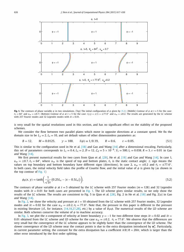
Fig. 1. The contours of phase variable φ in two simulations. (Top) The initial configuration of φ given by (5.2); (Middle) Contour of φ at t = 5 for the case: θs = 64◦ and uw = ±0.7; (Bottom) Contour of φ at t = 5 for the case: θs(y = ±1) = ±77.6◦ and uw = ±0.2. The results are generated by the LC scheme with 257 Fourier modes and 32 Legendre modes with δt = 0.01.

is very small for the spatial resolutions used in this section, and has no significant effect on the stability of the proposed schemes.

We consider the flow between two parallel plates which move in opposite directions at a constant speed. We fix the domain size to be L y = 2, Lx = 10, and set default values of other dimensionless parameters as:

B = 12, M = 0.0125, γ = 100, l(φ) ≡ 1/0.19, R = 0.6, ε = 0.05. (5.1)

This is similar to the configuration used in He et al. [18] and Gao and Wang [14] after a dimensional rescaling. Particularly, this set of parameters corresponds to Lz = 0.4, Lx = 2, B = 12, Ld = 5 × 10−4, Vs = 500, ls = 0.038, R = 3, ε = 0.01 in Gao and Wang [14].

We first present numerical results for two cases from Qian et al. [28], He et al. [18] and Gao and Wang [14]. In case 1, uw = ±0.7, θs = 64◦ , where uw is the speed of top and bottom plates, θs is the static contact angle; ± sign means the values on top boundary and bottom boundary have different signs (directions). In case 2, uw = ±0.2 and θs = ±77.6◦ . In both cases, the initial velocity field takes the profile of Couette flow, and the initial value of φ is given by (as shown in the top contour of Fig. 1)

φ0(x, y) = tanh

(1√2ε

(0.25Lx − |x − 0.5Lx|

)). (5.2)

The contours of phase variable φ at t = 5 obtained by the LC scheme with 257 Fourier modes (m = 128) and 32 Legendre modes with δt = 0.01 for both cases are presented in Fig. 1. The LD scheme gives similar results, so we only show the results of the LC scheme. The results are consistent to Fig. 5 in Qian et al. [28], Fig. 2 in He et al. [18] and Fig. 2(a) in Gao and Wang [14].

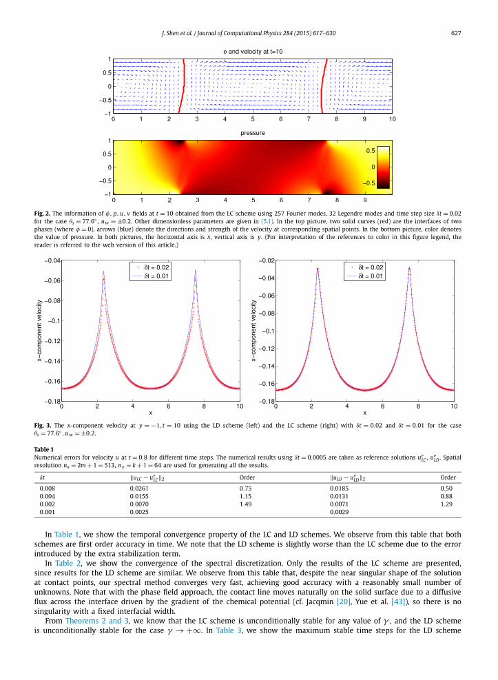
In Fig. 2, we show the velocity and pressure at t = 10 obtained from the LC scheme with 257 Fourier modes, 32 Legendre modes and δt = 0.02 for the case uw = ±0.2, θs = 77.6◦ . Note that, the pressure in this paper is different to the pressure in existing literature (cf., for instance, [14,18,27,28], etc.) by a value of Bμφ. The numerical results of the LD scheme are similar. Both schemes conserve the volume of φ to machine accuracy.

In Fig. 3, we plot the x-component of velocity at lower boundary y = −1 for two different time steps δt = 0.02 and δt =0.01 obtained from the LC scheme and LD scheme for the case uw = ±0.2, θs = 77.6◦ . We observe that the differences are very small but the convergence of the LC scheme appears to be slightly faster than the convergence of the LD scheme. The slower convergence of the LD scheme near the contact points is due to the extra dissipation introduced by un∗ . Particularly, in current parameter setting, the constant for the extra dissipation has a coefficient δt B/R = 20δt , which is larger than the other error introduced by the first order splitting.

J. Shen et al. / Journal of Computational Physics 284 (2015) 617–630 627

Fig. 2. The information of φ, p, u, v fields at t = 10 obtained from the LC scheme using 257 Fourier modes, 32 Legendre modes and time step size δt = 0.02for the case θs = 77.6◦ , uw = ±0.2. Other dimensionless parameters are given in (5.1). In the top picture, two solid curves (red) are the interfaces of two phases (where φ = 0), arrows (blue) denote the directions and strength of the velocity at corresponding spatial points. In the bottom picture, color denotes the value of pressure. In both pictures, the horizontal axis is x, vertical axis is y. (For interpretation of the references to color in this figure legend, the reader is referred to the web version of this article.)

Fig. 3. The x-component velocity at y = −1, t = 10 using the LD scheme (left) and the LC scheme (right) with δt = 0.02 and δt = 0.01 for the case θs = 77.6◦, uw = ±0.2.

Table 1Numerical errors for velocity u at t = 0.8 for different time steps. The numerical results using δt = 0.0005 are taken as reference solutions ue

LC , ueLD . Spatial

resolution nx = 2m + 1 = 513, ny = k + 1 = 64 are used for generating all the results.

δt ‖uLC − ueLC‖2 Order ‖uLD − ue

LD‖2 Order

0.008 0.0261 0.75 0.0185 0.500.004 0.0155 1.15 0.0131 0.880.002 0.0070 1.49 0.0071 1.290.001 0.0025 0.0029

In Table 1, we show the temporal convergence property of the LC and LD schemes. We observe from this table that both schemes are first order accuracy in time. We note that the LD scheme is slightly worse than the LC scheme due to the error introduced by the extra stabilization term.

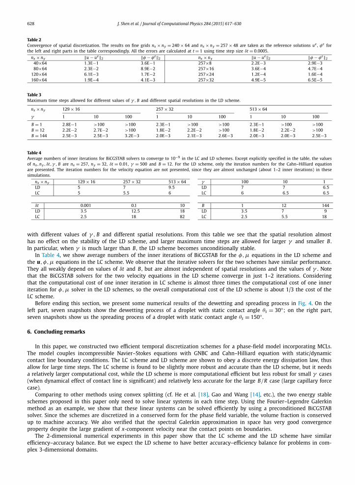
In Table 2, we show the convergence of the spectral discretization. Only the results of the LC scheme are presented, since results for the LD scheme are similar. We observe from this table that, despite the near singular shape of the solution at contact points, our spectral method converges very fast, achieving good accuracy with a reasonably small number of unknowns. Note that with the phase field approach, the contact line moves naturally on the solid surface due to a diffusive flux across the interface driven by the gradient of the chemical potential (cf. Jacqmin [20], Yue et al. [43]), so there is no singularity with a fixed interfacial width.

From Theorems 2 and 3, we know that the LC scheme is unconditionally stable for any value of γ , and the LD scheme is unconditionally stable for the case γ → +∞. In Table 3, we show the maximum stable time steps for the LD scheme

628 J. Shen et al. / Journal of Computational Physics 284 (2015) 617–630

Table 2Convergence of spatial discretization. The results on fine grids nx × ny = 240 × 64 and nx × ny = 257 × 48 are taken as the reference solutions ue , φe for the left and right parts in the table correspondingly. All the errors are calculated at t = 1 using time step size δt = 0.0005.

nx × ny ‖u − ue‖2 ‖φ − φe‖2 nx × ny ‖u − ue‖2 ‖φ − φe‖2

40×64 1.3E−1 3.6E−1 257×8 2.2E−3 2.9E−380×64 2.3E−2 8.9E−2 257×16 3.6E−4 4.7E−4

120×64 6.1E−3 1.7E−2 257×24 1.2E−4 1.6E−4160×64 1.9E−4 4.1E−3 257×32 4.9E−5 6.5E−5

Table 3Maximum time steps allowed for different values of γ , B and different spatial resolutions in the LD scheme.

nx × ny 129 × 16 257 × 32 513 × 64

γ 1 10 100 1 10 100 1 10 100

B = 1 2.8E−1 >100 >100 2.3E−1 >100 >100 2.3E−1 >100 >100B = 12 2.2E−2 2.7E−2 >100 1.8E−2 2.2E−2 >100 1.8E−2 2.2E−2 >100B = 144 2.5E−3 2.5E−3 3.2E−3 2.0E−3 2.1E−3 2.6E−3 2.0E−3 2.0E−3 2.5E−3

Table 4Average numbers of inner iterations for BiCGSTAB solvers to converge to 10−9 in the LC and LD schemes. Except explicitly specified in the table, the values of nx, ny , δt, γ , B are nx = 257, ny = 32, δt = 0.01, γ = 500 and B = 12. For the LD scheme, only the iteration numbers for the Cahn–Hilliard equation are presented. The iteration numbers for the velocity equation are not presented, since they are almost unchanged (about 1–2 inner iterations) in these simulations.

nx × ny 129 × 16 257 × 32 513 × 64LD 5 7 9.5LC 5 5.5 6

γ 100 10 1LD 7 7 6.5LC 6 6.5 6.5

δt 0.001 0.1 10LD 3.5 12.5 18LC 2.5 18 82

B 1 12 144LD 3.5 7 9LC 2.5 5.5 18

with different values of γ , B and different spatial resolutions. From this table we see that the spatial resolution almost has no effect on the stability of the LD scheme, and larger maximum time steps are allowed for larger γ and smaller B . In particular, when γ is much larger than B , the LD scheme becomes unconditionally stable.

In Table 4, we show average numbers of the inner iterations of BiCGSTAB for the φ, μ equations in the LD scheme and the u, φ, μ equations in the LC scheme. We observe that the iterative solvers for the two schemes have similar performance. They all weakly depend on values of δt and B , but are almost independent of spatial resolutions and the values of γ . Note that the BiCGSTAB solvers for the two velocity equations in the LD scheme converge in just 1–2 iterations. Considering that the computational cost of one inner iteration in LC scheme is almost three times the computational cost of one inner iteration for φ, μ solver in the LD schemes, so the overall computational cost of the LD scheme is about 1/3 the cost of the LC scheme.

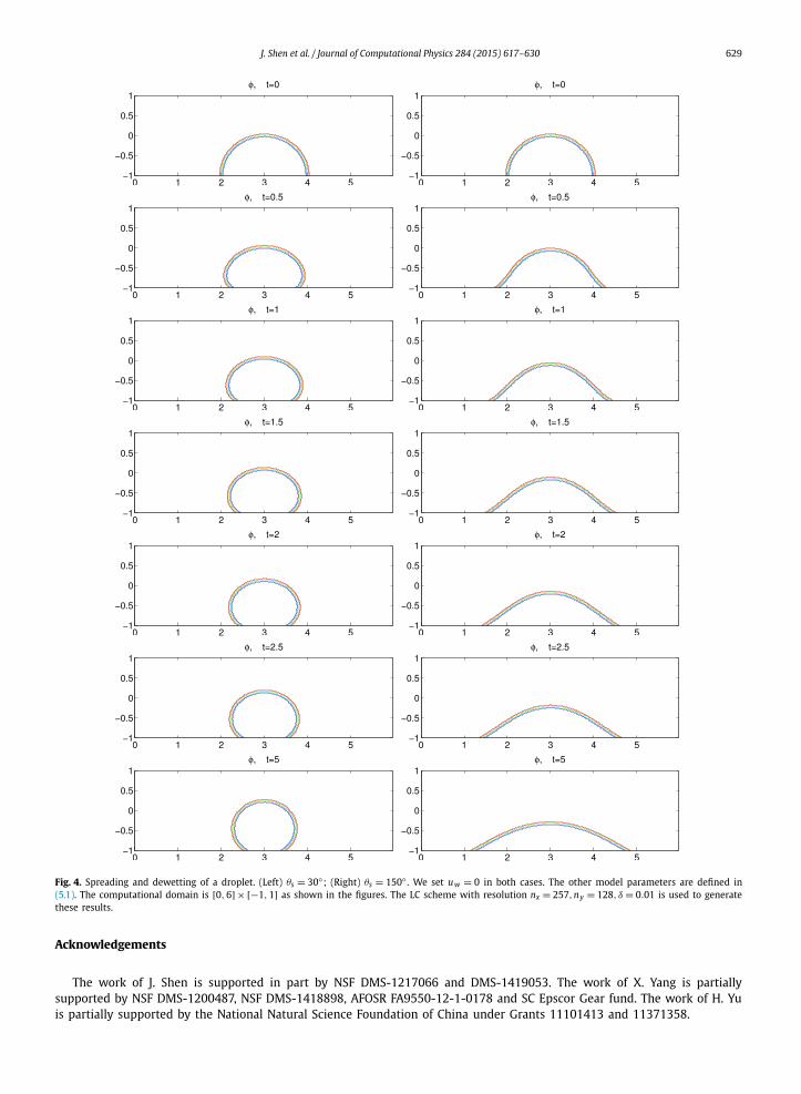
Before ending this section, we present some numerical results of the dewetting and spreading process in Fig. 4. On the left part, seven snapshots show the dewetting process of a droplet with static contact angle θs = 30◦; on the right part, seven snapshots show us the spreading process of a droplet with static contact angle θs = 150◦ .

6. Concluding remarks

In this paper, we constructed two efficient temporal discretization schemes for a phase-field model incorporating MCLs. The model couples incompressible Navier–Stokes equations with GNBC and Cahn–Hilliard equation with static/dynamic contact line boundary conditions. The LC scheme and LD scheme are shown to obey a discrete energy dissipation law, thus allow for large time steps. The LC scheme is found to be slightly more robust and accurate than the LD scheme, but it needs a relatively larger computational cost, while the LD scheme is more computational efficient but less robust for small γ cases (when dynamical effect of contact line is significant) and relatively less accurate for the large B/R case (large capillary force case).

Comparing to other methods using convex splitting (cf. He et al. [18], Gao and Wang [14], etc.), the two energy stable schemes proposed in this paper only need to solve linear systems in each time step. Using the Fourier–Legendre Galerkin method as an example, we show that these linear systems can be solved efficiently by using a preconditioned BiCGSTAB solver. Since the schemes are discretized in a conserved form for the phase field variable, the volume fraction is conserved up to machine accuracy. We also verified that the spectral Galerkin approximation in space has very good convergence property despite the large gradient of x-component velocity near the contact points on boundaries.

The 2-dimensional numerical experiments in this paper show that the LC scheme and the LD scheme have similar efficiency–accuracy balance. But we expect the LD scheme to have better accuracy–efficiency balance for problems in com-plex 3-dimensional domains.

J. Shen et al. / Journal of Computational Physics 284 (2015) 617–630 629

Fig. 4. Spreading and dewetting of a droplet. (Left) θs = 30◦; (Right) θs = 150◦ . We set uw = 0 in both cases. The other model parameters are defined in (5.1). The computational domain is [0, 6] × [−1, 1] as shown in the figures. The LC scheme with resolution nx = 257, ny = 128, δ = 0.01 is used to generate these results.

Acknowledgements

The work of J. Shen is supported in part by NSF DMS-1217066 and DMS-1419053. The work of X. Yang is partially supported by NSF DMS-1200487, NSF DMS-1418898, AFOSR FA9550-12-1-0178 and SC Epscor Gear fund. The work of H. Yu is partially supported by the National Natural Science Foundation of China under Grants 11101413 and 11371358.

630 J. Shen et al. / Journal of Computational Physics 284 (2015) 617–630

References

[1] S. Aland, F. Chen, An efficient and energy stable scheme for a phase-field model for the moving contact line problem, preprint, 2014.[2] A. Bray, Theory of phase-ordering kinetics, Adv. Phys. 43 (3) (1994) 357–459.[3] L.A. Caffarelli, N.E. Muler, An L∞ bound for solutions of the Cahn–Hilliard equation, Arch. Ration. Mech. Anal. 133 (2) (Dec. 1995) 129–144.[4] J.W. Cahn, J.E. Hilliard, Free energy of a nonuniform system. I. Interfacial free energy, J. Chem. Phys. 28 (2) (Feb. 1958) 258–267.[5] N. Condette, C. Melcher, E. Süli, Spectral approximation of pattern-forming nonlinear evolution equations with double-well potentials of quadratic

growth, Math. Comput. 80 (273) (2011) 205–223.[6] S. Dong, On imposing dynamic contact-angle boundary conditions for wall-bounded liquid–gas flows, Comput. Methods Appl. Mech. Eng. 247–248

(Nov. 2012) 179–200.[7] S. Dong, J. Shen, A time-stepping scheme involving constant coefficient matrices for phase-field simulations of two-phase incompressible flows with

large density ratios, J. Comput. Phys. 231 (17) (2012) 5788–5804.[8] Q. Du, R.A. Nicolaides, Numerical analysis of a continuum model of phase transition, SIAM J. Numer. Anal. 28 (5) (1991) 1310–1322.[9] E.B. Dussan V., On the spreading of liquids on solid surfaces: static and dynamic contact lines, Annu. Rev. Fluid Mech. 11 (1) (1979) 371–400.

[10] E.B. Dussan V., S.H. Davis, On the motion of a fluid–fluid interface along a solid surface, J. Fluid Mech. 65 (01) (1974) 71–95.[11] C.M. Elliott, A.M. Stuart, The global dynamics of discrete semilinear parabolic equations, SIAM J. Numer. Anal. 30 (1993) 1622–1663.[12] D.J. Eyre, Unconditionally gradient stable time marching the Cahn–Hilliard equation, MRS Proc. 529 (1998).[13] D. Furihata, A stable and conservative finite difference scheme for the Cahn–Hilliard equation, Numer. Math. 87 (4) (Feb. 2001) 675–699.[14] M. Gao, X.-P. Wang, A gradient stable scheme for a phase field model for the moving contact line problem, J. Comput. Phys. 231 (4) (Feb. 2012)

1372–1386.[15] M. Gao, X.-P. Wang, An efficient scheme for a phase field model for the moving contact line problem with variable density and viscosity, J. Comput.

Phys. 272 (2014) 704–718.[16] J. Guermond, P. Minev, J. Shen, An overview of projection methods for incompressible flows, Comput. Methods Appl. Mech. Eng. 195 (44–47) (Sep.

2006) 6011–6045.[17] N.G. Hadjiconstantinou, Hybrid atomistic–continuum formulations and the moving contact-line problem, J. Comput. Phys. 154 (2) (Sep. 1999) 245–265.[18] Q. He, R. Glowinski, X.-P. Wang, A least-squares/finite element method for the numerical solution of the Navier–Stokes–Cahn–Hilliard system modeling

the motion of the contact line, J. Comput. Phys. 230 (12) (Jun. 2011) 4991–5009.[19] Y. He, Y. Liu, T. Tang, On large time-stepping methods for the Cahn–Hilliard equation, Appl. Numer. Math. 57 (5–7) (May 2007) 616–628.[20] D. Jacqmin, Contact-line dynamics of a diffuse fluid interface, J. Fluid Mech. 402 (2000) 57–88.[21] D. Kessler, R.H. Nochetto, A. Schmidt, A posteriori error control for the Allen–Cahn problem: circumventing Gronwall’s inequality, ESAIM: Math. Model.

Numer. Anal. 38 (01) (2004) 129–142.[22] J. Koplik, J.R. Banavar, J.F. Willemsen, Molecular dynamics of Poiseuille flow and moving contact lines, Phys. Rev. Lett. 60 (13) (Mar. 1988) 1282–1285.[23] J. Koplik, J.R. Banavar, J.F. Willemsen, Molecular dynamics of fluid flow at solid surfaces, Phys. Fluids A, Fluid Dyn. 1 (5) (May 1989) 781–794.[24] C. Liu, J. Shen, A phase field model for the mixture of two incompressible fluids and its approximation by a Fourier-spectral method, Physica D:

Nonlinear Phenom. 179 (3–4) (May 2003) 211–228.[25] S. Minjeaud, An unconditionally stable uncoupled scheme for a triphasic Cahn–Hilliard/Navier–Stokes model, Numer. Methods Partial Differ. Equ. 29 (2)

(Mar. 2013) 584–618.[26] H.K. Moffatt, Viscous and resistive Eddies near a Sharp corner, J. Fluid Mech. 18 (01) (1964) 1–18.[27] T. Qian, X.-P. Wang, P. Sheng, Molecular scale contact line hydrodynamics of immiscible flows, Phys. Rev. E 68 (1) (2003) 016306.[28] T. Qian, X.-P. Wang, P. Sheng, A variational approach to moving contact line hydrodynamics, J. Fluid Mech. 564 (2006) 333–360.[29] L. Rayleigh, XX. On the theory of surface forces II. Compressible fluids, Philos. Mag. Ser. 5 33 (201) (Feb. 1892) 209–220.[30] W. Ren, W. E, Heterogeneous multiscale method for the modeling of complex fluids and micro-fluidics, J. Comput. Phys. 204 (1) (Mar. 2005) 1–26.[31] A.J. Salgado, A diffuse interface fractional time-stepping technique for incompressible two-phase flows with moving contact lines, ESAIM: Math. Model.

Numer. Anal. 47 (3) (May 2013) 743–769.[32] J. Shen, Efficient spectral-Galerkin method I. Direct solvers of second- and fourth-order equations using Legendre polynomials, SIAM J. Sci. Comput.

15 (6) (1994) 1489.[33] J. Shen, Modeling and numerical approximation of two-phase incompressible flows by a phase-field approach, in: W. Bao, Q. Du (Eds.), Multiscale

Modeling and Analysis for Materials Simulation, in: Lecture Note Series, vol. 9, IMS, National University of Singapore, 2011, pp. 147–196.[34] J. Shen, X. Yang, Energy stable schemes for Cahn–Hilliard phase-field model of two-phase incompressible flows, Chin. Ann. Math., Ser. B 31 (5) (Sep.

2010) 743–758.[35] J. Shen, X. Yang, Numerical approximations of Allen–Cahn and Cahn–Hilliard equations, Discrete Contin. Dyn. Syst., Ser. A 28 (2010) 1669–1691.[36] J. Shen, X. Yang, A phase-field model and its numerical approximation for two-phase incompressible flows with different densities and viscosities,

SIAM J. Sci. Comput. 32 (3) (2010) 1159–1179.[37] J. Shen, X. Yang, Decoupled energy stable schemes for phase-field models of two-phase complex fluids, SIAM J. Sci. Comput. 36 (1) (2014) B122–B145.[38] J. Shen, X. Yang, Decoupled, energy stable schemes for phase-field models of two-phase incompressible flows, SIAM J. Numer. Anal. (2015), in press.[39] P.A. Thompson, M.O. Robbins, Simulations of contact-line motion: slip and the dynamic contact angle, Phys. Rev. Lett. 63 (7) (Aug. 1989) 766–769.[40] H. van der Vorst, Bi-CGSTAB: a fast and smoothly converging variant of bi-CG for the solution of nonsymmetric linear systems, SIAM J. Sci. Stat.

Comput. 13 (2) (1992) 631–644.[41] J.D. van der Waals, The thermodynamic theory of capillarity under the hypothesis of a continuous variation of density, J. Stat. Phys. 20 (2) (Feb. 1893)

200–244, Transl. by J.S. Rowlinson.[42] C. Xu, T. Tang, Stability analysis of large time-stepping methods for epitaxial growth models, Liq. Cryst. 44 (2006) 1759–1779.[43] P. Yue, C. Zhou, J.J. Feng, Sharp-interface limit of the Cahn–Hilliard model for moving contact lines, J. Fluid Mech. 645 (2010) 279–294.[44] J. Zhu, L.-Q. Chen, J. Shen, V. Tikare, Coarsening kinetics from a variable-mobility Cahn–Hilliard equation: application of a semi-implicit Fourier spectral

method, Phys. Rev. E 60 (4) (Oct. 1999) 3564–3572.