Journal of Computational Physics 273 (2014) 416–434

Contents lists available at ScienceDirect

Journal of Computational Physics

www.elsevier.com/locate/jcp

A fast pressure-correction method for incompressible

two-fluid flows

Michael S. Dodd 1, Antonino Ferrante ∗,2

William E. Boeing Department of Aeronautics & Astronautics, University of Washington, Seattle, WA 98195, USA

a r t i c l e i n f o a b s t r a c t

Article history:Received 17 October 2013Received in revised form 7 March 2014Accepted 19 May 2014Available online 28 May 2014

Keywords:Variable density Navier–Stokes equationsProjection methodVolume-of-fluid methodMultiphase flowInterfacial flowTurbulent flowDirect numerical simulation

We have developed a new pressure-correction method for simulating incompressible two-fluid flows with large density and viscosity ratios. The method’s main advantage is that the variable coefficient Poisson equation that arises in solving the incompressible Navier–Stokes equations for two-fluid flows is reduced to a constant coefficient equation, which can be solved with an FFT-based, fast Poisson solver. This reduction is achieved by splitting the variable density pressure gradient term in the governing equations. The validity of this splitting is demonstrated from our numerical tests, and it is explained from a physical viewpoint.In this paper, the new pressure-correction method is coupled with a mass-conserving volume-of-fluid method to capture the motion of the interface between the two fluids but, in general, it could be coupled with other interface advection methods such as level-set, phase-field, or front-tracking. First, we verified the new pressure-correction method using the capillary wave test-case up to density and viscosity ratios of 10,000. Then, we validated the method by simulating the motion of a falling water droplet in air and comparing the droplet terminal velocity with an experimental value. Next, the method is shown to be second-order accurate in space and time independent of the VoF method, and it conserves mass, momentum, and kinetic energy in the inviscid limit. Also, we show that for solving the two-fluid Navier–Stokes equations, the method is 10–40 times faster than the standard pressure-correction method, which uses multigrid to solve the variable coefficient Poisson equation. Finally, we show that the method is capable of performing fully-resolved direct numerical simulation (DNS) of droplet-laden isotropic turbulence with thousands of droplets using a computational mesh of 10243 points.

© 2014 Elsevier Inc. All rights reserved.

1. Introduction

In the incompressible flow of two immiscible fluids, the density is discontinuous at the interface, and the density ratio can be of order one thousand (e.g., air–water). Thus, simulating two-fluid flows using a constant density approximation, e.g., the Boussinesq approximation, is not justified. Therefore, the density change between the two fluids must be accounted for directly when solving the governing equations of fluid motion. From a numerical point of view, this introduces additional

* Corresponding author.E-mail addresses: doddms@uw.edu (M.S. Dodd), ferrante@aa.washington.edu (A. Ferrante).

1 Ph.D. candidate, William E. Boeing Department of Aeronautics & Astronautics, University of Washington, Seattle.2 Assistant Professor, William E. Boeing Department of Aeronautics & Astronautics, University of Washington, Seattle.

http://dx.doi.org/10.1016/j.jcp.2014.05.0240021-9991/© 2014 Elsevier Inc. All rights reserved.

M.S. Dodd, A. Ferrante / Journal of Computational Physics 273 (2014) 416–434 417

challenges which are not present when solving incompressible single-fluid flows. These challenges are to obtain a numerical method that is computationally efficient, second-order accurate, and stable for large density ratios.

A common solution technique for the incompressible Navier–Stokes equations is the projection method [1]. In the pro-jection method, a Poisson equation for pressure must be solved numerically at each time step. This operation takes most of the computational time in the projection method. Consequently, much work has gone into developing so-called “fast Pois-son solvers”, which use a combination of fast Fourier transforms (FFT) and Gauss elimination to solve the Poisson equation directly in Fourier space (e.g., [2–5]). However, fast Poisson solvers cannot solve the Poisson equation for pressure that arises in two-fluid flows when advancing the solution from time tn to tn+1 (�t = tn+1 − tn):

∇ ·(

1

ρn+1∇pn+1

)= 1

�t∇ · u∗, Al (1)

where ρ is the density, p is the pressure, and u∗ is the approximate velocity field at tn+1. Fast Poisson solvers require a constant coefficient on the left-hand side of the Poisson equation, whereas the coefficient (1/ρn+1) on the left-hand side of Eq. (1) varies in space and time. To solve the variable coefficient equation (1), a standard practice has been to use iterative methods, e.g., multigrid methods [6–8], Krylov methods [9,10] or Krylov methods preconditioned with multigrid [11]. The downside is that iterative methods are often slower than fast Poisson solvers. In fact, they can be up to ten times slower [2]. Additionally, an iterative method’s operation count depends on problem parameters (e.g., density ratio) and convergence tolerance, whereas fast Poisson solvers have the advantage of fixed operation counts.

To reduce the computational time in solving variable density incompressible flows, Guermond and Salgado [12] adopted a penalty formulation, whereby only a constant coefficient Poisson equation must be solved at each time step. More recently, for solving the two-fluid coupled Navier–Stokes Cahn–Hilliard (phase-field) equations, Dong and Shen [13] developed a velocity-correction method that transforms the Poisson equation (1) from a variable to a constant coefficient equation. The underlying idea is to split the variable-coefficient pressure-gradient term into a constant term and a variable term, and then treat the constant term implicitly and the variable term explicitly as

1

ρn+1∇pn+1 → 1

ρ0∇pn+1 +

(1

ρn+1− 1

ρ0

)∇ p, (2)

where ρ0 is a constant to be defined in Section 2 and p is an explicit approximation to the pressure at time level n + 1, specifically,

p ={

pn if J = 1,

p∗ = 2pn − pn−1 if J = 2,(3)

where the choice of J = 1 or 2 indicates, respectively, constant or linear extrapolation of pn+1.3 Then, applying the substi-tution (Eq. (2)) to the left-hand side of Eq. (1), leads to a constant coefficient Poisson equation for pressure,

∇2 pn+1 = ∇ ·[(

1 − ρ0

ρn+1

)∇ p

]+ ρ0

�t∇ · u∗ (4)

that can be solved directly using a fast Poisson solver. Also, in contrast to solving Eq. (1), there is no need to assemble variable coefficient matrices at each time step when solving Eq. (4). Therefore, by using the splitting technique in Eq. (2), there is potential for significant speedup in solving the Navier–Stokes equations for incompressible two-fluid flows.

In this paper, we aim to answer the following questions on applying the splitting technique (Eq. (2)) to the two-fluid Navier–Stokes equations:

• Is the split method (Eq. (4)) physically less accurate than the unsplit method (Eq. (1)) and does the accuracy of the split method depend on the type of extrapolation chosen in Eq. (3)?

• What are the computational savings of using the split method? Specifically, how much faster is it to solve Eq. (4)directly versus Eq. (1) iteratively?

To answer these questions, we first develop a two-fluid pressure-correction method with a constant coefficient Poisson equation, which can be solved directly with a fast Poisson solver. Next, we apply the method to several two-fluid flows to verify and validate the new method, quantify its performance, and evaluate its spatial and temporal accuracy.

The paper is organized as follows: in Section 2 we describe the new pressure-correction method for uniform Cartesian grids and periodic boundary conditions and its coupling to the volume-of-fluid (VoF) method. Section 3 compares the numerical solutions obtained when using the standard, unsplit method (i.e., solving Eq. (1), called Unsplit), the split method, Eq. (2), using J = 1 (called FastPn), and the split method using J = 2 (called FastP∗). Next, we assess the performance of the unsplit and split formulations by comparing the CPU time when solving Eq. (1) using a multigrid solver to the CPU time

3 A similar strategy for handling variable coefficients in the advection–diffusion equation was proposed by Gottlieb and Orszag [14, Section 9, p. 114].

418 M.S. Dodd, A. Ferrante / Journal of Computational Physics 273 (2014) 416–434

when solving Eq. (4) using a fast Poisson solver. Section 4 verifies and validates the new pressure-correction/volume-of-fluid flow solver. This includes two canonical flows and DNS of droplet-laden decaying isotropic turbulence.

The potential computational savings suggest that our method is well-suited for fully-resolved DNS of bubble- and droplet-laden turbulent flows in simple geometries. In addition, because Eq. (1) is present regardless of the method used to advect the fluid interface, the pressure-correction method presented is useful in other interface-capturing (e.g., level-set or phase-field) and front-tracking methods. Furthermore, the splitting technique of the new pressure-correction method could be extended to simulate low-Mach number flows that use the pressure-correction method, e.g., [15].

2. Mathematical description

2.1. Governing equations

The governing equations for the incompressible flow of two immiscible fluids are

∇ · u = 0, (5a)

∂u

∂t+ ∇ · (uu) = 1

ρ

[−∇p + 1

Re∇ ·

(μ

(∇u + ∇uT )) + 1

Wefσ

]+ 1

Frg (5b)

where u = u(x, t) is the fluid velocity, p = p(x, t) is the pressure, ρ = ρ(x, t) is the density, μ = μ(x, t) is the dynamic viscosity, g is the gravitational acceleration, and fσ = fσ (x, t) is the force per unit volume due to surface tension,

fσ = σκδ(x − xs)n, (6)

where σ is the surface tension coefficient, κ is the curvature of the interface between the two fluids (denoted fluid 1 and fluid 2), n is the unit normal pointing into fluid 2 at the interface, and δ is the Dirac δ-function that is needed to impose the force only at the interface position xs . In this paper, the surface tension coefficient is constant in space and time, and the symbol σ is replaced by its non-dimensional value 1/We. In Eq. (5b), Re, We, and Fr are, respectively, the Reynolds, Weber, and Froude numbers defined as:

Re = U Lρ1

μ1, We = ρ1U 2 L

σ, Fr = U 2

g L, (7)

where U , L, ρ1, μ1, σ , and g denote, in order, the reference dimensional velocity, length, density, dynamic viscosity, surface tension coefficient, and gravitational acceleration used to non-dimensionalize the governing equations (5a) and (5b). The subscripts 1 and 2 indicate fluid 1 and fluid 2, respectively. We have chosen to non-dimensionalize the density and dynamic viscosity in Eq. (5b) by choosing fluid 1 as the reference phase, which makes ρ1 = 1 and μ1 = 1. Throughout the paper, all variables are dimensionless unless they are accented with ∼. Also, we impose periodic boundary conditions in all spatial directions unless noted otherwise.

2.2. Pressure-correction method

Our two-fluid pressure-correction method is developed starting from that of Chorin [1] and Temam [16] for single-phase flows. The solution algorithm proceeds by advecting the volume fraction of fluid 2, C(x, t), based on the known velocity field un . The VoF advection algorithm [17] that computes Cn+1(x) is briefly described in the next section. The volume fraction has value C = 0 in fluid 1, C = 1 in fluid 2, and 0 < C < 1 in cells containing the interface separating the two fluids. After computing Cn+1, the density and viscosity are computed at time level n + 1 as

ρn+1(x) = ρ2Cn+1(x) + ρ1[1 − Cn+1(x)

]μn+1(x) = μ2Cn+1(x) + μ1

[1 − Cn+1(x)

]. (8)

Next, an approximate velocity is computed by first defining RUn as

RUn = −∇ · (unun) + 1

Re

[1

ρn+1∇ · (μn+1(∇un + (∇un)T ))] + 1

We

[1

ρn+1κn+1∇Cn+1

]+ 1

Frg, (9)

which is the right-hand side of the momentum equation (5b) without the pressure gradient term. The surface tension force, fσ , is computed as fσ = σκ∇C by adopting Brackbill’s continuum surface force approach [18]. Next, as recommended in [18], we multiply fσ in Eq. (5b) by ρ(x, t)/〈ρ〉, where 〈ρ〉 ≡ 1

2 (ρ1 +ρ2), such that fσ is constant across the interface, which reduces the magnitude of the spurious currents at high density ratios (not shown). Thus, Eq. (9) becomes

RUn = −∇ · (unun) + 1

Re

[1

ρn+1∇ · (μn+1(∇un + (∇un)T ))] + 1

We

[κn+1∇Cn+1

〈ρ〉]

+ 1

Frg. (10)

The interface curvature κn+1 is computed using the height-function method [19] with improvements by López et al. [20]. The equations are integrated in time using the Adams–Bashforth scheme:

M.S. Dodd, A. Ferrante / Journal of Computational Physics 273 (2014) 416–434 419

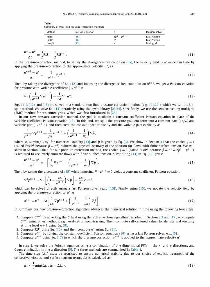
Table 1Summary of two-fluid pressure-correction methods.

Method Poisson equation p Poisson solver

FastP∗ (16) 2pn − pn−1 Fast PoissonFastPn (16) pn Fast PoissonUnsplit (13) – Multigrid

u∗ − un

�t= 3

2RUn − 1

2RUn−1. (11)

In the pressure-correction method, to satisfy the divergence-free condition (5a), the velocity field is advanced in time by applying the pressure-correction to the approximate velocity, u∗ , as

un+1 − u∗

�t= − 1

ρn+1∇pn+1. (12)

Then, by taking the divergence of Eq. (12) and imposing the divergence-free condition on un+1, we get a Poisson equation for pressure with variable coefficient (1/ρn+1):

∇ ·(

1

ρn+1∇pn+1

)= 1

�t∇ · u∗. (13)

Eqs. (11), (12), and (13) are solved in a standard, two-fluid pressure-correction method (e.g., [21,22]), which we call the Un-split method. We solve Eq. (13) iteratively using the hypre library [23,24]. Specifically, we use the semicoarsening multigrid (SMG) method for structured grids, which was first introduced in [25].

In our new pressure-correction method, the goal is to obtain a constant coefficient Poisson equation in place of the variable coefficient Poisson equation (13). To this end, we split the pressure gradient term into a constant part (1/ρ0) and variable part (1/ρn+1), and then treat the constant part implicitly and the variable part explicitly as

1

ρn+1∇pn+1 → 1

ρ0∇pn+1 +

(1

ρn+1− 1

ρ0

)∇ p, (14)

where ρ0 = min(ρ1, ρ2) for numerical stability [13] and p is given by Eq. (3). We show in Section 3 that the choice J = 1(called FastPn because p = pn) reduces the physical accuracy of the solution for flows with finite surface tension. We will show in Section 3 that, for our pressure-correction method, the choice J = 2 (called FastP∗ because p = p∗ = 2pn − pn−1), is required to accurately simulate flows with finite surface tension. Substituting (14) in Eq. (12) gives:

un+1 − u∗

�t= −

[1

ρ0∇pn+1 +

(1

ρn+1− 1

ρ0

)∇ p

]. (15)

Then, by taking the divergence of (15) while imposing ∇ · un+1 = 0 yields a constant coefficient Poisson equation,

∇2 pn+1 = ∇ ·[(

1 − ρ0

ρn+1

)∇ p

]+ ρ0

�t∇ · u∗, (16)

which can be solved directly using a fast Poisson solver (e.g., [4,5]). Finally, using (15), we update the velocity field by applying the pressure-correction to u∗ as

un+1 = u∗ − �t

[1

ρ0∇pn+1 +

(1

ρn+1− 1

ρ0

)∇ p

]. (17)

In summary, our new pressure-correction algorithm advances the numerical solution in time using the following four steps:

1. Compute Cn+1 by advecting the C field using the VoF advection algorithm described in Section 2.3 and [17], or compute Cn+1 using other methods, e.g., level-set or front-tracking. Then, compute cell-centered values for density and viscosity at time level n + 1 using Eq. (8).

2. Compute RUn using Eq. (10), and then compute u∗ using Eq. (11).3. Compute pn+1 by solving the constant-coefficient Poisson equation (16) using a fast Poisson solver, e.g., [5].4. Compute un+1 using Eq. (17) in which the pressure correction pn+1 is applied to the approximate velocity u∗ .

In step 3, we solve the Poisson equation using a combination of one-dimensional FFTs in the x- and y-directions, and Gauss elimination in the z-direction [5]. The three methods are summarized in Table 1.

The time step (�t) must be restricted to ensure numerical stability due to our choice of explicit treatment of the convective, viscous, and surface tension terms. �t is calculated as

�t ≤ 1min(�tc,�tν,�tσ ), (18)

2

420 M.S. Dodd, A. Ferrante / Journal of Computational Physics 273 (2014) 416–434

where

�tc = �x

|U |max(19)

�tν = Re �x2

6(20)

�tσ =√

We(ρ1 + ρ2)�x3

4π. (21)

For cases of low Re, the viscous stability restriction (20) can be eliminated by treating the viscous terms implicitly (see Appendix A), however, in all the simulations presented in this paper, the viscous terms were treated explicitly as in Eq. (10)either because: (i) �tν > �tσ , (ii) the stability restriction imposed by large density and viscosity gradients was greater than the restriction imposed by �tν , or (iii) switching to implicit time integration would not reduce the number of time steps enough to offset the additional computational cost of solving three Helmholtz equations at each time step. For cases of low We, the capillary time step restriction (21) can be lessened by a method outlined in [26] or eliminated by treating the surface tension implicitly [27], however these options were not pursued for this paper.

Finally, the numerical methods described in this section have been implemented using Fortran 90, the message passing interface (MPI), OpenMP, and FFTW [28]. To perform parallel multi-core simulations, the domain is decomposed such that the data is distributed in memory in the y-direction and contiguous in memory in the x- and z-directions. The following algorithm is used to solve the Poisson equation for pn+1 in parallel.

Algorithm of parallel fast Poisson solver (PFPS).

1. Perform real-to-complex FFT in the x-direction to the right-hand side of Eq. (16), which is a three-dimensional (3-D) scalar field;

2. Transpose the 3-D complex data among the computing cores such that the resulting data is distributed in the x-direction and contiguous in the y-direction;

3. Perform complex-to-complex FFT in the y-direction of the 3-D data;4. Perform Gauss elimination in the z-direction to obtain pn+1 in Fourier space [5];5. Perform complex-to-complex, inverse FFT in the y-direction of the 3-D data;6. Transpose the 3-D complex data among the computing cores such that it is distributed in the y-direction and contiguous

in the x-direction;7. Perform complex-to-real, inverse FFT in the x-direction of the resulting 3-D data to obtain pn+1.

2.2.1. Spatial discretizationWe discretize Eqs. (10), (16), and (17) in 3-D on a uniform staggered Cartesian mesh using central differences. For

brevity, we report here the details of the spatial discretization in 2-D. The extension to 3-D follows analogously from the 2-D discretization. The u-component of velocity is located at xi+1/2, j , the v-component at xi, j+1/2, and all other variables are centered at xi, j . Our discretization has the advantage over colocated schemes of not requiring an auxiliary cell-centered velocity field.

We begin discretizing Eq. (10) by categorizing the terms as convective fluxes RCU, diffusive fluxes RDU, and body forces RBU (surface tension and gravity):

RU = RCU + RDU + RBU (22)

with

RCU = −∇ · (unun)RDU = 1

Re

[1

ρn+1∇ · (μn+1(∇un + (∇un)T ))]

RBU = 1

We

[κn+1∇Cn+1

〈ρ〉]

+ 1

Frg. (23)

The convective fluxes RCU are equivalent to those found in one-fluid flow so we do not include their discretization here (see, e.g., [29]). We include the discretization of RDU and RBU for completeness and because there is no well-established second-order discretization of these terms. The components of the viscous flux vector RDU are discretized and computed as follows:

RDUi+1/2, j = 1

Re

1

(ρi+1/2, j)

(DUXi+1, j − DUXi, j

�x+ DUYi+1/2, j+1/2 − DUYi+1/2, j−1/2

�y

)(24)

and

M.S. Dodd, A. Ferrante / Journal of Computational Physics 273 (2014) 416–434 421

RDVi, j+1/2 = 1

Re

1

(ρi, j+1/2)

(DUYi+1/2, j+1/2 − DUYi+1/2, j−1/2

�x+ DVYi, j+1 − DVYi, j

�y

), (25)

where �x and �y are the grid sizes in the x- and y-directions, respectively. In Eqs. (24) and (25), the density at the staggered locations is computed using the arithmetic mean as

ρi+1/2, j = 1

2(ρi+1, j + ρi, j) and ρi, j+1/2 = 1

2(ρi, j+1 + ρi, j). (26)

The strain rates in Eqs. (24) and (25) are calculated as

DUXi, j = 2μi, j

(ui+1/2, j − ui−1/2, j

�x

)(27)

DUYi+1/2, j+1/2 = μi+1/2, j+1/2

(ui+1/2, j+1 − ui+1/2, j

�y+ vi+1, j+1/2 − vi, j+1/2

�x

)(28)

DVYi, j = 2μi, j

(vi, j+1/2 − vi, j−1/2

�y

), (29)

where the staggered viscosity in Eq. (28) is computed using the arithmetic mean

μi+1/2, j+1/2 = 1

4(μi+1, j+1 + μi+1, j + μi, j+1 + μi, j). (30)

Note that in Eq. (24), we substituted DUY for DVX because of the symmetry of the rate-of-strain tensor.Next, we compute the components of the body force vector RBU where the non-dimensional gravitational acceleration

in Eq. (5b) is g = 1 and in the negative y-direction (g = −j). Special treatment is required when gravity is oriented in the direction of periodic boundaries to prevent uniform acceleration of both fluids [7,30]. We explicitly account for the hydrostatic pressure term in the momentum equation (5b) by adding fh/ρ to the right-hand side of Eq. (5b), where

fh = −ρ1 V 1 + ρ2 V 2

V 1 + V 2g, (31)

and V 1 and V 2 are the total volumes of fluid 1 and 2. The discretized components of RBU are

RBUi+1/2, j = 1

We

κi+1/2, j

〈ρ〉(

Ci+1, j − Ci, j

�x

)(32)

RBVi, j+1/2 = 1

We

κi, j+1/2

〈ρ〉(

Ci, j+1 − Ci, j

�y

)+ 1

Fr

(fh

ρi, j+1/2− 1

), (33)

where, as a reminder, 〈ρ〉 ≡ 12 (ρ1 + ρ2).

The surface tension force fσ must be discretized at the staggered grid locations to be consistent with the location of the pressure gradient term [9]. This discretization produces an exact balance of the pressure gradient and the surface tension if the curvature is exact [17]. The curvature is computed at the staggered grid point xi+1/2, j as

κi+1/2, j =

⎧⎪⎨⎪⎩

κi+1, j if κi, j = 0

κi, j if κi+1, j = 012 (κi+1, j + κi, j) otherwise.

(34)

Next, we discretize the right-hand side of Eq. (16), which serves as input to the fast Poisson solver:

∇2 pn+1i, j = DPXi+1/2, j − DPXi−1/2, j

�x+ DPYi, j+1/2 − DPYi, j−1/2

�y+ DIVUi, j (35)

where

DPXi+1/2, j =(

1 − ρ0

ρi+1/2, j

)(pi+1, j − pi, j

�x

), (36)

DPYi, j+1/2 =(

1 − ρ0

ρi, j+1/2

)(pi, j+1 − pi, j

�y

), (37)

and

DIVUi, j = ρ0

�t

(u∗

i+1/2, j − u∗i−1/2, j

�x+ v∗

i, j+1/2 − v∗i, j−1/2

�y

). (38)

Finally, the components of Eq. (17) are discretized as

422 M.S. Dodd, A. Ferrante / Journal of Computational Physics 273 (2014) 416–434

un+1i+1/2, j = u∗

i+1/2, j − �t

[1

ρ0

(pn+1

i+1, j − pn+1i, j

�x

)+

(1

ρi+1/2, j− 1

ρ0

)(pi+1, j − pi, j

�x

)](39)

and

vn+1i, j+1/2 = v∗

i+1/2, j − �t

[1

ρ0

(pn+1

i, j+1 − pn+1i, j

�y

)+

(1

ρi, j+1/2− 1

ρ0

)(pi, j+1 − pi, j

�y

)]. (40)

2.3. Volume-of-fluid method

We are using a recently developed VoF method that is mass-conserving, consistent (0 ≤ C ≤ 1), and wisps-free [17]. A brief description is reported here.

In the VoF method, the sharp interface between the two immiscible fluids is determined using the VoF color function, C , which represents the volume fraction of fluid 2 in each computational cell. In our VoF method, the interface between the two phases is reconstructed using a piecewise linear interface calculation (PLIC) [31]. The interface reconstruction in each computational cell consists of two steps: the computation of the interface normal n = (nx, ny, nz) and the computation of the interface location. The algorithm that we use to evaluate the interface normal is a combination of the centered-columns method [32] and Youngs’ method [31] known as the mixed-Youngs-centered (MYC) method [33].

We define a characteristic function χ that has value χ = 1 in fluid 2 and χ = 0 in fluid 1. χ is governed by the following advection equation:

∂χ

∂t+ u · ∇χ = 0. (41)

The volume fraction Ci, j,k of grid cell i, j, k is related to the characteristic function χ by the integral relation

Ci, j,k(t) = 1

V 0

∫Ω

χ(x, t)dx, (42)

where V 0 is the volume of the i, j, k cell.The volume fraction C is advanced in time using the Eulerian implicit – Eulerian algebraic – Lagrangian explicit (EI-

EA-LE) algorithm originally proposed by Scardovelli et al. [34]. The original EI-EA-LE algorithm is globally mass-conserving but generates wisps and does not conserve the mass of the individual volumes tracked in the flow. We have improved this method by adding redistribution and wisp-suppression algorithms [17]. The redistribution algorithm corrects small in-consistencies in the volume fraction values (i.e., C < 0 and C > 1) that arise in the Eulerian algebraic (EA) step. The wisp suppression algorithm removes small errors arising from the finite machine precision. Because our method is consistent and wisps-free, it conserves mass both globally and locally within each fluid. The cell-centered volume fraction C is ad-vected using the face-centered velocity field. The method displays second-order spatial accuracy for values of CFL number �t/�x ≤ 0.1. Furthermore, the average geometrical error (E g = |C(x) − Cexact(x)|) is less than 1% for a moving droplet with 30 grid cells or more across the diameter. The complete description of the method and the results are reported by Baraldi et al. [17].

3. Comparison of FastP∗, FastPn, and Unsplit methods

To determine if the substitution (14) is a valid approximation in two-fluid flows for the choices J = 1 and J = 2, we investigated the agreement of numerical solutions obtained using the FastPn and FastP∗ methods with the solution obtained using the Unsplit method, which serves as reference (Table 1).

3.1. Falling droplet

We simulate a water droplet falling in quiescent air. The dimensional constants for this case are:

ρa = 1.204 kg/m3, ρw = 998.2 kg/m3,

μa = 1.837 × 10−5 kg/(m s), μw = 1.002 × 10−3 kg/(m s),

σ = 7.28 × 10−2 kg/s2,

g = 9.81 m/s2, (43)

where the subscripts ‘a’ and ‘w’ denote air (fluid 1) and water (fluid 2), respectively. The initial dimensional droplet diameter is D0 = 1.4 mm and the domain is a rectangular box with dimensions (Lx × L y × Lz) = (2D0 × 2D0 × 4D0) where D0 = 0.5. The domain is discretized with 64 × 64 × 128 grid points, and the CFL number is �t/�x = 0.025 to satisfy Eq. (21). The box

M.S. Dodd, A. Ferrante / Journal of Computational Physics 273 (2014) 416–434 423

Table 2Non-dimensional parameters used for the rising bubble and falling droplet tests.

Case Re We Fr D0 ρ2/ρ1 μ2/μ1

Falling droplet 304 0.127 100 0.5 829 54.5Rising bubble 217 121 1.0 0.5 1.21e−3 2.45e−4

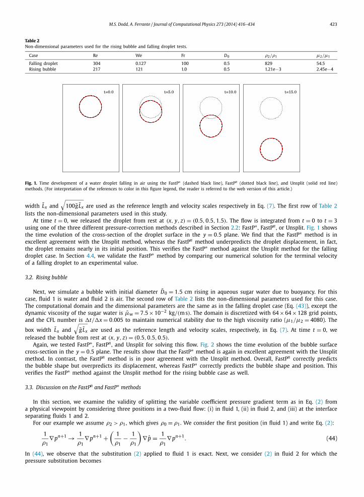
Fig. 1. Time development of a water droplet falling in air using the FastP∗ (dashed black line), FastPn (dotted black line), and Unsplit (solid red line) methods. (For interpretation of the references to color in this figure legend, the reader is referred to the web version of this article.)

width Lx and √

100g Lx are used as the reference length and velocity scales respectively in Eq. (7). The first row of Table 2lists the non-dimensional parameters used in this study.

At time t = 0, we released the droplet from rest at (x, y, z) = (0.5, 0.5, 1.5). The flow is integrated from t = 0 to t = 3using one of the three different pressure-correction methods described in Section 2.2: FastP∗, FastPn , or Unsplit. Fig. 1 shows the time evolution of the cross-section of the droplet surface in the y = 0.5 plane. We find that the FastP∗ method is in excellent agreement with the Unsplit method, whereas the FastPn method underpredicts the droplet displacement, in fact, the droplet remains nearly in its initial position. This verifies the FastP∗ method against the Unsplit method for the falling droplet case. In Section 4.4, we validate the FastP∗ method by comparing our numerical solution for the terminal velocity of a falling droplet to an experimental value.

3.2. Rising bubble

Next, we simulate a bubble with initial diameter D0 = 1.5 cm rising in aqueous sugar water due to buoyancy. For this case, fluid 1 is water and fluid 2 is air. The second row of Table 2 lists the non-dimensional parameters used for this case. The computational domain and the dimensional parameters are the same as in the falling droplet case (Eq. (43)), except the dynamic viscosity of the sugar water is μw = 7.5 × 10−2 kg/(m s). The domain is discretized with 64 × 64 × 128 grid points, and the CFL number is �t/�x = 0.005 to maintain numerical stability due to the high viscosity ratio (μ1/μ2 = 4080). The

box width Lx and √

g Lx are used as the reference length and velocity scales, respectively, in Eq. (7). At time t = 0, we released the bubble from rest at (x, y, z) = (0.5, 0.5, 0.5).

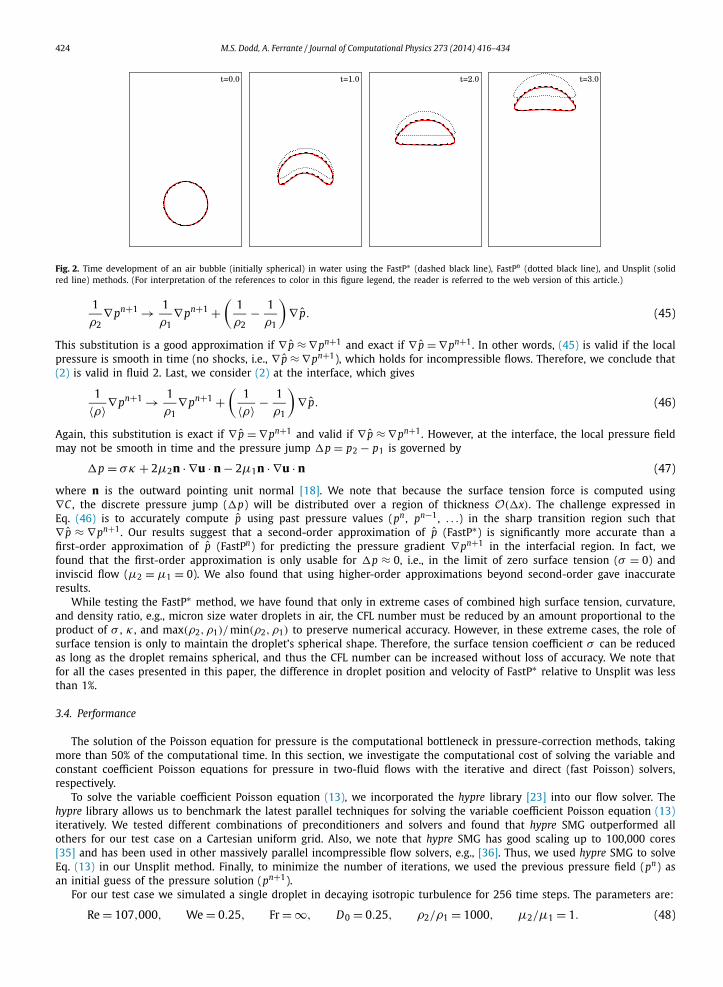
Again, we tested FastP∗, FastPn , and Unsplit for solving this flow. Fig. 2 shows the time evolution of the bubble surface cross-section in the y = 0.5 plane. The results show that the FastP∗ method is again in excellent agreement with the Unsplit method. In contrast, the FastPn method is in poor agreement with the Unsplit method. Overall, FastPn correctly predicts the bubble shape but overpredicts its displacement, whereas FastP∗ correctly predicts the bubble shape and position. This verifies the FastP∗ method against the Unsplit method for the rising bubble case as well.

3.3. Discussion on the FastPn and FastP∗ methods

In this section, we examine the validity of splitting the variable coefficient pressure gradient term as in Eq. (2) from a physical viewpoint by considering three positions in a two-fluid flow: (i) in fluid 1, (ii) in fluid 2, and (iii) at the interface separating fluids 1 and 2.

For our example we assume ρ2 > ρ1, which gives ρ0 = ρ1. We consider the first position (in fluid 1) and write Eq. (2):

1

ρ1∇pn+1 → 1

ρ1∇pn+1 +

(1

ρ1− 1

ρ1

)∇ p = 1

ρ1∇pn+1. (44)

In (44), we observe that the substitution (2) applied to fluid 1 is exact. Next, we consider (2) in fluid 2 for which the pressure substitution becomes

424 M.S. Dodd, A. Ferrante / Journal of Computational Physics 273 (2014) 416–434

Fig. 2. Time development of an air bubble (initially spherical) in water using the FastP∗ (dashed black line), FastPn (dotted black line), and Unsplit (solid red line) methods. (For interpretation of the references to color in this figure legend, the reader is referred to the web version of this article.)

1

ρ2∇pn+1 → 1

ρ1∇pn+1 +

(1

ρ2− 1

ρ1

)∇ p. (45)

This substitution is a good approximation if ∇ p ≈ ∇pn+1 and exact if ∇ p = ∇pn+1. In other words, (45) is valid if the local pressure is smooth in time (no shocks, i.e., ∇ p ≈ ∇pn+1), which holds for incompressible flows. Therefore, we conclude that (2) is valid in fluid 2. Last, we consider (2) at the interface, which gives

1

〈ρ〉∇pn+1 → 1

ρ1∇pn+1 +

(1

〈ρ〉 − 1

ρ1

)∇ p. (46)

Again, this substitution is exact if ∇ p = ∇pn+1 and valid if ∇ p ≈ ∇pn+1. However, at the interface, the local pressure field may not be smooth in time and the pressure jump �p = p2 − p1 is governed by

�p = σκ + 2μ2n · ∇u · n − 2μ1n · ∇u · n (47)

where n is the outward pointing unit normal [18]. We note that because the surface tension force is computed using ∇C , the discrete pressure jump (�p) will be distributed over a region of thickness O(�x). The challenge expressed in Eq. (46) is to accurately compute p using past pressure values (pn , pn−1, . . .) in the sharp transition region such that ∇ p ≈ ∇pn+1. Our results suggest that a second-order approximation of p (FastP∗) is significantly more accurate than a first-order approximation of p (FastPn) for predicting the pressure gradient ∇pn+1 in the interfacial region. In fact, we found that the first-order approximation is only usable for �p ≈ 0, i.e., in the limit of zero surface tension (σ = 0) and inviscid flow (μ2 = μ1 = 0). We also found that using higher-order approximations beyond second-order gave inaccurate results.

While testing the FastP∗ method, we have found that only in extreme cases of combined high surface tension, curvature, and density ratio, e.g., micron size water droplets in air, the CFL number must be reduced by an amount proportional to the product of σ , κ , and max(ρ2, ρ1)/ min(ρ2, ρ1) to preserve numerical accuracy. However, in these extreme cases, the role of surface tension is only to maintain the droplet’s spherical shape. Therefore, the surface tension coefficient σ can be reduced as long as the droplet remains spherical, and thus the CFL number can be increased without loss of accuracy. We note that for all the cases presented in this paper, the difference in droplet position and velocity of FastP∗ relative to Unsplit was less than 1%.

3.4. Performance

The solution of the Poisson equation for pressure is the computational bottleneck in pressure-correction methods, taking more than 50% of the computational time. In this section, we investigate the computational cost of solving the variable and constant coefficient Poisson equations for pressure in two-fluid flows with the iterative and direct (fast Poisson) solvers, respectively.

To solve the variable coefficient Poisson equation (13), we incorporated the hypre library [23] into our flow solver. The hypre library allows us to benchmark the latest parallel techniques for solving the variable coefficient Poisson equation (13)iteratively. We tested different combinations of preconditioners and solvers and found that hypre SMG outperformed all others for our test case on a Cartesian uniform grid. Also, we note that hypre SMG has good scaling up to 100,000 cores [35] and has been used in other massively parallel incompressible flow solvers, e.g., [36]. Thus, we used hypre SMG to solve Eq. (13) in our Unsplit method. Finally, to minimize the number of iterations, we used the previous pressure field (pn) as an initial guess of the pressure solution (pn+1).

For our test case we simulated a single droplet in decaying isotropic turbulence for 256 time steps. The parameters are:

Re = 107,000, We = 0.25, Fr = ∞, D0 = 0.25, ρ2/ρ1 = 1000, μ2/μ1 = 1. (48)

M.S. Dodd, A. Ferrante / Journal of Computational Physics 273 (2014) 416–434 425

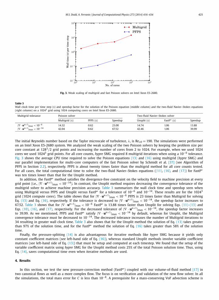
Fig. 3. Weak scaling of multigrid and fast Poisson solvers on Intel Xeon E5-2680.

Table 3Wall clock time per time step (s) and speedup factor for the solution of the Poisson equation (middle column) and the two-fluid Navier–Stokes equations (right column) on a 10243 grid using 1024 computing cores on Intel Xeon E5-2680.

Multigrid tolerance Poisson solver Two-fluid Navier–Stokes solver

Multigrid (s) PFPS (s) Speedup Unsplit (s) FastP∗ (s) Speedup

|∇ · un+1|max < 10−6 14.32 0.62 23.00 14.74 1.06 13.88|∇ · un+1|max < 10−14 42.04 0.62 67.52 42.46 1.06 39.99

The initial Reynolds number based on the Taylor microscale of turbulence, λ, is Reλ0 = 190. The simulations were performed on an Intel Xeon E5-2680 system. We analyzed the weak scaling of the two Poisson solvers by keeping the problem size per core constant at 1283/2 grid points and increasing the number of cores from 2 to 1024. For example, when we used 1024 cores we used 10243 grid points. For all core counts, hypre SMG required 8 multigrid iterations when using a 10−6 tolerance. Fig. 3 shows the average CPU time required to solve the Poisson equations (13) and (16) using multigrid (hypre SMG) and our parallel implementation for multi-core computers of the fast Poisson solver by Schmidt et al. [37] (see Algorithm of PFPS in Section 2.2), respectively. PFPS is about twenty times faster than the multigrid method for all core counts tested. For all cases, the total computational time to solve the two-fluid Navier–Stokes equations ((11), (16), and (17)) for FastP∗was ten times lower than that for the Unsplit method.

In addition, the FastP∗ method satisfies the divergence-free constraint on the velocity field to machine precision at every grid point (i.e., |∇ · un+1|max < 10−14). In contrast, the Unsplit method requires decreasing the convergence tolerance of the multigrid solver to achieve machine precision accuracy. Table 3 summarizes the wall clock time and speedup seen when using Multigrid versus PFPS and Unsplit versus FastP∗ for a tolerance of 10−6 and 10−14. These results are for the 10243

grid (1024 compute cores). The table shows that for |∇ · un+1|max < 10−6 PFPS is 23 times faster than Multigrid for solving Eq. (13) and Eq. (16), respectively. If the tolerance is decreased to |∇ · un+1|max < 10−14, the speedup factor increases to 67.52. Table 3 shows that for |∇ · un+1|max < 10−6 FastP∗ is 13.88 times faster than Unsplit for solving Eqs. (11)–(13) and Eqs. (10), (16), and (17), respectively. For the decreased tolerance of |∇ · un+1|max < 10−14, the speedup factor increases to 39.99. As we mentioned, PFPS and FastP∗ satisfy |∇ · un+1|max < 10−14 by default, whereas for Unsplit, the Multigrid convergence tolerance must be decreased to 10−14. The decreased tolerance increases the number of Multigrid iterations to 34 resulting in greater wall clock time. Table 3 also shows that for the Unsplit method the solution of Eq. (13) takes greater than 97% of the solution time, and for the FastP∗ method the solution of Eq. (16) takes greater than 58% of the solution time.

Finally, the pressure-splitting (14) is also advantageous for iterative methods like hypre SMG because it yields only constant coefficient matrices (see left-hand side of Eq. (16)), whereas standard Unsplit methods involve variable coefficient matrices (see left-hand side of Eq. (13)) that must be setup and computed at each timestep. We found that the setup of the variable coefficient matrix using hypre SMG for the Unsplit method costs 25% of the total Poisson solution time. Thus, using Eq. (14), saves computational time even when iterative methods are used.

4. Results

In this section, we test the new pressure-correction method (FastP∗) coupled with our volume-of-fluid method [17] in two canonical flows as well as a more complex flow. The focus is on verification and validation of the new flow solver. In all the simulations, the total mass error for C is less than 10−8. A prerequisite for a mass-conserving VoF advection scheme is

426 M.S. Dodd, A. Ferrante / Journal of Computational Physics 273 (2014) 416–434

Table 4Temporal errors and convergence rate for velocity (u) and pressure (p) in the Taylor–Green vortex flow with a fluid 2 cylinder centered in the domain.

E4�t,2�t E2�t,�t Rate

u 5.94e−8 1.53e−8 1.96p 3.67e−6 1.84e−6 0.99

Table 5Spatial errors and convergence rate for velocity (u) and pressure (p) in the Taylor–Green vortex flow with a fluid 2 cylinder centered in the domain.

E4�x,2�x E2�x,�x Rate

u 6.08e−3 1.51e−3 2.01p 1.04e−1 2.63e−2 1.99

a divergence-free velocity field. Therefore, another advantage of the FastP∗ is that by solving Eq. (16) directly, the resulting discrete velocity field (Eq. (17)) is divergence free to machine precision.

4.1. Convergence rates

We assess the solver’s numerical accuracy by computing its spatial and temporal convergence rates. Special consideration is needed when computing the temporal accuracy of the coupled pressure-correction/VoF flow solver because the VoF advection method uses first-order forward Euler to integrate Eq. (41) in time, which is the standard for geometrical VoF methods [30, Chapter 5, p. 108]. In Section 4.1.1, we compute the convergence rates independent of the method used to advect the interface by turning the VoF advection off such that C = C(x) for all times. In Section 4.1.2 we present the convergence rates with the VoF advection turned on, i.e., C = C(x, t).

4.1.1. Convergence rates without VoF advectionWe simulate a fluid cylinder (fluid 2) centered in a two-dimensional Taylor–Green vortex flow (fluid 1) [38]. The non-

dimensional parameters for the flow are:

Re = 200, We = ∞, Fr = ∞, D = 0.25, ρ2/ρ1 = 10, μ2/μ1 = 10. (49)

The fluid velocity in the interior of the cylinder was set equal to the local Taylor–Green vortex velocity at time t = 0. In time, the vorticity of both fluids decays owing to viscous diffusion.

We simulated the flow on a computational mesh of 2562 points. The smallest time step used was �t = 4.88e−5 and the number of time steps to reach tmax = 0.05 was Nt = 1024. To evaluate the temporal convergence rate of the solver, the time step was increased to 2�t and 4�t (Nt = 512 and 256) and we computed the error between successive solutions. The L2 error E for generic flow variable ξ is computed as:

E2�t,�t = 1

NxN y

√√√√√ Nx∑i=1

N y∑j=1

(ξ

(i, j)2�t − ξ

(i, j)�t

)2. (50)

Table 4 shows the error between successive time steps and the convergence rate. The convergence rate of the u-component of velocity is 1.96, therefore the velocity is second-order in time. The convergence rate of pressure is 0.99, thus it is first-order in time. Second-order pressure convergence in time can be achieved if �t � Re�x2 and periodic boundary conditions are applied [39]. The condition �t � Re�x2 is unlikely to be satisfied in high Reynolds number (Re) turbu-lent flows. Therefore, the accuracy of the pressure is expected to be first-order for high Re flows and cannot be improved by switching to semi-implicit or implicit time integration, e.g. Adams–Bashforth Crank–Nicolson scheme (see Appendix A) when using the pressure-correction method presented. There is a method in which the pressure is 3/2-order accurate in time, but it was developed for single-phase flow [40].

Next, we assess the spatial accuracy of the solver by successively refining the grid and computing the convergence rate of the solution. We again solve the above described Taylor–Green vortex case. We used grids with 322, 642, and 1282 points, and we used CFL number �t/�x = 0.001 such that temporal errors are small. Table 5 shows the error between successive grid refinements and the convergence rate. Both velocity and pressure have a second-order convergence rate (2.01 and 1.99, respectively), which is consistent with our central difference discretization in space. In summary, FastP∗ is first-order in time for the pressure, second-order in time for the velocity, and second-order in space for both pressure and velocity.

4.1.2. Convergence rates with VoF advectionWe assess the coupled FastP∗/VoF flow solver’s numerical accuracy by computing the spatial and temporal convergence

rates. The test problem is a two-dimensional capillary wave in a periodic domain. The non-dimensional parameters for the

M.S. Dodd, A. Ferrante / Journal of Computational Physics 273 (2014) 416–434 427

Table 6Temporal errors and convergence rate for velocity component (u), pressure (p), and volume fraction (C ) in the 2-D capillary wave flow.

E4�t,2�t E2�t,�t Rate

u 7.32e−9 3.91e−9 0.90p 4.67e−7 2.32e−7 1.01C 7.38e−8 3.58e−8 1.04

Table 7Spatial errors and convergence rate for velocity component (u), pressure (p), and volume fraction (C ) in the 2-D capillary wave flow.

E4�x,2�x E2�x,�x Rate

u 2.52e−5 6.33e−6 1.99p 1.68e−3 4.52e−4 1.89C 1.88e−3 5.14e−4 1.87

flow are:

Re = 500, We = 1.0, Fr = ∞, H0 = 0.05, ρ2/ρ1 = 20, μ2/μ1 = 20. (51)

We do not use Prosperetti’s solution [41] for computing the convergence rate of the error because it was derived for fluids of infinite depth and we are using a periodic domain. Instead, we compute the temporal convergence rate by comparing the error in the flow solution computed using successively smaller time steps �t .

We simulated the flow on a 2562 grid. The flow was integrated up to tmax = 0.0625, and the smallest time step used was �t = 4.88e−5 (Nt = 1280). To evaluate the temporal convergence rate of the solver, the time step was increased to 2�t and 4�t (Nt = 640 and 320), and we computed the error between successive solutions. The L2 error E for generic flow variable ξ (u, p, or C ) is computed using Eq. (50).

Table 6 shows the error between successive time step sizes and the convergence rate for u, p, and C . The convergence rate of u is 0.90, which is slightly less than first-order. The convergence rate of pressure and the volume fraction are 1.01 and 1.04 respectively, thus it is first-order. Overall, the coupled flow solver is first-order accurate in time. The cause of the first-order temporal accuracy, despite using second-order Adams–Bashforth in Eq. (11), is that the volume fraction is advected by first integrating Eq. (41) in each cell and then integrating in time using forward Euler [21,17]. To overcome this limitation, higher order VoF advection methods have been employed, however they are inadequate for long time simulations [30, Chapter 4, p. 80]. The flow solver could be made fully second-order by using a second-order in time method to advect the interface.

Next, we assess the spatial accuracy of the solver by successively refining the grid and computing the convergence rate of the solution. We solve the above described capillary wave case on 322, 642, and 1282 grids. The CFL number is held constant and set to �t/�x = 0.0025. Table 7 shows the error between successive grid refinements and the convergence rate. The velocity, pressure, and volume fraction all have nearly second-order convergence rates (1.99, 1.89, and 1.87, respectively), which is consistent with our central difference discretization in space (Section 2.2.1) and second-order VoF method [17]. We conclude that the coupled FastP∗/VoF method is second-order accurate in space.

4.2. Conservation of momentum and kinetic energy

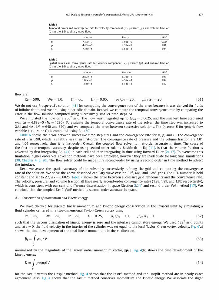
We have checked for discrete linear momentum and kinetic energy conservation in the inviscid limit by simulating a fluid cylinder centered in a two-dimensional Taylor–Green vortex using

Re = ∞, We = ∞, Fr = ∞, D = 0.25, ρ2/ρ1 = 10, μ2/μ1 = 1. (52)

such that the viscous dissipation of kinetic energy is zero and the interface cannot store energy. We used 1282 grid points and, at t = 0, the fluid velocity in the interior of the cylinder was set equal to the local Taylor–Green vortex velocity. Fig. 4(a) shows the time development of the total linear momentum in the xi direction,

pi =∫V

ρuidV (53)

normalized by the magnitude of the largest initial momentum vector, ‖p0‖. Fig. 4(b) shows the time development of the kinetic energy

K =∫V

ρuiuidV (54)

for the FastP∗ versus the Unsplit method. Fig. 4 shows that the FastP∗ method and the Unsplit method are in nearly exact agreement. Also, Fig. 4 shows that the FastP∗ method conserves momentum and kinetic energy. We associate the slight

428 M.S. Dodd, A. Ferrante / Journal of Computational Physics 273 (2014) 416–434

Fig. 4. Time development of (a) the x- (black), y- (red), and z-component (blue) of momentum using the FastP∗ and Unsplit method and (b) the kinetic energy using the FastP∗ and the Unsplit method. (For interpretation of the references to color in this figure legend, the reader is referred to the web version of this article.)

increase in K seen for t > 4 to the increasing deformation of the cylinder interface, and thus decreasing cylinder resolution, D/�x. For t > 4, parts of the cylinder interface are under resolved (D/�x < 6) which decreases the accuracy of the VoF advection algorithm.

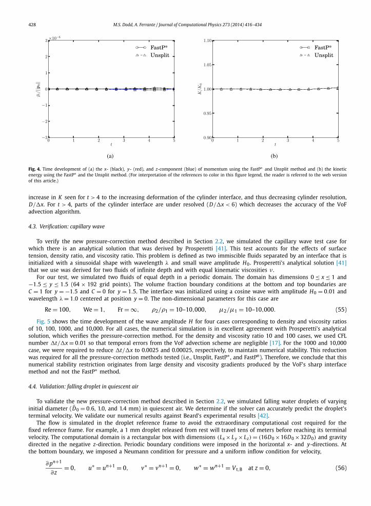
4.3. Verification: capillary wave

To verify the new pressure-correction method described in Section 2.2, we simulated the capillary wave test case for which there is an analytical solution that was derived by Prosperetti [41]. This test accounts for the effects of surface tension, density ratio, and viscosity ratio. This problem is defined as two immiscible fluids separated by an interface that is initialized with a sinusoidal shape with wavelength λ and small wave amplitude H0. Prosperetti’s analytical solution [41]that we use was derived for two fluids of infinite depth and with equal kinematic viscosities ν .

For our test, we simulated two fluids of equal depth in a periodic domain. The domain has dimensions 0 ≤ x ≤ 1 and −1.5 ≤ y ≤ 1.5 (64 × 192 grid points). The volume fraction boundary conditions at the bottom and top boundaries are C = 1 for y = −1.5 and C = 0 for y = 1.5. The interface was initialized using a cosine wave with amplitude H0 = 0.01 and wavelength λ = 1.0 centered at position y = 0. The non-dimensional parameters for this case are

Re = 100, We = 1, Fr = ∞, ρ2/ρ1 = 10–10,000, μ2/μ1 = 10–10,000. (55)

Fig. 5 shows the time development of the wave amplitude H for four cases corresponding to density and viscosity ratios of 10, 100, 1000, and 10,000. For all cases, the numerical simulation is in excellent agreement with Prosperetti’s analytical solution, which verifies the pressure-correction method. For the density and viscosity ratio 10 and 100 cases, we used CFL number �t/�x = 0.01 so that temporal errors from the VoF advection scheme are negligible [17]. For the 1000 and 10,000 case, we were required to reduce �t/�x to 0.0025 and 0.00025, respectively, to maintain numerical stability. This reduction was required for all the pressure-correction methods tested (i.e., Unsplit, FastP∗ , and FastPn). Therefore, we conclude that this numerical stability restriction originates from large density and viscosity gradients produced by the VoF’s sharp interface method and not the FastP∗ method.

4.4. Validation: falling droplet in quiescent air

To validate the new pressure-correction method described in Section 2.2, we simulated falling water droplets of varying initial diameter (D0 = 0.6, 1.0, and 1.4 mm) in quiescent air. We determine if the solver can accurately predict the droplet’s terminal velocity. We validate our numerical results against Beard’s experimental results [42].

The flow is simulated in the droplet reference frame to avoid the extraordinary computational cost required for the fixed reference frame. For example, a 1 mm droplet released from rest will travel tens of meters before reaching its terminal velocity. The computational domain is a rectangular box with dimensions (Lx × L y × Lz) = (16D0 ×16D0 ×32D0) and gravity directed in the negative z-direction. Periodic boundary conditions were imposed in the horizontal x- and y-directions. At the bottom boundary, we imposed a Neumann condition for pressure and a uniform inflow condition for velocity,

∂ pn+1

= 0, u∗ = un+1 = 0, v∗ = vn+1 = 0, w∗ = wn+1 = V t,B at z = 0, (56)

∂z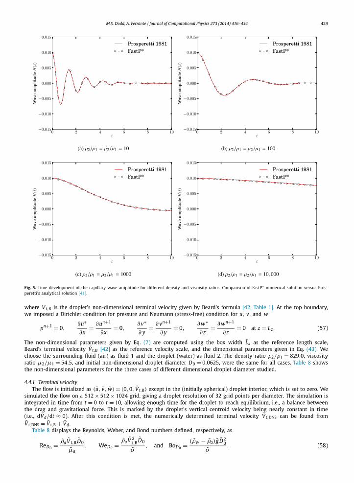

M.S. Dodd, A. Ferrante / Journal of Computational Physics 273 (2014) 416–434 429

Fig. 5. Time development of the capillary wave amplitude for different density and viscosity ratios. Comparison of FastP∗ numerical solution versus Pros-peretti’s analytical solution [41].

where V t,B is the droplet’s non-dimensional terminal velocity given by Beard’s formula [42, Table 1]. At the top boundary, we imposed a Dirichlet condition for pressure and Neumann (stress-free) condition for u, v , and w

pn+1 = 0,∂u∗

∂x= ∂un+1

∂x= 0,

∂v∗

∂ y= ∂vn+1

∂ y= 0,

∂ w∗

∂z= ∂ wn+1

∂z= 0 at z = Lz. (57)

The non-dimensional parameters given by Eq. (7) are computed using the box width Lx as the reference length scale, Beard’s terminal velocity V t,B [42] as the reference velocity scale, and the dimensional parameters given in Eq. (43). We choose the surrounding fluid (air) as fluid 1 and the droplet (water) as fluid 2. The density ratio ρ2/ρ1 = 829.0, viscosity ratio μ2/μ1 = 54.5, and initial non-dimensional droplet diameter D0 = 0.0625, were the same for all cases. Table 8 shows the non-dimensional parameters for the three cases of different dimensional droplet diameter studied.

4.4.1. Terminal velocityThe flow is initialized as (u, v, w) = (0, 0, V t,B) except in the (initially spherical) droplet interior, which is set to zero. We

simulated the flow on a 512 × 512 × 1024 grid, giving a droplet resolution of 32 grid points per diameter. The simulation is integrated in time from t = 0 to t = 10, allowing enough time for the droplet to reach equilibrium, i.e., a balance between the drag and gravitational force. This is marked by the droplet’s vertical centroid velocity being nearly constant in time (i.e., dVd/dt ≈ 0). After this condition is met, the numerically determined terminal velocity V t,DNS can be found from V t,DNS = V t,B + Vd .

Table 8 displays the Reynolds, Weber, and Bond numbers defined, respectively, as

ReD0 = ρa V t,B D0, WeD0 = ρa V 2

t,B D0, and BoD0 = (ρw − ρa)g D2

0 . (58)

μa σ σ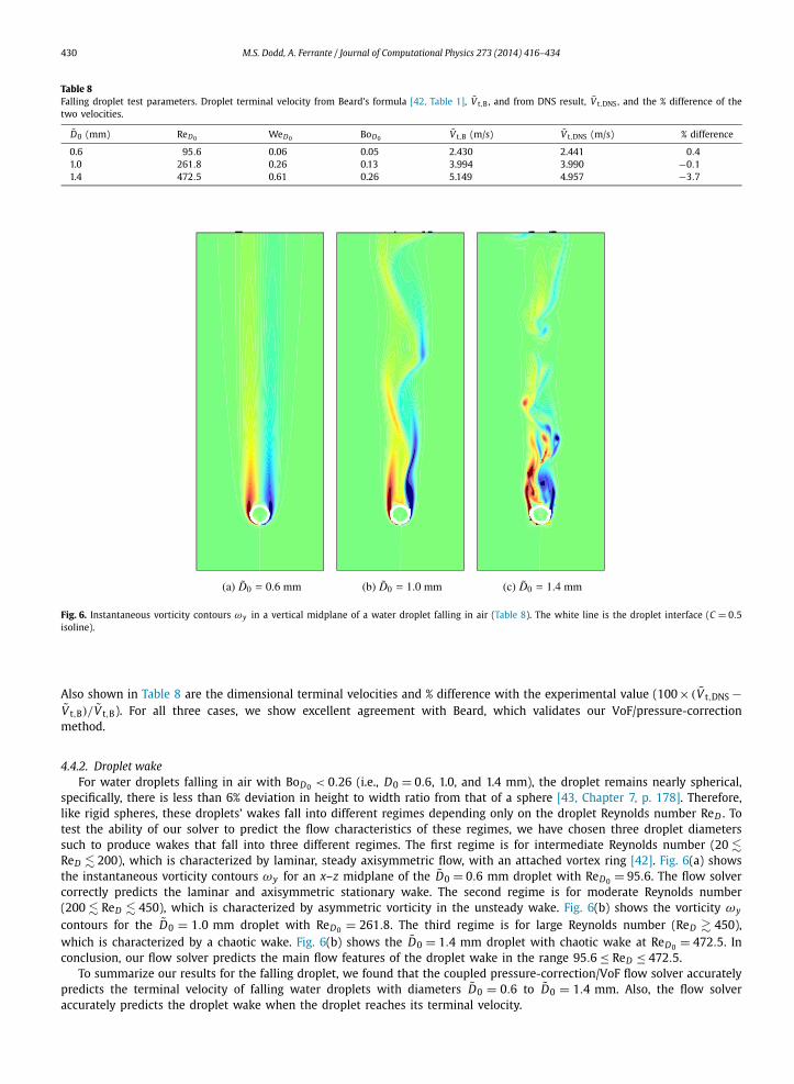

430 M.S. Dodd, A. Ferrante / Journal of Computational Physics 273 (2014) 416–434

Table 8Falling droplet test parameters. Droplet terminal velocity from Beard’s formula [42, Table 1], V t,B, and from DNS result, V t,DNS, and the % difference of the two velocities.

D0 (mm) ReD0 WeD0 BoD0 V t,B (m/s) V t,DNS (m/s) % difference

0.6 95.6 0.06 0.05 2.430 2.441 0.41.0 261.8 0.26 0.13 3.994 3.990 −0.11.4 472.5 0.61 0.26 5.149 4.957 −3.7

Fig. 6. Instantaneous vorticity contours ωy in a vertical midplane of a water droplet falling in air (Table 8). The white line is the droplet interface (C = 0.5isoline).

Also shown in Table 8 are the dimensional terminal velocities and % difference with the experimental value (100 × (V t,DNS −V t,B)/V t,B). For all three cases, we show excellent agreement with Beard, which validates our VoF/pressure-correction method.

4.4.2. Droplet wakeFor water droplets falling in air with BoD0 < 0.26 (i.e., D0 = 0.6, 1.0, and 1.4 mm), the droplet remains nearly spherical,

specifically, there is less than 6% deviation in height to width ratio from that of a sphere [43, Chapter 7, p. 178]. Therefore, like rigid spheres, these droplets’ wakes fall into different regimes depending only on the droplet Reynolds number ReD . To test the ability of our solver to predict the flow characteristics of these regimes, we have chosen three droplet diameters such to produce wakes that fall into three different regimes. The first regime is for intermediate Reynolds number (20 �ReD � 200), which is characterized by laminar, steady axisymmetric flow, with an attached vortex ring [42]. Fig. 6(a) shows the instantaneous vorticity contours ωy for an x–z midplane of the D0 = 0.6 mm droplet with ReD0 = 95.6. The flow solver correctly predicts the laminar and axisymmetric stationary wake. The second regime is for moderate Reynolds number (200 � ReD � 450), which is characterized by asymmetric vorticity in the unsteady wake. Fig. 6(b) shows the vorticity ωy

contours for the D0 = 1.0 mm droplet with ReD0 = 261.8. The third regime is for large Reynolds number (ReD � 450), which is characterized by a chaotic wake. Fig. 6(b) shows the D0 = 1.4 mm droplet with chaotic wake at ReD0 = 472.5. In conclusion, our flow solver predicts the main flow features of the droplet wake in the range 95.6 ≤ ReD ≤ 472.5.

To summarize our results for the falling droplet, we found that the coupled pressure-correction/VoF flow solver accurately predicts the terminal velocity of falling water droplets with diameters D0 = 0.6 to D0 = 1.4 mm. Also, the flow solver accurately predicts the droplet wake when the droplet reaches its terminal velocity.

M.S. Dodd, A. Ferrante / Journal of Computational Physics 273 (2014) 416–434 431

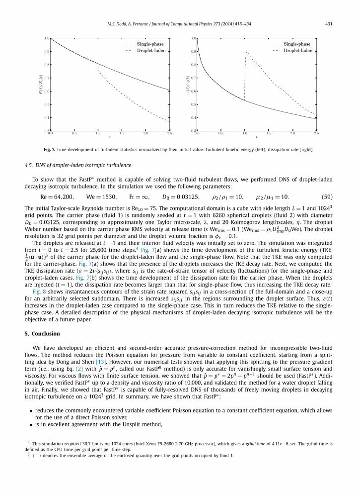
Fig. 7. Time development of turbulent statistics normalized by their initial value. Turbulent kinetic energy (left); dissipation rate (right).

4.5. DNS of droplet-laden isotropic turbulence

To show that the FastP∗ method is capable of solving two-fluid turbulent flows, we performed DNS of droplet-laden decaying isotropic turbulence. In the simulation we used the following parameters:

Re = 64,200, We = 1530, Fr = ∞, D0 = 0.03125, ρ2/ρ1 = 10, μ2/μ1 = 10. (59)

The initial Taylor-scale Reynolds number is Reλ0 = 75. The computational domain is a cube with side length L = 1 and 10243

grid points. The carrier phase (fluid 1) is randomly seeded at t = 1 with 6260 spherical droplets (fluid 2) with diameter D0 = 0.03125, corresponding to approximately one Taylor microscale, λ, and 20 Kolmogorov lengthscales, η. The droplet Weber number based on the carrier phase RMS velocity at release time is Werms = 0.1 (Werms = ρ1U 2

rms D0We). The droplet resolution is 32 grid points per diameter and the droplet volume fraction is φv = 0.1.

The droplets are released at t = 1 and their interior fluid velocity was initially set to zero. The simulation was integrated from t = 0 to t = 2.5 for 25,600 time steps.4 Fig. 7(a) shows the time development of the turbulent kinetic energy (TKE, 12 〈u · u〉)5 of the carrier phase for the droplet-laden flow and the single-phase flow. Note that the TKE was only computed for the carrier-phase. Fig. 7(a) shows that the presence of the droplets increases the TKE decay rate. Next, we computed the TKE dissipation rate (ε = 2ν〈si j si j〉, where si j is the rate-of-strain tensor of velocity fluctuations) for the single-phase and droplet-laden cases. Fig. 7(b) shows the time development of the dissipation rate for the carrier phase. When the droplets are injected (t = 1), the dissipation rate becomes larger than that for single-phase flow, thus increasing the TKE decay rate.

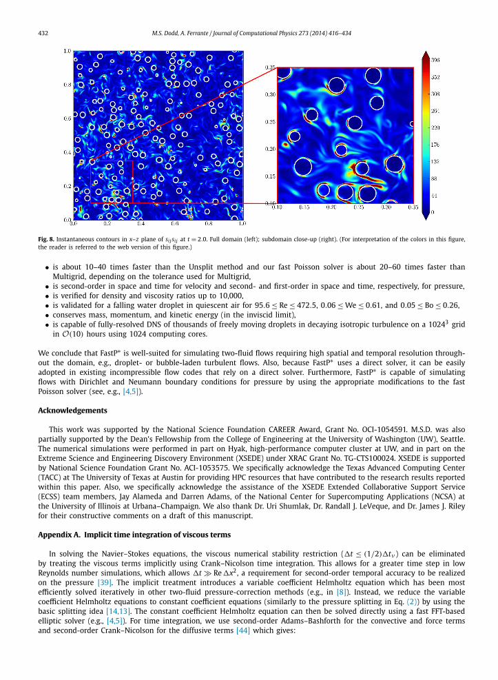
Fig. 8 shows instantaneous contours of the strain rate squared si j si j in a cross-section of the full-domain and a close-up for an arbitrarily selected subdomain. There is increased si j si j in the regions surrounding the droplet surface. Thus, ε(t)increases in the droplet-laden case compared to the single-phase case. This in turn reduces the TKE relative to the single-phase case. A detailed description of the physical mechanisms of droplet-laden decaying isotropic turbulence will be the objective of a future paper.

5. Conclusion

We have developed an efficient and second-order accurate pressure-correction method for incompressible two-fluid flows. The method reduces the Poisson equation for pressure from variable to constant coefficient, starting from a split-ting idea by Dong and Shen [13]. However, our numerical tests showed that applying this splitting to the pressure gradient term (i.e., using Eq. (2) with p = pn , called our FastPn method) is only accurate for vanishingly small surface tension and viscosity. For viscous flows with finite surface tension, we showed that p = p∗ = 2pn − pn−1 should be used (FastP∗). Addi-tionally, we verified FastP∗ up to a density and viscosity ratio of 10,000, and validated the method for a water droplet falling in air. Finally, we showed that FastP∗ is capable of fully-resolved DNS of thousands of freely moving droplets in decaying isotropic turbulence on a 10243 grid. In summary, we have shown that FastP∗:

• reduces the commonly encountered variable coefficient Poisson equation to a constant coefficient equation, which allows for the use of a direct Poisson solver,

• is in excellent agreement with the Unsplit method,

4 This simulation required 30.7 hours on 1024 cores (Intel Xeon E5-2680 2.70 GHz processor), which gives a grind time of 4.11e−6 sec. The grind time is defined as the CPU time per grid point per time step.

5 〈. . .〉 denotes the ensemble average of the enclosed quantity over the grid points occupied by fluid 1.

432 M.S. Dodd, A. Ferrante / Journal of Computational Physics 273 (2014) 416–434

Fig. 8. Instantaneous contours in x–z plane of si j si j at t = 2.0. Full domain (left); subdomain close-up (right). (For interpretation of the colors in this figure, the reader is referred to the web version of this figure.)

• is about 10–40 times faster than the Unsplit method and our fast Poisson solver is about 20–60 times faster than Multigrid, depending on the tolerance used for Multigrid,

• is second-order in space and time for velocity and second- and first-order in space and time, respectively, for pressure,• is verified for density and viscosity ratios up to 10,000,• is validated for a falling water droplet in quiescent air for 95.6 ≤ Re ≤ 472.5, 0.06 ≤ We ≤ 0.61, and 0.05 ≤ Bo ≤ 0.26,• conserves mass, momentum, and kinetic energy (in the inviscid limit),• is capable of fully-resolved DNS of thousands of freely moving droplets in decaying isotropic turbulence on a 10243 grid

in O(10) hours using 1024 computing cores.

We conclude that FastP∗ is well-suited for simulating two-fluid flows requiring high spatial and temporal resolution through-out the domain, e.g., droplet- or bubble-laden turbulent flows. Also, because FastP∗ uses a direct solver, it can be easily adopted in existing incompressible flow codes that rely on a direct solver. Furthermore, FastP∗ is capable of simulating flows with Dirichlet and Neumann boundary conditions for pressure by using the appropriate modifications to the fast Poisson solver (see, e.g., [4,5]).

Acknowledgements

This work was supported by the National Science Foundation CAREER Award, Grant No. OCI-1054591. M.S.D. was also partially supported by the Dean’s Fellowship from the College of Engineering at the University of Washington (UW), Seattle. The numerical simulations were performed in part on Hyak, high-performance computer cluster at UW, and in part on the Extreme Science and Engineering Discovery Environment (XSEDE) under XRAC Grant No. TG-CTS100024. XSEDE is supported by National Science Foundation Grant No. ACI-1053575. We specifically acknowledge the Texas Advanced Computing Center (TACC) at The University of Texas at Austin for providing HPC resources that have contributed to the research results reported within this paper. Also, we specifically acknowledge the assistance of the XSEDE Extended Collaborative Support Service (ECSS) team members, Jay Alameda and Darren Adams, of the National Center for Supercomputing Applications (NCSA) at the University of Illinois at Urbana–Champaign. We also thank Dr. Uri Shumlak, Dr. Randall J. LeVeque, and Dr. James J. Riley for their constructive comments on a draft of this manuscript.

Appendix A. Implicit time integration of viscous terms

In solving the Navier–Stokes equations, the viscous numerical stability restriction (�t ≤ (1/2)�tν ) can be eliminated by treating the viscous terms implicitly using Crank–Nicolson time integration. This allows for a greater time step in low Reynolds number simulations, which allows �t � Re�x2, a requirement for second-order temporal accuracy to be realized on the pressure [39]. The implicit treatment introduces a variable coefficient Helmholtz equation which has been most efficiently solved iteratively in other two-fluid pressure-correction methods (e.g., in [8]). Instead, we reduce the variable coefficient Helmholtz equations to constant coefficient equations (similarly to the pressure splitting in Eq. (2)) by using the basic splitting idea [14,13]. The constant coefficient Helmholtz equation can then be solved directly using a fast FFT-based elliptic solver (e.g., [4,5]). For time integration, we use second-order Adams–Bashforth for the convective and force terms and second-order Crank–Nicolson for the diffusive terms [44] which gives:

M.S. Dodd, A. Ferrante / Journal of Computational Physics 273 (2014) 416–434 433

u∗ − un

�t= 1

2

(3Hn − Hn−1) + 1

2

1

Re

1

ρn+1

[∇ · (μn+1D(un)) + ∇ · (μn+1D

(u∗))] (A.1)

with

Hk = −∇ · (ukuk) + 1

ρk+1

1

Wefk+1σ

D(uk) = (∇uk + (∇uk)T )

. (A.2)

The last viscous term in Eq. (A.1) with variable coefficients is split into a constant part and a variable part, and the constant part is treated implicitly and the variable part explicitly [13], i.e.,

1

ρn+1∇ · (μn+1D

(u∗)) → ν0∇2u∗ + 1

ρn+1∇ · (μn+1D

(un)) − ν0∇2un (A.3)

where ν0 = 12 (

μ1ρ1

+ μ2ρ2

). Unlike the pressure field, the velocity field is continuous across the interface, thus, we do not need to linearly extrapolate un in time as we did for the pressure in (14) (see Section 3.3). The substitution in (A.3) is consistent because we recover the constant-property Navier–Stokes equations if we set μ1 = ρ1 = μ2 = ρ2 = 1. Substituting Eq. (A.3)into Eq. (A.1) gives:

u∗ − un

�t= 1

2

(3Hn − Hn−1) + 1

Re

1

ρn+1

[∇ · (μn+1D(un))] + 1

2

1

Re

(ν0∇2u∗ − ν0∇2un). (A.4)

Multiplying Eq. (A.4) by (−2 Re/ν0) and rearranging terms gives the Helmholtz equation for u∗:

∇2u∗ − 2 Re

ν0�tu∗ = − 2 Re

ν0�tun − Re

ν0

(3Hn − Hn−1) − 2

ν0

1

ρn+1

[∇ · (μn+1D(un))] + ∇2un. (A.5)

Eq. (A.5) can be solved using a fast elliptic solver (e.g., [4,5]). Once u∗ is known, the solution algorithm proceeds as described in Section 2.2 by next computing pn+1 from Eq. (16) and then un+1 from Eq. (17). We have tested the method solving Eq. (A.5) for the capillary wave case and found excellent agreement with Prosperetti’s analytical solution up to density and viscosity ratios 10,000.

References

[1] A.J. Chorin, Numerical solution of the Navier–Stokes equations, Math. Comput. 22 (104) (1968) 745–762.[2] R.W. Hockney, A fast direct solution of Poisson’s equation using Fourier analysis, J. Assoc. Comput. Mach. 12 (1) (1965) 95–113.[3] B.L. Buzbee, G.H. Golub, C.W. Nielson, On direct methods for solving Poisson’s equations, SIAM J. Numer. Anal. 7 (4) (1970) 627–656.[4] P.N. Swarztrauber, The methods of cyclic reduction, Fourier analysis and the FACR algorithm for the discrete solution of Poisson’s equation on a

rectangle, SIAM Rev. 19 (3) (1977) 490–501.[5] H. Schmidt, U. Schumann, H. Volkert, Three dimensional, direct and vectorized elliptic solvers for various boundary conditions, Rep. 84-15, DFVLR-Mitt,

1984.[6] S.O. Unverdi, G. Tryggvason, A front-tracking method for viscous, incompressible, multi-fluid flows, J. Comput. Phys. 100 (1) (1992) 25–37.[7] D. Gueyffier, J. Li, A. Nadim, R. Scardovelli, S. Zaleski, Volume-of-fluid interface tracking with smoothed surface stress methods for three-dimensional

flows, J. Comput. Phys. 152 (2) (1999) 423–456.[8] S. Popinet, An accurate adaptive solver for surface-tension-driven interfacial flows, J. Comput. Phys. 228 (16) (2009) 5838–5866.[9] M. Francois, S. Cummins, E. Dendy, D. Kothe, J. Sicilian, M. Williams, A balanced-force algorithm for continuous and sharp interfacial surface tension

models within a volume tracking framework, J. Comput. Phys. 213 (1) (2006) 141–173.[10] G.D. Weymouth, D.K.-P. Yue, Conservative volume-of-fluid method for free-surface simulations on Cartesian-grids, J. Comput. Phys. 229 (8) (2010)

2853–2865.[11] M. Sussman, E.G. Puckett, A coupled level set and volume-of-fluid method for computing 3D and axisymmetric incompressible two-phase flows,

J. Comput. Phys. 162 (2) (2000) 301–337.[12] J.-L. Guermond, A. Salgado, A splitting method for incompressible flows with variable density based on a pressure Poisson equation, J. Comput. Phys.

228 (8) (2009) 2834–2846.[13] S. Dong, J. Shen, A time-stepping scheme involving constant coefficient matrices for phase-field simulations of two-phase incompressible flows with

large density ratios, J. Comput. Phys. 231 (17) (2012) 5788–5804.[14] D. Gottlieb, S.A. Orszag, Numerical Analysis of Spectral Methods: Theory and Applications, SIAM, 1977.[15] F. Nicoud, Conservative high-order finite-difference schemes for low-Mach number flows, J. Comput. Phys. 158 (1) (2000) 71–97.[16] R. Temam, Sur l’approximation de la solution des équations de Navier–Stokes par la méthode des pas fractionnaires (II), Arch. Ration. Mech. Anal.

33 (5) (1969) 377–385.[17] A. Baraldi, M.S. Dodd, A. Ferrante, A mass-conserving volume-of-fluid method: volume tracking and droplet surface-tension in incompressible isotropic

turbulence, Comput. Fluids 96 (2014) 322–337.[18] J. Brackbill, D. Kothe, C. Zemach, A continuum method for modeling surface tension, J. Comput. Phys. 100 (2) (1992) 335–354.[19] S. Cummins, M. Francois, D. Kothe, Estimating curvature from volume fractions, Comput. Struct. 83 (6–7) (2005) 425–434.[20] J. López, C. Zanzi, P. Gómez, R. Zamora, F. Faura, J. Hernández, An improved height function technique for computing interface curvature from volume

fractions, Comput. Methods Appl. Mech. Eng. 198 (33) (2009) 2555–2564.[21] E.G. Puckett, A.S. Almgren, J.B. Bell, D.L. Marcus, W.J. Rider, A high-order projection method for tracking fluid interfaces in variable density incompress-

ible flows, J. Comput. Phys. 130 (2) (1997) 269–282.[22] V. Le Chenadec, H. Pitsch, A monotonicity preserving conservative sharp interface flow solver for high density ratio two-phase flows, J. Comput. Phys.

249 (2013) 185–203.[23] R.D. Falgout, U.M. Yang, Hypre: a library of high performance preconditioners, in: Computational Science – ICCS 2002, Springer, 2002, pp. 632–641.

434 M.S. Dodd, A. Ferrante / Journal of Computational Physics 273 (2014) 416–434

[24] R.D. Falgout, J.E. Jones, U.M. Yang, The design and implementation of hypre, a library of parallel high performance preconditioners, in: Numerical Solution of Partial Differential Equations on Parallel Computers, Springer, 2006, pp. 267–294.

[25] S. Schaffer, A semicoarsening multigrid method for elliptic partial differential equations with highly discontinuous and anisotropic coefficients, SIAM J. Sci. Comput. 20 (1) (1998) 228–242.

[26] M. Sussman, M. Ohta, A stable and efficient method for treating surface tension in incompressible two-phase flow, SIAM J. Sci. Comput. 31 (4) (2009) 2447–2471.

[27] S. Hysing, A new implicit surface tension implementation for interfacial flows, Int. J. Numer. Methods Fluids 51 (6) (2006) 659–672.[28] M. Frigo, S.G. Johnson, The design and implementation of FFTW3, Proc. IEEE 93 (2) (2005) 216–231.[29] F.H. Harlow, J.E. Welch, Numerical calculation of time-dependent viscous incompressible flow of fluid with free surface, Phys. Fluids 8 (1965)

2182–2189.[30] G. Tryggvason, R. Scardovelli, S. Zaleski, Direct Numerical Simulations of Gas–Liquid Multiphase Flows, Cambridge University Press, 2011.[31] D. Youngs, Time-dependent multi-material flow with large fluid distortion, Numer. Methods Fluid Dyn. 1 (1) (1982) 41–51.[32] G. Miller, P. Colella, A conservative three-dimensional Eulerian method for coupled solid–fluid shock capturing∗ 1, J. Comput. Phys. 183 (1) (2002)

26–82.[33] E. Aulisa, S. Manservisi, R. Scardovelli, S. Zaleski, Interface reconstruction with least-squares fit and split advection in three-dimensional Cartesian

geometry, J. Comput. Phys. 225 (2) (2007) 2301–2319.[34] R. Scardovelli, E. Aulisa, S. Manservisi, V. Marra, A marker-VOF algorithm for incompressible flows with interfaces, in: Advances in Free Surface and

Interface Fluid Dynamics, vol. 1, ASME Conf. Proc., Joint U.S.-European Fluids Engineering Division Conference, 2002, pp. 905–910.[35] A.H. Baker, R.D. Falgout, T.V. Kolev, U.M. Yang, Scaling hypre’s multigrid solvers to 100,000 cores, in: High-Performance Scientific Computing, Springer,

2012, pp. 261–279.[36] J. Schmidt, J. Thornock, J. Sutherland, M. Berzins, Large scale parallel solution of incompressible flow problems using uintah and hypre, Technical report

UUSCI-2012-002, Scientific Computing and Imaging Institute, 2012.[37] H. Schmidt, U. Schumann, H. Volkert, Three dimensional, direct and vectorized elliptic solvers for various boundary conditions, Rep. 84-15, DFVLR-Mitt,

1984.[38] G.I. Taylor, On the decay of vortices in a viscous fluid, Philos. Mag. XLVI (1923) 671–674.[39] D. Brown, R. Cortez, M. Minion, Accurate projection methods for the incompressible Navier–Stokes equations, J. Comput. Phys. 168 (2) (2001) 464–499.[40] L. Timmermans, P. Minev, F. Van De Vosse, An approximate projection scheme for incompressible flow using spectral elements, Int. J. Numer. Methods

Fluids 22 (7) (1996) 673–688.[41] A. Prosperetti, Motion of two superposed viscous fluids, Phys. Fluids 24 (1981) 1217.[42] K.V. Beard, Terminal velocity and shape of cloud and precipitation drops aloft, J. Atmos. Sci. 33 (5) (1976) 851–864.[43] R. Clift, J.R. Grace, M.E. Weber, Bubbles, Drops and Particles, Dover, 2005.[44] J. Kim, P. Moin, Application of a fractional-step method to incompressible Navier–Stokes equations, J. Comput. Phys. 59 (1985) 308–323.