Journal of Computational Physics 276 (2014) 74–91

Contents lists available at ScienceDirect

Journal of Computational Physics

www.elsevier.com/locate/jcp

Nonlinear Fourier analysis for discontinuous conductivities:

Computational results

Kari Astala, Lassi Päivärinta, Juan Manuel Reyes ∗, Samuli Siltanen

a r t i c l e i n f o a b s t r a c t

Article history:Received 23 October 2013Received in revised form 11 June 2014Accepted 19 July 2014Available online 27 July 2014

Keywords:Inverse problemBeltrami equationConductivity equationInverse conductivity problemComplex geometrical optics solutionNonlinear Fourier transformScattering transformElectrical impedance tomography

Two reconstruction methods of Electrical Impedance Tomography (EIT) are numerically compared for nonsmooth conductivities in the plane based on the use of complex geometrical optics (CGO) solutions to D-bar equations involving the global uniqueness proofs for Calderón problem exposed in Nachman (1996) [43] and Astala and Päivärinta (2006) [6]: the Astala–Päivärinta theory-based low-pass transport matrix method implement-ed in Astala et al. (2011) [3] and the shortcut method which considers ingredients of both theories. The latter method is formally similar to the Nachman theory-based regularized EIT reconstruction algorithm studied in Knudsen et al. (2009) [34] and several references from there.New numerical results are presented using parallel computation with size parameters larger than ever, leading mainly to two conclusions as follows. First, both methods can approximate piecewise constant conductivities better and better as the cutoff frequency increases, and there seems to be a Gibbs-like phenomenon producing ringing artifacts. Second, the transport matrix method loses accuracy away from a (freely chosen) pivot point located outside of the object to be studied, whereas the shortcut method produces reconstructions with more uniform quality.

© 2014 Elsevier Inc. All rights reserved.

1. Introduction

We study a widely applicable nonlinear Fourier transform in dimension two. We perform numerical tests related to the nonlinear Gibbs phenomenon with much larger cutoff frequencies than before. Furthermore, we compare two computational inverse transformations, called low-pass transport matrix method and shortcut method in terms of accuracy.

The inverse conductivity problem of Calderón [10] is the main source of applications of the nonlinear Fourier transform we consider. Let Ω ⊂ R

2 be the unit disc and let σ : Ω → (0, ∞) be an essentially bounded measurable function satisfying σ(x) ≥ c > 0 for almost every x ∈ Ω . Let u ∈ H1(Ω) be the unique solution to the following elliptic Dirichlet problem:

∇ · σ∇u = 0 in Ω, (1.1)

u|∂Ω = φ ∈ H1/2(∂Ω). (1.2)

The inverse conductivity problem consists on recovering σ from the Dirichlet-to-Neumann (DN) map or voltage-to-current map defined by

Λσ : φ → σ∂u

∂ν

∣∣∣∣∂Ω

.

Here ν is the unit outer normal to the boundary. Note that the map Λ : σ → Λσ is nonlinear.

* Corresponding author.

http://dx.doi.org/10.1016/j.jcp.2014.07.0320021-9991/© 2014 Elsevier Inc. All rights reserved.

K. Astala et al. / Journal of Computational Physics 276 (2014) 74–91 75

The inverse conductivity problem is related to many practical applications, including the medical imaging technique called electrical impedance tomography (EIT). There one attaches electrodes to the skin of a patient, feeds electric currents into the body and measures the resulting voltages at the electrodes. Repeating the measurement with several current patterns yields a current-to-voltage data matrix that can be used to compute an approximation Λδ

σ to Λσ . Since different organs and tissues have different conductivities, recovering σ computationally from Λδ

σ amounts to creating an image of the inner structure of the patient. See [12,41] for more information on EIT and its applications.

Recovering σ from Λδσ is a nonlinear and ill-posed inverse problem, whose computational solution requires regular-

ization. Several categories of solution methods have been suggested and tested in the literature; in this work we focus on so-called D-bar methods based on complex geometrical optics (CGO) solutions. There are three main flavors of D-bar methods for EIT:

• Schrödinger equation approach for twice differentiable σ . Introduced by Nachman in 1996 [43], implemented numeri-cally in [30,31,34,40,41,45].

• First-order system approach for once differentiable σ . Introduced by Brown and Uhlmann in 1997 [7], implemented numerically in [19,32,36].

• Beltrami equation approach assuming no smoothness (σ ∈ L∞(Ω)). Introduced by Astala and Päivärinta in 2006 [6], implemented numerically in [3–5,41]. The assumption σ ∈ L∞(Ω) was the one originally used by Calderón in [10].

Using these approaches, a number of conditional stability results have been studied for the Calderón problem. The most recent results in the plane were obtained by Clop, Faraco and Ruiz in [13], where stability in L2-norm was proven for conductivities on Lipschitz domains in the fractional Sobolev spaces W α,p with α > 0, 1 < p < ∞, and in [15], where the Lipschitz condition on the boundary of the domain was removed. In dimension d ≥ 3, conditional stability in Hölder norm for just C1+ε conductivities on bounded Lipschitz domains was proved by Caro, García and the third author in [11] using the method presented in [18].

The three aforementioned D-bar methods for EIT in the two-dimensional case are based on the use of nonlinear Fourier transforms specially adapted to the inverse conductivity problem. Schematically, the idea looks like this:

The main point above is that the nonlinear Fourier transform can be calculated from the infinite-precision data Λσ , typically via solving a second-kind Fredholm boundary integral equation for the traces of the CGO solutions on ∂Ω .

In practice one is not given the infinite-precision data Λσ , but rather the noisy and finite-dimensional approximation Λδσ .

Typically all we know about Λδσ is that ‖Λσ − Λδ

σ ‖Y < δ for some (known) noise level δ > 0 measured in an appropriate norm ‖ · ‖Y . Most CGO-based EIT methods need to be regularized by a truncation |k| < R in the nonlinear frequency-domain as illustrated in Fig. 1.

The regularization step results in a smooth reconstruction. This smoothing property of the nonlinear low-pass filter resembles qualitatively the effect of linear low-pass filtering of images. In particular, the smaller R is, the blurrier the reconstruction becomes.

The cut-off frequency R is determined by the noise amplitude δ, and typically R cannot exceed 7 in practical situations. However, it is interesting to understand how the conductivity is represented by its nonlinear Fourier transform. To study this numerically, we compute nonlinear Fourier transforms in large discs such as |k| < 60 and compute low-pass filtered reconstructions using inverse nonlinear Fourier transform and observe the results.

We compare two reconstruction methods based on the use of the CGO solutions (2.1): the low-pass transport matrix method implemented in [3], and a shortcut method based on solving a D-bar equation. The latter method does not have rigorous analysis available yet, but it is formally similar to the regularized EIT reconstruction algorithm studied in [30,31,33,34,40,43,45].

Our new computational findings can be roughly summarized by the following two points. First, both methods can ap-proximate piecewise constant conductivities better and better as the cutoff frequency R increases, and there seems to be a Gibbs-like phenomenon producing ringing artifacts. Second, the transport matrix method loses accuracy away from a (freely chosen) pivot point located outside of Ω , whereas the shortcut method produces reconstructions with more uniform quality.

Fig. 2 shows some of our numerical results via the shortcut method for a nonsymmetric conductivity distribution.The rotationally symmetric examples presented in Section 4.1 provide numerical evidence of the fact that discontinuous

conductivities can be reconstructed with the shortcut method more and more accurately when R tends to infinity.

76 K. Astala et al. / Journal of Computational Physics 276 (2014) 74–91

Fig. 1. Schematic illustration of the nonlinear low-pass filtering approach to regularized EIT. This image corresponds to the so-called shortcut method defined below. The simulated heart-and-lungs phantom σ(z) (bottom left) gives rise to a finite voltage-to-current matrix Λδ

σ (orange square), which can be used to determine the nonlinear Fourier transform. Measurement noise causes numerical instabilities in the transform (irregular white patches), leading to a bad reconstruction (a). However, multiplying the transform by the characteristic function of the disc |k| < 4 yields a lowpass-filtered transform, which in turn gives a noise-robust approximate reconstruction (b). (For interpretation of the references to color in this figure legend, the reader is referred to the web version of this article.)

Fig. 2. Convergence of nonlinearly low-pass filtered conductivity to the true discontinuous conductivity. Note the ringing artefacts reminiscent of the Gibbs effect of linear low-pass filtering. This picture illustrates the so-called shortcut method, and it is the first-ever computation of this kind with cutoff frequencies larger than 20.

In the computational experiments we show in this paper, the truncated scattering transform is computed with a very large cutoff frequency through the Beltrami equation solver. In practice, it is not possible to obtain such scattering data from boundary measurements unless we had unrealistically high-precision EIT measurements available.

Notwithstanding the aforesaid, our new results are relevant for applications at least in these two ways:

(1) We provide strong new evidence suggesting that the shortcut method can recover organ boundaries at the low-noise limit. Even with practical noise levels we can recover low-pass filtered jumps in the cases of nested inclusions or checkerboard-type discontinuity curves. While there are many dedicated methods for inclusion detection in EIT, for example [8,9,16,17,21–23,25–29,39,46], none of them can locate nested inclusions.

(2) The nonlinear Fourier transform studied here can be used to solve the nonlinear Novikov–Veselov (NV) equation. It is a nonlinear evolution equation generalizing the celebrated Korteweg–de Vries (KdV) equation into dimension (2 + 1). There has been significant recent progress in linearizing the NV equation using inverse scattering methods, see [14,37,38,42,44]. In the potential applications of the NV equation there should be no restriction to as low frequencies as in EIT.

We remark that all our numerical experiments have been computed using either a 192 Gigabyte computer with Linux or parallel computation provided by Techila.1

2. The nonlinear Fourier transform

In dimension two Calderón’s problem [10] was solved using complex geometrical optics (cgo) solutions by Astala and Päivärinta [6]. In the case of L∞-conductivities σ the cgo solutions need to be constructed via the Beltrami equation

1 Techila Technologies Ltd. is a privately held Finnish provider of High Performance Computing middleware solutions.

K. Astala et al. / Journal of Computational Physics 276 (2014) 74–91 77

∂ z fμ = μ∂z fμ, with fμ(z,k) = eikz(1 + ω(z,k)), (2.1)

where

μ := 1 − σ

1 + σ, ω(z,k) = O

(1

z

)as |z| → ∞.

Here z = z1 + iz2 ∈C, ∂ z = (∂/∂z1 + i∂/∂z2)/2 and k is a complex parameter.More specifically, for σ ∈ L∞(C) with c−1 ≤ σ(z) ≤ c almost every z ∈ C and σ ≡ 1 outside the unit disc, and for κ < 1

with |μ(z)| ≤ κ a.e. z ∈ C, Theorem 4.2 in [6] establishes that for any 2 < p < 1 + 1/κ and complex parameter k, there exists a unique solution fμ(·, k) in the Sobolev space W 1,p

loc (C) such that

∂ z fμ(z,k) = μ(z)∂z fμ(z,k), for z ∈C, (2.2)

holds with the asymptotic formula

fμ(z,k) = eikz(

1 +O(

1

z

))as |z| → ∞. (2.3)

In addition, fμ(z, 0) ≡ 1.Write f−μ for the solution to the Beltrami equation with coefficient −μ. The scattering transform τ of Astala and

Päivärinta (AP) is given by the formula

τ (k) = 1

2π

∫C

∂ z(ω(z,k) − ω−(z,k)

)dz1dz2, (2.4)

where ω(z, k) := e−ikz fμ(z, k) − 1, ω−(z, k) := e−ikz f−μ(z, k) − 1. It is known that |τ (k)| ≤ 1 for all k ∈ C.Defining the functions as follows for k, z ∈C:

h+(z,k) := 1/2(

fμ(z,k) + f−μ(z,k)), (2.5)

h−(z,k) := i/2(

fμ(z,k) − f−μ(z,k)), (2.6)

and

u1(z,k) := h+(z,k) − ih−(z,k) = Re fμ(z,k) + i Im f−μ(z,k),

u2(z,k) := i(h+(z,k) + ih−(z,k)

) = − Im fμ(z,k) + i Re f−μ(z,k),

it turns out that u1, u2 are the unique solutions to the following elliptic problems:

∇ · σ∇u1 = 0, u1(z,k) = eikz(1 +O(1/z)), (2.7)

∇ · σ−1∇u2 = 0, u2(z,k) = eikz(i +O(1/z)), (2.8)

as |z| → ∞.The complex parameter k above can be understood as a nonlinear frequency-domain variable. As well as the func-

tion τ (k), defined in (2.4), plays the role of the nonlinear Fourier transform in the shortcut method described below, it is played by the following function

νz0(k) := ih−(z0,k)

h+(z0,k),

in the low-pass transport matrix method presented in Section 3.1, where z0 is a pivot point outside Ω .A practical algorithm was introduced in [3,5,6] for recovering σ approximately from a noisy measurement of Λσ . This

algorithm involves a truncation operation (nonlinear low-pass filtering) in the frequency-domain.The scattering transform used in [43] is defined as

t(k) =∫R2

ei(kz+kz)q(z)m(z)dz, (2.9)

where q = σ−1/2�σ 1/2 and σ is a strictly positive-real valued function in W 2,p(R2) for some p > 1 with σ ≡ 1 on the unit disc near the boundary and outside the unit disc, and m solves the equation

m = 1 − gk ∗ (qm).

Here ∗ denotes convolution over the plane and gk the Faddeev fundamental solution of −� − 4ik∂ . For smooth enough σone can prove that

t(k) = −4π ikτ (k). (2.10)

78 K. Astala et al. / Journal of Computational Physics 276 (2014) 74–91

In the rest of the paper, for non-smooth conductivities t denotes the function defined through formula (2.10). Why are t and τ called nonlinear Fourier transforms? There is admittedly some abuse of terminology involved, but the main reason is this. If one replaces m in (2.9) with 1, the result is the linear Fourier transform of q at (−2k1, 2k2) ∈ R

2. But m is only asymptotically close to 1 and actually depends on q.

The following theorem holds:

Theorem 2.1. Assume σ ∈ L∞(R2) is real-valued, radially symmetric, bounded away from zero and σ ≡ 1 outside the unit disc. Then the function t is real-valued and rotationally symmetric.

Proof. The rotational symmetry of t follows from the property t(k) = t(ηk) for any η, k ∈ C with |η| = 1, which is tan-tamount to τ (k) = ητ(ηk). By uniqueness of the asymptotic boundary value problem (2.2)–(2.3), one can check that fμ(z, ηk) = fμ(ηz, k). Therefore, ω(z, ηk) = ω(ηz, k). For −μ the same equalities follow. Using definition (2.4) we deduce τ (k) = ητ(ηk).

Thanks to t(k) = t(ηk), real-valuedness of t follows from t(k) = t(k) and this fact is equivalent to seeing τ (k) = τ (−k)

due to the identity τ (k) = ητ(ηk) with η = −1. Again, by uniqueness of (2.2)–(2.3), it is straightforward to prove

fμ(z,k) = fμ(z,−k),

and ω(z, k) = ω(z,−k). Attaining the same identity for −μ and by (2.4) we deduce τ (k) = τ (−k). �3. Inverse transforms and reconstruction algorithms

3.1. The low-pass transport matrix method

Given noisy EIT data Λδσ , we can evaluate the traces of Mμ(·, k) = 1 + ω(·, k) at the boundary ∂Ω for |k| < R with some

R > 0 depending on the noise level δ. This is achieved by the numerical method described in Section 4.1 of [3] based on solving the boundary integral equations studied in [5].

Once Mμ is known on the boundary, so is fμ(·, k)|∂Ω , which can be used to expand fμ as a power series outside Ω . Choose a point z0 ∈ R

2 \ Ω . Set

ν(R)z0 (k) :=

{i h−(z0,k)

h+(z0,k)for |k| < R,

0 for |k| ≥ R.(3.1)

We next solve the truncated Beltrami equations

∂kα(R) = ν

(R)z0 (k)∂kα(R), (3.2)

∂kβ(R) = ν

(R)z0 (k)∂kβ

(R), (3.3)

with solutions represented in the form

α(R)(z, z0,k) = exp(ik(z − z0) + ε(k)

), (3.4)

β(R)(z, z0,k) = i exp(ik(z − z0) + ε̃(k)

), (3.5)

where ε(k)/k → 0 and ̃ε(k)/k → 0 as k → ∞. Requiring

α(R)(z, z0,0) = 1 and β(R)(z, z0,0) = i (3.6)

fixes the solutions uniquely.To compute α(R) we first find solutions η1 and η2 to the equation

∂kη j = ν(R)z0 (k)∂kη j, (3.7)

with asymptotics

η1(k) = eik(z−z0)(1 +O(1/k)

), (3.8)

η2(k) = ieik(z−z0)(1 +O(1/k)

), (3.9)

respectively, as |k| → ∞. There are constants A, B ∈R such that Aη1(0) + Bη2(0) = 1. We now set α(R)(z, z0, k) = Aη1(k) +Bη2(k). Then α(R)(z, z0, k) satisfies Eq. (3.2) and the appropriate asymptotic conditions.

Let α(R)−μ denote the solution to (3.2) with the condition (3.4) so that the coefficient ν(R)

z0 is computed interchanging the roles of μ and −μ. Then β(R)

μ = iα(R)−μ . For computational construction of the frequency-domain cgo solutions η j satisfying

(3.7)–(3.9), see [3, Section 5.2] and [24].

K. Astala et al. / Journal of Computational Physics 276 (2014) 74–91 79

Fix any nonzero k0 ∈ C and choose any point z inside the unit disc. Denote α(R) = a(R)1 + ia(R)

2 and β(R) = b(R)1 + ib(R)

2 . We can now use the truncated transport matrix

T (R) = T (R)

z,z0,k0:=

(a(R)

1 a(R)2

b(R)1 b(R)

2

)(3.10)

to compute

u(R)1 (z,k0) = a(R)

1 u1(z0,k0) + a(R)2 u2(z0,k0),

u(R)2 (z,k0) = b(R)

1 u1(z0,k0) + b(R)2 u2(z0,k0). (3.11)

We know the approximate solutions u(R)j (z, k0) for z ∈ Ω and one fixed k0. We use formulas u(R)

1 = h(R)+ − ih(R)

− , u(R)2 =

i(h(R)+ + ih(R)

− ) and (2.5)–(2.6) (with z ∈ Ω) to connect u(R)1 , u(R)

2 with f (R)μ , f (R)

−μ . Define

μ(R)(z) = ∂ f (R)μ (z,k0)

∂ f (R)μ (z,k0)

. (3.12)

Finally we reconstruct the conductivity σ approximately as

σ (R) = 1 − μ(R)

1 + μ(R). (3.13)

3.2. The shortcut method

Fix R > 0 corresponding to a certain noise level δ in the EIT data. For all |k| < R , we compute the traces of Mμ(·, k) and M−μ(·, k) by solving the boundary integral equation aforementioned in Section 3.1. The analyticity of Mμ(·, k), M−μ(·, k)

outside the unit disc allows to develop these factors as follows

Mμ(z,k) = 1 + a+1 (k)

z+ a+

2 (k)

z2+ . . . , M−μ(z,k) = 1 + a−

1 (k)

z+ a−

2 (k)

z2+ . . . ,

for |z| > 1.In Section 5 of [6] it is proved that the scattering transform τ satisfies

τ (k) = 1

2

(a+

1 (k) − a−1 (k)

), k ∈ C.

Notice that this formula is consistent with (2.4). Let τ δR (k) be a numerical approximation to τ (k) such that τ δ

R(k) = 0 for |k| > R .

For all z ∈ Ω , we solve the D-bar equation

∂kmδR(z,k) = −iτ δ

R(k)e−z(k)mδR(z,k) (3.14)

with mδR(z, ·) − 1 ∈ Lr(R2) ∩ L∞(R2), for some r > 2.

Finally, we reconstruct σ approximately as σ(z) ≈ (mδR(z, 0))2. This method is proven to work for C2 conductivities σ by

computing the approximation τ δR(k) in a different way, namely the methods described in [30,31,33,34,40,43,45]. Neverthe-

less, there is no theoretical understanding of what happens when σ is nonsmooth and only essentially bounded.

3.3. Periodization of the nonlinear inverse transform

The algorithm we use to solve equation (3.14) is presented in [35] and is a modification of the method introduced by Vainikko in [47] for the Lippmann–Schwinger equation related to the Helmholtz equation. Such algorithm is based in reducing the equation

mR(z,k) = 1 + 1

π

∫B R

F (z,k′)mR(z,k′)k − k′ dk′, (3.15)

to a periodic one. Let us see how this reduction is done.Here F (z, k) := −iτ (k)e−k(z) and ek(z) := eikz+ikz .Take ε > 0 and set s = 2R + 3ε . Define Q = [−s, s)2. Choose an infinitely smooth cutoff function η ∈ C∞

0 (R2) verifying

η(k) ={

1 for |k| < 2R + ε,

0 for |k| ≥ 2R + 2ε,

and 0 ≤ η(k) ≤ 1 for all k ∈ C.

80 K. Astala et al. / Journal of Computational Physics 276 (2014) 74–91

Definition 3.1. We say a function f defined on the plane is 2s-periodic if f (k) = f (k + 2s( j1 + i j2)) for any k ∈C, j1, j2 ∈ Z. That is to say, we mean that f is 2s-periodic in each coordinate.

Notation. Lp(Q ) denotes the space of 2s-periodic functions in Lploc(R

2) for 1 ≤ p ≤ ∞. Note that L∞(Q ) ⊂ L∞(R2).For any measurable subset A of R2 we denote by χA both the characteristic function of A and the multiplier operator with such

function in k.We write E0 to denote the extension by zero outside the torus Q defined as

E0 f (z,k) ={

f (z,k), if k ∈ Q ,

0, if k ∈C \ Q ,

for any f (z, ·) ∈ L1(Q ).

Define a 2s-periodic approximation to the principal value 1/(πk) by setting β̃(k) = η(k)/(πk) for k ∈ Q and extending periodically:

β̃(k + 2 j1s + i2 j2s) = η(k)

πkfor k ∈ Q , j1, j2 ∈ Z.

Define a periodic approximate solid Cauchy transform in k by

C̃0 f (z,k) = (β̃ ∗̃ f )(z,k) =∫Q

β̃(k − k′) f

(z,k′)dk′,

where ̃∗ denotes convolution on the torus.We shall use another periodization of the Cauchy transform given by

C̃ f (z,k) = EχDR+ε C̃0 f (z,k),

where E denotes the periodic extension operator defined as

E f(z,k + 2s( j1 + i j2)

) = f (z,k), for any k ∈ Q , j1, j2 ∈ Z.

Define the multiplication operator F R by F R f (z, k) = χB R (k)F (z, k) f (z, k) if k ∈C and its periodization as

F̃ R f (z,k + 2 j1s + i2 j2s) = F R f (z,k), for j1, j2 ∈ Z, k ∈ Q .

Let us denote the complex conjugation operator by c, i.e. c( f ) = f . We periodize the complex conjugation operator ̃c in the same way.

We shall need some boundedness properties of the so-called Cauchy transform. The Cauchy transform, we denote it by ∂−1, is defined as the following weakly singular integral operator:

∂−1 f (k) = 1

π

∫R2

f (k′)k − k′ dk′

1dk′2,

where k′ = k′1 + ik′

2 and dk′1dk′

2 denotes the Lebesgue measure on R2.Theorem 4.3.8 in [2] states that∥∥∂−1φ

∥∥Lq∗

(C)≤ C

(q − 1)(2 − q)‖φ‖Lq(C) (3.16)

for some constant C , 1 < q < 2 and q∗ = 2q/(2 − q).For any 1 < q < ∞ and 1/q + 1/q′ = 1 the space Lq(C) ∩ Lq′

(C) with the norm ‖ · ‖Lq + ‖ · ‖Lq′ is a Banach space. Theorem 4.3.11 in [2] claims the following:

Theorem 3.1. When 1 < q < 2 the Cauchy transform maps continuously the space Lq(C) ∩ Lq′(C) into the space of continuous

functions on the plane vanishing at infinity with the sup norm and satisfies the estimate∥∥∂−1φ∥∥

L∞(C)≤ (2 − q)−1/2(‖φ‖Lq(C) + ‖φ‖Lq′

(C)

).

It is easy to see that if 1 < q1 < 2 < q2 < ∞ but not necessarily q−11 + q−1

2 = 1 then∥∥∂−1φ∥∥

L∞(C)�

(‖φ‖Lq1 (C) + ‖φ‖Lq2 (C)

), (3.17)

and ∂−1φ is a continuous function assuming the right hand side bounded, where the implicit constant just depends on q1, q2.

K. Astala et al. / Journal of Computational Physics 276 (2014) 74–91 81

Fig. 3. Rotationally symmetric conductivity example σ1. Left: plot of σ1 as a function of z ranging in the unit disc with jump discontinuities along the curve |z| = 0.5. Right: profile of σ1 as a function of |z| ranging in [0, 1] with a jump discontinuity at |z| = 0.5.

We conclude this section with Theorem 3.2. Its proof uses the aforementioned properties of the Cauchy transform and is quite similar to the arguments presented in Sections 14.3.3 and 15.4.1 of the book [41]. Some of the techniques for Theorem 4.1 in [43] are involved.

Theorem 3.2. Assume c−1 ≤ σ ≤ c a.e. in the plane and σ ≡ 1 outside the unit disc. Let z ∈ C. There exists a unique 2s-periodic (in k) solution ̃mR(z, k) to

m̃R(z,k) = 1 + C̃ F̃ R c̃m̃R(z,k), a.e. k ∈ Q , (3.18)

with ̃mR(z, ·) ∈ Lr(Q ) for some 2 < r < ∞.Furthermore, the solutions of (3.15) and (3.18) agree on the disc of the k-plane with radius R: mR(z, k) = m̃R(z, k) for |k| < R.

4. Computational results

Once scattering data with big cutoff frequencies are generated, we test the nonlinear inversion procedure consisting of computing the approximate conductivity from the truncated scattering transform by solving

∂kmR(z,k) = χB R (k)(−i)τ (k)e−k(z)mR(z,k), (4.1)

with

mR(z, ·) − 1 ∈ L∞(R

2) ∩ Lr0(R

2), for some r0 ∈ (2,∞). (4.2)

The unique solution mR(z, k) to (4.1) with the normalization condition (4.2) can be obtained by solving (3.15). Finally, the approximate reconstruction σ̃R(z) is obtained by doing σ̃R (z) := mR(z, 0)2 for |z| < 1.

4.1. Nonlinear Gibbs phenomenon in radial cases

In this section we test the shortcut method for two radially symmetric conductivities as follows: Firstly, we solve nu-merically the Beltrami equation and obtain reliable scattering data over a mesh for a real interval of the form [0, R] with R > 0. Secondly, from such scattering data the approximate reconstruction is computed by solving numerically the equation (3.18) on a mesh for the real interval [0, 1]. It suffices to confine such computations to real positive numbers since the results on the whole disc can be obtained by simple rotation with respect to the origin by symmetry. The pictures for such reconstructions corresponding to the largest cutoff frequencies exhibit certain artifacts near the jump discontinuities of the actual conductivity quite similar to the Gibbs phenomenon for the truncated linear Fourier transform.

4.1.1. Example σ1We consider the rotationally symmetric conductivity σ1 on the plane defined as σ1(z) = 2 if |z| < 0.5 and σ1(z) = 1 if

|z| ≥ 0.5. Fig. 3 shows its representation.

Computing the scattering transform The numerical evaluation of the AP scattering transform τ (k) was computed for this example conductivity σ1. The used algorithm generates for each fixed k cgo solutions for the Beltrami equation in the z-plane using the Huhtanen–Perämäki preconditioned solver [24] by executing standard C-linear GMRES. To do so a z-grid

82 K. Astala et al. / Journal of Computational Physics 276 (2014) 74–91

Fig. 4. Comparison between ̃t10 and ̃t11 for σ1. Left: profiles of the real parts of ̃t10 (thin dotted line) and ̃t11 (thick solid line). Right: profile of the difference Re(̃t10 − t̃11). In both pictures |k| ranges in [0, 150] with step h = 0.1.

is required. Such a z-grid is determined by a size parameter mz so that 2mz × 2mz equidistributed points are taken in the z-plane within the square [−sz, sz) × [−sz, sz) with sz = 2.1 and step hz = sz/2mz−1. Let us denote the numerical computation of τ with a z-grid size parameter mz by τ̃mz .

We know that for radial, real-valued conductivities the function t is rotationally symmetric too (Theorem 2.1). Therefore, we can restrict the numerical computation of t to positive values of the k-plane. The chosen k-grid was all the points in the interval [0, 150] with step h = 0.1. Thus, the scattering transform is computed farther away from the origin than any previous computation.

The vector τ̃mz corresponding to the aforementioned k-grid was computed for both mz = 10 and mz = 11. Next, the function ̃tmz defined as

t̃mz (k) = −4π ikτ̃mz (k),

was evaluated on the same k-grid in [0, 150] for mz = 10, 11 from the AP scattering transform using identity (2.10).One can consider the approximate scattering transform τ̃11 (with mz = 11) reliable since its accuracy is high in a double

sense.On one hand, Fig. 4 shows the lack of significant differences between ̃t10 and ̃t11 for k close to the origin. As a matter of

fact, using the notation

E B := max|k|∈B |Im(τ̃10(k) − τ̃11(k))|max|k|∈B |Im(τ̃11(k))| · 100% (4.3)

for a subinterval B of [0, 150], it follows that

E[0,20] = 0.3533%, E[20,40] = 4.0258%, E[40,60] = 9.8138%.

On the other hand, |Re(τ̃11)| is very small. By Theorem 2.1 and formula (2.10), for a rotationally symmetric, real-valued conductivity the scattering transform τ restricted to real numbers has to be pure-imaginary valued. We obtain a nonzero real part Re(τ̃mz ) for both mz values due to precision errors. In particular,∣∣Re(τ̃11)

∣∣ ≤ 3.7196 × 10−9.

Note that one can extend ̃t11 to the disc centered at the origin with radius 150 in the k-plane by simple rotation since t̃11(k1) = t̃11(k2) if |k1| = |k2|.

Solving the D-bar equation We compute a number of reconstructions of σ1 using the D-bar method truncating the approx-imate scattering transform τ̃11. This way the computation is optimized by restricting the degrees of freedom to the values of τ̃11(k) at grid points satisfying |k| < R , for some positive number R called the cutoff frequency.

The program constructs the set of evaluation points in the k-plane for which the D-bar equation is solved for every fixed z, as a k-grid of 2mk × 2mk points within the square [−sk, sk) × [−sk, sk) with sk = 2.3 × R and step hk = sk/2mk−1. Let σ̃1(z; mk, R) denote the shortcut reconstruction of σ1 with size parameter mk and truncation radius R .

Again we can restrict the computation (of σ̃1(z; mk, R) in this case) to positive values in the z-domain and afterwards extend to the plane by rotation. We evaluated σ̃1(z; mk, R) for each point z in a grid of a certain number Nx of equispaced points in the real interval [0, 1].

The vector σ̃1(z; mk, R) was computed for R = 5, 10, 15, 20, 25, 30, 35, 40, 50, ..., 150. For R = 5, 10 we took mk = 8, 9and for the rest of R values we chose mk = 12. These are by far the largest nonlinear cut-off frequencies studied numerically so far. In Fig. 5 the reader can see three of these reconstruction examples.

K. Astala et al. / Journal of Computational Physics 276 (2014) 74–91 83

Fig. 5. Three shortcut method reconstruction examples computed from a scattering transform corresponding to σ1. Each picture shows the real part of the approximate reconstruction (thick line) and the original conductivity σ1 (thin line). In addition, the following information is shown: maximum and minimum values of the real part of the reconstruction, maximum of the absolute value of the imaginary part of the reconstruction (error), taken parameters mk , R , Nx and computation time if possible. The examples for mk = 12 and R = 40, 150 were computed using grid computation provided by Techila.

Since the shortcut reconstruction for σ1 is real-valued, the obtained imaginary parts are due to precision errors. Such errors are displayed multiplied by 108 in the following tables:

mk 8 8 9 9 12 12 12 12 12 12 12 12 12 12R 5 10 5 10 15 20 25 30 35 40 50 60 70 80error1 × 108 4.67 2.36 4.67 2.36 2.15 2.24 2.57 2.84 3.04 3.26 3.55 3.78 4 4.19

mk 12 12 12 12 12 12 12R 90 100 110 120 130 140 150error1 × 108 4.36 4.48 4.57 4.61 4.62 4.76 4.89

where error1 = max|z|≤1 |Im(σ̃1(z; mk, R))|.

4.1.2. Example σ2Now, we repeat the same experiments for another rotationally symmetric conductivity example σ2 defined as follows:

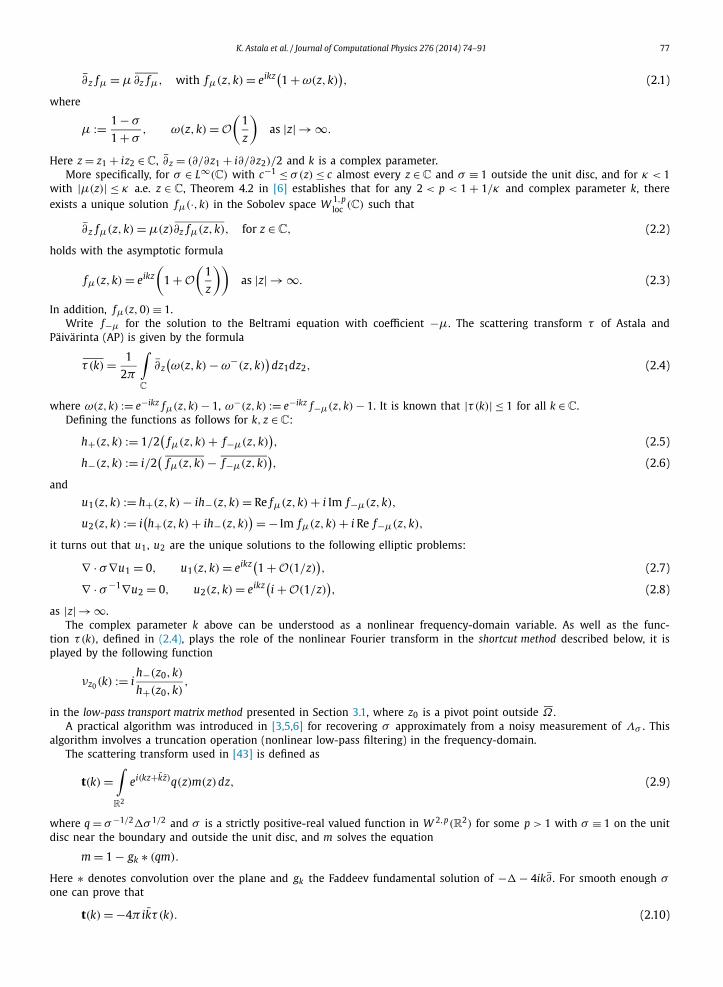
σ2(z) = 2 if |z| < 0.1, 0.2 < |z| < 0.3 or 0.4 < |z| < 0.5 and σ2(z) = 1 otherwise. Fig. 6 shows its profiles.

Computing the scattering transform For conductivity σ2 the scattering transform τ̃11 (with mz = 11) turns out to be very accurate too. Indeed, ̃t10 and ̃t11 corresponding to σ2 are quite similar for |k| small in view of Fig. 7 and the following facts (see notation (4.3)):

84 K. Astala et al. / Journal of Computational Physics 276 (2014) 74–91

Fig. 6. Rotationally symmetric conductivity example σ2. Left: plot of σ2 as a function of z ranging in the unit disc with jump discontinuities along the curves |z| = 0.1, |z| = 0.2, |z| = 0.3, |z| = 0.4, |z| = 0.5. Right: Profile of σ2 as a function of |z| ranging in [0, 1] with jump discontinuities at |z| = 0.1, |z| = 0.2, |z| = 0.3, |z| = 0.4, |z| = 0.5.

Fig. 7. Comparison between ̃t10 and ̃t11 for σ2. Left: Profiles of the real parts of ̃t10 (thin dotted line) and ̃t11 (thick solid line). Right: Profile of the difference Re(̃t10 − t̃11). In both pictures |k| ranges in [0,150] with step h = 0.1. Note that the vertical axis scales are different from Fig. 4.

E[0,20] = 0.4606%, E[20,40] = 3.7474%, E[40,60] = 6.4308%, for σ2,∣∣Re(τ̃11)∣∣ ≤ 1.3653 × 10−7, for σ2.

Solving the D-bar equation Likewise the vector σ̃2(z; mk, R) was computed for R = 5, 10, 15, 20, 25, 30, 35, 40, 50, ..., 150. For R = 5, 10 we took mk = 8, 9 and for the rest of R values we chose mk = 12. All these reconstructions were computed using parallel computation provided by Techila. Fig. 8 shows some of these numerical results. Below we list the errors error2 = max|z|≤1 |Im(σ̃2(z; mk, R))|:

mk 8 8 9 9 12 12 12 12 12 12 12 12 12 12R 5 10 5 10 15 20 25 30 35 40 50 60 70 80error2 × 107 1.56 2.16 1.56 2.17 5.12 5.65 3.97 4.88 6.48 14.1 19.3 14.8 18.4 28.4

mk 12 12 12 12 12 12 12R 90 100 110 120 130 140 150error2 × 107 20.3 20.7 28.8 25.3 24.3 21.8 19.7

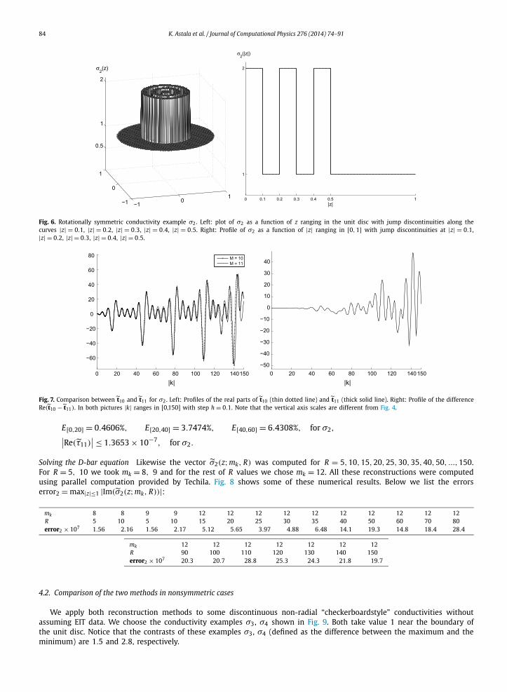
4.2. Comparison of the two methods in nonsymmetric cases

We apply both reconstruction methods to some discontinuous non-radial “checkerboardstyle” conductivities without assuming EIT data. We choose the conductivity examples σ3, σ4 shown in Fig. 9. Both take value 1 near the boundary of the unit disc. Notice that the contrasts of these examples σ3, σ4 (defined as the difference between the maximum and the minimum) are 1.5 and 2.8, respectively.

K. Astala et al. / Journal of Computational Physics 276 (2014) 74–91 85

Fig. 8. Four shortcut method reconstruction examples computed from a scattering transform corresponding to σ2. Each picture shows the real part of the approximate reconstruction (thick line) and the original conductivity σ2 (thin line). In addition, the following information is shown: maximum and minimum values of the real part of the reconstruction, maximum of the absolute value of the imaginary part of the reconstruction (error), taken parameters mk , R , Nx and computation time. Axes scale is the same in the four profiles. These examples were computed using grid computation provided by Techila.

Figs. 12, 13 show the approximate reconstructions for both examples and certain cut-off frequencies R using both meth-ods. The relative errors with sup and l2 norms over the matrix of chosen points in the unit disc are pointed out. We denote such errors as follows:

sup = ‖σ − σ̃‖l∞

‖σ‖l∞· 100%, sqr = ‖σ − σ̃‖l2

‖σ‖l2· 100%,

where σ denotes the actual conductivity and σ̃ the approximate reconstruction.

Low-pass transport matrix method In order to test the low-pass transport matrix method for each conductivity, we obtain the CGO solutions fμ(z0, k), f−μ(z0, k) directly from the known conductivities without simulating EIT data. The point z0 is outside the unit disc and we take the k-grid of 2mk × 2mk equispaced points in the square [−R, R)2 with step hk = R/2mk−1

and cut-off frequencies R ≤ 50. Next, transportation of fμ(z0, k), f−μ(z0, k) to the unit disc and the final reconstruction σ (R)

are performed following the steps described in Section 3.1. To this end, in addition to the k-grid, a grid in the z-variable of 2mz × 2mz equidistributed points in the square [−sz, sz)

2, with step hz = sz/2mz−1, is required.For σ3, σ4 we choose z0 = (−0.88594, −0.88594), z0 = (0, 1.2656), respectively. For σ3 we take mz = 7, mk = 8 and for

σ4 mz = 7, mk = 7. The reconstructions of σ3 could be computed for R ≤ 50 but not for σ4 with R > 20.

Shortcut method Concerning the shortcut method, firstly the approximate scattering transform, denote it by τ SCj for σ j

( j = 3, 4), is computed directly from the known conductivity through the Beltrami equation solver using formula (2.4). The code evaluates the approximation over the points inside the disc of radius R (cut-off frequency) from a k-grid of 2mk × 2mk

equispaced points in the square [−R, R]2. Another z-grid with 2mz × 2mz points in [−sz, sz)2 (sz > 2) is involved here.

86 K. Astala et al. / Journal of Computational Physics 276 (2014) 74–91

Fig. 9. Checkerboard style conductivities σ3, σ4: (a), (c) show the picture for σ3, σ4, resp., using mesh Matlab function. (b), (d) show the values for σ3, σ4, resp., over each tile.

To compute τ SC3 we take R = 50, mk = 8, mz = 10, and for τ SC

4 we choose R = 50, mk = 7, mz = 7. Let us remark that this choice of R enables reconstructions corresponding to cut-off frequencies less than or equal to 50.

Secondly, Figs. 10, 11 show plots of τ SCj and tSC

j , where j = 3, 4 and tSCj is computed from τ SC

j by formula (2.10).Finally, we evaluate the approximate reconstruction by solving the D-bar equation with the truncated scattering trans-

form τ SCj as a coefficient. The reconstructions are computed over the points of the same kind of z-grid as above belonging

to the unit disc with size parameter mz . The code computes the solution to the D-bar equation on every point in the z-grid independently and uses a number of k-grids with size parameter mk and cut-off frequency R .

These reconstructions were evaluated with mz = 7 and some R values with R ≤ 50. In addition, with respect to σ3 we took mk = 9 and for σ4, mk = 7.

Notice that the case R = 50 was correctly computed for both conductivities σ3, σ4 using the shortcut method, but for σ4the highest R-value through the low-pass transport matrix method was R = 20.

4.3. Numerical evidence of the transport matrix efficiency

In addition, further numerical experiments were made aimed at comparing the actual complex geometric optics solution to the Beltrami equation

∂ z fμ(z,k0) = μ(z)∂z fμ(z,k0), for z ∈ Ω, k0 = 1,

and the transported solution f̃μ(z, k0) to the unit disc from fμ(z0, k0) and f−μ(z0, k0) at certain z0 ∈ C \ Ω .Fig. 14 shows some pictures for fμ(z, k0) and f̃μ(z, k0) corresponding to the conductivity example σ4. Here |z| < 1,

k0 ≈ 1 and the pivot point outside the unit disc is z0 ≈ (0, 1.266). To compute f̃μ the transport matrix was generated with a cut-off frequency R = 20 and we took the size parameters as follows: mk = 7, mz = 7, sz = 1.5.

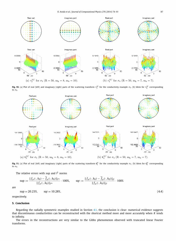
K. Astala et al. / Journal of Computational Physics 276 (2014) 74–91 87

Fig. 10. (a) Plot of real (left) and imaginary (right) parts of the scattering transform τ SC3 for the conductivity example σ3. (b) Idem for τ SC

4 corresponding to σ4.

Fig. 11. (a) Plot of real (left) and imaginary (right) parts of the scattering transform tSC3 for the conductivity example σ3. (b) Idem for tSC

4 corresponding to σ4.

The relative errors with sup and l2 norms

sup := ‖ fμ(·,k0) − f̃μ(·,k0)‖l∞

‖ fμ(·,k0)‖l∞· 100%, sqr := ‖ fμ(·,k0) − f̃μ(·,k0)‖l2

‖ fμ(·,k0)‖l2· 100%

are

sup = 20.23%, sqr = 10.28%, (4.4)

respectively.

5. Conclusion

Regarding the radially symmetric examples studied in Section 4.1, the conclusion is clear: numerical evidence suggests that discontinuous conductivities can be reconstructed with the shortcut method more and more accurately when R tends to infinity.

The errors in the reconstructions are very similar to the Gibbs phenomenon observed with truncated linear Fourier transforms.

88 K. Astala et al. / Journal of Computational Physics 276 (2014) 74–91

Fig. 12. Comparison of reconstructions for σ3 by the low-pass transport matrix method (left) and the shortcut method (right) using different cut-off frequencies R . The chosen point z0 appears in black. The true conductivity is represented at the bottom row.

Fig. 13. Comparison of reconstructions for σ4 by the low-pass transport matrix method (left) and the shortcut method (right) using different cut-off frequencies R . The chosen point z0 appears in black. The true conductivity is represented at the bottom row.

K. Astala et al. / Journal of Computational Physics 276 (2014) 74–91 89

Fig. 14. Comparison of fμ(z, k0) and f̃μ(z, k0) for the conductivity σ4 with R = 20. In the first row we show real and imaginary parts of both functions. In (a) the real part of the actual solution fμ(z, k0) is depicted on the left and the real part of the transported f̃μ(z, k0) on the right (where the point z0

is represented in black). In (b) the same information is showed for the imaginary part of fμ(z, k0) and f̃μ(z, k0). The last row (c) shows the difference f̃μ(z, k0) − fμ(z, k0). The real part is exhibited on the left and the imaginary part on the right. Again, the pivot point z0 appears in black. All the pictures were generated under the same colormap using Matlab.

The numerical study of the nonsymmetric examples comparing both reconstruction types leads us to two observations:

– For these discontinuous conductivity examples, the shortcut method generates considerably better reconstructions than the transport matrix method.

– The approximate solution computed by the transport matrix method is reliable on an area within the unit disc close enough to the selected z0 point outside the unit disc.

Finally, since errors (4.4) are small and plots for both functions fμ(z, k0), f̃μ(z, k0) are similar in view of Fig. 14, we have numerical evidence supporting the fact that the transport matrix method “transports well” and the worse results by the transport matrix method are explained by the final algebraic steps, including numerical differentiation in (3.12), just after the computation of the solutions u(R)

1 (z, k0), u(R)2 (z, k0) in (3.11) through the transport matrix itself.

Acknowledgements

This work was supported by the Finnish Centre of Excellence in Inverse Problems Research 2012–2017 (Academy of Finland CoE-project 250215). In addition, K.A. was supported by Academy of Finland, projects 75166001 and 1134757, and L.P. was supported by European Research Council, Finland, Advanced Grant 267700 InvProb. The third author was also partially supported by Academy of Finland (Decision number 141075) and Ministerio de Ciencia y Tecnología, Spain, grant MTM2011-02568.

Appendix A

This appendix is aimed at presenting two final discussions as follows. On a hand, the noisy scattering transform referred to in Section 3.2 is compared with the free-noise scattering transform computed by solving the Beltrami equation and formula (2.4) for the checkerboard-style conductivity phantom σ3 from Fig. 9. On the other hand, a quantitative discussion on the precision required to the DN map to obtain the accuracy of the scattering transform on the disc of radius 50 is introduced.

Example of noisy scattering transforms For simplicity of notation, let us write τp for the scattering data obtained on the disc centered at the origin of radius 6 by solving the boundary integral equation mentioned in Section 3.1 from a simulated Dirichlet-to-Neumann map, Λp , with p% noise. Additionally, denote by τ the aforementioned free-noise scattering transform on the same disc (denoted by τ SC

3 in Section 4.2).The approximate Dirichlet-to-Neumann map Λp is computed adding p% Gaussian noise to the FEM boundary voltages

(for σ3) as it is explained in Section 5.3 of [20].

90 K. Astala et al. / Journal of Computational Physics 276 (2014) 74–91

Fig. 15. Profiles of the values of E p(r) in (0, 1) with r ∈ (0, 6), for p = 0.1% (black), p = 0.5% (blue), p = 1% (green), p = 5% (red). (For interpretation of the references to color in this figure legend, the reader is referred to the web version of this article.)

The k-grid consists of 2mk × 2mk equispaced points in the square [−6, 6]2 with mk = 7. The scattering data are computed on the 12,851 points of such grid belonging to the disc of radius 6. For the grid in the z-variable used to compute τ , 2mz × 2mz equidistributed points are taken in the square [−sz, sz)

2, with step hz = sz/2mz−1 and sz = 2.3.For different choices of p the following absolute error is computed for r varying over a partition of the interval (0, 6]:

E p(r) := ∥∥χD(0,r)(τ − τp)∥∥

L∞ ,

where χD(0,r) denotes the characteristic function of the disc centered at the origin and radius r.In Fig. 15 the profiles of E p(r) for p = 0.1%, 0.5%, 1%, 5% are shown in black, blue, green and red color, respectively. The

maximum value shown on the vertical axis is 1.

Accuracy of the DN map to compute t(k) on D(0, 50) How many correct significant digits would one need in the DN map for computing the scattering transform t(k) for |k| < 50? It is well-known [1] that there is a logarithmic relation between measurement accuracy and details in conductivity. In other words, EIT is an exponentially ill-posed inverse problem. In terms of scattering transforms, a fixed noise level p% in the EIT measurement leads to, roughly speaking, the computation of t(k) to be stable and accurate in a disc |k| < R(p) and unstable outside that disc. See [34, Fig. 2]. The exponential ill-posedness shows up as a logarithmic dependence of R on p, see [34, Fig. 3]. Improving the measurement accuracy so that the DN matrix entries have one more significant digit increases the stability radius from R to R +Γ with Γ > 0 a fixed real number.

Let us make a crude quantitative estimation based on [34, Fig. 3]. Two significant digits in the DN map corresponds to R = 3 and six significant digits to R = 7. A quick computation shows that achieving the stability radius R = 50 would require 49 correct significant digits in the elements of the DN matrix (and, actually, using a larger matrix with more oscillatory basis functions involved as well).

References

[1] G. Alessandrini, Stable determination of conductivity by boundary measurements, Appl. Anal. 27 (1988) 153–172.[2] K. Astala, T. Iwaniec, G. Martin, Elliptic Partial Differential Equations and Quasiconformal Mappings in the Plane, Princeton Mathematical Series, vol. 48,

Princeton University Press, Princeton, NJ, 2009.[3] K. Astala, J. Mueller, L. Päivärinta, A. Perämäki, S. Siltanen, Direct electrical impedance tomography for nonsmooth conductivities, Inverse Probl. Imaging

5 (2011) 531–549.[4] K. Astala, J. Mueller, L. Päivärinta, S. Siltanen, Numerical computation of complex geometrical optics solutions to the conductivity equation, Appl.

Comput. Harmon. Anal. 29 (2010) 391–403.[5] K. Astala, L. Päivärinta, A boundary integral equation for Calderón’s inverse conductivity problem, in: Proc. 7th Internat. Conference on Harmonic

Analysis, in: Collectanea Mathematica, 2006.[6] K. Astala, L. Päivärinta, Calderón’s inverse conductivity problem in the plane, Ann. Math. 163 (2006) 265–299.[7] R.M. Brown, G. Uhlmann, Uniqueness in the inverse conductivity problem for nonsmooth conductivities in two dimensions, Commun. Partial Differ.

Equ. 22 (1997) 1009–1027.[8] M. Brühl, Explicit characterization of inclusions in electrical impedance tomography, SIAM J. Math. Anal. 32 (2001) 1327–1341.[9] M. Brühl, M. Hanke, Numerical implementation of two non-iterative methods for locating inclusions by impedance tomography, Inverse Probl. 16

(2000) 1029–1042.[10] A.-P. Calderón, On an inverse boundary value problem, in: Seminar on Numerical Analysis and its Applications to Continuum Physics, Rio de Janeiro,

1980, Soc. Brasil. Mat., Rio de Janeiro, 1980, pp. 65–73.[11] P. Caro, A. García, J.M. Reyes, Stability of the Calderón problem for less regular conductivities, J. Differ. Equ. 254 (2013) 469–492.[12] M. Cheney, D. Isaacson, J.C. Newell, Electrical impedance tomography, SIAM Rev. 41 (1999) 85–101.

K. Astala et al. / Journal of Computational Physics 276 (2014) 74–91 91

[13] A. Clop, D. Faraco, A. Ruiz, Stability of Calderón’s inverse conductivity problem in the plane for discontinuous conductivities, Inverse Probl. Imaging 4 (2010) 49–91.

[14] R. Croke, J.L. Mueller, M. Music, P. Perry, S. Siltanen, A. Stahel, The Novikov–Veselov equation: theory and computation, preprint, arXiv:1312.5427, 2013.[15] D. Faraco, K. Rogers, The Sobolev norm of characteristic functions with applications to the Calderón inverse problem, Q. J. Math. 64 (2013) 133–147.[16] A. Friedman, Detection of mines by electric measurements, SIAM J. Appl. Math. 47 (1987) 201–212.[17] B. Gebauer, N. Hyvönen, Factorization method and inclusions of mixed type in an inverse elliptic boundary value problem, Inverse Probl. Imaging 2

(2008) 355–372.[18] B. Haberman, D. Tataru, Uniqueness in Calderón’s problem with Lipschitz conductivities, Duke Math. J. 162 (2013) 497–516.[19] S. Hamilton, C. Herrera, J.L. Mueller, A. Von Herrmann, A direct D-bar reconstruction algorithm for recovering a complex conductivity in 2-D, Arxiv,

preprint, 2012.[20] S. Hamilton, M. Lassas, S. Siltanen, A direct reconstruction method for anisotropic electrical impedance tomography, Inverse Probl. 30 (7) (2014) 075007,

http://dx.doi.org/10.1088/0266-5611/30/7/075007, arXiv:1402.1117.[21] M. Hanke, B. Schappel, The factorization method for electrical impedance tomography in the half-space, SIAM J. Appl. Math. 68 (2008) 907–924.[22] B. Harrach, J.K. Seo, Detecting inclusions in electrical impedance tomography without reference measurements, SIAM J. Appl. Math. 69 (2009)

1662–1681.[23] B. Harrach, M. Ullrich, Monotonicity-based shape reconstruction in electrical impedance tomography, SIAM J. Math. Anal. 45 (2013) 3382–3403.[24] M. Huhtanen, A. Perämäki, Numerical solution of the R-linear Beltrami equation, Math. Comput. 81 (2012) 387–397.[25] N. Hyvönen, Application of the factorization method to the characterization of weak inclusions in electrical impedance tomography, Adv. Appl. Math.

39 (2007) 197–221.[26] T. Ide, H. Isozaki, S. Nakata, S. Siltanen, Local detection of three-dimensional inclusions in electrical impedance tomography, Inverse Probl. 26 (2010)

035001.[27] T. Ide, H. Isozaki, S. Nakata, S. Siltanen, G. Uhlmann, Probing for electrical inclusions with complex spherical waves, Commun. Pure Appl. Math. 60

(2007) 1415–1442.[28] M. Ikehata, S. Siltanen, Numerical method for finding the convex hull of an inclusion in conductivity from boundary measurements, Inverse Probl. 16

(2000) 1043–1052.[29] M. Ikehata, S. Siltanen, Electrical impedance tomography and Mittag–Leffler’s function, Inverse Probl. 20 (2004) 1325–1348.[30] D. Isaacson, J. Mueller, J. Newell, S. Siltanen, Imaging cardiac activity by the D-bar method for electrical impedance tomography, Physiol. Meas. 27

(2006) S43–S50.[31] D. Isaacson, J.L. Mueller, J.C. Newell, S. Siltanen, Reconstructions of chest phantoms by the D-bar method for electrical impedance tomography, IEEE

Trans. Med. Imaging 23 (2004) 821–828.[32] K. Knudsen, A new direct method for reconstructing isotropic conductivities in the plane, Physiol. Meas. 24 (2003) 391–403.[33] K. Knudsen, M. Lassas, J. Mueller, S. Siltanen, D-bar method for electrical impedance tomography with discontinuous conductivities, SIAM J. Appl. Math.

67 (2007) 893.[34] K. Knudsen, M. Lassas, J. Mueller, S. Siltanen, Regularized D-bar method for the inverse conductivity problem, Inverse Probl. Imaging 3 (2009) 599–624.[35] K. Knudsen, J. Mueller, S. Siltanen, Numerical solution method for the dbar-equation in the plane, J. Comput. Phys. 198 (2004) 500–517.[36] K. Knudsen, A. Tamasan, Reconstruction of less regular conductivities in the plane, Commun. Partial Differ. Equ. 29 (2004) 361–381.[37] M. Lassas, J.L. Mueller, S. Siltanen, A. Stahel, The Novikov–Veselov equation and the inverse scattering method: II. Computation, Nonlinearity 25 (2012)

1799–1818.[38] M. Lassas, J.L. Mueller, S. Siltanen, A. Stahel, The Novikov–Veselov equation and the inverse scattering method, Part I: Analysis, Physica D 241 (2012)

1322–1335.[39] A. Lechleiter, N. Hyvönen, H. Hakula, The factorization method applied to the complete electrode model of impedance tomography, SIAM J. Appl. Math.

68 (2008) 1097–1121.[40] J. Mueller, S. Siltanen, Direct reconstructions of conductivities from boundary measurements, SIAM J. Sci. Comput. 24 (2003) 1232–1266.[41] J. Mueller, S. Siltanen, Linear and Nonlinear Inverse Problems with Practical Applications, SIAM, 2012.[42] M. Music, P. Perry, S. Siltanen, Exceptional circles of radial potentials, Inverse Probl. 29 (2013).[43] A.I. Nachman, Global uniqueness for a two-dimensional inverse boundary value problem, Ann. Math. 143 (1996) 71–96.[44] P.A. Perry, Miura maps and inverse scattering for the Novikov–Veselov equation, e-prints, arXiv:1201.2385, 2012.[45] S. Siltanen, J. Mueller, D. Isaacson, An implementation of the reconstruction algorithm of A. Nachman for the 2-D inverse conductivity problem, Inverse

Probl. 16 (2000) 681–699.[46] G. Uhlmann, J.-N. Wang, Reconstructing discontinuities using complex geometrical optics solutions, SIAM J. Appl. Math. 68 (2008) 1026–1044.[47] G. Vainikko, Fast solvers of the Lippmann–Schwinger equation, in: Direct and Inverse Problems of Mathematical Physics, Newark, DE, 1997, in: Int. Soc.

Anal. Appl. Comput., vol. 5, Kluwer Acad. Publ., Dordrecht, 2000, pp. 423–440.