JOURNAL OF Economic Dy namics Control ELSEVIERpublic.econ.duke.edu/~boller/Econ.883/cogley_nason_jedc_95.pdf · JOURNAL OF Economic Dy namics Journal of Economic Dynamics and Control

JOURNAL OF Economic Dy namics

Journal of Economic Dynamics and Control

ELSEVIER & Control

19 (1995) 253-278

Effects of the Hodrick-Prescott filter on trend and difference stationary time series

Implications for business cycle research

Timothy Cogley , *qa James M. Nasonb

‘Research Department. Federal Reserve Bunk of San Fruntisco. San Francisco. C4 94120. IYSA

’ Department of Economics, University of British Colcmhia, Vancower, B.C., Vf T IZI. c’amrdu

(Received April 1993: final version received September 1993)

Abstract

When applied to persistent time series, the Hodrick-Prescott filter can generate business cycle dynamics even if none are present in the original data. Hence the presence of business cycles in HP filtered data does not imply that there are business cycles in the

original data. For example, we show that standard real business cycle models do not generate business cycle dynamics in pre-filtered data and that the business cycles observed in HP filtered data are due to the filter. As another example, we show that under plausible assumptions HP stylized facts are determined primarily by the filter and reveal

little about the dynamics of the underlying data.

I&J% words: Business fluctuations; Time series models; Model evaluation and testing JEL dmsijicutian: E32; C22; C52

1. Introduction

Macroeconomic time series often have an upward drift or trend which makes them nonstationary. Since many statistical procedures assume stationarity, it is

*Corresponding author

We thank Roger Craine, Jon Faust, Andrew Harvey, Stephen LeRoy, Charles Nelson, Adrian

Pagan, Kenneth West, and a referee for helpful comments. Much of this research was done while

Cogley was visiting the Haas School of Business at U.C. Berkeley, and their hospitality is gratefully acknowledged. Opinions expressed in this paper do not necessarily represent the views of the

Federal Reserve Bank of San Francisco or the Federal Reserve System.

0165-1889/95/$07.00 8 1995 Elsevier Science B.V. All rights reserved

SSDI 016518899300781 X

254 T. Cogley, J.M. Nason / Journal of Economic Dynamics and Control I9 (1995) 253-278

often necessary to transform data before beginning analysis. There are a number of familiar transformations, including deterministic detrending, stochastic detrending, and differencing. In recent years, methods for stochastic detrending have received much attention (e.g., Hodrick and Prescott, 1980; Beveridge and Nelson, 1981; Watson, 1986). This paper studies the Hodrick-Prescott (HP) filter, which has become influential in the real business cycle literature. Kydland and Prescott (1982) used this technique in their seminal ‘Time to Build’ paper, and it has been widely adopted by subsequent authors.

The HP filter is a two-sided symmetric moving average filter, and a number of authors have studied its basic properties. Singleton (1988) shows that it operates like a high pass filter when applied to stationary time series.’ King and Rebel0 (1993) show that it can transform series which are integrated of order 4 or less into stationary series. They also characterize a class of unobserved components models for which the HP filter is the optimal Wiener filter, but they suggest that it is an uninteresting class. These authors also give a number of examples which demonstrate that the dynamics of HP filtered data can differ dramatically from the dynamics of detrended or differenced data.

This paper builds on earlier work by distinguishing the HP filter’s effects on trend- and difference-stationary time series (TS and DS, respectively). Many previous results on the HP filter rely on theorems which assume that the original data are stationary. This assumption is problematic, since the filter is typically applied to nonstationary data. We show that Singleton’s result extends in a straightforward manner when the data are TS. In this case, HP filtering is conceptually equivalent to a two-step operation: linearly detrend the data and then apply the HP filter to deviations from trend. Thus the HP filter operates like a high pass filter on deviations from trend.

When the data are DS, the filter does not operate like a high pass filter. In this case, the HP filter is equivalent to a two-step linear filter: difference the data to make them stationary and then smooth the differenced data with an asymmetric moving average filter. The smoothing operation amplifies growth cycles at business cycle frequencies and damps long- and short-run fluctuations. As a consequence, the filter can generate business cycle periodicity and comovement even if none are present in the original data. In this respect, applying the HP filter to an integrated process is similar to detrending a random walk (Nelson and Kang, 1981).’ This has an important practical

‘A stationary time series can be decomposed into orthogonal periodic components. A high pass

filter removes the low frequency or long cycle components and allows the high frequency or short

cycle components to pass through.

‘Nelson and Kang show that a detrended random walk exhibits spurious cycles whose average length is roughly two-thirds the length of the sample. Thus there are important transitory fluctu-

ations in the detrended series even though there are none in the original data.

T. Coglqv, J.M. Nason / Journal of Economic Dynamics and Control 19 (1995) 253-278 255

implication: if an applied researcher is reluctant to detrend a series on account of the Nelson-Kang result, she should also be reluctant to apply the HP filter.

We use these results to study two applications of the HP filter. One is in studies which describe stylized facts about business cycles (e.g., Kydland and Prescott, 1990). The problem with using the HP filter for this purpose is that it is subject to the Nelson-Kang critique. Since the HP filter can generate spurious cycles when applied to integrated processes, it is not clear whether the results should be interpreted as facts or artifacts. We show that if U.S. data are modeled as DS, stylized facts about periodicity and comovement primarily reflect the properties of the implicit smoothing filter and tell us very little about the dynamics of the underlying data.

A second application is in real business cycle (RBC) simulations. Many authors use the HP filter to transform data generated by RBC models. When passed through the HP filter, artificial data display business cycle periodicity and comovement. These fluctuations depend on three factors: impulse dynamics, propagation mechanisms, and the HP filter. We investigate the role the filter plays in generating these dynamics. Using a conventional RBC model, we show that the combination of persistent technology shocks and the HP filter is sufficient to generate business cycles in artificial data. Propagation mechanisms are unnecessary, and in many models they do not play an important role.3

Finally, we consider how HP filtering affects judgments about goodness of fit. The great majority of papers in the RBC literature rely on informal, subjective comparisons of population and sample moments. Such informal judgments are not robust to alternative data transformations. In particular, post-HP filter dynamics often seem to match well even when pre-filter dynamics do not. Thus, on the ‘eyeball metric’, the HP filter can mask important differences between sample and theoretical dynamics. Since results based on informal comparisons are sensitive to HP filtering, it is important to develop methods which are robust. We show how to construct goodness of fit statistics which are invariant to HP filtering, and we apply them to a standard model.

Our discussion is organized as follows. Section 2 describes the HP filter and analyzes its effects on TS and DS processes. Section 3 considers the problem of interpreting stylized facts, and Section 4 examines the filter’s role in generating periodicity and comovement in RBC models. Section 5 dis- cusses the problem of evaluating goodness of fit in filtered data. Section 6 concludes.

3Cogley and Nason (1992) provide an extensive analysis of the role of propagation mechanisms in

RBC models.

256 T. Cogley, J.M. Nason / Journal of Economic Dynamics and Control 19 (1995) 2S3-278

2. Effects on trend- and difference-stationary time series

The HP filter decomposes a time series into cyclical and growth components: y(t) E g(t) + c(t), where y(t) is the natural logarithm of the observed series, g(t) is the growth component, and c(t) is the cyclical component. To identify the two components, Hodrick and Prescott minimize the variance of c(t) subject to a penalty for variation in the second difference of the g(t),”

y$ I tzz, [y(t) - sw + Pff, CsO + 1) - 3?(t) + SO - 1)12i;

where p controls the smoothness of the growth component.’ The solution to this problem is a linear time-invariant filter which maps y(t) into c(t). The HP cyclical component can be written as c(t) = H(L)(l - L)4y(t), where H(L) equals

(lp1’/L2)[1 - 2Re(p)L + Ip12L2]-‘[1 - 2Re(p)L-’ + ip12L-2]-1.

The parameter l/p is a stable root of the lag polynomial [,L-’ L2 + (1 - L)4] = 0, Re(p) denotes the real part p, and lpl2 is its mod-square.6

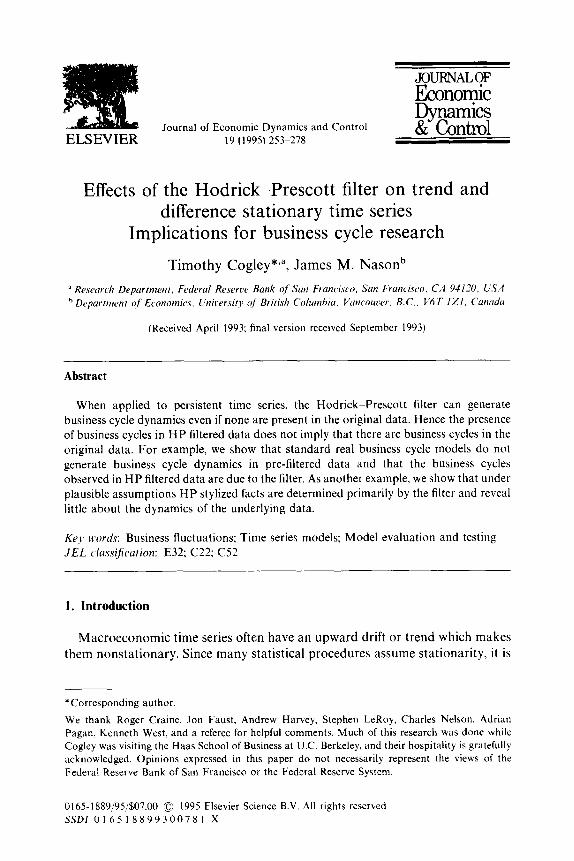
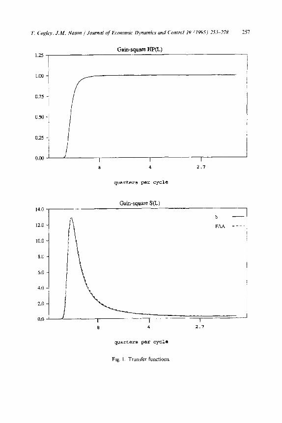
The proper interpretation of the filter’s effects depends on the nature of original data. Suppose that y(t) is stationary and mixing.7 In this case, y(t) has a Cramer representation, which means that it can be decomposed into orthogonal periodic components. When the HP filter operates on a stationary series, the spectra for the input and output series satisfy _&cc(o) = IHP(o)12&(w), where f&(w) is the spectrum for c(t), fYY(o) is the spectrum for y(t), and ]HP(w)12 is the squared gain of the filter (1 - L)4H(L). The gain indicates how the filter affects the amplitude of the periodic component of y(t) at frequency w. If [HP(w)) > 1, then the filter increases the amplitude of the frequency o component of y(t). Similarly, if [HP(w)1 < 1, the filter decreases the amplitude of the frequency o component. The function IHP(o)l’ is shown in the top panel of Fig. 1 (taken from Singleton, 1988). When applied to stationary series, the HP

4Thev actually formulate a related finite horizon problem, the solution to which is a time-varying

filter.VIn the finite horizon case, the moments of dg(t) and c(t) depend on time and hence are

nonstationary. The solution to the infinite horizon problem is a time-invariant filter which generates

covariance stationary processes for dg(r) and c(t) for the input processes studied in this paper. Since the filters are otherwise quite similar, we prefer to analyze the version which generates stationary

output processes.

5As p increases, g(r) becomes smoother. In the limit, g(t) becomes a linear deterministic trend. When

applied to quarterly data, p is almost always set equal to 1600.

‘That is, IpI2 = pp, where p is the complex conjugate of p.

‘The latter condition ensures that the data have a short span of dependence.

T. Co&y, J.M. Nason f Journal of Economic Dynamics and Control 19 11995) 253-278 251

Gain-square HP(L)

0.25 1

0.00 - I I I a 4 2.7

quarters per cycle

Gain-square S(L) 14.0

s -

12.0 - FM _---

IO.0 -

8.0 -

I

h.0 -

4.0 -

2.0 -

0.0 I I I I 8 4 2.7

quarters pet cycle

Fig. 1. Transfer functions.

258 T. Cogley, J.M. Nason / Journal of Economic Dynamics and Control 19 (1995) 253-278

filter operates like a high pass filter, damping fluctuations which last longer than eight years per cycle (in quarterly data) and passing shorter cycles without change.

This result relies fundamentally on the Cramer representation of a stationary time series. Since a stationary series can be decomposed into orthogonal periodic components, it is meaningful to analyze how the filter operates on its periodic components. This result has limited practical value, however, because the HP filter is typically applied to nonstationary time series, which do not have Cramer representations (Priestley, 1988). It is not meaningful to analyze the periodic components of y(t) when y(t) does not have a periodic decomposition!

An alternative approach is useful when the data are nonstationary. Decom- pose the filter into two operations, one which renders y(t) stationary by an appropriate transformation and another which operates on the resulting stationary series. Then it is possible to determine the filter’s effect on the stationary component of y(t) by analyzing the properties of the second operation. We use this approach to analyze the HP filter’s effect on TS and DS processes. We also consider the special case of a near unit root, TS process.*

2.1. Trend-stationary processes

Suppose that y(t) is TS: y(t) = c1 + /It + z(t), where z(t) is stationary and mixing. Applying the HP filter term by term yields

c(t) = H(L)(l - L)“z(t).

Applying the HP filter to a TS process is conceptually equivalent to a two-step operation: linearly detrend y(t) to make it stationary and then apply the HP filter to the deviations from trend, z(r). Since z(t) is stationary and mixing, Singleton’s characterization extends in a straightforward manner. The HP filter works like a high pass filter on deviations from trend.

2.2. Diference-stationary processes

Now suppose that y(t) is DS: dy(t) = cx + u(r), where u(t) is stationary and mixing. In this case, the HP filter operates like a two-step linear filter. Difference y(t) to make it stationary, and then smooth dy(t) with an asymmetric moving average filter:

s Harvey and Jaeger (1993) use this approach to compare the HP filter with the optimal Wiener filter

for an unobserved components model of trend and cycle.

T. Cogley, J.M. Nason / Journal of Economic Dynamics and Control 19 (1995) 253-278 259

where

S(L) = H(L)(l - L)3.

Since dy(t) is stationary and mixing, we can apply the usual theorems on linear filters to analyze the properties of S(L). The solid line in the bottom pane1 of Fig. 1 shows its squared gain.’

S(L) is not a high pass filter. When applied to quarterly data, it amplifies growth cycles at business cycle frequencies and damps long- and short-run components. Its gain has a maximum at 7.6 years per cycle and increases the variance of this frequency component by a factor of 13. S(L) also amplifies neighboring frequencies. For example, it increases the variance of growth cycles lasting between 3.2 and 13 years by more than a factor of 4.

To illustrate the filter’s effect on DS processes, we conduct a variant of the Nelson-Kang (1981) experiment. Consider the effect of applying the HP filter to a pair of random walks. Specifically, assume that dyl(t) and dy,(t) are white noise variates which are correlated at lag zero but uncorrelated at all other leads and lags. The spectra1 density matrix for the vector c(t) isf&) = ) S(w)(‘fdd(w), wheref,,(w) is the spectra1 density matrix for the vector dy(t).” The elements of fdd(o) are constants, sofcc(o) inherits the spectral shape of S(t).

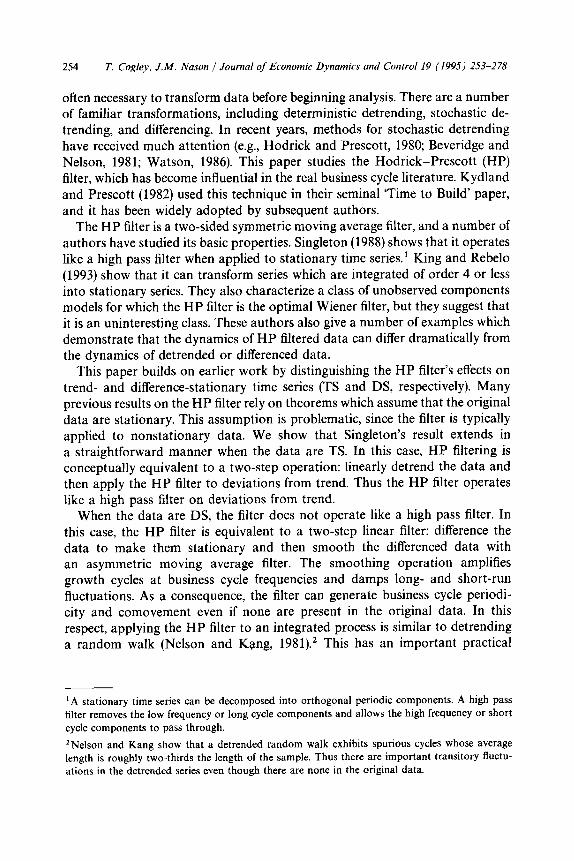
Since the power spectrum for an HP filtered random walk is proportional to (S(w)j’, it has a peak at 7.6 years per cycle. Hence there is business cycle periodicity in the elements of c(t) even though the elements of y(t) are random walks. The cross-spectrum is also proportional to 1 S(w)\‘, so the elements of c(t) also display comovements over business cycle horizons.’ 1

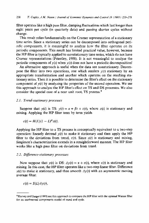
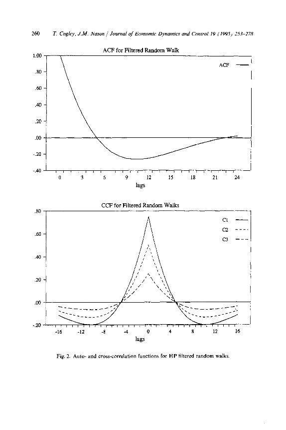
Fig. 2 translates this information into time domain. The top panel shows the autocorrelation function for an HP filtered random walk. It has strong positive autocorrelation at short horizons and negative autocorrelation at long horizons. This pattern is similar to the autocorrelation function for a detrended random walk. The bottom pane1 shows cross-correlation functions for HP filtered random walks. The contemporaneous correlations between the pre-filtered series are set equal to 2, f, and a, respectively. The cross-correlation function has

‘This is drawn for p = 1600. As p increases, the peak becomes larger, narrower, and moves to lower

frequencies. The dotted line in Fig. 1 will be discussed below.

“Let d,(w) denote the frequency o component of the vector time series y(t). The spectral density

matrix is proportional to the covariance matrix for the complex random vector d,(o).

‘I We do not claim that S(L) always generates business cycle comovement in DS processes. For

example, if dy,(t) and dy,(t) are uncorrelated at all leads and lags, c,(t) and c,(t) are also uncorrelated at all leads and lags. But this exception is irrelevant to macroeconomists, since dynamic

economic models rarely generate series which are uncorrelated at all leads and lags. Our example is

relevant, since the assumed cross-correlations are similar to comovements which arise in many RBC

models.


1.00

\

ACF for Filtered Random Walk

ACF -

20 -

.60 -

.20- \

40 -

-40 I I 1 / I / I , I I1 / I I / I I I / I I I I I

0 3 6 9 12 15 18 21 24

lags

30 , CCF for Filtered Random Walks

1 Cl -

c2 ___. .60 -

c3 ---

.40 -

-16 -12 -8 -4 0 4 8 12 16

lags

Fig. 2. Auto- and cross-correlation functions for HP filtered random walks.

T. Cogley, J.M. Nason / Journal qf Economic Dynamics and Control 19 11995) 2S3-27X 261

the same shape as the autocorrelation function, with the scale depending on the

size of the contemporaneous correlation between dyi(t) and dyz(t). One might think that HP filtered dynamics reflect business cycle periodicity

and comovement. In the short run, there is positive dependence over time and across series, and there is trend reversion and error correction in the long run.

However, in this example, the business cycle dynamics of c(t) are artifacts of the filter. This shows that HP filtered data can exhibit periodicity and comovement over business cycle horizons even if none are present in the input series. Hence the presence of business cycle dynamics in c(t) does not imply business cycle dynamics in y(t).

2.3. A special case: Near unit root TS processes

If macroeconomic time series are modeled as TS processes, deviations from trend have large autoregressive roots. As one might expect, the effect

of the HP filter on near unit root processes is much like its effect on unit root processes. To see why, let 5(t) = (1 - $L)z(t), where 4 is the largest

autoregressive root of z(t); b, is close to but less than one. The HP cyclical component is c(t) = {(l - L)/(l - 4L)}S(L)z”(t). The term in brackets is a near common factor whose gain has a narrow trough near frequency zero and is close to one at all other frequencies. Since its gain is close to one at high and medium frequencies, it has little influence on the high and medium frequency dynamics of c(t). Further, its influence near frequency zero is largely

negated by the low frequency damping effect of S(L). Thus c(t) is well approximated by S(L)I(t). Since 5(t) is quasi-differenced z(t), it typically has a relatively flat spectrum. Therefore the spectrum for c(t) has roughly the same shape as

lS(@12. As an example, consider the technology shock process used in many RBC

models: A(t) = it + (1 - 0.95L))’ E(L). The dotted line in the bottom panel of

Fig. 1 graphs the spectrum for HP filtered A(t). It is nearly indistinguishable from /So’.

3. Interpreting stylized facts about business cycles

The HP filter is sometimes used to describe stylized facts about business cycles (e.g., Kydland and Prescott, 1990). The problem with using the HP filter for this purpose is that it is subject to the Nelson-Kang critique. Since the HP filter can generate spurious cycles in DS processes, it is not clear whether the results should be regarded as facts or artifacts. Hence the interpretation of stylized facts depends on assumptions about the nature of the input series. King and Rebel0 (1993) consider how to interpret HP stylized facts when the data are assumed to

262 T. Cogley. J.M. Nason / Journal of Economic Dynamics and Control 19 (1995) 253-278

Y 4.0

Spectrum for ,,

3.5 3.0

:: , I

2.5 I: 2.0 1.5 I.0 .5 .O m

; ; I ' : : ' '\

2.00 Co-spectrum C,Y

1.75 ::

1.50 I: 1.25 1.00 .75

.50 r

; ; 'I I :

: ',

8 4 2.7

-.os ’ I

Spectrum for C 1.25, ,,

t7 4 2.7

quarters per cycle

80

70 60 50

40 30

20 10 0

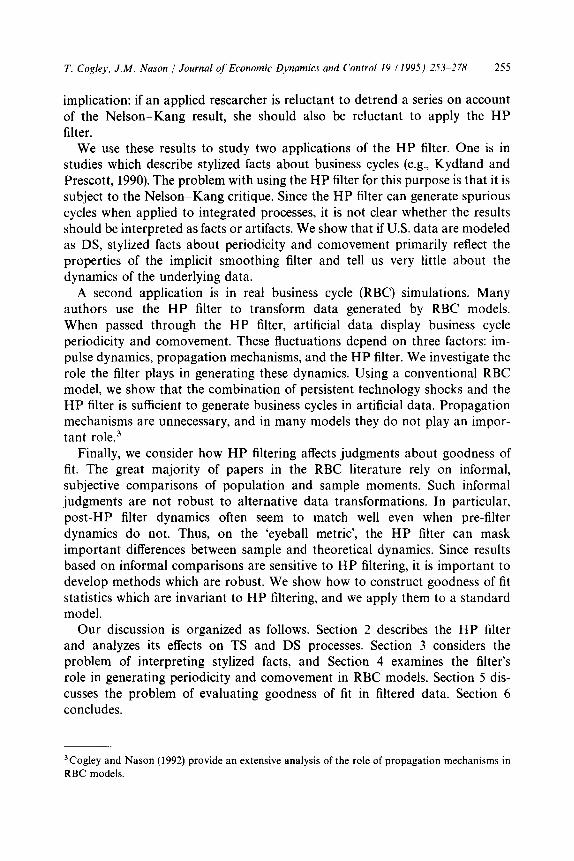
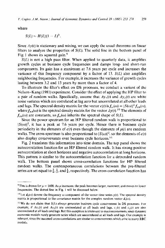
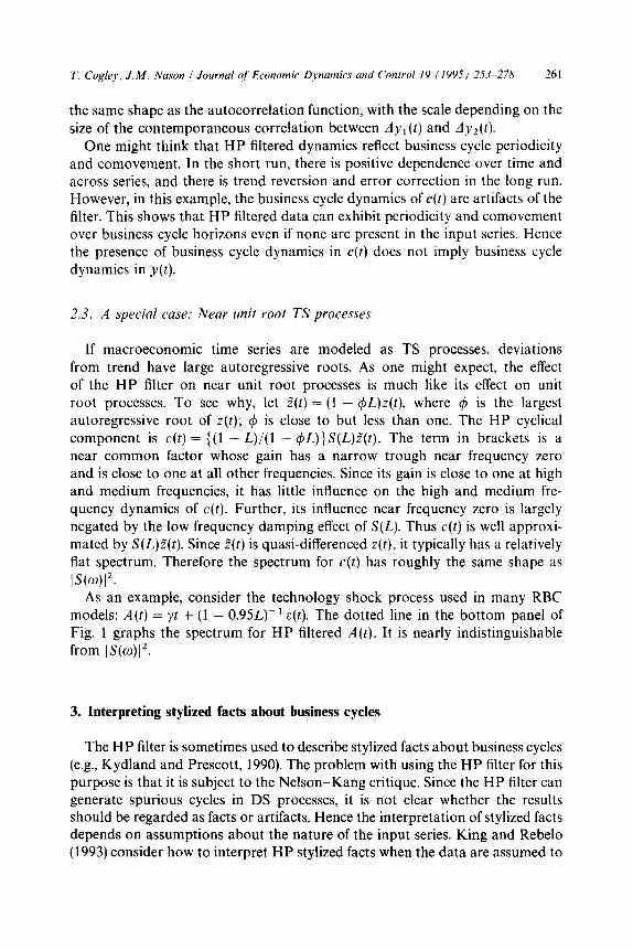
Fig. 3. Spectral density matrices, before and after filtering.

be TS.r2 This section complements their work by considering the interpretation of stylized facts when the data are modeled as DS.

Although it is customary to summarize periodicity and comovement by reporting auto- and cross-correlations, it is more convenient for our purpose to examine spectral density matrices. The spectral density matrix contains the same information as auto- and cross-correlations and makes it easier to interpret the effects of filtering.

Fig. 3 shows estimated spectral density matrices for quarterly U.S. real GNP, real personal consumption expenditures, and real gross private domestic fixed

“Briefly, since TS representations of macroeconomic time series have near unit roots, most of the

variation is due to low frequency components. Since the HP filter damps low frequency fluctuations in detrended data, it reduces the amplitude and average length of cycles.

T. Cogley, J.M. Nason / Journal qf Economic Dynamics and Conrrol 19 11995) 253-278 263

investment. All three series are measured in per capita units, and the sample period is 1954-1991. The graphs on the diagonal are power spectra, the graphs below the diagonal are co-spectra (the real part of cross-spectra), and the graphs above the diagonal are quadrature spectra (the imaginary part of cross-spectra). The solid lines are the elements offdd(m), and the dotted lines are the elements offeJW).l 3

This figure shows that HP cyclical components have their own ‘typical spectral shape’ which is essentially the same as the IS(o) Experimentation with other variables and sample periods verifies that this is robust. To interpret this, decompose the dynamics of c(t) into two parts: the dynamics of dy(t) and the effects of S(L). Pre- and post-smoothing spectral density matrices are related by the equation jJo) = lS(o)[* &(o). S’ mce the elements of fdd(w) are flat relative to IS(o) the elements off,,(w) inherit the shape of IS(w)l’. Hence the smoothing filter is the primary determinant of the dynamics of c(t). Growth dynamics have only a secondary influence. Since the spectra for HP filtered data mainly reflect the shape of IS(o)12, auto- and cross-correlations of HP filtered data reveal more about the properties of the smoothing operation than about the properties of dy(t). In the DS case, HP stylized facts are determined primarily by the filter.

The literature on HP stylized facts suffers from the same problem as Kuznets’ (1961) work on long swings in growth. In looking for evidence of long swings, Kuznets employed a filter which was designed to remove business cycles from the data, and he found evidence of 20-year cycles in the filtered data. Adelman (1965) and Howrey (1968) later analyzed the properties of the Kuznets filter and found that it would generate 20-year cycles even if the original data were white noise or white noise around a deterministic trend. Thus the presence of 20-year cycles in Kuznets filtered data does not imply that there are 20-year cycles in the original data. Long swings might simply be an artifact of filtering. Similarly, since the HP filter can generate spurious business cycles, the presence of business cycles in HP filtered data does not imply that there are important transitory fluctuations in the original data.

4. Sources of periodicity and comovement in RBC models

Business cycle theorists are interested in periodicity, comovement, and relative volatility (e.g., Lucas, 1987; Prescott, 1986). In this section, we focus on periodicity and comovement.14 In the RBC literature, periodicity is usually

13The spectral density matrix for dy(t) was estimated by smoothing the matrix periodogram using a Bartlett window. This was multiplied by IS(o)l’ to obtain the spectral density matrix for c(r).

14King and Rebel0 (1993) show that the HP filter alters relative volatilities, increasing the relative

volatility of investment and hours and decreasing that of consumption and real wages.

264 T. Cogley. JAI. Nason / Journal of Economic Dynamics and Control 19 (1995) 253-278

measured by the autocorrelation function of output, and comovements are summarized by cross-correlations between output and variables such as consumption, investment, and hours. Since most macroeconomic data are nonstationary, some transformation is needed in order to make second moments finite. Following Kydland and Prescott (1982) many authors use the HP filter to induce stationarity.

When artificial data are passed through the HP filter, they display periodicity and comovement over business cycle horizons. These fluctuations depend on three factors: the exogenous impulse dynamics which drive the model, the endogenous propagation mechanisms which spread shocks over time, and the HP filter. This section investigates the role the HP filter plays in generating periodicity and comovement. Using a conventional RBC model, we show that the combination of persistent technology shocks plus the HP filter is sufficient to generate business cycle periodicity and comovement. Propagation mechanisms are unnecessary, and, in many cases, do not play an important role.

We study TS and DS representations of the Christiano-Eichenbaum (CE) (1992) model. Its dynamics are essentially the same as those of many other RBC models, so the results reported below apply to many other models.‘5

4.1. The d@erence-stationary model

The CE model is driven by technology and government spending shocks. In the DS version, the natural logarithm of technology follows a random walk with drift, and the natural logarithm of government spending evolves as a stationary process around the technology shock. The natural logarithms of output, consumption, and investment inherit the unit root in the technology shock, while the natural logarithm of hours worked follows a stationary process. Since output, consumption, and investment are DS, we compare HP filtering with first differencing. Hours are stationary, so no preliminary transformation is needed.

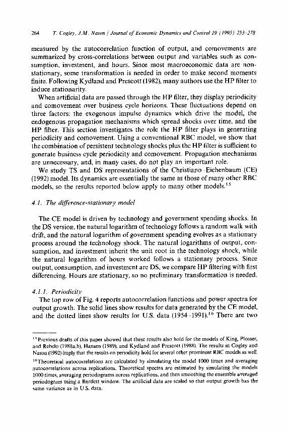
4. I .I. Periodicity The top row of Fig. 4 reports autocorrelation functions and power spectra for

output growth. The solid lines show results for data generated by the CE model, and the dotted lines show results for U.S. data (1954-1991).i6 There are two

“Previous drafts of this paper showed that these results also hold for the models of King, Plosser,

and Rebel0 (1988a,b), Hansen (1989). and Kydland and Prescott (1988). The results in Cogley and

Nason (1992) imply that the results on periodicity hold for several other prominent RBC models as well.

“jTheoretica1 autocorrelations are calculated by simulating the model 1000 times and averaging

autocorrelations across replications. Theoretical spectra are estimated by simulating the models

1000 times, averaging periodograms across replications, and then smoothing the ensemble averaged

periodogram using a Bartlett window. The artificial data are scaled so that output growth has the

same variance as in U.S. data.


.40 Pre-smoothing ACF

.32- “, L

.24- ‘, 1

.16- : ,

.08- :

I .oo---$- I’.

\_’ ’ ,“.,__- .

\ ,’

Pre-smoothing spectra .00060 -

;\ _ .00050

I ‘1 ‘4

: , 1 ‘1 .00040 - \

3 .; t,

s10030 - , ’ \ --T

I .00020 ,

\ 1-x ‘I _, , \ ‘I

.OOOlO- ,,’ ..I- \I

. -.08’,,,,,,,,.,,,,,..,.,, J .OOOUI) d 2 7 12 17

8 4 2.7

96, Post-smoothing ACF Post-smoothing spectra

I .0025 , ,,

.0021)

.0015

.OOlO

.0005

2 7 12 17 a b 2:7

lags quarters per cycle

Fig. 4. Autocorrelations and power spectra, before and after filtering (DS model).

interesting facts about artificial output dynamics. The first is that the model does not generate business cycle periodicity. Output growth is very weakly autocorrelated at all lags, and its spectrum is quite flat. Fluctuations at business cycle frequencies are no more important than fluctuations at any other frequency.

Second, the periodicity of output growth is determined primarily by shock dynamics, with little contribution from the model’s endogenous propagation mechanisms. Output growth is well approximated by a white noise variate, and total factor productivity growth is also white noise. Since output dynamics are essentially the same as impulse dynamics, it follows that the model’s internal propagation mechanisms are weak.

The bottom row of Fig. 4 shows the effects of HP filtering on autocorrelations and power spectra. Since output growth is nearly white noise in the CE model, the spectrum for HP filtered output inherits the shape of IS(o)12. Transforming 1 S(w) I2 into time domain produces positive autocorrelation for four quarters, followed by negative dependence for several years. In this model, the source of

266 T. Cogley. J.M. Nason 1 Journal of Economic Dynamics and Control 19 (1995) 253-278

business cycle periodicity in HP filtered data is the HP filter! An RBC model can exhibit business cycle periodicity in HP filtered data even if it does not generate business cycle periodicity in output growth.

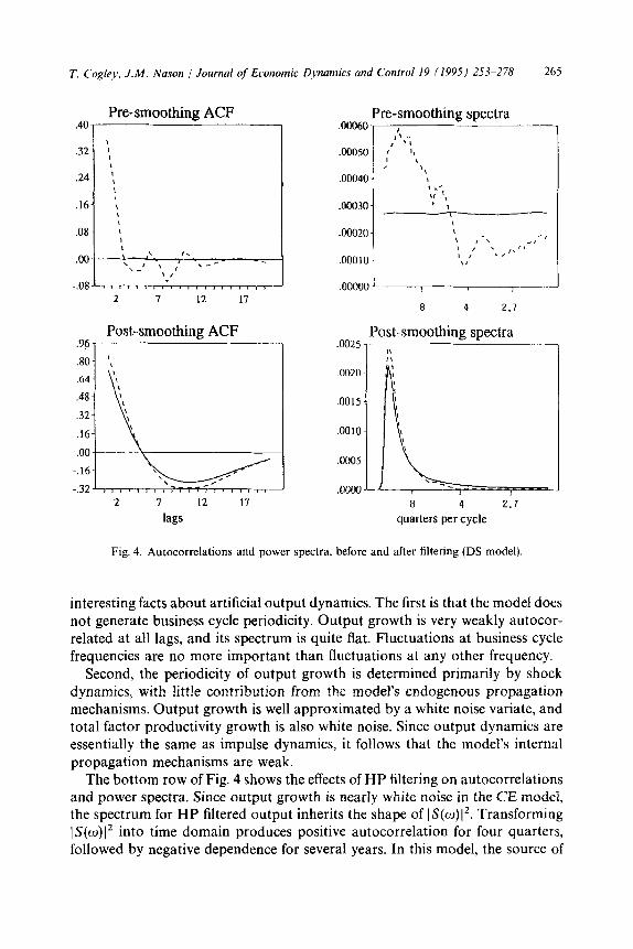
4.1.2. Comovement Figs. 5a and 5b report cross-correlation functions and cross-spectra, before

and after filtering. The solid lines show results for artificial data, and the dotted lines are for U.S. data. The first two rows of Fig. 5a report comovements of consumption and investment growth with output growth. In the CE model, consumption and investment growth are very highly correlated with output growth at lag zero (0.91 for consumption and 0.99 for investment) and nearly uncorrelated at nonzero leads and lags. In frequency domain, the theoretical cross-spectra are flat everywhere except near frequency zero.

CCF 1.00

dc,dy

.75

.50

.25

.OO

-.25 -9 0 9

CCF 1.00

di,dy

.I5

.50

.25

.oo

-.25 -9 0 9

CCF h,dy

-9 0 9

lags

a 4 2.7

Co-spectra h,dy LO,, 1.0

Quad-spectra h,dy

:::L___J :::: a 4 2.7

quarters per cycle

a 4 2.7

quarters per cycle

Fig. Sa. Pre-filter comovements (DS model).

T. Cogley, J.M. Nason 1 Journal qf Economic Dyzamics and Control 19 (1995) 253-278 261

-9 0 9

.80

.60

.40

.20

.oo

-.20

-.40

-9 0 9

CCF ch,cy

1 ‘\ 1 \ If \

,,.,a:

,’ I’ \ \

‘._,’ ‘_

-9 0 9

lags

2.0 Co-spectra cc,cy

-..

6 1.5 ;:

1.0 ( : ’

.5 ‘8,

.O I:.,_

-.5d 8 4 2.7

2,0 Quad-spectra cc,cy

1.5

1.0

.5

;_

I’\ .o ’

-.5’- I

15.0 Co-spectra ci,cy

12.5 10.0

,? , (

1.5 : : 5.0 ; ‘, 215 ‘\_

.O -2.5 -5.0 I--

8 4 2.7

8 4 2.7

Quad-spectra ci,cy

8 4 2.7 8 4 2.7

quarters per cycle quarters per cycle

Fig. 5b. Post-filter comovements (DS model)

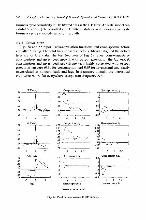
The CE cross-correlation functions for consumption and investment growth conform closely to those considered in the Nelson-Kang experiment in Section 2.2. From that example, we know that S(L) spreads contemporaneous correlations over periods of several years, thus giving an impression of covariation over business cycle horizons. Since the pre-filter cross-spectra are relatively flat (except near frequency zero), the post-filter cross-spectra inherit the shape of lS(w)12. Taking the inverse Fourier transform of lSo)(’ produces the bell-shaped cross-correlation functions shown in Fig. 5b. An RBC model can exhibit business cycle comovements in HP filtered data even when pre-filter comovements are almost entirely contemporaneous.

Cross-correlations between output growth and hours exhibit a different pattern, and this is shown in the third row of Fig. 5a. The CE model generates weak negative correlation at low order leads, a contemporaneous correlation of roughly 0.3, and slowly decaying correlations at low order lags. In this case, the model does generate dynamic covariation in pre-filtered data. After the data are passed through the HP filter, however, the cross-correlation function exhibits


Pre-filter ACF

.oo -

-.20 L 2 I 12 17

1.W Post-filter ACF

.75

2 7 12 17 lags

Pre-filter spectra .HJ‘Io - \

I .0035- ’

8 4 2.7

Post-filter spectra .0040 -

.0035- j

.01)30 ;/ .0025- : .ou20 : 1 .0015

.OOlO

.0005~

.oowJ

8 4 2.7 quarlers per cycle

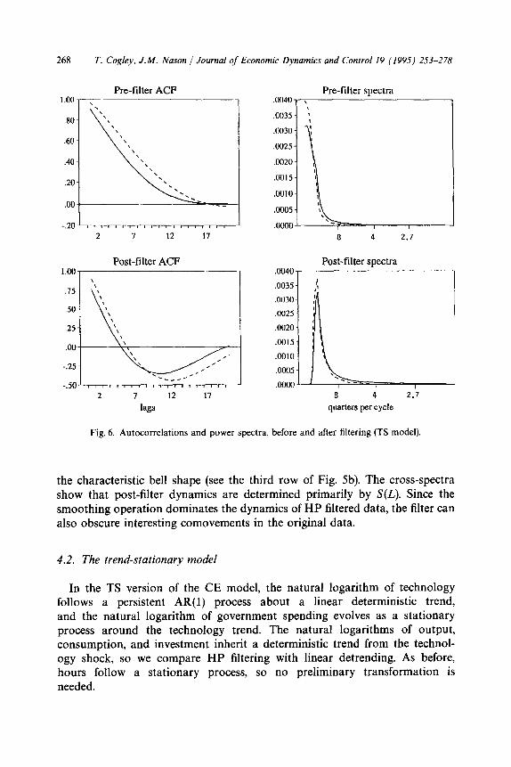
Fig. 6. Autocorrelations and power spectra, before and after filtering (TS model).

the characteristic bell shape (see the third row of Fig. 5b). The cross-spectra show that post-filter dynamics are determined primarily by S(L). Since the smoothing operation dominates the dynamics of HP filtered data, the filter can also obscure interesting comovements in the original data.

4.2. The trend-stationary model

In the TS version of the CE model, the natural logarithm of technology follows a persistent AR(l) process about a linear deterministic trend, and the natural logarithm of government spending evolves as a stationary process around the technology trend. The natural logarithms of output, consumption, and investment inherit a deterministic trend from the technology shock, so we compare HP filtering with linear detrending. As before, hours follow a stationary process, so no preliminary transformation is needed.

T. Cogley, J.M. Nason / Journal of Economic Dynamics and Control I9 11995) 253-278 269

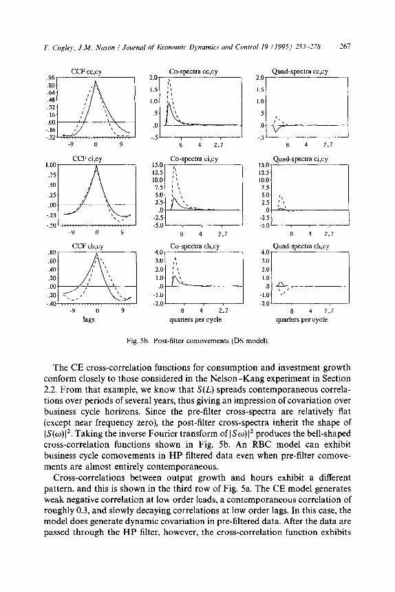
4.2.1. Periodicity The top row of Fig. 6 reports autocorrelation functions and power spectra for

detrended output. The solid lines are theoretical moments, and the dotted lines are sample moments.’ ’ In the TS CE model, one can show that output is well approximated by an AR(l) process about trend with an AR coefficient of approximately 0.95 (e.g., Cogley and Nason, 1993). Since the technology shock is also a persistent AR(l) process about trend, we again observe that output dynamics are essentially the same as impulse dynamics. Output periodicity is determined primarily by impulse dynamics with little contribution from propagation mechanisms.

The bottom row of Fig. 6 reports autocorrelations and power spectra for HP filtered data. Since output has a near unit root in this model, the results of Section 2.3 apply. The spectrum for HP filtered output inherits the shape of IS(w)12. Transforming IS(w)l’ into time domain produces the usual autocorrelation pattern. The combination of a near unit root in technology and the HP filter is sufficient to generate business cycle periodicity in HP filtered output.

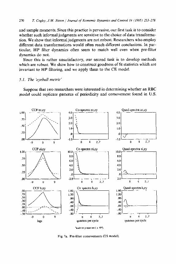
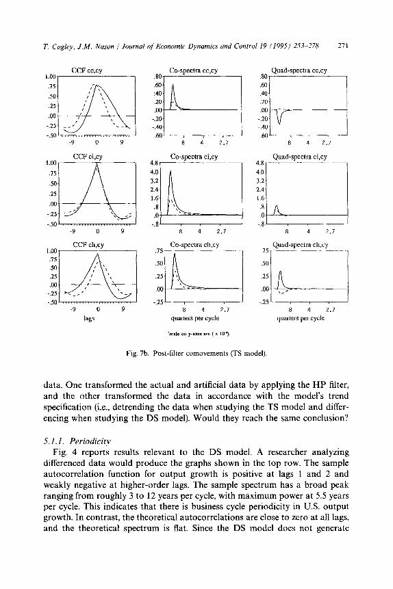
4.2.2. Comovement Figs. 7a and 7b report cross-correlation functions and cross-spectra for the TS

model. The solid lines show results for artificial data, and the dotted lines are for U.S. data. Fig. 7a reports comovements of detrended consumption, detrended investment, and hours with detrended output. In the CE model, all three variables are highly correlated with output at lag zero, and cross-correlations decay slowly at low-order leads and lags. In frequency domain, the co-spectra have peaks near zero, and the quad-spectra indicate that there are fairly substantial phase shifts in consumption and hours and a minor phase shift in investment.

Fig. 7b reports comovements for HP filtered data. After filtering, the cross- spectra inherit the shape of lS(w)12. Transforming into time domain generates the characteristic bell-shaped cross-correlation function. HP filtered data have their own typical spectra1 shape, and this pattern comes from the filter S(L).

5. Evaluating goodness of fit

This section considers the problem of evaluating goodness of fit in HP filtered data. In the RBC literature, most authors do not report forma1 test statistics. Instead, it is common to rely on informal, subjective comparisons of population

“Theoretical moments are calculated by simulating the model 1000 times and averaging across

replications. The artificial data are scaled so that detrended output has the same variance as in

sample.


and sample moments. Since this practice is pervasive, our first task is to consider whether such informal judgments are sensitive to the choice of data transformation. We show that informal judgments are not robust. Researchers who employ different data transformations would often reach different conclusions. In particular, HP filter dynamics often seem to match well even when pre-filter dynamics do not.

Since this is rather unsatisfactory, our second task is to develop methods which are robust. We show how to construct goodness of fit statistics which are invariant to HP filtering, and we apply them to the CE model.

5.1. The ‘eyeball metric’

Suppose that two researchers were interested in determining whether an RBC model could replicate patterns of periodicity and comovement found in U.S.

1.00 CCF zc,zy

I.

‘, .I5

2’ ,~,/ ‘.._

;/\\

‘.

so *’

.25

1.00, CCF zi,zy

,

.I5 ,” ’ ‘\

so K ,J’ ‘\ \

.25 ,I’ ‘__.

.oo -9 0 9

4.0 Co-spectra zc,zy

3.0 ‘1,

2.0 :

El

L 1.0

.O

-l.OL IO.0 Co-spectra zi,zy

8.0

6.0 ‘\

4.0 :

2.0 :

.O

-2.0 L 8 4 2.7

1.60

1.20 .80 .40 .OO

-.40 -.80

Co-spectra h,zy

:I!EI

:

:

8 4 2.7 quoters per cycle

his an y-axes NC ( x 109.

4.0 Quad-spectra zc,zy

3.0

2.0

1.0

.O

-1.0 r-- a 4 2.7

lo,o Quad-spectra zi,zy

8.0

6.0

4.0

2.0

.o ’

-2.0 L! a 4 2.7

::~~, Quad-speclra lwy

.80

.40

.oo _. -.40 -.80 k

a 4 2.7

quarters per cycle

Fig. 7a. Pre-filter comovements (TS model).


I.001 CCF cc,cy

1 .75

SO .25

.oo

-.25

-SO -9 0 Y

_. -9 a 9

-9 0 9

lags

4.81 Co-spectra ci,cy

I

8] I

_I -.25- 8 4 2.7

quarters per cycle

,80 Quad-spectra cc.cy

.60

.40

.20

.oo -

-.20 -.40

-.60 LiEI 8 4 2.7

4.8 Quad-spectra ci,cy

4.0

3.2

2.4 1.6

.8

.O I, -.8 J I

8 4 2.7

Quad-speclrd ch,cy .15,~

_J -.25- 8 4 2.7

quarters per cycle

Fig. 7b. Post-filter comovements (TS model).

data. One transformed the actual and artificial data by applying the HP filter, and the other transformed the data in accordance with the model’s trend specification (i.e., detrending the data when studying the TS model and differencing when studying the DS model). Would they reach the same conclusion?

5.1.1. Periodicity Fig. 4 reports results relevant to the DS model. A researcher analyzing

differenced data would produce the graphs shown in the top row. The sample autocorrelation function for output growth is positive at lags 1 and 2 and weakly negative at higher-order lags. The sample spectrum has a broad peak ranging from roughly 3 to 12 years per cycle, with maximum power at 5.5 years per cycle. This indicates that there is business cycle periodicity in U.S. output growth. In contrast, the theoretical autocorrelations are close to zero at all lags, and the theoretical spectrum is flat. Since the DS model does not generate

272 T. Cogley. J.M. Nason / Journal of Economic Dynamics and Control I9 (1995) 253-278

business cycle periodicity, a researcher analyzing these results would probably conclude that the model fails to replicate the dynamics of U.S. output growth.

A researcher analyzing HP filtered data would produce the graphs shown in the bottom row of Fig. 4. This researcher would observe that actual and artificial data are both positively autocorrelated at low-order lags and negatively autocorrelated at higher-order lags. In frequency domain, the sample and theoretical spectra both have large peaks at roughly 7.5 years per cycle. Since there appears to be an excellent match between sample and theoretical moments, this researcher would be likely to conclude that the model matches sample output dynamics quite well.

Fig. 6 reports results relevant to the TS model. A researcher analyzing detrended data would produce the graphs shown in the top row. Both actual and artificial data are well approximated by persistent autoregressive processes. However, while the artificial data are well approximated by an AR(l) process, U.S. data are well approximated by an AR(2) process with two positive real roots.18 Thus the model generates less persistence than observed in sample. In other words, the model generates too little low frequency power.

A researcher studying HP filtered data would produce the graphs shown in the bottom row. Since the HP filter eliminates low frequency information in TS processes, the low frequency discrepancy observed in detrended data vanishes. A researcher analyzing HP filtered data would probably conclude that the model matches sample output dynamics quite well.

Researchers who employ different data transformations are likely to reach different conclusions about periodicity. Researchers who analyze HP filtered data would be likely to draw favorable conclusions, while those who analyze differenced or detrended data would not. The reason why actual and artificial HP filtered data appear to have common dynamic properties is that they inherit common dynamic factors from the filter. After filtering, actual and artificial spectra look alike because they both display the spectral shape of (S(CO)/~. Autocorrelation functions for HP filtered data look alike because they display the characteristic HP pattern, which is the inverse Fourier transform of (S(CO)[~. Thus, on the ‘eyeball metric’, the periodicity of HP filtered output appears to match well even though pre-filter measures of periodicity do not.

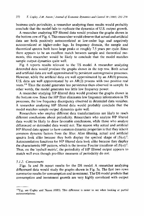
5.1.2. Comovement Figs. 5a and 5b report results for the DS model. A researcher analyzing

differenced data would study the graphs shown in Fig. 5a. The first two rows summarize results for consumption and investment. The DS model predicts that consumption and investment growth are very highly correlated with output

lsE.g., see Cogley and Nason (1993). This difference is easier to see when looking at partial autocorrelations.


growth at lag zero and are very weakly correlated at other leads and lags. In contrast, observed comovements are spread out over several quarters. Sample cross-correlations are lower than predicted at lag zero (0.54 for consumption and 0.8 for investment) and larger than predicted at low-order leads and lags (roughly 0.25 to 0.35). A researcher analyzing differenced data might have doubts about the nearly perfect contemporaneous relation between these variables.

A researcher analyzing HP filtered data would study the graphs shown in the first two rows of Fig. 5b. In this case, the cross-correlations for consumption and investment appear to match quite well. In particular, they have the same bell shape. Thus a researcher analyzing HP filtered data would be more likely to come to a favorable conclusion about the model’s ability to replicate the sample comovements of consumption and investment with output.

The frequency domain graphs show that the bell shape pattern comes from S(L). Before filtering, the cross-spectra are flat relative to S(L). Therefore, when actual and artificial data are passed through S(L), they inherit its spectral shape (Fig. 5b). Transforming IS(o)J’ into time domain produces bell-shaped cross- correlation functions.

Comovements between output and hours are summarized in the third row of Figs. 5a and 5b. Before filtering, the theoretical cross-correlation function has modest negative correlation at low-order leads, a peak of roughly 0.3 at lag 0, and slowly decaying correlations at low-order lags. The sample cross-correlation function has a similar shape, but the contemporaneous correlation is close to zero, and the peak occurs at lags 5 through 7. A researcher analyzing differenced data would note a significant discrepancy between sample and theoretical lead/lag relations. In U.S. data, an increase in output growth is associated with an increase in hours, but this occurs with a lag of 5 to 7 quarters. In the CE model, hours respond contemporaneously.

After filtering, the sample and theoretical cross correlation functions have the characteristic bell shape, with peaks at lags 1 and 0, respectively. A researcher analyzing HP filtered data would be likely to conclude that the model generates the right qualitative comovements but has a relatively minor discrepancy in lead/lag relations.

Figs. 7a and 7b report results for the TS model. The first two rows summarize comovements of consumption and investment with output. Investment/output comovements match well both before and after filtering. Consumption/output comovements seem to match fairly well in a qualitative sense, but there appears to be rather large quantitative discrepancies. In this case, researchers analyzing detrended and HP filtered data would be likely to reach the same conclusions.

The third row reports results for output and hours. Before filtering, the match between sample and theoretical cross-correlations is quite poor. In particular, the predicted correlations between hours and detrended output are much too high. On the other hand, after filtering, the match is much improved. A

274 T. Co&y. J.M. Nason 1 Journal of Economic Dynamics and Control 19 (1995) 253-278

researcher analyzing unfiltered data would be likely to conclude that the model’s implications for hours/output comovements are grossly inconsistent with the data, while a researcher analyzing HP filtered data would be likely to conclude that the model produces a reasonable qualitative match.

5.2. Filter-invariant goodness of jit statistics The results of the previous section highlight the desirability of developing

goodness of fit measures which are invariant to HP filtering. This section constructs invariant spectral goodness of fit statistics. The basic idea is to work with ratios of sample and theoretical spectra. The HP filter multiplies numerator and denominator by the same number, so these ratios are invariant to HP filtering. r9 We investigate the model’s implications for periodicity by computing statistics based on power spectra. We investigate comovement implications by computing statistics based on coherence.20

5.2.1 Periodicity Let R=(O) = Z~(W)/~(O), where IT(m) denotes the sample periodogram and

f(w) denotes the population, model generated spectrum for pre-filtered data. ‘Pre-filtered’ refers to detrended data when studying TS models, and it refers to differenced data when studying DS models. Let U,(o) be proportional to the partial sums of Rr(m): Ur(2rcj/T) = (27c/T)C{= 1 Rr(27ci/T). The variable U,(o) is invariant to HP filtering, since the numerator and denominator of all the elements in the sum are both multiplied by the squared gain of the filter:

where G(o) = IHP(w)12 in the TS case and G(o) = [S(W)[~ in the DS case. Since U,(o) is invariant to HP filtering, any statistic based on U,(o) is also invariant.

Under the hypothesis that the data are drawn from a population governed by f(o), U,(o) converges to a uniform distribution function. Thus goodness of fit

19Watson’s (1993) approach is similar, but his overall goodness of fit statistic is not invariant to

linear filtering, and its statistical properties are unknown.

Z°Coherence is the frequency domain analog to correlation, and it is defined as

If~~(~)12/fil(~)f22(~), wherefI 1(w) and f ( ) 22 w are the power spectra for series 1 and 2 andf,,(o)

is the cross-spectrum.

T. Cogley. J.M. Nason / Journal of Economic Dynamics and Control 19 (1995) 2.53-278 215

Table 1

HP filter-invariant goodness of fit tests

TS model

KS CVM

DS model

KS CVM

(1) Periodicity of output 1.03 0.52 2.44 2.45

(0.239) (0.036) (1.3E-05) (O.OOQ)

(2) Coherence with output

(C>Y) 1.29 0.81 1.12 0.64

(O.OOQ) (0.000) (0.000) (0.000)

(i, Y) 0.53 0.14 0.50 0.13

(0.000) (O.OOQ (0.000) (0.000)

(h* Y) 0.89 0.29 1.16 0.51

(0.000) (0.000) (O.ooo) (0.000)

This table reports Kolmogorov-Smirnov and Cramer-von Mises statistics for TS and DS versions

of the Christiano-Eichenbaum (1992) model. Asymptotic probability values arc shown in paren-

theses.

statistics for uniform distributions can be applied to U,(w). For example, these include the Kolmogorov-Smirnov and Cramer-von Mises statistics:

KS = max l&(r)l,

s 1

CVM = B%z) &, 0

where

B&) = (,/%/27r)[U,(nr) - r&(n)] and 0 I t I 1.

Dzhaparidze (1986) shows that these statistics converge to functionals of a Brownian bridge, and their limiting distributions are tabulated in Shorack and Wellner (1987).

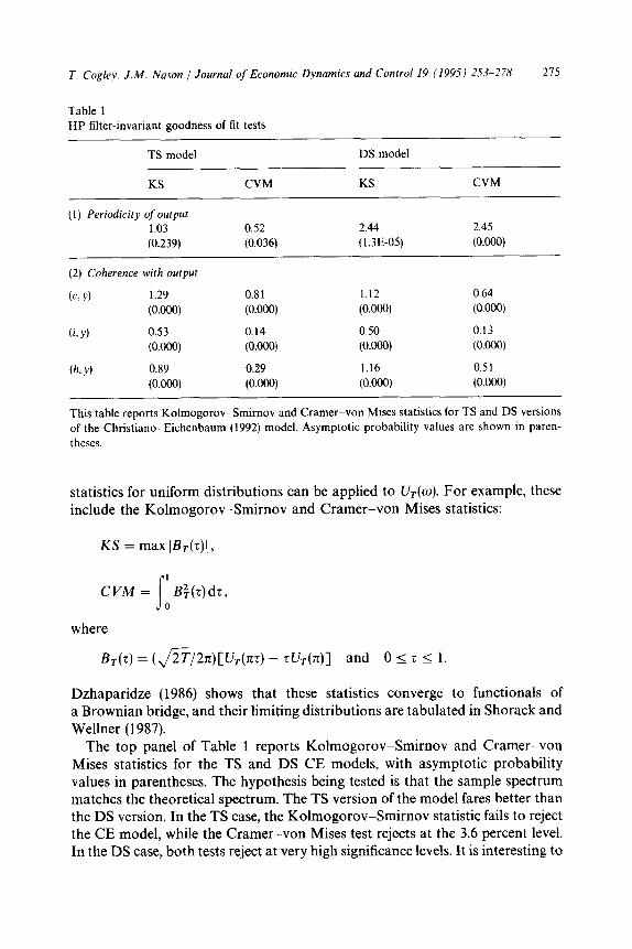
The top pane1 of Table 1 reports Kolmogorov-Smirnov and Cramer-von Mises statistics for the TS and DS CE models, with asymptotic probability values in parentheses. The hypothesis being tested is that the sample spectrum matches the theoretical spectrum. The TS version of the mode1 fares better than the DS version. In the TS case, the Kolmogorov-Smirnov statistic fails to reject the CE model, while the Cramer-von Mises test rejects at the 3.6 percent level. In the DS case, both tests reject at very high significance levels. It is interesting to


note that these results appear to be consistent with informal comparisons based on inspection of detrended and differenced data, but contradict informal judgments based on inspection of HP filtered data.

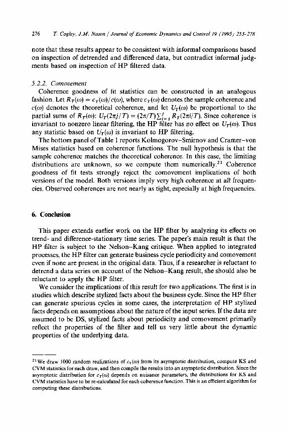
5.2.2. Comovement Coherence goodness of fit statistics can be constructed in an analogous

fashion. Let R~(w) = cr(o)/c(o), where c*(w) denotes the sample coherence and c(o) denotes the theoretical coherence, and let U,(o) be proportional to the partial sums of R,(w): Ur(27rj/ T) = (2x/T)C{= 1 RT(27ci/T). Since coherence is invariant to nonzero linear filtering, the HP filter has no effect on U,(w). Thus any statistic based on U,(o) is invariant to HP filtering.

The bottom panel of Table 1 reports Kolmogorov-Smirnov and Cramer-von Mises statistics based on coherence functions. The null hypothesis is that the sample coherence matches the theoretical coherence. In this case, the limiting distributions are unknown, so we compute them numerically.” Coherence goodness of fit tests strongly reject the comovement implications of both versions of the model. Both versions imply very high coherence at all frequencies. Observed coherences are not nearly as tight, especially at high frequencies.

6. Conclusion

This paper extends earlier work on the HP filter by analyzing its effects on trend- and difference-stationary time series. The paper’s main result is that the HP filter is subject to the Nelson-Kang critique. When applied to integrated processes, the HP filter can generate business cycle periodicity and comovement even if none are present in the original data. Thus, if a researcher is reluctant to detrend a data series on account of the Nelson-Kang result, she should also be reluctant to apply the HP filter.

We consider the implications of this result for two applications. The first is in studies which describe stylized facts about the business cycle. Since the HP filter can generate spurious cycles in some cases, the interpretation of HP stylized facts depends on assumptions about the nature of the input series. If the data are assumed to be DS, stylized facts about periodicity and comovement primarily reflect the properties of the filter and tell us very little about the dynamic properties of the underlying data.

*r We draw 1000 random realizations of cr(w) from its asymptotic distribution, compute KS and

CVM statistics for each draw, and then compile the results into an asymptotic distribution. Since the asymptotic distribution for cr(o) depends on nuisance parameters, the distributions for KS and

CVM statistics have to be re-calculated for each coherence function. This is an efficient algorithm for

computing these distributions.

i”. Cogley, J.M. Nason / Journal of Economir Dynamics and Control 19 (1995) 253-278 211

A second application is in RBC simulations. When artificial data are passed through the HP filter, they exhibit business cycle periodicity and comovement. We inquire into the source of these fluctuations. We show that RBC models can exhibit business cycle dynamics in HP filtered data even if they do not generate business cycle dynamics in pre-filtered data. The combination of a unit root or near unit root in technology and the HP filter is sufficient to generate business cycle dynamics. Propagation mechanisms are unnecessary, and in many RBC models they do not play an important role.

Finally, we consider the problem of evaluating a model’s goodness of fit. In the RBC literature, it is common to rely on informal judgments based on inspection of sample and theoretical moments. Conclusions based on informal comparisons are sensitive to the choice of data transformation. Researchers who analyse HP filtered are often likely to reach different conclusions from researchers who analyze differenced or detrended data. Since actual and artificial data inherit common dynamic factors when they are passed through the filter, HP filtered dynamics can appear to match well even if pre-filter dynamics do not. We show how to circumvent this problem by computing filter-invariant goodness of fit statistics.

References

Adelman, I., 1965, Long cycles: Fact or artifact?, American Economic Review 55, 444-463.

Beveridge, S. and CR. Nelson, 1981, A new approach to decomposition of economic time series into

permanent and transitory components with particular attention to measurement of the business

cycle, Journal of Monetary Economics 7, 15 1-174.

Christiano, L.J. and M. Eichenbaum, 1992, Current real business cycle theories and aggregate labor

market fluctuations, American Economic Review 82, 430-450.

Cogley, T. and J.M. Nason, 1992, Do real business cycle models pass the NelsonPlosser test?,

Mimeo. (Federal Reserve Bank of San Francisco, CA).

Cogley, T. and J.M. Nason, 1993, Impulse dynamics and propagation mechanisms in a real business

cycle model, Economics Letters 43, 7778 1,

Dzhaparidze, K., 1986, Parameter estimation and hypothesis testing in the spectral analysis of

stationary time series (Springer-Verlag, New York, NY).

Hansen, G.D., 1989, Technical progress and aggregate fluctuations, Department of Economics

working paper no. 546 (University of California, Los Angeles, CA).

Harvey, A.C. and A. Jaeger, 1993, Detrending, stylized facts, and the business cycle, Journal of

Applied Econometrics 8, 231-247.

Hodrick, R. and E.C. Prescott, 1980, Post-war U.S. business cycles: An empirical investigation.

Mimeo. (Carnegie-Mellon University, Pittsburgh, PA).

Howrey, E.P., 1968. A spectrum analysis of the long-swing hypothesis, International Economic

Review 9, 228-260.

King, R.G. and S.T. Rebelo, 1993, Low frequency filtering and real business cycles, Journal of Economics Dynamics and Control 17, 2077232.

King, R.G., Cf. Plosser, and S.T. Rebelo, 1988a, Production, growth, and business cycles I: The basic neoclassical model, Journal of Monetary Economics 21, 1955232.

278 T. Cogley. J.M. Nason / Journal of Economic Dynamics and Control 19 (I995) 253-278

King, R.G., C.I. Plosser, and ST. Rebelo, 1988b, Production, growth, and business cycles II: New

directions, Journal of Monetary Economics 21, 309-342.

Kuznets, S.S., 1961, Capital in the American economy: Its formation and financing (National Bureau

of Economic Research, New York, NY).

Kydland, F.E. and E.C. Prescott, 1982, Time to build and aggregate fluctuations, Econometrica 50,

1345-1370.

Kydland, F.E. and E.C. Prescott, 1988, The workweek of capital and its cyclical implications,

Journal of Monetary Economics 21, 343-360.

Kydland, F.E. and E.C. Prescott, 1990, Business cycles: Real facts and a monetary myth, Federal

Reserve Bank of Minneapolis Quarterly Review 14, 3-18.

Lucas, R.E., 1987, Models of business cycles (Basil Blackwell, Oxford).

Nelson, C.R. and H. Kang, 1981, Spurious periodicity in inappropriately detrended time series,

Econometrica 49, 741-751.

Priestley, M.B., 1988, Non-linear and non-stationary time series analysis (Academic Press, New

York, NY).

Prescott, E.C., 1986, Theory ahead of business cycle measurement, Carnegie-Rochester Conference

Series on Public Policy, 1 l-66.

Shorack, G.R. and J.A. Wellner, 1987, Empirical processes with applications to statistics (Wiley,

New York, NY).

Singleton, K.J., 1988, Econometric issues in the analysis of equilibrium business cycle models,

Journal of Monetary Economics 21, 361-368.

Watson, M.W., 1986, Univariate detrending methods with stochastic trends, Journal of Monetary

Economics 18,49-76.

Watson, M.W., 1993, Measures of fit for calibrated models, Journal of Political Economy 101,

1011-1041.

Documents

JOURNAL OF Economic Dy namics Control ELSEVIERpublic.econ.duke.edu/~boller/Econ.883/cogley_nason_jedc_95.pdf · JOURNAL OF Economic Dy namics Journal of Economic Dynamics and Control