Journal of the Meteorological Society of Japan, Vol. 78

Journal of the Meteorological Society of Japan, Vol. 78, No. 3, pp. 289-298, 2000 289

NOTES AND CORRESPONDENCE

Comparative Study of Vertical Motions in the Global Atmosphere

Evaluated by Various Kinematic Schemes

By H. L. Tanaka

Institute of Geoscience, University of Tsukuba, Tsukuba, Japan

and

Akiyo Yatagai

National Space Development Agency of Japan, Earth Observation Research Center, Tokyo, Japan

(Manuscript received 28 May 1999, in revised form 1 March 2000)

Abstract

Large-scale vertical motions estimated by various classical kinematic methods are compared with those of NCEP-NCAR and ECMWF reanalyses. The classical kinematic methods include the central difference

method, plane fitting method, and spectral method. In addition, a normal mode method is proposed in this study as a new approach to the computation of the vertical motion. In this method, the erroneous high frequency divergence is controlled by filtering the higher order gravity modes while the low-frequency Rossby modes are retained.

According to the result, ECMWF reanalysis contains large amount of small-scale eddies, whereas the NCEP-NCAR reanalysis is smoother, reflecting the different spectral truncations. The normal model method provides a reasonable distribution of vertical motion, and the problem in the spectral method over

the complex terrain is solved by this method. It is demonstrated that the normal mode method may be useful for the diagnostic studies of the general circulation of the atmosphere.

1. Introduction

Vertical motion is the key variable for any diag-nostic study in the general circulation, especially for energy and water budgets and various kinds of mate-rial transports in the 3-D atmosphere (e.g., Newell et al. 1972; Kung 1988). Except for some point-wise observations by wind profilers (e.g., Sato 1994; Muschinski et al. 1999), vertical motion is not an ob-servable quantity in a global network. Therefore, we must evaluate it diagnostically from observed hori-zontal wind data. The vertical p-velocity, w, was estimated earlier in the 1960's by an omega equa-tion, assuming an inviscid and adiabatic flow (e.g., Tomatsu 1979). The vertical motion so obtained

provides a general view of ascending and descend-ing motions around the synoptic eddies within the quasi-geostrophic framework. However, it is obvi-ous that such an omega should not be used for the study of heat and energy budgets since the adiabatic and inviscid flow has been assumed from the begin-ning. For this reason, we need to calculate it by integrating a mass continuity equation with respect to the vertical coordinate although this kinematic estimate suffers from errors contained in the obser-vation. Various schemes of the kinematic estimate for the vertical motion using the continuity equation are designed in the 1970's to reduce an observational error contained in the divergence field (e.g., O'Brien 1970; Kung 1972). The recent advancement in the 4-D data assimi-

lation technique seems to have solved such a prob-lem in the classical vertical velocity estimation (see Daley 1991). The vertical motion provided by the

Corresponding author: Hiroshi L. Tanaka, Insti-tute of Geoscience, University of Tsukuba, 1-1-1 Tennoudai, Tsukuba 305-8571, Japan. E-mail: [email protected]

2000, Meteorological Society of Japan

290 Journal of the Meteorological Society of Japan Vol. 78, No. 3

assimilation cycle is kinematically consistent, at least, within the model atmosphere. However, it is often the case that the vertical motion is not avail-able in public for the un-initialyzed global analysis data. We thus need to calculate it by some method for the study of energy and water budgets. Yet, there is no universal and established method to com-pute the vertical motion from the data. The purpose of this study is to compare the ver-

tical motions evaluated by some classical kinematic methods in the global atmosphere. The schemes to be compared include a central difference method, plane fitting method, and spherical harmonic expan-sion method. In addition, a normal mode expansion method is proposed in this study as an extension of the spherical harmonic expansion method to the 3-D spectral domain (see Tanaka and Kung 1988). The characteristics of the vertical motion evaluated by the 3-D normal mode method are argued and compared with those obtained by the other meth-ods. The results are further compared with reanal-yses provided by National Center for Environmen-tal Prediction and National Center for Atmospheric Research (NCEP-NCAR) and European Center for Medium Range Weather Forecasts (ECMWF).

2. Data and method

The data used in this study are twice daily (0000 and 1200 GMT) NCEP-NCAR reanalyses. The data contain horizontal winds v=(u, v), vertical p-velocity w, temperature T, and geopotential, de-fined at every 2.5 longitude by 2.5 latitude grid point over 17 mandatory vertical levels from 1000 to 10hPa. Since w is provided both in the NCEP-NCAR and ECMWF reanalyses, the results com-puted in this study are compared with those w in the reanalyses to find to what extent these values agree with each other. The vertical p-velocity, w, is evaluated from hori-zontal divergence, Vv, in the pressure coordinate by integrating the continuity equation with respect to pressure.

p Vv+aw=0-w=-.

nVvdp.ap(1)

Here, the boundary condition should be w=0 at the limit of p-0.

In the following, we present a finite difference method, plane fitting method, and spectral method for evaluating the divergence in (1). Then, the di-vergence is integrated with respect to the vertical

from the top to bottom of the atmosphere using

the boundary condition. It has been, however, inte-

grated conventionally from the bottom to top since the stratospheric data contains a large observational

error in divergence. The poor quality of the upper

air divergence spoils the whole column of the vertical

motion.

When we integrate it from the bottom to top, we need first to get the surface w under a proper assumption. The resulting contradiction at the top boundary is often adjusted by O'Brine's (1970) quadratic correction. Luo and Yanai (1983) used the objectively analyzed surface winds to calculate the orographically forced uplift at the surface, and the continuity equation is integrated from the bottom to top. The vertical motion so obtained is used for the heat budget analysis over the Tibetan plateau. Unfortunately, this method generates an enormous amount of error over the complex terrain, such as Tibettern Plateau and Antarctic, if we use the to-pography without smoothing. Some additional care is needed to avoid the problem in the mountain-ous region. A tendency of geopotential at 1000hPa surface is used by Tanaka and Milkovich (1990) for evaluating the surface w for the heat budget over Alaska. We found it useful for a situation of negli-gible horizontal wind under the strong temperature inversion. In this study, surface w is computed af-ter Tanaka and Milkovich (1990) using time series of the geopotential data. Finally in this study, a normal mode method is

proposed as a new approach for the computation of the vertical motion, where the atmospheric variables are expanded in 3-D normal model functions. The divergence is integrated analytically from the top to bottom of the atmosphere as desired. The erroneous high frequency divergence is eliminated by filtering the gravity modes while the low-frequency Rossby modes are retained. It will be shown that the prob-lem in the mountainous region is reduced in this method.

2.1 Central difference method In this scheme, the horizontal divergence in (1)

is approximated by a standard central difference method on the finite grid system:

u(+LA)-u(-a)Vv=2 acos8L

V(e+oe)-V(e-oe) +2 a cos BOB (2)

where A and 8 are longitude and latitude, V=V cos 8, and a is the radius of the earth. In this method, the divergence is evaluated by the small difference in the wind speed. Unfortunately, this scheme contains large error in small scales since the observed wind has, at least, 10% of error. The divergence sometimes contains more than 100 per-cent of error because divergent wind is one order of magnitude smaller than rotational wind in mid-latitudes by the geostrophy. For example, when two adjacent tonal winds are 10 and 11ms-1, the di-vergence becomes 1/a cos 8La. If the wind contains 1m/s of observational error, which is about 10% of the wind speed, the error in divergence becomes at

June 2000 H.L. Tanaka and A. Yatagai 291

most 2/a cos oL which appears to be 200% error for divergence. For this reason, the simple difference scheme is danger to use unless some additional care is taken.

2.2 Plane fitting method This method is aimed to remove such an erroneous

divergence in small scales by fitting wind data near the origin onto a plane using a lease square method (see Kung 1972).

u(A,o)=uo+Aa+Bo,

V(A,o)=Vo+Ca+DO,

Vv=A+D a cos o'

(3)

where V=v cos o and the regression coefficients A,

B, C, D are evaluated from a set of gridded data

using the standard multiple regression code. For

the square gridded analysis data, the surrounding

8 points may be adequate to fit a plane. The de-viations from the plane are considered mostly as

an observational error. The divergence tends to be

smoother if the number of the data points increases.

This method has been widely used since it is appli-

cable for randomly distributed observation stations.

The optimal number of the data points for the fitting is determined empirically considering the purpose of

the study. The result of the energy budget would,

however, depend highly on the choice of the fitting

grid number.

2.3 Spectral method

Since the fundamental idea of the successful plane

fitting method is a filtering of divergence in small

scales, it is straightforward to apply the method for

the global data by a spectral expansion technique

in spherical harmonics. Here, the divergence 6 is

expanded in spherical harmonics, and synthesized

over the wavenumbers approximately a half of the

Nyquist wavenumber.

▽・v-δ-Σ Σ δmnpmn(μ)eimλ,

m 1 1 imUm m Vm m bn m 2 a1 -2 Pn a1-2 Hn

(4)

where urn and V m are zonal Fourier expansion co-efficients of u cos 9 and v cos 9, A and o are longitude and latitude, Pn (u) is the associated Legendre func-tions as a function of 1u=sin9m and n are zonal and total wavenumbers, Pn X12=2n+1 is the norm of Pm, and Hn(u)=(1-u2)a is the deriva-tive of The analytical expression is available for H(u). The divergence 6 is evaluated from in-tegration of the observed wind rather than a dif-ferentiation of the wind. If we synthesized over all

wavenumbers, the method would have no advantage for the purpose of evaluating meaningful w. In this study, truncation is set at T-42 considering the grid size of 2.5 longitude by 2.5 latitude.

2.4 Normal mode method The spectral method expands the data in the

spherical harmonics, but the finite difference method is utilized in the vertical. An alternative method is to apply the spectral method even in the vertical.

In this study, we have developed a new spectral method to calculate w by expanding the state vari-ables in 3-D normal mode functions:

U(w,e,p,t)=i:Ewnlm(t)XmHnlm(a,o,p),

whim (t)=<IJ, Xm1Hnim>, (5)

where U=(Cu,v,o')T is the state variable vector of horizontal wind velocity and geopotential perturba-tion from the global mean as functions of longitude A, latitude 9, pressure p and time t. The expansion basis function Hnlm is a tensor product of vertical structure functions Gm and Hough harmonics (see Kasahara 1984). The 3-D spectral expansion coef-ficient wnlm, has triple subscripts of zonal, merid-ional, and vertical wavenumbers, respectively. The dimensional factor matrix Xm=diag(c, cm, c,)contains scale parameters cm=ghm involving the gravity g and the separation constant of the equiva-lent depth hm. The equations in (5) construct a pair of Fourier transforms in the 3-D spectral domain with a proper inner product <w,z> which satisfies an orthonormal condition for Ilnlm

Once the expansion coefficient wnlm is obtained, the vertical motion w may be calculated by the syn-thesis of the modes, corresponding to the inverse transform:

CmpG dGm inaCJ=2Swnlm2nlmZnlmeR'y dp (6)

where 1 is the angular speed of Earth's rotation, R the gas constant of dry air, 'y the static stabil-ity parameter, anim the eigenfrequency of Laplace's tidal equation, and Znim the geopotential compo-nent of the Hough function. Refer to Tanaka and Kung (1988) for the detail of the variables. The vertical integral from the top to bottom of the at-mosphere has been accomplished analytically by in-tegrating the vertical structure equation by parts:

J p Cmp2 dGm Gmdp R d (7)

Since the analytical expression is available for the

vertical derivative of Gm, the vertical motion is an-

alytically obtained except for the truncations im-

posed on the synthesis. The 3-D normal modes should be synthesized

over the wavenumbers approximately half of the


Nyquist wavenumber as discussed before. The con-cept of the normal mode method is similar to the normal model initialization which removes the high-frequency gravity modes. In this study, the Hough modes are truncated at 26 Rossby modes and 24 gravity modes with 15 zonal wavenumbers. In the vertical, 7 vertical modes are synthesized. The ver-tical normal modes should have large amplitudes at the upper atmosphere because of the density strat-ification. However, the higher order vertical modes obtained by a numerical method indicate large am-plitudes at the lower atmosphere simply by the alias-ing of the finite vertical grids (see Sasaki and Chang 1985). It is thus important to avoid the artifact by the higher order vertical normal modes.

3. Result

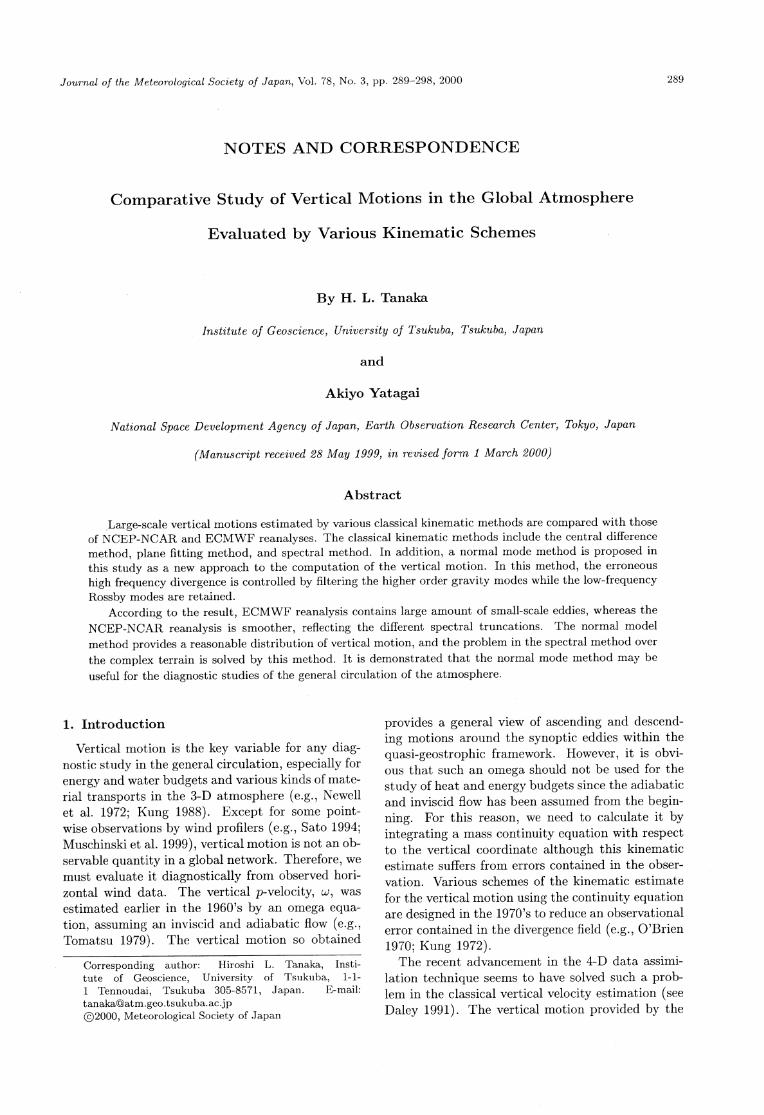
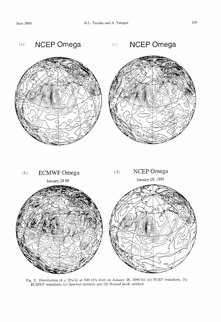
Figure 1 illustrates sea level pressure and 500 hPa height over the Pacific on 00002, January 28, 1989 by the NCEP-NCAR reanalysis. This specific day is chosen for the demonstration because two consecu-tive explosive cyclogenesis occurred at the Far East to yield a marked vertical motion as documented comprehensively by Hayasaki and Tanaka (1999). The low pressure system over the Sea of Okhotsk has a barotropic structure since the locations of the surface cyclone and 500hPa trough coincide with each other. Another low-pressure system is seen over Alaska extending southward to the north Pacific. Figure 2 compares w at the 500hPa level on

0000Z, January 28, 1989 for (a) NCEP-NCAR reanalysis, (b) ECMWF reanalysis, (c) spectral method, and (d) normal mode method. The grid-

ded horizontal winds of NCEP-NCAR reanalysis are used for all the computations in this study, except for w provided by ECMWF reanalysis. The ex-plosive cyclogenesis over Okhotsk yields a chain of pronounced upward (dashed lines) and downward (solid lines) motions over the northwestern Pacific. There is a downward motion associated with the cold advection behind the bomb over the Sea of Japan. Strong upward motion associated with the warm advection is seen along the eastern flank of the bomb induced by the southerly wind. Interest-ingly, another strong downward motion is detected near 170E downstream of the strong upward mo-tion. A detailed analysis has been documented for this descending motion that causes a pronounced and persistent blocking over Alaska (see Tanaka and Milkovich 1990; Tan and Curry 1993). The comparison of the vertical motions indicates

that the ECMWF reanalysis in Fig. 2(b) contains a bunch of small-scale structures of w compared with apparently smoother w by NCEP-NCAR in Fig. 2(a). The former has a model resolution of T-106, while the latter has T-62. The w by the spectral method truncated at T-42 in Fig. 2(c) is similar to the NCEP-NCAR reanalysis. Yet, the values are ex-tremely large over Tibet and Greenland as seen in Fig. 2(c). Although not shown, the Antarctic also indicates abnormally large vertical motions for the spectral method since the divergence is integrated from the bottom to top. The result by the normal mode method in Fig. 2(d) is smoother than the spec-tral method. The truncation seems to have filtered most of the small-scale structures since zonal wave

Fig. 1. Distribution of (a) sea level pressure (Pa) and (b) 500hPa height on January 28, 1989 for NCEP reanalyses.

NCEP SLP (b) 500hPa


Fig. 2. Distribution of w (Pa/s) at 500hPa level on January 28, 1989 for (a) NCEP reanalysis, (b) ECMWF reanalysis, (c) Spectral method, and (d) Normal mode method.

(a) NCEP Omega

(>>) ECMWF Omega

January 28 89

(() NCEF Omega

(<1) NCEP Omega

January 28, 1989


is truncated at m=15. It is important to note that there is no extreme values over Tibet, Greenland, and the Antarctic for the normal mode method.

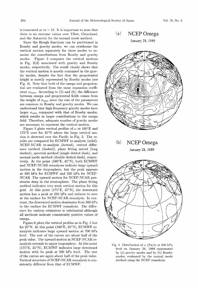
Since the Hough functions can be partitioned in Rossby and gravity modes, we can synthesize the vertical motion separately for those modes to ex-amine the contributions from Rossby and gravity modes. Figure 3 compares the vertical motions in Fig. 2(d) associated with gravity and Rossby modes, respectively. The result clearly shows that the vertical motion is mostly contained in the grav-ity modes, despite the fact that the geopotential height is mostly represented by Rossby modes (see Fig. 4). Note that both of the omega and geopoten-tial are evaluated from the same expansion coeffi-cient wnlm. According to (5) and (6), the difference between omega and geopotential fields comes from the weight of anim since the rest of the parameters are common to Rossby and gravity modes. We can understand that high-frequency gravity modes have larger anim compared with that of Rossby modes, which results in larger contributions to the omega field. Therefore, adequate number of gravity modes are necessary to represent the vertical motion. Figure 5 plots vertical profiles of w at 160E and

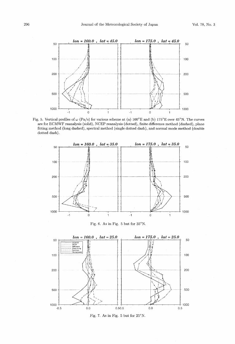
175E over for 45N where the large vertical mo-tion is detected over the Pacific in Fig. 2. The re-sults are compared for ECMWF re-analysis (solid), NCEP-NCAR re-analysis (dotted), central differ-ence method (dashed), plane fitting meted (long dashed), spectral method (single dotted dash), and normal mode method (double dotted dash), respec-tively. At the point (160E, 45N), both ECMWF and NCEP-NCAR reanalyses indicate large upward motion in the troposphere, but the peak appears at 500hPa for ECMWF and 350hPa for NCEP-NCAR. The upward motion for NCEP-NCAR pen-etrates deep in the stratosphere. The plane fitting method indicates very weak vertical motion for this grid. At this point (175E, 45N), the downward motion has a peak at 250hPa and reduces to zero at the surface for NCEP-NCAR reanalysis. In con-trast, the downward motion dominates from 300hPa to the surface for ECMWF reanalyses. The differ-ence for various estimators is substantial although all methods indicate consistently positive values of omega. Figure 6 plots the vertical profiles as in Fig. 5 but

for 35N. At this point (160E, 35N), ECMWF re-analysis indicates large upward motion at 700hPa level. The rest of the curves are about half of the peak value. The upward motion in NCEP-NCAR re-analysis extends to upper troposphere. At this point (175E, 35N), ECMWF indicates large downward motion with its peak at 500hPa level. The rest of the curves are again about half of the peak value. Vertical structure of NCEP-NCAR reanalyses is con-sistently different from that of ECMWF.

Fig. 3. Distribution of w (Pa/s) at 500hPa level on January 28, 1989 represented

by (a) gravity modes and by (b) Rossby modes, evaluated by the normal mode method using the NCEP reanalysis.

(a) NCEP Omega

January 28, 1989

(b) NCEP Omega

January 28, 1989


Figure 7 plots the vertical profiles as in Fig. 5, but for 25N. At this point (160E, 25N), ECMWF re-analysis indicates large upward motion at 700hPa level, whereas finite difference and plane fitting methods indicate downward motions. At this point (175E, 25N), ECMWF reanalysis and spectral method indicate large upward motion near the tropopause, whereas the upward motion is absent for NCEP-NCAR reanalysis. We note that the spec-tral method uses NCEP-NCAR reanalysis data, but apparently closer to the ECMWF reanalysis for this location. The difference for various estimators is substantial, but is within the range of the difference between ECMWF and NCEP-NCAR reanalyses.

4. Concluding summary

We first realize that the vertical motions provided by NCEP-NCAR and ECMWF reanalyses are sub-stantially different. The w in ECMWF contains large amounts of small-scale eddies, whereas NCEP-NCAR w is smoother than that of ECMWF, reflect-ing the different spectral truncations. It is noted (personal communication from Kistler of NCEP) that the NCEP-NCAR reanalysis is truncated by T-30 for the isobaric data although the assimilation model has the resolution of T-62. The central difference scheme and plane fitting

method provide a bunch of small-scale w as in ECMWF reanalysis, but those are considered as noise. In contrast, the spectral method and nor-mal mode method yield smooth w field as in NCEP-NCAR reanalysis. The smoothness in the spectral method may be caused by smooth divergence field in NCEP-NCAR reanalysis. On the other hand, the smooth result in the normal mode method is caused mostly by the severe truncations in the grav-ity modes. The difference in the magnitude for var-ious estimators is substantial. However, the dif-ference is within the range between ECMWF and NCEP-NCAR reanalyses. It is noted that the ver-tical structure of NCEP-NCAR reanalysis is clearly different from the rest of the results; the vertical motion tends to penetrate deep into the upper tro-posphere for NCEP-NCAR reanalysis.

In this study, a normal mode method is proposed as a new approach for the computation of the verti-cal motion. In this method, the divergence is com-puted analytically and is integrated from the top to bottom of the atmosphere also analytically as de-sired. It is demonstrated that the problem in the spectral method over the complex terrain is solved in this method. Only the assumption imposed by this method is a truncation, where we can selectively filter the higher frequency gravity modes while the low-frequency Rossby modes are retained. Since the upper air observations are carried out at 12-hour in-tervals, it is quite reasonable to truncate the higher-frequency gravity modes (noise) beyond the sam-

Fig. 4. As in Fig. 3 but for geopotential height represented by (a) gravity modes and by (b) Rossby modes.

(a) Geopotential Height

January 28, 1989

(b) Geopotential Height

January 28, 1989


Fig. 5. Verticall profiles of w (Pa/s) for various scheme at (a) 160E and (b) 175E over 45N. The curves are for ECMWF reanalysis (solid), NCEP reanalyses (dotted), finite difference method (dashed), plane fitting method (long dashed), spectral method (single dotted dash), and normal mode method (double dotted dash).

ion=160.0 lat=45.0 ion=175.0, kit=45.0

Fig. 6. As in Fig. 5 but for 35N.

ion=160.0, kit=35.0, ion=175.0, lat=35.0

Fig. 7. As in Fig. 5 but for 25N.

ion=160.0, iat=25.0 ion=175.0, lat=25.0


pling interval in the frequency domain. It may be important to note that the heat bud-

get analysis conducted with the w provided by the initialyzed global data, would produce the diabatic

process which is consistent with the model physics. Such a result of heat sources and sinks is, of course, not necessarily equal to that in the real atmosphere. A better estimate of the diabatic process should be based on a better estimate of the vertical motion evaluated from observations. We demonstrated that the normal mode method has less assumptions, and the anticipated error in divergence is controllable by a suitable truncation of the high-frequency gravity modes. In this regard, the method may be useful for the diagnostic studies of the general circulation of the atmosphere.

Acknowledgments

This research was supported by the Grant-in-Aid for Scientific Research from the Japanese Min-istry of Education, Science, Sports and Culture. The authors appreciates Ms. K. Honda and Mr. H. Kurasono for their technical assistance.

References

Daley, R., 1991: Atmospheric data analysis. CambridgeUniversity Press, 457pp.

Hayasaki, M. and H. L. Tanaka, 1999: A study of drasticwarming in the troposphere: A case study for thewinter of 1989 in Alaska. Tenki, 46, 123-135 (inJapanese).

Kasahara, A., 1984: The linear response of a stratifiedglobal atmosphere to tropical thermal forcing. J. At-mos. Sci., 41, 2217-2237.

Kung, E. C., 1972: A scheme for kinematic estimateof large-scale vertical motion with an upper-air net-work. Quart. J. Roy. Meteor. Soc., 98, 402-411.

-, 1988: Spectral energetics of the general circula-tion and time spectra of transient waves during theFGGE year. J. Climate, 1, 5-19.

Luo, Huibang and M. Yanai, 1983: The large-scale cir-culation and heat sources over the Tibetan plateauand surrounding areas during the early summer of1979. Part 1: Precipitation and Kinematic analysis.Mon. Wea. Rev., 111, 922-944.

Muschinski, A., P. B. Chilson, S. Kern, J. Nielinger,G. Schmidt and T. Prenosil, 1999: First frequency-domain interferometry observations of large-scalevertical motion in the atmosphere. J. Atmos. Sci.,56, 1248-1258.

Newell, R. E., J. W. Kidson, D. G. Vincent and G. J. Boer,1972: The general circulation of the tropical atmo-sphere and interaction with extratropical latitudes.The MIT Press, Vol. 1, 258pp., Vol. 2, 37lpp.

O'Brien, J. J., 1970: Alternative solutions to the classicalvertical velocity problem. J. Appl. Meteor., 9, 197-203.

Sasaki, Y. K. and L. P. Chang, 1985: Numerical solutionof the vertical structure equation in the normal modemethod. Mon. Wea. Rev., 113, 782-793.

Sato, K., 1994: A statistical study of the structure, sat-uration, and sources of inertia-gravity waves in thelower stratosphere observed with the MU radar. J.Atmos. Terr. Phys., 56, 755-774.

Tan, Y.-C. and J. A. Curry, 1993: A diagnostic studyof the evolution of an intense north American anti-cyclone during winter 1989. Mon. Wea. Rev., 121,961-975.

Tanaka, H. L. and E. C. Kung, 1988: Normal mode en-ergetics of the general circulation during the FGGE

year. J. Atmos. Sci., 45, 3723-3736.and M.F. Milkovich, 1990: A heat budget anal-

ysis of the polar troposphere in and around Alaskaduring the abnormal winter of 1988/89. Mon. Wea.Rev., 118, 1628-1639.

Tomatsu, K., 1979: Spectral energetics o f the Tropo-sphere and lower stratosphere. Advances in geo-physics, 21, 289-405.


運動学的に推定した大規模鉛直流の比較研究

田中博

(筑波大学地球科学系)

谷田貝亜紀代

(宇宙開発事業団地球観測データ解析研究センター)

本研究では、大規模鉛直流を運動学的に推定するいくつかの計算法を相互に比較し、それらの結果を

NCEP-NCARおよびECMWF再解析による鉛直流の値と比較した。比較した計算法は中央差分法、平面

近似法、スペクトル法の3通りであるが、スペクトル法を3次元に拡張したノーマルモード法による鉛直

流計算法を新たに考案し、他の結果と比較した。ノーマルモード法では、計算はすべて解析的であり、発

散誤差の大きい重力波の固有周波数を基準にして波数切断を決めることができる。

鉛直流の相互比較の結果、ECMWF再解析には小さいスケールの強い鉛直流が目立つのに対し、NCEP-

NCAR再解析ではそれが平滑化されており、鉛直構造も異なるという特徴が見られた。ノーマルモード法

は、複雑地形上でも極端な鉛直流の値を示さないので、大気大循環の解析的研究に有用であることが確か

められた。

Documents

Journal of the Meteorological Society of Japan, Vol. 78