Asymptotic behaviour methods for the HeatEquation. Convergence to the Gaussian

Juan Luis VázquezUniversidad Autónoma de Madrid

2017

Abstract

In this expository work we discuss the asymptotic behaviour of the solutions of the classicalheat equation posed in the whole Euclidean space. After an introductory review of the mainfacts on the existence and properties of solutions, we proceed with the proofs of convergenceto the Gaussian fundamental solution, a result that holds for all integrable solutions, andrepresents in the PDE setting the Central Limit Theorem of probability. We present severalmethods of proof: first, the scaling method. Then several versions of the representationmethod. This is followed by the functional analysis approach that leads to the famous relatedequations, Fokker-Planck and Ornstein-Uhlenbeck. The analysis of this connection is alsogiven in rather complete form here. Finally, we present the Boltzmann entropy method,coming from kinetic equations.The different methods are interesting because of the possible extension to prove the asymptoticbehaviour or stabilization analysis for more general equations, linear or nonlinear. It alldepends a lot on the particular features, and only one or some of the methods work in eachcase. Other settings of the Heat Equation are briefly discussed in Section 9 and a longermention of results for different equations is done in Section 10.

2010 Mathematics Subject Classification: 35K05, 35K08.

Keywords and phrases: Heat equation, asymptotic behaviour, convergence to the Gaussian solu-tion.

1

arX

iv:1

706.

1003

4v2

[m

ath.

AP]

20

Sep

2017

Contents

1 The Cauchy Problem in RN for the Heat Equation 3

2 Asymptotic convergence to the Gaussian 8

3 Proof of convergence by scaling 10

4 Asymptotic convergence to the Gaussian via representation 11

5 Improved convergence for distributions with second moment 16

6 Functional Analysis approach for Heat Equations 19

7 Calculation of spectrum. Refined asymptotics 23

8 Convergence via the Boltzmann entropy approach 25

9 Brief review of other heat equation problems 26

10 Application to other diffusion equations 30

11 Historical comments 32

2

1 The Cauchy Problem in RN for the Heat Equation

The classical heat equation (HE) ∂tu = ∆u, is one of the most important objects in the theory ofpartial differential equations, and it has great relevance in the applied sciences. It has been devel-oped since the seminal work of J. Fourier, 1822, [32], to describe phenomena of heat transport anddiffusion in many contexts. The great progress of the mathematical theory in these two centurieshas had a strong influence not only on PDEs, but also on Probability, Functional Analysis, aswell as Numerics. It now has well-established connections with other subjects like viscous fluids,differential geometry, image processing or finance. See more on motivation in standard textbooks,like [31, 58] or in the survey paper [69].

The heat equation enjoys a well developed theory that has many distinctive features. It can besolved in many settings, suitable for different interests, that lead to quite different results and usedifferent tools. In this paper we will study the most typical setting, the Cauchy Problem posedin RN , N ≥ 1:

(CPHE)

∂tu = ∆u in RN × (0,∞)

u(x, 0) = u0(x) in RN ,

with initial data u0 ∈ L1(RN ). The equation appears in the theory of Probability and StochasticProcesses as the PDE description of Brownian motion, and in that application the function u(·, t)denotes the probability density of the process at time t, hence it must be nonnegative and the totalintegral

∫u(x, t) dx, often called the mass, must be one. Such restrictions on sign and integral

are not needed in the analytical study, and the extra generality is convenient both for the theoryand for a number of other applications.

The first question to be addressed by mathematicians is to find appropriate functional spacesto solve this problem and to prove that it is a well-posed problem in the sense of Hadamard’sdefinition (existence, uniqueness and stability). In tackling such a problem we will be luckyenough to find a very explicit representation of the solution by means of the so-called “fundamentalsolution” procedure.

Definition. We call fundamental solution of the HE in RN the solution of the equation withinitial data a “Dirac delta”:

(FS)

∂tU = ∆U en RN × (0,∞)

U(x, 0) = δ0(x) en RN .

In probabilistic terms, we start from a unit point mass distribution concentrated at the originx0 = 0, and we look for the way is expands with time according to the heat equation.

Exercise 1. (i) Prove by the method of Fourier Transform that the fundamental solution is givenby the formula

(GF) U(x, t) = (4πt)−N2 e−

|x|24t .

Sketch. The Fourier transform of U satisfies ∂tU = −ξ2U with U(ξ, 0) = 1, hence U(ξ, t) = e−ξ2t.

Then, invert the Fourier transform.

(ii) Prove that U(x, t)→ δ0(x) when t→ 0 in the sense of distributions, that is∫RN

U(x, t)φ(x)dx → < δ0, φ >:= φ(0), for all φ ∈ C∞c (RN ), as t→∞.

3

(iii) Prove that for every sequence tn → 0 the functional sequence U(x, tn) is a C∞ approximationof the identity.

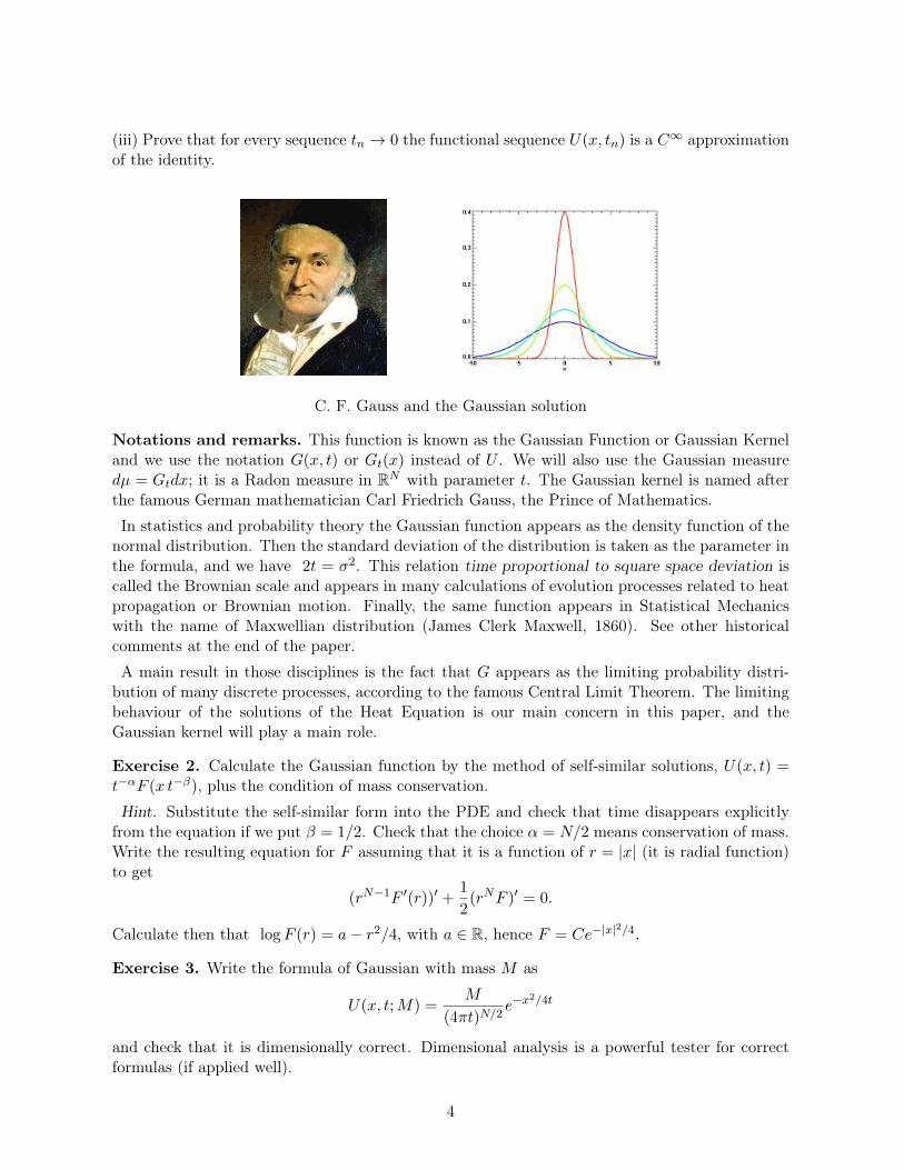
C. F. Gauss and the Gaussian solution

Notations and remarks. This function is known as the Gaussian Function or Gaussian Kerneland we use the notation G(x, t) or Gt(x) instead of U . We will also use the Gaussian measuredµ = Gtdx; it is a Radon measure in RN with parameter t. The Gaussian kernel is named afterthe famous German mathematician Carl Friedrich Gauss, the Prince of Mathematics.

In statistics and probability theory the Gaussian function appears as the density function of thenormal distribution. Then the standard deviation of the distribution is taken as the parameter inthe formula, and we have 2t = σ2. This relation time proportional to square space deviation iscalled the Brownian scale and appears in many calculations of evolution processes related to heatpropagation or Brownian motion. Finally, the same function appears in Statistical Mechanicswith the name of Maxwellian distribution (James Clerk Maxwell, 1860). See other historicalcomments at the end of the paper.

A main result in those disciplines is the fact that G appears as the limiting probability distri-bution of many discrete processes, according to the famous Central Limit Theorem. The limitingbehaviour of the solutions of the Heat Equation is our main concern in this paper, and theGaussian kernel will play a main role.

Exercise 2. Calculate the Gaussian function by the method of self-similar solutions, U(x, t) =t−αF (x t−β), plus the condition of mass conservation.

Hint. Substitute the self-similar form into the PDE and check that time disappears explicitlyfrom the equation if we put β = 1/2. Check that the choice α = N/2 means conservation of mass.Write the resulting equation for F assuming that it is a function of r = |x| (it is radial function)to get

(rN−1F ′(r))′ +1

2(rNF )′ = 0.

Calculate then that logF (r) = a− r2/4, with a ∈ R, hence F = Ce−|x|2/4.

Exercise 3. Write the formula of Gaussian with mass M as

U(x, t;M) =M

(4πt)N/2e−x

2/4t

and check that it is dimensionally correct. Dimensional analysis is a powerful tester for correctformulas (if applied well).

4

Exercise 4. Gaussian Representation Formula. Show that if u0 ∈ C(RN ) and is bounded,then

(GRF) u(x, t) = (U ∗ u0)(x, t) := (4πt)−N2

∫RN

u0(y)e−|x−y|2

4t dy

is a solution of the heat equation wit initial data u0. Check that it is C∞ function of x and t forevery x ∈ RN and t > 0. Prove that u(x, t)→ u0(x) pointwise when t→ 0.

(ii) Prove that the initial data is taken uniformly if u0 ∈ BUC(RN ), the space of bounded anduniformly continuous functions in RN .(iii*) Consider whether the boundedness condition of point (i) can be relaxed or eliminated.

Exercise 5. Prove that formula (GRF) is still valid when the initial data belong to Lp(RN ),1 ≤ p ≤ ∞.

(ii) What is the regularity of the solution?

(iii) In which sense are the initial data taken?

Exercise 6. (i) Prove that (GRF) generates a continuous contraction semigroup in the followingBanach spaces

X = BUC(RN ), L2(RN ), Lp(RN ), 1 < p <∞ ,

by means of the definition St : X → X, Stu0 = u(·, t), where u is the solution of the heat equationwith initial data u0.

Sketch. What you have to check is that as function of time t, f(t) := Stu0 belongs to C([0,∞ :X), that St ∗ Ss = St+s, and also Stu0 → u0 as t → 0 in X. Moreover, contraction means that‖Stu0‖X ≤ ‖u0‖X for every t > 0 and every u0 ∈ X.

(ii) Study in which sense the semigroups agree (explain if they are the same or not). You maydefine the core of the semigroup by restricting it to a nice and dense set of functions, and thenexplain how the concept of density is used to recover the complete semigroup in the above spaces.

Notation. We will often write u(t) instead of u(·, t) for brevity in the hope that no confusionwill arise. Hence, u(t) is a function of x for every fixed t.

Exercise 7. (i) Prove that for p = 1 we have the stronger property of mass conservation

(MC)∫RN

u(x, t) dx =

∫RN

u0(x) dx ,

for all data in L1(RN ).

(ii) Note that this law also holds for signed solutions. Show that the version with absolute valueis not valid for signed solutions by means of an example (superposition of two Gaussians)

(iii) Prove on the fundamental solution that the Lp-integrals with p > 1 are not conserved andcheck the rate of decay they exhibit. Terminology: The p energy is

∫|u|p dx. Those p-energies

are not conserved because they “undergo dissipation”.

(iv*) The curious reader may want to learn more about that dissipation and how to measure itaccurately. Any ideas?

5

Exercise 8. Conservation of moments. (i) We define the first (signed) moment as the vectorquantity

(1.1) N1(u(t)) =

∫RN

xu(x, t) dx ,

which in principle evolves with time. Prove that this quantity is actually conserved in time forany solution of the HE with initial data such that

∫(1 + |x|)|u0(x)| dx is finite.

(ii) For data such that∫|x|2 |u0(x)| dx is finite, we define the second moment as the scalar

time-dependent quantity

(1.2) N2(u(t)) =

∫RN|x|2 u(x, t) dx .

Prove that this quantity is not conserved in time for solutions of the HE, and in fact

(1.3) N2(u(t)) = N2(u0) + 2Nt .

(Recall here that N is the space dimension). These results will be important to understand thefiner versions of the asymptotic convergence to the Gaussian. Deeper analysis proves that theonly integral quantities conserved by the solutions of the Heat Equation are the mass and thefirst moment.

Exercise 9. (i) Prove the so-called ultra-contractive estimates, also called smoothing effects.They allow to pass from data in Lp to solutions u(t) in L∞ for every t > 0. More precisely, provethat there exists a constant C = C(p,N) such that for every u0 ∈ Lp(RN )

‖u(t)‖∞ ≤ C‖u0‖ptN/2p

.

We may say that the constant is universal since it does not depend of the particular solution wetake.

(ii) Calculate the exponent N/2p using only dimensional calculus.

Exercise 10. Regularity. (i) Prove that there exists a universal constant C = C(p,N) > 0such that for every p ≥ 1 and every t > 0

‖du(t)

dt‖p ≤ C

‖u0‖pt

.

(ii) Prove that for nonnegative solutions we have a stronger pointwise inequality

∂u

∂t≥ −C1

u

twith C1 = N/2 .

Prove that this constant is optimal. Hint. Check the properties first for the fundamental solution,then use convolution.

(iii) Prove that for every t > 0 the x-derivatives of u satisfy∣∣∣∣ ∂∂xiu(x, t)

∣∣∣∣ ≤ C ||u0||L∞t12

.

6

Obtain a similar estimate for data in Lp(RN).

(iv) Check that the dimensions are all correct in these formulas.

Exercise 11. Gaussian Representation Formula with measure data. (i) Prove that therepresentation formula can be used with any bounded Radon measure as initial data, in the form

(GRFm) u(x, t) = (Gt ∗ µ)(x, t) := (4πt)−N2

∫RN

e−|x−y|2

4t dµ(y) .

(ii) Prove that it produces a classical solution of the HE for all t > 0 and that the a prioriestimates hold with the L1 norm of u0 replaced by the total mass of the measure, |µ(RN )| =

∫|dµ|.

(iii) Prove that the initial data are taken in the weak sense of measures.

(iv) Observe that the fundamental solution U = Gt falls into this class.

Exercise 12. (i) Find explicit solutions of polynomial type of heat equation. Suggestion: try thesolution types

u = A0(x), u = A0(x) +A1(x)t, u = A0(x) +A1(x)t+A2(x)t2, . . .

Find all the solutions of the first two types. Maybe the best known solutions in this class areu = 1 and u = |x|2 + 2Nt.

(ii) Prove that they also satisfy the representation formula, even though they are not integrableor bounded.

The general theory says that the (GRF) holds for all initial data which are locally boundedmeasures µ with a weighted integrability condition∫

RNec|x|

2 |dµ(x)| <∞ for some c > 0 ,

see [70], but we will not use that sharp result in these notes. We will only point out the followingexample of blow-up solution with very large growth as |x| → ∞

(1.4) Ub(x, t) = C (T − t)−N/2e|x|2/4(T−t).

Exercise 13. Check that Ub is a classical solution of the heat equation for −∞ < t < T andblows up everywhere in x as t→ T .

Exercise 14. Construction of new solutions.

(i) Show that if u(x, t) is a solution of the heat equation, so are u1 = ∂tu, and u2 = ∂xiu.

(ii) Show that if u(x, t) is a solution of the heat equation in 1D then so is also u3 =∫ x−∞ u(s, t) ds.

(iii) Prove that if u(x, t) is a solution of the heat equation so is also

v(x, t) = Au(Bx,B2t)

for any choice of the parameters A and B. This is called the scaling property. A and B need notbe positive.

(v*) Show that if u(x, t) is a solution of the heat equation, then so is also

v(x, t) = xux + 2tut .

This is a 1D notation. But the result is valid in any dimension if the notation is correctlyinterpreted.

7

2 Asymptotic convergence to the Gaussian

The main result on the asymptotic behaviour of general integrable solutions of the heat equationconsists in proving that they look increasingly like the fundamental solution. Since this solutiongoes to zero uniformly with time, the estimate of the convergence has to take into account thatfact and compensate for it. This happens by considering a renormalized error that divides thestandard error in some norm by the size of the Gaussian solution U(t) = Gt in the same norm.For instance, in the case of the sup norm we know that

‖Gt‖L∞(RN ) = Ct−N/2, ‖Gt‖L1(RN ) = 1.

This is the basic result we want to prove

Theorem 2.1 Let u0 ∈ L1(RN ) and let∫u0(x)dx = M be its mass. Then the solution u(t) =

u(·, t) of the HE in the whole space ends up by looking like M times the fundamental solutionU(t) = Gt in the sense that

(2.1) limt→∞‖u(t)−MGt‖1 → 0

and also that

(2.2) limt→∞

tN/2‖u(t)−MGt‖∞ → 0 .

By interpolation we get the convergence result for all Lp norms

(2.3) limt→∞

tN(p−1)/2p‖u(t)−MGt‖Lp(RN ) → 0 .

for all 1 ≤ p ≤ ∞.

We add important information to this result in a series of remarks.

• First, one comment about the spatial domain. The fact that we are working in the whole spaceis crucial for the result of Theorem 2.1. The behaviour of the solutions of the heat equationposed in a bounded domain with different kinds of boundary conditions is also known, and theasymptotic behaviour does not follow the Gaussian pattern.

• As we will see below, convergence to the Gaussian happens on the condition that the databelong to the class of integrable functions, that can be extended without problem to boundedRadon measures. This is actually no news since the theory says that the solution correspondingto an initial measure µ ∈ M(RN ) is integrable and bounded for any positive time, so we maychange the origin of time and make the assumption of integrable and bounded data. But we pointout the some of the proofs work directly for measures without any problem.

• We recall that it is usually assumed that u ≥ 0 on physical grounds but such assumption is notat all needed for the analytical study of this paper. Thus, the basic result holds also for signedsolutions even if the total integral is negative, M ≤ 0. There is no change in the proofs. We mayalso put M = 1 by linearity as long as M 6= 0.

• M = 0 is a special case that deserves attention: even if Theorem (2.1) is true, the statementdoes not imply that the solution looks asymptotically like a Gaussian; to be more precise, it onlysays that the previous first-order approximation disappears. If we want more precise details about

8

what the solution looks like, we have to search further to identify the terms that may give us thesize and shape of such a solution. This question will be addressed below. For the moment let uspoint out that differentiation in xi of the Heat Kernel produces a new solution with zero integral

ui(x, t) = ∂xiGt(x) = C t−(N+2)/2xi e−|x|2/4t ,

to which we can apply the above comments. In particular,

tN/2ui(x, t) = O(t−1/2) ,

where O(·) is the Landau O-notation for orders of magnitude.

• It must be stressed that convergence to the Gaussian does not hold for other data. Maybethe simplest example of solution that does not approach the Gaussian is given by any non zeroconstant solution, but it could be objected that L∞(RN ) is very far from L1(RN ). Actually, thesame happens for all Lp(RN ) spaces, p > 1. Indeed, a simple argument based on approximationand comparison shows that for any u0 ≥ 0 with

∫u0(x) dx = +∞ we have

limt→∞

tN/2u(x, t) = +∞

everywhere in x ∈ RN (and the divergence is locally uniform).

• The way different classes of non-integrable solutions actually behave for large time is an inter-esting question that we will not address here. Thus, the reader may prove using the convolutionformula that for locally integrable data that converge to a constant C as |x| → ∞ the solutionu(x, t) stabilizes to that constant as t → ∞. Taking growing data may produce solutions thattend to infinity with time, like the 1D family of travelling waves

UTW (x, t) = C ec2t+cx

defined for real constants C, c 6= 0. A more extreme case is the blow-up solution Ub(x, t) of formula(1.4) that not only does not stay bounded with time, it even blows up in finite time.

• About the three convergence results of the Theorem, it is clear that (2.3) follows from (2.1)and (2.2). Now, what is interesting is that (2.2) follows from (2.1) and the smoothing effect(Exercise 9). We ask the reader to prove this fact. Hint: use (2.1) between 0 and t/2 and thenthe smoothing effect between t/2 and t.

• It is interesting to note that the convergence in L1 norm of formula (2.1) can be formulatedwithout mention to the existence of a fundamental solution in the following form:

Alternative Theorem. Let u(t) and v(t) be any two solutions of the Cauchy problem for theHE in the whole space, and let us assume that their initial data satisfy

∫u0 dx =

∫v0 dx. Then

we have

(2.4) limt→∞‖u(t)− v(t)‖1 → 0 .

We could use a similar approach for the L∞ estimate but some Gaussian information appearsin the weight tN/2. The alternative approach has been first remarked by specialists in stochasticprocesses of Brownian type, and it is known as a mixing property. It has been generalized tomany variants of the heat equation.

9

3 Proof of convergence by scaling

There are many approaches to the proof of the main result, and we will show some of the bestknown below. They are interesting for their possible extension to similar asymptotic results forother equations, both linear and nonlinear, see Sections 9 and 10. The first proof we give is basedon scaling arguments. In the proposed method the proof is divided into 5 steps.

Step 1. Scaling transformation. It is easy to check that the HE is invariant under the followingone-parameter family of transformations Tk defined on space-time functions by the formula

Tku(x, t) = kNu(kx, k2t), k > 0,

see also Exercise 14 (iii). This transformation maps solutions u into new solutions uk = Tku,called rescalings of the original solution. It also conserves the mass of the solutions∫

RNTku(x, t) dx =

∫RN

u(y, k2t) dy = constant.

Step 2. Uniform estimates. The estimates proved on the general solutions in Section 1 implythat the whole family uk is uniformly bounded in space and time if time is not so small: x ∈ RNand t ≥ t1 > 0 (cf. Exercise 9). They also have uniform estimates on all derivatives under thesame restriction on time (cf. Exercise 10).

Step 3. Limit problem. We can now use functional compactness and pass to the limit k →∞ along suitable subsequences to obtain a function U(x, t) that satisfies the same estimatesmentioned above and is a weak solution of the HE in Q = RN × (0,∞). By the estimates onderivatives the solution is classical. The convergence takes place locally in Q in the sup norm forthe functions and their space and time derivatives.

Step 4. Identifying the limit. We now have to check that the limit solution U(x, t) has the samemass M as the sequence uk and that is takes the Dirac delta as initial data. By uniqueness forsolutions with measure data (which we accept as part of the theory) we will then conclude thatU(x, t) is just a fundamental solution, U(x, t) = M Gt.

(i) The proof of this step is best done when u0 is nonnegative, compactly supported and bounded,since in that case the solution is bounded above by constant times the fundamental solution,|u(x, t)| ≤ C G(x, t+ 1). Applying the transformation we get

|uk(x, t)| ≤ C Tk(G(x, t+ 1)) = C G(x, t+ k−2).

This means a uniform control from above of the mass of all the tail mass of all the solutions uk,by which we mean the mass lying in exterior regions of space. Such control allows to avoid theloss of mass that could occur in the limit by Fatou’s Theorem. Hence, the mass of U is the same,i.e., M .

The convergence of U to M δ(x) as t→ 0 happens because uk(x, 0)→M δ(x), and the previoustail analysis shows that U takes zero initial values for x 6= 0.

(ii) To recover the same result for a general u0 ≥ we use approximation by data as above andthen the L1 contraction of the heat semigroup. For signed solutions, separate the positive andnegative parts of the data and solve separately.

10

Step 5. Recovering the result. (i) We now use the convergence of the rescaled solutions at afixed time, say t = 1,

limk→∞

|uk(x, 1)−MG1(x)| → 0.

This convergence takes place locally in RN in all Lp norms. By the tail analysis, it also happensin L1(RN ). But since the derivatives are also uniformly bounded we have also an L∞ estimate.

(ii) We now use the meaning to the transformation Tk and write k = t1/21 to get

limt1→∞

|tN/21 u(xt1/21 , t1)−MG1(x)| → 0.

But this is just the result we wanted to prove after writing x = y t−1/21 and observing that

Gt1(y) = t−N/21 G1(x). Similarly for the L1 norm.

This 5-step proof is taken from paper [48], where it was applied to the p-Laplacian equation. Seewhole details for the porous medium equation in the book [66]. It has had further applicability.

Exercise 15. Fill in the details of the above proof.

4 Asymptotic convergence to the Gaussian via representation

The second proof we give of the main result, Theorem 2.1, is based on the examination of the errorin terms of the representation formula. This is a very direct approach, but it needs a previous step,whereby the proof is done under the further restriction that the data have a finite first moment.Then the convergence result is more precise and quantitative. This particular case has an interestin itself since it shows the importance of controlling the first moment of a mass distribution. Wealready know that the first moment is associated to a conserved quantity (see Exercise 8).

Theorem 4.1 Under the assumptions that u0 ∈ L1(RN ) and that the first absolute moment isfinite

(4.1) N1 =

∫|u0(y)y| dy <∞ ,

we get the convergence

(4.2) tN/2|u(x, t)−MGt(x)| ≤ CN1t−1/2 ,

as well as

(4.3) ‖u(x, t)−MGt(x)‖L1(RN ) ≤ CN1t−1/2 .

The rate O(t−1/2) is optimal under such assumptions.

Proof. (i) We may perform the proof under the further restriction that u0 ≥ 0. For a signedsolution we must only separate the positive and negative parts of the data and apply the resultsto both partial solutions.

11

(ii) Let us do first the sup convergence. We have

u(x, t)−MGt(x) =

∫u0(y)Gt(x− y) dy −Gt(x)

∫u0(y) dy

=

∫u0(y)(Gt(x− y)−Gt(x)) dy

=

∫u0(y)

(∫ 1

0∂s(Gt(x− sy)) ds

)dy

= Ct−N/2∫dy

∫ 1

0ds u0(y)〈y, x− sy

2t〉e−|x−sy|2/4t

with C = (4π)−N/2. Consider the piece of the integrand of the form

f =x− syt1/2

e−|x−sy|2/4t = ξe−|ξ|

2/4 ,

where we have put ξ = (x − sy)/t1/2. We observe that the vector function f is bounded by anumerical constant, hence

|u(x, t)−MGt(x)| ≤ C1t−(N+1)/2

∫|u0(y)y| dy .

Taking into account that Gt is of order t−N/2 in sup norm, we write the result as (4.2), andC = C(N) is a universal constant.

(iii) For the L1 convergence we start in the same way and arrive at

u(x, t)−MGt(x) = C t−N/2∫dy

∫ 1

0ds u0(y)〈y, x− sy

2t〉e−(x−sy)2/4t .

Now we integrate to get

‖u(x, t)−MGt(x)‖1 ≤ C t−N/2∫RN

dx

∫RN

dy

∫ 1

0ds |u0(y)y| |x− sy|

2te−|x−sy|

2/4t

= C

∫RN

dy

∫ 1

0ds |u0(y)y|t−1/2(

∫RN

t−N/2|x− sy|t1/2

e−|x−sy|2/4t dx)

With the change of variables x− sy = t1/2ξ we already know that the last integral is a constantindependent of u, hence the formula for the L1 error. Note that now we are speaking of massesand we do not need any renormalization time factor.

(iv) We ask the reader to prove the optimality as an exercise.

Exercise 16. Take as solution the Gaussian after a space displacement, u(x, t) = G(x+h, t), andfind the convergence rate to be exactly O(t−1/2). This is just a calculus exercise but attention todetails is needed. Hint: Write

G(x+ h, t) = Gt(x) + h∂xGt(x) +h2

2D2xGt(ξ)

(where ξ = x+ sh, 0 < s < 1), and check that

∂xGt(x) = Ct−(N+1)/2 ξe−ξ2/4 = O(t−(N+1)/2) ,

12

uniformly in x, and D2xGt(ξ) = O(t−(N+2)/2) uniformly in x. This exercise shows that the term

h∂xGt(x) is the precise corrector with relative error O(t−1/2). We could continue the analysis byexpanding in Taylor series with further terms, see below. Exact correctors and longer expansionsfor general solutions will be done later in Section 7 by the methods of Functional Analysis.

Remark. The factor tN/2 is the appropriate weight to consider relative error. We point out thatthe more precise relative error formula

(4.4) εrel(t) =|u(x, t)−Gt(x)|

Gt(x)

does not admit a sup bound, as can be observed by choosing u(x, t) = Gt(x−h) for some constanth since then

εrel(t) = |exh/2te−h2/4t − 1| ,

which is not even bounded. It is then quite good that our weaker form does admit a goodestimate. Same happens for the L1 norm. This comment wants to show that error calculationswith Gaussians are delicate because of the tail (i.e., the behaviour for large |x|.

• Proof of Theorem 2.1 in this approach. Given an initial function u0 ∈ L1(RN ) without anyassumption on the first moment, we argue by approximation plus the triangular inequality. Inthe end we get a convergence result, but less precise. To quote, if u0 is integrable with integralM and let us fix an error δ > 0. First, we find an approximation u01 with compact support andsuch that

‖u0 − u01‖1 < δ.

Due to the already mentioned effect L1 → L∞, and applied to the solution u− u1, we know thatfor all t > 0

‖u(t)− u1(t)‖∞ < C δ t−N/2 .

On the other hand, we have just proved that for data with finite moment:

‖u1(t)−M1Gt‖∞ ≤ CN1δ t−(N+1)/2 .

In this way, for sufficiently large t (depending on δ) we have

tN/2‖u1(t)−M1Gt‖∞ ≤ Cδ

with C a universal constant. Next se recall that |M −M1| ≤ δ as well as Gt ≤ Ct−N/2. Usingthe triangular inequality we arrive at

(4.5) limt→∞

tN/2‖u(t)−MGt‖∞ = 0 ,

which ends the proof.

Remark. In the general conditions of Theorem 2.1 we still obtain convergence, but we no longerobtain a rate. In fact, we show next that no convergence speed can be found without furtherinformation on the data other than integrability of u0.

13

4.1 No explicit rates for general data. Counterexample

Let us explain how the lack of a rate for the whole class of L1 functions is proved. Given anydecreasing and positive rate function φ such that φ(t)→ 0 as t→∞ we construct a modificationof the Gaussian kernel that produces a solution with the same mass M = 1 that satisfies theformula

tN/2‖u(x, t)−Gt(x)‖∞ ≥ nφ(tn)

at a sequence of times tn → ∞ to be chosen. The idea is to find a choice of small massesm1,m2, . . . with

∑nmn = δ < 1, and locations xn with |xn| = rn →∞ and consider the solution

u(x, t) = (1− δ)Gt(x) +∞∑n=1

mnGt(x− xn) .

The error u(x, t)−Gt(x) is calculated at x = 0 as

(4πt)N/2|u(0, t)−Gt(0)| = |δ −∞∑n=1

mne−x2n/4t| =

∞∑n=1

mn(1− e−x2n/4t) .

Put mn = 2−n (any other summable series will do). Choose iteratively tn and xn as follows.Given choices for the steps 1, 2, . . . , n − 1 , pick tn to be much larger than tn−1 and such thatφ(tn) ≤ mn/2n. This is where we use that φ(t) tends to zero, even if it may decrease in a veryslow way. Choose now |xn| = rn so large that e−r

2n/4tn < 1/2. Essentially, the mass has to be

displaced at distance equal or larger than O(t1/2n ). Then

mn(1− e−x2n/4tn) ≥ nφ(tn) .

Let us make some further practical calculations (with no precise scope in mind): Let for exampleφ(t) = t−ε. Choose mn = 2−n. Then tεn ≥ 2n,

tn ∼ 2n/ε, rn ∼ 2n/2ε

and the mass in the outer region |x| ≥ rn is approximately 2−n; hence such a mass is M(r) ∼r−2ε , which is not so small if ε→ 0.

4.2 Infinite propagation in space

The representation formula immediately shows that a solution u corresponding to nonnegativeinitial data will be strictly positive at all points x ∈ RN for any time t > 0. The infinite speedof propagation of the heat equation with the instantaneous formation of a thin tail at infinityis considered an un-physical property by many authors, one of the not many drawbacks of thiswonderful equation. However, it is essential to the equation and creates some curious effects.

• Spatial tails for positive solutions. Let us examine the precise form of the tail in thesimplest case where u0 has compact support. For simplicity and w.l.o.g. we assume that u0 issupported in the ball BR of radius R > 0 centered at x = 0. Take x1 ∈ RN such that |x1| = r1 > 1,say x1 = r1e1. Then the representation formula implies that a bound from above is obtained bydisplacing all the mass to the nearest point to x1 inside BR, which is x′0 = Re1, and we get

u(x1, t) ≤M Gt(x1 − x0) =M

(4πt)N/2e−(|x1|−R)2/4t .

14

Moving all the mass to x′′0 = −Re1 we get the lower bound.

u(x1, t) ≥M Gt(x1 − x′0) =M

(4πt)N/2e−(|x1|+R)2/4t .

Both are clearly optimal in this context. Since the equation is invariant under rotations the resultholds for all x such that |x| > 1 instead of our restricted choice of x1. Moreover, we see that theratio of both estimates tends to infinity as |x| → ∞. It is therefore convenient to take logarithms,and then we easily get a general formula where BR is centered at xc with |xc| = Rc

Proposition 4.2 Let u0 be supported in the ball BR(xc) and let M =∫u0(x) dx. Then for every

t > 0 and every x 6= BR(xc) we have

(4.6)N

2log(4πt) +

1

4t(|x− xc|+R)2 ≤ − log(u(x, t)/M) ≤ N

2log(4πt) +

1

4t(|x− xc| −R)2 .

It follows that

(4.7) lim|x|→∞

log(u(x, t)/M)

|x|2= − 1

4t.

We conclude that in first approximation the tail at infinity of all solutions with compactlysupported initial data is universal in shape and depends only on the mass of the data and time.Of course, the second term in the expansion depends also on the radii Rc and R.

Another observation is that the asymptotic space behaviour allows to calculate the time elapsedsince the solution had compact support (if we already know the mass M).

Let us also remark that solutions with more general nonnegative data can have other type oftails and we invite the reader to calculate some of them, both for integrable and non-integrabledata. Here is an example that decays like a simple exponential.

Exercise 17. Consider the heat equation in 1D. Show that when u0 is integrable, positive andbounded and u0(x) = e−x for x ≥ 0, then for all times

limx→∞

exu(x, t) = et.

Sketch: Putting u0(x) = 0 for x < 0 for simplicity, use the representation formula to write

ex−tu(x, t) =1

(4πt)1/2

∫ x

−∞e−(y−2t)

2/4tdy

Let then x→∞. You may also use the explicit solution U(x, t) = et−x+c.

In any case the behaviour described in Proposition 4.2 is the minimal one for nonnegativesolutions.

• Signed solutions do not become everywhere positive.The square exponential tail behaviour of the fundamental solution has more curious consequences.Thus, if a signed solution u(x, t) has initial data such that the mass of the positive part M+ =∫u+0 (x)dx is larger than the mass of the negative part M− =

∫u−0 (x)dx then we know that it

converges as t→∞ to the positive Gaussian MGt with M = M+ −M− > 0 so that

(4.8) limt→∞

tN/2u(x, t) = (4π)−N/2M > 0.

15

for every x ∈ RN . It would be natural to expect that when M+ is much larger than M− then thesolution u is indeed positive everywhere for large enough finite times. Now, this is true in mostof the space because of the previous convergence, but it is not true in all the space.

Exercise 18. (i) Take N = 1. Show that for the choice u0(x) = δ(x)− ε δ(x− 1) (a combinationof delta functions) the solution u is positive on the right of a line x = r(t) and negative forx > r(t). Show that for large times r(t) ∼ 2 log(1/ε)t.

Remark. We see that the problem arises at the far away tail. Of course, u(x, t) becomes positivefor large times at all points located at or less than the typical distance, |x| ≤ Ct1/2.(ii) Show that a similar result is true for integrable data if u0 is positive for x < 0 and negative

for x > 1, and zero in the middle. Show in particular that u(x, t) < 0 if x > 2t log(1/ε) + 1/2.

(iii) State similar results in several dimensions.

5 Improved convergence for distributions with second moment

Better convergence rates can be obtained by asking a better decay at infinity of u0. The tech-nical condition we use is having a finite second moment, a condition that is very popular in theliterature. In probability this is known as having a finite variation. The motivating example isdescribed next.

Exercise 19. Consider a time displacement of the fundamental solution and show that u(x, t) =G(x, t+ t0) has the precise convergence rate O(1/t) towards G(x, t).

The result we prove is as follows.

Theorem 5.1 Under the assumptions that u0 ∈ L1(RN ) and that the signed first moment

(5.1) N1,i =

∫RN

yi u0(y) dy

is finite (for all coordinates), as well as the second moment:

(5.2) N2 =

∫RN

y2 |u0|(y) dy <∞,

we get the convergence

(5.3) tN/2|u(x, t)−M Gt(x) +∑i

N1,i ∂xiGt(x)| ≤ CN2 t−1 ,

and

(5.4) ‖u(x, t)−M Gt(x) +∑i

N1,i ∂xiGt(x)‖L1(RN ) ≤ CN2 t−1 .

The rate O(t−1) is optimal under such assumptions.

Remark. The signed first moment is called in Mechanics the center of mass, for M 6= 1, M 6= 0,we use the formula

(5.5) xc =1

M

∫xu0(x)dx .

16

In probability it is the average location of the sample and M = 1. When xc is finite and M 6= 0,the center of mass can be reduced to zero by just a displacement of the spatial axis. This verymuch simplifies formulas (5.3), (5.7), see below.

Proof. (i) Starting as in Theorem 4.1 we arrive at the formula

D := u(x, t)−MGt(x) = (4πt)−N/2∫RN

(e−|x−y|

2/4t − e−|x|2/4t)u0(y) dy.

Let us consider the 1D function f(s) = e−|x−sy|2/4t, s ∈ R, and let us use the Taylor formula

f(1) = f(0) + f ′(0) +

∫ 1

0f ′′(s)(1− s) ds .

We have

f ′(s) =1

2t〈y, x− sy〉e−|x−sy|2/4t, f ′′(s) = (− 1

2t|y|2 +

1

4t2|〈y, x− sy〉|2)e−|x−sy|2/4t .

Using these results, we get D = D1 +D2, where

D1 = (4πt)−(N+1)/2

∫u0(y)〈y, x

2t1/2〉e−|x2|2/4t dy = −

∑i

(∫yiu0(y) dy

)∂iGt(x) .

On the other hand, putting ξ = (x− sy)/2√t and y = y/|y|, we also have

D2 = (4πt)−(N+2)/2

∫RN

∫ 1

0|y|2u0(y)

(−1

2+ (〈y, ξ〉)2

)e−ξ

2dyds.

Since the factor dependent on ξ is uniformly bounded for all ξ we have

|D2| ≤ C(N)

(∫RN

u0(y) |y|2 dy)

)t−(N+2)/2.

This proves the result.

(ii) We leave to the reader to prove the corresponding statement in L1 norm.

(iii) Optimality of the rate follows from Exercise 19.

Exercise 20. Give examples of well-known probability distributions for which the first momentis finite or infinite. Same for the second moment. Try with examples of the form

f(x) = C(1 + |x|2)−a .

For a = 1 we get the well-known Cauchy distribution that is integrable only in 1D.Answers. Integrable 2a > N , 1st moment 2a > N + 1, 2nd moment 2a > N + 2.

Reformulation of the result. It is well-known that the first moment can be eliminated tomoving the origin of coordinates to the center of mass xc defined in formula (5.5) when M 6= 0.If we do that and then apply Theorem 5.1 we get the following result

17

Corollary 5.1.1 Under the assumptions of Theorem 5.1 we have

(5.6)

|u(x, t)−MGt(x− xc)| ≤ CN ∗2 (u0) t

−(N+2)/2),

‖u(x, t)−MGt(x− xc)‖1 ≤ CN ∗2 (u0) t−1) ,

where N ∗2 (u0) =∫RN |x− xc|

2u0(x) dx is the centered second moment.

Higher development result. A continuation of this method into stricter convergence ratesusing higher moments can be done by using further terms in the Taylor series development. Wewill not do it but only quote the statement that can be found in [30].

Theorem 4 [30] Let G(x, t) be the heat kernel. For any 1 ≤ p ≤ N/(N−1) and k ≥ 0 an integerthe solution of initial value problem for the heat equation satisfies:

‖u(x, t)−∑|α|≤k−j

(−1)|α|

α!

(∫f(x)xα dx

)DαG(x, t)‖p ≤ Ckt−(k+1)/2‖|x|k+1f(x)‖p,

for any initial data f ∈ L1(RN , 1 + |x|k) such that |x|k+1f ∈ Lp(RN ).

Let us note that their proof is different from the previous ones and interesting. As a conclusion,we also have a result about convergence in the first moment norm.

Theorem 5.2 Under the assumptions that u0 ∈ L1(RN ) and that the first, second and thirdmoments are finite, we get the convergence

(5.7) ‖u(x, t)−M Gt(x) +∑i

N1,i ∂xiGt(x)‖L1(|x|dx) ≤ C t−1/2 .

The constant C > 0 depends on u0 through the second and third moments.

Proof. (i) We start with formulas from Theorem (5.1) where it is proved that

|u(x, t)−M Gt(x) +∑i

N1,i ∂xiGt(x)| = D2

with

D2 = (4πt)−(N+2)/2

∫RN

∫ 1

0|y|2u0(y)

(−1

2+ (〈y, ξ〉)2

)e−ξ

2dyds,

and ξ = (x− sy)/2√t. Multiplying by |x| and integrating we have∫

RND2 |x|dx = (4πt)−(N+2)/2

∫∫∫|y|2u0(y)

(−1

2+ (〈y, ξ〉)2

)e−ξ

2 |x|dx dyds.

Writing now |x| ≤ 2|ξ|√t+ s|y|, we split the upper estimate of this integral into I1 + I2, where

I1 = Ct−(N+1)/2

∫∫∫|y|2u0(y)

(−1

2+ (〈y, ξ〉)2

)e−ξ

22|ξ|dx dyds ,

andI2 = Ct−(N+2)/2

∫∫∫|y|2u0(y)

(−1

2+ (〈y, ξ〉)2

)e−ξ

2s|y|dx dyds .

18

As for the first integral, the separate integrals are bounded and only the ξ integral gets a timefactor tN/2 from dx = tN/2dξ, so that

I1 ≤ C t−1/2.

The second integral easily gives I2 ≤ C t−1 by the assumption on the third moment of u0. Theproof is complete.

General conclusion. All integrable solutions of HE in the whole space converge to Gaussian (inthe renormalized forms we have written) if the initial mass is finite, u0 ∈ L1(RN ). But the speedwith which they do depends on how much initial mass is located far away, in other colloquial wordsfor probabilists, on “how populated the tails are”. The quantitative versions we have establisheduse mainly the moments of order 1 and 2. The moment of order 2 is called in Probability the(square of) the standard deviation. We remind the reader that not all probability distributionshave a finite standard deviation (see Exercise 20).

6 Functional Analysis approach for Heat Equations

We are going to use energy functions of different types to study the evolution of dissipationequations. The basic equation is the classical heat equation, but the scope is quite general. Ouraim is not to establish the convergence of general solutions to the fundamental solution (whichis well done by other methods, as we have shown), but a bit more, namely, to find the speedof convergence. After change of variables (renormalization) this reads as rate of convergenceto equilibrium and relies on functional inequalities. These functional inequalities also play animportant in other areas.

The methods we will introduce next will apply to more general linear parabolic equations thatgenerate semigroups. The method also works for equations evolving on manifolds as a base space.Since around the year 2000 we have been studying these questions for nonlinear diffusion equations.The main nonlinear models are: the porous medium equation, the fast diffusion equation, the p-Laplacian evolution equation, the chemotaxis system, some thin film equations, ... Recently, thefractional heat equation and various fractional porous medium equations have been much studied.

6.1 Heat Equation Transformations

Take the classical Heat Equation posed in the whole space RN for τ > 0:

uτ =1

2∆yu

with notation u = u(y, τ) that is useful since we want to save the standard notation (x, t) for lateruse. We know the (self-similar) fundamental solution, also called the evolution Gaussian profile

U(y, τ) = C τ−N/2e−y2/2τ .

It was proved in previous sections that this Gaussian is an attractor for all solutions in its basinof attraction, consisting on all solutions with initial data that belong to L1(RN ) with integralM = 1. See Sections 3, 4, and 5.

19

Remark. We have inserted a harmless factor 1/2 in front of the left-hand side following the prob-abilistic convention in order to get a Gaussian with clean exponent −|y|2/2t which has standarddeviation t1/2 with no extra factors. Eliminating the prefactor leads to the exponential expres-sion with exponent −|y|2/4t, usual in PDE books. Our convention leads to some other simplerconstants.

• Fokker-Planck equation. It is the first step in this approach to the asymptotic study. Thescaling on the variables u and y to factor out the expected size of both which must mimic theGaussian sizes, and then take logarithmic scale for the new time

u(y, τ) = v(x, t) (1 + τ)−N/2, 2t = log(1 + τ).

After some simple computations this leads to the well-known Fokker-Plank equation for v(x, t):

(6.1) vt = ∆xv +∇x · (x v) = ∇x (∇xv + xv) .

We can write it as vt = L1(v), where the Fokker-Planck operator L1 = LFP can be written inmore explicit form as

L1(v) = ∆v + x · ∇v +N v .

We check now that when we look for stationary solutions by putting vt = 0 we get as easiest casethe equation∇v+x·v = 0 (after cancelling a divergence). Integrating it under the radial symmetryassumption is the simplest way to get the Gaussian distribution G = c e−x

2/2, and indirectly, thefundamental solution of the original heat equation. We choose the constant c = (2π)−N/2 tonormalize

∫Gdx = 1.

The asymptotic result we are aiming at consists precisely of proving that when v0(x) is integrablewith mass 1 then v(x, t) will tend to G as t→∞. For a general presentation of the FP equation see[57]. We will keep the notation v(x, t) for the solutions of the Fokker-Planck equation throughoutthis section.

• The Ornstein-Uhlenbeck semigroup. (i) In order to study relative error convergence itseems reasonable to pass to the quotient w = v/G, where G is the stationary state, to get theOrnstein-Uhlenbeck version

(6.2) wt = L2(w) = G−1∇ ·(G∇w

)= ∆w − x · ∇w ,

a symmetrically weighted heat equation with Gaussian weight. Note that the correspondingstationary solution is now W = 1, much easier.

(ii) The two-term form of the r.h.s. looks easier, with a diffusion and a convection term. Indeed,the weighted form of the Ornstein-Uhlenbeck operator L2 = LOU is very convenient for ourcalculations. To begin with, it allows to prove the symmetry of the operator in the weightedspace X = L2(Gdx): for every two convenient functions w1 and w2 we have

(6.3)∫RN

(L2w1)w2Gdx =

∫RN

w1 (L2w2)Gdx = −∫RN〈∇w1,∇w2〉Gdx.

It seems natural to introduce the Gaussian measure dµ = Gdx as a reference measure in thecalculations. The important consequence of this computation is that A = −L2 is a positive andself-adjoint operator in the Hilbert space X = L2(dµ). This is a rather large space that includes

20

all functions with polynomial growth. We will keep the notation w(x, t) for the solutions of theOrnstein-Uhlenbeck equation throughout this section.

(iii) We may also observe that L1(v) = GL2(v/G) and that L2 is the adjoint to L1 in the sensethat for conveniently smooth and decaying functions∫

RN(L1v)w dx =

∫RN

v (L2w)dx.

More formally, we can consider the duality between the spacesX = L2(Gdx) andX ′ = L2(G−1dx)given precisely by the integral of the product and the operators are adjoint.

(iv) Finally, to complete the comparison we can write the Fokker-Planck equation as

∂tv = ∇ · (G∇(v/G)) .

The analogy says that this operator is negative and self-adjoint in the stranger space X1 =L2(G−1dx), that is much smaller than L2(RN ). For a detailed mathematical presentation of theOrnstein-Uhlenbeck semigroup we refer to [2].

• The Hamiltonian connection. Start from the Fokker-Planck equation and use now thechange of variables v = zG1/2. Then,

G1/2zt = ∇ · (G∇(zG−1/2)).

We have

∇ · (G∇(zG−1/2)) = G1/2∆z +∇G1/2 · ∇z +G∇G−1/2 · ∇z + z∇(G∇G−1/2),

so that the equation for z becomes:

zt = ∆z − V (x)z, V (x) = G−1/2∆G1/2 ,

that we may write as a real Schrödinger Equation zt = L3(z) = −H(z) with Hamiltonian operator

H(z) = −∆z + V (x)z, V =1

4|x|2 − N

2,

In calculating the Schrödinger potential we have used G1/2 = e−|x|2/4. Operator H is directly

symmetric in L2 with no weight. The fact that it is positive is not clear from the formulas but itwill follow from the equivalence with the Ornstein-Uhlenbeck operator.

• The equivalence of this equation with the former ones comes from the transformation formulas

L1(v) = G1/2L3(v/G1/2) = GL2(v/G),

and also that if vi = G1/2zi = Gwi, i = 1, 2, we get∫RN

v1 v2G−1dx =

∫RN

z1 z2 dx =

∫RN

w1w2Gdx,

which allows to show that all three operators Li are self-adjoint and dissipative since we havealready proved it for L2. The interesting remark for the Schrödinger representation is that it doesnot need any weighted space, X3 = L2(RN ).

21

The rich equivalence among the three equations and also with the heat equation is a favoritetopic in Linear Diffusion and Semigroup Theory.

• General Fokker-Planck Equation. It is based on generalising the coefficient x of the con-vection term into a more general term that is the gradient of a potential that we call S(x).1 TheGeneral Fokker-Planck equation (GFP) reads

(6.4) vt = ∆v +∇ · (∇S v) .

Standard assumption is that S must be a positive and convex function in RN , called the potential.The stationary state is now G(x) = C e−S(x), and the equation reads then vt = L1(v) with

L1(v) = ∇ · (G∇(v/G)).

The other equations, General Ornstein-Uhlenbeck and General Hamiltonian Equation, follow inthe same way as before using only the expressions in terms of G that is replaced by G. Theweighted scalar products have no difference and the relation of norms still holds. In the Hamilto-nian representation we get a potential (put G = e−S)

V (x) = −G−1/2∆(G1/2) =1

4|∇S|2 − 1

2∆S .

On the other hand, the analysis of the complete spectrum is not possible unless we have veryparticular cases of potentials S. Moreover, the connection with a renormalization of the heatequation is completely lost.

6.2 Asymptotic Energy Method via the Ornstein-Uhlenbeck Equation

The Ornstein-Uhlenbeck formulation allows for a very clear and simple treatment of the problemof convergence with rate to the Gaussian profile. We may assume without lack of generality that∫

w dµ =

∫v dx =

∫u dy = 1 ,

with the above notations for u, v, and w. We now make a simple but crucial calculation on thetime decay of the energy for the OUE:

(6.5) F(w(t)) =

∫RN|w − 1|2Gdx, dF(w(t))

dt= −2

∫RN|∇w|2Gdx = −D(w(t)).

We can now use a result from abstract functional analysis: the Gaussian Poincaré inequalitywith measure dµ = G(x) dx:∫

RNw2dµ−

(∫RN

w dµ

)2

≤ CGP∫RN|∇w|2 dµ

The sharp constant in this inequality is precisely CGP = 1, with no dependence on dimension.Moreover the functions that realize the optimal constant are w(x) = xi for any i = 1, 2, . . . , N .

1The standard notation is U(x) but we will change the notation here to S(x) to avoid confusion with other usesof U .

22

2 We will give below a proof based on the analysis of the spectrum of the Ornstein-Uhlenbeckoperator.

Then, the left-hand side is just F and the inequality implies

− d

dtF(w(t)) ≥ 2F(w(t)),

which after integration gives F(w(t)) ≤ F(w0)e−2t, i.e.:∫

RN|w − 1|2 dµ ≤ e−2t

∫RN|w0 − 1|2 dµ ∀ t ≥ 0

We have proved the convergence to equilibrium in the following form.

Theorem 6.1 Under the assumptions on the initial data∫RN

w0 dµ = 1,

∫RN

w20 dµ <∞ ,

the solutions of the OUE satisfy the following stabilization estimate

‖w(t)− 1‖L2(dµ) ≤ ‖w0 − 1‖L2(dµ) e−t.

This is the first of the well known Functional Estimates for the solutions to the HE. The renor-malization

∫w0 dµ = 1 is no restriction.

In terms of v the hypotheses are∫v0 dx = 1 and ‖v0 − G‖L2(G−1dx) < ∞. The weight is now

K = G−1 and the measure dν = K dx, which behaves inversely in infinity. The result is∫RN|v −G|2 dν ≤ e−2t

∫Rd|v0 −G|2dν ∀ t ≥ 0.

Recall that we have a new logarithmic time t = log(1 + τ). The rate of convergence in real timein both variables is then O((1 + τ)−1/2) = O(τ−1/2) as τ →∞.

• Then by regularity theory (regularizing effect from L1 to L∞) for the heat equation and theother equations, we get estimates in the sup norm with similar relative rates at least locally inspace. But note that since w = xe−t is a solution of the OUE, we cannot get a uniform estimatein L∞ of the Ornstein-Uhlenbeck variable.

7 Calculation of spectrum. Refined asymptotics

We will proceed with a further step in the analysis to get more precise asymptotics. Indeed, theknowledge of the spectrum of the equivalent operators allows to obtain a complete descriptionof the long-time behaviour in weighted spaces. This is a well-known fact in the study of the HEposed in bounded domains, that has a parallel here.

2This is an old inequality in the folklore of Hermite polynomials, and probably was known in one dimension toboth mathematicians and physicists in the 1930’s in relation to eigenvalue problems, as mentioned in [9].

23

7.1 Spectrum

We will make all computations on the Ornstein-Uhlenbeck operator. The Gaussian Poincaréinequality is a simple consequence of the following analysis of the spectrum of the Ornstein-Uhlenbeck Operator in L2(dµ):

(a) Since the FP and the OU operators have a compact inverse, we conclude that they have adiscrete spectrum, [50]. The ground state of the OUE is formed by the constant function w = 1(which comes from the Gaussian function v = G for the FPE) with eigenvalue λ0 = 0. The nexteigenfunctions are the coordinate functions φi = xi corresponding to the eigenvalue λ1 = 1 withmultiplicity N .

(b) In 1D we find the rest of the eigenfunctions and eigenvectors as the family of Hermitepolynomials, given by the compact formula

(7.1) Hk(x) = (−1)kG(x)−1(d/dx)kG(x) ,

that tells much about how we will see them. Indeed, the formula can be derived from the factthat the derivatives in y of the Gaussian evolution solution U(y, τ) are still solutions of the heatequation with different decay rate. Passing to the FPE we conclude that the derivatives DkGare eigenfunctions of L1 (here D = d/dx). It is easy to see that these solutions have the formHk(x)G(x) where Hk is a polynomial of degree k (proof by induction). Passing to the OUE weget the formula above. More precisely, we have the recursion formula:

GHk+1 = −d/dx(HkG) = −(H ′k − xHk)G, Hk+1 = (x− d

dx)Hk .

The first members of the family Hk are 1, x, x2 − 1, . . .

The corresponding eigenvalue to Hk for L2 = LOU is λk = k. This can be seen from the heatequation formula since differentiating in x adds a factor τ−1/2 to the decay, which goes over ase−t for every derivative we take. Induction proof at the FP level: if we assume that

L1(DkG) = (G(DkG/G)′)′ = (DkG)′′ + x(DkG)′ = −λkDkG ,

then

L1(Dk+1G) = (DkG)′′′ + x(DkG)′′ = −λkDkG′ − (x(DkG)′)′ + x(DkG)′′ = −(λk + 1)Dk+1G.

Therefore, λk+1 = λk + 1. Since λ0 = 0 the proof is done.

It is then proved that the Hk(x) form a basis in L2(dµ) in 1D.

(c) For several dimensions we have the functorial property: if x = (x1, x2) and w(x) = w1(x1)w2(x2)we get

L2(w) = w1 L2(w2) + L(w1)w2 .

This produces new eigenfunctions in higher dimensions, and it gives for the product function thesum of the eigenvalues: λ(w) = λ(w1) + λ(w2). The set of combinations generates a base ofeigenfunctions, this is essentially due to Fubini’s theorem, cf. [10]. Our account is very short butwe consider this part an extension, and it is well documented in the corresponding literature.

24

7.2 Refined asymptotics

From the spectrum we can get a very precise description of the convergence in the weightedspaces by using the equivalent of the Fourier analysis on bounded domains. The meaning of thecoefficients for the original equation has to be understood. We get

w(x, t) =∑α

cαHα(x)e−kt, v(x, t) =∑α

cα ∂αG(x)e−kt

where α is an N -multi-index, k = |α|, and Hα is the corresponding multidimensional Hermitepolynomial, after renormalization in L2(dµ). We have

cα =〈w0, Hα〉L2

µ

〈HαHα〉L2µ

=

∫v0(x)Hα(x) dx∫H2α(x) dx

,

so that c0 is the mass and for k = 1, and ci are the first coordinate moments∫v0(x)xi dx after

normalization, and so on. The convergence of the w series holds in L2(dµ), with errors of theorder of the first term that is left out. The convergence of the v series holds in L2(G−1dx), witherrors of the order of the first term that is left out.

8 Convergence via the Boltzmann entropy approach

There is another approach for the convergence to the Gaussian that starts the analysis fromBoltzmann’s ideas on entropy dissipation. We start now from the Fokker-Planck equation vt =∆v +∇ · (xv) and consider the functional called entropy

E(v) :=

∫RN

v log(v/G) dx =

∫RN

v log(v)dx+1

2

∫RN

x2v dx+ C .

and we assume that the data are such that the initial entropy is finite. We recall that no decayis possible without some restriction on the data.

Differentiating along the flow (i.e., for a solution) leads to

dE(v)

dt= −I(v), I(u) =

∫RN

v

∣∣∣∣∇vv + x

∣∣∣∣2 dx =

∫RN

v |∇ log(v/G)|2 dx .

For some reasons the dissipation I(v) is called Fisher information. Let us continue the proof.Putting now v = Gf2 we find that

E(v) = 2

∫RN

f2 log(f) dµ, I(v) = 4

∫RN|∇f |2 dµ.

The famous logarithmic Sobolev inequality proved by Gross in 1975, [42], says than that (for allsuitable functions, not only solutions)

E ≤ 1

2I ,

and we obtain the decay E(t) ≤ E(0) e−2t. This means a precise decay for the entropy functional.The calculations are justified for smooth solutions, and then we can pass to the limit for generalsolutions with finite entropy.

25

In order to obtain decay in standard norms, there are formulas connecting the entropy withother norms, like the Cziszar-Kullback inequality that implies that that

‖f −G‖2L1(RN ) ≤ 2E(f,G),

for any f,G ∈ L1(RN ) positive with equal mass, see [8]. This is paper is a very good earlyreference to the subject of entropies and the central limit theorem.

There are many works dealing with the use of functionals and functional inequalities to arrive atasymptotic behaviour results plus a rate of convergence for this kind of equations. Let us mentionhere [3, 4, 25, 53, 63] and the references to be mentioned in Section 10.

8.1 About entropy in Physics

Entropy has been introduced as a state function in thermodynamics by R. Clausius in 1865, inthe framework of the second law of thermodynamics, in order to interpret the results of S. Carnot.

A statistical physics approach: Boltzmann’s formula (1877) defines the entropy of a physicalsystem in terms of a counting of its micro-states. Boltzmann’s equation:

∂tf + v · ∇xf = Q(f, f) .

It describes the evolution of a gas of particles having binary collisions at the kinetic level; f(t, x, v)is a time dependent distribution function (probability density) defined on the phase space (x, v) ∈RN×RN . The Boltzmann entropy: H[f ] :=

∫∫f log(f)dxdv measures irreversibility. The famous

H-Theorem (1872) says that

d

dtH[f ] =

∫∫Q(f, f)log(f)dxdv ≤ 0 .

Other approaches to thermodynamic entropy are due to Carathéodory (1908), Lieb-Yngvason(1997),... see [52].

An important version of entropy appears in Information Theory. In 1948, while working atBell Telephone Laboratories Claude Shannon, an electrical engineer, set out to mathematicallyquantify the statistical nature of “lost information” in phone-line signals (cf. Wikipedia article).He arrived at an analog to thermodynamic entropy for use in information entropy.

There is also a concept of entropy in probability theory (with reference to an arbitrary measure).

9 Brief review of other heat equation problems

The methods presented above have been applied to prove convergence to a distinguished solution(that plays the role of the Gaussian fundamental solution) in different contexts. We have notmentioned some other methods like the transport method of Jordan-Kinderlehrer-Otto [44], 1998,where the Fokker-Planck equation is interpreted as the steepest descent for a free energy relatedto Boltzmann-Gibbs entropy, taken with respect to the Wasserstein metric. This novel technique,based on mass transportation [71], has played an increasing role since then

26

9.1 Equation with forcing

A modification that still keeps the flavor of this presentation consists of considering a forcing term

(9.1) ∂tu = ∆u+ f ,

where f is an integrable function of (x, t) ∈ QT = RN × (0, T ), T > 0. It can be easily provedthat a representation formula holds, [31]. From it we can derive asymptotic results that we leaveas exercises.

Exercise 21. (i) Prove that the L1 estimate of Theorem 2.1, formula (2.1), holds if f ∈ L1(Q∞),and we take as M the accumulated mass defined as

(9.2) M =

∫RN

u0(x) dx+

∫∫Q∞

f(x, t) dxdt.

(ii) The L∞ statement (2.2) needs some further decay condition on f as t → ∞. Prove that itholds e.g. if ‖f(·, t)‖∞ ≤ Ct−γ with γ ≥ 1 +N/2.

The results of Section 4 can be repeated under conditions that we invite the reader to provide.

• Let us continue with a variation of the heat equation with forcing. In fact, there are many studieswhere the forcing term takes the form f = f(u), and they fall into what is called reaction-diffusion,[60]. The simplest case correspond to linear forcing, f(u) = κu with κ 6= 0. The modifications inthe analysis are minimal since the change of variables v(x, t) = u(x, t) e−κt transforms equation

(9.3) ∂tu = ∆u+ κu ,

into the classical form vt = ∆v, to which our results apply. We thus conclude that for very larget we have the asymptotic behaviour

(9.4) u(x, t) ∼M G(x, t) eκt ,

which preserves the Gaussian profile as asymptotic shape but not the decay rates in time. Thereader is asked to write the precise theorems using the results of Sections 3, 4, and 5.

9.2 Dipoles and related issues

We have already seen that the heat equation with signed L1 initial data and zero mass, i. e.,∫u0(x) dx = 0 in the sense that the term representing the Gaussian approximation vanishes, so

that the rate of decay as t→∞ is faster and the first approximation is given by a first term thatcombines partial derivatives of the Gaussian :

(9.5) u(x, t) ∼ DvGt(x) , v =∑i

N1,i(u0) ei ,

of course under the condition that this vector v does not vanish. The ei are the canonical basisand Dv denotes directional derivative. Therefore, u(x, t) = O(t−(n+1)/2).

• There is a very interesting application of this result in N = 1. Indeed, we may solve the problemof asymptotic behaviour of the solutions of the heat equation posed in a half line I = (0,∞) ⊂ R

27

for t > 0 with lateral Dirichlet data u(0, t) = 0, let us call it (DP-HE-HL). We assume thatu0 ∈ L1(I) and u0 ≥ 0 (the last assumption is made for simplicity). The idea is tho extend theinitial data to the whole line by putting

u0(x) = u0(x) if x > 0, u0(x) = −u0(−x) if x < 0

(called anti-symmetric reflection). Note that u ∈ L1(R), its total mass is zero, and the firstmoment 2N1 is not zero. Solving the heat equation with the usual representation formula weobtain a solution u(x, t) defined for x ∈ R and t > 0. This solution must be antisymmetric,u(x, t) = −u(−x, t) by the form of the data and an elementary symmetry property of the heatequation. Restricting u to x > 0 we find a unique solution of Problem (DP-HE-HL). We can nowcopy our asymptotic results to u and translate them to u. Let us write

(9.6) D(x, t) = −∂xGt(x) =x

t3/2e−|x|

2/4t .

Theorems 5.1 and 5.2 imply that D(x, t) is the asymptotic attractor of the evolution in the halfline.

Theorem 9.1 Let us assume that u0 ∈ L1(I) and the first moment in I

(9.7) N1 =

∫ ∞0

y u0(y) dy

is finite, as well as the second moment : N2 =∫∞0 |y

2 u0|(y) dy <∞. Then, we get the followingconvergence formulas with rate for the solutions of (DP-HE-HL)

‖u(x, t)− 2N1D(x, t)‖L1(I) ≤ CN2 t−1 ,

t1/2|u(x, t)− 2N1D(x, t)| ≤ CN2 t−1 .

The rate O(t−1) is optimal under such assumptions. If the third moment is finite we also have

(9.8) ‖u(x, t)− 2N1D(x, t)‖L1(I;|x|dx) ≤ C (N2 +N3) t−1/2.

Function D(x, t) given by (9.6) is called the dipole solution because it takes the derivative ofthe unit Dirac delta as initial data. It has a constant-in-time first moment that characterizes itsstrength. Not that the mass in I, M+ =

∫∞0 u(x, t) dx, is not conserved in time, but decays like

O(t−1/2). 3

We can derive a more general convergence result

Theorem 9.2 Let us assume that u0 ∈ L1(I) and the first moment in I, N1, is finite. Then,

(9.9) ‖u(x, t)− 2N1D(x, t)‖L1(I;|x|dx) → 0

as t→∞.3Dipole solutions appear often in Physics, specially in Electromagnetism.

28

Proof. (i) Assume that u ≥ 0. Approximate u0 by a compactly supported function u0 ≤ u0, sothat the error in the first moment is ε. Then,

‖u(x, t)− u(x, t)‖L1(I;|x|dx) =

∫ ∞0

(u(x, t)− u(x, t))xdx ≤ ε

because this expression is conserved with time for solutions of Problem (DP-HE-HL) in I (checkthis!). The previous theorem for the solution u gives

‖u(x, t)− 2N1D(x, t)‖L1(I;|x|dx) ≤ K t−1/2.

that can be made less than ε if t is large enough. Finally, |N1 − N1| ≤ ε and D has a finitemoment. Combining all this, the result holds.

(ii) For signed data, split into positive and negative part, and then combine the results.

• Similar formulas hold for the heat equation posed in a half space Ω in N dimensions. Afterrotation and translation we may take Ω = x ∈ RN : x1 > 0. We consider zero lateral Dirichletdata: u(x, t) = 0 for x = (0, x2, . . . , xN ). n this case a multi-dimensional dipole solution appears,D = −∂x1Gt. Problems in half spaces can be solved too. The equivalent of Theorem 9.1 holds.We leave the easy details to the reader.

Finally, solutions of the type D12 = ∂x1∂x2Gt are attractors for problems posed in quadrantdomains x ∈ RN : x1 > 0, x2 > 0. And so on.

• By using the symmetric extension instead of the anti-symmetric one we can solve the heatequation posed in a half line I = (0,∞) ⊂ R for t > 0 with lateral Neumann data ux(0, t) = 0,let us call it (NP-HE-HL). Let the reader fill in the details if needed.

• A related problem in several dimensions occurs when the domain is an exterior domain withone or several holes and appropriate boundary conditions. Thus, with zero Dirichlet boundaryconditions and integrable data convergence to the Gaussian holds, while in 1D we fall back intothe dipole problem.

9.3 Other problems in subsets of RN

There are a number of problems involving the heat equation that have been studied in greatdetail, like the heat equation posed in a bounded domain with boundary conditions of differenttypes (Dirichlet, Neumann, mixed, or other), but these settings lead to quite different results thatdepart too much from the picture presented here, so we will not comment on them.

There are also equations with coefficients or weights; they form a large topic that leads also veryfar from the present presentation.

9.4 Heat equation on manifolds

The construction of the heat equation has been carefully studied when the equation is posed ona Riemannian manifold (MN , g). The equation then takes the form

(9.10) ∂tu(x, t) = ∆g u(x, t) = |g(x)|−N/2N∑

i,j=1

∂i

(g(x)ij |g(x)|N/2∂ju(x, t)

),

29

where gij is the metric tensor, gij its inverse, |g| its determinant, so that ∆g is the Laplace-Beltrami operator, [40]. Two particular manifolds are specially relevant because their internalsymmetries and homogeneity make the theory specially strong and mathematically appealing:the N -dimensional sphere SN and the hyperbolic space HN . The heat flow on the former is easilyshown to stabilize to a constant (much like a Neumann problem in RN ). The flow on HN is moreinteresting, and typical solutions with finite mass converge to a modified Gaussian function, thehyperbolic fundamental solution, that is described in detail in [41], see also [39].

10 Application to other diffusion equations

We now examine some nonlinear diffusion equations where similar methods and results have beensuccessfully proved in the last half century, where the Gaussian profile is replaced by some otherattractive object.

• A prominent example that has been much studied is the Porous Medium Equation, ∂tu = ∆um,or better ∂tu = ∆(|u|m−1u), m > 1. The asymptotic study depends crucially on the existence andproperties of a distinguished family of solutions, the Barenblatt solutions, [6], that are compactlysupported and self-similar, one for every mass M . Explicit formulas exist for them (1950, 1952):

(10.1) B(x, t;M) = t−αF(x/tβ), F(ξ) =(C − kξ2

)1/(m−1)+

where C is a free constant (to be determined by the mass M > 0) and k > 0 is a function ofm,N (k = (m− 1)/2m(N(m− 1) + 2)). They replace the Gaussian fundamental solutions in thestatement of the asymptotic theorems. Convergence of finite mass solutions to the Barenblattsolution with the same mass is proved by the scaling method in [65]. A much earlier proof useda method of optimal upper bounds, [33], 1980.

The faster convergence of solutions of the porous medium equation with changing sign is studiedin [49]. Here dipole solutions appear when the total mass is zero. Dipole solutions for nonlinearparabolic problems were also studied in [7, 34, 43]. Convergence to the Barenblatt kernel for thePME posed in RN minus one or several holes was studied in [19, 37].

These methods did not produce rates of convergence, but such rates were established using theentropy method by Carrillo-Toscani in [22], 2000, via Bakry-Emery inequalities [4, 5], and then inDel Pino-Dolbeault [27], 2002, using Gagliardo-Nirenberg inequalities. Convergence in the senseof Wasserstein distances was introduced by F. Otto in 2001, [54]. Entropy methods suitable forweighted porous media equations are used in [28].

• The Fast diffusion equation (i. e., the PME for m < 1) behaves much like the porous mediumequation for m close to 1, even if the shape of the selfsimilar profile is different,

(10.2) F(ξ) =(C + k(m,N)ξ2

)−1/(1−m)

with fat tails as |x| → ∞. This is not the case for m < (N − 2)/N due to the phenomenon ofextinction in finite time. A detailed analysis of convergence to so-called pseudo-Barenblatt profilesis done in [14, 17] by an entropy method which relies on some Hardy-Poincaré inequalities. Thisis anyway a quite different scenario.

• The asymptotic convergence for the p-Laplacian equation ∂tu = ∆pu has been treated in [48] bythe scaling method, after settling the uniqueness of the fundamental solution of Barenblatt type.

30

This was done for p > 2, and it extends to some p < 2, to be precise to 2N/(N + 1) < p < 1.The entropy method is used in [26, 29] using the analogy with the porous medium equation. Thedoubly nonlinear equation ∂tu = ∆p(u

m) was studied in [1] and subsequent works.

• There many variants of heat equation with lower-order terms, either first order or zero order. Ifthese terms are strong enough they will destroy the convergence towards some attractive solutionwith a Gaussian shape. This is a huge research field and we will give only some ideas. Maybethe best known models correspond to the case that can be written as ∂tu = ∆u + f(u) withf(u) = −up, u ≥ 0; we then have so-called diffusion-absorption equations. Let us take andp > 1, since the case p = 1 was explained before. Even if conservation of mass does not hold,convergence of finite-mass solutions to a Gaussian profile with some positive mass M∞ is provedwhen p > pc = (2 + N)/N . The limit case pc is very interesting and was studied in [38]. Forp < pc we enter into completely new asymptotic profiles. See also [45, 64].

There are many extensions of these ideas. The reaction cases, f(u) = +up, lead to the existenceof blow-up in finite time, a huge topic that falls complete out of the scope of these notes, see[35, 61, 59]. Another reaction case that has attracted the attention of researchers is f(u) =u(1 − u), called the Fisher-KPP model, of interest in biology and chemistry; here the long termbehaviour takes the form of expanding travelling waves and no trace of a Gaussian is seen, [51].

• Let us now examine some of the recent work on diffusion with fractional Laplace operators. Thelinear fractional heat equation ∂tu+ (−∆)su = 0 has a rather complete theory in the paper [18].It is well known that the self-similar fundamental solution exists for every N ≥ 1, 0 < s < 1 andhas the form P (x, t; s) = t−N/2sFs(|x|t−1/2s) where Fs is a smooth and positive profile functionwith a fat tail as |x| → ∞

(10.3) Fs(ξ) ∼ c(N, s)|ξ|−(N+2s) ,

see [16]. Convergence to the self-similar fundamental solution can be proved for finite-masssolutions by the scaling method (no rates), or by the representation analysis (with rates). Seeseparate notes by the author. For the entropy method see [12, 36].

•We continue with nonlinear fractional heat equations of porous medium type. The model studiedby Caffarelli and Vázquez [20] admits self-similar solutions that we may call fractional Barenblattsolutions [13, 21, 11]. The entropy method is used in [21] to establish asymptotic convergencewithout rates. Rates in 1D were obtained in [24]. Convergence with rates in several dimensionsis not known.

The alternative model of fractional porous equation, ∂tu+(−∆)s(|u|m−1u) = 0 was studied in [55,56]. Unique fundamental solutions of Barenblatt type were described in [67], where convergence(without rates) was proved by the scaling method.

• There are a number of other equations that have been studied, like thin film equations [23],the Barenblatt equation of elastoplastic filtration KPV91, inhomogeneous heat or porous mediumequations with weights, [47], or chemotaxis models, like [15]. A very important topic is the studyof the heat equation and the nonlinear diffusion models on manifolds, like the hyperbolic space,see [41, 68].

• See [69] for a general presentation of linear and nonlinear diffusion equations including a detailedsurvey of recent research work.

31

11 Historical comments

We add some historical notes on the origins and development of the Gaussian function, borrowedfrom Wikipedia and other widely available sources, with no claim to be a rigorous historicalpresentation. It seems that the so-called Gaussian function has its origin in Statistics. The 18thcentury statistician Abraham de Moivre, a Frenchman exiled in England, seems to have beenthe first person who noticed the existence of a bell-shaped curve as the limit of the probabilitydistributions of repeated random trials done independently. He was led by the practical problemsof calculating odds in gambling, not a every elevated motivation indeed. But he was a very finemathematician, appreciated by Newton. The curve he discovered is now called the “normal curve”.

One of the first applications of the normal distribution was to the analysis of errors of measure-ments made in astronomical observations. A century later than De Moivre, the mathematiciansAdrain in 1808 and Gauss in 1809 developed independently the formula for the normal distribu-tion and showed that errors were fit well by this distribution. The brilliant Gauss received muchcredit, Adrain’s work was not known for many years.

This same distribution had been discovered by Laplace in 1778 when he derived the extremelyimportant central limit theorem, a main topic of this paper. Laplace showed that even if adistribution is not normally distributed, the means of repeated samples from the distributionwould be very nearly normally distributed, and that the larger the sample size, the closer thedistribution of means would be to a normal distribution.

The distribution appeared later in another disguise in Statistical Mechanics as the Maxwell-Boltzmann distribution, shortly called the Maxwellian. The original derivation in 1860 by JamesClerk Maxwell was an argument based on molecular collisions of the kinetic theory of gases as wellas certain symmetries in the speed distribution function; Maxwell also gave an early argumentthat these molecular collisions entail a tendency towards equilibrium. After Maxwell, LudwigBoltzmann in 1872 also derived the distribution on mechanical grounds and argued that gasesshould over time tend toward this distribution, due to collisions (see H-theorem).

The normal distribution has a wide implication to social issues. Thus, Quételet seems to havebeen the first to apply the normal distribution to human characteristics. He noted that charac-teristics such as height, weight, and strength were normally distributed.

Evidence for the Gaussian function as the fundamental solution of the heat equation cameafter the work of probabilists in the 20th century to establish the link between heat equation andBrownian diffusion, which is turn is the limit of discrete processes based on iterated random trials.The close connection between stochastic differential equations and parabolic partial differentialequations is very much influenced by the role of the Gaussian function in both theories.

Acknowledgment. Work partially supported by Spanish Project MTM2014-52240-P. Thesenotes developed from Ph. D. courses and lectures given by the author at different events in recentyears, the last one was the Annual Meeting of the Red de Análisis Funcional y Aplicaciones, heldin Cáceres, Spain, in March 2017.

32

References

[1] M. Agueh. Asymptotic behavior for doubly degenerate parabolic equations. C. R. Math.Acad. Sci. Paris 337 (2003), no. 5, 33–336.

[2] A. Andersson, P. Sjögren. Ornstein-Uhlenbeck theory in finite dimension, Preprint 2012:12,Matematiska vetenskaper, Göteborg 2012, 40 pp.

[3] A. Arnold, P. Markowich, G. Toscani, A. Unterreiter. On convex Sobolev inequalities andthe rate of convergence to equilibrium for Fokker-Planck type equations, Comm. PartialDifferential Equations 26, 1–2 (2001), 43–100.

[4] D. Bakry, M. Émery. Hypercontractivité de semi-groupes de diffusion, C. R. Acad. Sci. ParisSér. I Math. 299 (1984), no. 15, 775–778. MR 772092.

[5] D. Bakry, I. Gentil, M. Ledoux. “Analysis and geometry of Markov diffusion operators”,Grundlehren der Mathematischen Wissenschaften [Fundamental Principles of the Mathe-matical Sciences], 348, Springer, Cham, 2014.

[6] G. I. Barenblatt. On self-similar motions of compressible fluids in porous media, Prikl. Math.,16 (1952), pp. 679–698 (in Russian).

[7] G. I. Barenblatt. On dipole-solutions in problems of nonstationary filtration of gas underpolytropic regime, Prikl. Mat. Mekh. 21 (1957), 718–720.

[8] A. R. Barron. Entropy and the central limit theorem, Ann. Probab., 14, (1986), 336–342.

[9] W. Beckner. A generalized Poincaré inequality for Gaussian measures, Proc. Amer. Math.Soc. 105 (1989), 397–400.

[10] J. Bell. Gaussian measures, Hermite polynomials, and the Ornstein-Uhlenbeck semigroup,2015; online.

[11] P. Biler, C. Imbert, G. Karch. Nonlocal porous medium equation: Barenblatt profiles andother weak solutions. Arch. Ration. Mech. Anal. 215 (2015), no. 2, 497–529.

[12] P. Biler, G. Karch. Generalized Fokker-Planck equations and convergence to their equilibria.In Evolution equations (Warsaw, 2001), vol. 60 of Banach Center Publ. Polish Acad. Sci.,Warsaw, 2003, pp. 307–318.

[13] P. Biler, G. Karch, R. Monneau. Nonlinear diffusion of dislocation density and self-similarsolutions. Comm. Math. Phys. 294 (2010), no. 1, 145–168.

[14] A. Blanchet, M. Bonforte, J. Dolbeault, G. Grillo, J. L. Vázquez. Asymptotics of the fastdiffusion equation via entropy estimates, Arch. Rat. Mech. Anal. 191 (2009), 347–385.

[15] A. Blanchet, J. Dolbeault, M. Escobedo, J. Fernández. Asymptotic behaviour for small massin the two-dimensional parabolic-elliptic Keller-Segel model, J. Math. Anal. Appl. 361 (2010),no. 2, 533–542.

[16] R. M. Blumenthal, R. K. Getoor. Some Theorems on Stable Processes, Trans. Amer. Math.Soc. 95 (1960), 263–273.

33

[17] M. Bonforte, J. Dolbeault, G. Grillo, J. L. Vázquez. Sharp rates of decay of solutions to thenonlinear fast diffusion equation via functional inequalities, Proc. Natl. Acad. Sci. USA 107(2010), no. 38, 16459–16464.

[18] M. Bonforte, Y. Sire, J. L. Vázquez. Optimal Existence and Uniqueness Theory for theFractional Heat Equation, arXiv:1606.00873v1, to appear in Nonlin. Anal.

[19] C. Brändle, F. Quirós, J. L. Vázquez. Asymptotic behaviour of the porous media equationin domains with holes, Interfaces Free Bound. 9 (2007), no. 2, 211–232.

[20] L. A. Caffarelli, J. L. Vázquez. Nonlinear porous medium flow with fractional potentialpressure. Arch. Rational Mech. Anal. 202 (2011), 537–565.

[21] L. A. Caffarelli, J. L. Vázquez. Asymptotic behaviour of a porous medium equation withfractional diffusion, Discrete Cont. Dyn. Systems-A 29, no. 4 (2011), 1393–1404.

[22] J. A. Carrillo, G. Toscani. Asymptotic L1-decay of solutions of the porous medium equationto self-similarity. Indiana Univ. Math. J. 49 (2000), 113–141.

[23] J. A. Carrillo, G. Toscani. Long-time asymptotics for strong solutions of the thin film equa-tion, Comm. Math. Phys. 225 (2002), no. 3, 551–571.

[24] J. A. Carrillo, Y. Huang, M. C. Santos, J. L. Vázquez. Exponential convergence towardsstationary states for the 1D porous medium equation with fractional pressure J. DifferentialEquations 258 (2015), no. 3, 736–763.

[25] D. Chafaï. Entropies, convexity, and functional inequalities: on Φ-entropies and Φ-Sobolevinequalities, J. Math. Kyoto Univ. 44 (2004), no. 2, 325–363.

[26] M. Del Pino, J. Dolbeault. Nonlinear diffusions and optimal constants in Sobolev type in-equalities: asymptotic behaviour of equations involving the p-Laplacian. C. R. Math. Acad.Sci. Paris 334 (2002), no. 5, 365–370.

[27] M. Del Pino, J. Dolbeault. Best constants for Gagliardo-Nirenberg inequalities and applica-tion to nonlinear diffusions, J. Math. Pures Appl. (9) 81 (2002), 847–875.

[28] J. Dolbeault, I. Gentil, A. Guillin, F.Y. Wang. Lq-functional inequalities and weighted porousmedia equations, Potential Anal. 28 (2008), no. 1, 35–59.

[29] M. Del Pino, J. Dolbeault. Asymptotic behavior of nonlinear diffusions. Math. Res. Lett. 10(2003), no. 4, 551–557.

[30] J. Duoandikoetxea, E. Zuazua. Moments, masses de Dirac et décomposition de fonctions, C.R. Acad. Sci. Paris Sér. I Math. 315 (6) (1992), 693–698.

[31] L. C. Evans. “Partial differential equations”. Graduate Studies in Mathematics, 19. AmericanMathematical Society, Providence, RI, 1998.

[32] J. Fourier. “Théorie analytique de la Chaleur”; reprint of the 1822 original: Éditions JacquesGabay, Paris, 1988. English version: “The Analytical Theory of Heat”, Dover, New York,1955.

34

[33] A. Friedman, S. Kamin. The asymptotic behavior of gas in an N-dimensional porous medium,Trans. Amer. Math. Soc. 262 (1980), 551–563.

[34] V. A. Galaktionov, S. Posashkov, J. L. Vázquez. Asymptotic convergence to dipole solutionsin nonlinear parabolic equations, Proc. Royal Soc. Edinburgh 125A (1995), 877–900.

[35] V. A. Galaktionov, J. L. Vázquez. “A stability technique for evolution partial differentialequations. A dynamical systems approach”. Progress in Nonlinear Differential Equations andtheir Applications, 56. Birkhäuser Boston, Inc., Boston, MA, 2004.

[36] I. Gentil, C. Imbert. The Lévy-Fokker-Planck equation: Φ-entropies and convergence toequilibrium, Asymptot. Anal. 59, 3–4 (2008), 125–138.

[37] B. H. Gilding, J. Goncerzewicz. Large-time behaviour of solutions of the exterior-domainCauchy-Dirichlet problem for the porous media equation with homogeneous boundary data,Monatsh. Math. 150 (2007), no. 1, 11–39.

[38] A. Gmira, L. Véron. Large time behaviour of the solutions of a semilinear parabolic equationin RN . J. Differential Equations 53 (1984), no. 2, 258–276.

[39] A. A. Grigor’yan. On the fundamental solution of the heat equation on an arbitrary Rieman-nian manifold. (Russian) Mat. Zametki 41 (1987), no. 5, 687–692, 765. English translation:Math. Notes 41 (1987), no. 5–6, 386–389.

[40] A. Grigor’yan. “Heat Kernel and Analysis on Manifolds”, American Mathematical Society,Providence, 2009.

[41] A. A. Grigor’yan, M. Noguchi. The heat kernel on hyperbolic space, Bull. Lond. Math. Soc.30 (6) (1998) 643–650.

[42] L. Gross. Logarithmic Sobolev inequalities, Amer. J. Math. 97 (1975), 1061-1083.

[43] J. Hulshof, J. L. Vázquez. The Dipole Solution for the Porous Medium Equation, AnnaliScuola Normale Sup. Pisa, Serie IV, 20 (1993), 193–217.

[44] R. Jordan, D. Kinderlehrer, F. Otto. The variational formulation of the Fokker-Planck equa-tion, SIAM J. Math. Anal., 29 (1998), 1–17.

[45] S. Kamin, L. A. Peletier, J. L. Vázquez. Classification of singular solutions of a nonlinearheat equation, Duke Math. J. 58 (1989), no. 3, 601–615.

[46] S. Kamin, L. A. Peletier, J. L. Vázquez. On the Barenblatt equation of elastoplastic filtration,Indiana Univ. Math. J. 40 (1991), no. 4, 1333–1362.

[47] S. Kamin, G. Reyes, J. L. Vázquez. Long time behavior for the inhomogeneous PME in amedium with rapidly decaying density, Discrete Contin. Dyn. Syst. 26 (2010), 521–549.

[48] S. Kamin, J. L. Vázquez. Fundamental solutions and asymptotic behaviour for the p-Laplacian equation, Rev. Mat. Iberoamericana 4:2 (1988), 339–354.

[49] S. Kamin, J. L. Vázquez. Asymptotic behaviour of solutions of the porous medium equationwith changing sign, SIAM J. Math. Anal. 22 (1991), no. 1, 34–45.

35

[50] O. Kavian. Remarks on the large time behavior of a nonlinear diflusion equation, Ann. Inst.H. Poincare Anal. Non Linéaire 4. No. 5 (1987), 423–452.

[51] A. N. Kolmogorov, I. Petrovsky, N. Piscounoff. Étude de l’équation de la diffusion aveccroissance de la quantité de matière et son application a un problème biologique, Bull. Univ.Moskou, Ser. Internat., Sec. A, 1 (1937), 1–25.

[52] E. H. Lieb, J. Yngvason. A Guide to Entropy and the Second Law of Thermodynamics,Notices Amer. Math. Soc. 45 (1998), no. 5, 571–581.

[53] P. A. Markowich, C. Villani. On the trend to equilibrium for the Fokker-Planck equation: aninterplay between physics and functional analysis. Mat. Contemp. 19 (2000), 1–29.

[54] F. Otto. The geometry of dissipative evolution equations: the porous medium equations,Comm. Partial Diff. Equations, 26 (1–2) (2001), pp. 101–174.

[55] A. De Pablo, F. Quirós, A. Rodríguez, J. L. Vázquez. A fractional porous medium equation,Advances in Mathematics 226 (2011), no. 2, 1378–1409.

[56] A. De Pablo, F. Quirós, A. Rodríguez, J. L. Vázquez. A general fractional porous mediumequation. Comm. Pure Appl. Math. 65 (2012), no. 9, 1242–1284.

[57] H. Risken. “The Fokker-Planck equation, methods of solutions and applications”, 2nd ed.,Springer-Verlag, berlin, Heidelberg, (1989).

[58] S. Salsa. “Partial differential equations in action. From modelling to theory.” Third edition,Unitext, 99. Springer, 2016.

[59] A. A. Samarskii, V. A. Galaktionov, S. P. Kurdyumov, A. P. Mikhailov. “Blow-up in quasilin-ear parabolic equations”. Translated from the 1987 Russian original. De Gruyter Expositionsin Mathematics, 19. Walter de Gruyter & Co., Berlin, 1995.

[60] J. A. Smoller. “Shock Waves and Reaction-Diffusion Equations”. Springer-Verlag, NewYork/Heidelberg/Berlin, 1982.

[61] P. Quittner, P. Souplet. “Superlinear parabolic problems. Blow-up, global existence andsteady states”. Birkhäuser Advanced Texts, Birkhäuser Verlag, Basel, 2007.

[62] G. E. Uhlenbeck, L. S. Ornstein. On the theory of Brownian motion, Physical Review 36,(1930), 823–84.

[63] G. Toscani. Entropy production and the rate of convergence to equilibrium for the Fokker-Planck equation, Quart. Appl. Math. 57 (1999), 521–541.

[64] J. L. Vázquez. Asymptotic behaviour of nonlinear parabolic equations. Anomalous exponents.In “Degenerate Diffusions", IMA Volumes in Mathematics 47, Springer Verlag (1993), pp.215–228.

[65] J. L. Vázquez. Asymptotic behaviour for the Porous Medium Equation posed in the wholespace. Journal of Evolution Equations 3 (2003), 67–118.

[66] J. L. Vázquez. “The Porous Medium Equation. Mathematical Theory”, vol. Oxford Math-ematical Monographs, Oxford University Press, Oxford, 2007.

36

[67] J. L. Vázquez. Barenblatt solutions and asymptotic behaviour for a nonlinear fractional heatequation of porous medium type, J. Eur. Math. Soc. (JEMS) 16 (2014), no. 4, 769–803.

[68] J. L. Vázquez. Fundamental solution and long time behaviour of the Porous Medium Equationin hyperbolic space, J. Math. Pures Appl. (9) 104 (2015), no. 3, 454–484

[69] J. L. Vázquez. The mathematical theories of diffusion. Nonlinear and fractional diffusion,to appear in Lecture Notes in Mathematics, CIME Summer Course 2016.

[70] D. V. Widder. “The Heat Equation”, Academic Press, New York, 1975.

[71] C. Villani. “Topics in Optimal Transportation”, Graduate Studies in Math, 58, AMS, 2003.

Address:

Juan Luis Vázquez. Departamento de Matemáticas, Universidad Autónoma de Madrid,Campus de Cantoblanco, 28049 Madrid, Spain. e-mail address: juanluis.vazquez@uam.es

37