Embed Size (px)
Citation preview
arX
iv:1
303.
2120
v2 [
astr
o-ph
.CO
] 3
Sep
201
3
K-inflationary Power Spectra at
Second Order
Jerome Martin,a Christophe Ringevalb and Vincent Vennina
aInstitut d’Astrophysique de Paris, UMR 7095-CNRS, Universite Pierre et Marie Curie,98bis boulevard Arago, 75014 Paris (France)
bCentre for Cosmology, Particle Physics and Phenomenology, Institute of Mathematics andPhysics, Louvain University, 2 Chemin du Cyclotron, 1348 Louvain-la-Neuve (Belgium)
E-mail: [email protected], [email protected], [email protected]
Abstract. Within the class of inflationary models, k-inflation represents the most generalsingle field framework that can be associated with an effective quadratic action for the cur-vature perturbations and a varying speed of sound. The incoming flow of high-precisioncosmological data, such as those from the Planck satellite and small scale Cosmic MicrowaveBackground (CMB) experiments, calls for greater accuracy in the inflationary predictions. Inthis work, we calculate for the first time the next-to-next-to-leading order scalar and tensorprimordial power spectra in k-inflation needed in order to obtain robust constraints on theinflationary theory. The method used is the uniform approximation together with a secondorder expansion in the Hubble and sound flow functions. Our result is checked in variouslimits in which it reduces to already known situations.
Keywords: Cosmic Inflation, Slow-Roll, Cosmic Microwave Background
Contents
1 Introduction 1
1.1 State-of-the-art 21.2 K-inflation in brief 3
2 K-inflationary Power Spectra 5
2.1 The Uniform Approximation 52.2 Hubble and sound flow expansion 62.3 Comoving Curvature Power Spectrum 72.4 Tensor Power Spectrum 12
3 Discussion and Conclusions 14
1 Introduction
Inflation [1, 2] (for reviews, see Refs. [3–7]), which is currently the leading paradigm todescribe the physical conditions that prevailed in the very early Universe, is now entering anew phase. With the advent of new high-accuracy cosmological data [8–21], among whichare the Planck data [22], one can hope to obtain very tight constraints on the inflationarytheory and even to pin-point the correct model of inflation. In order to achieve this ambitiousgoal, one must be able to compare the inflationary predictions to the data. The problem isthat the inflationary landscape is very large [23] and that there is a whole zoo of differentmodels making different predictions. Moreover, for many of these models, predictions canonly be worked out by numerical methods. It is therefore not obvious how to extract model-independent constraints on the inflationary scenario.
How then should we proceed? Clearly, one can approach the problem step by stepand start with the simplest models. In other words, it seems reasonable to consider morecomplicated models only if the data force us to do so and tell us that the simplest models arenot enough. Then comes the question of identifying these models. One can convincingly arguethat slow-roll Single Field with a Minimal Kinetic term (SFMK) scenarios are the simplestinflationary models since they are just characterized by one function, the potential V (φ). Inorder to establish their observational consequences, a possible approach is to scan models oneby one and calculate the predictions exactly [24–29], most of the time numerically [30, 31]1.This leads to an exact mapping of the inflationary landscape within this class of scenariosbut, given that the number of SFMK models remains large, it would represent a huge effort.Another approach consists in developing a scheme of approximation allowing us to deriveanalytical, or semi-analytical, predictions. Although this is not always possible, such amethod is available for the SFMK models and one can explicitly write a functional formfor the primordial power spectrum of the cosmological perturbations [32], and even theirhigher order correlation functions [33–38].
In fact, one can enlarge the class of what we consider as the simplest models of inflationand assume that these ones are k-inflationary scenarios. K-inflation [39, 40] encompassesstandard inflation and is more general since not only the potential but also the kinetic term
1See for instance http://theory.physics.unige.ch/~ringeval/fieldinf.html.
– 1 –
is now a free function. At the perturbation level, the action for the comoving curvatureperturbation has a varying speed of sound and this describes all possible quadratic termswithin the effective field theory formalism [41, 42]. But, more interestingly, and despitethe fact that this class of scenarios is more complicated to analyze, a properly generalizedslow-roll approximation can still be used.
1.1 State-of-the-art
At this stage, it is interesting to recall the present status of the techniques that enable us tocalculate the two-point correlation function for the primordial cosmological perturbations.
The spectrum of density perturbations during inflation was computed for the first timein Refs. [43, 44] and for the gravity waves in Ref. [45]. Then, in Ref. [46], it was realizedthat it can be evaluated exactly in the case of power-law inflation. The first calculation atfirst order in the so-called “horizon flow parameters” and using the slow-roll approximationwas performed in Ref. [32]. This calculation was done for the SFMK models. This is afundamental result since it allows to connect the deviations from scale invariance to themicrophysics of inflation. This result was re-derived using the Green function methods inRef. [47], using the Wentzel-Kramers-Brillouin (WKB) method in Ref. [48] and using theuniform approximation in Refs. [49, 50]. In fact, the Green function method of Ref. [47] madepossible the first determination of the scalar power spectrum at second order in the “horizonflow parameters”. Indeed, at second order, the mode equation describing the evolution ofthe cosmological perturbations can no longer be solved exactly, hence the need for a newmethod of approximation. Higher order corrections were also obtained in Ref. [51]. The firstderivation of the tensor power spectrum at second order using the Green function method waspresented in Ref. [52]. In Refs. [53, 54], it was also shown how to improve the WKB methodby adding more adiabatic terms. This improved WKB method has allowed a re-derivation ofthe scalar and tensor power spectra at second order and confirmed the results of the Greenfunction approach.
After the advent of k-inflation, various attempts have been made to derive the corre-sponding power spectra. The problem is complicated due to the fact that density pertur-bations now propagate with a time-dependent speed (the speed of sound). In Ref. [55], theGreen function method has been used but with some extra-assumptions on the behavior ofthe sound speed. The question was also considered in Refs. [56, 57] but the results obtainedin those articles were not totally correct since the sound speed was (implicitly) assumed tobe constant which is not the case in most of the k-inflationary scenarios (this result was alsoused afterward in Ref. [58]). These works also missed the influence of the sound speed in thetensor power spectrum due to the shift between the scalar and tensor pivot scales [59, 60].The first fully consistent result for the k-inflationary scalar power spectrum was presentedin Ref. [61]. The latter has been re-derived using the uniform approximation in Ref. [59]together with the first fully consistent calculation of the tensor power spectrum at the samepivot scale. These spectra were compared to Cosmic Microwave Background Anisotropy(CMB) data first in Ref. [62]. However, all of these calculations have been derived at firstorder only and no complete result at second order exists in the literature.
The main purpose of this article is to close this gap and to derive the slow-roll powerspectra for the density and tensor perturbations in k-inflation, at second order in the Hubbleand sound flow functions2. This calculation is interesting for two reasons. Firstly, the secondorder result is available for SFMK models and, for completeness, it should also be done for the
2Conforming to the modern usage, we will prefer the denomination of “Hubble flow functions” and “sound
– 2 –
k-inflationary models. Secondly, according to the ”blue book” [63], Planck will measure thespectral index with accuracy ∆nS ≃ 0.005. Even if one expects the Hubble flow parametersto be less than 10−2, second order corrections will be of order 10−4, that is to say relevantfor high-accuracy measurements of nS and/or estimation of the corresponding error bars.Moreover, having at hand the second order terms allows to marginalize over, a procedurethat should always be carried on to get robust Bayesian constraints on the first order terms.
Before moving to the calculation, let us briefly recall some well-known results aboutk-inflation at the background and perturbation levels.
1.2 K-inflation in brief
K-inflation corresponds to a class of models where gravity is described by General Relativityand where the action for the inflaton field is an arbitrary function, P (φ,X), the quantity Xbeing defined by X ≡ −(1/2)gµν∂µφ∂νφ. This action can be written as
S =M2
Pl
2
∫
d4x√−g
[
R+2
M2Pl
P (X,φ)
]
, (1.1)
where MPl is the reduced Planck mass. In fact, in order to satisfy the requirements that theHamiltonian is bounded from below and that the equations of motion remain hyperbolic, thefunction P (X,φ) must satisfy the following two conditions [64]
∂P
∂X> 0, 2X
∂2P
∂X2+
∂P
∂X> 0. (1.2)
The general action (1.1) includes standard inflation for which P = X − V (φ), where V (φ) isthe inflaton potential. This class of model is in fact characterized by an arbitrary function ofφ only. K-inflation also includes the Dirac-Born-Infeld (DBI) class of inflationary models [65].For those, one has P = −T (φ)
√
1− 2X/T (φ) + T (φ) − V (φ). This kind of action typicallyappears in brane inflation and T (φ) is interpreted as a warping function representing thebulk geometry in which various branes can move. It is of course possible to find even morecomplicated examples but, in the following, we will not need to specify explicitly the functionP (X,φ).
As in standard inflation, the dynamics of the background space-time can be describedby the Hubble flow functions ǫn defined by
ǫn+1 =d ln ǫndN
, ǫ0 ≡Hini
H, (1.3)
where N ≡ ln(a/aini) is the number of e-folds. Inflation occurs if ǫ1 < 1 and the slow-rollapproximation assumes that all these parameters are small during inflation ǫn ≪ 1. Letus notice that it is difficult to have an inflationary model without such a condition becauseotherwise one would obtain a deviation from scale invariance which would be too strong tobe compatible with the cosmological data (see however Ref. [42]).
At the perturbed level, we have density perturbations and gravity waves. As usual, rota-tional perturbations are unimportant since they quickly decay. Obviously, the tensorial sectorof the theory is standard since the gravitational part of (1.1) is the ordinary Einstein-Hilbert
flow functions” to refer to the original, but confusing, appellation “horizon flow parameters”. See Sec. 1.2 forthe definition of the Hubble and sound flow functions.
– 3 –
action. As a consequence, the equation of motion for the amplitude µk of gravity waves (re-scaled by a factor 1/a for convenience, where a is the Friedman-Lemaitre-Robertson-Walkerscale factor) takes the usual form, namely
µ′′k +
[
k2 − UT(η)]
µk = 0, (1.4)
where η is the conformal time and a prime denotes a derivative with respect to η. Theeffective potential for the tensorial modes can be written as U
T= a2H2 (2− ǫ1), i.e. only
depends on the first Hubble flow function (H = a′/a2 is the Hubble parameter).For the density perturbations, the situation is slightly more complicated. One can
show that the comoving curvature perturbation in Fourier space, ζk, can be written in termsof a modified Mukhanov-Sasaki variable vk by means of the following expression, vk =(a√ǫ1)ζk/cs (in Planck units) where the quantity cs is defined by the following equation
c2s ≡P,X
P,X + 2XP,XX, (1.5)
a subscript “,X” denoting differentiation with respect to X. This quantity can be interpretedas the “sound speed” of density fluctuations. Notice that, because of the two consistencyrelations (1.2), we have c2s > 0. The fact that cs is the sound speed can be most easily seenif one writes down the equation of motion of the Mukhanov-Sasaki variable. It reads
v′′k +[
c2s (η)k2 − U
S(η)]
vk = 0. (1.6)
This is similar to the equation of motion of a parametric oscillator. The quantity USis the
effective potential for the density perturbations and is a function of time only. As expected,c2s appears in front of the k2 term, which is nothing but a gradient term in Fourier spaceand this confirms its interpretation as a time dependent sound speed. Since cs(η) is notknown a priori, one can introduce a second hierarchy of flow functions in order to describeits behavior. Therefore, we define the sound flow functions δn’s by
δn+1 ≡d ln δndN
, δ0 ≡csinics
. (1.7)
Consistent models of inflation are obtained if δn ≪ 1, that is to say if the sound speed does notchange too abruptly [59, 61]. A remark about terminology is in order at this point. In termsof the Hubble and sound flow functions, the effective potential for the density perturbationscan be expressed as
US= a2H2
[
2− ǫ1 +3
2ǫ2 +
1
4ǫ22 −
1
2ǫ1ǫ2 +
1
2ǫ2ǫ3 + (3− ǫ1 + ǫ2) δ1 + δ21 + δ1δ2
]
. (1.8)
The quantity USdepends on the ǫn’s up to ǫ3 only and on the δn’s up to δ2 only. Despite
this last property, it is important to remember that the above expression of USis exact and
that no approximation has been made at this stage.The cosmological observables we are interested in are the two point correlation functions
of the fluctuations, i.e. in Fourier space, the power spectra of both gravity waves and densityperturbations:
Ph =2k3
π2
∣
∣
∣
µk
a
∣
∣
∣
2
, Pζ =k3
2π2|ζk|2 =
k3
4π2
c2s |vk|2M2
Pla2ǫ1. (1.9)
– 4 –
They have to be evaluated at the end of inflation and on large scales. After the inflationaryera, and for single field models, these power spectra remain constant and can be directlyused to compute various observable quantities such as the CMB anisotropies or the matterpower spectrum. Our goal is now to integrate the equations of motion of µk and vk in orderto explicitly evaluate the above power spectra.
This article is organized as follows. In the next section, after having very quicklyreviewed how the uniform approximation can be used in the cosmological context, we applyit to the calculation of the scalar and tensor primordial power spectra. Our results arediscussed Sec. 3, in which we compare them, in the appropriate limits, with the existingliterature and we present our conclusions.
2 K-inflationary Power Spectra
2.1 The Uniform Approximation
In this section, we use the uniform approximation to calculate the power spectrum of thedensity fluctuations in k-inflation, at second order in the Hubble and sound flow functions. Wehave seen in the previous section that the density perturbations in k-inflation propagate with atime-dependent velocity cs(η). As the mode equation can no longer be solved exactly in termsof Bessel functions (even at first order for the sound flow functions), this prompts for the useof new techniques. Here, we choose to work with the well-suited uniform approximation [50].The idea is to rewrite the effective potential according to U
S= (ν2 − 1/4)/η2, an equation
which has to be understood as the definition of the function ν(η). Then, we introduce twonew functions
g(η) ≡ ν2
η2− c2sk
2, f(η) ≡ |η − η∗|η − η∗
∣
∣
∣
∣
3
2
∫ η
η∗
dτ√
g(τ)
∣
∣
∣
∣
2/3
, (2.1)
where the turning point time η∗(k) is defined by the condition g(η∗) = 0, that is to say η∗ ≡−ν(η∗)/[kcs(η∗)]. According to the uniform approximation, the Mukhanov-Sasaki variablecan then be expressed as
vk(η) = Ak
(
f
g
)1/4
Ai (f) +Bk
(
f
g
)1/4
Bi (f) , (2.2)
where the two constants Ak and Bk are fixed by the choice of the initial conditions and whereAi and Bi denotes the Airy function of the first and second kind respectively. Since one needsto compute vk on large scales, only the asymptotic behavior of the Airy functions is neededand one arrives at a simpler formula, namely
limcskη→0
vk(η) =Bk
g1/4π1/2exp
(
2
3f3/2
)
. (2.3)
Here, the function g(η) should be taken in its asymptotic limit, i.e. g1/2 ≃ −ν(η)/η. Insertingthe last equation for vk(η) into the formula (1.9), one obtains the following expression for Pζ
Pζ = −k3 |Bk|24π3M2
Pl
ηc2sa2νǫ1
e2Ψ, (2.4)
where we have defined Ψ ≡ 2f3/2/3. One verifies that Pζ is positive definite since theconformal time is negative during inflation. Therefore, the only thing which remains to bedone is to express the combination c2s/(a
2νǫ1) and the quantity Ψ at second order in theHubble and sound flow functions.
– 5 –
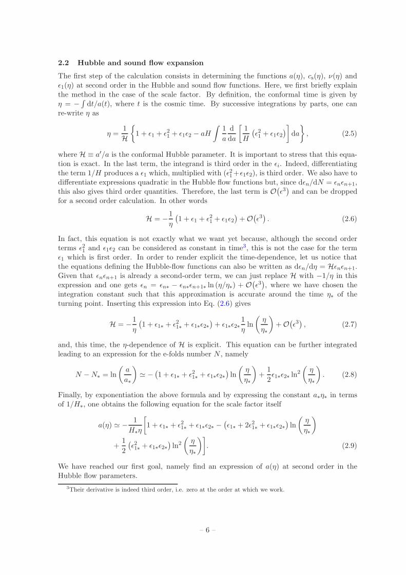
2.2 Hubble and sound flow expansion
The first step of the calculation consists in determining the functions a(η), cs(η), ν(η) andǫ1(η) at second order in the Hubble and sound flow functions. Here, we first briefly explainthe method in the case of the scale factor. By definition, the conformal time is given byη = −
∫
dt/a(t), where t is the cosmic time. By successive integrations by parts, one canre-write η as
η =1
H
{
1 + ǫ1 + ǫ21 + ǫ1ǫ2 − aH
∫
1
a
d
da
[
1
H
(
ǫ21 + ǫ1ǫ2)
]
da
}
, (2.5)
where H ≡ a′/a is the conformal Hubble parameter. It is important to stress that this equa-tion is exact. In the last term, the integrand is third order in the ǫi. Indeed, differentiatingthe term 1/H produces a ǫ1 which, multiplied with (ǫ21+ǫ1ǫ2), is third order. We also have todifferentiate expressions quadratic in the Hubble flow functions but, since dǫn/dN = ǫnǫn+1,this also gives third order quantities. Therefore, the last term is O
(
ǫ3)
and can be droppedfor a second order calculation. In other words
H = −1
η
(
1 + ǫ1 + ǫ21 + ǫ1ǫ2)
+O(
ǫ3)
. (2.6)
In fact, this equation is not exactly what we want yet because, although the second orderterms ǫ21 and ǫ1ǫ2 can be considered as constant in time3, this is not the case for the termǫ1 which is first order. In order to render explicit the time-dependence, let us notice thatthe equations defining the Hubble-flow functions can also be written as dǫn/dη = Hǫnǫn+1.Given that ǫnǫn+1 is already a second-order term, we can just replace H with −1/η in thisexpression and one gets ǫn = ǫn∗ − ǫn∗ǫn+1∗ ln (η/η∗) + O
(
ǫ3)
, where we have chosen theintegration constant such that this approximation is accurate around the time η∗ of theturning point. Inserting this expression into Eq. (2.6) gives
H = −1
η
(
1 + ǫ1∗ + ǫ21∗ + ǫ1∗ǫ2∗)
+ ǫ1∗ǫ2∗1
ηln
(
η
η∗
)
+O(
ǫ3)
, (2.7)
and, this time, the η-dependence of H is explicit. This equation can be further integratedleading to an expression for the e-folds number N , namely
N −N∗ = ln
(
a
a∗
)
≃ −(
1 + ǫ1∗ + ǫ21∗ + ǫ1∗ǫ2∗)
ln
(
η
η∗
)
+1
2ǫ1∗ǫ2∗ ln
2
(
η
η∗
)
. (2.8)
Finally, by exponentiation the above formula and by expressing the constant a∗η∗ in termsof 1/H∗, one obtains the following equation for the scale factor itself
a(η) ≃ − 1
H∗η
[
1 + ǫ1∗ + ǫ21∗ + ǫ1∗ǫ2∗ −(
ǫ1∗ + 2ǫ21∗ + ǫ1∗ǫ2∗)
ln
(
η
η∗
)
+1
2
(
ǫ21∗ + ǫ1∗ǫ2∗)
ln2(
η
η∗
)]
. (2.9)
We have reached our first goal, namely find an expression of a(η) at second order in theHubble flow parameters.
3Their derivative is indeed third order, i.e. zero at the order at which we work.
– 6 –
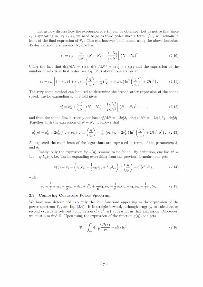
Let us now discuss how the expression of ǫ1(η) can be obtained. Let us notice that sinceǫ1 is appearing in Eq. (2.4), we need to go to third order since a term 1/ǫ1∗ will remain infront of the final expression of Pζ . This can however be obtained using the above formulas.Taylor expanding ǫ1 around N∗ one has
ǫ1 = ǫ1∗ +dǫ1dN
∣
∣
∣
∣
∗
(N −N∗) +1
2
d2ǫ1dN2
∣
∣
∣
∣
∗
(N −N∗)2 + · · · (2.10)
Using the fact that dǫ1/dN = ǫ1ǫ2, d2ǫ1/dN2 = ǫ1ǫ
22 + ǫ1ǫ2ǫ3 and the expression of the
number of e-folds at first order [see Eq. (2.8) above], one arrives at
ǫ1 = ǫ1∗
[
1− ǫ2∗ (1 + ǫ1∗) ln
(
η
η∗
)
+1
2
(
ǫ22∗ + ǫ2∗ǫ3∗)
ln2(
η
η∗
)]
+O(
ǫ4)
. (2.11)
The very same method can be used to determine the second order expression of the soundspeed. Taylor expanding cs in e-fold gives
c2s = c2s∗ +dc2sdN
∣
∣
∣
∣
∗
(N −N∗) +1
2
d2c2sdN2
∣
∣
∣
∣
∗
(N −N∗)2 + · · · , (2.12)
and from the sound flow hierarchy one has dc2s/dN = −2c2s δ1, d2c2s/dN
2 = −2c2s δ1δ2+4c2s δ21 .
Together with the expression of N −N∗, it follows that
c2s (η) = c2s∗ + 2c2s∗(δ1∗ + δ1∗ǫ1∗) ln
(
η
η∗
)
− c2s∗(
δ1∗δ2∗ − 2δ21∗)
ln2(
η
η∗
)
+O(
ǫ3, δ3)
. (2.13)
As expected the coefficients of the logarithms are expressed in terms of the parameters δ1and δ2.
Finally, only the expression for ν(η) remains to be found. By definition, one has ν2 =1/4 + η2U
S(η), i.e. Taylor expanding everything from the previous formulas, one gets
ν(η) = ν∗ −(
ǫ1∗ǫ2∗ +1
2ǫ2∗ǫ3∗ + δ1∗δ2∗
)
ln
(
η
η∗
)
+O(
ǫ3, δ3)
, (2.14)
with
ν∗ ≡3
2+ ǫ1∗ +
1
2ǫ2∗ + δ1∗ + ǫ21∗ +
11
6ǫ1∗ǫ2∗ +
1
6ǫ2∗ǫ3∗ + ǫ1∗δ1∗ +
1
3δ1∗δ2∗. (2.15)
2.3 Comoving Curvature Power Spectrum
We have now determined explicitly the four functions appearing in the expression of thepower spectrum Pζ , see Eq. (2.4). It is straightforward, although lengthy, to calculate, atsecond order, the relevant combination c2s/(a
2νǫ1) appearing in that expression. Moreover,we must also find Ψ. Upon using the expression of the function g(η), one gets
Ψ =
∫ η
η∗
dτ
√
ν2(τ)
τ2− c2s (τ)k
2 . (2.16)
– 7 –
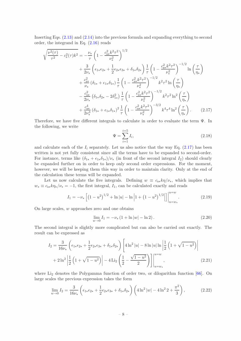
Inserting Eqs. (2.13) and (2.14) into the previous formula and expanding everything to secondorder, the integrand in Eq. (2.16) reads
√
ν2(τ)
τ2− c2s (τ)k
2 = −ν∗τ
(
1− c2s∗k2τ2
ν2∗
)1/2
+3
2ν∗
(
ǫ1∗ǫ2∗ +1
2ǫ2∗ǫ3∗ + δ1∗δ2∗
)
1
τ
(
1− c2s∗k2τ2
ν2∗
)−1/2
ln
(
τ
η∗
)
+c2s∗ν∗
(δ1∗ + ǫ1∗δ1∗)1
τ
(
1− c2s∗k2τ2
ν2∗
)−1/2
k2τ2 ln
(
τ
η∗
)
− c2s∗2ν∗
(
δ1∗δ2∗ − 2δ21∗) 1
τ
(
1− c2s∗k2τ2
ν2∗
)−1/2
k2τ2 ln2(
τ
η∗
)
+c4s∗2ν3∗
(δ1∗ + ǫ1∗δ1∗)2 1
τ
(
1− c2s∗k2τ2
ν2∗
)−3/2
k4τ4 ln2(
τ
η∗
)
. (2.17)
Therefore, we have five different integrals to calculate in order to evaluate the term Ψ. Inthe following, we write
Ψ =i=5∑
i=1
Ii, (2.18)
and calculate each of the Ii separately. Let us also notice that the way Eq. (2.17) has beenwritten is not yet fully consistent since all the terms have to be expanded to second-order.For instance, terms like (δ1∗ + ǫ1∗δ1∗)/ν∗ (in front of the second integral I2) should clearlybe expanded further on in order to keep only second order expressions. For the moment,however, we will be keeping them this way in order to maintain clarity. Only at the end ofthe calculation these terms will be expanded.
Let us now calculate the five integrals. Defining w ≡ cs∗kη/ν∗, which implies thatw∗ ≡ cs∗kη∗/ν∗ = −1, the first integral, I1, can be calculated exactly and reads
I1 = −ν∗
[
(
1− u2)1/2
+ ln |u| − ln∣
∣
∣1 +
(
1− u2)1/2
∣
∣
∣
]
∣
∣
∣
∣
u=w
u=w∗
. (2.19)
On large scales, w approaches zero and one obtains
limw→0
I1 = −ν∗ (1 + ln |w| − ln 2) . (2.20)
The second integral is slightly more complicated but can also be carried out exactly. Theresult can be expressed as
I2 =3
16ν∗
(
ǫ1∗ǫ2∗ +1
2ǫ2∗ǫ3∗ + δ1∗δ2∗
)
[
4 ln2 |u| − 8 ln |u| ln∣
∣
∣
∣
1
2
(
1 +√
1− u2)
∣
∣
∣
∣
+ 2 ln2∣
∣
∣
∣
1
2
(
1 +√
1− u2)
∣
∣
∣
∣
− 4Li2
(
1
2−
√1− u2
2
)]∣
∣
∣
∣
∣
u=w
u=w∗
, (2.21)
where Li2 denotes the Polygamma function of order two, or dilogarithm function [66]. Onlarge scales the previous expression takes the form
limw→0
I2 =3
16ν∗
(
ǫ1∗ǫ2∗ +1
2ǫ2∗ǫ3∗ + δ1∗δ2∗
)(
4 ln2 |w| − 4 ln2 2 +π2
3
)
, (2.22)
– 8 –

where we have used Li2(0) = 0 and Li2(1/2) = π2/12 − (ln2 2)/2. We notice that I1 and I2are logarithmically divergent in the limit w → 0. We will see that this is not a problem andthat those terms cancel out in the final expression of Pζ . This is expected since we knowthat the power spectrum remains constant on larges scales, and as such an exact cancellationof those terms constitutes a consistency check of the method. On the contrary, the integralsI3, I4 and I5 are convergent and can be directly computed. They read
I3 = ν∗ (δ1∗ + ǫ1∗δ1∗) (1− ln 2) , I4 = −ν∗2
(
δ1∗δ2∗ − 2δ21∗)
(
π2
12− 2 + 2 ln 2− ln2 2
)
,
I5 =ν∗2(δ1∗ + ǫ1∗δ1∗)
2
(
2− π2
6− 2 ln 2 + 2 ln2 2
)
. (2.23)
This completes our calculation of the quantity Ψ and we can now evaluate the expres-sion (2.4). Collecting the expressions of a, ǫ1, cs and ν established previously, one getsc2s/(a
2νǫ1) that has to be combined with e2Ψ using the above integrals. After some lengthybut straightforward manipulations, one obtains
Pζ =H2
∗
(
18e−3)
8π2M2Plǫ1∗cs∗
[
1 +
(
−8
3+ 2 ln 2
)
ǫ1∗ +
(
−1
3+ ln 2
)
ǫ2∗ +
(
7
3− ln 2
)
δ1∗
+
(
23
18− 4
3ln 2 +
1
2ln2 2
)
δ21∗ +
(
25
9− π2
24− 7
3ln 2 +
1
2ln2 2
)
δ1∗δ2∗
+
(
−25
9+
13
3ln 2− 2 ln2 2
)
ǫ1∗δ1∗ +
(
13
9− 10
3ln 2 + 2 ln2 2
)
ǫ21∗
+
(
−2
9+
5
3ln 2− ln2 2
)
ǫ2∗δ1∗ +
(
−25
9+
π2
12+
1
3ln 2 + ln2 2
)
ǫ1∗ǫ2∗
+
(
− 1
18− 1
3ln 2 +
1
2ln2 2
)
ǫ22∗ +
(
−1
9+
π2
24+
1
3ln 2− 1
2ln2 2
)
ǫ2∗ǫ3∗
]
.
(2.24)
Several remarks are in order at this stage. Firstly, in the above calculation, we haveassumed that the initial state of the perturbations is the Bunch-Davies vacuum. This impliesthat |Bk|2 = π/2. Notice that, in the context of k-inflation, this is a non-trivial choicesince, as discussed in Ref. [59], the time dependence of the sound speed could be such thatthe adiabatic regime is not available anymore4. In this paper, we assume that this doesnot occur and that the function cs(η) is initially smooth enough. Secondly, as announcedabove, all the time-dependent terms ln |w| have canceled out and the expression of Pζ istime-independent. Thirdly, Eq. (2.24) should be compared with Eq. (51) of Ref. [59]. Thesetwo expressions coincide at first order, which is another indication that the above formula forPζ is correct. Fourthly, in the overall amplitude, we notice the presence of the factor 18 e−3.As explained in Refs. [48] and [59], this is typical in a approximation scheme based on theWKB method or its extension (such as the uniform approximation). This leads to a ≃ 10%error in the estimation of the amplitude. In Refs. [53, 54], it was shown that, by taking intoaccount higher order terms in the adiabatic expansion, this shortcomings can easily be fixed.In that case, one obtains a new overall coefficient which dramatically reduces the error in the
4Let us notice however that one can still re-define a new time variable to absorb the cs-dependence in themode equation [42]. In terms of that new time variable, one could always set Bunch-Davies initial conditionsfor the scalar, but this would not be compatible with those of the tensor modes.
– 9 –
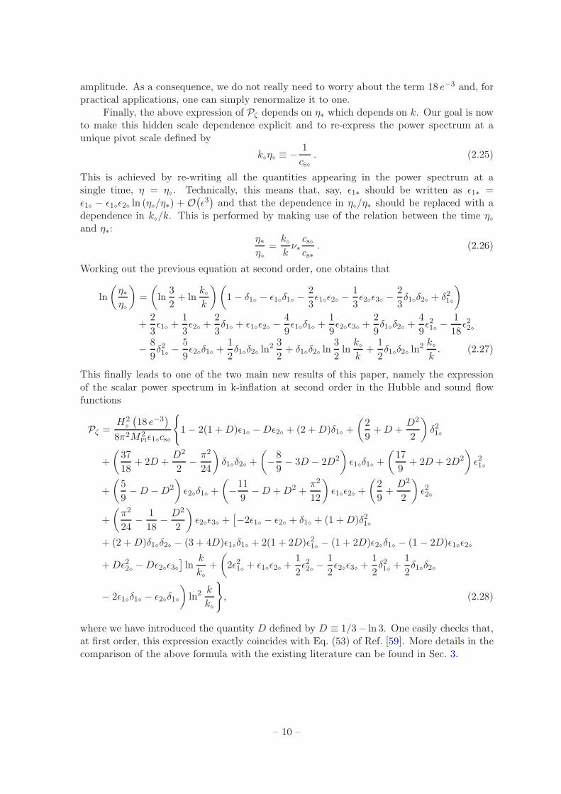
amplitude. As a consequence, we do not really need to worry about the term 18 e−3 and, forpractical applications, one can simply renormalize it to one.
Finally, the above expression of Pζ depends on η∗ which depends on k. Our goal is nowto make this hidden scale dependence explicit and to re-express the power spectrum at aunique pivot scale defined by
k⋄η⋄≡ − 1
cs⋄. (2.25)
This is achieved by re-writing all the quantities appearing in the power spectrum at asingle time, η = η
⋄. Technically, this means that, say, ǫ1∗ should be written as ǫ1∗ =
ǫ1⋄ − ǫ1⋄ǫ2⋄ ln (η⋄/η∗) + O
(
ǫ3)
and that the dependence in η⋄/η∗ should be replaced with a
dependence in k⋄/k. This is performed by making use of the relation between the time η
⋄
and η∗:η∗η⋄
=k⋄
kν∗
cs⋄cs∗
. (2.26)
Working out the previous equation at second order, one obtains that
ln
(
η∗η⋄
)
=
(
ln3
2+ ln
k⋄
k
)(
1− δ1⋄ − ǫ1⋄δ1⋄ −2
3ǫ1⋄ǫ2⋄ −
1
3ǫ2⋄ǫ3⋄ −
2
3δ1⋄δ2⋄ + δ21⋄
)
+2
3ǫ1⋄ +
1
3ǫ2⋄ +
2
3δ1⋄ + ǫ1⋄ǫ2⋄ −
4
9ǫ1⋄δ1⋄ +
1
9ǫ2⋄ǫ3⋄ +
2
9δ1⋄δ2⋄ +
4
9ǫ21⋄ −
1
18ǫ22⋄
− 8
9δ21⋄ −
5
9ǫ2⋄δ1⋄ +
1
2δ1⋄δ2⋄ ln
2 3
2+ δ1⋄δ2⋄ ln
3
2ln
k⋄
k+
1
2δ1⋄δ2⋄ ln
2 k⋄
k. (2.27)
This finally leads to one of the two main new results of this paper, namely the expressionof the scalar power spectrum in k-inflation at second order in the Hubble and sound flowfunctions
Pζ =H2
⋄
(
18 e−3)
8π2M2Plǫ1⋄cs⋄
{
1− 2(1 +D)ǫ1⋄ −Dǫ2⋄ + (2 +D)δ1⋄ +
(
2
9+D +
D2
2
)
δ21⋄
+
(
37
18+ 2D +
D2
2− π2
24
)
δ1⋄δ2⋄ +
(
−8
9− 3D − 2D2
)
ǫ1⋄δ1⋄ +
(
17
9+ 2D + 2D2
)
ǫ21⋄
+
(
5
9−D −D2
)
ǫ2⋄δ1⋄ +
(
−11
9−D +D2 +
π2
12
)
ǫ1⋄ǫ2⋄ +
(
2
9+
D2
2
)
ǫ22⋄
+
(
π2
24− 1
18− D2
2
)
ǫ2⋄ǫ3⋄ +[
−2ǫ1⋄ − ǫ2⋄ + δ1⋄ + (1 +D)δ21⋄
+ (2 +D)δ1⋄δ2⋄ − (3 + 4D)ǫ1⋄δ1⋄ + 2(1 + 2D)ǫ21⋄ − (1 + 2D)ǫ2⋄δ1⋄ − (1− 2D)ǫ1⋄ǫ2⋄
+Dǫ22⋄ −Dǫ2⋄ǫ3⋄]
lnk
k⋄
+
(
2ǫ21⋄ + ǫ1⋄ǫ2⋄ +1
2ǫ22⋄ −
1
2ǫ2⋄ǫ3⋄ +
1
2δ21⋄ +
1
2δ1⋄δ2⋄
− 2ǫ1⋄δ1⋄ − ǫ2⋄δ1⋄
)
ln2k
k⋄
}
, (2.28)
where we have introduced the quantity D defined by D ≡ 1/3− ln 3. One easily checks that,at first order, this expression exactly coincides with Eq. (53) of Ref. [59]. More details in thecomparison of the above formula with the existing literature can be found in Sec. 3.
– 10 –
Using the method of Ref. [67], one can also deduce the expression of the scalar spectralindex which reads
nS − 1 = −2ǫ1⋄ − ǫ2⋄ + δ1⋄ − 2ǫ21⋄ − (2D + 3) ǫ1⋄ǫ2⋄ + 3ǫ1⋄δ1⋄ + ǫ2⋄δ1⋄ −Dǫ2⋄ǫ3⋄
− δ21⋄ + (D + 2) δ1⋄δ2⋄ − 2ǫ31⋄ −(
47
9+ 6D
)
ǫ21⋄ǫ2⋄ + 5ǫ21⋄δ1⋄
+
(
−20
9− 3D −D2 +
π2
12
)
ǫ1⋄ǫ22⋄ +
(
−11
9− 4D −D2 +
π2
12
)
ǫ1⋄ǫ2⋄ǫ3⋄
+
(
73
9+ 5D
)
δ1⋄ǫ1⋄ǫ2⋄ − 4ǫ1⋄δ21⋄ +
(
46
9+ 4D
)
ǫ1⋄δ1⋄δ2⋄ +4
9ǫ22⋄ǫ3⋄
+
(
− 1
18− D2
2+
π2
24
)
ǫ2⋄ǫ23⋄ +
(
5
9+ 2D
)
δ1⋄ǫ2⋄ǫ3⋄
+
(
− 1
18− D2
2+
π2
24
)
ǫ2⋄ǫ3⋄ǫ4⋄ − δ21⋄ǫ2⋄ +
(
5
9+D
)
δ1⋄δ2⋄ǫ2⋄ + δ31⋄
−(
50
9+ 3D
)
δ21⋄δ2⋄ +
(
37
18+ 2D +
D2
2− π2
24
)
δ1⋄δ22⋄
+
(
37
18+ 2D +
D2
2− π2
24
)
δ1⋄δ2⋄δ3⋄ (2.29)
At first order in the flow parameters, one recovers the standard expression, i.e. nS − 1 =−2ǫ1⋄ − ǫ2⋄ + δ1⋄. One can also check that the second order corrections are similar to thosefound in Ref. [59]. Here, for the first time, we have given the formula of the spectral index atthird order. This is of course possible only because we have determined the overall amplitudeat second order. This also allows us to determine the higher order corrections to the runningand to the running of the running. For instance, one can calculate αS at the fourth orderand the running of the running at the fifth order. Here, in order to illustrate the efficiencyof the method, we just present the expression of αS. It reads
αS = −2ǫ1⋄ǫ2⋄ − ǫ2⋄ǫ3⋄ + δ1⋄δ2⋄ − 6ǫ21⋄ǫ2⋄ − (3 + 2D) ǫ1⋄ǫ22⋄ − (4 + 2D) ǫ1⋄ǫ2⋄ǫ3⋄ + 5ǫ1⋄ǫ2⋄δ1⋄
+ 4ǫ1⋄δ1⋄δ2⋄ −Dǫ2⋄ǫ23⋄ −Dǫ2⋄ǫ3⋄ǫ4⋄ + 2δ1⋄ǫ2⋄ǫ3⋄ + δ1⋄δ2⋄ǫ2⋄ − 3δ21⋄δ2⋄ + (2 +D) δ1⋄δ
22⋄
+ (2 +D) δ1⋄δ2⋄δ3⋄ − 12ǫ31⋄ǫ2⋄ −(
139
9+ 14D
)
ǫ21⋄ǫ22⋄ −
(
83
9+ 8D
)
ǫ21⋄ǫ2⋄ǫ3⋄
+ 21δ1⋄ǫ21⋄ǫ2⋄ + 9δ1⋄δ2⋄ǫ
21⋄ +
(
−20
9− 3D −D2 +
π2
12
)
ǫ1⋄ǫ32⋄
+
(
−20
3− 10D − 3D2 +
π2
4
)
ǫ1⋄ǫ22⋄ǫ2⋄ +
(
100
9+ 7D
)
δ1⋄ǫ1⋄ǫ22⋄
+
(
−11
9− 5D −D2 +
π2
12
)
ǫ1⋄ǫ2⋄ǫ23⋄ +
(
−11
9− 5D −D2 +
π2
12
)
ǫ1⋄ǫ2⋄ǫ3⋄ǫ4⋄
+
(
127
9+ 7D
)
δ1⋄ǫ1⋄ǫ2⋄ǫ3⋄ − 9δ21⋄ǫ1⋄ǫ2⋄ +
(
137
9+ 9D
)
δ1⋄δ2⋄ǫ1⋄ǫ2⋄ − 15δ21⋄δ2⋄ǫ1⋄
+
(
64
9+ 5D
)
ǫ1⋄δ1⋄δ22⋄ +
(
64
9+ 5D
)
ǫ1⋄δ1⋄δ2⋄δ3⋄ +8
9ǫ22⋄ǫ
23⋄ +
4
9ǫ22⋄ǫ3⋄ǫ4⋄
+
(
− 1
18− D2
2+
π2
24
)
ǫ2⋄ǫ33⋄ +
(
−1
6− 3D2
2+
π2
8
)
ǫ2⋄ǫ23⋄ǫ4⋄ +
(
5
9+ 3D
)
δ1⋄ǫ2⋄ǫ23⋄
– 11 –
+
(
− 1
18− D2
2+
π2
24
)
ǫ2⋄ǫ3⋄ǫ24⋄ +
(
− 1
18− D2
2+
π2
24
)
ǫ2⋄ǫ3⋄ǫ4⋄ǫ5⋄
+
(
5
9+ 3D
)
δ1⋄ǫ2⋄ǫ3⋄ǫ4⋄ − 3δ21⋄ǫ2⋄ǫ3⋄ +
(
10
9+ 3D
)
δ1⋄δ2⋄ǫ2⋄ǫ3⋄ − 3δ21⋄δ2⋄ǫ2⋄
+
(
5
9+D
)
δ1⋄δ22⋄ǫ2⋄ +
(
5
9+D
)
δ1⋄δ2⋄δ3⋄ǫ2⋄ + 6δ31⋄δ2⋄ −(
118
9+ 7D
)
δ21⋄δ22⋄
−(
68
9+ 4D
)
δ21⋄δ2⋄δ3⋄ +
(
37
18+ 2D +
D2
2− π2
24
)
δ1⋄δ32⋄
+
(
37
6+ 6D +
3D2
2− π2
8
)
δ1⋄δ22⋄δ3⋄ +
(
37
18+ 2D +
D2
2− π2
24
)
δ1⋄δ2⋄δ23⋄
+
(
37
18+ 2D +
D2
2− π2
24
)
δ1⋄δ2⋄δ3⋄δ4⋄ (2.30)
One can check that the second and third order corrections match the expression alreadyfound in Ref. [59]. The fourth order corrections represent a new result.
2.4 Tensor Power Spectrum
In this section, we repeat the previous analysis but for tensor perturbations. Since themethod is the same and, fortunately, the calculations are easier, the details will be skipped.The main difference between gravity waves and density perturbations is that their effectivepotential is not the same, see Eqs. (1.4) and (1.6). This implies that the function ν(η) fortensors is different from the one of the scalars. One gets for the tensor
ν2(η) =9
4+ 3ǫ1∗ + 4ǫ21∗ + 4ǫ1∗ǫ2∗ − 3ǫ1∗ǫ2∗ ln
(
η
η∗
)
+O(
ǫ3)
. (2.31)
As a consequence, the functions g(η), f(η), and hence Ψ, are also different. Using the uniformapproximation to evaluate µk and inserting the corresponding formula into the expression ofPh given by Eq. (1.9), one obtains
Ph =2(
18 e−3)
H2∗
π2M2Pl
[
1 +
(
−8
3+ 2 ln 2
)
ǫ1∗ +
(
π2
12− 26
9+
8
3ln 2− ln2 2
)
ǫ1∗ǫ2∗
+
(
13
9− 10
3ln 2 + 2 ln2 2
)
ǫ21∗
]
. (2.32)
This equation is for the tensors what Eq. (2.24) is for the scalars. As explained before, onehas still to make explicit the scale dependence hidden in η∗. In the case of tensors, the pivotpoint is usually defined by k⋆η⋆ = −1 since gravity waves propagate at the speed of light.This leads to the following expression for the power spectrum
Ph =2(
18 e−3)
H2⋆
π2M2Pl
{
1− 2(1 +D)ǫ1⋆ +
(
17
9+ 2D + 2D2
)
ǫ21⋆ +
(
−19
9+
π2
12
− 2D −D2
)
ǫ1⋆ǫ2⋆ +[
−2ǫ1⋆ + 2(1 + 2D)ǫ21⋆ − 2(1 +D)ǫ1⋆ǫ2⋆]
lnk⋆k
+(
2ǫ21⋆ − ǫ1⋆ǫ2⋆)
ln2k⋆k
}
. (2.33)
– 12 –
Let us notice that, in order to obtain this relationship, we have used the initial conditions forgravity waves |Bk| = 1/M2
Pl. Otherwise, one notices the presence of the WKB factor 18 e3
and one can check that, at first order, it coincides with the known expression for the tensorpower spectrum. The above formula, being expressed at the time η⋆, is convenient for SFMKmodels only, but not for k-inflation. Indeed, all parameters here are functions evaluated atthe time η⋆ which is different that the one at which the scalar power spectrum is calculated,namely η
⋄. It has become a common mistake to try fitting data with both Eq. (2.28) and
Eq.(2.33) while implicitly assuming that all Hubble and sound flow “parameters” are thesame. As we have explicitly shown before, they do differ and such a fit would absolutelymake no sense.
However, within slow-roll, one can re-express the tensor power spectrum at the samepivot point as for the scalar power spectrum. As before, each quantity in the tensor powerspectrum should be re-expressed at the scalar pivot point, as for instance ǫ1⋆ = ǫ1⋄ −ǫ1⋄ǫ2⋄ ln cs⋄ + O
(
ǫ3, δ3)
. The quantity cs⋄ appears because it is present in the ratio of thetensor to scalar pivot points. It follows that the final expression for the tensor power spec-trum for k-inflation is
Ph =2(
18e−3)
H2⋄
π2M2Pl
{
1− 2(1 +D − ln cs⋄)ǫ1⋄ +
[
17
9+ 2D + 2D2 + 2 ln2 cs⋄
− 2(1 + 2D) ln cs⋄
]
ǫ21⋄ +
[
−19
9+
π2
12− 2D −D2 + 2(1 +D) ln cs⋄ − ln2 cs⋄
]
ǫ1⋄ǫ2⋄
+
[
−2ǫ1⋄ + (2 + 4D − 4 ln cs⋄)ǫ21⋄ + (−2− 2D + 2 ln cs⋄)ǫ1⋄ǫ2⋄
]
lnk⋄
k
+(
2ǫ21⋄ − ǫ1⋄ǫ2⋄)
ln2k⋄
k
}
, (2.34)
where now “diamonded” terms are evaluated at the scalar pivot point. This new formula isthe second main result of the present paper. It extends to second order the results of Ref. [59].As for the scalar modes, this expression also allows us to calculate the tensor spectral indexat third order. One obtains
nT = −2ǫ1⋄ − 2ǫ21⋄ + (−2− 2D + 2 ln cs⋄) ǫ1⋄ǫ2⋄ − 2ǫ31⋄ +
(
−38
9− 6D + 6 ln cs⋄
)
ǫ21⋄ǫ2⋄
+
(
−19
9− 2D −D2 +
π2
12+ 2 ln cs⋄ + 2D ln cs⋄ − ln2 cs⋄
)
ǫ1⋄ǫ22⋄
+
(
−19
9− 2D −D2 +
π2
12+ 2 ln cs⋄ + 2D ln cs⋄ − ln2 cs⋄
)
ǫ1⋄ǫ2⋄ǫ3⋄ (2.35)
Of course, at first order, one recovers the standard formula, nT = −2ǫ1⋄. We have alreadydiscussed before the relevance of higher order corrections for Bayesian parameter estimation.Notice that, in the case of primordial gravitational waves and as discussed in Ref. [68],another motivation is the possibility of detecting them directly. Indeed, in that case, oneneeds to estimate their power spectrum today and, due to the very large lever arm betweenthe cosmological scales and the smaller scales where a direct detection can be performed, itis necessay to calculate the power spectrum at the end of inflation very precisely. In thiscontext, higher order corrections become mandatory. Similarly, the running of the tensors is
– 13 –
obtained at fourth order and reads
αT = −2ǫ1⋄ǫ2⋄ − 6ǫ21⋄ǫ2⋄ + (−2− 2D + 2 ln cs⋄)ǫ1⋄ǫ22⋄ + (−2− 2D + 2 ln cs⋄)ǫ1⋄ǫ2⋄ǫ3⋄
− 12ǫ31⋄ǫ2⋄ +
(
−112
9− 14D + 14 ln cs⋄
)
ǫ21⋄ǫ22⋄ +
(
−56
9− 8D + 8 ln cs⋄
)
ǫ21⋄ǫ2⋄ǫ3⋄
+
[
−19
9− 2D −D2 +
π2
12+ 2(1 +D) ln cs⋄ − ln2 cs⋄
]
(
ǫ1⋄ǫ32⋄ + 3ǫ1⋄ǫ
22⋄ǫ3⋄
+ǫ1⋄ǫ2⋄ǫ23⋄ + ǫ1⋄ǫ2⋄ǫ3⋄ǫ4⋄
)
. (2.36)
Finally, one can also deduce the tensor to scalar ratio at the third order. It reads
r = 16ǫ1⋄cs⋄
[
1 + 2ǫ1⋄ ln cs⋄ +Dǫ2⋄ − (2 +D) δ1⋄ +
(
34
9+ 3D +
D2
2
)
δ21⋄
+
(
−37
18− 2D − D2
2+
π2
24
)
δ1⋄δ2⋄ −(
5
9+ 3D +D2
)
δ1⋄ǫ2⋄ +
(
−2
9+
D2
2
)
ǫ22⋄
+1
72
(
4 + 36D2 − 3π2)
ǫ2⋄ǫ3⋄ + 2ǫ21⋄ (1 + ln cs⋄) ln cs⋄
+
(
−28
9− 3D − 4 ln cs⋄ − 2D ln cs⋄
)
δ1⋄ǫ1⋄
+
(
−8
9+D + 2 ln cs⋄ + 4D ln cs⋄ − ln2 cs⋄
)
ǫ1⋄ǫ2⋄
]
. (2.37)
As usual the leading term is proportional to ǫ1⋄cs⋄ and the above formula shows that thecorresponding corrections depend on the flow parameters but also on the sound speed.
3 Discussion and Conclusions
The power spectra of Eqs. (2.28) and (2.34) represent the main result of this article. Thereare the first calculation, at second order in the Hubble and sound flow functions, of the scalarand tensor power spectra in k-inflation within the uniform approximation. In this section, wediscuss our results and check their consistency. In particular, in some limits, our calculationshould reproduce known results already derived in the literature. As we show below, this isindeed the case.
We have seen before that the power spectrum is obtained as an expansion around thepivot scale and that the most general expression of Pζ can be written as
Pζ(k) = Pζ(k⋄)∑
n≥0
ann!
lnnk
k⋄
, (3.1)
where Pζ is the overall amplitude and the coefficients an are functions of the horizon flowparameters. The expression of an always starts at order n, i.e. a0 starts with one, a1starts with a term of order O(ǫ, δ), a2 with a term of order O
(
ǫ2, δ2, ǫδ)
and so on. Asalready mentioned before, k-inflationary power spectra were determined at first order inRef. [59]. This means that the expression found in that paper included only the first twoterms, proportional to a0 and a1. There is however a trick derived in Ref. [67] which allowsus to determine some higher order terms. Indeed, the power spectrum should not depend
– 14 –
on the choice of the pivot scale, which is arbitrary. As a consequence, one can establish thefollowing recursion relation
an+1 =d ln Pζ
d ln k⋄
an +dan
d ln k⋄
. (3.2)
Given that a0 was given at first order in Ref. [59], it was then possible to calculate a1 up tosecond order and a2 to third order [see Eqs. (64) and (65) in that reference]. Therefore, onecan compare those formulas to the expression obtained in this article. One finds that theyare the same, indicating the consistency of our results.
Another way to verify the validity of our expressions is to take the limit cs = 1 and tocompare the resulting formulas to the results already obtained in the literature for SFMKmodels. As mentioned in the introduction, second order results were first obtained usingthe Green function method in Ref. [47]. The corresponding expression for the scalar powerspectrum reads
Pζ =H2
8π2M2Plǫ1
{
1− 2(C + 1)ǫ1 − Cǫ2 +
(
2C2 + 2C +π2
2− 5
)
ǫ21
+
(
C2 − C +7π2
12− 7
)
ǫ1ǫ2 +
(
C2
2+
π2
8− 1
)
ǫ22 +
(
−C2
2+
π2
24
)
ǫ2ǫ3
+[
−2ǫ1 − ǫ2 + 2(2C + 1)ǫ21 + (2C − 1)ǫ1ǫ2 +Cǫ22 − Cǫ2ǫ3]
lnk
k⊛
+
(
2ǫ21 + ǫ2ǫ2 +1
2ǫ22 −
1
2ǫ2ǫ3
)
ln2k
k⊛
}
, (3.3)
where the constant C is defined by C ≡ γ + ln 2− 2 ≃ −0.7296, γ being the Euler constant,while the expression of the gravity wave power spectrum can be written as
Ph =2H2
π2M2Pl
{
1− 2(C + 1)ǫ1 +
(
2C2 + 2C +π2
2− 5
)
ǫ21 +
(
−C2 − 2C +π2
12− 2
)
ǫ1ǫ2
+[
−2ǫ1 + 2(2C + 1)ǫ21 − 2(C + 1)ǫ1ǫ2]
lnk
k⊛
+
(
2ǫ21 − ǫ1ǫ2
)
ln2k
k⊛
}
. (3.4)
In the two previous formulas (3.3) and (3.4), the Hubble flow functions are evaluated attime η⊛ such that a(η⊛)H(η⊛) = k⊛ which slightly differs from the time k
⋄η⋄= −1 (for
cs⋄ = 1) used in the present paper. Therefore, if we want to compare Eqs. (2.28) and (2.34)with cs⋄ = 1 to Eqs. (3.3) and (3.4), one should first re-express the latter in terms of theHubble flow parameters evaluated at time k
⋄η⋄= −1. In the following, in order to simplify
the discussion, we focus only on the scalar case but the tensor case could be treated in thesame manner. From the definition of η⊛ one has η⊛/η⋄
= 1 + ǫ1⋄ + ǫ21⋄ + ǫ1⋄ǫ2⋄ +O(
ǫ3)
. Asconsequence, in Eqs. (3.3) and (3.4), one should just replace ǫ1, ǫ2 with ǫ1⋄, ǫ2⋄ and H2/ǫ1
– 15 –

with H2⋄/ǫ1⋄(1 + 2ǫ21⋄ + ǫ1⋄ǫ2⋄). This yields the following expression
Pζ =H2
⋄
8π2M2Plǫ1⋄
{
1− 2(C + 1)ǫ1⋄ − Cǫ2⋄ +
(
2C2 + 2C +π2
2− 3
)
ǫ21⋄
+
(
C2 − C +7π2
12− 6
)
ǫ1⋄ǫ2⋄ +
(
C2
2+
π2
8− 1
)
ǫ22⋄ +
(
−C2
2+
π2
24
)
ǫ2⋄ǫ3⋄
+[
−2ǫ1⋄ − ǫ2⋄ + 2(2C + 1)ǫ21⋄ + (2C − 1)ǫ1⋄ǫ2⋄ + Cǫ22⋄ − Cǫ2⋄ǫ3⋄]
lnk
k⋄
+
(
2ǫ21⋄ + ǫ1⋄ǫ2⋄ +1
2ǫ22⋄ −
1
2ǫ2⋄ǫ3⋄
)
ln2k
k⋄
}
, (3.5)
that can be now compared to Eq. (2.28). As already discussed, the overall amplitude differs bythe WKB factor 18 e−3. We also notice that the terms in D in Eq. (2.28) exactly correspondsto the term in C in Eq. (3.5). For instance, the coefficient of ǫ21⋄ in Eq. (2.28) contains a term2D2+2D while the coefficient of ǫ21⋄ in Eq. (3.5) contains a 2C2+2C. One easily checks thatthis is the rule for all first and second order terms. Provided one substitutes D with C, thefirst order term in the amplitude, the coefficient of ln k/k
⋄and the coefficient of ln2(k/k
⋄)
are identical. The only difference appears in the second order terms in the amplitude. Forinstance, the coefficients of ǫ21⋄ in Eq. (2.28) is 2D2+2D+17/9 while it is 2C2+2C+π2/2−3in Eq. (3.5). But 17/9 ≃ 1.88 and π2/2 − 3 ≃ 1.93 and, therefore, the two terms are in factnumerically very close. The same is true for all the other terms in the amplitude. Therefore,we conclude that our result (2.28), specialized to SFMK models, is fully consistent withEq. (3.5) that comes from another approximation scheme. This confirms its validity.
Let us now compare our result to the one of Refs. [53, 54] calculated with the help ofthe WKB approximation. The scalar power spectrum obtained in those articles reads
Pζ =H2
8π2M2Plǫ1
AWKB
{
1− 2(DWKB
+ 1)ǫ1 −DWKB
ǫ2 +
(
2D2
WKB+ 2D
WKB− 1
9
)
ǫ21
+
(
D2
WKB−D
WKB+
π2
12− 20
9
)
ǫ1ǫ2 +
(
D2
WKB
2+
2
9
)
ǫ22 +
(
−D2
WKB
2+
π2
24− 1
18
)
ǫ2ǫ3
+[
−2ǫ1 − ǫ2 + 2(2DWKB
+ 1)ǫ21 + (2DWKB
− 1)ǫ1ǫ2 +DWKB
ǫ22 −DWKB
ǫ2ǫ3]
lnk
k⊛
+
(
2ǫ21 + ǫ1ǫ2 +1
2ǫ22 −
1
2ǫ2ǫ3
)
ln2k
k⊛
}
, (3.6)
while the tensor power spectrum is given by the following formula
Ph =2H2
π2M2Pl
AWKB
{
1− 2(DWKB
+ 1)ǫ1 +
(
2D2
WKB+ 2D
WKB− 1
9
)
ǫ21 +
(
−D2
WKB− 2D
WKB
+π2
12− 19
9
)
ǫ1ǫ2 +[
−2ǫ1 + 2(2DWKB
+ 1)ǫ21 − 2(DWKB
+ 1)ǫ1ǫ2]
lnk
k⊛
+(
2ǫ21 − ǫ1ǫ2)
ln2k
k⊛
}
. (3.7)
– 16 –

In these equations, AWKB
= 18 e−3 and DWKB
= 1/3 − ln 3, that is to say exactly whatwas found by means of the uniform approximation as D
WKB= D. As already mentioned,
Refs. [53, 54] have shown that, by taking the next order in the adiabatic approximationinto account, one obtains a new value for these two constants (in some sense, they arerenormalized), namely A
WKBbecomes 361/(18 e3) ≃ 0.99 and D
WKB= 7/19−ln 3 ≃ −0.7302.
In particular, the new value of DWKB
is closer to the constant C than the non-renormalizedone. Both Eqs. (3.6) and (3.7) are evaluated at the pivot time η⊛ and have to be time-shiftedto η
⋄to be compared with our results. Proceeding as previously, it is easy to show that this
modifies the coefficients of ǫ21 which now becomes 2D2
WKB+2D
WKB+17/9, and the coefficient
of ǫ1ǫ2 which becomes 2D2
WKB−D
WKB+π2/12−11/9. In other words Eqs. (2.28) and Eq. (3.6)
expressed at η⋄are exactly the same for cs⋄ = 1. This is maybe not so surprising considering
the fact that the WKB and uniform approximations are closely related methods.A few words are in order about Ref. [55]. Historically, this is probably the first paper that
attempted to evaluate the k-inflationary power spectrum at second order in some equivalentof the Hubble and sound flow functions used here. The method chosen is the Green functionexpansion discussed before. However, a specific form for the sound speed, which in thelanguage of the present paper would be a first order approximation of c2s , was also postulated.Together with a k−dependence kept implicit, this makes the comparison with the presentwork difficult. For this reason, we do not investigate further this issue.
To conclude, let us briefly recap our main result and discuss directions for future works.In this paper, using the uniform approximation, we have calculated the scalar and tensorpower spectra in k-inflation, at second order in the Hubble and sound flow parameters, seeEqs. (2.28) and (2.34). We have carefully checked that, in the various limits where ourcalculation reduces to known cases, consistent results are obtained. The next step is clearlyto use these power spectra in order to constrain the values of the Hubble and sound flowparameters using CMB observations. This was done in Ref. [62] but only for the first orderpower spectra (since only this result was available at that time). Given the on-going fluxof high precision data, such as those from the Planck satellite, the results obtained in thisarticle should be important to keep theoretical uncertainties at a minimal level. In this way,as discussed in the introduction, one may hope to obtain unprecedented information on theinflationary scenario.
References
[1] A. A. Starobinsky, A New Type of Isotropic Cosmological Models Without Singularity,Phys.Lett. B91 (1980) 99–102.
[2] A. H. Guth, The Inflationary Universe: A Possible Solution to the Horizon and FlatnessProblems, Phys. Rev. D23 (1981) 347–356.
[3] P. Peter and J.-P. Uzan, Primordial cosmology. Oxford University Press, UK, 2013.
[4] J. Martin, Inflation and precision cosmology, Braz. J. Phys. 34 (2004) 1307–1321,[astro-ph/0312492].
[5] J. Martin, Inflationary cosmological perturbations of quantum- mechanical origin, Lect. NotesPhys. 669 (2005) 199–244, [hep-th/0406011].
[6] J. Martin, Inflationary perturbations: The cosmological Schwinger effect, Lect. Notes Phys. 738(2008) 193–241, [arXiv:0704.3540].
[7] L. Sriramkumar, An introduction to inflation and cosmological perturbation theory,arXiv:0904.4584.
– 17 –
[8] Supernova Search Team Collaboration, J. L. Tonry et al., Cosmological results from high-zsupernovae, Astrophys.J. 594 (2003) 1–24, [astro-ph/0305008].
[9] Supernova Search Team Collaboration, A. G. Riess et al., Type Ia supernova discoveries atz > 1 from the Hubble Space Telescope: Evidence for past deceleration and constraints on darkenergy evolution, Astrophys.J. 607 (2004) 665–687, [astro-ph/0402512].
[10] A. G. Riess, L.-G. Strolger, S. Casertano, H. C. Ferguson, B. Mobasher, et al., New HubbleSpace Telescope Discoveries of Type Ia Supernovae at z¿1: Narrowing Constraints on the EarlyBehavior of Dark Energy, Astrophys.J. 659 (2007) 98–121, [astro-ph/0611572].
[11] SDSS Collaboration Collaboration, J. K. Adelman-McCarthy et al., The Sixth Data Releaseof the Sloan Digital Sky Survey, Astrophys.J.Suppl. 175 (2008) 297–313, [arXiv:0707.3413].
[12] SDSS Collaboration Collaboration, K. N. Abazajian et al., The Seventh Data Release of theSloan Digital Sky Survey, Astrophys.J.Suppl. 182 (2009) 543–558, [arXiv:0812.0649].
[13] D. Larson, J. Dunkley, G. Hinshaw, E. Komatsu, M. Nolta, et al., Seven-Year WilkinsonMicrowave Anisotropy Probe (WMAP) Observations: Power Spectra and WMAP-DerivedParameters, Astrophys.J.Suppl. 192 (2011) 16, [arXiv:1001.4635].
[14] WMAP Collaboration Collaboration, E. Komatsu et al., Seven-Year Wilkinson MicrowaveAnisotropy Probe (WMAP) Observations: Cosmological Interpretation, Astrophys.J.Suppl. 192(2011) 18, [arXiv:1001.4538].
[15] A. G. Riess, L. Macri, S. Casertano, H. Lampeitl, H. C. Ferguson, et al., A 3Telescope andWide Field Camera 3, Astrophys.J. 730 (2011) 119, [arXiv:1103.2976].
[16] G. Hinshaw, D. Larson, E. Komatsu, D. Spergel, C. Bennett, et al., Nine-Year WilkinsonMicrowave Anisotropy Probe (WMAP) Observations: Cosmological Parameter Results,arXiv:1212.5226.
[17] C. Bennett, D. Larson, J. Weiland, N. Jarosik, G. Hinshaw, et al., Nine-Year WilkinsonMicrowave Anisotropy Probe (WMAP) Observations: Final Maps and Results,arXiv:1212.5225.
[18] Z. Hou, C. Reichardt, K. Story, B. Follin, R. Keisler, et al., Constraints on Cosmology from theCosmic Microwave Background Power Spectrum of the 2500-square degree SPT-SZ Survey,arXiv:1212.6267.
[19] K. Story, C. Reichardt, Z. Hou, R. Keisler, K. Aird, et al., A Measurement of the CosmicMicrowave Background Damping Tail from the 2500-square-degree SPT-SZ survey,arXiv:1210.7231.
[20] J. L. Sievers, R. A. Hlozek, M. R. Nolta, V. Acquaviva, G. E. Addison, et al., The AtacamaCosmology Telescope: Cosmological parameters from three seasons of data, arXiv:1301.0824.
[21] J. Dunkley, E. Calabrese, J. Sievers, G. Addison, N. Battaglia, et al., The Atacama CosmologyTelescope: likelihood for small-scale CMB data, arXiv:1301.0776.
[22] J.-M. Lamarre, J.-L. Puget, P. A. R. Ade, F. Bouchet, G. Guyot, A. E. Lange, F. Pajot,A. Arondel, K. Benabed, J.-L. Beney, A. Benoıt, J.-P. Bernard, R. Bhatia, Y. Blanc, J. J.Bock, E. Breelle, T. W. Bradshaw, P. Camus, A. Catalano, J. Charra, M. Charra, S. E. Church,F. Couchot, A. Coulais, B. P. Crill, M. R. Crook, K. Dassas, P. de Bernardis, J. Delabrouille,P. de Marcillac, J.-M. Delouis, F.-X. Desert, C. Dumesnil, X. Dupac, G. Efstathiou, P. Eng,C. Evesque, J.-J. Fourmond, K. Ganga, M. Giard, R. Gispert, L. Guglielmi, J. Haissinski,S. Henrot-Versille, E. Hivon, W. A. Holmes, W. C. Jones, T. C. Koch, H. Lagardere, P. Lami,J. Lande, B. Leriche, C. Leroy, Y. Longval, J. F. Macıas-Perez, T. Maciaszek, B. Maffei,B. Mansoux, C. Marty, S. Masi, C. Mercier, M.-A. Miville-Deschenes, A. Moneti, L. Montier,J. A. Murphy, J. Narbonne, M. Nexon, C. G. Paine, J. Pahn, O. Perdereau, F. Piacentini,M. Piat, S. Plaszczynski, E. Pointecouteau, R. Pons, N. Ponthieu, S. Prunet, D. Rambaud,
– 18 –
G. Recouvreur, C. Renault, I. Ristorcelli, C. Rosset, D. Santos, G. Savini, G. Serra, P. Stassi,R. V. Sudiwala, J.-F. Sygnet, J. A. Tauber, J.-P. Torre, M. Tristram, L. Vibert, A. Woodcraft,V. Yurchenko, and D. Yvon, Planck pre-launch status: The HFI instrument, from specificationto actual performance, Astron. & Astrophys. 520 (Sept., 2010) A9.
[23] J. D. Barrow and A. R. Liddle, Can inflation be falsified?, Gen.Rel.Grav. 29 (1997) 1503–1510,[gr-qc/9705048].
[24] J. Martin and C. Ringeval, Inflation after WMAP3: Confronting the slow-roll and exact powerspectra to CMB data, JCAP 0608 (2006) 009, [astro-ph/0605367].
[25] R. Bean, X. Chen, H. V. Peiris, and J. Xu, Comparing Infrared Dirac-Born-Infeld BraneInflation to Observations, Phys. Rev. D77 (2008) 023527, [arXiv:0710.1812].
[26] L. Lorenz, J. Martin, and C. Ringeval, Brane inflation and the WMAP data: a Bayesiananalysis, JCAP 0804 (2008) 001, [arXiv:0709.3758].
[27] J. Martin and C. Ringeval, First CMB Constraints on the Inflationary Reheating Temperature,Phys. Rev. D82 (2010) 023511, [arXiv:1004.5525].
[28] J. Martin, C. Ringeval, and R. Trotta, Hunting Down the Best Model of Inflation withBayesian Evidence, Phys. Rev. D83 (2011) 063524, [arXiv:1009.4157].
[29] R. Easther and H. V. Peiris, Bayesian Analysis of Inflation II: Model Selection and Constraintson Reheating, Phys.Rev. D85 (2012) 103533, [arXiv:1112.0326].
[30] C. Ringeval, The exact numerical treatment of inflationary models, Lect.Notes Phys. 738(2008) 243–273, [astro-ph/0703486].
[31] D. K. Hazra, L. Sriramkumar, and J. Martin, BINGO:A code for the efficient computation ofthe scalar bi-spectrum, arXiv:1201.0926.
[32] E. D. Stewart and D. H. Lyth, A More accurate analytic calculation of the spectrum ofcosmological perturbations produced during inflation, Phys.Lett. B302 (1993) 171–175,[gr-qc/9302019].
[33] A. Gangui, F. Lucchin, S. Matarrese, and S. Mollerach, The Three point correlation function ofthe cosmic microwave background in inflationary models, Astrophys.J. 430 (1994) 447–457,[astro-ph/9312033].
[34] A. Gangui, NonGaussian effects in the cosmic microwave background from inflation, Phys.Rev.D50 (1994) 3684–3691, [astro-ph/9406014].
[35] A. Gangui and J. Martin, Cosmic microwave background bispectrum and slow roll inflation,Mon.Not.Roy.Astron.Soc. (1999) [astro-ph/9908009].
[36] L.-M. Wang and M. Kamionkowski, The Cosmic microwave background bispectrum andinflation, Phys.Rev. D61 (2000) 063504, [astro-ph/9907431].
[37] J. M. Maldacena, Non-Gaussian features of primordial fluctuations in single field inflationarymodels, JHEP 0305 (2003) 013, [astro-ph/0210603].
[38] X. Chen, M.-x. Huang, S. Kachru, and G. Shiu, Observational signatures andnon-Gaussianities of general single field inflation, JCAP 0701 (2007) 002, [hep-th/0605045].
[39] C. Armendariz-Picon, T. Damour, and V. F. Mukhanov, k - inflation, Phys.Lett. B458 (1999)209–218, [hep-th/9904075].
[40] J. Garriga and V. F. Mukhanov, Perturbations in k-inflation, Phys.Lett. B458 (1999) 219–225,[hep-th/9904176].
[41] C. Cheung, P. Creminelli, A. L. Fitzpatrick, J. Kaplan, and L. Senatore, The Effective FieldTheory of Inflation, JHEP 0803 (2008) 014, [arXiv:0709.0293].
– 19 –
[42] D. Baumann, L. Senatore, and M. Zaldarriaga, Scale-Invariance and the Strong CouplingProblem, JCAP 1105 (2011) 004, [arXiv:1101.3320].
[43] V. F. Mukhanov, Gravitational Instability of the Universe Filled with a Scalar Field, JETPLett. 41 (1985) 493–496.
[44] V. F. Mukhanov, Quantum Theory of Gauge Invariant Cosmological Perturbations,Sov.Phys.JETP 67 (1988) 1297–1302.
[45] A. A. Starobinsky, Relict Gravitation Radiation Spectrum and Initial State of the Universe. (InRussian), JETP Lett. 30 (1979) 682–685.
[46] F. Lucchin and S. Matarrese, Power Law Inflation, Phys.Rev. D32 (1985) 1316.
[47] J.-O. Gong and E. D. Stewart, The Density perturbation power spectrum to second ordercorrections in the slow roll expansion, Phys.Lett. B510 (2001) 1–9, [astro-ph/0101225].
[48] J. Martin and D. J. Schwarz, WKB approximation for inflationary cosmological perturbations,Phys.Rev. D67 (2003) 083512, [astro-ph/0210090].
[49] S. Habib, K. Heitmann, G. Jungman, and C. Molina-Paris, The Inflationary perturbationspectrum, Phys.Rev.Lett. 89 (2002) 281301, [astro-ph/0208443].
[50] S. Habib, A. Heinen, K. Heitmann, G. Jungman, and C. Molina-Paris, Characterizinginflationary perturbations: The Uniform approximation, Phys.Rev. D70 (2004) 083507,[astro-ph/0406134].
[51] D. J. Schwarz, C. A. Terrero-Escalante, and A. A. Garcia, Higher order corrections toprimordial spectra from cosmological inflation, Phys.Lett. B517 (2001) 243–249,[astro-ph/0106020].
[52] S. M. Leach, A. R. Liddle, J. Martin, and D. J. Schwarz, Cosmological parameter estimationand the inflationary cosmology, Phys.Rev. D66 (2002) 023515, [astro-ph/0202094].
[53] R. Casadio, F. Finelli, M. Luzzi, and G. Venturi, Improved WKB analysis of cosmologicalperturbations, Phys.Rev. D71 (2005) 043517, [gr-qc/0410092].
[54] R. Casadio, F. Finelli, M. Luzzi, and G. Venturi, Higher order slow-roll predictions forinflation, Phys.Lett. B625 (2005) 1–6, [gr-qc/0506043].
[55] H. Wei, R.-G. Cai, and A. Wang, Second-order corrections to the power spectrum in theslow-roll expansion with a time-dependent sound speed, Phys.Lett. B603 (2004) 95–106,[hep-th/0409130].
[56] S. E. Shandera and S.-H. H. Tye, Observing brane inflation, JCAP 0605 (2006) 007,[hep-th/0601099].
[57] R. Bean, S. E. Shandera, S. Henry Tye, and J. Xu, Comparing brane inflation to WMAP,JCAP 0705 (2007) 004, [hep-th/0702107].
[58] H. V. Peiris, D. Baumann, B. Friedman, and A. Cooray, Phenomenology of D-Brane Inflationwith General Speed of Sound, Phys.Rev. D76 (2007) 103517, [arXiv:0706.1240].
[59] L. Lorenz, J. Martin, and C. Ringeval, K-inflationary Power Spectra in the UniformApproximation, Phys.Rev. D78 (2008) 083513, [arXiv:0807.3037].
[60] N. Agarwal and R. Bean, Cosmological constraints on general, single field inflation, Phys. Rev.D79 (2009) 023503, [arXiv:0809.2798].
[61] W. H. Kinney and K. Tzirakis, Quantum modes in DBI inflation: exact solutions andconstraints from vacuum selection, Phys.Rev. D77 (2008) 103517, [arXiv:0712.2043].
[62] L. Lorenz, J. Martin, and C. Ringeval, Constraints on Kinetically Modified Inflation fromWMAP5, Phys.Rev. D78 (2008) 063543, [arXiv:0807.2414].
[63] Planck Collaboration, The Scientific Program of Planck, http://www.sciops.esa.int.
– 20 –
[64] J.-P. Bruneton, On causality and superluminal behavior in classical field theories. Applicationsto k-essence theories and MOND-like theories of gravity, Phys. Rev. D75 (2007) 085013,[gr-qc/0607055].
[65] M. Alishahiha, E. Silverstein, and D. Tong, DBI in the sky, Phys.Rev. D70 (2004) 123505,[hep-th/0404084].
[66] M. Abramowitz and I. A. Stegun, Handbook of mathematical functions with formulas, graphs,and mathematical tables. National Bureau of Standards, Washington, US, ninth ed., 1970.
[67] D. J. Schwarz and C. A. Terrero-Escalante, Primordial fluctuations and cosmological inflationafter wmap 1.0, JCAP 0408 (2004) 003, [hep-ph/0403129].
[68] S. Kuroyanagi and T. Takahashi, Higher Order Corrections to the Primordial GravitationalWave Spectrum and its Impact on Parameter Estimates for Inflation, JCAP 1110 (2011) 006,[arXiv:1106.3437].
– 21 –