Kaldor and Piketty’s Facts: The Rise of Monopoly Power in the US

Gauti EggertssonJacob Robbins

Ella Getz WoldBrown University

(P1) “Wealth is back”

Distribution National AccountsPiketty, Saez and Zucman (2017)

BEA

Puzzle 1: Should be same in neoclassical model

(P1) Wealth accumulation

• Wealth is not embodied in new productive capital goods. Replacement value of capital to output has stagnated.

• Instead, wealth was accumulated through capital gains.

• Neoclassical model– Wealth cannot diverge from capital– Wealth is accumulated by savings

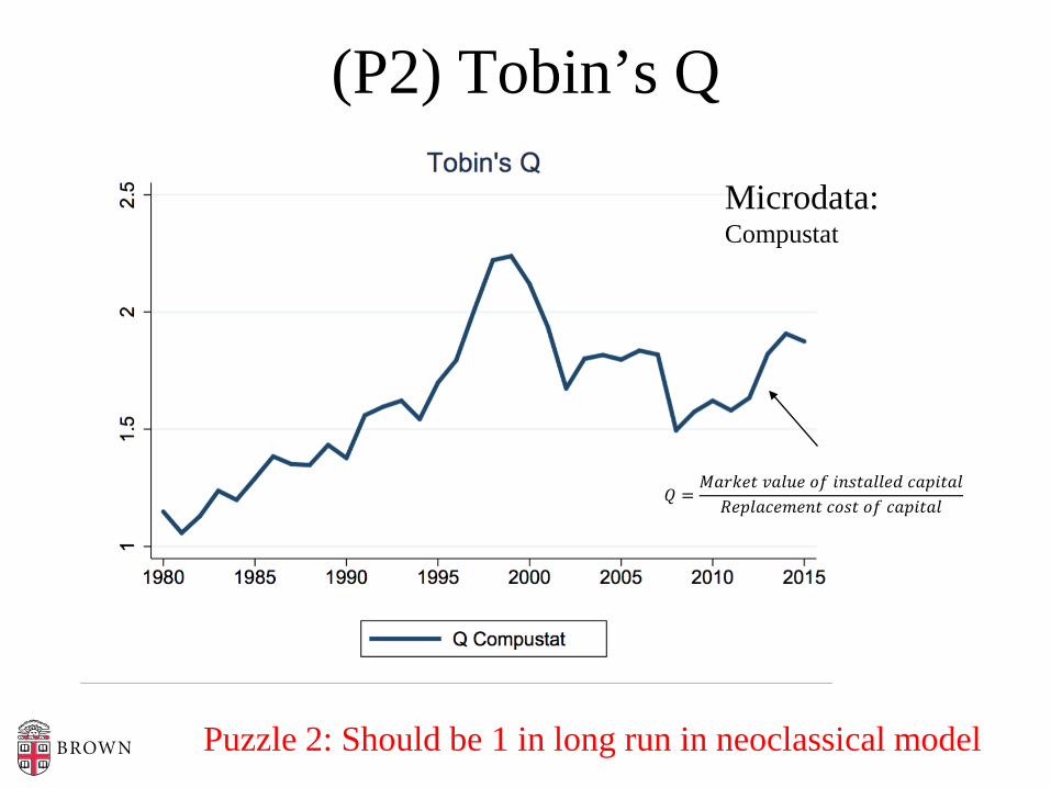
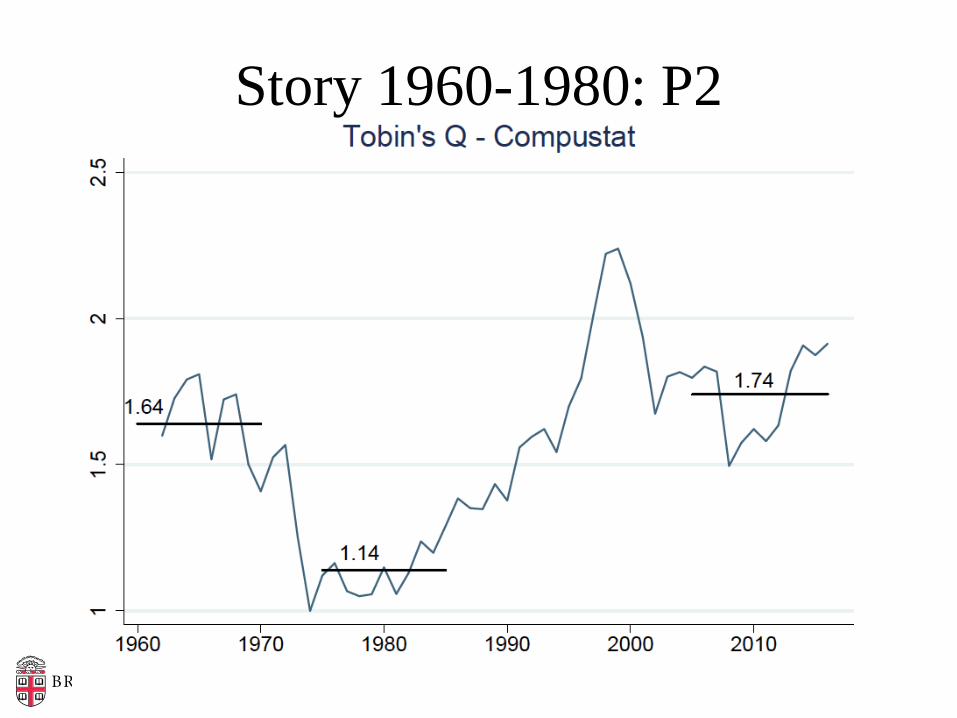
(P2) Tobin’s Q

microdata

𝑄𝑄 =𝑀𝑀𝑀𝑀𝑀𝑀𝑀𝑀𝑀𝑀𝑀𝑀 𝑣𝑣𝑀𝑀𝑣𝑣𝑣𝑣𝑀𝑀 𝑜𝑜𝑜𝑜 𝑖𝑖𝑖𝑖𝑖𝑖𝑀𝑀𝑀𝑀𝑣𝑣𝑣𝑣𝑀𝑀𝑖𝑖 𝑐𝑐𝑀𝑀𝑐𝑐𝑖𝑖𝑀𝑀𝑀𝑀𝑣𝑣𝑅𝑅𝑀𝑀𝑐𝑐𝑣𝑣𝑀𝑀𝑐𝑐𝑀𝑀𝑅𝑅𝑀𝑀𝑖𝑖𝑀𝑀 𝑐𝑐𝑜𝑜𝑖𝑖𝑀𝑀 𝑜𝑜𝑜𝑜 𝑐𝑐𝑀𝑀𝑐𝑐𝑖𝑖𝑀𝑀𝑀𝑀𝑣𝑣

Puzzle 2: Should be 1 in long run in neoclassical model

Microdata:Compustat

(P2) Tobin’s Q

“The increase in stock brings market value into line with replacement costs, lowering the former and/or raising the latter”

Tobin and Brainhard (1976)

• Standard neoclassical models predict that the value of Tobin’s Q should be 1 in long run

(P3) Decrease in real interest rate while measured return on capital constant

Gomme, Ravikumar, and Rupert (2011), NIPA

Puzzle 3: GRR and r should be same in neoclassical modelAND stable – one of Kaldor’s stylized facts

𝑅𝑅 =𝑌𝑌 − 𝑤𝑤𝑤𝑤 − 𝛿𝛿𝛿𝛿

𝛿𝛿

In neoclassical model the average return is equal to the interest rate.

(P3) Decrease in real interest rate while measured return on capital constant

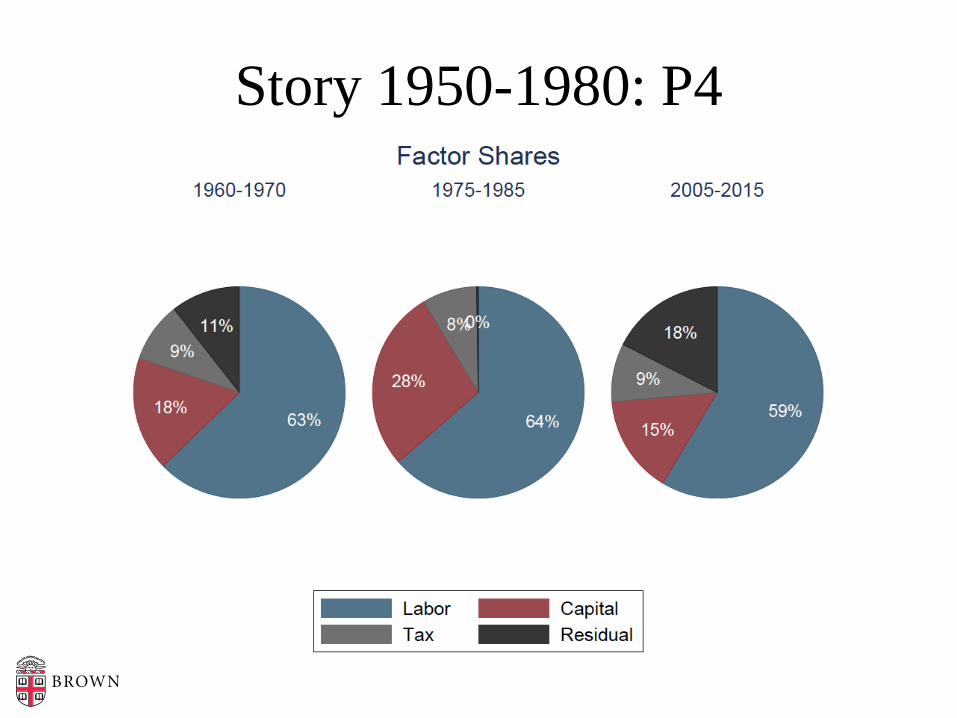
(P4) A persistent decrease in labor and capital share….

Puzzle 4: Should be constant in neoclassical model – one of Kaldor’s stylized facts

(P4) A persistent decrease in labor and capital share….

In the neoclassical model, there is no residual factor share.

(5) Decrease in investment-to-output ratio, even given low borriwng costs and high Tobin‘s Q

Puzzle 5: Should by rising given P2 and P3

Philippon and Gutierrez (2017)

(5) Decrease in investment, despite low interest rates and high Tobinds Q

Why is investment not exploding given low interest rate?

High Q?

(P1) W/Y>> despite low S and low K/Y.(P2) High Tobin’s Q >> 1.(P3) A decrease in r while measured return on capital constant.(P4) A decrease in both the labor share and the capital share.(P5) A decrease in I/Y despite low r and a high Q.

Summing up

Resolution of Puzzles

- Hypothesis: P1-P5 are being driven by two underlying trends:- An increase in monopoly power and markups- A decline in the natural rate of interest

Why them?Fall in real interest rates: Fact

Market Power• Concentration measures• Firm entry• Markup measures

• Macro• Micro

Concentration Increasing

H=∑𝑖𝑖=1𝑁𝑁 𝑖𝑖𝑖𝑖2

Common ownership correction (Compustat, Guiterrezand Phillipon (2017)

Revenue shares of largest firms increasing

US Census

Firm Entry Rates Declining

Business Dynamics Statistics, Karahan, Pugsley and Sahin (2018)

New Keynesian measures of markups

Using profit share

Barkai (2016),Neiman and Karabarboulis (2018)

Estimates from Loecker and Eechout (2017)

Compustat

Traina (2018)

Main difference:Takes into account marketing and managerial costs

Select lit reviewStanding on sholders of….

Build on large literature. About 70 references already and counting

P1: Piketty, Saez and Zucman (2018), Stiglitz (2016) …P2 : Philippon and Gutierrez (2016) …P3: Caballero, Farhi, Gourinchas (2017), Gomme, Ravikumar and Rupert (2015), Elsby, Hobijin and Sahin (2013) …P4: Barkai (2016), Caballero, Farhi, Gourinchas (2017), Karbarabounis and Neiman (2014)…P5: Phillipon and Gutierres (2016), Barkai (2016) …Markups: Autor et al (2017), De Loecker and Eechout (2017), Hall (2018), Traina (2018) ….Falling Real Rates: Del Negro et al (2017), Eggertsson, Mehrotra and Robbins (2017), Gagnon, Johannsen, Lopez-Salido (2016) ….

Outline1. Five puzzles - “stylized facts” and why neoclassical

model does not account for them. Key hypothesis for resolution

i. Increase in monopoly powerii. Secular reduction in real interest rates

2. A minimalistic modification of the canonical neoclassical model

3. Qualitative Resolution in model4. Quantitative Resolution in model

i. Estimation of driving forcesii. Calibration exercise

5. Extension

Household preferences• Unit mass of individuals with Epstein-Zin

utility:

Model – focus on production

• Final good composite

Demand of final good i Production function of final firm i

Final goods firms

• Final goods charge optimal markup

• Markups follow AR(1) process

• Barriers to entry generate pure profits

𝜇𝜇𝑡𝑡 =Λ𝑡𝑡

Λ𝑡𝑡 − 1

Firm dynamics• Although barriers, not “permanent”

• Firm exit a la Melitz (2003). Each period, a final goods firm i has a probability Δ of exiting

• Entry is also exogenous – each period, mass Δ of new final goods firms enters.

Asset pricing• There are security markets in which the rights to the

future profits of final goods firms are bought and sold

• Securities St+1 are traded at time t with price 𝑋𝑋𝑡𝑡𝑓𝑓 .

• For entering firms, shares distributed to individuals as ‘IPO Securities’

𝑋𝑋𝑡𝑡𝑓𝑓 = 𝐸𝐸𝑡𝑡�

𝑗𝑗=1

∞

(1 − ∆)𝑗𝑗−1𝑅𝑅𝑡𝑡+𝑗𝑗𝑖𝑖𝑡𝑡+𝑗𝑗𝑓𝑓

Intermediate goods firms• Representative firm

• Adjustment costs as in Jermann (1998)

Long run risk

• Long-run productivity risk enters our model as in Bansal and Yaron (2004) and Croce (2014)

• Will allow us to match equity premium

Wealth and Tobin’s Q• Define aggregate wealth as the total market value of

physical capital and securities

• Empirical Tobin’s Q is defined as

• Note that the existence of securitized pure profits allows there to be a wedge between wealth and capital, and allows Tobin’s Q to be permanently above one

𝑊𝑊𝑡𝑡 = 𝑋𝑋𝑡𝑡𝑓𝑓 + 𝑋𝑋𝑡𝑡𝑖𝑖 = 𝑋𝑋𝑡𝑡

𝑓𝑓 + 𝑞𝑞𝑡𝑡 𝛿𝛿𝑡𝑡

𝑄𝑄𝑡𝑡 =𝑊𝑊𝑡𝑡

𝛿𝛿𝑡𝑡=𝑋𝑋𝑡𝑡𝑓𝑓 + 𝑞𝑞𝑡𝑡 𝛿𝛿𝑡𝑡𝛿𝛿𝑡𝑡

Outline1. Five puzzles - “stylized facts” and why neoclassical

model does not account for them. Key hypothesis for resolution

i. Increase in monopoly powerii. Secular reduction in real interest rates

2. A minimalistic modification of the canonical neoclassical model

3. Qualitative Resolution in model4. Quantitative Resolution in model

i. Estimation of driving forcesii. Calibration exercise

Qualitative Resolution

• Consider first steady state of the model as a constant solution without uncertainty

• Can solve for P1-P5 qualitatively. • But will not be able to speak to evolution of

some financial variables like average returns that include risk premia precluding a serious quantitative evaluation.

P1

𝑊𝑊𝑌𝑌

=𝑋𝑋𝑓𝑓 + 𝑋𝑋𝑖𝑖

𝑌𝑌=𝑋𝑋𝑓𝑓

𝑌𝑌+𝛿𝛿𝑌𝑌

𝜇𝜇 − 1𝜇𝜇

1 + 𝑀𝑀 − 1 − Δ 𝑀𝑀𝜉𝜉

𝛼𝛼𝜇𝜇

𝑀𝑀 + 𝛿𝛿

𝜇𝜇 ↑ 𝑋𝑋/𝑌𝑌 ↑, 𝑀𝑀 ↓ 𝑋𝑋/𝑌𝑌 ↑ 𝜇𝜇 ↑ 𝛿𝛿/𝑌𝑌 ↓, 𝑀𝑀 ↓ 𝛿𝛿/𝑌𝑌 ↑

P2

𝑄𝑄 =𝑊𝑊𝛿𝛿

=𝑋𝑋𝑓𝑓 + 𝑋𝑋𝑖𝑖

𝛿𝛿=𝑋𝑋𝑓𝑓

𝛿𝛿∗𝛿𝛿𝑌𝑌

+ 1

(𝜇𝜇 − 1)𝛼𝛼−1(𝑀𝑀 + 𝛿𝛿)1 + 𝑀𝑀 − 1 − Δ 𝑀𝑀𝜉𝜉

𝜇𝜇 ↑ 𝑄𝑄 ↑, 𝑀𝑀 ↓ 𝑄𝑄?

P3

𝐴𝐴𝑅𝑅 =𝑌𝑌 − 𝑤𝑤𝑤𝑤 − 𝛿𝛿𝛿𝛿

𝛿𝛿=𝑀𝑀 +

𝜇𝜇 − 1𝜇𝜇

𝛿𝛿/𝑌𝑌= 𝑀𝑀 +

𝜇𝜇 − 1𝛼𝛼

(𝑀𝑀 + 𝛿𝛿)

𝜇𝜇 ↑ 𝐴𝐴𝑅𝑅 ↑, 𝑀𝑀 ↓ 𝐴𝐴𝑅𝑅 ↓

P4

𝑀𝑀 + 𝛿𝛿𝛿𝛿

=1𝜇𝜇

(1 − 𝛼𝛼)

𝑤𝑤𝑤𝑤𝑤𝑤

=1𝜇𝜇𝛼𝛼

𝜇𝜇 ↑𝑀𝑀 + 𝛿𝛿𝛿𝛿

↓𝑤𝑤𝑤𝑤𝑤𝑤↓

P5

𝐼𝐼𝑌𝑌

=𝛼𝛼(𝛿𝛿 + 𝜖𝜖𝜁𝜁 − 1)𝜇𝜇(𝑀𝑀 + 𝛿𝛿)

𝛼𝛼𝜇𝜇 ↑

𝐼𝐼𝑌𝑌↓, 𝑀𝑀 ↓

𝐼𝐼𝑌𝑌↓

Can we match puzzles?-- simple model

2.6 (2.54) 0.7 (0.71) 0.18 (0.17) 0.07 (0.12) 1.18 (1.14)

r=3% r=1% 𝜇𝜇=1.1 𝜇𝜇=1.22

3.39 (3.63) 0.63 (0.64) 0.17 (0.16) 0.08 (0.13) 1.32 (1.74)

𝛿𝛿 = 0.06 𝛼𝛼 = 0.23 𝜟𝜟 = 𝟎𝟎.𝟐𝟐𝟐𝟐 Δ, 𝛿𝛿, 𝛼𝛼, 𝜇𝜇, r, 𝑀𝑀𝜉𝜉

Outline1. Five puzzles - “stylized facts” and why neoclassical

model does not account for them. Key hypothesis for resolution

i. Increase in monopoly powerii. Secular reduction in real interest rates

2. A minimalistic modification of the canonical neoclassical model

3. Qualitative Resolution in model4. Quantitative Resolution in model

i. Estimation of driving forcesii. Calibration exercise

5. Extensions

Quantitative Analysis

• We’ve seen how an increase in monopoly power combined with a decrease in r can potentially account for the five facts

• But are these effects quantitatively important?

Quantitative experiment• Do a second order approximation of the model.• Calibrate the model to 1970. • Then “plug in” Change in markups from 1970 level to 2015 level Changes in interest rates from 1970 to 2015 level

• Compare changes in model moments to changes in data moments, see if we can match the puzzles

Quantitative Exercise

3 categories categories of parameters and shocks1. Levels of markups and interest rates2. Parameters from data and literature3. Parameters chosen to match 1970 data moments, through minimization of objective function

(1) Markups

Our estimate: Using methods similar to Barkai, find increase from 1.11 to 1.22 from 1970-2015

(1) Changes in the natural rate

Our estimate: Decline of 2%, from 3% in 1970 to 1% in 2015

(2) Parameters taken from the literature

(3) Parameters calibrated to 1970 moments

(3) Parameters calibrated to 1970 moments

Calibration• Note that we are choosing parameters to

match only 1970 moments• In particular, we do not choose any

parameters to match 2015 moments, or to try and match any change in the moments from 1970 to 2015

• The success or failure of the exercise will be comparing changes in our model moments to change in the data moments

Results – Markups & Interest Rates

Results

• Overall the markups and drop in real interest rate can “quantitatively account” for P1-P5

Results – markup only

Results – interest rate only

Other estimate of markups

• Using Nakarda-Ramey yields very similar results

• De Loecker and Eeckout (2017)

Other stories, extensions• Housing to be added• Fall in relative price of investment to be added.• Implausible implications for other shocks?• Other candidates

– Rise in risk-premia– in our case it is endogenous– Intangible capital

• What about pre-1970?• Endogenous rise in markups

Intangible capital story

• Another story --- there is a still a large stock of unmeasured intangible capital

• This would lead to a high measured Q, average return, and W/Y…..

However…• Last two revisions to NIPAs have included

massive revisions of intangible capital

• Most expenditures on R&D, software, training, etc are now counted as investment

• What potential intangible investment is missing? Advertising, marketing (Traina2018), etc. – But is this investment? ”creates” market power

Story 1960-1980: P1

The picture can't be displayed.The picture can't be displayed.

Story 1960-1980: P2

Story 1960-1980: P3

Story 1950-1980: P4

Story 1960-1980: P5

Story 1950-1980: Markups

Can we match puzzles?-- simple model

2.6 (2.54) 0.7 (0.71) 0.18 (0.17) 0.07 (0.12) 1.18 (1.14)

r=3% r=2% 𝜇𝜇=1.1 𝜇𝜇=1.15

3 (2.8) 0.66 (0.63) 0.19(0.16) 0.08 (0.15) 1.28(1.64)

𝛿𝛿 = 0.06 𝛼𝛼 = 0.23 𝜟𝜟 = 𝟎𝟎.𝟐𝟐𝟐𝟐 Δ, 𝛿𝛿, 𝛼𝛼, 𝜇𝜇, r, 𝑀𝑀𝜉𝜉

Pre 1980 Story

• Overall story consistent with a moderate level of markups in 1960, followed by a decline until 1980, followed by a significant increase

Firm Entry Rates Declining: Endogenous markups

• Countinum of industries on measure 0 to 1.

• Finite number of firms in industry

• Berntrand competition.

Atkeson-Burstein (2008)Jaimovich and Floetotto (2008)

Simples case: Elasticity across industries 1, then

N down by 20%𝜇𝜇 from 1.4 to 1.5

ConclusionP1-P5 circumstantial evidence for higher markups To early to draw policy conclusions

– Needed: Explicit model where the monopoly “wedge” is explicitly modeled.

Highermarkups Benevolent

(R&D gives rise to temporary advantages that are efficient

Malignant development(less antitrust!)

Conclusion• Analysis relies heavily on estimates of

markups, which are difficult to measure. Having said that, an increase in markups should lead to…– Negative impact on GDP growth– Increase in income inequality and wealth

inequality– Important implications for capital taxation?

Back to fact 1

Definition: A pure capital gain is the aggregate increase in the market value of household wealth beyond what is saved.

Gross national capital gain

Gross National Capital Gains

Gross National Capital Gains

Distribution of capital gains

Effect on top income shares

Effect on top income shares

(P2) Macro Tobin’s Q

Bob Hall (2001)

Philippon and Gutierrez (2017)

Macrodata:Flow of Funds by Fed

𝑄𝑄 =𝑀𝑀𝑀𝑀𝑀𝑀𝑀𝑀𝑀𝑀𝑀𝑀 𝑣𝑣𝑀𝑀𝑣𝑣𝑣𝑣𝑀𝑀 𝑜𝑜𝑜𝑜 𝑖𝑖𝑖𝑖𝑖𝑖𝑀𝑀𝑀𝑀𝑣𝑣𝑣𝑣𝑀𝑀𝑖𝑖 𝑐𝑐𝑀𝑀𝑐𝑐𝑖𝑖𝑀𝑀𝑀𝑀𝑣𝑣𝑅𝑅𝑀𝑀𝑐𝑐𝑣𝑣𝑀𝑀𝑐𝑐𝑀𝑀𝑅𝑅𝑀𝑀𝑖𝑖𝑀𝑀 𝑐𝑐𝑜𝑜𝑖𝑖𝑀𝑀 𝑜𝑜𝑜𝑜 𝑐𝑐𝑀𝑀𝑐𝑐𝑖𝑖𝑀𝑀𝑀𝑀𝑣𝑣

Change in Revenue Share