Embed Size (px)
Citation preview

WP/16/160
Testing Piketty’s Hypothesis on the Drivers of Income Inequality: Evidence from Panel VARs with Heterogeneous Dynamics
by Carlos Góes
IMF Working Papers describe research in progress by the author(s) and are published
to elicit comments and to encourage debate. The views expressed in IMF Working Papers
are those of the author(s) and do not necessarily represent the views of the IMF, its
Executive Board, or IMF management.
© 2016 International Monetary Fund WP/16/160
IMF Working Paper
Western Hemisphere Department
Testing Piketty’s Hypothesis on the Drivers of Income Inequality: Evidence from Panel
VARs with Heterogeneous Dynamics
Prepared by Carlos Góes1
Authorized for distribution by Alfredo Cuevas
August 2016
Abstract
Thomas Piketty's Capital in the Twenty-First Century puts forth a logically consistent
explanation for changes in income and wealth inequality patterns. However, while rich in
data, the book provides no formal empirical testing for its theoretical causal chain. In this
paper, I build a set of Panel SVAR models to check if inequality and capital share in the
national income move up as the r-g gap grows. Using a sample of 19 advanced economies
spanning over 30 years, I find no empirical evidence that dynamics move in the way Piketty
suggests. Results are robust to several alternative estimates of r-g.
JEL Classification Numbers: O43, C33, C14, C12
Keywords: Income Inequality, Panel VAR, Factor Income Distribution
Author’s E-Mail Address: [email protected]
1 International Monetary Fund (WHD). I wholeheartedly thank Branko Milanovic, Peter Pedroni, Roberto
Perrelli, Henrique Barbosa, Franz Loyola, Cornelius Fleischhaker, Marcelo Estevão, Troy Matheson, Iza
Karpowicz, Michele Andreolli, Alexandra Martinez, Alfredo Cuevas, and participants of the WHDS1 seminar
for their helpful comments. All errors and omissions are solely mine. This paper is fully reproducible: data and
econometric programs are available at https://github.com/omercadopopular/cgoes.
IMF Working Papers describe research in progress by the author(s) and are published to
elicit comments and to encourage debate. The views expressed in IMF Working Papers are
those of the author(s) and do not necessarily represent the views of the IMF, its Executive Board,
or IMF management.

Contents
Page
1 Introduction . . . . . . . . . . . . . . . . . . . . . . . . . . . . . . . . . . . . . . . . . . 4
2 Piketty’s Model: What to Test . . . . . . . . . . . . . . . . . . . . . . . . . . . . . . . 4
3 Data and Stylized Facts . . . . . . . . . . . . . . . . . . . . . . . . . . . . . . . . . . . 6
4 Methodology . . . . . . . . . . . . . . . . . . . . . . . . . . . . . . . . . . . . . . . . . . 8
5 Empirical Models and Results . . . . . . . . . . . . . . . . . . . . . . . . . . . . . . . 9
6 Robustness . . . . . . . . . . . . . . . . . . . . . . . . . . . . . . . . . . . . . . . . . . . 21
7 Discussion: What is the Takeaway? . . . . . . . . . . . . . . . . . . . . . . . . . . . . 22
8 Conclusions . . . . . . . . . . . . . . . . . . . . . . . . . . . . . . . . . . . . . . . . . . . 24
A Appendix: Data and Sources . . . . . . . . . . . . . . . . . . . . . . . . . . . . . . . . 26A.1 Countries Sample . . . . . . . . . . . . . . . . . . . . . . . . . . . . . . . . . . . . . . 26A.2 Data Sources . . . . . . . . . . . . . . . . . . . . . . . . . . . . . . . . . . . . . . . . 26
B Appendix: Standard Error Simulation Algorithm . . . . . . . . . . . . . . . . . . . 27
List of Figures
1 Distribution of capital share and share of the top 1% over time . . . . . . . . . . . . 72 Contemporaneous correlations between r− g spread and capital share or share of the
top 1% . . . . . . . . . . . . . . . . . . . . . . . . . . . . . . . . . . . . . . . . . . . . 73 Results of Model 1: Heterogeneous composite impulse responses across sample . . . 104 Results of Model 1: Median composite responses and confidence intervals . . . . . . 115 Results of Model 1: Decomposition of median composite responses . . . . . . . . . . 126 Correlation between heterogeneous responses and intergenerational elasticity of in-
come and social expenditure, respectively . . . . . . . . . . . . . . . . . . . . . . . . 137 Results of Model 2: Heterogeneous composite impulse responses across sample . . . 148 Results of Model 2: Median composite responses and confidence intervals . . . . . . 159 Results of Model 2: Decomposition of median composite responses . . . . . . . . . . 1610 Contemporaneous correlation between GDP growth and changes in the savings rate 1711 Results of Model 3: Heterogeneous composite impulse responses across sample . . . 1812 Results of Model 3: Median composite responses and confidence intervals . . . . . . 1913 Results of Model 3: Decomposition of median composite responses . . . . . . . . . . 2014 Robustness checks . . . . . . . . . . . . . . . . . . . . . . . . . . . . . . . . . . . . . 21
3
1 Introduction
Capital in the Twenty-First Century, Thomas Piketty’s magnum opus, has been widely praised foraggregating and presenting in a timely and accessible fashion the results of more than a decade ofresearch spearheaded by Piketty and his co-authors. His work is likely to remain influential in thetimes to come, not only for its databases, which map the (traditionally scarce) information aboutincome inequality but also because it is inspiring many economists to use the estimation techniqueshe and his co-authors popularized.
Piketty’s theoretical explanations for changes in inequality patterns are interesting. In a nutshell,he argues that all other things constant, whenever the difference between the returns on capital(r) and the output growth rate (g) increases, the share of capital in national income increases.Furthermore, since capital income tends to be more unequally distributed than labor income, anincrease of the capital share would likely lead to increased overall income (and, over time, wealth)inequality. Both of these are plausible relationships. However, while rich in data, Capital providesno formal empirical testing for these conjectures. In fact, there is little more than some apparentcorrelations the reader can eyeball in charts containing very aggregated multi-decennial averages.
The main contribution of this paper is to provide a rigorous empirical test of Piketty’s hypotheses.For that purpose, I build Panel Structural Vector Autoregressive models to test if inequality and thecapital share in the national income increase as the r − g gap grows. I use Pedroni’s (2013) recentPanel VAR technique, which controls for country fixed-effects and allows for full heterogeneity ofdynamics across countries, to estimate these relationships in a panel of 19 advanced economiesspanning over 30 years. This technique results in a distribution of impulse response functions,permitting a much more robust inference than those that rely on average estimates and assumeslopes are homogeneous.
I find no empirical evidence that the dynamics move in the way Piketty suggests. In fact, for atleast 75% of the countries examined, inequality responds negatively to r− g shocks, which is in linewith previous single-equation estimates by Acemoglu and Robinson (2015). The results also suggestthat changes in the savings rate, which Piketty takes as relatively stable over time, are likely to offsetmost of the impact of r − g shocks on the capital share of the national income. Thus, it providesempirical evidence to the model developed by Krusell and A. Smith (2015), who say Piketty relieson flawed theory of savings. The conclusions are robust to alternative estimates of r − g and to theexclusion or inclusion of tax rates in the calculation of the real return on capital.
Knowing if Piketty’s hypothesis is correct is of crucial importance. Such is the case because thepolicy solutions designed to counter increasing income inequality trends in advanced economies willneed to tackle the underlying causes of inequality. The results presented here show that observedincreases in income inequality in advanced economies are largely uncorrelated with changes in r− g,which suggests that one needs to look for the causes of inequality (and potential solutions) elsewhere.
This paper outlines Piketty’s theoretical model and develops a strategy to test it. First, I presenta simplified description of the basic theoretical relationships Piketty proposes. Then I describethe data and how I constructed some of the variables of interest and explain the methodology ofthe structural Panel VAR. I then present the results (paying special attention to how to interpretheterogeneous dynamics), perform some robustness tests, and try to relate the set of results to thebulk of the literature on income inequality, pointing to potential causes of increasing inequalitywhich are not related to r− g. Finally, I conclude by summarizing the most important points of thepaper and what they mean for future inequality dynamics.
2 Piketty’s Model: What to Test
Building on a standard growth model, Piketty (2014) argues that the patterns of wealth and incomeconcentration are defined by the difference in the real return on capital (r) and growth rates (g).
4
Here, I present a very stylized derivation of Piketty’s model and its implications, so as to develop atesting strategy.
In a closed economy where national income (Y ) is a function of capital (K) and labor (L),Yt = Kα
t L1−αt , defining the real return on capital as the marginal product of capital (r ≡ ∂Yt
∂Kt),
means that the share of capital in the national income (α) can be represented as a function of thereal rate of return on capital (r), since r = ∂Yt
∂Kt= α Yt
Kt. This basic definition is what Piketty calls
the “first fundamental law of capitalism”:
α =rKt
Yt(1)
If the law of motion of capital is Kt+1 = (1 − δ)Kt + sYt, where s is a constant savings rate, δis a constant rate of depreciation, the population is constant, and Yt+1 = (1 + g)Yt, at the steady
state ddt
[Kt
Yt
]= 0, which implies:
K
K=
Y
Y,
sY − δKK
=gY
Y,
K
Y=
s
g + δ(2)
where bars denote variables at their steady states. Piketty defines all of his variables in netterms, such that one should deduct depreciation from income, capital, and the savings rate. But,since both expressions are equivalent in their steady states (cf. Krusell and A. Smith 2015), andmost standard textbooks use variables in gross terms, it is more expedient to explicitly to accountfor depreciation.
Substituting (2) into (1) yields what Piketty calls the “second fundamental law of capitalism”—an inverse relationship between the share of capital in the national income and economic growth:
α =rs
g + δ(3)
Dynamically, once one introduces random shocks to the steady state, one can think of the capitalshare (α) an moving average process centered around a steady state:
αt = α+ Φ(L)ξt (4)
where Φ(L) ≡ (∑∞j=0 ΦjL
j) is a polynomial of responses to stochastic innovations and ξt is anexogenous shock.
Taking the (net) savings rate as somewhat constant, Piketty and Zucman (2015) argue that thecapital share, income inequality, and wealth inequality are rising functions of r − g. If Piketty iscorrect, then one should expect changes in the share of capital to be explained by contemporaneousand past changes in the spread between r and g (or, using the textbook model, between r andg + δ). This means that all other things equal, a temporary exogenous innovation to r − g shouldbe expected to disturb the steady state and temporarily take α away from it in the same directionof the innovation. That is, if growth temporarily increases (or real return on capital decreases), thecapital share is expected to temporarily fall. Piketty goes on to argue that as the returns on capitalare more unequally distributed than labor income, a higher share of capital in the national incomewould lead to higher income and wealth inequality (Piketty 2014, ch. 7).
These relationships are empirical propositions and hence empirically testable. The testable hy-pothesis is that positive changes in r− g lead to positive changes in inequality (z) and capital share(α). If there is no robust evidence for the baseline hypothesis (Hb), one cannot reject the alternativehypothesis (Ha) of zero (or negative) association between these variables:
5

Hb : if ∆(r − g) > 0, then ∆z > 0, ∆α > 0
Ha : if ∆(r − g) > 0, then ∆z ≤ 0, ∆α ≤ 0
Piketty stresses that these dynamics are long-run and asymptotic, hinting at potential difficultiesin capturing them. Still, if his assumptions are correct, in a large enough sample, the observeddynamics should at least provide some evidence of such underlying relationships.
3 Data and Stylized Facts
In order to analyze the relationship between inequality, capital share and returns on capital to GDPgrowth differentials, I organize data from multiple sources. Data availability varies by country andthe maximum range goes from 1980 through 2012. Data on the capital share and share of the top 1%are more reliable for advanced economies. For such reason, the final sample is an unbalanced longpanel with annual observations for 19 advanced economies from different continents (see AppendixA for details).
Inequality is proxied by the share of national income held by the top 1%, as reported by Atkison’s& Piketty’s World Top Incomes Database. The choice of such variable is rather obvious since thisis Piketty’s measure of choice (as compared to alternative metrics, like the Gini index) to indicaterising inequality in advanced economies in the past decades. The annual capital share in the nationalincome comes from the Penn World Tables.
To derive the second variable of interest —namely, the real return on capital net of real GDPgrowth —I take yearly averages of nominal long-term sovereign bond yields, calculate the post-taxnominal rates by deducting corporate income taxes and subtract from them annual percent changesin GDP deflators and real GDP growth. The r in r − g is, then:
ri,t = [(1− τi,t)ii,t − di,t] (5)
where ri,t is the real return on capital, τi,t is the corporate income tax rate, ii,t is the nominallong-term sovereign bond yield, and di,t is the annual percent change in the GDP deflator for countryi at period t. GDP deflators and real growth rates are found in the IMF’s World Economic Outlookdatabase. Tax rates come mostly from the OECD’s Tax Database —with the exception of the timeseries for Singapore, which was constructed independently.
The choice of sovereign bond yields as a proxy for returns on capital is not self-evident. In reality,the aggregate return on capital is a weighted average of returns across a plethora of investments.However, returns on government bonds are a good proxy for the purposes of this empirical exercise fortwo reasons. First, Piketty’s narrative centers on worries about a society facing the unmeritocraticrule of rentiers who profit from high returns on capital, which he illustrates by discussing how 19th
century elites profited from high returns on government bonds (Piketty 2014, p. 132). Second, evenif the level of return is different for different portfolios, the correlation between sovereign bondsand corporate bonds is historically very high. In fact, between 1996 and 2015, the correlationbetween prime AAA corporate bonds and U.S. treasuries was nearly perfect (r = 0.93); even whenconsidering “junk” BB+ graded corporate bonds the co-movement between sovereigns and corporateswas relatively tight (r = 0.49).
In the robustness section, I present results with two different proxies for r: short-term interestrates, and implied returns from the national accounts. I also present results ignoring tax rates.
Distributions of capital share and share of the top 1% in the sample show increasing trends,although with some signs of moderation in the late 2000s due to the global financial crisis. Theupward trend is observed not only in the medians but also in the evolution of interquartile ranges,as shown in Figure 1.
6

0
10
20
30
40
50
60
1980-89 1990-99 2000-05 2005-100
2
4
6
8
10
12
14
16
18
20
1980-89 1990-99 2000-05 2005-10
Share of the Top 1%Capital Sharein p
erce
nt o
f nat
iona
l inc
ome
in p
erce
nt o
f nat
iona
l inc
ome
Figure 1: Distribution of capital share and share of the top 1% over time. Y-axis inpercent, x-axis represents period averages. The sample refers to an unbalanced panel of 19 advancedeconomies ranging from 1981-2010. Boxplots show interquartile ranges and medians. Whiskers showminimums and maximums.
Basic stylized facts can provide some preliminary insights regarding whether or not the data sup-port Piketty’s assertions. Figure 2 plots the contemporaneous correlations between r−g spreads andcapital share, and share of the top 1%. Such basic correlations show no evidence of the relationshipPiketty poses. Rather, the variables seem largely orthogonal.
y = 0.0257x + 0.0603R² = 0.004, n = 532
-10
-5
0
5
10
-15 -10 -5 0 5 10 15
Demeaned (r - g)
Dem
eane
d sh
are
of T
op 1
%
y = -0.0709x + 0.1046R² = 0.0078, n = 532
-10
-5
0
5
10
-15 -10 -5 0 5 10 15
Demeaned (r - g)
Dem
eane
d ca
pita
l sha
re
Figure 2: Contemporaneous correlations between r− g spread and capital share or shareof the top 1%, respectively. The sample refers to an unbalanced panel of 19 advanced economiesranging from 1981-2012. Variables are demeaned to account for time-invariant country-specificcharacteristics.
If the absence of a positive relationship persists with more refined estimation techniques, thiscould raise questions about Piketty’s assertion that a higher r− g will lead to higher inequality overthe coming century. In the next section, I describe a model to test precisely that.
7

4 Methodology
Following Pedroni (2013), I estimate a structural Panel VAR that accommodates country-fixedeffects, allows dynamics to be fully heterogeneous amongst panel members and decomposes dynamicsbetween different responses to idiosyncratic and common shocks. In that context, for each memberi = [1, ...,M ]′ of an unbalanced panel, let yi,t be a vector of n endogenous variables with country-specific time dimensions t = [1, ..., Ti]
′. To control for individual fixed-effects, I demean the data,
resulting in y∗i,t = yi,t − yi, where yi ≡ T−1i
∑Ti
t=1 yi,t∀i. The baseline model is:
Biy∗i,t = Ai(L)y∗i,t−1 + ei,t (6)
where y∗i,t is a n-dimensional vector of demeaned stacked endogenous variables, Ai(L) is a poly-
nomial of lagged coefficients [Ai(L) ≡ (∑Jij=0A
ijL
j)] with country-specific lag-lengths Ji, Aij is a
matrix of coefficients, ei,t is a vector of stacked residuals, and Bi is a matrix of contemporaneouscoefficients. Ji are selected based on appropriate criteria to assure that residuals approximate whitenoise.
To allow for heterogeneous dynamics, I first estimate and identify reduced-form VARs for eachcountry i:
B1y∗1,t = A1(L)y∗1,t−1 + e1,t
... (7)
BMy∗M,t = AM (L)y∗M,t−1 + eM,t
and then estimate another auxiliary VAR to recover common dynamics. Common dynamics arecaptured by averages, across individuals, for each period (y∗t ≡M−1
∑Mi=1 y
∗i,t):
By∗t = A(L)y∗t−1 + et (8)
After transforming the reduced-form residuals in (2) and (3) into their structural equivalents(ui,t = B−1i ei,t and ut = B−1et, respectively), I run nM OLS regressions to decompose the shocksinto two terms:
u1,t = Λ1ut + u1,t... (9)
uM,t = ΛM ut + uM,t
where ui,t are composite shocks, ui,t are common shocks, ui,t are idiosyncratic shocks, and Λi aren-by-n diagonal matrices with country specific loadings (the coefficients from the OLS regressions)denoting the relative importance of common shocks for each country. Note that ui,t vectors aretruly idiosyncratic, since they are by construction orthogonal to the shocks derived from the averagedynamics shared by all panel members.
Subsequently, I use standard methods described in Lutkepohl (2007) to recover the matrices ofcomposite responses to structural shocks [Ri(L)] for each country, which are shown below in thevector moving average representations of M structural VARs:
y∗1,t = R1(L)u1,t
... (10)
y∗M,t = RM (L)uM,t
8

and then use the loading matrices estimated in (9) to decompose the composite responses intocountry-specific responses to common shocks and responses to idiosyncratic shocks:
R1(L) = Λ1R1(L) + (I − Λ1Λ′1)R1(L)
... (11)
RM (L) = ΛMRM (L) + (I − ΛMΛ′M )RM (L)
Equivalently, Ri(L) = Ri(L) + Ri(L), where Ri(L) ≡ ΛiRi(L) and Ri(L) ≡ (I − ΛiΛ′i)Ri(L). I
then use the cross-sectional distribution of Ri(L), Ri(L) and Ri(L) to describe some properties of thecollection of impulse response functions calculated, such as their medians, averages and interquartileranges.
After recovering the point estimates of all the impulse response functions, I calculate standarderrors of medians through a re-sampling simulation repeating all the steps above 500 times (seeAppendix B for details).
5 Empirical Models and Results
I run three models with the methodology described above:
• In Model 1, yi,t ≡ [pi,t, zi,t]′, where zi,t is the national income share of the top 1% for country
i at period t and pi,t ≡ (ri,t−gi,t) is the post-tax return on capital (r) net of real GDP growth(g).
• In Model 2, yi,t ≡ [pi,t, ki,t]′, where ki,t is the share of capital in national income.
• In Model 3, yi,t ≡ [pi,t, si,t, ki,t]′, incorporating the savings rate (si,t).
Note that, since the data are demeaned to control for country-fixed effects, if one takes the rateof depreciation as time-invariant, even if different for each country, it is not necessary to explicitlyaccount for it in the empirical model. Depreciation is treated away once the data are demeaned asp∗i,t ≡ (ri,t − gi,t)∗ = (ri,t − gi,t − δi)∗.
The identification strategies of the empirical model the theoretical model proposed by Piketty:i.e., I take r−g as the (most) exogenous variable. This means that I impose short-run lower triangularrestrictions in the contemporaneous coefficients such that r−g contemporaneously impacts the shareof the top 1% and the capital share and r− g responds to shocks to the share of the top 1% and thecapital share only with a lag. In the robustness section, I present results with the inverse restrictions.
Pedroni’s methodology allows for fully heterogeneous dynamics. This means that the results ofthe Panel VAR are more than average parameters and average impulse response functions —as theyare in traditional panels, which impose homogeneous parameters. Rather, I have information aboutseveral moments of the distributions of impulse responses for each response horizon. With thosedata, I can then plot averages, medians and interquartile ranges of responses for a given horizon, asshown in Figure 3.
This is a much more informative way of reading results than in traditional panel VAR analyses.For instance, had I calculated average impulse responses from parameters estimated with traditionaldynamic panels (e.g., difference or system GMM equations), I would have no way of knowing howmany countries in the sample have dynamics that are similar to the average dynamics —as theunderlying assumption is that parameters are equal for all countries. Effectively, knowing exactlyhow many countries in the sample present certain dynamics provides for much more robust inferencethan simply relying on average estimates. In addition to that, as shown by Pesaran & Smith (1995),
9

if individual dynamics are heterogeneous, aggregating or pooling slopes can lead to biased estimates,making individual regressions for each group member preferable.
Despite country-specific heterogeneity, the estimated VARs are stable and the variables are(trend) stationary. This means shocks should be interpreted as temporary and, following any shock,variables are expected to converge back to their means or deterministic trends over the long run.Assuming shocks are permanent would not affect the qualitative interpretation of results since thiswould simply mean accumulating temporary responses.
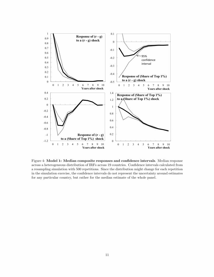
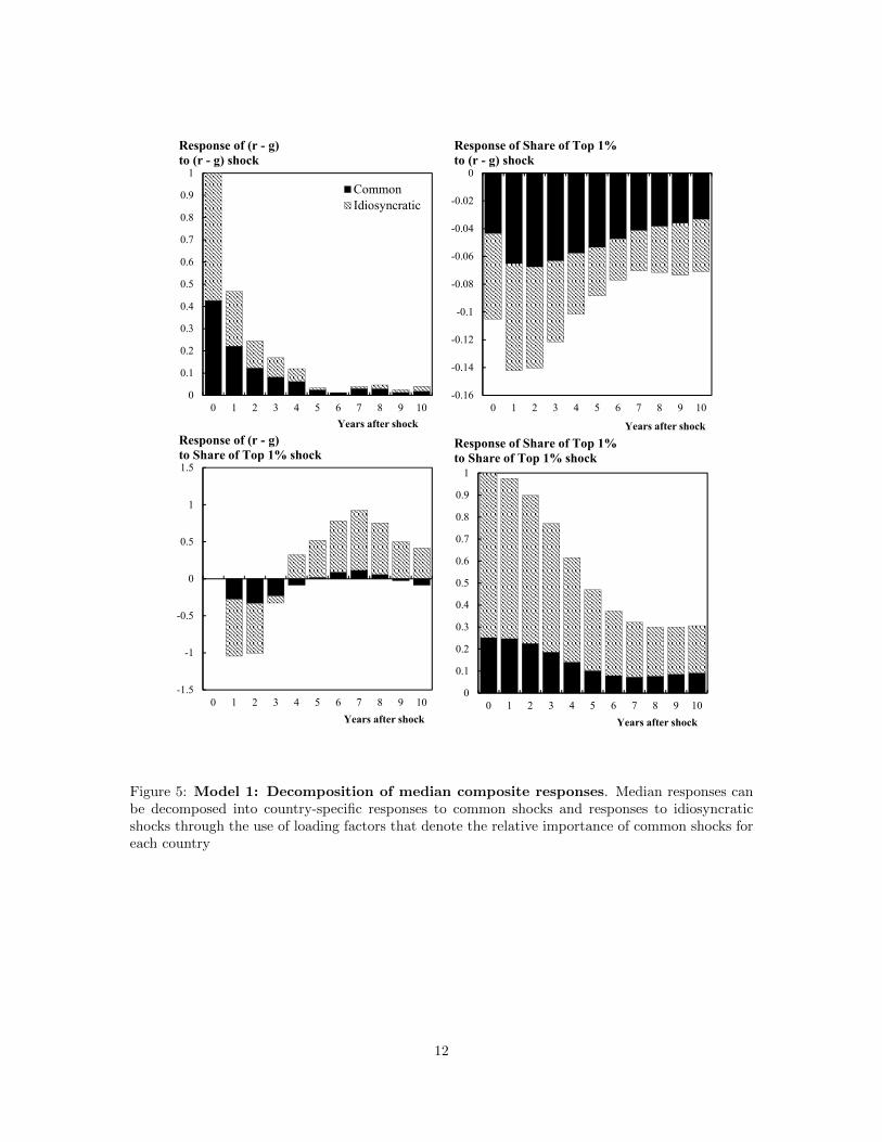
The results of Model 1 show that for at least 75% of the countries an exogenous 1% positiveshock to r − g leads to an expected decrease in the share of the top 1% in the first five years (seeFigure 3). While the median response is not statistically significant contemporaneously, it is negativeand statistically significant from the first through the tenth year after the initial shock (see Figure4). The responses to common and idiosyncratic shocks have the same (negative) sign. This is achallenge to the narrative which argues that systemic forces (as, for instance, globalization) couldbe exacerbating inequality as returns on capital increase (see Figure 5).Figure #. Country Name: Title, Date
Source:
0
0.1
0.2
0.3
0.4
0.5
0.6
0.7
0.8
0.9
1
1.1
0 1 2 3 4 5 6 7 8 9 10
Interquartile rangeMedianAverage
Response of (r - g)to a (r - g) shock
Years after shock
-0.4
-0.35
-0.3
-0.25
-0.2
-0.15
-0.1
-0.05
0
0.05
0.1
0 1 2 3 4 5 6 7 8 9 10Years after shock
Response of (Share of Top 1%)to a (r - g) shock
-2.5
-2
-1.5
-1
-0.5
0
0.5
1
1.5
2
2.5
0 1 2 3 4 5 6 7 8 9 10
Years after shock
Response of (r - g)to a (Share of Top 1%) shock
0
0.2
0.4
0.6
0.8
1
1.2
1.4
0 1 2 3 4 5 6 7 8 9 10
Years after shock
Response of (Share of Top 1%) to a (Share of Top 1%) shock
Figure 3: Model 1: Heterogeneous composite impulse responses across sample. Themedian, averages, and interquartile ranges were calculated from the distribution of IRFs of the 19cross-sections.
10
0
0.1
0.2
0.3
0.4
0.5
0.6
0.7
0.8
0.9
1
0 1 2 3 4 5 6 7 8 9 10
Response of (r - g)to a (r - g) shock
-0.5
-0.4
-0.3
-0.2
-0.1
0
0.1
0 1 2 3 4 5 6 7 8 9 10
95%confidenceinterval
Response of (Share of Top 1%)to a (r - g) shock
-1
-0.8
-0.6
-0.4
-0.2
0
0.2
0.4
Response of (r - g) 0.2
0.4
0.6
0.8
1
1.2
1.4 Response of (Share of Top 1%) to a (Share of Top 1%) shock
Years after shock Years after shock
-1.2
-1
-0.8
0 1 2 3 4 5 6 7 8 9 10
Response of (r - g)to a (Share of Top 1%) shock
0
0.2
0 1 2 3 4 5 6 7 8 9 10Years after shock Years after shock
Figure 4: Model 1: Median composite responses and confidence intervals. Median responseacross a heterogeneous distribution of IRFs across 19 countries. Confidence intervals calculated froma resampling simulation with 500 repetitions. Since the distribution might change for each repetitionin the simulation exercise, the confidence intervals do not represent the uncertainty around estimatesfor any particular country, but rather for the median estimate of the whole panel.
11
-0.16
-0.14
-0.12
-0.1
-0.08
-0.06
-0.04
-0.02
0
0 1 2 3 4 5 6 7 8 9 10
Response of Share of Top 1%to (r - g) shock
Years after shock
0
0.1
0.2
0.3
0.4
0.5
0.6
0.7
0.8
0.9
1
0 1 2 3 4 5 6 7 8 9 10
Response of Share of Top 1%to Share of Top 1% shock
Years after shock
0
0.1
0.2
0.3
0.4
0.5
0.6
0.7
0.8
0.9
1
0 1 2 3 4 5 6 7 8 9 10
CommonIdiosyncratic
Response of (r - g)to (r - g) shock
Years after shock
-1.5
-1
-0.5
0
0.5
1
1.5
0 1 2 3 4 5 6 7 8 9 10
Response of (r - g)to Share of Top 1% shock
Years after shock
Figure 5: Model 1: Decomposition of median composite responses. Median responses canbe decomposed into country-specific responses to common shocks and responses to idiosyncraticshocks through the use of loading factors that denote the relative importance of common shocks foreach country
12

One of the advantages of estimating heterogeneous slopes is that one can explore the variabilityin parameters across the cross-sectional dimension of the panel. One can do that by correlatingthe response magnitudes of the different countries in the sample with potential covariates. I plotbelow some bivariate relationships which can provide some intuition on the causes and effects of theexistent heterogeneity in responses.
There is a positive correlation between estimates of the intergenerational elasticity of income—which measures the share of a person’s income is explained by the parent’s income —and the sizeof the contemporaneous response of inequality to r− g shocks. This hints on the idea that a highertransmission between r− g and the share of the top 1% leads to a higher observed level of wage andwealth persistence.
Similarly, contemporaneous responses of inequality to r− g shocks are positively correlated withsocial expenditure as a share of GDP for countries in the sample. This suggests that societies whichare more vulnerable to larger shocks to inequality tend to be more willing to resort to governmentin order to provide social services. This would be a Rawlsean interpretation on how to hedge one’sexposure to inequality under a “veil of ignorance” about the future: insofar as social services areusually targeted at the lower end of income distribution, they can be seen as a kind of insuranceagainst higher market income inequality.
Such correlations are shown as simple bivariate scatterplots in Figure 6.
AUS
CANFIN
FRA
DEUIRL
ITA
JPN
NET
NZL
NOR
PRT
ESP
SWE
CHEGBR
USA
y = 0.2892x + 0.4014R² = 0.1413
p < 0.17
0
0.1
0.2
0.3
0.4
0.5
0.6
0.7
0.8
-0.8 -0.6 -0.4 -0.2 0 0.2 0.4
Inte
rgen
erat
iona
l Ela
stic
ityof
Inco
me
Contemporaneous response of(share of top 1%) to 1% shock in (r-g)
AUSCAN
FIN FRA
DEU
IRL
ITA
JPN
KOR
NET
NZLNOR
PRTESP
SWE
CHEGBR
USA
y = 9.5885x + 24.373R² = 0.108p < 0.18
0
5
10
15
20
25
30
35
-0.8 -0.6 -0.4 -0.2 0 0.2 0.4
Soci
al E
xpen
ditu
re(%
of G
DP)
Contemporaneous response of(share of top 1%) to 1% shock in (r-g)
Figure 6: Correlation between heterogeneous responses and intergenerational elasticityof income and social expenditure, respectively. Data on intergerational elasticity of incomefrom Corak (2016) and Causa and Johansson (2013). Data on social spending from the OECD’ssocial expenditure database.
However, these results need to be taken with caution, since the regressions slopes are not sta-tistically significant at standard critical levels. This could be either a byproduct of the small cross-sectional dimension of the sample or an indication that in a broader sample these results would nothold. Exploring further the causes and consequences of the heterogeneity in the relationship betweenr − g dynamics and inequality is a potential avenue of future research.
13

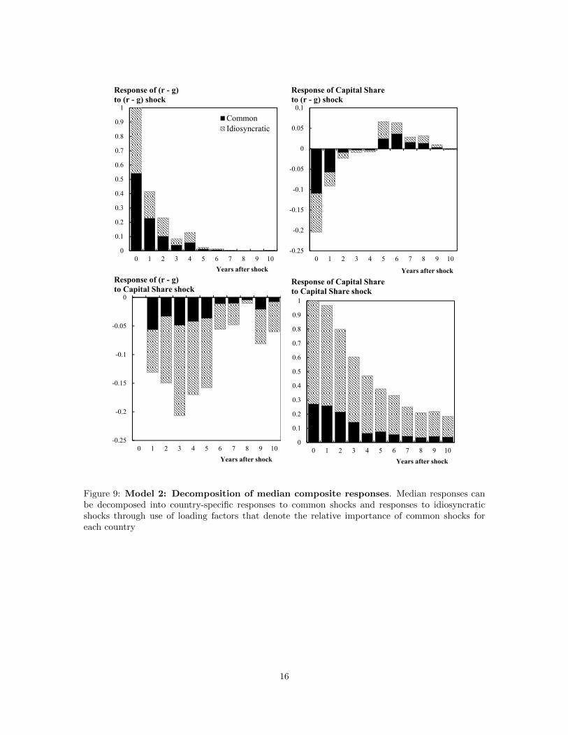
I then turn to Model 2, which checks the relationship between r− g and the capital share. Theresults are less clear cut than with Model 1. However, in the first two years, for at least 75% ofthe countries capital share responds (mildly) negatively to positive shocks to r− g, with the mediangoing from negative to slightly positive then approaching zero asymptotically (see Figure 7). Themedian response is not statistically significant (see Figure 8).
The median response of r − g to capital share shocks is negative and statistically significant.This is intuitive since it is possibly reflecting diminishing marginal returns on capital —for any fixedgrowth rate, increased capital shares are likely to decrease returns and hence drive r−g down. Whencompared to Model 1, idiosyncratic shocks are more dominant (see Figure 9).
p
Figure #. Country Name: Title, Date
Source:
0
0.1
0.2
0.3
0.4
0.5
0.6
0.7
0.8
0.9
1
1.1
0 1 2 3 4 5 6 7 8 9 10
Interquartile rangeMedianAverage
Response of (r - g)to a (r - g) shock
Years after shock
-0.4
-0.3
-0.2
-0.1
0
0.1
0.2
0.3
0.4
0 1 2 3 4 5 6 7 8 9 10Years after shock
Response of (Share of Capital)to a (r - g) shock
-0.8
-0.6
-0.4
-0.2
0
0.2
0.4
0.6
0 1 2 3 4 5 6 7 8 9 10
Years after shock
Response of (r - g)to a (Share of Capital) shock
0
0.2
0.4
0.6
0.8
1
1.2
1.4
0 1 2 3 4 5 6 7 8 9 10
Years after shock
Response of (Share of Capital) to a (Share of Capital) shock
Figure 7: Model 2: Heterogeneous composite impulse responses across sample. Themedian, averages, and interquartile ranges were calculated from the distribution of IRFs of the 18cross-sections.
14

-0.2
0
0.2
0.4
0.6
0.8
1
0 1 2 3 4 5 6 7 8 9 10
Response of (r - g)to a (r - g) shock
-0.5
-0.4
-0.3
-0.2
-0.1
0
0.1
0 1 2 3 4 5 6 7 8 9 10
95%confidenceinterval
Response of (capital share)to a (r - g) shock
-0.3
-0.25
-0.2
-0.15
-0.1
-0.05
0
0.05
0 1 2 3 4 5 6 7 8 9 10
Response of (r - g)to a (capital share) shock 0
0.2
0.4
0.6
0.8
1
1.2
0 1 2 3 4 5 6 7 8 9 10
Response of (capital share) to a (capital share) shock
Years after shock Years after shock
Years after shock Years after shock
Figure 8: Model 2: Median composite responses and confidence intervals. Median responseacross a heterogeneous distribution of IRFs across 18 countries. Confidence intervals calculated froma resampling simulation with 500 repetitions. Since the distribution might change for each repetitionin the simulation exercise, the confidence intervals do not represent the uncertainty around estimatesfor any particular country, but rather for the median estimate of the whole panel.
15
-0.25
-0.2
-0.15
-0.1
-0.05
0
0.05
0.1
0 1 2 3 4 5 6 7 8 9 10
Response of Capital Shareto (r - g) shock
Years after shock
0
0.1
0.2
0.3
0.4
0.5
0.6
0.7
0.8
0.9
1
0 1 2 3 4 5 6 7 8 9 10
Response of Capital Shareto Capital Share shock
Years after shock
0
0.1
0.2
0.3
0.4
0.5
0.6
0.7
0.8
0.9
1
0 1 2 3 4 5 6 7 8 9 10
CommonIdiosyncratic
Response of (r - g)to (r - g) shock
Years after shock
-0.25
-0.2
-0.15
-0.1
-0.05
0
0 1 2 3 4 5 6 7 8 9 10
Response of (r - g)to Capital Share shock
Years after shock
Figure 9: Model 2: Decomposition of median composite responses. Median responses canbe decomposed into country-specific responses to common shocks and responses to idiosyncraticshocks through use of loading factors that denote the relative importance of common shocks foreach country
16
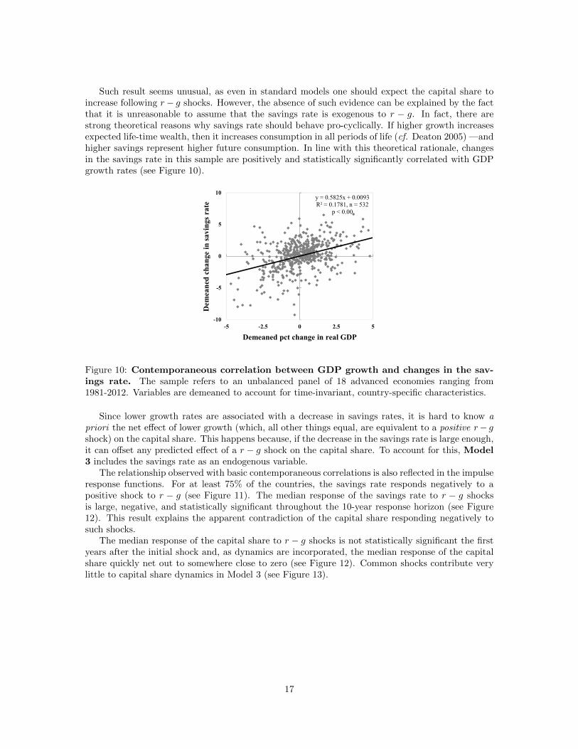
Such result seems unusual, as even in standard models one should expect the capital share toincrease following r− g shocks. However, the absence of such evidence can be explained by the factthat it is unreasonable to assume that the savings rate is exogenous to r − g. In fact, there arestrong theoretical reasons why savings rate should behave pro-cyclically. If higher growth increasesexpected life-time wealth, then it increases consumption in all periods of life (cf. Deaton 2005) —andhigher savings represent higher future consumption. In line with this theoretical rationale, changesin the savings rate in this sample are positively and statistically significantly correlated with GDPgrowth rates (see Figure 10).
y = 0.5825x + 0.0093R² = 0.1781, n = 532
p < 0.00
-10
-5
0
5
10
-5 -2.5 0 2.5 5
Demeaned pct change in real GDP
Dem
eane
d ch
ange
in sa
ving
s rat
e
Figure 10: Contemporaneous correlation between GDP growth and changes in the sav-ings rate. The sample refers to an unbalanced panel of 18 advanced economies ranging from1981-2012. Variables are demeaned to account for time-invariant, country-specific characteristics.
Since lower growth rates are associated with a decrease in savings rates, it is hard to know apriori the net effect of lower growth (which, all other things equal, are equivalent to a positive r− gshock) on the capital share. This happens because, if the decrease in the savings rate is large enough,it can offset any predicted effect of a r − g shock on the capital share. To account for this, Model3 includes the savings rate as an endogenous variable.
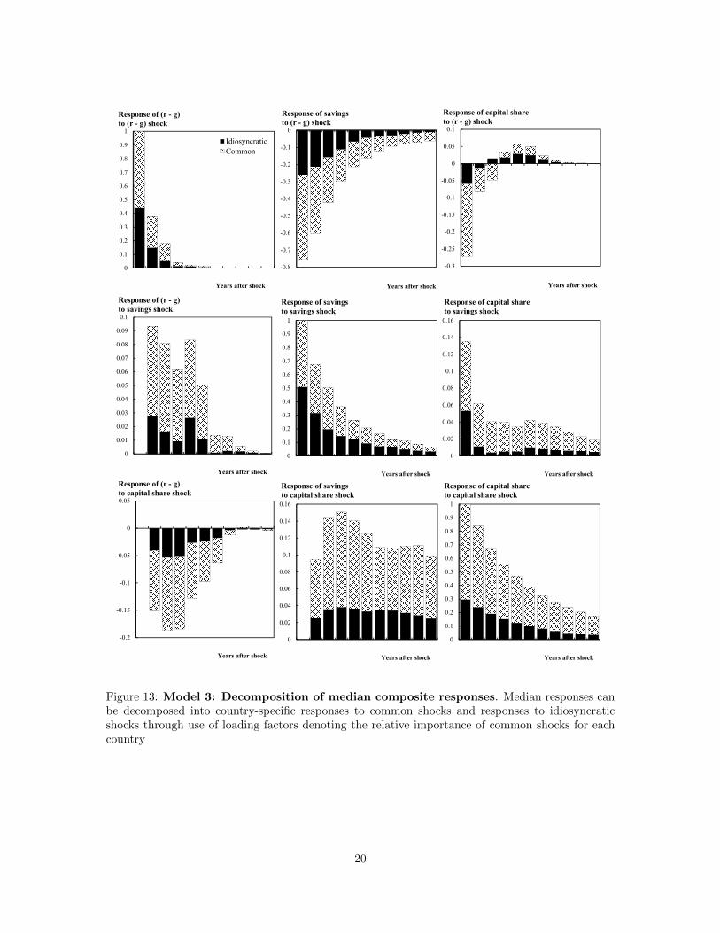
The relationship observed with basic contemporaneous correlations is also reflected in the impulseresponse functions. For at least 75% of the countries, the savings rate responds negatively to apositive shock to r − g (see Figure 11). The median response of the savings rate to r − g shocksis large, negative, and statistically significant throughout the 10-year response horizon (see Figure12). This result explains the apparent contradiction of the capital share responding negatively tosuch shocks.
The median response of the capital share to r − g shocks is not statistically significant the firstyears after the initial shock and, as dynamics are incorporated, the median response of the capitalshare quickly net out to somewhere close to zero (see Figure 12). Common shocks contribute verylittle to capital share dynamics in Model 3 (see Figure 13).
17

Figure #. Country Name: Title, Date
0
0.1
0.2
0.3
0.4
0.5
0.6
0.7
0.8
0.9
1
1.1
0 1 2 3 4 5 6 7 8 9 10
Interquartile rangeMedianAverage
Response of (r - g)to a (r - g) shock
Years after shock
-1.6
-1.4
-1.2
-1
-0.8
-0.6
-0.4
-0.2
0
0.2
0 1 2 3 4 5 6 7 8 9 10Years after shock
Response of (Savings Rate)to a (r - g) shock
-0.3
-0.2
-0.1
0
0.1
0.2
0.3
0.4
0.5
0 1 2 3 4 5 6 7 8 9 10
Years after shock
Response of (r - g)to a (Savings) shock
0
0.2
0.4
0.6
0.8
1
1.2
0 1 2 3 4 5 6 7 8 9 10
Years after shock
Response of (Savings) to a (Savings) shock
-0.5
-0.4
-0.3
-0.2
-0.1
0
0.1
0.2
0.3
0.4
0 1 2 3 4 5 6 7 8 9 10Years after shock
Response of (Capital Share)to a (r - g) shock
-0.25
-0.2
-0.15
-0.1
-0.05
0
0.05
0.1
0.15
0.2
0.25
0.3
0 1 2 3 4 5 6 7 8 9 10
Years after shock
Response of (Share of Capital) to a (Savings) shock
-0.6
-0.4
-0.2
0
0.2
0.4
0.6
0 1 2 3 4 5 6 7 8 9 10
Years after shock
Response of (r - g)to a (Share of Capital) shock
-0.1
0
0.1
0.2
0.3
0.4
0.5
0.6
0 1 2 3 4 5 6 7 8 9 10
Years after shock
Response of (Savings) to a (Share of Capital) shock
0
0.2
0.4
0.6
0.8
1
1.2
0 1 2 3 4 5 6 7 8 9 10
Years after shock
Response of (Share of Capital) to a (Share of Capital) shock
Figure 11: Model 3: Heterogeneous composite impulse responses across sample. Themedian, averages, and interquartile ranges were calculated from the distribution of IRFs of the 18cross-sections.
18

-0.2
0
0.2
0.4
0.6
0.8
1
0 1 2 3 4 5 6 7 8 9 10
Response of (r - g)to a (r - g) shock
-1.5
-1.3
-1.1
-0.9
-0.7
-0.5
-0.3
-0.1
0.1
0 1 2 3 4 5 6 7 8 9 10
95%confidenceinterval
Response of (savings)to a (r - g) shock
-0.05
0
0.05
0.1
0.15
0.2
0.25
0 1 2 3 4 5 6 7 8 9 10
Response of (r - g)to a (savings) shock 0
0.2
0.4
0.6
0.8
1
1.2
0 1 2 3 4 5 6 7 8 9 10
Response of (savings) to a (savings) shock
-1
-0.8
-0.6
-0.4
-0.2
0
0.2
0.4
0 1 2 3 4 5 6 7 8 9 10
Response of (capital share)to a (r - g) shock
-0.4
-0.2
0
0.2
0.4
0.6
0.8
0 1 2 3 4 5 6 7 8 9 10
Response of (capital share) to a (savings) shock
-0.4
-0.35
-0.3
-0.25
-0.2
-0.15
-0.1
-0.05
0
0.05
0.1
0 1 2 3 4 5 6 7 8 9 10
Response of (r - g)to a (capital share) shock -0.2
-0.1
0
0.1
0.2
0.3
0.4
1 2 3 4 5 6 7 8 9 10 11
Response of (savings)to a (capital share) shock
0
0.2
0.4
0.6
0.8
1
1.2
0 1 2 3 4 5 6 7 8 9 10
Response of (capital share) to a (capital share) shock
Years after shock Years after shock
Years after shock Years after shock
Years after shock
Years after shock
Years after shock Years after shock Years after shock
Figure 12: Model 3: Median composite responses and confidence intervals. Median re-sponse across a heterogeneous distribution of IRFs of 18 countries. Confidence intervals calculatedfrom a resampling simulation with 500 repetitions. Since the distribution might change for each rep-etition in the simulation exercise, the confidence intervals do not represent the uncertainty aroundestimates for any particular country, but rather for the median estimate of the whole panel.
19
-0.3
-0.25
-0.2
-0.15
-0.1
-0.05
0
0.05
0.1
Response of capital shareto (r - g) shock
Years after shock
0
0.1
0.2
0.3
0.4
0.5
0.6
0.7
0.8
0.9
1
Response of savingsto savings shock
Years after shock
0
0.1
0.2
0.3
0.4
0.5
0.6
0.7
0.8
0.9
1IdiosyncraticCommon
Response of (r - g)to (r - g) shock
Years after shock
0
0.01
0.02
0.03
0.04
0.05
0.06
0.07
0.08
0.09
0.1
Response of (r - g)to savings shock
Years after shock
-0.8
-0.7
-0.6
-0.5
-0.4
-0.3
-0.2
-0.1
0
Response of savingsto (r - g) shock
Years after shock
0
0.02
0.04
0.06
0.08
0.1
0.12
0.14
0.16
Response of capital shareto savings shock
Years after shock
0
0.02
0.04
0.06
0.08
0.1
0.12
0.14
0.16
Response of savingsto capital share shock
Years after shock
-0.2
-0.15
-0.1
-0.05
0
0.05
Response of (r - g)to capital share shock
Years after shock
0
0.1
0.2
0.3
0.4
0.5
0.6
0.7
0.8
0.9
1
Response of capital shareto capital share shock
Years after shock
Figure 13: Model 3: Decomposition of median composite responses. Median responses canbe decomposed into country-specific responses to common shocks and responses to idiosyncraticshocks through use of loading factors denoting the relative importance of common shocks for eachcountry
20

6 Robustness
I run several alternative specifications to check the robustness of results. I do that by modifyingbaseline Models 1 and 3. I present all alternative results in Figure 14.
-0.4
-0.3
-0.2
-0.1
0
0.1
0.2
0.3
0.4
0 1 2 3 4 5 6 7 8 9 10
BaselineWithout taxes (alternative)Short term yields (alternative)Implied r (alternative)Inverted cholesky ordering (alternative)
Response of (share of top 1%)to a (r - g) shock
Years after shock
-0.4
-0.3
-0.2
-0.1
0
0.1
0.2
0.3
0.4
0 1 2 3 4 5 6 7 8 9 10
BaselineWithout taxes (alternative)Short term yields (alternative)Implied r (alternative)Inverted cholesky ordering (alternative)
Response of (capital share)to a (r - g) shock
Years after shockYears after shockYears after shock
Figure 14: Robustness checks - re-estimation of Models 1 and 3: Median compositeresponses. This figure compares median responses across a distribution of IRFs of 19 (Model 1) /18 (Model 3) countries using different specifications.
First I run an alternative model ignoring tax rates. Tax rates are important for inequality, aspointed out by Piketty and Saez (2013), but it could be that deducting tax rates from returns isadding noise to the results. However, when re-estimating the models without taking taxes intoaccount, the results are similar to the baseline. The median responses of the share of the top 1% tor − g shocks are still negative, albeit less negative than in Model 1.
When replacing long-term bond yields with short term yields (usually central bank policy rates),median responses are very similar to the baseline for the initial response horizons. In outer years,responses net out to zero faster than in the baseline.
I then re-estimate the models using an implied measure of r from the national accounts. Derivingthis measure is straightforward. Since capital share is the return on capital times the capital-to-income ratio (α = rK/Y ), it follows that the return on capital is the capital share divided by thecapital-to-income ratio (r = αY/K). After calculating implied returns on capital for all countriesfrom the Penn World Tables, I deducted growth rates and re-estimated Model 1. Median responsesstill behave in a comparable fashion to all other specifications.
Overall, the results are rather robust to different measures of r. There is no evidence that theshare of the top 1% responds positively to increases in r − g spread.
Similarly, for the capital share, despite small differences, the results are virtually the same asin Model 3 —with the savings rate playing a counter-balancing role after r − g shocks and mediancapital share responses going from slightly negative to slightly positive before converging towardszero.
Finally, I re-run both models with an inverted Cholesky ordering, i.e. with the share of the top 1%and the share of capital in the national income as the most exogenous variable. It could be the casethat the original restrictions imposed on the baseline specifications were hiding a positive effect ofr−g over share of the top 1% and the share of capital. However, in the alternative specification, such
21

effects are very close to zero, which renders them both statistically and economically insignificant.Yet again, in this last alternative specification, there is no evidence in support of Piketty’s hypothesesof r − g increasing the capital share and income inequality.
While baseline conclusions are reasonably robust to all the different specifications estimated,there are several other possible extensions of the empirical models which can provide additionalrobustness to the results. These include, for instance, using the Penn World Table’s estimates oftime-varying depreciation rates, using measures of equity prices as a proxy for the return on capital,incorporating foreign savings to the model, or using a different measure for inequality (such as, forinstance, the Gini coefficient). I intend to pursue some of these in future research.
7 Discussion: What is the Takeaway?
Piketty’s conclusion that inequality will increase in the future rests on the underlying assumptionthat, as growth decreases over time, driving the r − g spread to increase, capital-to-income ratioswill increase. However, the results from Model 2 and Model 3 fail to show robust positive responsesof capital share to shocks in r− g and cast doubt on Piketty’s conjecture. A possible reason for thisis that Piketty could be underestimating diminishing returns of capital —thereby overestimatingthe elasticity of substitution between capital and labor, whose empirical estimates tend to be muchlower than what he assumes (cf. Rognlie 2014). This relationship is illustrated in this paper by thenegative median responses of r − g to positive capital share shocks.
Another less emphasized but equally important problem with Piketty’s conjecture is highlightedby Krusell and Smith (2015), who argue that Piketty’s predictions are grounded on a flawed theoryof savings —namely, that the savings rate net of depreciation is constant —which exacerbates theexpected increase in capital-to-income ratios as growth rates tend to zero. They present an alter-native model in which agents maximize inter-temporal utility and arrive in a setting in which, onan optimal growth path, the savings rate is pro-cyclical. By showing that the savings rate respondsnegatively to negative growth shocks (which, in turn, are translated into positive r−g shocks) for atleast 75% of the countries in the sample, the results of Model 3 provide empirical support to Kruselland Smith’s analysis.
Piketty (2012) says in his online notes: “with g = 0%, we’re back to Marx apocalyptic con-clusions,” in which capital share goes to 100% and workers take home none of the output. Whilethis is logically consistent with the model’s assumptions, empirically there seem to be endogenousforces preventing that: non-negligible diminishing returns on capital and pro-cyclical changes in thesavings rate. These are two different ways in which the transmission mechanism from r − g to thecapital share might get stuck: with the former, at the limit the rate of return on capital tends to zeroand there is no dynamic transmission; with the latter, if growth approaches zero, the savings mightultimately become zero, offsetting any effect of lower growth on capital share. They are, however,fundamentally different: the first regards the production function and technological change, whilethe second has to do life-cycle behavior of capital owners.
Regarding inequality, the results from Model 1 contradict Piketty’s prediction stating that follow-ing exogenous shocks in r− g inequality should increase. In fact, for at least 75% of the countries inthe sample, the result is negative. These findings are in line with previous results by Acemoglu andRobinson (2015), who found negative coefficients in single-equation panel models when regressingr− g on the share of the top 1%. This paper goes further, not only because the model takes all vari-ables as endogenous, but also because it incorporates tax variability across countries. Additionally,by decomposing between common and idiosyncratic shocks, rather than using time dummies, Model1 does not throw away potentially important information about the effect of structural forces (e.g.,globalization) on these dynamics —which, as Milanovic (2014) argues, is a problem with Acemogluand Robinson’s analysis.
The fact that a positive r − g spread does not lead to higher inequality is not necessarily sur-
22

prising. As illustrated by Mankiw (2015) through a standard model that incorporates taxation anddepreciation, even if r > g, one can arrive in a steady state inequality which does not evolve intoan endless inegalitarian spiral. Milanovic (2017, forthcoming) explains that the transmission mech-anism between r > g and higher income inequality requires all of the following conditions to hold:(a) savings rates have to be sufficiently high; (b) capital income needs to more unequally distributedthan labor income; and (c) a high correlation between drawing capital income and being on the topof the income distribution. In a dynamic fashion, this paper shows that this mechanism is gettingstuck because the negative responses of the savings rate to r − g shocks violate the first condition,thereby preventing higher levels inequality when compared to those observed before the increases inr − g.
Since estimated dynamics do not confirm Piketty’s theory, observed income inequality in manyadvanced economies over the past decades are probably explained by factors other than the spreadbetween r and g. In fact, there is evidence that recent inequality trends are not related to thedistribution of national income between factors of production but primarily to the rising inequal-ity of labor income (cf. Francese and Mulas-Granados 2015). Indeed, there are many potentialexplanations for the rising labor income inequality —as, for instance:
• Dabla-Norris et al. (2015), after evaluating cross-country evidence, find that past changes ininequality in advanced economies are associated the most with two labor market changes:higher skill premia and lower union membership rates. Jaumotte and Buitron (2015) alsopresent results that correlate changes in labor market institutions, particularly lower uniondensity, with increases in income inequality in advanced economies.
• Aghion et al. (2015) suggest innovation plays a significant role. If innovators are rewardedwith higher incomes due to a temporary technological advantage (in a Schumpeterian fashion),inequality would be exacerbated. The authors show that innovation explains about a fifth ofthe higher inequality observed in the U.S. since 1975.
• Mare (2016) and Greenwood et al. (2012) argue that changes in mating behavior helped ex-acerbate income inequality. The probability that someone will marry another person with asimilar socio-educational background (labeled “assortative mating”) increased in tandem withthe rise in income inequality in U.S. in the recent decades. The interaction between higherskill premia and higher assortative mating exacerbates household income inequality, becausethe gap between higher and lower earners became larger and couples became more segregated.
• Chong and Gradstein (2007) use a dynamic panel to show inequality tends to decrease as insti-tutional quality improves. The underlying logic is that if the basic rules of economic behaviorare not symmetrically enforced, the rich will have a higher chance to extract economic rents,thereby increasing inequality. Acemoglu and Robinson (2015) make a similar argument. Theysay that economic institutions affect the distribution of skills in society, indirectly determininginequality patterns.
None of the evidence provided in the papers listed above is definite or mutually exclusive. Rather,they are most likely complementary explanations for the recent developments of a complex phe-nomenon such as income inequality. But what they do have in common is that none of them pointto capital-to-income or r − g dynamics as the driving causes of inequality patterns.
Some years after the publication of Capital, Piketty (2015) himself recognized the “rise in laborincome inequality in recent decades has evidently little to do with r − g, and it is clearly a veryimportant historical development.” He nonetheless emphasized that a higher r − g spread will beimportant and will exacerbate future inequality changes.
However, the results in this paper show that this is likely not to be the case. The resultscorroborate the idea that recent inequality changes are not explained by r − g but also that newshocks to r − g will likely not lead to higher inequality, as there is no evidence that shocks to r − g
23

increase income inequality. Combined, the observed endogenous dynamics of r− g and the share ofthe top 1% and the capital share, respectively, cast doubt on the reasonability of Piketty’s predictionabout inequality trends.
A potential caveat of this analysis is that its sample size might be too short to capture thelong run relationship under scrutiny. While this is certainly possible, there are some limits to suchcriticism. First, since the focus of the exercise are advanced countries, one expects them to beclose to their respective steady states. In such case, it is more likely that the thirty year sampleis enough to capture the steady states and the effect of shocks that disturb such steady states.Second, Acemoglu and Robinson (2015) run single-equation models using 10- and 20-year averagesgoing back all the way to the 1800s and find no statistically significant evidence that increases inr − g positively impact the share of the top 1% in the national income. Unfortunately, using thosemulti-decennial averages in a endogenous dynamic panel framework would render the identificationrestrictions so strong (namely, that one variable has no impact over the other for 20 years) that itwould make the entire exercise futile.
8 Conclusions
The purpose of this paper is very Popperian in nature: it tests interesting, logically consistent, andfalsifiable hypotheses. Thereby, it contributes to the literature by checking the empirical veracity ofa very influential theory regarding income inequality patterns.
In doing so, I found no evidence to corroborate the idea that the r−g gap drives the capital sharein national income. There are endogenous forces overlooked by Piketty —particularly the cyclicalityof the savings rate —which balance out predicted large increases in the capital share. On inequality,the evidence against Piketty’s predictions is even stronger: for at least 75% of the countries, theresponse of inequality to increases in r − g has the opposite sign to that postulated by Piketty.
These results are robust to different calculations of r− g. Regardless of taking the real return oncapital as long-term sovereign bond yields, short-term interest rates or implied returns from nationalaccounting tables, the dynamics move in the same direction. Additionally, including or excludingtaxes does not alter the qualitative takeaways from the results either.
Knowing if increases r − g lead to inequality is very important, not only for economics as ascience of human action but also for the policy repercussions of such conclusions. Without knowingthe underlying causes of such trends, it is impossible to design policy actions to counter them.
Inequality is a complex phenomenon and its trends are very sluggish. It is certainly possible thatthe long terms relationships Piketty proposes exist and are simply not captured by the 30 years ofdata for the 19 advanced economies included in this sample. However, the best available data showthat, if one is looking to potential solutions to increasing income inequality, one should not focus onr − g, but elsewhere.
References
Acemoglu, Daron and James A. Robinson (2015). “The Rise and Decline of General Laws of Capi-talism”. In: Journal of Economic Perspectives 29.1, pp. 3–28. doi: 10.1257/jep.29.1.3.
Aghion, Philippe et al. (2015). Innovation and Top Income Inequality. Working Paper 21247. Na-tional Bureau of Economic Research. doi: 10.3386/w21247.
Causa, Orsett and Asa Johansson (2013). “Intergenerational social mobility in OECD countries”.In: OECD Journal: Economic Studies 2010.1, pp. 1–44. issn: 1468-2362.
Chong, Alberto and Mark Gradstein (2007). “Inequality and Institutions”. In: The Review of Eco-nomics and Statistics 89.3, pp. 454–465. doi: 10.1162/rest.89.3.454.
Corak, Miles (2016). Inequality from Generation to Generation: The United States in Comparison.Discussion Paper 9929. Institute for the Study of Labor (IZA).
24

Dabla-Norris, Era et al. (2015). Causes and Consequences of Income Inequality: A Global Perspective.IMF Staff Discussion Note 15/13. International Monetary Fund. doi: 10.5089/9781513555188.006.
Deaton, Angus S. (2005). “Franco Modigliani and the Life Cycle Theory of Consumption”. In: BancaNazionale del Lavoro Quarterly Review 58.233-234, pp. 91–108.
Francese, Maura and Carlos Mulas-Granados (2015). Functional Income Distribution and Its Rolein Explaining Inequality. IMF Working Paper 15/244. International Monetary Fund. doi: 10.5089/9781513549828.001.
Greenwood, Jeremy et al. (2012). Technology and the Changing Family: A Unified Model of Marriage,Divorce, Educational Attainment and Married Female Labor-Force Participation. Working Paper17735. National Bureau of Economic Research. doi: 10.3386/w17735.
Jaumotte, Florence and Carolina Osorio Buitron (2015). Inequality and Labor Market Institutions.IMF Staff Discussion Note 15/14. International Monetary Fund. doi: 10.5089/9781513577258.006.
Krusell, Per and Anthony Smith (2015). “Is Piketty’s ‘Second Law of Capitalism’ Fundamental?”In: Journal of Political Economy 123.4, pp. 725–748. doi: 10.1086/682574.
Lutkepohl, Helmut (2007). New Introduction to Multiple Time Series Analysis. Berlin: Springer.Mankiw, Greg (2015). “Yes, r > g. So What?” In: American Economic Review: Papers & Proceedings
105.5, pp. 43–47. doi: 10.1257/aer.p20151059.Mare, Robert D. (2016). “Educational Homogamy in Two Gilded Ages: Evidence from Inter-generational
Social Mobility Data”. In: The ANNALS of the American Academy of Political and Social Science663.1, pp. 117–139. doi: 10.1177/0002716215596967.
Milanovic, Branko (2014). My take on the Acemoglu-Robinson critique of Piketty. http://glineq.blogspot.com/2014/08/my-take-on-acemoglu-robinson-critique.html. Accessed: 11-Feb-2016.
— (2017, forthcoming). “Increasing capital income share and its effect on personal income inequal-ity”. In: After Piketty’s “Capital in the 21st century”: The agenda for fighting inequality. Ed. byHeather Boushey, Bradford DeLong, and Marshall Steinbaum. Cambridge: Harvard UniversityPress.
Pedroni, Peter (2013). “Structural Panel VARs”. In: Econometrics 1, pp. 180–206. doi: 10.3390/econometrics1020180.
Pesaran, M Hashem and Ron Smith (1995). “Estimating long-run relationships from dynamic het-erogeneous panels”. In: Journal of Econometrics 68.1, pp. 79–113. doi: 10.1016/0304-4076(94)01644-F.
Piketty, Thomas (2012). ”Economics of Inequality. Course Notes: Models of Growth & Capital Accu-mulation. Is Balanced Growth Possible?”. http://piketty.pse.ens.fr/fr/teaching/10/25.Accessed: 11-Feb-2016.
— (2014). Capital in the Twenty-First Century. Cambridge: Harvard University Press.— (2015). “About Capital in the Twenty-First Century”. In: American Economic Review: Papers
& Proceedings 105.5, pp. 48–53. doi: 10.1257/aer.p20151060.Piketty, Thomas and Emmanuel Saez (2013). “A Theory of Optimal Inheritance Taxation”. In:
Econometrica 81.5, pp. 1851–1886. doi: 10.3982/ECTA10712.Piketty, Thomas and Gabriel Zucman (2015). “Wealth and Inheritance in the Long Run”. In: Hand-
book of Income Distribution, v. 2A. Ed. by Jan Fagerberg, David C. Mowery, and Richard R.Nelson. Amsterdam: North Holland. Chap. 15, pp. 1303–1368. doi: 10.1016/B978- 0- 444-59429-7.00016-9.
Rognlie, Matthew (2014). A note on Piketty and diminishing returns to capital. http://www.mit.edu/~mrognlie/piketty_diminishing_returns.pdf. Accessed: 11-Feb-2016.
25

A Appendix: Data and Sources
A.1 Countries Sample
Samples are slightly different in Model 1 compared to Models 2 and 3 to account for dynamic(in)stability in different samples.
Sample for Model 1: Australia, Canada, Finland, France, Germany, Italy, Ireland, Japan,Korea, Netherlands, New Zealand, Norway, Portugal, Singapore, Spain, Sweden, Switzerland, theUnited Kingdom, and United States.
Sample for Models 2 and 3: Australia, Canada, Denmark, Finland, France, Italy, Japan,Korea, Netherlands, New Zealand, Norway, Portugal, Singapore, Spain, Sweden, Switzerland, theUnited Kingdom, and United States.
A.2 Data Sources
Variable Scale SourceShare of the top 1% Percent of national income World Top Income DatabaseCapital share Percent of national income Penn World TablesReal GDP growth Annual percent change World Economic OutlookGDP deflators Index World Economic OutlookGross national savings Percent of national income World Economic OutlookCorporate income tax rates Percent OECD’s Tax Database10-YR sovereign bond yields Percent Bloomberg & Haver AnalyticsShort-term interest rates Percent Haver Analytics & IMFImplied return on capital Percent Derived from Penn World Tables
26

B Appendix: Standard Error Simulation Algorithm
Before starting the simulation, I run the individual VARs in equation (7) and collect predicted values(yi,t) and reduced form residuals (ei,t). I then transform reduced-form residuals into their structuralequivalents (ui,t = B−1i ei,t) and run the following algorithm:
1. I follow these steps k = 500 times:
(a) I re-sample the structural residuals. Let ui,t denote re-sampled structural residuals ui,t.
(b) I then transform re-sampled structural residuals back into reduced-form residuals bymultiplying them with B: ei,t = Biui,t.
(c) I sum the predicted values of y∗i,t and re-sampled residuals to create pseudo-series for allmembers M . Let the pseudo-series be yi,t ≡ yi,t + ei,t.
(d) I re-estimate the model with the pseudo-series: Biyi,t = A(L)yi,t−1 + ei,t.
(e) I collect the matrices of responses, extract individual vectors for each pseudo-IRF, orga-nize them into a matrix, and calculate the median response of this distribution.
(f) If this repetition < k, I go back to (a), otherwise, I move to step 2.
2. After I repeat this procedure k times the result will be a set of distribution matrices D ofsimulated medians:
Dm =
ρ11m . . . ρk1m...
. . ....
ρ1hm . . . ρkhm
hxk
(B.1)
where m is the mth response variable, h is the response horizon, and k is the number ofrepetitions of the simulation exercise.
3. From Dm I take square root of the second moment of each row to build a vector of standarderrors:
σρm =
Var[{ρ11m, . . . , ρk1m}]1/2...
Var[{ρ1hm, . . . , ρkhm}]1/2
hx1
(B.2)
27