Kernel estimation and display of a five-dimensional … estimation and display of a five-dimensional conditional intensity function G. Adelfio Dipartimento di Scienze Statistiche

Nonlin. Processes Geophys., 17, 237–244, 2010www.nonlin-processes-geophys.net/17/237/2010/© Author(s) 2010. This work is distributed underthe Creative Commons Attribution 3.0 License.

Nonlinear Processesin Geophysics

Kernel estimation and display of a five-dimensional conditionalintensity function

G. Adelfio

Dipartimento di Scienze Statistiche e Matematiche “Silvio Vianelli”, University of Palermo, Palermo, Italy

Received: 3 December 2009 – Revised: 29 January 2010 – Accepted: 8 February 2010 – Published: 22 April 2010

Abstract. The aim of this paper is to find a convenient andeffective method of displaying some second order propertiesin a neighbourhood of a selected point of the process. Theused techniques are based on very general high-dimensionalnonparametric smoothing developed to define a more gen-eral version of the conditional intensity function introducedin earlier earthquake studies byVere-Jones(1978).

1 Introduction

This paper is concerned with the second order properties of amultidimensional point process in contexts where some fea-tures of a given point (e.g. location, depth, magnitude) playa dominant role in determining the local behavior of the pro-cess in a neighbourhood of the selected point. The aim ofthe paper is to describe a convenient and effective method ofdisplaying second order properties of counts in a neighbour-hood of a selected point of an observed point process and toexamine how those properties are affected by the features ofthe fixed point. In particular we would like to display secondorder properties of counts in a neighbourhood of the initialevent in an aftershock sequence or swarm in a seismic activearea. For instance, the way these properties change with themagnitude of the initial event tells us something about thephysical processes governing the numbers and distributionsof the aftershocks respond to the size of the initial event.Similar issues arise in the discussion of medical epidemicdata, where the size and severity of the epidemic overall maybe related to characteristics of the initial recorded infection.

To look at second order properties, the counts need to beaveraged over both the choice of a selected point and overthe events in its neighbourhood. Ripley’s K-function (Ripley,

Correspondence to:G. Adelfio([email protected])

1976) is commonly used for such a purpose in discussing thecumulative behavior of interpoint distances about an initialpoint. It is defined as the expected number of events fallingwithin a given distanceδ of the initial event, divided by theoverall density (rate in 2-dimensions) of the process, sayλ.Since it is defined as an average over many initial points, theK-function cannot be used to distinguish processes with thesame (average) second order properties. As an alternative,Getis and Franklin(1987) suggested examining the behaviorof the occurrence patterns in the neighbourhood of selectedinitial points developing a second order neighbor analysis ofmapped point patterns. However, this method is not use-ful for determining whether a given pattern is random, clus-tered or regular (Doguwa, 1989). Adelfio and Schoenberg(2009) suggested using a weighted version of some secondorder statistics to provide diagnostic tests. InAdelfio andChiodi (2009) weighted second order statistics are used toassess the fitting of seismic models to real catalogs.Gril-lenzoni(2006) focussed on the conditional intensity functionof a space-time process, where conditioning is made on thebasis of past events only.

Second order statistics, such as the Ripley’s K-function(Ripley, 1976), are useful to describe observed point patternscharacterized by high correlation structures both in space andtime and are also designed to test the randomness hypoth-esis often based on the Poisson distribution. For this rea-son second order statistics are crucial to study and compre-hend seismic process and its realization, since description ofseismic events often requires the definition of more complexmodels than stationary Poisson process and the relaxationof any assumption about statistical independence of earth-quakes. Indeed, a more realistic description of seismicity of-ten needs the study and the interpretation of features like self-similarity, long-range dependence and fractal dimension.

Published by Copernicus Publications on behalf of the European Geosciences Union and the American Geophysical Union.

http://creativecommons.org/licenses/by/3.0/

238 G. Adelfio: Kernel estimation of a five-dimension conditional intensity function

In this paper a nonparametric estimation of the second or-der conditional intensity function (CIF) introduced byVere-Jones(1978) is provided, by making use of kernel intensityestimators. The nonparametric second order CIF is here in-troduced to analyze the influence in a neighbourhood of amultidimensional point to some properties of the observedpoint pattern, by using a procedure that does not require anyconstraining assumption to characterize the generating pro-cess.

In Sect.2 a brief introduction of spatial-temporal pointprocesses and their second order characteristics is pro-vided. The proposed nonparametric approach is introducedin Sect.3, showing some application in Sect.4. Section5provides some concluding remarks and directions for futurestudy.

2 Point processes and conditional intensity function

A spatial-temporal point process is a random point patterndefined by time and location of every single event. Pointprocesses are here introduced by a mathematical approachthat uses the definition of a counting measure on a setX ⊆

Rd ,d ≥ 1, with positive values inZ: for each Borel setBthis Z+-valued random measure gives the number of eventsfalling in B.

This section reviews some basic definitions related to pointprocesses, reported to introduce the notation used throughoutthe paper. For further elaboration and references, please seeDaley and Vere-Jones(2003).

Definition 1 Point process

Let (�,A,P ) be a probability space and8 a collection oflocally finite counting measures onX ⊂ Rd . DefineX as theBorelσ -algebra ofX and letN be the smallestσ -algebra on8, generated by sets of the form{φ ∈ 8 : φ(B) = n} for allB ∈X . A point processN onX is a measurable mapping of(�,X ) into (8,N ). A point process defined over(�,A,P )

induces a probability measure5N (Y ) = P(N ∈ Y ),∀Y ∈N(Cressie, 1991).

Given a point processN defined on the space(X,X ) anda Borel setB, the number of pointsN(B) in B is a randomvariable with first moment defined by:

µN (B) = E[N(B)] =

∫8

φ(B)5N (dφ)

that is a measure on(X,X ). The measureµN is called themean measure or first moment measure ofN (Cressie, 1991).The second moment measure ofN is given by:

µ(2)N (B1·B2) = E[N(B1)N(B2)] =

∫8

φ(B1)φ(B2)5N (dφ),

with B1,B2 ∈X . If it is finite in X (2) the process is secondorder.

Let ds anddu be small regions located ats andu ∈ X,and let`(x) be the Lebesgue measure ofx. Thefirst orderintensityis defined by:

η(s) = lim`(ds)→0

µN (ds)

`(ds);

thesecond order intensityis defined by:

η2(s,u)= lim`(ds)→ 0`(du) → 0

µ(2)N (ds ·du)

`(ds)`(du).

The second-order counting properties of such a processcan be summarized by acovariance density:

c(s,u)ds du = Cov{N(ds),N(du)}, (s 6= u). (1)

The covariance measure also has a singular componentconcentrated along the lines = u, as illustrated by the for-mula:

Var{N(ds)} = E [N(s)] = µN (s).

Let N be a point process on a spatial-temporal domainX =

R+ ×Rd , d ≥ 2; the functionλ∗(t,z) = λ(t,z|Ht ), definedby:

λ∗(t,z) = lim`(dt) → 0`(dz) → 0

E [N([t,t +dt ) · [ z,z+dz) | Ht )]

`(dt)`(dz),

(2)

is the intensity function of the process conditioned toHt ,that is the space-time occurrence history of the process up totime t , or in other words, theσ -algebra of events occurring attimes up to but not includingt ; dt,dz are time and space in-crements respectively, andE[N([t,t +dt)×[z,z+dz)|Ht )]

is the history-dependent expected value of occurrence inthe volume{[t,t + dt) × [z,z + dz)}. The conditional in-tensity function is a function of the point history and itis itself a stochastic process depending on the past up totime t . Assuming such a limit exists for each point(t,z)

in the space-time domain and the point process is simple,the conditional intensity process uniquely characterizes thefinite-dimensional distributions ofN (Daley and Vere-Jones,2003). According to the used notation, the star inλ∗(·) isused to indicate that the intensity is a function of the pasthistoryHt .

If the conditional intensity function is independent of thepast history and dependent only on the current time and spa-tial location, Eq. (2) determinesλ(t,z) and identifies an inho-mogeneous Poisson process. A constant conditional intensityprovides a stationary Poisson process.

Nonlin. Processes Geophys., 17, 237–244, 2010 www.nonlin-processes-geophys.net/17/237/2010/

G. Adelfio: Kernel estimation of a five-dimension conditional intensity function 239

In a time-stationary but spatially inhomogeneous process,the expression in (2) is:

λ∗(t,z) = λf ∗(z)

with λ the overall rate occurrence for a given region andf (·)

a time-invariant space density. A more general form for (2)is provided assuming a separable form, in which the spatialterm is assumed to be univariate in time and temporal densityis not constant, where the both terms are allowed to dependon the past history, such that:

λ∗(t,z) = λ∗(t)f ∗(z) (3)

It simplifies to the product of constants for homogeneousPoisson processes.

In this paper a nonparametric estimation of a second or-der measure like (3) is provided to describe dependencystructures of a multidimensional observed seismic process byusing a flexible procedure based on kernel intensity estima-tors.

3 Nonparametric estimation

For an adequate description of the seismic activity of a fixedarea and to suggest useful ideas on the mechanism of a suchcomplex process, the definition of a valid and effective modelis required. When a complete definition of a parametricmodel is not reliable, nonparametric approach could be use-ful. Indeed, in seismic modelling contexts, parametric mod-els are not always useful since the definition of a reliablemathematical model from the geophysical theory may not beavailable.

In general, some disadvantages of the parametric mod-elling can be avoided by using flexible procedures (nonpara-metric techniques), based on kernel intensity methods (Sil-verman, 1986). Given n observed eventss1,s2...,sn in ad-dimensional given region, the kernel estimator of an un-known densityf in Rd is defined as:

f (s1,...,sd;h) =1

nhs1 ...hsd

n∑i=1

K

(s1−si1

hs1

,...,sd−sid

hsd

)(4)

where K(s1,...,sd) denotes a multivariate kernel density(usually the standard Normal density function) operating ond arguments centered at(si1,...,sid) andh=(hs1,...,hsd)

′ isthe vector of the smoothing parameters of the kernel func-tions. If si = {ti,xi,yi,zi,Mi}, the space-time-magnitudekernel intensity estimator of (2) is defined by the superpo-sition of the separable kernel densities:

λ(t,x,y,z,M;h) ∝

n∑i=1

Kt

(t − ti

ht

)· Ks

(x −xi

hx

,y −yi

hy

,z−zi

hz

)KM

(M −Mi

hM

)(5)

whereKt, Ks andKM are temporal, spatial and magnitudekernel density functions, as in (4), respectively.

Introducing the estimator defined in (5), the estimation ofa complex intensity function dependent on the past historyof the process as in (2) now reduces to the estimation of theintensity function of an inhomogeneous Poisson process, in-dependent of the past history and identified by a space-timeGaussian kernel intensity (Adelfio and Ogata, 2010); this re-sult provides useful directions for a simpler estimation ap-proach in describing very complex phenomena such as theseismic one. Separability of time and space kernel densi-ties is here assumed for computational convenience, becauseof the high dimensional issue, although tests to assess thisassumption could be used (Schoenberg, 2004). It might beuseful to note that this assumption is not directly extended tothe intensity function of the process since it is obtained bythe superposition of these densities.

In this context the problem of choosing the amount ofsmoothing is of crucial importance, since smoothing parame-ter regularizes the trade-off between variance and bias of theestimator, that is between random and systematic error. InAdelfio et al. (2006) the seismicity of the Southern Tyrrhe-nian Sea is described by Gaussian kernels and the optimumvalue ofh is chosen such as to minimize the mean integratedsquare error (MISE) of the estimatorf (·). In particular theauthors used the valuehopt that Silverman(1986) obtainedminimizing the MISE off (·) assuming multivariate normal-ity.

In Adelfio (2010) a variable bandwidth procedure is in-troduced, choosinghj

= (hjx,h

jy,h

jt ), i.e. the bandwidth for

thej -th event,j = 1,...,n, as the radius of the smallest cir-cle centered at the location of thej -th event(xj ,yj ,tj ) thatincludes at least a fixed number of further events.

In Adelfio and Ogata(2010) a naive likelihood cross-validation function is optimized to obtain the bandwidth ofthe smoothing kernel used to estimate the intensity for earth-quake occurrence of northern Japan.

Although the use of variable bandwidth may be preferableto reflect local occurrence rates instead of using fixed band-width, in this paper constant smoothing is considered as aconvenient approach to deal with the high dimensionality ofthe analyzed problem.

3.1 Conditional intensity estimation

Conditional intensity estimation can be considered as a gen-eralization of regression, focussing on the estimation of thefull conditioned distribution and not just on the expectationvalue.

www.nonlin-processes-geophys.net/17/237/2010/ Nonlin. Processes Geophys., 17, 237–244, 2010


A discrete estimate of the second order conditional inten-sity for a point process is given byVere-Jones(1978). Nowwe are looking for a smoothed version of the conditional in-tensity, that is the local intensity of the process atp, giventhe occurrence of a point of the process ats. Thus:

h(p|s)dp = E [N(dp)|N(ds) = 1] (6)

wheres andp are points inRd , with d = 5, since we are con-sidering space (3-D), time and magnitude dimensions. Thisfunction can be related to the covariance density (1) by theequation

h(p|s) = µN (p)+c(p,s)/µN (s).

Moreover the formula above can be considered as anotherway of looking at the Ripley’s K-function, useful when theemphasis is on the physical interpretation of the dependence.

In this paper nonparametric kernel estimators are used forestimatingh(p|s) in high-dimensional domain; in this con-text the conditioning puts a different complexion on the prob-lem, as the smoothing parameters have to be adjusted to theconditioning event.

Here we use a version of the conditional intensity func-tion introduced in earlier earthquake studies byVere-Jones(1978), where the second order properties are classified ac-cording to the magnitude of the initial event. In the earlypaper the analysis was based on a crude discretization of theprocess, but in the present paper we make use of kernel den-sity estimates applied jointly to both the conditioning and theconditioned events. More precisely, to evaluate a smoothedversion of the conditional intensity (CIF) in (6), we use theratio estimate

h(p|s) =λ(p,s)

λ(s)(7)

that is, the ratio between the joint intensity of the condition-ing and the conditioned event (i.e.p ands), and the marginalintensity of the conditioning event (events). This functionis therefore estimated as the ratio of the kernel intensity esti-mators, defined in Eq. (5), for λ(p,s) andλ(s), respectively.The kernel estimators consider Gaussian density with zeromean and variance selected in a such way that its standarddeviationh (the kernel bandwidth) minimizes the mean inte-grated square error (MISE) of the estimateλ(·).

This approach simplifies the complex estimation issue ofthe second-order measure in (6), although it implies the useof high dimensional kernel functions. Indeed, the quan-tity in (7) has been computed considering the ratio of five-dimensional kernel estimators, providing, on one hand, avery computer intensive procedure, but on the other hand,some advantages related to the possibility of describing themain features of the process in multiple domains withoutconstraining data to binding assumptions.

Longitude

Latit

ude −43

−42

−41

−40

−39

−38

−37

**

*

**

****

**

*

** **

*

*

** *

*

*

**

**

**

* **

*

*

*

**

*

*

**

*

*

**

*

*

**

*

* *

**

* **

**

* ***

*

*

**

**

**

*

**

*** * *

*

**

*****

* ***

**

*

**

*

****

***** *

*

*

**

*

*

*

***

***

*

**

*

*

**

*

**

** *

**

*

*

*

*

*

***

*

****

**************************************************

*** ** **

* **

*

**

*****

*

**

*

*

**

***

*

**

*

*

*

**

****

* *

******

*

**

*

*

*

*

*

*

** *

*

*

**

***

*

**

**

** *

**

*

*

******

*

**

*

*****

*

*

** *

*

** *

*

**

***

**

**

*

*

*

*

*

**

***

*

** * **

*

***

*

*

*

*

***

*

**

****

*

*

*

***

*

** **

*

**

******

****

*

* *

*

*

*

*

*

*

*

*

**

*

***********

**

*

* *

*

*

*

***********

************

**

*

**

*

*

***

*

*

*************************** ************************************************************************ *****************************************************

****

*****

**********************************************************************************

*********

*

****

***************

*****

*

*

***********

*

*

*

*

***

***

*

*

*

*

*

*

*

***

**

*

**

****

*

**

*** *

*

**

**

*

*

**

*

*** *

*

*

*

***

*

*****

**

**

**

***

****

**

**

**

*

***

*

**

*

*

* ******

* *

*

*

**

***

***

*** *** *************************

** **

***

**

: Depth (0,12]

172 174 176 178 180

* *

*

* *

* **

** **

*

**

*

*

*

*

* *

*

*

*

**

* **

*

*

**

*

***

**

* *

*

*

*

*

****

**

*

***

*

*

*

*

*

*

*

*

*

** ***

*** *

* **

*

****

*

**

***

** *

*

**

*

*

**

**

*

*

*

**

*

*

*

***

* *

*

*

******

*

*

***

*

**

*

* *

**

***

*

*

*

*

*

*

*

*

**

***

*

*

*

*

*

*

***

* *

**

*

*

*

** **

*

** *

*

*

********

**

*

*

**

* **

*

*

*

*****

** **

**

*

*

* ********

*

**

**

**

*

*

*

* **

**

**

**

*

*

**

*

* ******* ********

***

*

**

*

*

* *

* *

*

*

*

**

**

*

*

*

**

***

**

*

*

**

**

**

**

***

**

*

**

* ****

*

********

* **

**

*

**

* *

**

*

* *

**

*

*

*

*

**

*

*

*

*

***

***

****

*

**

*

**

**

**

** *

*

*

*

*

***

*

*

**

*

*

*

*

****

*

* **

***

* *

**

**

* *

**

*

*

**

*

*

*

* *

*

**

*

*

*

*

***

*

* *

****

*

**

**

*

*

*

**

*

*

***

**

**

**

*

*

*

*

*

*

***

**

**

*

***

*

*

* **

**

*

*

*** *

* *

*

**

**

**

*

***

*

*

****** ********** *

*

********

***

***

*

*

* *

*

**

*

***

*

**

*

*

**

*** ***

***

*

**

*

* *

*

*

*

** *

**

*

**

** ***

*

*

**

**

*

**

**

**

**

** *

* **

*

*

***

*

*

*

**

**

**

**

**

*

*

*

*

*

*

**

*

*

*

**

*

*

* *** *

**

***

*

**

*

*** **

*

* * **

**

** *

*

*

***

*

**

**

*

*

: Depth (12,85]

172 174 176 178 180

* * ** **

*

**

*

**

*

*

***

*

***

**

**

**

*

*

** *

**

***

*

***

**

*

*

**

*

*

**

**

**

*

*

*

**

*

***

*

*

****

*

**

**

****

*

****

*** *

*

* ***** **

*

***

**

**

****

*

**

* **

*

***

* *

*

* *

**

***

**

*

*****

****

**

*

* **

*

** *

** *** **

**

*

*

**

**

**

**

**

**

**

***

*

**

*

**

*** *

*

**

*

***

*

*

**

*

***

*

*

*

*

**

*

**

**

*

**

******

*

*

*

*

** *

*

*

****

*

****

* ****

*

**

*

*

*

*

**

***

*

*

*

*****

*

*

**

**

*

*

***

*

*

****

*

*

*

**

***

*

*

*

**

*

*

****

*

**

***

*

*

*** *

*

**

*

***

**

***

***

**

***

**

**

*

*

*

**

**

*

*

**

**

**

*

**

** ***

* *

**

*

*

**** ***

*

**

*

***

*

**

***

******

*

*

*

**

*

***

* **

**

*******

*

**

**

*

***

***

*

***

*****

***

*******

*

* *

*

***

*

******

**

**

*

***

*******

*

* ***

*

**

***

**

* ***

*

**

***

*

*

*

*

*

*

**

**

***

**

*

**

*

*** ** ***

*

*** *

*

**

**

*

***

*

***

**

***

**

*

***

**

**

**

**

*

*

***

*****

*

**

**

**

**

**

**

*

*

*

** ***

***

*

**

*

** **

***

*

*

**

*

******

**

*

*

**

*

**

*

******

**

*

*

*

*

**

***

**

*

*

*

**

* *

*

**

**

*

*

*

**

***

*

*

*

**

*

**** *

**

***

*

**

*

*

****

**

*

**

*

*

*

*

*

*** **

*

***

*

*

*

*

**

**

* *

*

**

***

*

***

** *

****

***

***

*

** *

*

* *

*

*

*

*****

*

*

*

*

**

****

*

*

*

: Depth (85,186]

−43

−42

−41

−40

−39

−38

−37

****

**

*****

** **

*

**** *** *

**

*

*****

*

*

**

****

*

*

**

*

*****

***

****

*

****

*

*

**

*

***

*

**

*

*

****

*

**

**

***

*

*

**

*

*****

*

**

**

****

**

***

**

**

*

** ** **

**

**

*

*

***

*

*

**

***

****

**

****

**

*

**

*******

**

**

** *****

*

*

*

* ******

****

**

***

*

*****

**

*

****

*

** *

***

*

*****

**

*

* **

*****

**

**

*

*

***

* **** **

**

*

*

*****

*

***

*

**

*

**

*

****

********

*

*

*

***

**

***

*

**

***

*

*

**

*

**

*

****

*

***

**

*

*

*

*

**

**

*

***

***

*

***

* *

*

***

*

*

**

*

***

**

**

**

*****

*

****

**

*

****

****

** *

*

***

*

*

*

**

**

*

*

**

************

*

**

********

***

**

***

***

****

* ****

*

*

*

*

**

*

*

*

****

*

***

*

*

* *

**

**

*

*

*

*

***

***

*

*

** **

*

*

*

*

**

*

**

*

*

**

**

**

**

*

***

****

* *********

**

*

*

**

*****

**

***

*****

*

***

*

* *** *

****

*

*** **

**

*

*

***

*******

*

* ****

*

*****

**

****

*

* *

**

* *

**

*

*******

**

*

**

*

*

*

****

*

***

*

*****

*

*

*****

**

***

****

****

*

*****

**

*

***

*

*

***

* *

**

*

*

********

***

**

***

*

*** *

***

**

**

***

**

****

*

***

*

***

*

**** ***

*

*

*

***

**

*

*

*

***

*

*

*

*

*

***

*******

* *

*****

**

***

*******

**

**

*** **

: Depth (186,602]

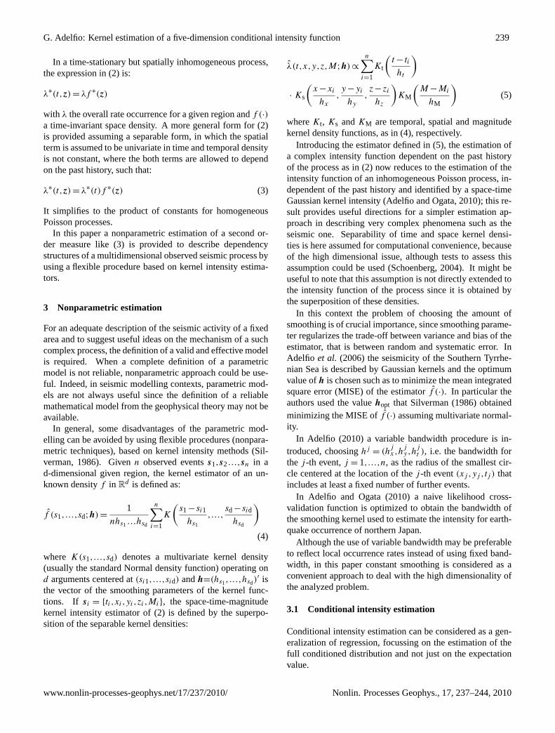
Fig. 1. 3-D space plot, with depth discretized into four groups withequispaced quantiles as breakpoints, so that all groups have roughlythe same number of points. Different colors are used for differentranges of magnitude: black for 4.5≤ M < 5.4, red for 5.4≤ M <

6.3 and green for 6.3≤ M < 7.2.

4 Application to New Zealand data and discussion

Space-time modelling seems one sensible direction, espe-cially if depth is also involved. Some pictures could suggestsomething about the evolution of spatial clusters at variousdepth (when they merge or separate). Deep earthquakes gen-erally lack fully evolved sequences which decay according tothe Omori’s lawUtsu(1961). Therefore clustering describedfrom ETAS model (Ogata, 1988) could be valid just for shal-lower events, that may have a classical aftershocks behavior.On the other hand, aftershocks for deep events have a differ-ent behavior and for this case a different modelling could beuseful, mostly to check their features that are still unknownin some sense.

Here a direct approach to analyze second order propertiesof deep earthquakes is considered, based on the use of thetwo point correlation function, that is of the conditional in-tensity function defined in (7).

We selected a subset of the GeoNet catalog of NewZealand earthquakes. Completeness issues of this catalogare discussed inHarte and Vere-Jones(1999). The data con-sist of n=3097 earthquakes oflocal magnitudeML=4.5 andlarger that are chosen from the wide region−43◦

∼ −37◦ Nand 171◦ ∼ 181◦ E and for the time span 1951∼ 2007. Thatarea is characterized by several deep events, with depth downto 530 km.

The bandwidth constants selected for the five-dimensionalintensity kernel estimator of the process arehx = 0.34,hy =

0.27,ht = 1000.86 (in days),hz = 0.06 andhM = 17.54.Some features of the observed events are now investigated.

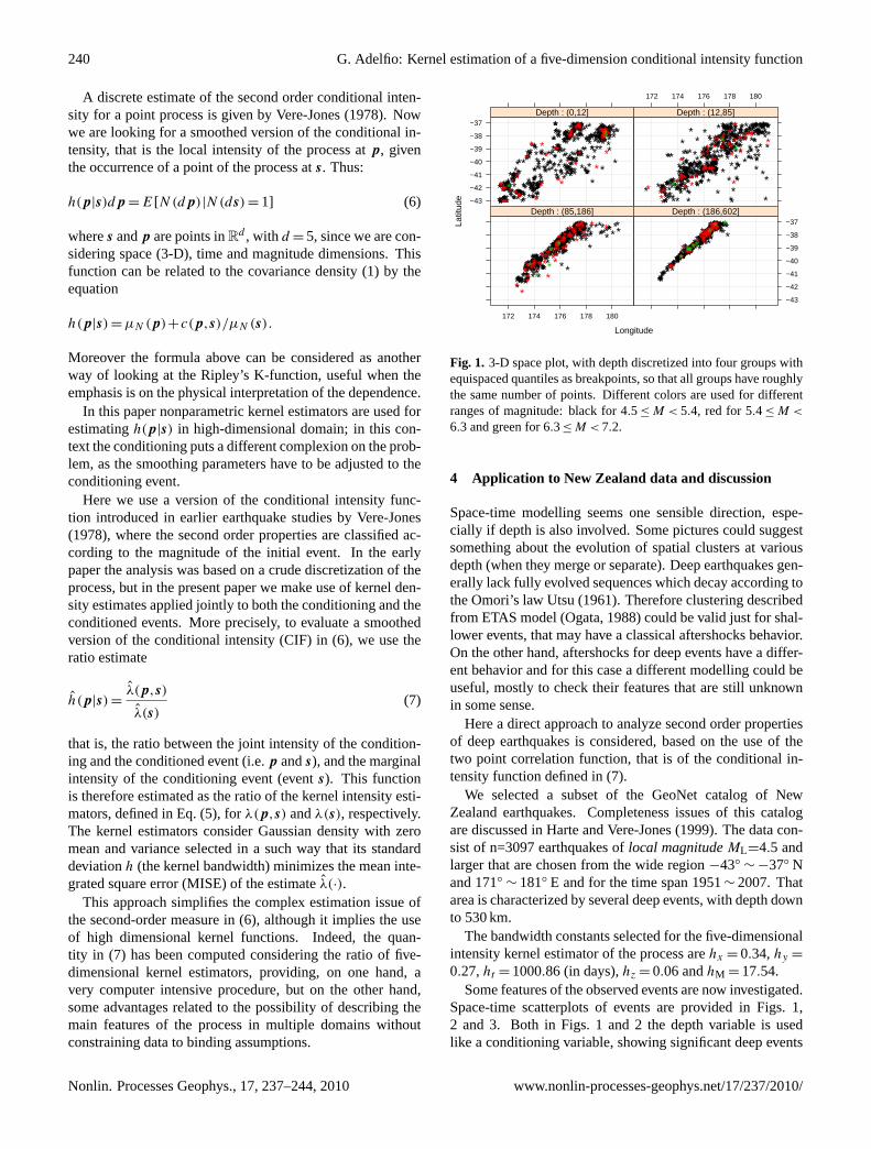
Space-time scatterplots of events are provided in Figs.1,2 and 3. Both in Figs.1 and 2 the depth variable is usedlike a conditioning variable, showing significant deep events



*****

**

**

*

**

** **

** *

*

* ** ***

*

*

***

*

**

*

*

**

**

****

*

*

**

****

***

*

*

*

**

*

*

*

**

**

**

*

*

*

*

***

*

*

**** **

*

*

*

*

*

*

*

***

**

*

*******

*

******************

*****

*

**

*

*******

*

***

*

***

*

**************

*

********

*

*

*

*****

*

****

*

******

*

**

*

*********

*

***************

**

****

*

**

*

*****

*

******

*

******************

*

****

* *

***

*

*********

*

********

*

**********************

*

****

*

********** **

*

**

*

*

*

*

******* ********

*

***

*

********

*

*

******

*

**

*

******* ***

*

* ****

*

** **

*

*****

*

****************

*

**** *

*

*

*

*

*

****

**

* **

*

*** ** *** ***** ** ** **

*

***

***

*

*

*

**

**

*

**

* ***

*

*******

*

****

*

***

***

*

*

*****

*

**

*

**

*

*

*

*

* *

**

*

*

*

**

*

**

*

*

*

*

* *

*

**

* *

**

*

*

*

*

*

*

**

*

**

** *

**

**

*

*

***

**

*

*

*

**

* ***

*

**

*

**

**

*

*

*

**

*

**

****

**

**

*

**

**

**

***

*

**

*

**

*

*

*

*

*

*

*

*

**

*

* *

*

**

****

*

*

**

**

*

**

*

** * **

**

***

*

*

*

**

*

*

***

*

*

*

*

*

**

*

*

***

**

*

*

*

**

**

**

****

*

**

*

* *

***

*

*

*

***

*

*

**

*

*********

*

*

*

*****************

**

******* **********************

****

*

*

**

*

*

**

*

**

** *

****

* *

***

***

*

***** *

**

**

*

**

*

***

*

*

*****

*

****

*

*

***

*

*****

**

*

** **

*

****

***

**

***

*

****

*

***

172

175178

181

−42

−40

−38−37

1951

1965

1979

1993

2007

LongitudeLatitude

Tim

e

: Depth (0,12]

*

*

* *** **

**

**

** *

**

**

*

*******

* *

*

**

*

**

*

* *

*

** *

*

*

*

**

**

*

*

*

*****

*

*

**

*

***

*****

*

*

**

*

*

***

*

*

*

**

**

**

***

*

*

**

*

*

*

*

***

**

*

*

**

**

***

**

**

** *

*

***

*

*

*

**

**

***

*

**

*

*

*

*

* *** *

*

*

*

**

*

*

*

****

*

**

**

*

***

*

*

*

****

**

*

*

*

*

* **

*

***

*

**

*

**

**

*

**

*

*

**

***

****

**

*

**

*

*** **

*

*

* **

***

**

*

*

*

*

*

*

**

* *** *

*

*

**

*

***

*

**

*

*****

**

**

***

*

*********

**

** *

*

*

*

*

*

*

** *

**

*

*

*

**

*

*

*

*

**

** *

*

* *

****

***

*

*

*

***

**

** *

*

*

*

*

*

*

*

*

*

*

*

*

*

*

**

*

*

*

**

*

*

*

*

*

***

***

*

**

*

**

*

*

*

*** ** **

**

*

*

**

*

*

**

**

*

*

*

***

*

*

*

*

*

*

*

**

*

*

***

**

**

*

* *

*

*

*

*

*

**

*

***

*

*

**

***

*

**

******* **

*

*****

* *

**

*

****

*

**

*

*

***

**

**

****

**

*

**

**

*

**

*

*

**

**

*

**

**

*

***

*

*

*

*

*

*

*

***

*

*

*

**

*

*

***

** *

*

**

**

*

**

*

***

*

**

*

*

**

*

**

*

****

*

*

*

*

**

**

*

*

*

**

*

**

*

*

*

**

* *

*

**

**

*

**

*

* *

*

******

*

*********

*

*** *

**** ***

**

*****

*

****

*

*

**

*

***

*

*

*

*

**

***

**

* **

***

*

***

**

*

**

**** ********

172

175178

181

−42

−40

−38−37

1951

1965

1979

1993

2007

LongitudeLatitude

Tim

e

: Depth (12,85]

*

*****

**

*** *

***

*

*

**

***

***

*

*

*

*

*****

*

*

** **

******

*

*

***

*

*

***

*

*

* * ***

***

***

***

*****

*

********

**

*

*

***

***

*** *

*

**

***

** ***

*

*

*

***

**

**

*

****

*

*

***

*

**

***

*

***

***

*

*

*

**

*

*

***

*

**

*

****

***

*******

*

****

*

******

*

*

*

****

*

*

**

*

**

********

*

**

**

*

*

****

*

***

**

*

*

**

***

*

*

*

**

*

***

*

*

**

**

**

**

*

*

*

***

*

*

*

**

***

**

*

***

*

**

**

**

*

**

*

*

***

*

*

****

**

*

*

*

*

*

*

*

*

**

*

*

***

**

*

*

*

*

*

*

******

*

***

*

**

**

**

**

***

*

****

*

*

*

*

****

** ****

**

*

**

*

*

*

**

*

*

*

*

***

*

***

*

*

*

***

**

*

*****

*

*****

***

****

**

*

*

**

*

****

*

**

*

**

*

*

**

*

******

*

*****

*

*

****

*

****

* *

**

**

*****************

*

*

*

*******

*

*

*

**

*

**

***

*

*

**

*

*******

*

**

**

*

*

*

*

*

****************

*

****

*

*

*

*

****

*

**

***

*

*

***

****

*

**

*

*

*

*

*

**

*

*

*

**

*****

****

*

***

*

***

*

**

*

*

*

**

*

*

**

*

**

*

*

*** *

*

*

*

*

*

*****

**

*

*

*

*

*

*

**

*

**

*

*

*

*

*

*

*

**

*

*

*

*

*

**

*

*

*

*

*

*

*

*

*

*

*

*

**

**

*

**

** *

**

***

**

* *

**

*

*

*

**

**

* ***

*

***

***

***

*

*

**

*

*

****

*

***

*

******

*

*******

******

*

**

****

*

**

**

*

**

*

**

**

*

*

*

*

*****

***

172

175178

181

−42

−40

−38−37

1951

1965

1979

1993

2007

LongitudeLatitude

Tim

e

: Depth (85,186]

*************

**

******

********

********

** ***

*

***

*********

*

******

***

*

*

*

**

*

*

*

*******

***

********

**

**

*****

****

****

******

*

*

****

*

*******

***

**********

************

********

*

*

*

**

***

***

*

*

*

******

***

*****

*

****

*

*

****

**

**

*

****

*

****

*

*

*

*

*

*

*

***

*

*

*******

*

*

****

**

*

**

*

**

*

*

****

*

********

*

**

***

***

*

*

*****

*

*

*

**

*

***

*

*

*

**

*

***

*

*

*

*

**

*

*

*****

***

**

*

*

*

*

*

****

**

***

*

***

**

*

**

*

*

*

*

*

**

**

*

*

*

*

********

*

*

*

*

****

*

***

***

****

*

**

**

*

*

***

*

****

*

*

***

***

*

*

*

*

*

*

**

*

******

*

*

**

*

*

**

**

****

*

****

*

***

*

***

**

*

*

**

*

*

*

**

**

***

*

*

*

*

*

*

***

*

***

*

*

***

**

*

*

**

*

**

*

****

*

**

*

***

*

*

*

*

**

*

*

***

*

**

*

**

*

*

*

*

*

****

*

**

*

*

****

**

*

*

***

*

**

****

*

*****

**

*

***

*

****

*

***

*

**

**

*

*

*

**

***

*

*

*

*

*

*

*

**

*

*

*****

****

*

*

*

*

***

***

**

*

*

****

*

**

*

*

*

*******

*

****

*

****

**

*

*

*****

**

**

******

*

*

***

*

********

**

*

*****

*

*******

**

*

*

*

*

***

*

**

***

****

**

*

***

*

*

**

*

*

*

*

*

*

*

***

*

*

*

*

*******

*

**

*

**

*

*******

*

**

*

*****

**

*

**

******

172

175178

181

−42

−40

−38−37

1951

1965

1979

1993

2007

LongitudeLatitude

Tim

e

: Depth (186,602]

Fig. 2. 3-D scatterplot of earthquakes epicenters in terms of latitude,longitude and time. Depth is used as the conditioning variable. Dif-ferent colors are used for different ranges of magnitude: black for4.5≤ M < 5.4, red for 5.4≤ M < 6.3 and green for 6.3≤ M < 7.2.

172

175178

181

−42

−40

−38−37

−601

−450

−300

−150

0

LongitudeLatitude

Dep

th

: Magnitude (4.5,5.17]

172

175178

181

−42

−40

−38−37

−601

−450

−300

−150

0

LongitudeLatitude

Dep

th

: Magnitude (5.17,5.85]

172

175178

181

−42

−40

−38−37

−601

−450

−300

−150

0

LongitudeLatitude

Dep

th

: Magnitude (5.85,6.53]

172

175178

181

−42

−40

−38−37

−601

−450

−300

−150

0

LongitudeLatitude

Dep

th

: Magnitude (6.53,7.2]

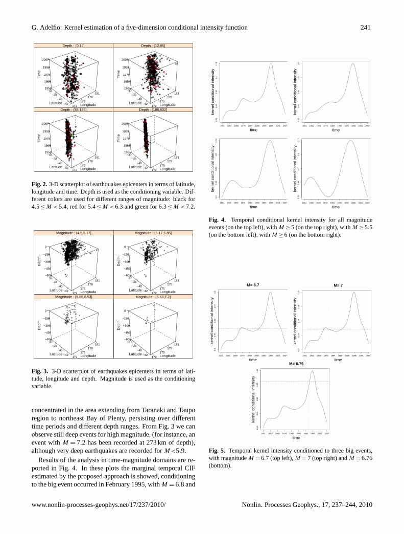
Fig. 3. 3-D scatterplot of earthquakes epicenters in terms of lati-tude, longitude and depth. Magnitude is used as the conditioningvariable.

concentrated in the area extending from Taranaki and Tauporegion to northeast Bay of Plenty, persisting over differenttime periods and different depth ranges. From Fig.3 we canobserve still deep events for high magnitude, (for instance, anevent withM = 7.2 has been recorded at 273 km of depth),although very deep earthquakes are recorded forM<5.9.

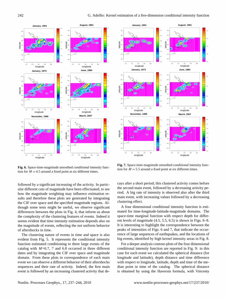
Results of the analysis in time-magnitude domains are re-ported in Fig.4. In these plots the marginal temporal CIFestimated by the proposed approach is showed, conditioningto the big event occurred in February 1995, withM = 6.8 and

time

kern

el c

ondi

tiona

l int

ensi

ty

1951 1962 1969 1976 1984 1990 1995 1996 2001 2007

0.25

0.63

1.02

1.4

1.79

time

kern

el c

ondi

tiona

l int

ensi

ty

1951 1962 1969 1976 1984 1990 1995 1996 2001 2007

0.32

0.62

0.92

1.22

1.52

time

kern

el c

ondi

tiona

l int

ensi

ty

1951 1962 1969 1976 1984 1990 1995 1996 2001 2007

0.3

0.56

0.81

1.07

1.32

time

kern

el c

ondi

tiona

l int

ensi

ty

1951 1962 1969 1976 1984 1990 1995 1996 2001 2007

0.28

0.49

0.7

0.9

1.11

Fig. 4. Temporal conditional kernel intensity for all magnitudeevents (on the top left), withM ≥ 5 (on the top right), withM ≥ 5.5(on the bottom left), withM ≥ 6 (on the bottom right).

M= 6.7

time

kern

el c

ondi

tiona

l int

ensi

ty

1951 1962 1969 1976 1984 1990 1995 1996 2001 2007

0.3

0.78

1.25

1.73

2.2

M= 7

time

kern

el c

ondi

tiona

l int

ensi

ty

1951 1962 1969 1976 1984 1990 1995 1996 2001 2007

0.31

0.79

1.28

1.76

2.25

M= 6.76

time

kern

el c

ondi

tiona

l int

ensi

ty

1951 1962 1969 1976 1984 1990 1995 1996 2001 2007

0.16

0.42

0.68

0.93

1.19

Fig. 5. Temporal kernel intensity conditioned to three big events,with magnitudeM = 6.7 (top left),M = 7 (top right) andM = 6.76(bottom).



0.0

0.5

1.0

1.5

2.0

2.5

172 174 176 178 180

−46

−44

−42

−40

−38

−36

−34

January, 1951

longitude

latit

ude

0

2

4

6

8

172 174 176 178 180

−46

−44

−42

−40

−38

−36

−34

August, 1961

longitudela

titud

e

0

2

4

6

8

10

12

172 174 176 178 180

−46

−44

−42

−40

−38

−36

−34

January, 1973

longitude

latit

ude

0

1

2

3

4

5

6

172 174 176 178 180

−46

−44

−42

−40

−38

−36

−34

June, 1984

longitude

latit

ude

0

10

20

30

40

172 174 176 178 180

−46

−44

−42

−40

−38

−36

−34

November, 1995

longitude

latit

ude

0

1

2

3

4

5

6

172 174 176 178 180

−46

−44

−42

−40

−38

−36

−34

March, 2007

longitude

latit

ude

Fig. 6. Space-time-magnitude smoothedconditionalintensity func-tion for M = 4.5 around a fixed point at six different times.

followed by a significant increasing of the activity. In partic-ular different cuts of magnitude have been effectuated, to seehow the magnitude weighting may influence estimation re-sults and therefore these plots are generated by integratingthe CIF over space and the specified magnitude regions. Al-though some tests might be useful, we observe significantdifferences between the plots in Fig.4, that inform us aboutthe complexity of the clustering features of events. Indeed itseems evident that time intensity estimation depends also onthe magnitude of events, reflecting the not uniform behaviorof aftershocks in time.

The clustering nature of events in time and space is alsoevident from Fig.5. It represents the conditional intensityfunction estimated conditioning to three large events of thecatalog withM=6.7, 7 and 6.8 occurred in three differentdates and by integrating the CIF over space and magnitudedomain. From these plots in correspondence of each mainevent we can observe a different behavior of their aftershockssequences and their rate of activity. Indeed, the first mainevent is followed by an increasing clustered activity that de-

0.0

0.2

0.4

0.6

0.8

1.0

1.2

172 174 176 178 180

−46

−44

−42

−40

−38

−36

−34

January, 1951

longitude

latit

ude

0.0

0.5

1.0

1.5

2.0

172 174 176 178 180

−46

−44

−42

−40

−38

−36

−34

August, 1961

longitude

latit

ude

0.0

0.2

0.4

0.6

0.8

1.0

1.2

172 174 176 178 180

−46

−44

−42

−40

−38

−36

−34

January, 1973

longitude

latit

ude

0.0

0.5

1.0

1.5

172 174 176 178 180

−46

−44

−42

−40

−38

−36

−34

June, 1984

longitude

latit

ude

0

2

4

6

8

10

172 174 176 178 180

−46

−44

−42

−40

−38

−36

−34

November, 1995

longitude

latit

ude

0.0

0.5

1.0

1.5

2.0

2.5

3.0

3.5

172 174 176 178 180

−46

−44

−42

−40

−38

−36

−34

March, 2007

longitude

latit

ude


cays after a short period; this clustered activity comes beforethe second main event, followed by a decreasing activity pe-riod. A big rate of intensity is observed also after the thirdmain event, with increasing values followed by a decreasingclustering effect.

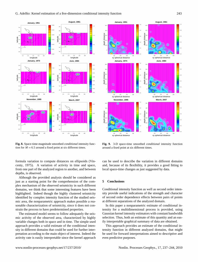
A four dimensional conditional intensity function is esti-mated for time-longitude-latitude-magnitude domains. Thespace-time marginal function with respect depth for differ-ent levels of magnitude (4.5, 5.5, 6.5) is shown in Figs.6–8.It is interesting to highlight the correspondence between thepeaks of intensities of Figs.6 and7, that indicate the occur-rence of large sequences of earthquakes, and the locations ofbig events, identified by high kernel intensity areas in Fig.8.

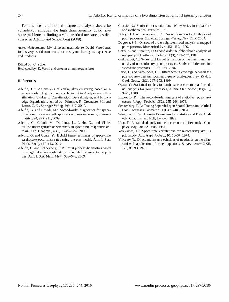
For a deeper analysis contour-plots of the four dimensionalconditional intensity function are reported in Fig.9: in thiscase for each event we calculated the spherical distance (forlongitude and latitude), depth distance and time differencewith respect to longitude, latitude, depth and time of the me-dian point in time of the catalog. The spherical distanceis obtained by using the Haversin formula, with Vincenty



0.000

0.001

0.002

0.003

0.004

0.005

0.006

172 174 176 178 180

−46

−44

−42

−40

−38

−36

−34

January, 1951

longitude

latit

ude

0.0

0.5

1.0

1.5

172 174 176 178 180

−46

−44

−42

−40

−38

−36

−34

August, 1961

longitudela

titud

e

0.00

0.01

0.02

0.03

0.04

172 174 176 178 180

−46

−44

−42

−40

−38

−36

−34

January, 1973

longitude

latit

ude

0.00

0.02

0.04

0.06

0.08

0.10

0.12

0.14

172 174 176 178 180

−46

−44

−42

−40

−38

−36

−34

June, 1984

longitude

latit

ude

0.0

0.2

0.4

0.6

0.8

1.0

172 174 176 178 180

−46

−44

−42

−40

−38

−36

−34

November, 1995

longitude

latit

ude

0.00

0.05

0.10

0.15

172 174 176 178 180

−46

−44

−42

−40

−38

−36

−34

March, 2007

longitude

latit

ude


formula variation to compute distances on ellipsoids (Vin-centy, 1975). A variation of activity in time and space,from one part of the analyzed region to another, and betweendepths, is observed.

Although the provided analysis should be considered asjust as a starting point for the comprehension of the com-plex mechanism of the observed seismicity in such differentdomains, we think that some interesting features have beenhighlighted. Indeed though the highly clustered seismicityidentified by complex intensity function of the studied seis-mic area, the nonparametric approach makes possible a rea-sonable characterization of seismicity, since it does not con-strain the process to have predetermined properties.

The estimated model seems to follow adequately the seis-mic activity of the observed area, characterized by highlyvariable changes both in space and in time. The simple usedapproach provides a valid estimate of the conditional inten-sity in different domains that could be used for further inter-pretation according to the main object of interest. Indeed theactivity rate is easily interpretable since the kernel approach

0.0

0.2

0.4

0.6

0.8

1.0

200 400 600 800

0

100

200

300

400

500

January, 1951

xy spherical distance

dept

h di

stan

ce

0.0

0.2

0.4

0.6

0.8

1.0

200 400 600 800

0

100

200

300

400

500

August, 1961


dept

h di

stan

ce

0.0

0.2

0.4

0.6

0.8

1.0

200 400 600 800

0

100

200

300

400

500

January, 1973


dept

h di

stan

ce

0.0

0.2

0.4

0.6

0.8

1.0

200 400 600 800

0

100

200

300

400

500

June, 1984


dept

h di

stan

ce

0.0

0.2

0.4

0.6

0.8

1.0

200 400 600 800

0

100

200

300

400

500

November, 1995


dept

h di

stan

ce

0.0

0.2

0.4

0.6

0.8

1.0

200 400 600 800

0

100

200

300

400

500

March, 2007


dept

h di

stan

ceFig. 9. 3-D space-time smoothedconditional intensity functionaround a fixed point at six different times.

can be used to describe the variation in different domainsand, because of its flexibility, it provides a good fitting tolocal space-time changes as just suggested by data.

5 Conclusions

Conditional intensity function as well as second order inten-sity provide useful indications of the strength and characterof second order dependence effects between pairs of pointsat different separations of the analyzed domain.

In this paper a nonparametric estimate of conditional in-tensity for a multidimensional process is provided, usingGaussian kernel intensity estimators with constant bandwidthselection. Thus, both an estimate of this quantity and an eas-ily interpretable graphical summary of data are obtained.

This approach provides an estimate of the conditional in-tensity function in different analyzed domains, that mightbe used for forward interpretations aimed to descriptive andeven predictive purposes.



For this reason, additional diagnostic analysis should beconsidered, although the high dimensionality could givesome problems in finding a valid residual measures, as dis-cussed inAdelfio and Schoenberg(2009).

Acknowledgements.My sincerest gratitude to David Vere-Jonesfor his very useful comments, but mostly for sharing his experienceand kindness.

Edited by: G. ZollerReviewed by: E. Varini and another anonymous referee

References

Adelfio, G.: An analysis of earthquakes clustering based on asecond-order diagnostic approach, in: Data Analysis and Clas-sification, Studies in Classification, Data Analysis, and Knowl-edge Organization, edited by: Palumbo, F., Greenacre, M., andLauro, C. N., Springer-Verlag, 309–317, 2010.

Adelfio, G. and Chiodi, M.: Second-order diagnostics for space-time point processes with application to seismic events, Environ-metrics, 20, 895–911, 2009.

Adelfio, G., Chiodi, M., De Luca, L., Luzio, D., and Vitale,M.: Southern-tyrrhenian seismicity in space-time-magnitude do-main, Ann. Geophys., 49(6), 1245–1257, 2006.

Adelfio, G. and Ogata, Y.: Hybrid kernel estimates of space-timeearthquake occurrance rates using the etas model, Ann. I. Stat.Math., 62(1), 127–143, 2010.

Adelfio, G. and Schoenberg, F. P.: Point process diagnostics basedon weighted second-order statistics and their asymptotic proper-ties, Ann. I. Stat. Math, 61(4), 929–948, 2009.

Cressie, N.: Statistics for spatial data, Wiley series in probabilityand mathematical statistics, 1991.

Daley, D. J. and Vere-Jones, D.: An introduction to the theory ofpoint processes, 2nd edn., Springer-Verlag, New York, 2003.

Doguwa, S. I.: On second order neighbourhood analysis of mappedpoint patterns. Biometrical J., 4, 451–457, 1989.

Getis, A. and Franklin, J.: Second order neighbourhood analysis ofmapped point patterns, Ecology, 68(3), 473–477, 1987.

Grillenzoni, C.: Sequenzial kernel estimation of the conditional in-tensity of nonstationary point processes, Statistical inference forstochastic processes, 9, 135–160, 2006.

Harte, D. and Vere-Jones, D.: Differences in coverage between thepde and new zealand local earthquake catalogues, New Zeal. J.Geol. Geop., 42(2), 237–253, 1999.

Ogata, Y.: Statistical models for earthquake occurrences and resid-ual analysis for point processes, J. Am. Stat. Assoc., 83(401),9–27, 1988.

Ripley, B. D.: The second-order analysis of stationary point pro-cesses, J. Appl. Probab., 13(2), 255–266, 1976.

Schoenberg, F. P.: Testing Separability in Spatial-Temporal MarkedPoint Processes, Biometrics, 60, 471–481, 2004.

Silverman, B. W.: Density Estimation for Statistics and Data Anal-ysis, Chapman and Hall, London, 1986.

Utsu, T.: A statistical study on the occurrence of aftershocks, Geo-phys. Mag., 30, 521–605, 1961.

Vere-Jones, D.: Space-time correlations for microearthquakes: apilot study, Adv. Appl. Probab., 10, 73–87, 1978.

Vincenty, T.: Direct and inverse solutions of geodesics on the ellip-soid with application of nested equations, Survey review XXII,176, 89–93, 1975.


Documents

Kernel estimation and display of a five-dimensional … estimation and display of a five-dimensional conditional intensity function G. Adelfio Dipartimento di Scienze Statistiche