Kinematics of Robots - Idaho State Universityperealba/courses/KinematicsNotes/Chapter1.pdf · 2 Robot Kinematics Using Matrix Algebra 25 ... 8.7 Planar motion and planar geometry:

Kinematics of Robots

Alba Perez Gracia

c© Draft date September 9, 2011

Contents

Contents i

1 Motion: An Introduction 3

1.1 Overview . . . . . . . . . . . . . . . . . . . . . . . . . . . . . . . . . . . . . . . . . . 3

1.2 Introduction . . . . . . . . . . . . . . . . . . . . . . . . . . . . . . . . . . . . . . . . . 3

1.3 The finite displacement . . . . . . . . . . . . . . . . . . . . . . . . . . . . . . . . . . 4

1.3.1 Translations . . . . . . . . . . . . . . . . . . . . . . . . . . . . . . . . . . . . . 5

1.3.2 Rotations . . . . . . . . . . . . . . . . . . . . . . . . . . . . . . . . . . . . . . 6

1.3.3 General finite displacements . . . . . . . . . . . . . . . . . . . . . . . . . . . . 10

1.3.4 The invariants of a general displacement . . . . . . . . . . . . . . . . . . . . . 11

1.4 A little bit of line geometry . . . . . . . . . . . . . . . . . . . . . . . . . . . . . . . . 12

1.4.1 Dual vector algebra . . . . . . . . . . . . . . . . . . . . . . . . . . . . . . . . 13

1.4.2 More line geometry . . . . . . . . . . . . . . . . . . . . . . . . . . . . . . . . . 15

1.4.3 Line motion . . . . . . . . . . . . . . . . . . . . . . . . . . . . . . . . . . . . . 15

1.4.4 Line Geometry and the Klein Quadric . . . . . . . . . . . . . . . . . . . . . . 16

1.5 The screw axis of a general displacement and Chasles’ Theorem . . . . . . . . . . . . 16

1.6 More on Matrix Representation . . . . . . . . . . . . . . . . . . . . . . . . . . . . . . 19

1.6.1 How to create a rotation matrix . . . . . . . . . . . . . . . . . . . . . . . . . 19

1.6.2 Homogeneous matrix representation . . . . . . . . . . . . . . . . . . . . . . . 21

i

ii CONTENTS

2 Robot Kinematics Using Matrix Algebra 25

2.1 Overview . . . . . . . . . . . . . . . . . . . . . . . . . . . . . . . . . . . . . . . . . . 25

2.2 Robot Kinematics . . . . . . . . . . . . . . . . . . . . . . . . . . . . . . . . . . . . . 25

2.3 Basic joints . . . . . . . . . . . . . . . . . . . . . . . . . . . . . . . . . . . . . . . . . 27

2.4 Forward Kinematics Equations . . . . . . . . . . . . . . . . . . . . . . . . . . . . . . 28

2.4.1 Denavit-Hartenberg parameters . . . . . . . . . . . . . . . . . . . . . . . . . . 28

2.4.2 Kinematics Equations . . . . . . . . . . . . . . . . . . . . . . . . . . . . . . . 30

2.5 Forward Kinematics Example . . . . . . . . . . . . . . . . . . . . . . . . . . . . . . . 31

2.6 Inverse Kinematics . . . . . . . . . . . . . . . . . . . . . . . . . . . . . . . . . . . . . 32

2.7 Inverse Kinematics Example . . . . . . . . . . . . . . . . . . . . . . . . . . . . . . . . 33

3 Group Theory and Motion 35

3.1 Overview . . . . . . . . . . . . . . . . . . . . . . . . . . . . . . . . . . . . . . . . . . 35

3.2 Group Theory Review . . . . . . . . . . . . . . . . . . . . . . . . . . . . . . . . . . . 35

3.2.1 Subgroups . . . . . . . . . . . . . . . . . . . . . . . . . . . . . . . . . . . . . . 36

3.2.2 Automorphisms . . . . . . . . . . . . . . . . . . . . . . . . . . . . . . . . . . . 37

3.2.3 Products of Groups . . . . . . . . . . . . . . . . . . . . . . . . . . . . . . . . 38

3.2.4 Cosets and Actions . . . . . . . . . . . . . . . . . . . . . . . . . . . . . . . . . 39

3.3 The group of finite displacements . . . . . . . . . . . . . . . . . . . . . . . . . . . . . 40

3.3.1 Subgroups of the Special Euclidean Group . . . . . . . . . . . . . . . . . . . . 41

4 Lie Groups and Lie Algebras 43

4.1 Introduction . . . . . . . . . . . . . . . . . . . . . . . . . . . . . . . . . . . . . . . . . 43

4.2 Lie groups . . . . . . . . . . . . . . . . . . . . . . . . . . . . . . . . . . . . . . . . . . 43

4.3 One-parameter subgroups . . . . . . . . . . . . . . . . . . . . . . . . . . . . . . . . . 44

4.4 The Lie Algebra . . . . . . . . . . . . . . . . . . . . . . . . . . . . . . . . . . . . . . 45

4.4.1 The Lie bracket . . . . . . . . . . . . . . . . . . . . . . . . . . . . . . . . . . . 46

CONTENTS iii

4.4.2 Chasles’ Theorem again . . . . . . . . . . . . . . . . . . . . . . . . . . . . . . 48

4.5 The Lie algebra of the Special Euclidean Group SE(3) . . . . . . . . . . . . . . . . . 48

4.5.1 Relative Rotations . . . . . . . . . . . . . . . . . . . . . . . . . . . . . . . . . 48

4.5.2 Relative general motion . . . . . . . . . . . . . . . . . . . . . . . . . . . . . . 49

4.5.3 Rigid body velocity . . . . . . . . . . . . . . . . . . . . . . . . . . . . . . . . 50

4.6 Example . . . . . . . . . . . . . . . . . . . . . . . . . . . . . . . . . . . . . . . . . . . 51

5 The Product of Exponentials for Serial Manipulators 53

5.1 Introduction . . . . . . . . . . . . . . . . . . . . . . . . . . . . . . . . . . . . . . . . . 53

5.2 Forward Kinematics . . . . . . . . . . . . . . . . . . . . . . . . . . . . . . . . . . . . 53

5.3 Example: Epson E2L Scara Robot . . . . . . . . . . . . . . . . . . . . . . . . . . . . 54

5.4 Velocity and Jacobian . . . . . . . . . . . . . . . . . . . . . . . . . . . . . . . . . . . 56

5.4.1 Example . . . . . . . . . . . . . . . . . . . . . . . . . . . . . . . . . . . . . . . 57

5.5 Inverse and pseudoinverse Jacobian . . . . . . . . . . . . . . . . . . . . . . . . . . . . 58

6 Grassmann Algebra 59

6.1 Overview . . . . . . . . . . . . . . . . . . . . . . . . . . . . . . . . . . . . . . . . . . 59

6.2 Vector spaces and metric spaces . . . . . . . . . . . . . . . . . . . . . . . . . . . . . . 59

6.3 Algebras . . . . . . . . . . . . . . . . . . . . . . . . . . . . . . . . . . . . . . . . . . . 61

6.4 Grassmann Algebra . . . . . . . . . . . . . . . . . . . . . . . . . . . . . . . . . . . . 61

6.4.1 Grassmann algebra associated to R3 . . . . . . . . . . . . . . . . . . . . . . . 62



6.4.4 The general Grassman algebra . . . . . . . . . . . . . . . . . . . . . . . . . . 66

6.5 More on Grassmann algebra . . . . . . . . . . . . . . . . . . . . . . . . . . . . . . . . 68

7 Quaternions 71

7.1 Overview . . . . . . . . . . . . . . . . . . . . . . . . . . . . . . . . . . . . . . . . . . 71

iv CONTENTS

7.2 Quaternions . . . . . . . . . . . . . . . . . . . . . . . . . . . . . . . . . . . . . . . . . 71

7.3 Unit Quaternions and Rotations . . . . . . . . . . . . . . . . . . . . . . . . . . . . . 73

7.3.1 Rotation by a unit quaternion . . . . . . . . . . . . . . . . . . . . . . . . . . . 73

7.4 The Lie Algebra of Unit Quaternions . . . . . . . . . . . . . . . . . . . . . . . . . . . 75

7.4.1 Euler parameters revisited . . . . . . . . . . . . . . . . . . . . . . . . . . . . . 76

7.5 Applications . . . . . . . . . . . . . . . . . . . . . . . . . . . . . . . . . . . . . . . . . 76

7.5.1 Satellite navigation . . . . . . . . . . . . . . . . . . . . . . . . . . . . . . . . . 76

7.5.2 Singularities in the Euler angles matrix representation . . . . . . . . . . . . . 78

7.5.3 Trajectory planning and interpolation . . . . . . . . . . . . . . . . . . . . . . 79

8 Clifford Algebras 81

8.1 Overview . . . . . . . . . . . . . . . . . . . . . . . . . . . . . . . . . . . . . . . . . . 81

8.2 Clifford algebras and the Clifford product . . . . . . . . . . . . . . . . . . . . . . . . 82

8.2.1 Properties of the geometric product . . . . . . . . . . . . . . . . . . . . . . . 83

8.3 Creating Clifford algebras . . . . . . . . . . . . . . . . . . . . . . . . . . . . . . . . . 83

8.3.1 More on the geometric product . . . . . . . . . . . . . . . . . . . . . . . . . . 84

8.4 Subalgebras . . . . . . . . . . . . . . . . . . . . . . . . . . . . . . . . . . . . . . . . . 85

8.5 Duality . . . . . . . . . . . . . . . . . . . . . . . . . . . . . . . . . . . . . . . . . . . 86

8.6 Actions . . . . . . . . . . . . . . . . . . . . . . . . . . . . . . . . . . . . . . . . . . . 86

8.6.1 Mappings . . . . . . . . . . . . . . . . . . . . . . . . . . . . . . . . . . . . . . 87

8.6.2 The action by ”Clifford conjugation” . . . . . . . . . . . . . . . . . . . . . . . 88

8.7 Planar motion and planar geometry: Clifford algebras . . . . . . . . . . . . . . . . . 89

8.7.1 Clifford algebra of the Euclidean plane: C2,0,0 . . . . . . . . . . . . . . . . . . 89

8.8 The Clifford algebra of the three-dimensional space R3 . . . . . . . . . . . . . . . . . 90

8.8.1 The even Clifford algebra of the three-dimensional space R3 . . . . . . . . . . 91

8.9 The even Clifford algebra of the projective space P3 . . . . . . . . . . . . . . . . . . 91

8.10 Equivalent algebras . . . . . . . . . . . . . . . . . . . . . . . . . . . . . . . . . . . . . 93

CONTENTS v

8.11 The Clifford algebra of dual quaternions . . . . . . . . . . . . . . . . . . . . . . . . . 95

8.11.1 Spatial displacements using unit dual quaternions . . . . . . . . . . . . . . . 96

8.11.2 Examples . . . . . . . . . . . . . . . . . . . . . . . . . . . . . . . . . . . . . . 99

8.12 The geometry of the Clifford algebra C+(P3, d) . . . . . . . . . . . . . . . . . . . . . 99

8.13 Planar, spherical and spatial displacements . . . . . . . . . . . . . . . . . . . . . . . 103

8.13.1 Planar displacements . . . . . . . . . . . . . . . . . . . . . . . . . . . . . . . . 103

8.13.2 Spherical motion . . . . . . . . . . . . . . . . . . . . . . . . . . . . . . . . . . 104

8.13.3 Isomorphisms . . . . . . . . . . . . . . . . . . . . . . . . . . . . . . . . . . . . 104

8.14 Lie algebra and Clifford algebra . . . . . . . . . . . . . . . . . . . . . . . . . . . . . . 106

8.15 Clifford Analysis . . . . . . . . . . . . . . . . . . . . . . . . . . . . . . . . . . . . . . 107

9 Robot Kinematics Using Clifford Algebras 111

9.1 Screw displacement about a joint . . . . . . . . . . . . . . . . . . . . . . . . . . . . . 111

9.2 Robot kinematics equations . . . . . . . . . . . . . . . . . . . . . . . . . . . . . . . . 113

9.2.1 Forward kinematics . . . . . . . . . . . . . . . . . . . . . . . . . . . . . . . . 113

9.2.2 Inverse kinematics . . . . . . . . . . . . . . . . . . . . . . . . . . . . . . . . . 114

9.2.3 Example: Epson E2L Scara Robot . . . . . . . . . . . . . . . . . . . . . . . . 114

9.3 Differential kinematics and Jacobian . . . . . . . . . . . . . . . . . . . . . . . . . . . 116

9.3.1 Example: Epson E2L Scara Robot . . . . . . . . . . . . . . . . . . . . . . . . 118

9.4 Kinematic Synthesis . . . . . . . . . . . . . . . . . . . . . . . . . . . . . . . . . . . . 119

9.4.1 Overview . . . . . . . . . . . . . . . . . . . . . . . . . . . . . . . . . . . . . . 119

9.4.2 4R Synthesis . . . . . . . . . . . . . . . . . . . . . . . . . . . . . . . . . . . . 119

Bibliography 73

vi CONTENTS

List of Figures

1.1 Description of the motion of a rigid body . . . . . . . . . . . . . . . . . . . . . . . . 4

1.2 (a) A pure translation and (b) a pure rotation of a rigid body . . . . . . . . . . . . . 5

1.3 A rigid displacement . . . . . . . . . . . . . . . . . . . . . . . . . . . . . . . . . . . . 6

1.4 Composition of displacements . . . . . . . . . . . . . . . . . . . . . . . . . . . . . . . 11

1.5 A relative displacement . . . . . . . . . . . . . . . . . . . . . . . . . . . . . . . . . . 12

1.6 A line defined using Plucker coordinates . . . . . . . . . . . . . . . . . . . . . . . . . 13

1.7 Dual vector geometry . . . . . . . . . . . . . . . . . . . . . . . . . . . . . . . . . . . 14

1.8 The screw axis, rotation angle and slide of a displacement . . . . . . . . . . . . . . . 18

1.9 Euler angles . . . . . . . . . . . . . . . . . . . . . . . . . . . . . . . . . . . . . . . . . 20

2.1 Reachable workspace, Adept Viper m650 robot (Adept Technologies, Inc.) . . . . . . 27

2.2 Common types of joints . . . . . . . . . . . . . . . . . . . . . . . . . . . . . . . . . . 28

2.3 Local transformations along the links of a robot. . . . . . . . . . . . . . . . . . . . . 29

2.4 Example: a three-jointed serial robot. . . . . . . . . . . . . . . . . . . . . . . . . . . 31

2.5 Welding Robot (Fanuc Robotics) . . . . . . . . . . . . . . . . . . . . . . . . . . . . . 34

2.5 Welding Robot (Fanuc Robotics) . . . . . . . . . . . . . . . . . . . . . . . . . . . . . 32

5.1 SCARA robot Epson E2L65 . . . . . . . . . . . . . . . . . . . . . . . . . . . . . . . . 54

6.1 H.G. Grassmann . . . . . . . . . . . . . . . . . . . . . . . . . . . . . . . . . . . . . . 62

6.2 The wedge product of two vectors . . . . . . . . . . . . . . . . . . . . . . . . . . . . 64

vii

viii LIST OF FIGURES

7.1 Sir W.R. Hamilton . . . . . . . . . . . . . . . . . . . . . . . . . . . . . . . . . . . . . 72

7.2 ECI coordinates . . . . . . . . . . . . . . . . . . . . . . . . . . . . . . . . . . . . . . . 78

7.3 A spherical wrist . . . . . . . . . . . . . . . . . . . . . . . . . . . . . . . . . . . . . . 79

7.4 The Agile Eye . . . . . . . . . . . . . . . . . . . . . . . . . . . . . . . . . . . . . . . . 80

8.1 W. H. Clifford . . . . . . . . . . . . . . . . . . . . . . . . . . . . . . . . . . . . . . . . 82

8.2 Planar, spherical and spatial displacements . . . . . . . . . . . . . . . . . . . . . . . 104

9.1 SCARA robot Epson E2L65 . . . . . . . . . . . . . . . . . . . . . . . . . . . . . . . . 115

List of Tables

2.1 Denavit-Hartenberg parameters. . . . . . . . . . . . . . . . . . . . . . . . . . . . . . 30

2.2 Denavit-Hartenberg parameters for the robot of Figure 2.4. . . . . . . . . . . . . . . 31

3.1 Subgroups of the group of spatial displacements . . . . . . . . . . . . . . . . . . . . . 41

6.1 Basis multivectors for the Grassman algebra of R3 . . . . . . . . . . . . . . . . . . . 65

6.2 Basis multivectors for the Grassman algebra of R4 . . . . . . . . . . . . . . . . . . . 66

6.3 Basis multivectors for the Grassman algebra of Rm . . . . . . . . . . . . . . . . . . . 67

8.1 Multiplication table for C2,0,0 . . . . . . . . . . . . . . . . . . . . . . . . . . . . . . . 89

8.2 Multiplication table for C+3,0,1 . . . . . . . . . . . . . . . . . . . . . . . . . . . . . . . 94


8.4 Another multiplication table for C+0,3,1 . . . . . . . . . . . . . . . . . . . . . . . . . . 95

8.5 Matrix and Clifford algebra expressions for rotations and general displacements. . . 96



1

2 LIST OF TABLES

Chapter 1

Motion: An Introduction

1.1 Overview

This notes are designed as a gentle introduction to the use of Clifford algebras in robot kinematics.

In the process, other key concepts will be reviewed, concepts that Clifford algebras build upon.

Basic group theory, linear spaces, Grassman spaces and Lie algebras, as well as line geometry and

projective geometry, will be introduced. Each of these topics is accompanied by examples and

applications of increasing difficulty.

1.2 Introduction

Kinematics is defined as the study of the motion, regardless of the forces causing it and caused by

it. Motion is a concept that includes position and its derivatives, mainly velocity and acceleration.

The subjects that we study are modeled as rigid bodies. A rigid body is a set of particles such

that the distance between them remains fixed. This means that, unlike individual particles, we can

define not only location, velocity and acceleration of a particle in the body, but also orientation,

angular velocity and angular acceleration of the body. Orientation is defined as a shortcut to avoid

describing the motion of a set of particles in the body; for completely defining the position of a

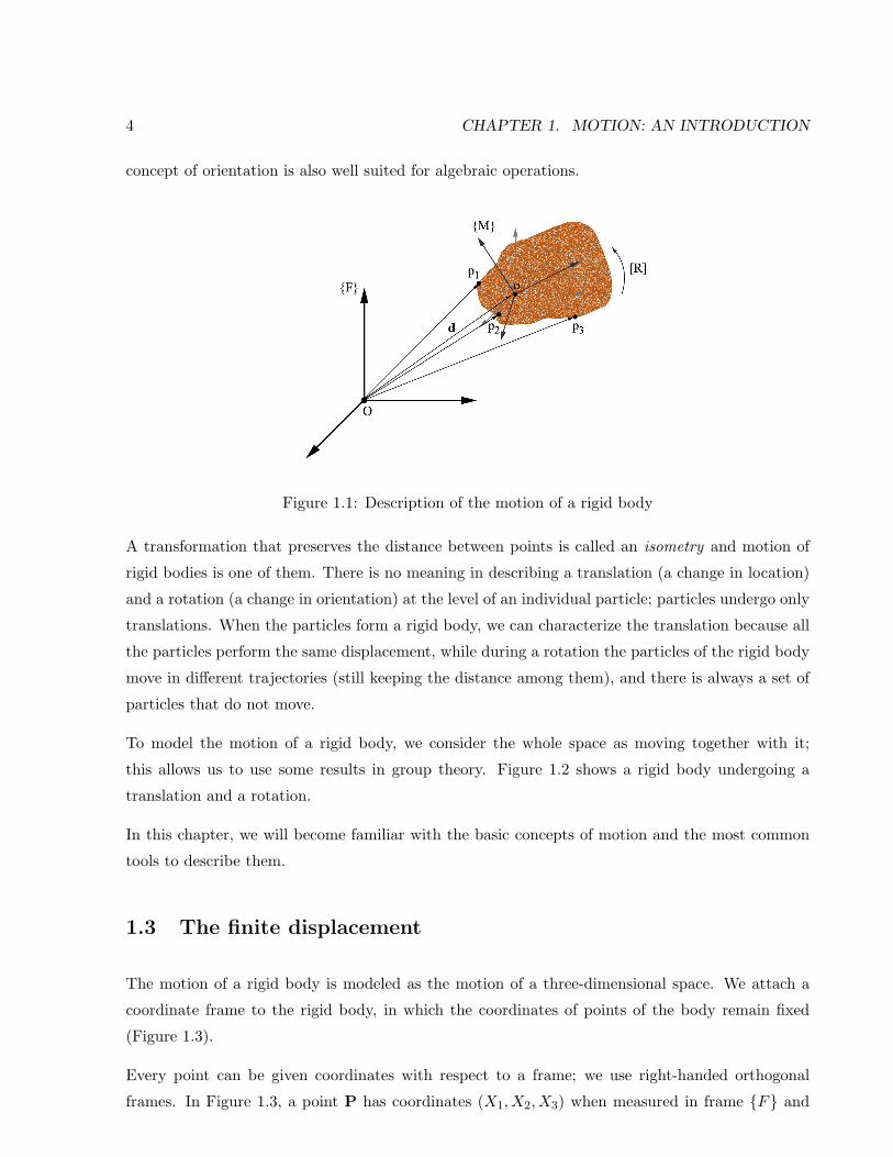
rigid body, we need to define the location of at least three particles on it, p1, p2 and p3, that is 9

parameters. However, the three locations are not independent, because the distance between each

two particles must remain constant; this adds three constraints to the set of nine parameters. Or

we can define the location of one particle and the orientation of a frame attached to the body at

that point, in which case we just need to define six parameters, given by d and [R] in Fig 1.1. The

3

4 CHAPTER 1. MOTION: AN INTRODUCTION

concept of orientation is also well suited for algebraic operations.

Figure 1.1: Description of the motion of a rigid body

A transformation that preserves the distance between points is called an isometry and motion of

rigid bodies is one of them. There is no meaning in describing a translation (a change in location)

and a rotation (a change in orientation) at the level of an individual particle; particles undergo only

translations. When the particles form a rigid body, we can characterize the translation because all

the particles perform the same displacement, while during a rotation the particles of the rigid body

move in different trajectories (still keeping the distance among them), and there is always a set of

particles that do not move.

To model the motion of a rigid body, we consider the whole space as moving together with it;

this allows us to use some results in group theory. Figure 1.2 shows a rigid body undergoing a

translation and a rotation.

In this chapter, we will become familiar with the basic concepts of motion and the most common

tools to describe them.

1.3 The finite displacement

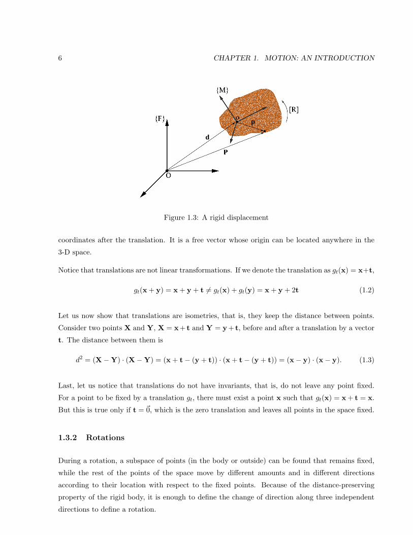
The motion of a rigid body is modeled as the motion of a three-dimensional space. We attach a

coordinate frame to the rigid body, in which the coordinates of points of the body remain fixed

(Figure 1.3).

Every point can be given coordinates with respect to a frame; we use right-handed orthogonal

frames. In Figure 1.3, a point P has coordinates (X1, X2, X3) when measured in frame {F} and

1.3. THE FINITE DISPLACEMENT 5

Figure 1.2: (a) A pure translation and (b) a pure rotation of a rigid body

p = (x1, x2, x3) with respect to frame {M}.

A finite motion is called a displacement. A displacement can be either a translation, a rotation, or

a combination of both. We will see how a general motion can always be seen as a composition of

a rotation and a translation.

A displacement is modeled as the change in the coordinates (in the fixed frame) of the points of

the rigid body when it moves from the original location (when the fixed frame {F} and the moving

frame {M} are coincident) to the final location in space. Equivalently, it can be seen as the change

of coordinates from points expressed in the moving frame {M} to points expressed in the fixed

frame {F}.

1.3.1 Translations

During a translation, all points of the space move by the same amount in the same direction. If the

direction and the magnitude of the translation are given by a non-unitary vector t as in Figure 1.2

(a), a point that had coordinates x in frame {F} before the translation, is transformed to a point

of coordinates

X = x + t (1.1)

in the fixed frame {F} after the translation.

Here, both points and vectors have coordinates in the three-dimensional space; however, they

are different objects. The same vector t is used to transform any point of the space to the new


Figure 1.3: A rigid displacement

coordinates after the translation. It is a free vector whose origin can be located anywhere in the

3-D space.

Notice that translations are not linear transformations. If we denote the translation as gt(x) = x+t,

gt(x + y) = x + y + t 6= gt(x) + gt(y) = x + y + 2t (1.2)

Let us now show that translations are isometries, that is, they keep the distance between points.

Consider two points X and Y, X = x + t and Y = y + t, before and after a translation by a vector

t. The distance between them is

d2 = (X−Y) · (X−Y) = (x + t− (y + t)) · (x + t− (y + t)) = (x− y) · (x− y). (1.3)

Last, let us notice that translations do not have invariants, that is, do not leave any point fixed.

For a point to be fixed by a translation gt, there must exist a point x such that gt(x) = x + t = x.

But this is true only if t = ~0, which is the zero translation and leaves all points in the space fixed.

1.3.2 Rotations

During a rotation, a subspace of points (in the body or outside) can be found that remains fixed,

while the rest of the points of the space move by different amounts and in different directions

according to their location with respect to the fixed points. Because of the distance-preserving

property of the rigid body, it is enough to define the change of direction along three independent

directions to define a rotation.


Intuitively, we can consider two different entities associated to rigid bodies: directions and points.

Directions are free vectors and hence translations have no effects on them; however, they can be

transformed by rotations. On the other hand, points are transformed by translations and also by

rotations.

We attach a moving frame {M} to a point of the rigid body, see Figure 1.2 (b). The orientation

of the body is defined as the coordinates of the three perpendicular vectors that form the moving

frame, expressed in the fixed frame.

The most common way of representing rotations is by using matrices. The matrix that contains

the expression of the column vectors of the moving frame {x,y, z} expressed in the fixed frame,

[R] =[x y z

], (1.4)

defines the rotation from an initial position in which the fixed and moving frames were coincident,

to the final position of the moving frame. At the same time, the matrix [R] defines also the change in

coordinates from points of the body expressed in coordinates of the moving frame, to the expression

of the same point in the fixed frame, see Figure 1.3. A point that had coordinates x (expressed in

the fixed frame) before the rotation, is transformed to a point of coordinates

X = [R]x (1.5)

after the rotation. That is, if Ei is the basis vector ei of the moving frame expressed in the fixed

frame,

[R]x = [R](x1e1+x2e2+x3e3) =[E1 E2 E3

](x1

100

+x2

010

+x3

001

) = x1E1+x2E2+x3E3.

(1.6)

Rotations are linear transformations. If we denote the transformation as r(x) = [R]x,

r(x + y) = [R](x + y) = [R]x + [R]y = r(x) + r(y). (1.7)

Because we are using orthonormal frames, the rotation matrix is an orthogonal matrix, that is, its

columns are mutually orthogonal and unitary. This, together with the fact that we use right-handed

frames, leads to the result:

Proposition 1.3.1 A rotation matrix satisfies the following properties:

• [R][R]T = [R]T [R] = [I]


• det[R] = +1

Proof: Exercise.

Let us check now that rotations are isometries. Consider X = [R]x and Y = [R]y being two pointstransformed by the same rotation. The distance between them is

(X−Y) · (X−Y) =([R]x− [R]y) · ([R]x− [R]y) = ([R](x− y)) · ([R](x− y)) =

([R](x− y))T ([R](x− y)) = (x− y)T [R]T [R](x− y) = (x− y) · (x− y)(1.8)

We can use our knowledge of matrix algebra to determine whether there are points that remainfixed during a rotation (they are called invariants) and how to find these points.

Let us look at the eigenvalues of [R]. A scalar λ is an eigenvalue of a matrix [R] if [R]x = λx. Toobtain some information about their values, we can compute the length of the eigenvector beforeand after the transformation. For doing that, we compute the dot product; if we transpose theabove expression (taking into account that λ may be a complex number), and we multiply themtogether, we obtain

xT [R]T [R]x = λλxTx, (1.9)

and using the fact that [R]T [R] = [I] and λλ = |λ|2,

|λ|2 = 1 (1.10)

for all λ being an eigenvalue of the rotation matrix. This, together with the fact that det[R] =λ1λ2λ3 = +1, leaves us with the following eigenvalues:

Proposition 1.3.2 A three-dimensional rotation matrix has the following eigenvalues:

• λ1 = 1

• λ2 = eiθ

• λ3 = e−iθ

Proof: See the construction above. For a different construction involving the characteristic poly-nomial of the rotation matrix, see [14].

A fixed point will have the same coordinates before and after the transformation, that is,

[R]x = x. (1.11)

From here we have([R]− [I])x = ~0. (1.12)


The obvious solution is x = ~0, which tells us that the origin is an invariant. A possible subspace offixed points exists if det([R]− [I]) = 0. This is always true, as we know that one of the eigenvaluesof [R] is λ1 = 1. We will find not a point, but a whole direction of points being invariants. Theonly other possibility of fixed points is when the other two eigenvalues also become equal to 1; inthat case we get the identity matrix. We know that the direction of fixed points includes the origin;it is called the rotation axis and it can be found using Cayley’s formula. For the derivation of thisformula we follow [15].

We start with the length-preserving property of rotations as seen in Eq.(1.9). We can express it asX ·X− x · x = 0. This is transformed to

(X− x) · (X + x) = 0, (1.13)

so that the addition and difference vectors are perpendicular. Notice that, if we express X = [R]x,we obtain the expression,

X− x = [R− I][R+ I]−1(X + x). (1.14)

We define the matrix[B] = [R− I][R+ I]−1. (1.15)

By construction we have seen that applying [B] to a vector y makes it perpendicular. Hence,yT [B]y = 0. From this equation we can see that [B] is a skew-symmetric matrix, that is, [B]T =−[B] and its elements are

[B] =

0 −b3 b2

b3 0 −b1−b2 b1 0

. (1.16)

The only three different elements of the matrix can be assembled in the vector b = (b1, b2, b3), andthe matrix product with [B] can be substituted by the vector cross product, [B]y = b× y.

From Eq.(1.15) we can derive the expression of [R] as a function of [B], also known as Cayley’sformula,

[R] = [I −B]−1[I +B]. (1.17)

When we substitute this expression in Eq.(1.11), we obtain

[B]x = 0, (1.18)

hence b × x = 0, which means that b is a solution of the fixed point equation. The rotation axisis given by the direction of vector b.

The set of invariant points that form the direction b defines the rotation axis and it is also calledRodrigues’ vector. It can also be shown that the length of this vector is |b| = tan φ

2 , where φ is therotation angle about the rotation axis. We usually write b = tan φ

2 s, where s is the unit direction,or rotation axis.


The following relation between the skew-symmetric matrix [B] and the rotation matrix [R] is alsouseful,

[R− I] =2

1 + tan2 φ2

([B]− [B]T [B]). (1.19)

1.3.3 General finite displacements

A general finite displacement can be always described as a composition of a translation and arotation. In this context, composition means just the concatenation of two transformations, onerealized after the other. We will formalize this within the context of group theory.

We will write the general displacement gT as composed of a rotation by an orthogonal matrix [R]and a translation by a vector d,

X = gT (x) = [R]x + d. (1.20)

In this definition we are assuming that the rotation is performed first, followed by the translation,

gT (x) = (gd ◦ gR)(x) = gd(gR(x)) = gd([R]x) = [R]x + d. (1.21)

It is easy to see that the properties of rotation matrices and translation vectors studied above holdfor the general displacement, that is, a general displacement is an isometry, as both translation androtation are isometries, but it is not linear due to the nonlinearity of the translation. We will studythe invariants of a general displacement later; we are now going to derive some formulas that willbe useful for us when dealing with displacements.

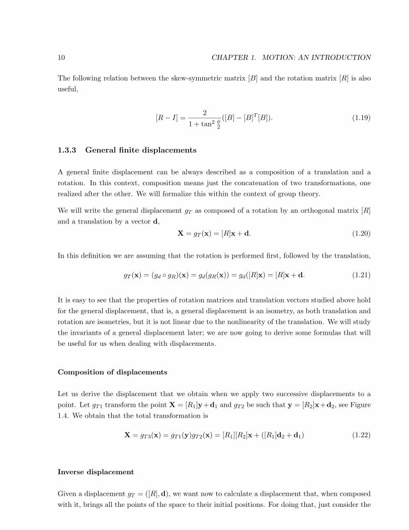
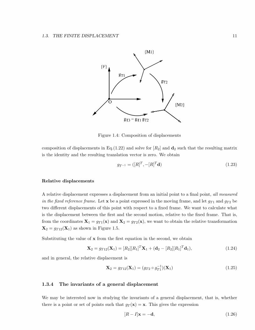
Composition of displacements

Let us derive the displacement that we obtain when we apply two successive displacements to apoint. Let gT1 transform the point X = [R1]y+d1 and gT2 be such that y = [R2]x+d2, see Figure1.4. We obtain that the total transformation is

X = gT3(x) = gT1(y)gT2(x) = [R1][R2]x + ([R1]d2 + d1) (1.22)

Inverse displacement

Given a displacement gT = ([R],d), we want now to calculate a displacement that, when composedwith it, brings all the points of the space to their initial positions. For doing that, just consider the


Figure 1.4: Composition of displacements

composition of displacements in Eq.(1.22) and solve for [R2] and d2 such that the resulting matrixis the identity and the resulting translation vector is zero. We obtain

gT−1 = ([R]T ,−[R]Td) (1.23)

Relative displacements

A relative displacement expresses a displacement from an initial point to a final point, all measuredin the fixed reference frame. Let x be a point expressed in the moving frame, and let gT1 and gT2 betwo different displacements of this point with respect to a fixed frame. We want to calculate whatis the displacement between the first and the second motion, relative to the fixed frame. That is,from the coordinates X1 = gT1(x) and X2 = gT2(x), we want to obtain the relative transformationX2 = gT12(X1) as shown in Figure 1.5.

Substituting the value of x from the first equation in the second, we obtain

X2 = gT12(X1) = [R2][R1]TX1 + (d2 − [R2][R1]Td1), (1.24)

and in general, the relative displacement is

X2 = gT12(X1) = (gT2 ◦ g−1T1 )(X1) (1.25)

1.3.4 The invariants of a general displacement

We may be interested now in studying the invariants of a general displacement, that is, whetherthere is a point or set of points such that gT (x) = x. This gives the expression

[R− I]x = −d, (1.26)


Figure 1.5: A relative displacement

and knowing that λ = 1 is an eigenvalue of the rotation matrix and hence [R − I] is singular, wecan determine that there are no fixed points in a general displacement. However, there is a linewhich is an invariant of the displacement. In order to calculate this line, we need to study someline geometry. We will come back to this calculation after next section.

1.4 A little bit of line geometry

This section is intended as an introduction to become familiar with line geometry. At this point, weare interested in having a good, useful definition of a line in space. Later on we may be interestedin how to define planes, volumes, etc., and we will see that we can do it in a similar fashion.

Lines are heavily used in spatial kinematics, and the reason was pointed out at the end of last sec-tion: for every displacement, we can find an invariant line. We find these invariant lines everywherein mechanisms that perform motion; they usually define where the joints are located.

A line has a direction and it has a location in space. The parameterized expression of a line uses apoint c on the line, a direction vector s and a parameter t, describing the points belonging to theline as

L : c + ts, t ∈ R (1.27)

However, this description is not very good for algebraic operations. We want to determine distancesbetween lines, angles between lines and so on. We use a description of a line called the Pluckercoordinates. They define the line as two vectors, a direction vector and a moment vector,

L = s + εs0 = s + εc× s, (1.28)

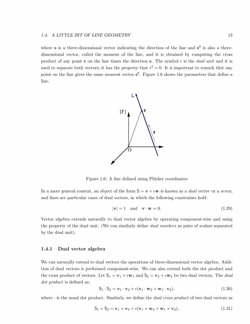
1.4. A LITTLE BIT OF LINE GEOMETRY 13

where s is a three-dimensional vector indicating the direction of the line and s0 is also a three-dimensional vector, called the moment of the line, and it is obtained by computing the crossproduct of any point c on the line times the direction s. The symbol ε is the dual unit and it isused to separate both vectors; it has the property that ε2 = 0. It is important to remark that anypoint on the line gives the same moment vector s0. Figure 1.6 shows the parameters that define aline.

Figure 1.6: A line defined using Plucker coordinates

In a more general context, an object of the form S = v + εw is known as a dual vector or a screw,and lines are particular cases of dual vectors, in which the following constraints hold:

|v| = 1 and v ·w = 0. (1.29)

Vector algebra extends naturally to dual vector algebra by operating component-wise and usingthe property of the dual unit. (We can similarly define dual numbers as pairs of scalars separatedby the dual unit).

1.4.1 Dual vector algebra

We can naturally extend to dual vectors the operations of three-dimensional vector algebra. Addi-tion of dual vectors is performed component-wise. We can also extend both the dot product andthe cross product of vectors. Let S1 = v1 + εw1 and S2 = v2 + εw2 be two dual vectors. The dualdot product is defined as:

S1 · S2 = v1 · v2 + ε(v1 ·w2 + w1 · v2), (1.30)

where · is the usual dot product. Similarly, we define the dual cross product of two dual vectors as

S1 × S2 = v1 × v2 + ε(v1 ×w2 + w1 × v2), (1.31)


where × is the usual cross product of three-dimensional vectors.

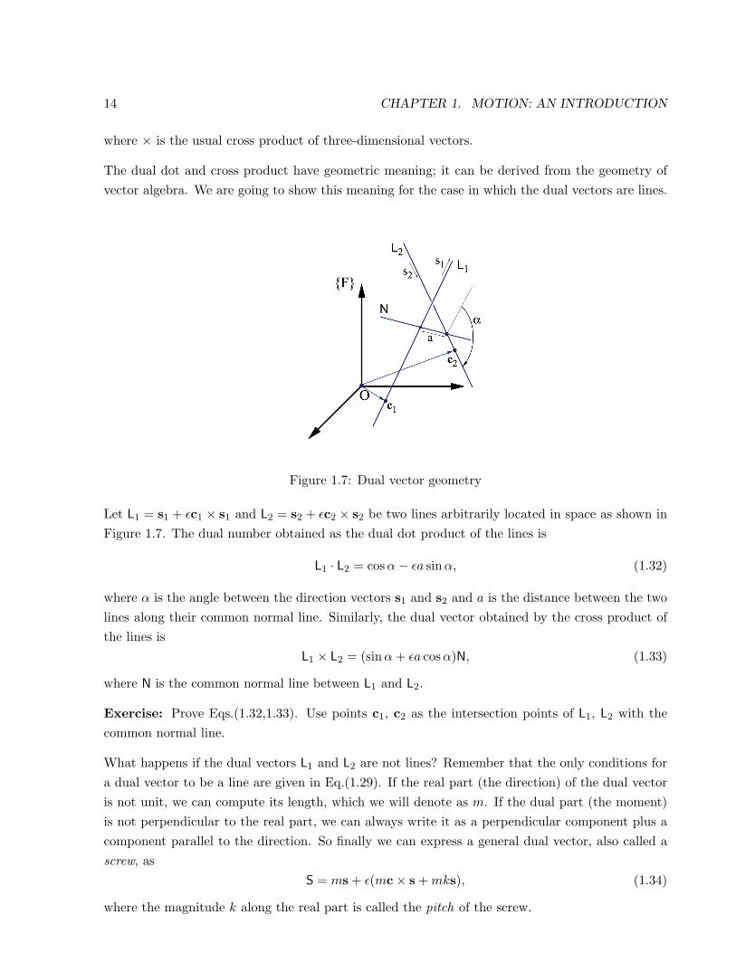
The dual dot and cross product have geometric meaning; it can be derived from the geometry ofvector algebra. We are going to show this meaning for the case in which the dual vectors are lines.

Figure 1.7: Dual vector geometry

Let L1 = s1 + εc1 × s1 and L2 = s2 + εc2 × s2 be two lines arbitrarily located in space as shown inFigure 1.7. The dual number obtained as the dual dot product of the lines is

L1 · L2 = cosα− εa sinα, (1.32)

where α is the angle between the direction vectors s1 and s2 and a is the distance between the twolines along their common normal line. Similarly, the dual vector obtained by the cross product ofthe lines is

L1 × L2 = (sinα+ εa cosα)N, (1.33)

where N is the common normal line between L1 and L2.

Exercise: Prove Eqs.(1.32,1.33). Use points c1, c2 as the intersection points of L1, L2 with thecommon normal line.

What happens if the dual vectors L1 and L2 are not lines? Remember that the only conditions fora dual vector to be a line are given in Eq.(1.29). If the real part (the direction) of the dual vectoris not unit, we can compute its length, which we will denote as m. If the dual part (the moment)is not perpendicular to the real part, we can always write it as a perpendicular component plus acomponent parallel to the direction. So finally we can express a general dual vector, also called ascrew, as

S = ms + ε(mc× s +mks), (1.34)

where the magnitude k along the real part is called the pitch of the screw.

1.4. A LITTLE BIT OF LINE GEOMETRY 15

1.4.2 More line geometry

Sometimes we may be interested in computing a point in the line, given its Plucker coordinates.This can be done in general, for a screw S = v + εw,

c =v ×wv · v

. (1.35)

We can see how it works: take the general expression of a screw in Eq.(1.34), and let us computethe cross product of w = mc× s +mks by v = ms,

ms× (mc× s +mks) = m2s× (c× s) +m2ks× s. (1.36)

Now we apply the identity a× (b× c) = ba · c− ca · b to obtain

m2s× (c× s) = m2(c(s · s)− s(s · c)) = m2c (1.37)

if we consider c as the point perpendicular to the direction s - remember that we can take any pointon the line. Notice also that m2 is the dot product of the direction of the dual vector by itself.

The fact that any point can be used to compute the moment of the line can be easily seen: imaginethat c is the point on the line perpendicular to the direction, and consider now the point k = c+ tswhich has a component along the direction s. Compute the moment of the line using k,

k× s = (c + ts)× s = c× s + ts× s = c× s. (1.38)

The component along the direction does not contribute to the moment.

From all the information on this section we can define how to compute the common normal line,the line which is perpendicular to two given lines. Using Eq.(1.33), we obtain a screw which isperpendicular to both lines. In order to make it a line,

• Make the direction a unit vector, n.

• Find a point p in the screw as indicated above.

• Construct the common normal line as N = n + εp× n.

1.4.3 Line motion

A question that relates to our interests is, how do we specify the motion of a line? We need tobe able to apply a displacement to a line and obtain the displaced line. One way is to use therotation matrix to compute the change in orientation of the direction, and apply separately thedisplacement to a point on the line, assembling the Plucker coordinates of the line afterwards. Wecan also create a matrix that captures all these operations.


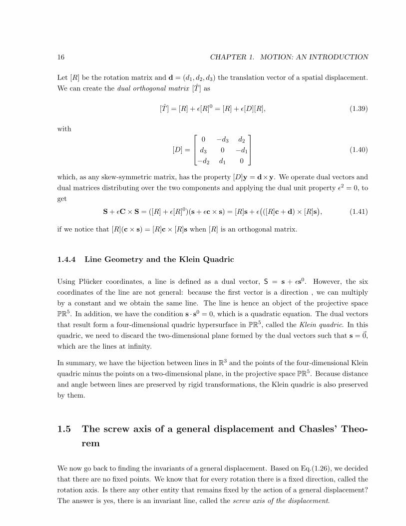
Let [R] be the rotation matrix and d = (d1, d2, d3) the translation vector of a spatial displacement.We can create the dual orthogonal matrix [T ] as

[T ] = [R] + ε[R]0 = [R] + ε[D][R], (1.39)

with

[D] =

0 −d3 d2

d3 0 −d1

−d2 d1 0

(1.40)

which, as any skew-symmetric matrix, has the property [D]y = d×y. We operate dual vectors anddual matrices distributing over the two components and applying the dual unit property ε2 = 0, toget

S + εC× S = ([R] + ε[R]0)(s + εc× s) = [R]s + ε(([R]c + d)× [R]s

), (1.41)

if we notice that [R](c× s) = [R]c× [R]s when [R] is an orthogonal matrix.

1.4.4 Line Geometry and the Klein Quadric

Using Plucker coordinates, a line is defined as a dual vector, S = s + εs0. However, the sixcoordinates of the line are not general: because the first vector is a direction , we can multiplyby a constant and we obtain the same line. The line is hence an object of the projective spacePR5. In addition, we have the condition s · s0 = 0, which is a quadratic equation. The dual vectorsthat result form a four-dimensional quadric hypersurface in PR5, called the Klein quadric. In thisquadric, we need to discard the two-dimensional plane formed by the dual vectors such that s = ~0,which are the lines at infinity.

In summary, we have the bijection between lines in R3 and the points of the four-dimensional Kleinquadric minus the points on a two-dimensional plane, in the projective space PR5. Because distanceand angle between lines are preserved by rigid transformations, the Klein quadric is also preservedby them.

1.5 The screw axis of a general displacement and Chasles’ Theo-

rem

We now go back to finding the invariants of a general displacement. Based on Eq.(1.26), we decidedthat there are no fixed points. We know that for every rotation there is a fixed direction, called therotation axis. Is there any other entity that remains fixed by the action of a general displacement?The answer is yes, there is an invariant line, called the screw axis of the displacement.

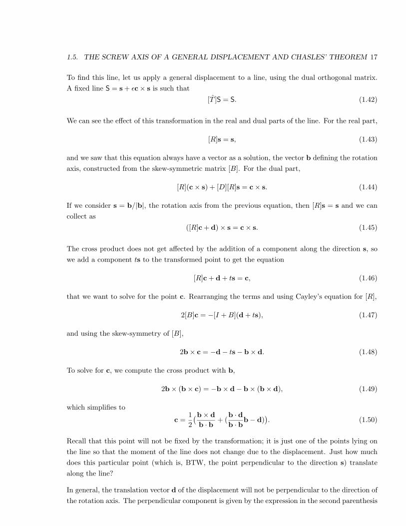
1.5. THE SCREW AXIS OF A GENERAL DISPLACEMENT AND CHASLES’ THEOREM 17

To find this line, let us apply a general displacement to a line, using the dual orthogonal matrix.A fixed line S = s + εc× s is such that

[T ]S = S. (1.42)

We can see the effect of this transformation in the real and dual parts of the line. For the real part,

[R]s = s, (1.43)

and we saw that this equation always have a vector as a solution, the vector b defining the rotationaxis, constructed from the skew-symmetric matrix [B]. For the dual part,

[R](c× s) + [D][R]s = c× s. (1.44)

If we consider s = b/|b|, the rotation axis from the previous equation, then [R]s = s and we cancollect as

([R]c + d)× s = c× s. (1.45)

The cross product does not get affected by the addition of a component along the direction s, sowe add a component ts to the transformed point to get the equation

[R]c + d + ts = c, (1.46)

that we want to solve for the point c. Rearranging the terms and using Cayley’s equation for [R],

2[B]c = −[I +B](d + ts), (1.47)

and using the skew-symmetry of [B],

2b× c = −d− ts− b× d. (1.48)

To solve for c, we compute the cross product with b,

2b× (b× c) = −b× d− b× (b× d), (1.49)

which simplifies to

c =12(b× d

b · b+ (

b · db · b

b− d)). (1.50)

Recall that this point will not be fixed by the transformation; it is just one of the points lying onthe line so that the moment of the line does not change due to the displacement. Just how muchdoes this particular point (which is, BTW, the point perpendicular to the direction s) translatealong the line?

In general, the translation vector d of the displacement will not be perpendicular to the direction ofthe rotation axis. The perpendicular component is given by the expression in the second parenthesis


in Eq.(1.50). The component parallel to the rotation axis is given by its projection and will definethe amount of slide along the line. We can write

t =b · d|b|

. (1.51)

Chasles’ theorem can be used to summarize the results of this section. Figure 1.8 shows theequivalent descriptions of a displacement.

Figure 1.8: The screw axis, rotation angle and slide of a displacement

Theorem 1.5.1 (Chasles, approx. 1830). A general displacements in 3-dimensional space is equiv-alent to a screw motion consisting of a rotation of angle φ about and a translation t along a lineS = s + εs0.

The direction s and rotation angle φ are computed from the rotation. The moment vector s0 andthe slide are computed using the equations just derived above. In total, we need to define sixparameters: four to define the direction and location of the line, and two to define the rotation andslide values. The screw axis is a very efficient way of representing a general displacement.

1.6. MORE ON MATRIX REPRESENTATION 19

1.6 More on Matrix Representation

1.6.1 How to create a rotation matrix

When we covered rotations, we defined the rotation matrix as containing as columns the coordinatesof the vectors of the moving frame, expressed in the fixed frame. This description, even thoughcorrect, may be of little practical use when we want to compute the matrix defining a rotation.

Methods to generate a rotation matrix include: Euler angles, roll-pitch-yaw angles, longitude-latitude-roll angles, product of two reflections, use of the rotation axis and rotation angle. We willcover here Euler angles and the use of the rotation axis; for more information, see [11] or [7].

Euler angles

A rotation about one of the coordinate axes of the fixed frame adopts a very simple expressionand it is also easy to visualize. The coordinate rotations about axes X, Y and Z are given by thematrices

[X(α)] =

1 0 00 cosα − sinα0 sinα cosα

[Y (β)] =

cosβ 0 sinβ0 1 0

− sinβ 0 cosβ

[Z(θ)] =

cos θ − sin θ 0sin θ cos θ 0

0 0 1

.(1.52)

We can create a general rotation as the composition of three rotations about perpendicular axes.We could use X− Y − Z,

[R(α, β, θ)] = [X(α)][Y (β)][Z(θ)], (1.53)

or any other combination, like Z− Y − Z. Notice that the first rotation happens about X, and thesecond rotation is about the rotated Y axis, not the original one, and the third rotation is aboutan axis Z that has been transformed by the two previous rotations; see Figure 1.9.

A somehow similar way of describing a rotation is by using three coordinate rotations about fixedaxis. See [11] for a description of this method.

Equivalent axis-angle representation and Euler parameters

We proved in section 1.3.2 that a rotation can be characterized by the rotation axis and rotationangle about the axis. Using Cayley’s equation, we can express the components of the rotation matrixas a function of the parameters of the vector b. Recall that b = (b1, b2, b3) = tan φ

2 (sx, sy, sz). We


Figure 1.9: Euler angles

obtain

[R] = [I −B]−1[I +B] =1

1 + b21 + b22 + b23

1 + b21 − b22 − b23 2(b1b2 − b3) 2(b1b3 + b2)2(b1b2 + b3) 1− b21 + b22 − b23 2(b2b3 − b1)2(b1b3 − b2) 2(b2b3 + b1) 1− b21 − b22 + b23

(1.54)

We can see that using the invariant axis and angle to define the rotation matrix gives a not sosimple expression. There is a similar expression of the rotation matrix as a function of the rotationaxis and angle. If we multiply vector b by cos φ2 , with cos φ2 6= 0, we can define the following fourcoefficients, which are called the Euler parameters of the rotation,

c1 = cosφ

2b1 = sin

φ

2s1,

c2 = cosφ

2b2 = sin

φ

2s2,

c3 = cosφ

2b3 = sin

φ

2s3,

c0 = cosφ

2. (1.55)

The rotation matrix can be written then as

[R] =1

c20 + c21 + c22 + c23

c20 + c21 − c22 − c23 2(c1c2 − c0c3) 2(c1c3 + c0c2)2(c1c2 + c0c3) c20 − c21 + c22 − c23 2(c2c3 − c0c1)2(c1c3 − c0c2) 2(c2c3 + c0c1) c20 − c21 − c22 + c23

(1.56)

These parameters will be revisited when we study Clifford algebras.


1.6.2 Homogeneous matrix representation

The homogeneous matrix representation is a convenient (and meaningful, as we will see later indetail) way of describing a general displacement. Given a displacement gT = ([R],d), we can createthe 4× 4 homogeneous transform as

[T ] =

|

[R] | d− − − −|− −0 0 0 | 1

. (1.57)

This four-dimensional matrix contains all the information about the displacement. In order tomatch the dimensions, we need to add a fourth component to our vectors. Notice that we aretransforming two types of things with a general displacement: we transform points (their position)and we also transform directions. Up until now, we have treated these two in the same man-ner, as three-dimensional vectors, even though we knew that they were different things. In thehomogeneous representation, they will have also different expressions.

For transforming position of points, we will add a unit as the last element of the vectors, so thatX1

X2

X3

1

= [T ]

x1

x2

x3

1

. (1.58)

For transforming directions, we will add zero as the last element,X1

X2

X3

0

= [T ]

x1

x2

x3

0

. (1.59)

We will cover the geometric explanation of this fourth component in subsequent sections dealingwith projective geometry. For our purpose now, the addition of that last component allows us tooperate a displacement by using a single matrix. The expressions found above for composition ofdisplacements, inverse displacement and relative displacement hold, that is,

Composition: X = gT3(x) = gT1(y)gT2(x) = [T1][T2]x,

Inverse: x = gT−1(X) = (gT )−1(X) = [T ]−1X,

Relative displacement: X2 = gT12(X1) = (gT2g−1T1 )(X1) = [T2][T1]−1X1. (1.60)

Exercise: Check that the rotation matrix and displacement vector obtained with the 4×4 homoge-neous matrix for the composition of displacements, inverse displacement and relative displacementare the same as the ones derived above.


We denote a rotation and a translation about and along an axis as a screw displacement. The screwdisplacements along the coordinate axes X, Y and Z take a simple form,

[X(α, a)] =

1 0 0 a

0 cosα − sinα 00 sinα cosα 00 0 0 1

[Y (β, b)] =

cosβ 0 sinβ 0

0 1 0 b

− sinβ 0 cosβ 00 0 0 1

(1.61)

and

[Z(θ, t)] =

cos θ − sin θ 0 0sin θ cos θ 0 0

0 0 1 t

0 0 0 1

. (1.62)


Homework 1

Chapter 1

1. Prove that the rotation matrix satisfies the properties stated in Proposition 1.3.1.

2. Write the matrix (using Euler angles) corresponding to the following rotation: a rotationabout the Z axis of 30o, followed by a rotation about the Y axis of 40o, followed by anotherrotation about the Z axis of −35o. Find the rotation axis and the rotation angle about thisaxis.

3. Show that, for a general displacement gT , gT (x + y) 6= gT (x) + gT (y).

4. Show that a general displacement is an isometry.

5. Write a 4× 4 homogeneous matrix representing the following displacements of a spoon: fromthe side of the plate to a resting position inside of the soup, and from this second position tothe mouth.

6. Check that the results of the composition of displacements, inverse displacement and relativedisplacement hold when using the 4× 4 homogeneous transform.

7. Compute the composition of displacements of problem 5.

8. Prove that a point in the line S = v + εw (in fact, the point of intersection with the perpen-dicular line from the origin) can be found as c = v×w

v·v .

9. Compute the invariants (screw axis, rotation about and translation along it) of the displace-ment in problem 7.

10. Compute the common normal line, and the distance and angle between the following lines:L1 = (0.82, 0.41, 0.41) + ε(−1.22, 1.22, 1.22) and L2 = (0.45, 0, 0.89) + ε(0.89, 0.89,−0.45)

Bibliography

[1] Ablamowicz, R. and Sobczyk, G., Lectures on Clifford (Geometric) Algebras and Applicatons,Birkhauser, Boston 2004.

[2] Artin, M., Algebra, Prentice-Hall, New Jersey, 1991.

[3] Bayro Corrochano, E., Daniilidis, K., and Sommer, G., “Motor Algebra for 3D Kinematics:The Case of Hand-Eye Calibration”, Journal of Mathematical Imaging and Vision, 13:79-100,2000.

[4] Bayro Corrochano, E., Geometric Computing for Perception Action Systems, Springer-Verlag,New York, 2001.

[5] Bayro Corrochano, E., Handbook of Geometric Computing, Springer-Verlag, Berlin, 2005.

[6] Bayro-Corrochano, E., and Zamora-Esquivel, J., “Differential and Inverse Kinematics of RobotDevices Using Conformal Geometric Algebra”, Robotica, 25:43-61, 2007.

[7] Bottema, O., and Roth, B., Theoretical Kinematics, North Holland Press, NY, 1979.

[8] Browne, J., Grassmann Algebra: Exploring applications of extended vector algebra withMathematica, Swinburne University of Technology, Melbourne, Australia, 2001. (Draft fromhttp://www.ses.swin.edu.au/homes/browne/grassmannalgebra/book/index.htm).

[9] Cohn, P.M., Algebra, 2nd. edition, John Wiley & Sons, 1989.

[10] Ge, Q.J., 2002, “Projective convexity in computational kinematic geometry”, Proceedings ofthe ASME Design Engineering Technical Conference, pages 715-723, Montreal, Canada, 2002.

[11] Craig, J. J., Introduction to Robotics, Mechanics and Control, Addison Wesley Publ. Co., 1989.

[12] Gosselin, C.M., St-Pierre, E. and Gagne, M., 1996, “On the development of the agile eye: me-chanical design, control issues and experimentation”, IEEE Robotics and Automation SocietyMagazine, 3(4):29-37.

[13] Kumar, A., and Waldron, K.J., 1981, “The Workspace of a Mechanical Manipulator,” ASMEJ. Mech. Design, 103: 665-672.

73

74 BIBLIOGRAPHY

[14] McCarthy, j.m., Introduction to Theoretical Kinematics, The MIT Press, 1990.

[15] McCarthy, J.M., Geometric Design of Linkages, Springer, New York 2000.

[16] Murray, R., Li, Z. and Sastry, S., A Mathematical Introduction to Robotic Manipulation, CRCPress, Boca Raton, 1994.

[17] Perez, A. and McCarthy, J. M., 2005, “Clifford Algebra Exponentials and Planar LinkageSynthesis Equations”,ASME Journal of Mechanical Design, 127(5): 931-940.

[18] Porteous, I. R.,Clifford Algebras and the Classical Groups, Cambridge Studies on AdvancedMathematics, 50, Cambridge University Press, Cambridge, 1995.

[19] Releaux, F., 1875, The Kinematics of Machinery: Outlines of a Theory of Machines, DoverPublications, New York, translation of 1963.

[20] Selig, J.M., Geometrical Methods in Robotics, Springer, London 1996.

[21] Selig, J.M., Geometric Fundamentals of Robotics, Springer, London, 2005.

[22] Sommer, G., Geometric Computing with Clifford Algebras, Chapter1, Springer, Berlin, 2001.

[23] Sugimoto, K., 1987, “Kinematic and Dynamic Analysis of Parallel Manipulators by Means ofMotor Algebra”, ASME Journal of Mechanisms, Transmissions and Automation in Design,109(1):3-5.

[24] Tsai, L. W., 1999, Robot Analysis: The Mechanics of Serial and Parallel Manipulators, JohnWiley and Sons, New York, NY.

Documents

Kinematics of Robots - Idaho State Universityperealba/courses/KinematicsNotes/Chapter1.pdf · 2 Robot Kinematics Using Matrix Algebra 25 ... 8.7 Planar motion and planar geometry: