Embed Size (px)
Citation preview
KoPA
IR
WRrgeiut
*
†
‡A
0d
inetic Modeling in Supportf Radionuclide Dose Assessment
aolo Vicini, PhD,* A. Bertrand Brill, MD, PhD,† Michael G. Stabin, PhD, CHP,† andldo Rescigno, PhD‡
In this review, we trace the origins of mathematical modeling methods and pay particularattention to radiotracer applications. Nuclear medicine has been advanced greatly by theefforts of the Society of Nuclear Medicine’s Medical Internal Radiation Dose Committee.Well-developed mathematical methods and tools have been created in support of a widerange of applications. Applications of mathematical modeling extend well beyond biologyand medicine and are essential to analysis is a wide range of fields that rely on numericalpredictions, eg, weather, economic, and various gaming applications. We start with thediscovery of radioactivity and radioactive transformations and illustrate selected applica-tions in biology, physiology, and pharmacology. We discuss compartment models as toolsused to frame the context of specific problems. A definition of terms, methods, andexamples of particular problems follows. We present models of different applications withvarying complexity depending on the features of the particular system and function beinganalyzed. Commonly used analysis tools and methods are described, followed by estab-lished models which describe dosimetry along gastrointestinal and urinary excretory path-ways, ending finally with a brief discussion of bone marrow dose. We conclude pointing tomore recent, promising methods, not yet widely used in dosimetry applications, which aimat coupling pharmacokinetic data with other patient data to correlate patient outcome(benefits and risk) with the type, amount, kind and timing of the therapy the patientreceived.Semin Nucl Med 38:335-346 © 2008 Published by Elsevier Inc.
hsafmitud
TRwlsl(tsm
ntroductionadioactivity
ithin a year of Roentgen’s discovery of x-rays, Becque-rel discovered naturally occurring radioactivity and
utherford described the laws that govern the kinetics ofadioactive transformations. Human use of radioactivity be-an immediately, and within a few years undesired radiationffects were noted and the need for measuring and monitor-ng dose was recognized. The need for guidance on the safese of radiations led in 1928 to the formation of the Interna-ional Commission on Radiation Protection (ICRP),1 which
Resource Facility for Population Kinetics, Department of Bioengineering,University of Washington, Seattle, WA.
Department of Radiology and Radiological Sciences, Vanderbilt University,Nashville, TN.
Stillwater, MN.ddress reprint requests to Paolo Vicini, Resource Facility for Population
Kinetics, Department of Bioengineering, Box 355061, University ofWashington, Seattle, WA 98195-4290. E-mail: [email protected].
cedu
001-2998/08/$-see front matter © 2008 Published by Elsevier Inc.oi:10.1053/j.semnuclmed.2008.05.007
as since coordinated the worldwide development and dis-emination of radiation-protection guidelines. The methodsnd procedures for calculating dose developed more rapidlyor externally administered radiations than for internally ad-inistered radioactivity, which only later came into increas-
ng use. Internal dosimetry is inherently more complex, ashe radioactive source moves between organs, decaying andndergoing changes that influence the local and remote doseistribution.
racer Modelsadioactivity provided an important advantage because,hen used in minute quantities, it was able to trace the fate of
abeled substances in an organism with exquisitely high sen-itivity without perturbing the system. In general, a tracer is aabel attached to a labeled substance (the tracee). The labeltracer) follows the labeled substance (tracee) because it hashe same mechanical or chemical or biological properties. Inhort, a tracer must have 3 fundamental properties: (1) itust have the same phenomenological properties of the tra-
ee, (2) it must be added to the tracee in a quantity that does
335

ns
tasdgdrsb
taayptunttci
aTmptestlasmot
BTbustlmnpsemmaw
bso
DDtmasteasmaupjrtotsptantppRcfvpc
ppmtsvtmsyc(dtCmid
336 P. Vicini et al
ot alter its behavior, and (3) it must be easily detected as aeparate entity.
In a lighter tone, we mention an early example of the use ofracers. The fictional character Gian Burrasca,2 well known toll Italian children, suspects that the tasty soup his boardingchool serves every Friday, is prepared by rinsing the dirtyishes of the previous week; to make sure of it, he adds a fewrains of aniline to each dish he has eaten from in the last feways. Sure enough, the following Friday the soup is brighted! The Hungarian physicist George de Hevesy reported aimilar anecdote in which he traced the leftover food at hisoarding house to hash served the following day.More scientifically, in 1913 de Hevesy developed the
racer concept when he used the naturally occurring radio-ctive element 210Pb (Ra D) as a tracer in chemistry studies,nd in 1923 to trace the movement of 212Pb in plants and 1ear later 210Bi in animals.3 When linked to biologically im-ortant molecules by means of innovative radiochemistry,hese radioactive isotopes served as tracers leading to newnderstanding of physiological processes. For Hevesy’s pio-eering studies, he was awarded a Nobel Prize in 1943. Afterhe discovery of artificially produced radioactivity in 1934 byhe Joliot Curies, a wide range of radioactive elements be-ame available from the early cyclotrons, and they were usedn many pioneering biologically important investigations.
Tracers are labeled substances that are given in smallmount with respect to the native substance being studied.he intent of the tracer experiment can be to learn about theetabolism of the tracee, or to achieve diagnosis. The tem-oral and spatial distribution of different tracers depends onhe nature of the nuclide and its attached compound, how itnters the body, and the nature and state of the subject beingtudied. In particular for radiotracers, very small amounts ofracer are administered for diagnostic purposes, whereasarger amounts are given for treatment planning, and ther-py, the latter given with the intent to change the state of theystem for the patient’s benefit. A recent review of tracerodels is provided in Cobelli and coworkers.4 In general,
ne can think of at least the following two classes of models inerms of the applications for which they are to be put.
iological Kinetic Modelsracer–tracee models can be considered a special case ofiological kinetic models. Generally, biological models aresed to simulate and to predict the behavior of a biologicalystem in response to different changes in state: for example,he administration of drugs or other interventions. The bio-ogical applications can be very general, and the most com-
on application involves estimation of physiologically sig-ificant parameters from limited data. Physiologically basedharmacokinetic models are an example application.5 In thisituation, one continually adjusts the model (based on differ-ntial or algebraic equations) until predictions and experi-ental realizations agree, usually based on some predeter-ined statistical criterion of goodness of fit and model
dequacy. The model is considered useful until discrepancies
ith additional data are noted, at which point the model can Ie revised. A model can also be used to simulate, ie, generateynthetic data that can be compared with expectations ortherwise obtained measurements.
osimetry Modelsosimetry models can be construed as a further generaliza-
ion containing elements of both tracer models and biologicalodels. The goal of models used for dosimetry studies is to
chieve statistically adequate agreement between the ob-erved experimental data and model predicted results, withhe end result being useful in the calculation of radiation dosestimates to organs of the body. In this case, one identifiesnd uses the simplest system representation that producesuch results. In summary, the principal goal of biokineticodeling for dosimetry is to obtain the area under the time-
ctivity curve for all organs with measured and significantptake of the tracer. The time–activity curve would be ex-ected to be different for different organs and different sub-
ects and is the primary source of information about absorbedadiation in individual organs. The area under the time-ac-ivity curve, defined as the integral of the time–activity curvever some fixed time (often from zero to infinity), provideshe number of disintegrations that have occurred in the mea-ured region over the interval of integration, and is directlyroportional to the cumulative dose received there. The ac-ual dose distribution, however, may be more complicated,s the energy deposition patterns of different radiations mayeed to be taken into account. The integrals of the radioac-ivity time courses of individual organ are thus a startingoint for the dose transport modeling calculations, whichrovide measures of the absorbed dose. The Medical Internaladiation Dose (MIRD) Committee of the of Society for Nu-lear Medicine was established in 1966 to develop methodsor internal dose analysis, for their dissemination and to pro-ide data on practices that influence their appropriate use inatients. Much information on these developments is dis-ussed elsewhere.6
Data on new tracers are usually obtained initially fromreclinical (ie, animal) experiments, followed by clinical ex-eriments involving human subjects, occasionally supple-ented by in vitro experiments that study specific parts of
he system. The methods for analyzing biokinetic data areeveral and vary from the (computationally) very simple toery complex. Simple methods include direct integration ofhe observed data (which one may argue does not imply aodel at all, but this depends on what the calculation is
upposed to provide) to linear or nonlinear regression anal-sis of the data using an assumed functional form. Moreomplex systems use compartment models to represent thepatho) physiology of the system and the related tracer bio-istribution. In this case, the data are modeled by the solu-ion to a system of differential equations, possibly nonlinear.ompartmental models are one of the most commonly usedeans of formulating and analyzing data from nuclear med-
cine studies. MIRD Pamphlet 12 provides a comprehensiveiscussion of kinetic models for absorbed dose calculations.7
t discusses terminology, the general principles involved in
cctopimcBphoifeat
AMRImdtff
wt
w
am
PBatns
witlt
ct
prettt
waB“
PIdoscmisrfitaTmdis
TTrwacmtTt
dcsomn
CIstco
Kinetic modeling in support of radionuclide dose assessment 337
ompartment modeling, with a series of examples. The dis-ussions we present here on compartment models will usehe terminology promulgated in MIRD 12. Operationally,ne seeks a model with as few compartments as are needed toroduce results consistent with the data, and our experience
s that typically 2 to 3 compartments are sufficient. Theodel selection decision is often based on some parsimony
riterion such as the Akaike Information Criterion8 or theayesian Information Criterion.9 A noncompartmental ap-roach is also possible, but the outcome of this approach isighly dependent on hypotheses regarding the system underbservation, as others have shown. Alternative methods ex-st, including integral equations methods, which we omit inavor of more computationally tractable compartment mod-ls. Next, we focus on historical and practical aspects of cre-ting and analyzing models for use in analysis of radiationracer dosimetry data.
Historical Developmentethodological Perspective
adioactive Disintegrationt can be argued that the first application of compartmentalodels was in physics, specifically to describe radioactiveecay. A review of these models is available elsewhere.10 Afterhe discoveries and experiments by Becquerel,11,12 Ruther-ord and Soddy,13,14 the law of radioactive decay has beenormalized as
dX
dt� �K · X(t) (1)
here X(t) is the quantity of radioactive substance present atime t. The integral solution of this equation is
X(t) � X(t0)e�K(t�t0)
here X(t0) is the initial value of X(t) at time t0.Thus, radioactive decay is modeled as a first order process,
nd this has been verified independently by several experi-ental observations.
hysiologyenke and coworkers15 studied the phenomenon of nitrogenbsorption by, and elimination from, the various tissues viahe lung and circulation. They measured the elimination ofitrogen in human subjects breathing pure oxygen; their re-ults could be represented by the expression
Y � A(1 � e�kt)
here Y is the amount of nitrogen eliminated up to time t, As the total amount of nitrogen contained in the body at time� 0, when the breathing of pure oxygen began, and k the
ogarithmic slope of the curve representing Y as a function ofime.
Behnke and coworkers observed that the value of k de-reases after the first 25 minutes; their explanation was that
he nitrogen is eliminated partly from the body fluid and hartly from fatty tissues, simultaneously but with differentates; during the first part of the experiment the nitrogenlimination from the body fluids is prevalent, whereas laterhe elimination from fatty tissues prevails. A better descrip-ion of the experiment is therefore given by a multiexponen-ial function
Y � B(1 � e�k1t) � C(1 � e�k2t)
here B is the total amount of nitrogen contained in water,nd C the total amount contained in fatty tissues, with A �� C. In more modern terminology, we would call Y the
sum of two compartments”.
harmacologyn 1937, Teorell16,17 reported studies of the in vivo kinetics ofrugs after various modes of administration, where the ideaf compartment became a useful generalization of a state of aubstance characterized by both spatial localization andhemical nature. As it is widely accepted, a multicompart-ental model accounts for spatial heterogeneity by postulat-
ng the presence of different spatial locations where the sub-tance distributes or is transformed. Teorell’s equations foresorption, elimination, tissue uptake, and inactivation wererst-order differential equations whose solutions describinghe amounts of drug in blood and tissue as function of timere sums of exponential terms with constant coefficients.his is of course not exclusive to compartmental systems:ultiexponential decays can also be interpreted as a purelyata-based descriptive approach, as others have pointed out
n distinguishing between “models of data” and “models ofystem.”18
racer Kineticseorell’s work extended the idea of compartment from theadioactivity problem (where it describes a set of particles allith the same probability of transformation) to the physical
nd physicochemical problem. In a 1938 paper, Artom andolleagues19 presented a radioactive tracer study of the for-ation of phospholipids as affected by dietary fat, in which
hey gave a more formal analysis than was provided before.heir equations are also linear constant coefficient differen-
ial equations, and have been reviewed in detail elsewhere.10
In the intervening decades, applications of model-basedata analysis have become widespread and far too many to beounted. Our intent here is only to provide a historical per-pective on the origin of the related concepts and especiallyn the initial intent of the pioneering work at the root of soany current efforts in the fields of systems modeling inuclear medicine, pharmacology, metabolism, etc.
ontinuous Distributionn all examples we have shown so far, the entity under ob-ervation, be it a tracer or a tracee, was supposed to be dis-ributed among a number (small or large, but always finite) ofompartments, each one of them characterized by a functionf time, extensive (mass) or intensive (concentration). This
ypothesis is certainly completely confirmed by the evidence
itiftftadea(
ssnvatwdotlt
CDFpHatlovk1
prompmcatc
OFvab
wptasadet
tce
mttt
wo
aCot
ixrfitrCsc
wttt
338 P. Vicini et al
n the case of radioactive disintegrations, because we knowhat in a radioactive chain one nuclide is transformed into itsmmediate successor without any intermediate steps (at leastrom a macroscopic point of view). In the biological world,he hypothesis of a finite number of compartments leadsrequently, as we have shown above, to a reasonable descrip-ion of the observed events, but there may be cases when thispproximation is no longer valid. An obvious example is theistribution of a drug in the plasma after an IV injection:xcept when the elimination rate is very slow, there willlways be a gradient of c(t) from the site of injection to the siteor sites) of elimination.
In general, to account for the nonuniform distribution of aubstance in an organ, the pertinent function c(t) should beubstituted by a function c(s,t), where s is a spatial coordi-ate; s can be the one-dimensional coordinate along a narrowessel, or a three-dimensional coordinate in a large organ. Inny case, the differential equations used in the previous sec-ions should be replaced by partial differential equationhose solution and parameter estimation is in general quiteifficult, except in some special cases when the contributionf nonexchanging and exchanging vessels can be separatedhanks to the available data, eg, from multiple indicator di-ution. Illuminating examples are described, for example, inhe work by Goresky.20
ompartment Modelsefinition of Compartment
ormal definitions of “compartment” can be found in Shep-ard,21 Sheppard and Householder,22 Rescigno and Segre,23
earon,24 Brownell and coworkers,25 Berman,26 Rescignond Beck,27 Jacquez,28 Gùrpide,29 and Siri.30 Paraphrasinghese authors, a compartment may represent either a physicalocation where a substance resides or a specific chemical statef the substance under study. Nuclear medicine examplesary greatly in complexity. In positron emission tomographyinetic studies,31,32 18F-fluorodeoxyglucose (18F-FDG) and
8F-FDG-6P are different chemical entities which are bothhysically present in the intracellular space: as such, they areepresented as two distinct compartments in kinetic modelsf 18F-FDG studies. More complex models include the Ber-an iodine kinetics model26 which contains thirteen com-
artments, of which eight comprise the thyroid space sub-odel. The thyroid space is modeled with a delay chain of six
ompartments which represent the transition between rapidnd slow clearance phases of iodine transport through thehyroid. In the case of the thyroid, these transitions happen toonstitute a chemical transformation in time and space.
ne-Compartment Modelor practical purposes, in tracer kinetics it is sometimes con-enient to use the following operational definition33: “A vari-ble x(t) of a system is called a compartment if it is governed
y a differential equation of the typedx
dt� �K x(t) � r(t), (2)
ith K constant.” The constant K, as we have seen in therevious sections, may be the rate of radioactive disintegra-ion, or the rate of elimination of a drug, or the probability of
particle passing from its present state to other possibletates.10 The equation is formalized starting from observationnd is usually confirmed by independent experimental evi-ence, like we have mentioned above for biological mod-ls.34-36 Of note, K is always constant in tracer systems if theracee is in a steady state.
In general, moving beyond tracer kinetics, it is possible forhe rate K to be time varying, for instance in systems that areharacterized by saturative behavior. In this case, the differ-ntial equation is nonlinear and has the form
dx
dt� �
Vm
Km � x(t)x(t) � r(t). (3)
Such nonlinear systems can be handled only through nu-erical integration. It is noteworthy to repeat that adminis-
ration of a tracer, by definition, “linearizes” the system, if theracee is at steady state; in fact if eq 3 is valid for the tracee, theracer equation is
dx∗
dt� �
Vm
Km � x(t) � x∗(t)x∗(t) � r(t) � r∗(t),
here x*(t) is the amount of tracer present and r*(t) is its ratef recirculation. But
Vm
Km � x(t) � x∗(t)�
Vm
Km � x(t)
nd the right hand side ratio is constant at tracee steady state.learly, if a compartment is at steady state the turnover timef the tracee is constant; furthermore, tracer and tracee havehe same turnover time by definition.
Eq 2 is a conservation equation (ie, conservation of mass),e, it states that the temporal variation dx/dt of the quantity(t) present in the compartment is the difference between itsate of entry r(t) and its rate of exit. This is in addition to therst order hypothesis. When comparing models such as thiso data, the amount of substance in an organ cannot be di-ectly measured, however its concentration may be available.oncentration values may be calculated by dividing both
ides of eq 2 by an appropriate value for V, the volume of theompartment, providing
dc
dt� �K c(t) �
r(t)
V, (4)
here c(t) � x(t)/V is the concentration of the substance inhe compartment. Note that eq 4 is not a conservation equa-ion, as has been discussed previously.37 Volume of distribu-ion can be calculated using the equation
D
V �c∗(0)(5)

wtttcam
s
w
setts
stbmt
ws
MoMiNttranhtnfeman((pmtnti
mstodtasaandmdmlnDcom
CWdip
F
Kinetic modeling in support of radionuclide dose assessment 339
here c*(0) is the extrapolated value of the concentrationime curve at 0, immediately after a pulse dose. However, inhis case the initial volume of distribution V is not necessarilyhe physical volume of the compartment, as has been dis-ussed previously.37 Thus, the initial volume of distribution,s defined by eq 5, cannot be considered an absolute phar-acokinetic parameter.38
If we multiply and divide the first term of the right-handide of eq 2 by V we get
dx
dt� �VK · c(t) � r(t); (6)
here the extensive term VK is clearance, Cl.Explicit integration of the differential equations to recon-
truct c(t) is only possible in very simple cases. However,ven if we don’t have sufficient data to reconstruct the func-ion x(t) or c(t), we can extract some partial information onhe system under study, as we shall show in the next fewections.
In general, suppose that the substance or tracer undertudy is distributed among n compartments, but only one ofhem can be sampled, and that its concentration c1(t), after aolus administration there at time t � 0, can be approxi-ated reasonably well by a sum of exponential functions;
hen
c1(t) � A1e��1t � A2e��2t � · · · � Ane��nt
hich is also the general solution to some n-compartmentalystems characterized by linear kinetics.
odeling in Supportf Radiotracer Dosimetryodel complexity ranges from early one compartment stud-
es designed to test red blood cell membrane permeability toa and K ions.39 Compartment models are adequate descrip-
ors, easily amenable to either analytical or numerical solu-ion for such systems. Modeling of thyroid iodine metabolismequires at least three compartments.40 Depending on thepplication and the available data, 13 compartments wereeeded by Berman to analyze fundamental aspects of thyroidormone metabolism. When the system being studied is ex-ended to include pregnant females, 22 compartments wereeeded to include radioiodine kinetics including maternaletal exchange.41 Although explicit analytic methods are ad-quate to calculate the system parameters for 1 to 3 compart-ent systems, more complex models even for dosimetry usu-
lly require use of computer-based analysis tools andumerical analysis, both for calculating model predictionssimulation) and estimating model parameters from dataidentification). Given limited data from individual subjects,atient specific model estimates derived from multicompart-ent models assume default values for many, if not most of
he transport parameters. More recent techniques, such asonlinear mixed effects models, could in principle help avoidhis problem, although they also tend to be quite computer
ntensive. iPractical guidance on the design and analysis of experi-ents using modeling approaches was given by Berman in a
eminal reference.42 In it, Berman discusses factors relating tohe type and class of models. The choice of models is basedn the intended purpose of the model (ie, to describe theata, describe the response of a system to a stimulus, simulatehe system, or to characterize changes in the system). Therticle outlines how computers can be used to obtain best fitolutions to the defining equations. Analysis of plasma clear-nce or whole body turnover data are used as examples inssessing the number of exponential terms, and hence theumber of compartments needed to obtain a good fit to theata. Compartment models are then discussed in terms ofodel known and model unknown circumstances, with aiscussion of the problems relating to the uniqueness ofodel solutions. Elsewhere, Berman shows how the equiva-
ence of results from properly analyzed compartmental andoncompartmental data are essentially indistinguishable.43,44
i Stefano has also discussed elsewhere the properties ofompartmental and noncompartmental systems and modesf analysis, and the circumstances where such approachesay give comparable results.45,46
ompartmental Model Examplese will now describe compartmental models of increasing
etail to illustrate the range of complexity that has been usedn radiation dosimetry in the analysis of medically significantroblems from nuclear medicine.
1. A simple 3-compartment model (Fig. 1) was widely usedin studies to describe thyroid uptake and turnover.47
2. Johansson and coworkers48 extended the iodine model
igure 1 Schematic representation of a 3-compartment model for
odine metabolism.
ar
tTbSSmWgmplrlAuacsdr
SUIrico
DObftmppiip
Fi
340 P. Vicini et al
to calculate dose to other iodine concentrating organsas indicated in Fig. 2. See paper for rate constants and“residence times.”
3. The metabolism of the different thyroid hormones wasdescribed by Berman using an 11 compartment model(Fig. 3).
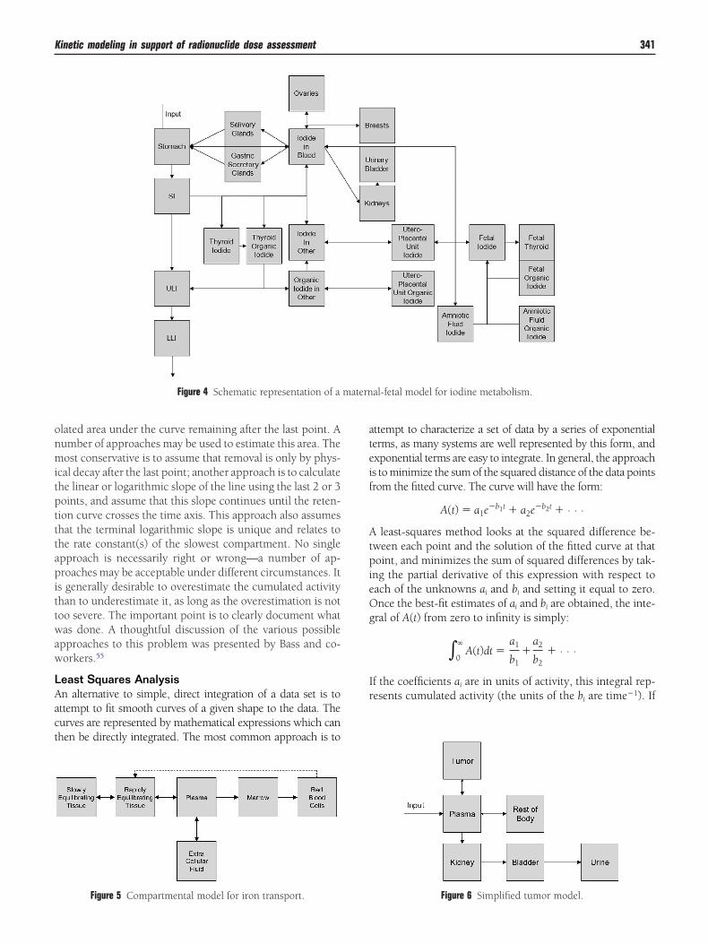
4. The need for estimates of radiation dose to the motherand fetus from large environmental releases of radioac-tive iodine (Chernobyl accident), led Berkovski andICRP49 to promulgate a more complex model (Fig. 4).Default values for many rates were chosen based onexpected normal values.
5. Iron kinetics processes and dosimetry in patients in aMIRD publication in which a single model was used torepresent iron transport in normal and altered diseasestates (Fig. 5).50 See reference for rate constants forpatients in different disease states.
6. Given interest in tumor dosimetry, a simplified model(Fig. 6), has been adapted from ICRU 67.51
Computer software has been of paramount importance inllowing the accurate numerical solution of physiologicallyealistic models and, at the same time, providing computa-
Figure 3 Schematic representation of a compartmental mformed in the urine, plasma iodide, T3, and T4 compartm
igure 2 Schematic representation of a biokinetic model for oralntake of iodide.
also measured.
ional and statistical tools to fit such models to observations.he SAAM software has arguably been one of the first contri-utions in this area. In fact, the original motivation for theAAM codes was provided by dosimetry studies. The originalAAM codes are still available using both the original com-and line interface52 and a Windows-based interface termedinSAAM.53 In addition, a completely reengineered pro-
ram allowing for solution and fitting of nonlinear compart-ental models is available and is called the SAAM IIroject.54 Such software programs, among others, have al-
owed the modeling scientists to perform the rapid and accu-ate calculation of amounts and rates of change in variousocations of generally defined multicompartmental models.t the same time, such modeling software provides general-se tools to enforce conservation of mass and radioactivitynd evaluate the total amount of radioactivity in groups ofompartments and thus peripheral tissues of interest, eg, byumming over multiple compartmental amounts. We williscuss the methodology behind these and other tools in theemainder of this document.
imple Numerical Toolssed in Routine Practice
t can be argued that the simplest measure of absorbed doseelates to the integrals from zero to infinity of the time-activ-ty curves of a given data set. When researchers obtain pre-linical or clinical data, a number of simple tools and meth-ds are often used to obtain those integrals.
irect Integrationne can directly integrate under the actual measured valuesy a number of methods. This does not give very much in-ormation about the underlying system, but it does allow oneo calculate the number of disintegrations rather easily. Theost common method used is the Trapezoidal Method, sim-ly approximating the area by a series of trapezoids. An im-ortant concern with this method is the calculation of the
ntegrated area under the curve after the last datum. If activitys clearing slowly near the end of the data set, a significantortion of the total decays may be represented by the extrap-
for thyroid iodine metabolism. Measurements are per-in addition, aggregates of the thyroid compartments are
odelents;
onmitptttapittwaw
LAact
ateif
AtpieOg
Ir
matern
Kinetic modeling in support of radionuclide dose assessment 341
lated area under the curve remaining after the last point. Aumber of approaches may be used to estimate this area. Theost conservative is to assume that removal is only by phys-
cal decay after the last point; another approach is to calculatehe linear or logarithmic slope of the line using the last 2 or 3oints, and assume that this slope continues until the reten-ion curve crosses the time axis. This approach also assumeshat the terminal logarithmic slope is unique and relates tohe rate constant(s) of the slowest compartment. No singlepproach is necessarily right or wrong—a number of ap-roaches may be acceptable under different circumstances. It
s generally desirable to overestimate the cumulated activityhan to underestimate it, as long as the overestimation is notoo severe. The important point is to clearly document whatas done. A thoughtful discussion of the various possible
pproaches to this problem was presented by Bass and co-orkers.55
east Squares Analysisn alternative to simple, direct integration of a data set is tottempt to fit smooth curves of a given shape to the data. Theurves are represented by mathematical expressions which canhen be directly integrated. The most common approach is to
Figure 4 Schematic representation of a
Figure 5 Compartmental model for iron transport.
ttempt to characterize a set of data by a series of exponentialerms, as many systems are well represented by this form, andxponential terms are easy to integrate. In general, the approachs to minimize the sum of the squared distance of the data pointsrom the fitted curve. The curve will have the form:
A(t) � a1e�b1t � a2e�b2t � · · ·
least-squares method looks at the squared difference be-ween each point and the solution of the fitted curve at thatoint, and minimizes the sum of squared differences by tak-
ng the partial derivative of this expression with respect toach of the unknowns ai and bi and setting it equal to zero.nce the best-fit estimates of ai and bi are obtained, the inte-
ral of A(t) from zero to infinity is simply:
�0
�A(t)dt �
a1
b1�
a2
b2� · · ·
f the coefficients ai are in units of activity, this integral rep-esents cumulated activity (the units of the bi are time�1). If
al-fetal model for iodine metabolism.
Figure 6 Simplified tumor model.
tt(hid
MTvtesimtioeaodmpe
bpswtpt(strdOwEtdtTmoaftbte
rsn
mresabo
sosademtdmiecpaaa
tmpnwmsbarccsip
SMRAdpmtfhnts
342 P. Vicini et al
he coefficients give fractions of the administered activity,hen the area represents the normalized cumulated activityeg, Bq-h/Bq). Many computational kinetic modeling toolsave been developed that are in principle useful for comput-
ng pharmacokinetic parameters for calculating absorbedose in different tissues.56
ore Complex Computational Toolshe main limitation of the approach we have described pre-iously is, as we have mentioned, that no additional informa-ion is obtained about the system behavior except for infer-nce directly based on the observations. This may beufficient when only an estimate of radiation dose to organsn the body is desired. Under these circumstances, the use of
athematical models that summarize what is known abouthe system behavior can be useful to infer the biodistributionn inaccessible sites exclusively from information available inbservable sampling sites. Such inference is an aspect of thengineering inverse problem,57 and the robustness and reli-bility of predictions made in such sites can be tested basedn statistical and system identification methods and proce-ures. Others have discussed in detail structural aspects ofodel identifiability and whether inference on remote com-artments can be well posed, conditional on limited knowl-dge on accessible sites.58
Least squares, and especially weighted least squares, haveeen for many years the tool of choice for fitting multicom-artmental models to data.59 The advantage of weighted leastquares is to provide a straightforward and formally accurateay to explicitly incorporate the knowledge (when available)
hat data points collected over time may be more or lessrecise. Knowledge of the measurement error then shapeshe relative importance of the contribution of every residualdifference between model and data) to the overall weightedum of squares. In addition, the statistical interpretation ofhe data weights (proportional to the data measurement er-or) allows for the accurate calculation of parameter confi-ence intervals, now available in many modeling packages.ther least squares approaches relax the assumption that theeights are calculated conditional on the measured value.xtended least squares approaches60 have also a natural in-
erpretation based on maximum likelihood, and use the pre-icted value, as opposed to the measured value, to calculatehe weight for each residual in the weighted sum of squares.his minimizes the impact of noisy and scattered measure-ents on the calculation of the weights, and smoothes the
verall weighting scheme. Extended least squares methodsre also available in several modeling packages. Clearly, dif-ering assumptions about the data weights have the potentialo return different parameter estimates.61,62 Thus, inferenceased on data are always conditional not only on the shape ofhe curve, but also on the measurement error associated withvery data point on the curve.
Another factor that is relevant to the performance of pa-ameter estimation methods is the temporal location of theamples, together with their number. Loosely speaking, the
umber of samples is related to the number of compart- yents, or separate exponential terms, while their timing iselated to the exponentials’ decay rates. Rapidly decayingxponentials, for example, will necessitate frequent and earlyampling, while slowly decaying exponentials require fewernd more widely spaced measurements. These topics haveeen studied extensively elsewhere, in quantitative physiol-gy,59 pharmacokinetics63 and nuclear medicine.51,64
Population estimates of model rate constants and expo-ures can be constructed by aggregating individual estimatesbtained by repeated experiments in a number of individualubjects. Such aggregation can be performed by calculatingrithmetic means or medians, depending on the underlyingistribution and the availability of individual data. Individualstimates must be available for this method to work. Another,ore recent class of methods that has found extensive applica-
ion in pharmacokinetics, but not as much so far in radiationosimetry, is the family of approximate maximum likelihoodethods which is usually termed “population pharmacokinet-
cs.”65 This is a class of nonlinear mixed effects models thatxplicitly represents, in addition to the functional form of theurve to be modeled, the probability distribution of its modelarameters in the population of interest. Such an approachllows estimating population features with reasonable reli-bility, even when individual estimates are not available, orre extremely imprecise.66
The model building process uses the parameter estimationools that we have described to narrow the model space to theost parsimonious, but robust, structure that the data sup-ort. This may start with a preliminary investigation of theumber of exponentials in the system (for linear systems),hich would dictate the number of compartments for initialodel exploration. For systems which do not behave like
ums of exponentials, numerical integration techniques maye employed to model the sample sites. Competing modelsre then tested on the basis of the reduction in measurementesidual variance that they provide, in addition to parsimonyriteria that penalize more complex models in favor of lessomplex ones. Against this background, physiological plau-ibility must always be taken into account, and a physiolog-cally plausible model should be considered superior to aarsimonious, but oversimplified, one.
pecial Kineticodels Developed foradioisotope Dosimetry Analysesnumber of kinetic models have been developed to facilitate
ose calculations in several special cases. Often, models haverogressed from simple to complex or from less detailed toore detailed, depending on the specific application and
heir intended use. An example of this is the Berkovski modelor iodine kinetics for pregnant women and children whoad accidentally been exposed to radiation from the Cher-obyl accident and how it incorporates parameters and struc-ures from the basic Berman model. Below we describe aeries of example models that have been developed over the
ears for some general applications.
USbbttotaqtpeteia
(elsb
pibithbptch0
0dttemittc
GIrdvqtIIdtTtswttIsmtmk
Fio
Fd
Kinetic modeling in support of radionuclide dose assessment 343
rinary Bladderhort-lived radionuclide labeled small molecules are filteredy the glomerulus and rapidly excreted; thus, kidney andladder modeling is important to describe the kinetics ofhese substances. When activity is excreted from the body inhe urine, the function that describes it usually consists of oner more exponential terms. Fitting observed activity levels inhe urinary bladder is not helpful, because the bladder fillsnd empties repeatedly, and measurements are too infre-uently gathered to characterize this time-activity curve. Ma-erial leaving the body is most often governed by first orderrocesses, which mean that the retention (in the body) can bexpressed as a function such as A · exp(�� t). Therefore, theime-activity curve for the bladder takes the form of A · (1 �xp(�� t)), but the curve is periodically interrupted by void-ng and goes to zero (or nearly zero) and then begins toccumulate again, as in Figure 7.
What is needed is a characterization of the values A and �in real situations there may be more than one term in thequation, but for now, let’s just consider one). In a particu-arly ingenious derivation, Walt Snyder and colleagues67
howed that the number of disintegrations occurring in theladder could be given in such cases by a single equation:
N � A0�i
fi�1 � e��iT
�i�
1 � e�(�i��p)T
�i � �p�� 1
1 � e�(�i��p)T�Here, A0 is the initial activity entering the body, �p is the
hysical decay constant of the radionuclide, �i is the biolog-cal removal constant for the fraction of activity fi leaving theody via the urinary pathway, and T is the bladder voiding
nterval, assumed to be constant. If we have all the activity inhe body passing out through the urinary pathway with a 1our half-time, for example, our f would be 1.0 and � woulde 0.693/1 hour � 0.693 hour�1. Let’s say we have 40%assing out through the gastrointestinal (GI) tract, and 60%hrough the urinary pathway, with two-thirds of the urinarylearance having a half-time of 1 hour and one-third with aalf-time of 10 hours. Then f1 would be 0.4 and �b1 would be.693 hour�1, and f2 would also be 0.2 and �b2 would be
igure 7 The influence of urinary bladder voiding schedule is shownn comparison with the urinary accumulation curve in the absence
tf voiding. (Color version of figure is available online.)
.0693 hour�1. These parameters are not particularly hard toerive - one must either measure the total body retention orhe cumulative urinary excretion and fit a function, either ofhe form A · exp(�� t) (in the former case) or A · (1 �xp(�� t)) (in the latter case). Again, the equation may haveore than one term, depending on the data observed. If there
s GI excretion, this complicates the use of whole body reten-ion data, unless intestinal activity is somehow excluded fromhe images. But in either case, the complication can be over-ome by careful data gathering and inspection of the results.
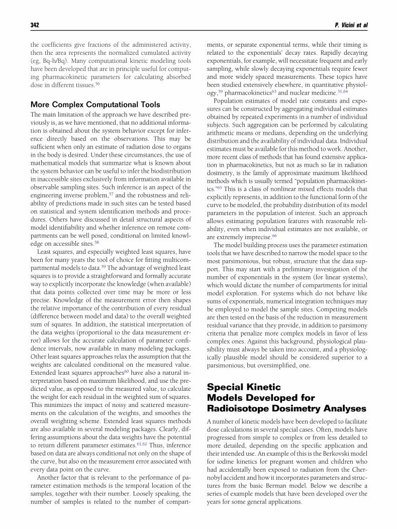
astrointestinal Tractngestion is a common means of intake of radioactive mate-ial, either through swallowing of material somehow intro-uced into the mouth or through transfer of material from thearious regions of the lung system to the throat and subse-uent swallowing. A standardized kinetic model of the GIract was first proposed by Eve68 and was adopted by thenternational Commission on Radiological Protection inCRP Publication 30.69 Four sections of the GI tract wereefined (Fig. 8), having separate kinetics, with activity inhe contents passing through with standard rate constants.he walls of the various sections and were treated as separate
arget tissues according to the ICRP 30 (Fig. 8) dosimetricystem. At that time, they were not assigned any specificeighting factors for calculation of “effective dose” quanti-
ies, and were treated, if significant, as ‘remainder’ tissues inhis calculation. In more recent recommendations of theCRP, however, segments of the GI tract have been assignedpecific risk weighting factors. A more detailed and realisticodel has been recommended recently by the ICRP, named
he Human Alimentary Tract (HAT) model (Fig. 9). Thisodel has more compartments, includes some nonfirst order
inetic components, models age-dependent compartment
igure 8 The components defining the pathways influencing theose to the GI tract in the ICRP 30 model.69
ransfer rates, treats liquid and solid materials differently, and
cs
BBhovnhirobdme(tibcbltrt
bcuiod
cti
wirsap
mvtd
CImetbptddtbpbaupfbfetd
R
FdI
344 P. Vicini et al
alculates doses to segments of the HAT not previously con-idered.70
one Marrowone marrow is a highly radiosensitive, rapidly turning overematopoietic organ. The red marrow is distributed through-ut the different regions of the skeleton in a fashion thataries with age.71 When increased uptake of radioactivity isoted in bone marrow-containing regions, different methodsave been used to separate the marrow content from super-
mposed activity in the surrounding bone, adjacent and sur-ounding blood vessels.72,73 Given the number and locationf vertebrae sampled, one then estimates the fraction of totalone marrow contained in those sites based on reference manistribution values.71 The need for bone marrow dose esti-ates derives from interest in estimating risk of stochastic
ffects (diagnostic exposures) and of deterministic effectstherapeutic exposures). These measures are also importanto the physician in planning and evaluating effects of admin-stered therapy. When the tumor-involved marrow site haseen invaded by tumor, the dose to these measured regionsonveys a desired effect. Lower concentrations of activity inlood which circulates through uninvolved regions convey a
ower dose to normal marrow. Given an estimate of the frac-ion of marrow that is occupied by tumor, the dose to thoseegions is estimated directly from the measured uptake and
igure 9 The components defining the pathways influencing theose to the different segments of the GI tract are defined in the newCRP Human Alimentary Tract Model (HAT) model.70
he dose to the remaining fraction of the marrow is based on
lood contributions. Compartment models can be used toompute marrow dose weighting these two contributionssing the modeling tools described earlier, in particular by
nterrogating and then summing over time the contributionsf several compartments in the model, even those that are notirectly amenable to measurement.When uptake is not visualized in the marrow, the most
ommonly-used method measures the amount of activity inhe blood as a function of time, and assumes that the uptaken marrow can be related to the activity in blood:
[Amarrow] � [Ablood] � RMBLR
here [Amarrow] is the concentration of compound (assumedn this publication to be a monoclonal antibody) in the mar-ow, [Ablood] is the concentration of the agent in the blood orerum, and RMBLR is the red marrow to blood cumulatedctivity ratio. One expression of this, used by many was pro-osed by Sgouros74:
[Amarrow] � [Ablood]RMECFF
(1 � HCT)
Here, RMECFF is the vascular and ECF volume in thearrow, and HCT is the patient hematocrit. The “working”
alue for the RMECFF was suggested to be 0.19. Other au-hors75 have adapted this method to other agents, assumingifferent values for the RMECFF.
onclusionsn this short, and by necessity incomplete, review of mathe-atical models that have been used or can be used in dosim-
try applications we have attempted to cover ground both onhe methodology and the applications. We have tried toriefly review the origins of existing methodology for com-artmental modeling and parameter estimation, at the sameime attempting to review other, more recent methodologicalevelopments that could be useful in future applications ofosimetry. We have also listed example models and calcula-ions, so as to provide the reader with an overview of thereadth of kinetic model applications in dosimetry. It isrobably worthwhile to remind the reader that the modeluilding process is only in part facilitated by the ready avail-bility of large computational power and accurate and easy tose modeling software. By and large, the definition and ap-lication of these models remains, to a large extent, an artorm, whose practitioners remain few and far between. Theackground of these scientists spans a tremendous range,rom physics to biology, and engineering and computer sci-nce. The variety of model applications we have listed andhe impact these models continue to have on the practice ofosimetry gives testimony to their creativity and ingenuity.
eferences1. ICRP: International Commission on Radiological Protection: History,
Policies, Procedures. Oxford, Elsevier Science Ltd, 19982. Luigi Bertelli (Vamba): Il Giornalino di Gian Burrasca. Firenze, Bem-
porad, 1912
1
1
1
1
1
1
1
1
1
1
2
2
2
2
2
2
2
2
2
2
3
3
3
3
3
3
3
3
3
3
4
4
4
4
4
4
4
4
4
4
5
5
5
5
5
5
5
5
Kinetic modeling in support of radionuclide dose assessment 345
3. Chievitz O, Hevesy G: The first radioindicator study in the life scienceswith a man-made radionuclide. Nature 1935;136:754-755. Reprintedin J Nucl Med 16:1107-1108, 1976 [Commentary by W.G. Myers]
4. Cobelli C, Foster D, Toffolo G: Tracer Kinetics in Biomedical Research:From Data to Model. San Diego, Kluwer Academic/Plenum Publishers,2000
5. Rowland M, Balant L, Peck C: Physiologically based pharmacokineticsin drug development and regulatory science: A workshop report(Georgetown University, Washington, DC, May 29-30, 2002). AAPSPharm Sci 6:E6, 2004
6. Stabin MG, Brill AB: State of the art in nuclear medicine dose assess-ment. Semin Nucl Med 38:308-320, 2008
7. Berman M: Kinetic models for absorbed dose calculations. MIRD Pam-phlet No. 12, Society of Nuclear Medicine, Jan. 1977
8. Akaike H: A new look at the statistical model identification. IEEE TransAutomatic Control 19:716-723, 1974
9. Schwarz G: Estimating the dimension of a model. Ann Stat 6:461-464,1978
0. Rescigno A: The rise and fall of compartmental analysis. Pharmacol Res44:337-342, 2001
1. Becquerel H: Sur les radiations émises par phosphorescence. ComptesRendus de l’Académie des Sciences (Paris) 122:420-421, 1896
2. Becquerel H: Sur les Radiations Invisibles Émises par les Corps Phos-phorescents. Comptes Rendus Acad Scis (Paris) 122:501-503, 1896
3. Rutherford E, Soddy BA: The cause and nature of radioactivity. Philo-sophical Magazine 4:370, 1902
4. Rutherford E: The succession of changes in radioactive bodies. R SocLond Phil Trans 204:169, 1904
5. Behnke AR, Thomson RM, Shaw LA: The rate of elimination of dis-solved nitrogen in man in relation to the fat and water content of thebody. Am J Physiol 114:137-146, 1935
6. Teorell T: Kinetics of distribution of substances administered to thebody. I: The extravascular modes of administration. Arch Int Pharma-codyn Thér 57:205-225, 1937
7. Teorell T: Kinetics of distribution of substances sdministered to thebody. II: The Intravascular Modes of Administration. Arch Int Pharma-codyn Thér 57:226-240, 1937
8. DiStefano JJ 3rd, Landaw EM: Multiexponential, multicompartmental,and noncompartmental modeling. I: Methodological limitations andphysiological interpretations. Am J Physiol 246:R651-R664, 1984
9. Artom C, Sarzana G, Segré E: Influence des grasses alimentaires sur laformation des phospholipides dans les tissues animaux (nouvelles re-cherches). Arch Int Physiol 47:245-276, 1938
0. Goresky CA: A linear method for determining liver sinusoidal andextravascular volumes. Am J Physiol 204:626-640, 1963
1. Sheppard CW: The theory of the study of transfers within a multi-compartment system using isotopic tracers. J Appl Phys 19:70-76,1948
2. Sheppard CW, Householder AS: The mathematical basis of the inter-pretation of tracer experiments in closed steady-state systems. J ApplPhys 22:510-520, 1951
3. Rescigno A, Segre G: La Cinetica dei Farmaci e dei Traccianti Radioat-tivi. Torino, Boringhieri, 1961
4. Hearon JZ: Theorems on Linear Systems. Ann N Y Acad Sci 108:36-68,1963
5. Brownell GL, Berman M, Robertson JS: Nomenclature for tracer kinet-ics. Int J Appl Rad Isot 19:249-262, 1968
6. Berman M: Iodine kinetics. Methods of investigative and diagnosticendocrinology. Amsterdam, North-Holland Publishing Co., 1972
7. Rescigno A, Beck JS: Compartments, in Rosen R (ed): Foundations ofMathematical Biology. Volume 2. New York, Academic Press, 1972, pp255-322
8. Jacquez JA: Compartmental Analysis in Biology and Medicine. Amster-dan, Elsevier, 1972
9. Gurpide E: Tracer Methods in Hormone Research. New York, Springer-Verlag, 1975
0. Siri W: Isotopic tracers and nuclear radiations with applications tobiology and medicine, in Theory of Tracer Methods. New York,
McGraw-Hill, 19491. Schmidt KC, Turkheimer FE: Kinetic modeling in positron emissiontomography. Q J Nucl Med 46:70-85, 2002
2. Bertoldo A, Vicini P, Sambuceti G, et al: Evaluation of compartmentaland spectral analysis models of [18F]FDG kinetics for heart and brainstudies with PET. IEEE Trans Biomed Eng 45:1429-1448, 1998
3. Rescigno A, Beck JS: Compartments, in Rosen R (ed): Foundations ofMathematical Biology, Volume II: Cellular Systems. New York, Aca-demic Press, pp 255-322, 1972
4. Bergner PEE: The significance of certain kinetic methods, especiallywith respect to the tracer dynamic definition of metabolic turnover.Acta Radiol Suppl 210:1-59, 1962
5. Zierler K: A critique of compartmental analysis. Ann Rev Biophys Bio-eng 10:531-562, 1981
6. Rescigno A, Beck JS: The use and abuse of models. J PharmacokinBiopharm 15:327-340, 1987
7. Rescigno A: On the use of pharmacokinetic models. Phys Med Biol49:4657-4676, 2004
8. Rescigno A: Clearance, turnover time, and volume of distribution.Pharmacol Res 35:189-193, 1997
9. Robertson JS: Theory and use of tracers in determining transfer rates inbiological systems. Physiol Rev 37:133-154, 1957
0. Berman M: Iodine kinetics in man—a model. J Clin Endocrin Metab28:1-14, 1968
1. Berkovski V, Eckerman KF, Phipps AW, et al: Dosimetry of radioiodinefor embryo and fetus. Radiat Prot Dosimetry 105:265-268, 2003
2. Berman M: The formulation and testing of models. Ann NY Acad Sci108:182-194, 1963
3. Berman M, Weiss MF, Shahn E: Some formal approaches to the analysisof kinetic data in terms of linear compartment systems. Biophys J2:289-316, 1962
4. Berman M, Schoenfeld R: Invariants in experimental data on linearkinetics and the formulation of models. J Appl Phys 27:1361-1370,1956
5. DiStefano JJ 3rd: Noncompartmental vs. compartmental analysis: Somebases for choice. Am J Physiol 243:R1-R6, 1982
6. DiStefano JJ 3rd: Concepts, properties, measurements, and computa-tion of clearance rates of hormones and other substances in biologicalsystems. Ann Biomed Eng 4:302-319, 1976
7. Oddie TH: Analysis of radio-iodine uptake and excretion curves. Br JRadiol 257:261-267, 1949
8. Johansson L, Leide-Svegborn S, Mattsson S, et al: Biokinetics of iodidein man: Refinement of current ICRP dosimetry models. Cancer BiotherRadiopharma 18:445-450, 2003
9. Berkovski V: New iodine models family for simulation of short-termbiokinetics processes, pregnancy and lactation. Food Nutr Bull 23:87-94, 2002 (suppl)
0. Robertson JS, Price RR, Budinger TF, et al: MIRD Report No. 11. Iron-52, Fe-55, and Iron-59 used to study ferrokinetics. J Nucl Med 24:339-348, 1983
1. International Commission on Radiation Units and Measurements(ICRU): Absorbed-Dose Specification in Nuclear Medicine. ICRU-Re-port 67. Bethesda, MD, ICRU, 2002
2. Boston RC, Greif PC, Berman M: Conversational SAAM—an interactiveprogram for kinetic analysis of biological systems. Comput ProgramsBiomed 13:111-119, 1981
3. Greif P, Wastney M, Linares O, et al: Balancing needs, efficiency, andfunctionality in the provision of modeling software: A perspective of theNIH WinSAAM Project. Adv Exp Med Biol 445:3-20, 1998
4. Barrett PH, Bell BM, Cobelli C, et al: SAAM II: Simulation, analysis, andmodeling software for tracer and pharmacokinetic studies. Metabolism47:484-492, 1998
5. Bass L, Aisbett J, Bracken AJ: Asymptotic forms of tracer clearancecurves: Theory and applications of improved extrapolations. J TheoretBiol 111:755-785, 1984
6. Pharmakinetic software. Available at: http://www.boomer.org/pkin/soft.html. Accessed May 21, 2008
7. Cobelli C, Caumo A: Using what is accessible to measure that which is
not: Necessity of model of system. Metabolism 47:1009-1035, 1998
5
5
6
6
6
6
6
6
6
6
6
6
7
7
7
7
7
7
346 P. Vicini et al
8. Cobelli C, DiStefano JJ 3rd: Parameter and structural identifiabilityconcepts and ambiguities: A critical review and analysis. Am J Physiol239:R7-R24, 1980
9. Landaw EM, DiStefano JJ 3rd: Multiexponential, multicompartmental,and noncompartmental modeling. II: Data analysis and statistical con-siderations. Am J Physiol 246:R665-R677, 1984
0. Sheiner LB, Beal SL: Pharmacokinetic parameter estimates from severalleast squares procedures: Superiority of extended least squares. J Phar-macokin Biopharm 13:185-201, 1985
1. Spilker ME, Vicini P: An evaluation of extended vs weighted leastsquares for parameter estimation in physiological modeling. J BiomedInform 34:348-364, 2001
2. Muzic RF, Jr., Christian BT: Evaluation of objective functions for esti-mation of kinetic parameters. Med Phys 33:342-353, 2006
3. D’Argenio DZ: Optimal sampling times for pharmacokinetic experi-ments. J Pharmacokin Biopharm 9:739-756, 1981
4. Siegel JA, Thomas SR, Stubbs JB, et al: MIRD pamphlet no. 16: Tech-niques for quantitative radiopharmaceutical biodistribution data acqui-sition and analysis for use in human radiation dose estimates. J NuclMed 40: 37S-61S, 1999
5. Beal SL, Sheiner LB: Estimating population kinetics. Crit Rev BiomedEng 8:195-222, 1982
6. Sheiner LB, Beal SL: Evaluation of methods for estimating population
pharmacokinetic parameters. III: Monoexponential model: Routineclinical pharmacokinetic data J Pharmacokin Biopharm 11:303-319,1983
7. Cloutier R, Smith S, Watson E, et al: Dose to the fetus from radionu-clides in the bladder. Health Phys 25:147-161, 1973
8. Eve IS: A review of the physiology of the gastrointestinal tract in relation toradiation doses from radioactive material. Health Phys 12:131-161, 1966
9. International Commission on Radiological Protection: Limits for In-takes of Radionuclides by Workers. ICRP Publication 30. New York,Pergamon Press, 1979
0. ICRP Publication 100 Human Alimentary Tract Model for RadiologicalProtection. Volume 35, Issue 4. ICRP Press, 2005, pp 1-142
1. ICRP Publication 89: Basic Anatomical And Physiological Data for Usein Radiological Protection: Reference Values, ICRP Press, 2003
2. Stabin MG, Eckerman KF, Bolch WE, et al: Evolution and status of boneand marrow dose models. Cancer Biother Radiopharm 17:427-434,2002
3. Sgouros G, Stabin M, Erdi Y, et al: Red marrow dosimetry for radiola-beled antibodies that bind to marrow, bone or blood components. MedPhys 27:2150-2164, 2000
4. Sgouros G: Bone marrow dosimetry for radioimmunotherapy; Theoret-ical consideration. J Nucl Med 34:689-694, 1993
5. Cremonesi M, Ferrari M, Bodei L, et al: Dosimetry in peptide radionu-
clide receptor therapy: A review. J Nucl Med 47:1467-1475, 2006