Embed Size (px)
Citation preview
Applied Geochemistry 53 (2015) 13–26
Contents lists available at ScienceDirect
Applied Geochemistry
journal homepage: www.elsevier .com/ locate/apgeochem
Kinetic modeling of interactions between iron, clay and water:Comparison with data from batch experiments
http://dx.doi.org/10.1016/j.apgeochem.2014.12.0030883-2927/� 2014 Elsevier Ltd. All rights reserved.
⇑ Corresponding author. Tel.: +33 (0)368 850 472.E-mail addresses: [email protected], [email protected] (V.V. Ngo).
Viet V. Ngo a,⇑, Alain Clément a, Nicolas Michau b, Bertrand Fritz a
a Laboratoire d’Hydrologie et de Géochimie de Strasbourg, Université de Strasbourg/EOST, CNRS, 1 rue Blessig, F-67084 Strasbourg Cedex, Franceb Andra, Parc de la Croix Blanche, 1/7 rue Jean Monnet, F-92298 Châtenay-Malabry Cedex, France
a r t i c l e i n f o
Article history:Available online 9 December 2014Editorial handling by M. Kersten
a b s t r a c t
It has been proposed that a carbon steel overpack is used as part of the engineered barrier system for thegeological disposal of radioactive wastes developed by Andra. The direct contact of the iron with the geo-logical environment creates potential physical and chemical changes in the near field environment of therepository. Therefore, a thorough understanding of the mineralogical/chemical evolution caused by theinteractions of iron with clay is necessary to the assessment of the performance of the geological disposal.Geochemical models have been developed (using the code KINDIS) to simulate batch experiments oniron–claystone interactions. The experiments included iron power and Callovo-Oxfordian (COx) claystonethat were reacted at temperature of 90 �C for 90 days. The overall objective of this modeling work aims atan enhanced mechanistic understanding of clay–iron interactions observed in experimental studies andpossible implications for engineered barrier performance.
The experimental observations were successfully reproduced by the model regarding geochemical evo-lution and mineralogical transformations. For example, the stability of pH around 7 and total dissolvedcarbon in the aqueous solution, which are controlled by saturation state of carbonates in the system,are predicted accurately. In addition, the model predicts that during the interactions between iron andclays greenalite, chukanovite, and saponite form as the main secondary minerals. Moreover, the destabi-lization of some important primary minerals in the claystone such as quartz, illite, and smectite are alsoindicated by the numerical simulations. The consistency of the predictions with the experimental obser-vations can be shown in activity diagrams of these secondary minerals, which represent the relation ofH4SiO4 activity and CO2 partial pressure or Ca2+ activity. Another important result is that both the modeland experimental data indicated that magnetite is not formed in the experiments.
The analysis of three sensitivity cases made clear that the uncertainty in corrosion and dissolution ratesfor iron, quartz, and illite plays an important role on the predicted evolution of pH in the aqueous solutionand the formation of secondary minerals. Through this modeling work, the controlling mechanism of theinteractions of iron, clay, and water at the specific conditions is fairly well understood. However, therobustness of the geochemical code KINDIS should also be tested against other experiments with differ-ent experimental conditions.
� 2014 Elsevier Ltd. All rights reserved.
1. Introduction
The concept of deep geological repository developed by Andragenerally consists of using the remarkable physical and chemicalproperties of the claystone (e.g., retention capability, low perme-ability, and homogeneity of the formation). The claystone hasproperties that are desirable for a host rock for radioactive wastedisposal, in that it has low water flow, and radionuclide migrationcan only occur via very slow diffusion processes. The COx claystonefrom the Paris basin can satisfy all the above properties and hence
these are investigated in various studies. Additionally, in Andra’sdesign, the confinement of high level radioactive waste requiresa steel canister to avoid any release of the radioactive species forat least a few centuries. The direct contact between the steel can-ister and the geological barrier creates potential issues related tothe iron corrosion that causes the mineralogical transformationsin the near field environment. It is expected that during corrosionof the steel overpack, iron reacts with water, clay minerals, silicatesand carbonates of the claystone to form corrosion products like:magnetite, dihydrogen, iron silicates and iron carbonates. Exten-sion of this transformed zone and its chemical composition mayinfluence the behavior and the transfer of radionuclides on thelong term. Therefore, an understanding of the evolution of the
14 V.V. Ngo et al. / Applied Geochemistry 53 (2015) 13–26
environment in the repository over long periods of time is essentialfor the performance assessment of the geological disposal.
Considerable attention has been paid to this system through theexperimental investigations of the interactions between iron andclay host rock and/or bentonite using different approaches thattry to represent different repository conditions. Such studiesinclude the in situ field experiments (e.g., Gaudin et al., 2009,2013) and the laboratory experiments (e.g., Guillaume et al.,2003, 2004; Jodin-Caumon et al., 2010, 2012; Lantenois et al.,2005; Martin et al., 2008; Mosser-Ruck et al., 2010; Perronnetet al., 2007; Rivard et al., 2013a,b; Schlegel et al., 2008, 2010;Wilson et al., 2006a; Lanson et al., 2012). Depending on the exper-imental conditions, mineralogical compositions, aqueous chemis-try, and the physical chemical parameters such as pH, Eh, andtemperature, the reaction pathways and evolution of the experi-mental systems are significantly different. A number of differentalteration products have been observed, including Fe-rich clayminerals, zeolites and iron oxides. (Mosser-Ruck et al., 2010). Nev-ertheless, it is commonly found from these publications that theinteractions between iron and clays can form magnetite and Fe-rich silicates as the main corrosion products. Moreover, some ofthe above experimental investigations have also reported thedestabilization of quartz, illite, and smectite (e.g., de Combarieuet al., 2007; Mosser-Ruck et al., 2010; Perronnet et al., 2007).Recent technical developments, like electron diffraction tomogra-phy, X-ray absorption spectroscopy or scanning transmissionX-ray microscopy, allow very fine characterization of the mineral-ogical transformations of the aqueous and solid phases (e.g., Rivardet al., 2013a,b; Schlegel et al., 2008, 2010; Jodin-Caumon et al.,2010; Pignatelli et al., 2013; Wilson et al., 2006a).
In the literature, there are, however, limited modeling studiesabout the interactions between iron and clay materials (Bildsteinet al., 2006; de Combarieu et al., 2007; Montes-H et al., 2005;Savage et al., 2010; Wilson et al., 2006b). Up to date, to our knowl-edge, there is even only one published modeling study undertakenby de Combarieu et al. (2007) about the interactions involving COxclaystone and iron at the laboratory scale. Therefore, additionalstudies about this aspect would be useful since a thorough under-standing of potential evolution and mechanism of the interactionsbetween such materials via the modeling tools is crucial to under-pin the Andra concept of radioactive waste confinement.
Kinetic modeling requires a dissolution equation for each pri-mary mineral. The dissolution of primary minerals is one of themost important processes that control the evolution of the systemwhen investigating the interactions of clay and water. The dissolu-tion rate of a mineral depends on many factors. These include thetemperature of the system, the surface area available for dissolu-tion, the solution composition (in particular pH), and the deviationfrom reaction equilibrium. Several formulations with respect to themineral dissolution and precipitation have been proposed in theliterature (e.g., Arvidson and Luttge, 2010; Beig and Lüttge, 2006;Burch et al., 1993; Lasaga et al., 1994). The formulation developedby Lasaga et al. (1994) is widely applied and is expressed asfollows:
rd ¼ kde�Ea=RT SigðIÞY
a
anii f ðDGÞ ð1Þ
where kd is the dissolution rate constant, Si is the reactive surfacearea of mineral i, Ea and DG are the apparent activation energyand the Gibbs free energy of the overall reaction, ai and ni are theactivity of the ith species involved in the reaction mechanism andthe reaction order with respect to this species, g(I) is a function ofionic strength, f(DG) is a function of the Gibbs free energy.
The formulation of the function f(DG) is generally based on theTransition State Theory (TST), which allows to express it by the lin-ear relationship, f ðDGÞ ¼ 1� exp DG
RT
� �� �. Depending on the types of
minerals and experimental conditions, the dissolution mechanismis more or less complex and may be very different. There is still adebate in the scientific community about the form of functionf(DG) (e.g., Arvidson and Luttge, 2010; Daval et al., 2010;Hellmann and Tisserand, 2006; Schott et al., 2009, 2012). Someauthors accept that there is a linear relationship between the min-eral dissolution rate and DG while the others consider that it mustbe a non-linear dependence between them, especially at near equi-librium conditions.
The geochemical modeling tools being currently developed inour laboratory implement the rate law of mineral dissolution basedon the TST. It is, thus, essential to assess their performance inreproducing dissolution–precipitation experiments. For this practi-cal application with respect to the interactions of COx claystoneand iron, we face some issues related to a large mineralogical var-iability of the clays used in the model and the difficulties in param-eterization of kinetic data of a dozen of primary minerals.Therefore, the objective of the current study is not to attempt toreproduce exactly the experimental data, but aims at an enhancedmechanistic understanding of reaction pathways and controllingparameters for interactions of iron, COx claystone, and water inthe given experimental conditions.
2. Materials and methods
2.1. Overview of the experiments
In the context of the geological disposal for high level radioac-tive waste, Andra has been supporting different studies about theinteractions of iron, clays, and water. The experiments modeledin this work were carried out by the team of the GéoRessourceslaboratory (Bourdelle et al., 2014), University of Lorraine. The batchexperiments were performed to investigate the mineralogical andchemical evolutions of the system in different conditions. Theyhave been developing equipment in which pH can be measuredin real time and in situ. Furthermore, the aqueous and solid phaseswere also sampled to analyze aqueous species and mineralogicalfractions of the solid phase during the experiment. In this modelingwork, two in situ batch experiments were selected, which had thehighest resolution and quality of data. In this section, the overalldescription of the experiments and a summary of the results aregiven. Greater detail on the experiments is provided by Bourdelleet al. (2014).
2.1.1. Experimental descriptionThe two experiments were carried out in parallel by means of
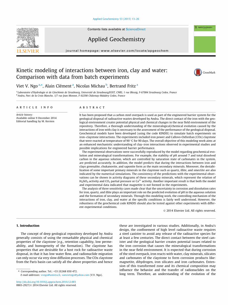
two autoclaves with a volume of 250 cm3. One autoclave was usedto measure the in situ pH evolution, called ‘‘pH experiment’’, inwhich no fluid, gas, and solid phases were sampled during theexperiment to avoid any fluctuation. At the end of this experiment,different phases were analyzed. The second autoclave was used toperform the so-called ‘‘LG experiment’’, in which the solid andaqueous phases were sampled at different successive times todetermine the evolution of the solid phase and to analyze majorions and other species. Fig. 1 shows a schematic view of theseexperiments.
The temperature of both experiments was kept constant at90 �C. It is assumed that the initial input of both experiments suchas mineralogical composition of COx claystone, iron, and aqueoussolution are the same. The experimental system contained ironand COx claystone in the form of powder with the following weightratios: water/clay = 10 and iron/clay = 0.1. The water used in bothexperiments initially contained NaCl (20.7 mM L�1) and CaCl2
(3.8 mM L�1). These experiments were carried out for a period of90 days.
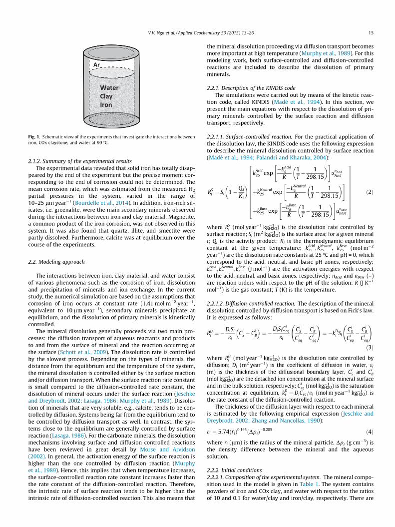
WaterClayIron
Ar
Fig. 1. Schematic view of the experiments that investigate the interactions betweeniron, COx claystone, and water at 90 �C.
V.V. Ngo et al. / Applied Geochemistry 53 (2015) 13–26 15
2.1.2. Summary of the experimental resultsThe experimental data revealed that solid iron has totally disap-
peared by the end of the experiment but the precise moment cor-responding to the end of corrosion could not be determined. Themean corrosion rate, which was estimated from the measured H2
partial pressures in the system, varied in the range of10–25 lm year�1 (Bourdelle et al., 2014). In addition, iron-rich sil-icates, i.e. greenalite, were the main secondary minerals observedduring the interactions between iron and clay material. Magnetite,a common product of the iron corrosion, was not observed in thissystem. It was also found that quartz, illite, and smectite werepartly dissolved. Furthermore, calcite was at equilibrium over thecourse of the experiments.
2.2. Modeling approach
The interactions between iron, clay material, and water consistof various phenomena such as the corrosion of iron, dissolutionand precipitation of minerals and ion exchange. In the currentstudy, the numerical simulation are based on the assumptions thatcorrosion of iron occurs at constant rate (1.41 mol m�2 year�1,equivalent to 10 lm year�1), secondary minerals precipitate atequilibrium, and the dissolution of primary minerals is kineticallycontrolled.
The mineral dissolution generally proceeds via two main pro-cesses: the diffusion transport of aqueous reactants and productsto and from the surface of mineral and the reaction occurring atthe surface (Schott et al., 2009). The dissolution rate is controlledby the slowest process. Depending on the types of minerals, thedistance from the equilibrium and the temperature of the system,the mineral dissolution is controlled either by the surface reactionand/or diffusion transport. When the surface reaction rate constantis small compared to the diffusion-controlled rate constant, thedissolution of mineral occurs under the surface reaction (Jeschkeand Dreybrodt, 2002; Lasaga, 1986; Murphy et al., 1989). Dissolu-tion of minerals that are very soluble, e.g., calcite, tends to be con-trolled by diffusion. Systems being far from the equilibrium tend tobe controlled by diffusion transport as well. In contrast, the sys-tems close to the equilibrium are generally controlled by surfacereaction (Lasaga, 1986). For the carbonate minerals, the dissolutionmechanisms involving surface and diffusion controlled reactionshave been reviewed in great detail by Morse and Arvidson(2002). In general, the activation energy of the surface reaction ishigher than the one controlled by diffusion reaction (Murphyet al., 1989). Hence, this implies that when temperature increases,the surface-controlled reaction rate constant increases faster thanthe rate constant of the diffusion-controlled reaction. Therefore,the intrinsic rate of surface reaction tends to be higher than theintrinsic rate of diffusion-controlled reaction. This also means that
the mineral dissolution proceeding via diffusion transport becomesmore important at high temperature (Murphy et al., 1989). For thismodeling work, both surface-controlled and diffusion-controlledreactions are included to describe the dissolution of primaryminerals.
2.2.1. Description of the KINDIS codeThe simulations were carried out by means of the kinetic reac-
tion code, called KINDIS (Madé et al., 1994). In this section, wepresent the main equations with respect to the dissolution of pri-mary minerals controlled by the surface reaction and diffusiontransport, respectively.
2.2.1.1. Surface-controlled reaction. For the practical application ofthe dissolution law, the KINDIS code uses the following expressionto describe the mineral dissolution controlled by surface reaction(Madé et al., 1994; Palandri and Kharaka, 2004):
RSi ¼ Si 1� Q i
Ki
� �kAcid
25 exp�EAcid
a
R1T� 1
298:15
� �" #anAcid
Acid
þkNeutral25 exp
�ENeutrala
R1T� 1
298:15
� �" #
þkBase25 exp
�EBasea
R1T� 1
298:15
� �" #anBase
Base
266666666664
377777777775
ð2Þ
where RSi (mol year�1 kg�1
H2O) is the dissolution rate controlled bysurface reaction; Si (m2 kg�1
H2O) is the surface area; for a given minerali; Qi is the activity product; Ki is the thermodynamic equilibriumconstant at the given temperature; kAcid
25 ; kNeutral25 , kBase
25 (mol m�2
year�1) are the dissolution rate constants at 25 �C and pH = 0, whichcorrespond to the acid, neutral, and basic pH zones, respectively;EAcid
a ; ENeutrala ; EBase
a (J mol�1) are the activation energies with respectto the acid, neutral, and basic zones, respectively; nAcid and nBase (–)are reaction orders with respect to the pH of the solution; R (J K�1
mol�1) is the gas constant; T (K) is the temperature.
2.2.1.2. Diffusion-controlled reaction. The description of the mineraldissolution controlled by diffusion transport is based on Fick’s law.It is expressed as follows:
RDi ¼ �
DiSi
eiCi
S � CiB
� �¼ �
DiSiCieq
ei
CiS
Cieq
� CiB
Cieq
!¼ �kD
i SiCi
S
Cieq
� CiB
Cieq
!
ð3Þ
where RDi (mol year�1 kg�1
H2O) is the dissolution rate controlled bydiffusion; Di (m2 year�1) is the coefficient of diffusion in water, ei
(m) is the thickness of the diffusional boundary layer, CiS and Ci
B
(mol kg�1H2O) are the detached ion concentration at the mineral surface
and in the bulk solution, respectively; Cieq (mol kg�1
H2O) is the saturationconcentration at equilibrium, kD
i ¼ DiCeq=ei (mol m year�1 kg�1H2O) is
the rate constant of the diffusion-controlled reaction.The thickness of the diffusion layer with respect to each mineral
is estimated by the following empirical expression (Jeschke andDreybrodt, 2002; Zhang and Nancollas, 1990):
ei ¼ 5:74ðriÞ0:145ðDqiÞ�0:285 ð4Þ
where ri (lm) is the radius of the mineral particle, Dqi (g cm�3) isthe density difference between the mineral and the aqueoussolution.
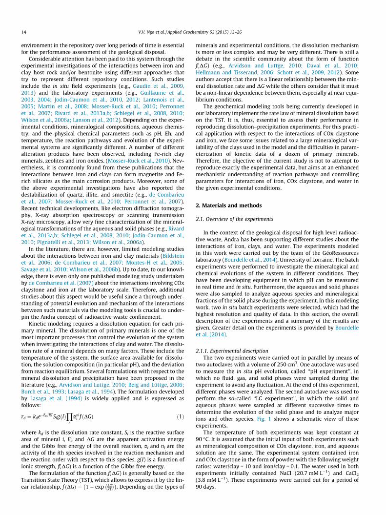
2.2.2. Initial conditions2.2.2.1. Composition of the experimental system. The mineral compo-sition used in the model is given in Table 1. The system containspowders of iron and COx clay, and water with respect to the ratiosof 10 and 0.1 for water/clay and iron/clay, respectively. There are
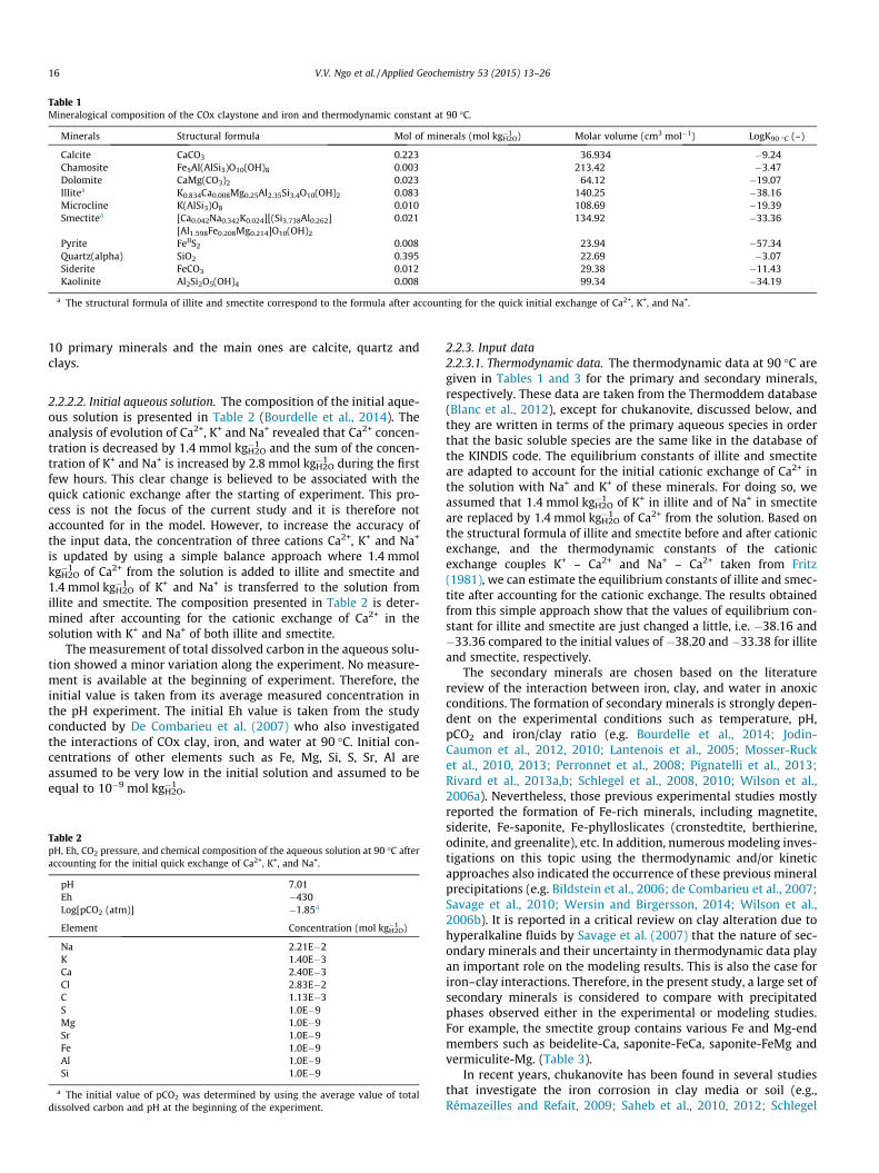
Table 1Mineralogical composition of the COx claystone and iron and thermodynamic constant at 90 �C.
Minerals Structural formula Mol of minerals (mol kg�1H2O) Molar volume (cm3 mol�1) LogK90 �C (–)
Calcite CaCO3 0.223 36.934 �9.24Chamosite Fe5Al(AlSi3)O10(OH)8 0.003 213.42 �3.47Dolomite CaMg(CO3)2 0.023 64.12 �19.07Illitea K0.834Ca0.008Mg0.25Al2.35Si3.4O10(OH)2 0.083 140.25 �38.16Microcline K(AlSi3)O8 0.010 108.69 �19.39Smectitea [Ca0.042Na0.342K0.024][(Si3.738Al0.262] 0.021 134.92 �33.36
[Al1.598Fe0.208Mg0.214]O10(OH)2
Pyrite FeIIS2 0.008 23.94 �57.34Quartz(alpha) SiO2 0.395 22.69 �3.07Siderite FeCO3 0.012 29.38 �11.43Kaolinite Al2Si2O5(OH)4 0.008 99.34 �34.19
a The structural formula of illite and smectite correspond to the formula after accounting for the quick initial exchange of Ca2+, K+, and Na+.
16 V.V. Ngo et al. / Applied Geochemistry 53 (2015) 13–26
10 primary minerals and the main ones are calcite, quartz andclays.
2.2.2.2. Initial aqueous solution. The composition of the initial aque-ous solution is presented in Table 2 (Bourdelle et al., 2014). Theanalysis of evolution of Ca2+, K+ and Na+ revealed that Ca2+ concen-tration is decreased by 1.4 mmol kg�1
H2O and the sum of the concen-tration of K+ and Na+ is increased by 2.8 mmol kg�1
H2O during the firstfew hours. This clear change is believed to be associated with thequick cationic exchange after the starting of experiment. This pro-cess is not the focus of the current study and it is therefore notaccounted for in the model. However, to increase the accuracy ofthe input data, the concentration of three cations Ca2+, K+ and Na+
is updated by using a simple balance approach where 1.4 mmolkg�1
H2O of Ca2+ from the solution is added to illite and smectite and1.4 mmol kg�1
H2O of K+ and Na+ is transferred to the solution fromillite and smectite. The composition presented in Table 2 is deter-mined after accounting for the cationic exchange of Ca2+ in thesolution with K+ and Na+ of both illite and smectite.
The measurement of total dissolved carbon in the aqueous solu-tion showed a minor variation along the experiment. No measure-ment is available at the beginning of experiment. Therefore, theinitial value is taken from its average measured concentration inthe pH experiment. The initial Eh value is taken from the studyconducted by De Combarieu et al. (2007) who also investigatedthe interactions of COx clay, iron, and water at 90 �C. Initial con-centrations of other elements such as Fe, Mg, Si, S, Sr, Al areassumed to be very low in the initial solution and assumed to beequal to 10�9 mol kg�1
H2O.
Table 2pH, Eh, CO2 pressure, and chemical composition of the aqueous solution at 90 �C afteraccounting for the initial quick exchange of Ca2+, K+, and Na+.
pH 7.01Eh �430Log[pCO2 (atm)] �1.85a
Element Concentration (mol kg�1H2O)
Na 2.21E�2K 1.40E�3Ca 2.40E�3Cl 2.83E�2C 1.13E�3S 1.0E�9Mg 1.0E�9Sr 1.0E�9Fe 1.0E�9Al 1.0E�9Si 1.0E�9
a The initial value of pCO2 was determined by using the average value of totaldissolved carbon and pH at the beginning of the experiment.
2.2.3. Input data2.2.3.1. Thermodynamic data. The thermodynamic data at 90 �C aregiven in Tables 1 and 3 for the primary and secondary minerals,respectively. These data are taken from the Thermoddem database(Blanc et al., 2012), except for chukanovite, discussed below, andthey are written in terms of the primary aqueous species in orderthat the basic soluble species are the same like in the database ofthe KINDIS code. The equilibrium constants of illite and smectiteare adapted to account for the initial cationic exchange of Ca2+ inthe solution with Na+ and K+ of these minerals. For doing so, weassumed that 1.4 mmol kg�1
H2O of K+ in illite and of Na+ in smectiteare replaced by 1.4 mmol kg�1
H2O of Ca2+ from the solution. Based onthe structural formula of illite and smectite before and after cationicexchange, and the thermodynamic constants of the cationicexchange couples K+ – Ca2+ and Na+ – Ca2+ taken from Fritz(1981), we can estimate the equilibrium constants of illite and smec-tite after accounting for the cationic exchange. The results obtainedfrom this simple approach show that the values of equilibrium con-stant for illite and smectite are just changed a little, i.e. �38.16 and�33.36 compared to the initial values of �38.20 and �33.38 for illiteand smectite, respectively.
The secondary minerals are chosen based on the literaturereview of the interaction between iron, clay, and water in anoxicconditions. The formation of secondary minerals is strongly depen-dent on the experimental conditions such as temperature, pH,pCO2 and iron/clay ratio (e.g. Bourdelle et al., 2014; Jodin-Caumon et al., 2012, 2010; Lantenois et al., 2005; Mosser-Rucket al., 2010, 2013; Perronnet et al., 2008; Pignatelli et al., 2013;Rivard et al., 2013a,b; Schlegel et al., 2008, 2010; Wilson et al.,2006a). Nevertheless, those previous experimental studies mostlyreported the formation of Fe-rich minerals, including magnetite,siderite, Fe-saponite, Fe-phylloslicates (cronstedtite, berthierine,odinite, and greenalite), etc. In addition, numerous modeling inves-tigations on this topic using the thermodynamic and/or kineticapproaches also indicated the occurrence of these previous mineralprecipitations (e.g. Bildstein et al., 2006; de Combarieu et al., 2007;Savage et al., 2010; Wersin and Birgersson, 2014; Wilson et al.,2006b). It is reported in a critical review on clay alteration due tohyperalkaline fluids by Savage et al. (2007) that the nature of sec-ondary minerals and their uncertainty in thermodynamic data playan important role on the modeling results. This is also the case foriron–clay interactions. Therefore, in the present study, a large set ofsecondary minerals is considered to compare with precipitatedphases observed either in the experimental or modeling studies.For example, the smectite group contains various Fe and Mg-endmembers such as beidelite-Ca, saponite-FeCa, saponite-FeMg andvermiculite-Mg. (Table 3).
In recent years, chukanovite has been found in several studiesthat investigate the iron corrosion in clay media or soil (e.g.,Rémazeilles and Refait, 2009; Saheb et al., 2010, 2012; Schlegel
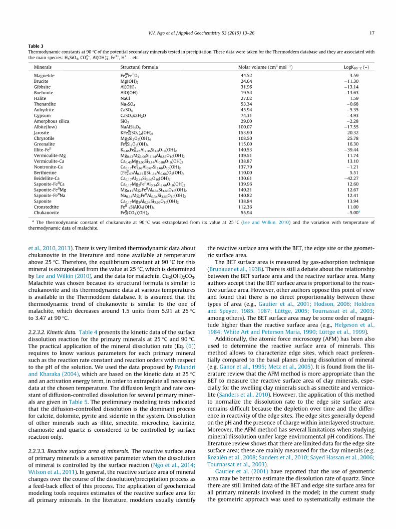
Table 3Thermodynamic constants at 90 �C of the potential secondary minerals tested in precipitation. These data were taken for the Thermoddem database and they are associated withthe main species: H4SiO4, CO3
2�, Al(OH)4�, Fe2+, H+. . . etc.
Minerals Structural formula Molar volume (cm3 mol�1) LogK90 �C (–)
Magnetite FeIII2 FeIIO4 44.52 3.59
Brucite Mg(OH)2 24.64 �11.30Gibbsite Al(OH)3 31.96 �13.14Boehmite AlO(OH) 19.54 �13.63Halite NaCl 27.02 1.59Thenardite Na2SO4 53.34 �0.68Anhydrite CaSO4 45.94 �5.35Gypsum CaSO4x2H2O 74.31 �4.93Amorphous silica SiO2 29.00 �2.28Albite(low) NaAlSi3O8 100.07 �17.55Jarosite KFeII
3(SO4)2(OH)6 153.90 20.32Chrysotile Mg3Si2O5(OH)4 108.50 25.78Greenalite FeII
3Si2O5(OH)4 115.00 16.30Illite-FeII K0.85FeII
0.25Al2.35Si3.4O10(OH)2 140.53 �39.44Vermiculite-Mg Mg0.43Mg3.00Si3.14Al0.86O10(OH)2 139.51 11.74Vermiculite-Ca Ca0.43Mg3.00Si3.14Al0.86O10(OH)2 138.87 13.10Nontronite-Ca Ca0.17FeII
1.67Al0.67Si3.66O10(OH)2 137.79 �1.21Berthierine (FeII
2.67Al0.33)(Si1.34Al0.66)O5(OH)4 110.00 5.51Beidellite-Ca Ca0.17Al2.34Si3.66O10(OH)2 130.61 �42.27Saponite-FeIICa Ca0.17Mg2FeIIAl0.34Si3.66O10(OH)2 139.96 12.60Saponite-FeIIMg Mg0.17Mg2FeIIAl0.34Si3.66O10(OH)2 140.21 12.67Saponite-FeIINa Na0.34Mg2FeIIAl0.34Si3.66O10(OH)2 140.82 12.41Saponite Ca0.17Mg3Al0.34Si3.66O10(OH)2 138.84 13.94Cronstedtite FeII
3SiAlO5(OH)4 112.36 11.00Chukanovite FeII
2(CO3)(OH)2 55.94 �5.00a
a The thermodynamic constant of chukanovite at 90 �C was extrapolated from its value at 25 �C (Lee and Wilkin, 2010) and the variation with temperature ofthermodynamic data of malachite.
V.V. Ngo et al. / Applied Geochemistry 53 (2015) 13–26 17
et al., 2010, 2013). There is very limited thermodynamic data aboutchukanovite in the literature and none available at temperatureabove 25 �C. Therefore, the equilibrium constant at 90 �C for thismineral is extrapolated from the value at 25 �C, which is determinedby Lee and Wilkin (2010), and the data for malachite, Cu2(OH)2CO3.Malachite was chosen because its structural formula is similar tochukanovite and its thermodynamic data at various temperaturesis available in the Thermoddem database. It is assumed that thethermodynamic trend of chukanovite is similar to the one ofmalachite, which decreases around 1.5 units from 5.91 at 25 �Cto 3.47 at 90 �C.
2.2.3.2. Kinetic data. Table 4 presents the kinetic data of the surfacedissolution reaction for the primary minerals at 25 �C and 90 �C.The practical application of the mineral dissolution rate (Eq. (6))requires to know various parameters for each primary mineralsuch as the reaction rate constant and reaction orders with respectto the pH of the solution. We used the data proposed by Palandriand Kharaka (2004), which are based on the kinetic data at 25 �Cand an activation energy term, in order to extrapolate all necessarydata at the chosen temperature. The diffusion length and rate con-stant of diffusion-controlled dissolution for several primary miner-als are given in Table 5. The preliminary modeling tests indicatedthat the diffusion-controlled dissolution is the dominant processfor calcite, dolomite, pyrite and siderite in the system. Dissolutionof other minerals such as illite, smectite, microcline, kaolinite,chamosite and quartz is considered to be controlled by surfacereaction only.
2.2.3.3. Reactive surface area of minerals. The reactive surface areaof primary minerals is a sensitive parameter when the dissolutionof mineral is controlled by the surface reaction (Ngo et al., 2014;Wilson et al., 2011). In general, the reactive surface area of mineralchanges over the course of the dissolution/precipitation process asa feed-back effect of this process. The application of geochemicalmodeling tools requires estimates of the reactive surface area forall primary minerals. In the literature, modelers usually identify
the reactive surface area with the BET, the edge site or the geomet-ric surface area.
The BET surface area is measured by gas-adsorption technique(Brunauer et al., 1938). There is still a debate about the relationshipbetween the BET surface area and the reactive surface area. Manyauthors accept that the BET surface area is proportional to the reac-tive surface area. However, other authors oppose this point of viewand found that there is no direct proportionality between thesetypes of area (e.g., Gautier et al., 2001; Hodson, 2006; Holdrenand Speyer, 1985, 1987; Lüttge, 2005; Tournassat et al., 2003;among others). The BET surface area may be some order of magni-tude higher than the reactive surface area (e.g., Helgeson et al.,1984; White Art and Peterson Maria, 1990; Lüttge et al., 1999).
Additionally, the atomic force microscopy (AFM) has been alsoused to determine the reactive surface area of minerals. Thismethod allows to characterize edge sites, which react preferen-tially compared to the basal planes during dissolution of mineral(e.g. Ganor et al., 1995; Metz et al., 2005). It is found from the lit-erature review that the AFM method is more appropriate than theBET to measure the reactive surface area of clay minerals, espe-cially for the swelling clay minerals such as smectite and vermicu-lite (Sanders et al., 2010). However, the application of this methodto normalize the dissolution rate to the edge site surface arearemains difficult because the depletion over time and the differ-ence in reactivity of the edge sites. The edge sites generally dependon the pH and the presence of charge within interlayered structure.Moreover, the AFM method has several limitations when studyingmineral dissolution under large environmental pH conditions. Theliterature review shows that there are limited data for the edge sitesurface area; these are mainly measured for the clay minerals (e.g.Rozalén et al., 2008; Sanders et al., 2010; Sayed Hassan et al., 2006;Tournassat et al., 2003).
Gautier et al. (2001) have reported that the use of geometricarea may be better to estimate the dissolution rate of quartz. Sincethere are still limited data of the BET and edge site surface area forall primary minerals involved in the model; in the current studythe geometric approach was used to systematically estimate the
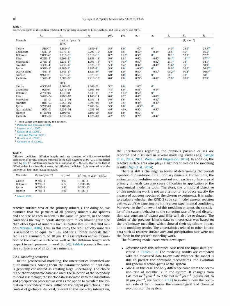
Table 4Kinetic constants of dissolution reaction of the primary minerals of COx claystone, and iron at 25 �C and 90 �C.
ka kn kb pHa pHb na nb Ea En Eb
Minerals (mol m�2 year�1) (kJ mol�1)25 �C
Calcite 1.58E+7b 4.88E+1b 4.88E+1a 5.5b 8.0a 1.00b 0a 14.5b 23.5b 23.5a,b
Chamosite 1.58E�2c 9.97E�6c 6.29E�10c 6.0c 9.5c 0.53c �0.44c 66.5f 45a 66.5b
Dolomite 2.03E+4b 9.31E�1b 9.31E�1a 8.7b 11.0a 0.50b 0a 36.1b 52.2b 52.2a
Illite 6.29E�5d 6.29E�8d 3.15E�13d 5.0d 8.8d 0.60d �0.60d 46a,d,e 14a,d,e 67a,d,e
Microcline 2.75E�3b 1.23E�5b 1.99E�14b 4.7b 10.7b 0.50b �0.82b 51.7b 38b 94.1b
Smectite 3.30E�4b 5.23E�6b 9.52E�10b 5.3b 9.4b 0.34b �0.40b 23.6b 35b 58.9b
Pyrite 9.52E�1b 8.88E+2b 8.88E+2a 5.9b 8.0a �0.50b 0a 56.9b 56.9b 56.9a,b
Quartz(alpha) 1.44E�4a 1.44E�6b 1.62E�9b 4.0a 5.9b 0.50a �0.50b 99.2a,b 90.1b 108.4b
Siderite 9.97E+1e 9.97E�2e 9.97E�2e 6.0a 8.0a 0.50 0a 61g 48g 48g
Kaolinite 1.54E�4b 2.08E�6b 2.81E�10b 6.0a 8.0a 0.78b �0.47b 65.9b 22.2b 17.9b
90 �CCalcite 4.50E+07 2.66E+02 2.66E+02 5.2a 8.0a 1.00b 0a
Chamosite 1.92E+0 2.57E�04 7.66E�08 7.3a 8.0 0.53c �0.44c
Dolomite 2.75E+05 4.04E+01 4.04E+01 7.7a 11.0a 0.50b 0a
Illite 5.49E�04 1.29E�07 1.16E�11 6.0a 6.7d 0.60d �0.60d
Microcline 1.15E�01 1.91E�04 1.78E�11 5.6a 8.6a 0.50b �0.82b
Smectite 1.81E�03 6.55E�05 6.69E�08 4.2a 7.5a 0.34b �0.40b
Pyrite 5.79E+01 5.40E+04 5.40E+04 5.9a 8.0a �0.50b 0a
Quartz(alpha) 1.95E�01 9.63E�04 4.05E�06 4.6a 4.8+a 0.50a �0.50b
Siderite 8.16E+03 3.19E+00 3.19E+00 6.8a 8.0a 0.50 0a
Kaolinite 1.80E�02 1.03E�05 1.02E�09 4.2a 8.5a 0.78b �0.47b
a These values are assessed by the authors.b Palandri and Kharaka (2004).c Lowson et al. (2005).d Köhler et al. (2003).e Tang and Martin (2011).f Brandt et al. (2003).g Golubev et al. (2009).
Table 5Diffusion coefficient, diffusion length, and rate constant of diffusion-controlleddissolution of several primary minerals of the COx claystone at 90 �C. ei is estimatedfrom Eq. (4). KD
i is determined from the assumption kDi ¼ DiCeq=ei . Due to the lack of
diffusion data for minerals in water, the diffusion coefficient, Di, is assumed to be thesame for all four investigated minerals.
Minerals Dia (m2 year�1) ei (lm) kD
i (mol m year�1 kg�1H2O)
Calcite 9.75E�3 4.93 1.14E�6Dolomite 9.75E�3 6.72 1.23E�16Pyrite 9.75E�3 5.40 8.25E�55Siderite 9.75E�3 5.90 6.19E�9
a Madé (1991).
18 V.V. Ngo et al. / Applied Geochemistry 53 (2015) 13–26
reactive surface area of the primary minerals. For doing so, weassumed that the particles of all primary minerals are spheresand the size of each mineral is the same. In general, in the sameconditions the clay minerals always form much smaller grain sizethan other types of minerals such as carbonates, sulfates and oxi-des (Meunier, 2006). Thus, in this study the radius of clay mineralsis assumed to be equal to 1 lm, and for all other minerals theirradius are assumed to be 10 lm. This assumption allows estima-tion of the reactive surface as well as the diffusion length withrespect to each primary mineral (Eq. (4)). Table 6 presents the reac-tive surface area of all primary minerals.
2.2.4. Modeling scenariosIn the geochemical modeling, the uncertainties identified are
quite numerous. Among them, the parameterization of input datais generally considered as creating large uncertainty. The choiceof the thermodynamic database used, the selection of the secondarymineral assemblage, the kinetic data associated with the dissolutionand precipitation processes as well as the option to calculate the for-mation of secondary mineral influence the output predictions. In thecontext of geological disposal, relevant to the iron–clay interaction,
the uncertainties regarding the previous possible causes arereported and discussed in several modeling studies (e.g. Savageet al., 2007, 2011; Wersin and Birgersson, 2014). In addition, thereactive surface area also plays a significant role on the modelingresults (Ngo et al., 2014).
There is still a challenge in terms of determining the overallequation of dissolution for all primary minerals. Furthermore, theestimates of dissolution rate constant and reactive surface area ofprimary minerals can also cause difficulties in application of thegeochemical modeling tools. Therefore, the primordial objectiveof this modeling work is not an attempt to reproduce exactly themeasured aqueous species of the chosen experiments. It is ratherto evaluate whether the KINDIS code can model general reactionpathways of the experiments in the given experimental conditions.Moreover, in the framework of this modeling attempt, the sensitiv-ity of the system behavior to the corrosion rate of Fe and dissolu-tion rate constant of quartz and illite will also be evaluated. Thechoice of the previous kinetic data to investigate was based onthe preliminary modeling, which showed their significant impacton the modeling results. The uncertainties related to other kineticdata such as reactive surface area and precipitation rate were notthe focus in the present modeling work.
The following model cases were developed:
� Reference case: this reference case used the input data pre-sented in Tables 1–6. The modeling results are comparedwith the measured data to evaluate whether the model isable to predict the dominant mechanisms, the evolutionand general reaction-paths of the system.
� Case 1: in this case, the only difference came from the corro-sion rate of metallic Fe in the system. It changes from1.41 mol m�2 year�1 to 2.82 mol m�2 year�1 (equivalent to20 lm year�1, see Section 2.1.2) to evaluate how the corro-sion rate of Fe influences the mineralogical and chemicalevolutions of the system.
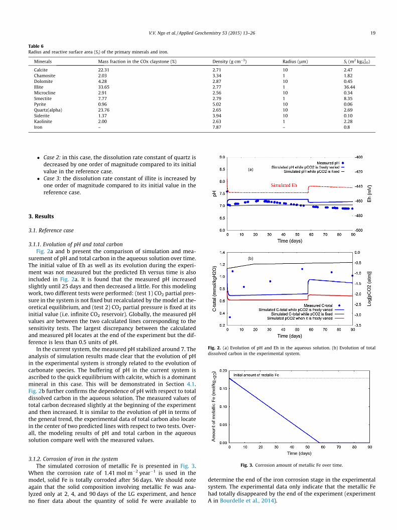
Table 6Radius and reactive surface area (Si) of the primary minerals and iron.
Minerals Mass fraction in the COx claystone (%) Density (g cm�3) Radius (lm) Si (m2 kg�1H2O)
Calcite 22.31 2.71 10 2.47Chamosite 2.03 3.34 1 1.82Dolomite 4.28 2.87 10 0.45Illite 33.65 2.77 1 36.44Microcline 2.91 2.56 10 0.34Smectite 7.77 2.79 1 8.35Pyrite 0.96 5.02 10 0.06Quartz(alpha) 23.76 2.65 10 2.69Siderite 1.37 3.94 10 0.10Kaolinite 2.00 2.63 1 2.28Iron – 7.87 – 0.8
Fig. 2. (a) Evolution of pH and Eh in the aqueous solution. (b) Evolution of totaldissolved carbon in the experimental system.
V.V. Ngo et al. / Applied Geochemistry 53 (2015) 13–26 19
� Case 2: in this case, the dissolution rate constant of quartz isdecreased by one order of magnitude compared to its initialvalue in the reference case.
� Case 3: the dissolution rate constant of illite is increased byone order of magnitude compared to its initial value in thereference case.
3. Results
3.1. Reference case
3.1.1. Evolution of pH and total carbonFig. 2a and b present the comparison of simulation and mea-
surement of pH and total carbon in the aqueous solution over time.The initial value of Eh as well as its evolution during the experi-ment was not measured but the predicted Eh versus time is alsoincluded in Fig. 2a. It is found that the measured pH increasedslightly until 25 days and then decreased a little. For this modelingwork, two different tests were performed: (test 1) CO2 partial pres-sure in the system is not fixed but recalculated by the model at the-oretical equilibrium, and (test 2) CO2 partial pressure is fixed at itsinitial value (i.e. infinite CO2 reservoir). Globally, the measured pHvalues are between the two calculated lines corresponding to thesensitivity tests. The largest discrepancy between the calculatedand measured pH locates at the end of the experiment but the dif-ference is less than 0.5 units of pH.
In the current system, the measured pH stabilized around 7. Theanalysis of simulation results made clear that the evolution of pHin the experimental system is strongly related to the evolution ofcarbonate species. The buffering of pH in the current system isascribed to the quick equilibrium with calcite, which is a dominantmineral in this case. This will be demonstrated in Section 4.1.Fig. 2b further confirms the dependence of pH with respect to totaldissolved carbon in the aqueous solution. The measured values oftotal carbon decreased slightly at the beginning of the experimentand then increased. It is similar to the evolution of pH in terms ofthe general trend, the experimental data of total carbon also locatein the center of two predicted lines with respect to two tests. Over-all, the modeling results of pH and total carbon in the aqueoussolution compare well with the measured values.
Fig. 3. Corrosion amount of metallic Fe over time.
3.1.2. Corrosion of iron in the systemThe simulated corrosion of metallic Fe is presented in Fig. 3.When the corrosion rate of 1.41 mol m�2 year�1 is used in themodel, solid Fe is totally corroded after 56 days. We should noteagain that the solid composition involving metallic Fe was ana-lyzed only at 2, 4, and 90 days of the LG experiment, and henceno finer data about the quantity of solid Fe were available to
determine the end of the iron corrosion stage in the experimentalsystem. The experimental data only indicate that the metallic Fehad totally disappeared by the end of the experiment (experimentA in Bourdelle et al., 2014).
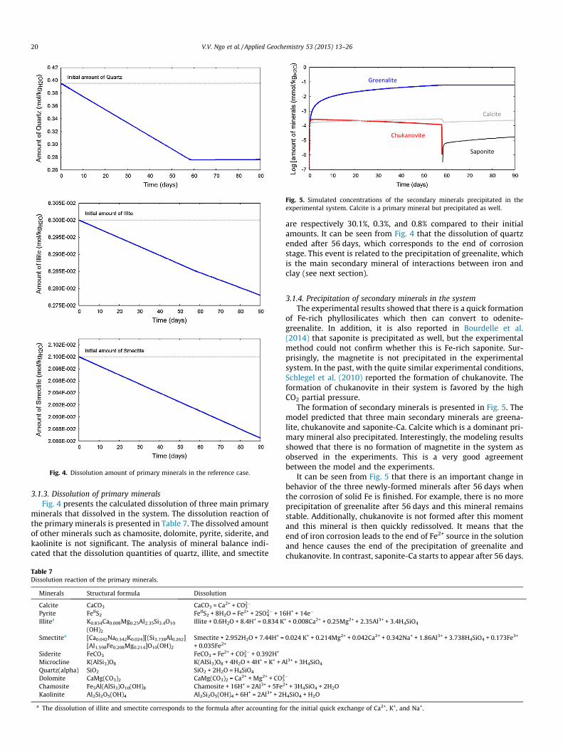
Fig. 4. Dissolution amount of primary minerals in the reference case.
Chukanovite
Saponite
Calcite
Greenalite
Fig. 5. Simulated concentrations of the secondary minerals precipitated in theexperimental system. Calcite is a primary mineral but precipitated as well.
20 V.V. Ngo et al. / Applied Geochemistry 53 (2015) 13–26
3.1.3. Dissolution of primary mineralsFig. 4 presents the calculated dissolution of three main primary
minerals that dissolved in the system. The dissolution reaction ofthe primary minerals is presented in Table 7. The dissolved amountof other minerals such as chamosite, dolomite, pyrite, siderite, andkaolinite is not significant. The analysis of mineral balance indi-cated that the dissolution quantities of quartz, illite, and smectite
Table 7Dissolution reaction of the primary minerals.
Minerals Structural formula Dissolution
Calcite CaCO3 CaCO3 = Ca2+ + CO32�
Pyrite FeIIS2 FeIIS2 + 8H2O = Fe2+ + 2SO42� + 16
Illitea K0.834Ca0.008Mg0.25Al2.35Si3.4O10
(OH)2
Illite + 0.6H2O + 8.4H+ = 0.834 K
Smectitea [Ca0.042Na0.342K0.024][(Si3.738Al0.262] Smectite + 2.952H2O + 7.44H+ =+ 0.035Fe2+[Al1.598Fe0.208Mg0.214]O10(OH)2
Siderite FeCO3 FeCO3 = Fe2+ + CO32� + 0.392H+
Microcline K(AlSi3)O8 K(AlSi3)O8 + 4H2O + 4H+ = K+ + AQuartz(alpha) SiO2 SiO2 + 2H2O = H4SiO4
Dolomite CaMg(CO3)2 CaMg(CO3)2 = Ca2+ + Mg2+ + CO32
Chamosite Fe5Al(AlSi3)O10(OH)8 Chamosite + 16H+ = 2Al3+ + 5Fe2
Kaolinite Al2Si2O5(OH)4 Al2Si2O5(OH)4 + 6H+ = 2Al3+ + 2H
a The dissolution of illite and smectite corresponds to the formula after accounting fo
are respectively 30.1%, 0.3%, and 0.8% compared to their initialamounts. It can be seen from Fig. 4 that the dissolution of quartzended after 56 days, which corresponds to the end of corrosionstage. This event is related to the precipitation of greenalite, whichis the main secondary mineral of interactions between iron andclay (see next section).
3.1.4. Precipitation of secondary minerals in the systemThe experimental results showed that there is a quick formation
of Fe-rich phyllosilicates which then can convert to odenite-greenalite. In addition, it is also reported in Bourdelle et al.(2014) that saponite is precipitated as well, but the experimentalmethod could not confirm whether this is Fe-rich saponite. Sur-prisingly, the magnetite is not precipitated in the experimentalsystem. In the past, with the quite similar experimental conditions,Schlegel et al. (2010) reported the formation of chukanovite. Theformation of chukanovite in their system is favored by the highCO2 partial pressure.
The formation of secondary minerals is presented in Fig. 5. Themodel predicted that three main secondary minerals are greena-lite, chukanovite and saponite-Ca. Calcite which is a dominant pri-mary mineral also precipitated. Interestingly, the modeling resultsshowed that there is no formation of magnetite in the system asobserved in the experiments. This is a very good agreementbetween the model and the experiments.
It can be seen from Fig. 5 that there is an important change inbehavior of the three newly-formed minerals after 56 days whenthe corrosion of solid Fe is finished. For example, there is no moreprecipitation of greenalite after 56 days and this mineral remainsstable. Additionally, chukanovite is not formed after this momentand this mineral is then quickly redissolved. It means that theend of iron corrosion leads to the end of Fe2+ source in the solutionand hence causes the end of the precipitation of greenalite andchukanovite. In contrast, saponite-Ca starts to appear after 56 days.
H+ + 14e�+ + 0.008Ca2+ + 0.25Mg2+ + 2.35Al3+ + 3.4H4SiO4
0.024 K+ + 0.214Mg2+ + 0.042Ca2+ + 0.342Na+ + 1.86Al3+ + 3.738H4SiO4 + 0.173Fe3+
l3+ + 3H4SiO4
�
+ + 3H4SiO4 + 2H2O4SiO4 + H2O
r the initial quick exchange of Ca2+, K+, and Na+.
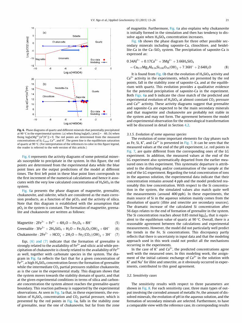
Fig. 6. Phase diagrams of quartz and different minerals that potentially precipitatedat 90 �C in the experimental system: (a) when fixing log[pO2 (atm)] = �60, (b) whenfixing log[a(Mg2+)/a2(H+)] = 9. The red points are determined from the measuredconcentrations of Si, Ctotal, Ca2+, and H+. The green line is the equilibrium saturationof quartz at 90 �C. (For interpretation of the references to color in this figure legend,the reader is referred to the web version of this article.)
V.V. Ngo et al. / Applied Geochemistry 53 (2015) 13–26 21
Fig. 6 represents the activity diagrams of some potential miner-als susceptible to precipitate in the system. In this figure, the redpoints are determined from the experimental data while the bluepoint lines are the output predictions of the model at differenttimes. The first left point in these blue point lines corresponds tothe first increment of the numerical calculations and hence it asso-ciates with the very low calculated concentrations of H4SiO4 in thesystem.
Fig. 6a presents the phase diagram of magnetite, greenalite,chukanovite, and siderite, which are considered as the main corro-sion products, as a function of the pCO2 and the activity of silica.Note that this diagram is established with the assumption thatpO2 in the system is constant. The formation of magnetite, greena-lite and chukanovite are written as follows:
Magnetite : 2Fe3þ þ Fe2þ þ 4H2O ¼ Fe3O4 þ 8Hþ ð5ÞGreenalite : 3Fe2þ þ 2H4SiO4 þH2O ¼ Fe3Si2O5ðOHÞ4 þ 6Hþ ð6ÞChukanovite : 2Fe2þ þHCO�3 þ 2H2O ¼ Fe2ðCO3ÞðOHÞ2 þ 3Hþ ð7Þ
Eqs. (6) and (7) indicate that the formation of greenalite isstrongly related to the availability of Fe2+ and silicic acid while pre-cipitation of chukanovite is closely related to the availability of Fe2+
as well, together with carbonate species in the system. The dia-gram in Fig. 6a reflects the fact that for a given concentration ofFe2+, a high H4SiO4 concentration favors the formation of greenalitewhile the intermediate CO2 partial pressures stabilize chukanovite,as is the case in the experimental study. This diagram shows thatthe system moves towards the stability domain of quartz, and thatat the given experimental conditions in terms of silica and carbon-ate concentration the system almost reaches the greenalite-quartzboundary. This reaction pathway is supported by the experimentalobservations. As seen in Fig. 5a that, in these experiments, the evo-lution of H4SiO4 concentration and CO2 partial pressure, which ispresented by the red points in Fig. 6a, falls in the stability zoneof greenalite, near the one of chukanovite, but far from the zone
of magnetite. Furthermore, Fig. 6a also explains why chukanoviteis initially formed in the simulation and then has tendency to dis-solve again when H4SiO4 concentration increases.
Fig. 6b shows the phase diagram for three other possible sec-ondary minerals including saponite-Ca, clinochlore, and beidel-lite-Ca in the Ca–SiO2 system. The precipitation of saponite-Ca isexpressed as:
0:34Al3þ þ 0:17Ca2þ þ 3Mg2þ þ 3:66H4SiO4
¼ Ca0:17Mg3Al0:34Si3:66O10ðOHÞ2 þ 7:36Hþ þ 2:64H2O ð8Þ
It is found from Fig. 6b that the evolution of H4SiO4 activity andCa2+ activity in the experiments, which are presented by the redpoints, fall in the stability zone of saponite-Ca, and at the equilib-rium with quartz. This evolution provides a qualitative evidencefor the potential precipitation of saponite-Ca in the experiment.Both Figs. 6a and b indicate the close match of the predicted andexperimental evolution of H4SiO4 at almost constant CO2 pressureand Ca2+ activity. These activity diagrams suggest that greenaliteand saponite-Ca are expected to be the main secondary mineralsand that magnetite and chukanovite are probably not stable inthe system and may not form. The agreement between the modeland experimental observation for the mineralogical transformationwill be discussed in detail in Section 4.2.
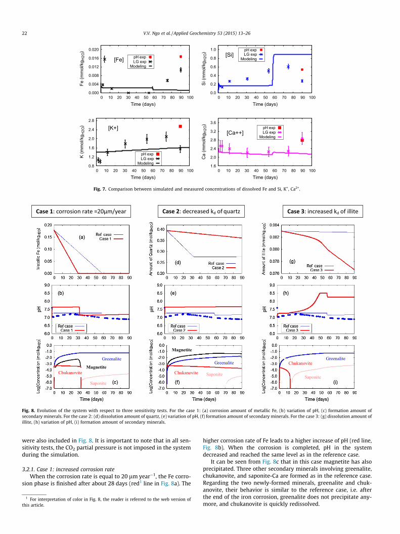
3.1.5. Evolution of some aqueous speciesThe evolution of some important elements for clay phases such
as Fe, Si, K+, and Ca2+ is presented in Fig. 7. It can be seen that themeasured values at the end of the pH experiment, i.e. red points inFig. 7, are quite different from the corresponding ones of the LGexperiment. In addition, the measured values at the end of theLG experiment also systematically departed from the earlier mea-sured ones in this experiment. This systematic departure is attrib-uted to the disturbing and/or contamination of the sample at theend of the LG experiment. Regarding the total concentration of ionsin the aqueous solution, the experimental data indicate that theirconcentration remains around 4 ppb and the model predicted rea-sonably this low concentration. With respect to the Si concentra-tion in the system, the simulated values also match quite wellthe measurements (around 400 ppb). In these experiments, themain source of Si in the aqueous solution mainly comes from thedissolution of quartz (illite and smectite are secondary sources).The dramatic increase of the calculated Si concentration after56 days relates to the end of formation of greenalite in the system.The Si concentration reaches about 0.85 mmol kg�1
H2O that is equiv-alent to the equilibrium value of quartz at 90 �C. Overall, there is areasonable agreement between the calculations and experimentalmeasurements. However, the model did not particularly well predictthe trends in the Fe, Si concentrations. This discrepancy partlyreflects that there is uncertainty in input data and that the modelingapproach used in this work could not predict all the mechanismsoccurring in the experiments.
In the case of K+ and Ca2+, the predicted concentrations agreewell with the measured ones. In this modeling work, the assign-ment of the initial cationic exchange of Ca2+ in the solution withK+ and Na+ for illite and smectite, as it obviously occurred in exper-iments, contributed to this good agreement.
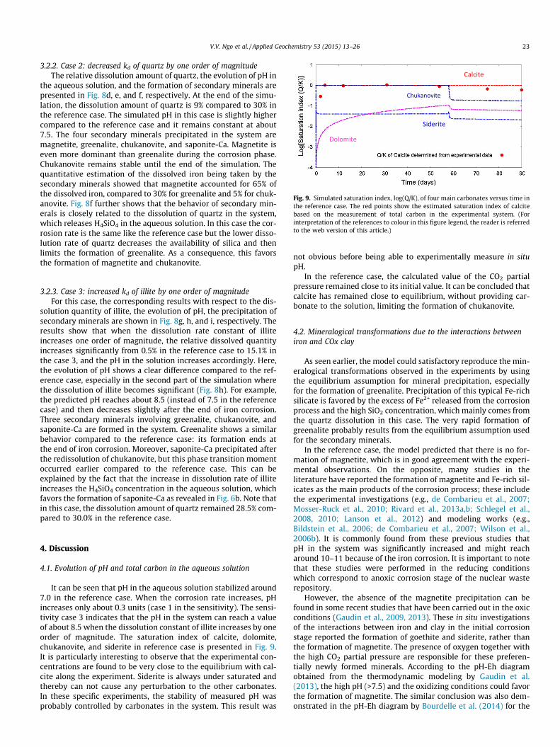
3.2. Sensitivity cases
The sensitivity results with respect to three parameters areshown in Fig. 8. For each sensitivity case, three main types of out-put involving the corroded amount of metallic Fe, the amount of dis-solved minerals, the evolution of pH in the aqueous solution, and theformation of secondary minerals are selected. Furthermore, to havea comparable view with the reference case, its corresponding results
0.000
0.004
0.008
0.012
0.016
0.020
0 10 20 30 40 50 60 70 80 90 100
Fe (m
mol
/kg H
2O)
Time (days)
[Fe] pH expLG exp
Modeling
0.0
0.2
0.4
0.6
0.8
1.0
0 10 20 30 40 50 60 70 80 90 100
Si (
mm
ol/k
g H2O
)
Time (days)
[Si]pH expLG exp
Modeling
0.8
1.2
1.6
2.0
2.4
2.8
0 10 20 30 40 50 60 70 80 90 100
K (m
mol
/kg H
2O)
Time (days)
[K+]
pH expLG exp
Modeling 1.6
2.0
2.4
2.8
3.2
3.6
0 10 20 30 40 50 60 70 80 90 100
Ca
(mm
ol/k
g H2O
)
Time (days)
[Ca++]pH expLG exp
Modeling
Fig. 7. Comparison between simulated and measured concentrations of dissolved Fe and Si, K+, Ca2+.
Case 2: decreased kd of Case 3: increased kd of illiteCase 1: corrosion rate =20µm/year
Greenalite
Saponite
ChukanoviteMagnetite
Magnetite
Greenalite
Chukanovite Saponite
Greenalite
Saponite
Chukanovite
quartz
Fig. 8. Evolution of the system with respect to three sensitivity tests. For the case 1: (a) corrosion amount of metallic Fe, (b) variation of pH, (c) formation amount ofsecondary minerals. For the case 2: (d) dissolution amount of quartz, (e) variation of pH, (f) formation amount of secondary minerals. For the case 3: (g) dissolution amount ofillite, (h) variation of pH, (i) formation amount of secondary minerals.
22 V.V. Ngo et al. / Applied Geochemistry 53 (2015) 13–26
were also included in Fig. 8. It is important to note that in all sen-sitivity tests, the CO2 partial pressure is not imposed in the systemduring the simulation.
3.2.1. Case 1: increased corrosion rateWhen the corrosion rate is equal to 20 lm year�1, the Fe corro-
sion phase is finished after about 28 days (red1 line in Fig. 8a). The
1 For interpretation of color in Fig. 8, the reader is referred to the web version ofthis article.
higher corrosion rate of Fe leads to a higher increase of pH (red line,Fig. 8b). When the corrosion is completed, pH in the systemdecreased and reached the same level as in the reference case.
It can be seen from Fig. 8c that in this case magnetite has alsoprecipitated. Three other secondary minerals involving greenalite,chukanovite, and saponite-Ca are formed as in the reference case.Regarding the two newly-formed minerals, greenalite and chuk-anovite, their behavior is similar to the reference case, i.e. afterthe end of the iron corrosion, greenalite does not precipitate any-more, and chukanovite is quickly redissolved.
Calcite
Dolomite
Siderite
Chukanovite
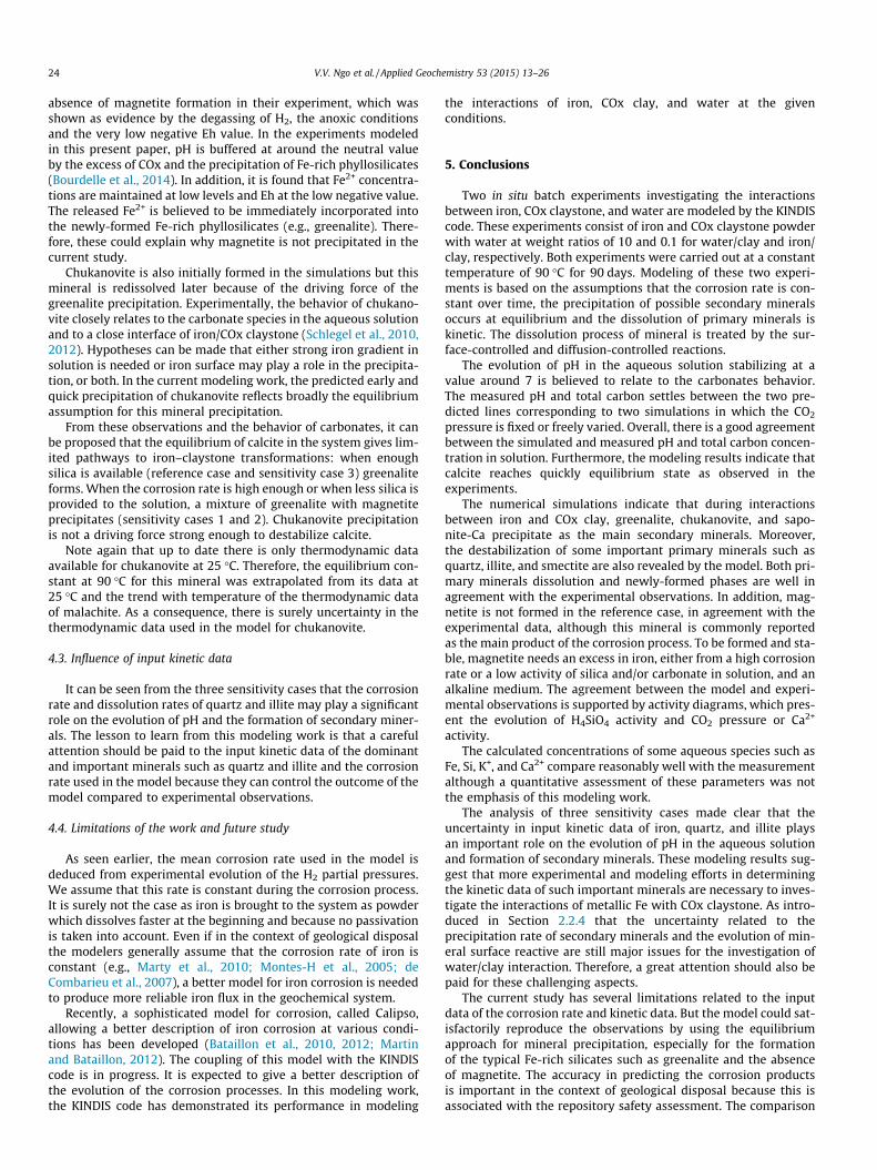
Fig. 9. Simulated saturation index, log(Q/K), of four main carbonates versus time inthe reference case. The red points show the estimated saturation index of calcitebased on the measurement of total carbon in the experimental system. (Forinterpretation of the references to colour in this figure legend, the reader is referredto the web version of this article.)
V.V. Ngo et al. / Applied Geochemistry 53 (2015) 13–26 23
3.2.2. Case 2: decreased kd of quartz by one order of magnitudeThe relative dissolution amount of quartz, the evolution of pH in
the aqueous solution, and the formation of secondary minerals arepresented in Fig. 8d, e, and f, respectively. At the end of the simu-lation, the dissolution amount of quartz is 9% compared to 30% inthe reference case. The simulated pH in this case is slightly highercompared to the reference case and it remains constant at about7.5. The four secondary minerals precipitated in the system aremagnetite, greenalite, chukanovite, and saponite-Ca. Magnetite iseven more dominant than greenalite during the corrosion phase.Chukanovite remains stable until the end of the simulation. Thequantitative estimation of the dissolved iron being taken by thesecondary minerals showed that magnetite accounted for 65% ofthe dissolved iron, compared to 30% for greenalite and 5% for chuk-anovite. Fig. 8f further shows that the behavior of secondary min-erals is closely related to the dissolution of quartz in the system,which releases H4SiO4 in the aqueous solution. In this case the cor-rosion rate is the same like the reference case but the lower disso-lution rate of quartz decreases the availability of silica and thenlimits the formation of greenalite. As a consequence, this favorsthe formation of magnetite and chukanovite.
3.2.3. Case 3: increased kd of illite by one order of magnitudeFor this case, the corresponding results with respect to the dis-
solution quantity of illite, the evolution of pH, the precipitation ofsecondary minerals are shown in Fig. 8g, h, and i, respectively. Theresults show that when the dissolution rate constant of illiteincreases one order of magnitude, the relative dissolved quantityincreases significantly from 0.5% in the reference case to 15.1% inthe case 3, and the pH in the solution increases accordingly. Here,the evolution of pH shows a clear difference compared to the ref-erence case, especially in the second part of the simulation wherethe dissolution of illite becomes significant (Fig. 8h). For example,the predicted pH reaches about 8.5 (instead of 7.5 in the referencecase) and then decreases slightly after the end of iron corrosion.Three secondary minerals involving greenalite, chukanovite, andsaponite-Ca are formed in the system. Greenalite shows a similarbehavior compared to the reference case: its formation ends atthe end of iron corrosion. Moreover, saponite-Ca precipitated afterthe redissolution of chukanovite, but this phase transition momentoccurred earlier compared to the reference case. This can beexplained by the fact that the increase in dissolution rate of illiteincreases the H4SiO4 concentration in the aqueous solution, whichfavors the formation of saponite-Ca as revealed in Fig. 6b. Note thatin this case, the dissolution amount of quartz remained 28.5% com-pared to 30.0% in the reference case.
4. Discussion
4.1. Evolution of pH and total carbon in the aqueous solution
It can be seen that pH in the aqueous solution stabilized around7.0 in the reference case. When the corrosion rate increases, pHincreases only about 0.3 units (case 1 in the sensitivity). The sensi-tivity case 3 indicates that the pH in the system can reach a valueof about 8.5 when the dissolution constant of illite increases by oneorder of magnitude. The saturation index of calcite, dolomite,chukanovite, and siderite in reference case is presented in Fig. 9.It is particularly interesting to observe that the experimental con-centrations are found to be very close to the equilibrium with cal-cite along the experiment. Siderite is always under saturated andthereby can not cause any perturbation to the other carbonates.In these specific experiments, the stability of measured pH wasprobably controlled by carbonates in the system. This result was
not obvious before being able to experimentally measure in situpH.
In the reference case, the calculated value of the CO2 partialpressure remained close to its initial value. It can be concluded thatcalcite has remained close to equilibrium, without providing car-bonate to the solution, limiting the formation of chukanovite.
4.2. Mineralogical transformations due to the interactions betweeniron and COx clay
As seen earlier, the model could satisfactory reproduce the min-eralogical transformations observed in the experiments by usingthe equilibrium assumption for mineral precipitation, especiallyfor the formation of greenalite. Precipitation of this typical Fe-richsilicate is favored by the excess of Fe2+ released from the corrosionprocess and the high SiO2 concentration, which mainly comes fromthe quartz dissolution in this case. The very rapid formation ofgreenalite probably results from the equilibrium assumption usedfor the secondary minerals.
In the reference case, the model predicted that there is no for-mation of magnetite, which is in good agreement with the experi-mental observations. On the opposite, many studies in theliterature have reported the formation of magnetite and Fe-rich sil-icates as the main products of the corrosion process; these includethe experimental investigations (e.g., de Combarieu et al., 2007;Mosser-Ruck et al., 2010; Rivard et al., 2013a,b; Schlegel et al.,2008, 2010; Lanson et al., 2012) and modeling works (e.g.,Bildstein et al., 2006; de Combarieu et al., 2007; Wilson et al.,2006b). It is commonly found from these previous studies thatpH in the system was significantly increased and might reacharound 10–11 because of the iron corrosion. It is important to notethat these studies were performed in the reducing conditionswhich correspond to anoxic corrosion stage of the nuclear wasterepository.
However, the absence of the magnetite precipitation can befound in some recent studies that have been carried out in the oxicconditions (Gaudin et al., 2009, 2013). These in situ investigationsof the interactions between iron and clay in the initial corrosionstage reported the formation of goethite and siderite, rather thanthe formation of magnetite. The presence of oxygen together withthe high CO2 partial pressure are responsible for these preferen-tially newly formed minerals. According to the pH-Eh diagramobtained from the thermodynamic modeling by Gaudin et al.(2013), the high pH (>7.5) and the oxidizing conditions could favorthe formation of magnetite. The similar conclusion was also dem-onstrated in the pH-Eh diagram by Bourdelle et al. (2014) for the
24 V.V. Ngo et al. / Applied Geochemistry 53 (2015) 13–26
absence of magnetite formation in their experiment, which wasshown as evidence by the degassing of H2, the anoxic conditionsand the very low negative Eh value. In the experiments modeledin this present paper, pH is buffered at around the neutral valueby the excess of COx and the precipitation of Fe-rich phyllosilicates(Bourdelle et al., 2014). In addition, it is found that Fe2+ concentra-tions are maintained at low levels and Eh at the low negative value.The released Fe2+ is believed to be immediately incorporated intothe newly-formed Fe-rich phyllosilicates (e.g., greenalite). There-fore, these could explain why magnetite is not precipitated in thecurrent study.
Chukanovite is also initially formed in the simulations but thismineral is redissolved later because of the driving force of thegreenalite precipitation. Experimentally, the behavior of chukano-vite closely relates to the carbonate species in the aqueous solutionand to a close interface of iron/COx claystone (Schlegel et al., 2010,2012). Hypotheses can be made that either strong iron gradient insolution is needed or iron surface may play a role in the precipita-tion, or both. In the current modeling work, the predicted early andquick precipitation of chukanovite reflects broadly the equilibriumassumption for this mineral precipitation.
From these observations and the behavior of carbonates, it canbe proposed that the equilibrium of calcite in the system gives lim-ited pathways to iron–claystone transformations: when enoughsilica is available (reference case and sensitivity case 3) greenaliteforms. When the corrosion rate is high enough or when less silica isprovided to the solution, a mixture of greenalite with magnetiteprecipitates (sensitivity cases 1 and 2). Chukanovite precipitationis not a driving force strong enough to destabilize calcite.
Note again that up to date there is only thermodynamic dataavailable for chukanovite at 25 �C. Therefore, the equilibrium con-stant at 90 �C for this mineral was extrapolated from its data at25 �C and the trend with temperature of the thermodynamic dataof malachite. As a consequence, there is surely uncertainty in thethermodynamic data used in the model for chukanovite.
4.3. Influence of input kinetic data
It can be seen from the three sensitivity cases that the corrosionrate and dissolution rates of quartz and illite may play a significantrole on the evolution of pH and the formation of secondary miner-als. The lesson to learn from this modeling work is that a carefulattention should be paid to the input kinetic data of the dominantand important minerals such as quartz and illite and the corrosionrate used in the model because they can control the outcome of themodel compared to experimental observations.
4.4. Limitations of the work and future study
As seen earlier, the mean corrosion rate used in the model isdeduced from experimental evolution of the H2 partial pressures.We assume that this rate is constant during the corrosion process.It is surely not the case as iron is brought to the system as powderwhich dissolves faster at the beginning and because no passivationis taken into account. Even if in the context of geological disposalthe modelers generally assume that the corrosion rate of iron isconstant (e.g., Marty et al., 2010; Montes-H et al., 2005; deCombarieu et al., 2007), a better model for iron corrosion is neededto produce more reliable iron flux in the geochemical system.
Recently, a sophisticated model for corrosion, called Calipso,allowing a better description of iron corrosion at various condi-tions has been developed (Bataillon et al., 2010, 2012; Martinand Bataillon, 2012). The coupling of this model with the KINDIScode is in progress. It is expected to give a better description ofthe evolution of the corrosion processes. In this modeling work,the KINDIS code has demonstrated its performance in modeling
the interactions of iron, COx clay, and water at the givenconditions.
5. Conclusions
Two in situ batch experiments investigating the interactionsbetween iron, COx claystone, and water are modeled by the KINDIScode. These experiments consist of iron and COx claystone powderwith water at weight ratios of 10 and 0.1 for water/clay and iron/clay, respectively. Both experiments were carried out at a constanttemperature of 90 �C for 90 days. Modeling of these two experi-ments is based on the assumptions that the corrosion rate is con-stant over time, the precipitation of possible secondary mineralsoccurs at equilibrium and the dissolution of primary minerals iskinetic. The dissolution process of mineral is treated by the sur-face-controlled and diffusion-controlled reactions.
The evolution of pH in the aqueous solution stabilizing at avalue around 7 is believed to relate to the carbonates behavior.The measured pH and total carbon settles between the two pre-dicted lines corresponding to two simulations in which the CO2
pressure is fixed or freely varied. Overall, there is a good agreementbetween the simulated and measured pH and total carbon concen-tration in solution. Furthermore, the modeling results indicate thatcalcite reaches quickly equilibrium state as observed in theexperiments.
The numerical simulations indicate that during interactionsbetween iron and COx clay, greenalite, chukanovite, and sapo-nite-Ca precipitate as the main secondary minerals. Moreover,the destabilization of some important primary minerals such asquartz, illite, and smectite are also revealed by the model. Both pri-mary minerals dissolution and newly-formed phases are well inagreement with the experimental observations. In addition, mag-netite is not formed in the reference case, in agreement with theexperimental data, although this mineral is commonly reportedas the main product of the corrosion process. To be formed and sta-ble, magnetite needs an excess in iron, either from a high corrosionrate or a low activity of silica and/or carbonate in solution, and analkaline medium. The agreement between the model and experi-mental observations is supported by activity diagrams, which pres-ent the evolution of H4SiO4 activity and CO2 pressure or Ca2+
activity.The calculated concentrations of some aqueous species such as
Fe, Si, K+, and Ca2+ compare reasonably well with the measurementalthough a quantitative assessment of these parameters was notthe emphasis of this modeling work.
The analysis of three sensitivity cases made clear that theuncertainty in input kinetic data of iron, quartz, and illite playsan important role on the evolution of pH in the aqueous solutionand formation of secondary minerals. These modeling results sug-gest that more experimental and modeling efforts in determiningthe kinetic data of such important minerals are necessary to inves-tigate the interactions of metallic Fe with COx claystone. As intro-duced in Section 2.2.4 that the uncertainty related to theprecipitation rate of secondary minerals and the evolution of min-eral surface reactive are still major issues for the investigation ofwater/clay interaction. Therefore, a great attention should also bepaid for these challenging aspects.
The current study has several limitations related to the inputdata of the corrosion rate and kinetic data. But the model could sat-isfactorily reproduce the observations by using the equilibriumapproach for mineral precipitation, especially for the formationof the typical Fe-rich silicates such as greenalite and the absenceof magnetite. The accuracy in predicting the corrosion productsis important in the context of geological disposal because this isassociated with the repository safety assessment. The comparison
V.V. Ngo et al. / Applied Geochemistry 53 (2015) 13–26 25
of these modeling results with the experimental data has proven tobe helpful in understanding the processes at the interface betweenclay and iron, the controlling mechanism and parameters of theprocesses. To further confirm the robustness of the modeling, abetter coupling between geochemistry, corrosion, and transportphenomena has to be tested and assessed. Our understanding ofclay–iron interactions could be improved by ongoing laboratoryexperiments and geochemical modeling of these experiments, withupscaling to repository scale systems.
Acknowledgements
We are grateful to the experimental team, Régine Mosser-Ruck,Michel Cathelineau, Frank Bourdelle, Laurent Truche, Isabella Pig-natelli, Catherine Lorgeoux, Chistophe Roszypal, in the GéoRes-sources laboratory, Université de Lorraine, for providing theexperimental data. We would also like to thank the Agence natio-nale pour la gestion des déchets radioactifs (Andra) for the finan-cial support of this work. We warmly thank Dr. James Wilsonand the anonymous reviewer and associate editor for their veryhelpful and constructive comments.
References
Arvidson, R.S., Luttge, A., 2010. Mineral dissolution kinetics as a function of distancefrom equilibrium – new experimental results. Chem. Geol. 269 (1–2), 79–88.
Bataillon, C., Bouchon, F., Chainais-Hillairet, C., Desgranges, C., Hoarau, E., Martin, F.,Perrin, S., Tupin, M., Talandier, J., 2010. Corrosion modelling of iron based alloyin nuclear waste repository. Electrochim. Acta 55 (15), 4451–4467.
Bataillon, C., Bouchon, F., Chainais-Hillairet, C., Fuhrmann, J., Hoarau, E., Touzani, R.,2012. Numerical methods for the simulation of a corrosion model with movingoxide layer. J. Comput. Phys. 231 (18), 6213–6231.
Beig, M.S., Lüttge, A., 2006. Albite dissolution kinetics as a function of distance fromequilibrium: implications for natural feldspar weathering. Geochim.Cosmochim. Acta 70 (6), 1402–1420.
Bildstein, O., Trotignon, L., Perronnet, M., Jullien, M., 2006. Modelling iron–clayinteractions in deep geological disposal conditions. Phys. Chem. Earth 31 (10–14), 618–625.
Blanc, P., Lassin, A., Piantone, P., Azaroual, M., Jacquemet, N., Fabbri, A., Gaucher,E.C., 2012. Thermoddem: a geochemical database focused on low temperaturewater/rock interactions and waste materials. Appl. Geochem. 27 (10), 2107–2116.
Bourdelle, F., Truche, L., Pignatelli, I., Mosser-Ruck, R., Lorgeoux, C., Roszypal, C.,Michau, N., 2014. Iron–clay interactions under hydrothermal conditions:impact of specific surface area of metallic iron on reaction pathway. Chem.Geol. 381, 194–205.
Brandt, F., Bosbach, D., Krawczyk-Barsch, E., Arnold, T., Bernhard, G., 2003. Chloritedissolution in the acid ph-range: a combined microscopic and macroscopicapproach. Geochim. Cosmochim. Acta 67 (8), 1451–1461.
Brunauer, S., Emmett, P.H., Teller, E., 1938. Adsorption of gases in multimolecularlayers. J. Am. Chem. Soc. 60 (2), 309–319.
Burch, T.E., Nagy, K.L., Lasaga, A.C., 1993. Free energy dependence of albitedissolution kinetics at 80 �C and pH 8.8. Chem. Geol. 105 (1–3), 137–162.
Daval, D., Hellmann, R., Corvisier, J., Tisserand, D., Martinez, I., Guyot, F., 2010.Dissolution kinetics of diopside as a function of solution saturation state:macroscopic measurements and implications for modeling of geological storageof CO2. Geochim. Cosmochim. Acta 74 (9), 2615–2633.
de Combarieu, G., Barboux, P., Minet, Y., 2007. Iron corrosion in Callovo-Oxfordianargilite: from experiments to thermodynamic/kinetic modelling. Phys. Chem.Earth 32 (1–7), 346–358.
Fritz, B., 1981. Etude thermodynamique et modélisation des réactionshydrothermales et diagénétiques. Thèse d’état de l’Université Louis Pasteur,Institut de Géologie.
Ganor, J., Mogollón, J.L., Lasaga, A.C., 1995. The effect of pH on kaolinite dissolutionrates and on activation energy. Geochim. Cosmochim. Acta 59 (6), 1037–1052.
Gaudin, A., Gaboreau, S., Tinseau, E., Bartier, D., Petit, S., Grauby, O., Foct, F., Beaufort,D., 2009. Mineralogical reactions in the Tournemire argillite after in-situinteraction with steels. Appl. Clay Sci. 43 (2), 196–207. http://dx.doi.org/10.1016/j.clay.2008.08.007.
Gaudin, A., Bartier, D., Truche, L., Tinseau, E., Foct, F., Dyja, V., Maillet, A., Beaufort,D., 2013. First corrosion stages in Tournemire claystone/steel interaction: in situexperiment and modelling approach. Appl. Clay Sci. 83–84, 457–468.
Gautier, J.M., Oelkers, E.H., Schott, J., 2001. Are quartz dissolution rates proportionalto B.E.T. surface areas? Geochim. Cosmochim. Acta 65 (7), 1059–1070.
Golubev, S.V., Bénézeth, P., Schott, J., Dandurand, J.L., Castillo, A., 2009. Sideritedissolution kinetics in acidic aqueous solutions from 25 to 100 �C and 0 to50 atm pCO2. Chem. Geol. 265 (1–2), 13–19.
Guillaume, D., Neaman, A., Cathelineau, M., Mosser-Ruck, R., Peiffert, C.,Abdelmoula, M., Dubessy, J., Villieras, F., Baronnet, A., Michau, N., 2003.Experimental synthesis of chlorite from smectite at 300 �C in the presence ofmetallic Fe. Clay Miner. 38 (3), 281–302.
Guillaume, D., Neaman, A., Cathelineau, M., Mosser-Ruck, R., Peiffert, C.,Abdelmoula, M., Dubessy, J., Villiéras, F., Michau, N., 2004. Experimental studyof the transformation of smectite at 80 and 300 �C in the presence of Fe oxides.Clay Miner. 39 (1), 17–34.
Helgeson, H.C., Murphy, W.M., Aagaard, P., 1984. Thermodynamic and kineticconstraints on reaction rates among minerals and aqueous solutions. II. Rateconstants, effective surface area, and the hydrolysis of feldspar. Geochim.Cosmochim. Acta 48 (12), 2405–2432.
Hellmann, R., Tisserand, D., 2006. Dissolution kinetics as a function of the Gibbs freeenergy of reaction: an experimental study based on albite feldspar. Geochim.Cosmochim. Acta 70 (2), 364–383.
Hodson, M.E., 2006. Does reactive surface area depend on grain size? Results frompH 3, 25 �C far-from-equilibrium flow-through dissolution experiments onanorthite and biotite. Geochim. Cosmochim. Acta 70 (7), 1655–1667.
Holdren Jr, G.R., Speyer, P.M., 1985. Reaction rate-surface area relationships duringthe early stages of weathering-I. Initial observations. Geochimica etCosmochimica Acta 49 (3), 675–681.
Holdren Jr, G.R., Speyer, P.M., 1987. Reaction rate-surface area relationships duringthe early stages of weathering. II. Data on eight additional feldspars. Geochim.Cosmochim. Acta 51 (9), 2311–2318.
Jeschke, A.A., Dreybrodt, W., 2002. Dissolution rates of minerals and their relation tosurface morphology. Geochim. Cosmochim. Acta 66 (17), 3055–3062.
Jodin-Caumon, M.C., Mosser-Ruck, R., Rousset, D., Randi, A., Cathelineau, M.,Michau, N., 2010. Effect of a thermal gradient on iron–clay interactions. ClaysClay Miner. 58 (5), 667–681.
Jodin-Caumon, M.C., Mosser-Ruck, R., Randi, A., Pierron, O., Cathelineau, M., Michau,N., 2012. Mineralogical evolution of a claystone after reaction with iron underthermal gradient. Clays Clay Miner. 60 (5), 443–455.
Köhler, S.J., Dufaud, F., Oelkers, E.H., 2003. An experimental study of illitedissolution kinetics as a function of ph from 1.4 to 12.4 and temperaturefrom 5 to 50 �C. Geochim. Cosmochim. Acta 67 (19), 3583–3594. http://dx.doi.org/10.1016/s0016-7037(03)00163-7.
Lanson, B., Lantenois, S., Van Aken, P.A., Bauer, A., Plançon, A., 2012. Experimentalinvestigation of smectite interaction with metal iron at 80 �c: structuralcharacterization of newly formed Fe-rich phyllosilicates. Am. Mineral. 97 (5–6), 864–871.
Lantenois, S., Lanson, B., Muller, F., Bauer, A., Jullien, M., Plançon, A., 2005.Experimental study of smectite interaction with metal Fe at low temperature: 1.Smectite destabilization. Clays Clay Miner. 53 (6), 597–612.
Lasaga, A.C., 1986. Metamorphic reaction rate laws and development of isograds.Mineral. Mag. 50 (3), 359–373.
Lasaga, A.C., Soler, J.M., Ganor, J., Burch, T.E., Nagy, K.L., 1994. Chemical weatheringrate laws and global geochemical cycles. Geochim. Cosmochim. Acta 58 (10),2361–2386.
Lee, T.R., Wilkin, R.T., 2010. Iron hydroxy carbonate formation in zerovalent ironpermeable reactive barriers: characterization and evaluation of phase stability.J. Contam. Hydrol. 116 (1–4), 47–57.
Lowson, R.T., Comarmond, M.C.J., Rajaratnam, G., Brown, P.L., 2005. The kinetics ofthe dissolution of chlorite as a function of pH and at 25 �C. Geochim.Cosmochim. Acta 69 (7), 1687–1699. http://dx.doi.org/10.1016/j.gca.2004.09.028.
Lüttge, A., 2005. Etch pit coalescence, surface area, and overall mineral dissolutionrates. Am. Mineral. 90 (11–12), 1776–1783.
Lüttge, A., Bolton, E.W., Lasaga, A.C., 1999. An interferometric study of thedissolution kinetics of anorthite: the role of reactive surface area. Am. J. Sci.299 (7–9), 652–678.
Madé, B., 1991. Modélisation thermodynamique et cinétique des réactionsgéochimiques dans les intéractions eau-roche. Université Louis Pasteur.
Madé, B., Clément, A., Fritz, B., 1994. Modeling mineral/solution interactions: thethermodynamic and kinetic code KINDISP. Comput. Geosci. 20 (9), 1347–1363.
Martin, F.A., Bataillon, C., 2012. Modelling of the evolution of iron passivity: solvingthe moving boundaries problem. In: Materials Research Society SymposiumProceedings, April 9–13, San Francisco, CA, United States, pp. 275 –280.10.1557/opl.2012.586.
Martin, F.A., Bataillon, C., Schlegel, M.L., 2008. Corrosion of iron and low alloyedsteel within a water saturated brick of clay under anaerobic deep geologicaldisposal conditions: an integrated experiment. J. Nucl. Mater. 379 (1–3), 80–90.
Marty, N.C.M., Fritz, B., Clément, A., Michau, N., 2010. Modelling the long termalteration of the engineered bentonite barrier in an underground radioactivewaste repository. Appl. Clay Sci. 47 (1–2), 82–90.
Metz, V., Raanan, H., Pieper, H., Bosbach, D., Ganor, J., 2005. Towards theestablishment of a reliable proxy for the reactive surface area of smectite.Geochim. Cosmochim. Acta 69 (10), 2581–2591. http://dx.doi.org/10.1016/j.gca.2004.11.009.
Meunier, A., 2006. Why are clay minerals small? Clay Miner. 41 (2), 551–566.Montes-H, G., Marty, N., Fritz, B., Clement, A., Michau, N., 2005. Modelling of long-
term diffusion-reaction in a bentonite barrier for radioactive wasteconfinement. Appl. Clay Sci. 30 (3–4), 181–198.
Morse, J.W., Arvidson, R.S., 2002. The dissolution kinetics of major sedimentarycarbonate minerals. Earth Sci. Rev. 58 (1–2), 51–84.
Mosser-Ruck, R., Cathelineau, M., Guillaume, D., Charpentier, D., Rousset, D., Barres,O., Michau, N., 2010. Effects of temperature, pH, and iron/clay and liquid/clay
26 V.V. Ngo et al. / Applied Geochemistry 53 (2015) 13–26
ratios on experimental conversion of dioctahedral smectite to berthierine,chlorite, vermiculite, or saponite. Clays Clay Miner. 58 (2), 280–291.
Mosser-Ruck, R., Pignatelli, I., Bourdelle, F., Truche, L., Bartier, D., Cathelineau, M.,2013. Etude du système Verre-Fer-Argilite: Rôles du pH, du redox et de la pCO2
sur la nature des phases minérales ferrifères néoformées au contact des colis etstabilité de ces phases lors d’un refroidissement entre 90 �C et 30 �C. vol.ANDRA report, RP 0G2R.13.0001, pp. 147.
Murphy, W.M., Oelkers, E.H., Lichtner, P.C., 1989. Surface reaction versus diffusioncontrol of mineral dissolution and growth rates in geochemical processes.Chem. Geol. 78 (3–4), 357–380.
Ngo, V.V., Delalande, M., Clément, A., Michau, N., Fritz, B., 2014. Coupled transport-reaction modeling of the long-term interaction between iron, bentonite andCallovo-Oxfordian claystone in radioactive waste confinement systems. Appl.Clay Sci. 101, 430–443.
Palandri, J.L., Kharaka, Y.K., 2004. A compilation of rate parameters of water–mineral interaction kinetics for application to geochemical modeling. In: U.S.Department of the Interior U.S. Geological Survey 1849 C. Street, NWWashington, DC 20240.
Perronnet, M., Villiéras, F., Jullien, M., Razafitianamaharavo, A., Raynal, J., Bonnin, D.,2007. Towards a link between the energetic heterogeneities of the edge faces ofsmectites and their stability in the context of metallic corrosion. Geochim.Cosmochim. Acta 71 (6), 1463–1479.
Perronnet, M., Jullien, M., Villiéras, F., Raynal, J., Bonnin, D., Bruno, G., 2008.Evidence of a critical content in Fe(0) on FoCa7 bentonite reactivity at 80 �C.Appl. Clay Sci. 38 (3–4), 187–202.
Pignatelli, I., Mugnaioli, E., Hybler, J., Mosser-Ruck, R., Cathelineau, M., Michau, N.,2013. A multi-technique characterization of cronstedtite synthesized by iron–clay interaction in a step-by-step cooling procedure. Clays Clay Miner. 61 (4),277–289.
Rémazeilles, C., Refait, P., 2009. Fe(II) hydroxycarbonate Fe2(OH)2CO3 (chukanovite)as iron corrosion product: synthesis and study by Fourier Transform InfraredSpectroscopy. Polyhedron 28 (4), 749–756.
Rivard, C., Montargès-Pelletier, E., Vantelon, D., Pelletier, M., Karunakaran, C.,Michot, L.J., Villieras, F., Michau, N., 2013a. Combination of multi-scale andmulti-edge X-ray spectroscopy for investigating the products obtained from theinteraction between kaolinite and metallic iron in anoxic conditions at 90 �C.Phys. Chem. Miner. 40 (2), 115–132.
Rivard, C., Pelletier, M., Michau, N., Razafitianamaharavo, A., Bihannic, I.,Abdelmoula, M., Ghanbaja, J., Villiéras, F., 2013b. Berthierine-like mineralformation and stability during the interaction of kaolinite with metallic iron at90 �c under anoxic and oxic conditions. Am. Mineral. 98 (1), 163–180.
Rozalén, M.L., Huertas, F.J., Brady, P.V., Cama, J., García-Palma, S., Linares, J., 2008.Experimental study of the effect of pH on the kinetics of montmorillonitedissolution at 25 �C. Geochim. Cosmochim. Acta 72 (17), 4224–4253.
Saheb, M., Descostes, M., Neff, D., Matthiesen, H., Michelin, A., Dillmann, P., 2010.Iron corrosion in an anoxic soil: comparison between thermodynamicmodelling and ferrous archaeological artefacts characterised along with thelocal in situ geochemical conditions. Appl. Geochem. 25 (12), 1937–1948.
Saheb, M., Berger, P., Raimbault, L., Neff, D., Dillmann, P., 2012. Investigation of ironlong-term corrosion mechanisms in anoxic media using deuterium tracing. J.Nucl. Mater. 423 (1–3), 61–66.
Sanders, R.L., Washton, N.M., Mueller, K.T., 2010. Measurement of the reactivesurface area of clay minerals using solid-state NMR studies of a probe molecule.J. Phys. Chem. C 114 (12), 5491–5498.
Savage, D., Walker, C., Arthur, R., Rochelle, C., Oda, C., Takase, H., 2007. Alteration ofbentonite by hyperalkaline fluids: a review of the role of secondary minerals.Phys. Chem. Earth 32 (1–7), 287–297.
Savage, D., Watson, C., Benbow, S., Wilson, J., 2010. Modelling iron–bentoniteinteractions. Appl. Clay Sci. 47 (1–2), 91–98.
Savage, D., Arthur, R., Watson, C., Wilson, J., Strömberg, B., 2011. Testinggeochemical models of bentonite pore water evolution against laboratoryexperimental data. Phys. Chem. Earth 36 (17–18), 1817–1829.
Sayed Hassan, M., Villieras, F., Gaboriaud, F., Razafitianamaharavo, A., 2006. AFMand low-pressure argon adsorption analysis of geometrical properties ofphyllosilicates. J. Colloid Interface Sci. 296 (2), 614–623.
Schlegel, M.L., Bataillon, C., Benhamida, K., Blanc, C., Menut, D., Lacour, J.L., 2008.Metal corrosion and argillite transformation at the water-saturated, high-temperature iron–clay interface. A microscopic-scale study. Appl. Geochem. 23(9), 2619–2633.
Schlegel, M.L., Bataillon, C., Blanc, C., Prêt, D., Eddy, F., 2010. Anodic activation of ironcorrosion in clay media under water-saturated conditions at 90 �C:characterization of the corrosion interface. Environ. Sci. Technol. 44 (4), 1503–1508.
Schlegel, M.L., Bataillon, C., Blanc, C., Foy, E., Brucker, F., 2013. From the ex-situsteel-clay to the in situ steel-porewater interfaces: comparing the results ofArCorr and MCO experiments. In: 4ième Réunion plénière du Groupement deLaboratoires Verre/Fer/Argile, GL-VFA Andra. 17–18 Juine, 2013, Paris, France(personal communication).
Schott, J., Pokrovsky, O.S., Oelkers, E.H., 2009. The link between mineral dissolution/precipitation kinetics and solution chemistry. Rev. Mineral. Geochem. 70, 207–258.
Schott, J., Oelkers, E.H., Bénézeth, P., Goddéris, Y., François, L., 2012. Can accuratekinetic laws be created to describe chemical weathering? Comptes Rendus –Geoscience 344 (11–12), 568–585.
Tang, Y., Martin, S.T., 2011. Siderite dissolution in the presence of chromate.Geochim. Cosmochim. Acta 75 (17), 4951–4962. http://dx.doi.org/10.1016/j.gca.2011.06.024.
Tournassat, C., Neaman, A., Villéras, F., Bosbach, D., Charlet, L., 2003.Nanomorphology of montmorillonite particles: estimation of the clay edgesorption site density by low-pressure gas adsorption and AFM observations.Am. Mineral. 88 (11–12 Part 2), 1989–1995.
Wersin, P., Birgersson, M., 2014. Reactive transport modelling of iron–bentoniteinteraction within the KBS-3H disposal concept: the Olkiluoto site as a casestudy. Geol. Soc. Lond. Spec. Publ. 400. http://dx.doi.org/10.1144/sp400.24.
White Art, F., Peterson Maria, L., 1990. Role of reactive-surface-area characterizationin geochemical kinetic models. Chemical Modeling of Aqueous Systems II, ACSSymposium Series, vol. 416. American Chemical Society, pp. 461–475.
Wilson, J., Cressey, G., Cressey, B., Cuadros, J., Ragnarsdottir, K.V., Savage, D., Shibata,M., 2006a. The effect of iron on montmorillonite stability. (II) Experimentalinvestigation. Geochim. Cosmochim. Acta 70 (2), 323–336.
Wilson, J., Savage, D., Cuadros, J., Shibata, M., Ragnarsdottir, K.V., 2006b. The effectof iron on montmorillonite stability. (I) Background and thermodynamicconsiderations. Geochim. Cosmochim. Acta 70 (2), 306–322.
Wilson, J., Savage, D., Bond, A., Watson, S., Pusch, R., Bennett, D., 2011. Bentonite: areview of key properties, processes and issues for consideration in the UKcontext. In: vol. Quintessa Report for NDA RWMD, Report number: QRS-1378ZG-1. Oxfordshire, United Kingdom.
Zhang, J.W., Nancollas, G.H., 1990. Mechanisms of growth and dissolution ofsparingly soluble salts. Rev. Mineral. Geochem. 23 (1), 365–396.


![“What is ν · [G D’Ambrosio et al., NPB 645 (2002) 155, hep-ph/0207036] Gauge invariant kinetic terms vs. Yukawa interactions Q¯](https://img.pdfslide.net/doc/110x75/5f5e375f660c196c2f50c27a/aoewhat-is-g-daambrosio-et-al-npb-645-2002-155-hep-ph0207036-gauge.jpg)


![Neutrino Oscillation Workshop · [G D’Ambrosio et al., NPB 645 (2002) 155, hep-ph/0207036] Gauge invariant kinetic terms vs. Yukawa interactions Q¯](https://img.pdfslide.net/doc/110x75/5f5e375f660c196c2f50c27b/neutrino-oscillation-workshop-g-daambrosio-et-al-npb-645-2002-155-hep-ph0207036.jpg)