Embed Size (px)
Citation preview

Kocher, Martin G.; Lucks, Konstantin E. und Schindler,
David:
Unleashing Animal Spirits - Self-Control and
Overpricing in Experimental Asset Markets
Munich Discussion Paper No. 2016-3
Department of Economics
University of Munich
Volkswirtschaftliche Fakultät
Ludwig-Maximilians-Universität München
Online at https://doi.org/10.5282/ubm/epub.27572

Unleashing Animal Spirits - Self-Control and Overpricing in
Experimental Asset Markets∗
Martin G. Kocher† Konstantin E. Lucks‡ David Schindler§
February 29, 2016
Abstract
One possible determinant of overpricing on asset markets is a lack of self-control abilities
of traders. Self-control is the individual capacity to override or inhibit undesired behavioral
tendencies such as impulses and to refrain from acting on them. We implement the first
experiment that is able to address a potential causal relationship between self-control abilities
and systematic overpricing on financial markets by introducing an exogenous variation of self-
control abilities. Our experimental conditions seek to detect some of the channels through which
individual self-control problems could transmit into irrational exuberance on the aggregate
level. We observe a strong effect of inhibited self-control abilities on market overpricing. Our
findings are furthermore robust to reducing self-control abilities only for a moderate share of
traders in a market. Low self-control traders engage in more speculative behavior early on,
but because others imitate their trading patterns, they do not end up earning less and are not
driven out of the market.
JEL codes: G02, G11, G12, D53, D84
Keywords: Behavioral finance, trader behavior, self control, experimental asset markets,
overpricing
∗We thank participants at numerous conferences and seminars. The paper benefited from many helpful commentsby Pablo Branas-Garza, Ernst Fehr, Michael Kirchler, Charles Noussair, Simeon Schudy and Stefan Trautmann.
†Corresponding Author, [email protected], +49 (0) 89 2180 9726, University of Munich, Department ofEconomics, Geschwister-Scholl-Platz 1, D-80539 Munich, Germany; Queensland University of Technology, Brisbane,Australia; and University of Gothenburg, Sweden.
‡[email protected], +49 (0) 89 2180 9776, University of Munich, Department of Economics,Geschwister-Scholl-Platz 1, D-80539 Munich, Germany.
§[email protected], +49 (0) 89 2180 9728, University of Munich, Department of Economics,Geschwister-Scholl-Platz 1, D-80539 Munich, Germany.
1
1 Introduction
“Even apart from the instability due to speculation, there is the instability due to the
characteristic of human nature that a large proportion of our positive activities depend
on spontaneous optimism rather than mathematical expectations, whether moral or
hedonistic or economic. Most, probably, of our decisions to do something positive (...)
can only be taken as the result of animal spirits – a spontaneous urge to action rather
than inaction, and not as the outcome of a weighted average of quantitative benefits
multiplied by quantitative probabilities.”1
John Maynard Keynes
Keynes famously saw “animal spirits” at the root of many (financial) decisions, potentially causing
price exaggerations on the aggregate market level. As often in Keynes’ work, the term “animal spir-
its” is not well-delineated. It alludes to optimism, instincts, urges, emotions, and similar concepts.
In this paper we assess the notion that a lack of self-control abilities may lead to price exaggerations
on asset markets, and we analyze how the lack of self-control abilities is associated to emotions and
trading behavior. In psychology, self-control abilities and willpower are defined as the capacities
to override or inhibit undesired behavioral tendencies such as impulses and to refrain from acting
on them (Tangney et al., 2004). Self-control is necessary to guard oneself against undue optimism,
actions motivated by emotional responses, and impulsive decisions. Furthermore, self-control is
required in order to stick to plans made in the past.
That self-control is considered relevant for investor success is also evident from statements of well-
known investors and from popular guidebooks on the psychology of investing. For instance, Warren
Buffet emphasizes that “success in investing doesn’t correlate with I.Q. once you’re above the level
of 25. Once you have ordinary intelligence, what you need is the temperament to control the
urges that get other people into trouble in investing.”2 Similarly, anecdotal evidence from rogue
traders on markets show that they completely lost their self-control abilities. In a study by Lo
et al. (2005) involving day traders from an online training program participants stated attributes
related to self-control as the most important determinants of trading success.3 In a similar spirit,
Fenton-O’Creevy et al. (2011) report distinct differences in emotion regulation strategies among
traders of different experience and performance levels from qualitative interviews with professional
traders. Therefore, correlational and casual evidence suggests that self-control matters for trading
success on an individual level.
1Source: Keynes (1936), p. 136.2http://www.businessweek.com/1999/99_27/b3636006.htm3They quote attributes such as persistence, tenacity, perseverance, patience, discipline, planning, controlling
emotions, and (lack of) impulsivity as crucial (Lo et al., 2005, table 3).
2

The major challenge to overcome is to exogenously vary self-control abilities in order to obtain
causal inference on the impact of self-control abilities on behavior and market outcomes. A first
step is to use the experimental laboratory and affect state self-control levels of traders. Most of the
available techniques draw on the concept of self-control depletion or exhaustion. Our experimental
identification rests on the assumption that self-control is a limited resource and that it is variable
over time on the individual level. Evidence for these two characteristics is abundant (e.g. Baumeister
et al., 1998; Gailliot et al., 2012). While validated survey measures for trait self-control exist, they
can only provide correlational inference.
This paper is the first to provide empirical evidence on the causal effects of a variation in self-
control abilities on trading outcomes.4 In the spirit of Keynes we concentrate on aggregate market
outcomes in a first experiment and extend our analysis to individual behavior and performance
in a second experiment. We use a well-understood financial market setup in the experimental
laboratory (Smith et al., 1988; Kirchler et al., 2012; Noussair and Tucker, 2013; Palan, 2013; Eckel
and Fullbrunn, 2015) to investigate whether an exogenous variation in self-control abilities of traders
leads to overpricing and irrational exuberance. This experimental asset market is known for its basic
tendency to exhibit overpricing; it features a dividend-bearing asset with decreasing fundamental
value.
In order to deplete self-control abilities before the start of the market, we employ the Stroop
task (Stroop, 1935), which is one of the most commonly used tasks in psychology experiments for
modulating self-control (Hagger et al., 2010). It is easy to administer, it can be implemented in
an exhausting/depleting version and in an easy version, and it allows for additional controls. The
majority of studies that use both survey measures and behavioral measures of self-control conclude
that the effects of state self-control interventions are qualitatively similar to those of trait self-
control levels (e.g. Schmeichel and Zell, 2007). Hence, even if our experiment is confined to the
laboratory setting and to a variation in state self-control, it is likely that it extends to real-world
situations in which also trait self-control matters.
Our main finding is a significantly higher level of overpricing on markets where traders’ self-control
abilities have been depleted, compared to markets with traders whose self-control abilities have not
been depleted. If markets are populated by both depleted and non-depleted traders the effect is
similar in size and also highly significant. Obviously, having some self-control depleted traders on
a market suffices to create the additional over-pricing effect.
Behavior on markets is path-dependent, choices are endogenous to other choices, and traders imitate
each other. Nonetheless, we are able to provide robust evidence from control variables, from trading
4However, there is a quickly growing empirical literature on the effects of self-control abilities on decision makingin other domains relevant to economists (see, for instance, Beshears et al. (2015).
3

and from survey questions that can explain the additional overpricing with depleted self-control
abilities. First, there is no direct effect of self-control depletion on risk attitudes or cognitive
abilities of traders, which could explain our findings. Second, self-control depleted traders do not
trade significantly less than non-depleted traders. Third, several indicators show that self-control
depleted traders follow stronger speculative motives earlier on when trading. In other words, they
contribute more to the creation of overpricing, and non-depleted traders jump on this bandwaggon.
Fourth, stronger emotional arousal in the market is related to being self-control depleted. In short,
traders become more impulsive and potentially rely less on cognitive skills, when they cannot resort
to their full self-control resources.
The remaining paper is organized as follows: Section 2 gives an overview of the literature related
to our research question, and in section 3, we explain and motivate our experimental design. Con-
sequently, section 4 presents the results from our main experiment, and section 5 reports on an
additional experiment that allows us both to test the robustness of our initial results and to better
understand how self-control depletion translates into overpricing and how traders’ behavior and
decision processes might be affected by the treatment. We discuss potential channels explaining
our findings in section 6. Section 7 concludes the paper.
2 Related Literature
Our literature overview focuses on the two aspects in the economics and psychology literature that
are most relevant for our study: self-control and experimental asset markets. As already said,
self-control abilities and willpower are defined as the capacities to override or inhibit undesired
behavioral tendencies such as impulses and to refrain from acting on them. There are different
theoretical approaches in psychology and in economics that take self-control abilities and potential
self-control problems into account.
First, self-control can straightforwardly be related to dual-systems perspectives of decision making.
As outlined by Kahneman (2011), these perspectives share the general assumption that structurally
different systems of information processing underlie the production of impulsive, largely automatic
forms of behavior, on the one hand (system 1), and deliberate, largely controlled forms of behavior,
on the other hand (system 2). System 2 is effortful and requires self-control resources.5 Thus,
if resources are low, reflective operations may be impaired, leading to a dominance of impulsive
reactions that could be in conflict with objective reasoning. From this perspective, reducing self-
5Note that the division of system 1 as automatic and system 2 as controlled describes a tendency; there are bothautomatic and conscious processes involved in exerting self-control and giving in to temptation, respectively (cf.Kotabe and Hofmann, 2015).
4

control abilities can be interpreted as increasing the role of the (impulsive) system 1 in decision
making (Hofmann et al., 2009).
Second, and very much related to dual-system perspectives, economists have used dual-self models
of impulse control (see, for instance, Thaler and Shefrin (1981) and Fudenberg and Levine (2006)) in
order to describe self-control problems.These models study the interaction of two selves, a rational
(long-term) and an impulsive (short-term) self. Such models can account for time inconsistent
behavior (for instance, as a consequence of quasi-hyperbolic discounting) and for the fact that
cognitive load makes temptations harder to resist. Third, willpower as a depletable resource has
been modeled directly in economics. Ozdenoren et al. (2012) look at a consumption smoothing
model that views willpower as a depletable resource, and Masatlioglu et al. (2014) consider lottery
choices.
Is there empirical evidence for self-control abilities or willpower to be indeed limited or depletable
resources? Many researchers in psychology have shown that exerting self-control consumes energy
and consequently diminishes the available resources for other acts that require self-control.6 Self-
control can involve either cognitive control, or affective control, or both (Hagger et al., 2010).
Self-control abilities regenerate through rest, can be trained, and differ between people (Baumeister
et al., 1998; Muraven et al., 1999; Muraven and Baumeister, 2000; Tangney et al., 2004; Muraven,
2010).
Our experimental identification relies on the idea of self-control depletion (see Baumeister et al.,
1998). We reduce self-control abilities by exposing experimental participants to a self-control de-
manding task before the main task (known as the dual task paradigm). Such setups have been used
in other domains in economics, mainly in the context of individual decision making. For example,
the consequences of self-control variations in decision making under risk have been studied. Several
papers report increased risk aversion following self-control depletion (Kostek and Ashrafioun, 2014;
Unger and Stahlberg, 2011). However, a number of studies also reveal an increase in risk taking
following similar manipulations (Bruyneel et al., 2009; Friehe and Schildberg-Horisch, 2014; Free-
man and Muraven, 2010). Both Stojic et al. (2013) and Gerhardt et al. (2015) find no significant
effect of self-control manipulations on risk preferences elicited from choice lists. Bucciol et al. (2011,
2013) show in field experiments with children and adults that self-control depletion leads to reduced
productivity in subsequent tasks. De Haan and Van Veldhuizen (2015) find no effect of a repeated
Stroop task on the performance in an array of tasks in which framing effects – such as anchoring
effects and the attraction effect – are typically observed.
6For recent overviews about the ongoing discussion in psychology and models of the underlying processes involvedin self-control refer to Inzlicht and Schmeichel (2012) and Kotabe and Hofmann (2015).
5

Recently, experiments have looked at the effects of self-control variations on other-regarding pref-
erences. Achtziger et al. (2016) report a strong but heterogeneous impact of reduced self-control on
offers and accepting behavior in ultimatum games, presumably depending on what an individual’s
more automatic reactions are. In a similar vein, Achtziger et al. (2015) provide evidence for reduced
dictator giving after a reduction in self-control abilities.7
Existing studies also suggest a relationship between self-control abilities and financial decision
making. However, we are not aware of experimental studies in this context. Using survey evidence,
Ameriks et al. (2003, 2007) consider the connection between wealth accumulation and trait self-
control in a sample of highly educated US households. Ameriks et al. (2003) attribute differences
in savings among households to differing “propensities to plan” – i.e. different individual costs
of exerting self-control. Ameriks et al. (2007) use the difference between planned behavior and
expected behavior in a hypothetical scenario as a measure for self-control problems. They find
a positive correlation between better self-control abilities and wealth accumulation, in particular
for liquid assets. Gathergood (2012) conducts a similar study in the UK with a representative
sample. He reports a positive association between lower levels of self-control and consumer over-
indebtedness.
Our asset market is based on the seminal paper by Smith et al. (1988), who were the first to observe
significant overpricing in an experimental double auction market. Many studies have followed up on
these early findings.8 Trader confusion has been considered as one of the aggravating factors of over-
pricing (Kirchler et al., 2012), and Bosch-Rosa et al. (2015) for example show that grouping traders
by cognitive skills leads to increased overpricing for groups with low cognitive sophistication. Nadler
et al. (2015) provide evidence that giving testosterone to a group of male participants significantly
increases prices and Petersen et al. (2015) find that inducing stress decreases overpricing.
Since emotion regulation is correlated with self-control abilities (Tice and Bratslavsky, 2000), the
influence of emotions on prices in asset markets is also relevant to our research question: Andrade
et al. (2015) find that inducing excitement before trading triggers overpricing in asset markets
stronger in magnitude and higher in amplitude than other emotions and a neutral condition. In a
similar study, Lahav and Meer (2012) show that inducing positive mood leads to higher deviations
from fundamental values and thus larger overpricing. The role of emotions in experimental asset
markets has also been evaluated using self-reported emotions on Likert scales (Hargreaves Heap and
Zizzo, 2011) and face reading software (Breaban and Noussair, 2013), instead of inducing specific
emotions exogenously. Results from these experiments indicate that excitement and a positive
7Martinsson et al. (2014) analyze the relationship between self-control and pro-sociality in an indirect way, buttheir findings are also in line with the idea that pro-social behavior requires self-control.
8Recent surveys can be found in Noussair and Tucker (2013) and Palan (2013).
6
emotional state before market opening are correlated with increased prices relative to fundamental
values. Moreover, fear at the opening of the market is correlated with lower price levels.
Finally, Smith et al. (2014) analyze neurological correlates of asset market behavior using fMRI.
They show that aggregate neural activity in the nucleus accumbens (NAcc) tracks overpricing and
that aggregated NAcc activity can predict future price changes and crashes. In their study, the
lowest-earning traders exhibited a stronger tendency to buy as a function of NAcc activity. They
also report a signal in the anterior cingulate cortex (ACC) in the highest earners that precedes the
impending price peak and that is associated with a higher propensity to sell. These findings might
be related to our experiments, since ACC activation functions can work as an internal “alarm
bell” (Smith et al., 2014) that triggers subsequent adjustment, i.e. ACC activation might be a
requirement for exerting self-control (Kotabe and Hofmann, 2015).
3 Experimental Design
Our paper reports the results from two experiments. The design of Experiment I is described in
this section. Experiment II is a natural extension of Experiment I and described in greater detail
in section 5. Experiment I consists of four independent parts: (i) instructions and dry runs of the
asset market without monetary consequences and without the possibility to build reputation for
the parts to come; (ii) the main treatment variation in self control, the Stroop task (Stroop, 1935)
in two treatment versions; (iii) elicitation of risk attitudes and cognitive abilities, both incentivized;
and (iv) a fully incentivized experimental asset market.
Our identification of the effects induced by a variation in self-control abilities on market prices relies
on the comparison of behavior on markets following two different versions of the Stroop task. A
tough version lowers self-control abilities, whereas a placebo version should leave self-control abilities
largely unaffected. We implement a condition in which all market participants are subjected to the
tough version of the Stroop task (henceforth LOWSC for low self-control) and a condition in which
all participants were subjected to the placebo version (henceforth HIGHSC for high self-control).
Except for this treatment variation in part (ii), the two experimental conditions are identical in all
other parts.
The Stroop task follows a simple protocol: participants are instructed to solve correctly as many
problems as possible within five minutes. An example of such a problem is displayed on the left-
hand side of Figure 1. The task is to select the color of the font the word is printed in. A selection
of six color buttons – always the same and in the same order – is given on the bottom right of the
screen, and subjects are instructed to click on the correct one. As soon as they make a selection,
the next word-color combination appears. Consecutive word-color combinations always differ from
7

Figure 1: Treatment Differences in the Stroop Task
each other. The difficulty of this task is that the words always describe one of the six colors; the
incongruence between the color of the word and the word itself causes a cognitive conflict, since
reading the word is the dominant cue. Common explanations for the conflict are automaticity
of reading the word or relatively faster processing of reading than color perception (MacLeod,
1991). The conflict has to be resolved, and resolution requires self-control effort. Applying this
effort depletes self-control resources and leaves participants with lower levels of willpower and/or
self-control resources after the five minutes.
The Stroop task is one of the most commonly applied methods to deplete self-control resources
(Hagger et al., 2010). It can be easily implemented in a computer laboratory, is straightforward to
explain, requires only basic literacy skills, and generates additional data on the number of correctly
solved problems and the number of mistakes. The difference between the Stroop task in LOWSC
and HIGHSC is the frequency with which a conflicting word-color combination occurrs.9 All screens
in LOWSC exhibit such a conflict, while in HIGHSC only every 70th screen does. Experimental
participants do not receive any information on the frequency of such a conflict, and the instructions
for the two versions of the task are identical. By having an occasional word-color incongruence
in HIGHSC we are able to ensure that subjects take the task seriously and have to concentrate.
If anything, our setup reduces the potential treatment difference, because in HIGHSC some self-
control depletion might still take place, making the potential result of a significant difference between
the two conditions more difficult to obtain.
We decided to provide participants with a flat payment of ¤ 3 for the Stroop task in order to signal
that we were interested in their performance. We do not use a piece-rate or any other competitive
9The right-hand side of Figure 1 shows an example of congruence between font color and word, as we use it inthe placebo Stroop task in HIGHSC.
8
payment scheme because it might create different wealth levels after the treatment variation, and
wealth differences might be correlated with the treatment. Hence, treatment differences might
potentially be confounded with wealth effects.10 Upon completion of the five minutes, we ask
experimental participants how strenuous they perceived the task on a six-point Likert scale.
Self-control resource depletion can influence several relevant variables for the subsequent experi-
mental asset market. We control for two mechanisms directly: cognitive ability and risk attitudes.11
Eliciting control variables takes place after the self-control manipulation but before the experimen-
tal asset market for two reasons: Firstly, if these measures were to follow the asset market, there
might be spillover effects due to experiences during the asset market and secondly the effect of
our self-control manipulation might wear off since the asset market part of the experiment lasts
a considerable amount of time during which self-control could start to regenerate (Muraven and
Baumeister, 2000). In order to avoid that the self-control variation wears off before the asset mar-
ket interaction starts, it is a requirement that measuring the control variables does not take much
time. Two tasks that fit this requirement are the Cognitive Reflection Test (CRT) for measuring
individual cognitive abilities (Frederick, 2005) and a simple multiple price list lottery design for
eliciting individual risk attitudes (Dohmen et al., 2011).
First, our subjects answer the three questions of the standard CRT. It is well-known that CRT
responses are correlated with more time-consuming measures of cognitive ability, risk and time
preferences (Frederick, 2005), as well as with decisions in a wide array of experimental tasks such as
entries in p-beauty-contest games (Branas-Garza et al., 2012) and performance in heuristics-and-
biases tasks (Toplak et al., 2011). Furthermore, Corgnet et al. (2014) and Noussair et al. (2014)
find that the CRT is a good predictor of individual trader’s profits in asset market experiments.12
Subjects are paid ¤ 0.5 for every correct answer but do not learn their CRT results and thus
earnings until the end of the experiment.
Second, we elicit individual certainty equivalents (CE) for a lottery using a multiple price list as a
measure for individual risk attitudes. Differences in risk attitudes can be a rational reason for trade
(Smith et al., 1988) and might explain initial underpricing of assets on the market, thus sparking off
later price increases and overpricing (Porter and Smith, 1995; Miller, 2002). Furthermore, Fellner
and Maciejovsky (2007) find that more risk averse individuals trade more infrequently. On a single
computer screen, our experimental participants have to choose ten times between a lottery that
10Achtziger et al. (2015) find no differences in depletion effects between flat payments and incentivized versions ofa related self-control manipulation. We are confident that subjects took the task seriously; only two participants inExperiment I tried less than 114 screens and one answered less than 110 items correctly. Many subjects answeredmany more – see appendix A.3 for details.
11For evidence of potential effects of self-control depletion on complex thinking see Schmeichel et al. (2003). Asmentioned in the previous section, evidence on the relationship between self-control abilities and risk attitudes israther inconclusive. Emotions as a potential transmission mechanism will be assessed in Experiment II.
12The CRT is regarded as a measure of cognitive ability and thinking disposition (Toplak et al., 2011). We willdiscuss the CRT results and their implications in more detail when we discuss our results in section 6.
9

pays either ¤ .20 or ¤ 4.20 with equal probability and increasing certain amounts of money that
are equally spaced between the two outcomes of the lottery. Subjects are allowed to switch only
once from the lottery to the certain amounts. At the end of the experiment, the computer randomly
picks one of the ten decisions of each individual as payoff-relevant and implements the preferred
option, potentially simulating the lottery outcome.
Immediately after risk elicitation the main part of the experiment, the asset market, opens. The
asset market featurs a dividend-bearing asset with decreasing fundamental value over ten trading
periods in a continuous double-auction market design with open order books, following Kirchler
et al. (2012). This is a simplified version of the markets in Smith et al. (1988). Each market
consists of ten traders trading a single dividend-carrying asset over the course of the ten periods,
lasting 120 seconds each.13 Before the first trading period, half of the subjects in a given market
receives 1000 experimental points in cash and 60 assets, and the other half receives 3000 points in
cash and 20 assets as their initial endowment. Assignment to the two initial asset allocations is
random.
During each trading period, traders can post bids and asks as well as accept open bids and asks.
Partially executed bids and asks continue to be listed with their residual quantities and inactive
orders remain in the books until the end of the current period. At the end of every period, the asset
pays a dividend of either ten or zero experimental points with equal probability. The dividend
payment is added to each trader’s cash holdings. Assets have no remaining value after the last
dividend payment, i.e. they display a declining (expected) fundamental value. This design feature
is explicitly stated and highlighted in the instructions. To make things clear, the instructions
provide a detailed table with the sum of remaining expected dividend payments per unit of the
asset at any point in time. Assets and cash are carried from period to period. Short selling and
borrowing experimental points are not allowed. After every period, the average trading price as
well as the realizations of the current and all past dividends are displayed on a separate feedback
screen. At the end of the ten periods, experimental points are converted into euros, using an initially
announced exchange rate of 500 points = ¤ 1 .
At the end of the experiment, subjects learn about their payoffs from all parts of the experiment.
We ask them to fill in a short questionnaire concerning demographics and background data. We also
ask participants how tired they feel after the experiment and how strenuous they have perceived
the entire experiment on a 6-point Likert scale. Then, all earnings are paid out in private and the
subjects are dismissed from the laboratory.
13Appendix A.7 provides the experimental instructions, including a screen shot and a description of the tradingscreen.
10
Experiment I was conducted in October 2013. 160 participants took part in ten experimental ses-
sions. Hence, we obtained 16 independent observations, eight for each of our treatment conditions.
The experiment was programmed using z-Tree (Fischbacher, 2007), and recruitment was done with
the help of ORSEE (Greiner, 2015). Experimental sessions lasted for about 90 minutes, and par-
ticipants earned ¤ 18.18, on average. We only invited students who had never participated in an
asset market experiment before. We also excluded students potentially familiar with the CRT or
the Stroop task.14 Prior to the start of the experiment, subjects received written instructions for all
parts of the experiment (see Appendix A.7). These were read aloud to ensure common knowledge.
Remaining questions were answered in private.
4 Experimental Results
4.1 Manipulation Check
The data suggest that our treatment manipulation was successful: First of all, during the Stroop
task participants attempted fewer problems, achieved fewer correctly solved problems and made
more mistakes in the LOWSC condition than in the HIGHSC condition (all Mann-Whitney tests
p < 0.01).15 Additionally, participants perceived the Stroop task as significantly more demanding
in the LOWSC condition than in the HIGHSC condition (Mann-Whitney test p < 0.01). Finally,
we do not find any differences in background characteristics such as field (p = 0.416) and year
of study (p = 0.9162), age (p = 0.1709) and gender (p = 0.9558) between our two treatments
(Mann-Whitney tests and Pearson’s χ2 test for field of study), suggesting that random assignment
to treatments was successful.
4.2 Definitions and Measures
In order to calculate mean prices one can use either an adjustment that takes trading volumes into
account (henceforth: volume-adjusted prices) or an adjustment that takes the number of trades into
account (henceforth: trade-adjusted prices). The former is an average price per asset, whereas the
latter is an average price per trade. Our results remain unaffected by the choice of adjustment; in
line with the literature, we mainly display results based on volume-adjusted prices in the following.
In order to quantify the tendency of markets to exhibit irrational exuberance we compare trading
prices with the fundamental value of the asset. In the following we adopt the approach of Stockl
14Of our 160 subjects, one suffered from some form of dyschromatopsia, i.e. a color vision impairment. We askedfor it in the post-experimental questionnaire in order to make sure that it is not a common phenomenon among ourparticipants.
15Detailed distributions on these variables can be found in section A.3 of the appendix. All tests reported in thispaper are two-sided unless stated otherwise.
11

et al. (2010) and assess the market price developments using Relative Absolute Deviation (RAD)
(in equation 1) and Relative Deviation (RD) (in equation 2) as measures for general mispricing and
overpricing, respectively.
RAD =1
T
T∑
t=1
|Pt − FVt|
F V(1)
RD =1
T
T∑
t=1
Pt − FVt
F V(2)
Pt is the volume-adjusted mean price in period t, FVt is the fundamental value of the asset in
period t, and F V denotes the average fundamental value of the asset over all periods.
RAD is constructed as the ratio of the average absolute difference of mean market price and funda-
mental value relative to the average fundamental value of the asset. RD is the ratio of the average
difference between mean market price and fundamental value relative to the average fundamental
value. The difference between the two measures is how the difference between mean market price
and fundamental value enters the calculation: For RAD the difference enters in absolute terms,
thus all deviations from the fundamental value – either overpricing or underpricing – increase
RAD, making RAD a measure of average mispricing. For RD the wedge between market price and
fundamental value retains its sign, thus periods with overpricing and underpricing can cancel each
other out. Hence, RD provides the dominant direction of mispricing, making it, in effect, a measure
of average overpricing.
Both measures are straightforward to interpret: A RAD of .1 means that prices are on average 10%
off the fundamental value, while a RD of .1 indicates that prices are on average 10% above the
fundamental value. Both measures are independent of the number of periods and the fundamental
value.
4.3 Aggregate Price Development
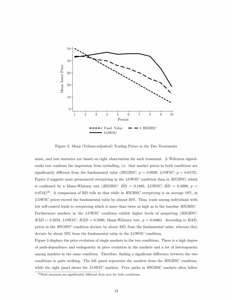
Figure 2 shows how average market prices in LOWSC and HIGHSC evolve over the ten trading
periods. In both conditions, average market prices start out at a similar level, displaying a moderate
level of underpricing. However, from the third period onwards, average prices in both conditions
exceed the fundamental value. Eventually, average market prices drop sharply, but do not drop
below the fundamental value again.
The most conservative comparisons between the two treatments are based on market averages over
all traders and over all ten periods. This is the approach we apply for all non-parametric tests
regarding aggregate market outcomes. These averages are statistically independent in the strict
12
0
10
20
30
40
50
Mean A
sset
Pri
ce
1 2 3 4 5 6 7 8 9 10
Period
Fund. Value HIGHSC
LOWSC
Figure 2: Mean (Volume-adjusted) Trading Prices in the Two Treatments
sense, and test statistics are based on eight observations for each treatment. A Wilcoxon signed-
ranks test confirms the impression from eyeballing, i.e. that market prices in both conditions are
significantly different from the fundamental value (HIGHSC : p = 0.0929, LOWSC : p = 0.0173).
Figure 2 suggests more pronounced overpricing in the LOWSC condition than in HIGHSC, which
is confirmed by a Mann-Whitney test (HIGHSC : RD = 0.1885, LOWSC : RD = 0.4990; p =
0.0742)16. A comparison of RD tells us that while in HIGHSC overpricing is on average 19%, in
LOWSC prices exceed the fundamental value by almost 50%. Thus, trade among individuals with
low self-control leads to overpricing which is more than twice as high as in the baseline HIGHSC.
Furthermore markets in the LOWSC condition exhibit higher levels of mispricing (HIGHSC :
¯RAD = 0.3253, LOWSC : ¯RAD = 0.5890; Mann-Whitney test: p = 0.0460). According to RAD,
prices in the HIGHSC condition deviate by about 33% from the fundamental value, whereas they
deviate by about 59% from the fundamental value in the LOWSC condition.
Figure 3 displays the price evolution of single markets in the two conditions. There is a high degree
of path-dependence and endogeneity in price evolution in the markets and a lot of heterogeneity
among markets in the same condition. Therefore, finding a significant difference between the two
conditions is quite striking. The left panel represents the markets from the HIGHSC condition,
while the right panel shows the LOWSC markets. Price paths in HIGHSC markets often follow
16Both measures are significantly different from zero for both conditions.
13

a rather flat or declining development, while in LOWSC a number of markets display a hump-
shaped price evolution that initially increases and peaks in later trading periods. The emergence of
overpricing can oftentimes be attributed to constant prices despite decreasing fundamental values
(Huber and Kirchler, 2012; Kirchler et al., 2012) – a description that fits price paths in our HIGHSC
markets better than those in LOWSC markets.17
0
10
20
30
40
50
60
70
Mean A
sset
Pri
ce
1 2 3 4 5 6 7 8 9 10
Period
Fund. Value Mean Price
Individual Markets
HIGHSC
0
10
20
30
40
50
60
70
Mean A
sset
Pri
ce
1 2 3 4 5 6 7 8 9 10
Period
Fund. Value Mean Price
Individual Markets
LOWSC
Figure 3: Evolution of Individual Market Prices in HIGHSC and LOWSC
4.4 Potential Transmission Mechanisms of the Treatment Effect
Having established a significant treatment effect, the next step is to look at potential channels via
which self-control variations could have an effect on market outcomes. Detailed descriptive results
on the variables considered in this section can be found in sections A.4ff. of the appendix.
17Section A.1 in the appendix shows a comparison of overpricing measures across treatments for each periodseparately. Overpricing in LOWSC significantly exceeds overpricing in HIGHSC in periods 6-9.
14

4.4.1 Cognitive Abilities and Risk Attitude
Self-control depleted participants might not be willing to think as hard and thus provide the (wrong)
intuitive answers in the CRT. The average number of correct answers in the CRT was 1.05 in
HIGHSC and 1.14 in LOWSC. The difference in CRT score between the two conditions is not
significant according to a Mann-Whitney test (p = 0.7223). We conclude that the Stroop task did
not have an impact on our incentivized version of the CRT.18 Risk attitudes might be affected by
self-control depletion. The average certainty equivalent we elicited is close to the lottery’s expected
value: 2.2 in HIGHSC and 2.15 in LOWSC. Like the literature exploring the effect of reduced
self-control on risk attitude that has come to inconclusive results (e.g. Bruyneel et al., 2009; Unger
and Stahlberg, 2011; Gerhardt et al., 2015), we also find no significant effect (Mann-Whitney test,
p = 0.4083) of our treatment variation on risk attitudes as measured by the multiple price list
certainty equivalent elicitation.
4.4.2 Trading Activity
An additional channel through which our results could be explained is changes in trading activity,
i.e. the number of traded shares per trading period. People low in self-control have been reported
to become more passive (Baumeister et al., 1998, Experiment 4). Increased passivity and thus a
thinner market in LOWSC, where few trades could drive overpricing, could be responsible for our
results. Thus we compare the number of shares traded in the two conditions. Figure 4 illustrates
the evolution of average shares traded per period. Traders in HIGHSC traded slightly more overall:
while the average trader traded 13.02 shares per period in HIGHSC, only 11.39 shares changed
hands on average per trader in each period in LOWSC. However, according to a Mann-Whitney test,
there is no significant difference between amounts traded between the two conditions (p = 0.3446).19
When analyzing the results of Experiment II, we shall take a closer look at trading strategies of
self-control depleted traders versus non-depleted traders.
4.4.3 Regressions Controlling for Potential Channels
Although our control variables seem unaffected by our treatment, they could still possess explana-
tory power for the difference in overpricing that we observe. We therefore run regressions, including
controls as indepedent variables. To avoid endogeneity problems across trading periods and between
subjects, respectively, we aggregate overpricing measures over all periods on the individual level
and use robust standard errors clustered at the market level. We do this separately for sales and
18If we include the observations from our second experiment, the CRT scores of the two groups become 1.0875and 1.1375 respectively with p = 0.7442 from a Mann-Whitney test. Similar results hold for the other tests in thissection.
19An additional regression analysis in Table 7 in appendix A.2 reinforces this conclusion.
15

0
5
10
15
20
Num
ber
of Share
s T
raded
1 2 3 4 5 6 7 8 9 10
Period
HIGHSC LOWSC
Figure 4: Evolution of Average Shares Traded per Trader by Condition
purchases, since selling above fundamental value results in an expected profit, while buying above
fundamental value results in an expected loss. We define measures for individual overpricing for
purchases and sales, which we call IndRDpurchases and IndRDsales, respectively. Similar to the
measure RD they are defined as the percentage of buying (selling) prices exceeding the asset’s fun-
damental value pooled over all periods, but for each subject’s buying (selling) activity separately
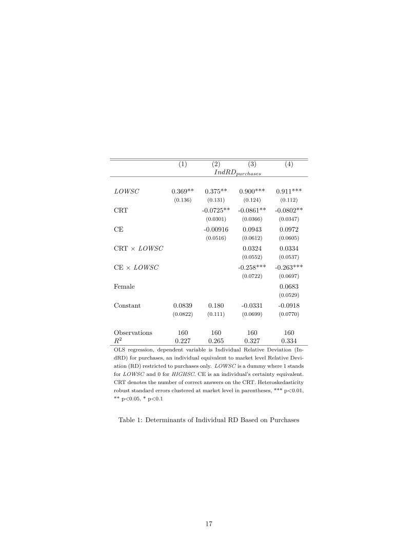
instead of on the market level as before. We report results on IndRDpurchases as the dependent
variable in the regressions in Table 1. In appendix A.2, we provide robustness checks for our chosen
approach for sales and both aggregated sales and purchases.
In all four models we are interested in the effect of the explanatory variables on IndRDpurchases,
our measure of an individual’s overpricing tendency. Throughout all specifications, we observe a
significant treatment effect: Being in LOWSC increases an individual’s propensity to buy at exces-
sive prices. In specification (2), our measure of risk attitude is not significant, but if we also include
interactions with our treatments in specifications (3) and (4), relative risk seeking is correlated with
lower individual overpricing when self-control capabilities are reduced. Performance on the CRT
has the expected effect of reducing the tendency of buying at prices above fundamental value in all
specifications where it is included, and its effect does not significantly differ between participants
in LOWSC and HIGHSC markets. Hence, introducing measures for risk aversion and cognitive
skills and their interactions with our treatments do not reduce the size or significance of the treat-
16
(1) (2) (3) (4)IndRDpurchases
LOWSC 0.369** 0.375** 0.900*** 0.911***(0.136) (0.131) (0.124) (0.112)
CRT -0.0725** -0.0861** -0.0802**(0.0301) (0.0366) (0.0347)
CE -0.00916 0.0943 0.0972(0.0516) (0.0612) (0.0605)
CRT × LOWSC 0.0324 0.0334(0.0552) (0.0537)
CE × LOWSC -0.258*** -0.263***(0.0722) (0.0697)
Female 0.0683(0.0529)
Constant 0.0839 0.180 -0.0331 -0.0918(0.0822) (0.111) (0.0699) (0.0770)
Observations 160 160 160 160R2 0.227 0.265 0.327 0.334OLS regression, dependent variable is Individual Relative Deviation (In-
dRD) for purchases, an individual equivalent to market level Relative Devi-
ation (RD) restricted to purchases only. LOWSC is a dummy where 1 stands
for LOWSC and 0 for HIGHSC. CE is an individual’s certainty equivalent.
CRT denotes the number of correct answers on the CRT. Heteroskedasticity
robust standard errors clustered at market level in parentheses, *** p<0.01,
** p<0.05, * p<0.1
Table 1: Determinants of Individual RD Based on Purchases
17

ment coefficient. We conclude that neither changes in cognitive skills nor in risk preferences after
self-control depletion can explain our main result of excess overpricing after self-control depletion.
5 Experiment II: Mixed Markets
5.1 Motivation and Design
The results reported in section 4 referred to markets, in which either all market participants un-
derwent the tough Stroop task or none of them, i.e. either everyone’s self-control resources had
been reduced or no one’s. In this section we report results from markets, in which only half of
the participants’ self-control resources were depleted. Each market consisted of five participants
randomly assigned to the easy (placebo) Stroop version from the HIGHSC condition and five par-
ticipants randomly assigned to the tough Stroop version from the LOWSC condition. We call this
new condition MIXED and for simplicity refer to traders facing the tough version of the Stroop
task as MIXLO traders and to those facing the easy version of the Stroop task as MIXHI traders.
The motivation for this additional experiment is twofold. First, asset market experiments are zero
sum games and behavior is highly path-dependent and endogenous to market prices, which makes
it technically impossible to analyze differences in behavior resulting from reduced self-control in our
homogeneous markets. Therefore, we wanted a condition in which traders under both conditions
are active at the same time. It allows us to assess differences in trading behavior and performance
between MIXLO traders and MIXHI traders. Second, since in real-world settings – either due
to dispositional differences or due to differential previous demands on self-control resources – it is
likely that individuals high and low in self-control interact, we want so see whether the effect of
reduced self-control observed in LOWSC markets can be replicated with a smaller share of depleted
traders in MIXED markets.
We conducted eight additional sessions with 16 markets in April 2014 and November 2015. In
the last four sessions we added several questions to the experimental questionnaires dealing with
participants’ emotions. We were interested whether our variation of self-control had taken effect
via changes in emotional states. In order to reduce experimenter demand effects and as is common
in experiments analyzing emotions, we confronted subjects with several emotions of which some
were not relevant at all to our question of interest. Apart from the assignment to the respective
version of the Stroop task within a market and the additional questions in the questionnaires of
the last four sessions, the experimental protocol remained exactly the same as in Experiment I.
Experimental participants were not aware of the different versions of the Stroop task, i.e. they were
unaware of the fact that half of the traders performed the tough version and half of the traders the
18

easy version, i.e. they did not know that the market was populated by two types of traders with
regard to self-control abilities.
5.2 Aggregate Price Evolution
0
10
20
30
40
50
Mean A
sset
Pri
ce
1 2 3 4 5 6 7 8 9 10
Period
HIGHSC LOWSC
MIXED
Figure 5: Trading Price Evolution Including MIXED
Figure 5 shows the evolution of average trading prices in all three treatments of Experiment I and
II. Interestingly, the effect of reduced self-control on mispricing and overpricing does not seem to be
changed if only part of the trader population is self-control depleted. Both LOWSC and MIXED
on average display more overpricing than HIGHSC. For MIXED we observe an average RAD of
0.551 and an average RD of 0.430. A Mann-Whitney test confirms that the mispricing measure
RAD in MIXED is significantly different from HIGHSC (p = 0.0500) but cannot be statistically
distinguished from LOWSC (p = 0.8065). This result also holds for our overpricing measure: RD
in MIXED differs significantly from HIGHSC (p = 0.0864), but not from LOWSC (p = 0.5006).20
Figure 6 illustrates the evolution of mean trading prices for the 16 individual markets in the MIXED
condition. Qualitatively, we get similar results as in LOWSC. That is, in some of these markets
prices exhibit a hump-shaped development, initially increasing and peaking in some intermediate
period. Thus already the presence of a moderate share of traders with depleted self-control abilities
20The results of these comparisons also hold when looking at quantity- or trade-adjusted mean prices.
19

0
10
20
30
40
50
60
70
Mean A
sset
Pri
ce
1 2 3 4 5 6 7 8 9 10
Period
Fund. Value Mean Price
Individual Markets
MIXED
Figure 6: Price Evolution in Individual Markets in MIXED
is sufficient to reproduce the excess overpricing we observed when all traders’ self-control levels were
depleted.
5.3 Differences in Trading Behavior and Outcomes
5.3.1 Trading Behavior
Differences in market outcomes in the MIXED condition compared to HIGHSC markets must result
from different actions of MIXLO traders. However, when analyzing trading behavior, distinguishing
cause and effect is particularly difficult, as already mentioned earlier. A particular deviation in
behavior by some traders in the early phases of a market might shift behavior of other (non-depleted)
traders. We therefore start by focusing on the very first trading period, where dependencies are
less relevant than in later periods. Table 2 compares several variables concerning trading activity
between MIXLO and MIXHI traders. Remember that we conduct all statistical tests based on the
most conservative definition of independence (the market level), and hence significant effects are
usually associated with large absolute differences.
According to Wilcoxon signed-rank tests MIXLO traders make significantly lower bids initially
(p = 0.035) and post these bids earlier than their non-depleted peers (p = 0.017). They are also
quicker in posting their first bid at the beginning of the period (p = 0.048). While not significant,
there also seems to be the tendency that MIXLO traders (while bidding low) ask for a higher price
20

Group Mean
MIXHI MIXLO p-value
pbid 36.377 28.487 0.035**pask 49.931 54.478 0.196qbid 16.109 17.788 0.660qask 14.389 15.202 0.796timebid 59.575 73.000 0.017**timeask 69.770 69.617 0.796
firsttimebid 68.483 80.154 0.048**
firsttimeask 85.365 85.565 0.959
Variables starting with a p denote prices, q quantities and time
variables refer to the time remaining in the current period, thus
higher values indicate behavior earlier on. bid and ask refer to
posted bids and asks, p-values from Wilcoxon signed-rank tests
with data collapsed on market and treatment level, *** p<0.01,
** p<0.05, * p<0.1
Table 2: First Period Differences in Trading Behavior
than the MIXHI traders (p = 0.196). After period one, these differences vanish, suggesting that
non-depleted traders start imitating the behavior of self-control depleted traders.21 The averages
in Table 2 suggest an initially stronger speculative motive of MIXLO traders, trying to buy lower
and sell higher than MIXHI traders. From trading period two on, however, their behavior has
incited non-depleted traders to behave similarly and hence set many markets on an entirely different
trajectory.
ρ p-value
pbid 0.436 0.104pask 0.488 0.055*qbid 0.486 0.066*qask -0.229 0.393timebid 0.607 0.016**timeask -0.262 0.327
firsttimebid 0.421 0.118
firsttimeask -0.079 0.770
Rank correlations of average first-period be-
havior over all market participants with av-
erage relative deviation over periods 2-10 for
MIXED markets, *** p<0.01, ** p<0.05, *
p<0.1
Table 3: Rank Correlations of First Period Behavior with Overpricing
Table 3 presents evidence that the observed differences in first period behavior between our treated
and non-treated traders are also those behaviors that are correlated with later overpricing. While
21Results for period two are not reported, but available upon request from the authors.
21

Table 2 has shown that low-self control traders bid earlier in period one and also post their first
bid significantly earlier, Table 3 shows that markets in which bidding occurs early in period one,
are those that exhibit more overpricing over the course of the experiment.
5.3.2 Profits
On average, MIXLO traders earned ¤ 8.16, and MIXHI traders earned ¤ 7.84 on the experimental
asset market – a difference that is not significant (Wilcoxon signed-rank test, p = 0.9794). We
consider this as evidence that inhibited self-control abilities affect overpricing, but that depleted
traders are not necessarily driven out of the market. Instead, as shown previously, they might
goad non-depleted traders into speculative behavior, making everyone end up with similar profits.
While this suggests that a lack of self-control abilities is not necessarily detrimental to trading
performance, it shows how negative the effect can be for markets on which traders potentially
imitate each other’s behavior.
5.4 Increased Emotional Reactivity
In the experimental sessions that we conducted in November 2015, we asked participants a number
of questions relating to their emotional experience during the asset market. In particular, we asked
participants to rate how strongly they felt a number of emotions at the beginning of the first period
and at the end of the last period, respectively. We asked participants to recollect there emotions.22
Table 4 reports the results for those emotions that have previously been connected to overpricing
in experimental asset markets (Andrade et al., 2015; Breaban and Noussair, 2013; Hargreaves Heap
and Zizzo, 2011; Lahav and Meer, 2012). Note that we collapsed all the emotional measures on the
treatment group level within each market and test for differences with Wilcoxon signed-rank tests.
Strikingly, the intensity of every single measure of experienced emotions is higher in the MIXLO
than in the MIXHI group, with many measures being statistically significant. At the beginning of
period 1, MIXLO participants report to feel borderline significantly more surprise (p = 0.103) and
significantly more joy (p = 0.058). Remember that Lahav and Meer (2012) found that inducing
positive mood before trading leads to higher deviations from fundamental values and thus larger
levels of overpricing and that correlational studies also suggest such a relationship (Breaban and
Noussair, 2013; Hargreaves Heap and Zizzo, 2011). Furthermore, at the end of the final trading
period, MIXLO traders report significantly higher levels of excitement, fear and surprise than
MIXHI participants (all p < 0.05).
22We also provided participants with a questionnaire regarding their trading behavior which we do not report here.The average responses to all the emotion-related questions and the test statistics can be found in Table 9 of theappendix. Average values for changes in emotions over time can be found in Table 10.
22

We also asked participants in the post-experimental questionnaire explicitly about how strongly
they felt their behavior was driven by emotions and how much they had tried to suppress the
influence of emotions on their trading behavior. Even though the difference in averages goes in
the expected direction, given the responses to the questions on experienced emotions, they fail to
reach significance on conventional levels. The results indicate that the behavior of the traders with
depleted self-control abilities might have been driven by emotional factors to a larger degree than
they were aware of themselves.
MIXHI MIXLO p-value
Beginning of the first Period
excitement 4.200 4.500 0.400fear 2.100 2.175 0.395surprise 3.600 4.050 0.103joy 3.625 4.375 0.058*
End of the last Period
excitement 3.425 4.200 0.042**fear 1.900 2.575 0.014**surprise 2.450 3.400 0.030**joy 3.375 4.125 0.207
Self-Evaluation of Emotional Reactivity
emotion driven 2.475 2.725 0.362suppressed emotions 5.300 4.950 0.205
Data collapsed on the treatment level per market; responses were on 7 point
Likert scales; test results from Wilcoxon Signed Rank tests; *** p<0.01, **
p<0.05, * p<0.1
Table 4: Ex-post Reported Emotions of Traders in MIXED
5.5 Reduced Cognitive Control
Experiment I did not show a direct effect of the Stroop task on incentivized CRT performance.
Condition MIXED gives us the possibility to look at the issue again, in particular at the association
between CRT, the treatment (MIXLO and MIXHI ), and performance in terms of profits.
Previous research has shown that CRT scores correlate positively with individual participants’
profits in similar experiments (Corgnet et al., 2014; Noussair et al., 2014). Toplak et al. (2011)
find that CRT scores are correlated with measures of cognitive ability, thinking disposition and
executive functioning. Thus, we can interpret the CRT score as a measure of cognitive control. In
order to check whether the effect of CRT performance on profits is similar here, we ran additional
regressions which we report in table 5. Note that we excluded participants who had indicated that
they knew at least one of the CRT questions at the end of the experiment. The knowledge of
23
CRT questions before the experiment might have driven up correct CRT responses and might thus
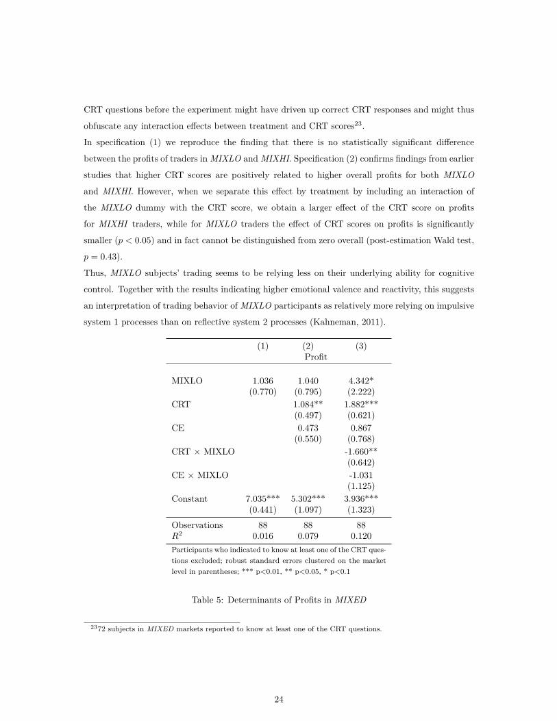
obfuscate any interaction effects between treatment and CRT scores23.
In specification (1) we reproduce the finding that there is no statistically significant difference
between the profits of traders in MIXLO and MIXHI. Specification (2) confirms findings from earlier
studies that higher CRT scores are positively related to higher overall profits for both MIXLO
and MIXHI. However, when we separate this effect by treatment by including an interaction of
the MIXLO dummy with the CRT score, we obtain a larger effect of the CRT score on profits
for MIXHI traders, while for MIXLO traders the effect of CRT scores on profits is significantly
smaller (p < 0.05) and in fact cannot be distinguished from zero overall (post-estimation Wald test,
p = 0.43).
Thus, MIXLO subjects’ trading seems to be relying less on their underlying ability for cognitive
control. Together with the results indicating higher emotional valence and reactivity, this suggests
an interpretation of trading behavior of MIXLO participants as relatively more relying on impulsive
system 1 processes than on reflective system 2 processes (Kahneman, 2011).
(1) (2) (3)Profit
MIXLO 1.036 1.040 4.342*(0.770) (0.795) (2.222)
CRT 1.084** 1.882***(0.497) (0.621)
CE 0.473 0.867(0.550) (0.768)
CRT × MIXLO -1.660**(0.642)
CE × MIXLO -1.031(1.125)
Constant 7.035*** 5.302*** 3.936***(0.441) (1.097) (1.323)
Observations 88 88 88R2 0.016 0.079 0.120
Participants who indicated to know at least one of the CRT ques-
tions excluded; robust standard errors clustered on the market
level in parentheses; *** p<0.01, ** p<0.05, * p<0.1
Table 5: Determinants of Profits in MIXED
2372 subjects in MIXED markets reported to know at least one of the CRT questions.
24

6 Discussion
We observe a strong main effect of self-control depletion on overpricing in both experiments. The
difference in overpricing cannot be explained by a change in risk attitudes or a simple change in
cognitive abilities. Experiment II gives us additional ways to assess potential explanations for the
excess overpricing after self-control depletion.
First, there are differences in trading behavior. Self-control depleted traders trade slightly less,
and their initial trading behavior shows patterns of speculative trading. For instance, the fact that
self-control depleted traders post bids significantly earlier supports the notion that their behavior is
driven by a higher degree of impulsivity than the behavior of non-depleted traders. In an environ-
ment in which early activity and speculation is potentially imitated by others on the market, not
much is needed to set a market on an overpricing trajectory. Notably, trading behavior is strongly
path-dependent in experimental asset markets, and the evolution of prices follow different forms
and different timings on different markets. We could have presented additional empirical evidence
for effects of self-control depletion on trading behavior and trading strategies, but such evidence
requires assumptions that are somewhat arbitrary. Hence, we decided to present fewer analyses and
only those in whose robustness we are confident.
Second, there are differences in the reported intensity of emotions and relevance of emotions. Various
studies stress the relevance of pre-market emotional states for market outcomes (Hargreaves Heap
and Zizzo, 2011; Lahav and Meer, 2012; Andrade et al., 2015; Breaban and Noussair, 2013). Lahav
and Meer (2012) and Andrade et al. (2015) found that positivity and excitement respectively induce
more pronounced overpricing in experimental asset markets. Due to these findings, initial differences
before the opening of the asset market (and after the Stroop task) are one channel via which depleted
self-control could have affected overpricing. Apart from the pre-market emotional state, differential
emotional reactions during the market could be driving our results. Emotion regulation has been
shown to draw on self-control resources (Baumeister et al., 1998; Hagger et al., 2010). We have
evidence that participants displayed more intense emotional states, in particular at the end of the
asset market. Even though our experimental design does not allow us to fully rule out a direct effect
of the self-control manipulation on emotional states before the opening of the asset market, given
the result in previous studies of no impact of such manipulations on affect (Baumeister et al., 1998;
Bruyneel et al., 2006; Hagger et al., 2010), the interpretation of the Stroop task resulting in initial
differences in emotional states seems somewhat far-fetched. We thus interpret our treatment effect
as the result of an increased sensitivity towards emotions triggered by self-control depletion. Our
effect is in line with the literature on self-control depletion. For example, Bruyneel et al. (2006) have
shown that people whose self-control has been reduced rely more on affective and less on cognitive
25

features in product choice. Similarly, in our setting traders with low self-control levels could rely
more heavily on affective features of the asset, e.g. the thrill from its recent price increase or from
speculation, than on cognitive features, e.g. the knowledge that the fundamental value of the stock
is decreasing. Thus emotional responses could be responsible for more myopic decision making, a
higher level of overconfidence/overoptimism (Michailova and Schmidt, 2016) and more speculative
trading.
Third, cognitive abilities could be different after the two versions of the Stroop task. However,
the issue is not as straightforward as we expected. For our sample, we cannot provide evidence
on a direct impact of the treatment on CRT performance. This might be because the monetary
incentives to do well in the CRT are relatively high, and it is well-known that people can temporarily
overcome self-control problems if the motivation is sufficient (Muraven and Slessareva, 2003; Vohs
et al., 2012). However, there is evidence in our data for an indirect effect of self-control depletion
on cognitive abilities. We find that the CRT carries predictive power for traders’ profits, but only
if their self-control has not been depleted previously.
There are additional explanations that we cannot pin down fully and have to leave for verification
in future research. Self-control depleted traders, for instance, report significantly higher levels
of surprise after the last period of the market. This could be an indication for a reinforcement of
myopic behavior when being self-control depleted. Another candidate explanation for our treatment
effect is a problem to stop, i.e. to sell early enough and not to stick too long to the expectation of
a future price rise. Self-control depletion could lead to a reluctance to sell an asset whose price is
rising. Similarly, it could lead to undue overoptimism.
7 Conclusion
In this paper, we provide causal empirical evidence for the notion that a lack of self-control can
fuel overpricing on asset markets. We consider experimental continuous double auction markets
for which Smith et al. (1988) first reported a tendency for overpricing. We exogenously reduce
market participants’ ability to exert self-control using a tough version of the Stroop task, which
has previously been shown to deplete people’s ability to exert self-control in subsequent tasks
(Baumeister et al., 1998). Comparing two market settings in which either everyone’s or no one’s
self-control was reduced, we observe significantly more mispricing and overpricing as the result of
a reduction in self-control abilities than without this reduction.
Self-control depletion affects trading behavior and the perception of the trades and market outcomes.
We provide evidence that in markets populated by self-control depleted and non-depleted traders
initial trading strategies of the former show more signs of speculative behavior than of the latter.
26

However, the evidence is not entirely conclusive. Trading is path-dependent on experimental asset
markets, and it is difficult to pin down the exact reasons for overpricing to emerge without making
arbitrary assumptions. We do not observe a performance difference between traders with depleted
self-control and traders with full self-control abilities, suggesting that low self-control traders might
not be driven out of the market, but rather incite other traders to engage in speculative trading.
In addition, we have evidence for an emotional channel that explains our main result. Self-control
depleted traders show stronger emotions, in general, but in particular stronger emotions that have
been linked to overpricing in previous studies that induce emotions or that measure emotions while
trading. Finally, we find that our measure for cognitive skills loses predictive power for the profits
of low self-control traders. This might indicate that even though cognitive skills seem unaffected
by self-control depletion (as are risk attitudes), different cognitive processes play a role in traders
with low self-control levels. These results are in line with a dual systems perspective of self-control:
self-control depleted participants seem to have acted more on the basis of emotions and less on the
basis of cognition, thus driving up prices.
Our findings have relevant implications: First, with differences in self-control levels, we add a
potentially important explanation to the existing explanations for overpricing on asset markets. We
have shown that already a moderate number of participants with low self-control levels are sufficient
to nearly double the extent of overpricing. Second, our results can be regarded as indicative of the
role of self-control in real world markets – here both temporary reductions in self-control as well as
the personality trait self-control might play an important role in determining trading behavior and
perception. Self-control might also be an important attribute on which individuals self-select into
trading. However, low self-control traders might not be as easily exploitable by high self-control
traders as one would think. In our case, they would not have been driven out of the market quickly.
Several practical implications of our results for real-world investing and trading activities come
to mind. Given our findings, investment decisions should not be taken under limited self-control
or willpower conditions. For instance, cognitive load, food or sleep deprivation, and self-control
effort in unrelated domains have been shown to be correlated with limited self-control abilities. If
such conditions are unavoidable, decision aides to sustain self-control such as commitment devices
should prove useful to circumvent the potentially negative consequences. This might be particularly
relevant in fast-paced markets.
Our experiment opens up interesting paths for future research: It would be interesting to see to what
extent our results are robust to changes in alternative market mechanisms such as call markets and
to changes in the fundamental value process such as a constant fundamental value process, which
has been shown to reduce overpricing (Kirchler et al., 2012). Finally, the role of self-control for
27

traders in real markets remains largely unexplored. One can imagine field experiments or using
quasi-experimental variations of self-control abilities to study decisions of traders on real markets.
28

References
Achtziger, A., Alos-Ferrer, C., and Wagner, A. K. (2015). Money, depletion, and prosociality in the
dictator game. Journal of Neuroscience, Psychology, and Economics, forthcoming.
Achtziger, A., Alos-Ferrer, C., and Wagner, A. K. (2016). The impact of self-control depletion on
social preferences in the ultimatum game. Journal of Economic Psychology, 53:1–16.
Ameriks, J., Caplin, A., and Leahy, J. (2003). Wealth accumulation and the propensity to plan.
Quarterly Journal of Economics, 118(3):1007–1047.
Ameriks, J., Caplin, A., Leahy, J., and Tyler, T. (2007). Measuring self-control problems. American
Economic Review, 97(3):966–972.
Andrade, E. B., Odean, T., and Lin, S. (2015). Bubbling with excitement: An experiment. Review
of Finance, forthcoming.
Baumeister, R. F., Bratslavsky, E., Muraven, M., and Tice, D. M. (1998). Ego depletion: Is the
active self a limited resource? Journal of Personality and Social Psychology, 74(5):1252–1265.
Beshears, J., Choi, J. J., Harris, C., Laibson, D., C., M. B., and Sakong, J. (2015). Self control
and commitment: Can decreasing the liquidity of a savings account increase deposits? Working
Paper.
Bosch-Rosa, C., Meissner, T., and Bosch-Domenech, A. (2015). Cognitive bubbles. Working Paper.
Branas-Garza, P., Garcıa-Munoz, T., and Gonzalez, R. H. (2012). Cognitive effort in the beauty
contest game. Journal of Economic Behavior & Organization, 83(2):254–260.
Breaban, A. and Noussair, C. N. (2013). Emotional state and market behavior. Working Paper.
Bruyneel, S., Dewitte, S., Vohs, K. D., and Warlop, L. (2006). Repeated choosing increases suscep-
tibility to affective product features. International Journal of Research in Marketing, 23(2):215–
225.
Bruyneel, S. D., Dewitte, S., Franses, P. H., and Dekimpe, M. G. (2009). I felt low and my purse
feels light: Depleting mood regulation attempts affect risk decision making. Journal of Behavioral
Decision Making, 22(2):153–170.
Bucciol, A., Houser, D., and Piovesan, M. (2011). Temptation and productivity: A field experiment
with children. Journal of Economic Behavior & Organization, 78(1):126–136.
Bucciol, A., Houser, D., and Piovesan, M. (2013). Temptation at work. PloS one, 8(1).
29
Corgnet, B., Hernan-Gonzalez, R., Kujal, P., and Porter, D. (2014). The effect of earned versus
house money on price bubble formation in experimental asset markets. Review of Finance,
19(4):1–34.
De Haan, T. and Van Veldhuizen, R. (2015). Willpower depletion and framing effects. Journal of
Economic Behavior & Organization, 117:47–61.
Dohmen, T., Falk, A., Huffman, D., Sunde, U., Schupp, J., and Wagner, G. G. (2011). Individ-
ual risk attitudes: Measurement, determinants, and behavioral consequences. Journal of the
European Economic Association, 9(3):522–550.
Eckel, C. C. and Fullbrunn, S. C. (2015). Thar “she” blows? gender, competition, and bubbles in
experimental asset markets. American Economic Review, 105(2):906–920.
Fellner, G. and Maciejovsky, B. (2007). Risk attitude and market behavior: Evidence from experi-
mental asset markets. Journal of Economic Psychology, 28(3):338–350.
Fenton-O’Creevy, M., Soane, E., Nicholson, N., and Willman, P. (2011). Thinking, feeling and
deciding: The influence of emotions on the decision making and performance of traders. Journal
of Organizational Behavior, 32(8):1044–1061.
Fischbacher, U. (2007). z-Tree: Zurich toolbox for ready-made economic experiments. Experimental
Economics, 10(2):171–178.
Frederick, S. (2005). Cognitive reflection and decision making. Journal of Economic Perspectives,
19(4):25–42.
Freeman, N. and Muraven, M. (2010). Self-control depletion leads to increased risk taking. Social
Psychological and Personality Science, 1(2):175–181.
Friehe, T. and Schildberg-Horisch, H. (2014). Crime and self-control revisited: Disentangling the
effect of self-control on risk and social preferences. Working Paper.
Fudenberg, D. and Levine, D. K. (2006). A dual-self model of impulse control. American Economic
Review, 96(5):1449–1476.
Gailliot, M. T., Gitter, S. A., Baker, M. D., Baumeister, R. F., et al. (2012). Breaking the rules:
Low trait or state self-control increases social norm violations. Psychology, 3(12):1074–1083.
Gathergood, J. (2012). Self-control, financial literacy and consumer over-indebtedness. Journal of
Economic Psychology, 33(3):590–602.
30

Gerhardt, H., Schildberg-Horisch, H., and Willrodt, J. (2015). Does self-control depletion affect
risk attitudes? Working Paper.
Greiner, B. (2015). Subject pool recruitment procedures: Organizing experiments with orsee.
Journal of the Economic Science Association, 1(1):114–125.
Hagger, M. S., Wood, C., Stiff, C., and Chatzisarantis, N. L. (2010). Ego depletion and the strength
model of self-control: A meta-analysis. Psychological Bulletin, 136(4):495–525.
Hargreaves Heap, S. and Zizzo, D. (2011). Emotions and chat in a financial markets experiment.
Working Paper.
Hofmann, W., Friese, M., and Strack, F. (2009). Impulse and self-control from a dual-systems
perspective. Perspectives on Psychological Science, 4(2):162–176.
Huber, J. and Kirchler, M. (2012). The impact of instructions and procedure on reducing confusion
and bubbles in experimental asset markets. Experimental Economics, 15(1):89–105.
Inzlicht, M. and Schmeichel, B. J. (2012). What is ego depletion? Toward a mechanistic revision
of the resource model of self-control. Perspectives on Psychological Science, 7(5):450–463.
Kahneman, D. (2011). Thinking, fast and slow. Macmillan.
Keynes, J. M. (1936). The general theory of interest, employment and money. Macmillan.
Kirchler, M., Huber, J., and Stockl, T. (2012). Thar she bursts: Reducing confusion reduces
bubbles. American Economic Review, 102(2):865–883.
Kostek, J. and Ashrafioun, L. (2014). Tired winners: The effects of cognitive resources and prior
winning on risky decision making. Journal of Gambling Studies, 30(2):423–434.
Kotabe, H. P. and Hofmann, W. (2015). On integrating the components of self-control. Perspectives
on Psychological Science, 10(5):618–638.
Lahav, Y. and Meer, S. (2012). The effect of induced mood on prices in asset markets – experimental
evidence. Working Paper.
Lo, A. W., Repin, D. V., and Steenbarger, B. N. (2005). Fear and greed in financial markets: A
clinical study of day-traders. American Economic Review, 95(2):352–359.
MacLeod, C. M. (1991). Half a century of research on the stroop effect: An integrative review.
Psychological Bulletin, 109(2):163–203.
31

Martinsson, P., Myrseth, K. O. R., and Wollbrant, C. (2014). Social dilemmas: When self-control
benefits cooperation. Journal of Economic Psychology, 45:213–236.
Masatlioglu, Y., Nakajima, D., and Ozdenoren, E. (2014). Revealed willpower. Working Paper.
Michailova, J. and Schmidt, U. (2016). Overconfidence and bubbles in experimental asset markets.
Working Paper.
Miller, R. M. (2002). Can markets learn to avoid bubbles? Journal of Psychology and Financial
Markets, 3(1):44–52.
Muraven, M. (2010). Building self-control strength: Practicing self-control leads to improved self-
control performance. Journal of Experimental Social Psychology, 46(2):465–468.
Muraven, M. and Baumeister, R. F. (2000). Self-regulation and depletion of limited resources: Does
self-control resemble a muscle? Psychological Bulletin, 126(2):247–259.
Muraven, M., Baumeister, R. F., and Tice, D. M. (1999). Longitudinal improvement of self-
regulation through practice: Building self-control strength through repeated exercise. Journal of
Social Psychology, 139(4):446–457.
Muraven, M. and Slessareva, E. (2003). Mechanisms of self-control failure: Motivation and limited
resources. Personality and Social Psychology Bulletin, 29(7):894–906.
Nadler, A., Jiao, P., Alexander, V., Johnson, C., and Zak, P. (2015). Testosterone and trading: A
biological driver of asset mispricing. Working Paper.
Noussair, C. N. and Tucker, S. (2013). Experimental research on asset pricing. Journal of Economic
Surveys, 27(3):554–569.
Noussair, C. N., Tucker, S. J., and Xu, Y. (2014). A futures market reduces bubbles but allows
greater profit for more sophisticated traders. Working Paper.
Ozdenoren, E., Salant, S. W., and Silverman, D. (2012). Willpower and the optimal control of
visceral urges. Journal of the European Economic Association, 10(2):342–368.
Palan, S. (2013). A review of bubbles and crashes in experimental asset markets. Journal of
Economic Surveys, 27(3):570–588.
Petersen, G.-K., Spickers, T., Glaser, M., and Brodbeck, F. C. (2015). How private investors’ stress
influences investor behavior and financial markets. Conference Experimental Finance.
Porter, D. P. and Smith, V. L. (1995). Futures contracting and dividend uncertainty in experimental
asset markets. Journal of Business, 68(4):509–541.
32

Schmeichel, B. J., Vohs, K. D., and Baumeister, R. F. (2003). Intellectual performance and ego
depletion: Role of the self in logical reasoning and other information processing. Journal of
Personality and Social Psychology, 85(1):33–46.
Schmeichel, B. J. and Zell, A. (2007). Trait self-control predicts performance on behavioral tests of
self-control. Journal of Personality, 75(4):743–756.
Smith, A., Lohrenz, T., King, J., Montague, P. R., and Camerer, C. F. (2014). Irrational exuberance
and neural crash warning signals during endogenous experimental market bubbles. Proceedings
of the National Academy of Sciences, 111(29):10503–10508.
Smith, V. L., Suchanek, G. L., and Williams, A. W. (1988). Bubbles, crashes, and endogenous
expectations in experimental spot asset markets. Econometrica, 56(5):1119–1151.
Stockl, T., Huber, J., and Kirchler, M. (2010). Bubble measures in experimental asset markets.
Experimental Economics, 13(3):284–298.
Stojic, H., Anreiter, M. R., and Martinez, J. A. C. (2013). An experimental test of the dual self
model. Working Paper.
Stroop, J. R. (1935). Studies of interference in serial verbal reactions. Journal of Experimental
Psychology, 18(6):643–662.
Tangney, J. P., Baumeister, R. F., and Boone, A. L. (2004). High self-control predicts good
adjustment, less pathology, better grades, and interpersonal success. Journal of Personality,
72(2):271–324.
Thaler, R. H. and Shefrin, H. M. (1981). An economic theory of self-control. Journal of Political
Economy, 89(2):392–406.
Tice, D. M. and Bratslavsky, E. (2000). Giving in to feel good: The place of emotion regulation in
the context of general self-control. Psychological Inquiry, 11(3):149–159.
Toplak, M. E., West, R. F., and Stanovich, K. E. (2011). The cognitive reflection test as a predictor
of performance on heuristics-and-biases tasks. Memory & Cognition, 39(7):1275–1289.
Unger, A. and Stahlberg, D. (2011). Ego-depletion and risk behavior: Too exhausted to take a risk.
Social Psychology, 42(1):28–38.
Vohs, K. D., Baumeister, R. F., and Schmeichel, B. J. (2012). Motivation, personal beliefs, and lim-
ited resources all contribute to self-control. Journal of Experimental Social Psychology, 48(4):943–
947.
33

A Appendix – will be provided online
A.1 Period-specific Price Comparisons
Looking at single periods, it is possible to get a more precise picture of when the price differences
between conditions arise. Table 6 reports the per-period differences of volume-adjusted mean prices,
trade-adjusted mean prices, RAD and RD between LOWSC and HIGHSC. The z-values from Mann-
Whitney tests testing the equality of the respective measures across the two conditions are displayed
in parentheses with significance levels indicated by asterisks. While in the first periods we see almost
no price differences, starting from period five, markets in LOWSC exhibit significantly higher mean
prices, mispricing, and overpricing, with the peak in period 8. There are no significant differences
between the two conditions in the ultimate period. By definition, this implies a more pronounced
bubble and burst pattern in LOWSC markets than in HIGHSC markets.
34

Period∆volume-adjusted ∆trade-adjusted
∆RAD ∆RDmean price mean price
1-0.67 -0.85 0.0143 -0.0245
(0.84) (0.735) (-0.63) (0.84)
20.73 2.87 -0.0749 0.0266
(0.105) (-0.21) (0.21) (0.105)
34.53 3.38 0.0006 0.1646
(-0.84) (-0.525) (-0.105) (-0.84)
47.18 7.64 * 0.1720 0.2612
(-1.47) (-1.89) (-1.26) (-1.47)
59.24 * 9.03 * 0.2523 0.3359 *
(-1.785) (-1.785) (-1.47) (-1.785)
612.27 ** 12.01 ** 0.4186 ** 0.4461 **
(-2.205) (-2.31) (-2.205) (-2.205)
715.90 ** 15.84 ** 0.5703 ** 0.5781 **
(-2.521) (-2.415) (-2.521) (-2.521)
818.40 ** 19.00 ** 0.6573 ** 0.6693 **
(-2.521) (-2.521) (-2.521) (-2.521)
911.69 ** 11.78 ** 0.4249 ** 0.4249 **
(-2.1) (-1.995) (-2.1) (-2.1)
106.13 6.48 0.2007 0.2228
(-1.26) (-1.26) (-1.05) (-1.26)
Differences between LOWSC and HIGHSC and z-values (in parentheses) for Mann-
Whitney tests. Volume-adjusted mean prices denote the average price per asset, while
trade-adjusted mean prices denote average price per trade.
* p < 0.1, ** p < 0.05, *** p < 0.01
Table 6: Period-specific Effects
35

A.2 Additional Regression Results
(1) (2) (3) (4)
average quantity traded
LOWSC -1.636 -1.643 -3.030 -3.019
(1.646) (1.666) (3.551) (3.658)
CRT 0.0705 -0.00550 0.000201
(0.566) (0.979) (1.010)
CE -0.0157 -0.248 -0.245
(0.752) (0.813) (0.839)
CRT × LOWSC 0.118 0.119
(1.172) (1.173)
CE × LOWSC 0.581 0.576
(1.605) (1.658)
female 0.0667
(1.479)
Constant 13.02*** 12.98*** 13.57*** 13.51***
(0.750) (1.674) (1.454) (2.318)
Observations 160 160 160 160
R2 0.012 0.012 0.013 0.013
OLS regression, dependent variable is individual average number of trades.
LOWSC is a dummy where 1 stands for LOWSC and 0 for HIGHSC. CE
is an individual’s certainty equivalent. CRT denotes the number of correct
answers on the CRT. Heteroskedasticity robust standard errors clustered at
market level in parentheses, *** p<0.01, ** p<0.05, * p<0.1
Table 7: Determinants of Trading Activity
36

(1) (2) (3) (4) (5)
average quantity traded
MIXLO -2.230 -2.049 -2.343 -1.548 -1.259
(1.606) (2.620) (1.644) (2.686) (4.213)
RD 2.234 2.445 1.240 2.110 2.334
(3.427) (5.882) (3.733) (6.000) (6.111)
RD × MIXEDLO -0.421 -1.863 -2.997
(5.362) (5.428) (5.744)
CRT -0.731 -0.776 -0.217
(0.600) (0.553) (0.869)
CE 1.522** 1.617** 1.332
(0.677) (0.719) (0.894)
CRT × MIXEDLO -1.217
(1.534)
CE × MIXEDLO 0.752
(1.546)
Constant 12.27*** 12.18*** 10.41*** 9.891*** 9.749***
(1.850) (2.648) (1.653) (2.952) (3.120)
Observations 160 160 160 160 160
R2 0.027 0.027 0.046 0.047 0.052
OLS regression, dependent variable is individual average number of trades. MIXLO is a
dummy where 1 stands for MIXLO and 0 for MIXHI. CE is an individual’s certainty equiv-
alent. CRT denotes the number of correct answers on the CRT. Heteroskedasticity robust
standard errors clustered at market level in parentheses, *** p<0.01, ** p<0.05, * p<0.1
Table 8: Determinants of Trading Activity (MIXED)
37

MIXHI MIXLO p-value
excitement1 4.200 4.500 0.400
fear1 2.100 2.175 0.395
surprise1 3.600 4.050 0.103
anger1 1.800 2.025 0.440
relief1 2.825 3.250 0.161
sadness1 1.525 1.725 0.324
joy1 3.625 4.375 0.058*
excitement2 3.425 4.200 0.042**
fear2 1.900 2.575 0.014**
surprise2 2.450 3.400 0.030**
anger2 2.025 2.000 0.723
relief2 3.275 4.150 0.233
sadness2 1.950 1.725 0.622
joy2 3.375 4.125 0.207
emotion intensity 2.720 3.163 0.025**
emotion valence 1.464 1.969 0.208
emotion intensity1 2.811 3.157 0.123
emotion valence1 1.754 2.069 0.123
emotion intensity2 2.629 3.168 0.025**
emotion valence2 1.604 1.944 0.400
Note: p-values from Wilcoxon-Signed Rank tests collapsing data on
the market level by MIXLO and MIXHI respectively; emotion inten-
sity is the average score over all emotion questions, emotion valence is
the average score over all positive emotions minus the negative score
over all negative emotions; variables ending in 1 or 2 relate to questions
relating to the beginning or the end of the stock market respectively;
*** p<0.01, ** p<0.05, * p<0.1
Table 9: Ratings of Emotions in MIXED Markets
38

MIXHI MIXLO p-value
diff excitement -0.775 -0.300 0.232
diff fear -0.200 0.400 0.029**
diff surprise -1.150 -0.650 0.288
diff anger 0.225 -0.025 0.575
diff relief 0.450 0.900 0.441
diff sadness 0.425 0.000 0.290
diff joy -0.250 -0.250 1.000
Note: p-values from Wilcoxon-Signed Rank tests collapsing data on
the market level by MIXLO and MIXHI respectively; *** p<0.01, **
p<0.05, * p<0.1
Table 10: Changes of ex-post Emotion Ratings in MIXED Markets
39

(1) (2) (3) (4)
IndRDsales
LOWSC 0.326** 0.326** 0.596** 0.607**
(0.147) (0.147) (0.230) (0.218)
CRT -0.00262 -0.0346 -0.0290
(0.0289) (0.0431) (0.0437)
CE 0.0121 0.0745 0.0773
(0.0459) (0.0526) (0.0535)
CRT × LOWSC 0.0620 0.0630
(0.0557) (0.0550)
CE × LOWSC -0.156* -0.160*
(0.0841) (0.0810)
Female 0.0655
(0.0472)
Constant 0.193* 0.169 0.0654 0.00916
(0.103) (0.128) (0.0850) (0.0939)
Observations 160 160 160 160
R2 0.188 0.188 0.216 0.222
OLS regression, dependent variable is Individual Relative Deviation
(IndRD) for sales, an individual equivalent to market level Relative
Deviation (RD) restricted to sales only. LOWSC is a dummy where 1
stands for LOWSC and 0 for HIGHSC. CE is an individual’s certainty
equivalent. CRT denotes the number of correct answers on the CRT.
Heteroskedasticity robust standard errors clustered at market level in
parentheses, *** p<0.01, ** p<0.05, * p<0.1
Table 11: Determinants of individual RD based on sales
40

(1) (2) (3) (4)
IndRD
LOWSC 0.357** 0.361** 0.760*** 0.771***
(0.137) (0.134) (0.150) (0.138)
CRT -0.0448* -0.0614 -0.0557
(0.0244) (0.0361) (0.0353)
CE -0.00420 0.0768 0.0796
(0.0445) (0.0511) (0.0510)
CRT × LOWSC 0.0361 0.0370
(0.0465) (0.0455)
CE × LOWSC -0.202*** -0.207***
(0.0674) (0.0646)
Female 0.0665*
(0.0366)
Constant 0.121 0.177 0.0160 -0.0411
(0.0879) (0.109) (0.0651) (0.0672)
Observations 160 160 160 160
R2 0.265 0.282 0.330 0.338
OLS regression, dependent variable is Individual Relative Deviation (In-
dRD), an individual equivalent to market level Relative Deviation (RD).
LOWSC is a dummy where 1 stands for LOWSC and 0 for HIGHSC. CE
is an individual’s certainty equivalent. CRT denotes the number of correct
answers on the CRT. Heteroskedasticity robust standard errors clustered at
market level in parentheses, *** p<0.01, ** p<0.05, * p<0.1
Table 12: Correlates of Individual Miscpricing
41

(1) (2) (3) (4) (5)
Trading Profits
MIXLO 0.204 0.760 0.153 0.527 3.404**
(0.443) (0.522) (0.392) (0.488) (1.525)
RD 0.660 0.768** 1.178 1.357*
(0.721) (0.298) (0.676) (0.734)
RD × MIXLO -1.293 -0.877 -1.249
(1.436) (1.360) (1.426)
CRT 1.376*** 1.355*** 1.834***
(0.239) (0.241) (0.395)
CE 0.423 0.468 0.844
(0.486) (0.483) (0.577)
CRT × MIXLO -0.975
(0.632)
CE × MIXLO -0.774
(0.867)
Constant -0.101 -0.384 -2.846** -3.089** -4.474***
(0.223) (0.261) (1.025) (1.054) (1.209)
Observations 160 160 160 160 160
R2 0.001 0.005 0.156 0.158 0.184
OLS regression, dependent variable is average trading profit from asset market
in ¤ RD is the average Relative Deviation in a market, RD×LOWSC is the
interaction of RD and a dummy that equals one, if the subject is assigned to the
hard version of the Stroop task. CRT denotes the number of correct answers in the
CRT, CE is the individual certainty equivalent, robust standard errors clustered
on market level in parentheses, *** p<0.01, ** p<0.05, * p<0.1
Table 13: Determinants of Trading Profits
42

A.3 Distribution of Answers in the Stroop Task
0
.1
.2
.3
0 100 200 300 0 100 200 300
HIGHSC LOWSCFra
ctio
n
Stroop Task: Number of Correct Answers
Figure 7: Correct Stroop responses in HIGHSC vs. LOWSC
0
.1
.2
100 150 200 250 100 150 200 250
HIGHSC LOWSC
Fra
ctio
n
Stroop Task: Number of Trials
Figure 8: Stroop trials in HIGHSC vs. LOWSC
43

0
.2
.4
.6
.8
0 5 10 15 20 0 5 10 15 20
HIGHSC LOWSC
Fra
ctio
n
Stroop Task: Number of Errors
Figure 9: Errors in the Stroop task in HIGHSC vs. LOWSC
Distribution of Answers in the Stroop Task
HIGHSC mean standard deviation
Correct Answers 192.65 22.6146
Trials 194.55 23.55973
Errors 1.9 1.879941
LOWSC mean standard deviation
Correct Answers 171.3125 20.68363
Trials 174.45 20.96948
Errors 3.14 2.971356
Table 14: Distribution of Answers in the Stroop Task
44
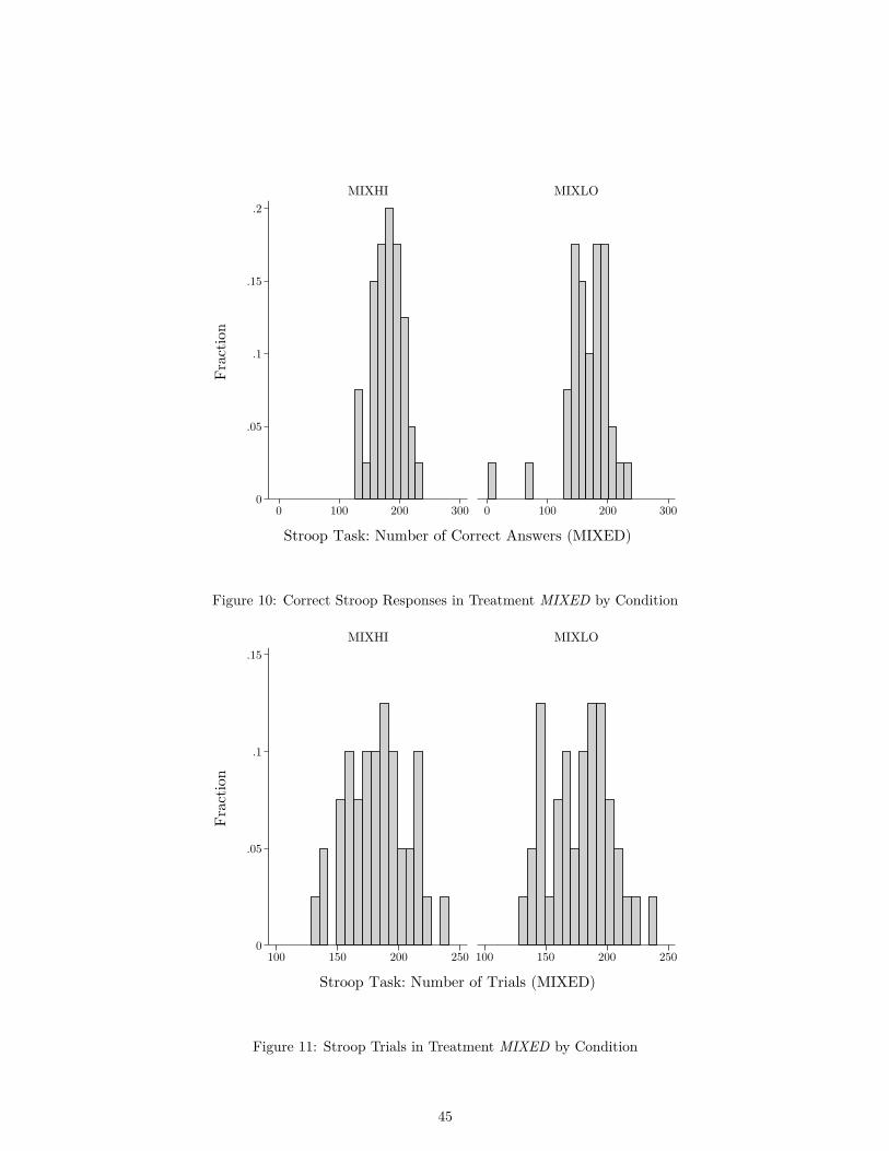
0
.05
.1
.15
.2
0 100 200 300 0 100 200 300
MIXHI MIXLO
Fra
ctio
n
Stroop Task: Number of Correct Answers (MIXED)
Figure 10: Correct Stroop Responses in Treatment MIXED by Condition
0
.05
.1
.15
100 150 200 250 100 150 200 250
MIXHI MIXLO
Fra
ctio
n
Stroop Task: Number of Trials (MIXED)
Figure 11: Stroop Trials in Treatment MIXED by Condition
45

0
.2
.4
.6
.8
0 5 10 15 20 0 5 10 15 20
MIXHI MIXLO
Fra
ctio
n
Stroop Task: Number of Errors (MIXED)
Figure 12: Errors in the Stroop Task in Treatment MIXED by condition24
24Two outliers were dropped from this display in the MIXLO group, both of whom apparently did not fullyunderstand the task. One had 123 errors and the other had 205 errors.
46

Distribution of Answers in the Stroop Task (MIXED)
HIGHSC mean standard deviation
Correct Answers 179.225 24.1135
Trials 182.65 24.59784
Errors 2.425 1.448031
LOWSC mean standard deviation
Correct Answers 164.05 39.93838
Trials 178.3 25.47518
Errors 13.25 36.44367
Table 15: Distribution of Answers in the Stroop Task (MIXED)
A.4 Distribution of Subjective Measures
0
.1
.2
.3
.4
1 2 3 4 5 1 2 3 4 5
HIGHSC LOWSC
Fra
ction
Strain
Figure 13: Strain in HIGHSC vs. LOWSC
47
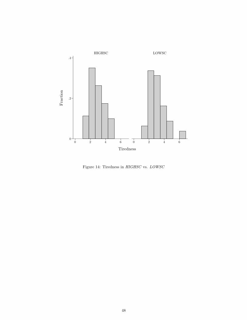
0
.2
.4
0 2 4 6 0 2 4 6
HIGHSC LOWSC
Fra
ctio
n
Tiredness
Figure 14: Tiredness in HIGHSC vs. LOWSC
48

Distribution of Subjective Measures
HIGHSC mean standard deviation
Strain 2.6375 0.9839696
Tiredness 2.8 1.162712
LOWSC mean standard deviation
Strain 3.175 0.9907803
Tiredness 2.9875 1.206457
Table 16: Distribution of Subjective Measures
0
.1
.2
.3
.4
1 2 3 4 5 1 2 3 4 5
MIXHI MIXLO
Fra
ctio
n
Strain (MIXED)
Figure 15: Strain in Treatment MIXED by Condition
49

0
.2
.4
0 2 4 6 0 2 4 6
MIXHI MIXLO
Fra
ctio
n
Tiredness (MIXED)
Figure 16: Tiredness in Treatment MIXED by Condition
Distribution of Subjective Measures (MIXED)
MIXHI mean standard deviation
Strain 2.375 1.14774
Tiredness 3.15 1.075365
MIXLO mean standard deviation
Strain 3.275 1.154423
Tiredness 3.35 1.188621
Table 17: Distribution of Subjective Measures (MIXED)
50

A.5 Distribution of Answers in the Cognitive Reflection Test
0
.2
.4
0 1 2 3 0 1 2 3
HIGHSC LOWSCFra
ctio
n
CRT: Number of Correct Answers
Figure 17: Correct CRT answers in HIGHSC vs LOWSC
0
.1
.2
.3
.4
0 1 2 3 0 1 2 3
MIXHI MIXLO
Fra
ctio
n
CRT: Number of Correct Answers (MIXED)
Figure 18: Correct CRT answers in MIXED by condition
51

Distribution of Answers in the Cognitive Reflection Test
mean standard deviation
HIGHSC 1.05 .9665284
LOWSC 1.1375 1.087836
MIXED mean standard deviation
MIXHI 1 .9607689
MIXLO .975 .9996794
Table 18: Distribution of Answers in the Cognitive Reflection Test
A.6 Distribution of Certainty Equivalents
0
.2
.4
0 1 2 3 4 0 1 2 3 4
HIGHSC LOWSC
Fra
ctio
n
Individual Certainty Equivalent
Figure 19: Individual Certainty Equivalents in HIGHSC vs LOWSC
52
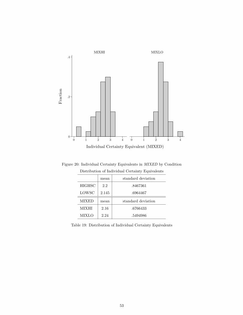
0
.2
.4
0 1 2 3 4 0 1 2 3 4
MIXHI MIXLO
Fra
ctio
n
Individual Certainty Equivalent (MIXED)
Figure 20: Individual Certainty Equivalents in MIXED by Condition
Distribution of Individual Certainty Equivalents
mean standard deviation
HIGHSC 2.2 .8467361
LOWSC 2.145 .6964467
MIXED mean standard deviation
MIXHI 2.16 .6766433
MIXLO 2.24 .5494986
Table 19: Distribution of Individual Certainty Equivalents
53

A.7 Instructions
Welcome to the experiment and thank you for your
participation!
Please do not talk to other participants of the experiment from now on
General information on the procedure
The purpose of this experiment is to investigate economic decision making. You can earn money
during the experiment, which will be paid to you individually and in cash after the experiment has
ended.
The whole experiment takes about 1.5 hours and consists of 3 parts. At the beginning you will
receive detailed instructions for all parts of the experiment. If you have any questions after read-
ing the instructions or at any time during the experiment please raise your hand. One of the
experimenters will then come to you and answer your question in private.
During the experiment, you and the other participants will be asked to make decisions. In some
parts, you will interact with other participants. Thus both your own decisions and the decisions of
other participants can determine your payoffs. Your payoffs are determined according to the rules
which are explained in the following. As long as you can make your decisions, a countdown will be
displayed in the upper right corner of the screen which is intended to give you an orientation for
how much time you should use to make your choices. In most parts you can exceed the time limit if
needed; in some parts, however, you can only act within the time limit (You will be informed about
this beforehand). Information screens not requiring any decisions will disappear after the time-out.
Payment
In some parts of the experiment we will not refer points instead of Euros. Points will be converted to
Euros at the end of the experiment. You will be informed about the exchange rate at the beginning
of the respective part.
For your timely arrival you will receive 4 ¤ additionally to the income earned during the experiment.
Anonymity
We evaluate the data from the experiment only in aggregate and never connect personal information
to data from the experiment. At the end of the experiment you have to sign a receipt, which we
need for our sponsor. The sponsor does not receive any further data from the experiment.
Aid
On your desk you will find a pen. Please leave it on there after the experiment.
54

Part I
Task
The first part of the experiment consists of a task that will last 5 minutes. You will see a black
screen on which words in different colors will appear. Here you can see an example:
You will be asked to click one of the buttons at the bottom of the screen. You will be asked to
choose the button corresponding to the color the word is written in (not the word itself). In the
example you should click on “yellow”.
After clicked a button, the screen disappears and another word in another color appears. Please
try to solve as many word/color combinations as possible within 5 minutes.
After 5 minutes the first part ends automatically and the second part begins.
Payment
You receive 3 ¤ for part I.
Part II
Task
In the second part you first have to answer three questions. For each question answered correctly
you receive 0.5 ¤ = 50 Cents.
Afterwards, you will be shown 10 decision problems. In each of these problems you can choose
between a lottery and a safe amount of money. The lottery remains unchanged within a
55

period, whereas the safe amount of money increases with every additional decision problem. As the
safe amount of money is strictly increasing from row to row, you should stay with the safe amount
of money after you have switched to it once.
Your decision is only valid after you have made a choice for each problem and then confirmed it by
clicking the OK-button on the bottom right of the screen. Take enough time for your decisions, as
your choice – as described in the following – will determine your payoff from this part.
Here you can see what your screen will look like:
Your profit will be determined according to the following rules: First, the computer chooses
randomly and with equal probability one of the ten decision problems for payment. If
you selected the lottery in the relevant problem, the computer will simulate the outcome and you
will receive it as payment. If you selected the safe amount in the relevant problem, you will receive
it for sure.
For example: Assume the computer randomly chooses the first decision problem and you chose the
lottery. Then the computer will simulate the outcomes of this lottery and you either receive 0.2 ¤
(50% probability) or 4.2 ¤ (50% probability).
Payment
56
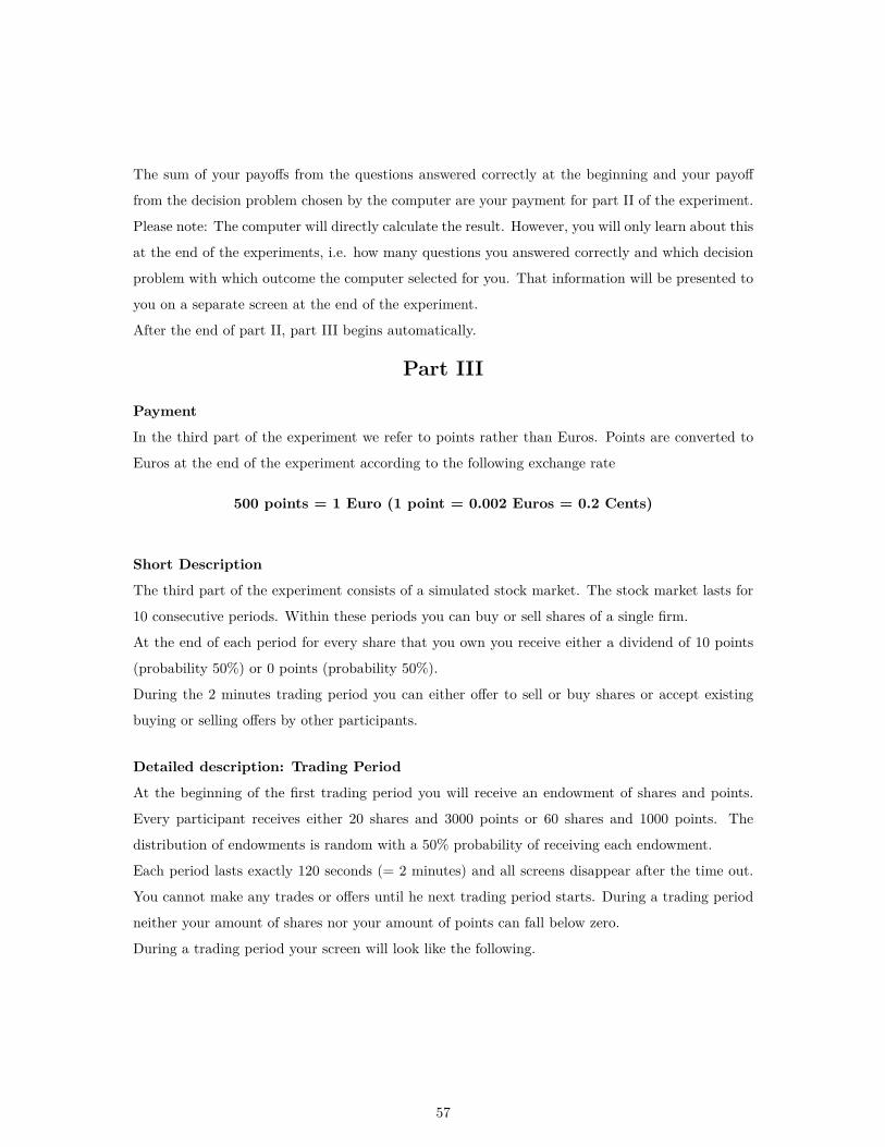
The sum of your payoffs from the questions answered correctly at the beginning and your payoff
from the decision problem chosen by the computer are your payment for part II of the experiment.
Please note: The computer will directly calculate the result. However, you will only learn about this
at the end of the experiments, i.e. how many questions you answered correctly and which decision
problem with which outcome the computer selected for you. That information will be presented to
you on a separate screen at the end of the experiment.
After the end of part II, part III begins automatically.
Part III
Payment
In the third part of the experiment we refer to points rather than Euros. Points are converted to
Euros at the end of the experiment according to the following exchange rate
500 points = 1 Euro (1 point = 0.002 Euros = 0.2 Cents)
Short Description
The third part of the experiment consists of a simulated stock market. The stock market lasts for
10 consecutive periods. Within these periods you can buy or sell shares of a single firm.
At the end of each period for every share that you own you receive either a dividend of 10 points
(probability 50%) or 0 points (probability 50%).
During the 2 minutes trading period you can either offer to sell or buy shares or accept existing
buying or selling offers by other participants.
Detailed description: Trading Period
At the beginning of the first trading period you will receive an endowment of shares and points.
Every participant receives either 20 shares and 3000 points or 60 shares and 1000 points. The
distribution of endowments is random with a 50% probability of receiving each endowment.
Each period lasts exactly 120 seconds (= 2 minutes) and all screens disappear after the time out.
You cannot make any trades or offers until he next trading period starts. During a trading period
neither your amount of shares nor your amount of points can fall below zero.
During a trading period your screen will look like the following.
57

In the upper box you see the current period and how much time you have left in the current
period. Below it to the left the box displays how many shares you currently own and how large
your current wealth is expressed in points. Additionally the current share price and the amount of
available shares and points are displayed.
Available shares are those of your shares that you have not offered for sale yet. If you offer to sell
shares, you still own them, but they will be subtracted from your account as soon as someone else
accepts your offer. Hence, you can only make sale offers that do not exceed your current amount
of available shares.
Available points are those of your points that you have not used for buying offers yet. If you make
an offer to buy shares, you still own the points, but they will be subtracted from your account as
soon as someone else accepts your offer. Hence, you can only make buying offers that do not exceed
your current amount of available points.
On the bottom left you can see a graph that shows the evolution of share prices in the current
period. On the horizontal axis (the x-axis) you can see the time in seconds at which a trade was
made. On the vertical axis (the y-axis) you can see the corresponding price.
In the upper part of the screen you see two lists that have the headlines “Previous Sales” and
“Previous Purchases”. Here, every trade that you made is listed. For each trade where you bought
58

shares, price and quantity will be listed in “Previous Purchases”. For each trade where you sold
shares, price and quantity will be listed in “Previous Sales”.
Below you find two lists with the headlines “Current Selling Offers” and “Current Buying Offers”.
Accepting Selling Offers
In the list “Current Selling Offers” you find price and quantity of each offer, in which a participant
offers to sell shares. Your own selling offers will also appear in this list. You can accept every offer
in this list (except for your own offers) by marking the corresponding entry in the list, entering the
quantity you want to buy into the field “quantity”, and then confirming by clicking on the button
“Buy”. If you accept a selling offer, you will receive the number of shares that you have entered
from the seller and the seller receives the corresponding price for each share he sold to you.
Please note: You can also buy less than the number of shares stated in the offer. In that case the
offer of the seller will remain on display in the list after the trade, but the number of shares on offer
will be reduced by your purchase. Example: A seller makes an offer to sell 10 shares at the price
of 60 points each. A buyer buys 6 of those shares. Then an offer to buy 4 shares at the price of 60
points each will continue to be available to all other participants.
Please note that the computer automatically marks the best selling offer (i.e. the one with the
lowest price) with a blue bar. You can recognize your own offers, as they are not displayed in black
but in blue font.
Accepting offers to buy
In the list “Current Buying Offers” you find price and quantity of each offer, in which a participant
offers to buy shares. Your own buying offers will also appear in this list. You can accept every offer
in this list (except for you own offers) by marking the corresponding entry in the list, entering the
quantity you want to sell into the field “quantity”, and then confirming by clicking on the button
“Sell”. If you accept a buying offer, the other participant will receive the number of shares that you
entered and you receive the corresponding price for each share you sold.
Please note: You can also sell less than the number of shares the buyer offers to buy. In that case
the offer of the buyer will remain on display in the list after the trade, but the number of shares
demanded will be reduced by your sale.
Please note that the computer automatically marks the best buying offer (i.e. the one with the
highest price) with a blue bar. You can recognize your own offers according to their blue font.
Creating Selling or Buying Offers
In the bottom part of the screen you have the possibility to create your own selling or buying offers.
If you want to create an offer to sell, enter the quantity of shares that you want to sell and the price
59
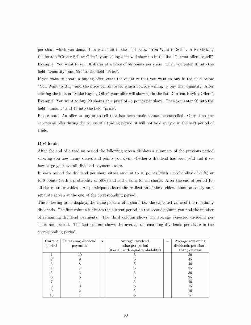
per share which you demand for each unit in the field below “You Want to Sell” . After clicking
the button “Create Selling Offer”, your selling offer will show up in the list “Current offers to sell”.
Example: You want to sell 10 shares at a price of 55 points per share. Then you enter 10 into the
field “Quantity” and 55 into the field “Price”.
If you want to create a buying offer, enter the quantity that you want to buy in the field below
“You Want to Buy” and the price per share for which you are willing to buy that quantity. After
clicking the button “Make Buying Offer” your offer will show up in the list “Current Buying Offers”.
Example: You want to buy 20 shares at a price of 45 points per share. Then you enter 20 into the
field “amount” and 45 into the field “price”.
Please note: An offer to buy or to sell that has been made cannot be cancelled. Only if no one
accepts an offer during the course of a trading period, it will not be displayed in the next period of
trade.
Dividends
After the end of a trading period the following screen displays a summary of the previous period
showing you how many shares and points you own, whether a dividend has been paid and if so,
how large your overall dividend payments were.
In each period the dividend per share either amount to 10 points (with a probability of 50%) or
to 0 points (with a probability of 50%) and is the same for all shares. After the end of period 10,
all shares are worthless. All participants learn the realization of the dividend simultaneously on a
separate screen at the end of the corresponding period.
The following table displays the value pattern of a share, i.e. the expected value of the remaining
dividends. The first column indicates the current period, in the second column you find the number
of remaining dividend payments. The third column shows the average expected dividend per
share and period. The last column shows the average of remaining dividends per share in the
corresponding period.
Current Remaining dividend x Average dividend = Average remainingperiod payments value per period dividends per share
(0 or 10 with equal probability) that you own
1 10 5 502 9 5 453 8 5 404 7 5 355 6 5 306 5 5 257 4 5 208 3 5 159 2 5 1010 1 5 5
60

Assume for example that four trading periods remain. As the dividend per share is either 0 or 10
points with a probability of 50% each, this yields an expected dividend of 5 points per share and
period. Assume you only own one single share which you intend to hold until the market closes.
Then you can expect a total dividend payment for the four remaining periods of ‘4 remaining
periods’ x ‘5 points’ = ‘20 points’.
Payoff
At the end of part III the shares no remaining value. Only your amount of points will be converted
to Euros according to the exchange rate stated above of 1 point = 0.002 Euros = 0.2 Cents.
Afterwards, you will see a screen displaying your payoffs from the second part.
In the following, we will ask you to completely and honestly answer some questions concerning your
person. On leaving the laboratory, we will pay you your profit privately and in cash. Please remain
seated until we call you up in a random order. Please leave the instructions and the pen at your
desk and take your numbered seat card with you.
Practice Period
Before you start today’s experiment with part I, you will first play a practice period of part III
to become familiar with the stock market. The payoff from this practice period will not influence
your final payoff. Please note that the realization of the dividend and your endowment are not
necessarily identical to the first period of part III as the realization is random and endowments will
be randomly assigned.
After completion of the practicing period part I of the experiment begins.
61