Können wir uns die nordeuropäischen Trends der letzten Jahrzehnte erklären?

 Hans von Storch and Armineh BarkhordarianInstitute of Coastal Research, Helmholtz Zentrum Geesthacht, 

Germany

6 November 2014, LASG, SWA, Hamburg

• 

The issue is deconstructing a given record with the intention to identify „predictable“ components.

• First task: Describing change

• Second task: “Detection” - Assessing change if consistent with natural variability (does the explanation need invoking external causes?)

• Third task: “Attribution” – If the presence of a cause is “detected”, determining which mix of causes describes the present change best

Deconstructing change

„Significant“ trends

Often, an anthropogenic influence is assumed to be in operation when trends are found to be „significant“.

• If the null-hypothesis is correctly rejected, then the conclusion to be drawn is – if the data collection exercise would be repeated, then we may expect to see again a similar trend.

• Example: N European warming trend “April to July” as part of the seasonal cycle.

• It does not imply that the trend will continue into the future (beyond the time scale of serial correlation).

• Example: Usually September is cooler than July.

„Significant“ trends

Establishing the statistical significance of a trend may be a necessary condition for claiming that the trend would represent evidence of anthropogenic influence.

Claims of a continuing trend require that the dynamical cause for the present trend is identified, and that the driver causing the trend itself is continuing to operate.

Thus, claims for extension of present trends into the future require- empirical evidence for an ongoing trend, and- theoretical reasoning for driver-response dynamics, and- forecasts of future driver behavior.

5

Anthropogenic

Natural

Internalvariability

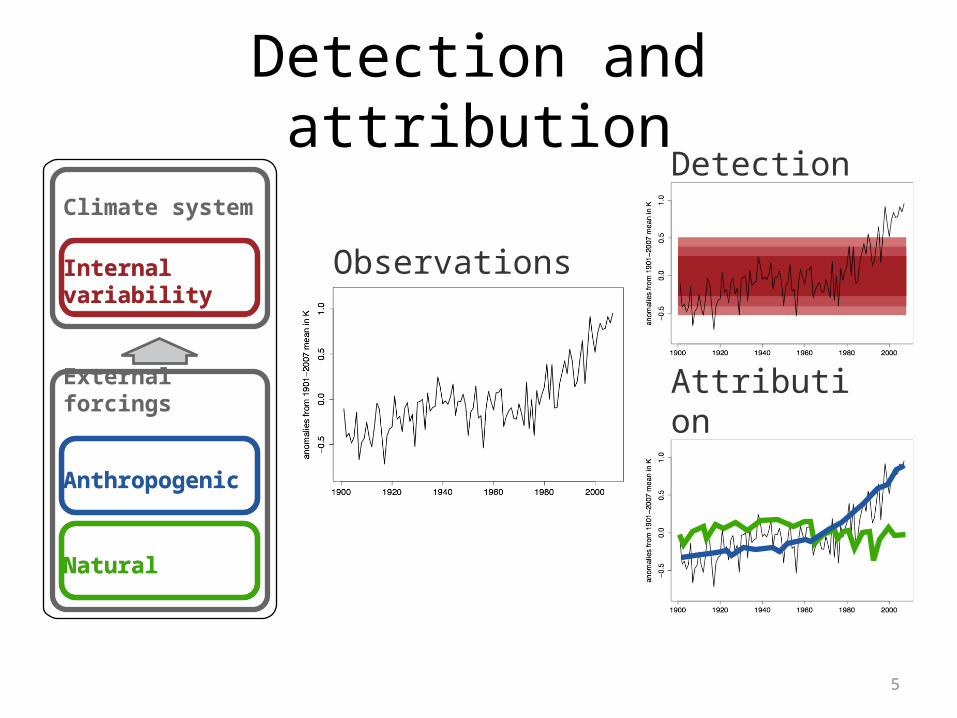
Detection and attribution

Attribution

Anthropogenic

Natural

Observations

External forcings

Climate system

Detection

Internalvariability

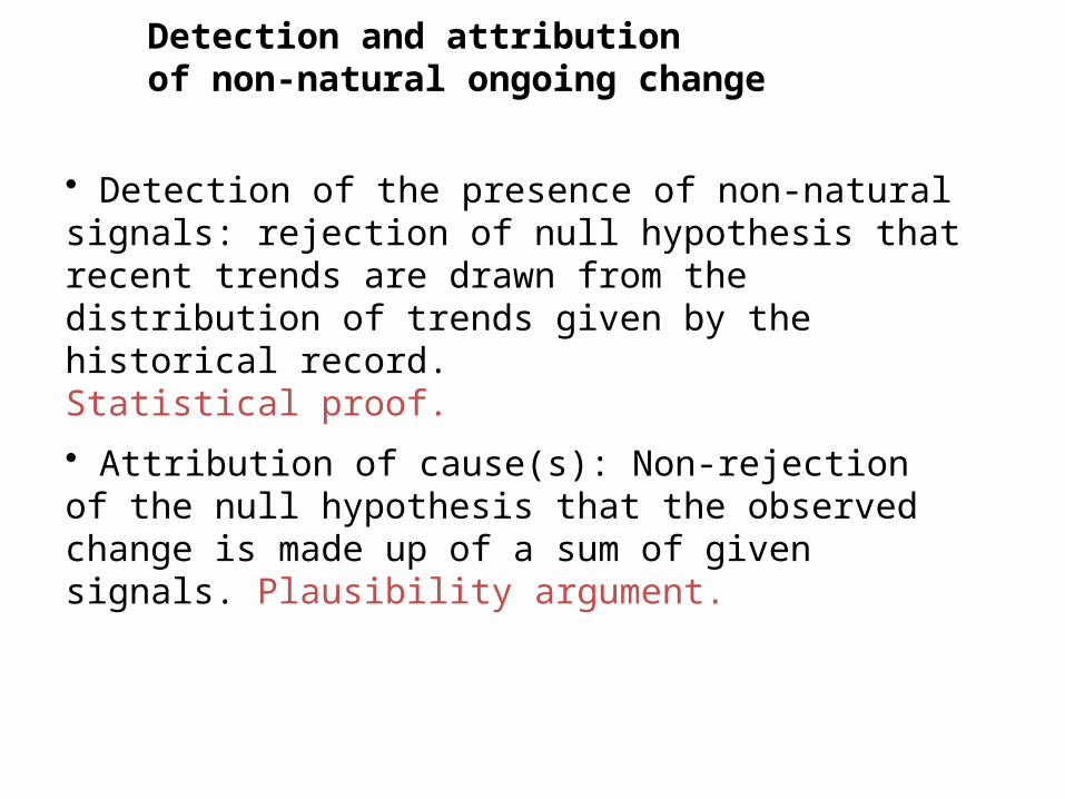
• Detection of the presence of non-natural signals: rejection of null hypothesis that recent trends are drawn from the distribution of trends given by the historical record. Statistical proof.

• Attribution of cause(s): Non-rejection of the null hypothesis that the observed change is made up of a sum of given signals. Plausibility argument.

Detection and attribution of non-natural ongoing change

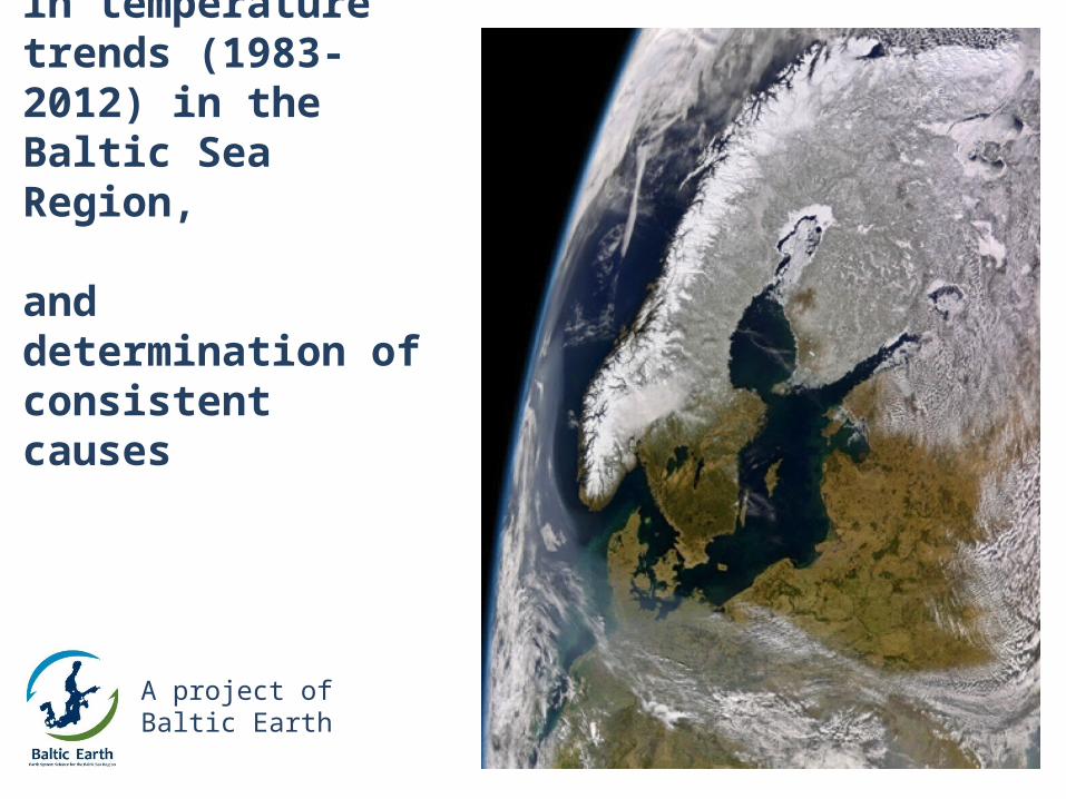
Regional detection of caused changes in temperature trends (1983-2012) in the Baltic Sea Region,

and determination of consistent causes

A project of Baltic Earth

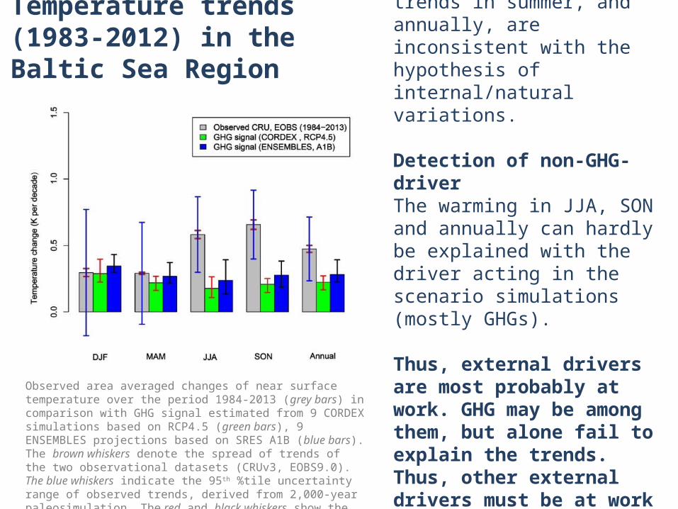
Detection of external driverThe observed (grey) trends in summer, and annually, are inconsistent with the hypothesis of internal/natural variations. 

Detection of non-GHG-driverThe warming in JJA, SON and annually can hardly be explained with the driver acting in the scenario simulations (mostly GHGs). 

Thus, external drivers are most probably at work. GHG may be among them, but alone fail to explain the trends. Thus, other external drivers must be at work as well.

Temperature trends (1983-2012) in the Baltic Sea Region

Observed area averaged changes of near surface temperature over the period 1984-2013 (grey bars) in comparison with GHG signal estimated from 9 CORDEX simulations based on RCP4.5 (green bars), 9 ENSEMBLES projections based on SRES A1B (blue bars). The brown whiskers denote the spread of trends of the two observational datasets (CRUv3, EOBS9.0). The blue whiskers indicate the 95th %tile uncertainty range of observed trends, derived from 2,000-year paleosimulation. The red and black whiskers show the spread of trends of 9 RCP4.5 and 9 A1B climate change projections. 

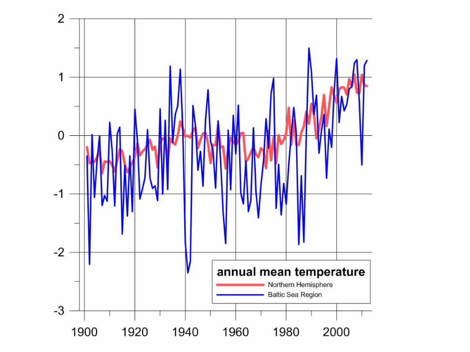
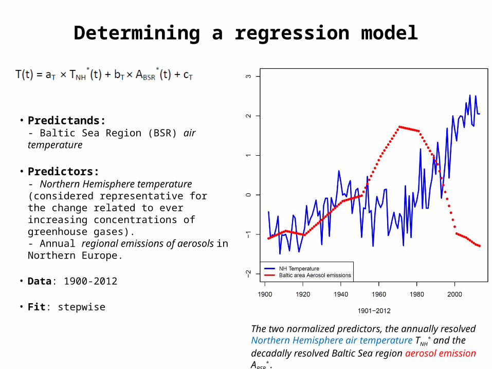
Determining a regression model

The two normalized predictors, the annually resolved Northern Hemisphere air temperature TNH

* and the decadally resolved Baltic Sea region aerosol emission ABSR

* .

• Predictands: - Baltic Sea Region (BSR) air temperature

• Predictors: - Northern Hemisphere temperature (considered representative for the change related to ever increasing concentrations of greenhouse gases).- Annual regional emissions of aerosols in Northern Europe. 

• Data: 1900-2012

• Fit: stepwise

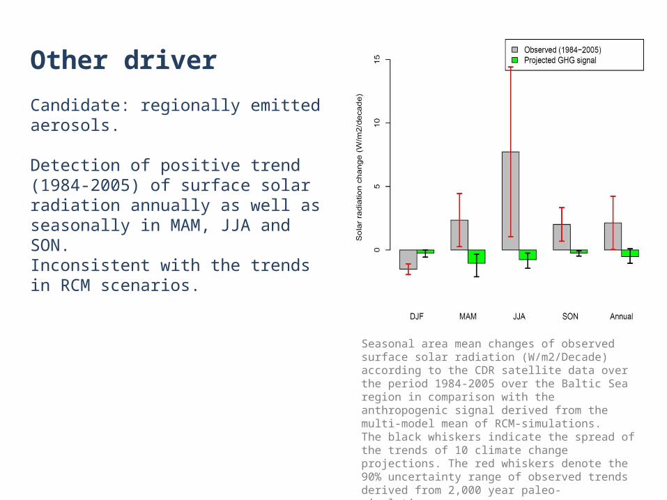
Seasonal area mean changes of observed surface solar radiation (W/m2/Decade) according to the CDR satellite data over the period 1984-2005 over the Baltic Sea region in comparison with the anthropogenic signal derived from the multi-model mean of RCM-simulations. The black whiskers indicate the spread of the trends of 10 climate change projections. The red whiskers denote the 90% uncertainty range of observed trends derived from 2,000 year paleo-simulations.

Other driver

Candidate: regionally emitted aerosols.

Detection of positive trend (1984-2005) of surface solar radiation annually as well as seasonally in MAM, JJA and SON.Inconsistent with the trends in RCM scenarios.

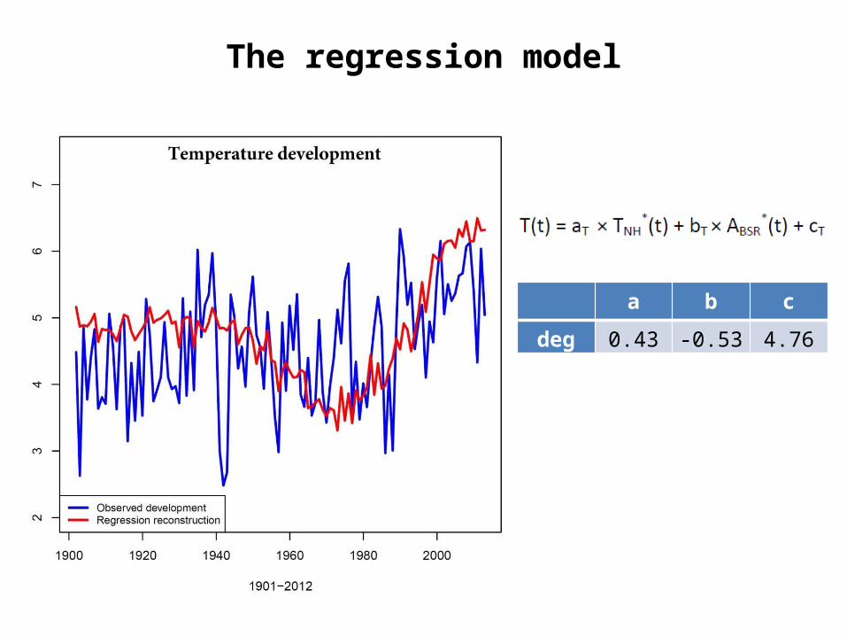
The regression model

a b c

deg 0.43 -0.53 4.76

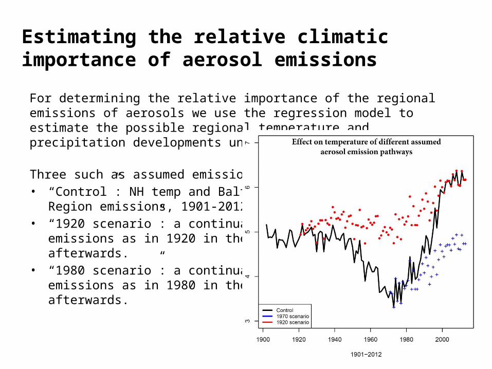
Estimating the relative climatic importance of aerosol emissions

For determining the relative importance of the regional emissions of aerosols we use the regression model to estimate the possible regional temperature and precipitation developments under assumed emissions. 

Three such as assumed emission• “Control”: NH temp and Baltic Sea 

Region emissions, 1901-2012. • “1920 scenario”: a continuation of 

emissions as in 1920 in the years afterwards.

• “1980 scenario”: a continuations of emissions as in 1980 in the years afterwards. 

Conclusions

• The challenge of detection non-natural climate change and attributing it to specific causes, is hardly implemented on regional scales.

• In case of Baltic Sea Region temperature, GHGs are positively insufficient for explaining recent warming patterns

• A plausible co-driver of temperature change is regional aerosol emissions.•  Conditional upon skill of regression model, the relative importance of 

GHG/regional aerosol forcing is about 5/4.• The regression model suggest that the decrease of global temperature before 

1970s and the simultaneous increase in aerosol emissions caused a regional cooling of 1 - 1.5K.

• The strong global temperature increase and the simultaneous decrease of regional aerosols went along with a strong regional temperature increase of 1,5 - 2 K since 1980.

• The inconsistency of RCM scenarios and recent temperature change may originate from the strong regional aerosol influence, which is not considered in the RCM scenarios.

• First results from RCM experimentation point to considerably smaller temp changes. (not shown)

RESULTS NOT STABLE YET

for instance dependent on deatils of fitting regression model (time-focus)