Kolmogorov Superposition Theorem and its application to

wavelet image decompositions

Pierre-Emmanuel Leni, Yohan D. Fougerolle, and Frederic Truchetet

Universite de Bourgogne, Laboratoire LE2I, UMR CNRS 5158,

12 rue de la fonderie, 71200 Le Creusot, France

ABSTRACT

This paper deals with the decomposition of multivariate functions into sums and compositions of monovariatefunctions. The global purpose of this work is to find a suitable strategy to express complex multivariate functionsusing simpler functions that can be analyzed using well know techniques, instead of developing complex N-dimensional tools. More precisely, most of signal processing techniques are applied in 1D or 2D and cannot easilybe extended to higher dimensions. We recall that such a decomposition exists in the Kolmogorov’s superpositiontheorem. According to this theorem, any multivariate function can be decomposed into two types of univariatefunctions, that are called inner and external functions. Inner functions are associated to each dimension andlinearly combined to construct a hash-function that associates every point of a multidimensional space to avalue of the real interval [0, 1]. Every inner function is the argument for one external function. The externalfunctions associate real values in [0, 1] to the image by the multivariate function of the corresponding point ofthe multidimensional space.

Sprecher, in Ref. 1, has proved that internal functions can be used to construct space filling curves, i.e. thereexists a curve that sweeps the multidimensional space and uniquely matches corresponding values into [0, 1]. Ourgoal is to obtain both a new decomposition algorithm for multivariate functions (at least bi-dimensional) andadaptive space filling curves. Two strategies can be applied. Either we construct fixed internal functions to obtainspace filling curves, which allows us to construct an external function such that their sums and compositionsexactly correspond to the multivariate function; or the internal function is constructed by the algorithm and isadapted to the multivariate function, providing different space filling curves for different multivariate functions.

We present two of the most recent constructive algorithms of monovariate functions. The first method isdue to Sprecher (Ref. 2 and Ref. 3). We provide additional explanations to the existing algorithm and presentseveral decomposition results for gray level images. We point out the main drawback of this method: all thefunction parameters are fixed, so the univariate functions cannot be modified; precisely, the inner functioncannot be modified and so the space filling curve. The number of layers depends on the dimension of thedecomposed function. The second algorithm, proposed by Igelnik in Ref. 4, increases the parameters flexibility,but only approximates the monovariate functions: the number of layers is variable, a neural networks optimizesthe monovariate functions and the weights associated to each layer to ensure convergence to the decomposedmultivariate function.

We have implemented both Sprecher’s and Igelnik’s algorithms and present the results of the decompositionsof gray level images. There are artifacts in the reconstructed images, which leads us to apply the algorithm onwavelet decomposition images. We detail the reconstruction quality and the quantity of information containedin Igelnik’s network.

Keywords: Kolmogorov superposition theorem, multidimensional function decomposition, neural network, sig-nal processing, image analysis, wavelets

Further author information:pierre-emmanuel.leni@u-bourgogne.fryohan.fougerolle@u-bourgogne.frfrederic.truchetet@u-bourgogne.fr

1. INTRODUCTION

In 1900, Hilbert has conjectured 23 mathematical problems. Amongst them, the 13rd states that high orderequations cannot be solved by sums and compositions of bivariate functions. 57 years later, Kolmogorov demon-strated his superposition theorem (KST) and proved the existence of monovariate functions, such that everymultivariate functions can be expressed as sums and compositions of monovariate functions. Unfortunately,Kolmogorov did not propose any construction method of these monovariate functions.

The superposition theorem, reformulated and simplified by Sprecher in Ref. 5, can be written as:

Theorem 1.1 (Kolmogorov superposition theorem). Every continuous function defined on the identityhypercube ([0, 1]d noted Id) f : Id −→ R can be written as sums and compositions of continuous monovariatefunctions:

f(x1, ..., xd) =∑2d

n=0 gn

(

ξ(x1 + na, ..., xd + na))

ξ(x1 + na, ..., xd + na) =∑d

i=1 λiψ(xi + an),

(1)

with ψ continuous function, λi and a constants. ψ is called inner function and g(ξ) external function. Theinner function ψ associates every component xi from the real vector (x1, ..., xd) of Id to a value in [0, 1]. Thefunction ξ associates each vector (x1, ..., xd) ∈ Id to a number yn from the interval [0, 1]. These numbers yn arethe arguments of functions gn, that are summed to obtain the function f .

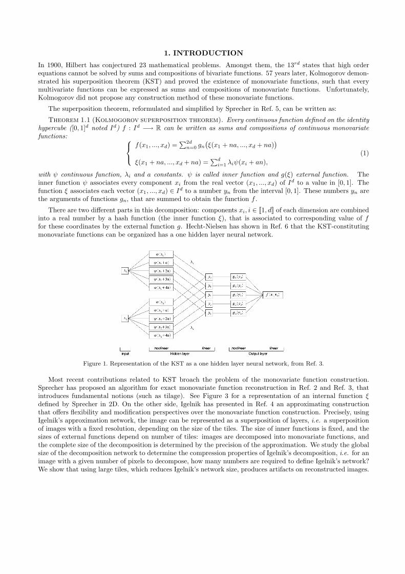
There are two different parts in this decomposition: components xi, i ∈ J1, dK of each dimension are combinedinto a real number by a hash function (the inner function ξ), that is associated to corresponding value of ffor these coordinates by the external function g. Hecht-Nielsen has shown in Ref. 6 that the KST-constitutingmonovariate functions can be organized has a one hidden layer neural network.

Figure 1. Representation of the KST as a one hidden layer neural network, from Ref. 3.

Most recent contributions related to KST broach the problem of the monovariate function construction.Sprecher has proposed an algorithm for exact monovariate function reconstruction in Ref. 2 and Ref. 3, thatintroduces fundamental notions (such as tilage). See Figure 3 for a representation of an internal function ξ

defined by Sprecher in 2D. On the other side, Igelnik has presented in Ref. 4 an approximating constructionthat offers flexibility and modification perspectives over the monovariate function construction. Precisely, usingIgelnik’s approximation network, the image can be represented as a superposition of layers, i.e. a superpositionof images with a fixed resolution, depending on the size of the tiles. The size of inner functions is fixed, and thesizes of external functions depend on number of tiles: images are decomposed into monovariate functions, andthe complete size of the decomposition is determined by the precision of the approximation. We study the globalsize of the decomposition network to determine the compression properties of Igelnik’s decomposition, i.e. for animage with a given number of pixels to decompose, how many numbers are required to define Igelnik’s network?We show that using large tiles, which reduces Igelnik’s network size, produces artifacts on reconstructed images.

We propose to apply Igelnik’s approximation on wavelets image decomposition to reduce the artifacts numberin reconstructed images.

The structure of the paper is as follows: we present Sprecher’s algorithm in section 2, and Igelnik’s algorithmin section 3. In section 4, we present the results of Igelnik’s algorithm applied to the images of a waveletdecomposition. In the last section, we conclude and consider several research perspectives.

Our contributions are a short review of Sprecher’s algorithm and a synthetic explanation of Igelnik’s algorithm.We present the results of the application of both algorithms to gray level images. We point out the lack offlexibility of Sprecher’s algorithm and focus our study on Igelnik’s network. Considering the error reconstructionof this approximation, we apply Igelnik’s network to ”simpler” images: wavelet decomposition images. Wecharacterize the reconstruction quality as a function of tiles density.

2. SPRECHER’S ALGORITHM

We present the algorithm proposed by Sprecher in Ref. 2 and Ref. 3, in which he presents an exact algorithm forinternal and external functions construction, respectively. In Ref. 7, Braun and al. have pointed out that theinternal function ψ defined by Sprecher was discontinuous for several values. They provide a new definition thatensures continuity and monotonicity of the function ψ. The construction of internal functions ψ relies on a realnumber decomposition dk in a given base γ.

Definition 2.1 (Notations).� d is the dimension, d > 2.� m is the number of tilage layers, m > 2d.� γ is the base of the variables xi, γ > m+ 2.� a = 1γ(γ−1) is the translation between two layers of tilage.� λ1 = 1 and for 2 6 i 6 d, λi =

∑

∞

r=11

γ(i−1)(dr−1)/(d−1) are the coefficients of the linear combination, that is

the argument of function g.� every decimal number (noted dk) in [0, 1] with k decimals can be written: dk =∑k

r=1 irγ−r, and dn

k =

dk + n∑k

r=2 γ−r defines a translated dk.

Using the dk defined in definition 2.1, Braun and al. define the function ψ by:

ψk(dk) =

for k = 1 : dk

for k > 1 and ik < γ − 1 : ψk−1(dk − ik

γk ) + ik

γdk

−1d−1

for k > 1 and ik = γ − 1 : 12 (ψk(dk − 1

γk ) + ψk−1(dk + 1γk )).

(2)

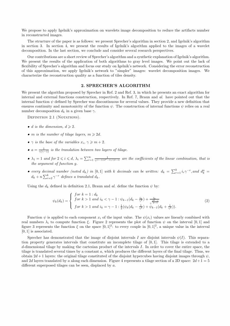
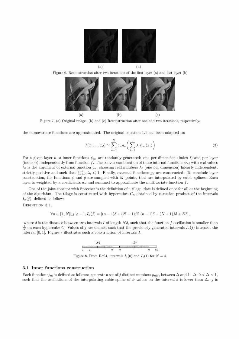
Function ψ is applied to each component xi of the input value. The ψ(xi) values are linearly combined withreal numbers λi to compute function ξ. Figure 2 represents the plot of function ψ on the interval [0, 1] andfigure 3 represents the function ξ on the space [0, 1]2: to every couple in [0, 1]2, a unique value in the interval[0, 1] is associated.

Sprecher has demonstrated that the image of disjoint intervals I are disjoint intervals ψ(I). This separa-tion property generates intervals that constitute an incomplete tilage of [0, 1]. This tilage is extended to ad-dimensional tilage by making the cartesian product of the intervals I. In order to cover the entire space, thetilage is translated several times by a constant a, which produces the different layers of the final tilage. Thus, weobtain 2d+ 1 layers: the original tilage constituted of the disjoint hypercubes having disjoint images through ψ,and 2d layers translated by a along each dimension. Figure 4 represents a tilage section of a 2D space: 2d+1 = 5different superposed tilages can be seen, displaced by a.

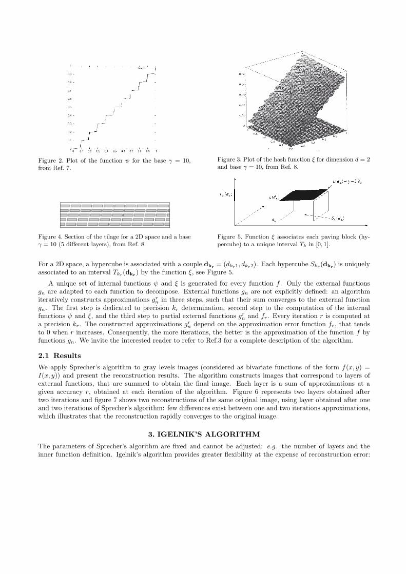
Figure 2. Plot of the function ψ for the base γ = 10,from Ref. 7.

Figure 3. Plot of the hash function ξ for dimension d = 2and base γ = 10, from Ref. 8.

Figure 4. Section of the tilage for a 2D space and a baseγ = 10 (5 different layers), from Ref. 8.

Figure 5. Function ξ associates each paving block (hy-percube) to a unique interval Tk in [0, 1].

For a 2D space, a hypercube is associated with a couple dkr= (dkr1, dkr2). Each hypercube Skr (dkr

) is uniquelyassociated to an interval Tkr(dkr

) by the function ξ, see Figure 5.

A unique set of internal functions ψ and ξ is generated for every function f . Only the external functionsgn are adapted to each function to decompose. External functions gn are not explicitly defined: an algorithmiteratively constructs approximations gr

n in three steps, such that their sum converges to the external functiongn. The first step is dedicated to precision kr determination, second step to the computation of the internalfunctions ψ and ξ, and the third step to partial external functions gr

n and fr. Every iteration r is computed ata precision kr. The constructed approximations gr

n depend on the approximation error function fr, that tendsto 0 when r increases. Consequently, the more iterations, the better is the approximation of the function f byfunctions gn. We invite the interested reader to refer to Ref.3 for a complete description of the algorithm.

2.1 Results

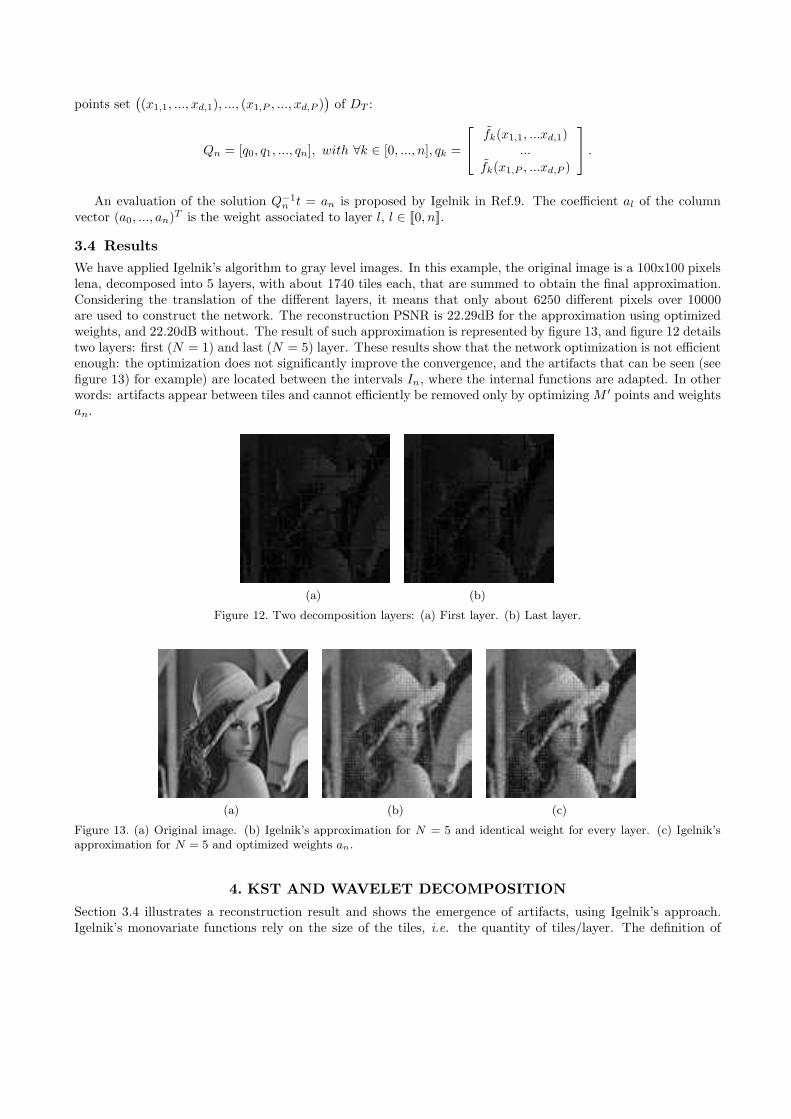
We apply Sprecher’s algorithm to gray levels images (considered as bivariate functions of the form f(x, y) =I(x, y)) and present the reconstruction results. The algorithm constructs images that correspond to layers ofexternal functions, that are summed to obtain the final image. Each layer is a sum of approximations at agiven accuracy r, obtained at each iteration of the algorithm. Figure 6 represents two layers obtained aftertwo iterations and figure 7 shows two reconstructions of the same original image, using layer obtained after oneand two iterations of Sprecher’s algorithm: few differences exist between one and two iterations approximations,which illustrates that the reconstruction rapidly converges to the original image.

3. IGELNIK’S ALGORITHM

The parameters of Sprecher’s algorithm are fixed and cannot be adjusted: e.g. the number of layers and theinner function definition. Igelnik’s algorithm provides greater flexibility at the expense of reconstruction error:

(a) (b)

Figure 6. Reconstruction after two iterations of the first layer (a) and last layer (b)

(a) (b) (c)

Figure 7. (a) Original image. (b) and (c) Reconstruction after one and two iterations, respectively.

the monovariate functions are approximated. The original equation 1.1 has been adapted to:

f(x1, ..., xd) ≃

N∑

n=1

angn

( d∑

i=1

λiψni(xi)

)

(3)

For a given layer n, d inner functions ψni are randomly generated: one per dimension (index i) and per layer(index n), independently from function f . The convex combination of these internal functions ψni with real valuesλi is the argument of external function gn, choosing real numbers λi (one per dimension) linearly independent,

strictly positive and such that∑d

i=1 λi 6 1. Finally, external functions gn are constructed. To conclude layerconstruction, the functions ψ and g are sampled with M points, that are interpolated by cubic splines. Eachlayer is weighted by a coefficients an and summed to approximate the multivariate function f .

One of the joint concept with Sprecher is the definition of a tilage, that is defined once for all at the beginningof the algorithm. The tilage is constituted with hypercubes Cn obtained by cartesian product of the intervalsIn(j), defined as follows:

Definition 3.1.

∀n ∈ J1, NK, j > −1, In(j) = [(n− 1)δ + (N + 1)jδ, (n− 1)δ + (N + 1)jδ +Nδ],

where δ is the distance between two intervals I of length Nδ, such that the function f oscillation is smaller than1N

on each hypercube C. Values of j are defined such that the previously generated intervals In(j) intersect theinterval [0, 1]. Figure 8 illustrates such a construction of intervals I.

Figure 8. From Ref.4, intervals I1(0) and I1(1) for N = 4.

3.1 Inner functions construction

Each function ψni is defined as follows: generate a set of j distinct numbers ynij , between ∆ and 1−∆, 0 < ∆ < 1,such that the oscillations of the interpolating cubic spline of ψ values on the interval δ is lower than ∆. j is

given by definition 3.1. The real numbers ynij are sorted, i.e.: ynij < ynij+1. The image of the interval In(j)by function ψ is ynij . This discontinuous inner function ψ is sampled by M points, that are interpolated by acubic spline. We obtain two sets of points: points located on plateaus over intervals In(j), and points M ′ locatedbetween two intervals In(j) and In(j+1), that are randomly placed. Points M ′ are optimized during the neuralnetwork construction, using a stochastic approach. Figure 9(a) represents final function ψ on the interval [0, 1],and figure 9(b) illustrates a construction example of function ψ for two consecutive intervals In(j) and In(j+1).

Once functions ψni are constructed, the function ξn(x) =∑d

i=1 λiψni(x) can be evaluated. On hypercubes

Cnij1,...,jd, the function ξ has constant values pnj1,...,jd

=∑d

i=1 λiyniji . Every random number yniji generatedverifies that the generated values pniji are all different, ∀i ∈ J1, dK, ∀n ∈ J1, NK, ∀j ∈ N, j > −1.

(a) (b)

Figure 9. (a) Example of function ψ sampled by 500 points that are interpolated by a cubic spline. (b) From Ref.4, plotof ψ. On the intervals In(j) and In(j + 1), ψ has constant values, respectively ynij and ynij+1.

3.2 External function construction

The function gn is defined as follows:� For every real number t = pn,j1,...,jd, function gn(t) is equal to the N th of values of the function f at the

center of the hypercube Cnij1,...,jd, noted bn,j1,...,jd

, i.e.: gn(pn,j1,...,jd) = 1

Nbn,j1,...,jd

.� The definition interval of function gn is extended to all t ∈ [0, 1]. Consider A(tA, gn(tA)) and D(tD, gn(tD))two adjacent points, where tA and tD are two levels pn,j1,...,jd

. Two points B et C are placed in A and D

neighborhood, respectively. PointsB and C are connected with a line defined with a slope r = gn(tC)−gn(tB)tC−tB

.PointsA(tA, gn(tA)) andB(tB , gn(tB)) are connected with a nine degree spline s, such that: s(tA) = gn(tA),s(tB) = gn(tB), s′(tB) = r, and s(2)(tB) = s(3)(tB) = s(4)(tB) = 0. Points C and D are connected with asimilar nine degree spline. The connection condition at points A and D of both nine degree splines givesthe remaining conditions. Figure 10(a) illustrates this construction, whereas (b) gives a complete overviewof the function gn for a layer.

Remark 1. Points A and D (values of function f at the centers of the hypercubes) are not regularly spaced onthe interval [0, 1], since their abscissas are given by function ξ, and depend on random values ynij ∈ [0, 1]. Theplacement of points B and C in the circles centered in A and D must preserve the order of points: A,B,C,D,i.e. the radius of these circles must be smaller than half of the length between the two points A and D.

The external function has a noisy shape, which is related to the global sweeping scheme of the image: Sprecherand al. have demonstrated in Ref.1 that using internal functions, space-filling curves can be defined. Functionξ associates a unique real value to every couple (dkr1, dkr2) of the multidimensional space [0, 1]d. Sorting thesereal values defines a unique path through the tiles of a layer: the space filling curve. Figure 11 illustrates anexample of such a curve: the pixels are swept without any neighborhood property conservation.

(a) (b)

Figure 10. (a) From Ref.4, plot of gn. Points A and D are obtained with function ξ and function f . (b) Example offunction gn for a complete layer of lena decomposition.

Figure 11. Igelnik’s space filling curve.

3.3 Neural network stochastic construction

Igelnik defines parameters during construction that are optimized using a stochastic method (ensemble approach):the weights an associated to each layer, and the placement of the sampling points M ′ of inner functions ψ thatare located between two consecutive intervals.To evaluate the network convergence, three sets of points are constituted: a training set DT , a generalization setDG, and a validation set DV .N layers are successively built. To add a new layer, K candidate layers are generated with the same plateausynij , which gives K new candidate neural networks. The difference between two candidate layers is the set ofsampling points located between two intervals In(j) and In(j+ 1), that are randomly chosen. We keep the layerfrom the network with the smallest mean squared error that is evaluated using the generalization set DG. Theweights an are obtained by minimizing the difference between the approximation given by the neural networkand the image of function f for the points of the training set DT . The algorithm is iterated until N layers areconstructed. The validation error of the final neural network is determined using validation set DV .

To determine coefficients an, the difference between f and its approximation f must be minimized:

‖Qnan − t‖ , noting t =

f(x1,1, ..., xd,1)...

f(x1,P , ..., xd,P )

, (4)

with Qn a matrix of column vectors qk, k ∈ J0, nK that corresponds to the approximation (f) of the kth layer for

points set(

(x1,1, ..., xd,1), ..., (x1,P , ..., xd,P ))

of DT :

Qn = [q0, q1, ..., qn], with ∀k ∈ [0, ..., n], qk =

fk(x1,1, ...xd,1)...

fk(x1,P , ...xd,P )

.

An evaluation of the solution Q−1n t = an is proposed by Igelnik in Ref.9. The coefficient al of the column

vector (a0, ..., an)T is the weight associated to layer l, l ∈ J0, nK.

3.4 Results

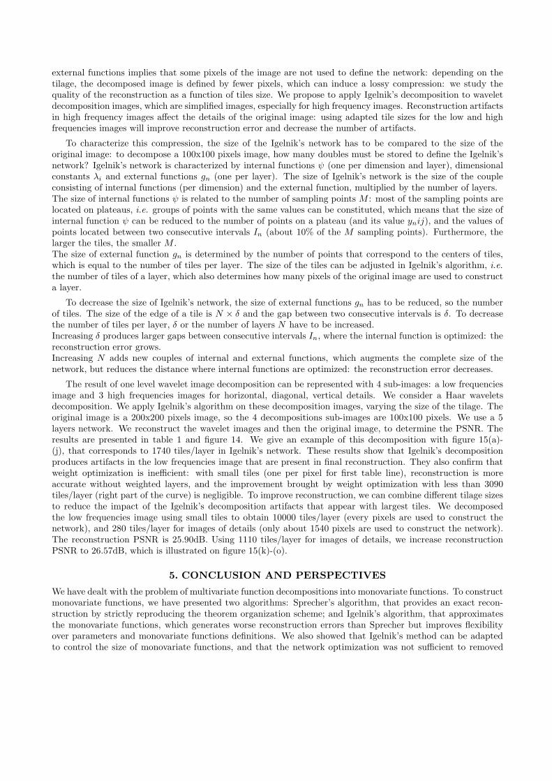
We have applied Igelnik’s algorithm to gray level images. In this example, the original image is a 100x100 pixelslena, decomposed into 5 layers, with about 1740 tiles each, that are summed to obtain the final approximation.Considering the translation of the different layers, it means that only about 6250 different pixels over 10000are used to construct the network. The reconstruction PSNR is 22.29dB for the approximation using optimizedweights, and 22.20dB without. The result of such approximation is represented by figure 13, and figure 12 detailstwo layers: first (N = 1) and last (N = 5) layer. These results show that the network optimization is not efficientenough: the optimization does not significantly improve the convergence, and the artifacts that can be seen (seefigure 13) for example) are located between the intervals In, where the internal functions are adapted. In otherwords: artifacts appear between tiles and cannot efficiently be removed only by optimizing M ′ points and weightsan.

(a) (b)

Figure 12. Two decomposition layers: (a) First layer. (b) Last layer.

(a) (b) (c)

Figure 13. (a) Original image. (b) Igelnik’s approximation for N = 5 and identical weight for every layer. (c) Igelnik’sapproximation for N = 5 and optimized weights an.

4. KST AND WAVELET DECOMPOSITION

Section 3.4 illustrates a reconstruction result and shows the emergence of artifacts, using Igelnik’s approach.Igelnik’s monovariate functions rely on the size of the tiles, i.e. the quantity of tiles/layer. The definition of

external functions implies that some pixels of the image are not used to define the network: depending on thetilage, the decomposed image is defined by fewer pixels, which can induce a lossy compression: we study thequality of the reconstruction as a function of tiles size. We propose to apply Igelnik’s decomposition to waveletdecomposition images, which are simplified images, especially for high frequency images. Reconstruction artifactsin high frequency images affect the details of the original image: using adapted tile sizes for the low and highfrequencies images will improve reconstruction error and decrease the number of artifacts.

To characterize this compression, the size of the Igelnik’s network has to be compared to the size of theoriginal image: to decompose a 100x100 pixels image, how many doubles must be stored to define the Igelnik’snetwork? Igelnik’s network is characterized by internal functions ψ (one per dimension and layer), dimensionalconstants λi and external functions gn (one per layer). The size of Igelnik’s network is the size of the coupleconsisting of internal functions (per dimension) and the external function, multiplied by the number of layers.The size of internal functions ψ is related to the number of sampling points M : most of the sampling points arelocated on plateaus, i.e. groups of points with the same values can be constituted, which means that the size ofinternal function ψ can be reduced to the number of points on a plateau (and its value ynij), and the values ofpoints located between two consecutive intervals In (about 10% of the M sampling points). Furthermore, thelarger the tiles, the smaller M .The size of external function gn is determined by the number of points that correspond to the centers of tiles,which is equal to the number of tiles per layer. The size of the tiles can be adjusted in Igelnik’s algorithm, i.e.the number of tiles of a layer, which also determines how many pixels of the original image are used to constructa layer.

To decrease the size of Igelnik’s network, the size of external functions gn has to be reduced, so the numberof tiles. The size of the edge of a tile is N × δ and the gap between two consecutive intervals is δ. To decreasethe number of tiles per layer, δ or the number of layers N have to be increased.Increasing δ produces larger gaps between consecutive intervals In, where the internal function is optimized: thereconstruction error grows.Increasing N adds new couples of internal and external functions, which augments the complete size of thenetwork, but reduces the distance where internal functions are optimized: the reconstruction error decreases.

The result of one level wavelet image decomposition can be represented with 4 sub-images: a low frequenciesimage and 3 high frequencies images for horizontal, diagonal, vertical details. We consider a Haar waveletsdecomposition. We apply Igelnik’s algorithm on these decomposition images, varying the size of the tilage. Theoriginal image is a 200x200 pixels image, so the 4 decompositions sub-images are 100x100 pixels. We use a 5layers network. We reconstruct the wavelet images and then the original image, to determine the PSNR. Theresults are presented in table 1 and figure 14. We give an example of this decomposition with figure 15(a)-(j), that corresponds to 1740 tiles/layer in Igelnik’s network. These results show that Igelnik’s decompositionproduces artifacts in the low frequencies image that are present in final reconstruction. They also confirm thatweight optimization is inefficient: with small tiles (one per pixel for first table line), reconstruction is moreaccurate without weighted layers, and the improvement brought by weight optimization with less than 3090tiles/layer (right part of the curve) is negligible. To improve reconstruction, we can combine different tilage sizesto reduce the impact of the Igelnik’s decomposition artifacts that appear with largest tiles. We decomposedthe low frequencies image using small tiles to obtain 10000 tiles/layer (every pixels are used to construct thenetwork), and 280 tiles/layer for images of details (only about 1540 pixels are used to construct the network).The reconstruction PSNR is 25.90dB. Using 1110 tiles/layer for images of details, we increase reconstructionPSNR to 26.57dB, which is illustrated on figure 15(k)-(o).

5. CONCLUSION AND PERSPECTIVES

We have dealt with the problem of multivariate function decompositions into monovariate functions. To constructmonovariate functions, we have presented two algorithms: Sprecher’s algorithm, that provides an exact recon-struction by strictly reproducing the theorem organization scheme; and Igelnik’s algorithm, that approximatesthe monovariate functions, which generates worse reconstruction errors than Sprecher but improves flexibilityover parameters and monovariate functions definitions. We also showed that Igelnik’s method can be adaptedto control the size of monovariate functions, and that the network optimization was not sufficient to removed

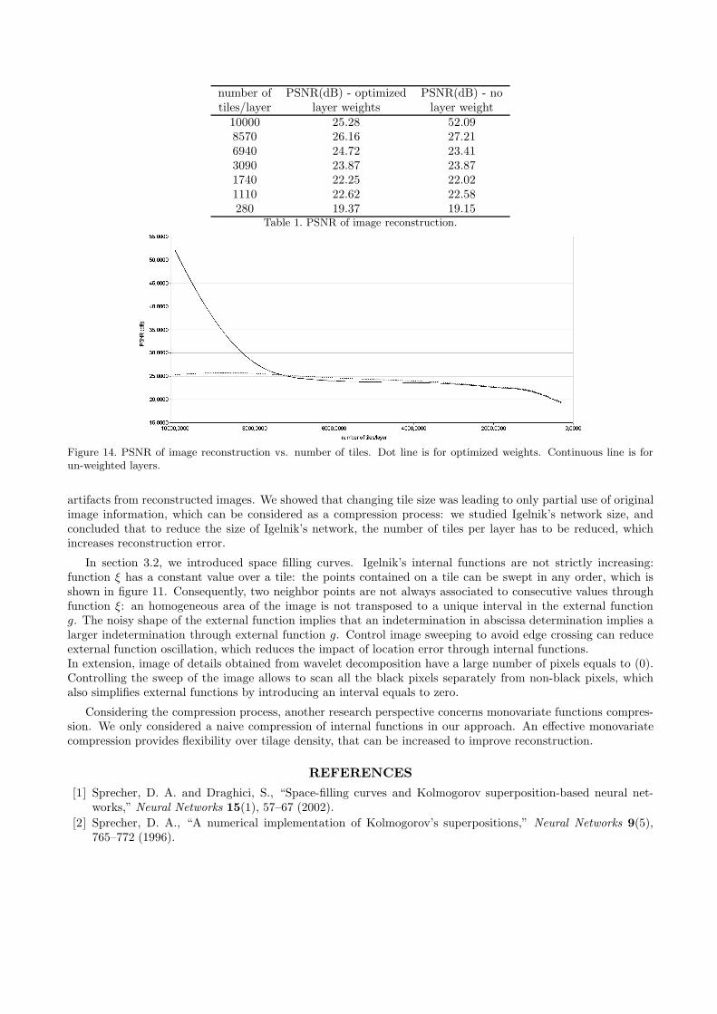
number of PSNR(dB) - optimized PSNR(dB) - notiles/layer layer weights layer weight

10000 25.28 52.098570 26.16 27.216940 24.72 23.413090 23.87 23.871740 22.25 22.021110 22.62 22.58280 19.37 19.15

Table 1. PSNR of image reconstruction.

Figure 14. PSNR of image reconstruction vs. number of tiles. Dot line is for optimized weights. Continuous line is forun-weighted layers.

artifacts from reconstructed images. We showed that changing tile size was leading to only partial use of originalimage information, which can be considered as a compression process: we studied Igelnik’s network size, andconcluded that to reduce the size of Igelnik’s network, the number of tiles per layer has to be reduced, whichincreases reconstruction error.

In section 3.2, we introduced space filling curves. Igelnik’s internal functions are not strictly increasing:function ξ has a constant value over a tile: the points contained on a tile can be swept in any order, which isshown in figure 11. Consequently, two neighbor points are not always associated to consecutive values throughfunction ξ: an homogeneous area of the image is not transposed to a unique interval in the external functiong. The noisy shape of the external function implies that an indetermination in abscissa determination implies alarger indetermination through external function g. Control image sweeping to avoid edge crossing can reduceexternal function oscillation, which reduces the impact of location error through internal functions.In extension, image of details obtained from wavelet decomposition have a large number of pixels equals to (0).Controlling the sweep of the image allows to scan all the black pixels separately from non-black pixels, whichalso simplifies external functions by introducing an interval equals to zero.

Considering the compression process, another research perspective concerns monovariate functions compres-sion. We only considered a naive compression of internal functions in our approach. An effective monovariatecompression provides flexibility over tilage density, that can be increased to improve reconstruction.

REFERENCES

[1] Sprecher, D. A. and Draghici, S., “Space-filling curves and Kolmogorov superposition-based neural net-works,” Neural Networks 15(1), 57–67 (2002).

[2] Sprecher, D. A., “A numerical implementation of Kolmogorov’s superpositions,” Neural Networks 9(5),765–772 (1996).

(a) (b) (c) (d) (e)

(f) (g) (h) (i) (j)

(k) (l) (m) (n) (o)

Figure 15. (a)(b)(c)(d) Wavelet decomposition of lena (low frequencies image, horizontal, diagonal and vertical imageof details, respectively). (e) Direct reconstruction using (a)(b)(c)(d). (f)(g)(h)(i) Corresponding reconstructions usingIgelnik’s network with 1740 tiles/layer, and (j) the final reconstruction. (k)(l)(m)(n) Reconstruction of (a)(b)(c)(d) withdifferent tilage densities, and (o) the final reconstruction.

[3] Sprecher, D. A., “A numerical implementation of Kolmogorov’s superpositions ii,” Neural Networks 10(3),447–457 (1997).

[4] Igelnik, B. and Parikh, N., “Kolmogorov’s spline network,” IEEE transactions on neural networks 14(4),725–733 (2003).

[5] Sprecher, D. A., “An improvement in the superposition theorem of Kolmogorov,” Journal of MathematicalAnalysis and Applications 38, 208–213 (1972).

[6] Hecht-Nielsen, R., “Kolmogorov’s mapping neural network existence theorem,” Proceedings of the IEEEInternational Conference on Neural Networks III, New York , 11–13 (1987).

[7] Braun, J. and Griebel, M., “On a constructive proof of Kolmogorov’s superposition theorem,” Constructiveapproximation (2007).

[8] Brattka, V., “Du 13-ieme probleme de Hilbert a la theorie des reseaux de neurones : aspects constructifs dutheoreme de superposition de Kolmogorov,” L’heritage de Kolmogorov en mathematiques. Editions Belin,Paris. , 241–268 (2004).

[9] Igelnik, B., Pao, Y.-H., LeClair, S. R., and Shen, C. Y., “The ensemble approach to neural-network learningand generalization,” IEEE Transactions on Neural Networks 10, 19–30 (1999).

[10] Igelnik, B., Tabib-Azar, M., and LeClair, S. R., “A net with complex weights,” IEEE Transactions onNeural Networks 12, 236–249 (2001).

[11] Koppen, M., “On the training of a Kolmogorov Network,” Lecture Notes in Computer Science, SpringerBerlin 2415, 140 (2002).

[12] Lagunas, M. A., Perez-Neira, A., Najar, M., and Pages, A., “The Kolmogorov Signal Processor,” LectureNotes in Computer Science, Springer Berlin 686, 494–512 (1993).

[13] Moon, B., “An explicit solution for the cubic spline interpolation for functions of a single variable,” AppliedMathematics and Computation 117, 251–255 (2001).