Embed Size (px)
Citation preview
© ABB Group 09 May, 2014 | Slide 1
Applications of Computational Mathematics to Industrial Products and ProcessesThe Case of ABB
L. Ghezzi, A. Sciacca, F. Rigamonti / ABB Italy – Mathematics for the Digital Factory, Berlin May 2014
Contents
ABB company overview
Applications to products
Applications to processes
Future research trends
© ABB Group 09 May, 2014 | Slide 2
© ABBMay, 2014 | Slide 3
ABB Company Overview
© ABB Group
| Slide 4
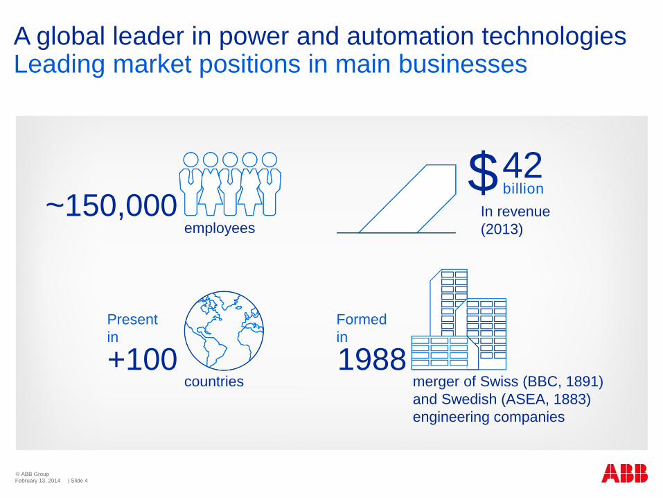
A global leader in power and automation technologiesLeading market positions in main businesses
February 13, 2014
~150,000employees
Present
in
countries+100
Formed
in
1988merger of Swiss (BBC, 1891)
and Swedish (ASEA, 1883)
engineering companies
In revenue
(2013)
billion42$

© ABB Group
| Slide 5
Power and productivity for a better worldABB’s vision
February 13, 2014
As one of the world’s leading engineering companies, we
help our customers to use electrical power efficiently, to
increase industrial productivity and to lower environmental
impact in a sustainable way.

© ABB Group
| Slide 6
Power and automation are all around usYou will find ABB technology…
February 13, 2014
crossing oceans and on the sea bed,
orbiting the earth and working beneath it,
on the trains we ride and in the facilities
that process our water,
in the fields that grow our crops and
packing the food we eat,
in the plants that generate our power and
in our homes, offices and factories
© ABB Group
| Slide 7
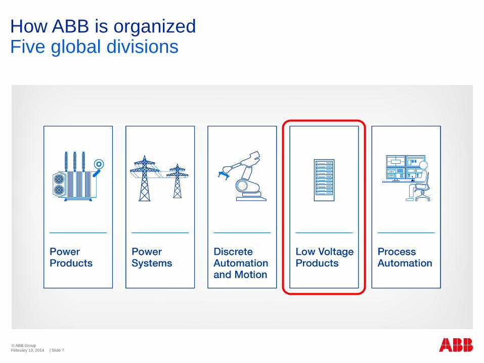
How ABB is organizedFive global divisions
February 13, 2014
© ABB Group
Low Voltage Products division
09 May, 2014 | Slide 8
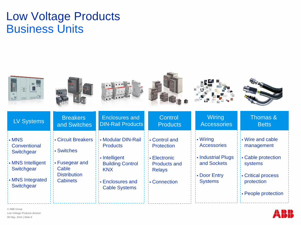
Low Voltage ProductsBusiness Units
MNS
Conventional
Switchgear
MNS Intelligent
Switchgear
MNS Integrated
Switchgear
Circuit Breakers
Switches
Fusegear and
Cable
Distribution
Cabinets
Modular DIN-Rail
Products
Intelligent
Building Control
KNX
Enclosures and
Cable Systems
Control and
Protection
Electronic
Products and
Relays
Connection
Wiring
Accessories
Industrial Plugs
and Sockets
Door Entry
Systems
Breakers
and SwitchesLV Systems
Enclosures and
DIN-Rail Products
Control
Products
Wiring
Accessories
Wire and cable
management
Cable protection
systems
Critical process
protection
People protection
Thomas &
Betts
© ABB Group
Low Voltage Products division
09 May, 2014 | Slide 9
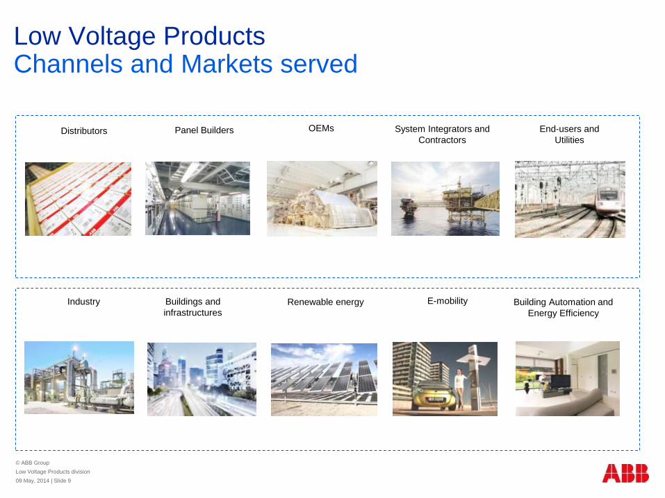
Low Voltage ProductsChannels and Markets served
Distributors Panel Builders OEMs End-users and
Utilities
Industry Buildings and
infrastructuresRenewable energy E-mobility
System Integrators and
Contractors
Building Automation and
Energy Efficiency

© ABBMay, 2014 | Slide 10
Applications to Products
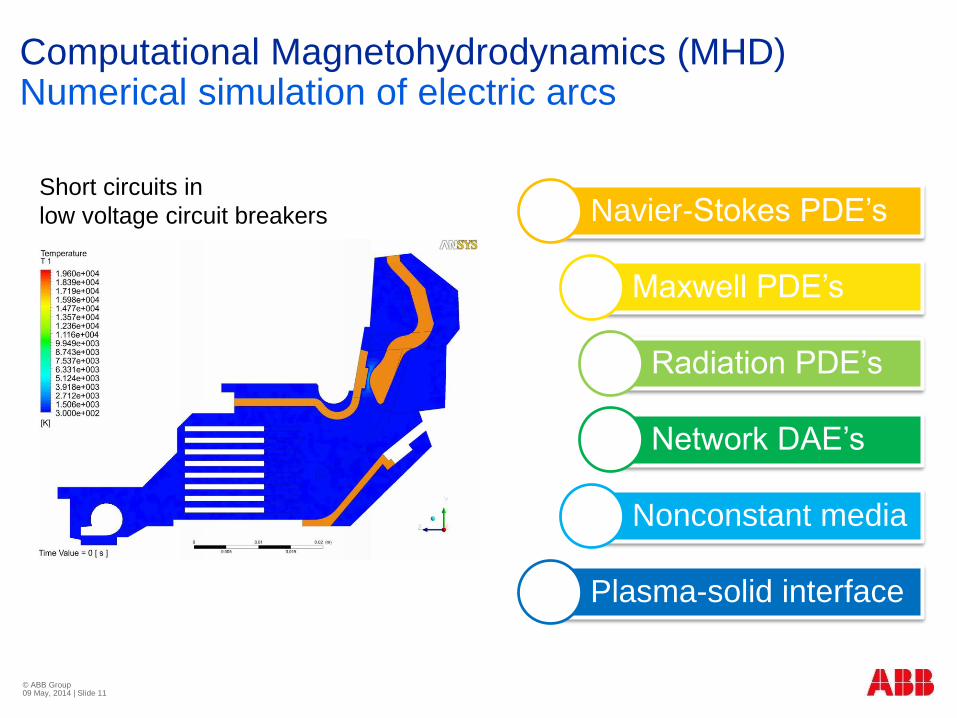
Computational Magnetohydrodynamics (MHD)Numerical simulation of electric arcs
© ABB Group 09 May, 2014 | Slide 11
Navier-Stokes PDE’s
Maxwell PDE’s
Radiation PDE’s
Network DAE’s
Nonconstant media
Plasma-solid interface
Short circuits in
low voltage circuit breakers
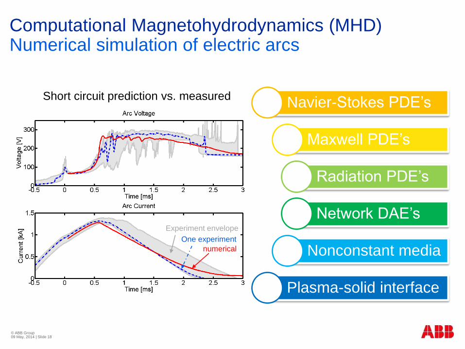
numerical
One experiment
Experiment envelope
Short circuit prediction vs. measured
Computational Magnetohydrodynamics (MHD)Numerical simulation of electric arcs
© ABB Group 09 May, 2014 | Slide 18
Navier-Stokes PDE’s
Maxwell PDE’s
Radiation PDE’s
Network DAE’s
Nonconstant media
Plasma-solid interface

© ABBMay, 2014 | Slide 19
Applications to Processes

Stock sizingOverview
© ABB Group 09 May, 2014 | Slide 20
Time
Stock
level
Safety
stock
(re-order
point)
Re-order
issued
Supply
lead time
𝐿
𝐷
1
Demand
(average)
Re-order
lot
supplied
Re-o
rde
r lo
t
𝑆 = 𝐷𝐿 + 𝑟𝑄
𝑆
Deterministic model
Ordered quantity
(average)𝑄𝑟𝑄
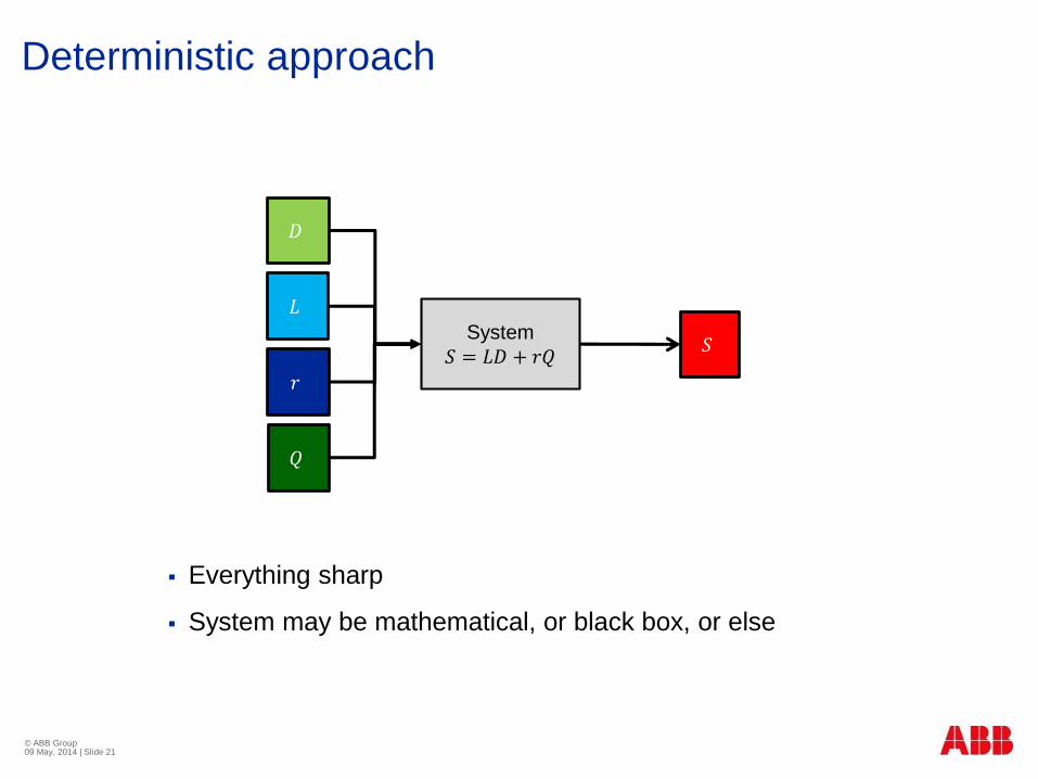
Deterministic approach
Everything sharp
System may be mathematical, or black box, or else
© ABB Group 09 May, 2014 | Slide 21
System
𝑆 = 𝐿𝐷 + 𝑟𝑄
𝑟
𝑆
𝐷
𝐿
𝑄

Stock sizingStochastic problem
© ABB Group 09 May, 2014 | Slide 23
Time
Stock
level
𝐿
𝑆 = 𝐷𝐿 + 𝑟𝑄
𝑆
𝐷 as a Stochastic variable
𝑄𝑟𝑄
𝐷
1
Stock-out!
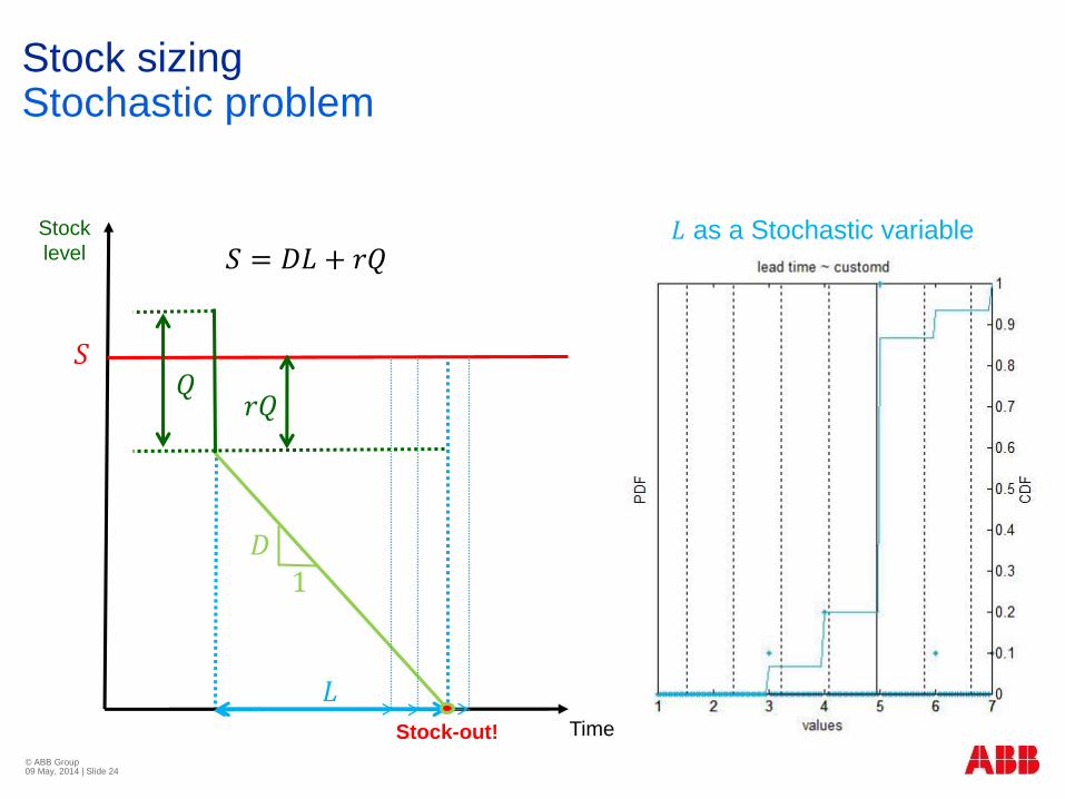
Stock sizingStochastic problem
© ABB Group 09 May, 2014 | Slide 24
Time
Stock
level
𝐿
𝑆 = 𝐷𝐿 + 𝑟𝑄
𝑆
𝐿 as a Stochastic variable
𝑄𝑟𝑄
𝐷
1
Stock-out!

Stock sizingStochastic problem
© ABB Group 09 May, 2014 | Slide 25
Time
Stock
level
𝐿
𝑆 = 𝐷𝐿 + 𝑟𝑄
𝑆
𝑟 as a Stochastic variable
𝑄𝑟𝑄
𝐷
1
Stock-out!
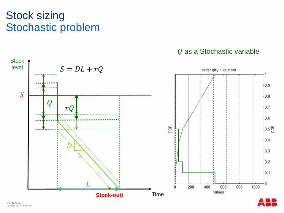
Stock sizingStochastic problem
© ABB Group 09 May, 2014 | Slide 26
Time
Stock
level
𝐿
𝑆 = 𝐷𝐿 + 𝑟𝑄
𝑆
𝑄 as a Stochastic variable
𝑄𝑟𝑄
𝐷
1
Stock-out!
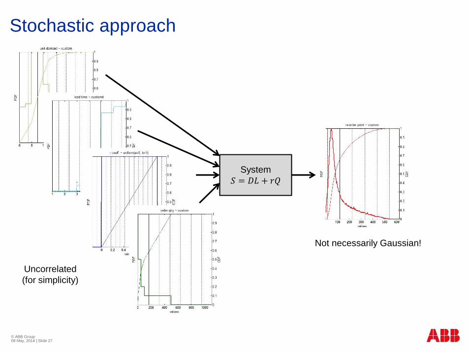
Stochastic approach
© ABB Group 09 May, 2014 | Slide 27
System
𝑆 = 𝐷𝐿 + 𝑟𝑄
Not necessarily Gaussian!
Uncorrelated
(for simplicity)
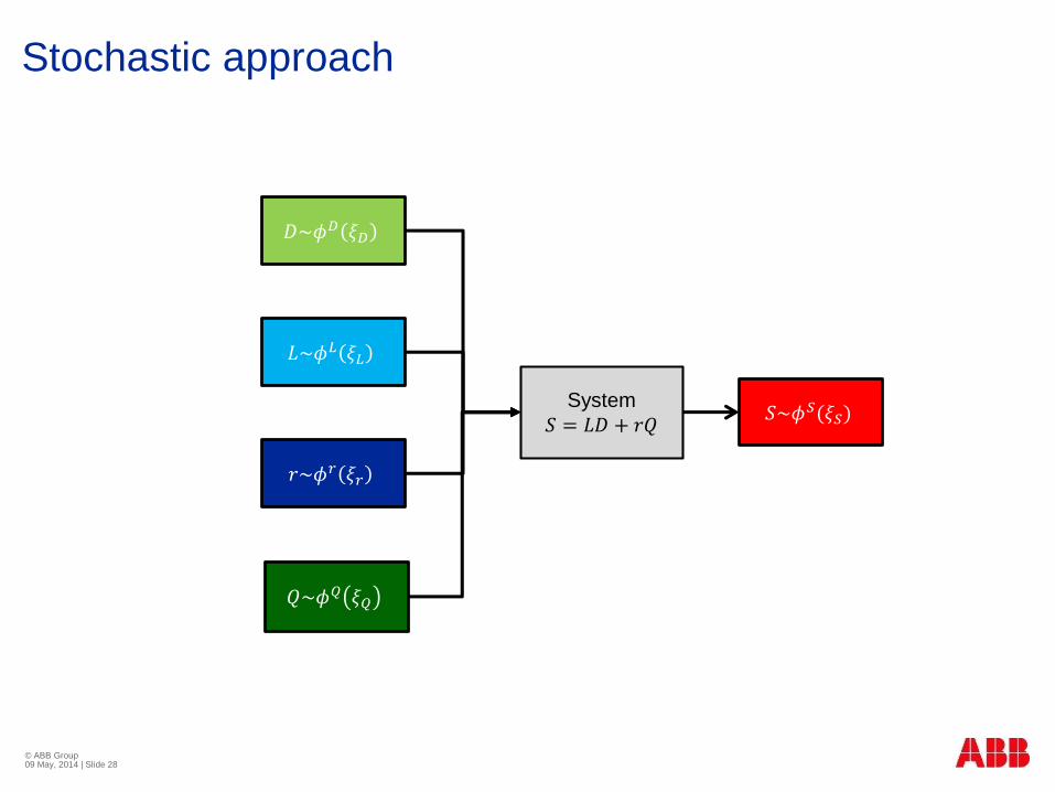
Stochastic approach
© ABB Group 09 May, 2014 | Slide 28
System
𝑆 = 𝐿𝐷 + 𝑟𝑄𝑆~𝜙𝑆(𝜉𝑆)
𝐷~𝜙𝐷 𝜉𝐷
𝐿~𝜙𝐿 𝜉𝐿
𝑟~𝜙𝑟 𝜉𝑟
𝑄~𝜙𝑄 𝜉𝑄
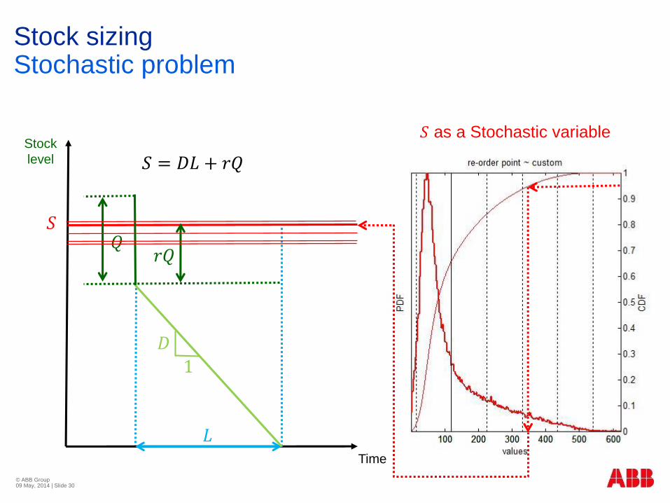
Stock sizingStochastic problem
© ABB Group 09 May, 2014 | Slide 30
Time
Stock
level
𝐿
𝑆 = 𝐷𝐿 + 𝑟𝑄
𝑆
𝑆 as a Stochastic variable
𝑄𝑟𝑄
𝐷
1
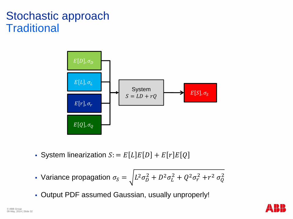
Stochastic approachTraditional
System linearization 𝑆:= 𝐸 𝐿 𝐸 𝐷 + 𝐸 𝑟 𝐸 𝑄
Variance propagation 𝜎𝑆 = 𝐿2𝜎𝐷2 + 𝐷2𝜎𝐿
2 + 𝑄2𝜎𝑟2 +𝑟2 𝜎𝑄
2
Output PDF assumed Gaussian, usually unproperly!
© ABB Group 09 May, 2014 | Slide 32
System
𝑆 = 𝐿𝐷 + 𝑟𝑄
𝐸 𝑟 , 𝜎𝑟
𝐸 𝑆 , 𝜎𝑆
𝐸 𝐷 , 𝜎𝐷
𝐸 𝐿 , 𝜎𝐿
𝐸 𝑄 , 𝜎𝑄
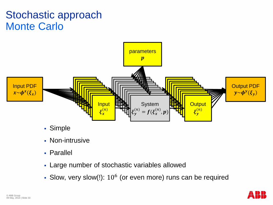
Stochastic approachMonte Carlo
Simple
Non-intrusive
Parallel
Large number of stochastic variables allowed
Slow, very slow(!): 106 (or even more) runs can be required
© ABB Group 09 May, 2014 | Slide 33
parameters
𝒑
System
𝑦𝑛 = 𝑓(𝑥𝑛)Input
𝑥𝑛
Output
𝑦𝑛
Output PDF
𝒚~𝝓𝒚(𝝃𝒚)Input PDF
𝒙~𝝓𝒙(𝝃𝒙)System
𝑦𝑛 = 𝑓(𝑥𝑛)Input
𝑥𝑛
Output
𝑦𝑛System
𝑦𝑛 = 𝑓(𝑥𝑛)Input
𝑥𝑛
Output
𝑦𝑛System
𝑦𝑛 = 𝑓(𝑥𝑛)Input
𝑥𝑛
Output
𝑦𝑛System
𝑦𝑛 = 𝑓(𝑥𝑛)Input
𝑥𝑛
Output
𝑦𝑛System
𝑦𝑛 = 𝑓(𝑥𝑛)Input
𝑥𝑛
Output
𝑦𝑛System
𝑦𝑛 = 𝑓(𝑥𝑛)Input
𝑥𝑛
Output
𝑦𝑛System
𝑦𝑛 = 𝑓(𝑥𝑛)Input
𝑥𝑛
Output
𝑦𝑛System
𝑦𝑛 = 𝑓(𝑥𝑛)Input
𝑥𝑛
Output
𝑦𝑛System
𝝃𝒚(𝑛)
= 𝒇(𝝃𝒙(𝑛)
, 𝒑)
Input
𝝃𝒙(𝑛)
Output
𝝃𝒚(𝑛)
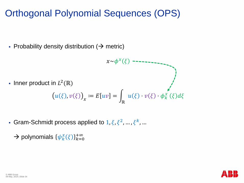
Orthogonal Polynomial Sequences (OPS)
Probability density distribution ( metric)
𝑥~𝜙𝑥 𝜉
Inner product in 𝐿2(ℝ)
𝑢 𝜉 , 𝑣 𝜉𝑥≔ 𝐸 𝑢𝑣 =
ℝ
𝑢 𝜉 ⋅ 𝑣 𝜉 ⋅ 𝜙𝑘𝑥 𝜉 𝑑𝜉
Gram-Schmidt process applied to 1, 𝜉, 𝜉2, … , 𝜉𝑘 , …
polynomials 𝜓𝑘𝑥 𝜉 𝑘=0
+∞
© ABB Group 09 May, 2014 | Slide 34
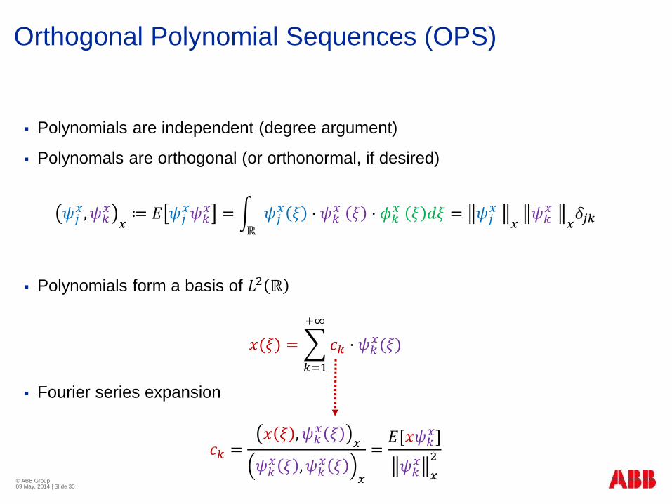
Orthogonal Polynomial Sequences (OPS)
Polynomials are independent (degree argument)
Polynomals are orthogonal (or orthonormal, if desired)
𝜓𝑗𝑥, 𝜓𝑘
𝑥
𝑥≔ 𝐸 𝜓𝑗
𝑥𝜓𝑘𝑥 =
ℝ
𝜓𝑗𝑥 𝜉 ⋅ 𝜓𝑘
𝑥 𝜉 ⋅ 𝜙𝑘𝑥 𝜉 𝑑𝜉 = 𝜓𝑗𝑘
𝑥
𝑥𝜓𝑘𝑗
𝑥
𝑥
𝑗𝛿𝑗𝑘
Polynomials form a basis of 𝐿2 ℝ
𝑥(𝜉) =
𝑘=1
+∞
𝑐𝑘 ⋅ 𝜓𝑘𝑥(𝜉)
Fourier series expansion
𝑐𝑘 =𝑥 𝜉 , 𝜓𝑘
𝑥 𝜉𝑥
𝜓𝑘𝑥 𝜉 , 𝜓𝑘
𝑥 𝜉𝑥
=𝐸[𝑥𝜓𝑘
𝑥]
𝜓𝑘𝑥
𝑥
2
© ABB Group 09 May, 2014 | Slide 35
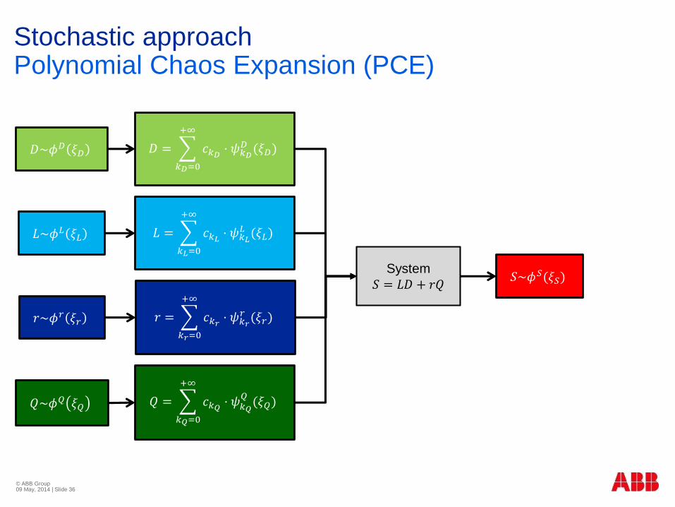
Stochastic approachPolynomial Chaos Expansion (PCE)
© ABB Group 09 May, 2014 | Slide 36
System
𝑆 = 𝐿𝐷 + 𝑟𝑄𝑆~𝜙𝑆(𝜉𝑆)
𝐷~𝜙𝐷 𝜉𝐷
𝐿~𝜙𝐿 𝜉𝐿
𝑟~𝜙𝑟 𝜉𝑟
𝑄~𝜙𝑄 𝜉𝑄
𝐷 =
𝑘𝐷=0
+∞
𝑐𝑘𝐷 ⋅ 𝜓𝑘𝐷𝐷 (𝜉𝐷)
𝐿 =
𝑘𝐿=0
+∞
𝑐𝑘𝐿 ⋅ 𝜓𝑘𝐿𝐿 (𝜉𝐿)
𝑟 =
𝑘𝑟=0
+∞
𝑐𝑘𝑟 ⋅ 𝜓𝑘𝑟𝑟 (𝜉𝑟)
𝑄 =
𝑘𝑄=0
+∞
𝑐𝑘𝑄 ⋅ 𝜓𝑘𝑄
𝑄(𝜉𝑄)
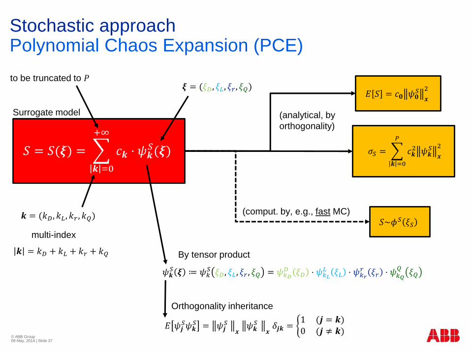
Stochastic approachPolynomial Chaos Expansion (PCE)
© ABB Group 09 May, 2014 | Slide 37
𝑆~𝜙𝑆 𝜉𝑆
𝑆 = 𝑆(𝝃) =
𝒌 =0
+∞
𝑐𝒌 ⋅ 𝜓𝒌𝑆(𝝃)
𝒌 = (𝑘𝐷, 𝑘𝐿 , 𝑘𝑟 , 𝑘𝑄)
𝝃 = (𝜉𝐷, 𝜉𝐿 , 𝜉𝑟 , 𝜉𝑄)
𝜓𝒌𝑆 𝝃 ≔ 𝜓𝑘
𝑆 𝜉𝐷, 𝜉𝐿 , 𝜉𝑟 , 𝜉𝑄 = 𝜓𝑘𝐷𝐷 𝜉𝐷 ⋅ 𝜓𝑘𝐿
𝐿 𝜉𝐿 ⋅ 𝜓𝑘𝑟𝑟 𝜉𝑟 ⋅ 𝜓𝑘𝑄
𝑄𝜉𝑄
𝒌 = 𝑘𝐷 + 𝑘𝐿 + 𝑘𝑟 + 𝑘𝑄
multi-index
to be truncated to 𝑃
𝐸 𝜓𝒋𝑆𝜓𝒌
𝑆 = 𝜓𝒋𝑘𝑆
𝒙𝜓𝒌𝑗
𝑆
𝒙𝛿𝒋𝒌 =
1 (𝒋 = 𝒌)0 (𝒋 ≠ 𝒌)
(comput. by, e.g., fast MC)
𝐸 𝑆 = 𝑐𝟎 𝜓𝟎𝑆
𝒙
2
𝜎𝑆 =
𝒌 =0
𝑃
𝑐𝒌2 𝜓𝒌
𝑆𝒙
2
Surrogate model
By tensor product
Orthogonality inheritance
(analytical, by
orthogonality)
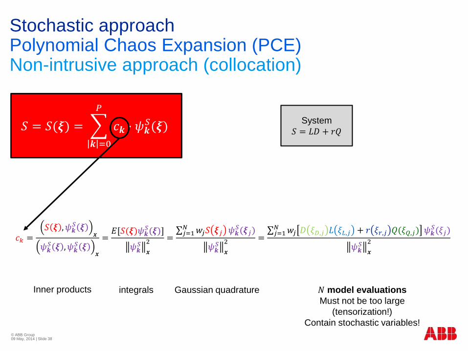
𝑐𝑘 =𝑆 𝝃 ,𝜓𝒌
𝑆 𝝃𝒙
𝜓𝒌𝑆 𝝃 ,𝜓𝒌
𝑆 𝝃𝒙
=𝐸[𝑆(𝝃)𝜓𝒌
𝑆(𝝃)]
𝜓𝒌𝑆
𝒙
2 = 𝑗=1𝑁 𝑤𝑗𝑆 𝝃𝑗 𝜓𝒌
𝑆(𝝃𝑗)
𝜓𝒌𝑆
𝒙
2 = 𝑗=1𝑁 𝑤𝑗 𝐷 𝜉𝐷,𝑗 𝐿 𝜉𝐿,𝑗 + 𝑟 𝜉𝑟,𝑗 𝑄(𝜉𝑄,𝑗) 𝜓𝒌
𝑆(𝜉𝑗)
𝜓𝒌𝑆
𝒙
2
Stochastic approachPolynomial Chaos Expansion (PCE)Non-intrusive approach (collocation)
© ABB Group 09 May, 2014 | Slide 38
𝑆 = 𝑆(𝝃) =
𝒌 =0
𝑃
𝑐𝒌 ⋅ 𝜓𝒌𝑆(𝝃)
Inner products integrals Gaussian quadrature 𝑁 model evaluations
Must not be too large
(tensorization!)
Contain stochastic variables!
System
𝑆 = 𝐿𝐷 + 𝑟𝑄
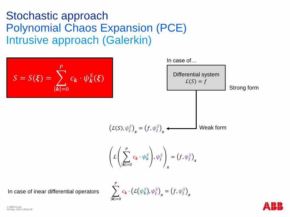
Stochastic approachPolynomial Chaos Expansion (PCE)Intrusive approach (Galerkin)
© ABB Group 09 May, 2014 | Slide 39
𝑆 = 𝑆(𝝃) =
𝒌 =0
𝑃
𝑐𝒌 ⋅ 𝜓𝒌𝑆(𝝃)
Differential system
ℒ(𝑆) = 𝑓
ℒ 𝑆 ,𝜓𝒋𝑆
𝒙= 𝑓, 𝜓𝒋
𝑆
𝒙
ℒ
𝒌 =0
𝑃
𝑐𝒌 ⋅ 𝜓𝒌𝑆 , 𝜓𝒋
𝑆
𝒙
= 𝑓,𝜓𝒋𝑆
𝒙
𝒌 =0
𝑃
𝑐𝒌 ⋅ ℒ 𝜓𝒌𝑆 , 𝜓𝒋
𝑆
𝒙= 𝑓, 𝜓𝒋
𝑆
𝒙
Strong form
Weak form
In case of inear differential operators
In case of…
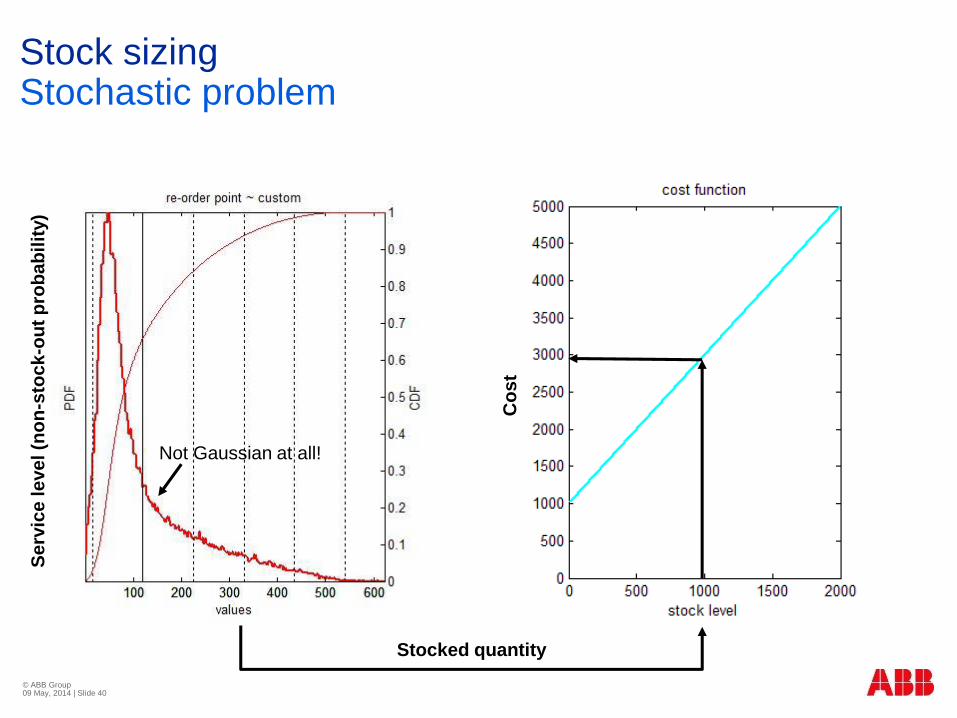
Stock sizingStochastic problem
© ABB Group 09 May, 2014 | Slide 40
Not Gaussian at all!
Co
st
Stocked quantity
Se
rvic
e le
ve
l (n
on
-sto
ck
-ou
t p
rob
ab
ilit
y)
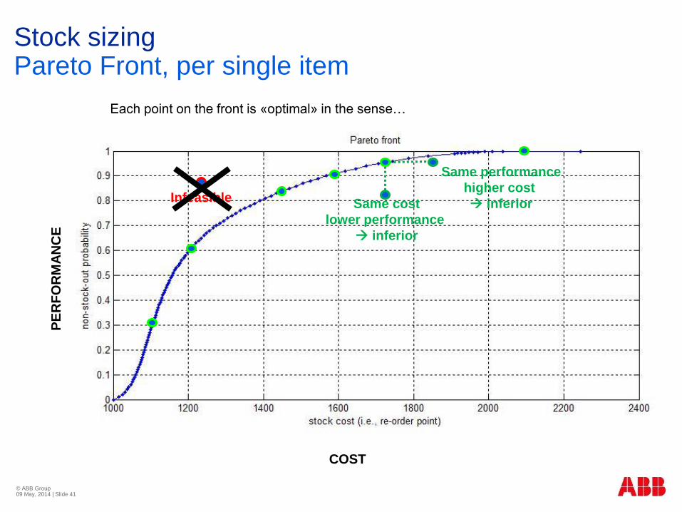
Stock sizingPareto Front, per single item
© ABB Group 09 May, 2014 | Slide 41
COST
PE
RF
OR
MA
NC
E
Same performance
higher cost
inferiorSame cost
lower performance
inferior
Each point on the front is «optimal» in the sense…
Infeasible
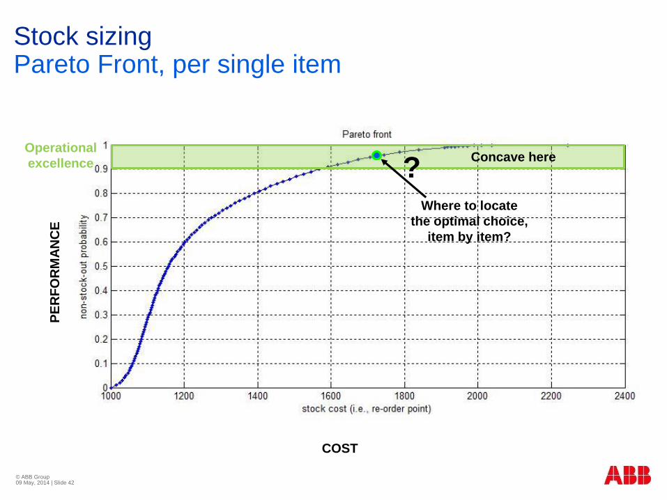
Stock sizingPareto Front, per single item
© ABB Group 09 May, 2014 | Slide 42
COST
PE
RF
OR
MA
NC
E
Concave hereOperational
excellence
Where to locate
the optimal choice,
item by item?
?
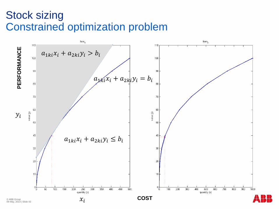
Stock sizingConstrained optimization problem
© ABB Group 09 May, 2014 | Slide 43
𝑥𝑖
𝑦𝑖
COST
PE
RF
OR
MA
NC
E
𝑖-th item
𝑎1𝑘𝑖𝑥𝑖 + 𝑎2𝑘𝑖𝑦𝑖 = 𝑏𝑖
𝑎1𝑘𝑖𝑥𝑖 + 𝑎2𝑘𝑖𝑦𝑖 > 𝑏𝑖
𝑎1𝑘𝑖𝑥𝑖 + 𝑎2𝑘𝑖𝑦𝑖 ≤ 𝑏𝑖
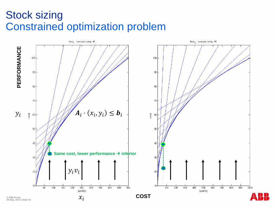
Stock sizingConstrained optimization problem
© ABB Group 09 May, 2014 | Slide 44
𝑨𝑖 ⋅ 𝑥𝑖 , 𝑦𝑖 ≤ 𝒃𝑖
𝑦𝑖𝑣𝑖
Same cost, lower performance inferior
𝑥𝑖
𝑦𝑖
COST
PE
RF
OR
MA
NC
E

Stock sizingConstrained optimization problem
© ABB Group 09 May, 2014 | Slide 45
𝑨𝑖 ⋅ 𝑥𝑖 , 𝑦𝑖 ≤ 𝒃𝑖
Same performance, higher cost inferior
𝑥𝑖
𝑦𝑖
COST
PE
RF
OR
MA
NC
E
𝑥𝑖𝑤𝑖
Stock sizingConstrained optimization problem
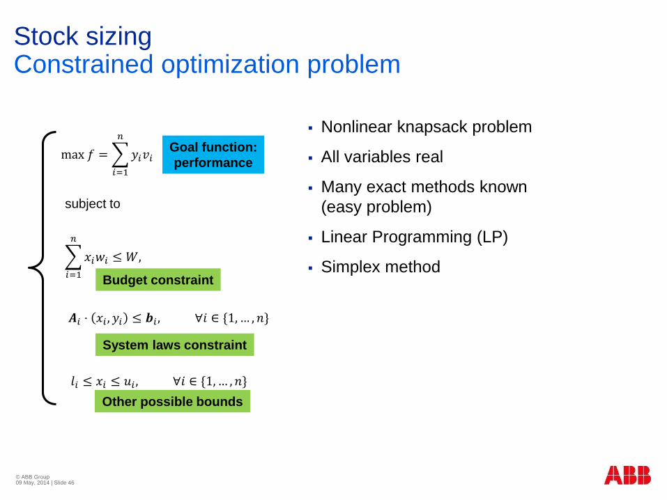
© ABB Group 09 May, 2014 | Slide 46
max 𝑓 =
𝑖=1
𝑛
𝑦𝑖𝑣𝑖
𝑖=1
𝑛
𝑥𝑖𝑤𝑖 ≤ 𝑊,
subject to
𝑙𝑖 ≤ 𝑥𝑖 ≤ 𝑢𝑖 , ∀𝑖 ∈ {1,… , 𝑛}
𝑨𝑖 ⋅ 𝑥𝑖 , 𝑦𝑖 ≤ 𝒃𝑖 , ∀𝑖 ∈ {1,… , 𝑛}
Nonlinear knapsack problem
All variables real
Many exact methods known
(easy problem)
Linear Programming (LP)
Simplex methodBudget constraint
Other possible bounds
System laws constraint
Goal function:
performance
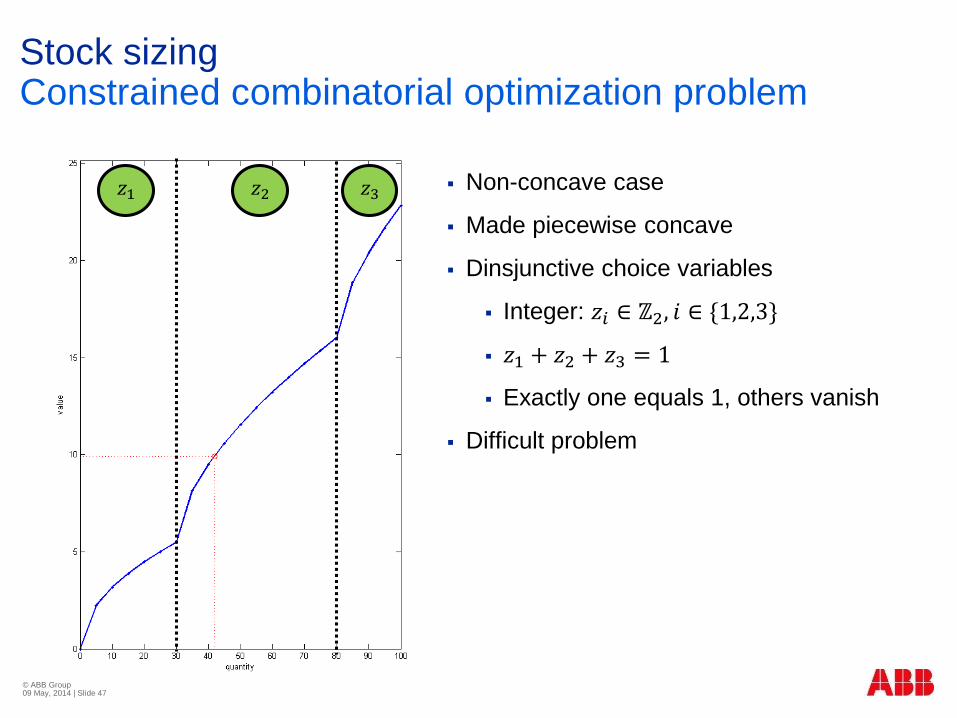
Stock sizingConstrained combinatorial optimization problem
Non-concave case
Made piecewise concave
Dinsjunctive choice variables
Integer: 𝑧𝑖 ∈ ℤ2, 𝑖 ∈ {1,2,3}
𝑧1 + 𝑧2 + 𝑧3 = 1
Exactly one equals 1, others vanish
Difficult problem
© ABB Group 09 May, 2014 | Slide 47
𝑧1 𝑧2 𝑧3
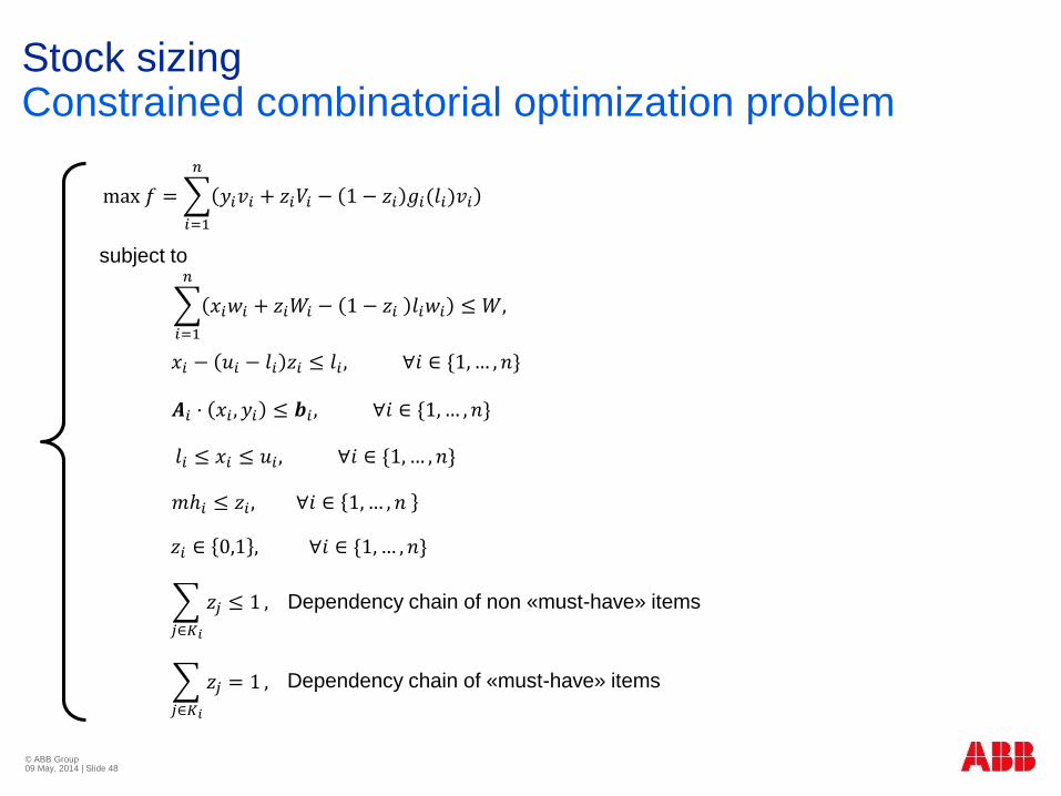
Stock sizingConstrained combinatorial optimization problem
© ABB Group 09 May, 2014 | Slide 48
max 𝑓 =
𝑖=1
𝑛
𝑦𝑖𝑣𝑖 + 𝑧𝑖𝑉𝑖 − 1 − 𝑧𝑖 𝑔𝑖(𝑙𝑖)𝑣𝑖
𝑖=1
𝑛
𝑥𝑖𝑤𝑖 + 𝑧𝑖𝑊𝑖 − 1 − 𝑧𝑖 𝑙𝑖𝑤𝑖 ≤ 𝑊,
subject to
𝑙𝑖 ≤ 𝑥𝑖 ≤ 𝑢𝑖 , ∀𝑖 ∈ {1,… , 𝑛}
𝑧𝑖 ∈ 0,1 , ∀𝑖 ∈ {1,… , 𝑛}
𝑨𝑖 ⋅ 𝑥𝑖 , 𝑦𝑖 ≤ 𝒃𝑖 , ∀𝑖 ∈ {1,… , 𝑛}
𝑗∈𝐾𝑖
𝑧𝑗 ≤ 1 ,
𝑚ℎ𝑖 ≤ 𝑧𝑖 , ∀𝑖 ∈ 1,… , 𝑛
𝑥𝑖 − 𝑢𝑖 − 𝑙𝑖 𝑧𝑖 ≤ 𝑙𝑖 , ∀𝑖 ∈ {1,… , 𝑛}
𝑗∈𝐾𝑖
𝑧𝑗 = 1 ,
Dependency chain of non «must-have» items
Dependency chain of «must-have» items

© ABBMay, 2014 | Slide 76
Future Research Trends
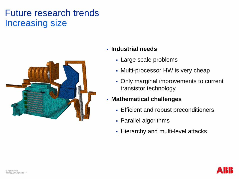
Future research trendsIncreasing size
Industrial needs
Large scale problems
Multi-processor HW is very cheap
Only marginal improvements to current
transistor technology
Mathematical challenges
Efficient and robust preconditioners
Parallel algorithms
Hierarchy and multi-level attacks
© ABB Group 09 May, 2014 | Slide 77
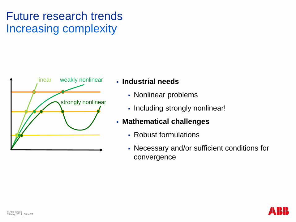
Future research trendsIncreasing complexity
Industrial needs
Nonlinear problems
Including strongly nonlinear!
Mathematical challenges
Robust formulations
Necessary and/or sufficient conditions for
convergence
© ABB Group 09 May, 2014 | Slide 78
linear weakly nonlinear
strongly nonlinear
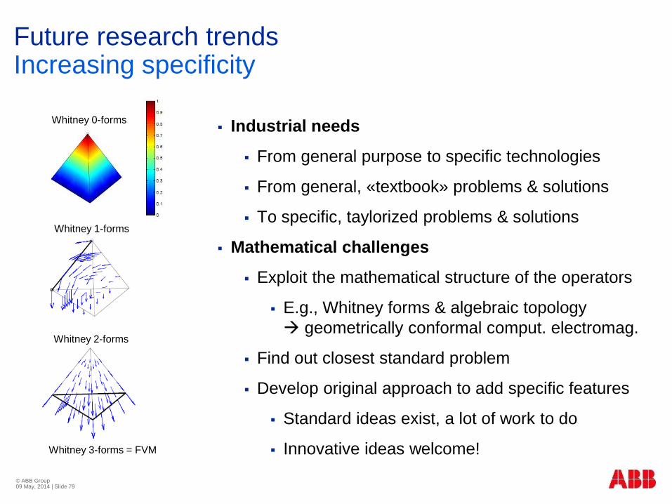
Future research trendsIncreasing specificity
Industrial needs
From general purpose to specific technologies
From general, «textbook» problems & solutions
To specific, taylorized problems & solutions
Mathematical challenges
Exploit the mathematical structure of the operators
E.g., Whitney forms & algebraic topology
geometrically conformal comput. electromag.
Find out closest standard problem
Develop original approach to add specific features
Standard ideas exist, a lot of work to do
Innovative ideas welcome!
© ABB Group 09 May, 2014 | Slide 79
Whitney 0-forms
Whitney 1-forms
Whitney 2-forms
Whitney 3-forms = FVM
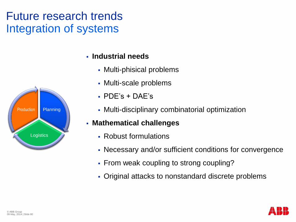
Future research trendsIntegration of systems
Industrial needs
Multi-phisical problems
Multi-scale problems
PDE’s + DAE’s
Multi-disciplinary combinatorial optimization
Mathematical challenges
Robust formulations
Necessary and/or sufficient conditions for convergence
From weak coupling to strong coupling?
Original attacks to nonstandard discrete problems
© ABB Group 09 May, 2014 | Slide 80
CFD
MECH
EMAG Planning
Logistics
Production
Future research trendsStochastics
Industrial needs
Stochastic differential equations (SDE)
Non-deterministic problems and/or boundary conditions
Either intrinsically (finance, markets, etc.)
Or de facto (e.g., deterministic PDE with non
completely known material properties or forcing terms)
Mathematical challenges
Beyond MonteCarlo & non-intrusive, black-box attacks
«Stochastic dimensions» added to physical dimensions
Preconditioners, robustness, convergence, etc.
Pure mathematics as well!
«Large» number (> 10) of stochastic variables
© ABB Group 09 May, 2014 | Slide 81
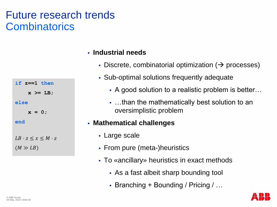
Future research trendsCombinatorics
Industrial needs
Discrete, combinatorial optimization ( processes)
Sub-optimal solutions frequently adequate
A good solution to a realistic problem is better…
…than the mathematically best solution to an
oversimplistic problem
Mathematical challenges
Large scale
From pure (meta-)heuristics
To «ancillary» heuristics in exact methods
As a fast albeit sharp bounding tool
Branching + Bounding / Pricing / …
© ABB Group 09 May, 2014 | Slide 82
if z==1 then
x >= LB;
else
x = 0;
end
𝐿𝐵 ⋅ 𝑧 ≤ 𝑥 ≤ 𝑀 ⋅ 𝑧
(𝑀 ≫ 𝐿𝐵)

© ABB Group 09 May, 2014 | Slide 83