Embed Size (px)
Citation preview
Proceedings of the 2015 Winter Simulation ConferenceL. Yilmaz, W. K. V. Chan, I. Moon, T. M. K. Roeder, C. Macal, and M. D. Rossetti, eds.
EFFICIENT SIMULATION FOR BRANCHING LINEAR RECURSIONS
Ningyuan ChenMariana Olvera-Cravioto
Industrial Engineering and Operations ResearchColumbia University
New York, NY 10027, USA
ABSTRACT
We provide an algorithm for simulating the unique attracting fixed-point of linear branching distributionalequations. Such equations appear in the analysis of information ranking algorithms, e.g., PageRank, and inthe complexity analysis of divide and conquer algorithms, e.g., Quicksort. The naive simulation approachwould be to simulate exactly a suitable number of generations of a weighted branching process, whichhas exponential complexity in the number of generations being sampled. Instead, we propose an iterativebootstrap algorithm that has linear complexity; we prove its convergence and the consistency of a familyof estimators based on our approach.
1 INTRODUCTION
The complexity analysis of divide and conquer algorithms such as Quicksort (Rosler 1991, Fill and Janson2001, Rosler and Ruschendorf 2001) and the more recent analysis of information ranking algorithms oncomplex graphs (e.g., Google’s PageRank) (Volkovich and Litvak 2010, Jelenkovic and Olvera-Cravioto2010, Chen, Litvak, and Olvera-Cravioto 2014) motivate the analysis of the stochastic fixed-point equation
R D= Q+
N
∑r=1
CrRr, (1)
where (Q,N,C1,C2, . . .) is a real-valued random vector with N ∈ N, and {Ri}i∈N is a sequence of i.i.d.copies of R, independent of (Q,N,C1,C2, . . .). More precisely, the number of comparisons required inQuicksort for sorting an array of length n, properly normalized, satisfies in the limit as the array’s lengthgrows to infinity a distributional equation of the form in (1). In the context of ranking algorithms, it hasbeen shown that the rank of a randomly chosen node in a large directed graph with n nodes converges indistribution, as the size of the graph grows, to R, where N represents the in-degree of the chosen node andthe {Ci}i≥1 are functions of the out-degree and node attributes of its neighbors. In the complexity analysisof algorithms, knowing the distribution of R makes it possible to estimate the moments and tail probabilitiesof the number of operations required to sort a list of numbers, which is important for benchmarking andworst case analysis. In the case of information ranking algorithms, the distribution of R can be used todetermine what type of nodes are typically ranked highly, which in turn can be used to design new rankingalgorithms capable of identifying pre-specified data attributes.
As further motivation for the study of branching fixed-point equations, we mention the closely relatedmaximum equation
R D= Q∨
N∨r=1
CrRr, (2)
Chen and Olvera-Cravioto
with (Q,N,C1,C2, . . .) nonnegative, which has been shown to appear in the analysis of the waiting timedistribution in large queueing networks with parallel servers and synchronization requirements (Karpelevich,Kelbert, and Suhov 1994, Olvera-Cravioto and Ruiz-Lacedelli 2014). In this setting, W = logR representsthe waiting time in stationarity of a job, that upon arrival to the network, is split into a number of subtasksrequiring simultaneous service from a random subset of servers. Computing the distribution and themoments of W is hence important for evaluating the performance of such systems (e.g., implementationsof MapReduce and similar algorithms in today’s cloud computing). Due to length limitations, we focus inthis paper only on (1), but we mention that the algorithm we provide can easily be adapted to approximatelysimulate the solutions to (2) (see Remark 2).
Although the study of (1) and (2), and other max-plus branching recursions, has received considerableattention in the recent years (Rosler 1991, Biggins 1998, Fill and Janson 2001, Rosler and Ruschendorf 2001,Aldous and Bandyopadhyay 2005, Alsmeyer, Biggins, and Meiners 2012, Alsmeyer and Meiners 2012,Alsmeyer and Meiners 2013, Jelenkovic and Olvera-Cravioto 2012b, Jelenkovic and Olvera-Cravioto 2012a,Jelenkovic and Olvera-Cravioto 2015), the current literature only provides results on the characterizationof the solutions to (1) and (2), their tail asymptotics, and in some instances, their integer moments, whichis not always enough for the applications mentioned above. It is therefore of practical importance to havea numerical approach to estimate both the distribution and the general moments of R.
As a mathematical observation, we mention that both (1) and (2) are known to have multiple solutions(see e.g. Biggins (1998), Alsmeyer, Biggins, and Meiners (2012), Alsmeyer and Meiners (2012), Alsmeyerand Meiners (2013) and the references therein for the characterization of the solutions). However, inapplications we are often interested in the so-called endogenous solution. This endogenous solution is theunique limit under iterations of the distributional recursion
R(k+1) D=
N
∑r=1
CrR(k)r +Q, (3)
where (Q,N,C1,C2, . . .) is a real-valued random vector with N ∈ N, and {R(k)i }i∈N is a sequence of i.i.d.
copies of R(k), independent of (Q,N,C1,C2, . . .), provided one starts with an initial distribution for R(0) withsufficient finite moments (see, e.g., Lemma 4.5 in Jelenkovic and Olvera-Cravioto (2012a)). Moreover,asymptotics for the tail distribution of the endogenous solution R are available under several different sets ofassumptions for (Q,N,C1,C2, . . .) (Jelenkovic and Olvera-Cravioto 2010, Jelenkovic and Olvera-Cravioto2012b, Jelenkovic and Olvera-Cravioto 2012a, Olvera-Cravioto 2012).
As will be discussed later, the endogenous solution to (1) can be explicitly constructed on a weightedbranching process. Thus, drawing some similarities with the analysis of branching processes, and theGalton-Watson process in particular, one could think of using the Laplace transform of R to obtain itsdistribution. Unfortunately, the presence of the weights {Ci} in the Laplace transform
ϕ(s) = E [exp(−sR)] = E
[exp(−sQ)
N
∏i=1
ϕ(sCi)
]makes its inversion problematic, making a simulation approach even more necessary.
The first observation we make regarding the simulation of R, is that when P(Q = 0)< 1 it is enoughto be able to approximate R(k) for fixed values of k, since both R(k) and R can be constructed in the sameprobability space in such a way that the difference |R(k)−R| is geometrically small. More precisely, undervery general conditions (see Proposition 1 in Section 2), there exist positive constants K < ∞ and c < 1such that
E[∣∣∣R(k)−R
∣∣∣β]≤ Kck+1. (4)
Our goal is then to simulate R(k) for a suitably large value of k.
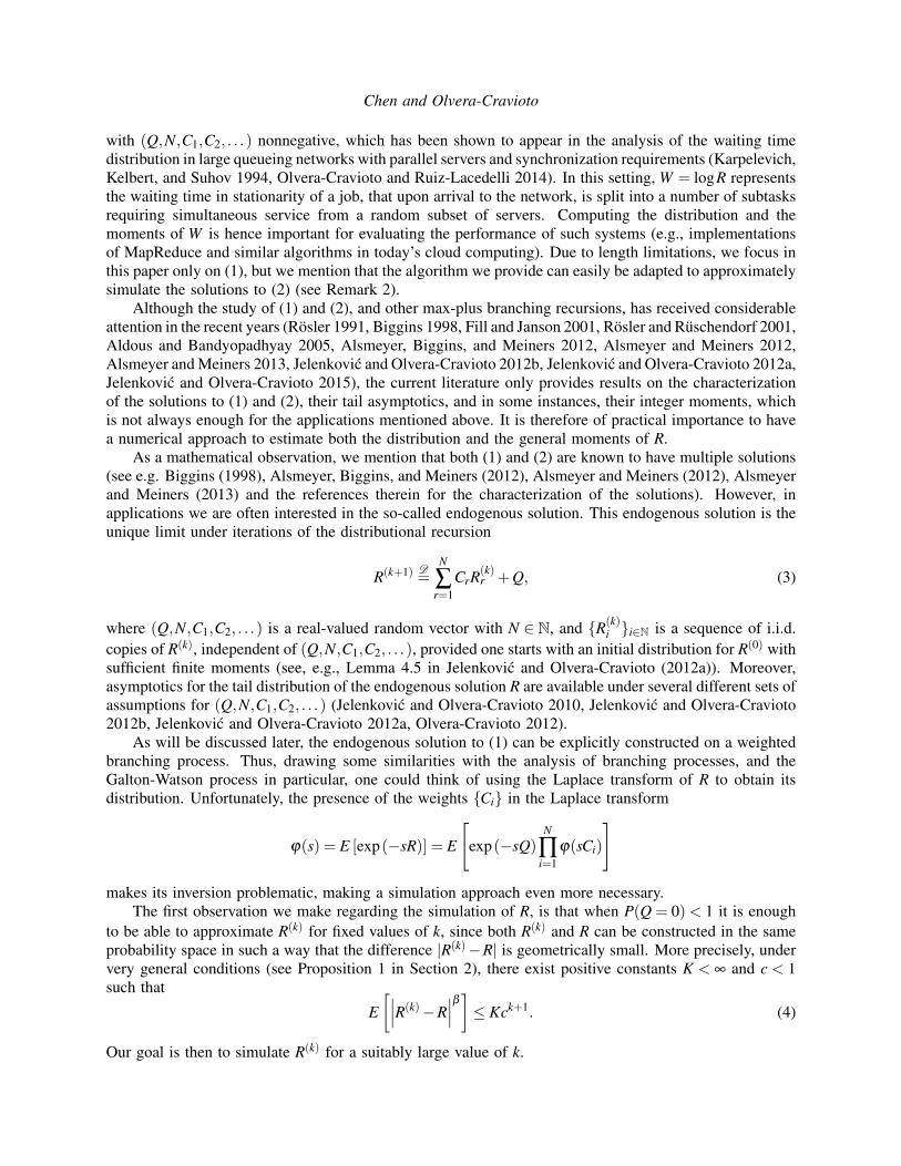
Chen and Olvera-Cravioto
Π /0 = 1
Π1 =C1 Π2 =C2 Π3 =C3
Π(1,1) =C(1,1)C1
Π(1,2) =C(1,2)C1
Π(2,1) =C(2,1)C2
Π(3,1) =C(3,1)C3
Π(3,2) =C(3,2)C3
Π(3,3) =C(3,3)C3
Figure 1: Weighted branching process
The simulation of R(k) is not that straightforward either, since the naive approach of simulating i.i.d.copies of (Q,N,C1,C2, . . .) to construct a single realization of a weighted branching process, up to sayk generations, is of order (E[N])k. Considering that in the examples mentioned earlier we typically haveE[N] > 1 (N ≡ 2 for Quicksort, E[N] ≈ 30 in many information ranking applications, and E[N] in thehundreds for MapReduce implementations), this approach is prohibitive. Instead, we propose in this paperan iterative bootstrap algorithm that outputs a sample pool of observations {R(k,m)
i }mi=1 whose empirical
distribution converges, in the Kantorovich-Rubinstein distance, to that of R(k) as the size of the pool m→∞.This mode of convergence is equivalent to weak convergence and convergence of the first absolute moments(see, e.g., Villani (2009)). Moreover, the complexity of our proposed algorithm is linear in k. This algorithmis known in the statistical physics literature as “population dynamics” (see, e.g., Mezard and Montanari(2009)), where it has been used heuristically for the approximation of belief propagation algorithms.
The paper is organized as follows. Section 2 describes the weighted branching process and the linearrecursion. The algorithm itself is given in Section 3, which includes a remark on how to adapt it to themaximum case. Section 4 introduces the Kantorovich-Rubinstein distance and proves the convergenceproperties of our proposed algorithm. Numerical examples to illustrate the precision of the algorithm arepresented in Section 5.
2 LINEAR RECURSIONS ON WEIGHTED BRANCHING PROCESSES
As mentioned in the introduction, the endogenous solution to (1) can be explicitly constructed on a weightedbranching process. To describe the structure of a weighted branching process, let N+ = {1,2,3, . . .} bethe set of positive integers and let U =
⋃∞k=0(N+)
k be the set of all finite sequences i = (i1, i2, . . . , in),n≥ 0, where by convention N0
+ = { /0} contains the null sequence /0. To ease the exposition, we will use(i, j) = (i1, . . . , in, j) to denote the index concatenation operation.
Next, let (Q,N,C1,C2, . . .) be a real-valued vector with N ∈ N. We will refer to this vector as thegeneric branching vector. Now let {(Qi,Ni,C(i,1),C(i,2), . . .)}i∈U be a sequence of i.i.d. copies of the genericbranching vector. To construct a weighted branching process we start by defining a tree as follows: letA0 = { /0} denote the root of the tree, and define the nth generation according to the recursion
An = {(i, in) ∈U : i ∈ An−1,1≤ in ≤ Ni}, n≥ 1.
Now, assign to each node i in the tree a weight Πi according to the recursion
Π /0 ≡ 1, Π(i,in) =C(i,in)Πi, n≥ 1,
see Figure 1. If P(N < ∞) = 1 and Ci ≡ 1 for all i ≥ 1, the weighted branching process reduces to aGalton-Watson process.
Chen and Olvera-Cravioto
For a weighted branching process with generic branching vector (Q,N,C1,C2, . . .), define the process{R(k) : k ≥ 0} as follows:
R(k) =k
∑j=0
∑i∈A j
QiΠi, k ≥ 0. (5)
By focusing on the branching vector belonging to the root node, i.e., (Q /0,N/0,C1,C2, . . .) we can see thatthe process {R(k)} satisfies the distributional equations
R(0) = Q /0D= Q
R(k) = Q /0 +N/0
∑r=1
Cr
(k
∑j=1
∑(r,i)∈A j
Q(r,i)Π(r,i)/Cr
)D= Q+
N
∑r=1
CrR(k−1)r , k ≥ 1, (6)
where R(k−1)r are i.i.d. copies of R(k−1), all independent of (Q,N,C1,C2, . . .). Here and throughout the
paper the convention is that XY/Y ≡ 1 if Y = 0. Moreover, if we define
R =∞
∑j=0
∑i∈A j
QiΠi, (7)
we have the following result. We use x∨ y to denote the maximum of x and y.
Proposition 1 Let β ≥ 1 be such that E[|Q|β ]< ∞ and E[(
∑Ni=1 |Ci|
)β]< ∞. In addition, assume either
(i) (ρ1 ∨ρβ ) < 1 , or (ii) β = 2, ρ1 = 1, ρβ < 1 and E[Q] = 0. Then, there exist constants Kβ > 0 and0 < cβ < 1 such that for R(k) and R defined according to (5) and (7), respectively, we have
supk≥0
E[|R(k)|β
]≤ Kβ < ∞ and E
[|R(k)−R|β
]≤ Kβ ck+1
β.
Proof. For the case ρ1∨ρβ < 1, Lemma 4.4 in Jelenkovic and Olvera-Cravioto (2012a) gives that forWn = ∑i∈An QiΠi and some finite constant Hβ we have
E[|Wn|β
]≤ Hβ (ρ1∨ρβ )
n.
Let cβ = ρ1∨ρβ . Minkowski’s inequality then gives
∣∣∣∣∣∣R(k)∣∣∣∣∣∣
β
≤k
∑n=0||Wn||β ≤
∞
∑n=0
(Hβ cn
β
)1/β
=
Hβ
1− c1/β
β
1/β
,(Kβ
)1/β< ∞.
Similarly,
∣∣∣∣∣∣R(k)−R∣∣∣∣∣∣
β
≤∞
∑n=k+1
||Wn||β ≤∞
∑n=k+1
(Hβ cn
β
)1/β
= c(k+1)/β
β
(Hβ
1− (ρ1∨ρβ )1/β
)1/β
=(
Kβ ck+1β
)1/β
.
For the case β = 2, ρ1 = 1, ρβ < 1 and E[Q] = 0 we have that
E[W 2
n]= E
( N/0
∑r=1
CrWn−1,r
)2= E
[N/0
∑r=1
C2r (Wn−1,r)
2 + ∑1≤r 6=s≤N/0
CrCsWn−1,rWn−1,s
],
Chen and Olvera-Cravioto
where Wn−1,r = ∑(r,i)∈An Q(r,i)Π(r,i)/Cr, and the {Wn−1,r}r≥1 are i.i.d. copies of Wn−1, independent of(N/0,C1,C2, . . .). Since E[Wn] = 0 for all n≥ 0, it follows that
E[W 2n ] = ρ2E[W 2
n−1] = ρn2 E[W 2
0 ] = Var(Q)ρn2 .
The two results now follow from the same arguments used above with H2 = Var(Q) and c2 = ρ2.
It follows from the previous result that under the conditions of Proposition 1, R(k) converges to R bothalmost surely and in Lβ -norm. Similarly, if we ignore the Q in the generic branching vector, assume thatCi ≥ 0 for all i, and define the process
W (k) = ∑i∈Ak
Πi =N/0
∑r=1
Cr
(∑
(r,i)∈Ak
Π(r,i)/Cr
)D=
N
∑r=1
CrW(k−1)r ,
where the {W (k−1)r }r≥1 are i.i.d. copies of W (k−1) independent of (N,C1,C2, . . .), then it can be shown
that {W (k)/ρk1 : k≥ 0} defines a nonnegative martingale which converges almost surely to the endogenous
solution of the stochastic fixed-point equation
W D=
N
∑i=1
Ci
ρ1Wi,
where the {Wi}i≥1 are i.i.d. copies of W , independent of (N,C1,C2, . . .). We refer to this equation as thehomogeneous case.
As mentioned in the introduction, our objective is to generate a sample of R(k) for values of k sufficientlylarge to suitably approximate R. Our proposed algorithm can also be used to simulate W (k), but due tospace limitations we will omit the details.
3 THE ALGORITHM
Note that based on (5), one way to simulate R(k) would be to simulate a weighted branching process startingfrom the root and up to the k generation and then add all the weights QiΠi for i ∈⋃k
j=0 A j. Alternatively,we could generate a large enough pool of i.i.d. copies of Q which would represent the Qi for i ∈ Ak, anduse them to generate a pool of i.i.d. observations of R(1) by setting
R(1)i =
Ni
∑r=1
C(i,r)R(0)r +Qi,
where {(Qi,Ni,C(i,1),C(i,2), . . .)}i≥1 are i.i.d. copies of the generic branching vector, independent of
everything else, and the R(0)r are the Q’s generated in the previous step. We can continue this process
until we get to the root node. On average, we would need (E[N])k i.i.d. copies of Q for the first poolof observations, (E[N])k−1 copies of the generic branching vector for the second pool, and in general,(E[N])k− j for the jth step. This approach is equivalent to simulating the weighted branching processstarting from the kth generation and going up to the root, and is the result of iterating (3).
Our proposed algorithm is based on this “leaves to root” approach, but to avoid the need for a geometricnumber of “leaves”, we will resample from the initial pool to obtain a pool of the same size of observationsof R(1). In general, for the jth generation we will sample from the pool obtained in the previous stepof (approximate) observations of R( j−1) to obtain conditionally independent (approximate) copies of R( j).In other words, to obtain a pool of approximate copies of R( j) we bootstrap from the pool previouslyobtained of approximate copies of R( j−1). The approximation lies in the fact that we are not sampling from
Chen and Olvera-Cravioto
R( j−1) itself, but from a finite sample of conditionally independent observations that are only approximatelydistributed as R( j−1). The algorithm is described below.
Let (Q,N,C1,C2, . . .) denote the generic branching vector defining the weighted branching process.Let k be the depth of the recursion that we want to simulate, i.e., the algorithm will produce a sample ofrandom variables approximately distributed as R(k). Choose m ∈ N+ to be the bootstrap sample size. Foreach 0≤ j≤ k, the algorithm outputs P( j,m) ,
(R( j,m)
1 , R( j,m)2 , . . . , R( j,m)
m
), which we refer to as the sample
pool at level j.
1. Initialize: Set j = 0. Simulate a sequence {Qi}mi=1 of i.i.d. copies of Q and let R(0,m)
i = Qi for
i = 1, . . . ,m. Output P(0,m) =(
R(0,m)1 , R(0,m)
2 , . . . , R(0,m)m
)and update j = 1.
2. While j ≤ k:(a) Simulate a sequence {(Qi,Ni,C(i,1),C(i,2), . . .)}m
i=1 of i.i.d. copies of the generic branchingvector, independent of everything else.
(b) Let
R( j,m)i = Qi +
Ni
∑r=1
C(i,r)R( j−1,m)(i,r) , i = 1, . . . ,m, (8)
where the R( j−1,m)(i,r) are sampled uniformly with replacement from the pool P( j−1,m).
(c) Output P( j,m) =(
R( j,m)1 , R( j,m)
2 , . . . , R( j,m)m
)and update j = j+1.
Remark 2 To simulate an approximation for the endogenous solution to the maximum equation (2), givenby R =
∨∞j=0∨
i∈A jQiΠi, simply replace (8) with
R( j,m)i = Qi∨
Ni∨r=1
C(i,r)R( j−1,m)(i,r) , i = 1, . . . ,m.
Bootstrapping refers broadly to any method that relies on random sampling with replacement (Efronand Tibshirani 1993). For example, bootstrapping can be used to estimate the variance of an estimator, byconstructing samples of the estimator from a number of resamples of the original dataset with replacement.With the same idea, our algorithm draws samples uniformly with replacement from the previous bootstrapsample pool. Therefore, the R( j−1,m)
(i,r) on the right-hand side of (8) are only conditionally independent given
P( j−1,m). Hence, the samples in P( j,m) are identically distributed but not independent for j ≥ 1.As we mentioned earlier, the distribution of the {R( j,m)
i } in P( j,m) are only approximately distributedas R( j), with the exception of the {R(0,m)
i } which are exact. The first thing that we need to prove isthat the distribution of the observations in P( j,m) does indeed converge to that of R( j). Intuitively, thisshould be the case since the empirical distribution of the {R(0,m)
i } is the empirical distribution of m i.i.d.observations of R(0), and therefore should be close to the true distribution of R(0) for suitably large m.Similarly, since the {R(1,m)
i } are constructed by sampling from the empirical distribution of P(0,m), whichis close to the true distribution of R(0), then their empirical distribution should be close to the empiricaldistribution of R(1), which in turn should be close to the true distribution of R(1). Inductively, providedthe approximation is good in step j−1, we can expect the empirical distribution of P( j,m) to be close tothe true distribution of R( j). In the following section we make the mode of the convergence precise byconsidering the Kantorovich-Rubinstein distance between the empirical distribution of P( j,m) and the truedistribution of R( j).

Chen and Olvera-Cravioto
The second technical aspect of our proposed algorithm is the lack of independence among the observationsin P(k,m), since a natural estimator for quantities of the form E[h(R(k))] would be to use
1m
m
∑i=1
h(R(k,m)i ). (9)
Hence, we also provide a result establishing the consistency of estimators of the form in (9) for a suitablefamily of functions h.
We conclude this section by pointing out that the complexity of the algorithm described above is oforder km, while the naive Monte Carlo approach described earlier, which consists on sampling m i.i.d.copies of a weighted branching process up to the kth generation, has order (E[N])km. This is a huge gainin efficiency.
4 CONVERGENCE AND CONSISTENCY
In order to show that our proposed algorithm does indeed produce observations that are approximatelydistributed as R(k) for any fixed k, we will show that the empirical distribution function of the observationsin P(k,m) , i.e.,
Fk,m(x) =1m
m
∑i=1
1(R(k,m)i ≤ x)
converges as m→ ∞ to the true distribution function of R(k), which we will denote by Fk. We will showthis by using the Kantorovich-Rubinstein distance, which is a metric on the space of probability measures.In particular, convergence in this sense is equivalent to weak convergence plus convergence of the firstabsolute moments.Definition 1 let M(µ,ν) denote the set of joint probability measures on R×R with marginals µ and ν .then, the Kantorovich-Rubinstein distance between µ and ν is given by
d1(µ,ν) = infπ∈M(µ,ν)
∫R×R|x− y|dπ(x,y).
We point out that d1 is only strictly speaking a distance when both µ and ν have finite first absolutemoments. Moreover, it is well known that
d1(µ,ν) =∫ 1
0|F−1(u)−G−1(u)|du =
∫∞
−∞
|F(x)−G(x)|dx. (10)
where F and G are the cumulative distribution functions of µ and ν , respectively, and f−1(t) = inf{x ∈R : f (x) ≥ t} denotes the pseudo-inverse of f . It follows that the optimal coupling of two real randomvariables X and Y is given by (X ,Y ) = (F−1(U),G−1(U)), where U is uniformly distributed in [0,1].Remark 3 The Kantorovich-Rubinstein distance is also known as the Wasserstein metric of order 1. Ingeneral, both the Kantorovich-Rubinstein distance and the more general Wasserstein metric of order p canbe defined in any metric space; we restrict our definition in this paper to the real line since that is all weneed. We refer the interested reader to (Villani 2009) for more details.
With some abuse of notation, for two distribution functions F and G we use d1(F,G) to denote theKantorovich-Rubinstein distance between their corresponding probability measures.
The following proposition shows that for i.i.d. samples, the expected value of the Kantorovich-Rubinsteindistance between the empirical distribution function and the true distribution converges to zero.Proposition 4 Let {Xi}i≥1 be a sequence of i.i.d. random variables with common distribution F . Let Fndenote the empirical distribution function of a sample of size n. Then, provided there exists α ∈ (1,2)
Chen and Olvera-Cravioto
such that E [|X1|α ]< ∞, we have that
E [d1(Fn,F)]≤ n−1+1/α
(2α
α−1+
22−α
)E[|X1|α ].
Proposition 4 can be proved following the same arguments used in the proof of Theorem 2.2 in delBarrio, Gine, and Matran (1999) by setting M = 1, and thus we omit it.
We now give the main theorem of the paper, which establishes the convergence of the expectedKantorovich-Rubinstein distance between Fk,m and Fk. Its proof is based on induction and the explicitrepresentation (10). Recall that ρβ = E
[∑
Ni=1 |Ci|β
].
Theorem 5 Suppose that the conditions of Proposition 1 are satisfied for some β > 1. Then, for anyα ∈ (1,2) with α ≤ β , there exists a constant Kα < ∞ such that
E[d1(Fk,m,Fk)
]≤ Kαm−1+1/α
k
∑i=0
ρi1. (11)
Proof. By Proposition 1 there exists a constant Hα such that
Hα = supk≥0
E[|R(k)|α
]≤ sup
k≥0
(E[|R(k)|β
])α/β
< ∞.
Set Kα = Hα
( 2α
α−1 +2
2−α
). We will give a proof by induction.
For j = 0, we have that F0,m(x) = 1m ∑
mi=1 1(Qi ≤ x), where {Qi}i≥1 is a sequence of i.i.d. copies of Q.
It follows that F0,m is the empirical distribution function of R(0), and by Proposition 4 we have that
E[d1(F0,m,F0)
]≤ Kαm−1+1/α .
Now suppose that (11) holds for j− 1. Let {U ir}i,r≥1 be a sequence of i.i.d. Uniform(0,1) random
variables, independent of everything else. Let {(Qi,Ni,C(i,1),C(i,2), . . .)}i≥1 be a sequence of i.i.d. copiesof the generic branching vector, also independent of everything else. Recall that Fj−1 is the distributionfunction of R( j−1) and define the random variables
R( j,m)i =
Ni
∑r=1
C(i,r)F−1j−1,m(U
ir)+Qi and R( j)
i =Ni
∑r=1
C(i,r)F−1j−1(U
ir)+Qi
for each i = 1,2, . . . ,m. Now use these random variables to define
Fj,m(x) =1m
m
∑i=1
1(R( j,m)i ≤ x) and Fj,m(x) =
1m
m
∑i=1
1(R( j)i ≤ x).
Note that Fj,m is an empirical distribution function of i.i.d. copies of R( j), which has been carefully coupledwith the function Fj,m produced by the algorithm.
By the triangle inequality and Proposition 4 we have that
E[d1(Fj,m,Fj)
]≤ E
[d1(Fj,m,Fj,m)
]+E [d1(Fj,m,Fj)]≤ E
[d1(Fj,m,Fj,m)
]+Kαm−1+1/α .
To analyze the remaining expectation note that
E[d1(Fj,m,Fj,m)
]= E
[∫∞
−∞
|Fj,m(x)−Fj,m(x)|dx]≤ 1
m
m
∑i=1
E[∫
∞
−∞
∣∣∣1(R( j,m)i ≤ x)−1(R( j)
i ≤ x)∣∣∣dx]
=1m
m
∑i=1
E[∣∣∣R( j,m)
i −R( j)i
∣∣∣]= 1m
m
∑i=1
E
[∣∣∣∣∣ Ni
∑r=1
C(i,r)(F−1j−1,m(U
ir)−F−1
j−1(Uir))
∣∣∣∣∣]
≤ E
[N
∑r=1|Cr|]
E[d1(Fj−1,m,Fj−1)
],
Chen and Olvera-Cravioto
where in the last step we used the fact that (Ni,C(i,1),C(i,2), . . .) is independent of{
U ir}
r≥1 and of Fj−1,m,combined with the explicit representation of the Kantorovich-Rubinstein distance given in (10). Theinduction hypothesis now gives
E[d1(Fj,m,Fj)
]≤ ρ1E
[d1(Fj−1,m,Fj−1)
]+Kαm−1+1/α ≤ Kαm−1+1/α
ρ1
j−1
∑i=0
ρi1 +Kαm−1+1/α
= Kαm−1+1/α
j
∑i=0
ρi1.
This completes the proof.
Note that the proof of Theorem 5 implies that R( j,m)i → R( j)
i =∑Nir=1C(i,r)F
−1j−1(U
ir)+Qi
D= R( j) in L1-norm
for all fixed j ∈ N, and hence in distribution. In other words,
P(
R(k,m)i ≤ x
)→ Fk(x) as m→ ∞, (12)
for all i = 1,2, . . . ,m, and for any continuity point of Fk. This also implies that
E[Fk,m(x)
]= P
(R(k,m)
1 ≤ x)→ Fk(x) as m→ ∞, (13)
for all continuity points of Fk.Since our algorithm produces a pool P(k,m) of m random variables approximately distributed according
to Fk, it makes sense to use it for estimating expectations related to R(k). In particular, we are interestedin estimators of the form in (9). The problem with this kind of estimators is that the random variables inP(k,m) are only conditionally independent given Fk−1,m.
Definition 2 We say that Θn is a consistent estimator for θ if ΘnP→ θ as n→ ∞, where P→ denotes
convergence in probability.Our second theorem shows the consistency of estimators of the form in (9) for a broad class of functions.
Theorem 6 Suppose that the conditions of Proposition 1 are satisfied for some β > 1. Suppose h : R→Ris continuous and |h(x)| ≤C(1+ |x|) for all x ∈ R and some constant C > 0. Then, the estimator
1m
m
∑i=1
h(R(k,m)i ) =
∫R
h(x)dFk,m(x),
where P(k,m) =(
R(k,m)1 , R(k,m)
2 , . . . , R(k,m)m
), is a consistent estimator for E[h(R(k))].
Proof. For any M > 0, define hM(x) as
hM(x) = h(−M)1(x≤−M)+h(x)1(−M < x≤M)+h(M)1(x > M),
and note that hM is uniformly continuous. We then have∣∣∣∣∫R h(x)dFk,m(x)−∫R
h(x)dFk(x)∣∣∣∣≤ 2C
∫|x|>M
(1+ |x|)dFk(x)+2C∫|x|>M
(1+ |x|)dFk,m(x)
+
∣∣∣∣∫R hM(x)dFk,m(x)−∫R
hM(x)dFk(x)∣∣∣∣ . (14)

Chen and Olvera-Cravioto
Fix ε > 0 and choose Mε > 0 such that E[(|R(k)|+1)1(|R(k)|> Mε)
]≤ ε/(4C) and such that −Mε and Mε
are continuity points of Fk. Define (R(k,m),R(k)) = (F−1k,m(U),F−1
k (U)), where U is a uniform [0,1] randomvariable independent of P(k,m). Next, note that g(x) = 1+ |x| is Lipschitz continuous with Lipschitzconstant one and therefore∫|x|>Mε
(1+ |x|)dFk,m(x) = (1+Mε)(Fk,m(−Mε)+1− Fk,m(Mε)
)+∫
x<−Mε
Fk,m(x)dx+∫
x>Mε
(1− Fk,m(x))dx
≤ (1+Mε)(Fk,m(−Mε)+1− Fk,m(Mε)
)+d1(Fk,m,Fk)
+∫
x<−Mε
Fk(x)dx+∫
x>Mε
(1−Fk(x))dx
= (1+Mε)(Fk,m(−Mε)−Fk(−Mε)+Fk(Mε)− Fk,m(Mε)
)+d1(Fk,m,Fk)
+E[(|R(k)|+1)1(|R(k)|> Mε)
].
Finally, since hMεis bounded and uniformly continuous, then ω(δ ) = sup{|hMε
(x)−hMε(y)| : |x−y| ≤ δ}
converges to zero as δ → 0. Hence, for any γ > 0,∣∣∣∣∫R hMε(x)dFk,m(x)−
∫R
hMε(x)dFk(x)
∣∣∣∣≤ E[∣∣∣hMε
(R(k,m))−hMε(R(k))
∣∣∣∣∣∣ Fk,m
]≤ ω(m−γ)+KεE
[1(|R(k,m)−R(k)|> m−γ
)∣∣∣ Fk,m
]≤ ω(m−γ)+Kεmγd1(Fk,m,Fk),
where 2Kε = sup{|hMε(x)| : x ∈R}. Choose 0 < γ < 1−1/α for the α ∈ (1,2) in Theorem 5 and combine
the previous estimates to obtain
E[∣∣∣∣∫R h(x)dFk,m(dx)−
∫R
h(x)dFk(dx)∣∣∣∣]≤ 2C(1+Mε)
(E[Fk,m(−Mε)]−Fk(−Mε)+Fk(Mε)−E[Fk,m(Mε)]
)+ ε +ω(m−γ)+(2C+Kεmγ)E
[d1(Fk,m,Fk)
].
Since E[Fk,m(−Mε)]→ Fk(−Mε) and E[Fk,m(Mε)]→ Fk(Mε) by (13), and mγE[d1(Fk,m,Fk)
]→ 0 by The-
orem 5, it follows that
limsupm→∞
E[∣∣∣∣∫R h(x)dFk,m(dx)−
∫R
h(x)dFk(dx)∣∣∣∣]≤ ε.
Since ε > 0 was arbitrary, the convergence in L1, and therefore in probability, follows.
5 NUMERICAL EXAMPLES
This last section of the paper gives a numerical example to illustrate the performance of our algorithm.Consider a generic branching vector (Q,N,C1,C2, . . .) where the {Ci}i≥1 are i.i.d. and independent of Nand Q, with N also independent of Q.
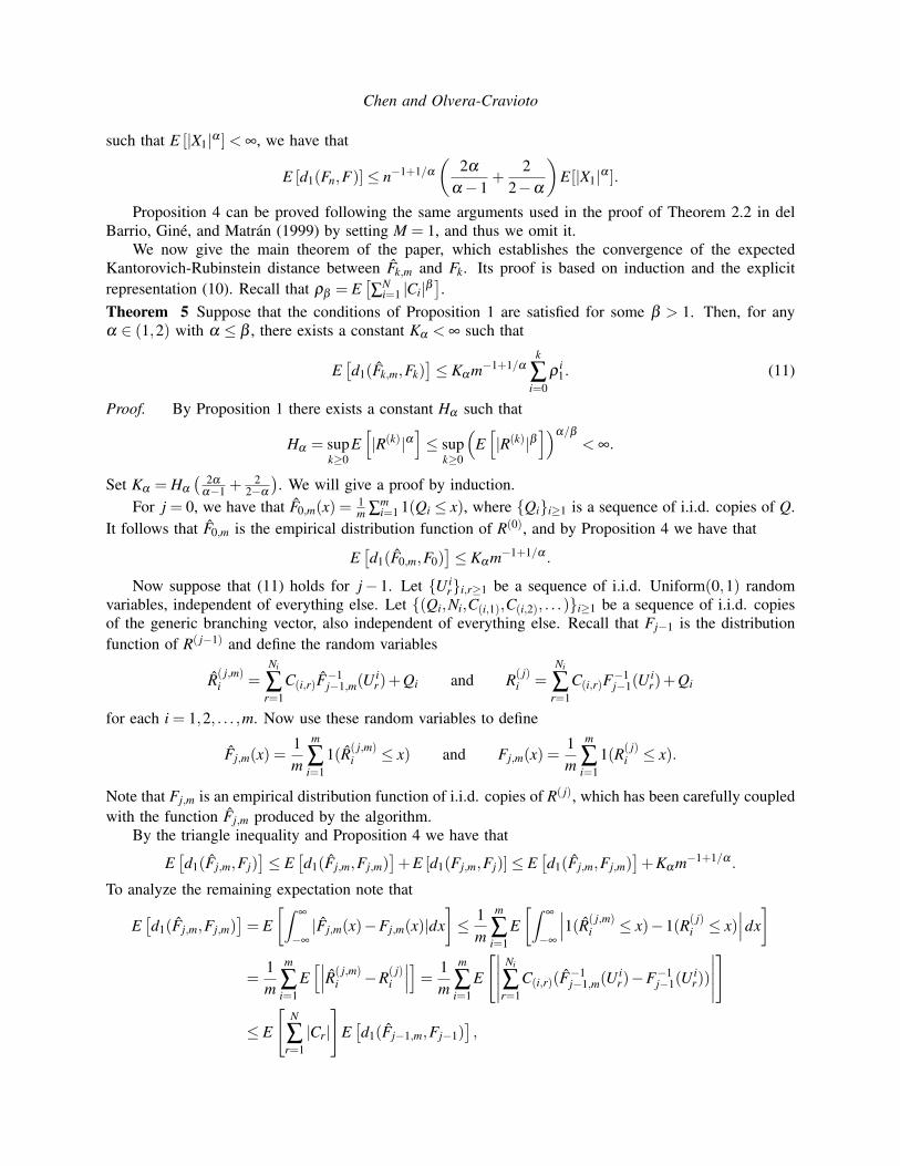
Figure 2a plots the empirical cumulative distribution function of 1000 samples of R(10, i.e., F10,1000 inour notation, versus the functions F10,200 and F10,1000 produced by our algorithm, for the case where the Ciare uniformly distributed in [0,0.2], Q uniformly distributed in [0,1] and N is a Poisson random variablewith mean 3. Note that we cannot compare our results with the true distribution F10 since it is not availablein closed form. Computing F10,1000 required 883.3 seconds using Python with an Intel i7-4700MQ 2.40GHz processor and 8 GB of memory, while computing F10,1000 required only 2.1 seconds. We point out

Chen and Olvera-Cravioto
0 0.5 1 1.5 20
0.2
0.4
0.6
0.8
1
x
F10,1000
F10,1000
F10,200
(a) The functions F10,1000(x), F10,200(x) andF10,1000(x).
5 10 15 20 25 30 35 400
1
2
3
4·10−2
x
1− F10,10000
1− F10,10000
G10
(b) The functions 1−F10,10000(x), 1− F10,10000(x)and G10(x), where G10 is evaluated only at integervalues of x and linearly interpolated in between.
Figure 2: Numerical examples.
that in applications to information ranking algorithms E[N] can be in the thirties range, which would makethe difference in computation time even more impressive.
Our second example plots the tail distribution of the empirical cumulative distribution function of R(10)
for 10,000 samples versus the tail of F10,10000 for an example where N is a zeta random varialbe with aprobability mass function P(N = k) ∝ k−2.5, Q is an exponential random variable with mean 1, and theCi have a uniform distribution in [0,0.5]. In this case the exact asymptotics for P(R(k) > x) as x→ ∞ aregiven by
P(R(k) > x)∼ (E[C1]E[Q])α
(1−ρ1)α
k
∑j=0
ρj
α(1−ρk− j1 )αP(N > x),
where P(N > x) = x−αL(x) is regularly varying (see Lemma 5.1 in Jelenkovic and Olvera-Cravioto (2010)),which reduces for the specific distributions we have chosen to
G10(x),(0.25)2.5
(1− (0.49))2.5
10
∑j=0
(0.07) j(1− (0.49)10− j)2.5P(N > x) = (0.365)P(N > x).
Figure 2b plots the complementary distributions of F10,10000, F10,10000 and compares them to G. We cansee that the tails of both F10,10000 and F10,10000 approach the asymptotic roughly at the same time.
REFERENCES
Aldous, D., and A. Bandyopadhyay. 2005. “A Survey of Max-Type Recursive Distributional Equation”.Annals of Applied Probability 15 (2): 1047–1110.
Alsmeyer, G., J. Biggins, and M. Meiners. 2012. “The Functional Equation of the Smoothing Transform”.Ann. Probab. 40 (5): 2069–2105.
Alsmeyer, G., and M. Meiners. 2012. “Fixed Points of Inhomogeneous Smoothing Transforms”. J. Differ.Equ. Appl. 18 (8): 1287–1304.

Chen and Olvera-Cravioto
Alsmeyer, G., and M. Meiners. 2013. “Fixed points of the smoothing transform: Two-sided solutions”.Probab. Theory Rel. 155 (1-2): 165–199.
Biggins, J. 1998. “Lindley-type equations in the branching random walk”. Stochastic Process. Appl. 75:105–133.
Chen, N., N. Litvak, and M. Olvera-Cravioto. 2014. “Ranking algorithms on directed configuration networks”.ArXiv:1409.7443:1–39.
del Barrio, E., E. Gine, and C. Matran. 1999. “Central limit theorems for the Wasserstein distance betweenthe empirical and the true distributions”. Annals of Probability:1009–1071.
Efron, B., and R. J. Tibshirani. 1993. An introductin to the bootstrap.Fill, J., and S. Janson. 2001. “Approximating the limiting Quicksort distribution”. Random Structures
Algorithms 19 (3-4): 376–406.Jelenkovic, P., and M. Olvera-Cravioto. 2010. “Information ranking and power laws on trees”. Adv. Appl.
Prob. 42 (4): 1057–1093.Jelenkovic, P., and M. Olvera-Cravioto. 2012a. “Implicit Renewal Theorem for Trees with General Weights”.
Stochastic Process. Appl. 122 (9): 3209–3238.Jelenkovic, P., and M. Olvera-Cravioto. 2012b. “Implicit Renewal Theory and Power Tails on Trees”. Adv.
Appl. Prob. 44 (2): 528–561.Jelenkovic, P., and M. Olvera-Cravioto. 2015. “Maximums on Trees”. Stochastic Process. Appl. 125:217–
232.Karpelevich, F. I., M. Y. Kelbert, and Y. M. Suhov. 1994. “Higher-order Lindley equations”. Stochastic
Processes and their Applications 53 (1): 65–96.Mezard, M., and A. Montanari. 2009. Information, physics, and computation. Oxford University Press.Olvera-Cravioto, M. 2012. “Tail behavior of solutions of linear recursions on trees”. Stochastic Process.
Appl. 122 (4): 1777–1807.Olvera-Cravioto, M., and O. Ruiz-Lacedelli. 2014. “Parallel queues with synchronization”.
arXiv:1501.00186.Rosler, U. 1991. “A limit theorem for “Quicksort””. RAIRO Theor. Inform. Appl. 25:85–100.Rosler, U., and L. Ruschendorf. 2001. “The contraction method for recursive algorithms”. Algorithmica 29
(1-2): 3–33.Villani, C. 2009. Optimal transport, old and new. New York: Springer.Volkovich, Y., and N. Litvak. 2010. “Asymptotic Analysis for Personalized Web Search”. Adv. Appl. Prob. 42
(2): 577–604.
AUTHOR BIOGRAPHIES
NINGYUAN CHEN is a Ph.D. student in the IEOR Department at Columbia University. He obtained hisB.S. in Mathematics from Peking University and a M.S. in Operations Research from Columbia University.His research focuses on two areas: (1) Applied Probability, in particular, random graphs and informationranking algorithms, and (2) strategic behavior of customers under market microstructure, with interfacesof dynamic pricing, stochastic modeling and optimization. His email address is [email protected].
MARIANA OLVERA-CRAVIOTO is an Associate Professor in the IEOR Department at ColumbiaUniversity. She obtained her Ph.D. in Management Science and Engineering from Stanford University andholds an M.S. in Statistics from the same university. Her research interests are in Applied Probability,in particular, the analysis of information ranking algorithms, queueing theory, random graphs, weightedbranching processes and heavy-tailed asymptotics in general. She serves in the editorial board of StochasticModels and QUESTA. Her e-mail address is [email protected].