L4 Optical design Flow in-software and aberrations

ME 297 L4 Optical design flow

L4 Nayer Eradat

Fall 2011 SJSU

L4 ME 297 SJSU Eradat Fall 2011 1

2 L4 ME 297 SJSU Eradat Fall 2011

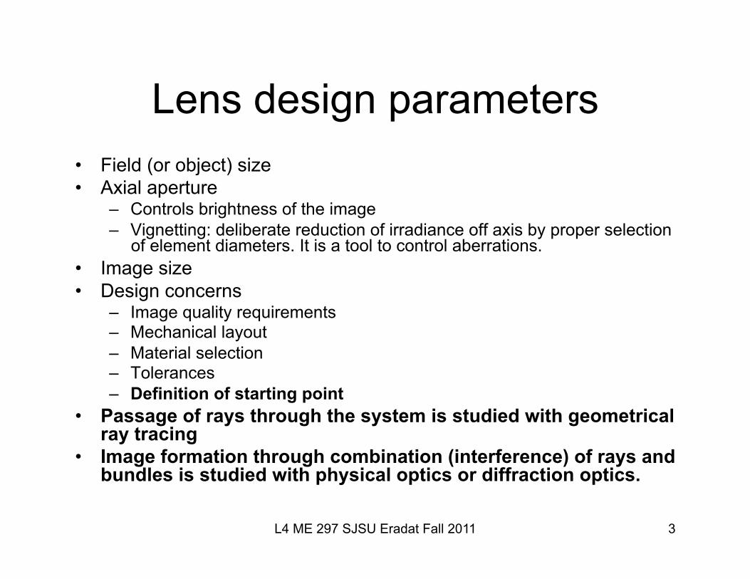
Lens design parameters •  Field (or object) size •  Axial aperture

–  Controls brightness of the image –  Vignetting: deliberate reduction of irradiance off axis by proper selection

of element diameters. It is a tool to control aberrations. •  Image size •  Design concerns

–  Image quality requirements –  Mechanical layout –  Material selection –  Tolerances –  Definition of starting point

•  Passage of rays through the system is studied with geometrical ray tracing

•  Image formation through combination (interference) of rays and bundles is studied with physical optics or diffraction optics.


Data supplied by customer

Initial selection of parameters by designer

Evaluation of parameters by designer for selection of realistic and economic requirements

Select first order optical specifications to establish paraxial base set of coordinates in which the image is evaluated

Mechanical and fabrication requirements

Select tolerances 1)  Requirements on construction

parameters 2)  The need to use the lens in a defined

environment 3)  Acceptable irregularities on the lens

surface to control absorption and scattered light

Designer perturbs the system according to these tolerances and makes sure the system still meets the specifications

Cost and schedule for delivery

1.  Focal length 2.  Weight 3.  Spectral range 4.  Image quality 5.  Number of elements 6.  Available space 7.  cost

Basic design steps


Detailed description of a lens

•  Sequentially numbered set of spherical surfaces –  Curvature –  Thickness to the next surface –  Index of refraction of the medium after the surface –  Surface shape –  Orientation –  Dimension

•  Operating condition


Merit functions used in design evaluation

Evaluation of a lens is done through sampling state of aberration of the lens by computing light distribution across the lens including diffraction effect 1.  Ray intercept plots 2.  Spot diagrams 3.  Point Spread Function (PSF) 4.  Optical transfer function (OTF) 5.  Modulation transfer function (MTF)


Designing a simple low-cost fixed-focus digital camera lens

•  A simple objective lens for a fixed-focus digital camera

•  Interpret general design specifications. •  Identify starting points based on design specs. •  Match the starting points to the requirements •  Perform basic analysis, compare results with

specs. •  Determine guidelines for optimization. •  Optimize the lens •  Identify problems for potential refinements.


Fixed-focus VGA digital camera objective specs (Ref: CODE V user guide)

•  Number of elements: 1-3 •  Material: common glasses or plastics •  Image sensor: Agilent FDCS-2020

–  Resolution: 640x480 –  Pixel size: 7.4x7.4 microns –  Sensitive area: 3.55x4.74 mm (full diagonal 6 mm)

•  Objective lens: –  Focus: fixed, depth of field 750 mm (2.5 ft) to infinity –  Focal length: fixed, 6.0 mm –  Geometric Distortion: <4% –  f/number: Fixed aperture, f/3.5 –  Sharpness: MTF through focus range (central area is inner 3 mm of CCD)

–  Vignetting: Corner relative illumination > 60% –  Transmission: Lens alone >80% 400-700 nm –  IR filter: 1 mm thick Schott IR638 or Hoya CM500

Low frequency 17 lp/mm >90% (central) >85% (outer)

High frequency, 51 lp/mm >30% (central) >25% (outer)


Interpretation of the design parameters; semi-FOV or f#

h Object height

h’ Image height

Focal length of the system (effective focal length EFL) is f = 6mm Sensor size = half of the diagonal size = h ' = 3mm.The sensor size and effective focal length (EFL) will establish the field of view (FOV )For object at ∞ the image height is : h ' = f tanθFor the image height equal to the sensor size, h ' 3mm (here):h ' = EFL × tan semi − FOV( ); EFL = 6mm

semi − FOV = tan−1 h 'EFL

⎛⎝⎜

⎞⎠⎟= tan−1 3mm

6mm⎛⎝⎜

⎞⎠⎟= 26.570

Most patent databases are listed by f / # and semi - FOV


Interpretation of the parameters II: cut-off frequency

The sensor is a CCD array of fixed-size cells called pixels.There are three colour pixels in each cell. For simplicity we assume each cell consists of one pixel. Pixel size = xpxl × ypxl = 7.4 × 7.4µ2 so fX( )max

= fY( )max

CCD cut-off ferequency: fmax =12

1xpxl

= 12

17.4 ×10−3 = 67.6 lines

mm

Any image with spatial frequency components higher than 67 lp/mm will not be seen with our CCD array.The optics should provide details beyond the cut-off frequency of the CCD so that the combined optics/detector MTF will produce usable contrast up to the CCD's cut off frequency listed in the specs.


Interpretation of the design parameters; sharpness

Sharpness or MTF quantifies the systems ability on imaging as a function of spatial frequency.

MTF fX , fY( ) = OTF = H fX , fY( ) .

Maximum limits: 0.0 ≤ MTF ≤ 1.0Spatial frequency is measurd in # of lines / mm and defines the level of details in the image. Low frequency 17 lp/mm

>90% (central) >85% (outer)

High frequency, 51 lp/mm

>30% (central) >25% (outer)


3.55

4.74

3mm

The design starting point I •  Start the software •  File>new> •  New lens wizard (if exists)>Patent lens>filter

–  Can select from expired patent database of the software. Code V offers 2456 of them

–  You can also access patent search from tools>patent lens search

•  Select the filter parameters according to the needs +/- a range so you don’t miss the design options. You can always optimize for the perfect match later. What we need is: –  f = 6 mm; a fast lens or small f/# –  semi-FOV = 26.50; and a wide FOV –  Small number of elements (1-3); a cheap lens.


The design starting point II •  How to chose among the possible options?

– Always choose the lens with a larger FOV than needed because it is easy to limit the FOV but very hard to expand the FOV

– Choose the lens with smallest F# (fastest lens) among the ones offer the needed FOV since stepping down a lens to a larger F# improves the image quality.


Entering system data •  The next is entering the system data (information about the

lens usage) –  Image f/# –  Wavelength of simulations (you can increase weight of any

wavelength to increase sensitivity for that wavelength. Make the weight 2 for the green.

–  Reference wavelength used for paraxial and reference ray-tracing (default is ok)

–  Fields lists the simulated fields angle. Usually minimum three is required 0, 0.7 and full field.

–  For wide angle lenses more than three is good. We choose 4 at 0,11,19,26.50

•  The lens data will appear after clicking next and done


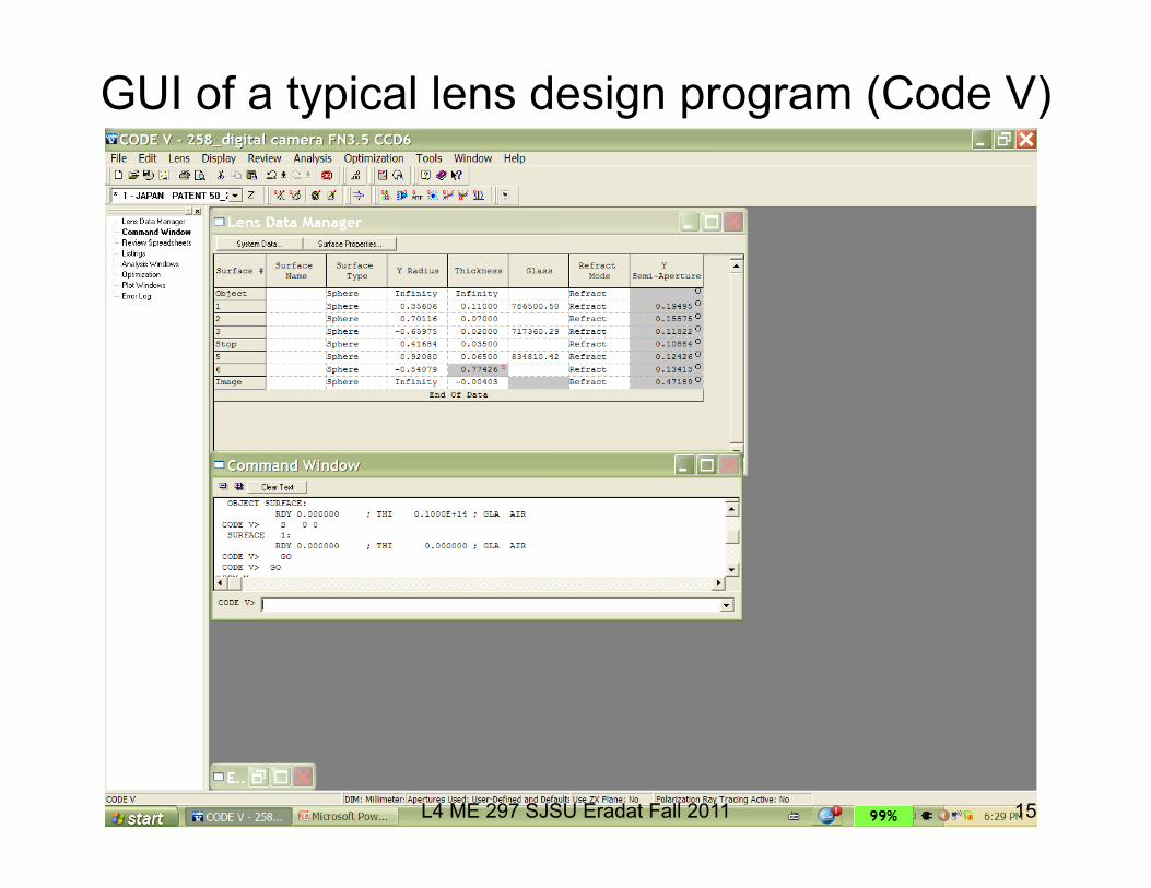
GUI of a typical lens design program (Code V)


Lens Data manager •  The basic operation of the lens design software is ray-

tracing. •  Everything else is a derivative of this operation. •  Ray tracing is done sequentially from surface to surface. •  The optical system is defined through a series of

surfaces. •  The surface and system data are listed in the lens data

manager (LDM) spreadsheet. •  The gray cells are result of calculations. •  All the data and operation related to a cell can be seen

by right clicking on it. •  Format of the cells can be changed by

tools>customize>format cells


Lens Data manager: surface data I •  All the systems will start with object surface and end with image

surface. •  Stop: is the aperture surface. The chief ray (principal ray) from

every point passes through center (x=0 & y=0) of the stop surface.

•  Surface number, Surface name, Surface type •  Y radius: (1/mm) or radius of curvature or reciprocal of

curvature, for non-spherically symmetric surfaces we have X- & Y-curvatures,

•  Thickness: distance to the next surface. Thickness of the last surface (one before the image surface) is calculated by location of the paraxial image and is done by the paraxial image (PIM) solver.

•  Location of the best focus is given from the PIM. •  Optimization determines the best focus


Lens Data manager: material & interface

•  Glass: material in the space following the surface (blank for air).

•  You can use real glass from catalog or fictitious glass with variable index for optimization. Then convert the results to a real glass that one can buy. (glassfit.seg macro in Code V does that)

•  Refract/reflect determines the basic property of the surface. •  Y Semi-Aperture represents the size of the optically useful

portion of the lens. Usually it is a circular aperture centered on the optical axis and calculated by the system but possible to change it.


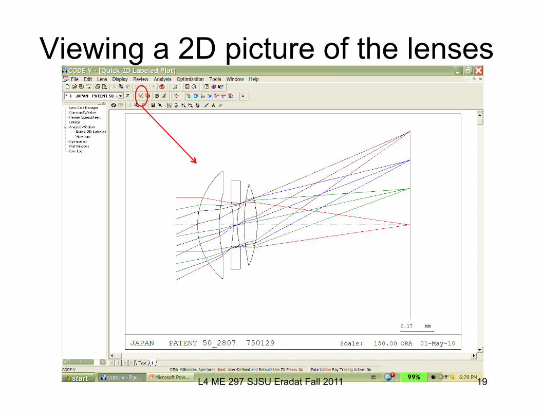
Viewing a 2D picture of the lenses


Surface operations: scale the lens •  We selected the f# and FOV but we need to make sure

the lens has the desired physical dimensions EFL=6mm. This can be done through “window of the first order properties”: –  Display>List Lens Data>First Order Data

•  If the data is different than desired we can scale the lens to bring them to what we want.

•  Highlight the surface number on the LDM and choose Edit>Scale and select scale the EFL and insert value 6.0

•  Click the execute button on the “List first order data” and “Quick 2D plot” windows to refresh them.

•  Now both EFL=6mm and image height=2.99 as desired •  Use the Lens>System data>System settings to select

title and working condition and other system parameters. 20 L4 ME 297 SJSU Eradat Fall 2011

Analyze the starting point •  Original check to see if we meet the specs •  First order requirements (focal length and Image height) •  Distortion (field curves and distortion grid) •  Sharpness (diffraction MTF) •  Depth of focus (MTF at different object distances) •  Vignetting / illumination (transmission analysis) •  Ray aberration curves •  Spot diagrams •  Establish feasibility (usually we use the existing experience to check):

–  Assume someone has to manufacture this lens or system, what practical issues will they face?

–  Size of the elements (too small /too big / too thin / too thick) –  Ease of assembling and mounting –  Price and availability of the required material (glass, etc.) –  Tolerance analysis –  Thermal analysis (usually system design software are good at this)


Ray and wave aberrations

L3 ME 297 SJSU Eradat Fall 2011

Spherical wavefront: resulting from the Gaussian or paraxial approximation.

Actual wavefront: a surface perpendicular to the sufficiently large number of the rays traced by accurarte formulas.Ray aberrations: deviations of actual rays from the ideal Gausssian rays. Longitudinal aberration: the 'miss' along the optical axis (LI ). Transverse or lateral aberration: the 'miss' on the image plane (IS).Wave aberrations: are defined based on deviations of the deformed wavefront from the ideal Gaussian wavefront at various heights from the optical axis.

In this example AB is the wave aberration.Goal of optical design: reduce the ray and wave aberrations to their unavoidable limit by diffraction.

Origin of aberrations


Sine and cosine expansion :sinφ = φ − φ3

3!+ φ5

5!+ ⋅ ⋅ ⋅

cosφ = 1− φ 2

2!+ φ 4

4!+ ⋅ ⋅ ⋅

⎧

⎨⎪⎪

⎩⎪⎪

Gaussian optics or first order optics is result of paraxial approximation which

includes only the first - order tems in sine and cosine expansions : sinφ ≅ φ cosφ ≅ 1 ⎧⎨⎩

Aberration is departure of the image from the perfect Gaussian optics image. Higher order terms in sine and cosine expansion express larger departeures from the perfect Gaussian image. Third - order aberration theory rises from inclusion of the term with third order in expansion of sine. Third - order or Seidel aberrations are result of third order aberration theory.Chromatic aberration is result of the wevelngth − dependence of the idex of refraction (or dispersion) for polychromatic light.

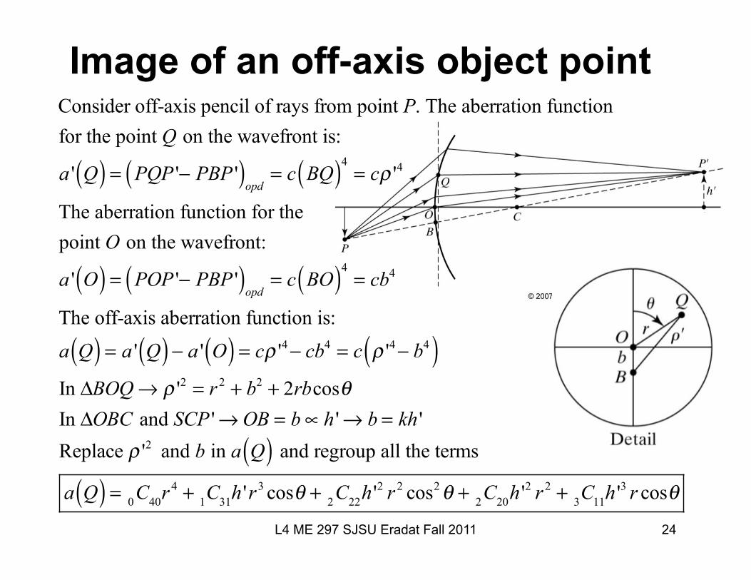
Image of an off-axis object point

Consider off-axis pencil of rays from point P. The aberration function for the point Q on the wavefront is:

a ' Q( ) = PQP '− PBP '( )opd= c BQ( )4

= cρ '4

The aberration function for the point O on the wavefront:

a ' O( ) = POP '− PBP '( )opd= c BO( )4

= cb4

The off-axis aberration function is:

a Q( ) = a ' Q( ) − a ' O( ) = cρ '4− cb4 = c ρ '4− b4( )In ΔBOQ → ρ '2 = r 2 + b2 + 2rbcosθ In ΔOBC and SCP '→ OB = b ∝ h '→ b = kh 'Replace ρ '2 and b in a Q( ) and regroup all the terms

a Q( ) = 0C40r4 + 1C31h 'r3 cosθ + 2C22h '2 r 2 cos2θ + 2C20h '2 r 2 + 3C11h '3 r cosθ


Aberration of an off-axis object point


The iC jk aberration coenfficients have indecies that are powers of the terms:

h ' : departure from axial imager : aperture of the refracting surface cosθ : azimutal angle on the aperturei is power of h ' j is power of rk is power of cosθ


Seidel aberration

Off-axis aberration functiona Q( ) = 0C40r

4 + 1C31h 'r3 cosθ + 2C22h '2 r 2 cos2θ + 2C20h '2 r 2 + 3C11h '3 r cosθ

Each term comprises one kind of monochomatic aberration or Seidel aberration as follows:

0C40r4 ← Spherical aberration (r is the system aperture).

1C31h 'r3 cosθ ← coma

2C22h' 2r 2 cos2θ ← astigmatism

2C20h' 2r 2 ← curvature of field

3C11h' 3r cosθ ← distortion


Longitudinal aberration

Transverse aberration

Spherical aberrations


0C40r4 ← Spherical aberration (r is the system aperture).

The only term independent of the h ' (departur from axial imaging) is the spherical aberration so it exists even for paraxial and axial points. The rays refracted from the extremities of the lens generate two types of spherical aberrations:

Lateral spherical: by =40C40s '

n2

r3

Longitudinal spherical: bz =40C40s '2

n2

r 2

Expressed in terms of Seidel coefficients.


Spherical aberration of the thin lenses


Longitudinal spherical aberration : miss of the ray from the paraxial image point on the optical axis (EI on the figure) For a positive lens E falls to the left of I ,

For a negative lens E falls to the right of I

Transverse spherical aberration : miss of the ray from the paraxial image point on the tansvrse plane (IG on the figure)Circle of least confusion : image of a point at the best focus point located somewhere between the paraxial image point and the image by the marginal rays, (between E and I ).

Different image distances due to spherical aberration

Different focal lengths due to spherical aberration

Coddington shape factor of a lens


f is defined for the paraxial rays in a thin lens.

As h→∞ then 1f= n −1( ) 1

r1

− 1r2

⎛

⎝⎜⎞

⎠⎟

It is possible to achieve a given f with a different combinations of r1 and r2.We define the Coddington shape factor σ as a measure of bending of a lens.

σ =r2 + r1

r2 − r1

with the usual sign convention for radii: convex +, concave − .

Example: n = 1.50 and f = 10cmσ = −2→ r1 = 10cm, r2 = 3.33cm, meniscusσ= −1→ r1 = ∞, r2 = 5cm, planoconvexσ = 0→ r1 = 10cm, r2 = −10cm, equiconvexσ=+1→ r1 = 5cm, r2 = ∞, planoconvexσ = +2→ r1 = 3.33cm, r2 = 10cm, meniscus

Minimum spherical aberration condition for bending factor


Spherical aberration of a single spherical refracting surface

a Q( ) = − h4

8n1

s1s+ 1

R⎛⎝⎜

⎞⎠⎟

2

+n2

s '1s '− 1

R⎛⎝⎜

⎞⎠⎟

2⎡

⎣⎢⎢

⎤

⎦⎥⎥

A thin lens is a combination of two such surfaces. Each surface has a contribution to the total aberration.s 'h− s 'p : total longitudinal spherical aberration

s'h : image distance for a ray at elevation hs'p : image distance for a paraxial ray

Spherical aberration of the lens is:

1s'h

− 1s 'p

= h2

8 f 3

1n n −1( )

n + 2n −1

σ 2 + 4 n +1( ) pσ + 3n + 2( ) n −1( ) p2 + n3

n −1⎡

⎣⎢

⎤

⎦⎥

Where p = s '− ss '+ s

and σ =r2 + r1

r2 − r1

is the shape factor.

Minimum spherical aberration condition for bending factor


The minimum spherical aberration results when the bending factor and p have the following relationship :

σ = −2 n2 −1( )

n + 2p where p = s '− s

s '+ s and σ =

r2 + r1

r2 − r1

For s →∞ and n = 1.50 we get bending factor σ ≅ 0.7. This is close to σ of a planoconvex lens σ=+1 with convex side facing the parallel incident rays.In general there is a possibility of cancelling spherical aberration by using two surfaces that have equal refraction with opposite signs since:

the positive and negative lenses produce spherical aberration of opposite signs.

Example of spherical aberrations

•  A point source as imaged by a system with negative (top), zero (centre), and positive (bottom) spherical aberration. Images to the left are defocused toward the inside, images on the right toward the outside (wikipedia)


+

-

+

Coma (resembles comet)

a Q( )Off-axis aberration

= ...+ 1C31h 'r3 cosθComa, an off-axial aberration

+ ...

h ' ≠ 0, and is not symmetrical about the optical axis or cosθ ≠ constantComa rapidly increases with system aperture (r3).Zone: a thin annular region of a lens centered at optical axis.Comatic circle: is created by all the rays arriving from a distant object and passing through a zone. Radius of the comatic circles increase with radius of the generating zone (figure a).


Coma (resembles comet)

a Q( )Off-axis aberration

= ....+ 1C31h 'r3 cosθComa, an off-axial aberration

+ ....

Figure b: fromation of different comatic circles. Each zone produces a different magnification.

he: magnification due to extreme rays. hc: magnification due to central rays.Coma may occur in two forms:a positive quantity he > hc( )

a negative quantity he < hc( )

Maximum extent of a comatic image: 3Re Re is the radius of the extreme comatic circle.


Images of coma

35

http://www.astrosurf.com/luxorion/report-aberrations2.htm

Minimizing coma

Abbe 's sine condition: nhsinθ + n 'h 'sinθ ' = 0

We can rewrite the condition: m = h 'h= − nsinθ

n 'sinθ 'For samll objecs near axis, any ray refracted at a spherical surface must satisfy the Abbe sine condition. To prevent coma all magnifications must be independent of θ and that is only possible if:

sinθsinθ '

= constant

M


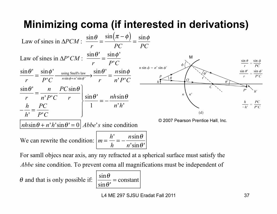
Minimizing coma (if interested in derivations)

Law of sines in ΔPCM : sinθr

=sin π −φ( )

PC= sinφ

PC

Law of sines in ΔP 'CM : sinθ 'r

= sinφ 'P 'C

sinθ 'r

= sinφ 'P 'C

using Snell's lawn sinφ=n ' sinφ '⎯ →⎯⎯⎯⎯ sinθ '

r= nsinφ

n ' P 'Csinθ '

r= n

n ' P 'CPC sinθ

r

− hh '

= PCP 'C

⎫

⎬⎪⎪

⎭⎪⎪

sinθ '1

= − nhsinθn 'h '

nhsinθ + n 'h 'sinθ ' = 0 Abbe 's sine condition

We can rewrite the condition: m = h 'h= − nsinθ

n 'sinθ 'For samll objecs near axis, any ray refracted at a spherical surface must satisfy the Abbe sine condition. To prevent coma all magnifications must be independent of

θ and that is only possible if: sinθsinθ '

= constant

M


Astigmatism and curvature of field

a Q( ) = 0C40r4 + 1C31h 'r3 cosθ

Aplanatic optics corrects spherical and coma

+ h '2 r 22C22 cos2θ

Astigmatism

+ 2C20

Curvature of field

⎛

⎝⎜⎜

⎞

⎠⎟⎟

+ 3C11h '3 r cosθAstigmatism and curvature of field have same dependencies to: a) off-axis distance of the object b) aperture of the system

Focal line for the tangential fan of rays tt’ In the sagittal plane

Elliptical image


Image of astigmatism

39


Amount of astigmatism for object point P = S-T

Principal rays From various object points

T to the left of S: Positive astigmatism

T to the right of S: negative astigmatism


If we use combination of lenses so that S and T image planes coinside on a single plane so called Petzval surface, we no longer have astigmatism but the image plane is now curved. This kind of aberration is called curvature of (image) field.

The sharp image forms on a curved surface.


For two thin lenses the Petzval surface is flat if n1 f1 + n2 f2 = 0This eliminates the curvature of the field as well.

For k thin lenses: 1ni fi

= 1RPi=1

k

∑

where Rp is the radius of Petzval surface.

We can also use apertures to flatten fieldslike in a simple box camera.For actual flattening the curvature of field we need 5th order analysis.


Chromatic aberration

Chromatic is not a Seidel aberration.It is caused by variation of refractive index with wavelength or dispersion.f , focal length of a lens depends on n and n depends on wavelength so f → f λ( )

Chromatic aberration for axial object points

Chromatic aberration for off-axial object points

Longitudinal

Transverse


Eliminating chromatic aberration

We can eleiminate chromatic aberration by using refractive elements of opposite power.Goal: finding the proper radii of curvature for an achromatic doublet.Fraunhofer spectral lines: λF = 486.1nm (hydrogen); λD = 587.6nm (sodium); λC = 656.3nm;Dispersive constant of a glass defined as:

V ≡ 1Δ=

nD −1nF − nC

where Δ is dispersive power.

Variations of n with λ is: ∂n∂λ

≅nF − nC

λF − λC


Eliminating chromatic aberration I

Power of the two lenses for the sodium yellow line:

P1D = 1f1D

= n1D −1( ) 1r11

− 1r12

⎛

⎝⎜⎞

⎠⎟= n1D −1( )K1

P2 D = 1f2 D

= n2 D −1( ) 1r21

− 1r22

⎛

⎝⎜⎞

⎠⎟= n2 D −1( )K2

Total power of two thin lenses with distance L between them:1f= 1

f1

+ 1f2

− Lf1 f2

→ P = P1 + P2 − LP1P2

Total power of two thin lenses cemented: P = P1 + P2 = n1 −1( )K1 + n2 −1( )K2


Eliminating chromatic aberration II

Power of two thin lenses cemented: P = n1 −1( )K1 + n2 −1( )K2

We want the power of the combined lens be independent of wavelength. To achieve that we set: ∂P / ∂λ( )D

= 0

∂P∂λ

= K1

∂n1

∂λ+ K2

∂n2

∂λ= 0 with ∂n

∂λ≅

nF − nC

λF − λC

K1

∂n1D

∂λ= K1

n1F − n1C

λF − λC

⎛

⎝⎜⎞

⎠⎟n1D −1n1D −1

⎛

⎝⎜⎞

⎠⎟=

P1D

λF − λC( )V1

;

K2

∂n2 D

∂λ= K2

n2 F − n2C

λF − λC

⎛

⎝⎜⎞

⎠⎟n2 D −1n2 D −1

⎛

⎝⎜⎞

⎠⎟=

P2 D

λF − λC( )V2

∂P∂λ

=P1D

λF − λC( )V1

+P2 D

λF − λC( )V2

= 0→V2P1D +V1P2 D = 0


Eliminating chromatic aberration

The powers of individual elements are:

V2 P1D +V1P2 D = 0P = P1D + P2 D

⎧⎨⎪

⎩⎪→

P1D = PD

−V1

V2 −V1

P2 D = PD

V2

V2 −V1

⎧

⎨⎪⎪

⎩⎪⎪

→

K1 =P1D

n1D −1= 1

r11

− 1r12

⎛

⎝⎜⎞

⎠⎟

K2 =P2 D

n2 D −1= 1

r21

− 1r22

⎛

⎝⎜⎞

⎠⎟

⎧

⎨

⎪⎪

⎩

⎪⎪

For simplicity we choose the crown glass to be equiconvex:

r12 = −r11

The curvature of the cemented surfaces has to match:

r21 = r12 and r22 =r12

1− K2r12

where K2 =1r21

− 1r22

⎛

⎝⎜⎞

⎠⎟


Correction of the chromatic aberrations


Achromats and apochromats


The use of a strong positive lens made from a low dispersion glass like crown coupled with a weaker high dispersion glass like flint an correct chromatic aberration for two colors. One could use three lenses to achieve the same focal length for three wavelengths. These are called apochromatic lenses.

Optical glasses


In a design process we take the indexes for the Fraunhofer lines from the manufacturer’s specification.

Documents

L4 Optical design Flow in-software and aberrations