Optical Design with Zemax - Institute of Applied Physics · 2012-10-13 · 5 13.11. Aberrations II Wave aberrations, Zernike polynomials, Point spread function, Optical transfer function

www.iap.uni-jena.de

Optical Design with Zemax

Lecture 2: Properties of optical systems I

2012-10-23

Herbert Gross

Winter term 2012

2 2 Properties of Optical Systems I

Preliminary time schedule

1 16.10. Introduction

Introduction, Zemax interface, menues, file handling, preferences, Editors, updates, windows,

Coordinate systems and notations, System description, Component reversal, system insertion,

scaling, 3D geometry, aperture, field, wavelength

2 23.10. Properties of optical systems I Diameters, stop and pupil, vignetting, Layouts, Materials, Glass catalogs, Raytrace, Ray fans

and sampling, Footprints

3 30.10. Properties of optical systems II Types of surfaces, Aspheres, Gratings and diffractive surfaces, Gradient media, Cardinal

elements, Lens properties, Imaging, magnification, paraxial approximation and modelling

4 06.11. Aberrations I Representation of geometrical aberrations, Spot diagram, Transverse aberration diagrams,

Aberration expansions, Primary aberrations,

5 13.11. Aberrations II Wave aberrations, Zernike polynomials, Point spread function, Optical transfer function

6 20.11. Optimization I Principles of nonlinear optimization, Optimization in optical design, Global optimization

methods, Solves and pickups, variables, Sensitivity of variables in optical systems

7 27.11. Optimization II Systematic methods and optimization process, Starting points, Optimization in Zemax

8 04.12 Imaging Fundamentals of Fourier optics, Physical optical image formation, Imaging in Zemax

9 11.12. Illumination Introduction in illumination, Simple photometry of optical systems, Non-sequential raytrace,

Illumination in Zemax

10 18.12. Advanced handling I

Telecentricity, infinity object distance and afocal image, Local/global coordinates, Add fold

mirror, Scale system, Make double pass, Vignetting, Diameter types, Ray aiming, Material

index fit

11 08.01. Advanced handling II Report graphics, Universal plot, Slider, Visual optimization, IO of data, Multiconfiguration,

Fiber coupling, Macro language, Lens catalogs

12 15.01. Correction I

Symmetry principle, Lens bending, Correcting spherical aberration, Coma, stop position,

Astigmatism, Field flattening, Chromatical correction, Retrofocus and telephoto setup, Design

method

13 22.01. Correction II Field lenses, Stop position influence, Aspheres and higher orders, Principles of glass

selection, Sensitivity of a system correction, Microscopic objective lens, Zoom system

14 29.01. Physical optical modelling I Gaussian beams, POP propagation, polarization raytrace, polarization transmission,

polarization aberrations

15 05.02. Physical optical modelling II coatings, representations, transmission and phase effects, ghost imaging, general straylight

with BRDF

1. Diameters

2. Stops and Pupil definition

3. Vignetting

4. Layout

5. Materials and glass catalogs

6. Raytrace

7. Ray fans and sampling

8. Footprints


Contents 2nd Lecture

Pupil stop defines:

1. chief ray angle w

2. aperture cone angle u

The chief ray gives the center line of the oblique ray cone of an off-axis object point

The coma rays limit the off-axis ray cone

The marginal rays limit the axial ray cone

y

y'

stop

pupil

coma ray

chief ray

marginal ray

aperture

angle

u

field anglew

object

image

2 Properties of Optical Systems I

Optical system stop

The physical stop defines

the aperture cone angle u

The real system may be complex

The entrance pupil fixes the

acceptance cone in the

object space

The exit pupil fixes the

acceptance cone in the

image space

uobject

image

stop

EnP

ExP

object

image

black box

details complicated

real

system

? ?

Ref: Julie Bentley


Optical system stop

Relevance of the system pupil :

Brightness of the image

Transfer of energy

Resolution of details

Information transfer

Image quality

Aberrations due to aperture

Image perspective

Perception of depth

Compound systems:

matching of pupils is necessary, location and size


Properties of the pupil

exit

pupil

upper

marginal ray

chief

ray

lower coma

raystop

field point

of image

UU'

W

lower marginal

ray

upper coma

ray

on axis

point of

image

outer field

point of

object

object

point

on axis

entrance

pupil


Entrance and exit pupil

Generalization of paraxial picture:

Principal surface works as effective location of ray bending

Paraxial approximation: plane

Real systems with corrected

sine-condition (aplanatic):

principal sphere

effektive surface of

ray bending P'

y

f'

U'

P


Pupil sphere

Pupil sphere:

equidistant sine-

sampling

z

object entrance

pupil

image

yo y'

U U'sin(U) sin(U')

exit

pupil

objectyo

equidistant

sin(U)

angle U non-

equidistant

pupil

sphere


Pupil sphere

Different possible options for specification of the aperture in Zemax:

1. Entrance pupil diameter

2. Image space F#

3. Object space NA

4. Paraxial working F#

5. Object cone angle

6. Floating by stop size

Stop location:

1. Fixes the chief ray intersection point

2. input not necessary for telecentric object space

3. is used for aperture determination in case of aiming

Special cases:

1. Object in infinity (NA, cone angle input impossible)

2. Image in infinity (afocal)

3. Object space telecentric


Aperture data in Zemax

3D-effects due to vignetting

Truncation of the at different surfaces for the upper and the lower part

of the cone

2 Properties of optical systems I

Vignetting

object lens 1 lens 2 imageaperture

stop

lower

truncation

upper

truncation

sagittal

trauncation

chief

ray

coma

rays

Truncation of the light cone

with asymmetric ray path

for off-axis field points

Intensity decrease towards

the edge of the image

Definition of the chief ray:

ray through energetic centroid

Vignetting can be used to avoid

uncorrectable coma aberrations

in the outer field

Effective free area with extrem

aspect ratio:

anamorphic resolution

projection of the

rim of the 2nd lens

projection of the

rim of the 1st lens

Projektion der

Aperturblende

free area of the

aperture

sagittal

coma rays

meridional

coma rayschief

ray

2 Properties of optical systems I

Vignetting

1. Determination of one surface as system stop:

- Fixes the chief ray intersection point with axis

- can be set in surface properties menu

- indicated by STO in lens data editor

- determines the aperture for the option 'float by stop size'

2. Diameters in lens data editor

- indicated U for user defined

- only circular shape

- effects drawing

- effects ray vignetting

- can be used to draw 'nice lenses' with

overflow of diameter

3. Diameters as surface properties:

- effects on rays in drawing (vignetting)

- no effect on lens shapes in drawing

- also complicated shapes and decenter

possible

- indicated in lens data editor by a star


Diameters and stop sizes

4. Individual aperture sizes for every field point can be set by the vignetting factors of the

Field menu

- real diameters at surfaces must be set

- reduces light cones are drawn in the layout


Diameters and stop sizes

Graphical control of system

and ray path

Principal options in Zemax:

1. 2D section for circular symmetry

2. 3D general drawing

Several options in settings

Zooming with mouse


Layout options

Different options for 3D case

Multiconfiguration plot possible

Rayfan can be chosen


Layout options

Professional graphic

Many layout options

Rotation with mouse or arrow buttons


Layout options

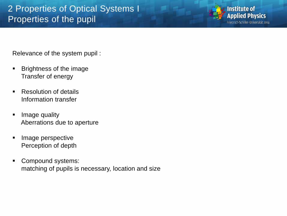
Important types of optical materials:

1. Glasses

2. Crystals

3. Liquids

4. Plastics, cement

5. Gases

6. Metals

Optical parameters for characterization of materials

1. Refractive index, spectral resolved n(l)

2. Spectral transmission T(l)

3. Reflectivity R

4. Absorption

5. Anisotropy, index gradient, eigenfluorescence,…

Important non-optical parameters

1. Thermal expansion coefficient

2. Hardness

3. Chemical properties (resistence,…)


Optical materials

l in [nm] Name Color Element

248.3 UV Hg

280.4 UV Hg

296.7278 UV Hg

312.5663 UV Hg

334.1478 UV Hg

365.0146 i UV Hg

404.6561 h violett Hg

435.8343 g blau Hg

479.9914 F' blau Cd

486.1327 F blau H

546.0740 e grün Hg

587.5618 d gelb He

589.2938 D gelb Na

632.8 HeNe-Laser

643.8469 C' rot Cd

656.2725 C rot H

706.5188 r rot He

852.11 s IR Cä

1013.98 t IR Hg

1060.0 Nd:YAG-Laser


Test wavelengths

refractive

index n

1.65

1.6

1.5

1.8

1.55

1.75

1.7

BK7

SF1

l0.5 0.75 1.0 1.25 1.751.5 2.0

1.45

Flint

Kron

Description of dispersion:

Abbe number

Visual range of wavelengths:

Typical range of glasses

ne = 20 ...120

Two fundamental types of glass:

Crone glasses:

n small, n large

Flint glasses

n large, n small

n ll

n

n nF C

1

' '

ne

e

F C

n

n n

1

' '


Dispersion and Abbe number

Material with different dispersion values:

- Different curvature of the dispersion curve

- Stronger change of index over wavelength for large dispersion

- Inversion of index sequence at the boundaries of the spectrum possible

refractive index n

F6

SK18A

l

1.675

1.7

1.65

1.625

1.60.5 0.75 1.0 1.25 1.751.5 2.0


Dispersion

Schott formula

empirical

Sellmeier

Based on oscillator model

Bausch-Lomb

empirical

Herzberger


Hartmann


n a a a a a ao

1

2

2

2

3

4

4

6

5

8l l l l l

n A B C( )ll

l l

l

l l

2

212

2

222

n A B CD E

Fo

o

( )

( )

l l ll

l

l ll

l l

2 4

2

2

2 22

2 2

mmit

aaaan

o

oo

o

l

llllll

168.0

)(222

3

22

22

1

lll

5

4

3

1)(a

a

a

aan o


Dispersion formulas

Relative partial dispersion :

Change of dispersion slope with l

Definition of local slope for selected

wavelengths relative to secondary

colors

Special selections for characteristic

ranges of the visible spectrum

l = 656 / 1014 nm far IR

l = 656 / 852 nm near IR

l = 486 / 546 nm blue edge of VIS

l = 435 / 486 nm near UV

l = 365 / 435 nm far UV

P

n n

n nF C

l l

l l1 2

1 2

' '

l

n

400 600 800 1000700500 900 1100

e : 546 nm

main color

F' : 480 nm

1. secondary

color

g : 435 nmUV edge

C' : 644 nm

s : 852 nm

IR edge

t : 1014 nm

IR edge

C : 656 nmF : 486 nm

d : 588 nm

i : 365 nm

UV edge

i - g

F - C

C - s

C - t

F - e

g - F

2. secondary

color

1.48

1.49

1.5

1.51

1.52

1.53

1.54

n(l)


Relative partial dispersion

Usual representation of

glasses:

diagram of refractive index

vs dispersion n(n)

Left to right:

Increasing dispersion

decreasing Abbe number


Glass diagram

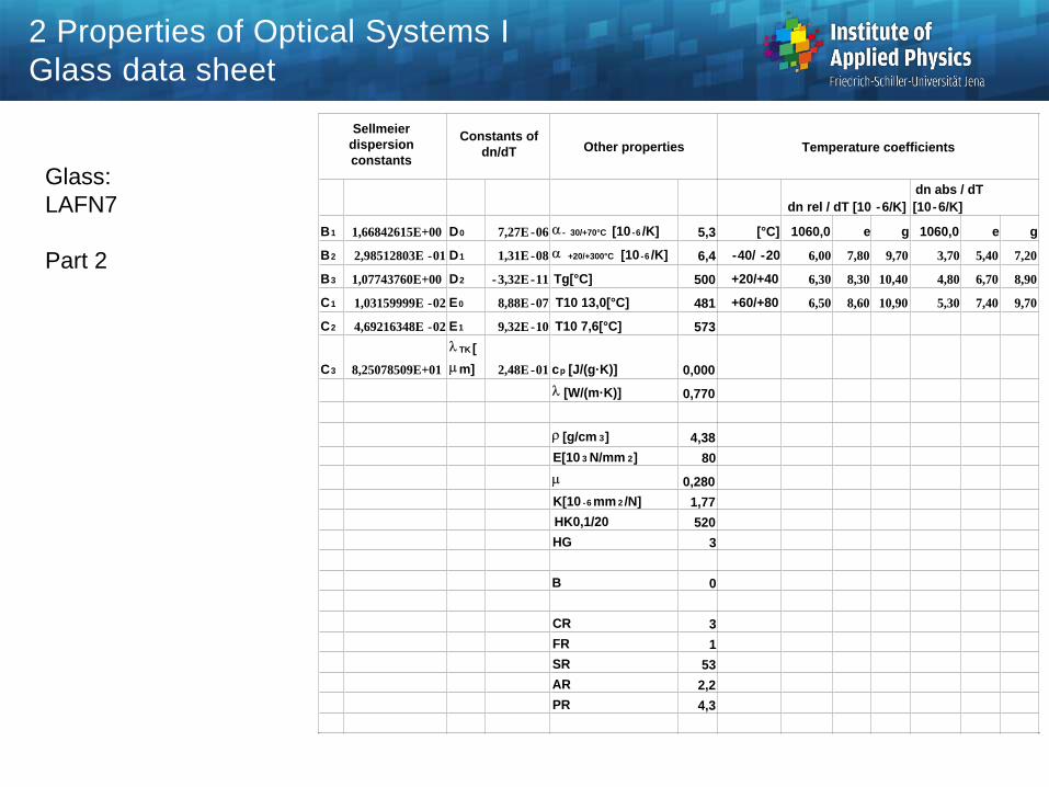
Glass:

LAFN7

Part 1

Main data Refractive

indices

Internal transmission

data

relative partial

dispersion

Anomalous

partial

dispersion

l

[nm] n

l

[nm]

i [10

mm]

i [25

mm]

LAFN7 750350.4

38 n2325,4 2325,4 1,70211 2500,0 0,380 0,090 Ps,t 0,2360 Pc,t 0,0174

nd 1,74950 n1970,1 1970,1 1,70934 2325,4 0,700 0,410 PC,s 0,4921 Pc,s 0,0078

ne 1,75458 n1529,6 1529,6 1,71726 1970,1 0,940 0,850 Pd,C 0,2941 PF,e - 0,0011

nd 34,95 n1060,0 1060,0 1,72642 1529,6 0,984 0,960 Pe,d 0,2369 Pg,F - 0,0025

ne 34,72 nt 1014,0 1,72758 1060,0 0,998 0,996 Pg,F 0,5825 Pi,g - 0,0093

nF-nC 0,02145 ns 852,1 1,73264 700,0 0,998 0,996 Pi,h 0,9160

nF'-nC' 0,021735 nr 706,5 1,73970 660,0 0,998 0,995

nC 656,3 1,74319 620,0 0,998 0,995 P's,t 0,2329

nC' 643,8 1,74418 580,0 0,998 0,995 P'C',s 0,5311

n632,8 632,8 1,74511 546,1 0,998 0,994 P'd,C' 0,2446

nD 589,3 1,74931 500,0 0,998 0,994 P'e,d 0,2338

nd 587,6 1,74950 460,0 0,993 0,982 P'g,F' 0,5158

ne 546,1 1,75458 435,8 0,986 0,965 P'i,h 0,9037

nF 486,1 1,76464 420,0 0,976 0,940

nF' 480,0 1,76592 404,7 0,950 0,880

ng 435,8 1,77713 400,0 0,940 0,850

nh 404,7 1,78798 390,0 0,910 0,780

ni 365,0 1,80762 380,0 0,840 0,650

n3 34,1 334,1 0,00000 370,0 0,690 0,400

n312,6 312,6 0,00000 365,0 0,550 0,220

n296,7 296,7 0,00000 350,0 0,130 0,010

n280,4 280,4 0,00000 334,1 0,000 0,000

n248,3 248,3 0,00000 320,0 0,000 0,000

310,0 0,000 0,000


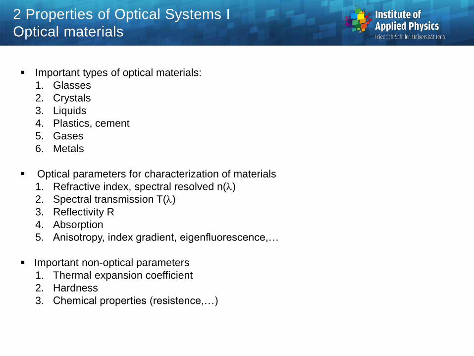
Glass data sheet

Sellmeier

dispersion

constants

Constants of

dn/dT

Other properties Temperature coefficients

dn rel / dT [10 -6/K]

dn abs / dT

[10-6/K]

B1 1,66842615E+00 D0 7,27E -06 - 30/+70°C [10 -6 /K] 5,3 [°C] 1060,0 e g 1060,0 e g

B2 2,98512803E -01 D1 1,31E -08 +20/+300°C [10 -6 /K] 6,4 -40/ -20 6,00 7,80 9,70 3,70 5,40 7,20

B3 1,07743760E+00 D2 - 3,32E -11 Tg[°C] 500 +20/+40 6,30 8,30 10,40 4,80 6,70 8,90

C1 1,03159999E -02 E0 8,88E -07 T10 13,0[°C] 481 +60/+80 6,50 8,60 10,90 5,30 7,40 9,70

C2 4,69216348E -02 E1 9,32E -10 T10 7,6[°C] 573

C3 8,25078509E+01

l TK [

m] 2,48E -01 cp [J/(g·K)] 0,000

l [W/(m·K)] 0,770

[g/cm 3] 4,38

E[10 3 N/mm 2] 80

0,280

K[10 -6 mm 2 /N] 1,77

HK0,1/20 520

HG 3

B 0

CR 3

FR 1

SR 53

AR 2,2

PR 4,3

Glass:

LAFN7

Part 2


Glass data sheet

Crown glasses

n

n

e e

e e

für n

für n

54 7 16028

49 7 16028

. .

. .

Flint glasses

n

n

e e

e e

für n

für n

54 7 16028

49 7 16028

. .

. .

n

n

80 70 60 50 40 30 2025354555657585

1.45

1.50

1.55

1.60

1.65

1.70

1.75

1.80

1.85

1.90

1.95

2.00

LaK

LaSF

SF

TiSF

TiF

BaSF

F

LFLLF

BaLF

LaF

PSK

PK

FK TiK

BKK

SK

BaK

SSK

KF

crown

glass

flint

glass

BaF


Ranges of glass map

n

n

20 30 40 50 60 70 80 90 1001.4

1.5

1.6

1.7

1.8

1.9

2

20 30 40 50 60 70 80 90 1001.4

1.5

1.6

1.7

1.8

1.9

2

Schott Ohara

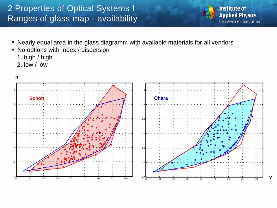
Nearly equal area in the glass diagramm with available materials for all vendors

No options with Index / dispersion

1. high / high

2. low / low


Ranges of glass map - availability

zoptical

axis

y j

u'j-1

ij

dj-1

ds j-1

ds j

i'j

u'j

n j

nj-1

mediummedium

surface j-1

surface j

ray

dj

vertex distance

oblique thickness

rr

Ray: straight line between two intersection points

System: sequence of spherical surfaces

Data: - radii, curvature c=1/r

- vertex distances

- refractive indices

- transverse diameter

Surfaces of 2nd order:

Calculation of intersection points

analytically possible: fast

computation


Scheme of raytrace

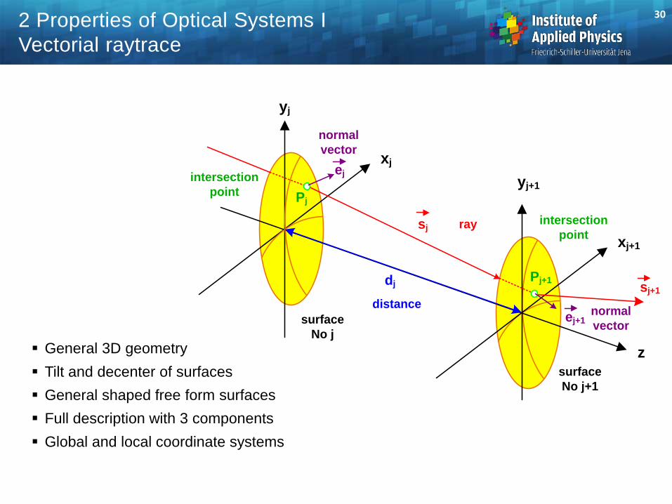
yj

z

Pj+1

sj

xj

yj+1

xj+1

Pj

surface

No j

surface

No j+1

dj sj+1

intersection

point

ej

normal

vector

ej+1

ray

distance

intersection

point

normal

vector

General 3D geometry

Tilt and decenter of surfaces

General shaped free form surfaces

Full description with 3 components

Global and local coordinate systems


Vectorial raytrace

r D R F R D rH H V V'

Single surface:

- tilt and decenter before refraction

- decenter and tilt after refraction

General setup for position and orientation in 3D

z

x

y

z

xF

yF

zF

j-1

j+1global

coordinates

surface

No j

VV

VH

KV

KH

shift before

shift after

tilt after

tilt before


Surfaces in 3D

Restrictions:

- surfaces of second order, fast analytical calculation of intersection point possible

- homogeneous media

Direction unit vector of the straight ray

Vector of intersection point on a surface

Ray equation with skew thickness dsj

index j of the surface and the space behind

Equation of the surface 2.order

The coefficients H, F, G contains the surface shape parameters

s j

j

j

j

r

x

y

z

j

j

j

j

11,1 jjsjj sdrr

02 1,

2

1, jjsjjsj GdFdH


Vectorial raytrace formulas

Special case spherical surface with

curvature c = 1/R

Coefficients H, G, F

Unit vector normal to the surface

Insertion of the ray equation into surface equation:

skew thickness

Angle of incidence

Refraction

or

reflection

jj cH

jjjjjj zzyxcG 2222

jjjjjjjjj zyxcF

jj

jj

jj

j

zc

yc

xc

e

1

jjjj

j

js

GHFF

Gd

21,

cosi s ej j j

cos ' cosin

nij

j

j

j

1 11

2

2

cos ' cosi ij j



Auxiliary parameter

New ray direction vector

j j j j jn i n i 1 cos ' cos

s

n

ns

nej

j

j

j

j

j

j

1

1 1



Vignetting/truncation of ray at finite sized diameter:

can or can not considered (optional)

No physical intersection point of ray with surface

Total internal reflection

Negative edge thickness of lenses

Negative thickness without mirror-reflection

Diffraction at boundaries

index

j

index

j+1

axis

negative

un-physical

regular

irregular

axis

no intersection

point

axis

intersection:

- mathematical possible

- physical not realized

axis

total

internal

reflection


Raytrace errors

Meridional rays:

in main cross section plane

Sagittal rays:

perpendicular to main cross

section plane

Coma rays:

Going through field point

and edge of pupil

Oblique rays:

without symmetry

axis

y

x

p

p

pupil plane

object plane

x

y

axissagittal ray

meridional

marginal ray

skew raychief ray

sagittal coma

ray

upper

meridional

coma ray

lower

meridional

coma ray

field

point

axis point


Special rays in 3D

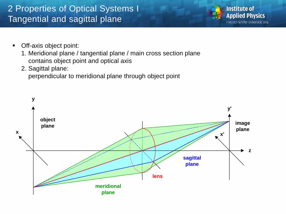
Off-axis object point:

1. Meridional plane / tangential plane / main cross section plane

contains object point and optical axis

2. Sagittal plane:

perpendicular to meridional plane through object point

x

y

x'

y'

z

lens

meridional

plane

sagittal

plane

object

planeimage

plane


Tangential and sagittal plane

Ray fan:

2-dimensional plane set of rays

Ray cone:

3-dimensional filled ray cone

object

point

pupil

grid


Ray fans and ray cones

Transverse aberrations:

Ray deviation form ideal image point in meridional and sagittal plane respectively

The sampling of the pupil is only filled in two perpendicular directions along the axes

No information on the performance of rays in the quadrants of the pupil

x

y

pupil

tangential

ray fan

sagittal

ray fanobject

point


Ray fan selection for transverse aberrations plots

Pupil sampling for calculation of transverse aberrations:

all rays from one object point to all pupil points on x- and y-axis

Two planes with 1-dimensional ray fans

No complete information: no skew rays

y'p

x'p

yp

xp x'

y'

z

yo

xo

object

plane

entrance

pupil

exit

pupil

image

plane

tangential

sagittal


Pupil sampling

Pupil sampling in 3D for spot diagram:

all rays from one object point through all pupil points in 2D

Light cone completly filled with rays

y'p

x'p

yp

xp x'

y'

z

yo

xo

object

plane

entrance

pupil

exit

pupil

image

plane


Sampling of pupil area

Different types of sampling with pro and con‘s:

1. Polar grid: not isoenergetic

2. Cartesian: good for FFT, boundary discretization bad

3. Isoenergetic circular: good

4. Hexagonal: good

5. Statistical: good non-regularity,

holes ?

polar grid cartesian isoenergetic circular

hexagonal statistical


Pupil sampling

Artefacts due to regular gridding of the pupil of the spot in the image plane

In reality a smooth density of the spot is true

The line structures are discretization effects of the sampling

hexagonal statisticalcartesian


Artefacts of pupil sampling

Looking for the ray bundle cross sections


Footprints

Documents

Optical Design with Zemax - Institute of Applied Physics · 2012-10-13 · 5 13.11. Aberrations II Wave aberrations, Zernike polynomials, Point spread function, Optical transfer function