1

Lab 1: Getting familiar with LabVIEW: Part I

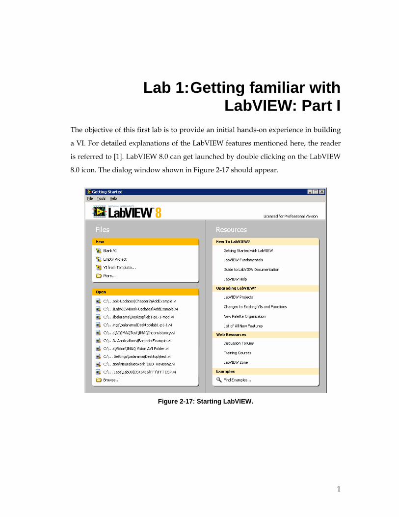
The objective of this first lab is to provide an initial hands-on experience in building

a VI. For detailed explanations of the LabVIEW features mentioned here, the reader

is referred to [1]. LabVIEW 8.0 can get launched by double clicking on the LabVIEW

8.0 icon. The dialog window shown in Figure 2-17 should appear.

Figure 2-17: Starting LabVIEW.

2

L1.1 Building a Simple VI

To become familiar with the LabVIEW programming environment, it is found to be

more effective if one goes through a simple example. The example presented here

consists of calculating the sum and average of two input values. This example is

described in a step-by-step fashion below.

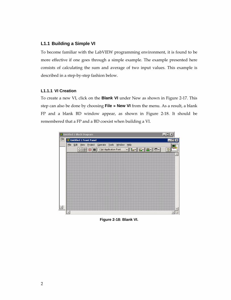
L1.1.1 VI Creation To create a new VI, click on the Blank VI under New as shown in Figure 2-17. This

step can also be done by choosing File » New VI from the menu. As a result, a blank

FP and a blank BD window appear, as shown in Figure 2-18. It should be

remembered that a FP and a BD coexist when building a VI.

Figure 2-18: Blank VI.

3

Clearly, the number of inputs and outputs to a VI is dependent on its

function. In this example, two inputs and two outputs are needed, one output

generating the sum and the other the average of two input values. The inputs are

created by locating two Numeric Controls on the FP. This is done by right-

clicking on an open area of the FP to bring up the Controls palette, followed by

choosing Controls » Modern » Numeric » Numeric Control. Each numeric control

automatically places a corresponding terminal icon on the BD. Double clicking on a

numeric control highlights its counterpart on the BD, and vice versa.

Next, let us label the two inputs as x and y. This is achieved by using the

Labeling tool from the Tools palette, which can be displayed by choosing View »

Tools Palette from the menu bar. Choose the Labeling tool and click on the default

labels, Numeric and Numeric 2, in order to edit them. Alternatively, if the

automatic tool selection mode is enabled by clicking Automatic Tool Selection in

the Tools palette, the labels can be edited by simply double clicking on the default

labels. Editing a label on the FP changes its corresponding terminal icon label on the

BD, and vice versa.

Similarly, the outputs are created by locating two Numeric Indicators

(Controls » Modern » Numeric » Numeric Indicator) on the FP. Each numeric

indicator automatically places a corresponding terminal icon on the BD. Edit the

labels of the indicators to read Sum and Average.

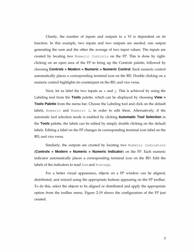
For a better visual appearance, objects on a FP window can be aligned,

distributed, and resized using the appropriate buttons appearing on the FP toolbar.

To do this, select the objects to be aligned or distributed and apply the appropriate

option from the toolbar menu. Figure 2-19 shows the configuration of the FP just

created.

4

Figure 2-19: FP configuration.

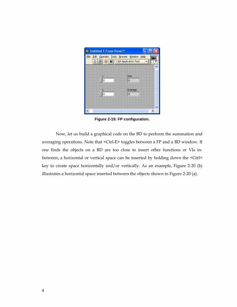
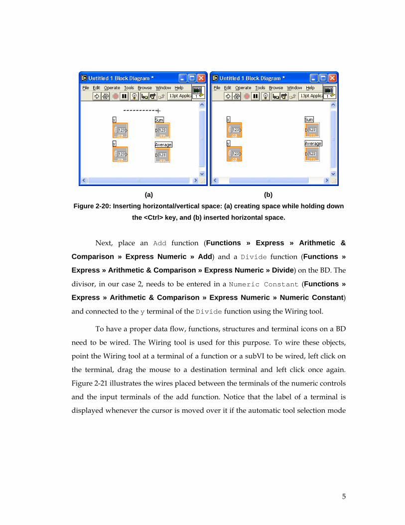
Now, let us build a graphical code on the BD to perform the summation and

averaging operations. Note that <Ctrl-E> toggles between a FP and a BD window. If

one finds the objects on a BD are too close to insert other functions or VIs in-

between, a horizontal or vertical space can be inserted by holding down the <Ctrl>

key to create space horizontally and/or vertically. As an example, Figure 2-20 (b)

illustrates a horizontal space inserted between the objects shown in Figure 2-20 (a).

5

(a) (b)

Figure 2-20: Inserting horizontal/vertical space: (a) creating space while holding down the <Ctrl> key, and (b) inserted horizontal space.

Next, place an Add function (Functions » Express » Arithmetic &

Comparison » Express Numeric » Add) and a Divide function (Functions »

Express » Arithmetic & Comparison » Express Numeric » Divide) on the BD. The

divisor, in our case 2, needs to be entered in a Numeric Constant (Functions »

Express » Arithmetic & Comparison » Express Numeric » Numeric Constant)

and connected to the y terminal of the Divide function using the Wiring tool.

To have a proper data flow, functions, structures and terminal icons on a BD

need to be wired. The Wiring tool is used for this purpose. To wire these objects,

point the Wiring tool at a terminal of a function or a subVI to be wired, left click on

the terminal, drag the mouse to a destination terminal and left click once again.

Figure 2-21 illustrates the wires placed between the terminals of the numeric controls

and the input terminals of the add function. Notice that the label of a terminal is

displayed whenever the cursor is moved over it if the automatic tool selection mode

6

is enabled. Also, note that the Run button on the toolbar remains broken until

the wiring process is completed.

Figure 2-21: Wiring BD objects.

For better readability of a BD, wires which are hidden behind objects or

crossed over other wires can be cleaned up by right-clicking on them and choosing

Clean Up Wire from the shortcut menu. Any broken wires can be cleared by

pressing <Ctrl-B> or Edit » Remove Broken Wires.

The label of a BD object, such as a function, can be shown (or hidden) by

right-clicking on the object and checking (or unchecking) Visible Items » Label from

the shortcut menu. Also, a terminal icon corresponding to a numeric control or

indicator can be shown as a data type terminal icon. This is done by right-clicking on

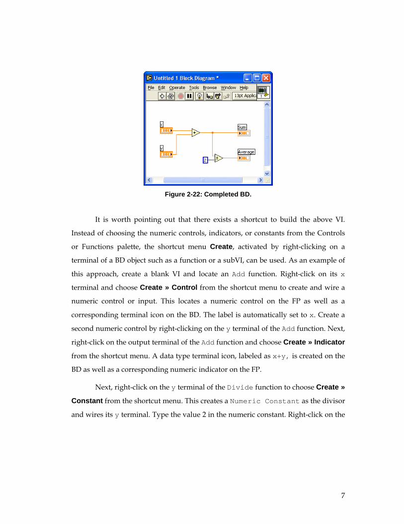
the terminal icon and unchecking View As Icon from the shortcut menu. Figure 2-22

shows an example where the numeric controls and indicators are shown as data type

terminal icons. The notation DBL represents double precision data type.

7

Figure 2-22: Completed BD.

It is worth pointing out that there exists a shortcut to build the above VI.

Instead of choosing the numeric controls, indicators, or constants from the Controls

or Functions palette, the shortcut menu Create, activated by right-clicking on a

terminal of a BD object such as a function or a subVI, can be used. As an example of

this approach, create a blank VI and locate an Add function. Right-click on its x

terminal and choose Create » Control from the shortcut menu to create and wire a

numeric control or input. This locates a numeric control on the FP as well as a

corresponding terminal icon on the BD. The label is automatically set to x. Create a

second numeric control by right-clicking on the y terminal of the Add function. Next,

right-click on the output terminal of the Add function and choose Create » Indicator

from the shortcut menu. A data type terminal icon, labeled as x+y, is created on the

BD as well as a corresponding numeric indicator on the FP.

Next, right-click on the y terminal of the Divide function to choose Create »

Constant from the shortcut menu. This creates a Numeric Constant as the divisor

and wires its y terminal. Type the value 2 in the numeric constant. Right-click on the

8

output terminal of the Divide function, labeled as x/y, and choose Create »

Indicator from the shortcut menu. In case a wrong option is chosen, the terminal

does not get wired. A wrong terminal option can be easily changed by right-clicking

on the terminal and choosing Change to Control or Change to Constant from the

shortcut menu.

To save the created VI for later use, choose File » Save from the menu or

press <Ctrl-S> to bring up a dialog window to enter a name. Type Sum and

Average as the VI name and click Save.

To test the functionality of the VI, enter some sample values in the numeric

controls on the FP and run the VI by choosing Operate » Run, by pressing <Ctrl-R>,

or by clicking the Run button on the toolbar. From the displayed output values in the

numeric indicators, the functionality of the VI can be verified. Figure 2-23 illustrates

the outcome after running the VI with two inputs 10 and 30.

Figure 2-23: VI verification.

9

L1.1.2 SubVI Creation If a VI is to be used as part of a higher level VI, its connector pane needs to be

configured. A connector pane assigns inputs and outputs of a subVI to its terminals

through which data are exchanged. A connector pane can be displayed by right-

clicking on the top right corner icon of a FP and selecting Show Connector from the

shortcut menu.

The default pattern of a connector pane is determined based on the number

of controls and indicators. In general, the terminals on the left side of a connector

pane pattern are used for inputs, and the ones on the right side for outputs.

Terminals can be added to or removed from a connector pane by right-clicking and

choosing Add Terminal or Remove Terminal from the shortcut menu. If a change is

to be made to the number of inputs/outputs or to the distribution of terminals, a

connector pane pattern can be replaced with a new one by right-clicking and

choosing Patterns from the shortcut menu. Once a pattern is selected, each terminal

needs to be reassigned to a control or an indicator by using the Wiring tool, or by

enabling the automatic tool selection mode.

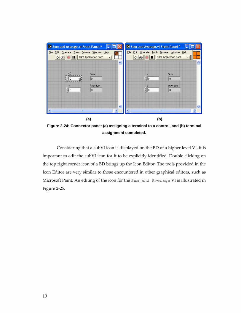
Figure 2-24 (a) illustrates assigning a terminal of the Sum and Average VI

to a numeric control. The completed connector pane is shown in Figure 2-24 (b).

Notice that the output terminals have thicker borders. The color of a terminal reflects

its data type.

10

(a) (b)

Figure 2-24: Connector pane: (a) assigning a terminal to a control, and (b) terminal assignment completed.

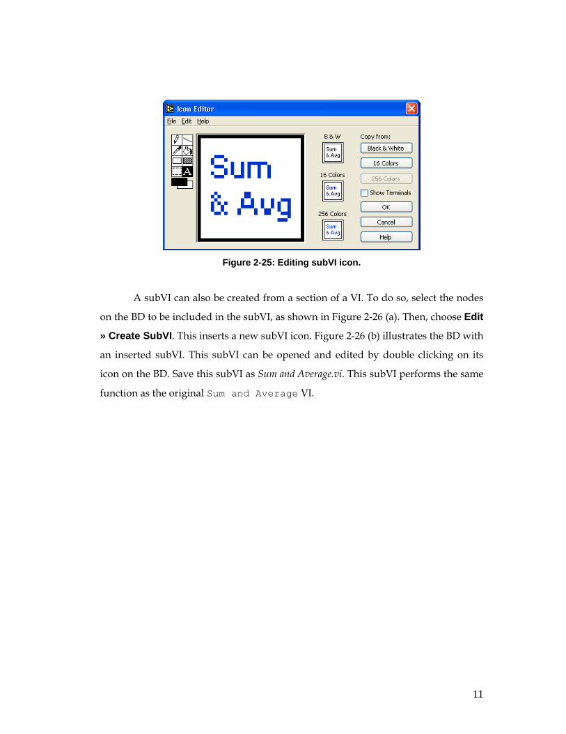
Considering that a subVI icon is displayed on the BD of a higher level VI, it is

important to edit the subVI icon for it to be explicitly identified. Double clicking on

the top right corner icon of a BD brings up the Icon Editor. The tools provided in the

Icon Editor are very similar to those encountered in other graphical editors, such as

Microsoft Paint. An editing of the icon for the Sum and Average VI is illustrated in

Figure 2-25.

11

Figure 2-25: Editing subVI icon.

A subVI can also be created from a section of a VI. To do so, select the nodes

on the BD to be included in the subVI, as shown in Figure 2-26 (a). Then, choose Edit

» Create SubVI. This inserts a new subVI icon. Figure 2-26 (b) illustrates the BD with

an inserted subVI. This subVI can be opened and edited by double clicking on its

icon on the BD. Save this subVI as Sum and Average.vi. This subVI performs the same

function as the original Sum and Average VI.

12

(a) (b)

Figure 2-26: Creating a subVI: (a) selecting nodes to make a subVI, and (b) inserted subVI icon.

In Figure 2-27, the completed FP and BD of the Sum and Average VI are

shown.

Figure 2-27: Sum and Average VI.

13

L1.2 Using Structures and SubVIs

Let us now consider another example to demonstrate the use of structures and

subVIs. In this example, a VI is used to show the sum and average of two input

values in a continuous fashion. The two inputs can be altered by the user. If the

average of the two inputs becomes greater than a preset threshold value, a LED

warning light is lit.

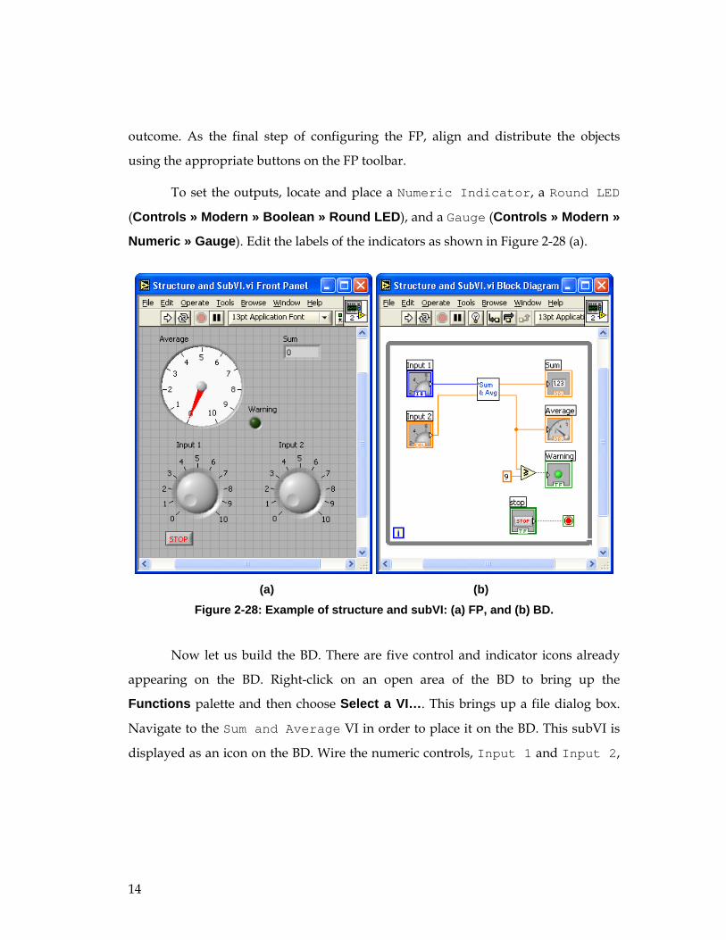
As the first step to build such a VI, build a FP as shown in Figure 2-28 (a). For

the inputs, consider two Knobs (Controls » Modern » Numeric » Knob). Adjust the

size of the knobs by using the Positioning tool. Properties of knobs such as precision

and data type can be modified by right-clicking and choosing Properties from the

shortcut menu. A Knob Properties dialog box is brought up and an Appearance tab

is shown by default. Edit the label of one of the knobs to read Input 1. Select the

Data Range tab, and click Representation to change the data type from double

precision to byte by selecting Byte among the displayed data types. This can also be

achieved by right-clicking on the knob and choosing Representation » Byte from

the shortcut menu. In the Data Range tab, a default value needs to be specified. In

this example, the default value is considered to be 0. The default value can be set by

right-clicking on the control and choosing Data Operations » Make Current Value

Default from the shortcut menu. Also, this control can be set to a default value by

right-clicking and choosing Data Operations » Reinitialize to Default Value from

the shortcut menu.

Label the second knob as Input 2 and repeat all the adjustments as done for

the first knob except for the data representation part. The data type of the second

knob is specified to be double precision in order to demonstrate the difference in the

14

outcome. As the final step of configuring the FP, align and distribute the objects

using the appropriate buttons on the FP toolbar.

To set the outputs, locate and place a Numeric Indicator, a Round LED

(Controls » Modern » Boolean » Round LED), and a Gauge (Controls » Modern »

Numeric » Gauge). Edit the labels of the indicators as shown in Figure 2-28 (a).

(a) (b)

Figure 2-28: Example of structure and subVI: (a) FP, and (b) BD.

Now let us build the BD. There are five control and indicator icons already

appearing on the BD. Right-click on an open area of the BD to bring up the

Functions palette and then choose Select a VI…. This brings up a file dialog box.

Navigate to the Sum and Average VI in order to place it on the BD. This subVI is

displayed as an icon on the BD. Wire the numeric controls, Input 1 and Input 2,

15

to the x and y terminals, respectively. Also, wire the Sum terminal of the subVI to the

numeric indicator labeled Sum, and the Average terminal to the gauge indicator

labeled Average.

A Greater or Equal? function is located from Functions »

Programming » Comparison » Greater or Equal? in order to compare the average

output of the subVI with a threshold value. Create a wire branch on the wire

between the Average terminal of the subVI and its indicator via the Wiring tool.

Then, extend this wire to the x terminal of the Greater or Equal? function.

Right-click on the y terminal of the Greater or Equal? function and choose

Create » Constant in order to place a Numeric Constant. Enter 9 in the numeric

constant. Then, wire the Round LED, labeled as Warning, to the x>=y? terminal of

this function to provide a Boolean value.

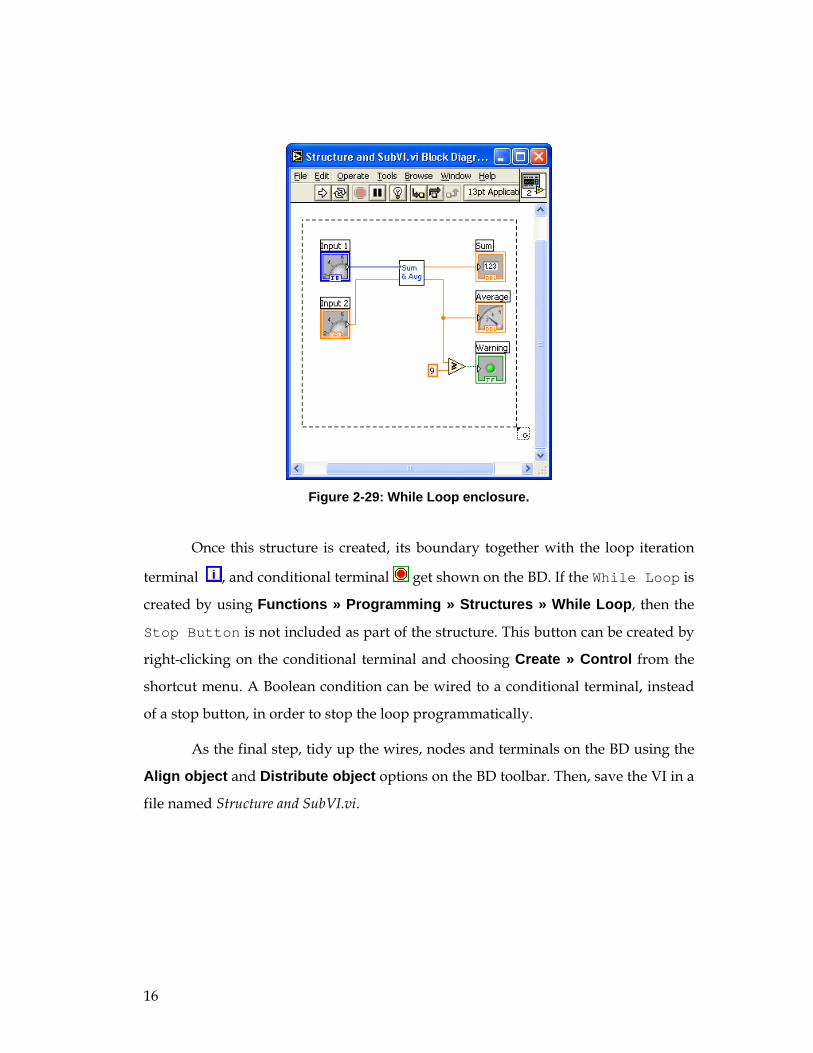
In order to run the VI continuously, a While Loop structure is used. Choose

Functions » Programming » Structures » While Loop to create a While Loop.

Change the size by dragging the mouse to enclose the objects in the While Loop as

illustrated in Figure 2-29.

16

Figure 2-29: While Loop enclosure.

Once this structure is created, its boundary together with the loop iteration

terminal , and conditional terminal get shown on the BD. If the While Loop is

created by using Functions » Programming » Structures » While Loop, then the

Stop Button is not included as part of the structure. This button can be created by

right-clicking on the conditional terminal and choosing Create » Control from the

shortcut menu. A Boolean condition can be wired to a conditional terminal, instead

of a stop button, in order to stop the loop programmatically.

As the final step, tidy up the wires, nodes and terminals on the BD using the

Align object and Distribute object options on the BD toolbar. Then, save the VI in a

file named Structure and SubVI.vi.

17

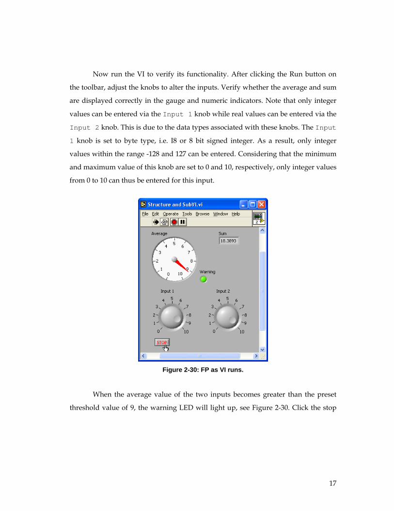
Now run the VI to verify its functionality. After clicking the Run button on

the toolbar, adjust the knobs to alter the inputs. Verify whether the average and sum

are displayed correctly in the gauge and numeric indicators. Note that only integer

values can be entered via the Input 1 knob while real values can be entered via the

Input 2 knob. This is due to the data types associated with these knobs. The Input

1 knob is set to byte type, i.e. I8 or 8 bit signed integer. As a result, only integer

values within the range -128 and 127 can be entered. Considering that the minimum

and maximum value of this knob are set to 0 and 10, respectively, only integer values

from 0 to 10 can thus be entered for this input.

Figure 2-30: FP as VI runs.

When the average value of the two inputs becomes greater than the preset

threshold value of 9, the warning LED will light up, see Figure 2-30. Click the stop

18

button on the FP to stop the VI. Otherwise, the VI keeps running until the

conditional terminal of the While Loop becomes true.

L1.3 Create an Array with Indexing

Auto-indexing enables one to read/write each element from/to a data array in a

loop structure. In this section, this feature is covered.

Let us first locate a For Loop (Functions » Programming » Structures »

For Loop). Right-click on its count terminal and choose Create » Constant from the

shortcut menu to set the number of iterations. Enter 10 so that the code inside it gets

repeated 10 times. Note that the current loop iteration count, which is read from the

iteration terminal, starts at index 0 and ends at index 9.

Place a Random Number (0-1) function (Functions » Programming »

Numeric » Random Number (0-1)) inside the For Loop and wire the output

terminal of this function, number (0 to 1), to the border of the For Loop to

create an output tunnel. The tunnel appears as a box with the array symbol [ ] inside

it. For a For Loop, auto-indexing is enabled by default whereas for a While Loop, it

is disabled by default. Create an indicator on the tunnel by right-clicking and

choosing Create » Indicator from the shortcut menu. This creates an array indicator

icon outside the loop structure on the BD. Its wire appears thicker due to its array

data type. Also, another indicator representing the array index gets displayed on the

FP. This indicator is of array data type and can be resized as desired. In this example,

the size of the array is specified as 10 to display all the values, considering that the

number of iterations of the For Loop is set to be 10.

Create a second output tunnel by wiring the output of the Random Number

(0-1) function to the border of the loop structure, then right-click on the tunnel and

19

choose Disable indexing from the shortcut menu to disable auto-indexing. By doing

this, the tunnel becomes a filled box representing a scalar value. Create an indicator

on the tunnel by right-clicking and choosing Create » Indicator from the shortcut

menu. This sets up an indicator of scalar data type outside the loop structure on the

BD.

Next, create a third indicator on the Number (0 to 1) terminal of the

Random Number (0-1) function located in the For Loop to observe the values

coming out. To do this, right-click on the output terminal or on the wire connected to

this terminal and choose Create » Indicator from the shortcut menu.

Place a Time Delay Express VI (Functions » Programming » Timing »

Time Delay) to delay the execution in order to have enough time to observe a

current value. A configuration window is brought up for specifying the delay time in

seconds. Enter the value 0.1 to wait 0.1 seconds at each iteration. Note that the Time

Delay Express VI is shown as an icon in Figure 2-31 in order to have a more

compact display.

20

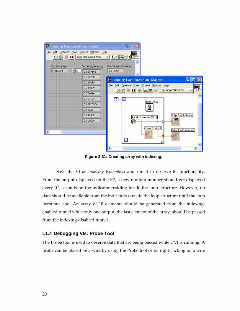
Figure 2-31: Creating array with indexing.

Save the VI as Indexing Example.vi and run it to observe its functionality.

From the output displayed on the FP, a new random number should get displayed

every 0.1 seconds on the indicator residing inside the loop structure. However, no

data should be available from the indicators outside the loop structure until the loop

iterations end. An array of 10 elements should be generated from the indexing-

enabled tunnel while only one output, the last element of the array, should be passed

from the indexing-disabled tunnel.

L1.4 Debugging VIs: Probe Tool

The Probe tool is used to observe data that are being passed while a VI is running. A

probe can be placed on a wire by using the Probe tool or by right-clicking on a wire

21

and choosing Probe from the shortcut menu. Probes can also be placed while a VI is

running.

Placing probes on wires create probe windows through which intermediate

values can be observed. A probe window can be customized. For example, showing

data of array data type via a graph makes debugging easier. To do this, right-click on

the wire where an array is being passed and choose Custom Probe » Controls »

Modern » Graph » Waveform Graph from the shortcut menu.

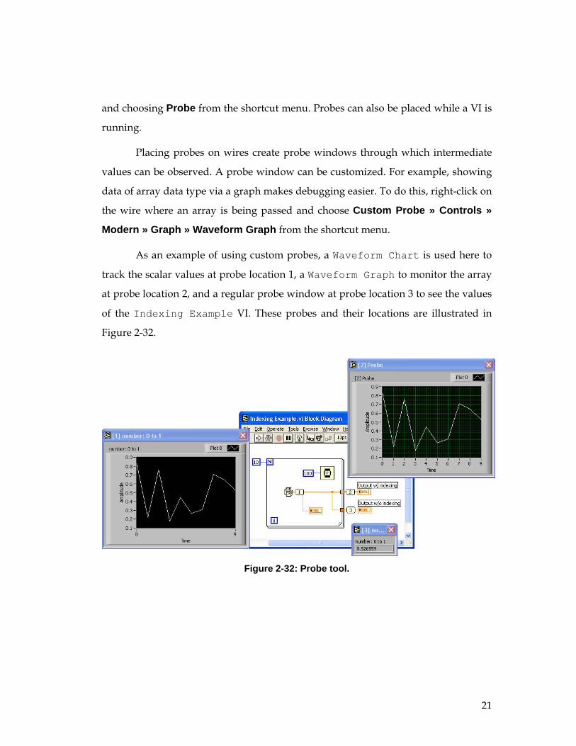
As an example of using custom probes, a Waveform Chart is used here to

track the scalar values at probe location 1, a Waveform Graph to monitor the array

at probe location 2, and a regular probe window at probe location 3 to see the values

of the Indexing Example VI. These probes and their locations are illustrated in

Figure 2-32.

Figure 2-32: Probe tool.

22

L1.5 Bibliography

[1] National Instruments, LabVIEW User Manual, Part Number 320999E-01, 2003.

L1.6 Lab Experiments

Carry out the following experiments with and without the MathScript feature of

LabVIEW 8.

1. Build a SubVI to compute the product, sum and difference of two given square

matrices A and B.

2. Build a SubVI to compute and display the roots of the quadratic equation

cbxax ++2 for given coefficients a, b and c.

3. Build a SubVI to generate the first 20 numbers of the Fibonacci sequence and

store them using an indexing array.

4. Build a SubVI to compute the sum of the first ‘n’ natural numbers for a given

value of n.