Embed Size (px)
Citation preview
COMPUTER APPLICATIONS IN THE GEOSCIENCES
In this lab, you will learn how to import topography data, display it in 3-‐D, and add several layers of other data. You will be working with topography data that has been pre-‐formatted for these types of applications – this data is SRTM (Shuttle Radar Topography Mission) data, and has a resolution of 90 m. Each data file spans 5 degrees in both longitude and latitude, and has a name corresponding to its lower-‐left corner of the grid (minimum west longitude, minimum latitude).
Setup
1. Mount the \\geobase\GEO4315 server. Create a folder in your user folder on \\geobase named Lab10.
2. Copy the file from the Instructor/Lab10 folder on \\geobase to your Lab10 folder.
Section 0. Background (read this, its important for your final project) Fledermaus is a powerful, interactive 3-‐D data visualization system that is used for a variety of geoscience applications in both research and teaching. Fledermaus has many uses, both academic and commercial, in ocean exploration, mapping, and development-‐related fields, as well as other geospatial/geoscience research and industry fields. The Fledermaus software suite allows researchers and educators to create and interact with full-‐resolution terrain and bathymetric surface models, and then integrate those surfaces with a variety of other data types to make a "scene." Users can add images, vertical imagery, ASCII points and lines, Electronic Nautical Charts (ENCs), 3-‐D models, and ESRI shape files to build attractive and easy-‐to-‐use visualizations. Users can also use Fledermaus to run profiles along a surface, do slope calculations, and create fly-‐throughs (flight paths). Users can interact with the data using a standard 3-‐button mouse or a 3-‐D navigation device (3DConnexion Space Navigator) in normal viewing mode or stereo (split-‐screen or full stereo). In the near future, Fledermaus will support the integration and display of time-‐stamped data, so that users can show things like earthquakes, sediment migration, and wave propagation over time. iView4D is a free viewer for Fledermaus format files. Users can download, view, and interact with already-‐created scenes that others have posted; flight paths
LL A B A B 1 0 1 0 FF L E D E R M A U S L E D E R M A U S 33 -- D VD V I S U A L I Z A T I O N I S U A L I Z A T I O N

COMPUTER APPLICATIONS IN THE GEOSCIENCES
created in Fledermaus can also be played back in iView4D. Before beginning the practice exercise, you should familiarize yourself with where the following four Fledermaus programs are located on your computer :
• PCs: All Programs Fledermaus-‐V7
• Macs: Navigate to: Macintosh HD Applications IVS Fledermaus-‐v7
For more information and official documentation on Fledermaus, go to: http://www.ivs3d.com/docs/v7_Reference_Manual.pdf
Step 1. Try out Fledermaus
o First you will download a pre-‐made Fledermaus file (a .scene file) from the
web. In a web browser, got to the following site: http://siovizcenter.ucsd.edu/. Click on the Library tab at the top of the page, then click on the Scene Files link on the following page.
o Scroll down and click on “Global Earthquakes”. This page provides you with some details about the data represented in the file you are about to download. Click on the link “23.3 MB” to download the file (named IDA.scene.zip) to your computer. Save it to your Lab10 folder on //geobase.
o This file is compressed (zipped), so double click on it once it has fully downloaded. Your computer should try and uncompress the file automatically – when this happens the new file you will work with will be named IDA.scene. A scene file in Fledermaus is a collection of different data layers.
o Next launch Fledermaus (v7) and open up the IDA.scene file with File Open Data Object/Scene...
o Once your file has loaded into Fledermaus, you can interactively explore the data set. Use the widget (the thing with an x-‐ and y-‐axis) to rotate and scroll bars (horizontal and vertical) to zoom.
o Turn on/off the different layers by checking/unchecking the different data set layers, which are listed in the panel below the visualization screen, left side. Note that you can right-‐click on each data layer and save individual data layers to your desktop. **This will be a particularly important tool for your final projects – you can utilize other people’s Fledermaus layers for your own projects**.
o Change the vertical exaggeration of your scene by entering different values into the Exag box (left side of visualization screen).
o Try out the other options and buttons available. If you get lost, just hit the left camera icon (vertical menu bar located in the top right corner) to return
COMPUTER APPLICATIONS IN THE GEOSCIENCES
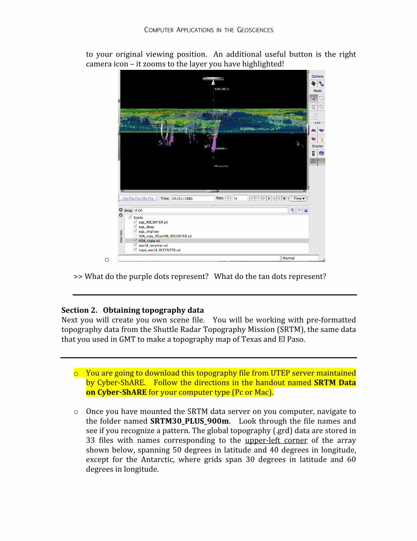
to your original viewing position. An additional useful button is the right camera icon – it zooms to the layer you have highlighted!
o >> What do the purple dots represent? What do the tan dots represent?
Section 2. Obtaining topography data Next you will create you own scene file. You will be working with pre-‐formatted topography data from the Shuttle Radar Topography Mission (SRTM), the same data that you used in GMT to make a topography map of Texas and El Paso.
o You are going to download this topography file from UTEP server maintained
by Cyber-‐ShARE. Follow the directions in the handout named SRTM Data on Cyber-ShARE for your computer type (Pc or Mac).
o Once you have mounted the SRTM data server on you computer, navigate to the folder named SRTM30_PLUS_900m. Look through the file names and see if you recognize a pattern. The global topography (.grd) data are stored in 33 files with names corresponding to the upper-‐left corner of the array shown below, spanning 50 degrees in latitude and 40 degrees in longitude, except for the Antarctic, where grids span 30 degrees in latitude and 60 degrees in longitude.

COMPUTER APPLICATIONS IN THE GEOSCIENCES
o We want the grid that covers most of west Texas. Circle this grid box above.
o The grid that corresponds to this region is named w140n40.Bathymetry.srtm.grd. Given this information, enter the min/max latitude and longitude values in the box below, representing this grid. Also copy/paste this file to your Lab10 folder. Make sure that you are actually copying the grid file, and not some empty text file. The grid file will be several Mb.
Having read the SRTM handout, please answer the following questions:
Does the 90-‐m resolution data set cover both land topography, ocean topography, or both?
Does the 900-‐m resolution data set cover both land topography, ocean topography, or both?
What is the approximate size of a 90-‐m resolution topography file, in
Mb?
COMPUTER APPLICATIONS IN THE GEOSCIENCES
What is the approximate size of a 900-‐m resolution topography file, in Mb?
If you wanted to make a map of the entire continental U.S., which data set would be more appropriate – the 90-‐m or the 900-‐m?
Step 2.1 Importing data
o Now you will import topography data file w140n40.Bathymetry.srtm.grd into the Fledermaus program. Clear the current scene with File Clear Scene.
o Next import that data file: Import Import Gridded Data (specify your
Lab10 folder, and select w140n40.Bathymetry.srtm.grd file )
o Under File Type menu, select GMT Grd, click Next
o Check that the Data Dimensions and XYZ coordinates make sense. Output Coordinate System should have Horizontal Coordinate System left on FG_WGS_84, and the Vertical Datum should say FG_Unspecified_Meters, click Next.
o Click Next on the following Z coordinates screen.
o Leave Output SD Type checked for Sonar DTM. Make sure that the SD
filename will be saved to your Lab10 folder. In the Convert and Save to SD File box, name your file SW_US.sd. (for Southwest United States). Select a colormap under Color Map using the Browse button -‐-‐ choose “gmtglobe_d.cmap” and click Open, then Finish.
It will take a while to import and create an SD file for your topography data set (be patient!). You will see a screen with topography when the import has completed. Can you identify where El Paso is? (if you can, great. If not, we’ll be adding more layers to help with this later on) Step 2.2 Adjusting colors
o Under the Color Map tab (panel beneath the topography scene), there is a button on the right named Change Colormap, which will let you try other pre-‐defined colors. Note that each time you change color maps, it will take a few seconds for Fledermaus to update (be patient).
o There are a few color maps that are particularly good for illustrating elevation changes. For regions encompassing both water bodies and
COMPUTER APPLICATIONS IN THE GEOSCIENCES
landforms, gmt_topo.cmap, is a good choice. The colors in gmt.cmap (very colorful) or gmt_globe.cmap (more natural) are also good for land-‐only color schemes.
o Alternatively, you can edit the one you currently have by clicking the Tools
button and selecting Edit CMap. If you do this, a window will pop up allowing you to either pick different elevations, or colors.
Step 2.3 Shading the topography
o Click on the Shading tab and you can experiment with the direction (circular dial) and magnitude (vertical slider) of shading to apply to your topography. Choose a setting and click Shade to see what you did. Once you have a setting that you like, you can keep the shading data by hitting the Tools button and save your shade to a file.
Step 2.4 Setting a colorbar
o To identify the elevations in your topography scene, click on the colorbar icon in the vertical menu on the right. Units are in meters.
What are the elevations? Step 2.5 Editing your DTM Almost done. The DTM in Fledermaus is your geo-‐referenced layer, typically your topography layer. Using the DTM tab, you can switch to Wireframe Surface, which will generate a mesh instead of a colored and shaded surface for the topography. In addition, you can make the layer transparent, using the Transparency slider.
__________________________________ Section 3. Adding simple layers
Next you will add a layer that for the U.S. states that will add a geographic reference to your topography data. This layer is called USA_States.sd and should be one of the files that you copied to your Lab10 folder from the Instructor folder on //geobase.
o Go File Open Data Object/Scene and select USA_States.sd o If the lines disappear beneath your topography, click on the layer name
(USA_States) in the panel on the bottom left (click to highlight), then click on the Object Attributes tab (if this tab is not obvious, select Controls Object Attributes to get a floating window). Click on the Resample and Drape button and click Okay to use 0.1 as the Sampling Interval.
o Change the color of the line to black. Click on the Change Color button to do this.

COMPUTER APPLICATIONS IN THE GEOSCIENCES
Section 4. Adding layers – ArcGIS shapefiles Here we’ll practice importing a *mystery* shapefile that you copied from the Instructor folder:
o Import Import ArcGIS Shape. Navigate to your Lab10/Myster_shape_file folder, then the select the *.shp file and click Open.
o The Import ArcGIS Shape window appears. Keep all the defaults and set the Horizontal Coordinate System to FG_WGS_84 (if its not already set) and click OK.
o Once imported, your lines may be hiding beneath your topography file. To test this, uncheck the topography data file (w140n40.Bathymetry.srtm.sd) in the panel on the bottom left corner of the Fledermaus window. You should then be able to see clusters of lines and points representing the mystery data file (= population density!)
o Change the color of this file to red. Click on the Change Color button to do
this.
o You may need to drape your lines over the topography. Click on the mysteryfile layer name in the panel on the bottom left corner of the Fledermaus window (click to highlight), then click on Resample and Drape, just as you did for the USA_States layer. If this still doesn’t reveal the mysteryfile lines, click on the Set Heights button and enter 2000. This will pull the lines up above the topography data in most regions.

COMPUTER APPLICATIONS IN THE GEOSCIENCES
Section 5. Extracting a topography profile
o Under the Data Sets tab, click on the topography layer (w140n40.Bathymetry.srtm.sd), then hold down the ctrl key and drag your mouse across your topography scene, anywhere that you like. I’d recommend playing with this tool a few times to see how the profiles vary as you move right to left, north to south, and vice versa.
o A Profiling window should appear, showing a vertical profile, or cross-‐section of the topography that your line just sampled. The units of your profile (in meters) are displayed along both the horizontal axis and the vertical axis. The example below shows a profile extracted across parts of Texas, from the west to the east.

COMPUTER APPLICATIONS IN THE GEOSCIENCES
o You can save the values of your profile to a file with the extension .pfl. To do this, click on the Tools button, select Save Profile. You can go with the default sampling interval (meters), or you can edit this to reflect a higher value (so sampling fewer points, which will yield a rough profile) or a lower value (so sampling more points, which will yield a smooth profile). Save your file as MyProfile.pfl in your Lab10 folder.
o Now take a quick peek at your MyProfile.pfl file by opening it either in a NotePad (PCs) or Text Edit (Macs). An example profile is shown below. The 1st column is the horizontal profile axis values, in meters. The 2nd and 3rd columns are longitude/latitude. The 4th column is the topography elevations, the vertical profile axis values, in meters.
o Back in Fledermaus, note that you can also save a image of your profile using the Tools Save Profile Image. Save your profile image as MyProfileImage in your Lab10 folder.
Section 6. Saving
o To save all of your data layers to one file, make sure that all of your data layers are checked and save your work to a .scene file: File Save Scene. Name your file MySWUSData.scene and save it to your Lab10 folder.
o Zoom to a place that you’d like to save an image of, and do so by going File Screen Capture. You may want to first get rid of your widget (the turn navigation tool) by clicking on the vertical menu button on the right side of the Fledermaus window (under Display). Save the file as a JPG, named SWUS_zoom.jpg and save to your Lab10 folder. Magnification of 1 should be fine.
Place a copy of the following files to the DROPBOX for full credit: MyProfile.pfl, MyProfileImage, SWUS_zoom.jpg.