Lab 3: Digitizing in ArcGIS Pro - giscourses.cfans.umn.edu · GIS Fundamentals: Introduction to GIS Lab 3, Digitizing 1 Lab 3: Digitizing in ArcGIS Pro What You’ll Learn: ... GIS

GIS Fundamentals: Introduction to GIS Lab 3, Digitizing

1

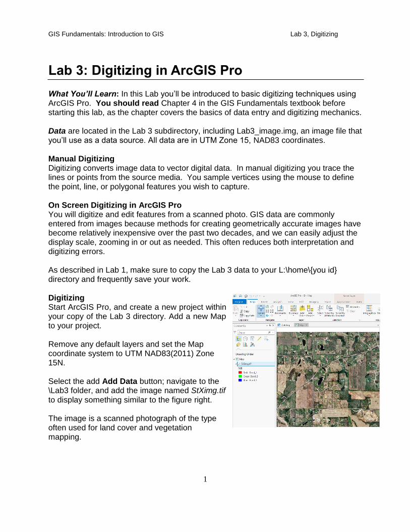
Lab 3: Digitizing in ArcGIS Pro What You’ll Learn: In this Lab you’ll be introduced to basic digitizing techniques using ArcGIS Pro. You should read Chapter 4 in the GIS Fundamentals textbook before starting this lab, as the chapter covers the basics of data entry and digitizing mechanics. Data are located in the Lab 3 subdirectory, including Lab3_image.img, an image file that you’ll use as a data source. All data are in UTM Zone 15, NAD83 coordinates. Manual Digitizing Digitizing converts image data to vector digital data. In manual digitizing you trace the lines or points from the source media. You sample vertices using the mouse to define the point, line, or polygonal features you wish to capture. On Screen Digitizing in ArcGIS Pro You will digitize and edit features from a scanned photo. GIS data are commonly entered from images because methods for creating geometrically accurate images have become relatively inexpensive over the past two decades, and we can easily adjust the display scale, zooming in or out as needed. This often reduces both interpretation and digitizing errors. As described in Lab 1, make sure to copy the Lab 3 data to your L:\home\{you id} directory and frequently save your work. Digitizing Start ArcGIS Pro, and create a new project within your copy of the Lab 3 directory. Add a new Map to your project. Remove any default layers and set the Map coordinate system to UTM NAD83(2011) Zone 15N. Select the add Add Data button; navigate to the \Lab3 folder, and add the image named StXimg.tif to display something similar to the figure right. The image is a scanned photograph of the type often used for land cover and vegetation mapping.


2

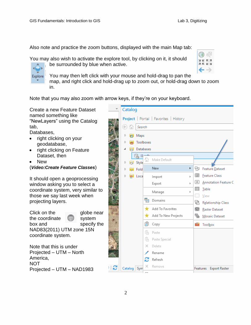
Also note and practice the zoom buttons, displayed with the main Map tab: You may also wish to activate the explore tool, by clicking on it, it should

be surrounded by blue when active. You may then left click with your mouse and hold-drag to pan the map, and right click and hold-drag up to zoom out, or hold-drag down to zoom in.

Note that you may also zoom with arrow keys, if they’re on your keyboard. Create a new Feature Dataset named something like “NewLayers” using the Catalog tab, Databases,

right clicking on your geodatabase,

right clicking on Feature Dataset, then

New (Video:Create Feature Classes) It should open a geoprocessing window asking you to select a coordinate system, very similar to those we say last week when projecting layers. Click on the globe near the coordinate system box and specify the NAD83(2011) UTM zone 15N coordinate system. Note that this is under Projected – UTM – North America, NOT Projected – UTM – NAD1983


3

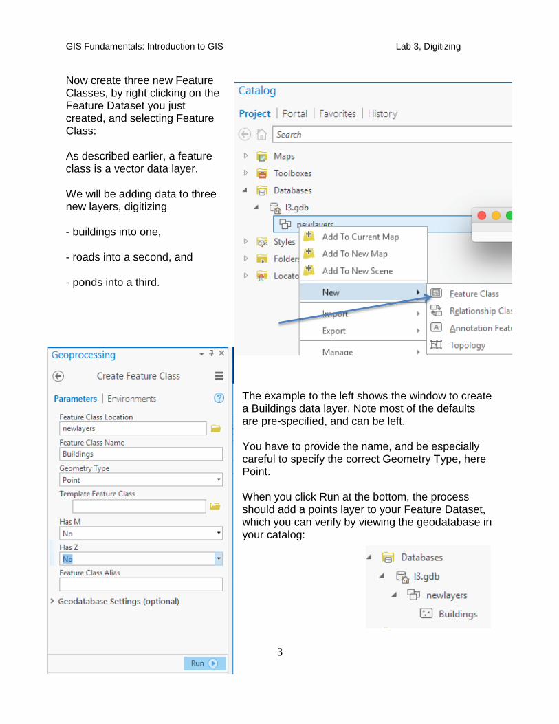
Now create three new Feature Classes, by right clicking on the Feature Dataset you just created, and selecting Feature Class: As described earlier, a feature class is a vector data layer. We will be adding data to three new layers, digitizing - buildings into one, - roads into a second, and - ponds into a third.

The example to the left shows the window to create a Buildings data layer. Note most of the defaults are pre-specified, and can be left. You have to provide the name, and be especially careful to specify the correct Geometry Type, here Point. When you click Run at the bottom, the process should add a points layer to your Feature Dataset, which you can verify by viewing the geodatabase in your catalog:


4

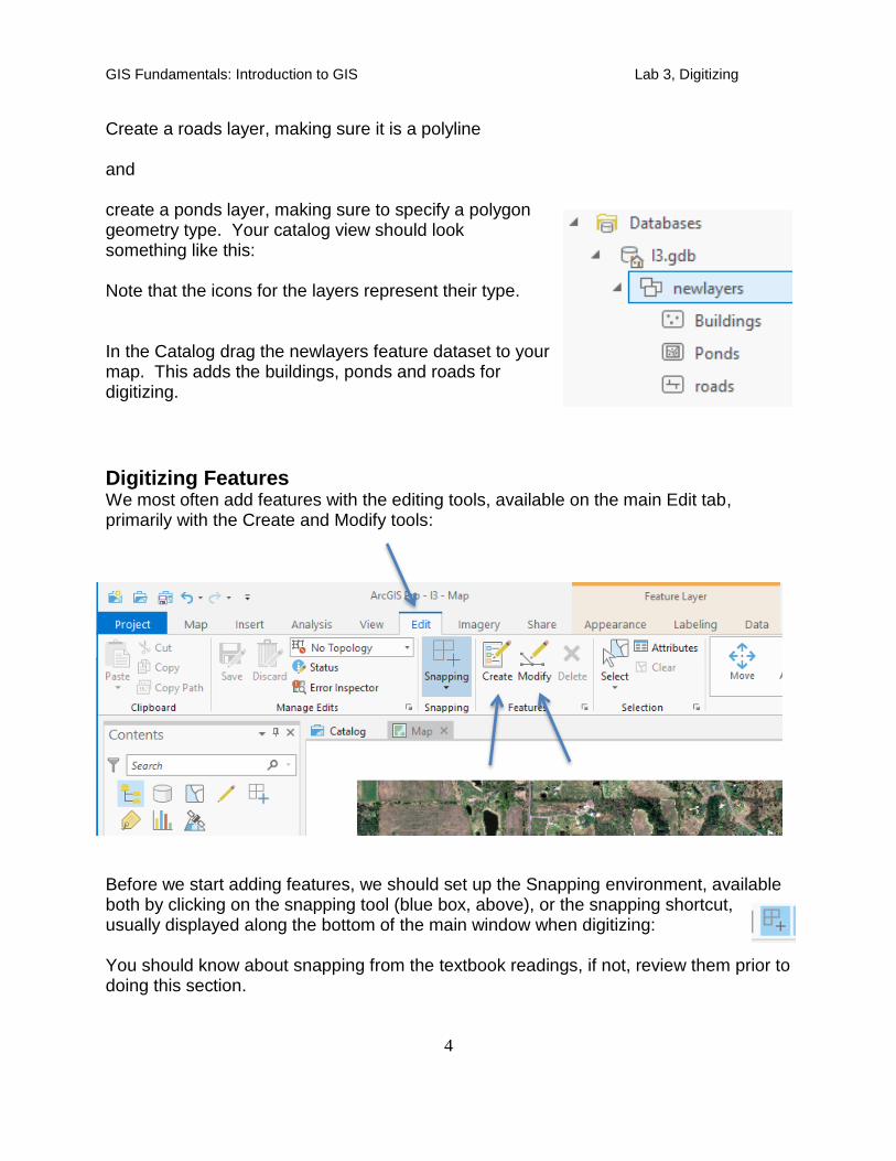
Create a roads layer, making sure it is a polyline and create a ponds layer, making sure to specify a polygon geometry type. Your catalog view should look something like this: Note that the icons for the layers represent their type. In the Catalog drag the newlayers feature dataset to your map. This adds the buildings, ponds and roads for digitizing.

Digitizing Features We most often add features with the editing tools, available on the main Edit tab, primarily with the Create and Modify tools:

Before we start adding features, we should set up the Snapping environment, available both by clicking on the snapping tool (blue box, above), or the snapping shortcut, usually displayed along the bottom of the main window when digitizing: You should know about snapping from the textbook readings, if not, review them prior to doing this section.


5

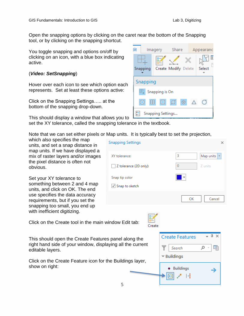
Open the snapping options by clicking on the caret near the bottom of the Snapping tool, or by clicking on the snapping shortcut. You toggle snapping and options on/off by clicking on an icon, with a blue box indicating active. (Video: SetSnapping) Hover over each icon to see which option each represents. Set at least these options active: Click on the Snapping Settings….. at the bottom of the snapping drop-down. This should display a window that allows you to set the XY tolerance, called the snapping tolerance in the textbook. Note that we can set either pixels or Map units. It is typically best to set the projection, which also specifies the map units, and set a snap distance in map units. If we have displayed a mix of raster layers and/or images the pixel distance is often not obvious. Set your XY tolerance to something between 2 and 4 map units, and click on OK. The end use specifies the data accuracy requirements, but if you set the snapping too small, you end up with inefficient digitizing. Click on the Create tool in the main window Edit tab: This should open the Create Features panel along the right hand side of your window, displaying all the current editable layers. Click on the Create Feature icon for the Buildings layer, show on right:


6

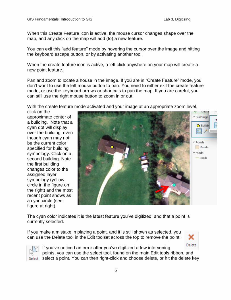
When this Create Feature icon is active, the mouse cursor changes shape over the map, and any click on the map will add (to) a new feature. You can exit this “add feature” mode by hovering the cursor over the image and hitting the keyboard escape button, or by activating another tool. When the create feature icon is active, a left click anywhere on your map will create a new point feature. Pan and zoom to locate a house in the image. If you are in “Create Feature” mode, you don’t want to use the left mouse button to pan. You need to either exit the create feature mode, or use the keyboard arrows or shortcuts to pan the map. If you are careful, you can still use the right mouse button to zoom in or out. With the create feature mode activated and your image at an appropriate zoom level, click on the approximate center of a building. Note that a cyan dot will display over the building, even though cyan may not be the current color specified for building symbology. Click on a second building. Note the first building changes color to the assigned layer symbology (yellow circle in the figure on the right) and the most recent point shows as a cyan circle (see figure at right). The cyan color indicates it is the latest feature you’ve digitized, and that a point is currently selected. If you make a mistake in placing a point, and it is still shown as selected, you can use the Delete tool in the Edit toolset across the top to remove the point:

If you’ve noticed an error after you’ve digitized a few intervening points, you can use the select tool, found on the main Edit tools ribbon, and select a point. You can then right-click and choose delete, or hit the delete key


7

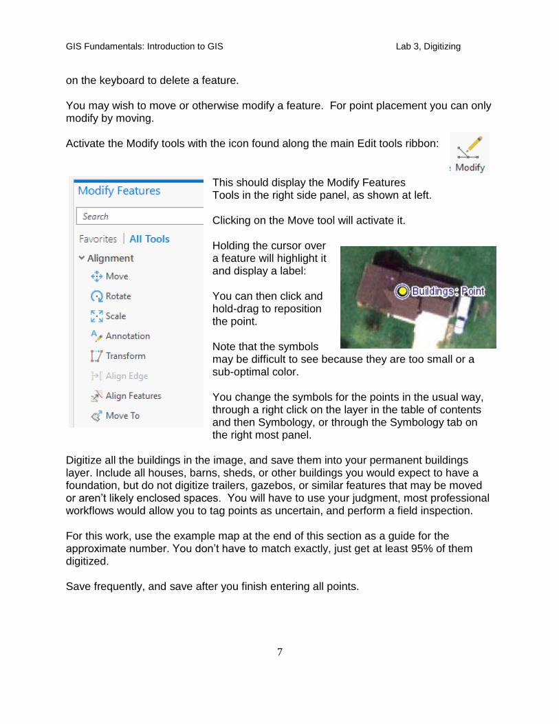
on the keyboard to delete a feature. You may wish to move or otherwise modify a feature. For point placement you can only modify by moving. Activate the Modify tools with the icon found along the main Edit tools ribbon:

This should display the Modify Features Tools in the right side panel, as shown at left. Clicking on the Move tool will activate it. Holding the cursor over a feature will highlight it and display a label: You can then click and hold-drag to reposition the point. Note that the symbols may be difficult to see because they are too small or a sub-optimal color. You change the symbols for the points in the usual way, through a right click on the layer in the table of contents and then Symbology, or through the Symbology tab on the right most panel.

Digitize all the buildings in the image, and save them into your permanent buildings layer. Include all houses, barns, sheds, or other buildings you would expect to have a foundation, but do not digitize trailers, gazebos, or similar features that may be moved or aren’t likely enclosed spaces. You will have to use your judgment, most professional workflows would allow you to tag points as uncertain, and perform a field inspection. For this work, use the example map at the end of this section as a guide for the approximate number. You don’t have to match exactly, just get at least 95% of them digitized. Save frequently, and save after you finish entering all points.


8

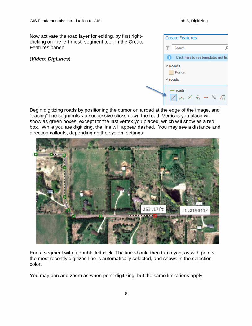
Now activate the road layer for editing, by first right-clicking on the left-most, segment tool, in the Create Features panel: (Video: DigLines) Begin digitizing roads by positioning the cursor on a road at the edge of the image, and “tracing” line segments via successive clicks down the road. Vertices you place will show as green boxes, except for the last vertex you placed, which will show as a red box. While you are digitizing, the line will appear dashed. You may see a distance and direction callouts, depending on the system settings:

End a segment with a double left click. The line should then turn cyan, as with points, the most recently digitized line is automatically selected, and shows in the selection color. You may pan and zoom as when point digitizing, but the same limitations apply.


9

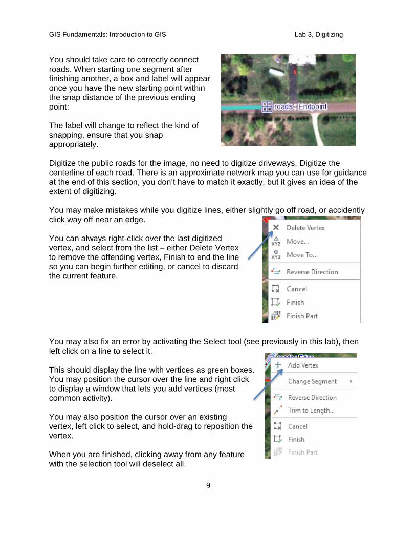
You should take care to correctly connect roads. When starting one segment after finishing another, a box and label will appear once you have the new starting point within the snap distance of the previous ending point: The label will change to reflect the kind of snapping, ensure that you snap appropriately. Digitize the public roads for the image, no need to digitize driveways. Digitize the centerline of each road. There is an approximate network map you can use for guidance at the end of this section, you don’t have to match it exactly, but it gives an idea of the extent of digitizing. You may make mistakes while you digitize lines, either slightly go off road, or accidently click way off near an edge. You can always right-click over the last digitized vertex, and select from the list – either Delete Vertex to remove the offending vertex, Finish to end the line so you can begin further editing, or cancel to discard the current feature. You may also fix an error by activating the Select tool (see previously in this lab), then left click on a line to select it. This should display the line with vertices as green boxes. You may position the cursor over the line and right click to display a window that lets you add vertices (most common activity). You may also position the cursor over an existing vertex, left click to select, and hold-drag to reposition the vertex. When you are finished, clicking away from any feature with the selection tool will deselect all.


10

A fuller set of tools is accessed through the Modify button on the main Edit ribbon.

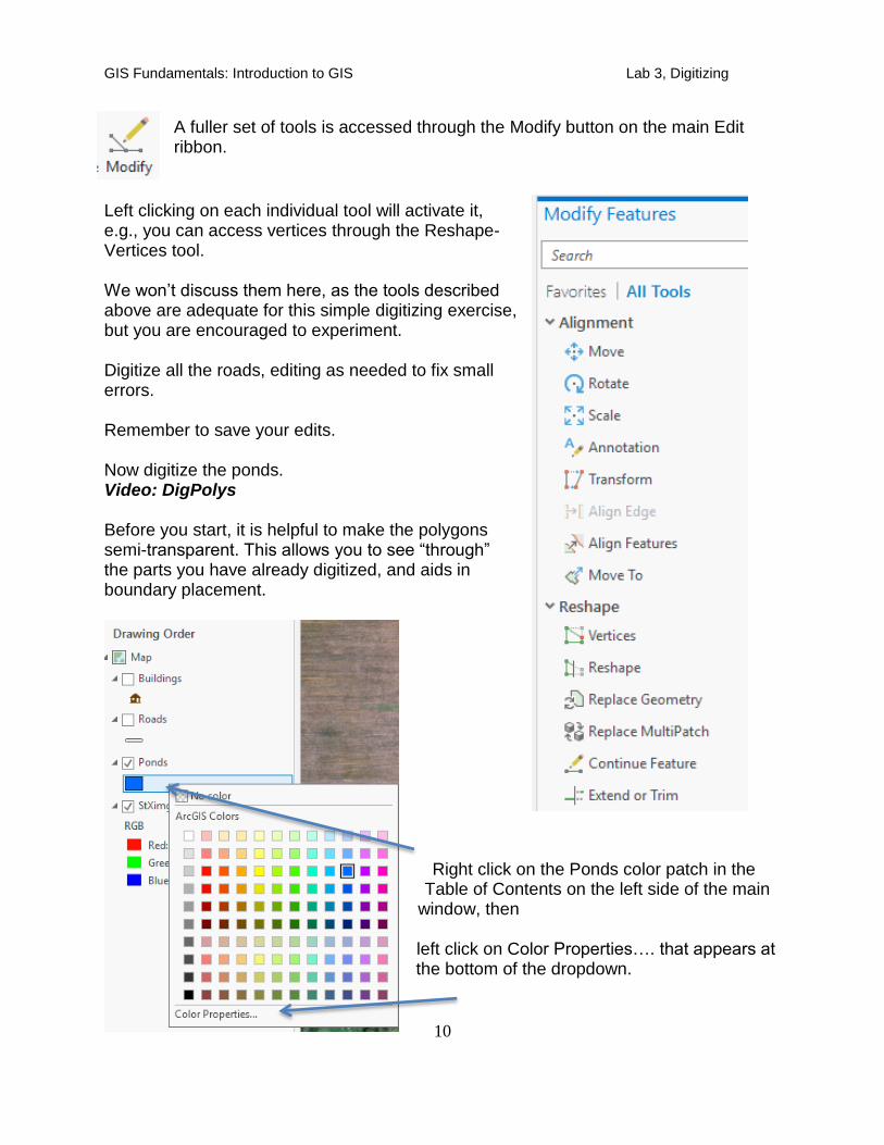
Left clicking on each individual tool will activate it, e.g., you can access vertices through the Reshape-Vertices tool. We won’t discuss them here, as the tools described above are adequate for this simple digitizing exercise, but you are encouraged to experiment. Digitize all the roads, editing as needed to fix small errors. Remember to save your edits. Now digitize the ponds. Video: DigPolys Before you start, it is helpful to make the polygons semi-transparent. This allows you to see “through” the parts you have already digitized, and aids in boundary placement.

Right click on the Ponds color patch in the

Table of Contents on the left side of the main window, then left click on Color Properties…. that appears at the bottom of the dropdown.


11

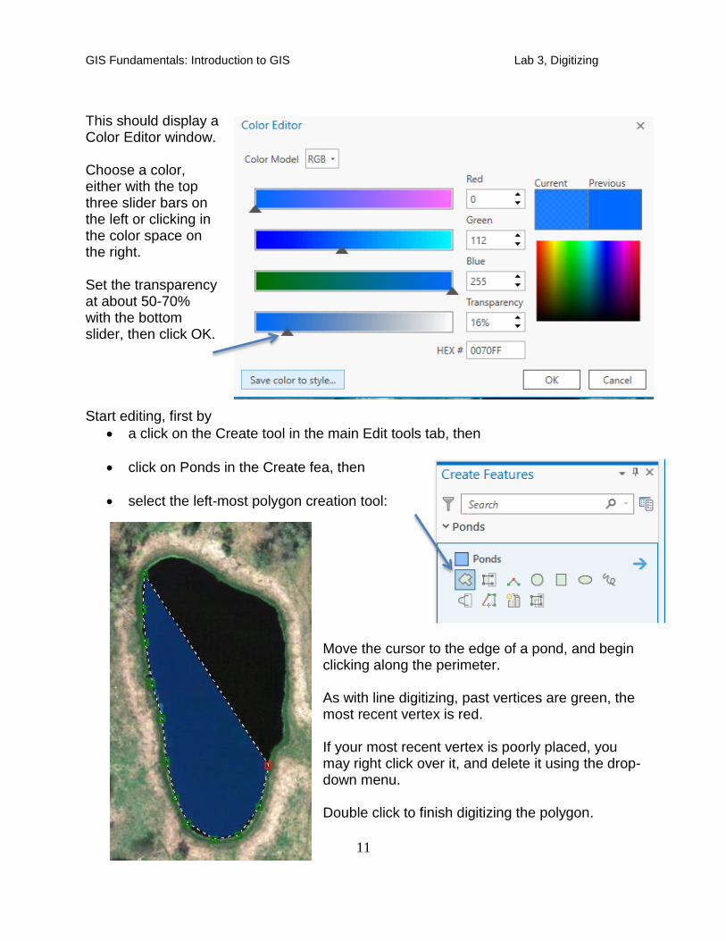
This should display a Color Editor window. Choose a color, either with the top three slider bars on the left or clicking in the color space on the right. Set the transparency at about 50-70% with the bottom slider, then click OK. Start editing, first by

a click on the Create tool in the main Edit tools tab, then

click on Ponds in the Create fea, then

select the left-most polygon creation tool: Move the cursor to the edge of a pond, and begin clicking along the perimeter. As with line digitizing, past vertices are green, the most recent vertex is red. If your most recent vertex is poorly placed, you may right click over it, and delete it using the drop-down menu. Double click to finish digitizing the polygon.


12

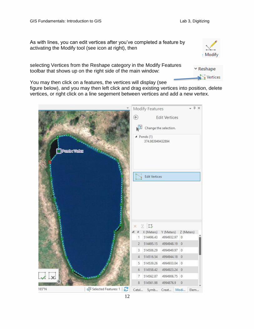
As with lines, you can edit vertices after you’ve completed a feature by activating the Modify tool (see icon at right), then selecting Vertices from the Reshape category in the Modify Features toolbar that shows up on the right side of the main window: You may then click on a features, the vertices will display (see figure below), and you may then left click and drag existing vertices into position, delete vertices, or right click on a line segement between vertices and add a new vertex.


13

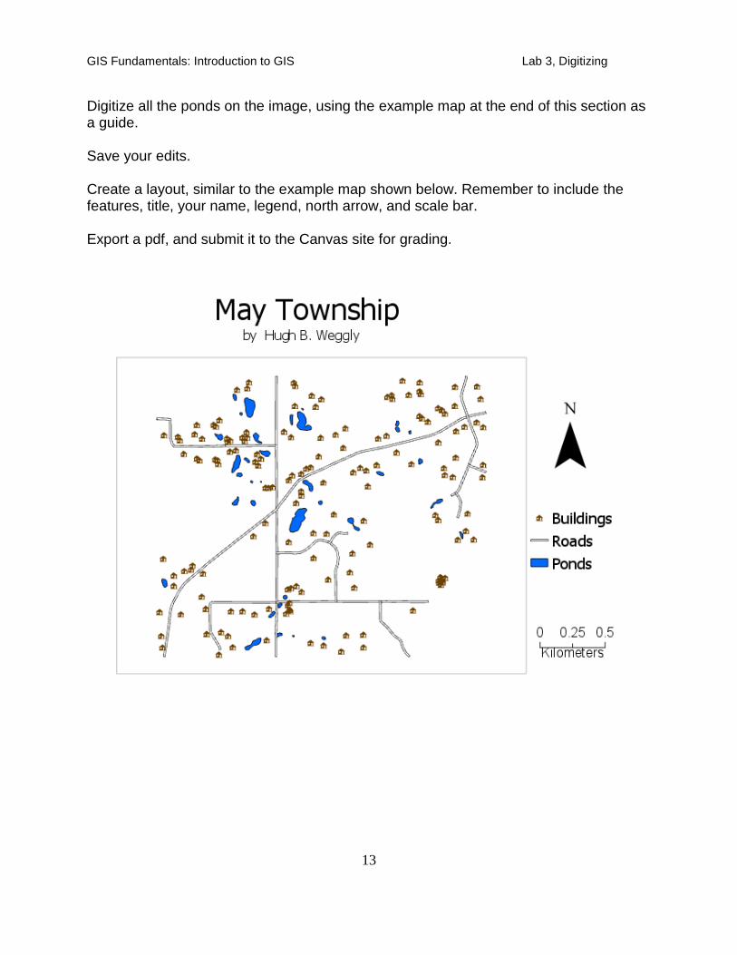
Digitize all the ponds on the image, using the example map at the end of this section as a guide. Save your edits.

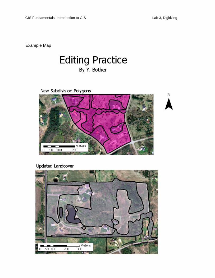
Create a layout, similar to the example map shown below. Remember to include the features, title, your name, legend, north arrow, and scale bar. Export a pdf, and submit it to the Canvas site for grading.


14

Adding and Editing (Note: read and study this section as you will need to use these techniques later in the lab; You do not need to do this practice exercise or turn anything in from this section; If you do want to examine the data files used in this example they are in \Lab3\l3\testdata.gdb)

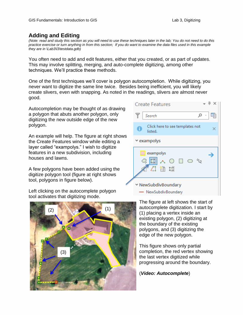
You often need to add and edit features, either that you created, or as part of updates. This may involve splitting, merging, and auto-complete digitizing, among other techniques. We’ll practice these methods. One of the first techniques we’ll cover is polygon autocompletion. While digitizing, you never want to digitize the same line twice. Besides being inefficient, you will likely create slivers, even with snapping. As noted in the readings, slivers are almost never good. Autocompletion may be thought of as drawing a polygon that abuts another polygon, only digitizing the new outside edge of the new polygon. An example will help. The figure at right shows the Create Features window while editing a layer called “exampolys.” I wish to digitize features in a new subdivision, including houses and lawns. A few polygons have been added using the digitize polygon tool (figure at right shows tool, polygons in figure below). Left clicking on the autocomplete polygon tool activates that digitizing mode.

The figure at left shows the start of autocomplete digitization. I start by (1) placing a vertex inside an existing polygon, (2) digitizing at the boundary of the existing polygons, and (3) digitizing the edge of the new polygon. This figure shows only partial completion, the red vertex showing the last vertex digitized while progressing around the boundary. (Video: Autocomplete)

(1) (2)

(3)


15

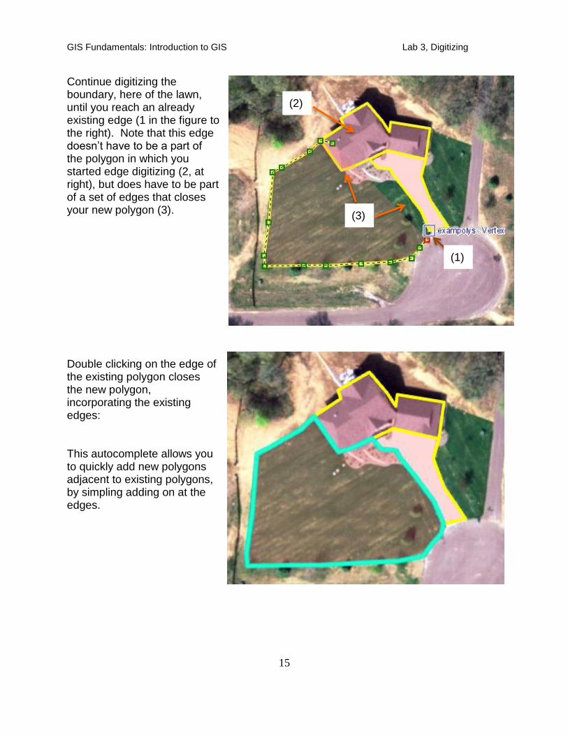
Continue digitizing the boundary, here of the lawn, until you reach an already existing edge (1 in the figure to the right). Note that this edge doesn’t have to be a part of the polygon in which you started edge digitizing (2, at right), but does have to be part of a set of edges that closes your new polygon (3). Double clicking on the edge of the existing polygon closes the new polygon, incorporating the existing edges: This autocomplete allows you to quickly add new polygons adjacent to existing polygons, by simpling adding on at the edges.

(1)

(2)

(3)


16

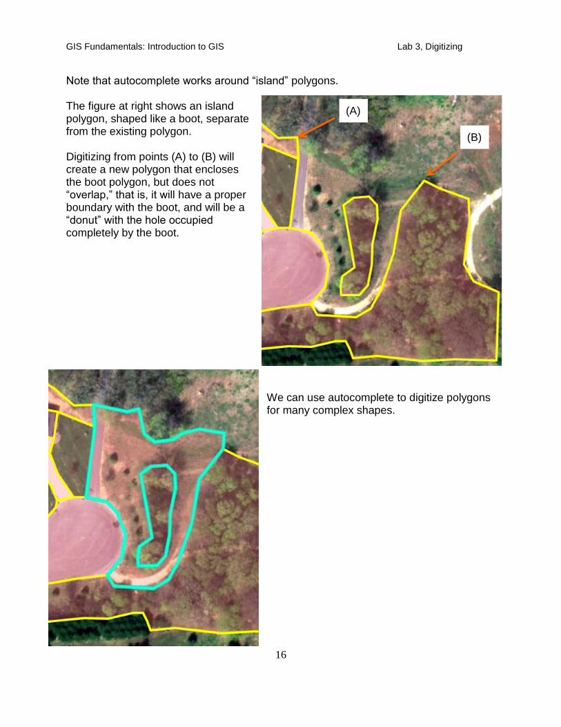
Note that autocomplete works around “island” polygons. The figure at right shows an island polygon, shaped like a boot, separate from the existing polygon. Digitizing from points (A) to (B) will create a new polygon that encloses the boot polygon, but does not “overlap,” that is, it will have a proper boundary with the boot, and will be a “donut” with the hole occupied completely by the boot.

We can use autocomplete to digitize polygons for many complex shapes.

(A)

(B)


17

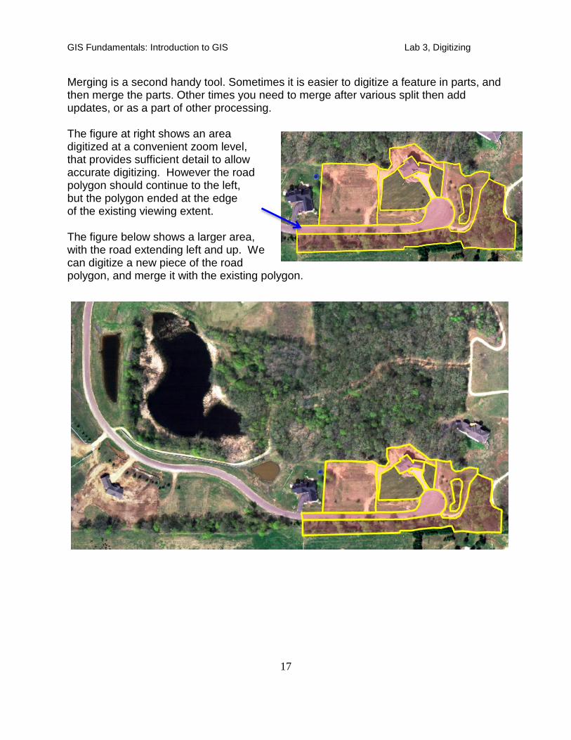
Merging is a second handy tool. Sometimes it is easier to digitize a feature in parts, and then merge the parts. Other times you need to merge after various split then add updates, or as a part of other processing. The figure at right shows an area digitized at a convenient zoom level, that provides sufficient detail to allow accurate digitizing. However the road polygon should continue to the left, but the polygon ended at the edge of the existing viewing extent. The figure below shows a larger area, with the road extending left and up. We can digitize a new piece of the road polygon, and merge it with the existing polygon.


18

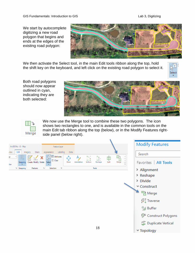
We start by autocomplete digitizing a new road polygon that begins and ends at the edges of the existing road polygon: We then activate the Select tool, in the main Edit tools ribbon along the top, hold the shift key on the keyboard, and left click on the existing road polygon to select it.

Both road polygons should now appear outlined in cyan, indicating they are both selected:

We now use the Merge tool to combine these two polygons. The icon shows two rectangles to one, and is available in the common tools on the main Edit tab ribbon along the top (below), or in the Modify Features right-side panel (below right).


19

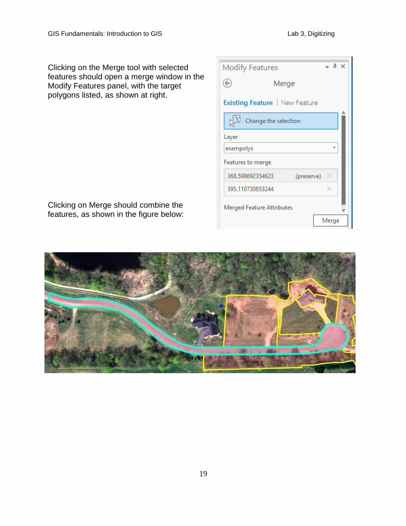
Clicking on the Merge tool with selected features should open a merge window in the Modify Features panel, with the target polygons listed, as shown at right. Clicking on Merge should combine the features, as shown in the figure below:


20

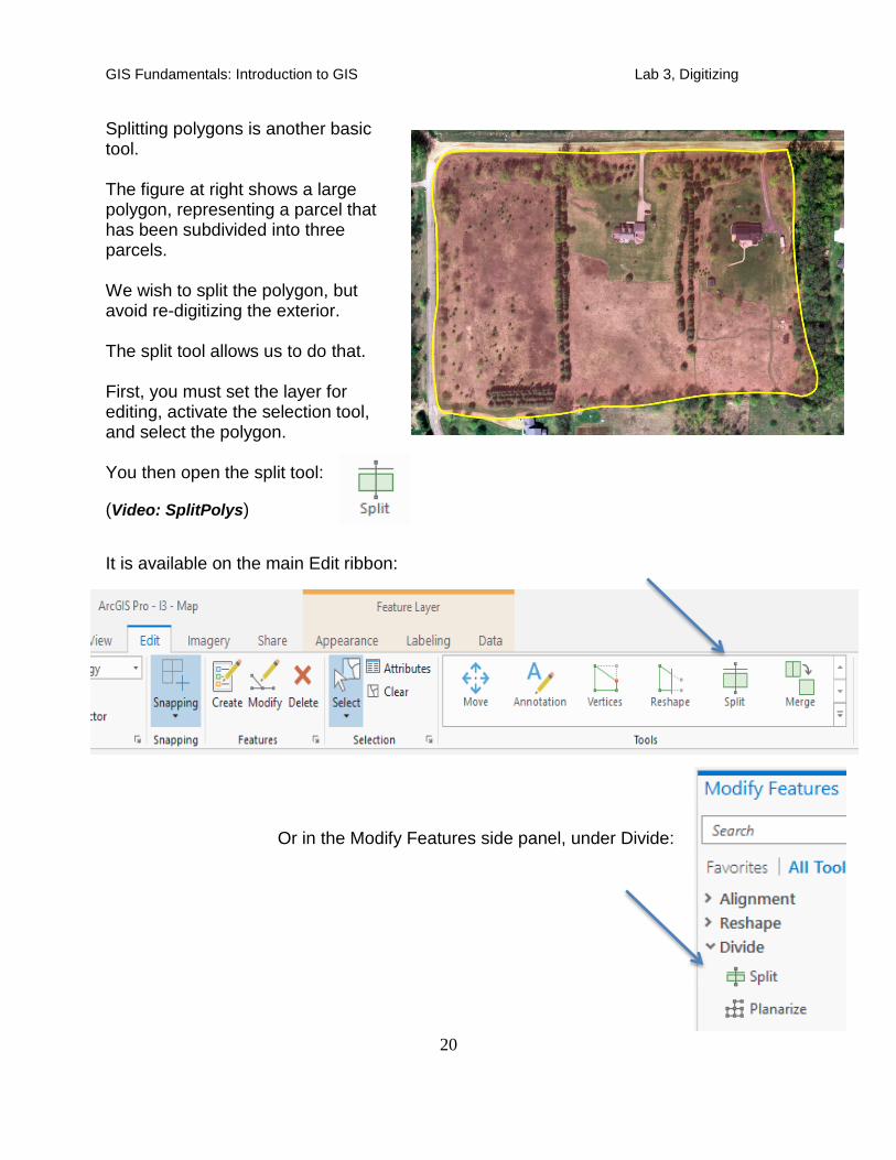
Splitting polygons is another basic tool. The figure at right shows a large polygon, representing a parcel that has been subdivided into three parcels. We wish to split the polygon, but avoid re-digitizing the exterior. The split tool allows us to do that. First, you must set the layer for editing, activate the selection tool, and select the polygon. You then open the split tool:

(Video: SplitPolys)

It is available on the main Edit ribbon:

Or in the Modify Features side panel, under Divide:


21

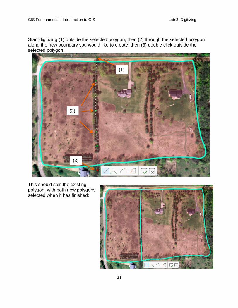
Start digitizing (1) outside the selected polygon, then (2) through the selected polygon along the new boundary you would like to create, then (3) double click outside the selected polygon.

This should split the existing polygon, with both new polygons selected when it has finished:

(1)

(3)

(2)


22

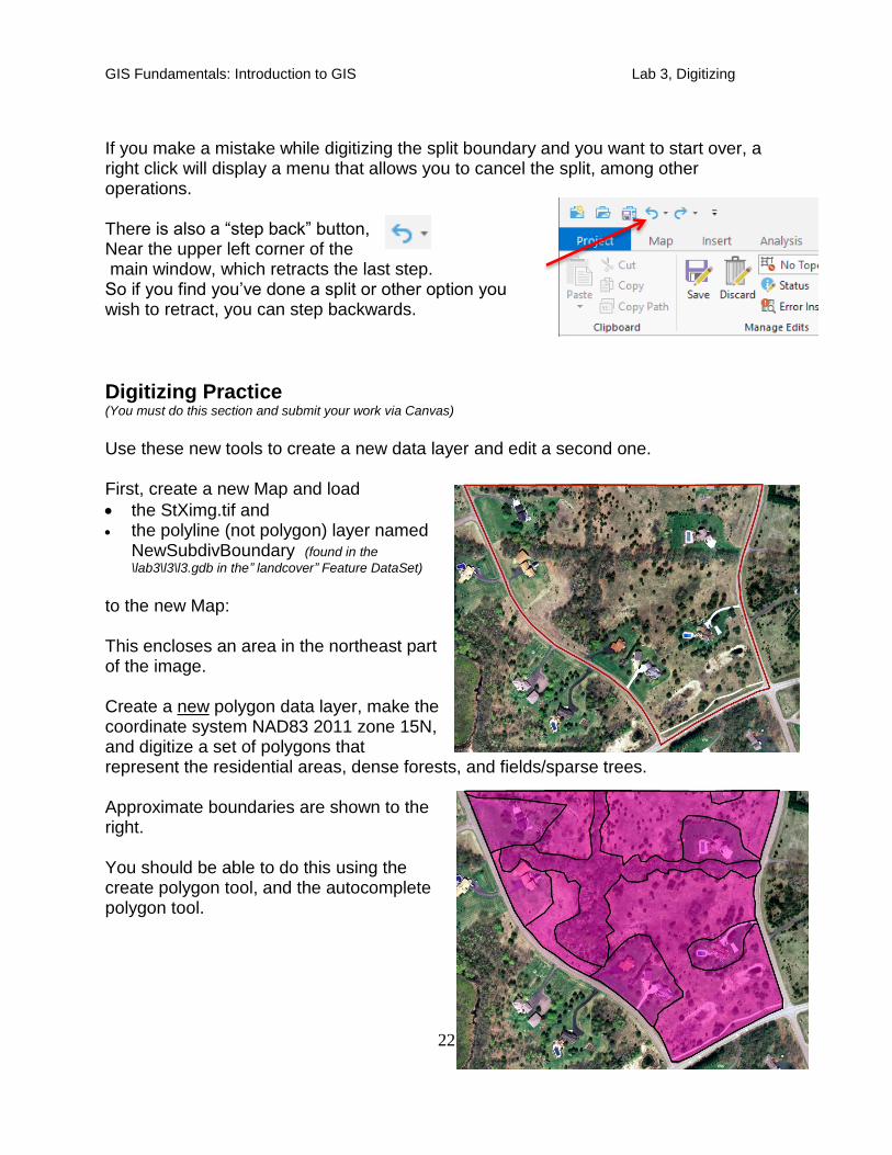
If you make a mistake while digitizing the split boundary and you want to start over, a right click will display a menu that allows you to cancel the split, among other operations. There is also a “step back” button, Near the upper left corner of the main window, which retracts the last step. So if you find you’ve done a split or other option you wish to retract, you can step backwards.

Digitizing Practice (You must do this section and submit your work via Canvas)

Use these new tools to create a new data layer and edit a second one. First, create a new Map and load

the StXimg.tif and the polyline (not polygon) layer named

NewSubdivBoundary (found in the

\lab3\l3\l3.gdb in the” landcover” Feature DataSet)

to the new Map: This encloses an area in the northeast part of the image. Create a new polygon data layer, make the coordinate system NAD83 2011 zone 15N, and digitize a set of polygons that represent the residential areas, dense forests, and fields/sparse trees. Approximate boundaries are shown to the right. You should be able to do this using the create polygon tool, and the autocomplete polygon tool.


23

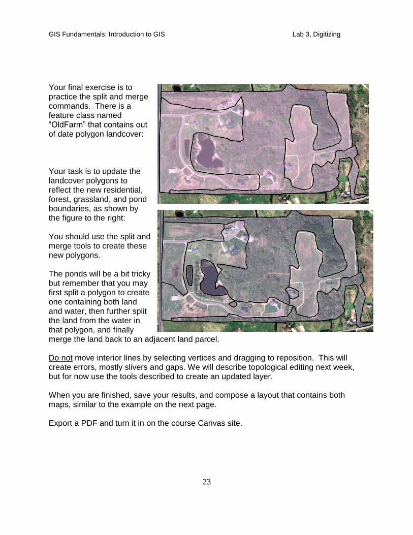
Your final exercise is to practice the split and merge commands. There is a feature class named “OldFarm” that contains out of date polygon landcover: Your task is to update the landcover polygons to reflect the new residential, forest, grassland, and pond boundaries, as shown by the figure to the right: You should use the split and merge tools to create these new polygons. The ponds will be a bit tricky but remember that you may first split a polygon to create one containing both land and water, then further split the land from the water in that polygon, and finally merge the land back to an adjacent land parcel. Do not move interior lines by selecting vertices and dragging to reposition. This will create errors, mostly slivers and gaps. We will describe topological editing next week, but for now use the tools described to create an updated layer. When you are finished, save your results, and compose a layout that contains both maps, similar to the example on the next page. Export a PDF and turn it in on the course Canvas site.


24

Example Map

Documents

Lab 3: Digitizing in ArcGIS Pro - giscourses.cfans.umn.edu · GIS Fundamentals: Introduction to GIS Lab 3, Digitizing 1 Lab 3: Digitizing in ArcGIS Pro What You’ll Learn: ... GIS