Lab on a Chip - C2N – Accueil reactors, called continuous stirred tank reactors (CSTR), have been instrumental for investigating the dynamics of out-of-equilibrium chemical processes,

Cite this: DOI: 10.1039/c2lc40649g

A nanoliter-scale open chemical reactor3

Received 7th June 2012,Accepted 7th November 2012

DOI: 10.1039/c2lc40649g

www.rsc.org/loc

Jean-Christophe Galas,* Anne-Marie Haghiri-Gosnet and Andre Estevez-Torres*

An open chemical reactor is a container that exchanges matter with the exterior. Well-mixed open

chemical reactors, called continuous stirred tank reactors (CSTR), have been instrumental for investigating

the dynamics of out-of-equilibrium chemical processes, such as oscillations, bistability, and chaos. Here, we

introduce a microfluidic CSTR, called mCSTR, that reduces reagent consumption by six orders of magnitude.

It consists of an annular reactor with four inlets and one outlet fabricated in PDMS using multi-layer soft

lithography. A monolithic peristaltic pump feeds fresh reagents into the reactor through the inlets. After

each injection the content of the reactor is continuously mixed with a second peristaltic pump. The

efficiency of the mCSTR is experimentally characterized using a bromate, sulfite, ferrocyanide pH oscillator.

Simulations accounting for the digital injection process are in agreement with experimental results. The

low consumption of the mCSTR will be advantageous for investigating out-of-equilibrium dynamics of

chemical processes involving biomolecules. These studies have been scarce so far because a miniaturized

version of a CSTR was not available.

1. Introduction

The systemic view of biological processes has regainedstrength with the advent, in the last twenty years, of powerfulinstrumental techniques such as genotyping,1 fluorescentproteins,2 or high performance microscopy.3 Throughout theprocess it has been shown experimentally that many of thecomplex behaviours that we marvel at in living cells arecontrolled by networks of chemical reactions: gene networks,signalling protein networks and metabolic networks.4–6 Thesenetworks are maintained out of equilibrium and theirfunctional response depends on two characteristics: theirtopology, i.e. how many nodes there are and which isconnected to which, and their coupling strengths, i.e. whatdynamics link two nodes. It appears that the topology may bedetermined experimentally7 but measuring the rates of thechemical process linking two nodes is much more difficult.We anticipate that studying the dynamics of purifiedbiological networks in highly controlled environments outsideof cells will help to understand how complexity emerges inbiology.8 Moreover, synthesizing in vitro networks with diversedynamic behaviours is expected to open new endeavours inmaterial sciences and in molecular computation,9 i.e. assem-blies of molecules that are able to process information andmake non-trivial decisions depending on their environment.

The discipline of non-linear chemistry has, from the 1970sto the 1990s, provided a rigorous theoretical corpus and asheer diversity of experimental observations on the dynamicsof chemical systems far from equilibrium.10 The systemsstudied in non-linear chemistry are networks of inorganicchemical reactions, principally variations around the classicalBelousov-Zhabotinsky oscillator. In contrast to biologicalreaction networks, we have a good mechanistic descriptionof these inorganic systems and a precise measurement of theirdynamic rates. First, this is because inorganic networks aresignificantly smaller and second, it is simpler to measureconcentrations and rate constants of chemical species withintubes than inside living cells. However, inorganic reactions arehard to assemble in networks with predefined dynamicbehaviours and, in this regard, synthetic biology has donebetter than inorganic chemistry.11,12 In the last ten years anintermediate strategy has emerged. It harnesses the predict-able reactivity of certain biomolecules, notably nucleic acidsand enzymes, to assemble reaction networks with controlleddynamic behaviours outside of cells. This direction was startedby the seminal paper of Yurke and coworkers13 and reached alandmark in 2011 when Rondelez and Winfree, together withtheir coworkers, independently synthesized the first engi-neered chemical system that is able to oscillate in a closedreactor.14,15

To study the dynamics of either purified biological networksor synthetic reaction networks using biomolecules one needs anopen chemical reactor that keeps the system far fromequilibrium. In this regard, microfluidics is the technology ofchoice because it provides a precise spatiotemporal16,17 controlof the concentrations of reagents with, typically, 1 mm and 1 s

Laboratoire de photonique et de nanostructures, CNRS, route de Nozay, 91460

Marcoussis, France. E-mail: [email protected];

[email protected]

3 Electronic Supplementary Information (ESI) available. See DOI: 10.1039/c2lc40649g

Lab on a Chip

PAPER

This journal is � The Royal Society of Chemistry 2012 Lab Chip

Dow

nloa

ded

on 1

2 D

ecem

ber

2012

Publ

ishe

d on

09

Nov

embe

r 20

12 o

n ht

tp://

pubs

.rsc

.org

| do

i:10.

1039

/C2L

C40

649G

View Article OnlineView Journal

http://dx.doi.org/10.1039/c2lc40649g


http://pubs.rsc.org/en/journals/journal/LC

resolution. Microfluidics has, however, stayed relatively quiet inthe development of tools for studying far-from-equilibriumchemical systems. In 2004 Ginn et al. were the first to studychemical waves within microfluidic devices.18 In a series ofremarkable papers, Ismagilov and collaborators coupled micro-fluidic design and non-linear inorganic reactions to artificiallymimic the spatio-temporal dynamics of blood clotting.19,20

More recently, Epstein and collaborators encapsulated theBelousov-Zhabotinsky reaction into arrays of water-in-oildroplets and showed the spatial coupling of these microreactorsthrough the diffusion of bromine, which is soluble in the oilphase.21 A miniaturized version of the continuous stirred tankreactor (CSTR), an open reactor that revolutionized theinvestigation of non-linear chemical reactions ,22–24 has neverbeen demonstrated. The implementation of such a device is theobjective of this work: we used an annular reactor, withinjection and mixing actuated through monolithic PDMSmicrovalves,25,26 to study the dynamics of a pH oscillator. Ourminiaturized open reactor brings the possibility to studyreaction networks involving biomolecules (whether endogenousor synthetic) to explore the interesting dynamic behaviours thatlie far from equilibrium. Throughout the text we use the termopen reactor as it is employed in chemical engineering: acontainer that exchanges matter with the external world.27

2. Principle of the mCSTR

A continuous stirred tank reactor (CSTR), depicted in Fig. 1A, isan open reactor fed through two or more inlets with reagents i atconcentrations Ci

IN and at a flow rate Q (Ls21). The reactor, ofvolume V, is supposed to be perfectly stirred, such that eachinfinitesimal injection of fresh reagents is instantaneouslyhomogenised in the whole reactor. The outlet discards reagentsat concentration Ci(t) and flow rate Q, thus keeping V constant.Millilitre-scale CSTRs are useful in the study of chemicaloscillators as a simple way to maintain a chemical reaction outof equilibrium.23 A key parameter of the CSTR is the residencetime of the reagents inside the reactor, tR = V/Q, or its inverse,

the feeding rate, k0 = tR21. The temporal evolution of the

concentration of species i in the CSTR is thus written

dCi tð Þdt

~fi(kj ,Cl tð Þ)zk0(CINi {Ci tð Þ) (1)

Where the function fi(kj, Cl(t)), derived from the law of massaction, accounts for concentration variations due to chemicalreactions, kj being the rate of chemical reaction j (j ? 0), andthe index l spans all species that consume or produce species i.This equation illustrates the principal interest of using aCSTR: the physical parameter k0, that can be easily tunedexperimentally, plays the role of a first-order reaction rate andprovides an extra degree of freedom to explore chemicaldynamics far from equilibrium.

In the implementation of a microfluidic version of a CSTR(mCSTR) one has to solve two issues: (i) how to control k0, i.e.the flow rate, and (ii) what mixing strategy will be chosen. Wehave identified three possible experimental implementationsof a mCSTR: (i) an open reactor with diffusive mixingcontaining no active fluidic parts, (ii) a droplet reactor withdigital injection, and (iii) an annular open reactor with digitalinjection and forced mixing, involving valves and pumps. Inthe diffusion reactor, both the mixing time and the feedingrate depend on the diffusion coefficient of the differentmolecules, which is impractical. An elegant droplet-basedopen reactor has been recently proposed by Takinoue andcoworkers,28 but it has not yet been used to study chemicalreactions, as we show here. Another implementation of thedroplet reactor could use electrowetting on dielectric technol-ogy (EWOD),29 although with significantly larger volumes, 0.1to 1 mL. The annular open reactor is discussed in this paper.

3. Results and discussion

3.1. Description of the device

The mCSTR developed in this work is displayed in Fig. 1 and itsfabrication is described in Methods. Flow channels appear in

Fig. 1 Microfluidic continuous stirred tank reactor (mCSTR). (A) Scheme of a generic CSTR of volume V. Species i is injected at concentration CiIN and flow rate Q and

ejected at concentration Ci(t) and at the same flow rate. The concentration of i inside the reactor is always homogeneous and equal to Ci(t) due to perfect mixing. (B)Brightfield photograph of the mCSTR with flow channels in grey and control channels in colour. The three channels of the injection pump appear in red, together withthat of the outlet valve. Channels for the mixing pump appear in blue. Fresh reagents may be injected into the annular reactor or flushed into the purge channels(injection valve 1 closed). (C) The mCSTR chip on the microscope stage connected to sample reservoirs and control pressure lines.

Lab Chip This journal is � The Royal Society of Chemistry 2012

Paper Lab on a Chip

Dow

nloa

ded

on 1

2 D

ecem

ber

2012

Publ

ishe

d on

09

Nov

embe

r 20

12 o

n ht

tp://

pubs

.rsc

.org

| do

i:10.

1039

/C2L

C40

649G

View Article Online


grey and are at the bottom layer of the chip. They are 10 mmhigh and have a rounded section. Control channels appear inred or blue and are at the top layer of the chip. They are 50 mmhigh. The red and blue channels actuate the peristalticinjection and mixing pumps, respectively. The reactor is anannular channel 200 mm wide and with a major axis of 1.5 mm.Four 100 mm wide inlet channels carry fresh reagents into thereactor through the peristaltic injection pump. When theinjection plug is pushed into the reactor the outlet valve isopen. After every injection event, the injection valve 1 and theoutlet valve are closed, to isolate the reaction chamber, and themixing pump is actuated continuously at 4 Hz. During thistime, injection valves 2 and 3 are open and fresh sample flowsfrom the inlet channels into the purge channels. Thiscontinuous purge of fresh reagents was implemented toprevent the degradation of the bromate solution; otherwisethe pH of the bromate inlet channel rapidly dropped from itsnormal value at pH 7 to pH 3 or lower (see ESI, Fig. S63).

3.2. Characterization of the injection and determination of thefeeding rate

In the mCSTR, the feeding rate is given by

k0~Nn

tPV~

b

tP

(2)

where N is the number of inlets, v is the volume injected at oneinlet, tP is the injection period and V is the volume of thereactor. b = Nn/V is the relative volume of a single injectionevent. To quantify v we acquired images every 250 ms duringthe injection of a slowly-diffusing fluorophore, 1 mM BSA-FITCmixed with unlabelled 100 mM BSA in 50 mM borate buffer pH9.3, (Fig. 2A). Supposing that the height of the annular reactoris constant along its section, the volume of one injection isgiven by the product of the surface of the fluorescent spotinjected, s, and the height of the reactor. In other words, therelative volume of injection is given by the ratio of s over thesurface of the reactor S. However, the reactor channel has arounded section, which is necessary for the valves to workproperly.25 To take this into account, we measured thedimensions of the reactor by recording the 3D profile of themCSTR mould using a profilometer (see ESI, Fig. S33). Theinjection volume measured for each inlet is summarized inTable 1. These values are consistent with the fact that, at eachinjection, we push twice the volume underneath the crossingbetween a control channel and an injection channel, 0.14 nLin our case. The volume injected through inlets 2 to 4 is thesame within an experimental error of 15%, and equal to 0.15nL. Injection through inlet 1 resulted in an injected volumethat is 25% larger, probably due to a lower hydrodynamicresistance as it is close to the outlet. The total volume of thereactor is 5.2 ¡ 0.3 nL. In the following, we will retain v = 0.15nL, constant for all four inlets, for calculating k0. Thus, therelative volume of the reactor refreshed at each injection is b =0.12. An experiment performed at a given k0 means thatinjections were separated by an interval tp, as calculated fromeqn (2).

The investigation of the dynamic behaviour of the chemicaloscillator described below required repetitive injections ofreagents over long periods of time. For a given value of tP anexperiment lasted 2 h. We scanned sequentially 9 values of tP

overnight, the final conditions of run n being the initialconditions of run n + 1, resulting in about 700 injections ateach inlet. Fluorescence images were captured every 1 s, usingan automatic shutter to minimize photobleaching, whichremained negligible. To test the reproducibility of theinjection we recorded the average fluorescence inside thereactor when two non-reactive species were injected. Fig. 2Bshows the average fluorescence when BSA-FITC and BSA wereinjected every 100 s over 3.3 h, for a total of 120 injections.After a transient regime of 2500 s, the intensity remains stablewithin 2% for at least 3 h, indicating that the injected volumeis remarkably reproducible. The transient regime of 2500 smay appear long but it results from the injection period tp =100 s, yielding k0 = 1.2 1023 s21. It lasts the time needed toattain a constant concentration inside the reactor, startingfrom an arbitrary initial condition. It is equal to 3k0

21, 2500 sin this experiment. This transient regime is identical for anyopen chemical reactor with a feeding rate k0.

A key characteristic of a mCSTR is the range of the feedingrate k0 that is experimentally accessible. The lower limit for thetime between two injections, tP, is the mixing time in thereactor tM , such that

max k0ð Þ~b

tM

(3)

Fig. 2 Characterization of the injection in the mCSTR. (A) Time-lapse fluores-cence images during the injection of 1 mM BSA-FITC, the boundaries of thereactor and the injection valve appear in red and blue, respectively. (B)Normalized average fluorescence intensity inside the reactor over 3.3 h duringthe injection of an unreactive mixture, the red line is a guide to the eyes. Non-fluorescent BSA and fluorescent BSA-FITC were injected every 100 s throughinlets 1–3 and 2–4, respectively.


Lab on a Chip Paper

Dow

nloa

ded

on 1

2 D

ecem

ber

2012

Publ

ishe

d on

09

Nov

embe

r 20

12 o

n ht

tp://

pubs

.rsc

.org

| do

i:10.

1039

/C2L

C40

649G

View Article Online


To measure tM in the mCSTR we acquired time-lapse imagesduring the mixing phase using again BSA-FITC and BSA.Defining tM as the time needed to mix reagents to 99%completion, we obtained tM(BSA) = 7 s. As a result max(k0) =0.017 s21 and min(tP) = 7 s in our mCSTR (see ESI, Fig. S43).

3.3 A pH oscillator in the mCSTR

To validate the mCSTR as an open microfluidic reactor capableof studying chemical reactions far from equilibrium we usedthe bromate-sulfite-ferrocyanide pH oscillator reported byEdblom and collaborators,30 this we will call here theEdblom oscillator. In a macroscopic CSTR this system displaysthree different steady states depending on the feeding rate:low pH (,3.5), pH oscillations, and high pH (.5.5). Fig. 3shows the time trace of the pH inside the mCSTR for theEdblom oscillator at different feeding rates for a typicalexperiment. The pH was measured using a pH-sensitivefluorescent dye (see Methods). In the mCSTR we also observethe three regimes: pH low, oscillations and pH high. Incontrast to the macroscopic CSTR, and due to the digitalcharacter of the mCSTR, the injection events perturb the pH.The extent of this perturbation depends on the conditions. InFig. 3, the states corresponding to pH low and high (tp = 402and 78 s, blue and black curves, respectively) are very weaklyperturbed after an injection. The oscillatory state (tp = 115 s,red curve) is more sensitive: the pH time trace clearly shows asharp increase at every injection (Fig. 3B, arrows). The

amplitude of this pH perturbation is periodic and reflectsthe intrinsic pH of the Edblom oscillator. When the oscillatoris in the high pH phase, such as it happens at t = 800 s and2200 s, for instance, injection of fresh reagents has no effecton the pH. However, when the oscillator is in its low pH phase,such as it appears at t = 1800 and 3200 s, for instance, the pHsuddenly increases to 5.5 after one injection and staysconstant for 100 s, before decreasing within 10 s to theintrinsic pH of the Edblom oscillator. This observation can beexplained considering that the concentration of H+ in thereactor changes upon two processes with distinct time scales.At short times, the pH changes due to the protonationequilibria of SO3

22, which are faster than 1 ms.30 In ourexperimental conditions the injected reagents are clearly basic,such that, unless the pH inside the reactor is lower than 2, aninjection results in a sharp increase of the pH. At longer times,the two core reactions of the Edblom oscillator come intoaction, producing and consuming H+ at a significantly slowerrate (102 s, Fig. 3B red trace)

BrO32 + 3HSO3

2 A Br2 + 3H+ + 3SO422 (4)

BrO32 + 4Fe(CN)6

42 + 5H+ A HOBr + 4Fe(CN)632 + 2H2O (5)

Interestingly, although one injection is capable of momen-tarily perturbing the pH, it does not affect the underlyingchemical process responsible of the pH oscillations: indeed,the oscillation period is clearly distinct from the injectionperiod (1500 s and 115 s, respectively, in this case). The factthat the pH oscillator is resilient to the perturbationsintroduced by the injection process indicates that it is a limitcycle-type oscillator. By definition, the system returns to thelimit cycle after any small perturbation from the closedtrajectory.10 This question will be discussed below (Fig. 6).

In a closed reactor, the dynamic behaviour of a chemicalsystem depends both on the rate constants of the differentchemical reactions and on the initial concentrations of thereactants. In a CSTR, k0 and the input concentrations are

Fig. 3 The three states of the Edblom oscillator inside the mCSTR at constant input concentration. Normalized average fluorescence intensity and corresponding pHfor different injection periods, tp, and their corresponding feeding rates, k0. Low pH (blue, tp = 402 s), oscillations (red, tp = 115 s) and high pH (black, tp = 78 s). Inputsolutions were 20 mM K4[Fe(CN)6], 65 mM KBrO3, 75 mM Na2SO3, and 5 mM H2SO4. Panel B shows a temporal zoom of the dotted area in panel A. The arrowsindicate the injection events.

Table 1 Volume injected at each inlet, measured using a solution of 1 mM BSA-FITC mixed with unlabelled 100 mM BSA in 50 mM borate buffer pH 9.3. Errorscorrespond to one standard deviation

Inlet number Injected volume (nL)

1 0.19 ¡ 0.012 0.16 ¡ 0.023 0.14 ¡ 0.014 0.15 ¡ 0.02


Paper Lab on a Chip

Dow

nloa

ded

on 1

2 D

ecem

ber

2012

Publ

ishe

d on

09

Nov

embe

r 20

12 o

n ht

tp://

pubs

.rsc

.org

| do

i:10.

1039

/C2L

C40

649G

View Article Online


additional parameters that can be easily tuned, offering a setof control knobs to explore chemical dynamics far fromequilibrium. The values of the rate constants being fixed, thedynamic behaviour of the Edblom oscillator may be displayedin a five-dimensional phase-space: k0, [K4Fe(CN)6]IN, [KBrO3]IN,[Na2SO3]IN, [H2SO4]IN. Fig. 4 top shows the experimental phasediagram of the Edblom oscillator in the mCSTR along k0 and[Na2SO3]IN. The diagram is coded such that the colour of thecurve inside each square corresponds to the nature of thedynamic state that is stable for a pair k0 -[Na2SO3]IN: blue forlow pH, green for forced oscillations, red for sustainedoscillations, and black for high pH. Within each squareappears the actual pH time series for a 2 h period. Thediagram is very similar to the one reported for the macroscopicCSTR.30 At low [Na2SO3]IN the oscillator remains in the low pHsteady state (blue curves), even at high values of k0. At highvalues of [Na2SO3]IN four regimes are observed. At low andhigh values of k0, low and high pH are, respectively, the stablestates. At intermediate values of k0 two distinct oscillatorybehaviours appear: forced oscillations locked on the injectionperiod (green curves) and sustained oscillations with a periodsignificantly longer than the injection period (red traces). The

period of the sustained oscillations spans from 600 to 1500 s,which is 10 times longer than the injection period, indicatingthat these two processes are distinct. In the macroscopic CSTRforced oscillations were not observed because the volume ofone injection is infinitesimal. In the mCSTR presented here,each injection refreshes the contents of the reactor by 12% andthus introduces a perturbation in the chemical system that isnot negligible. However, we see that for the pH oscillatorstudied here the perturbation due to the digital injection doesnot fundamentally change its behaviour. Importantly, themCSTR strongly reduces the amount of sample consumed, 106-fold lower than for a typical 10 mL CSTR. The smallest CSTR sofar reported has a volume of 0.1 mL and was used to set up afeedback-controlled enzymatic pH oscillator.31 The authorsclearly stated that the large consumption of their CSTR was anissue: up to 2 g of enzyme were needed to record a full phasediagram. Our mCSTR opens the way to study enzymaticreactions with low reagent consumption.

3.4. Simulations

Edblom and colleagues proposed a mechanism involving 9reactions (see ESI3) that was sufficient to reproduce the three

Fig. 4 Experimental (top) and simulated (bottom) phase diagram of the Edblom oscillator in the mCSTR for different Na2SO3 input concentrations and at differentfeeding rates k0. Each square represents pH vs. time during a 2 h experiment. Time traces are colour-coded according to the observed steady state: low pH (blue),forced oscillations (green), sustained oscillations (red), and high pH (black). These are enlarged and shown in the supplementary materials. In the experiments [H2SO4]= 5 mM while in the simulations [H2SO4] = 10 mM. The remaining injected concentrations are K4[Fe(CN)6] 20 mM and KBrO3 65 mM.


Lab on a Chip Paper

Dow

nloa

ded

on 1

2 D

ecem

ber

2012

Publ

ishe

d on

09

Nov

embe

r 20

12 o

n ht

tp://

pubs

.rsc

.org

| do

i:10.

1039

/C2L

C40

649G

View Article Online


observed steady-states of their oscillator in a CSTR.30 Thismechanism, when solved numerically, was in semi-quantita-tive agreement with their experimentally measured phasediagram. To assess the differences between the macrofluidicand the microfluidic implementation of a CSTR on theEdblom oscillator, we implemented a numerical simulationof the same mechanism in the mCSTR. Two open questionswere the influence of the digital injection and mixing, as wellas the effect of the miniaturization of the reactor, notably thepossible loss of Br2, which is an important intermediate in themechanism, through the porous walls of PDMS. To account forthe digital injections we used an approach proposed by Farfeland Stefanovic, who were the first to discuss a theoreticalimplementation of a mCSTR.32 For each species i eqn (1) wasrewritten as

dCi tð Þdt

~ 1{Hð Þfi kj ,Cl tð Þ� �

zHk0

tinj

CINi {Ci tð Þ

� �(6)

where H is a function that takes into account the digitalcharacter of the injection. It is equal to 1 during the injectionphase, that lasted tinj = 5 s in our simulations, and equal to 0otherwise. Note that this implementation assumes perfectmixing as soon as the injection phase ends (see ESI, section6.13, for further discussion).

The experimental and simulated phase diagram of theEdblom oscillator in the same conditions (5 mM H2SO4, 20mM K4[Fe(CN)6], and 65 mM KBrO3), displayed in Fig. S113, aresignificantly different. Several reasons can be invoked toexplain this discrepacy: (i) mixing in the experiments takes 7 s,while in the simulations it is instantaneous, (ii) injection andmixing are considered independent processes in the simula-tions, but they are simultaneous, and coupled to spatialtransport, in the experiments, (iii) the high surface to volumeratio of the CSTR is not taken into account in the simulations,notably the evaporation of important intermediates such asBr2 through the porous walls of PDMS, and (iv) the influence ofthe fluorescent dye is disregarded in the simulations. Insteadof studying each of these processes in detail we decided to takea phenomenological description. To do so we performed aseries of experiments, and the corresponding simulations, fordifferent concentrations of H2SO4 and Na2SO3 using the CSTRas a closed reactor. In these experiments the four reagentswere injected 50 consecutive times into the annular reactorand mixed to create a reproducible initial condition corre-sponding to 1/4 of the volume of the reactor for each injectedsolution. Subsequently, the injection valves were closed,mixing remained active, and fluorescence was recorded. Theresults are displayed in Fig. 5. For all the experiments thefluorescence intensity (the pH) stays high and stable until itabruptly drops and remains low. The time at which thefluorescence (pH) drops depends on [Na2SO3] and [H2SO4].The behavior of the Edblom oscillator at 5 mM H2SO4 in aclosed reactor is significantly different for the experiments andthe simulations. In contrast, results are similar when wecompare simulations and experiments at 5 and 10 mM H2SO4

respectively. We argue that increasing the concentration ofH2SO4 in the simulations to 10 mM phenomenologically takesinto account the factors evoked above which are not

incorporated in the simulations. We thus compare, in Fig. 4,the experimental phase diagram at 5 mM H2SO4 with thesimulated phase diagram at 10 mM H2SO4. Overall, this smallcorrection allows to compute individual pH time traces and aphase diagram that are in semi-quantitative agreement tothose obtained experimentally.

Fig. 4 bottom displays the simulated phase diagram of theEdblom oscillator in the same conditions as the experimentalphase diagram in Fig. 4 top, except that [H2SO4]sim

IN = 10 mMin the simulations while [H2SO4]exp

IN = 5 mM in theexperiment. The four observed behaviours: low pH, forcedoscillations, sustained oscillations and high pH, are capturedby the simulations. Oscillations and high pH states areobserved at comparable values of [Na2SO3]IN and k0, both inexperiments and simulations. Low pH state is dominant at low[Na2SO3]IN in both cases. There is only one feature that thismodel is not able to reproduce: low pH state is observed for allvalues of [Na2SO3]IN at low k0 in the experiments while in thesimulations forced oscillations dominate. This disagreementis intrinsic to the model proposed by Edblom et al.30 When thefour reagents of the Edblom oscillator are mixed in a closedreactor, the evolution of the pH over time is sigmoidal: aninitial plateau at high pH is followed, within 20 to 400 s, by asharp drop to low pH that is the final state of the reaction(Fig. 5). The model does not perfectly match this behaviour:the plateau and the sharp drop are quantitatively reproducedbut, after 100 s at low pH, the pH increases strongly andremains high. This disagreement implies that, for the lowestvalue of k0 in our mCSTR, corresponding to an injection period

Fig. 5 Normalized intensity (experiments, solid lines) or normalized pH(simulations, dashed and dotted lines) vs. time after mixing in a closed reactorfor different initial concentrations of Na2SO3 (25 mM, green, 50 mM, blue, 75mM, black, and 100 mM, magenta) and H2SO4. The remaining initialconcentrations were 20 mM K4[Fe(CN)6] and 65 mM KBrO3.


Paper Lab on a Chip

Dow

nloa

ded

on 1

2 D

ecem

ber

2012

Publ

ishe

d on

09

Nov

embe

r 20

12 o

n ht

tp://

pubs

.rsc

.org

| do

i:10.

1039

/C2L

C40

649G

View Article Online


of 402 s, the simulated pH will always return to the high stateafter every injection, as displayed in Fig. 4B. The code for thesimulations is available in the ESI3.

We finish by discussing why the digital injection in themCSTR momentarily perturbs the pH but does not precludeoscillations. Fig. 6 compares simulations of the Edblomoscillator for a digital CSTR, such as the mCSTR, and for acontinuous one, where every injection of fresh reagents isinfinitesimal. They correspond to the same conditions of k0

and CiIN. The oscillation period is identical in both cases, as

well as the amplitude of pH oscillations. The amplitude of[Fe(CN)6

42] oscillations is reduced by half in the digital case.When the same data are displayed as a phase portrait in the[H+]–[Fe(CN)6

42] plane, Fig. 6B and C, it appears clear that thepH oscillator remains a limit cycle-type oscillator in the digitalCSTR. In the phase portrait the variation in the concentrationsduring an injection is represented with an oblique straight linein the southeast-northwest direction. During the phase of theoscillator corresponding to high pH the injection of basicreagents has a small influence in the pH, and we observe asaw-teeth trajectory. During the phase corresponding to lowpH the injection of basic reagents has a strong influence in thepH: during injection the pH switches to high followed by a pHdrop at constant [Fe(CN)6

42], then a [Fe(CN)642] drop at

constant pH. An injection will only switch the state of theoscillator from low to high, or vice versa, when it happens onthe left or right side of the limit cycle (points 2 and 4 in Fig. 6Aand B). The limit cycle in the digital CSTR corresponds to thecontour of the blue trajectory in Fig. 6C.

4. Conclusion

We have shown that the well-known microfluidic rotary pumpcan be used as a micro continuous stirred tank reactor(mCSTR) for studying chemical systems far from equilibrium,such as a pH oscillator. The mCSTR presented here has avolume of 5.2 nL, 106-fold smaller than typical CSTRs and 104-fold smaller than the smallest reported CSTR.31 The range offeeding rates covered was k0 = 0.3 2 2.3 1023 s21, where theupper boundary was limited by the mixing time, 7 s in our

case. We used fluorescence to measure the concentration ofprotons. However, the mCSTR is compatible with otherdetection strategies such as electrochemical,33 plasmonresonance, or nanotube impedance sensors.34 The low volumeand the range of k0 reported here are particularly well suitedfor studying the dynamics of two recently engineeredoscillators based on DNA and enzymes,14,15 with typicaloscillation periods of 100 min. We anticipate that our mCSTRwill also be advantageous for observing complex dynamicbehaviours in strand-displacement DNA cascades, with whichthe implementation of highly complex logical operations hasbeen demonstrated experimentally35–37 but the generation ofoscillations, chaos and other dynamically interesting beha-viours has only been shown theoretically.38 Finally, it would beinteresting to investigate biochemical processes that, whenperformed in a closed reactor, are limited by the consumptionof energised reagents, such as it happens for transcription andprotein expression with NTPs.

5. Materials and methods

5.1. Chemicals

Fluorescein, BSA, BSA-FITC, K4[Fe(CN)6]?3H2O, H2SO4, KBrO4,Na2SO3 were purchased from Sigma-Aldrich.29-79-Difluorofluorescein (Oregon Green) came fromInvitrogen. PDMS prepolymer RTV-615 kit was from GE. SU82050 and AZ9260 photoresist from Microchem and AZElectronic Materials, respectively. Solutions were preparedwith 1 MOhm deionized water. H2SO4 and KBrO4 stocksolutions at 100 and 260 mM, respectively, were stored for 1month at room temperature. K4[Fe(CN)6] and Na2SO3 solutionswere discarded after two days. All working solutions werefiltered through 1 mm cellulose filters (Minisart, SartoriusStedim) and stored in 500 mL aliquots ready to use. Prior toeach experiment Oregon Green was added to the inputsolutions at 10 mM final concentration.

Fig. 6 The pH oscillator in the mCSTR is a limit cycle. All graphs show simulations for a digital CSTR, in blue, and a continuous CSTR, in red, for the same conditions. (A)Time series for [H+], solid line, and [Fe(CN)6

42], dashed line. (B) Phase portrait of the data in panel A projected on [H+] and [Fe(CN)642] for one period (t = 2350 2 3990

s). Numbers with arrows correspond to identical points in panels A and B. (C) Same as B for t = 0–7200 s. k0 = 8 1023 s21, input solutions were 20 mM K4[Fe(CN)6], 65mM KBrO3, 100 mM Na2SO3, and 10 mM H2SO4.


Lab on a Chip Paper

Dow

nloa

ded

on 1

2 D

ecem

ber

2012

Publ

ishe

d on

09

Nov

embe

r 20

12 o

n ht

tp://

pubs

.rsc

.org

| do

i:10.

1039

/C2L

C40

649G

View Article Online


5.2. Device fabrication and operation

Our micro-devices were fabricated in polydimethysiloxaneusing multilayer soft lithography.25 Briefly, moulds werefabricated by photolithography with 10 mm thick AZ9260 and50 mm thick SU8 2050 resist for flow and control channels,respectively. The photoresist of the flow channel mould wasreflowed at 160 uC for 10 min to create rounded channels. Theflow channel PDMS bottom layer was obtained by spin coatingthe PDMS mixture (ratio cross-linker/monomer = 1 : 20 w/w) at1900 rpm for 60 s on the corresponding mould. During thattime, a 5 mm-thick, 1 : 5 w/w PDMS mixture was cast on thecontrol channel mould. Both PDMS layers were partially curedat 70 uC for 45 min. Then, the thick PDMS layer was peeled offfrom its mould, visually aligned under a binocular microscopeand placed on the thinner one. After bonding at 70 uC for 45min, the monolithic PDMS structure was peeled off, the inletswere punched, and the device was bonded on the substrate.We worked both with a PDMS flat layer or a glass slide assubstrates. Bonding was either reversible, using thermalbonding of partially cured PDMS, or irreversible, using air-plasma surface activation (Plasma Cleaner, Harrick Plasma).

Each valve functions by applying pressure to a controlchannel (situated on the upper PDMS layer) to deform themembrane at the cross area between the control and the flowchannel, which closes the later. Since PDMS is permeable togases, the control channels were filled with water to avoidbubble formation in the flow channels during valve operation.

The injection and mixing pumps are made of three in-linevalves, allowing peristaltic pumping. The three valves of themixing pump were actuated with a 001 101 100 110 111 pattern(1 close, 0 open, a complete pumping cycle is performed in 506 5 = 250 ms, i.e. 4 Hz). The fastest mixing, characterized byfluorescence imaging, occurred in 7 s with a control channelpressure of 500 mbar. The three valves of the injection pumpwere actuated following the same pattern, which is executedonce for one injection. Note that at least one valve remainedalways closed, such that injection is independent of the inletpressure and successive injections are highly reproducible. Inbetween two injection events, the mixing pump was actuatedand the injection valve 1 was closed such that the reactor wasisolated from the inlets and the outlet. Injection valves 2 and 3remained open to allow the renewal of reactants in the inletsthrough the dedicated purge channel. In the absence of thispurge the pH of the bromate solution inside the PDMSchannel is not stable (ESI, Fig. S63).

The pressure controller was commanded through Matlab(The MathWorks). The pressure inside the control channelsresponsible of valve actuation was switched on and off via ahome-made controller including an Arduino DuemilanoveUSB DAQ and a set of solenoid microvalves from LeeCorp. Theinput pressure was manually set with a pressure regulator(8601, Brooks) and a digital gauge with 1 mbar precision (LEO2, Keller). All air tubing connexions were set using Tygon tubes1/8 or 1/1699 ID and luer connectors. Sample reservoirsconnected to the chip were fabricated using a short portionof a 1/899 ID Tygon tube connected to a Microline tube (1.5 mmOD, 0.6 mm ID and 5 cm long) and to a stainless steel

connector (0.02599 OD, 0.01699 ID, New England Small TubeCorp.) that fitted into the chip inlets.

5.3. Image acquisition and mCSTR experiments

Fluorescence images were acquired with either an OlympusIX71 microscope with an Orca R2 Hamamatsu CCD cameracarrying a GFP BrightLine filterset (excitation 472/30, dichroic295, emission 520/35, Semrock) or a Zeiss Axio Observer Z1microscope equipped with a Hamamatsu C9100 CCD cameraand a Zeiss 38 HE eGFP filterset (EX BP 470/40, BS FT 495, EMBP 525/50). In both cases a 2.5 X, N.A. 0.075 objective fromZeiss was employed. Typical exposure time was 100 ms andbinning was set to 2, yielding a 10 S/N per pixel. For time-lapseexperiments, an image was recorded every 1 or 10 s. To reducephotobleaching we used an automatic shutter, such that thesample was exposed to the excitation light less than 200 ms ateach image capture. As a result, bleaching was smaller than5% during the experiments with the longest interval betweentwo injections being tp = 402 s. Image acquisition and analysiswas performed using Micro-Manager 1.4 (open source micro-scopy software39).

A mCSTR device was controlled with five different pressuresources. The control channels for the injection pump, with aPDMS membrane cross-section of 100 6 100 mm2, were set to1500 mbar; the control channels for the mixing pump, with aPDMS membrane cross-section of 200 6 200 mm2, were set to500 mbar; the inlet channels carrying fresh reagents werepushed at 150 mbar; and purge channels were kept at 120mbar. The outlet channel was kept at 50 mbar to maintain thewhole device slightly above atmospheric pressure and avoidbubbles. The pH inside the chip was monitored using a pH-dependent fluorophore, Oregon Green, at 10 mM. Thefluorescence intensity vs. pH response of the fluorophorewas linear in the range 3.75–6 provided that the concentra-tions of K4[Fe(CN)6] and Na2SO3 inside the reactor were below50 and 200 mM, respectively (see ESI, Fig. S1, S23). Thefluorescence intensity inside the reactor was averaged over a100 6 200 pixel area to yield Iraw. A normalized intensity wascomputed Inorm = (Iraw 2 Iacid)/(Isulfite 2 Iacid), where Iacid andIsulfite are the intensities recorded in the sulfuric acid andsodium sulfite inlets, respectively. A typical mCSTR experimentwas performed overnight, scanning 9 different injectionperiods sequentially from 402 to 52 s. For each injectionperiod the fluorescence was recorded during 2 h. The initialconditions of run n + 1 corresponded to the final conditions ofrun n. The concentrations of the injected solutions are giveninside the reactor, their concentrations inside the inletchannels are thus four times larger.

Acknowledgements

This research was supported by a grant from Triangle de laphysique under award Microgradients. We thank P. de Kepperfor advice, C. Gosse for kindly giving us access to afluorescence microscope, G. Morel for analysis, and I. elAbdouni and J. Dias for performing preliminary experiments.


Paper Lab on a Chip

Dow

nloa

ded

on 1

2 D

ecem

ber

2012

Publ

ishe

d on

09

Nov

embe

r 20

12 o

n ht

tp://

pubs

.rsc

.org

| do

i:10.

1039

/C2L

C40

649G

View Article Online


References

1 K. R. Mitchelson, New high throughput technologies for DNAsequencing and genomics, Elsevier, Amsterdam, 2007.

2 B. N. G. Giepmans, S. R. Adams, M. H. Ellisman and R.Y. Tsien, Science, 2006, 312, 217–224.

3 R. Pepperkok and J. Ellenberg, Nat. Rev. Mol. Cell Biol.,2006, 7, 690–696.

4 A. Goldbeter, Biochemical oscillators and biological rhythms,Cambridge University Press, Cambridge, 1996.

5 J. J. Tyson, K. Chen and B. Novak, Nat. Rev. Mol. Cell Biol.,2001, 2, 908–916.

6 U. Alon, An Introduction to Systems Biology: Design Principlesof Biological Circuits, CRC, Boca Raton, 2006.

7 U. Alon, Nat. Rev. Genet., 2007, 8, 450–461.8 C. J. Kastrup, M. K. Runyon, E. M. Lucchetta, J. M. Price

and R. F. Ismagilov, Acc. Chem. Res., 2008, 41, 549–558.9 X. Chen and A. D. Ellington, Curr. Opin. Biotechnol., 2010,

21, 392–400.10 I. Epstein and J. A. Pojman, An introduction to nonlinear

chemical reactions, Oxford University Press, New York, 1998.11 M. B. Elowitz and S. Leibler, Nature, 2000, 403, 335–338.12 N. Nandagopal and M. B. Elowitz, Science, 2011, 333,

1244–1248.13 B. Yurke, A. J. Turberfield, A. P. Mills, F. C. Simmel and J.

L. Neumann, Nature, 2000, 406, 605–608.14 K. Montagne, R. Plasson, Y. Sakai, T. Fujii and Y. Rondelez,

Mol. Syst. Biol., 2011, 7, 466.15 J. Kim and E. Winfree, Mol. Syst. Biol., 2011, 7, 465.16 M. Morel, J.-C. Galas, M. Dahan and V. Studer, Lab Chip,

2012, 12, 1340–1346.17 A. Estevez-Torres, T. Le Saux, C. Gosse, A. Lemarchand,

A. Bourdoncle and L. Jullien, Lab Chip, 2008, 8, 1205–1209.18 B. T. Ginn, B. Steinbock, M. Kahveci and O. Steinbock, J.

Phys. Chem. A, 2004, 108, 1325–1332.19 C. J. Kastrup, M. K. Runyon, F. Shen and R. F. Ismagilov,

Proc. Natl. Acad. Sci. U. S. A., 2006, 103, 15747–15752.20 M. K. Runyon, B. L. Johnson-Kerner, C. J. Kastrup, T.

G. Van Ha and R. F. Ismagilov, J. Am. Chem. Soc., 2007, 129,7014.

21 M. Toiya, V. Vanag and I. Epstein, Angew. Chem., Int. Ed.,2008, 47, 7753–7755.

22 M. Marek and E. Svobodov, Biophys. Chem., 1975, 3,263–273.

23 P. De Kepper, I. R. Epstein and K. Kustin, J. Am. Chem. Soc.,1981, 103, 2133–2134.

24 I. R. Epstein, J. Chem. Educ., 1989, 66, 191–195.25 M. A. Unger, H.-P. Chou, T. Thorsen, A. Scherer and S.

R. Quake, Science, 2000, 288, 113–116.26 H.-P. Chou, M. A. Unger and S. R. Quake, Biomed.

Microdevices, 2001, 3, 323–330.27 G. F. Froment and K. B. Bischoff, Chemical reactor analysis

and design, Wiley, New York, 1990.28 M. Takinoue, H. Onoe and S. Takeuchi, Small, 2010, 6,

2374–2377.29 F. Mugele and J. C. Baret, J. Phys.: Condens. Matter, 2005,

17, R705.30 E. C. Edblom, Y. Luo, M. Orban, K. Kustin and I.

R. Epstein, J. Phys. Chem., 1989, 93, 2722–2727.31 V. K. Vanag, D. G. Miguez and I. R. Epstein, J. Chem. Phys.,

2006, 125, 194515.32 J. Farfel and D. Stefanovic, DNA computing 5, Lecture Notes

in Computer Science, Springer, Berlin, 2006, 3892, 38-54.33 F. Mavre, R. K. Anand, D. R. Laws, K.-F. Chow, B.-Y. Chang,

J. A. Crooks and R. M. Crooks, Anal. Chem., 2010, 82,8766–8774.

34 T. Kurkina, A. Vlandas, A. Ahmad, K. Kern andK. Balasubramanian, Angew. Chem., Int. Ed., 2011, 50,3710–3714.

35 G. Seelig, D. Soloveichik, D. Y. Zhang and E. Winfree,Science, 2006, 314, 1585–1588.

36 L. Qian, E. Winfree and J. Bruck, Nature, 2011, 475,368–372.

37 L. Qian and E. Winfree, Science, 2011, 332, 1196–1201.38 D. Soloveichik, G. Seelig and E. Winfree, Proc. Natl. Acad.

Sci. U. S. A., 2010, 107, 5393–5398.39 A. Edelstein, N. Amodaj, K. Hoover, R. Vale and

N. Stuurman, Computer Control of Microscopes UsingmManager, John Wiley & Sons, Inc., 2010.


Lab on a Chip Paper

Dow

nloa

ded

on 1

2 D

ecem

ber

2012

Publ

ishe

d on

09

Nov

embe

r 20

12 o

n ht

tp://

pubs

.rsc

.org

| do

i:10.

1039

/C2L

C40

649G

View Article Online


Supplementary information for:A nanoliter-scale open chemical reactor

Jean-Christophe Galas, Anne-Marie Haghiri-Gosnet and André Estévez-Torres

Laboratoire de photonique et de nanostructures, CNRS,route de Nozay, 91460 Marcoussis, France

October 15, 2012

Contents

Contents 1

1 Calibration of the pH inside the µCSTR 2

2 3D view of the µCSTR 3

3 Reproducibility and influence of mixing 33.1 Determination of the mixing time . . . . . . . . . . . . . . . . . . . . . . . . . . . . . . 33.2 Influence of mixing on the behaviour of the Edblom oscillator in the µCSTR . . . . . . 4

4 pH of the bromate channel with and without purging 5

5 Experimental pH vs time plots 5

6 Simulations 106.1 Model of the Edblom oscillator . . . . . . . . . . . . . . . . . . . . . . . . . . . . . . . 106.2 Comparison experiments/simulations in a closed reactor . . . . . . . . . . . . . . . . . 126.3 Simulated pH vs time plots . . . . . . . . . . . . . . . . . . . . . . . . . . . . . . . . . 15

7 Attached files 187.1 Video of the Edblom oscillator in the µCSTR . . . . . . . . . . . . . . . . . . . . . . . 187.2 Matlab code for simulations . . . . . . . . . . . . . . . . . . . . . . . . . . . . . . . . . 19

1

Electronic Supplementary Material (ESI) for Lab on a ChipThis journal is © The Royal Society of Chemistry 2012

1 Calibration of the pH inside the µCSTR

Figure 1 shows that the fluorescence of Oregon Green depends lineraly on pH in the range 3.7 − 6.0.Figure 2 shows the effect of increasing concentration of the Edblom oscillator species on Oregon Greenfluorescence. The presence of bromate has a negligible effect. In contrast, NaSO3 and K4[Fe(CN)6]clearly reduce the dye fluorescence at constant pH. The highest concentrations used in this work were[NaSO3] = 100 mM and [K4[Fe(CN)6]] = 65 mM, resulting in a decrease of fluorescence of 20%, whichwas compatible with a correct determination of the pH inside the microreactor.

Figure S 1: Fluorescence intensity inside the µCSTR of a 10 µM solution of Oregon Green in buffersof different pH recorded with a 2.5X objective.

Figure S 2: Influence of reagent concentration on the maximum fluorescence intensity of Oregon Green10 µM for KBrO3 (crosses), NaSO3 (squares), and K4[Fe(CN)6] (disks).

2


2 3D view of the µCSTR

Figure S 3: 3D profile of the mould used to fabricate the µCSTR, acquired using a profilometer. Theinjection channels and the annular reactor are 100 and 200 µm wide, respectively. The height is colorcoded, the maximum height of the annular channel being 10 µm.

3 Reproducibility and influence of mixing

3.1 Determination of the mixing time

Figure S 4: Determination of the mixing time in the µCSTR. Fluorescent intensity profile across thewidth of the annular channel vs time (kymograph) during injection and mixing.

3


3.2 Influence of mixing on the behaviour of the Edblom oscillator in the µCSTR

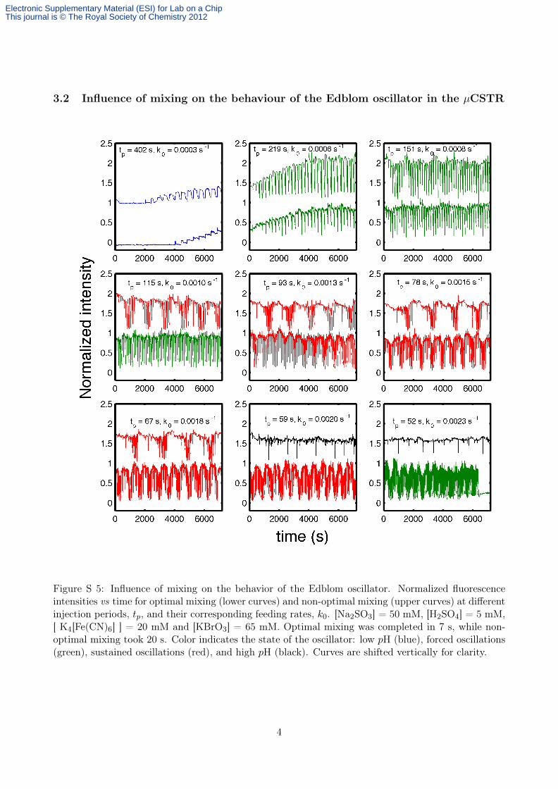
Figure S 5: Influence of mixing on the behavior of the Edblom oscillator. Normalized fluorescenceintensities vs time for optimal mixing (lower curves) and non-optimal mixing (upper curves) at differentinjection periods, tp, and their corresponding feeding rates, k0. [Na2SO3] = 50 mM, [H2SO4] = 5 mM,[ K4[Fe(CN)6] ] = 20 mM and [KBrO3] = 65 mM. Optimal mixing was completed in 7 s, while non-optimal mixing took 20 s. Color indicates the state of the oscillator: low pH (blue), forced oscillations(green), sustained oscillations (red), and high pH (black). Curves are shifted vertically for clarity.

4


4 pH of the bromate channel with and without purging

Figure S 6: Effect of the purging on the pH of the injected solution of KBrO3 65 mM. The pH is givenby the fluorescence of Oregon Green 10 µM. Purging was on (solid line) or off (dashed line). Theintensity was measured inside the injection channel, between valves 1 and 2.

5 Experimental pH vs time plots

In this section are displayed, in large format, the normalized fluorescence intensity vs time plotsrepresented in the phase diagram in Fig. 5A in the Main Text. The following conditions are commonto all graphs: 5 mM H2SO4, 20 mM K4[Fe(CN)6], and 65 mM KBrO3. The graphs are color-coded asin the Main Text: low pH (black), forced oscillations (green), sustained oscillations (red), and high pH(black).

5


Figure S 7: Experimental normalized average fluorescence intensity for different injection periods, tp,and their corresponding feeding rates, k0, when the concentration of injected Na2SO3 was 25 mM.

6



7



8



9


6 Simulations

6.1 Model of the Edblom oscillator

Edblom et al1 demonstrated that the main features of the oscillator studied in this work were describedwith the following set of reactions

BrO−3 + HSO−3k1→ HBrO2 + SO2−

4 k1 = 8× 10−2M−1s−1 (1)

HBrO2 + Br− + H+ k2→ 2HOBr k2 = 9.5× 106M−2s−1 (2)

HOBr + Br− + H+ k3→ Br2 + H2O k3 = 1.6× 1010M−2s−1 (3)

Br2 + H2Ok4→ HOBr + Br− + H+ k4 = 1.1× 101s−1 (4)

2HBrO2k5→ BrO−3 + HOBr + H+ k5 = 3× 103M−1s−1 (5)

Br2 + HSO−3 + H2Ok6→ 2Br− + SO2−

4 + 3H+ k6 = 1.0× 106M−1s−1 (6)

H+ + SO2−3

k7→ HSO−3 k7 = 5.0× 1010M−1s−1 (7)

HSO−3k8→ H+ + SO2−

3 k8 = 3× 103s−1 (8)BrO−3 + 2Fe(CN)4−6 + 3H+ = HBrO2 + 2Fe(CN)3−6 + H2O (9)

BrO−3 + Fe(CN)4−6 + H+ k9→ HBrO2 + Fe(CN)3−6 + H2O k9 = 3.2× 101M−2s−1, (10)

where (9) defines the stœchiometry of the oxydation of Fe(CN)4−6 and (10) accounts for the mechanismfrom which the rate is computed. The rates for reactions 1 to 9 are

r1 = k1[BrO−3 ][HSO−3 ] (11)r2 = k2[HBrO2][ Br−][ H+] (12)r3 = k3[HOBr][Br−][H+] (13)r4 = k4[Br2] (14)r5 = k5[HBrO2]2 (15)r6 = k6[Br2][HSO−3 ] (16)r7 = k7[H+][ SO2−

3 ] (17)r8 = k8[HSO−3 ] (18)r9 = k9[BrO−3 ][Fe(CN)4−6 ][ H+]. (19)

The differential equations describing the temporal evolution of the species involved in the Edblomoscillator in a CSTR are thus

1E. C. Edblom, Y. Luo, M. Orban, K. Kustin and I. R. Epstein, J. Phys. Chem., 1989, 93, 2722-2727.

10


d[Br−]dt

= −r2 − r3 + r4 + 2r6 − k0[Br−] (20)

d[Br2]dt

= r3 − r4 − r6 − k0[Br2] (21)

d[HOBr]dt

= 2r2 − r3 + r4 + r5 − k0[HOBr] (22)

d[HBrO2]dt

= r1 − r2 − 2r5 + r9 − k0[HBrO2] (23)

d[BrO−3 ]dt

= −r1 + r5 − r9 + k0

([KBrO3]IN − [ BrO−3 ]

)(24)

d[SO2−3 ]

dt= −r7 + r8 + k0

([Na2SO3]IN − [ SO2−

3 ])

(25)

d[HSO−3 ]dt

= −r1 − r6 + r7 − r8 − k0[HSO−3 ] (26)

d[Fe(CN)4−6 ]dt

= −2r9 + k0

([K4Fe(CN)6]

IN − [Fe(CN)4−6 ])

(27)

d[Fe(CN)3−6 ]dt

= 2r9 − k0[Fe(CN)3−6 ] (28)

d[H+]dt

= −r2 − r3 + r4 + r5 + 3r6 − r7 + r8 − 3r9 + r10 + k0

([H+]IN − [H+]

), (29)

where k0 is the feeding rate, [I]IN is the concentration of species I being injected in the CSTR. [H+]is being injected as H2SO4, an acid with pKa,1 = −3 and pKa,2 = 2. The lowest pH of the oscillatorbeing about 2, we can consider that H2SO4 exists in solution only as species HSO−4 and SO2−

4 . Ata given time, for a proton concentration in the reactor [H+], an injection of [H2SO4]IN results in aninjected concentration of protons given by

[H+]IN = [H2SO4]IN

(1 +

1(1 + [H+]/Ka,2)

). (30)

We consider here that the protonation equilibra of H2SO4 are infinitely fast compared with reactions1 to 9. We do neglect the contribution of protons coming from a remaining quantity of HSO−4 at lowpH that would liberate protons when the pH rises in the reactor.

Equations (20) to (29) take the form of Equation 1 in the Main Text, that we reproduce here forclarity,

dCi(t)dt

= fi (kj , Cl(t)) + k0

(CIN

i − Ci(t)). (31)

The system of equations (20) to (29) can be simulated in a macroscopic CSTR as is. In contrast, tosimulate these equations in a µCSTR we need to take into account the digital character of the injection.For each species i, (31) was rewritten as

dCi(t)dt

= χ(1−H)fi (kj , Cl(t)) +Hk0

tinj

(CIN

i − Ci(t)), (32)

where H is a function that takes into account the digital character of the injection. It is equal to 1during the injection phase, that lasted tinj = 5 s in our simulations, and equal to 0 otherwise. Note

11


that this implementation assumes perfect mixing as soon as the injection phase ends. χ is a couplingparameter that we have added to remove a divergence due to the sharp change in the derivativeintroduced by the discontinuous function H. After an injection, the concentrations of the differentspecies may change quite abruptly and make the computed derivative very large, thus introducing, forinstance, negative values of the concentrations. To smooth this effect, the contribution of fi (kj , Cl(t))to (32) was switched on linearly after an injection, with χ = t/tswicth, and tswitch = 10 s.

Differential equations were solved in Matlab using ode23s solver for stiff problems. It is a one-stepsolver that uses a modified Rosenbrock formula of order 2.

6.2 Comparison experiments/simulations in a closed reactor

The experimental and simulated phase diagram of the Edblom oscillator in the same conditions (5 mMH2SO4, 20 mM K4[Fe(CN)6], and 65 mM KBrO3), displayed in Figure 11, are significantly different.Several reasons can be invoked to explain this discrepacy: i) mixing in the experiments takes 7 s, whilein the simulations it is instantaneous, ii) injection and mixing are considered independent processes inthe simulations, but they are simultaneous, and coupled to spatial transport, in the experiments, iii)the high surface to volume ratio of the µCSTR is not taken into account in the simulations, notablythe evaporation of important intermediates such as Br2 through the porous walls of PDMS, and iv)the influence of the fluorescent dye is disregarded in the simulations. Instead of studying each ofthese processes in detail we decided to take a phenomenological description. To do so we performeda series of experiments, and the corresponding simulations, using the µCSTR as a closed reactor fordifferent concentrations of H2SO4 and Na2SO3. In these experiments the four reagents were injected50 consecutive times into the annular reactor and mixed to create a reproducible initial conditioncorresponding to 1/4 of the volume of the reactor for each injected solution. The injection valves wereclosed, mixing remained active and fluorescence was recorded. The results are displayed in Figure 12.For all the experiments the fluorescence intensity (the pH) stays high and stable until it abruptlydrops (within 30 s) and remains low. The time at which the fluorescence (pH) drops depends on[Na2SO3] and [H2SO4]. The behavior of the Edblom oscillator at 5 mM H2SO4 in a closed reactor issignificantly different for the experiments and the simulations. In contrast, results are similar when wecompare simulations and experiments at 10 and 5 mM H2SO4 respectively. We argue that increasingthe concentration of H2SO4 in the simulations to 10 mM phenomenologically takes into account thefactors evoked above that are not incroporated in the simulations. We thus compare, in the Figure 5of the Main Text, the experimental phase diagram at 5 mM H2SO4 with the simulated phase diagramat 10 mM H2SO4 .

12


Figure S 11: Experimental (top) and simulated (bottom) phase diagram of the Edblom oscillator inthe µCSTR for different Na2SO3 input concentrations and at different feeding rates k0 (and theircorresponding injection periods tp). Each square represents pH vs. time during a 2 h experiment.Time traces are colour-coded according to the observed steady state: low pH (blue), forced oscillations(green), sustained oscillations (red), and high pH (black). In contrast with Fig. 5 in the Main Text,here [H2SO4] = 5 mM both for the experiment and for the simulations. The remaining injectedconcentrations are K4[Fe(CN)6] 20 mM and KBrO3 65 mM.

13


Figure S 12: Normalized intensity (experiments, solid lines) or normalized pH (simulations, dashedlines) vs time after mixing in a closed reactor for different concentrations of Na2SO3 (25 mM, green,50 mM, blue, 75 mM, black, and 100 mM, magenta) and H2SO, and for 20 mM K4[Fe(CN)6] and 65mM KBrO3.

14


6.3 Simulated pH vs time plots

In this subsection are displayed, in large format, the normalized pH vs time plots represented in thephase diagram in Fig. 5B in the Main Text. The following conditions are common to all graphs:[H2SO4] = 10 mM, K4[Fe(CN)6] 20 mM and KBrO3. 65 mM. The graphs are color-coded as in theMain Text: low pH (black), forced oscillations (green), sustained oscillations (red), high pH (black).

Figure S 13: Simulated normalized average fluorescence intensity for different injection periods, tp, andtheir corresponding feeding rates, k0 when the concentration of injected Na2SO3 was 25 mM.

15



16



17



7 Attached files

7.1 Video of the Edblom oscillator in the µCSTR

A video showing two periods of the Edblom oscillator for 20 mM K4[Fe(CN)6], 65 mM KBrO3, 75 mMNa2SO3, and 5 mM H2SO4 being injected, with a period tp = 115 s, in the µCSTR and observed with10µM Oregon green under a fluorescence microscope is available for download.

18


Figure S 17: First frame of the attached video.

7.2 Matlab code for simulations

The Matlab code for the simulations described in section 6 is available for download. It is constitutedof the following functions:

function do_solve_Edblom_kinetics_for_several_input% Calls the solver plot_solutions_parameter_Edblom_kinetics for%different concentrations of sulfite and sulfuric acid

function plot_solutions_parameter_Edblom_kinetics(varargin)%Calls the ODE solver function solve_kinetics_with_parameters_CSTR_Edblom( pumpingPeriod(i),%fId ) for different values of pumpingPeriod. Then makes plots with the%results from that function. ’param’ and ’out’ are the principal%structures, with the parameters and the output values%If varargin > 0 the first one is the input sulfite conc and the second one%the input sulfuric acid conc

function [t y] = solve_kinetics_with_parameters_CSTR_Edblom(param, x0, iCondition)% This function implements the kinetic model for the pH oscillator in a CSTR described%in Edblom, JPhysChem 1989, Table 1%in a continuous or digital CSTR modeled through k0%Input is a structure param with the rate constants and the file id fId to write%results in a text file, x0 is a vector containing the initial conditions,%’iCondition’ is a counter for an experiment with different k0%OUPUT are vectors time ’t’ and solution of the%ODE ’y’ as well as the structure param with normalized rates sigmai

function param = create_parameter_struct_Edblom()% Initializes the structure ’param’ which stocks all the relevant parameters%set by the user to solve the ODEs

function out = create_output_struct_Edblom()% Initializes the structure ’out’ which stocks all the quantities%computed during the simulation

19


function jacob = edblom_jacobian(x, rate, H, chemCoupling, k0Comp)% Claculates the Jacobian matrix of the Edblom ODE system% written in function solve_kinetics_with_parameters_CSTR_Edblom% INPUT: ’x’ vector of concentrations, ’rate’ structure of rates% ’H’ equal to 0 or 1 depending on injection conditions, ’cte’% equal to 1 or 2 for digital or continuous injection,% ’k0Comp’ computed k0 value

function plot_Edblom_data(out, param)% Plots outputs from function plot_solutions_parameter_Edblom_kinetics% out and param are structures defined in that function

20


Documents

Lab on a Chip - C2N – Accueil reactors, called continuous stirred tank reactors (CSTR), have been instrumental for investigating the dynamics of out-of-equilibrium chemical processes,