Embed Size (px)
Citation preview
SIMULATION OF CONTINUOUS STIRRED TANK
REACTORS (CSTR’S) USING ORTHOGONAL
FUNCTIONS A THESIS SUBMITTED IN PARTIAL FULFILLMENT OF THE
REQUIREMENTS FOR THE AWARD OF THE DEGREE OF
Master of Technology
In
Chemical Engineering
Department of Chemical Engineering
By
KAMESWARI MANI PRIYANKA NEMANI
Roll No: 213CH1125
Under the Guidance of
Prof. Madhusree Kundu
Department of Chemical Engineering
National Institute Technology, Rourkela-769008
ii
NATIONAL INSTITUTE OF TECHNOLOGY
ROURKELA
CERTIFICATE
This is to certify that the project entitled “SIMULATION OF CONTINUOUS STIRRED
TANK REACTORS (CSTR’s) USING ORTHOGONAL FUNCTIONS” submitted by
Kameswari Mani Priyanka Nemani (213CH1125) in partial fulfilment of the requirements
for the award of Master of Technology degree in Chemical Engineering, Department of
Chemical Engineering at National Institute of Technology, Rourkela is an authentic work
carried out by her under my supervision and guidance.
To the best of my knowledge the matter embodied in this thesis has not been submitted to any
other university/Institute for the award of any Degree.
Date: Prof. Madhusree Kundu
Place: Rourkela Department of Chemical Engineering
NIT Rourkela
iii
ACKNOWLEDGEMENT
On the submission of my thesis entitled “SIMULATION OF CONTINUOUS STIRRED
TANK REACTORS (CSTR’s) USING ORTHOGONAL FUNCTIONS” I would like to
express my most sincere gratitude to Dr. Madhusree Kundu, my professor and thesis
advisor, for her continuous guidance, encouragement and patience during the course of my
project .Her direct contributions helped me in the completion of the thesis. I would like to
thank the head of the department Prof.P.Rath for supporting me with all the necessary
equipment and for giving such a supportive advisor.
And also thank D.Seshu Kumar, Research Scholar for helping me appreciate the underlying
mathematical aspects of this project and Sujeevan Kumar Agir, Research scholar. Thank you
to all my professors and technicians in the Department of Chemical Engineering.
I would like to thank all others who have consistently encouraged and gave me moral support,
without whose help it would be difficult to finish this project.
I would like to thank my parents and friends for their consistent support throughout.
1
ABSTRACT
Over the centuries, several numerical methods have been developed to approximate the solution
of mathematical problems that are difficult to be solved by analytical methods. These numerical
techniques succeeded in attaining a solution that is close enough to the exact solution with
minimum errors and maximum stability. However, there may be the development of several
other numerical methods which can be robust and efficient than the existing methods.My
proposed research work is about the application of one such method-Orthogonal functions.
Orthogonal functions can be broadly classified in to three families; namely, the piecewise
constant, polynomial, and sine-cosine family. Walsh function and block pulse function belong to
the piecewise constant family. So far orthogonal functions have been used in the optimal control,
solving integro-differential equations, trajectory problems and so on. However, orthogonal
functions have not been applied to chemical systems and processes. Hence my work is
emphasised on simulating reactors using orthogonal functions; mainly block pulse functions and
triangular functions.
The continuous stirring tank reactors (CSTR’s) are widely used in the chemical industries. Hence
the reactions in a CSTR are modelled by a set of differential equations which are discretised to a
set of algebraic equations by orthogonal functions. Previously many numerical methods such as
Runge-Kutta method, Euler method have successfully converted the set of differential equations
into a set of algebraic equations. But the orthogonality of the functions has never been used for
discretisation. Here orthogonal functions simulate chemical reactors using the principle of
orthogonality (two functions are said to be orthogonal if the dot product of the approximating
vectors is zero). Block-pulse functions have been used to obtain the dynamics of concentration
and temperature of the continuous stirring tank reactors (CSTR’s). Further a recurrence
relationship developed using block-pulse functions and triangular functions have been used in
solving linear and non-linear system of differential equations. The major importance of
orthogonal functions lies in its application to optimal control to systems. A recursive algorithm
developed using block pulse functions has been applied to a linear control problem to determine
the states and optimality criterion.
Keywords: Orthogonal functions, Block pulse functions, Triangular functions, system
identification and optimal control.
2
TABLE OF CONTENTS
Abstract 1
Table of contents 2
List of tables 4
List of figures 5
CHAPTER-1 INTRODUCTION TO NUMERICAL TECHNIQUES
1.1 Numerical Analysis 9
1.1.1 Numerical methods for ODE’s 10
1.1.2 Euler Method 11
1.2 Orthogonal Functions 12
1.2.1 Block Pulse Functions 13
1.2.2 Triangular Functions 18
1.2.3 Optimal Control with OF 18
1.3 Objective 18
1.4 Scope 18
1.5 Thesis Organization 19
CHAPTER-2 LITERATURE SURVEY
2.1 Literature Survey 21
CHAPTER-3 SIMULATION OF LINEAR AND NON-LINEAR
SYSTEMS USING OPERATIONAL MATRICES OF BLOCK PULSE
FUNCTIONS
3.1 Linear Systems 26
3.2 Simulation of Linear Systems 27
3.2.1 Results and Discussions 47
3
3.3 Non-Linear Systems 48
3.3.1 Differences between Linear and Non Linear Systems 49
3.3.2 Definition of Linear and Non-Linear Systems 49
3.3.3 Non-Linear Differential Equations 51
3.4 Simulation of Non-Linear Systems 52
3.4.1 Results and Discussions 56
CHAPTER-4 SIMULATION OF LINEAR AND NON-LINEAR
SYSTEMS VIA ORTHOGONAL FUNCTIONS BY RECURRENCE
RELATION
4.1 Recurrence relation using Triangular Functions for Linear Systems 58
4.2 Simulation of Linear systems via Recurrence Relation 61
4.2.1 Results and Discussions 67
4.3 Simulation of Non-Linear systems via Recurrence Relation 67
4.3.1 Results and Discussions 73
CHAPTER-5 OPTIMAL CONTROL OF CSTR’S USING
ORTHOGONAL FUNCTIONS
5.1 Optimal Control of Systems 75
5.1.1 Analysis of Linear Control Systems Incorporating Observers 77
5.1.2 Results and Discussions 81
CHAPTER-6 CONCLUSION AND FUTURE SCOPE
6.1 Conclusion 83
6.2 Future Scope 83
REFERENCES 84
4
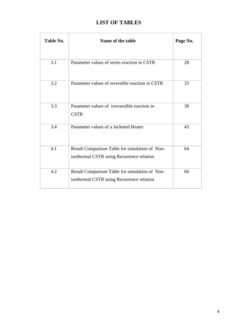
LIST OF TABLES
Table No.
Name of the table
Page No.
3.1
Parameter values of series reaction in CSTR
28
3.2
Parameter values of reversible reaction in CSTR
33
3.3
Parameter values of irreversible reaction in
CSTR
38
3.4
Parameter values of a Jacketed Heater
43
4.1
Result Comparison Table for simulation of Non-
isothermal CSTR using Recurrence relation
64
4.2
Result Comparison Table for simulation of Non-
isothermal CSTR using Recurrence relation
66
5
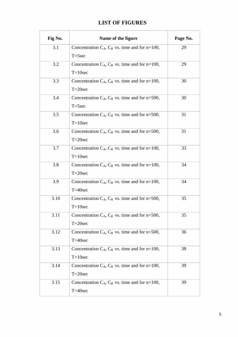
LIST OF FIGURES
Fig No.
Name of the figure
Page No.
3.1
Concentration CA, CR vs. time and for n=100,
T=5sec
29
3.2
Concentration CA, CR vs. time and for n=100,
T=10sec
29
3.3
Concentration CA, CR vs. time and for n=100,
T=20sec
30
3.4
Concentration CA, CR vs. time and for n=500,
T=5sec
30
3.5
Concentration CA, CR vs. time and for n=500,
T=10sec
31
3.6
Concentration CA, CR vs. time and for n=500,
T=20sec
31
3.7
Concentration CA, CR vs. time and for n=100,
T=10sec
33
3.8
Concentration CA, CR vs. time and for n=100,
T=20sec
34
3.9
Concentration CA, CR vs. time and for n=100,
T=40sec
34
3.10
Concentration CA, CR vs. time and for n=500,
T=10sec
35
3.11
Concentration CA, CR vs. time and for n=500,
T=20sec
35
3.12
Concentration CA, CR vs. time and for n=500,
T=40sec
36
3.13
Concentration CA, CR vs. time and for n=100,
T=10sec
38
3.14
Concentration CA, CR vs. time and for n=100,
T=20sec
39
3.15
Concentration CA, CR vs. time and for n=100,
T=40sec
39
6
3.16
Concentration CA, CR vs. time and for n=500,
T=10sec
40
3.17
Concentration CA, CR vs. time and for n=500,
T=20sec
40
3.18
Concentration CA, CR vs. time and for n=500,
T=40sec
41
3.19
Temperature T, Tj vs. time and for n=100,
T=10sec
44
3.20
Temperature T, Tj vs. time and for n=100,
T=20sec
44
3.21
Temperature T, Tj vs. time and for n=100,
T=40sec
45
3.22
Temperature T, Tj vs. time and for n=500,
T=10sec
45
3.23
Temperature T, Tj vs. time and for n=500,
T=20sec
46
3.24
Temperature T, Tj vs. time and for n=500,
T=40sec
46
3.25
Concentration CG, CX and CI vs. time and for
n=100, T=100sec
54
3.26
Concentration CG, CX and CI vs. time and for
n=500, T=500sec
55
3.27
Concentration CG, CX and CI vs. time and for
n=1000, T=1000sec
55
4.1
Concentration CA, CP vs. time and for n=10,
T=10sec
62
4.2
Concentration CA, CP vs. time and for n=50,
T=50sec
63
4.3
Concentration CA, CP vs. time and for n=100,
T=100sec
63
7
4.4
Concentration CA, CP vs. time and for n=100,
T=10sec
65
4.5
Concentration CA, CP vs. time and for n=100, T=20sec
65
4.6
Concentration CA, CP vs. time and for n=100, T=30sec
66
4.7
Concentration CA, T and Tj vs. time and for m=2, T=50sec
69
4.8
Concentration CA, T and Tj vs. time and for m=5, T=50sec
70
4.9
Concentration CA, T and Tj vs. time and for m=2, T=100sec
70
4.10
Concentration CA, T and Tj vs. time and for m=1, T=500sec
71
4.11
Concentration CG, CX and CI vs. time and for
m=2, T=10sec
72
4.12
Concentration CG, CX and CI vs. time and for
m=2, T=20sec
72
4.13
Concentration CG, CX and CI vs. time and for
m=2, T=20sec
73
5.1 Error versus time, t=10sec,m=4 79
5.2 State Variables versus time, t=10sec,m=4 80
5.3 State Variables versus times, t=10sec, m=9 80
5.4 State Variables versus time, t=10sec, m=9 81
8
CHAPTER-1
INTRODUCTION TO NOVEL NUMERICAL
TECHNIQUES APPLIED IN PROCESS
SIMULATION AND CONTROL

9
1.1 NUMERICAL ANALYSIS
Numerical analysis is useful in practical mathematical calculations obtaining approximate
solutions with a reasonable bound of errors. The Babylonian tablet that was the earliest
mathematical writings approximated √ (2) the length of the diagonal of a unit square.
Numerical analysis is applicable to all fields of engineering and physical sciences. They were
used in solving System of Equations, Eigenvalues and Singular value problems, Numerical
Integration, Ordinary and Partial Differential Equations. The overall goal of the numerical
analysis is the design and analysis of techniques to approximate solutions of difficult
problems accurately. A numerical method not only develops methods but also analyses them
by three central concepts: convergence, stability, order. It works with a wide variety of
problems such as:
It makes weather prediction feasible.
Computing the trajectory of a spacecraft requires an accurate numerical solution of a
system of Ordinary Differential equations (ODE’s).
Car companies can improve the crash safety of their vehicles using computer
simulations of car crashes, which involves solving partial differential equations.
Insurance companies use numerical analysis for actuarial analysis.
Computation of solution to a problem in finite number of steps is possible by direct methods
giving precise answers. Examples of direct methods include Gaussian elimination, QR
factorization for solving linear equations and simplex method for linear programming.
Indirect methods take infinite number of steps to produce output to a problem. It starts with an
initial guess forming successive approximation and converges to the exact solution with a
limit. It also includes a convergence test to decide the accuracy of the solution once it has
been obtained. Examples of such methods are Newton-Raphson method, Bisection method
and Jacobi iteration. Iterative methods otherwise called as indirect methods are more common
than the direct methods.
The important part of the numerical analysis deals with a study of errors, which comprises of
round-off errors, truncations errors, discretization errors. Round-off errors arise due to non-
representation of all real numbers exactly on a machine with finite memory. Truncation errors
occur due to termination of an iterative method or a mathematical procedure, which results in
10
approximate solution differing from the exact solution. Discretization error is caused when the
discretized problem solution does not coincide with that of the continuous problem.
The other important part of the numerical analysis is stability, i.e. a procedure is said to be
numerically stable if the error does not grow to a large extent during calculation, which means
problem should be well conditioned. When the problem was well conditioned, the solution
changes by a small amount for a small change introduced in the input data. However, an ill-
conditioned problem exhibits significant deviation for small changes in data. Thus, the art of
numerical analysis is to find a stable algorithm for solving a well-defined mathematical
problem.
Most of the chemical reactions we come across in the industry are systems to which certain
inputs are given and outputs are expected either in terms of mass compositions, temperatures,
and pressures. We deal with non-ideal systems in which inputs get accumulated within the
reacting system as time proceeds. Thus, unlike the ideal system for which rate of input is
equal to rate of output, non-ideal systems have accumulation term equal to the difference
between the inputs and outputs. When a reaction occurs, reaction rate term gets included. All
these terms put together in mass balance equation and applying limits gives differential
equations. Therefore, industrial reacting systems precisely have differential equations to be
modelled. In order to analyse the real reactor behaviour, the proposed methods are to be
applied to these model equations (set of differential equation).Thus the proposed work focuses
on simulating differential equations within a reactor (CSTR).
1.1.1 Numerical Methods for Ordinary Differential Equations
Many differential equations cannot be solved by symbolic computation and hence practically
needs to be approximated to the exact solution. Thus, algorithms which can handle ordinary
differential equations are developed and used. Ordinary differential equations occur in many
disciplines such as in physics, biology, chemistry, economics and engineering. To obtain the
solution of some partial differential equations, they are converted to ODE’s and then solved.
Numerical methods for initial value problems (IVP’s) differ from that of boundary values
problems (BVP’s) which require a different set of tools. In a BVP, value or component of the
unknown variable is defined at more than one point unlike in the IVP, which defines an
unknown variable at the initial point of the system. Hence, BVP requires separate methods.

11
For solving first order initial value problems, methods are categorized into two types: linear
multistep methods and Runge-Kutta methods.
A further classification includes implicit and explicit methods. Implicit linear multistep
methods are the Adams-Moulton method and backward differentiation method (BDF)
whereas implicit Runge-Kutta methods include diagonally RK method, singly diagonally
implicit RK method and Gauss-Radau method. Explicit linear multistep methods are Adam-
Bashforth method and any Runge-Kutta method with lower diagonal Butcher tableau is
explicit. The rule of thumb is that for stiff differential equations implicit schemes must be
used and for non-stiff differential equations explicit methods can be used.
1.1.2 Euler Method
Euler method is an SN-order numerical procedure for solving ODE of IVP. It is regarded as
the primary explicit method for numerical integration of ODE’s and is the simplest of all
Runge-Kutta methods. Because it is a first-order method, the local error is proportional to the
square of step size while the global error is proportional to step size. Euler method forms the
basis for all sophisticated methods.
Forward Euler Method:-The forward Euler method is an explicit method which means a
new value 𝒚𝒏+𝟏 is defined in terms of known 𝒚𝒏
𝒚′(𝒕) =𝒚(𝒕 + 𝒉) − 𝒚(𝒕)
𝒉… … … … … … … … … … … … … … … … … … … … … … … … … … … (𝟏. 𝟏)
𝒚(𝒕 + 𝒉) = 𝒚(𝒕) + 𝒉𝒚′(𝒕) … … … … … … … … … … … … … … … … … … … … … … … … … … (𝟏. 𝟐)
𝒚(𝒕 + 𝒉) = 𝒚(𝒕) + 𝒉𝒇(𝒕, 𝒚(𝒕)) … … … … … … … … … … … … … … … … … … … … … … … … (𝟏. 𝟑)
𝒚𝒏+𝟏 = 𝒚𝒏 + 𝒉𝒇(𝒕𝒏, 𝒚𝒏) … … … … … … … … … … … … … … … … … … … … … … … … … … … (𝟏. 𝟒)
Backward Euler method:-The backward Euler method, unlike the forward Euler method, is
an implicit method in which the equation has to be solved to find out 𝒚𝒏+𝟏 , hence Newton-
Raphson method is used. One disadvantage of an implicit method like Backward Euler
method is the time for computation that is very high. However, the advantage is that implicit
methods are more stable for solving stiff differential equations, and a large step size can be
used.
12
𝒚′(𝒕) =𝒚(𝒕) − 𝒚(𝒕 − 𝒉)
𝒉… … … … … … … … … … … … … … … … … … … … … . … … … … … . (𝟏. 𝟓)
𝒚𝒏+𝟏 = 𝒚𝒏 + 𝒉𝒇(𝒕𝒏+𝟏, 𝒚𝒏+𝟏) … … … … … … … … … … … … … … … … … … … … … … … … … (𝟏. 𝟔)
The Euler method is often not very accurate as it considers only first order equations ignoring
higher order equations. In such multistep methods, one gets to use the previously computed
value 𝒚𝒏 to determine new value 𝒚𝒏+𝟏 . In case if more points are used in the interval, it leads
to Runge-Kutta method.
1.2 ORTHOGONAL FUNCTIONS
In mathematics, two functions 𝑓 and 𝑔 are called orthogonal if their inner product (𝑓, 𝑔) is
zero for f≠g. A typical definition of inner product is∫ 𝑓 ∗ (𝑥)𝑔(𝑥), where 𝑓 ∗ (𝑥)the complex
conjugate of function is‘𝑓’. The inner product of f and g can be roughly approximated as the
dot product between two vectors𝑓, 𝑔. Thus, two functions are orthogonal if their
approximating vectors are perpendicular. Orthogonality of functions is a generalization
concept of orthogonalization of vectors. Suppose we define 𝑉 to be set of variables on which
functions 𝑓 and 𝑔 operate then if 𝑉 = {𝑥}, 𝑥 is the only parameter to 𝑓 and 𝑔, thus there is
one parameter; hence one integral sign is required to determine orthogonality.
Orthogonal functions can be broadly classified in to three families; namely, the piecewise
constant, polynomial, and sine-cosine family. Harr functions, Block pulse functions, Delay-
unit step functions, Slant functions, Triangular functions, Rademacher functions, Walsh
function and block pulse function belong to the piecewise constant family while Chebyshev
polynomial of first and second kind, Laguerre polynomial, Hermite polynomials, Jacobi
polynomials together with their special cases the Gegenbauer polynomials, and Legendre
polynomials belong to the polynomial family. Functions at any time can be synthesized using
a set of orthogonal functions with a tolerable degree of accuracy. An orthogonal polynomial
sequence is a family of polynomials such that any two different polynomials in the sequence
are orthogonal to each other under some inner product.
The sine-cosine functions or orthogonal polynomials can represent a continuous function,
however, becomes unsatisfactory for representing functions with discontinuities, jumps or
dead-time. For representing such functions, piece-wise constant orthogonal functions such as
Walsh functions or block pulse functions can be used. Each class of orthogonal functions
13
forms a basis for series expansion of a square integrable function, OFs’ are commonly called
as basis functions.
Orthogonal functions are used to construct operational matrices for solving, identification and
optimization problems of dynamic systems. They help in dealing with various problems of
dynamic systems as it reduces to those of solving algebraic equations. By using this approach,
differential equations are converted into integral equations through integration, approximating
various signals involved in the equation by truncated orthogonal functions and using
operational matrices of integration to eliminate integral operation.
1.2.1 Block-pulse Functions
An orthogonal block-pulse function has been used to obtain the dynamics of concentration
and temperature of the continuous stirring tank reactors. The operational matrix, P of the
block-pulse functions eliminates integration operation and hence simplifies the system of state
equations into a set of algebraic equations. The algorithm using BPF has been developed in
the MATLAB platform. The idea is to present the states and outputs in terms of these block-
pulse functions. The present method is advantageous over the existing methods like Runge-
Kutta, Laplace transformations, State-space approach in terms of its simplicity in operation
and accuracy.
Operational Matrix Derivation
An m-set of BPF is defined as follows:
𝜱𝒊(𝒕) = {𝟏, 𝒊𝒉 ≤ 𝒕 ≤ (𝒊 + 𝟏)𝒉
𝟎, 𝒐𝒕𝒉𝒆𝒓𝒘𝒊𝒔𝒆, (1.7)
Where 𝑖 = 1,2, . . . . . . . , 𝑚 − 1 with positive integer values for m, and h=T/m, and m are
arbitrary positive integers. There are some properties for BPFs, e.g. disjointness,
orthogonality, and completeness.
Disjointness: - The block-pulse functions are disjoint with each other; i.e.,
𝜱𝒊(𝒕)𝜱𝒋(𝒕) = {𝜱𝒊(𝒕), 𝒊 = 𝒋,
𝟎, 𝒊 ≠ 𝒋 (1.8)
Where 𝑖, 𝑗 = 0, . . . . . . , 𝑚 − 1.
Orthogonality: - The block-pulse functions are orthogonal with each other i.e.,
14
∫ 𝜱𝒊(𝒕)𝜱𝒋(𝒕)𝒅𝒕 = {𝒉, 𝒊 = 𝒋,
𝟎, 𝒐𝒕𝒉𝒆𝒓𝒘𝒊𝒔𝒆 (1.9)
In the region of 𝑡 ∈ [0, 𝑇 ), where 𝑖, 𝑗 = 1, 2, . . . . . . . , 𝑚 − 1. This property is obtained from
the disjointness property.
Completeness:-
∫ 𝒇𝟐∞
𝟎(𝒕)𝒅𝒕 = ∑ 𝒇𝟐∞
𝟎 ║𝜱𝒊(𝒕)║𝟐
… … … … … … … … … … … … … … … … … … … … … … … . (𝟏. 𝟏𝟎)
Where,
𝒇𝒊 = 𝟏/𝒉 ∗ (∫ 𝒇(𝒕)𝜱𝒊(𝒕))𝒅𝒕𝟏
𝟎
… … … … … … … … … … … … … … … … … … . … … … … . … (𝟏. 𝟏𝟏)
The set of BPFs may be written as an m-vector (t):
𝜱(𝒕)𝜱𝑻(𝒕) = 𝟏, … … … … … … … … … … … … … … … … . . … … … … (𝟏. 𝟏𝟐)
Where t ∈ [0, 1). From the above representation and disjointness property, it follows:
𝜱(𝒕) = [𝜱𝟎(𝒕), . . . . . . . , 𝜱𝒎−𝟏(𝒕)]𝑻
… … … … … … … … … … … … . … . … (𝟏. 𝟏𝟑)
𝜱 (𝒕)𝜱𝑻(𝒕) = [𝜱𝟎(𝒕) ⋯ 𝟎
⋮ ⋱ ⋮𝟎 ⋯ 𝜱𝒎−𝟏(𝒕)
] … … … … … … … . . . … … … … … … . . … … … . … (𝟏. 𝟏𝟒)
𝜱(𝒕)𝜱𝑻(𝒕)𝑽 = �̃�𝜱(𝒕) … … . … … … … . . … … … … … . . . . (𝟏. 𝟏𝟓)
Where V is an m-vector and 𝑉 = 𝑑𝑖𝑎𝑔(𝑉 ). moreover, it can be clearly concluded that for
every m x m matrix A:
15
𝜱(𝒕)𝑻𝑨𝜱(𝒕) = �̂�𝑻𝜱(𝒕) … . . … … … … … … … . … … … . . . (𝟏. 𝟏𝟔)
Where A is an m-vector with elements equal to the diagonal entries of matrix A.
Functions approximation:-
A function 𝑓(𝑡), 𝐿€([0,1)) may be expanded by the BPFs as:
𝑭(𝒕) = ∑ 𝑭𝒊𝜱𝒊(𝒕) = 𝑭𝑻𝜱(𝒕) = 𝜱𝑻(𝒕)𝑭 … … … … . … … . . … . . … . (𝟏. 𝟏𝟕)
where F is a m-vector given by
𝑭 = [𝒇𝟎, . . . . . . . . 𝒇𝒎−𝟏]𝑻
… … … … … … … … … … … … … … . . . . . (𝟏. 𝟏𝟐)
𝜱(𝒕) = [𝜱𝟏(𝒕) , 𝜱𝟐(𝒕), . . . . . . . . , 𝜱𝒎−𝟏(𝒕) ]𝑻
… … … … … … … … … … … … … … … … … … . . . (𝟏. 𝟏𝟑)
The block-pulse 𝑐𝑜𝑒𝑓𝑓𝑖𝑐𝑖𝑒𝑛𝑡𝑠 𝑓i are obtained as:
𝒇𝒊 =𝟏
𝒉∫ 𝒇(𝒕)𝜱𝒊(𝒕) 𝒅𝒕 … … … … … … … … … … … … … … . . . . . (𝟏. 𝟏𝟒)
such that error between f(t), and its block-pulse expansion in the region of t ∈ [0,1)
𝜺 = ∫ (𝒇 − ∑𝒇𝒊𝜱𝒊(𝒕))𝟐𝒅𝒕𝒎−𝟏
𝒊=𝟎
… … … … … … … … … … . … … … . (𝟏. 𝟏𝟓)
𝒌(𝒙, 𝒕) = 𝜱𝑻(𝒙)𝑲𝜱(𝒕) … … … … … … … … … … . … … … . … … (𝟏. 𝟏𝟔)
𝒌𝒊𝒋 = 𝒎𝟏𝒎𝟐 ∬ 𝒌(𝒙, 𝒕)𝜱𝒊(𝒙)𝜱𝒋(𝒕)𝒅𝒙𝒅𝒕 … … … … … . . … … . . … … … … … (𝟏. 𝟏𝟕)

16
Operational matrix Integration:-
We compute ∫ 𝜱𝒊(ح)𝒅ح𝒕
𝟎 as
∫ 𝜱𝒊(ح)𝒅ح𝒕
𝟎= {
𝟎, 𝒕 ≤ 𝒊𝒉𝒕 − 𝒊𝒉, 𝒊𝒉 ≤ 𝒕 ≤ (𝒊 + 𝟏)𝒉
𝒉, (𝒊 + 𝟏)𝒉 ≤ 𝒕 ≤ 𝟏 (1.18)
Then the above expression can be written as
∫ 𝜱𝒊(ح) 𝒅ح = (𝒕 − 𝒊𝒉)𝜱𝒊(𝒕) + 𝒉 ∑ 𝜱𝒋(𝒕)
𝒕
𝟎
… … … … … … … … … … . … . . . . (𝟏. 𝟏𝟗)
we have
𝑿 =𝟏
𝟐𝒉( ∑ [((𝒊 + 𝟏)𝒉)
𝟐− (𝒊𝒉)𝟐] 𝜱𝒊(𝒕)
𝒎−𝟏
𝒊−𝟏
) … … … … … … … … … . …. (𝟏. 𝟐𝟎)
By using orthogonal property, for0 ≤ 𝑖 ≤ 𝑚 , we have
∫ 𝜱𝒊 (ح) 𝒅 ح
𝒕
𝟎
= 𝟏/𝟐𝒉( ∑ [((𝒋 + 𝟏)𝒉)𝟐 − (𝒋𝒉)𝟐])𝜱𝒋(𝒕)𝜱𝒊(𝒕)
𝒎−𝟏
𝒋=𝟎
− (𝒊𝒉)𝜱𝒊(𝒕) + 𝒉∑𝜱𝒊(𝒕)
= 𝟏/𝟐𝒉[((𝒊 + 𝟏)𝒉)𝟐 − (𝒊𝒉)𝟐]𝜱𝒊((𝒕) − (𝒊𝒉)𝜱𝒊((𝒕) + 𝒉 ∑ 𝜱𝒊(𝒕)
=𝒉/𝟐𝜱𝒊 + 𝒉 ∑ 𝜱𝒋(𝒕)
… . … … … … … … … … … … … … … … … … … … … . … . . … … (𝟏. 𝟐𝟏)
The integration of the vector 𝛷(𝑡) may be obtained as:
∫ 𝜱(ح) 𝒅ح = 𝑷 𝜱(𝒕) … … … … … … … … … … … … … … … … … (𝟏. 𝟐𝟐)
Where P is called operational matrix of integration which can be represented by
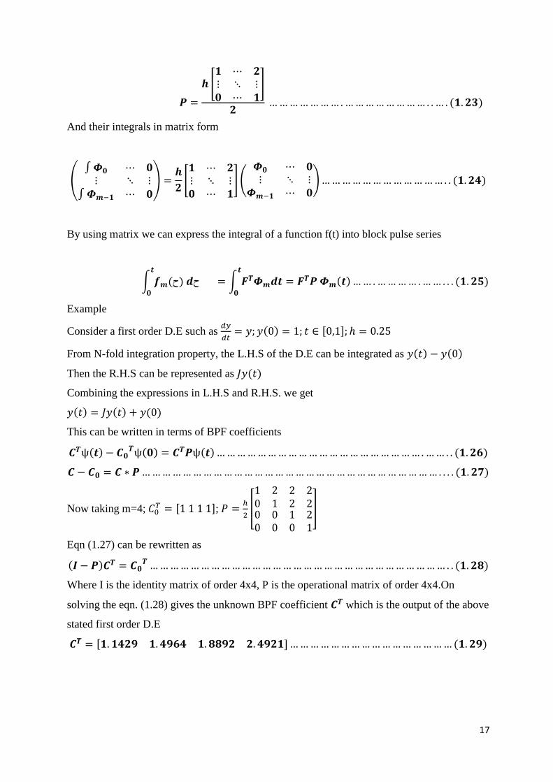
17
𝑷 =
𝒉 [𝟏 ⋯ 𝟐⋮ ⋱ ⋮𝟎 ⋯ 𝟏
]
𝟐 … … … … … … … . … … … … … … … … . . … . (𝟏. 𝟐𝟑)
And their integrals in matrix form
(∫ 𝜱𝟎 ⋯ 𝟎
⋮ ⋱ ⋮∫ 𝜱𝒎−𝟏 ⋯ 𝟎
) =𝒉
𝟐[𝟏 ⋯ 𝟐⋮ ⋱ ⋮𝟎 ⋯ 𝟏
] (𝜱𝟎 ⋯ 𝟎
⋮ ⋱ ⋮𝜱𝒎−𝟏 ⋯ 𝟎
) … … … … … … … … … … … … . . (𝟏. 𝟐𝟒)
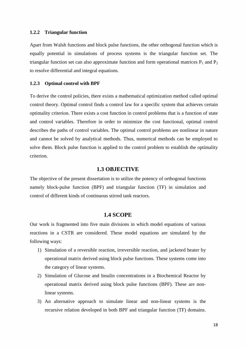
By using matrix we can express the integral of a function f(t) into block pulse series
∫ 𝒇𝒎(ح) 𝒅ح𝒕
𝟎
= ∫ 𝑭𝑻𝜱𝒎𝒅𝒕𝒕
𝟎
= 𝑭𝑻𝑷 𝜱𝒎(𝒕) … … . … … … … . … … . . . (𝟏. 𝟐𝟓)
Example
Consider a first order D.E such as 𝑑𝑦
𝑑𝑡= 𝑦; 𝑦(0) = 1; 𝑡 ∈ [0,1]; ℎ = 0.25
From N-fold integration property, the L.H.S of the D.E can be integrated as 𝑦(𝑡) − 𝑦(0)
Then the R.H.S can be represented as 𝐽𝑦(𝑡)
Combining the expressions in L.H.S and R.H.S. we get
𝑦(𝑡) = 𝐽𝑦(𝑡) + 𝑦(0)
This can be written in terms of BPF coefficients
𝑪𝑻ѱ(𝒕) − 𝑪𝟎𝑻ѱ(𝟎) = 𝑪𝑻𝑷ѱ(𝒕) … … … … … … … … … … … … … … … … … … … … . … … . . (𝟏. 𝟐𝟔)
𝑪 − 𝑪𝟎 = 𝑪 ∗ 𝑷 … … … … … … … … … … … … … … … … … … … … … … … … … … … … … . . . . (𝟏. 𝟐𝟕)
Now taking m=4; 𝐶0𝑇 = [1 1 1 1]; 𝑃 =
ℎ
2[
1 20 1
2 22 2
0 00 0
1 20 1
]
Eqn (1.27) can be rewritten as
(𝑰 − 𝑷)𝑪𝑻 = 𝑪𝟎𝑻 … … … … … … … … … … … … … … … … … … … … … … … … … … … … … . . (𝟏. 𝟐𝟖)
Where I is the identity matrix of order 4x4, P is the operational matrix of order 4x4.On
solving the eqn. (1.28) gives the unknown BPF coefficient 𝑪𝑻 which is the output of the above
stated first order D.E
𝑪𝑻 = [𝟏. 𝟏𝟒𝟐𝟗 𝟏. 𝟒𝟗𝟔𝟒 𝟏. 𝟖𝟖𝟗𝟐 𝟐. 𝟒𝟗𝟐𝟏] … … … … … … … … … … … … … … … … (𝟏. 𝟐𝟗)
18
1.2.2 Triangular function
Apart from Walsh functions and block pulse functions, the other orthogonal function which is
equally potential in simulations of process systems is the triangular function set. The
triangular function set can also approximate function and form operational matrices P1 and P2
to resolve differential and integral equations.
1.2.3 Optimal control with BPF
To derive the control policies, there exists a mathematical optimization method called optimal
control theory. Optimal control finds a control law for a specific system that achieves certain
optimality criterion. There exists a cost function in control problems that is a function of state
and control variables. Therefore in order to minimize the cost functional, optimal control
describes the paths of control variables. The optimal control problems are nonlinear in nature
and cannot be solved by analytical methods. Thus, numerical methods can be employed to
solve them. Block pulse function is applied to the control problem to establish the optimality
criterion.
1.3 OBJECTIVE
The objective of the present dissertation is to utilize the potency of orthogonal functions
namely block-pulse function (BPF) and triangular function (TF) in simulation and
control of different kinds of continuous stirred tank reactors.
1.4 SCOPE
Our work is fragmented into five main divisions in which model equations of various
reactions in a CSTR are considered. These model equations are simulated by the
following ways:
1) Simulation of a reversible reaction, irreversible reaction, and jacketed heater by
operational matrix derived using block pulse functions. These systems come into
the category of linear systems.
2) Simulation of Glucose and Insulin concentrations in a Biochemical Reactor by
operational matrix derived using block pulse functions (BPF). These are non-
linear systems.
3) An alternative approach to simulate linear and non-linear systems is the
recursive relation developed in both BPF and triangular function (TF) domains.
19
The recurrence relation in both domains is applied to two systems of irreversible
reactions.
4) Recurrence relation in BPF domain is applied to two non-linear systems:
Biochemical Reactor and Non-isothermal CSTR.
5) Optimal Control of CSTR’s using block-pulse functions.
1.5 THESIS ORGANIZATION
The thesis consists of six chapters in all .They are
Chapter 1: Introduction of numerical techniques
Chapter 2: Literature survey; in this chapter the details of other significant works done on the
applicability of orthogonal functions are presented.
Chapter 3: Simulation of linear and non-linear systems using operational matrices of block
pulse functions; the output variables are determined by converting model equations into a
system of linear algebraic equations with the help of operational matrix and this technique
includes no direct integration.
Chapter 4: Simulation of linear and non-linear systems via orthogonal functions by
recurrence relation; the output variables are determined by using the recurrence algorithm
developed from block pulse functions. The model equations are expressed in state-space
model and the matrices are substituted in recurrence relation which gives the output variables
i.e. the dynamics of the system can be established.
Chapter 5: Optimal control of CSTR’s using block pulse functions; this chapter deals with the
analysis of linear optimal control by incorporating observers. The error vector, state vector
and input vector are determined using the optimal control law and recurrence algorithm using
block pulse functions.
Chapter 6: Conclusions and Future Scope; in this chapter the extensions of the work and the
conclusions of present work are presented.

20
CHAPTER-2
LITERATURE SURVEY
21
LITERATURE SURVEY
A Substantial amount of research work has been carried out globally on the application of
orthogonal functions to various fields of engineering. These intensive studies laid a foundation
stone for the application of orthogonal functions to chemical engineering. Here are a list of
works briefly detailing their scope and magnitude of orthogonal functions.
The Legendre polynomial originated in determining the force of attraction exerted by solids of
revolution and their orthogonal properties were established by A. M. Legendre during 1784-
1790. Piecewise constant OF’s basis functions having constant functional values within any
subinterval of time period. Block pulse function is a complete OF, which provides elegant
solution to the areas of parameter estimation, analysis and control. Substantial amount of
research work has been carried out globally on the application of orthogonal functions to
various fields of engineering. These intensive researches laid foundation stone for the
application of orthogonal functions to chemical engineering. Here is a list of works already
being carried out.
Solving Integral Equations:-
Maleknejad et al., (2013) conducted works on the linear Fredholm integral equations of the
second kind that were solved using a combination of Block pulse functions and orthonormal
Berstein functions .The integral equations are converted to a system of linear equations, and
the results of the proposed method are compared with true solutions. The advantage of this
method is that there is only addition and multiplication of matrices and needs no integration. It
is an efficient and simple way in terms of applicability.
Maleknejad et al., (2012) presented the numerical solution of Volterra Integral equations
using an iterative method, whose results are compared with that of the direct method,
collocation method and iterated collocation method. The convergence results showed that the
proposed method is at least as rapid as the direct method. The proposed method is not very
much efficient than direct method but is of interest in many cases.

22
System Identification:-
Block pulse functions are used not only in solving various higher order integral equations but
also in system identification, parameter identification that forms an important part of
analysing the dynamic systems. One of such significant works on identification of continuous
systems done by G.P Rao and H.Unbehauen stated that continuous time domain though is
native to system identification; the advent of discrete time models has undermined
continuous-time domain models .An orthogonal approach in the continuous time domain has
been proposed.
In another research work conducted by Anish et al., (2013) emphasis was given to the
identification of SISO control systems using non-optimal block pulse functions .The non-
optimal method BPF coefficient computation employs trapezoidal integration instead of exact
integration that uses only samples of functions expanded via BPF reducing computation
burden drastically. Further results obtained by this approach contained fewer errors than the
results obtained by the traditional BPF approach. The results of identification are also found to
be superior by non-optimal BPF over optimal BPF.
P. Sannuti worked on development of a recurrence relation using block pulse functions which
is used in integrating a system of differential equations thereby gives piecewise constant
solutions with minimal mean square error and is computationally similar to trapezoidal rule of
integration .This technique can be applied to both linear and nonlinear system of differential
equations. This method simplifies the design of piecewise constant controls and feedback
gains for dynamic systems.
Triangular function sets are used to determine the convolution of two TF components or
trains, which in turn determine the output of linear SISO control system via an operational
matrix technique.
Optimal Control of Systems:-
Ogata (2002) proposed a parameter optimization technique for computing feedback controller
parameters using the downhill simple method that is a pattern search algorithm has been
proposed. By this method optimal parameter that minimise the objective function and
performance index are determined.
23
Simulation of control systems can be done more easily via orthogonal functions where the
expansion coefficients are derived from the samples of the related functions. Microprocessor
based simulation of discrete time as well as sample and hold systems have been carried out
via sample-and-hold function set and Dirac delta function set (derived using triangular
function and BPFs). In identification of control systems with known inputs and outputs, such
simulations prove to be useful.
In state feedback controller design, the estimation of state variables is a paramount part. Since
all the states are immeasurable, design of observers is a necessity; either full order or reduced
order to estimate the states. Luenberger observer is used in this regard in general, which may
produce erroneous estimate in the noisy environment. Fortunately the OFs; have some
inherent filters embedded in them due to the involvement of an integration process, that
causes a smoothing effect. OFs’ can act as a filter in the noisy environment, while estimating
the states. From the open literature it is clear that, till date two attempts have been made for
state estimation problems using BPF and shifted chebyshev polynomial of first kind.
In comparison with other basis functions or polynomials, BPFs can lead more easily to
recursive computations to solve concrete problems and among piecewise constant basis
functions, the BPFs set has proved to be the most fundamental. These functions have been
directly used for solving different problems especially integral equations. In control
engineering; the optimal tracking problem is to determine control inputs so that the system
states track the desired state trajectory. Typically optimal tracking problem of large scale
systems is to determine control inputs. In this case, optimal trajectory problems will lead to a
very high order system, thus it cause any difficulties to solve the optimal tracking problem. In
addition, due to the high order system controller, computational burden can be increased.
Thus, by applying the hierarchical system theory and orthogonal functions, such as Walsh
functions, block pulse functions and Haar functions, we can solve these problems.
The minimization of a quadratic performance index to control the linear systems gives rise to
a time varying gain for the linear state feedback, and the solution is obtained by the Riccati
equation. Chen and Shiao (1975) applied the Walsh functions and obtained a numerical
solution of the Riccati equation and the time varying gain .OF approach was successfully
applied to problems in systems and control. The problem of optimal control incorporating
observers has been successfully addressed using different classes of OFs’ including BPFs,
shifted Ligendre polynomials (SLPs), shifted Jacobi polynomials (SJPs), general orthogonal
24
polynomials (GOPs), among which some are recursive and some are non-recursive in nature.
Synthesis of optimal control laws by integro- differential equations had been studied using
dynamic programming method and subsequently by BPFs .The LQG control design problem
had been solved using GOPs. By using the GOPs the non-linear Riccati equations were
reduced to non-linear algebraic equations, which then solved to get the final solution. Singular
systems deserve immense significance so far its control is concerned. Harr wavelet approach,
sine cosine functions (SCFs), SCP1s, and Legendre wavelets have been applied for solving
optimal control problems of singular systems. They considered time invariant system with one
delay in state and one delay in control. Amount of work on optimal control of non-linear
systems is not substantial so far. Lee and Chang (1975) appeared to be the pioneer researchers
in optimal control of non-linear system using GOPs. Chebyshev polynomials of first kind
(CP1s) were used for solving non-linear control problems. A general framework for solving
non-linear optimal control problems using BPFs has been provided by Shienyu.
25
CHAPTER-3
SIMULATION OF LINEAR AND NON-LINEAR
SYSTEMS USING OPERATIONAL MATRICES
OF BLOCK PULSE FUNCTIONS
26
3.1 LINEAR SYSTEMS
The system of Differential equations arises quite quickly from naturally occurring situations.
The mathematical model of the system using a linear operator is said to be a linear system. It
exhibits simple features and properties, unlike the general case non-linear systems. Linear
systems are applied in automatic control theory, signal processing and telecommunications. A
linear system can be defined by the operator H, that maps an input, x(t) as a function of t to an
output y(t). Linear systems satisfy the properties of superposition and homogeneity.
Given two valid inputs 𝑥1(𝑡), 𝑥2(𝑡) and their respective outputs
𝒚𝟏(𝒕) = 𝑯{𝒙𝟏(𝒕)} … … … … … … … … … … … … … … … . … … . … … . . (𝟑. 𝟏)
𝒚𝟐(𝒕) = 𝑯{𝒙𝟐(𝒕)} … … … … … … … … … … … … … … … . … … . … … . . (𝟑. 𝟐)
Then the linear system must satisfy
𝜶𝒚𝟏(𝒕) + 𝜷𝒚𝟐(𝒕) = 𝑯{𝒙𝟏(𝒕) + 𝒙𝟐(𝒕)} … … … … … … … … … … … … … … … … … … … . (𝟑. 𝟑)
for any scalar values 𝛼 𝛽
The system is then defined by the equation 𝑯(𝒙(𝒕)) = 𝒚(𝒕) where 𝑦(𝑡)some arbitrary
function of time is and 𝑥(𝑡) is the system state. Given 𝑦(𝑡) and H, 𝑥(𝑡) can be solved for. In
non-linear systems, there is no such relation that makes the solution to model equations
simpler than many non-linear systems. Linearity is the basis of impulse response or frequency
response methods for time-invariant systems.
Laplace Transforms are used to analyse differential equations of linear time invariant systems
in the continuous case while Z-transforms are used for analysis in the discrete case. Linear
models describe the non-linear system by linearization, which is a kind of mathematical
convenience.
So far, a formal introduction has been given about various numerical approximation
techniques that are to be used. These numerical methods are applied to a system of differential
equations categorized into linear and non-linear differential equations. Appreciating the
simplicity and flexibility of linear systems, new methods are primarily applied to such
systems. When results produced using such methods for linear systems are consistent, a
further step of introducing them to complex non-linear systems can be done. Otherwise, if
27
results turn out to be unsatisfactory, any new numerical method can be terminated at this stage
itself which saves time and cost of computation. Therefore, orthogonal functions majorly
block pulse functions with operational matrices are implemented on four set of differential
equations comprising of chemical reactions in a continuous stirred tank reactor. These four
systems include reversible reactions, irreversible reactions and jacketed heater.
3.2 SIMULATION OF LINEAR SYSTEMS
3.1) Simulation of two reactions occurring in CSTR: -
Problem Statement: - Consider the following set of differential equations in an isothermal
CSTR. The block-pulse functions are used in solving the two differential model equations in
an isothermal CSTR. The states are the concentration of A and B in the reactor.CA is the
concentration of the reactant A and CB is the concentration of B. The parameter values are
k1=5/6min-1
, k2=5/3 min-1
,k3=1/6mol/lt.min. The input values used in the following simulation
are F/V=4/7min-1
, CAf=10 mol/lt are listed in Table-3.1
Model equations:-
𝒅𝑪𝑨
𝒅𝒕=
𝑭(𝑪𝑨𝒇 − 𝑪𝑨)
𝑽− 𝒌𝟏𝑪𝑨 − 𝒌𝟑𝑪𝑨 … … … … … … … … . … . … . . . (𝟑. 𝟒)
𝒅𝑪𝑩
𝒅𝒕= −
𝑭𝑪𝑩
𝑽+ 𝒌𝟏𝑪𝑨 − 𝒌𝟐𝑪𝑩. … … … … … … … … … … … … . … . … … . . . (𝟑. 𝟓)
Now expressing the two differential equations in terms of block-pulse functions as follows:
Let 𝐶𝐴 = 𝑥1, 𝐶𝐵 = 𝑥2
After substituting the given parameters in the above differential equations (3.4) and (3.5), we
get the following equations,
𝒅𝒙𝟏
𝒅𝒕= 𝟓. 𝟕𝟏𝟒𝟑 − 𝟑. 𝟎𝟕𝟏𝟒𝒙𝟏 … … … … … . … … … … … … … … … … . … … … … . . . . . (𝟑. 𝟔)
𝒅𝒙𝟐
𝒅𝒕= 𝟎. 𝟖𝟑𝟑𝟑𝒙𝟏 − 𝟎. 𝟕𝟑𝟖𝟏𝒙𝟐. . … … … … … . . . . . . … … … … … . … … … … . (𝟑. 𝟕)
On integrating the above equations (3.6) and (3.7), we get
𝒙𝟏(𝒕) − 𝒙𝟏(𝟎) = 𝟓. 𝟕𝟏𝟒𝟑𝑱𝒅𝒕 − 𝟑. 𝟎𝟕𝟏𝑱𝒙𝟏(𝒕) … … . . … … … … . . … … … … . … . . (𝟑. 𝟖)
𝒙𝟐(𝒕) − 𝒙𝟐(𝟎) = 𝟎. 𝟖𝟑𝟑𝟑𝑱𝒙𝟏(𝒕) − 𝟎. 𝟕𝟑𝟖𝟏𝑱𝒙𝟐(𝒕) … … … … … … … … . … … . . … (𝟑. 𝟗)
28
𝑪𝟏𝑻ѱ(𝒕) − 𝑪𝟏𝟎
𝑻ѱ(𝟎) = 𝟓. 𝟕𝟏𝟒𝟑𝒕 − 𝟑. 𝟎𝟕𝟏𝑪𝟏𝑻𝑷ѱ(𝒕) … … … … … … … … … … . … … . . (𝟑. 𝟏𝟎)
𝑪𝟐𝑻ѱ(𝒕) − 𝑪𝟐𝟎
𝑻ѱ(𝟎) = 𝟎. 𝟖𝟑𝟑𝟑𝑪𝟏𝑻𝑷ѱ(𝒕) − 𝟎. 𝟕𝟑𝟖𝟏𝑪𝟐
𝑻𝑷ѱ(𝒕) … … … … … (𝟑. 𝟏𝟏)
Equations (3.10) and (3.11) are further solved to obtain the values of C1 and C2.Here J is the
integration operator, C1 and C2 are the block pulse coefficients, C1 (0), C2 (0) are the initial
steady state values, P is the operational matrix and ѱ represents block pulse function.
Table-3.1:- Parameter values of series reactions in CSTR
Notations Parameters Steady state values
CAf 10mol/lt
k1 5/6 min-1
k2 5/3 min-1
k3 1/6 mol/lt.min
F/V 4/7min-1
CAs - 2
CBs - 1.117
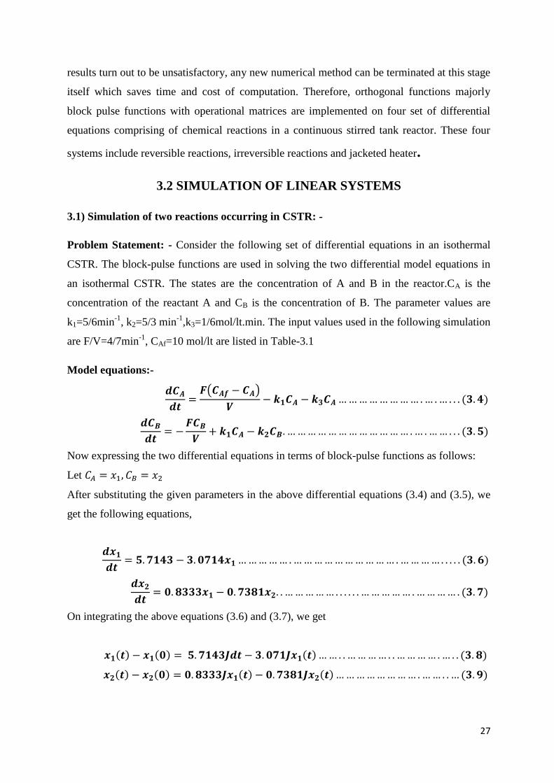
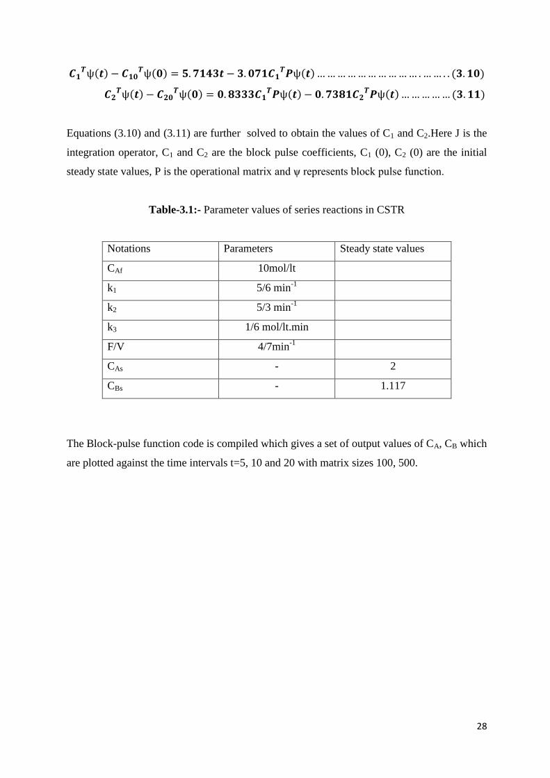
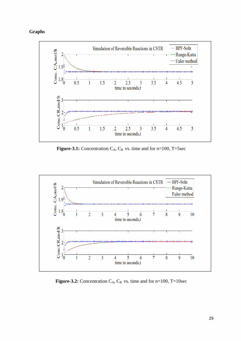
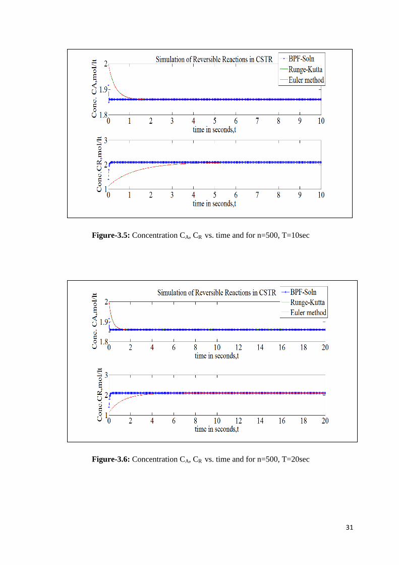
The Block-pulse function code is compiled which gives a set of output values of CA, CB which
are plotted against the time intervals t=5, 10 and 20 with matrix sizes 100, 500.
29
Graphs
Figure-3.1: Concentration CA, CR vs. time and for n=100, T=5sec
Figure-3.2: Concentration CA, CR vs. time and for n=100, T=10sec

30
Figure-3.3: Concentration CA, CR vs. time and for n=100, T=20sec
Figure-3.4: Concentration CA, CR vs. time and for n=500, T=5sec
31
Figure-3.5: Concentration CA, CR vs. time and for n=500, T=10sec
Figure-3.6: Concentration CA, CR vs. time and for n=500, T=20sec
32
3.2) Simulation of a Reversible reaction in a CSTR
Problem Statement:-Consider a set of differential equations for a first order reversible
reaction in an isothermal CSTR. The block-pulse functions are used in solving the two
differential model equations in an isothermal CSTR. The states are the concentration of A and
R in the reactor. CA is the concentration of the reactant A and CR is the concentration of R.
The parameter values are k1=0.125 min-1
; k2=0.325 min-1
. The input values used in the
following simulation are F/V=1/8min-1
, CAf=1000 mol/lt are listed in Table-3.2
Model Equations:-
𝒅𝑪𝑨
𝒅𝒕=
𝑭(𝑪𝑨𝒇 − 𝑪𝑨)
𝑽− 𝒌𝟏𝑪𝑨 + 𝒌𝟐𝑪𝑹. . . . . . … … … . . . . . … . . . . … … … … … … . . … . . . . (𝟑. 𝟏𝟐)
𝒅𝑪𝑩
𝒅𝒕= −
𝑭𝑪𝑹
𝑽+ 𝒌𝟏𝑪𝑨 − 𝒌𝟐𝑪𝑹. … … … . . . … … … . . . . . … … … . . . . . … … … . . . . . … … . . . . . (𝟑. 𝟏𝟑)
Now expressing the two differential equations in terms of block-pulse functions as follows:
Let 𝐶𝐴 = 𝑥1, 𝐶𝑅 = 𝑥2
After substituting the given parameters in the above differential equations (3.12) and (3.13),
we get the following equations,
𝒅𝒙𝟏
𝒅𝒕= 𝟏𝟐𝟓 − 𝟎. 𝟐𝟓𝒙𝟏 + 𝟎. 𝟑𝟐𝟓𝒙𝟐 … … … … … … … … . . . . . … . . . . … … … . … . (𝟑. 𝟏𝟒)
𝒅𝒙𝟐
𝒅𝒕= −𝟎. 𝟒𝟓𝒙𝟏 + 𝟎. 𝟏𝟐𝟓𝒙𝟐. . . . . . . . . . . . . . … … … … . . . . . . . . … … . … . . . (𝟑. 𝟏𝟓)
On integrating the above equations (3.14) and (3.15), we get
𝒙𝟏(𝒕) − 𝒙𝟏(𝟎) = 𝟏𝟐𝟓𝑱𝒅𝒕 − 𝟎. 𝟐𝟓𝑱𝒙𝟏(𝒕) + 𝟎. 𝟑𝟐𝟓𝑱𝒙𝟐(𝒕) … . . … . . … … … … . . (𝟑. 𝟏𝟔)
𝒙𝟐(𝒕) − 𝒙𝟐(𝟎) = −𝟎. 𝟒𝟓𝑱𝒙𝟏(𝒕) + 𝟎. 𝟏𝟐𝟓𝑱𝒙𝟐(𝒕) … … … … … … . . … … . . … … … (𝟑. 𝟏𝟕)
𝑪𝟏𝑻ѱ(𝒕) − 𝑪𝟏𝟎
𝑻ѱ(𝟎) = 𝟏𝟐𝟓𝒕 − 𝟎. 𝟐𝟓𝑪𝟏𝑻𝑷ѱ(𝒕) + 𝟎. 𝟑𝟐𝟓𝑪𝟐
𝑻𝑷ѱ(𝒕) … … … … . . … . . (𝟑. 𝟏𝟖)
𝑪𝟐𝑻ѱ(𝒕) − 𝑪𝟐𝟎
𝑻ѱ(𝟎) = −𝟎. 𝟒𝟓𝑪𝟏𝑻𝑷ѱ(𝒕) + 𝟎. 𝟏𝟐𝟓𝑪𝟐
𝑻𝑷ѱ(𝒕) … … … … . . … . (𝟑. 𝟏𝟗)
33
Equations (3.18) and (3.19) are further solved to obtain the values of C1 and C2.Here J is the
integration operator, C1 and C2 are the block pulse coefficients, C1 (0), C2 (0) are the initial
steady state values, P is the operational matrix and ѱ represents block pulse function.
Table-3.2:- Parameter values of reversible reaction
Notations Parameters Steady state values
CAf 1000mol/lt
k1 0.125 min-1
k2 0.325 min-1
k3 -
F/V 1/8min-1
CAs - 782.61
CRs - 217.39
The Block-pulse function, Runge-Kutta (MATLAB solver) and Euler method codes are
compiled which gives a set of output values of CA, CR which are plotted against the time
intervals t=10, 20 and 40 with matrix sizes 100 and 500.
Graphs:-
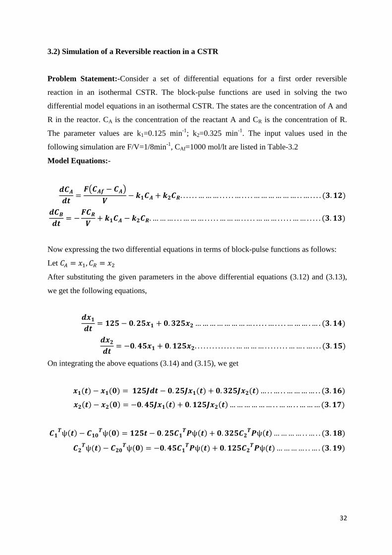
Figure-3.7: Concentration CA, CR vs. time and for n=100, T=10sec
34
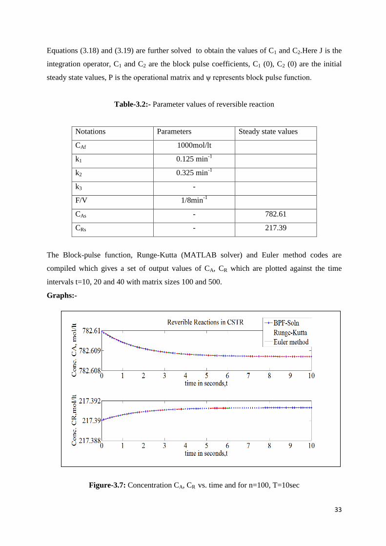
Figure-3.8: Concentration CA, CR vs. time and for n=500, T=10sec
Figure-3.9: Concentration CA, CR vs. time and for n=100, T=20sec
35
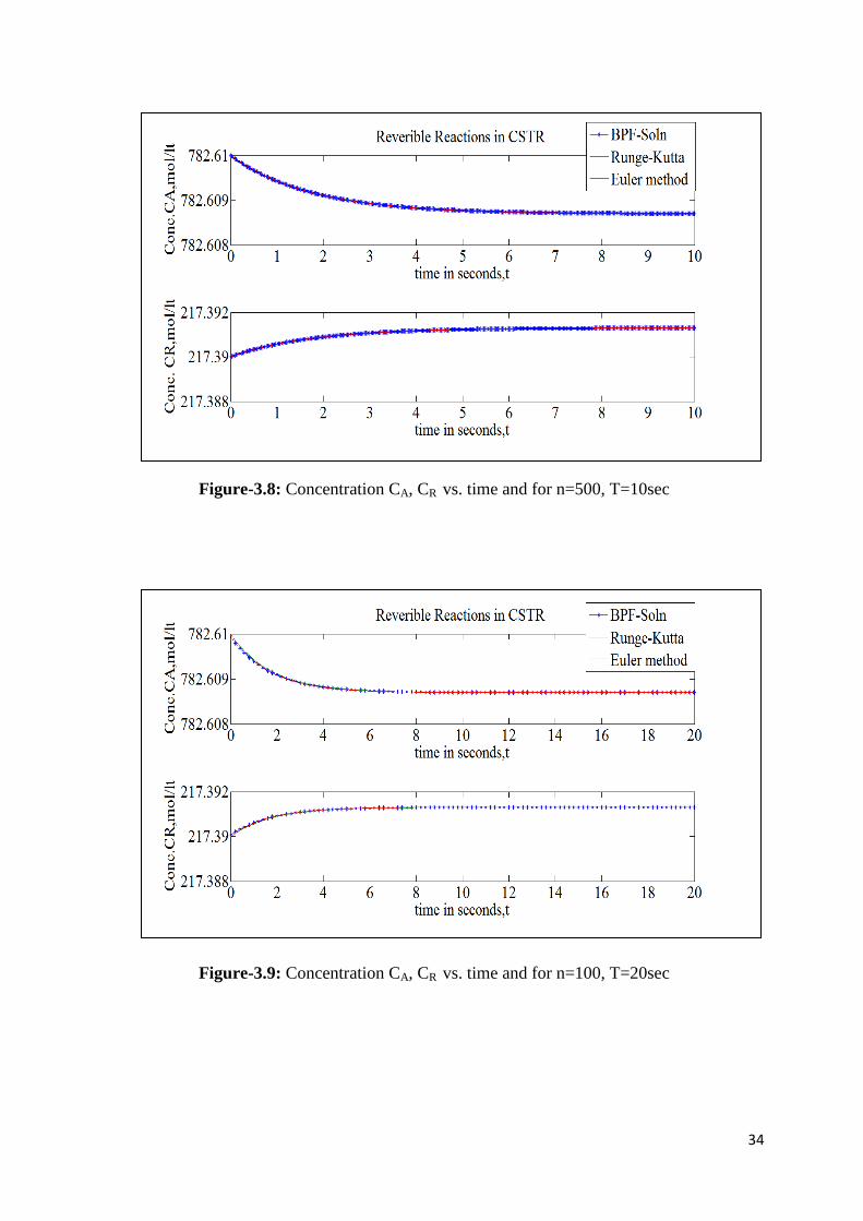
Figure-3.10: Concentration CA, CR vs. time and for n=500, T=20sec
Figure-3.10: Concentration CA, CR vs. time and for n=500, T=20sec
Figure-3.11: Concentration CA, CR vs. time and for n=100, T=40sec

36
Figure-3.12: Concentration CA, CR vs. time and for n=500, T=40sec
The above plots generated from BPF algorithm using MATLAB software and from Euler and
Runge-Kutta methods (inbuilt MATLAB solver ODE-45), represent the transient response to
initial conditions from steady state values, CAs=782.61, CRs=217.39.The new steady state
values reached by the CA and CR are 782.6088 and 217.3915 respectively. The plots show that
a similar trend in concentrations is observed with three kinds of data (BPF& Euler and Runge
–Kutta methods) obtained.
3.3) Simulation of an Irreversible Reaction in a CSTR
Problem Statement: - Consider a set of differential equations for a first order irreversible
reaction in an isothermal CSTR. Ethylene oxide (A) is reacted with water (B) to produce
ethylene glycol(R). Water is in large excess. A CSTR is used at a constant temperature. The
block-pulse functions are used in solving the two differential model equations in an isothermal
CSTR. The states are the concentration of A and R in the reactor. CA is the concentration of
the reactant A and CR is the concentration of R. The parameter values are k1=0.311 min-1
. The
input values used in the following simulation are F/V=0.0777min-1
, CAf =0.5mol/lt are listed
in Table-3.3
37
Model Equations:-
𝒅𝑪𝑨
𝒅𝒕=
𝑭(𝑪𝑨𝒇 − 𝑪𝑨)
𝑽− 𝒌𝟏𝑪𝑨. . . . . . . . . . . . . . . . . . . … … … … … … … … … … . … … . . . . . . . . . . . (𝟑. 𝟐𝟎)
𝒅𝑪𝑹
𝒅𝒕= −
𝑭𝑪𝑹
𝑽+ 𝒌𝟏𝑪𝑨. . . . . . . . . . . . . . . . . . . . . . . . . . . . … … … … … … … … … … … . . . . . . . . . . . . (𝟑. 𝟐𝟏)
Now expressing the two differential equations in terms of block-pulse functions as follows:
Let 𝐶𝐴 = 𝑥1, 𝐶𝑅 = 𝑥2
After substituting the given parameters in the above differential equations (3.22) and (3.23)
we get the following equations,
𝒅𝒙𝟏
𝒅𝒕= 𝟎. 𝟎𝟑𝟖𝟗 − 𝟎. 𝟑𝟖𝟖𝟕𝒙𝟏. . . . . . . . . . . . . . . . . . . . . … … … … … … … … … … … . . . . . (𝟑. 𝟐𝟐)
𝒅𝒙𝟐
𝒅𝒕= 𝟎. 𝟑𝟏𝟏𝒙𝟏 + 𝟎. 𝟎𝟕𝟕𝟕𝒙𝟐 … … … … … … … … … … … … … … … … … … … … . (𝟑. 𝟐𝟑)
On integrating the above equations (3.24) and (3.25), we get
𝒙𝟏(𝒕) − 𝒙𝟏(𝟎) = 𝟎. 𝟎𝟑𝟖𝟗𝑱𝒅𝒕 − 𝟎. 𝟑𝟖𝟖𝟕𝑱𝒙𝟏(𝒕). . . . . . . … … … . … … … … … . . . . . (𝟑. 𝟐𝟒)
𝒙𝟐(𝒕) − 𝒙𝟐(𝟎) = 𝟎. 𝟑𝟏𝟏𝑱𝒙𝟏(𝒕) + 𝟎. 𝟎𝟕𝟕𝟕𝑱𝒙𝟐(𝒕) … … … … … … … . … … … . . . . . (𝟑. 𝟐𝟓)
𝑪𝟏𝑻ѱ(𝒕) − 𝑪𝟏𝟎
𝑻ѱ(𝟎) = 𝟎. 𝟎𝟑𝟖𝟗𝒕 − 𝟎. 𝟑𝟖𝟖𝟕𝑪𝟏𝑻𝑷ѱ(𝒕) … … … … … … … … … … … … . . (𝟑. 𝟐𝟔)
𝑪𝟐𝑻ѱ(𝒕) − 𝑪𝟐𝟎
𝑻𝑷ѱ(𝟎) = 𝟎. 𝟑𝟏𝟏𝑪𝟏𝑻𝑷ѱ(𝒕) + 𝟎. 𝟎𝟕𝟕𝟕𝑪𝟐
𝑻𝑷ѱ(𝒕) … … … … … … . . … . . (𝟑. 𝟐𝟕)
Equations (3.26) and (3.27) are further solved to obtain the values of C1 and C2.Here J is the
integration operator, C1 and C2 are the block pulse coefficients, C1 (0), C2 (0) are the initial
steady state values, P is the operational matrix and ѱ represents block pulse function.
38
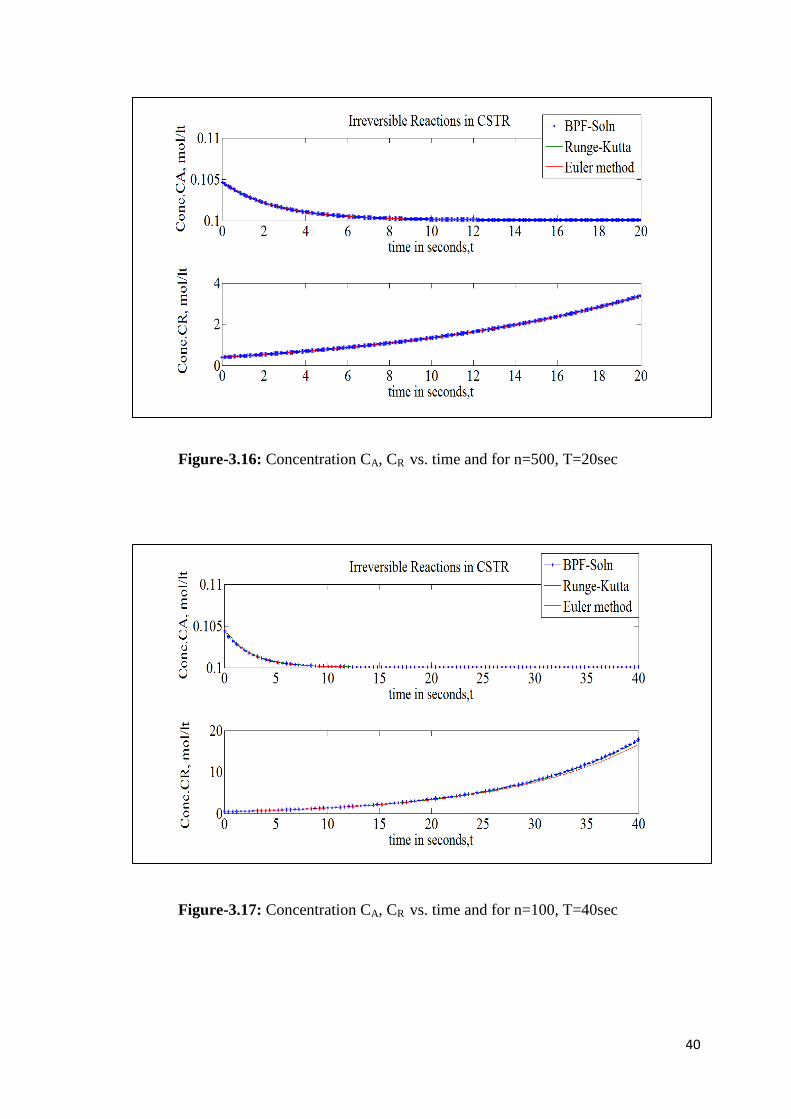
Table-3.3:- Parameter values of irreversible reactions in CSTR
Notations Parameters Steady state values
CAf 0.5mol/lt
k1 0.311 min-1
k2 -
k3 -
F/V 0.0777min-1
CAs - 0.1047
CRs - 0.395
The Block-pulse function, Runge-Kutta (MATLAB solver) and Euler method codes are
compiled which gives a set of output values of CA, CR which are plotted against the time
intervals t=10, 20 and 40 with matrix sizes 100 and 500.
Graphs
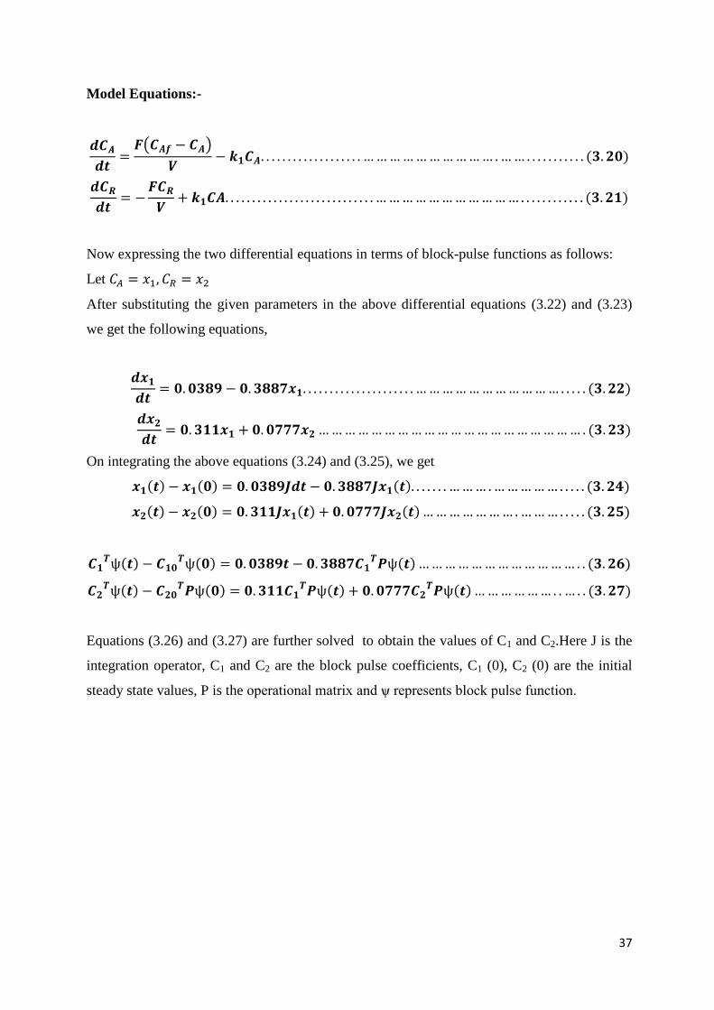
Figure-3.13: Concentration CA, CR vs. time and for n=100, T=10sec
39
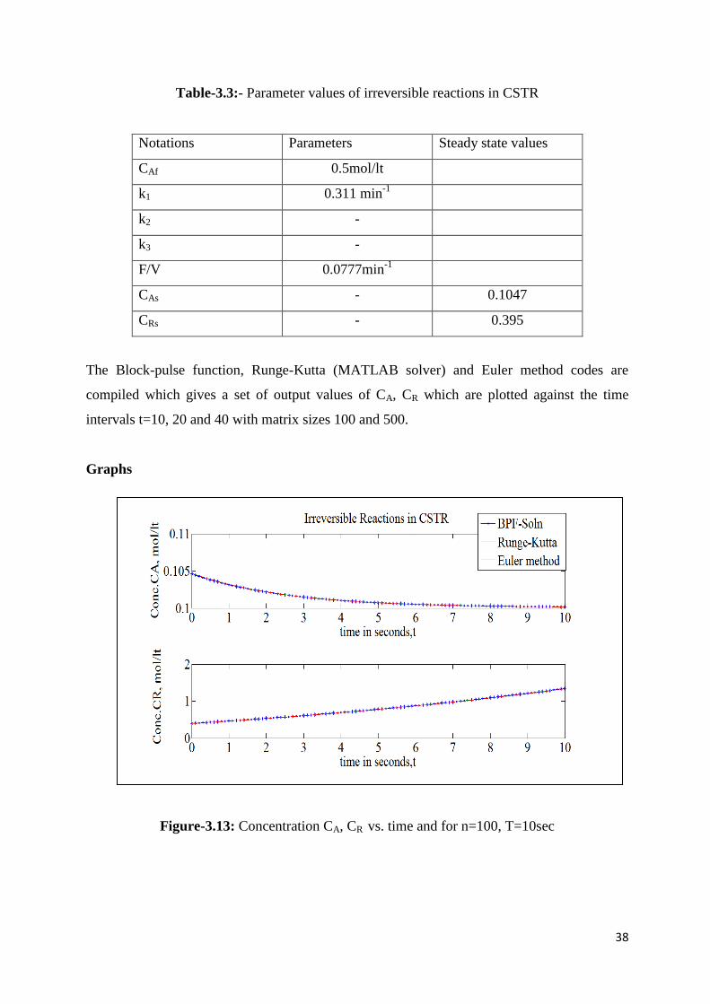
Figure-3.14: Concentration CA, CR vs. time and for n=500, T=10sec
Figure-3.15: Concentration CA, CR vs. time and for n=100, T=20sec
40
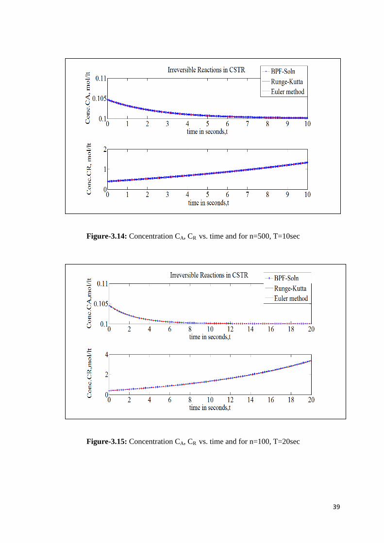
Figure-3.16: Concentration CA, CR vs. time and for n=500, T=20sec
Figure-3.17: Concentration CA, CR vs. time and for n=100, T=40sec
41
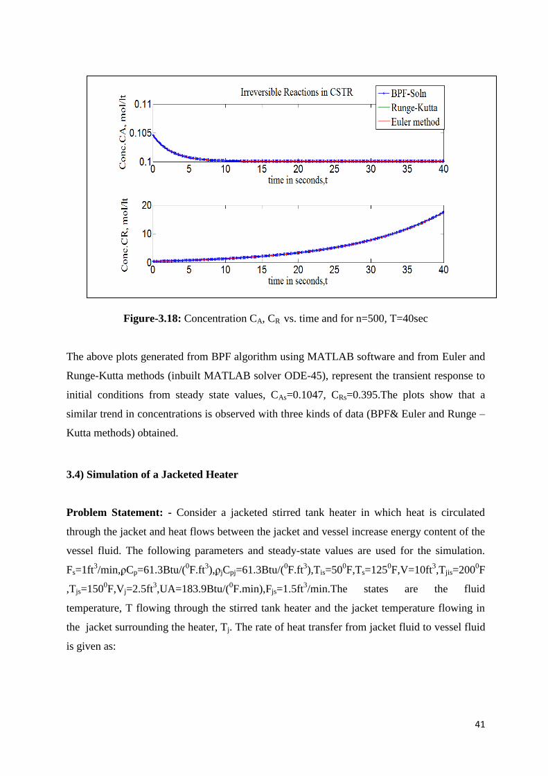
Figure-3.18: Concentration CA, CR vs. time and for n=500, T=40sec
The above plots generated from BPF algorithm using MATLAB software and from Euler and
Runge-Kutta methods (inbuilt MATLAB solver ODE-45), represent the transient response to
initial conditions from steady state values, CAs=0.1047, CRs=0.395.The plots show that a
similar trend in concentrations is observed with three kinds of data (BPF& Euler and Runge –
Kutta methods) obtained.
3.4) Simulation of a Jacketed Heater
Problem Statement: - Consider a jacketed stirred tank heater in which heat is circulated
through the jacket and heat flows between the jacket and vessel increase energy content of the
vessel fluid. The following parameters and steady-state values are used for the simulation.
Fs=1ft3/min,ϼCp=61.3Btu/(
0F.ft
3),ϼjCpj=61.3Btu/(
0F.ft
3),Tis=50
0F,Ts=125
0F,V=10ft
3,Tjis=200
0F
,Tjs=1500F,Vj=2.5ft
3,UA=183.9Btu/(
0F.min),Fjs=1.5ft
3/min.The states are the fluid
temperature, T flowing through the stirred tank heater and the jacket temperature flowing in
the jacket surrounding the heater, Tj. The rate of heat transfer from jacket fluid to vessel fluid
is given as:

42
Model Equations:-
𝑸 = 𝑼𝑨(𝑻𝒋 − 𝑻) … … … … … … … … … … … … … … … … … … … … … … … … … … … . … … (𝟑. 𝟐𝟖)
𝒅𝑻
𝒅𝒕 =
𝑭(𝑻𝒊 − 𝑻)
𝑽 +
𝑼𝑨(𝑻𝒋 − 𝑻)
𝑽𝝆𝑪𝒑. … … … … … … … … … … … … … … … … … … … . . . . . … (𝟑. 𝟐𝟗)
𝒅𝑻𝒋
𝒅𝒕= −
𝑭𝒋(𝑻𝒋𝒊𝒏 − 𝑻𝒋)
𝑽𝒋−
𝑼𝑨(𝑻𝒋 − 𝑻)
𝑽𝒋𝝆𝒋𝑪𝒑𝒋… … … … … … … … … … … … … … … … … … … . . (𝟑. 𝟑𝟎)
Now expressing the two differential equations in terms of block-pulse functions as follows:
Let 𝑇 = 𝑥1, 𝑇𝑗 = 𝑥2
After substituting the given parameters in the above differential equations, we get the
following equations,
𝒅𝒙𝟏
𝒅𝒕= 𝟓𝟏. 𝟐𝟒𝟓 − 𝟎. 𝟒𝟎𝟖𝟑𝒙𝟏 + 𝟎. 𝟑𝒙𝟐. . . . . . . . . . . . . . . . . . … … … … … . … . . . . . . . (𝟑. 𝟑𝟏)
𝒅𝒙𝟐
𝒅𝒕= 𝟏𝟐𝟎 + 𝟏. 𝟐𝒙𝟏 − 𝟏. 𝟖𝒙𝟐. . . . . . . . . … … … … … … … . . . . . . . . . . (𝟑. 𝟑𝟐)
On integrating the above equations (3.31) and (3.32) we get
𝒙𝟏(𝒕) − 𝒙𝟏(𝟎) = 𝟓𝟏. 𝟐𝟒𝟓𝑱𝒅𝒕 − 𝟎. 𝟒𝟎𝟖𝟑𝑱𝒙𝟏(𝒕) + 𝟎. 𝟑𝑱𝒙𝟐(𝒕) … … … … … . … . . (𝟑. 𝟑𝟑)
𝒙𝟐(𝒕) − 𝒙𝟐(𝟎) = 𝟏𝟐𝟎𝒕 + 𝟏. 𝟐𝑱𝒙𝟏(𝒕) − 𝟏. 𝟖𝑱𝒙𝟐(𝒕) … … … … … . . … … … … . . . . . . (𝟑. 𝟑𝟒)
𝑪𝟏𝑻ѱ(𝒕) − 𝑪𝟏𝟎
𝑻ѱ(𝟎) = 𝟓𝟏. 𝟐𝟒𝟓𝒕 − 𝟎. 𝟒𝟎𝟖𝟑𝑪𝟏𝑻𝑷ѱ(𝒕) + 𝟎. 𝟑𝑪𝟐
𝑻𝑷ѱ(𝒕) … … … … … . (𝟑. 𝟑𝟓)
𝑪𝟐𝑻ѱ(𝒕) − 𝑪𝟐𝟎
𝑻ѱ(𝟎) = 𝟏𝟐𝟎𝒕 + 𝟏. 𝟐𝑪𝟏𝑻𝑷ѱ(𝒕) − 𝟏. 𝟖𝑪𝟐
𝑻𝑷ѱ(𝒕) … … … … …. (𝟑. 𝟑𝟔)
Equations (3.35) and (3.36) are further solved to obtain the values of C1 and C2.Here J is the
integration operator, C1 and C2 are the block pulse coefficients, C1 (0), C2 (0) are the initial
steady state values, P is the operational matrix and ѱ represents block pulse function.
43
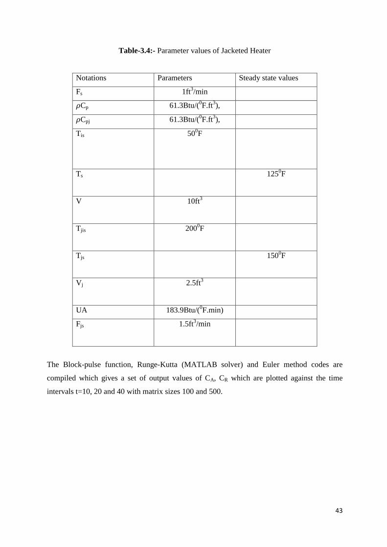
Table-3.4:- Parameter values of Jacketed Heater
Notations Parameters Steady state values
Fs 1ft3/min
𝜌Cp 61.3Btu/(0F.ft
3),
𝜌Cpj 61.3Btu/(0F.ft
3),
Tis 500F
Ts 1250F
V 10ft3
Tjis 2000F
Tjs 1500F
Vj 2.5ft3
UA 183.9Btu/(0F.min)
Fjs 1.5ft3/min
The Block-pulse function, Runge-Kutta (MATLAB solver) and Euler method codes are
compiled which gives a set of output values of CA, CR which are plotted against the time
intervals t=10, 20 and 40 with matrix sizes 100 and 500.
44
Graphs
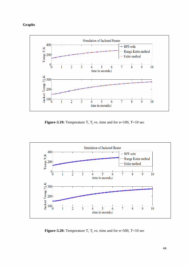
Figure-3.19: Temperature T, Tj vs. time and for n=100, T=10 sec
Figure-3.20: Temperature T, Tj vs. time and for n=500, T=10 sec
45
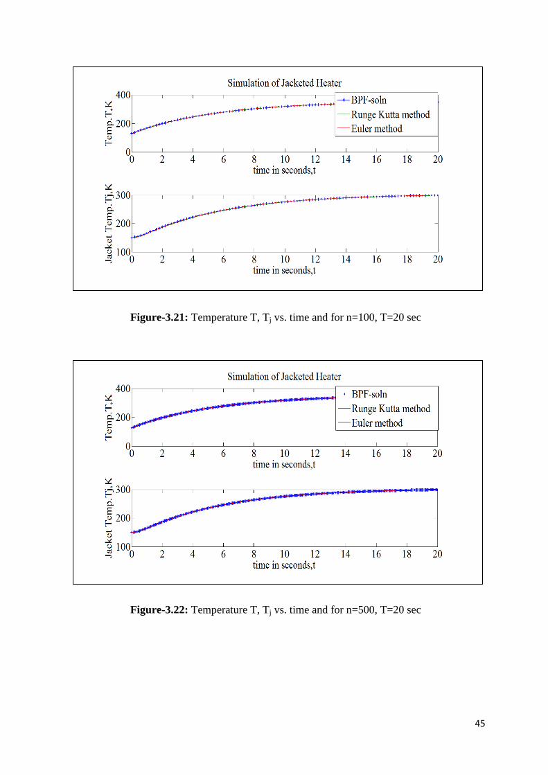
Figure-3.21: Temperature T, Tj vs. time and for n=100, T=20 sec
Figure-3.22: Temperature T, Tj vs. time and for n=500, T=20 sec
46
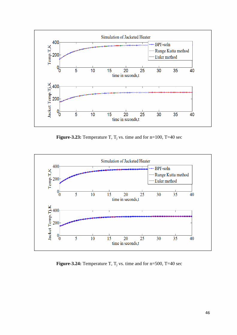
Figure-3.23: Temperature T, Tj vs. time and for n=100, T=40 sec
Figure-3.24: Temperature T, Tj vs. time and for n=500, T=40 sec
47
The above plots generated from BPF algorithm using MATLAB software and from Euler and
Runge-Kutta methods (inbuilt MATLAB solver ODE-45), represent the transient response to
initial conditions from steady state values, Ts=125,Tjs=150. The plots show that a similar
trend in temperatures is observed with three the kinds of data (BPF& Euler and Runge –Kutta
methods) obtained.
3.2.1 Results and Discussions
The state/output obtained from dynamic simulation using block-pulse functions (BPF)
is plotted against time. This plot is compared with the plots generated using Euler
method and Runge-Kutta method (MATLAB solver ODE-45). The plots are in a good
agreement to each other, which proves the potency of BPF for simulation of such
kinds of systems considered.
Consistent results are obtained for matrix dimensions 100 and 500 at various time
intervals such as 10, 20 and 40 seconds. Similarly, results can be extended further to
other matrix dimensions.
For small time intervals, the plots show a drop or an increase in concentration in a
linear manner. However as time proceeds, i.e. for large time intervals, the complete
curve gets developed. Thus, the results of all four simulations are in a good fit with
each other.
With small operational matrix size, there may be a deviation in the results of BPF
compared to those obtained using other numerical methods such as Euler and Runge-
Kutta. However, as the operational matrix size increases largely, the deviation from
the two solutions reduces. Besides existing numerical techniques, block pulse
functions also provide an efficient solution for the CSTR simulation.
48
3.3 NON LINEAR SYSTEMS
According to physics and other sciences, a nonlinear system does not obey the superposition
principle – which means the output of the system is not directly related to the input, contrary
to the linear systems. Many physical quantities have an upper bound which once reached the
system loses linearity; these quantities are vehicle’s velocity or electrical signals. The
differential equations of some thermal, biological systems are inherently nonlinear in nature.
Thus considering the non-linearity directly while analysing and designing controllers for such
systems is always an advantage. In addition, many mechanical systems are subject to non-
linearity by friction. Relays, which are part of many practical control systems, are inherently
nonlinear. Other examples include ferromagnetic cores in electrical machines and
transformers are often described with nonlinear magnetization curves and equations.
Mathematically, a nonlinear system of equations is defined as the set of simultaneous
equations in which the unknowns (or the unknown functions in the case of differential
equations) appear as variables of a polynomial of degree higher than one. Otherwise, it can be
defined as that system of equations to be solved which cannot be written as a linear
combination of unknown variables or functions that appear in it (them). Non-linearity in
known functions within the equations is treated insignificant. A differential equation is linear
if it is linear in terms of the unknown function and its derivatives, even if nonlinear in terms of
the other variables appearing in it. A nonlinear system of equations describes the behaviour of
a nonlinear system.
Engineers, physicists, mathematicians and many other scientists are primarily interested in
nonlinear problems because of their inherent nonlinear in nature. Because of the difficulty
involved in solving nonlinear equations, they are commonly approximated by linear equations
(linearization). Linearization achieves some amount of accuracy and some range for the input
values, but some interesting phenomena such as chaos and singularities are hidden. Behaviour
of a nonlinear system can be characterized to be chaotic, unpredictable or counter intuitive.
Although such chaotic behaviour may resemble random behaviour, it is absolutely not
random. For example, some aspects of the weather are seen to be chaotic, where the system
becomes very sensitive for small changes in inputs producing complex effects throughout.
Thus accurate long-term forecasts are impossible with current technology because of non-
linearity in systems.

49
3.3.1 Differences between Linear and Nonlinear systems:-
Linear systems obey the properties of superposition and homogeneity.
Non-Linear systems do not obey superposition and homogeneity.
Linear systems possess one equilibrium point at the origin while many equilibrium
points are possessed by non-linear systems.
For nonlinear systems, stability needs to be defined precisely.
For forced response for the nonlinear systems principle of superposition does not hold
good.
Linearity cannot be classified however Non-linearity can be broadly classified.
3.3.2 Definition of Linear and Nonlinear Systems:-
Linear systems must obey two important properties, superposition and homogeneity.
According to the principle of superposition for two different inputs, x and y, in the domain of
the function f,
𝒇(𝒙 + 𝒚) = 𝒇(𝒙) + 𝒇(𝒚) … … … … … … … … … … … … … … … … … … … … … … … … . … … (𝟑. 𝟑𝟕)
The property of homogeneity states that for a given input, x, in the domain of the function f,
and for any real number k,
𝒇(𝒌𝒙) = 𝒌𝒇(𝒙) … … … … … … … … … … … … … … … … … … … … … … … … . . … … … . . … … (𝟑. 𝟑𝟖)
Any function that does not satisfy superposition and homogeneity is non-linear; there is no
unifying characteristic of nonlinear systems, except for not satisfying the two above-
mentioned properties.
Linear Time Invariant (LTI) systems are commonly described by the equation:
𝒅𝒙
𝒅𝒕= 𝑨𝒙 + 𝑩𝒖 … … … … … … … … … … … … … … … … … … … … … … … … . … … … … … … . (𝟑. 𝟑𝟗)
In this equation, x is the vector of n state variables, u is the control input, and A is a matrix of
size (n-by-n), and B is a vector of appropriate dimensions. The equation determines the
dynamics of the response. It is sometimes called a state-space realization of the system.
Non-Linear Systems are commonly described by the equation:
𝒅𝒙
𝒅𝒕= 𝒇(𝒙) … … … … … … … … … … … … … … … … … … … … … … … … … … … … . … … . … . . (𝟑. 𝟒𝟎)
50
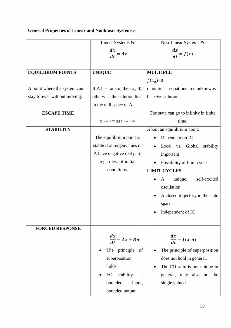
General Properties of Linear and Nonlinear Systems:-
Linear Systems &
𝒅𝒙
𝒅𝒕= 𝑨𝒙
Non-Linear Systems &
𝒅𝒙
𝒅𝒕= 𝒇(𝒙)
EQUILIBIUM POINTS
A point where the system can
stay forever without moving.
UNIQUE
If A has rank n, then 𝑥𝑒=0,
otherwise the solution lies
in the null space of A.
MULTIPLE
𝑓(𝑥𝑒)=0
n nonlinear equations in n unknowns
0 → +∞ solutions
ESCAPE TIME
x → +∞ as t → +∞
The state can go to infinity in finite
time.
STABILITY
The equilibrium point is
stable if all eigenvalues of
A have negative real part,
regardless of initial
conditions.
About an equilibrium point:
Dependent on IC
Local vs. Global stability
important
Possibility of limit cycles
LIMIT CYCLES
A unique, self-excited
oscillation
A closed trajectory in the state
space
Independent of IC
FORCED RESPONSE
𝒅𝒙
𝒅𝒕= 𝑨𝒙 + 𝑩𝒖
The principle of
superposition
holds.
I/O stability →
bounded input,
bounded output
𝒅𝒙
𝒅𝒕= 𝒇(𝒙, 𝒖)
The principle of superposition
does not hold in general.
The I/O ratio is not unique in
general, may also not be
single valued.
51
Sinusoidal input →
sinusoidal output
of same frequency
CHAOS
Complicated steady-state behavior,
may exhibit randomness despite the
deterministic nature of the system.
3.3.3 Non Linear Differential Equations:-
A system of differential equations not obeying homogeneity and superposition are said to be
nonlinear. Extremely diverse are problems involving nonlinear differential equations, and
methods of solution or analysis are problem dependent and cannot be generalized. The
Navier–Stokes equations in fluid dynamics, Lotka–Volterra equations in biology and Non-
Isothermal CSTR in reaction engineering are some of the important examples of nonlinear
differential equations.
A combination of known solutions into new solutions is not generally possible when dealing
with nonlinear problems which can be regarded as one of the greatest difficulties. A family of
linearly independent solutions can be used to construct general solutions through the
superposition principle for linear systems. A good example of this is one-dimensional heat
transport with Dirichlet boundary conditions, the solution of which can be written as a time-
dependent linear combination of sinusoids of differing frequencies; making solutions very
flexible. For nonlinear equations, several very specific solutions can be found very often;
however new solutions cannot be constructed as it does not satisfy the superposition principle.
Ordinary differential equations:-
First order ordinary differential equations are often exactly solved by separation of variables,
especially for autonomous equations. For example, the nonlinear equation
𝒅𝒖
𝒅𝒙= −𝒖𝟐 … … … … … … … … … … … … … … … … … … … … … … … … … … … … … … … … . . (𝟑. 𝟒𝟏)
𝒖 =𝟏
𝒙 + 𝒄… … … … … … … … … … … … … … … … … … … … … … … … … … … . … … … … … . (𝟑. 𝟒𝟐)
has eq-5 as a general solution (and also u = 0 as a particular solution, corresponding to the
limit of the general solution when C tends to the infinity). The equation is nonlinear because it
may be written as
52
𝒅𝒖
𝒅𝒙+ 𝒖𝟐 … … . … … … … … … … … … … … … … … … … . … … … … … … … … … … …. (𝟑. 𝟒𝟑)
and the left-hand side of the equation is not a linear function of u and its derivatives. Note that
if the u2 term were replaced with u, the problem would be linear (the exponential
decay problem).
Second and higher order ordinary differential equations (more generally, systems of nonlinear
equations) rarely yield closed form solutions, though implicit solutions and solutions
involving non-elementary integrals are encountered.
Common methods for the qualitative analysis of nonlinear ordinary differential equations
include:
Examination of any conserved quantities, especially in Hamiltonian systems.
Examination of dissipative quantities (see Lyapunov function) analogous to conserved
quantities.
Linearization via Taylor expansion.
Change of variables into something easier to study.
Bifurcation theory.
Perturbation methods
3.4 SIMULATION OF NON-LINEAR SYSTEMS
Blood Glucose Control in Diabetic Patients:-
There are many innate feedback control loops within a human body. For instance, pancreas
regulates blood glucose by producing insulin. Food is consumed and later broken down by the
digestive system; as a result blood glucose level rises which in turn stimulates insulin
production. Glucose is broken down by the cells with the help of insulin. Insulin is not
produced by diabetes mellitus patients of Type I .Hence patient must be administered insulin
shots at several regular time intervals to regulate the blood glucose level. Thus, a typical
patient here is serving as a control system. Administration of insulin shots coinciding with the
meal concentration comprises the feed forward control nature. Other actions such as dosage
changes based on glucose measurements obtained from finger pricks and analysis of glucose
53
strips. Hyperglycaemia leads to blindness, cardiovascular problems in the long run while
fainting, diabetic comas are problems due to it in the short run.
Development of closed-loop insulin delivery systems has been highly motivated and external
pumps provided with insulin reservoirs which can deliver insulin directly instead of shots are
used by the current technology.
3.5) Problem Statement: - Consider a diabetic that is modelled using the following set of
parameters
Model equations:-
𝒅𝑮
𝒅𝒕= −𝒑𝟏𝑮 − 𝒙(𝑮𝒃 + 𝑮) +
𝑮𝒎𝒆𝒂𝒍
𝑽𝟏… … … … … … … … … … … … … … … … … … … . . … … (𝟑. 𝟒𝟒)
𝒅𝑿
𝒅𝒕= −𝒑𝟐𝑿 + 𝒑𝟑𝑰 … … … … … … … … … … … … … … … … … … … … … … … … … … … … … (𝟑. 𝟒𝟓)
𝒅𝑰
𝒅𝒕= −𝒏(𝑰 + 𝑰𝒃) +
𝑼
𝑽𝟏… … … … … … … … … … … … … … … … … … … … … … … … … … . … (𝟑. 𝟒𝟔)
Where G and I represent the deviation in blood glucose and insulin concentrations
respectively. Also X is proportional to insulin concentration in a remote compartment. The
inputs are 𝑮𝒎𝒆𝒂𝒍, a meal disturbance input of glucose, U manipulated insulin infusion rate.
The parameters include 𝒑𝟏, 𝒑𝟐, 𝒑𝟑, 𝒏, 𝑽𝟏.Other parameters are 𝑮𝒃, 𝑰𝒃 are the basal values of
blood and insulin concentration. These values are used to determine the basal infusion rate of
insulin necessary to maintain a steady state.
Let G=𝑥1, X=𝑥2, I=𝑥3
After substituting the given parameters in the above differential equations, we get the
following equations:
𝒅𝒙𝟏
𝒅𝒕= −𝟏𝟔. 𝟔𝟔𝟕𝒙𝟏 − 𝟒. 𝟓𝒙𝟐 − 𝒙𝟏𝒙𝟐 + 𝟎. 𝟑𝟕𝟓 … … … … … … . … … … … … … … … … … . (𝟑. 𝟒𝟕)
𝒅𝒙𝟐
𝒅𝒕= −𝟎. 𝟎𝟐𝟓𝒙𝟐 + 𝟎. 𝟎𝟎𝟎𝟎𝟏𝟑𝒙𝟑 … … … … … … … … … … … … … … … … … … … . … … . (𝟑. 𝟒𝟖)
𝒅𝒙𝟑
𝒅𝒕= −𝟎. 𝟎𝟗𝟐𝟔𝒙𝟑 + 𝟎. 𝟗𝟕𝟐𝟐 … … … … … … … … … … … … … … … … . … … … … … … … . (𝟑. 𝟒𝟗)
54
On integrating the above equations we get
𝒙𝟏(𝒕) − 𝒙𝟏(𝟎) = 𝟎. 𝟑𝟕𝟓𝑱𝒅𝒕 − 𝟏𝟔. 𝟔𝟔𝟕𝑱𝒙𝟏(𝒕) − 𝟎. 𝟒𝟓𝑱𝒙𝟐(𝒕) − 𝑱𝒙𝟏(𝒕)𝒙𝟐(𝒕). . (𝟑. 𝟓𝟎)
𝒙𝟐(𝒕) − 𝒙𝟐(𝟎) = −𝟎. 𝟎𝟐𝟓𝑱𝒙𝟐(𝒕) + 𝟎. 𝟎𝟎𝟎𝟎𝟏𝟑𝑱𝒙𝟑(𝒕) … … … … … … … . . . . . . . . (𝟑. 𝟓𝟏)
𝒙𝟑(𝒕) − 𝒙𝟑(𝟎) = −𝟎. 𝟎𝟗𝟐𝟔𝑱𝒙𝟑(𝒕) + 𝟎. 𝟗𝟕𝟐𝟐𝑱𝒅𝒕 … … … … … … … … … … … . … (𝟑. 𝟓𝟐)
𝑪𝟏𝑻ѱ(𝒕) − 𝑪𝟏𝟎
𝑻ѱ(𝟎) = 𝟎. 𝟑𝟕𝟓𝒕 − 𝟏𝟔. 𝟔𝟔𝟕𝑪𝟏𝑻𝑷ѱ(𝒕) − 𝟎. 𝟒𝟓𝑪𝟐
𝑻𝑷ѱ(𝒕) − 𝑪𝟏𝑻𝑷𝑪𝟐
𝑻𝑷ѱ(𝒕)
… … … … … … … … … … … … … … … … … … … . … . (𝟑. 𝟓𝟑)
𝑪𝟐𝑻ѱ(𝒕) − 𝑪𝟐𝟎
𝑻ѱ(𝟎) = −𝟎. 𝟎𝟐𝟓𝑪𝟐𝑻𝑷ѱ(𝒕) + 𝟎. 𝟎𝟎𝟎𝟎𝟏𝟑𝑪𝟑
𝑻𝑷ѱ(𝒕) … … …. (𝟑. 𝟓𝟒)
𝑪𝟑𝑻ѱ(𝒕) − 𝑪𝟑𝟎
𝑻ѱ(𝟎) = −𝟎. 𝟎𝟗𝟐𝟔𝑪𝟑𝑻𝑷ѱ(𝒕) + 𝟎. 𝟗𝟕𝟐𝟐𝒕 … … … … … … … . … . (𝟑. 𝟓𝟓)
Equations (3.53), (3.54) and (3.55) are further solved to obtain the values of C1,C2and
C3.Here J is the integration operator, C1,C2and C3are the block pulse coefficients, C1(0), C2 (0)
and C3(0)are the initial steady state values, P is the operational matrix and ѱ represents block
pulse function.
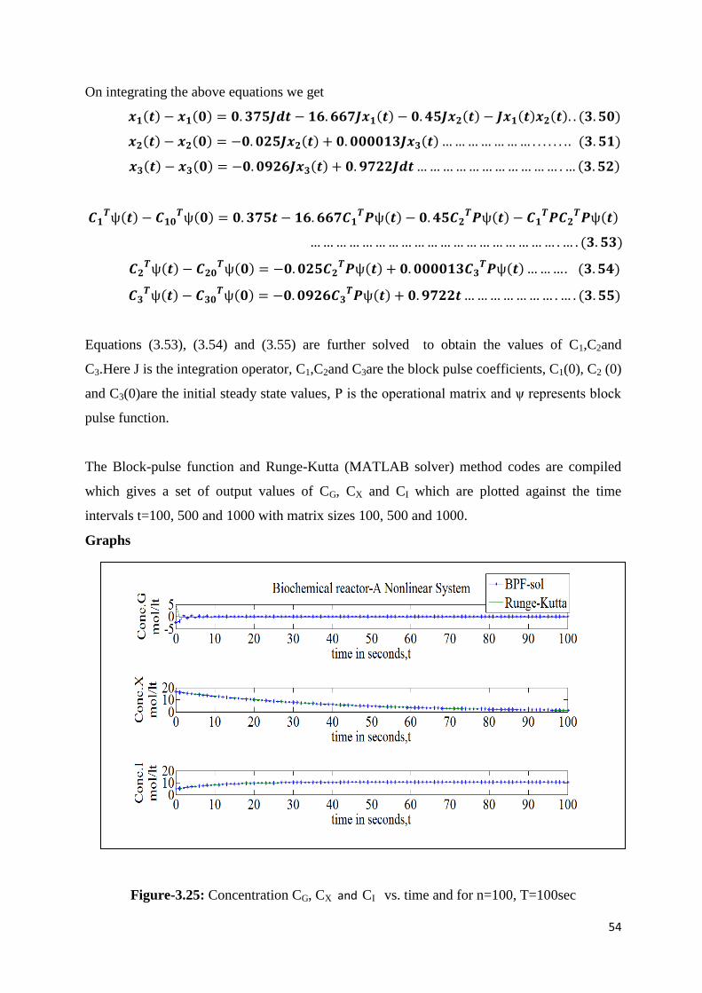
The Block-pulse function and Runge-Kutta (MATLAB solver) method codes are compiled
which gives a set of output values of CG, CX and CI which are plotted against the time
intervals t=100, 500 and 1000 with matrix sizes 100, 500 and 1000.
Graphs
Figure-3.25: Concentration CG, CX and CI vs. time and for n=100, T=100sec
55
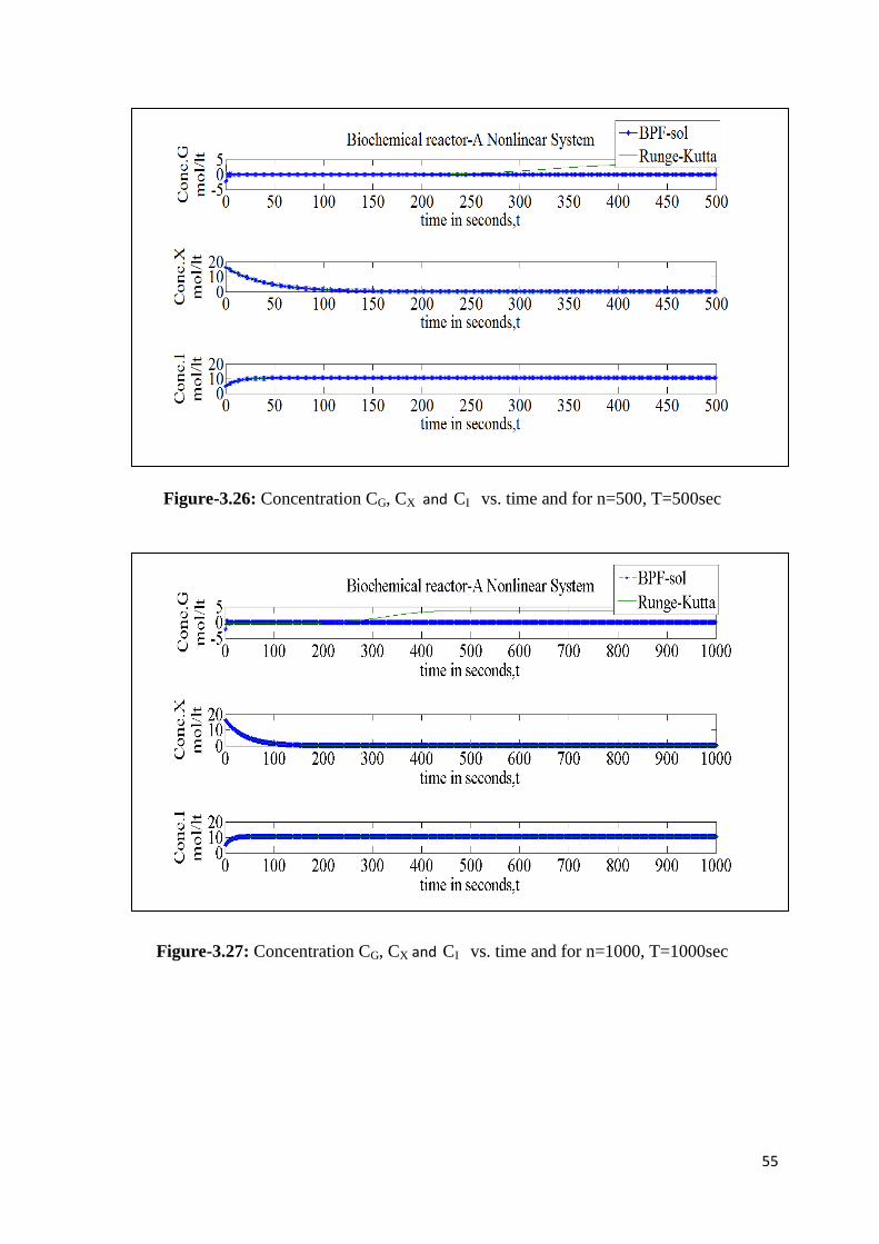
Figure-3.26: Concentration CG, CX and CI vs. time and for n=500, T=500sec
Figure-3.27: Concentration CG, CX and CI vs. time and for n=1000, T=1000sec

56
3.4.1 Results and Discussions
The given steady state values are 4.5, 16.667, 4.5 for G, X, I concentrations
respectively and new steady state values established are 0.02, 1.356, 10.4984
respectively.
For a matrix size of n=100, t=100 sec, a large aberration observed in the blood glucose
concentration, G plotted using BPF data from that of the plots obtained by MATLAB
solver ODE-45 data.
Similarly, for the same matrix size but at different time intervals, deviation in insulin
concentration (I), proportional concentration (X) are observed for plots obtained using
BPF data from that of the plots obtained by MATLAB solver ODE-45 data.
Deviations are observed to be minimizing with an increase in operational matrix sizes,
such as that observed for n=500, t=500sec in plot-2, and there is even small deviation
observed in concentrations of G, X, I for n=1000, t=1000sec.
By increasing the number of subintervals within an interval the accuracy obviously
increases because block pulse functions are binary in nature.
Large time intervals will not increase the computation time to a great extent as the
resulting operational matrix comprises of non-zero elements in the principal diagonal
of the matrix, zeroes in the upper triangular matrix and ones in lower triangular matrix
which makes computation simple even for large matrix sizes such as n=1000
57
CHAPTER-4
SIMULATION OF LINEAR AND NON-LINEAR
SYSTEMS VIA ORTHOGONAL FUNCTIONS
USING RECURRENCE RELATION
58
A Time- series is a sequence of data points measured typically at successive points in uniform
intervals of time. Two methods are available for time-series analysis: frequency domain
analysis, time domain analysis. Modern control theory essentially uses time domain approach
while conventional control theory uses frequency domain analysis. The present work is
premised on time domain approach in analysing the dynamic systems in chemical processes
using two important orthogonal functions: block pulse functions, linear triangular functions
via state space approach. By using vector-matrix notation, nth order differential equation may
be expressed as a first order vector-matrix differential equation. The state space approach uses
this vector-matrix notation to relate the input –output relationship. The knowledge of the state
variables of a dynamic system at initial value t=t0 combined with input at t≥t0 completely
determines the behaviour of the system for any time t≥t0 .
4.1 RECURRENCE RELATION USING TRIANGULAR FUNCTIONS
FOR LINEAR SYSTEMS
Consider the time –invariant linear SISO dynamic system modelled by
�̇� = 𝑨𝒙 + 𝑩𝒖 𝒂𝒏𝒅 𝒙(𝟎) = 𝒙𝟎 … … … … … … … … … … … … … … … … … … … … … … … … . . (𝟒. 𝟏)
∫ 𝒙(𝝉)̇
𝒕
𝟎
𝒅𝝉 = 𝒙(𝒕) − 𝒙(𝟎) … … … … … … … … … … … … … … … … … … … … … … … . … … . (𝟒. 𝟐)
Where, x is a state vector, u is an input vector, and A and B are matrices of appropriate
dimensions. The rate vector 𝑑𝑥
𝑑𝑡 , the state vector x and overall control vector Bu are expanded
into triangular function domain as given below:
𝒙(𝒕)̇ = ∑ 𝑪𝟏,𝒊+𝟏𝑻 𝑻𝟏,𝒊+𝟏(𝒕)
𝒎−𝟏
𝒊=𝟎
+ ∑ 𝑪𝟐,𝒊+𝟏𝑻 𝑻𝟐,𝒊+𝟏(𝒕)
𝒎−𝟏
𝒊=𝟎
≜ 𝑪𝟏𝑻𝟏(𝒕) + 𝑪𝟐𝑻𝟐(𝒕) … … … … . … (𝟒. 𝟑)
𝒙(𝒕) = ∑ 𝑫𝟏,𝒊+𝟏𝑻 𝑻𝟏,𝒊+𝟏(𝒕)
𝒎−𝟏
𝒊=𝟎
+ ∑ 𝑫𝟐,𝒊+𝟏𝑻 𝑻𝟐,𝒊+𝟏(𝒕)
𝒎−𝟏
𝒊=𝟎
≜ 𝑫𝟏𝑻𝟏(𝒕) + 𝑫𝟐𝑻𝟐(𝒕) … … … . . … (𝟒. 𝟒)
𝑩𝒖(𝒕) = ∑ 𝑬𝟏,𝒊+𝟏𝑻 𝑻𝟏,𝒊+𝟏(𝒕)
𝒎−𝟏
𝒊=𝟎
+ ∑ 𝑬𝟐,𝒊+𝟏𝑻 𝑻𝟐,𝒊+𝟏(𝒕)
𝒎−𝟏
𝒊=𝟎
≜ 𝑬𝟏𝑻𝟏(𝒕) + 𝑬𝟐𝑻𝟐(𝒕) … … . . . . … . (𝟒. 𝟓)

59
Here 𝐶1,𝑖+1, 𝐶2,𝑖+1, 𝐷1,𝑖+1,𝑖+1, 𝐷2,𝑖+1, 𝐸1,𝑖+1 and 𝐸2,𝑖+1 are n-vectors and form the (i+1)th
column of the n-by-m matrices 𝐶1, 𝐶2, 𝐷1, 𝐷2, 𝐸1 and 𝐸2 respectively.For a given input
u(t), 𝐸1 and 𝐸2 are known using the function approximation. To solve the state vector x in the
TF domain equation 2 is used.
Using equation 4.3 in equation 4.22 and the TF property of integration, we get
[𝑪𝟏 + 𝑪𝟐] ∫ 𝑻𝟏 (𝒕) = 𝑫𝟏𝑻𝟏(𝒕) + 𝑫𝟐𝑻𝟐(𝒕) − 𝟐𝒙�̃� … … … … … … … … . . … … . … … … … … (𝟒. 𝟔)
Using the TF property of integration and equation 1 and dropping the argument (t), we can
write
[𝑪𝟏 + 𝑪𝟐][𝑷𝟏𝑻𝟏 + 𝑷𝟐𝑻𝟐] = 𝑫𝟏𝑻𝟏 + 𝑫𝟐𝑻𝟏 − 𝒙�̃�[𝑻𝟏 + 𝑻𝟏] … … . … … … … . . … … . . … … . (𝟒. 𝟕)
Equating like coefficients of the basis functions T1 and T2, we obtain
[𝑪𝟏 + 𝑪𝟐]𝑷𝟏 = 𝑫𝟏 − 𝒙�̃� … … … … … … … … … … … … … … … … … . … … … … … … . … … . . (𝟒. 𝟖)
[𝑪𝟏 + 𝑪𝟐]𝑷𝟐 = 𝑫𝟐 − 𝒙�̃� … … … … … … … … … … … … … … … … … … … … … . … … . . . . … … . (𝟒. 𝟗)
Adding equations (4.8) and (4.9), we get
[𝑪𝟏 + 𝑪𝟐][𝑷𝟏 + 𝑷𝟐] = [𝑫𝟏 + 𝑫𝟐] − 𝟐𝒙�̃� … … … … … … … … … … … … … … … … … . … . . (𝟒. 𝟏𝟎)
Putting 𝐶1 + 𝐶2 ≜ 𝐶, 𝐷1 + 𝐷2 ≜ 𝐷 and using the relation 𝑃1 + 𝑃2 ≜ 𝑃, we have
𝑪𝑷 = 𝑫 − 𝟐𝒙�̃� … … … … … … … … … … … … … … … … … … … … … … … … … … … … … … … (𝟒. 𝟏𝟏)
(𝑪𝑷)𝒊+𝟏 = 𝑫𝒊+𝟏 − 𝟐𝒙�̃� … … … … … … … … … … … … … … … … … … … … … … … … … … … . (𝟒. 𝟏𝟐)
To proceed with the TF domain solution, we use the property of the matrix P and can write
(𝑪𝑷)𝒊+𝟏 =𝑻
𝒎∑ 𝑪𝒋 +
𝑻
𝟐𝒎𝑪𝒊+𝟏
𝒊
𝒋=𝟏
, 𝒊 ≤ 𝒋 … … … … … … … … … … … … … … … … … … … … . . (𝟒. 𝟏𝟑)
Writing in a recurrence relation form
(𝑪𝑷)𝟏 = 𝟐𝑻
𝒎𝑪𝟏 … … … … … … … … … … … … … … … … … … … … … … … … … … . … … . … . (𝟒. 𝟏𝟒)
(𝑪𝑷)𝒊+𝟐 = (𝑪𝑷)𝒊+𝟏 +𝑻
𝒎(𝑪𝒊+𝟏 + 𝑪𝟏𝒊+𝟐) … … … … … … … … . . … (𝟒. 𝟏𝟓)
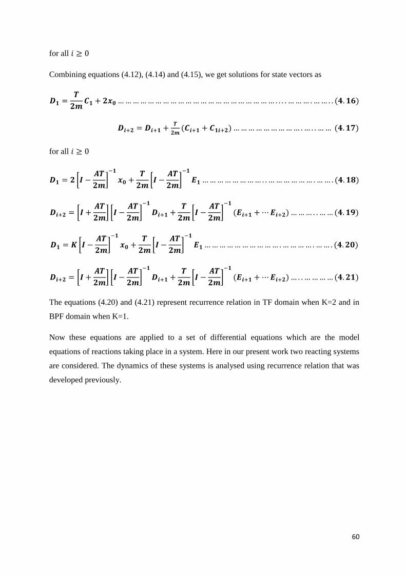
60
for all 𝑖 ≥ 0
Combining equations (4.12), (4.14) and (4.15), we get solutions for state vectors as
𝑫𝟏 =𝑻
𝟐𝒎𝑪𝟏 + 𝟐𝒙𝟎 … … … … … … … … … … … … … … … … … … … … … . . . . … … … . … … . . (𝟒. 𝟏𝟔)
𝑫𝒊+𝟐 = 𝑫𝒊+𝟏 +𝑻
𝟐𝒎(𝑪𝒊+𝟏 + 𝑪𝟏𝒊+𝟐) … … … … … … … … … . … . . … … (𝟒. 𝟏𝟕)
for all 𝑖 ≥ 0
𝑫𝟏 = 𝟐 [𝑰 −𝑨𝑻
𝟐𝒎]
−𝟏
𝒙𝟎 +𝑻
𝟐𝒎[𝑰 −
𝑨𝑻
𝟐𝒎]
−𝟏
𝑬𝟏 … … … … … … … … . . … … … … … … . … … . (𝟒. 𝟏𝟖)
𝑫𝒊+𝟐 = [𝑰 +𝑨𝑻
𝟐𝒎] [𝑰 −
𝑨𝑻
𝟐𝒎]
−𝟏
𝑫𝒊+𝟏 +𝑻
𝟐𝒎[𝑰 −
𝑨𝑻
𝟐𝒎]
−𝟏
(𝑬𝒊+𝟏 + ⋯ 𝑬𝒊+𝟐) … … … . . … … (𝟒. 𝟏𝟗)
𝑫𝟏 = 𝑲 [𝑰 −𝑨𝑻
𝟐𝒎]
−𝟏
𝒙𝟎 +𝑻
𝟐𝒎[𝑰 −
𝑨𝑻
𝟐𝒎]
−𝟏
𝑬𝟏 … … … … … … … … … … . … … … … . … … . (𝟒. 𝟐𝟎)
𝑫𝒊+𝟐 = [𝑰 +𝑨𝑻
𝟐𝒎] [𝑰 −
𝑨𝑻
𝟐𝒎]
−𝟏
𝑫𝒊+𝟏 +𝑻
𝟐𝒎[𝑰 −
𝑨𝑻
𝟐𝒎]
−𝟏
(𝑬𝒊+𝟏 + ⋯ 𝑬𝒊+𝟐) … . . … … … … (𝟒. 𝟐𝟏)
The equations (4.20) and (4.21) represent recurrence relation in TF domain when K=2 and in
BPF domain when K=1.
Now these equations are applied to a set of differential equations which are the model
equations of reactions taking place in a system. Here in our present work two reacting systems
are considered. The dynamics of these systems is analysed using recurrence relation that was
developed previously.
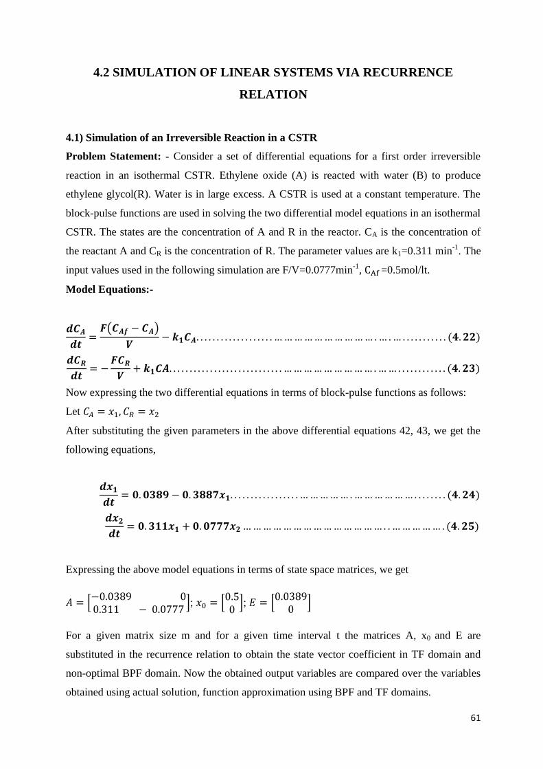
61
4.2 SIMULATION OF LINEAR SYSTEMS VIA RECURRENCE
RELATION
4.1) Simulation of an Irreversible Reaction in a CSTR
Problem Statement: - Consider a set of differential equations for a first order irreversible
reaction in an isothermal CSTR. Ethylene oxide (A) is reacted with water (B) to produce
ethylene glycol(R). Water is in large excess. A CSTR is used at a constant temperature. The
block-pulse functions are used in solving the two differential model equations in an isothermal
CSTR. The states are the concentration of A and R in the reactor. CA is the concentration of
the reactant A and CR is the concentration of R. The parameter values are k1=0.311 min-1
. The
input values used in the following simulation are F/V=0.0777min-1
, CAf =0.5mol/lt.
Model Equations:-
𝒅𝑪𝑨
𝒅𝒕=
𝑭(𝑪𝑨𝒇 − 𝑪𝑨)
𝑽− 𝒌𝟏𝑪𝑨. . . . . . . . . . . . . . . . . . . … … … … … … … … … … . … . … . . . . . . . . . . . (𝟒. 𝟐𝟐)
𝒅𝑪𝑹
𝒅𝒕= −
𝑭𝑪𝑹
𝑽+ 𝒌𝟏𝑪𝑨. . . . . . . . . . . . . . . . . . . . . . . . . . . . … … … … … … … … … . … … . . . . . . . . . . . . (𝟒. 𝟐𝟑)
Now expressing the two differential equations in terms of block-pulse functions as follows:
Let 𝐶𝐴 = 𝑥1, 𝐶𝑅 = 𝑥2
After substituting the given parameters in the above differential equations 42, 43, we get the
following equations,
𝒅𝒙𝟏
𝒅𝒕= 𝟎. 𝟎𝟑𝟖𝟗 − 𝟎. 𝟑𝟖𝟖𝟕𝒙𝟏. . . . . . . . . . . . . . . . . … … … … … . … … … … … … . . . . . . . . (𝟒. 𝟐𝟒)
𝒅𝒙𝟐
𝒅𝒕= 𝟎. 𝟑𝟏𝟏𝒙𝟏 + 𝟎. 𝟎𝟕𝟕𝟕𝒙𝟐 … … … … … … … … … … … … … … . . … … … … … . (𝟒. 𝟐𝟓)
Expressing the above model equations in terms of state space matrices, we get
𝐴 = [−0.0389 00.311 − 0.0777
]; 𝑥0 = [0.50
]; 𝐸 = [0.0389
0]
For a given matrix size m and for a given time interval t the matrices A, x0 and E are
substituted in the recurrence relation to obtain the state vector coefficient in TF domain and
non-optimal BPF domain. Now the obtained output variables are compared over the variables
obtained using actual solution, function approximation using BPF and TF domains.

62
The actual solution of the system is obtained as:
𝒙𝟏(𝒕) = −𝟎. 𝟎𝟗𝟔𝟓𝒆−𝟎.𝟎𝟕𝟕𝒕 + 𝟎. 𝟖𝟒𝟖𝟐𝒆−𝟎.𝟑𝟖𝟗𝒕 + 𝟎. 𝟏𝟎𝟎𝟔 … … … … … … … … … … . … … (𝟒. 𝟐𝟔)
𝒙𝟐(𝒕) = 𝟏. 𝟐𝟓𝟑𝒆−𝟎.𝟎𝟕𝟕𝒕 − 𝟐. 𝟏𝟖𝟎𝟓𝒆−𝟎.𝟑𝟖𝟗𝒕 + 𝟎. 𝟒𝟎𝟑𝟑 … … … … … … … … . … … … … … . (𝟒. 𝟐𝟕)
The function approximation using BPF and TF domain is given as following respectively:
𝒄𝒊,𝑩𝑷𝑭 =𝟏
𝒉∫ 𝒙𝟏(𝒕)𝜱𝒊(𝒕)𝒅𝒕
𝟏
𝟎
… … … … … … … … … … … … … … … … … … … … … … … … . . (𝟒. 𝟐𝟖)
𝒄𝒊,𝑻𝑭 = 𝒙𝟏(𝒊𝒉); 𝒅𝒊 = 𝒙𝟏((𝒊 + 𝟏)𝒉) … … … … … … … … … … … … … … … … … … … … … . . (𝟒. 𝟐𝟗)
The results are plotted using MATLAB against various time intervals, t=10,50 and 100 sec for
various matrix sizes, m=10,50 and 100 as shown below:
Figure-4.1: Concentration CA, CP vs. time and for n=10, T=10sec
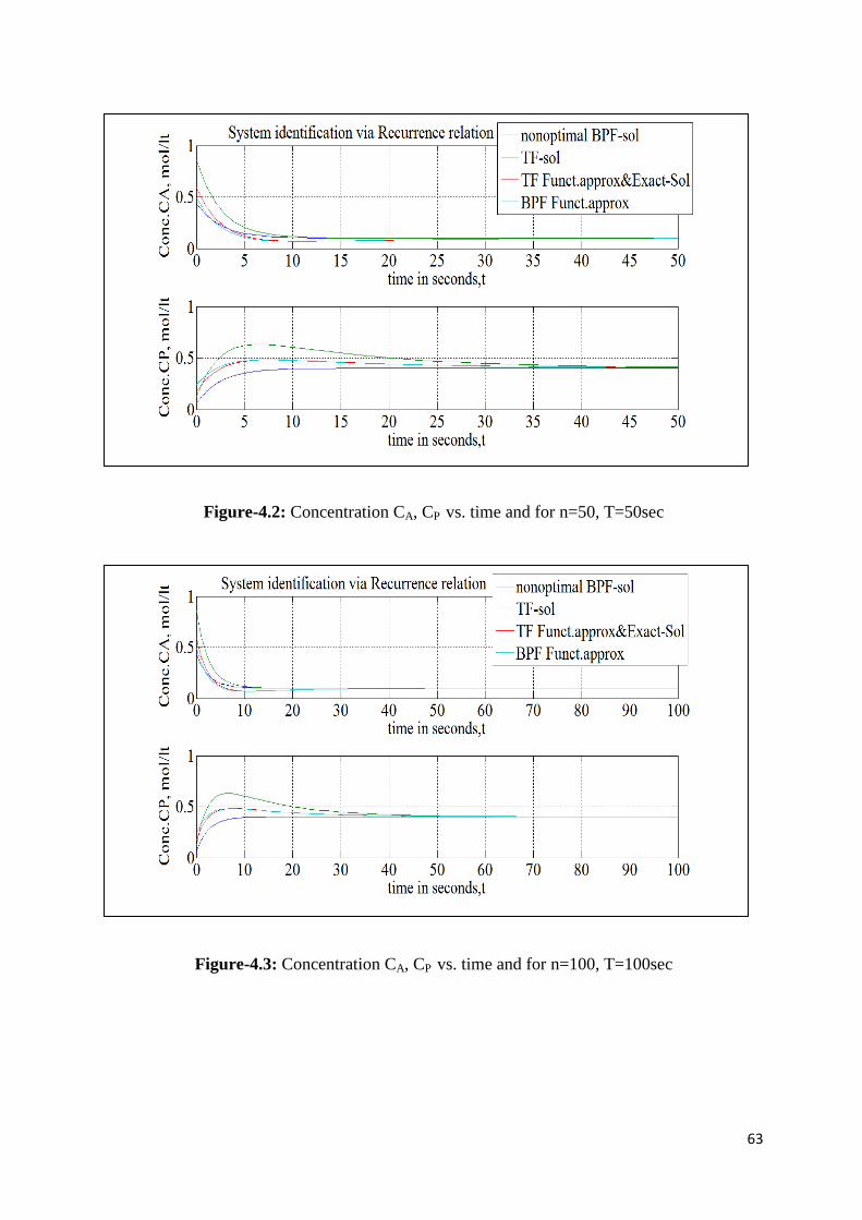
63
Figure-4.2: Concentration CA, CP vs. time and for n=50, T=50sec
Figure-4.3: Concentration CA, CP vs. time and for n=100, T=100sec

64
Table 4.1:- Results Comparison Table
T(sec) m(size) x1BPF x2BPF x1TF x2TF y1BPF y2BPF y1TF y2TF
10 10 0.1066 0.3936 0.1148 0.6065 0.0705 0.4676 0.071 0.4784
50 50 0.1001 0.4003 0.1001 0.4101 0.0988 0.407 0.098 0.4071
100 100 0.1001 0.4003 0.1001 0.4005 0.1006 0.4034 0.1006 0.4034
4.2) Simulation of a SISO system
Consider a linear time invariant SISO system whose model equations are given below
Model Equations:-
𝒅𝒙𝟏
𝒅𝒕= 𝒙𝟐. . . . . . . . . . . . . . . . . . . … … … … … … … … … … … … … … … … … … … . … … . . . . . . . . . . . (𝟒. 𝟑𝟎)
𝒅𝒙𝟐
𝒅𝒕= −𝟐𝒙𝟏 − 𝟑𝒙𝟐 + 𝟏. . . . . . . . . . . . . . . . . . . . . . . . . . . … … … … … … … … … … … . . . . . . . . . . . . (𝟒. 𝟑𝟏)
Expressing the above model equations in terms of state space matrices, we get
𝐴 = [
0 1−2 − 3
]; 𝑥0 = [01
]; 𝐸 = [00
]
For a given matrix size m and for a given time interval t the matrices A, x0 and E are
substituted in the recurrence relation to obtain the state vector coefficient in TF domain and
non-optimal BPF domain: Now the obtained output variables are compared over the variables
obtained using actual solution, function approximation using BPF and TF domains.
The actual solution of the system is obtained as:
𝒙𝟏(𝒕) = −𝒆−𝒕 + 𝟎. 𝟓𝒆−𝟐𝒕 + 𝟎. 𝟓 … … … … … … … … … … … … … … … … … … … … . … … … (𝟒. 𝟑𝟐)
𝒙𝟐(𝒕) = 𝒆−𝒕 − 𝒆−𝟐𝒕 … … … … … … … … … … … … … … … … … … … … … . … … … … … … … . (𝟒. 𝟑𝟑)
The function approximations using BPF and TF domain are calculated using equations (4.28)
and (4.29).The results are plotted using MATLAB against various time intervals, t=10, 20 and
30sec for various matrix sizes, m= 100 as shown below:
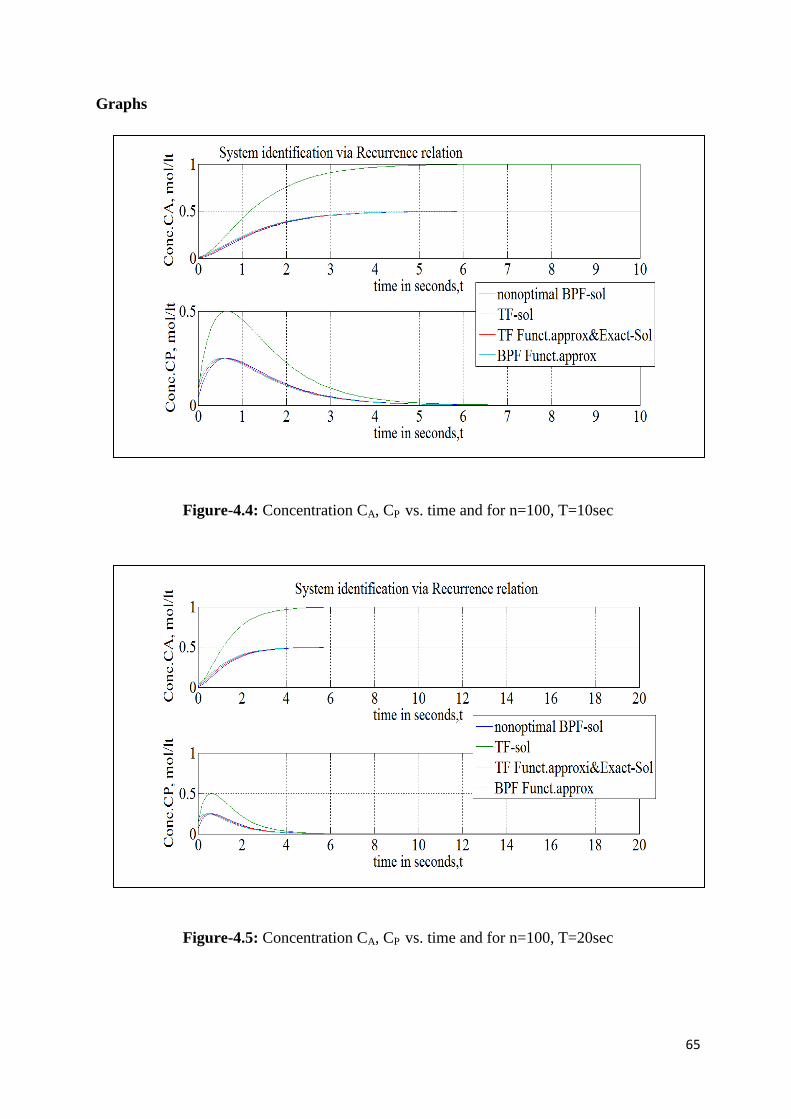
65
Graphs
Figure-4.4: Concentration CA, CP vs. time and for n=100, T=10sec
Figure-4.5: Concentration CA, CP vs. time and for n=100, T=20sec
66
Figure-4.6: Concentration CA, CP vs. time and for n=100, T=30sec
Table 4.2:- Results Comparison Table
T(sec) m(size) x1BPF x2BPF x1TF x2TF y1BPF y2BPF y1TF y2TF
10 100 0.5 0 0.9999 0.0001 0.5 0 0.5 0
20 100 0.5 05 1 0 0.5 0 0.5 0
30 100 0.5 0.5 1 0 0.5 0 0.5 0
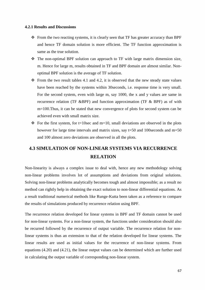
67
4.2.1 Results and Discussions
From the two reacting systems, it is clearly seen that TF has greater accuracy than BPF
and hence TF domain solution is more efficient. The TF function approximation is
same as the true solution.
The non-optimal BPF solution can approach to TF with large matrix dimension size,
m. Hence for large m, results obtained in TF and BPF domain are almost similar. Non-
optimal BPF solution is the average of TF solution.
From the two result tables 4.1 and 4.2, it is observed that the new steady state values
have been reached by the systems within 30seconds, i.e. response time is very small.
For the second system, even with large m, say 1000, the x and y values are same in
recurrence relation (TF &BPF) and function approximation (TF & BPF) as of with
m=100.Thus, it can be stated that new convergence of plots for second system can be
achieved even with small matrix size.
For the first system, for t=10sec and m=10, small deviations are observed in the plots
however for large time intervals and matrix sizes, say t=50 and 100seconds and m=50
and 100 almost zero deviations are observed in all the plots.
4.3 SIMULATION OF NON-LINEAR SYSTEMS VIA RECURRENCE
RELATION
Non-linearity is always a complex issue to deal with, hence any new methodology solving
non-linear problems involves lot of assumptions and deviations from original solutions.
Solving non-linear problems analytically becomes tough and almost impossible; as a result no
method can rightly help in obtaining the exact solution to non-linear differential equations. As
a result traditional numerical methods like Runge-Kutta been taken as a reference to compare
the results of simulations produced by recurrence relation using BPF.
The recurrence relation developed for linear systems in BPF and TF domain cannot be used
for non-linear systems. For a non-linear system, the functions under consideration should also
be recurred followed by the recurrence of output variable. The recurrence relation for non-
linear systems is thus an extension to that of the relation developed for linear systems. The
linear results are used as initial values for the recurrence of non-linear systems. From
equations (4.20) and (4.21), the linear output values can be determined which are further used
in calculating the output variable of corresponding non-linear system.
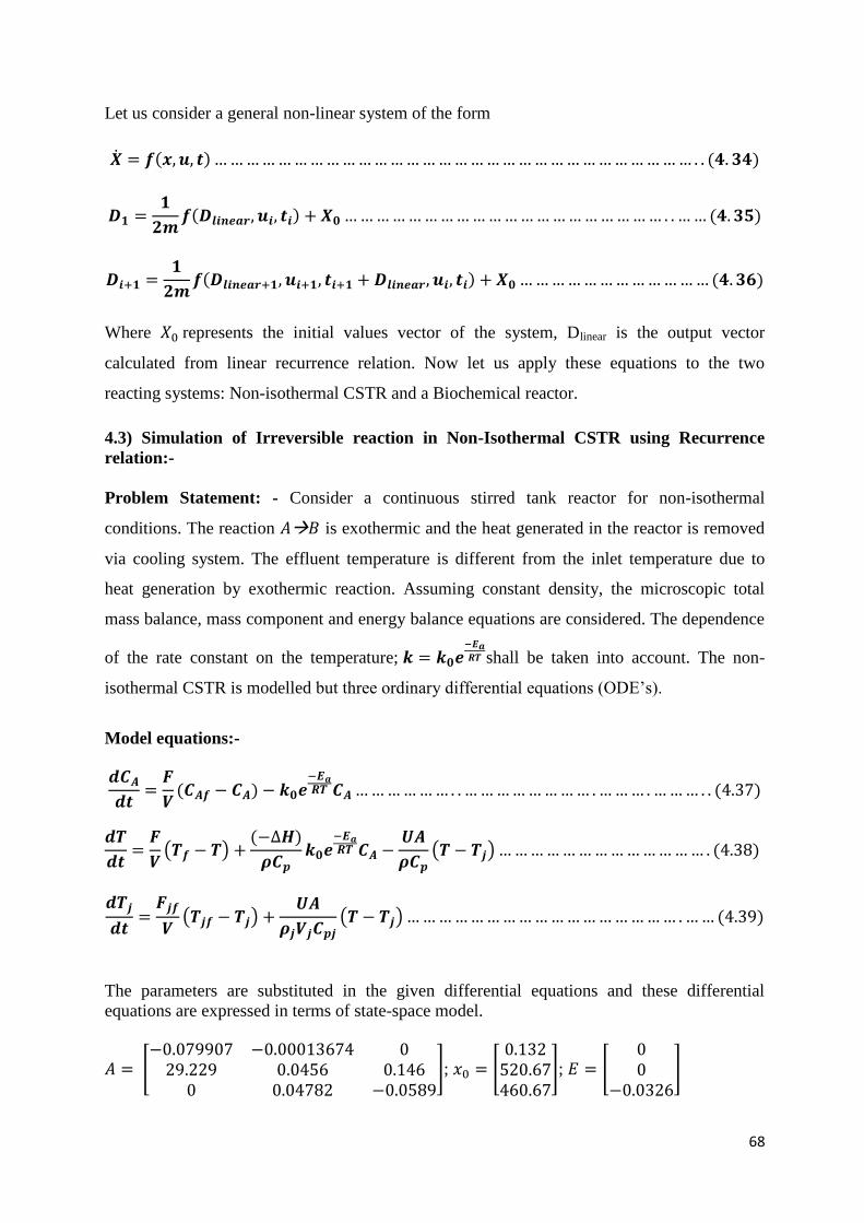
68
Let us consider a general non-linear system of the form
�̇� = 𝒇(𝒙, 𝒖, 𝒕) … … … … … … … … … … … … … … … … … … … … … … … … … … … … … … . . (𝟒. 𝟑𝟒)
𝑫𝟏 =𝟏
𝟐𝒎𝒇(𝑫𝒍𝒊𝒏𝒆𝒂𝒓, 𝒖𝒊, 𝒕𝒊) + 𝑿𝟎 … … … … … … … … … … … … … … … … … … … … . . … … (𝟒. 𝟑𝟓)
𝑫𝒊+𝟏 =𝟏
𝟐𝒎𝒇(𝑫𝒍𝒊𝒏𝒆𝒂𝒓+𝟏, 𝒖𝒊+𝟏, 𝒕𝒊+𝟏 + 𝑫𝒍𝒊𝒏𝒆𝒂𝒓, 𝒖𝒊, 𝒕𝒊) + 𝑿𝟎 … … … … … … … … … … … … (𝟒. 𝟑𝟔)
Where 𝑋0 represents the initial values vector of the system, Dlinear is the output vector
calculated from linear recurrence relation. Now let us apply these equations to the two
reacting systems: Non-isothermal CSTR and a Biochemical reactor.
4.3) Simulation of Irreversible reaction in Non-Isothermal CSTR using Recurrence
relation:-
Problem Statement: - Consider a continuous stirred tank reactor for non-isothermal
conditions. The reaction 𝐴𝐵 is exothermic and the heat generated in the reactor is removed
via cooling system. The effluent temperature is different from the inlet temperature due to
heat generation by exothermic reaction. Assuming constant density, the microscopic total
mass balance, mass component and energy balance equations are considered. The dependence
of the rate constant on the temperature; 𝒌 = 𝒌𝟎𝒆−𝑬𝒂𝑹𝑻 shall be taken into account. The non-
isothermal CSTR is modelled but three ordinary differential equations (ODE’s).
Model equations:-
𝒅𝑪𝑨
𝒅𝒕=
𝑭
𝑽(𝑪𝑨𝒇 − 𝑪𝑨) − 𝒌𝟎𝒆
−𝑬𝒂𝑹𝑻 𝑪𝑨 … … … … … … . . … … … … … … … … . … … … . … … … . . (4.37)
𝒅𝑻
𝒅𝒕=
𝑭
𝑽(𝑻𝒇 − 𝑻) +
(−∆𝑯)
𝝆𝑪𝒑𝒌𝟎𝒆
−𝑬𝒂𝑹𝑻 𝑪𝑨 −
𝑼𝑨
𝝆𝑪𝒑(𝑻 − 𝑻𝒋) … … … … … … … … … … … … … . (4.38)
𝒅𝑻𝒋
𝒅𝒕=
𝑭𝒋𝒇
𝑽(𝑻𝒋𝒇 − 𝑻𝒋) +
𝑼𝑨
𝝆𝒋𝑽𝒋𝑪𝒑𝒋(𝑻 − 𝑻𝒋) … … … … … … … … … … … … … … … … … . … … (4.39)
The parameters are substituted in the given differential equations and these differential
equations are expressed in terms of state-space model.
𝐴 = [−0.079907 −0.00013674 0
29.229 0.0456 0.1460 0.04782 −0.0589
]; 𝑥0 = [0.132
520.67460.67
]; 𝐸 = [00
−0.0326]

69
For a given matrix size m and for a given time interval t the matrices A, x0 and E are
substituted in the recurrence relation equations (4.34),(4.35) and (4.36) to obtain the state
vector coefficient in BPF domain. Now the obtained output variables are compared over the
outputs obtained using Runge-Kutta method.
The results are plotted using MATLAB against various time intervals, t=50, 100and 500 sec
for various matrix sizes, m=1, 2 and5 for 30 iterations as shown below:
Graphs
Figure-4.7: Concentration CA, T and Tj vs. time and for m=2, T=50sec
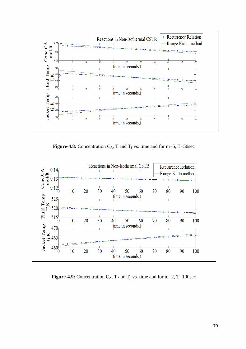
70
Figure-4.8: Concentration CA, T and Tj vs. time and for m=5, T=50sec
Figure-4.9: Concentration CA, T and Tj vs. time and for m=2, T=100sec
71
Figure-4.10: Concentration CA, T and Tj vs. time and for m=1, T=500sec
Another non-linear system which is simulated using the recurrence form is the biochemical
reactor in which bold glucose concentration is determined for the corresponding insulin
injected with the body. The system described previously in problem (3.5) is considered. Those
differential equations are multiplied by 0.01.The parameters are substituted in the differential
equations of problem (3.5) and these differential equations are expressed in terms of state-
space model.
𝐴 = 0.01 ∗ [−16.667 −4.5 029.229 −0.025 0.000013
0 0 −0.0926]; 𝑥0 = [
4.516.667
4.5]; 𝐸 = [
001
12
]
For a given matrix size m and for a given time interval t the matrices A, x0 and E are
substituted in the recurrence relation equations (4.34), (4.35) and (4.36) to obtain the state
vector coefficient in BPF domain. Now the obtained output variables are compared over the
outputs obtained using Runge-Kutta method.
The results are plotted using MATLAB against various time intervals, t=10, 20and 30 sec for
various matrix sizes, m=2 for 30 iterations as shown below:
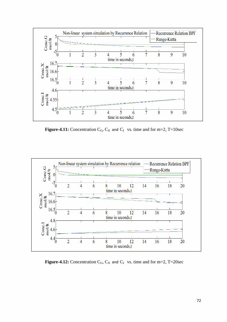
72
Figure-4.11: Concentration CG, CX and CI vs. time and for m=2, T=10sec
Figure-4.12: Concentration CG, CX and CI vs. time and for m=2, T=20sec
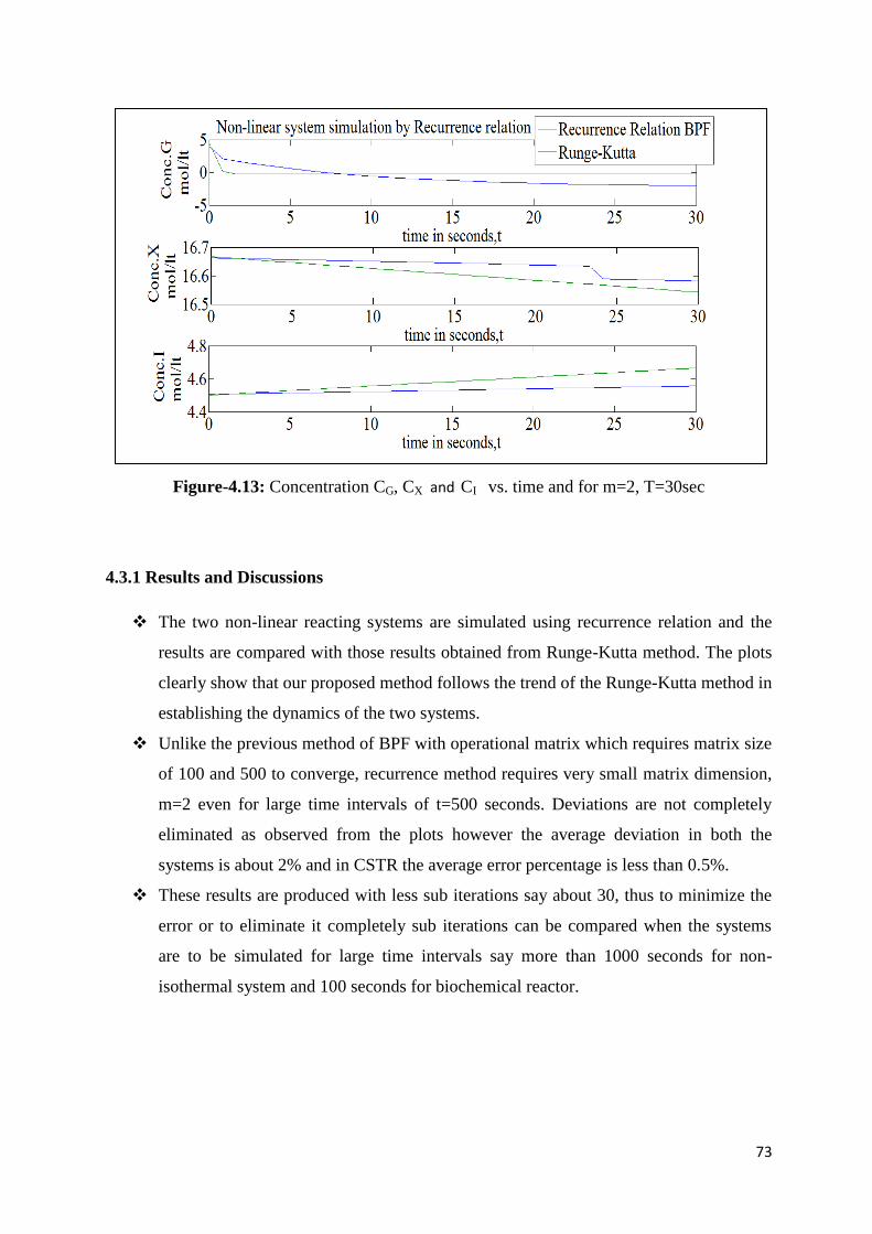
73
Figure-4.13: Concentration CG, CX and CI vs. time and for m=2, T=30sec
4.3.1 Results and Discussions
The two non-linear reacting systems are simulated using recurrence relation and the
results are compared with those results obtained from Runge-Kutta method. The plots
clearly show that our proposed method follows the trend of the Runge-Kutta method in
establishing the dynamics of the two systems.
Unlike the previous method of BPF with operational matrix which requires matrix size
of 100 and 500 to converge, recurrence method requires very small matrix dimension,
m=2 even for large time intervals of t=500 seconds. Deviations are not completely
eliminated as observed from the plots however the average deviation in both the
systems is about 2% and in CSTR the average error percentage is less than 0.5%.
These results are produced with less sub iterations say about 30, thus to minimize the
error or to eliminate it completely sub iterations can be compared when the systems
are to be simulated for large time intervals say more than 1000 seconds for non-
isothermal system and 100 seconds for biochemical reactor.
74
CHAPTER-5
OPTIMAL CONTROL OF CSTR’S USING
ORTHOGONAL FUNCTIONS
75
5.1 OPTIMAL CONTROL OF SYSTEMS
The basis for conventional control theory is the input-output relationship or transfer function.
On a contrary, the modern control theory is based on vector-matrix differential equation that
simplifies the mathematical representation of equations to a large extent. Even though the
number of states, inputs and outputs get increased, the complexity of the system does not get
increased. There had been several numerical techniques adopted earlier to obtain the states
and outputs by solving the matrices in state-space representation. Some of those methods are
recursive while some are non-recursive. Now, the block pulse functions are employed to
determine the optimality criterion and states of the system. The recursive computation derived
from block pulse functions is used in this regard.
Pole Placement method can determine the states only when all states are measurable, i.e. when
the system is completely controllable. In practise, not all states are completely measurable;
hence states estimation is not possible by pole placement method. By incorporating observers
within the system all states can be estimated.
Consider a linear time invariant completely observable and controllable system described by
�̇�(𝒕) = 𝑨𝒙(𝒕) + 𝑩𝒖(𝒕) … … … … … … … … … … … … … … … … … … … … … … … … … . … … . (𝟓. 𝟏)
𝒚(𝒕) = 𝑪𝒙(𝒕) … … … … … … … … … … … … … … … … … … … … … … . . … … … … … … . … … . . (𝟓. 𝟐)
Where u (t), x (t) and y (t) are plant input, state and output vectors respectively and A, B, C
are n×n, n×r and p×n real constant matrices respectively. Assume that the rank of C is p.
An observer described by
�̇�(𝒕) = 𝑭𝒛(𝒕) + 𝑮𝒖(𝒕) + 𝑯𝒚(𝒕) … … … … … … … … … … … … … … . . … … … … … … … … … . (𝟓. 𝟑)
�̂�(𝒕) = 𝑳𝟏𝒚(𝒕) + 𝑳𝟐𝒛(𝒕) … … … … … … … … … … … … … … … … … … … … … . … … … … … … (𝟓. 𝟒)
Can provide the estimate �̂�(𝑡) for the stare x (t), where F, G, H, L1, L2 are real constant q×q,
q×r, q×p, n×p and n×q matrices respectively and q=n-p when the following conditions are
satisfied.
𝐺 = 𝓣𝑩 … … … … … … … … … … … … … … … … … … … … … … … … … … … … . … … … … … … (𝟓. 𝟓)
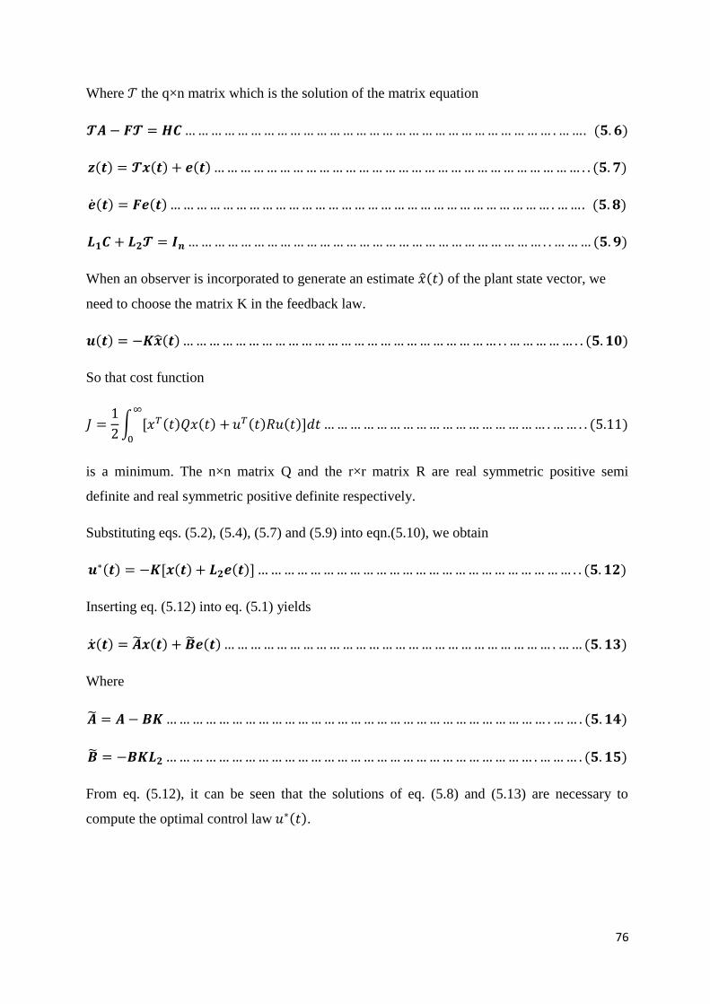
76
Where 𝒯 the q×n matrix which is the solution of the matrix equation
𝓣𝑨 − 𝑭𝓣 = 𝑯𝑪 … … … … … … … … … … … … … … … … … … … … … … … … … … … … . … …. (𝟓. 𝟔)
𝒛(𝒕) = 𝓣𝒙(𝒕) + 𝒆(𝒕) … … … … … … … … … … … … … … … … … … … … … … … … … … … … . . (𝟓. 𝟕)
�̇�(𝒕) = 𝑭𝒆(𝒕) … … … … … … … … … … … … … … … … … … … … … … … … … … … … … . … …. (𝟓. 𝟖)
𝑳𝟏𝑪 + 𝑳𝟐𝓣 = 𝑰𝒏 … … … … … … … … … … … … … … … … … … … … … … … … … … … . . … … … (𝟓. 𝟗)
When an observer is incorporated to generate an estimate �̂�(𝑡) of the plant state vector, we
need to choose the matrix K in the feedback law.
𝒖(𝒕) = −𝑲𝒙(𝒕) … … … … … … … … … … … … … … … … … … … … … … … … . . … … … … … . . (𝟓. 𝟏𝟎)
So that cost function
𝐽 =1
2∫ [𝑥𝑇(𝑡)𝑄𝑥(𝑡) +
∞
0
𝑢𝑇(𝑡)𝑅𝑢(𝑡)]𝑑𝑡 … … … … … … … … … … … … … … … … … . … … . . (5.11)
is a minimum. The n×n matrix Q and the r×r matrix R are real symmetric positive semi
definite and real symmetric positive definite respectively.
Substituting eqs. (5.2), (5.4), (5.7) and (5.9) into eqn.(5.10), we obtain
𝒖∗(𝒕) = −𝑲[𝒙(𝒕) + 𝑳𝟐𝒆(𝒕)] … … … … … … … … … … … … … … … … … … … … … … … … . . (𝟓. 𝟏𝟐)
Inserting eq. (5.12) into eq. (5.1) yields
�̇�(𝒕) = �̃�𝒙(𝒕) + �̃�𝒆(𝒕) … … … … … … … … … … … … … … … … … … … … … … … … … . … … (𝟓. 𝟏𝟑)
Where
�̃� = 𝑨 − 𝑩𝑲 … … … … … … … … … … … … … … … … … … … … … … … … … … … … … . … … . (𝟓. 𝟏𝟒)
�̃� = −𝑩𝑲𝑳𝟐 … … … … … … … … … … … … … … … … … … … … … … … … … … … … . … … … . (𝟓. 𝟏𝟓)
From eq. (5.12), it can be seen that the solutions of eq. (5.8) and (5.13) are necessary to
compute the optimal control law 𝑢∗(𝑡).
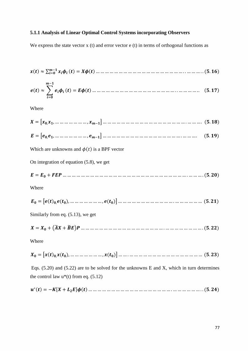
77
5.1.1 Analysis of Linear Optimal Control Systems incorporating Observers
We express the state vector x (t) and error vector e (t) in terms of orthogonal functions as
𝒙(𝒕) ≈ ∑ 𝒙𝒊𝝓𝒊𝒎−𝟏𝒊=𝟎 (𝒕) = 𝑿𝝓(𝒕) … … … … … … … … … … … … … … … … … … … . . … … … . . (𝟓. 𝟏𝟔)
𝒆(𝒕) ≈ ∑ 𝒆𝒊𝝓𝒊
𝒎−𝟏
𝒊=𝟎
(𝒕) = 𝑬𝝓(𝒕) … … … … … … … … … … … … … … … … … … . . … … … … .. (𝟓. 𝟏𝟕)
Where
𝑿 = [𝒙𝟎,𝒙𝟏, … … … … … … … , 𝒙𝒎−𝟏] … … … … … … … … … … … … … … … … … … . … … …. (𝟓. 𝟏𝟖)
𝑬 = [𝒆𝟎,𝒆𝟏, … … … … … … … , 𝒆𝒎−𝟏] … … … … … … … … … … … … … … … … … . … … …. (𝟓. 𝟏𝟗)
Which are unknowns and 𝜙(𝑡) is a BPF vector
On integration of equation (5.8), we get
𝑬 = 𝑬𝟎 + 𝑭𝑬𝑷 … … … … … … … … … … … … … … … … … … … … … … … … … … … . … … … . (𝟓. 𝟐𝟎)
Where
𝑬𝟎 = [𝒆(𝒕)𝟎,𝒆(𝒕𝟎), … … … … … … … , 𝒆(𝒕𝟎)] … … … … … … … … … … … … . … … … … … … (𝟓. 𝟐𝟏)
Similarly from eq. (5.13), we get
𝑿 = 𝑿𝟎 + (�̃�𝑿 + �̃�𝑬)𝑷 … … … … … … … … … … … … … … … … … … . … … … … … … … … . (𝟓. 𝟐𝟐)
Where
𝑿𝟎 = [𝒙(𝒕)𝟎,𝒙(𝒕𝟎), … … … … … … … , 𝒙(𝒕𝟎)] … … . … … … … … … … … … … … … … … … … (𝟓. 𝟐𝟑)
Eqs. (5.20) and (5.22) are to be solved for the unknowns E and X, which in turn determines
the control law u*(t) from eq. (5.12)
𝒖∗(𝒕) = −𝑲[𝑿 + 𝑳𝟐𝑬]𝝓(𝒕) … … … … … … … … … … … … … … … … … … . … … … … … … . . (𝟓. 𝟐𝟒)
78
Now the eqs. (5.20) and (5.22) are solved by a recursive algorithm via BPF’s
Substituting the operational matrix P in eqs, (5.20) and (5.22) and simplifying we obtain
𝒆𝟎 = (𝑰𝒒 − 𝟎. 𝟓𝑻𝑭)−𝟏
𝒆(𝒕𝟎) … … … … … … … … … … … … … … … … … … … . … … … … … . . (𝟓. 𝟐𝟓)
𝒆𝟏 = (𝑰𝒒 − 𝟎. 𝟓𝑻𝑭)−𝟏
(𝑰𝒒 + 𝟎. 𝟓𝑻𝑭)𝒆𝒊−𝟏 … … … … … … … … … … … … . … … … … … … . . (𝟓. 𝟐𝟔)
For i=1, 2, 3…, m-1
𝒙𝟎 = (𝑰𝒏 − 𝟎. 𝟓𝑻�̃�)−𝟏
[𝒙(𝒕𝟎) + 𝟎. 𝟓𝑻�̃�𝒆𝟎] … … … … … … … … … … … … . … … … … . … .. (𝟓. 𝟐𝟕)
𝒙𝒊 = (𝑰𝒏 − 𝟎. 𝟓𝑻�̃�)−𝟏
[(𝑰𝒏 + 𝟎. 𝟓𝑻�̃�)𝒙(𝒕𝟎) + 𝟎. 𝟓𝑻�̃�(𝒆𝒊−𝟏 + 𝒆𝒊)] … … … … … . . … … . . (𝟓. 𝟐𝟖)
For i=1, 2, 3…, m-1
Problem Statement: - Consider a linear time-invariant system which is represented by the
state space matrices given in the following
[�̇�1(𝑡)�̇�2(𝑡)
] = [0 11 0
] [𝑥1(𝑡)𝑥2(𝑡)
] + [0
−1] 𝑢(𝑡)
[𝑥1(0)𝑥2(0)
] = [−0.60.35
]
𝑦(𝑡) = [1 0][𝑥1(𝑡) 𝑥2(𝑡)]𝑇
Where the optimal control law can be taken to be
𝑢∗(𝑡) = −𝐾�̂�(𝑡) = [1.5 1][�̂�1(𝑡) �̂�2(𝑡)]𝑇
There is no complete measurement of state, hence �̂�(𝑡) can be obtained by the Luenberger
observer. Let us choose
𝐿1 = [1 1.5]𝑇 and 𝐿2 = [0 1]𝑇
Substituting L1 and L2 in eq. (5.4) we get
[�̂�1(𝑡)�̂�2(𝑡)
] = [1
1.5] 𝑦(𝑡) + [
01
] 𝑧(𝑡)
𝒯 is determined from eq. (5.9) , G is known from eq. (5.5) and F,H are known from eq. (5.6).
The obtained F, G and H values are substituted in eq. (5.3)

79
�̇�(𝑡) = −1.5𝑧(𝑡) − 𝑢(𝑡) − 1.25𝐻𝑦(𝑡) … … … … … … … … … … … . . … … . … . … … … … … . (5.29)
𝐴 = [0 11 0
] ; 𝐵 = [0
−1] ; 𝐶 = [1 0]; 𝐾 = [1.5 1]; 𝐹 = −1.5; 𝐺 = −1; 𝐻 = −1.25;
𝐿1 = [1
1.5] ; 𝐿2 = [
01
]; 𝒯 = [−1.5 1]
�̃� = 𝐴 − 𝐵𝐾 = [0 1
−0.5 −1] and �̃� = −𝐵𝐾𝐿2
Substituting F in eqs. (5.25) and (5.26) to compute error vector. Similarly �̃� and �̃� are
substituted in recursive algorithm in eqs. (5.27) and (5.28) to compute state vector. Therefore,
for m=4 and 9, the states and error vector is computed from the recurrence relation via BPF’s.
The results are plotted against different time intervals and compared with the plots of the true
solutions.
Graphs
Figure 5.1: Error versus time, t=10sec, m=4
80
Figure 5.2: State variables versus time, t=10sec
Figure 5.3: Error versus time, t=10sec, m=9
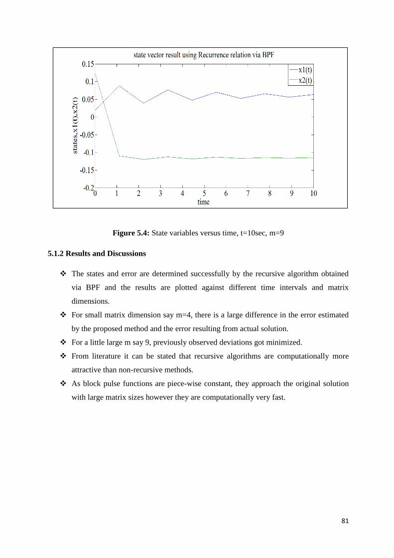
81
Figure 5.4: State variables versus time, t=10sec, m=9
5.1.2 Results and Discussions
The states and error are determined successfully by the recursive algorithm obtained
via BPF and the results are plotted against different time intervals and matrix
dimensions.
For small matrix dimension say m=4, there is a large difference in the error estimated
by the proposed method and the error resulting from actual solution.
For a little large m say 9, previously observed deviations got minimized.
From literature it can be stated that recursive algorithms are computationally more
attractive than non-recursive methods.
As block pulse functions are piece-wise constant, they approach the original solution
with large matrix sizes however they are computationally very fast.
82
CHAPTER-6
CONCLUSIONS AND FUTURE SCOPE
83
CONCLUSION
BPF with an operational matrix, P is an efficient method in simulating the differential
equations of linear reacting systems.
However they are not that efficient in simulating all the non-linear systems. Non-linear
differential equations with exponential terms in them are difficult to be solved by this
method.
Recurrence relation in BPF and TF domain is proved to be effective in solving all the
linear system of differential equations.
Recurrence relation in BPF domain can successfully solve non-linear CSTR system.
Optimality criterion for control problems can be achieved by recursive algorithms via
BPF and also the states, input and error can be determined.
FUTURE SCOPE
Block pulse functions can be applied to Heat exchangers, distillation processes and
coal plant simulations. In addition, the other important orthogonal functions like
triangular function sets with operational matrices can be applied to these processes.
The recurrence relation using triangular functions can be developed and implemented
on the processes.
System identification, parameter estimation and control are the important phenomena
of system analysis. As system identification has been worked upon, parameter
estimation of chemical processes can be worked in the future.

84
REFERENCES
1) A. Ganti Prasad Rao, “Piecewise Constant Orthogonal Functions and their Application
to System and Control,” Springer-Verlag (1983).
2) A.Deb, G .Sarkar and S.K. Sen (1994),”Block pulse functions, the most fundamental
of all piecewise constant basis functions,” Int. J. Syst. Sci., 25(2), 351-363.
3) Beauchamp K.G, “Applications of Walsh and Related Functions with an Introduction
to Sequency theory,” Academic Press, London, 1984.
4) C.F.Chen, Y.T.Tsay and T.T.Wu, “Walsh operational matrices for fractional calculus
and their applications to distributed systems”, Journal- The Franklin Institute, vol.303,
no.3, pp:267-284, (1977)
5) C.Hwang, D.H.Shih and F.C.Kung, “Use of Block-pulse functions in optimal control
of deterministic systems”, International Journal of Control, vol.44, no.2, pp: 613-
624,(1986).
6) C.T Liou and Y.S Chou, “Piecewise linear polynomial functions and their applications
to analysis and parameter identification,” International Journal of Systems and
Science, vol.18, no. 10, pp.1919-1929, (1987).
7) D.Leunberger, “Observing the state of a linear system,” IEEE Trans. on Military
electronics,vol.8,pp:74-80,1964
8) E. Babolian and Z. Masouri, “Direct method to solve Volterra integral equation of the
first kind using operational matrix with block-pulse functions”, Applied Mathematics
and Computation, 220 (2008) 51-57.
9) E. Coddington and N. Levinson, “Theory of Ordinary Differential Equations”,
McGraw Hill, New York, (1955).
10) E. Hashemizadeh, K. Maleknejad and M.R.Mohsenyzadeh, “Hybrid Orthonormal
Bernstein and Block-Pulse Functions for Solving Fredholm Integral Equations”,
Proceedings of the World Congress on Engineering 2013 Vol I, WCE(2013), London,
U.K.
11) G. Birkhoff and G. Rota, “Ordinary Differential Equations”, Blaisdell, Waltham,
(1969).
12) G. Froment, and K.B Biscoff, “Chemical Reactor Analysis and Design”, John Wiley
&sons, 2nd Edition, New York (1990).
13) G.P.Rao., L Sivakumar. (1978) “Analysis and synthesis of dynamic systems
containing time-delays via block-pulse functions,” Proc. IEE, 125, 1064-1068.
14) H. Khalil, “Nonlinear Systems”, Macmillan, (1992).

85
15) H.R. Marzban., M. Razzaghi, (2004), “Optimal control of linear delay systems via
hybrid of block-pulse and Legendre polynomials,” J. Franklin Inst., 341, 279-293.
16) I.S.MetCalfe, “Chemical Reaction Engineering”, Oxford University Press Oxford UK
(1997).
17) J.h.Chou and I.R.Horng, “Shifted Legendre series analysis of linear optimal control
systems incorporating observers”, International Journal of Systems and Science,
vol.16, no.7, pp: 863-867,(1985).
18) J.H.Park, Korea National University of Transportation, Republic of Korea, “Trajectory
Optimization for Large Scale Systems via Block Pulse Functions and
Transformations”, International Journal of Control and Automation Vol. 5, No. 4,
December, (2012).
19) K. Maleknejad and K. Mahdiani ,”Iterated Block-Pulse Method for Solving Volterra
Integral Equations”, Applied Mathematics (2012), 2(1): 17-20
20) K. Ogata, Modern control engineering (4th
ed.), Pearson Education Asia, New Delhi,
2002.
21) K.B.Datta and B.M.Mohan, “Orthogonal Functions in Systems and Control”,
Advanced Series in Electrical and Computer Engineering, vol.9, World Scientific,
Singapore, (1995).
22) M. Vidyasagar, “Nonlinear Systems Analysis”, Prentice Hall, 2nd Edition (1992).
23) M.Razzaghi, H.R. Marzban (2000) “Direct method for variational problems via hybrid
of block-pulse and Chebyshev functions,” Math. Probl. Eng., 6, 85-97.
24) N.K.Sinha and Z.Q.Jie, “State estimation using block pulse functions”, International
Journal of Systems and Science, vol.15,no.4,pp:341-350,(1984)
25) P. Sannuti “Analysis and Synthesis of dynamic systems containing time delays via
block pulse functions,” Proc.IEE, vol.125, no.9, pp.1064-1068,(1978).
26) P. Sannuti “Analysis and synthesis of dynamic systems via block-pulse functions,”
Proc. Inst. Electr. Eng., 124, 569-571, (1977).
27) P. Schiavane, C. Constanda, A. Mioduchowski’ (2002); “Integral Methods in Science
and Engineering’’, Birk¨auser, Boston.
28) R. Cole, “Theory of Ordinary Differential Equations” Appleton-Century- Crofts, New
York, (1968).
29) T.T.Lee, S.C.Tsay and I.R.Horng, “Shifted Jacobi series analysis of linear optimal
control systems incorporating observers”, Journal The Franklin Institute, vol.321, no.5,
pp: 289-298,(1986).

86
30) Z.h.Ziang and W.Schaufelberger, “Block pulse functions and their Applications in
Control Systems”, LNCIS 179, Springer, Berlin,(1992).


![[MartiÌ-n, Montes, Galan, 2008] Bubbling process in stirred tank reactors II - Agitator effect on the mass transfer rates.pdf](https://img.pdfslide.net/doc/110x75/55cf91e8550346f57b91aac1/martii-n-montes-galan-2008-bubbling-process-in-stirred-tank-reactors-56115c7e0e937.jpg)