Labelling Method by Pupillometry for Classifying Attention

九州大学学術情報リポジトリKyushu University Institutional Repository

Labelling Method by Pupillometry forClassifying Attention Level by EEG/ECG/NIRS

ゼニファ, ファディラ

https://doi.org/10.15017/4060012

出版情報：九州大学, 2019, 博士（システム生命科学）, 課程博士バージョン：権利関係：

Labelling Method by Pupillometry for Classifying

Attention Level by EEG-ECG-NIRS

Fadilla Zennifa

Graduate School of Systems Life Sciences

Kyushu University

2020

2

Abstract

There are numerous methods to evaluate attention levels such as observation, self-

assessment, and objective performance. This study aims to propose a new labeling method

for attention levels detection by using parameter settings of pupillometry. This parameter

setting then would be applied as data labeling in supervised machine learning toward EEG-

ECG-NIRS.

To develop parameter settings of attention level evaluation, this study investigated

the reaction of blink rates and pupillometry toward attention level based on self-assessment

during cognitive tasks. My result showed there is no significant differences (P>0.05) in blink

rates toward attention level within 10 seconds. On the other hand, pupillometry in low

attention showed significant differences in pupillometry in the last 4 seconds cognitive tasks

(P<0.05). After that, I calculated the distribution fit of pupillometry reaction in the attention

level of all participants and plot the critical point of pupillometry data in 10 seconds and 4

seconds. After doing several experimental procedures, I chose parameter setting with a

percentage of error of less than 15% and a different error 35 % compare with self assesment

as future labeling method. Parameter setting which has been selected is when z-score within

a specific range (-0.965 ≤ pupil ≤ 1.014) as high attention, other that range, will be classified

as low attention.

Furthermore, I applied my labeling method for another physiological signal such as

electroencephalograph (EEG), electrocardiograph (ECG), and near-infrared spectroscopy

(NIRS). Numerous methods using electroencephalograph (EEG), electrocardiograph (ECG),

and near-infrared spectroscopy (NIRS) for attention level detection have been proposed.

3

However, the results were either unsatisfactory or required many channels. In this study, I

introduce the implementation of an EEG-ECG-NIRS for attention level detection. I used two-

electrode wireless EEG, a wireless ECG, and two wireless channels NIRS to detect attention

level during backward digit span, forward digit span and arithmetic. High attention will be

labelled to data which has pupillometry z-score within specific range (-0.965 ≤ pupil ≤ 1.014)

and another that range, will be classified as low attention. By using CFS+kNN algorithm, my

result showed the accuracy system of EEG-ECG-NIRS (83.33± 5.95%) has the highest

accuracy compare with EEG (81.90± 4.69%), ECG (82.51±3.57%), NIRS (78.37±7.12%).

Algorithm CFS+kNN also shown highest performance compare with other methods such as

CFS+SVM (55.49± 27.89%), kNN (80.84± 3.88%) and SVM (55.88± 13.14%)

In summary, in this study, I established new parameter settings for evaluating

attention level by using pupillometry and apply the parameter settings into EEG-ECG-NIRS

to evaluate the EEG-ECG-NIRS performance, comparing with standalone system.

Keywords: labeling, supervised machine learning, blink rates, pupillometry,

electroencephalograph, electrocardiograph, near-infrared spectroscopy, attention level

detection

4

Ethics statement

The protocols for the present study were designed in accordance with the Declaration of

Helshinki and were approved by faculty of information science and electrical engineering,

Kyushu University (H26–3). Informed consent was obtained in writing from each participant

5

Table of Contents Abstract ............................................................................................................................................... 2

Ethics statement ................................................................................................................................ 4

Chapter 1. General Introduction ..................................................................................................... 7

1.1 Some basic notions ................................................................................................................. 10

1.1.1 Attention level detection. ............................................................................................... 10

1.1.2 Blink rates and Pupillometry ........................................................................................ 11

1.1.3 EEG, ECG, NIRS research toward attention .............................................................. 13

1.2 Thesis overview ...................................................................................................................... 14

1.3 Purpose of this study .............................................................................................................. 15

Chapter 2. New Labelling method for attention level detection ................................................. 17

2.1 Abstract ................................................................................................................................... 17

2.2. Materials and Methods ......................................................................................................... 18

2.2.1 Participants ..................................................................................................................... 18

2.2.2 Experiment condition ..................................................................................................... 18

2.2.3. Software and Apparatus ............................................................................................... 19

2.3 Data Analysis .......................................................................................................................... 21

2.3.1 Comparison system from all attention level detection method .................................. 21

2.3.2 Blink rates and pupillometry analysis .......................................................................... 22

2.4 Results ..................................................................................................................................... 26

2.4.1 Self-assessment reliability for the basis on quantitative formula .............................. 27

2.4.2 Parameter settings for attention level ........................................................................... 33

2.4.3.The error rate of quantitative for attention level ........................................................ 44

2.5 Discussion ............................................................................................................................... 47

2.6 Conclusion ............................................................................................................................... 53

Chapter 3. Application of new labeling in EEG-ECG-NIRS ...................................................... 55

3.1. Abstract .................................................................................................................................. 55

3.2 Materials and method ............................................................................................................ 55

3.2.1 Participants ..................................................................................................................... 55

3.2.2 Experiment task.............................................................................................................. 56

3.2.3. Software and Apparatus ............................................................................................... 58

6

3.3 Analysis for New Labelling of Attention Level Detection in EEG-ECG-NIRS ......................... 60

3.3.1 Data Preprocessing ......................................................................................................... 61

3.3.2. Data Management ......................................................................................................... 73

3.4 Results ..................................................................................................................................... 77

3.4.1. EEG-ECG- NIRS toward Attention Level Based on Purposed Labelling Method . 77

3.4.2. Classification algorithm ................................................................................................ 78

3.5. Discussion .............................................................................................................................. 82

3.6. Conclusions ............................................................................................................................ 84

Chapter 4. General Discussion ....................................................................................................... 86

Acknowledgement ............................................................................................................................ 92

References ......................................................................................................................................... 93

Appendix 1. Consent to participate example for experiment chapter 2. ......................................... 111

Appendix 2. Consent to participate example for experiment chapter 3. ......................................... 114

Appendix 3. Experiment report summary for chapter 2. ................................................................. 117

Appendix 4. Experiment report summary for chapter 3. ................................................................. 121

Appendix 5. pupillometry activities based on tasks ........................................................................ 128

Appendix 6. Script program in this thesis. ...................................................................................... 142

Appendix 7. Supporting software in this thesis ............................................................................... 156

7

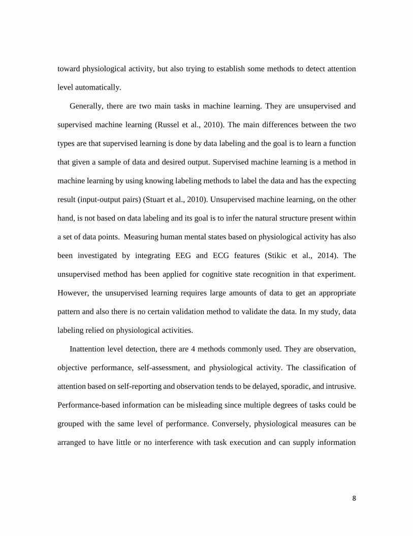
Chapter 1. General Introduction

Attention can be defined as the processing or selection of information at the expense of

other information (Phashler et al., 1998; Anderson et al., 2004; Fougnie. 2008). Similarly,

in 1890 psychologists and philosophers William James defines attention as taking possession

by the mind, in clear and vivid form, of one out of what may seem several simultaneously

possible objects or trains of thought. This implies withdrawal from some things to deal

effectively with others (James. 1890). Attention also has been a key cognitive mechanism of

interest in terms of differentiating among the various measures of time (Campbell et al.,

2015). Knowing the human attention level helps improve human working and study

efficiency (Berka et al., 2007; Sun et al., 2014). A study about attention in the psychology

field was introduced by Wilhelm Wundt (Titchener., 1921). In 1868, Franciscus Donders

investigated reaction time toward attention by using chronometry. Which the meaning of

chronometry is the study about temporal sequencing of information in the brain (Donders.

1969). In the 1990s, positron emission tomography (PET) is started to be used for attention

studies (Petersen et al., 1988; Posner and Petersen. 1990; Burton et al., 1999). In 1993,

Osman et al (Osman et al., 1993) mentioned that attention can also affect EEG signals

associated with later central processing stages, such as those involved in the selection and

initiation of responses. Research about attention also has been investigated by using

Electrocardiogram (ECG) (Borger et al., 1999; Smallwood et al., 2004; Griffiths et al., 2017).

Investigation of attention toward hemodynamic activity has been measured by using Near-

Infrared Spectroscopy (NIRS) (Matsuda and Hiraki. 2006; Toichi et al., 2004; Derosière et

al., 2013). Nowadays researchers are not only trying to investigate the effect of attention

8

toward physiological activity, but also trying to establish some methods to detect attention

level automatically.

Generally, there are two main tasks in machine learning. They are unsupervised and

supervised machine learning (Russel et al., 2010). The main differences between the two

types are that supervised learning is done by data labeling and the goal is to learn a function

that given a sample of data and desired output. Supervised machine learning is a method in

machine learning by using knowing labeling methods to label the data and has the expecting

result (input-output pairs) (Stuart et al., 2010). Unsupervised machine learning, on the other

hand, is not based on data labeling and its goal is to infer the natural structure present within

a set of data points. Measuring human mental states based on physiological activity has also

been investigated by integrating EEG and ECG features (Stikic et al., 2014). The

unsupervised method has been applied for cognitive state recognition in that experiment.

However, the unsupervised learning requires large amounts of data to get an appropriate

pattern and also there is no certain validation method to validate the data. In my study, data

labeling relied on physiological activities.

Inattention level detection, there are 4 methods commonly used. They are observation,

objective performance, self-assessment, and physiological activity. The classification of

attention based on self-reporting and observation tends to be delayed, sporadic, and intrusive.

Performance-based information can be misleading since multiple degrees of tasks could be

grouped with the same level of performance. Conversely, physiological measures can be

arranged to have little or no interference with task execution and can supply information

9

continuously without significant delay (Yurko et al., 2010; Sun et al., 2014; Aghajani et al.,

2017).

This study aims to label attention level using pupillometry, which can be further used in

a supervised machine learning system of attentional evaluation. In this thesis I focused on

how to establish the algorithm for new labeling by using pupillometry, after that, I applied

the label and established the model algorithm based on supervised machine learning on EEG-

ECG-NIRS for attention level detection.

As the task design, I used common attention task test which is digited span forward and

backward (Jensen et al., 1975; Cullum., 1998; Berka et al 2007, Zennifa et al., 2018; Zennifa

et al., 2019), and additionally, I also applied the arithmetic test (Zennifa et al., 2018; Zennifa

et al., 2019). Most of the questions in this experiment were relatively simple and did not

require any prerequisite knowledge or specific skills. However, a good level of attention and

alertness was required to avoid making easy mistakes. There were several problems need to

solve before taking the experiment. All participants had a normal visual function, were not

with a disability and could do the experiment without wearing glasses. I also asked

participants to have breakfast and not drink any caffeine before taking the test. Some

participants did not follow this rule, and we have to exclude their data.

I am currently implementing a parameter setting based on features of pupillometry and

for data labeling, I used Weka 3.8 (Hall et al., 2009) data mining for machine learning. I also

applied a CFS + KNN algorithm on an EEG-ECG-NIRS system and used a searching

algorithm which is called “best first”.

10

In the next section, I reviewed basic knowledge of attention level detection and blink

rates, pupillometry and also EEG-ECG-NIRS. Furthermore, I introduced the related literature

about attention level detection.

1.1 Some basic notions

1.1.1 Attention level detection.

Attention is the behavioral and cognitive process of selectively concentrating on a

discrete aspect of information, whether deemed subjective or objective while ignoring other

perceivable information. Knowing human attention is useful for efficiency in both working

and studying (Berka et al., 2007, Sun et al., 2014).

There are 178 journals and magazines about attention level detection in the current past

10 years based on IEEE explore. There are 16 articles about “attention level detection” based

on google scholars within 10 years. There are 139 journal articles about “attention

pupillometry” based on pubmed.gov. Attention level detection has been done (by D.Das et

al., 2013) in two classifications high attention and low attention based on behavioral pattern

analysis. They used a robot as an observer to captures the attention of the person. But this

research purely based on participant behavior. Another researcher (Sun et al., 2014), by using

facial expression try to detect the attention level which accuracy up to 77.81%. By using

facial expression is also depends on country culture. (Hussain et al., 2014) investigated the

activity of physiological signals and facial responses to cognitive load under an emotional

stimulus and collected participant ratings from a self-assessment manikin to find the

normative ratings in the collection. They investigated the correlation between physiological

data and the level of stimulation. They also subsequently compared the accuracy of cognitive

11

load detection with face video features, physiological features, and participant rating features

with fusion features. They concluded that classification with fusion features (i.e., not only

based on self-report) performed with more accuracy. In my study, I proposed to establish a

new labeling method for attention level detection and using the labeling data to train data

from EEG-ECG-NIRS.

1.1.2 Blink rates and Pupillometry

In this study, I used EOG (electrooculogram) to measure blink rates and eye tracker to

record pupillometry. EOG records eye movements by measuring electrical potential

differences between two electrodes. This takes advantage of the fact that the human eye is an

electrical dipole consisting of a positively charged cornea and a negatively charged retina,

first discovered by Schott in 1922 (Muller et al 2016). When I used EOG, blink specify by

amplitude more than 150 μV (Zennifa et al 2018.,; Bulling et al., 2011; Abo-zahhad et al.,

2015; He S., 2017). Blink rates are the number of blinks at specific times. Eyeblinks are

actively involved in the release of attention (Nakano et al, 2013). (Marc et al, 2015) evaluated

spontaneous eye blink rate (SEBR) and percentage of incomplete blinks in different hard-

copy and visual display terminal (VDT) reading conditions, compared with baseline

conditions. In that study, they concluded that high cognitive demands associated with a

reading task led to a reduction in SEBR, irrespective of the type of reading platform. However,

only electronic reading resulted in an increase in the percentage of incomplete blinks, which

may account for the symptoms experienced by VDT users. Blinking has been correlated with

cognitive activity (Paprocki et al., 2017). Their study mentioned that blink rate carry

information about cognitive performance and can be employed in the assessment of cognitive

12

abilities without taking a test. Blink rate for mental states is performed by (Ren et al., 2019)

in their paper, they attempted to differentiate between high and low cognitive loads of an

individual through the analyses of BR and BRV (blink rate variability). The result indicated

that BRV achieves significantly higher AUC values than BR, which suggests its strong

potentiality for MSR. In sum, the BRV may prove to be a promising method for the MSR,

which should be considered in the future.

Pupillometry is the measurement of pupil size and reactivity. It is also used in psychology

(Granholm et al., 2004). Pupillometry is concerned with changes in pupil size. The diameter

of the pupil size has long been known as a marker of cognitive load and attentional

performance (Karatekin et al., 2007; Tsukahara et al., 2016; Hartmann et al, 2014; Geva et

al., 2013; Unsworth et al., 2017 a&b; Piquado et al., 2010). A study by (Rud L van Den et

al., 2016) mentioned that pupil size could be used to track the focus of attention. (Smallwood

et al., 2011) concluded in their research that pupil dilations not only provide an index of

overall attentional effort but are time-locked to stimulus changes during attention (but not

during mind-wandering). This finding suggests that pupil dilations afford a dynamic readout

of conscious information processing. Their finding later has been duplicated buy (Kang et al.,

2014), demonstrating stimulus-pupil coupling from reflects online cognitive processing

beyond sensory gain. The usage of pupillometry for attention research also used by (Naber

et al., 2013). In their research, they used pupil frequency tagging (PFT) method to see the

connection between cortical centers with visual selective attention. They concluded that the

amplitude of pupil responses closely follows the allocation of focal visual attention and the

encoding of stimuli. (Van der Wel et al., 2018).

13

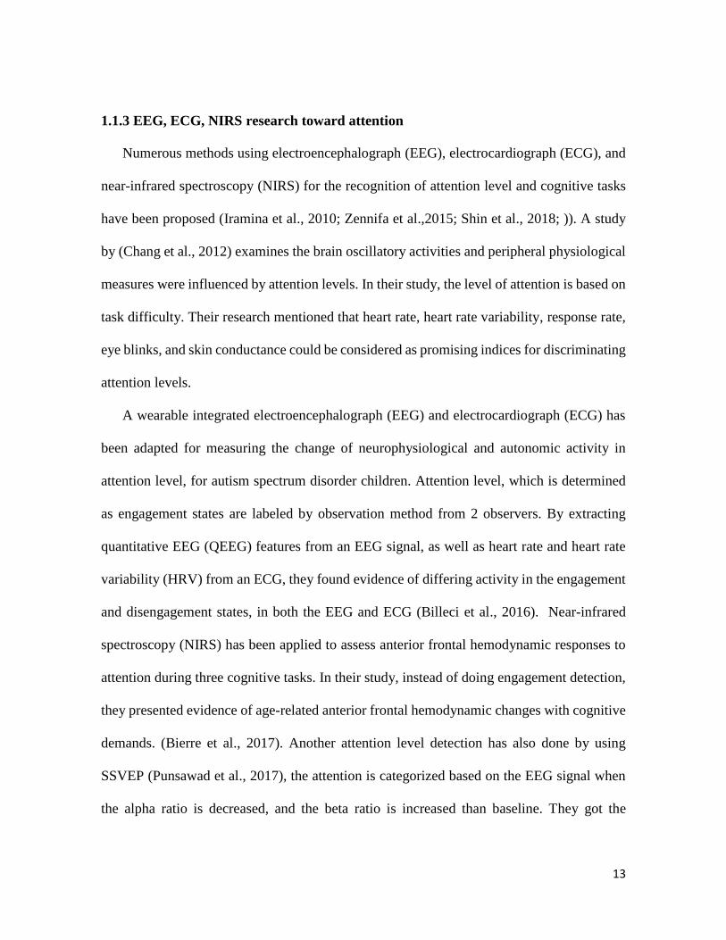
1.1.3 EEG, ECG, NIRS research toward attention

Numerous methods using electroencephalograph (EEG), electrocardiograph (ECG), and

near-infrared spectroscopy (NIRS) for the recognition of attention level and cognitive tasks

have been proposed (Iramina et al., 2010; Zennifa et al.,2015; Shin et al., 2018; )). A study

by (Chang et al., 2012) examines the brain oscillatory activities and peripheral physiological

measures were influenced by attention levels. In their study, the level of attention is based on

task difficulty. Their research mentioned that heart rate, heart rate variability, response rate,

eye blinks, and skin conductance could be considered as promising indices for discriminating

attention levels.

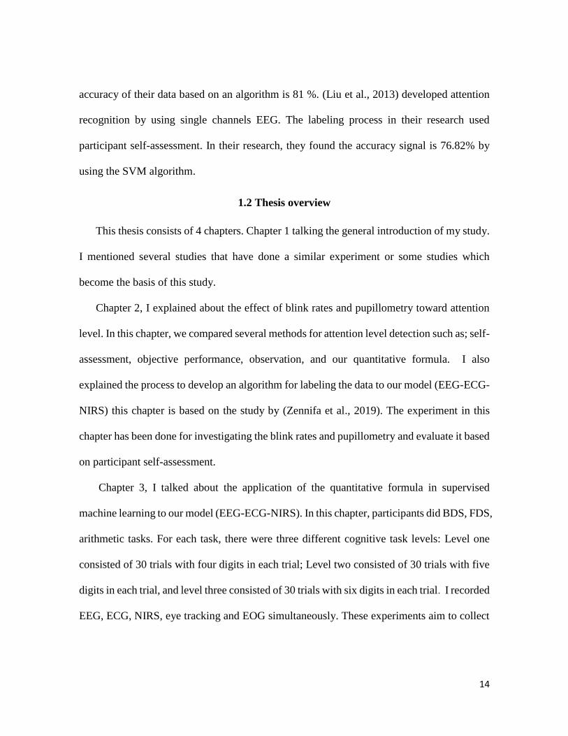
A wearable integrated electroencephalograph (EEG) and electrocardiograph (ECG) has

been adapted for measuring the change of neurophysiological and autonomic activity in

attention level, for autism spectrum disorder children. Attention level, which is determined

as engagement states are labeled by observation method from 2 observers. By extracting

quantitative EEG (QEEG) features from an EEG signal, as well as heart rate and heart rate

variability (HRV) from an ECG, they found evidence of differing activity in the engagement

and disengagement states, in both the EEG and ECG (Billeci et al., 2016). Near-infrared

spectroscopy (NIRS) has been applied to assess anterior frontal hemodynamic responses to

attention during three cognitive tasks. In their study, instead of doing engagement detection,

they presented evidence of age-related anterior frontal hemodynamic changes with cognitive

demands. (Bierre et al., 2017). Another attention level detection has also done by using

SSVEP (Punsawad et al., 2017), the attention is categorized based on the EEG signal when

the alpha ratio is decreased, and the beta ratio is increased than baseline. They got the

14

accuracy of their data based on an algorithm is 81 %. (Liu et al., 2013) developed attention

recognition by using single channels EEG. The labeling process in their research used

participant self-assessment. In their research, they found the accuracy signal is 76.82% by

using the SVM algorithm.

1.2 Thesis overview

This thesis consists of 4 chapters. Chapter 1 talking the general introduction of my study.

I mentioned several studies that have done a similar experiment or some studies which

become the basis of this study.

Chapter 2, I explained about the effect of blink rates and pupillometry toward attention

level. In this chapter, we compared several methods for attention level detection such as; self-

assessment, objective performance, observation, and our quantitative formula. I also

explained the process to develop an algorithm for labeling the data to our model (EEG-ECG-

NIRS) this chapter is based on the study by (Zennifa et al., 2019). The experiment in this

chapter has been done for investigating the blink rates and pupillometry and evaluate it based

on participant self-assessment.

Chapter 3, I talked about the application of the quantitative formula in supervised

machine learning to our model (EEG-ECG-NIRS). In this chapter, participants did BDS, FDS,

arithmetic tasks. For each task, there were three different cognitive task levels: Level one

consisted of 30 trials with four digits in each trial; Level two consisted of 30 trials with five

digits in each trial, and level three consisted of 30 trials with six digits in each trial. I recorded

EEG, ECG, NIRS, eye tracking and EOG simultaneously. These experiments aim to collect

15

the data and applied the quantitative formula in data labeling for further application in

supervised machine learning.

Chapter 4, The last chapter in this study, we talked about the general discussion of this

thesis. This chapter aims to mention all founding that we have and the limitation of my study.

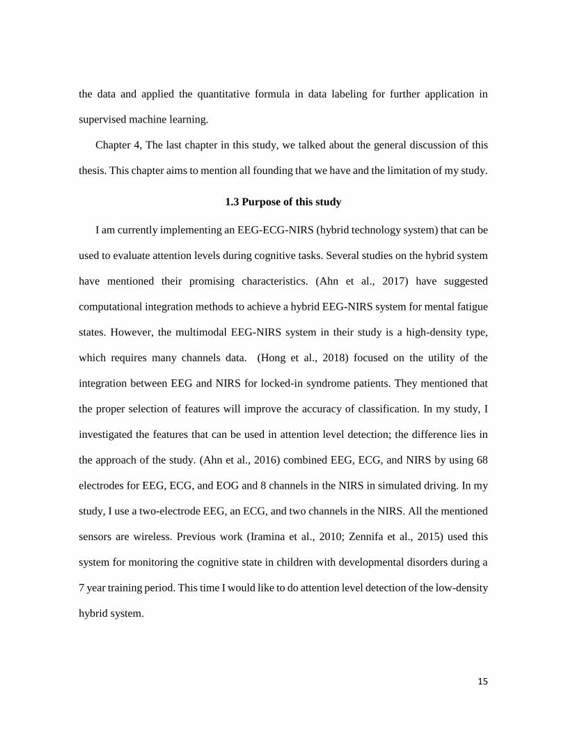
1.3 Purpose of this study

I am currently implementing an EEG-ECG-NIRS (hybrid technology system) that can be

used to evaluate attention levels during cognitive tasks. Several studies on the hybrid system

have mentioned their promising characteristics. (Ahn et al., 2017) have suggested

computational integration methods to achieve a hybrid EEG-NIRS system for mental fatigue

states. However, the multimodal EEG-NIRS system in their study is a high-density type,

which requires many channels data. (Hong et al., 2018) focused on the utility of the

integration between EEG and NIRS for locked-in syndrome patients. They mentioned that

the proper selection of features will improve the accuracy of classification. In my study, I

investigated the features that can be used in attention level detection; the difference lies in

the approach of the study. (Ahn et al., 2016) combined EEG, ECG, and NIRS by using 68

electrodes for EEG, ECG, and EOG and 8 channels in the NIRS in simulated driving. In my

study, I use a two-electrode EEG, an ECG, and two channels in the NIRS. All the mentioned

sensors are wireless. Previous work (Iramina et al., 2010; Zennifa et al., 2015) used this

system for monitoring the cognitive state in children with developmental disorders during a

7 year training period. This time I would like to do attention level detection of the low-density

hybrid system.

16

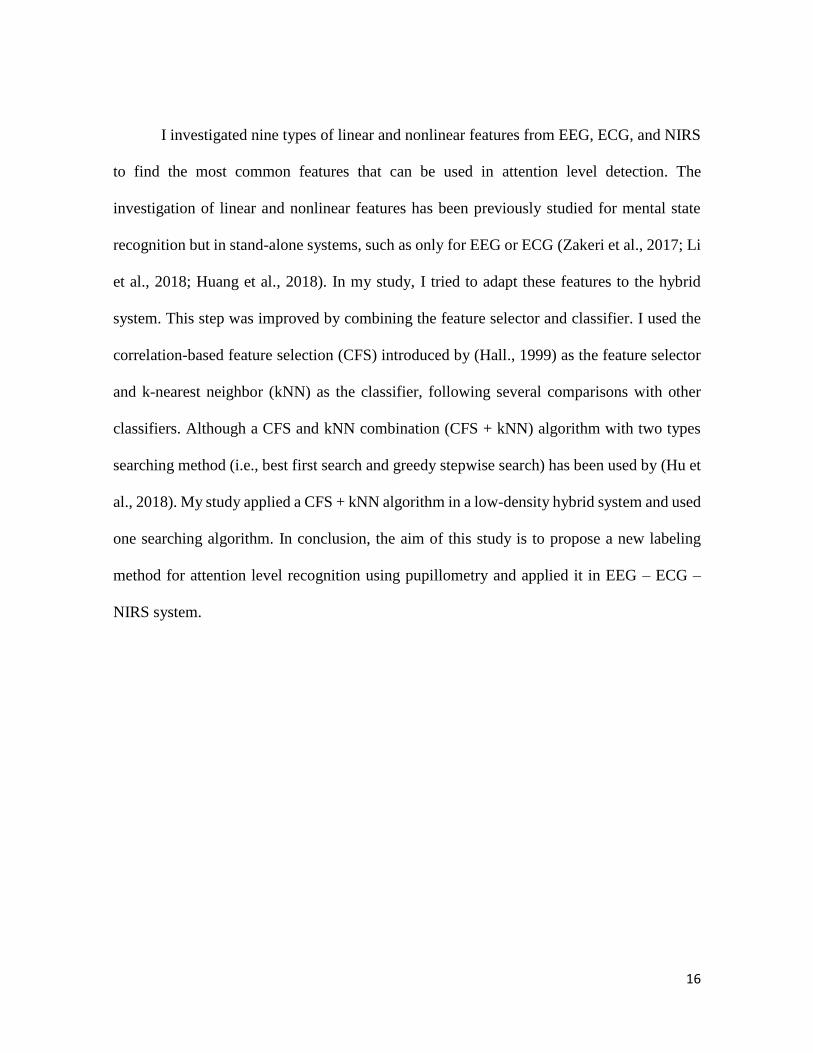
I investigated nine types of linear and nonlinear features from EEG, ECG, and NIRS

to find the most common features that can be used in attention level detection. The

investigation of linear and nonlinear features has been previously studied for mental state

recognition but in stand-alone systems, such as only for EEG or ECG (Zakeri et al., 2017; Li

et al., 2018; Huang et al., 2018). In my study, I tried to adapt these features to the hybrid

system. This step was improved by combining the feature selector and classifier. I used the

correlation-based feature selection (CFS) introduced by (Hall., 1999) as the feature selector

and k-nearest neighbor (kNN) as the classifier, following several comparisons with other

classifiers. Although a CFS and kNN combination (CFS + kNN) algorithm with two types

searching method (i.e., best first search and greedy stepwise search) has been used by (Hu et

al., 2018). My study applied a CFS + kNN algorithm in a low-density hybrid system and used

one searching algorithm. In conclusion, the aim of this study is to propose a new labeling

method for attention level recognition using pupillometry and applied it in EEG – ECG –

NIRS system.

17

Chapter 2. New Labelling method for attention level detection

2.1 Abstract

Attention is described as a state in which an individual involved in an activity can ignore

other influences. The attention level is important to obtain good performance, especially

under study conditions. Numerous methods for attention level detection such as observation,

self-assessment, objective performance and physiology signal has been applied. In this

chapter, I tried to develop a labelling method based on physiological data (blink rates and

pupillometry).

In this chapter, I compared the self-assessment method with other attention level

detection methods (observation and objective performance). The aim of this comparison is

to know the differences evaluation between self –assessments and other methods. From this

comparison, I got the difference of self-assessment toward other method is lower than 21%.

After that, I investigated the effect of attention level based on self-assessment to blink rates,

and pupillometry. I found that pupillometry in low attention is smaller than high attention

especially in the last 4 second encoding time (P<0.05). On the other hand, I did not get a

significant difference in blink rates. After that, I calculated the distribution fit of pupillometry

reaction in the attention level of all participants and plot the critical point of pupillometry

data in 10 seconds and 4 seconds. After doing several experimental procedures, I chose

parameter setting by comparing with self-assessment with a percentage of error of less than

15% and a different error 35 % as future labeling method. Parameter setting which has been

selected is when z-score within a specific range (-0.965 ≤ pupil ≤ 1.014) as high attention,

other that range, will be classified as low attention.

18

2.2. Materials and Methods

2.2.1 Participants

There were 18 participants in my experiment. All participants were Kyushu University

students, with ages ranging from 21 to 29 (23.5 ± 2.18). All participants had a normal visual

function and were free of disability; 15 were right-handed, 1 participant was ambidextrous,

and 2 participant was left-handed. Participants were instructed not to consume any caffeine

2 h before the experiment because it could affect the HRV (Martínez-Sellés et al., 2013;

Oliveira et al., 2017). The study was conducted by following the ethical principles of Kyushu

University and the Declaration of Helsinki. Written informed consent was obtained from

each participant before the experiment as showed on Appendix 1.

2.2.2 Experiment condition

The experiment took place in a dimly lit room. I also recorded the behavior activities

using a webcam camera (Logicool C270, Logitech, Switzerland), which was located around

57 cm in front of the participant’s face.

Three types of attention task were used: backward digit span (BDS) (Jensen et al., 1975;

Cullum., 1998; Berka et al 2007, Zennifa et al., 2018; Zennifa et al., 2019; Rosenthal et al.,

2006), forward digit span (FDS) (Jensen et al., 1975; Cullum., 1998; Berka et al 2007,

Zennifa et al., 2018; Zennifa et al., 2019; Rosenthal et al., 2006) and arithmetic (Zennifa et

al., 2018). These tasks consist of three-level. Level one consisted of a series of 20 sets of four

digits, level two: 20 sets of five digits and level three: 20 sets of six digits. Most of the

questions in this experiment were relatively simple and did not require any prerequisite

knowledge or specific skills. However, a good level of attention and alertness was required

19

to avoid making easy mistakes because the response time was limited to 15 s. Each trial

started with the presentation of a central, white fixation dot on a dark background until the

participant’s eyes could be accepted by the eye tracker. Next, cognitive questions (i.e.,

encoding session) would appear for 10 s and the participant was instructed to respond within

15 s. Digits will appear every 2.5 seconds in 4 digit level, 2 seconds in 5 digit level and 1.67

seconds in 6 digit level. After that, participants should report their attention level in two

conditions, high or low. All cognitive tasks were counterbalanced. The measurement was

recorded after the practice session finished. The task can be seen in Figure1.

Figure 1. Task design example

2.2.3. Software and Apparatus

In this chapter, the 17-inch CRT monitor (1024 × 768) has been used for presenting the

stimuli. Testing took place in a dimly lit room. Stimuli presentation was done by using

OpenSesame (Mathôt et al., 2012), using the legacy back end for the display control and the

PyGaze toolbox (Dalmaijer., 2014) for integrating to the eye tracker.

20

2.2.3.1 Eye Tracking

Before the start of each task, participants were positioned in front of an eye tracker (The

EyeTribe tracker version 1, Copenhagen, Denmark). The distance of the participants' eyes

from The EyeTribe was estimated to be ~57 cm. The participants were asked to fix their

heads on a chin rest. In this study, we calibrated and validated the eye-tracking system to

each participant using a nine-point dot matrix. After validation, the eye tracker that had been

embedded with the OpenSesame software labeled each calibration point with the error in the

degree of the visual angle between the calibrated and validated measures. If the calibration

points do not exceed 1° (degree) and the greatest single point error does not exceed 1°, the

process would continue. Before each trial, a one-point eye tracker recalibration was

performed.

2.2.3.2 Electrooculogram

In this study, EOG (Polymate Mini AP 108, Miyuki Giken Co., Ltd., Kasugai-city, Japan)

signals were sent by Bluetooth to a computer. The frequency of sampling was 500 Hz. We

put two electrodes for a vertical EOG. This location was chosen to detect blink(Waters et

al.,2005 ; Huang et al, .2018). Figure 2 shows the electrode placements.

21

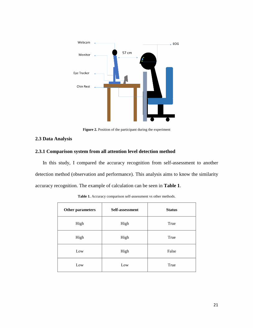
Figure 2. Position of the participant during the experiment

2.3 Data Analysis

2.3.1 Comparison system from all attention level detection method

In this study, I compared the accuracy recognition from self-assessment to another

detection method (observation and performance). This analysis aims to know the similarity

accuracy recognition. The example of calculation can be seen in Table 1.

Table 1. Accuracy comparison self-assessment vs other methods.

Other parameters Self-assessment Status

High High True

High High True

Low High False

Low Low True

22

Based on data from Table 1, I calculated difference rate error and error rate detection based

on formula (1) and formula (2).

Difference error is difference status between self-assessment and another method in each trial.

Error detection is the different status between self-assessment and another method in all trials.

Total trials means the number of all trials that has been done by each participant.

2.3.2 Blink rates and pupillometry analysis

After getting results from participant self-assessment and another recognition method, I

started to analyze the blink rates and pupillometry. I would like to check the effect of attention

based on self-assessment toward blink rates and pupillomery. Below is the explanation how

do I analyze blink rates and pupillometry.

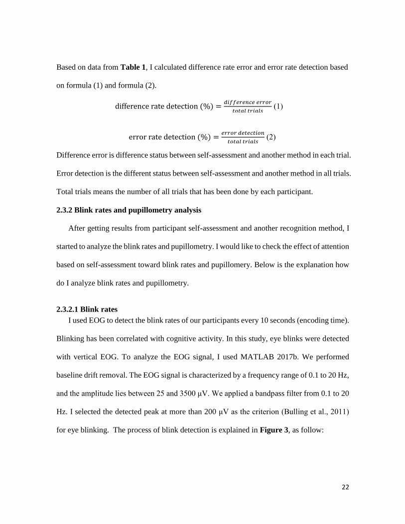
2.3.2.1 Blink rates

I used EOG to detect the blink rates of our participants every 10 seconds (encoding time).

Blinking has been correlated with cognitive activity. In this study, eye blinks were detected

with vertical EOG. To analyze the EOG signal, I used MATLAB 2017b. We performed

baseline drift removal. The EOG signal is characterized by a frequency range of 0.1 to 20 Hz,

and the amplitude lies between 25 and 3500 μV. We applied a bandpass filter from 0.1 to 20

Hz. I selected the detected peak at more than 200 μV as the criterion (Bulling et al., 2011)

for eye blinking. The process of blink detection is explained in Figure 3, as follow:

difference rate detection (%) =𝑑𝑖𝑓𝑓𝑒𝑟𝑒𝑛𝑐𝑒 𝑒𝑟𝑟𝑜𝑟

𝑡𝑜𝑡𝑎𝑙 𝑡𝑟𝑖𝑎𝑙𝑠 (1)

error rate detection (%) =𝑒𝑟𝑟𝑜𝑟 𝑑𝑒𝑡𝑒𝑐𝑡𝑖𝑜𝑛

𝑡𝑜𝑡𝑎𝑙 𝑡𝑟𝑖𝑎𝑙𝑠 (2)

23

Figure 3. Blink detection

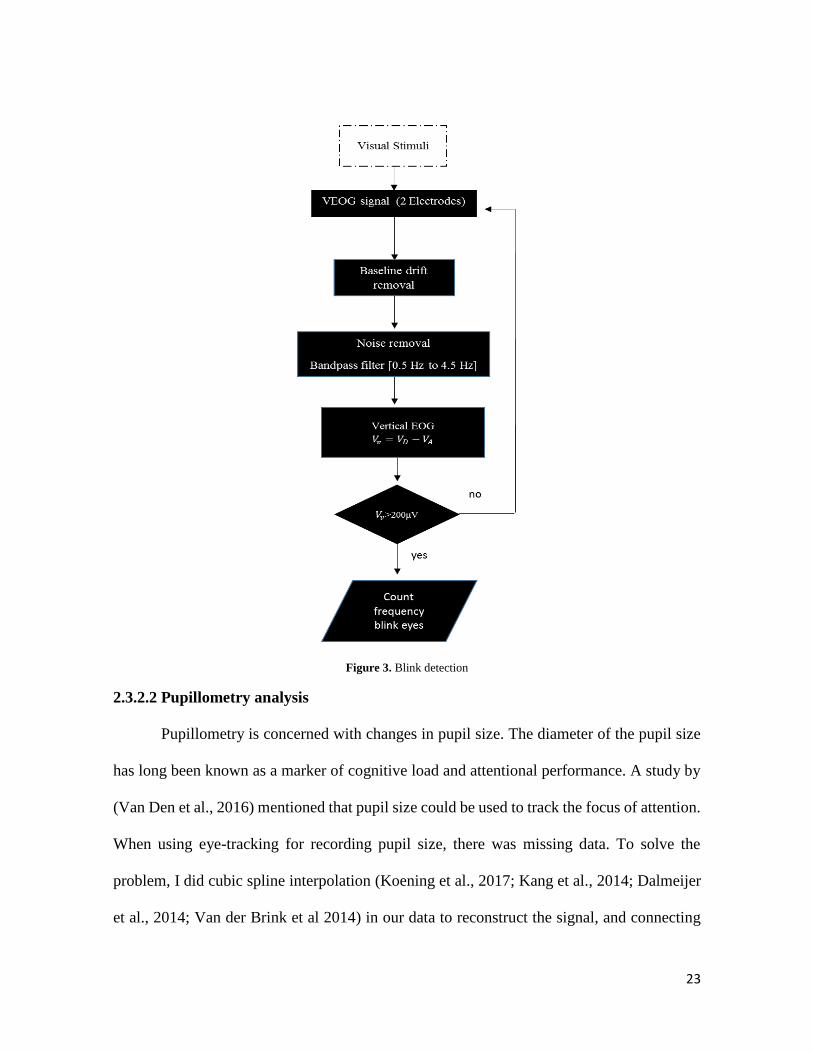
2.3.2.2 Pupillometry analysis

Pupillometry is concerned with changes in pupil size. The diameter of the pupil size

has long been known as a marker of cognitive load and attentional performance. A study by

(Van Den et al., 2016) mentioned that pupil size could be used to track the focus of attention.

When using eye-tracking for recording pupil size, there was missing data. To solve the

problem, I did cubic spline interpolation (Koening et al., 2017; Kang et al., 2014; Dalmeijer

et al., 2014; Van der Brink et al 2014) in our data to reconstruct the signal, and connecting

24

the missing data. Figure 4 is shown signal differences before interpolation and after

interpolation.

Figure 4. Signal reconstruction

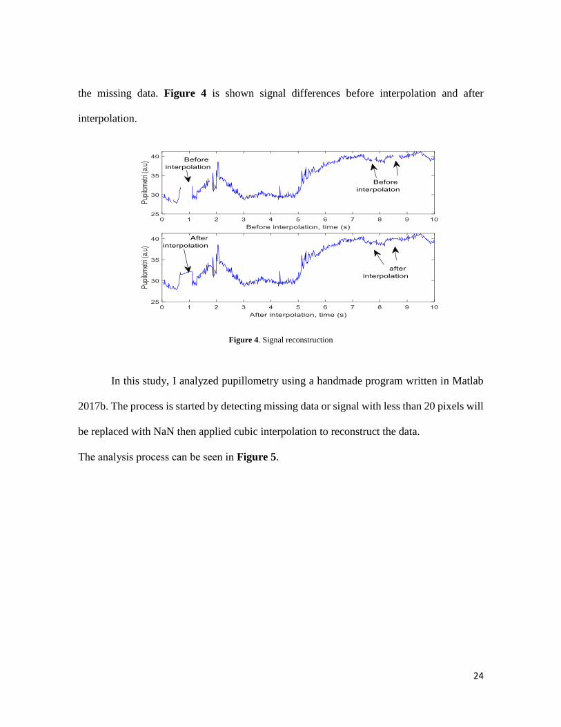
In this study, I analyzed pupillometry using a handmade program written in Matlab

2017b. The process is started by detecting missing data or signal with less than 20 pixels will

be replaced with NaN then applied cubic interpolation to reconstruct the data.

The analysis process can be seen in Figure 5.

25

Figure 5. Pupillometry analysis

After getting the value of pupil size, considering difference of each individual data, I

converted the value of raw pupillometry to Z-score, as showed in Equation (3):

Zpupil=𝑥𝑠𝑎𝑚𝑝𝑙𝑒−𝜇𝑝𝑜𝑝𝑢𝑙𝑎𝑡𝑖𝑜𝑛

𝑆𝑑𝑝𝑜𝑝𝑢𝑙𝑎𝑡𝑖𝑜𝑛 (3)

Where 𝑥𝑠𝑎𝑚𝑝𝑙𝑒 is participant pupillometry in each trial.

𝜇𝑝𝑜𝑝𝑢𝑙𝑎𝑡𝑖𝑜𝑛 is average participant pupillometry in all trials.

𝑆𝑑𝑝𝑜𝑝𝑢𝑙𝑎𝑡𝑖𝑜𝑛is standard deviation of pupillometry in all trials

2.3.2.3 Data balancing

Because my data based on states (High attention and Low attention) are imbalances, I need

to anticipate this event by re-sampling my data (Chicco et al, 2017). In my study, I applied oversample

technique as solution for my imbalance data. Oversampling means to increase the number of minority

26

class members in dataset. By using over-sampling there is no information from the original training

set is lost since all members from the minority and majority classes are kept. (Rahman et al., 2013;

Chawla et al., 2018). Balancing is applied when plotted histogram all participants data into one dataset.

2.4 Results

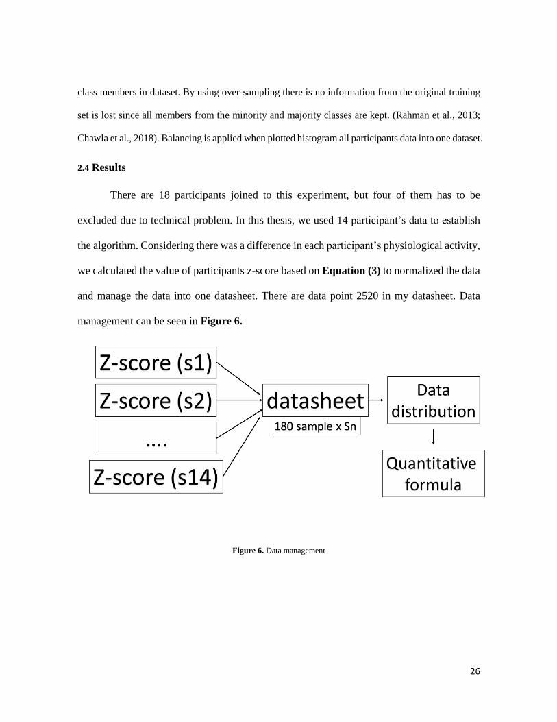
There are 18 participants joined to this experiment, but four of them has to be

excluded due to technical problem. In this thesis, we used 14 participant’s data to establish

the algorithm. Considering there was a difference in each participant’s physiological activity,

we calculated the value of participants z-score based on Equation (3) to normalized the data

and manage the data into one datasheet. There are data point 2520 in my datasheet. Data

management can be seen in Figure 6.

Figure 6. Data management

27

2.4.1 Self-assessment reliability for the basis on quantitative formula

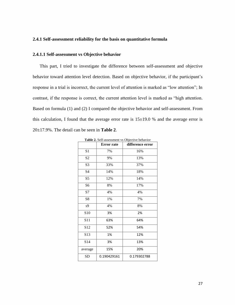
2.4.1.1 Self-assessment vs Objective behavior

This part, I tried to investigate the difference between self-assessment and objective

behavior toward attention level detection. Based on objective behavior, if the participant’s

response in a trial is incorrect, the current level of attention is marked as “low attention”; In

contrast, if the response is correct, the current attention level is marked as “high attention.

Based on formula (1) and (2) I compared the objective behavior and self-assessment. From

this calculation, I found that the average error rate is 15±19.0 % and the average error is

20±17.9%. The detail can be seen in Table 2.

Table 2. Self-assessment vs Objective behavior

Error rate difference error

S1 7% 16%

S2 9% 13%

S3 33% 37%

S4 14% 18%

S5 12% 14%

S6 8% 17%

S7 4% 4%

S8 1% 7%

s9 4% 8%

S10 3% 2%

S11 63% 64%

S12 52% 54%

S13 1% 12%

S14 3% 13%

average 15% 20%

SD 0.190429161 0.179302788

28

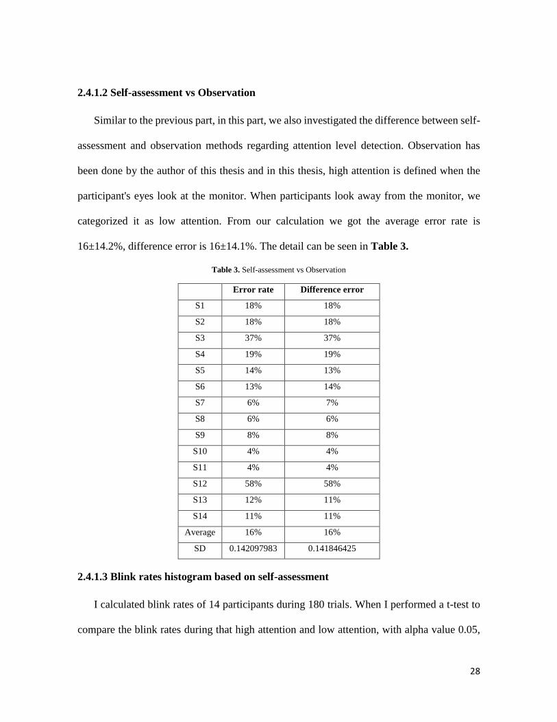
2.4.1.2 Self-assessment vs Observation

Similar to the previous part, in this part, we also investigated the difference between self-

assessment and observation methods regarding attention level detection. Observation has

been done by the author of this thesis and in this thesis, high attention is defined when the

participant's eyes look at the monitor. When participants look away from the monitor, we

categorized it as low attention. From our calculation we got the average error rate is

16±14.2%, difference error is 16±14.1%. The detail can be seen in Table 3.

Table 3. Self-assessment vs Observation

Error rate Difference error

S1 18% 18%

S2 18% 18%

S3 37% 37%

S4 19% 19%

S5 14% 13%

S6 13% 14%

S7 6% 7%

S8 6% 6%

S9 8% 8%

S10 4% 4%

S11 4% 4%

S12 58% 58%

S13 12% 11%

S14 11% 11%

Average 16% 16%

SD 0.142097983 0.141846425

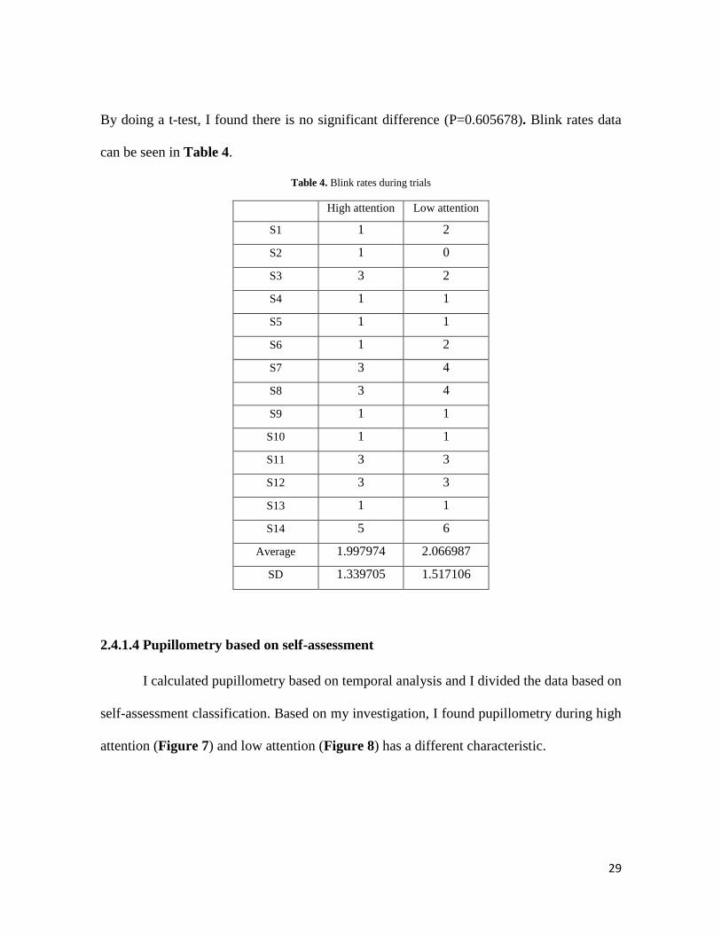
2.4.1.3 Blink rates histogram based on self-assessment

I calculated blink rates of 14 participants during 180 trials. When I performed a t-test to

compare the blink rates during that high attention and low attention, with alpha value 0.05,

29

By doing a t-test, I found there is no significant difference (P=0.605678). Blink rates data

can be seen in Table 4.

Table 4. Blink rates during trials

High attention Low attention

S1 1 2

S2 1 0

S3 3 2

S4 1 1

S5 1 1

S6 1 2

S7 3 4

S8 3 4

S9 1 1

S10 1 1

S11 3 3

S12 3 3

S13 1 1

S14 5 6

Average 1.997974 2.066987

SD 1.339705 1.517106

2.4.1.4 Pupillometry based on self-assessment

I calculated pupillometry based on temporal analysis and I divided the data based on

self-assessment classification. Based on my investigation, I found pupillometry during high

attention (Figure 7) and low attention (Figure 8) has a different characteristic.

30

Figure 7. High attention in each trial

Figure 8. Low attention in each trial

After calculating the data from each participant in each trial, I found that average

pupil size in pupillometry has a tendency to be decreasing in low attention and tends to be

stable in high attention in the temporal analysis. Following that, I also found that

pupillometry in high attention has a bigger size rather than in low attention.

Figure 9. Temporal analysis pupillometry n= 14

31

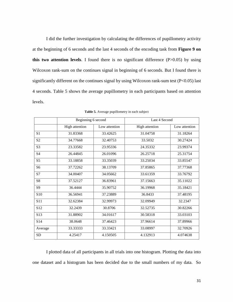
I did the further investigation by calculating the differences of pupillometry activity

at the beginning of 6 seconds and the last 4 seconds of the encoding task from Figure 9 on

this two attention levels. I found there is no significant difference (P>0.05) by using

Wilcoxon rank-sum on the continues signal in beginning of 6 seconds. But I found there is

significantly different on the continues signal by using Wilcoxon rank-sum test (P<0.05) last

4 seconds. Table 5 shows the average pupillometry in each participants based on attention

levels.

Table 5. Average pupillometry in each subject

Beginning 6 second Last 4 Second

High attention Low attention High attention Low attention

S1 31.83368 33.42625 31.04758 31.18264

S2 34.77668 32.40753 33.5032 30.27424

S3 23.33582 23.95336 24.35332 23.99374

S4 26.44845 26.01096 26.25718 25.31754

S5 33.18858 33.35039 33.25034 33.85547

S6 37.72262 38.13709 37.85865 37.77368

S7 34.00407 34.05662 33.61359 33.76792

S8 37.52127 36.83961 37.15663 35.11022

S9 36.4444 35.90752 36.19968 35.18421

S10 36.56941 37.23889 36.8433 37.48195

S11 32.62384 32.99973 32.09949 32.2347

S12 32.2439 30.8706 32.52735 30.82266

S13 31.88902 34.01617 30.58318 33.03103

S14 38.0648 37.46423 37.96614 37.89966

Average 33.33333 33.33421 33.08997 32.70926

SD 4.25417 4.150505 4.132913 4.074638

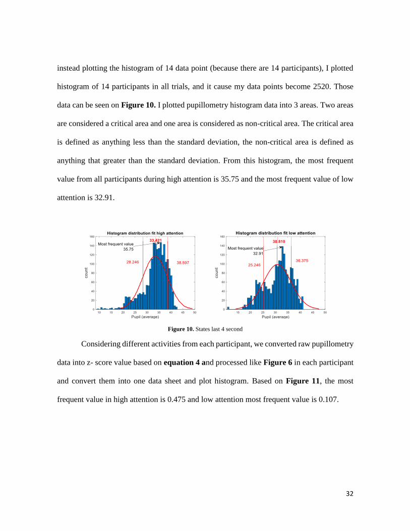
I plotted data of all participants in all trials into one histogram. Plotting the data into

one dataset and a histogram has been decided due to the small numbers of my data. So

32

instead plotting the histogram of 14 data point (because there are 14 participants), I plotted

histogram of 14 participants in all trials, and it cause my data points become 2520. Those

data can be seen on Figure 10. I plotted pupillometry histogram data into 3 areas. Two areas

are considered a critical area and one area is considered as non-critical area. The critical area

is defined as anything less than the standard deviation, the non-critical area is defined as

anything that greater than the standard deviation. From this histogram, the most frequent

value from all participants during high attention is 35.75 and the most frequent value of low

attention is 32.91.

Figure 10. States last 4 second

Considering different activities from each participant, we converted raw pupillometry

data into z- score value based on equation 4 and processed like Figure 6 in each participant

and convert them into one data sheet and plot histogram. Based on Figure 11, the most

frequent value in high attention is 0.475 and low attention most frequent value is 0.107.

33

Figure 11. Z-score last 4 second

2.4.2 Parameter settings for attention level

2.4.2.1 Extracting Pupillometry in 10 s to parameter settings

In this session, I tried to extracted data from histogram distribution during high

attention and low attention to several thresholds for labeling. Average of ten-second data is

used and converted to z-score, I divided data into 3 criteria (2 critical areas and 1 noncritical

area). For further labeling is extracted from data in the non-critical area. The process to

extract parameter setting for labeling is as follow:

34

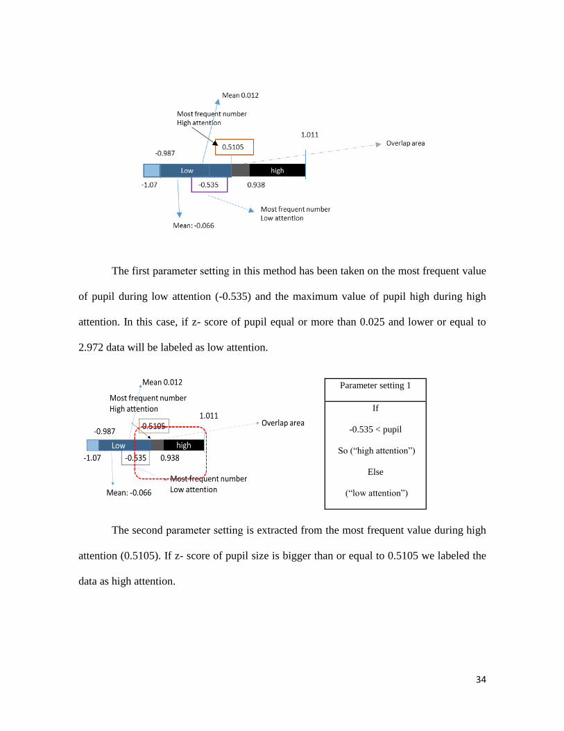
The first parameter setting in this method has been taken on the most frequent value

of pupil during low attention (-0.535) and the maximum value of pupil high during high

attention. In this case, if z- score of pupil equal or more than 0.025 and lower or equal to

2.972 data will be labeled as low attention.

The second parameter setting is extracted from the most frequent value during high

attention (0.5105). If z- score of pupil size is bigger than or equal to 0.5105 we labeled the

data as high attention.

Parameter setting 1

If

-0.535 < pupil

So (“high attention”)

Else

(“low attention”)

35

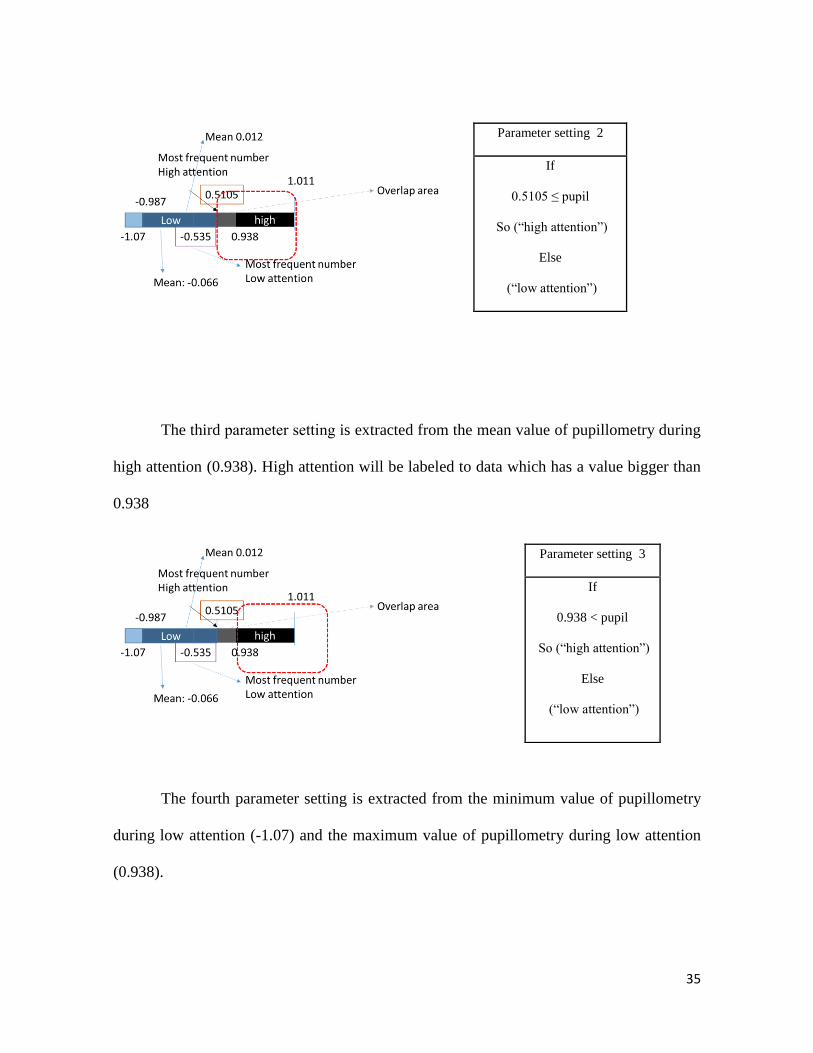
The third parameter setting is extracted from the mean value of pupillometry during

high attention (0.938). High attention will be labeled to data which has a value bigger than

0.938

The fourth parameter setting is extracted from the minimum value of pupillometry

during low attention (-1.07) and the maximum value of pupillometry during low attention

(0.938).

Parameter setting 2

If

0.5105 ≤ pupil


Else


Parameter setting 3

If

0.938 < pupil


Else


36

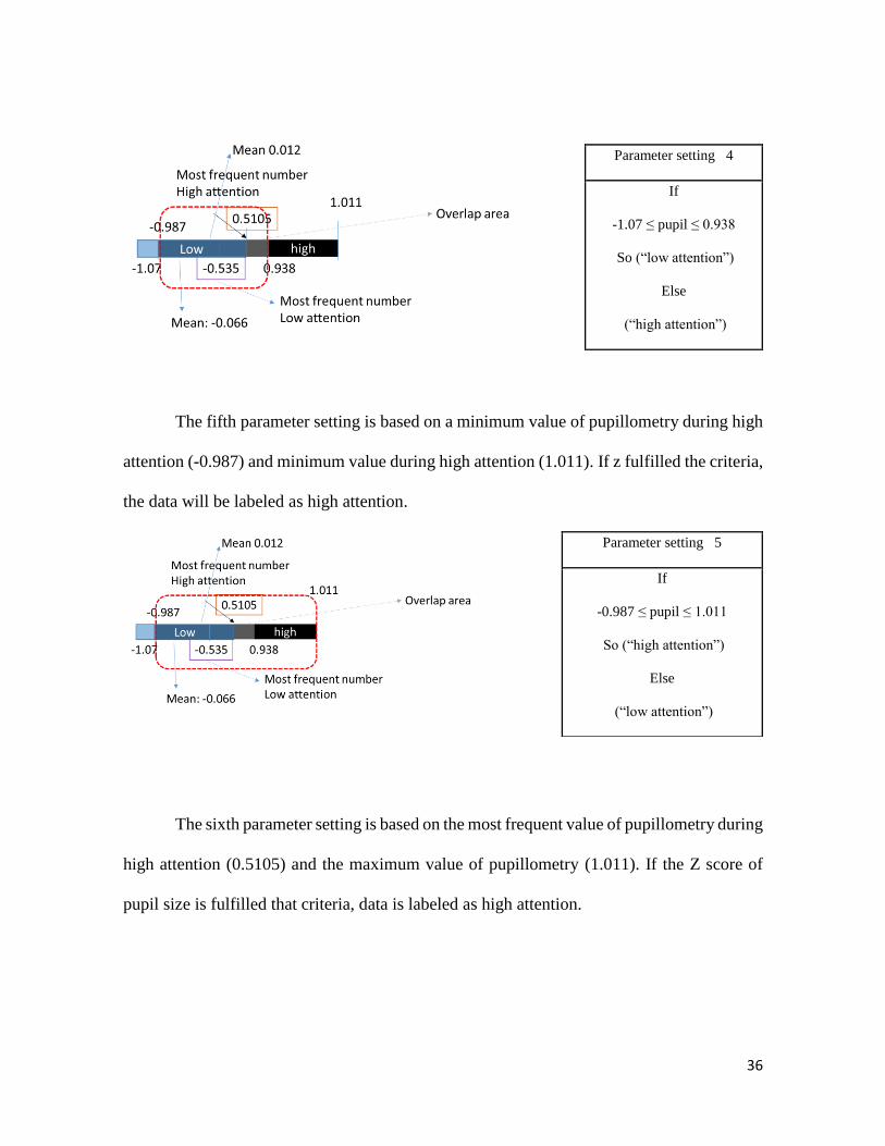
The fifth parameter setting is based on a minimum value of pupillometry during high

attention (-0.987) and minimum value during high attention (1.011). If z fulfilled the criteria,

the data will be labeled as high attention.

The sixth parameter setting is based on the most frequent value of pupillometry during

high attention (0.5105) and the maximum value of pupillometry (1.011). If the Z score of

pupil size is fulfilled that criteria, data is labeled as high attention.

Parameter setting 4

If

-1.07 ≤ pupil ≤ 0.938

So (“low attention”)

Else

(“high attention”)

Parameter setting 5

If

-0.987 ≤ pupil ≤ 1.011


Else


37

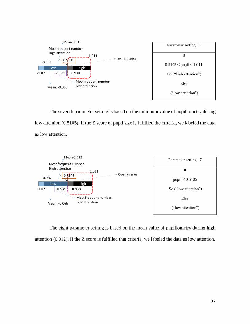
The seventh parameter setting is based on the minimum value of pupillometry during

low attention (0.5105). If the Z score of pupil size is fulfilled the criteria, we labeled the data

as low attention.

The eight parameter setting is based on the mean value of pupillometry during high

attention (0.012). If the Z score is fulfilled that criteria, we labeled the data as low attention.

Parameter setting 6

If

0.5105 ≤ pupil ≤ 1.011


Else


Parameter setting 7

If

pupil < 0.5105


Else


38

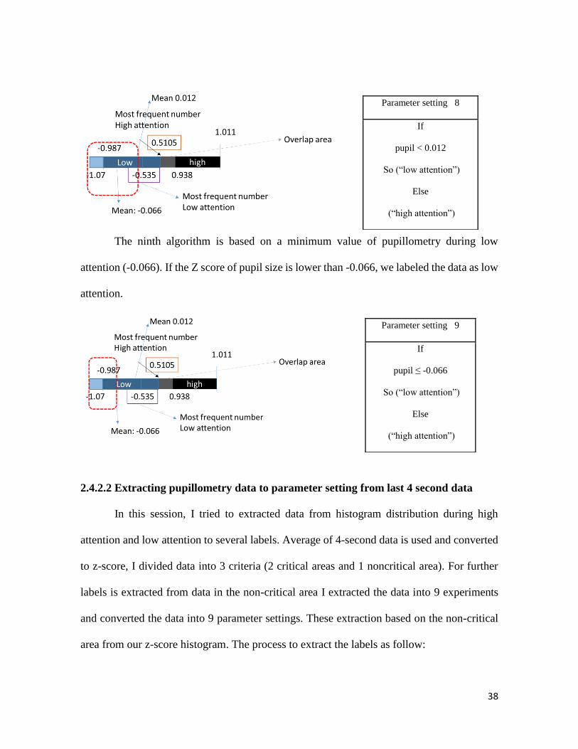
The ninth algorithm is based on a minimum value of pupillometry during low

attention (-0.066). If the Z score of pupil size is lower than -0.066, we labeled the data as low

attention.

2.4.2.2 Extracting pupillometry data to parameter setting from last 4 second data

In this session, I tried to extracted data from histogram distribution during high

attention and low attention to several labels. Average of 4-second data is used and converted

to z-score, I divided data into 3 criteria (2 critical areas and 1 noncritical area). For further

labels is extracted from data in the non-critical area I extracted the data into 9 experiments

and converted the data into 9 parameter settings. These extraction based on the non-critical

area from our z-score histogram. The process to extract the labels as follow:

Parameter setting 8

If

pupil < 0.012


Else


Parameter setting 9

If

pupil ≤ -0.066


Else


39

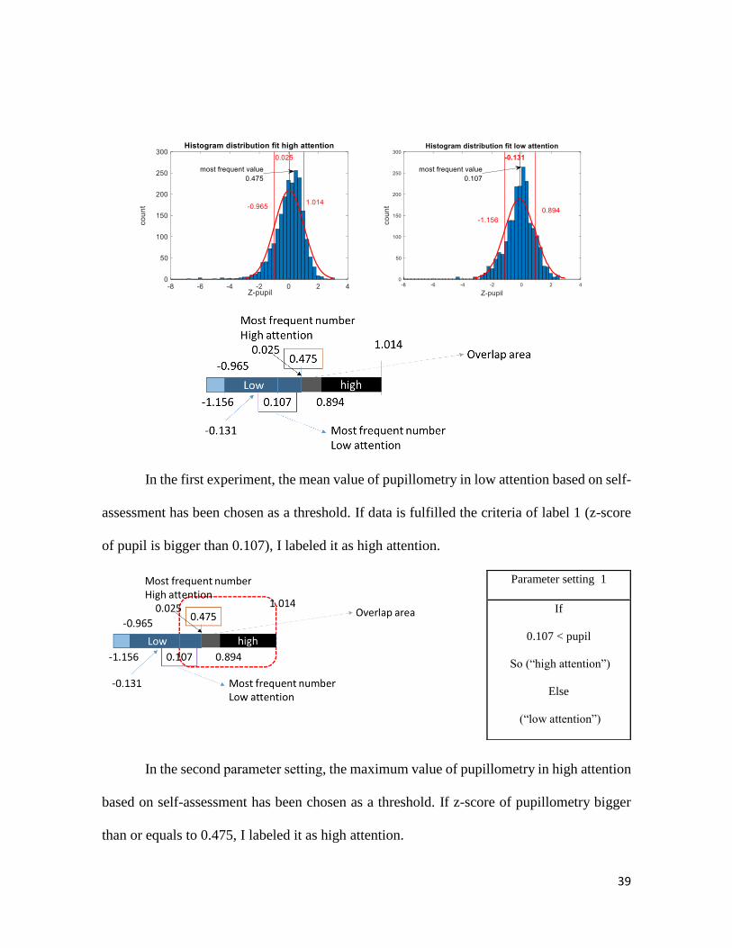
In the first experiment, the mean value of pupillometry in low attention based on self-

assessment has been chosen as a threshold. If data is fulfilled the criteria of label 1 (z-score

of pupil is bigger than 0.107), I labeled it as high attention.

In the second parameter setting, the maximum value of pupillometry in high attention

based on self-assessment has been chosen as a threshold. If z-score of pupillometry bigger

than or equals to 0.475, I labeled it as high attention.

Parameter setting 1

If

0.107 < pupil


Else


40

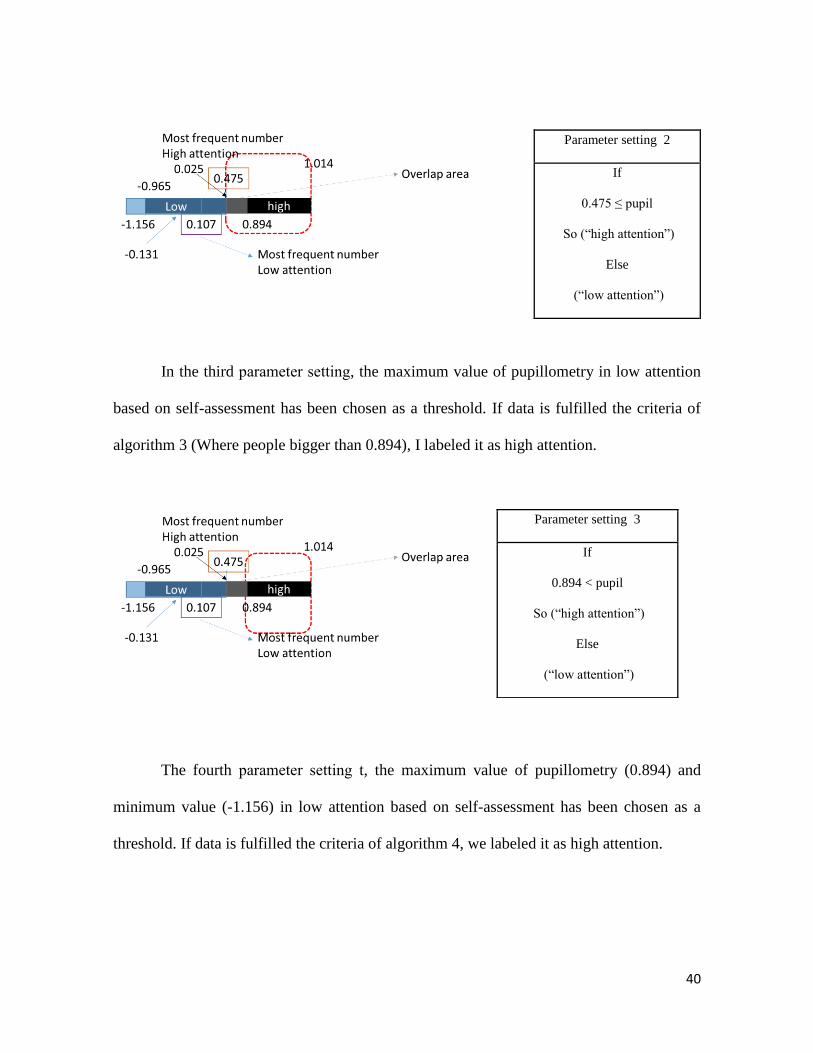
In the third parameter setting, the maximum value of pupillometry in low attention

based on self-assessment has been chosen as a threshold. If data is fulfilled the criteria of

algorithm 3 (Where people bigger than 0.894), I labeled it as high attention.

The fourth parameter setting t, the maximum value of pupillometry (0.894) and

minimum value (-1.156) in low attention based on self-assessment has been chosen as a

threshold. If data is fulfilled the criteria of algorithm 4, we labeled it as high attention.

Parameter setting 2

If

0.475 ≤ pupil


Else


Parameter setting 3

If

0.894 < pupil


Else


41

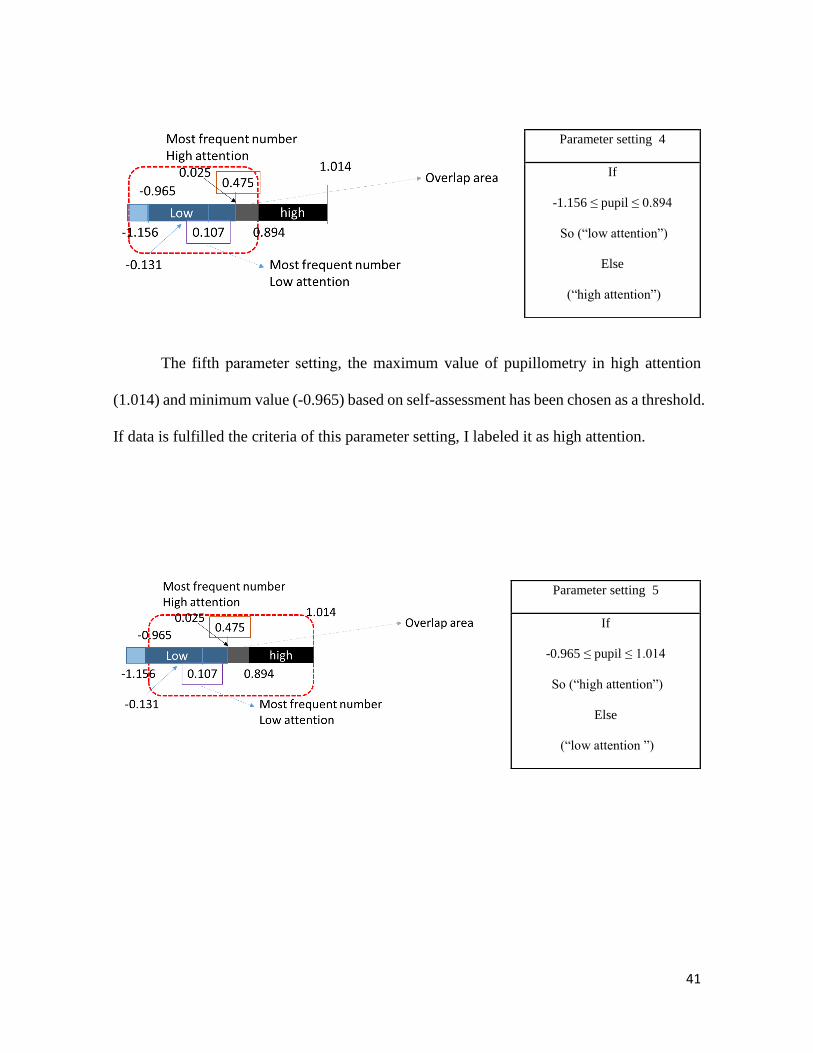
The fifth parameter setting, the maximum value of pupillometry in high attention

(1.014) and minimum value (-0.965) based on self-assessment has been chosen as a threshold.

If data is fulfilled the criteria of this parameter setting, I labeled it as high attention.

Parameter setting 4

If

-1.156 ≤ pupil ≤ 0.894


Else


Parameter setting 5

If

-0.965 ≤ pupil ≤ 1.014


Else

(“low attention ”)

42

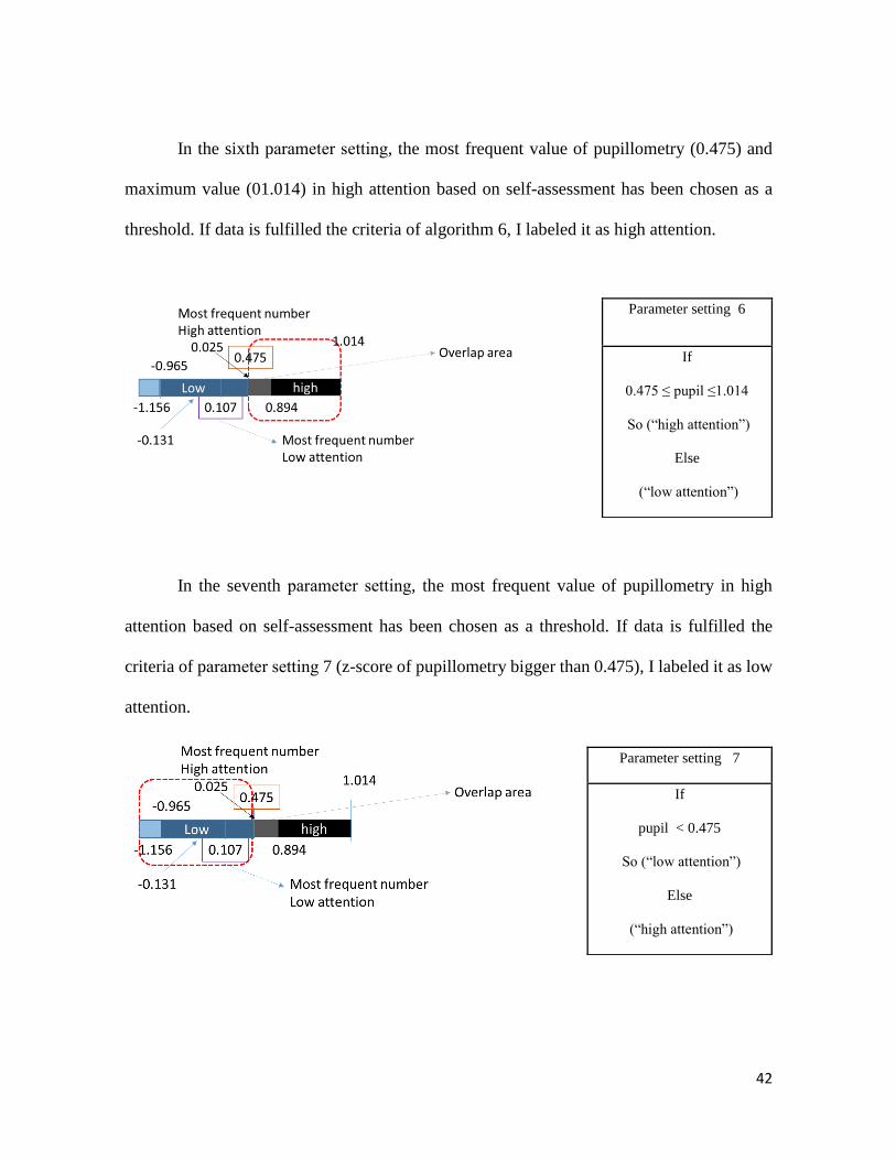
In the sixth parameter setting, the most frequent value of pupillometry (0.475) and

maximum value (01.014) in high attention based on self-assessment has been chosen as a

threshold. If data is fulfilled the criteria of algorithm 6, I labeled it as high attention.

In the seventh parameter setting, the most frequent value of pupillometry in high

attention based on self-assessment has been chosen as a threshold. If data is fulfilled the

criteria of parameter setting 7 (z-score of pupillometry bigger than 0.475), I labeled it as low

attention.

Parameter setting 6

If

0.475 ≤ pupil ≤1.014


Else


Parameter setting 7

If

pupil < 0.475


Else


43

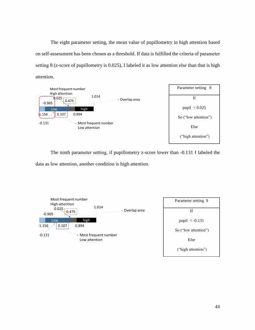
The eight parameter setting, the mean value of pupillometry in high attention based

on self-assessment has been chosen as a threshold. If data is fulfilled the criteria of parameter

setting 8 (z-score of pupillometry is 0.025), I labeled it as low attention else than that is high

attention.

The ninth parameter setting, if pupillometry z-score lower than -0.131 I labeled the

data as low attention, another condition is high attention.

Parameter setting 8

If

pupil < 0.025


Else


Parameter setting 9

If

pupil < -0.131


Else


44

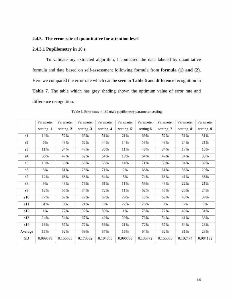
2.4.3. The error rate of quantitative for attention level

2.4.3.1 Pupillometry in 10 s

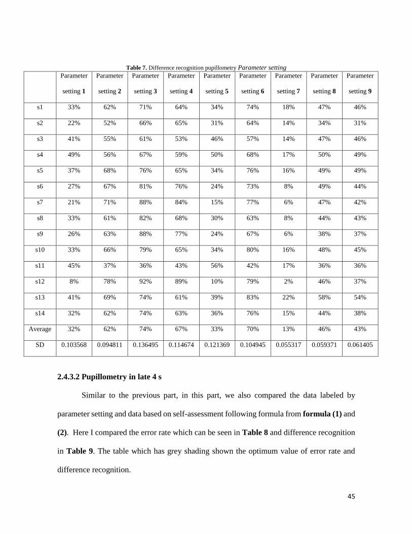
To validate my extracted algorithm, I compared the data labeled by quantitative

formula and data based on self-assessment following formula from formula (1) and (2).

Here we compared the error rate which can be seen in Table 6 and difference recognition in

Table 7. The table which has grey shading shown the optimum value of error rate and

difference recognition.

Table 6. Error rates in 180 trials pupillometry parameter setting

Parameter

setting 1

Parameter

setting 2

Parameter

setting 3

Parameter

setting 4

Parameter

setting 5

Parameter

setting 6

Parameter

setting 7

Parameter

setting 8

Parameter

setting 9

s1 14% 52% 66% 51% 21% 69% 52% 31% 31%

s2 6% 43% 62% 44% 14% 58% 43% 24% 21%

s3 11% 34% 47% 36% 11% 48% 34% 17% 16%

s4 36% 47% 62% 54% 19% 64% 47% 34% 33%

s5 13% 56% 68% 56% 14% 71% 56% 34% 32%

s6 5% 61% 78% 71% 2% 68% 61% 36% 29%

s7 12% 68% 88% 84% 5% 74% 68% 41% 36%

s8 9% 48% 76% 61% 11% 56% 48% 22% 21%

s9 12% 56% 84% 72% 11% 62% 56% 28% 24%

s10 27% 62% 77% 62% 29% 78% 62% 43% 39%

s11 31% 9% 21% 8% 27% 26% 9% 5% 9%

s12 1% 77% 92% 89% 1% 78% 77% 40% 31%

s13 24% 54% 67% 49% 29% 76% 54% 41% 38%

s14 16% 57% 72% 56% 21% 72% 57% 34% 28%

Average 15% 52% 69% 57% 15% 64% 52% 31% 28%

SD 0.099599 0.155085 0.173582 0.194805 0.090068 0.135772 0.155085 0.102474 0.084192

45

Table 7. Difference recognition pupillometry Parameter setting Parameter

setting 1

Parameter

setting 2

Parameter

setting 3

Parameter

setting 4

Parameter

setting 5

Parameter

setting 6

Parameter

setting 7

Parameter

setting 8

Parameter

setting 9

s1 33% 62% 71% 64% 34% 74% 18% 47% 46%

s2 22% 52% 66% 65% 31% 64% 14% 34% 31%

s3 41% 55% 61% 53% 46% 57% 14% 47% 46%

s4 49% 56% 67% 59% 50% 68% 17% 50% 49%

s5 37% 68% 76% 65% 34% 76% 16% 49% 49%

s6 27% 67% 81% 76% 24% 73% 8% 49% 44%

s7 21% 71% 88% 84% 15% 77% 6% 47% 42%

s8 33% 61% 82% 68% 30% 63% 8% 44% 43%

s9 26% 63% 88% 77% 24% 67% 6% 38% 37%

s10 33% 66% 79% 65% 34% 80% 16% 48% 45%

s11 45% 37% 36% 43% 56% 42% 17% 36% 36%

s12 8% 78% 92% 89% 10% 79% 2% 46% 37%

s13 41% 69% 74% 61% 39% 83% 22% 58% 54%

s14 32% 62% 74% 63% 36% 76% 15% 44% 38%

Average 32% 62% 74% 67% 33% 70% 13% 46% 43%

SD 0.103568 0.094811 0.136495 0.114674 0.121369 0.104945 0.055317 0.059371 0.061405

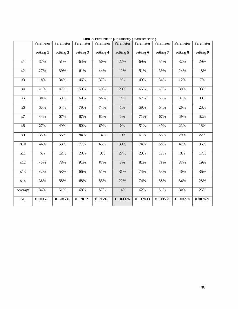
2.4.3.2 Pupillometry in late 4 s

Similar to the previous part, in this part, we also compared the data labeled by

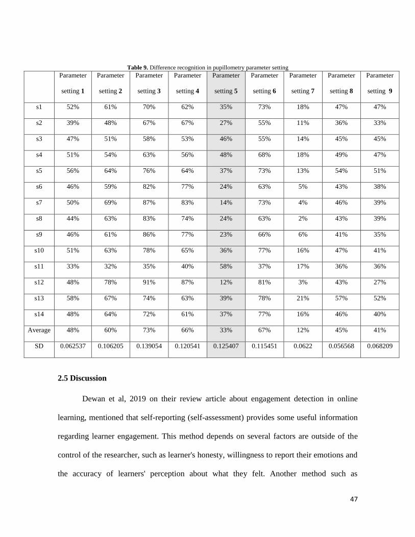
parameter setting and data based on self-assessment following formula from formula (1) and

(2). Here I compared the error rate which can be seen in Table 8 and difference recognition

in Table 9. The table which has grey shading shown the optimum value of error rate and

difference recognition.

46

Table 8. Error rate in pupillometry parameter setting

Parameter

setting 1

Parameter

setting 2

Parameter

setting 3

Parameter

setting 4

Parameter

setting 5

Parameter

setting 6

Parameter

setting 7

Parameter

setting 8

Parameter

setting 9

s1 37% 51% 64% 50% 22% 69% 51% 32% 29%

s2 27% 39% 61% 44% 12% 51% 39% 24% 18%

s3 18% 34% 46% 37% 9% 49% 34% 12% 7%

s4 41% 47% 59% 49% 20% 65% 47% 39% 33%

s5 38% 53% 69% 56% 14% 67% 53% 34% 30%

s6 33% 54% 79% 74% 1% 59% 54% 29% 23%

s7 44% 67% 87% 83% 3% 71% 67% 39% 32%

s8 27% 49% 80% 69% 0% 51% 49% 23% 18%

s9 35% 55% 84% 74% 10% 61% 55% 29% 22%

s10 46% 58% 77% 63% 30% 74% 58% 42% 36%

s11 6% 12% 20% 9% 27% 29% 12% 8% 17%

s12 45% 78% 91% 87% 3% 81% 78% 37% 19%

s13 42% 53% 66% 51% 31% 74% 53% 40% 36%

s14 38% 58% 68% 55% 22% 74% 58% 36% 28%

Average 34% 51% 68% 57% 14% 62% 51% 30% 25%

SD 0.109541 0.148534 0.178121 0.195941 0.104326 0.132898 0.148534 0.100278 0.082621

47

Table 9. Difference recognition in pupillometry parameter setting Parameter

setting 1

Parameter

setting 2

Parameter

setting 3

Parameter

setting 4

Parameter

setting 5

Parameter

setting 6

Parameter

setting 7

Parameter

setting 8

Parameter

setting 9

s1 52% 61% 70% 62% 35% 73% 18% 47% 47%

s2 39% 48% 67% 67% 27% 55% 11% 36% 33%

s3 47% 51% 58% 53% 46% 55% 14% 45% 45%

s4 51% 54% 63% 56% 48% 68% 18% 49% 47%

s5 56% 64% 76% 64% 37% 73% 13% 54% 51%

s6 46% 59% 82% 77% 24% 63% 5% 43% 38%

s7 50% 69% 87% 83% 14% 73% 4% 46% 39%

s8 44% 63% 83% 74% 24% 63% 2% 43% 39%

s9 46% 61% 86% 77% 23% 66% 6% 41% 35%

s10 51% 63% 78% 65% 36% 77% 16% 47% 41%

s11 33% 32% 35% 40% 58% 37% 17% 36% 36%

s12 48% 78% 91% 87% 12% 81% 3% 43% 27%

s13 58% 67% 74% 63% 39% 78% 21% 57% 52%

s14 48% 64% 72% 61% 37% 77% 16% 46% 40%

Average 48% 60% 73% 66% 33% 67% 12% 45% 41%

SD 0.062537 0.106205 0.139054 0.120541 0.125407 0.115451 0.0622 0.056568 0.068209

2.5 Discussion

Dewan et al, 2019 on their review article about engagement detection in online

learning, mentioned that self-reporting (self-assessment) provides some useful information

regarding learner engagement. This method depends on several factors are outside of the

control of the researcher, such as learner's honesty, willingness to report their emotions and

the accuracy of learners' perception about what they felt. Another method such as

48

observational also has some limitations such as the observation metric that may not always

be related to engagement but tend to measure compliance and willingness to adhere to rules

rather than engagement. Which this statement they quoted from Whitehill et al, 2014. They

mentioned very short response times on easy questions indicates that the learners are not

engaged and are simply giving random answers without effort. On the other hand, our

research proposed a new solution for this detection. Dewan et al, 2019, also mentioned

method by using physiological data such as eye movement, neurological data tend to not

interrupt learners in the engagement detection process. To do so, I try to compare the data

from 3 methods of engagement or attention levels such as behavior, observation, and

objective performance. And from those data, I found the difference evaluation between self-

assessment and objective behavior and observations are less than 21%.

Because in my study the cognitive tasks have several levels, I investigated the effect

of my task design toward pupillometry during high attention. I only analyze high attention in

each task because mostly data from self-assessment fill high attention, so data in low attention

could not be used. I did ANOVA analysis on 13 participants from the data that has been used

in this study (14 participants), one participant ass excluded because, in one task condition,

the participants' self-assessment mentioned that participants only feel low attention. I got

F=0.13754, P-value 0.871978 in arithmetic in 4 digits, 5 digits 6 digits. Forward digit span

F=0.16545, P-value 0.848148. Backward digit span F=0.056075, P-value 0.94555. There is

no significant difference in each task with P >0.05 similar to my previous publication

(Zennifa et al, 2018). This could happen because even though my task contains multiple

levels, the level did not need different effort and easy to be done. Other researcher mentioned

49

that after 6 digit span, adult pupillometry continue to dilate and children begin to constrict.

(Johnson et al., 2014). Figure 12 showed the pupillometry activity in each task.

Figure 12. Pupillometry activity based on tasks (one participant)

I investigated attention gaze maps from all participants during experiments and

generated the figure by Ogama (Voßkühler, A., (2009). I decided to not use gaze position in

further data analysis for attention level evaluation because all participants look at the center

of the monitor as showed in Figure 13. It has also happened because my stimulus has been

appeared in the center of the monitor. So, investigating attention states based on gaze position

is inappropriate in this study.

50

Figure 13. Heat map of the gaze attention from all participants analyzed by using the Ogama unit in pixel.

In my experiment, the encoding time is 10 seconds. Experiment for attention with

encoding time at least 10 seconds also practiced by another researcher (Langner et al, 2013).

They mentioned that 10 s become the cut off a rather conservative choice and roughly

considered as sustained allocation of attention. In our study, 10 s encoding time has been also

chosen because this data will be used as data labeling for EEG, ECG, NIRS which ECG

features commonly can be analyzed at least in 10 s.

Even though my eye tracking system has frequency sampling up to 60 Hz, the pupil

size still can be analyzed. Other research compares the ability of eye tracking with other and

higher frequency sampling, it is still reliable for pupillometry (Dalmeijer, 2014), EOG

records eye movements by measuring electrical potential differences between two electrodes.

This takes advantage of the fact that the human eye is an electrical dipole consisting of a

positively charged cornea and a negatively charged retina, first discovered by Schott in 1922

( Anina et al 2016; ). So, distinguish is it blinks cause sleepiness or because of attention.

51

Blinks last from 80 ms to 500 ms. If eyelid closure were bigger than 500 ms it is considered

as microsleep episodes (Benedetto et al, 2014).

In my study, I analyzed pupillometry in the temporal analysis. My research showed

that pupillometry is higher on high attention rather than low attention. (Kang et al 2014),

mentioned that pupil dilations are capable of indexing information changes independent of

low-level visual changes (luminance). They proved that the change of pupil dilation is not

only because of the change of light but also because of the change in information. (Hartmann

et al, 2014, Naber et al, 2013) Introduced pupillometry could reflect visual attention. So, the

phenomena of changing activities in my study, it also could be because of the attention

activities.

Specifically, my research showed that the last 4 second has significantly different.

This could have happened because pupillometry is a correlation with a temporal event. Winn

et al (Winn et al, 2018) mentioned that timing is an essential part of understanding listening

effort because speech demands rapid auditory encoding as well as cognitive processing

distributed over time, rather than being deployed all at once at the end of a stimulus. The

effort might not be uniformly distributed over a perceptual event, and pupillometry measures

have the benefit of showing a change in dilation at different time landmarks. In a study

conducted by (Koenig, Uengoer, et al 2017), there was increased pupil dilation in early stages

of attention to consistently reinforced learning cues, while in later stages of learning when

those cues did not demand as much attention, relatively larger pupil dilations were observed

for ambiguous or unreinforced cues. The pupillary response was associated with a strategic

shift in attention in a goal-directed task. Karatekin, Couperous, and Marcus (2004) measured

52

significantly larger pupil dilations in conditions of divided attention in a dual-task experiment

conducted to distinguish performance accuracy and efficiency (stated as "the costs of that

performance in the mental effort").

Generally, blink will appear in an interval of 2–10 seconds and actual rates vary by

individual averaging around 10 blinks per minute in a laboratory setting. However, when the

eyes are focused on an object for an extended time, such as when reading, the rate of blinking

decreases to about 3 to 4 times per minute (Bentivoglio et al., 2004). They measured the

normal blink rate variations with behavioral tasks in 150 healthy volunteers, they found that

blink rates during conversation are higher than resting and higher than reading. Blink rates

higher in resting rather than reading was also reported by Paprocki et al, 2017. In their

conclusion, they mentioned that eye blinks are connected to the higher cognitive process, so

blink rates could be used as a marker of dopa- and gabaminergic functioning. In the beginning

of my study, I hypothesized the difference of blink rates toward attention level can be

distinguished. But unfortunately, I did not find significant difference of blink rates data. I

suspected it happened because the trials time in this study is too short to make blink rates has

significant difference.

In my knowledge, this study is the first study that tries to find the parameter setting

of pupillometry to be used for attention level evaluation. The background of this study is

because there is no explanation of former study (Zennifa et al 2018) of the usage parameter

settings in pupillometry if Z score bigger than 0 and blink rates Z score lower than 0 will be

labeled as high attention and low attention is the opposite way. So, I continue to investigate

how to find the explanation of parameter settings in attention level evaluation by using

53

eyetracking information. Extended study (Zennifa et al 2019) tried to developed quantitative

algorithm of blink rates and pupillometry for labelling method in supervised machine

learning. But in the end, I consider to not use blink rates as parameter setting because there

is no significant difference in 10 second. Other pupillometry research in attention (Karatekin

et al., 2007; Tsukahara et al., 2016; Hartmann et al, 2014; Geva et al., 2013; Unsworth et al.,

2017 a&b; Piquado et al., 2010) did not investigate the threshold for attention level but just

investigate the effect of attention and cognitive toward pupillometry. I used self-assessment

to validating our data after investigating the error rate and difference recognition compare

with other attention level evaluation methods (Objective performance, an observation in

which the result of error rate is less than 21%. Based on my comparison, I found that

threshold with z-score within a specific range (-0.965 ≤ pupil ≤ 1.014) as high attention.

2.6 Conclusion

In this chapter, I compared the self-assessment method with other attention level

detection methods (observation and objective performance) to check the difference value of

evaluation on those methods. I got a different error of self-assessment compared with other

methods lower than 21%. After that, I investigated the effect of attention level based on self-

assessment to blink rates and pupillometry. I found that pupillometry in low attention is

smaller than high attention, especially in the last 4 seconds. I extracted the pupillometry

activity in the last 4 seconds and 10 seconds into 9 algorithms each. After doing several

experimental procedures, I chose parameter setting with a percentage of error of less than

15% and a different error 35 % compare with self-assessment as future labeling method.

54

Parameter setting which has been selected is when z-score within a specific range (-0.965 ≤

pupil ≤ 1.014) as high attention, other that range, will be classified as low attention.

55

Chapter 3. Application of new labeling in EEG-ECG-NIRS

3.1. Abstract

In this chapter, I introduce the implementation of new labelling method in a low-

density hybrid system for attention level evaluation. I used a two-electrode wireless EEG, a

wireless ECG, and a NIRS with two wireless channels to measure attention level during

during backward digit span, forward digit span and arithmetic. High attention will be labelled

to data which has pupillometry z-score within specific range (-0.965 ≤ pupil ≤ 1.014) and

another that range, will be classified as low attention.

By using CFS+kNN algorithm, my result showed the accuracy system of EEG-ECG-

NIRS (83.33± 5.95%) has the highest accuracy compare with EEG (81.90± 4.69%), ECG

(82.51±3.57%), NIRS (78.37±7.12%). Algorithm CFS+kNN also shown highest

performance compare with other methods such as CFS+SVM (55.49± 27.89%), kNN

(80.84± 3.88%) and SVM (55.88± 13.14%).

3.2 Materials and method

3.2.1 Participants

In my experiment, 24 participants were Kyushu University students, with ages

ranging from 21 to 28 (24.25 ± 2.3). All participants had a normal visual function and were

free of disability. Among them, 21 were right-handed, one participant was ambidextrous, and

two participants were left-handed. The participants were instructed not to consume any

caffeine 2 hours before the experiment because it could affect the HRV (Martínez-Sellés et

al, 2013; Oliveira et al, 2017). The study was conducted following the ethical principles of

56

Kyushu University and the Declaration of Helsinki. Written informed consent was obtained

from each participant before the experiment as showed on Appendix 2.

3.2.2 Experiment task

The experiment was done at between 10:30 am and 1:30 pm in a dimly lit room. We

also recorded the behavior activities of the participants using a webcam camera (Logicool

C270, Logitech, city, Switzerland), put in front of the participant’s face.

Three types of attention tasks were used: a backward digit span (BDS) (Jensen et al., 1975;

Cullum., 1998; Berka et al 2007; Zennifa et al., 2018; Zennifa et al., 2019; Rosenthal et al,

2006), a forward digit span (FDS) (Jensen et al., 1975; Cullum., 1998; Berka et al 2007,

Zennifa et al., 2018; Zennifa et al., 2019; Rosenthal et al, 2006), and an arithmetic (Zennifa

et al, 2018). These tasks consist of three levels. Level one consisted of a series of 30 sets of

four digits, level two: 30 sets of five digits and level three: six digits. Most of the questions

in this experiment were relatively simple and did not require any prerequisite knowledge or

specific skills. However, a good level of attention and alertness was required to avoid making

easy mistakes because the response time was limited to 20 s. Each trial started with the

presentation of a central, white fixation dot on a dark background until the participant's eyes

could be accepted by the eye tracker. Next, cognitive questions (i.e., encoding session) would

appear for 10 s and the participant was instructed to respond within 20 s. All cognitive tasks

were counterbalanced. The measurement of EEG-ECG-NIRS-EOG and Eye tracking was

recorded after the practice session finished.

57

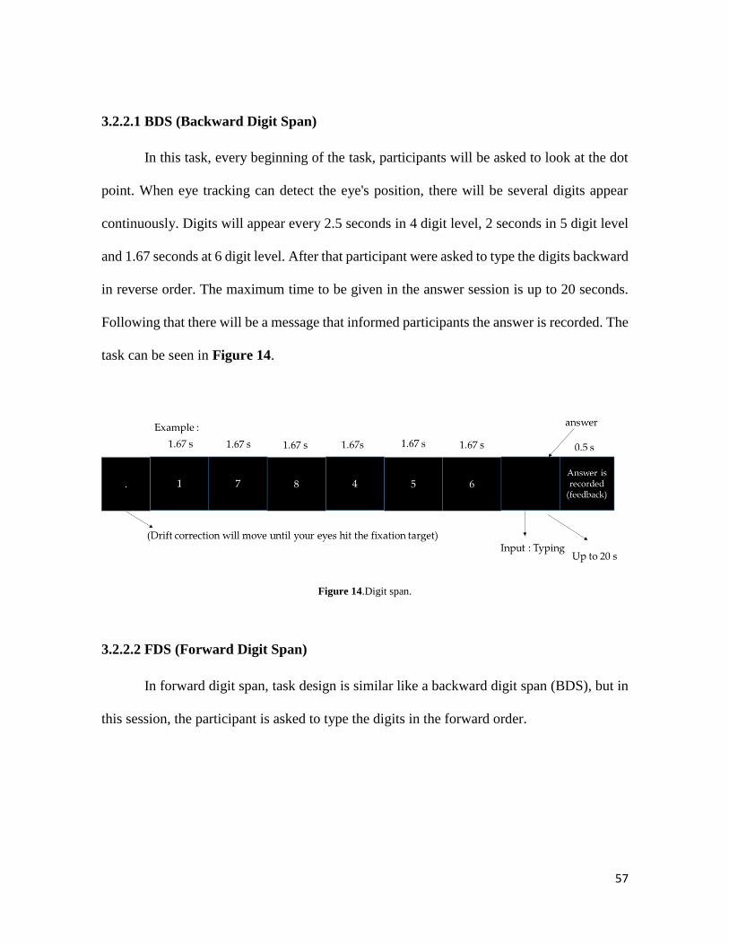
3.2.2.1 BDS (Backward Digit Span)

In this task, every beginning of the task, participants will be asked to look at the dot

point. When eye tracking can detect the eye's position, there will be several digits appear

continuously. Digits will appear every 2.5 seconds in 4 digit level, 2 seconds in 5 digit level

and 1.67 seconds at 6 digit level. After that participant were asked to type the digits backward

in reverse order. The maximum time to be given in the answer session is up to 20 seconds.

Following that there will be a message that informed participants the answer is recorded. The

task can be seen in Figure 14.

Figure 14.Digit span.

3.2.2.2 FDS (Forward Digit Span)

In forward digit span, task design is similar like a backward digit span (BDS), but in

this session, the participant is asked to type the digits in the forward order.

58

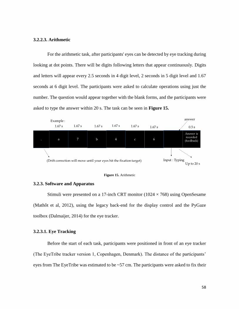
3.2.2.3. Arithmetic

For the arithmetic task, after participants' eyes can be detected by eye tracking during

looking at dot points. There will be digits following letters that appear continuously. Digits

and letters will appear every 2.5 seconds in 4 digit level, 2 seconds in 5 digit level and 1.67

seconds at 6 digit level. The participants were asked to calculate operations using just the

number. The question would appear together with the blank forms, and the participants were

asked to type the answer within 20 s. The task can be seen in Figure 15.

Figure 15. Arithmetic

3.2.3. Software and Apparatus

Stimuli were presented on a 17-inch CRT monitor (1024 × 768) using OpenSesame

(Mathôt et al, 2012), using the legacy back-end for the display control and the PyGaze

toolbox (Dalmaijer, 2014) for the eye tracker.

3.2.3.1. Eye Tracking

Before the start of each task, participants were positioned in front of an eye tracker

(The EyeTribe tracker version 1, Copenhagen, Denmark). The distance of the participants’

eyes from The EyeTribe was estimated to be ~57 cm. The participants were asked to fix their

59

heads on a chin rest. Eight participants were successfully calibrated in the 60 Hz mode while

three participants were successfully calibrated in the 30 Hz mode. In this study, we calibrated

and validated the eye tracking system to each participant using a nine-point dot matrix. After

validation, the eye tracker that had been embedded with the OpenSesame software labeled

each calibration point with the error in the degree of the visual angle between the calibrated

and validated measures. If the calibration points do not exceed 1°[deg] and the greatest single

point error does not exceed 1°, the process would continue. Before each trial, a one-point eye

tracker recalibration was performed.

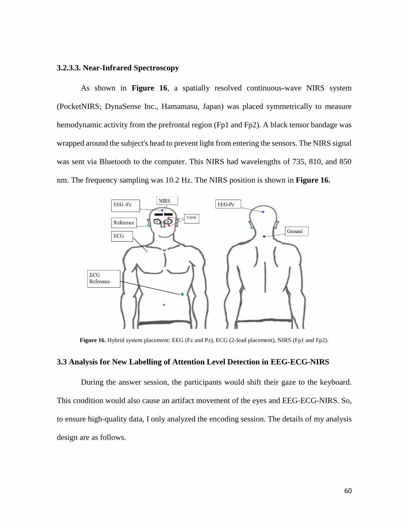
3.2.3.2. Electrophysiology

In this study, EEG, and ECG (Polymate Mini AP 108, Miyuki Giken Co., Ltd.,

Kasugai-city, Japan) signals were sent by Bluetooth to a computer. The frequency of

sampling was 500 Hz. To evaluate attention level during a cognitive task, we recorded EEG

at the Fz and Pz, referenced at A1. These areas are highly correlated in cognitive activities

(Culham et al., 2006; Reynolds et al., 2016; Chayer et al., 2001). The ECG was recorded on

the chest (2-lead placement) (Stikic at al., 2014;, Zennifa et al.,2015; Iramina et al., 2010).

We chose this position for the ECG to reduce the effect of artifact movements when the

participant responded to the tasks. We also put two electrodes for a vertical EOG as shown

in. Figure 16 shows the electrode placements. This location was chosen to detect blink

(Waters et al.,2005 ; Huang et al, .2018).

60

3.2.3.3. Near-Infrared Spectroscopy

As shown in Figure 16, a spatially resolved continuous-wave NIRS system

(PocketNIRS; DynaSense Inc., Hamamasu, Japan) was placed symmetrically to measure

hemodynamic activity from the prefrontal region (Fp1 and Fp2). A black tensor bandage was

wrapped around the subject's head to prevent light from entering the sensors. The NIRS signal

was sent via Bluetooth to the computer. This NIRS had wavelengths of 735, 810, and 850

nm. The frequency sampling was 10.2 Hz. The NIRS position is shown in Figure 16.

Figure 16. Hybrid system placement: EEG (Fz and Pz), ECG (2-lead placement), NIRS (Fp1 and Fp2).

3.3 Analysis for New Labelling of Attention Level Detection in EEG-ECG-NIRS

During the answer session, the participants would shift their gaze to the keyboard.

This condition would also cause an artifact movement of the eyes and EEG-ECG-NIRS. So,

to ensure high-quality data, I only analyzed the encoding session. The details of my analysis

design are as follows.

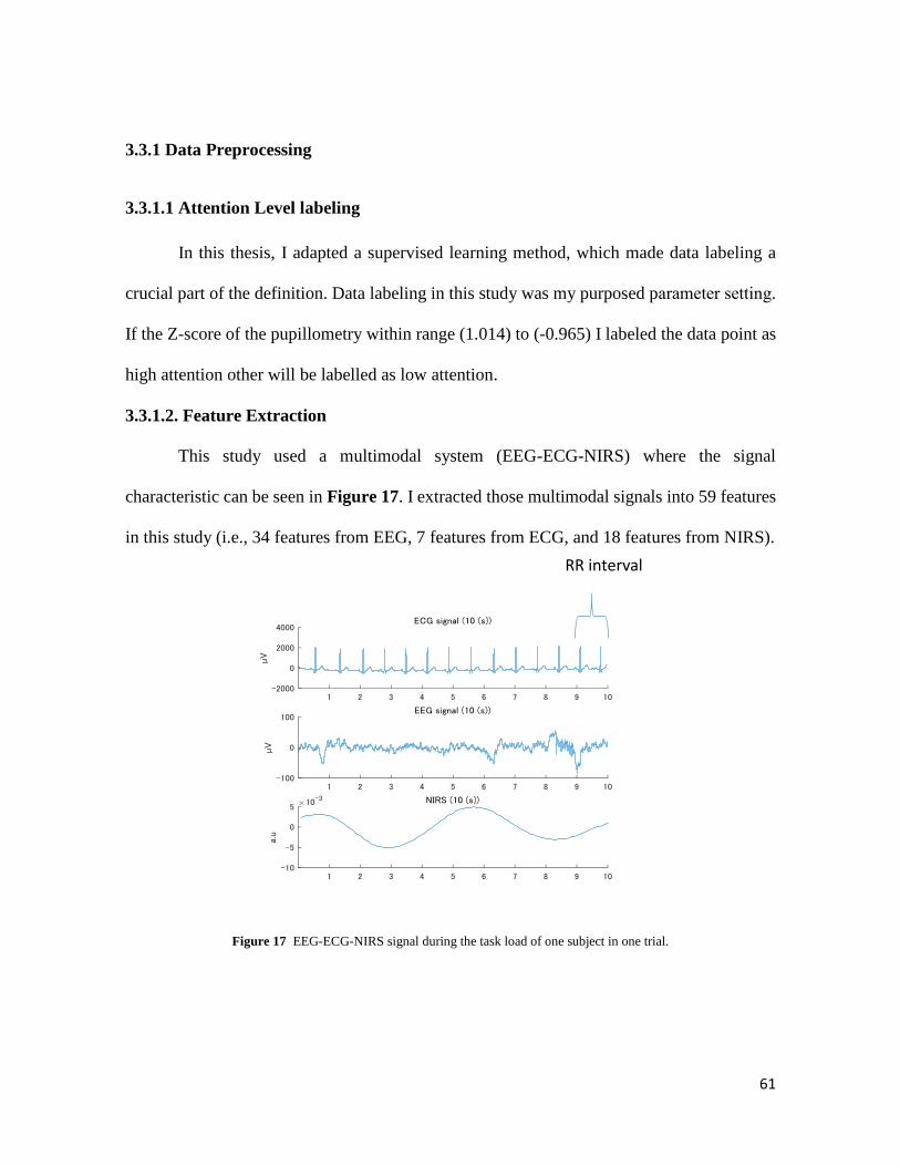
61

3.3.1 Data Preprocessing

3.3.1.1 Attention Level labeling

In this thesis, I adapted a supervised learning method, which made data labeling a

crucial part of the definition. Data labeling in this study was my purposed parameter setting.

If the Z-score of the pupillometry within range (1.014) to (-0.965) I labeled the data point as

high attention other will be labelled as low attention.

3.3.1.2. Feature Extraction

This study used a multimodal system (EEG-ECG-NIRS) where the signal

characteristic can be seen in Figure 17. I extracted those multimodal signals into 59 features

in this study (i.e., 34 features from EEG, 7 features from ECG, and 18 features from NIRS).

Figure 17 EEG-ECG-NIRS signal during the task load of one subject in one trial.

RR interval

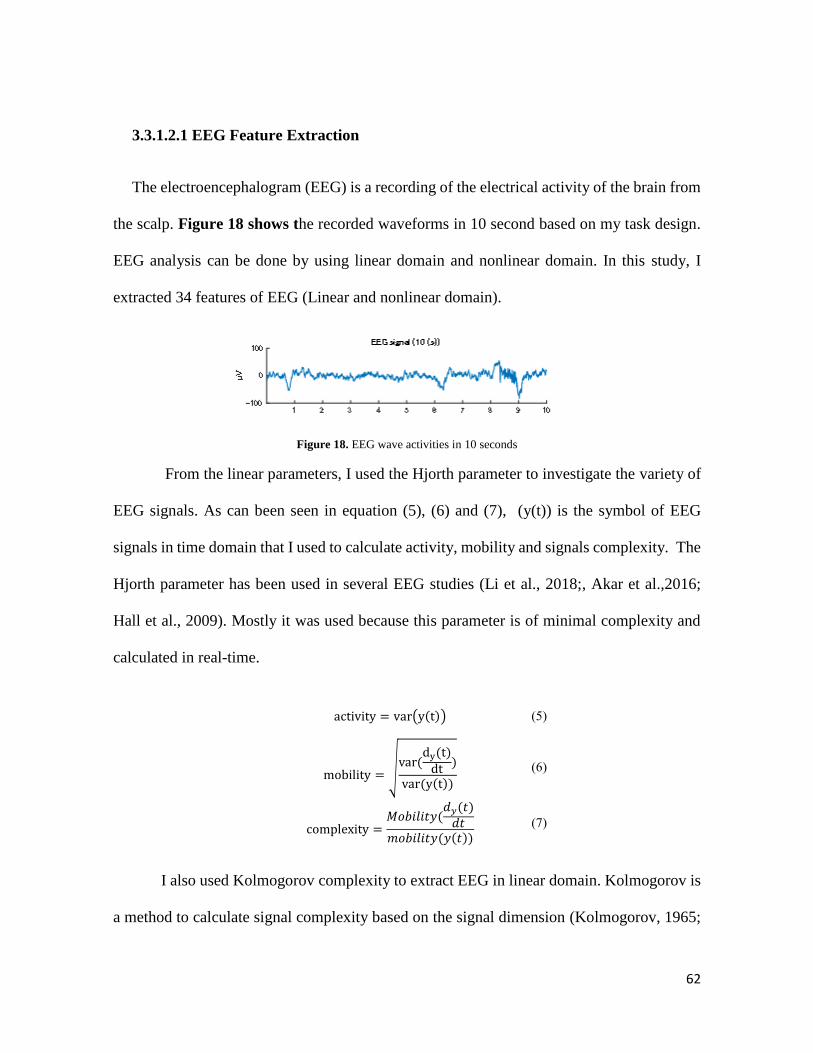
62

3.3.1.2.1 EEG Feature Extraction

The electroencephalogram (EEG) is a recording of the electrical activity of the brain from

the scalp. Figure 18 shows the recorded waveforms in 10 second based on my task design.

EEG analysis can be done by using linear domain and nonlinear domain. In this study, I

extracted 34 features of EEG (Linear and nonlinear domain).

Figure 18. EEG wave activities in 10 seconds

From the linear parameters, I used the Hjorth parameter to investigate the variety of

EEG signals. As can been seen in equation (5), (6) and (7), (y(t)) is the symbol of EEG

signals in time domain that I used to calculate activity, mobility and signals complexity. The

Hjorth parameter has been used in several EEG studies (Li et al., 2018;, Akar et al.,2016;

Hall et al., 2009). Mostly it was used because this parameter is of minimal complexity and

calculated in real-time.

I also used Kolmogorov complexity to extract EEG in linear domain. Kolmogorov is

a method to calculate signal complexity based on the signal dimension (Kolmogorov, 1965;

activity = var(y(t)) (5)

mobility = √var(dy(t)

dt)

var(y(t))

(6)

complexity =𝑀𝑜𝑏𝑖𝑙𝑖𝑡𝑦(

𝑑𝑦(𝑡)𝑑𝑡

𝑚𝑜𝑏𝑖𝑙𝑖𝑡𝑦(𝑦(𝑡))

(7)

63

Lui et al., 2015). Where φ represents a universal computer, p represents a program and x

represent a string. I extracted Kolmogorov complexity by using library which provided in

mat lab (Faul, s 2015).

𝐾𝜑(𝑥) = {𝑚𝑖𝑛𝜑(𝑝)=𝑥𝑙(𝑝)} (8)

The EEG signal was calculated in 10 s windows. Wavelet Daubechies 8 was applied

to get the value of power spectral density. Because I used 500 Hz frequency sampling EEG,

I need to decide the decomposition level wavelet. By following the Nyquist rule, half the

frequencies should be removed. Low pass filter g and high pass filter h with half cut off

frequency. Figure 19 shows wavelet transform decomposition which seven levels.

CD5

CD6

CA7

CA6 CD7

CA5

g(n)

CA4

CD4

EEG

signal FS = 500

Hz

g(n)

h(n)

Gamma

32-64 Hz

g(n)

h(n) g(n)

h(n)

h(n)

Beta

16-32 Hz

Alpha

8-12 Hz

Theta

8-12 Hz

Delta

8-12 Hz

Figure 19. Seven levels EEG signal decomposition using discrete wavelet transform.

64

After obtaining the power of the EEG oscillation, I also calculated the maximum

power of EEG and power density integral of EEG which can be seen in appendix 6. Also the

relative power of each band (i.e., theta (θ) (Equation (13)), alpha (Equation (14)), and beta

(β), (Equation (15), and gamma (γ) (Equation (16)) were computed from each electrode as

this following equations:

power θ = ((D7.^2))/length(D7); (9)

power α = ((D6.^2))/length(D6); (10)

power β = ((D5.^2))/length(D5); (11)

power γ = ((D4.^2))/length(D4); (12)

Relative θ = (power θ)/(power θ + power α + power β + power γ) (13)

Relative α = (power α)/(power θ + power α + power β + power γ) (14)

Relative β = (power β)/(power θ + power α + power β + power γ) (15)

Relative γ = (power γ)/(power θ + power α + power β + power γ) (16)

I calculated EEG power spectral entropy after calculated EEG power spectral density

by using pwelch function from Matlab library and applied entropy calculation by using

Matlab library Appendix 6. The calculation is based on Shannon formula (equation 17) I

calculated power spectral entropy to investigated correlation nonlinear features toward

attention level.

𝑆𝐸𝑛 = −𝑘 ∑ 𝑃𝑠�̂�(𝑓)𝑙𝑜𝑔𝑃𝑠�̂�(𝑓)𝑓=45𝑓=0.5 (17)

Where k=1 and the basis f log is 10. The symbol of f means frequency, and the

frequency was to be set in range 0.5 Hz to 45 Hz.

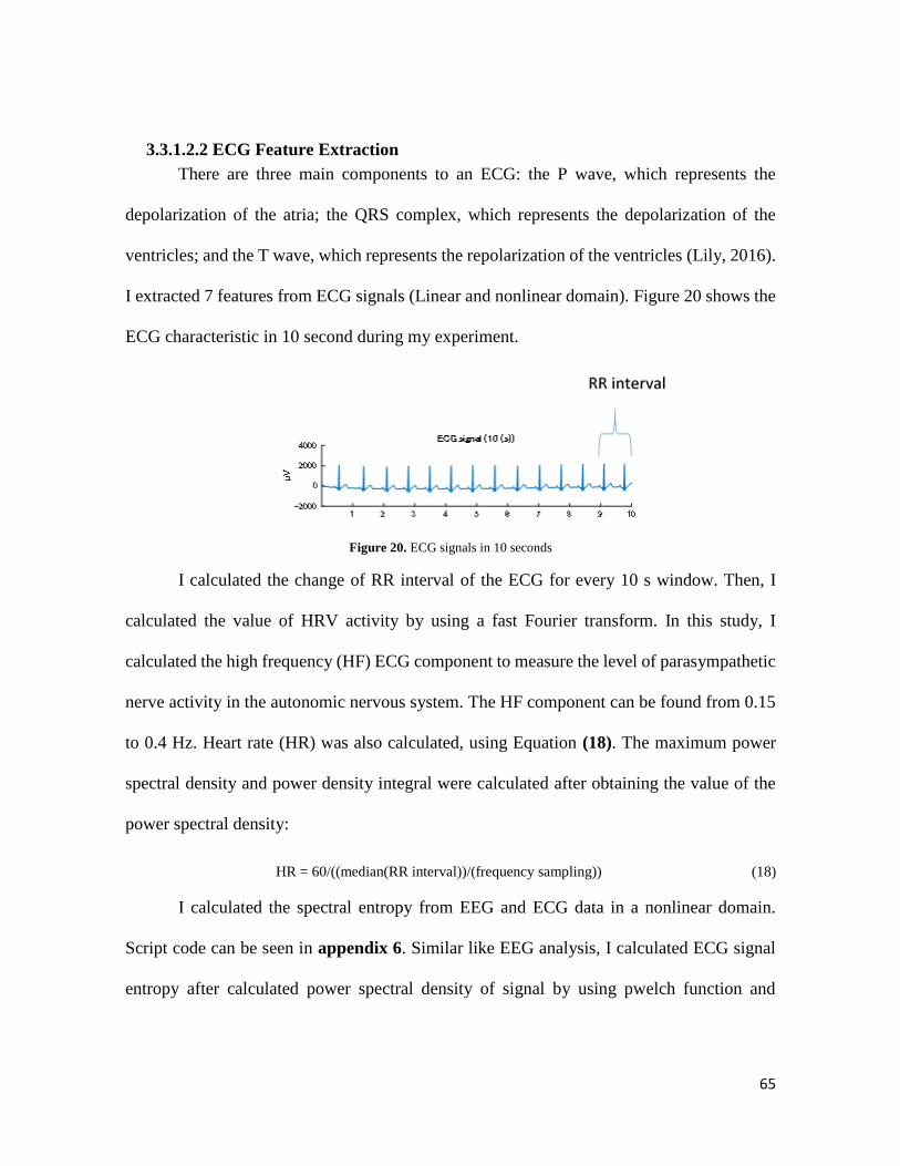
65

3.3.1.2.2 ECG Feature Extraction

There are three main components to an ECG: the P wave, which represents the

depolarization of the atria; the QRS complex, which represents the depolarization of the

ventricles; and the T wave, which represents the repolarization of the ventricles (Lily, 2016).

I extracted 7 features from ECG signals (Linear and nonlinear domain). Figure 20 shows the

ECG characteristic in 10 second during my experiment.

Figure 20. ECG signals in 10 seconds

I calculated the change of RR interval of the ECG for every 10 s window. Then, I

calculated the value of HRV activity by using a fast Fourier transform. In this study, I

calculated the high frequency (HF) ECG component to measure the level of parasympathetic

nerve activity in the autonomic nervous system. The HF component can be found from 0.15

to 0.4 Hz. Heart rate (HR) was also calculated, using Equation (18). The maximum power

spectral density and power density integral were calculated after obtaining the value of the

power spectral density:

HR = 60/((median(RR interval))/(frequency sampling)) (18)

I calculated the spectral entropy from EEG and ECG data in a nonlinear domain.

Script code can be seen in appendix 6. Similar like EEG analysis, I calculated ECG signal

entropy after calculated power spectral density of signal by using pwelch function and

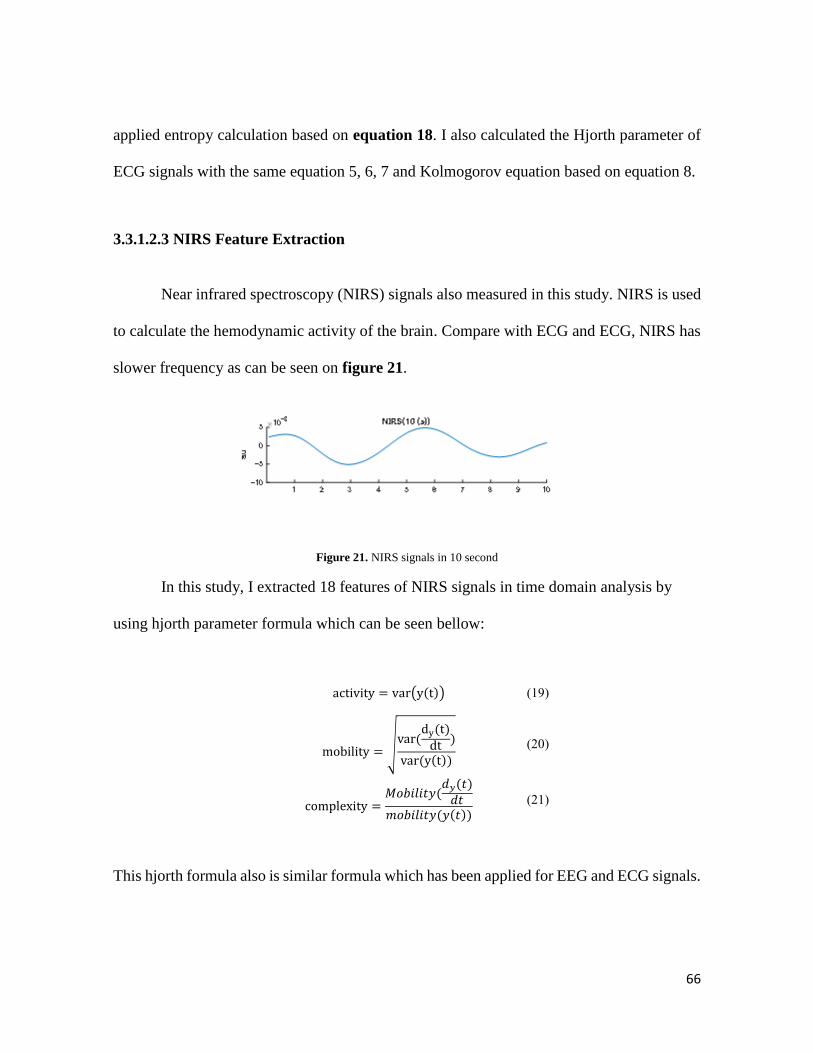
66

applied entropy calculation based on equation 18. I also calculated the Hjorth parameter of

ECG signals with the same equation 5, 6, 7 and Kolmogorov equation based on equation 8.

3.3.1.2.3 NIRS Feature Extraction

Near infrared spectroscopy (NIRS) signals also measured in this study. NIRS is used

to calculate the hemodynamic activity of the brain. Compare with ECG and ECG, NIRS has

slower frequency as can be seen on figure 21.

Figure 21. NIRS signals in 10 second

In this study, I extracted 18 features of NIRS signals in time domain analysis by

using hjorth parameter formula which can be seen bellow:

This hjorth formula also is similar formula which has been applied for EEG and ECG signals.

activity = var(y(t)) (19)

mobility = √var(dy(t)

dt)

var(y(t))

(20)

complexity =𝑀𝑜𝑏𝑖𝑙𝑖𝑡𝑦(

𝑑𝑦(𝑡)𝑑𝑡

𝑚𝑜𝑏𝑖𝑙𝑖𝑡𝑦(𝑦(𝑡))

(21)

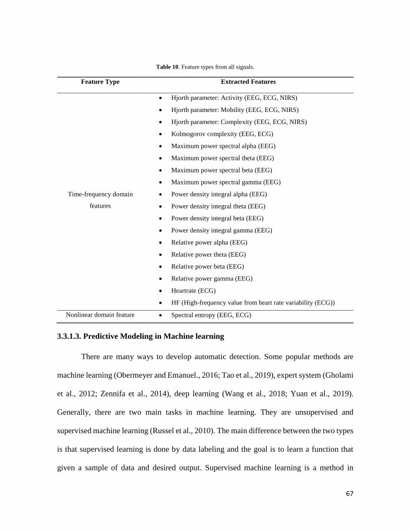
67

Table 10. Feature types from all signals.

Feature Type Extracted Features

Time-frequency domain

features

Hjorth parameter: Activity (EEG, ECG, NIRS)

Hjorth parameter: Mobility (EEG, ECG, NIRS)

Hjorth parameter: Complexity (EEG, ECG, NIRS)

Kolmogorov complexity (EEG, ECG)

Maximum power spectral alpha (EEG)

Maximum power spectral theta (EEG)

Maximum power spectral beta (EEG)

Maximum power spectral gamma (EEG)

Power density integral alpha (EEG)

Power density integral theta (EEG)

Power density integral beta (EEG)

Power density integral gamma (EEG)

Relative power alpha (EEG)

Relative power theta (EEG)

Relative power beta (EEG)

Relative power gamma (EEG)

Heartrate (ECG)

HF (High-frequency value from heart rate variability (ECG))

Nonlinear domain feature Spectral entropy (EEG, ECG)

3.3.1.3. Predictive Modeling in Machine learning

There are many ways to develop automatic detection. Some popular methods are

machine learning (Obermeyer and Emanuel., 2016; Tao et al., 2019), expert system (Gholami

et al., 2012; Zennifa et al., 2014), deep learning (Wang et al., 2018; Yuan et al., 2019).

Generally, there are two main tasks in machine learning. They are unsupervised and

supervised machine learning (Russel et al., 2010). The main difference between the two types

is that supervised learning is done by data labeling and the goal is to learn a function that

given a sample of data and desired output. Supervised machine learning is a method in

68

machine learning by using knowing labeling methods to label the data and has the expecting

result (input-output pairs) (Stuart et al, 2010). On the contrary, unsupervised machine

learning is not based on data labeling and its goal is to infer the natural structure present

within a set of data points. Measuring human mental states based on physiological activity

has also been investigated by integrating EEG and ECG features (Stikic et al., 2014). The

unsupervised method has been applied for cognitive state recognition in that experiment.

However, the unsupervised learning requires large amounts of data to get an appropriate

pattern. Moreover, there is no method to validate the data. In our study, data labeling relied

on physiological activities. I used Weka 3.8 (Hall et al., 2009) data mining for machine

learning.

3.3.1.3.1 CFS (Correlation Based Feature selection)

The feature selector is important for reducing the time needed to find the best features

to be used in a study case (Aghajani et al., 2017; Hall et al, 1999), and it also can increase

the accuracy of classification. The CFS (correlation-based feature selection) is a simple filter

algorithm that ranks feature subsets according to a correlation-based heuristic evaluation

function (Hall, 1999). This feature selector calculates features that are highly correlated with

the class and uncorrelated with each other. Irrelevant features would be ignored because they

have a low correlation with the class. Redundant features would be screened out, as they are

highly correlated with one or more of the remaining features. The acceptance of a feature

will depend on the extent to which it predicts classes in an area if the instance space was not

already predicted by other features. Equations (18) through (21) show the calculation process:

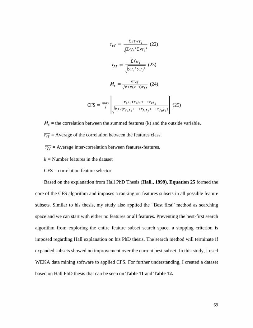
69

𝑟𝑐𝑓 = ∑ 𝑐𝑓𝑖𝑐𝑓𝑗

√∑ 𝑐𝑓𝑖2 ∑ 𝑐𝑓𝑗

2 (22)

𝑟𝑓𝑓 = ∑ 𝑓𝑖𝑓𝑗

√∑ 𝑓𝑖2 ∑ 𝑓𝑗

2 (23)

𝑀𝑠 =𝑘𝑟𝑐𝑓̅̅ ̅̅ ̅

√𝑘+𝑘(𝑘−1)𝑟𝑓𝑓̅̅ ̅̅ ̅ (24)

CFS = 𝑚𝑎𝑥𝑠

[𝑟𝑐𝑓1+𝑟𝑐𝑓2+⋯+𝑟𝑐𝑓𝑘

√𝑘+2(𝑟𝑓1𝑓2+⋯+𝑟𝑓𝑖𝑓𝑗+⋯+𝑟𝑓𝑘𝑓1)

] (25)

𝑀𝑠 = the correlation between the summed features (k) and the outside variable.

𝑟𝑐𝑓̅̅ ̅̅ = Average of the correlation between the features class.

𝑟𝑓𝑓̅̅ ̅̅ = Average inter-correlation between features-features.

k = Number features in the dataset

CFS = correlation feature selector

Based on the explanation from Hall PhD Thesis (Hall., 1999), Equation 25 formed the

core of the CFS algorithm and imposes a ranking on features subsets in all possible feature

subsets. Similar to his thesis, my study also applied the “Best first” method as searching

space and we can start with either no features or all features. Preventing the best-first search

algorithm from exploring the entire feature subset search space, a stopping criterion is

imposed regarding Hall explanation on his PhD thesis. The search method will terminate if

expanded subsets showed no improvement over the current best subset. In this study, I used

WEKA data mining software to applied CFS. For further understanding, I created a dataset

based on Hall PhD thesis that can be seen on Table 11 and Table 12.

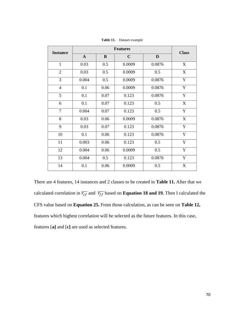
70

Table 11. Dataset example

Instance Features

Class A B C D

1 0.03 0.5 0.0009 0.0876 X

2 0.03 0.5 0.0009 0.5 X

3 0.004 0.5 0.0009 0.0876 Y

4 0.1 0.06 0.0009 0.0876 Y

5 0.1 0.07 0.123 0.0876 Y

6 0.1 0.07 0.123 0.5 X

7 0.004 0.07 0.123 0.5 Y

8 0.03 0.06 0.0009 0.0876 X

9 0.03 0.07 0.123 0.0876 Y

10 0.1 0.06 0.123 0.0876 Y

11 0.003 0.06 0.123 0.5 Y

12 0.004 0.06 0.0009 0.5 Y

13 0.004 0.5 0.123 0.0876 Y

14 0.1 0.06 0.0009 0.5 X

There are 4 features, 14 instances and 2 classes to be created in Table 11. After that we

calculated correlation in 𝑟𝑐𝑓̅̅ ̅̅ and 𝑟𝑓𝑓̅̅ ̅̅ based on Equation 18 and 19. Then I calculated the

CFS value based on Equation 25. From those calculation, as can be seen on Table 12,

features which highest correlation will be selected as the future features. In this case,

features [a] and [c] are used as selected features.

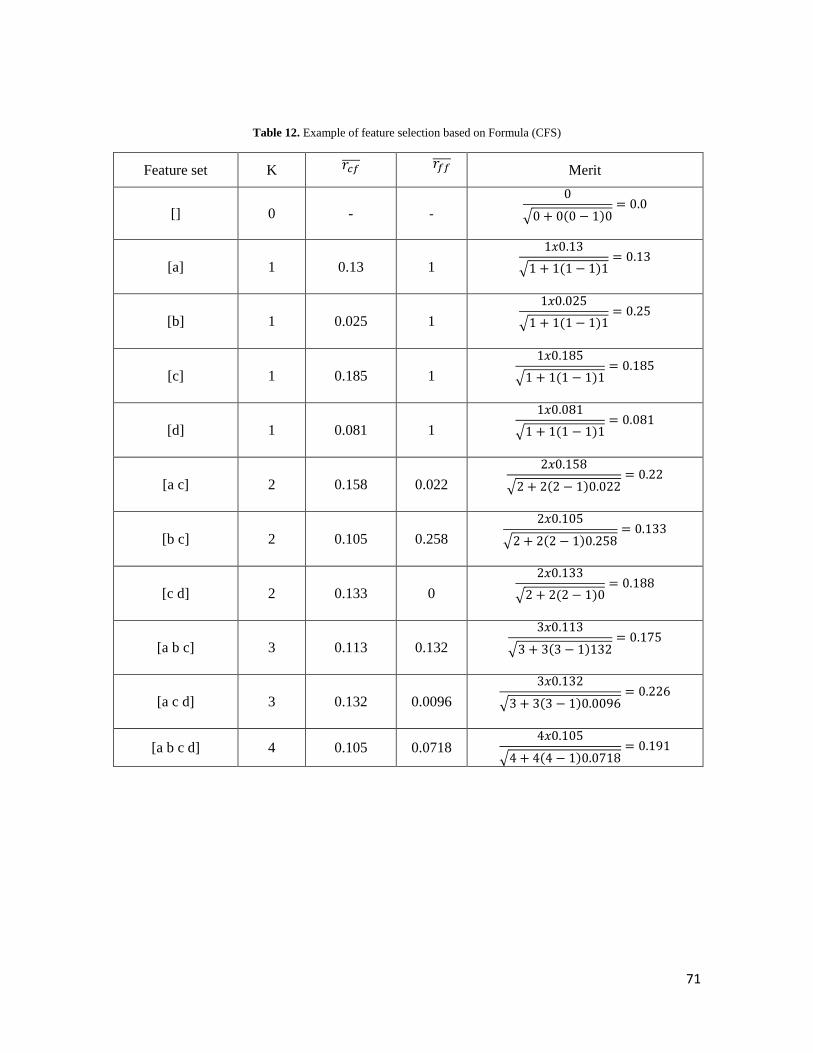
71

Table 12. Example of feature selection based on Formula (CFS)

Feature set K

Merit

[] 0 - -

0

√0 + 0(0 − 1)0= 0.0

[a] 1 0.13 1

1𝑥0.13

√1 + 1(1 − 1)1= 0.13

[b] 1 0.025 1

1𝑥0.025

√1 + 1(1 − 1)1= 0.25

[c] 1 0.185 1

1𝑥0.185

√1 + 1(1 − 1)1= 0.185

[d] 1 0.081 1

1𝑥0.081

√1 + 1(1 − 1)1= 0.081

[a c] 2 0.158 0.022

2𝑥0.158

√2 + 2(2 − 1)0.022= 0.22

[b c] 2 0.105 0.258

2𝑥0.105

√2 + 2(2 − 1)0.258= 0.133

[c d] 2 0.133 0

2𝑥0.133

√2 + 2(2 − 1)0= 0.188

[a b c] 3 0.113 0.132

3𝑥0.113

√3 + 3(3 − 1)132= 0.175

[a c d] 3 0.132 0.0096

3𝑥0.132

√3 + 3(3 − 1)0.0096= 0.226

[a b c d] 4 0.105 0.0718 4𝑥0.105

√4 + 4(4 − 1)0.0718= 0.191

𝑟𝑐𝑓̅̅ ̅̅ 𝑟𝑓𝑓̅̅ ̅̅

72

3.3.1.3.2 kNN (k Nearest Neighbor)

In this thesis, my algorithm is started by 3 multimodal input (EEG-ECG-NIRS) into one

dataset. I used WEKA data mining software and applied 10 fold cross-validation and after

that applied CFS processing on the next process. CFS calculates features-class and feature-

feature correlations and then searches the feature subset space by using the "best first search"

method. The subset with the highest correlation (Equation 25) found during the search. Then

I applied the selected features to my training and testing data, and classify the features by

using kNN (k nearest neighbor). kNN is an approach for data classification that estimates

the probability that a data point belongs to one group or another, depending on the group

membership of the data points nearest to it.

3.3.1.3.3 SVM (Support Vector Machine)

In this study, I used WEKA mining software and applied support vector machine

(SVM) polynomial as classifier. SVM is supervised learning models with associated learning

algorithms that analyze data used for classification and regression analysis (Corinna, et al

1995). One of the effectiveness of SVM depends on the selection parameter C. C is a

regularization parameter that controls the tradeoff between the achieving a low training error

and a low testing error that is the ability to generalize your classifier to unseen data. Typically,

each combination of parameter choices is checked using by accuracy performance.

3.3.1.3.4 Performance calculation

In this study, the accuracy of performance was calculated based on several variables,

such as the true positive (TP) rate. The TP rate was calculated as the proportion of cases that

73

were correctly classified as class high or low among all cases that are true of the same

corresponding class (P), i.e., the extent to which part of the classes was captured. The TP rate

value is also equivalent to the recall.

recall =𝑇𝑃

𝑃

I also calculated the false positive (FP) rate. The FP rate is the proportion of cases

that were classified as class high or low but belong to a different class, among all cases that

are not of class high or low. The precision is the proportion of the cases that truly have a class

low or high among all those that were classified as class high or low.

Precision =𝑇𝑃

𝑇𝑃 + 𝐹𝑃

The recall (i.e., sensitivity) is the fraction of relevant instances that have been

retrieved over the total amount of relevant instances. The F-measure is simply twice the time

value of the precision and recall divided by the sum value of precision and recall. I also

investigated the area under a receiver operating curve (ROC) for our performance evaluation.

F = 2𝑝𝑟𝑒𝑐𝑖𝑠𝑖𝑜𝑛. 𝑟𝑒𝑐𝑎𝑙𝑙

𝑝𝑟𝑒𝑐𝑖𝑠𝑖𝑜𝑛 + 𝑟𝑒𝑐𝑎𝑙𝑙

3.3.2. Data Management

3.3.2.1 Data Modelling

3.3.2.1.1 Hold out Method

In this process, data was separated into training set and testing set. The training aims

to to fit the model and testing data to test the modal. In this method, Data was separated into

70% data for training, 30% data for testing.

74

3.3.2.1.2 Cross validation Method (XV Method)

In this process, data set is divided into k subsets, and the holdout method is repeated

k times. Each time, one of the k subsets is used as the test set and the other k-1 subsets are

put together to form a training set. Then the average error across all k trials is computed. In

this study, the cross validation has been applied in 10 folded.

3.3.2.1.3 Leave one subject out validation (LOSOXV)

In this process, data was separated into training set and testing set. The training aims

to to fit the model and testing data to test the modal. In this method, one participant is leave

out as testing data and other used as training data. This process was repeated till all

participants finish to be tested.

3.3.2.2. Data Balancing

3.3.2.2.1 Oversampling

In this study, high attention and low attention data are an imbalance, I need to

anticipate this condition by re-sampling my data (Chicco et al, 2017). There are several ways

to re-sampling data. To make my data become balance, I applied oversampling, which means

increasing the number of minority class members in the training set. In this study,

oversampling was performed by using weka resample library. This resample library can

produces a random subsample of a dataset. The original dataset must fit entirely in memory.

The number of instances in the generated dataset may be specified. The filter can be made to

maintain the class distribution in the subsample, or to bias the class distribution toward a

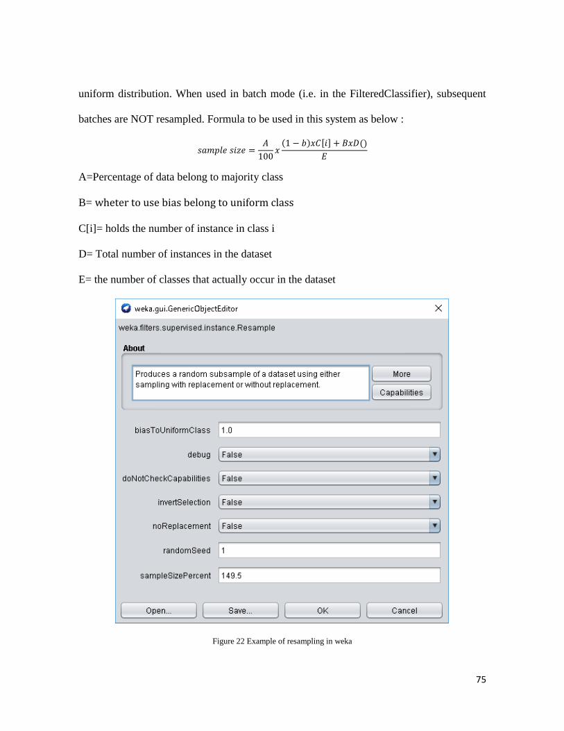
75

uniform distribution. When used in batch mode (i.e. in the FilteredClassifier), subsequent

batches are NOT resampled. Formula to be used in this system as below :

𝑠𝑎𝑚𝑝𝑙𝑒 𝑠𝑖𝑧𝑒 =𝐴

100𝑥

(1 − 𝑏)𝑥𝐶[𝑖] + 𝐵𝑥𝐷()

𝐸

A=Percentage of data belong to majority class

B= wheter to use bias belong to uniform class

C[i]= holds the number of instance in class i

D= Total number of instances in the dataset

E= the number of classes that actually occur in the dataset

Figure 22 Example of resampling in weka

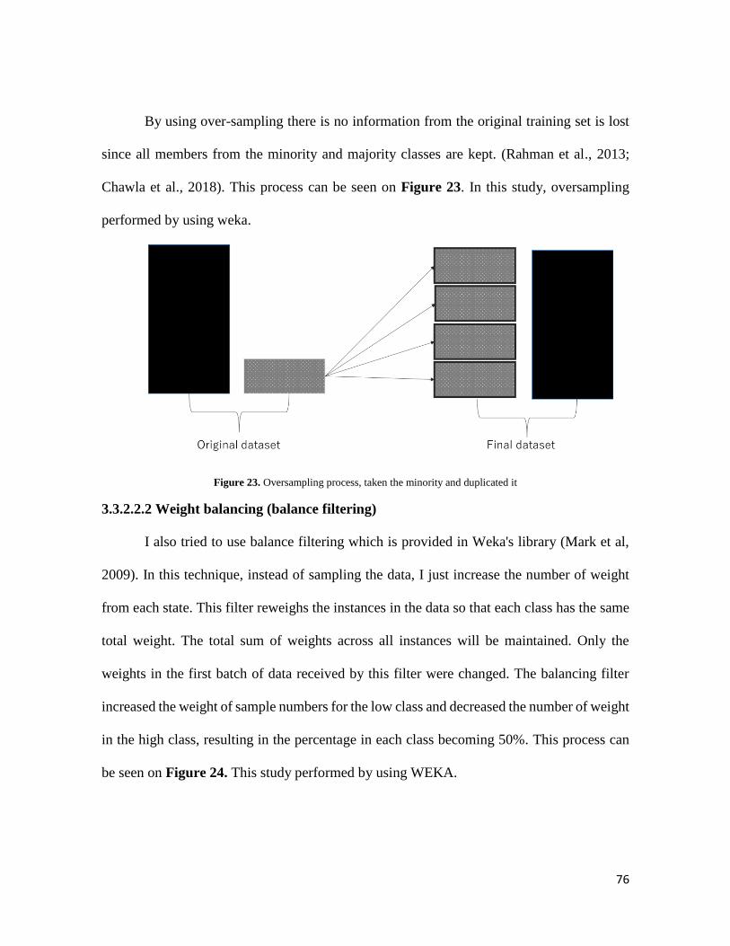
76

By using over-sampling there is no information from the original training set is lost

since all members from the minority and majority classes are kept. (Rahman et al., 2013;

Chawla et al., 2018). This process can be seen on Figure 23. In this study, oversampling

performed by using weka.

Figure 23. Oversampling process, taken the minority and duplicated it

3.3.2.2.2 Weight balancing (balance filtering)

I also tried to use balance filtering which is provided in Weka's library (Mark et al,

2009). In this technique, instead of sampling the data, I just increase the number of weight

from each state. This filter reweighs the instances in the data so that each class has the same

total weight. The total sum of weights across all instances will be maintained. Only the

weights in the first batch of data received by this filter were changed. The balancing filter

increased the weight of sample numbers for the low class and decreased the number of weight

in the high class, resulting in the percentage in each class becoming 50%. This process can

be seen on Figure 24. This study performed by using WEKA.

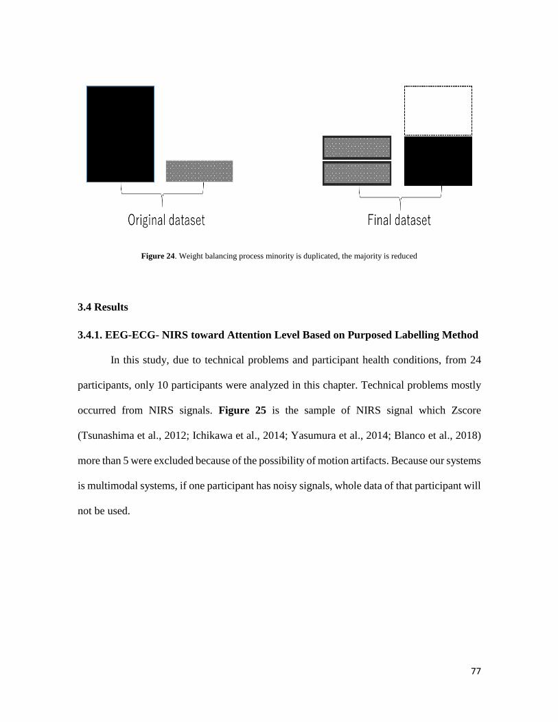
77

Figure 24. Weight balancing process minority is duplicated, the majority is reduced

3.4 Results

3.4.1. EEG-ECG- NIRS toward Attention Level Based on Purposed Labelling Method

In this study, due to technical problems and participant health conditions, from 24

participants, only 10 participants were analyzed in this chapter. Technical problems mostly

occurred from NIRS signals. Figure 25 is the sample of NIRS signal which Zscore

(Tsunashima et al., 2012; Ichikawa et al., 2014; Yasumura et al., 2014; Blanco et al., 2018)

more than 5 were excluded because of the possibility of motion artifacts. Because our systems

is multimodal systems, if one participant has noisy signals, whole data of that participant will

not be used.

78

Figure 25. Example of rejected data from NIRS

In my study, I used 59 features that were extracted from EEG, ECG, NIRS signal

which data labeling is labeled by using my proposed parameter settings from Attention level

labeling. Table 13 shows the activity of high attention and low attention toward EEG signals.

Here I calculated the average of 1800 data points from participants without balancing the

data states and applied normalization of EEG-ECG-NIRS. Normalization is applied because

I considered the differences of this multimodal signals. In this table, a Red color down arrow

shows the activity is decreased, and a green color up arrow shows the activity is increased.

From this data, we can see that relative beta is increased during high attention and relative

theta is decreased during high attention in both Fz and Pz area, on the other hand, relative

beta is decreased during low attention and relative theta is increased during low attention.

3.4.2. Classification algorithm

I adopted several classifiers to approach and investigate the best verification strategy

to evaluate recognition performance. I also investigated the best feature selector to decrease

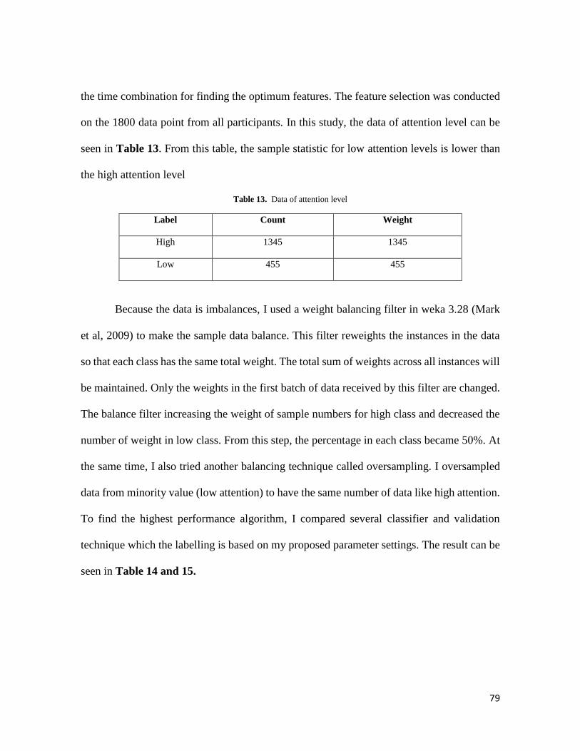
79

the time combination for finding the optimum features. The feature selection was conducted

on the 1800 data point from all participants. In this study, the data of attention level can be

seen in Table 13. From this table, the sample statistic for low attention levels is lower than

the high attention level

Table 13. Data of attention level

Label Count Weight

High 1345 1345

Low 455 455

Because the data is imbalances, I used a weight balancing filter in weka 3.28 (Mark

et al, 2009) to make the sample data balance. This filter reweights the instances in the data

so that each class has the same total weight. The total sum of weights across all instances will

be maintained. Only the weights in the first batch of data received by this filter are changed.

The balance filter increasing the weight of sample numbers for high class and decreased the

number of weight in low class. From this step, the percentage in each class became 50%. At

the same time, I also tried another balancing technique called oversampling. I oversampled

data from minority value (low attention) to have the same number of data like high attention.

To find the highest performance algorithm, I compared several classifier and validation

technique which the labelling is based on my proposed parameter settings. The result can be

seen in Table 14 and 15.

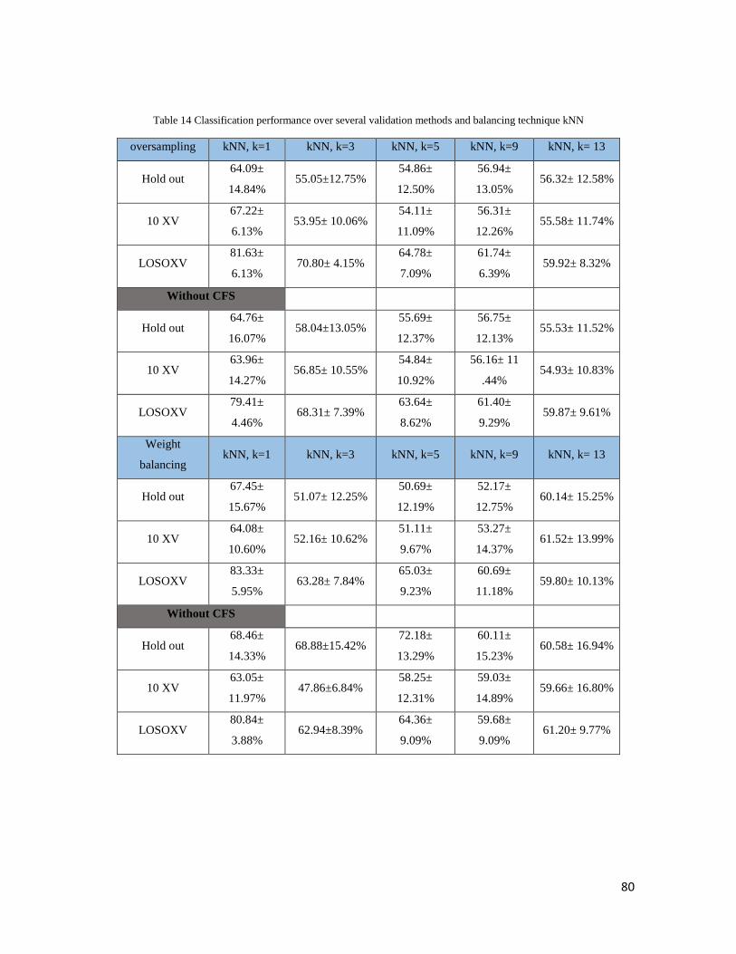
80

Table 14 Classification performance over several validation methods and balancing technique kNN

oversampling kNN, k=1 kNN, k=3 kNN, k=5 kNN, k=9 kNN, k= 13

Hold out 64.09±

14.84% 55.05±12.75%

54.86±

12.50%

56.94±

13.05% 56.32± 12.58%

10 XV 67.22±

6.13% 53.95± 10.06%

54.11±

11.09%

56.31±

12.26% 55.58± 11.74%

LOSOXV 81.63±

6.13% 70.80± 4.15%

64.78±

7.09%

61.74±

6.39% 59.92± 8.32%

Without CFS

Hold out 64.76±

16.07% 58.04±13.05%

55.69±

12.37%

56.75±

12.13% 55.53± 11.52%

10 XV 63.96±

14.27% 56.85± 10.55%

54.84±

10.92%

56.16± 11

.44% 54.93± 10.83%

LOSOXV 79.41±

4.46% 68.31± 7.39%

63.64±

8.62%

61.40±

9.29% 59.87± 9.61%

Weight

balancing kNN, k=1 kNN, k=3 kNN, k=5 kNN, k=9 kNN, k= 13

Hold out 67.45±

15.67% 51.07± 12.25%

50.69±

12.19%

52.17±

12.75% 60.14± 15.25%

10 XV 64.08±

10.60% 52.16± 10.62%

51.11±

9.67%

53.27±

14.37% 61.52± 13.99%

LOSOXV 83.33±

5.95% 63.28± 7.84%

65.03±

9.23%

60.69±

11.18% 59.80± 10.13%

Without CFS

Hold out 68.46±

14.33% 68.88±15.42%

72.18±

13.29%

60.11±

15.23% 60.58± 16.94%

10 XV 63.05±

11.97% 47.86±6.84%

58.25±

12.31%

59.03±

14.89% 59.66± 16.80%

LOSOXV 80.84±

3.88% 62.94±8.39%

64.36±

9.09%

59.68±

9.09% 61.20± 9.77%

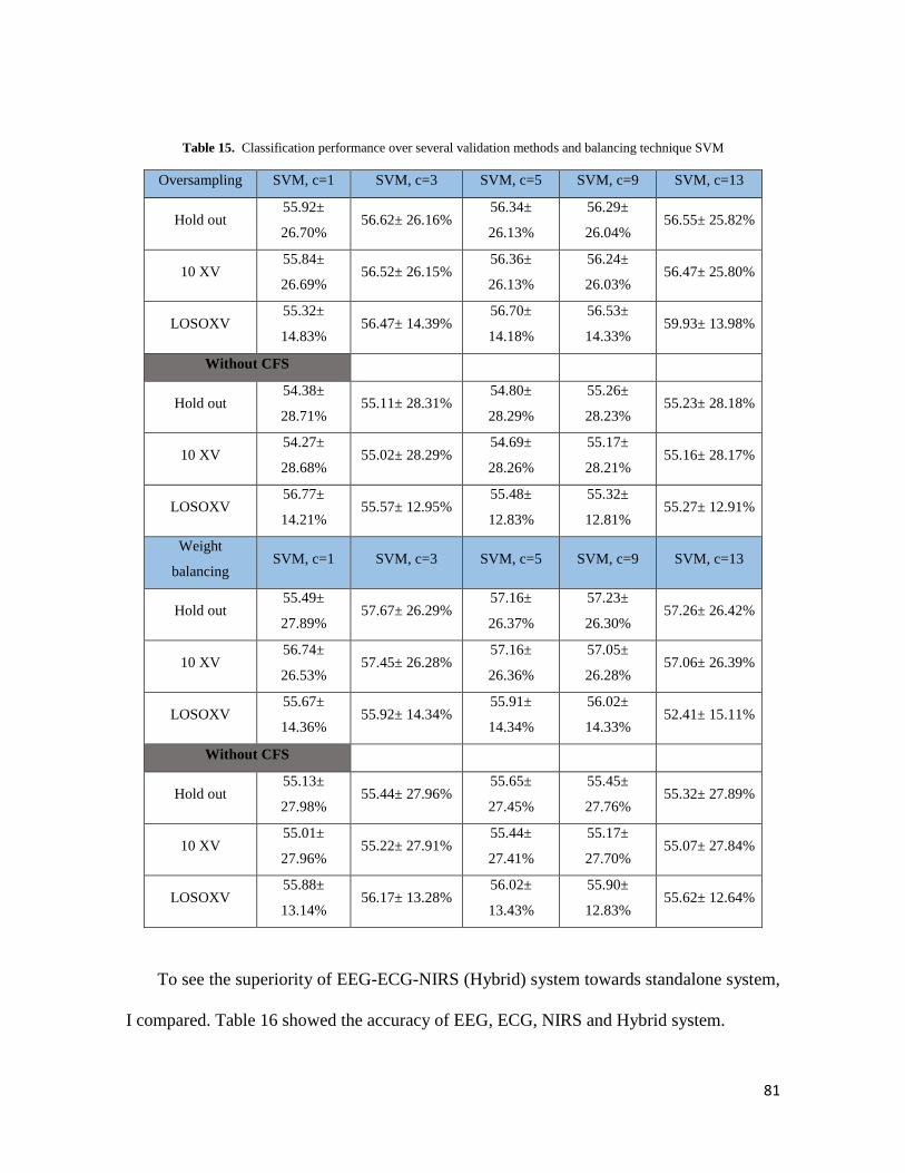
81

Table 15. Classification performance over several validation methods and balancing technique SVM

Oversampling SVM, c=1 SVM, c=3 SVM, c=5 SVM, c=9 SVM, c=13

Hold out 55.92±

26.70% 56.62± 26.16%

56.34±

26.13%

56.29±

26.04% 56.55± 25.82%

10 XV 55.84±

26.69% 56.52± 26.15%

56.36±

26.13%

56.24±

26.03% 56.47± 25.80%

LOSOXV 55.32±

14.83% 56.47± 14.39%

56.70±

14.18%

56.53±

14.33% 59.93± 13.98%

Without CFS

Hold out 54.38±

28.71% 55.11± 28.31%

54.80±

28.29%

55.26±

28.23% 55.23± 28.18%

10 XV 54.27±

28.68% 55.02± 28.29%

54.69±

28.26%

55.17±

28.21% 55.16± 28.17%

LOSOXV 56.77±

14.21% 55.57± 12.95%

55.48±

12.83%

55.32±

12.81% 55.27± 12.91%

Weight

balancing SVM, c=1 SVM, c=3 SVM, c=5 SVM, c=9 SVM, c=13

Hold out 55.49±

27.89% 57.67± 26.29%

57.16±

26.37%

57.23±

26.30% 57.26± 26.42%

10 XV 56.74±

26.53% 57.45± 26.28%

57.16±

26.36%

57.05±

26.28% 57.06± 26.39%

LOSOXV 55.67±

14.36% 55.92± 14.34%

55.91±

14.34%

56.02±

14.33% 52.41± 15.11%

Without CFS

Hold out 55.13±

27.98% 55.44± 27.96%

55.65±

27.45%

55.45±

27.76% 55.32± 27.89%

10 XV 55.01±

27.96% 55.22± 27.91%

55.44±

27.41%

55.17±

27.70% 55.07± 27.84%

LOSOXV 55.88±

13.14% 56.17± 13.28%

56.02±

13.43%

55.90±

12.83% 55.62± 12.64%

To see the superiority of EEG-ECG-NIRS (Hybrid) system towards standalone system,

I compared. Table 16 showed the accuracy of EEG, ECG, NIRS and Hybrid system.

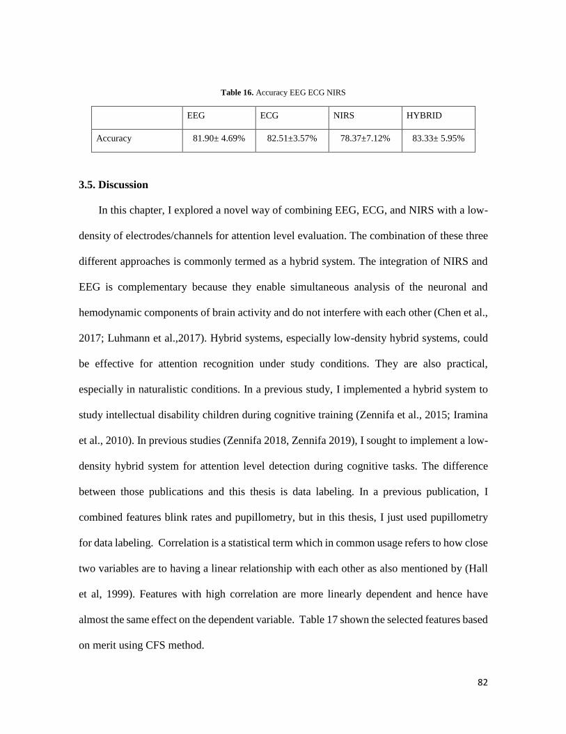
82

Table 16. Accuracy EEG ECG NIRS

EEG ECG NIRS HYBRID

Accuracy 81.90± 4.69% 82.51±3.57% 78.37±7.12% 83.33± 5.95%

3.5. Discussion

In this chapter, I explored a novel way of combining EEG, ECG, and NIRS with a low-

density of electrodes/channels for attention level evaluation. The combination of these three

different approaches is commonly termed as a hybrid system. The integration of NIRS and

EEG is complementary because they enable simultaneous analysis of the neuronal and

hemodynamic components of brain activity and do not interfere with each other (Chen et al.,

2017; Luhmann et al.,2017). Hybrid systems, especially low-density hybrid systems, could

be effective for attention recognition under study conditions. They are also practical,

especially in naturalistic conditions. In a previous study, I implemented a hybrid system to

study intellectual disability children during cognitive training (Zennifa et al., 2015; Iramina

et al., 2010). In previous studies (Zennifa 2018, Zennifa 2019), I sought to implement a low-

density hybrid system for attention level detection during cognitive tasks. The difference

between those publications and this thesis is data labeling. In a previous publication, I

combined features blink rates and pupillometry, but in this thesis, I just used pupillometry

for data labeling. Correlation is a statistical term which in common usage refers to how close

two variables are to having a linear relationship with each other as also mentioned by (Hall

et al, 1999). Features with high correlation are more linearly dependent and hence have

almost the same effect on the dependent variable. Table 17 shown the selected features based

on merit using CFS method.

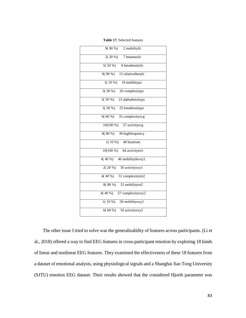
83

Table 17. Selected features

9( 90 %) 2 mobilityfz

2( 20 %) 7 betamaxfz

5( 50 %) 8 betadensityfz

9( 90 %) 15 relativethetafz

1( 10 %) 19 mobilitypz

3( 30 %) 20 complexitypz

5( 50 %) 23 alphadensitypz

3( 30 %) 25 betadensitypz

6( 60 %) 35 complexityecg

10(100 %) 37 activityecg

8( 80 %) 39 highfrequency

1( 10 %) 40 heartrate

10(100 %) 44 activitytot1

4( 40 %) 46 mobilitydeoxy1

2( 20 %) 50 activityoxy1

4( 40 %) 51 complexitytot2

8( 80 %) 52 mobilitytot2

4( 40 %) 57 complexityoxy2

1( 10 %) 58 mobilityoxy2

6( 60 %) 59 activityoxy2

The other issue I tried to solve was the generalizability of features across participants. (Li et

al., 2018) offered a way to find EEG features in cross-participant emotion by exploring 18 kinds

of linear and nonlinear EEG features. They examined the effectiveness of these 18 features from

a dataset of emotional analysis, using physiological signals and a Shanghai Jiao Tong University

(SJTU) emotion EEG dataset. Their results showed that the considered Hjorth parameter was

84

suitable for analyzing EEG signals. In their evaluation, they found the Hjorth parameter in the

beta rhythm led to the best mean recognition accuracy in cross-subject emotion recognition. In

our study, we used nine types of linear and nonlinear features to find the most common feature

to be used in attention recognition. As shown in Table 17, some Hjorth parameter was selected

as a feature by CFS + kNN. (Oh et al., 2014) applied the Hjorth parameter for extracting EEG

features. They found that the Hjorth parameter increased their EEG classification by 4.4%, on

average. Following that, I suggest that the Hjorth parameter could be a useful feature for EEG-

ECG- NIRS in attention recognition. After doing feature extraction I calculated predictive

modeling by using several classifiers. kNN with k=1 was selected in this system after we

compared it with other kernels and another classifier. Accuracy performance is higher in k=1

could be happened because the data is binary data, I also investigated other classifier

performance for example SVM (55.88± 13.14%) (poly kernel), but the accuracy performance

that I got is lower kNN (80.84± 3.88%). kNN classifier also mentioned in the study (Ahn et

al., 2010) has the highest accuracy among another classifier especially when combine with

CFS feature selector. In their study, they got the result of the kNN classifier. KNN has better

accuracy than SVM, it’s also mentioned in (Palaniappan et al, 2014) which this result also

has been shown in my study.

3.6. Conclusions

This study sought to investigate the usability of a low-density hybrid system in

attention recognition. My result showed the accuracy system of low-density EEG-ECG-

NIRS (83.33± 5.95%) has the highest accuracy compare with EEG (81.90± 4.69%), ECG

(82.51±3.57%), NIRS (78.37±7.12%). CFS+kNN algorithm also showed highest

85

performance compare with other methods such as CFS+SVM (55.49± 27.89%), kNN

(80.84± 3.88%) and SVM (55.88± 13.14%).

86

Chapter 4. General Discussion

I have proposed a parameter settings for data labeling in attention level detection and

applied this labeling method to low-density EEG-ECG-NIRS. Several studies have proposed

labeling methods such as self-assessment, observation, objective performance for detecting

attention level. The system proposed in this thesis is specific parameter settings as the new

labeling method for attention recognition using eye information and apply it in EEG-ECG-

NIRS low density. Several research in multimodal systems required many channels (Ahn et

al., 2017; Punsawad et al., 2017; Huang et al., 2018). But this thesis tried to use multimodal

systems in few channels.

In chapter 2, I talked about the difference evaluation between self-assessment and the

effect of attention level toward blink rates and pupillometry. Self-assessment has been

compared for checking the similarity of this self-assessments method compared other

methods such as observation and objective performance. Later on, self-assessment used as

validation data in parameter setting using pupillometry to evaluate the difference evaluation.

I found that error rates and difference evaluation of those systems comparing self-assessment

is less than 21%. From chapter 2, I concluded that data from self-assessment can be the basis

for developing our quantitative algorithm for new labeling method in attention level detection.

Further analysis, I found that blink rates during high attention are lower than low attention in

my cognitive task experiment. Pupillometry during high attention is bigger than low attention.

Generally, between each blink is an interval of 2–10 seconds; actual rates vary by

individual averaging around 10 blinks per minute in a laboratory setting. However, when the

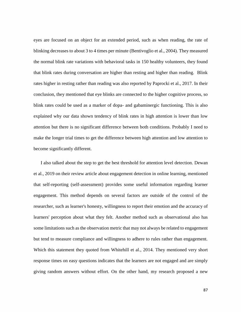
87

eyes are focused on an object for an extended period, such as when reading, the rate of

blinking decreases to about 3 to 4 times per minute (Bentivoglio et al., 2004). They measured

the normal blink rate variations with behavioral tasks in 150 healthy volunteers, they found

that blink rates during conversation are higher than resting and higher than reading. Blink

rates higher in resting rather than reading was also reported by Paprocki et al., 2017. In their

conclusion, they mentioned that eye blinks are connected to the higher cognitive process, so

blink rates could be used as a marker of dopa- and gabaminergic functioning. This is also

explained why our data shown tendency of blink rates in high attention is lower than low

attention but there is no significant difference between both conditions. Probably I need to

make the longer trial times to get the difference between high attention and low attention to

become significantly different.

I also talked about the step to get the best threshold for attention level detection. Dewan

et al., 2019 on their review article about engagement detection in online learning, mentioned

that self-reporting (self-assessment) provides some useful information regarding learner

engagement. This method depends on several factors are outside of the control of the

researcher, such as learner's honesty, willingness to report their emotion and the accuracy of

learners' perception about what they felt. Another method such as observational also has

some limitations such as the observation metric that may not always be related to engagement

but tend to measure compliance and willingness to adhere to rules rather than engagement.

Which this statement they quoted from Whitehill et al., 2014. They mentioned very short

response times on easy questions indicates that the learners are not engaged and are simply

giving random answers without effort. On the other hand, my research proposed a new

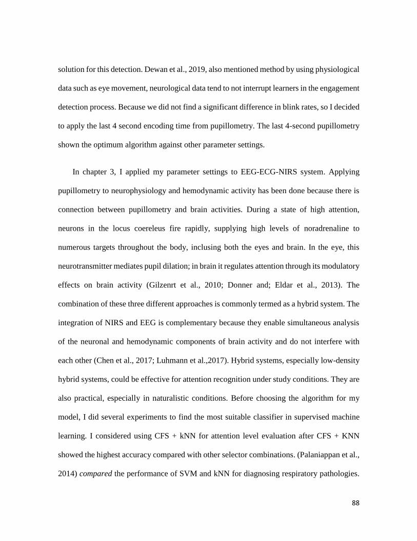
88

solution for this detection. Dewan et al., 2019, also mentioned method by using physiological

data such as eye movement, neurological data tend to not interrupt learners in the engagement

detection process. Because we did not find a significant difference in blink rates, so I decided

to apply the last 4 second encoding time from pupillometry. The last 4-second pupillometry

shown the optimum algorithm against other parameter settings.

In chapter 3, I applied my parameter settings to EEG-ECG-NIRS system. Applying

pupillometry to neurophysiology and hemodynamic activity has been done because there is

connection between pupillometry and brain activities. During a state of high attention,

neurons in the locus coereleus fire rapidly, supplying high levels of noradrenaline to

numerous targets throughout the body, inclusing both the eyes and brain. In the eye, this

neurotransmitter mediates pupil dilation; in brain it regulates attention through its modulatory

effects on brain activity (Gilzenrt et al., 2010; Donner and; Eldar et al., 2013). The

combination of these three different approaches is commonly termed as a hybrid system. The

integration of NIRS and EEG is complementary because they enable simultaneous analysis

of the neuronal and hemodynamic components of brain activity and do not interfere with

each other (Chen et al., 2017; Luhmann et al.,2017). Hybrid systems, especially low-density

hybrid systems, could be effective for attention recognition under study conditions. They are

also practical, especially in naturalistic conditions. Before choosing the algorithm for my

model, I did several experiments to find the most suitable classifier in supervised machine

learning. I considered using CFS + kNN for attention level evaluation after CFS + KNN

showed the highest accuracy compared with other selector combinations. (Palaniappan et al.,

2014) compared the performance of SVM and kNN for diagnosing respiratory pathologies.

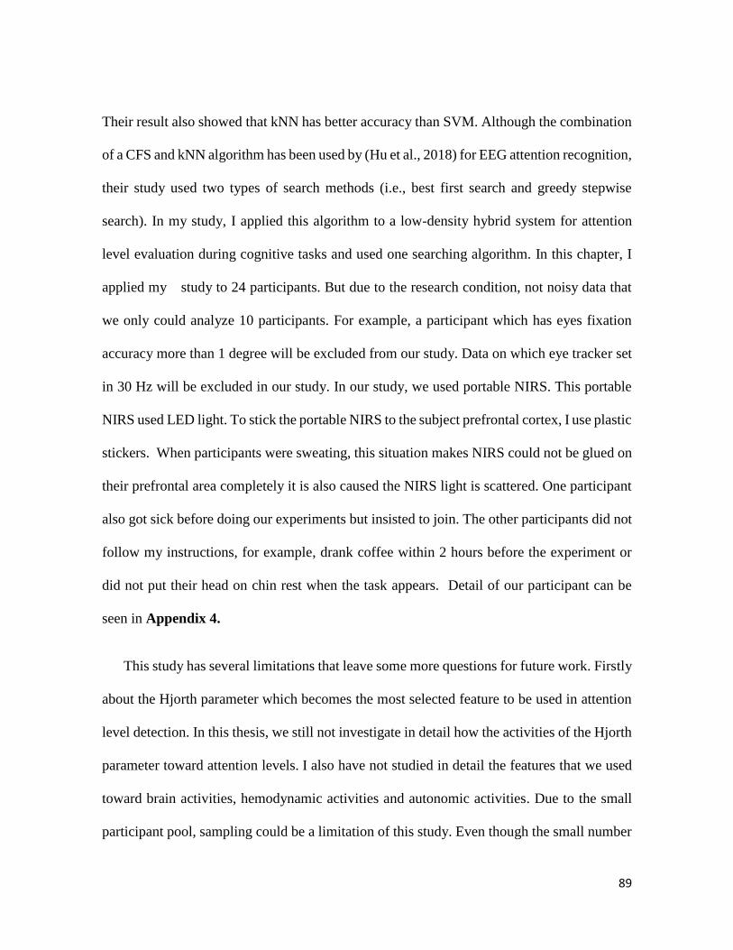
89

Their result also showed that kNN has better accuracy than SVM. Although the combination

of a CFS and kNN algorithm has been used by (Hu et al., 2018) for EEG attention recognition,

their study used two types of search methods (i.e., best first search and greedy stepwise

search). In my study, I applied this algorithm to a low-density hybrid system for attention

level evaluation during cognitive tasks and used one searching algorithm. In this chapter, I

applied my study to 24 participants. But due to the research condition, not noisy data that

we only could analyze 10 participants. For example, a participant which has eyes fixation

accuracy more than 1 degree will be excluded from our study. Data on which eye tracker set

in 30 Hz will be excluded in our study. In our study, we used portable NIRS. This portable

NIRS used LED light. To stick the portable NIRS to the subject prefrontal cortex, I use plastic

stickers. When participants were sweating, this situation makes NIRS could not be glued on

their prefrontal area completely it is also caused the NIRS light is scattered. One participant

also got sick before doing our experiments but insisted to join. The other participants did not

follow my instructions, for example, drank coffee within 2 hours before the experiment or

did not put their head on chin rest when the task appears. Detail of our participant can be

seen in Appendix 4.

This study has several limitations that leave some more questions for future work. Firstly

about the Hjorth parameter which becomes the most selected feature to be used in attention

level detection. In this thesis, we still not investigate in detail how the activities of the Hjorth

parameter toward attention levels. I also have not studied in detail the features that we used

toward brain activities, hemodynamic activities and autonomic activities. Due to the small

participant pool, sampling could be a limitation of this study. Even though the small number

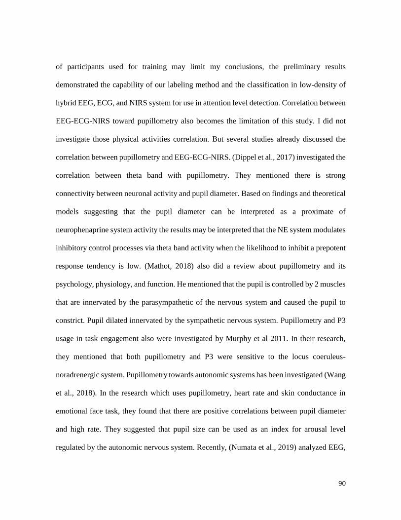
90

of participants used for training may limit my conclusions, the preliminary results

demonstrated the capability of our labeling method and the classification in low-density of

hybrid EEG, ECG, and NIRS system for use in attention level detection. Correlation between

EEG-ECG-NIRS toward pupillometry also becomes the limitation of this study. I did not

investigate those physical activities correlation. But several studies already discussed the

correlation between pupillometry and EEG-ECG-NIRS. (Dippel et al., 2017) investigated the

correlation between theta band with pupillometry. They mentioned there is strong

connectivity between neuronal activity and pupil diameter. Based on findings and theoretical

models suggesting that the pupil diameter can be interpreted as a proximate of

neurophenaprine system activity the results may be interpreted that the NE system modulates

inhibitory control processes via theta band activity when the likelihood to inhibit a prepotent

response tendency is low. (Mathot, 2018) also did a review about pupillometry and its

psychology, physiology, and function. He mentioned that the pupil is controlled by 2 muscles

that are innervated by the parasympathetic of the nervous system and caused the pupil to

constrict. Pupil dilated innervated by the sympathetic nervous system. Pupillometry and P3

usage in task engagement also were investigated by Murphy et al 2011. In their research,

they mentioned that both pupillometry and P3 were sensitive to the locus coeruleus-

noradrenergic system. Pupillometry towards autonomic systems has been investigated (Wang

et al., 2018). In the research which uses pupillometry, heart rate and skin conductance in

emotional face task, they found that there are positive correlations between pupil diameter

and high rate. They suggested that pupil size can be used as an index for arousal level

regulated by the autonomic nervous system. Recently, (Numata et al., 2019) analyzed EEG,

91

NIRS and pupil diameter toward attention during a free recall task. They found that there are

significant physiological responses among those 3 modals. They recommend considering the

characteristic of these multimodal in the development of applications requiring attention.

Overall, these results demonstrated that the proposed method can be used to be data

labeling for other physiological signals such as electroencephalograph (EEG),

electrocardiograph (ECG), and near-infrared spectroscopy (NIRS). After that, this parameter

settings was applied to EEG-ECG-NIRS for attention level detection. Two-electrode wireless

EEG, a wireless ECG, and two wireless channels NIRS has been used to detect attention

levels during cognitive tasks. Algorithm CFS+kNN also shown highest performance

compare with other methods such as CFS+SVM (55.49± 27.89%), kNN (80.84± 3.88%) and

SVM (55.88± 13.14%). On the same time, I found that my result showed the accuracy system

of EEG-ECG-NIRS (83.33± 5.95%) has the highest accuracy compare with EEG (81.90±

4.69%), ECG (82.51±3.57%), NIRS (78.37±7.12%).

92

Acknowledgement “if you think you will fail, you will be really failed. No one will trust you except yourself.

If you doubt yourself who will trust you”. This is my mantra when I would like to give up on

anything.

I came to Japan in autumn 2013, after I finished my study in undergraduate with theme

artificial intelligence to detect cardiovascular disease. My master study, entitled the change

of EEG, ECG, and NIRS in Mental retardation child during four education training give me

a new insight into brain sciences and developmental disorder. The next years after I

completed my master thesis, I am thinking to develop a system by using hybrid systems. I

was aspiring to be the youngest doctor from Indonesia in systems life sciences. But quarter

life crisis was hit me and unfortunately, I should extend my studies. That moment was the

bitterest experience in my life. But thanks to everyone who tries to convince me that life is

not about age, but contribution. Finally, I finished my study in 2020, where Corona virus

become a big terror in human existence.

On this page, I would like to show my greatest appreciation to Prof. Iramina who offered

continuing support and constant encouragement. Thanks to Prof. Lauwereyns , Prof.

Okamoto, and Prof. Morooka, who gave me advice for my research. I would like to thank to

all my new families in Japan who support my studies in Japan. When I was in Maidashi

campus, almost every day the staff or the driver said “ganbatte” to me. Thanks to Indonesian

student association in Japan, I got experience about leadership through this organization.

Thanks to Systems Life sciences office, International Office support center Kyushu

University, who always helps to process my documents. Special to Dr. Alexandra Wolf a.k.a

Ola, Sho Ageno, Nonthaporn Nakphu, Chi Tran, Reza, thank you very much for support me

in academic or in personal life. For Shirouzu Makoto sensei, thank you very much for guiding

me to find the peace in my mind. Prof. Alexander Staykov who gave me the first part time

job in Japan. I also would like to say my great thank to Damanhuri Family that always support

my study in Japan. Of course to my parents, Zen and Dr. Hanifah who always try to calm me

down when I feel so stress during study.

The last, I would like to say thank you to Asahi Glass Company Scholarship foundation,

Otsuka Toshimi Foundation, Kyushu Doctoral Scholarship who support my study in Japan.

93

References

Aghajani H, Garbey M and Omurtag A (2017) Measuring Mental Workload with

EEG+fNIRS. Front. Hum. Neurosci. 11:359. doi: 10.3389/fnhum.2017.00359

Ahn, S., Nguyen, T., Jang, H., Kim, J. G., & Jun, S. C. (2016). Exploring Neuro-

Physiological Correlates of Drivers' Mental Fatigue Caused by Sleep Deprivation Using

Simultaneous EEG, ECG, and fNIRS Data. Frontiers in human neuroscience, 10, 219.

doi:10.3389/fnhum.2016.00219

Ahn S and Jun SC (2017) Multi-Modal Integration of EEG-fNIRS for Brain-Computer

Interfaces – Current Limitations and Future Directions. Front. Hum. Neurosci. 11:503.

doi: 10.3389/fnhum.2017.00503

Altman, N. S. (1992). "An introduction to kernel and nearest-neighbor nonparametric

regression" (PDF). The American Statistician. 46 (3): 175–185.

doi:10.1080/00031305.1992.10475879. hdl:1813/31637.

Anderson, John R. (2004). Cognitive psychology and its implications (6th ed.), Worth

Publishers.

Benedetto, S., Carbone, A., Drai-Zerbib, V., Pedrotti, M., & Baccino, T. (2014.). Effects of

luminance and illuminance on visual fatigue and arousal during digital reading.

Computers in Human Behavior, 41, 112-119.http://dx.doi.org/10.1016/j.chb.2014.09.023

Bentivoglio, A. R.; Bressman, S. B.; Cassetta, E.; Carretta, D.; Tonali, P.; Albanese, A.

(November 1997). "Analysis of blink rate patterns in normal subjects". Movement

Disorders. 12 (6): 1028–1034. doi:10.1002/mds.870120629. ISSN 0885-3185. PMID

9399231.

94

Berka, C., Levendowski, D. J., Lumicao, M. N., Yau, A., Davis, G., Zivkovic, V. T., …

Craven, P. L. (2007). EEG Correlates of Task Engagement and Mental Workload in

Vigilance, Learning, and Memory Tasks.

Blanco Borja, Monika Molnar, and César Caballero-Gaudes "Effect of prewhitening in

resting-state functional near-infrared spectroscopy data," Neurophotonics 5(4), 040401

(24 October 2018). https://doi.org/10.1117/1.NPh.5.4.040401

Börger, N., Van Der Meere, J., Ronner, A., Alberts, E., Geuze, R., & Bogte, H. (1999). Heart

rate variability and sustained attention in ADHD children. Journal of Abnormal Child

Psychology, 27(1), 25–33. https://doi.org/10.1023/A:1022610306984

Bulling, A., Ward, J. A., Gellersen, H., & Oster, G. T. (2011). Eye Movement Analysis for

Activity Recognition Using Electrooculography. IEEE Trans. Pattern Anal. Mach. Intell.

2011, 33, 741–753, doi:10.1109/TPAMI.2010.86.

H. Burton, N.S. Abend, A.-M.K. MacLeod, R.J. Sinclair, A.Z. Snyder, M.E. Raichle, Tactile

Attention Tasks Enhance Activation in Somatosensory Regions of Parietal Cortex: A

Positron Emission Tomography Study, Cerebral Cortex, Volume 9, Issue 7, October 1999,

Pages 662–674,

Campbell, A. M., & Davalos, D. B. (2015). Levels of attention and task difficulty in the

modulation of interval duration mismatch negativity. Frontiers in Psychology,

6(OCT), 1–7. https://doi.org/10.3389/fpsyg.2015.01619

Chandra S, Sharma G, Sharma M, Jha D, Mittal AP. Workload regulation by Sudarshan

Kriya: an EEG and ECG perspective. Brain Inform. 2017 Mar;4(1):13-25. doi:

10.1007/s40708-016-0055-1. Epub 2016 Jul 18.

95

Chang, Y. C., & Huang, S. L. (2012). The influence of attention levels on

psychophysiological responses. International Journal of Psychophysiology.

https://doi.org/10.1016/j.ijpsycho.2012.09.001

Chayer, C.; Freedman, M. (2001). Frontal lobe functions. Curr. Neurol. Neurosci. Rep. 2001,

1, 547–552.

Chawla, Nitesh V.; Herrera, Francisco; Garcia, Salvador; Fernandez, Alberto (2018-04-20).

"SMOTE for Learning from Imbalanced Data: Progress and Challenges, Marking the 15-

year Anniversary". Journal of Artificial Intelligence Research. 61: 863–905.

doi:10.1613/jair.1.11192. ISSN 1076-9757

Chen, C.-W.; Sun, C.-W. (2017) Combination of Electroencephalography and Near-Infrared

Spectroscopy in Evaluation of Mental Concentration during the Mental Focus Task for

Wisconsin Card Sorting Test. Sci. Rep.2017, 7, 338.

Chicco, D. (2017). Ten quick tips for machine learning in computational biology. BioData

Min. 2017, 10, 35.

Corral-López, A., Garate-Olaizola, M., Buechel, S. D., Kolm, N., & Kotrschal, A. (2017).

On the role of body size, brain size, and eye size in visual acuity. Behavioral ecology and

sociobiology, 71(12), 179. doi:10.1007/s00265-017-2408-z

Cortes, Corinna; Vapnik, Vladimir N. (1995). Support-vector networks. Machine Learning.

20 (3): 273–297. CiteSeerX 10.1.1.15.9362. doi:10.1007/BF00994018.

Culham, J.C.; Valyear, K.F. (2006). Human parietal cortex in action. Curr. Opin. Neurobiol.

2006, 16, 205–212.


96

Cullum, C. M. (1998). Neuropsychological Assessment of Adults. In Neuropsychology (pp.

357–378). https://doi.org/10.1007/978-1-4899-1950-2_17

Dalmaijer, E. S. (n.d.). Is the low-cost EyeTribe eye tracker any good for research?

https://doi.org/10.7287/peerj.preprints.585v1

De Oliveira, R.A.M.; Araújo, L.F.; De Figueiredo, R.C.; Goulart, A.C.; Schmidt, M.I.;

Barreto, S.M.; Ribeiro, A.L.P. (2017). Coffee Consumption and Heart Rate Variability:

The Brazilian Longitudinal Study of Adult Health (ELSA-Brasil) Cohort

Study. Nutrients 2017, 9, 741.

Dewan, M. A. A., Murshed, M., & Lin, F. (2019). Engagement detection in online learning:

a review. Smart Learning Environments, 6(1), 1–20. https://doi.org/10.1186/s40561-018-

0080-z

Derosière G, Mandrick K, Dray G, Ward TE and Perrey S (2013) NIRS-measured prefrontal

cortex activity in neuroergonomics: strengths and weaknesses. Front. Hum. Neurosci.

7:583. doi: 10.3389/fnhum.2013.00583

Donner,T.H.,andNieuwenhuis,S.(2013).Brain-widegainmodulation:therich get richer.

Nat.Neurosci. 16, 989–990.doi:10.1038/nn.3471

Dippel, G., Mückschel, M., Ziemssen, T., & Beste, C. (2017). Demands on response

inhibition processes determine modulations of theta band activity in superior frontal

areas and correlations with pupillometry – Implications for the norepinephrine system

during inhibitory control. NeuroImage.

https://doi.org/10.1016/j.neuroimage.2017.06.037

https://doi.org/10.7287/peerj.preprints.585v1

https://doi.org/10.1186/s40561-018-0080-z

https://doi.org/10.1186/s40561-018-0080-z

https://doi.org/10.1016/j.neuroimage.2017.06.037

97

Donders FC (1969) On the speed of mental processes. Acta Psychol 30: 412–431.

[Translation of: Die Schnelligkeit psychischer Processe, first published in 1868].

D.Y. Fougnie. (2008).The relationship between attention and working memory. N.B.

Johansen (Ed.), New research on short-term memory, Nova Science Publishers,

Hauppage (2008), pp. 1-45

Eldar,E.,Cohen,J.D.,andNiv,Y.(2013).Theeffectsofneuralgainonattention and learning.

Nat.Neurosci. 16, 1146–1153.doi:10.1038/nn.3428

Franco, A., Neves, C. M., Quintão, C., Vigário, R., & Vieira, P. (2014). Singular Spectrum

Analysis of Pupillometry Data. Identification of the Sympathetic and Parasympathetic

Activity. Procedia Technology, 17, 273–280.

https://doi.org/10.1016/j.protcy.2014.10.237

Geva, R., Zivan, M., Warsha, A., & Olchik, D. (2013). Alerting, orienting or executive

attention networks: Differential patters of pupil dilations. Frontiers in Behavioral

Neuroscience, 7, 145.

Gholami, B., Bailey, J. M., Haddad, W. M., & Tannenbaum, A. R. (2012). Clinical decision

support and closed-loop control for cardiopulmonary management and intensive care

unit sedation using expert systems. IEEE Transactions on Control Systems Technology,

20(5), 1343–1350. https://doi.org/10.1109/TCST.2011.2162412

Gilzenrat,M.S.,Nieuwenhuis,S.,Jepma,M.,andCohen,J.D.(2010).Pupil diameter tracks

changes in control state predicted by the adaptive gain theory of locus coeruleus function.

Cogn.Affect.Behav.Neurosci. 10, 252–269.doi:10.3758/CABN.10.2.252

https://doi.org/10.1016/j.protcy.2014.10.237

https://doi.org/10.1109/TCST.2011.2162412

98

Griffiths, K. R., Quintana, D. S., Hermens, D. F., Spooner, C., Tsang, T. W., Clarke, S., &

Kohn, M. R. (2017). Sustained attention and heart rate variability in children and

adolescents with ADHD. Biological Psychology, 124, 11–20.

https://doi.org/10.1016/j.biopsycho.2017.01.004

Granholm E, Steinhauer SR. Pupillometric measures of cognitive and emotional processes.

Int J Psychophysiol. 2004 Mar;52(1): 1-6.DOI: 10.1016/j.ijpsycho.2003.12.001

Hall M., Frank E., Holmes G., Pfahringer B., Reutemann P., Witten I.H. (2009). The WEKA

data mining software: An update. SIGKDD Explor. doi: 10.1145/1656274.1656278

Hall M. Ph.D. Thesis. Waikato University; Hamilton, New Zealand: 1999. Correlation-Based

Feature Selection for Machine Learning.

Hartmann, M., & Fischer, M. H. (2014). Pupillometry: The eyes shed fresh light on the mind.

Current Biology, 24(7), R281–R282. https://doi.org/10.1016/j.cub.2014.02.028

He S, Li Y. (2017). A Single-Channel EOG-Based Speller. IEEE Trans Neural Syst Rehabil

Eng. 2017 Nov;25(11):1978-1987. doi: 10.1109/TNSRE.2017.2716109. Epub 2017 Jun

15.

Hong K-S, Khan MJ and Hong MJ (2018) Feature Extraction and Classification Methods for

Hybrid fNIRS-EEG Brain-Computer Interfaces. Front. Hum. Neurosci. 12:246. doi:

10.3389/fnhum.2018.00246

Hoang T. et al. (2012) Time Domain Parameters for Online Feedback fNIRS-Based Brain-

Computer Interface Systems. In: Huang T., Zeng Z., Li C., Leung C.S. (eds) Neural

Information Processing. ICONIP 2012. Lecture Notes in Computer Science, vol 7664.

Springer, Berlin, Heidelberg

https://doi.org/10.1016/j.cub.2014.02.028

99

Hu, B.; Li, X.; Sun, S.; Ratcliffe, M. (2018). Attention Recognition in EEG-Based Affective

Learning Research Using CFS+KNN Algorithm. IEEE/ACM Trans. Comput. Biol;

Bioinform. 2018, 15, 38–45

Huang, S.; Li, J.; Zhang, P.; Zhang, W. (2018). Detection of mental fatigue state with

wearable ECG devices. Int. J. Med. Inform. 2018, 119, 39–46.

Huang Q, He S, Wang Q, Gu Z, Peng N, Li K, Zhang Y, Shao M, Li Y. An EOG-Based

Human-Machine Interface for Wheelchair Control. IEEE Trans Biomed Eng. 2018

Sep;65(9):2023-2032. doi: 10.1109/TBME.2017.2732479. Epub 2017 Jul 27.

Ichikawa H, Kitazono J, Nagata K, Manda A, Shimamura K, Sakuta R, Okada M, Yamaguchi

MK, Kanazawa S and Kakigi R (2014) Novel method to classify hemodynamic response

obtained using multi-channel fNIRS measurements into two groups: exploring the

combinations of channels. Front. Hum. Neurosci. 8:480. doi: 10.3389/fnhum.2014.00480

Iramina K., Matsuda K., Ide J., Noguchi Y. (2010).Monitoring system of neuronal activity

and moving activity without restraint using wireless EEG, NIRS and accelerometer;

Proceedings of the 2010 IEEE EMBS Conference on Biomedical Engineering and

Sciences, IECBES; Kuala Lumpur, Malaysia. 30 November–2 December 2010; pp. 481–

484

James, W. (1890). The Principles of Psychology, in two volumes. New York: Henry Holt

and Company.

Jensen, A. R., & Figueroa, R. A. (1975). Forward and backward digit span interaction with

race and IQ: Predictions from Jensen's theory [abstract]. Journal of Educational

Psychology, 67(6), 882-893.

100

Johnson, E. L., Miller Singley, A. T., Peckham, A. D., Johnson, S. L., & Bunge, S. A.

(2014). Task-evoked pupillometry provides a window into the development of short-

term memory capacity. Frontiers in Psychology, 5(MAR), 1–8.

https://doi.org/10.3389/fpsyg.2014.00218

Joshi, S., Li, Y., Kalwani, R. M., & Gold, J. I. (2016). Relationships between Pupil Diameter

and Neuronal Activity in the Locus Coeruleus, Colliculi, and Cingulate Cortex. Neuron,

89(1). https://doi.org/10.1016/j.neuron.2015.11.028

Kaneko H, Yoshikawa T, Nomura K, Ito H, Yamauchi H, Ogura M, Honjo S. Hemodynamic

changes in the prefrontal cortex during digit span task: a near-infrared spectroscopy study.

Neuropsychobiology. 2011;63(2):59-65. doi: 10.1159/000323446. Epub 2010 Dec 20.

Kang, O. E., Huffer, K. E., & Wheatley, T. P. (2014). Pupil Dilation Dynamics Track

Attention to High-Level Information. PLoS ONE, 9(8), 102463.

https://doi.org/10.1371/journal

Karatekin, C. (2004). Development of attentional allocation in the dual task paradigm.

International Journal of Psychophysiology, 52, 7–21.

Karatekin, C., Marcus, D. J., & Couperus, J. W. (2007). Regulation of cognitive resources

during sustained attention and working memory in 10-year-olds and adults.

Psychophysiology, 44, 128–144.

Koenig S., Uengoer M., Lachnit H. (2017) Pupil dilation indicates the coding of past

prediction errors: Evidence for attentional learning theory. Psychophysiology 55(4):

e13020 doi:10.1111/psyp.13020

https://doi.org/10.1016/j.neuron.2015.11.028

https://doi.org/10.1371/journal

101

Koichubekov, B., Korshukov, I., Omarbekova, N., Riklefs, V., Sorokina, M., & Mkhitaryan,

X. (2015). Computation of nonlinear parameters of heart rhythm using short time ECG

segments. Computational and mathematical methods in medicine, 2015, 983479.

doi:10.1155/2015/983479

Kolmogorov AN. 1965. Three approaches to the quantitative definition of information.

Problemsof Information and Transmission 1(1):1–7

Langner R, Eickhoff SB. Sustaining attention to simple tasks: a meta-analytic review of the

neural mechanisms of vigilant attention. Psychol Bull. 2013 Jul; 139(4):870-900. doi:

10.1037/a0030694. Epub 2012 Nov 19.

Li X, Song D, Zhang P, Zhang Y, Hou Y and Hu B (2018) Exploring EEG Features in Cross-

Subject Emotion Recognition. Front. Neurosci. 12:162. doi: 10.3389/fnins.2018.00162

Lilly, Leonard S, ed. (2016). Pathophysiology of Heart Disease: A Collaborative Project of

Medical Students and Faculty (sixth ed.). Lippincott Williams & Wilkins. p. 74. ISBN

978-1451192759.

Liu, N. H., Chiang, C. Y., & Chu, H. C. (2013). Recognizing the degree of human attention

using EEG signals from mobile sensors. Sensors (Basel, Switzerland), 13(8), 10273–

10286. doi:10.3390/s130810273

Luhmann, V.A.; Muller, K.R. (2017). Why build an integrated EEG-NIRS? About the

advantages of hybrid bio-acquisition hardware. IEEE Eng. Med. Biol. Soc. 2017, 4475–

4478.

102

Lui, L. T., Terrazas, G., Zenil, H., Alexander, C., & Krasnogor, N. (2015). Complexity

measurement based on information theory and Kolmogorov complexity. Artificial Life.

https://doi.org/10.1162/ARTL_a_00157

Marc Argilés, Genís Cardona, Elisabet Pérez-Cabré, Margarita Rodríguez; Blink Rate and

Incomplete Blinks in Six Different Controlled Hard-Copy and Electronic Reading

Conditions. Invest. Ophthalmol. Vis. Sci. 2015;56(11):6679-6685. doi: 10.1167/iovs.15-

16967.

Martínez-Sellés, M., Datino, T., Figueiras-Graillet, L. et al. Clinical Drug Investigation

(2013) 33: 45. https://doi.org/10.1007/s40261-012-0032-2

Mathôt, S. 2018 Pupillometry: Psychology, Physiology, and Function. Journal of Cognition,

1(1): 16, pp. 1–23, DOI: https://doi.org/10.5334/joc.18

Matsuda, G., & Hiraki, K. (2006). Sustained decrease in oxygenated hemoglobin during

video games in the dorsal prefrontal cortex: A NIRS study of children. NeuroImage, 29(3),

706–711. https://doi.org/10.1016/j.neuroimage.2005.08.019

Müller JA, Wendt D, Kollmeier B, Brand T (2016) Comparing Eye Tracking with

Electrooculography for Measuring Individual Sentence Comprehension Duration. PLOS

ONE 11(10): e0164627. https://doi.org/10.1371/journal.pone.0164627

Murphy PR, Robertson IH, Balsters JH, O'connell RG. 2011. Pupillometry and P3 index the

locus coeruleus-noradrenergic arousal function in humans. Psychophysiology. 2011

Nov;48(11):1532-1543. doi: 10.1111/j.1469-8986.2011.01226.x. Epub 2011 Jul 18.

Naber, M., Alvarez, G.A., and Nakayama, K. (2013). Tracking the allocation of attention

using human pupillary oscillations. Front.Psychol. 4, 919.

https://doi.org/10.1007/s40261-012-0032-2

https://doi.org/10.5334/joc.18

https://doi.org/10.1371/journal.pone.0164627

103

Nakano, T., Kato, M., Morito, Y., Itoi, S., & Kitazawa, S. (2013). Blink-related momentary

activation of the default mode network while viewing videos. Proceedings of the National

Academy of Sciences of the United States of America, 110(2), 702–706.

doi:10.1073/pnas.1214804110

Numata T, Kiguchi M and Sato H (2019) Multiple-Time-Scale Analysis of Attention as

Revealed by EEG, NIRS, and Pupil Diameter Signals During a Free Recall Task: A

Multimodal Measurement Approach. Front. Neurosci. 13:1307. doi:

10.3389/fnins.2019.0130

Obermeyer, Z., & Emanuel, E. J. (2016). Predicting the Future - Big Data, Machine Learning,

and Clinical Medicine. The New England journal of medicine, 375(13), 1216–1219.

doi:10.1056/NEJMp1606181

Oh, S.H.; Lee, Y.R.; Kim, H.N. A Novel EEG Feature Extraction Method Using Hjorth

Parameter. Int. J. Electron. Electr. Eng. 2014, 2, 106–110.

Osman, A., and Moore, C. M. (1993). The locus of dual-task interference: Psychological

refractory effects on movement-related brain potentials. Journal of Experimental

Psychology: Human Perception and Performance, 19(6), 1292-1312.

Palaniappan, R.; Sundaraj, K.; Sundaraj, S. 2014. A comparative study of the svm and kNN

machine learning algorithms for the diagnosis of respiratory pathologies using pulmonary

acoustic signals. BMC Bioinform. 2014, 15, 223.

Faul ,Stephen .(2015). Kolmogorovcomplexity. (https://www.mathworks.com/matlabcentr

al/fileexchange/6886-kolmogorov-complexity), MATLAB Central File Exchange.

Pashler, H. E. (1998). The psychology of attention. Cambridge, MA: The MIT Press.

104

Paprocki, R., & Lenskiy, A. (2017). What Does Eye-Blink Rate Variability Dynamics Tell

Us About Cognitive Performance? Frontiers in Human Neuroscience.

https://doi.org/10.3389/fnhum.2017.00620

Petersen, S. E., Fox, P. T., Miezin, F. M., Raichle, M. E. 1988a. Modulation of cortical visual

responses by direction of spatial attention measured by PET. Assoc. Res. Vision Ophthal.,

p. 22 (Abstr.)

Peysakhovich, V., Causse, M., Scannella, S., & Dehais, F. (2015). Frequency analysis of a

task-evoked pupillary response: Luminance-independent measure of mental effort.

International Journal of Psychophysiology, 97(1), 30–37.


Piquado, T., Isaacowitz, D., & Wingfield, A. (2010). Pupillometry as a measure of cognitive

effort in younger and older adults. Psychophysiology, 47, 560–569.

Posner MI, Petersen SE (1990) The attention system of the human brain. Annu Rev Neurosci

13:25–42.

Rahman,M.M. Davis,D.N. (2010) Addressing the Class Imbalance Problem in Medical

Datasets, International Journal of Machine Learning and Computing vol. 3, no. 2, pp.

224–228, 2013.

Ramírez, E., Ortega, A. R., & Reyes Del Paso, G. A. (2015). Anxiety, attention, and decision

making: The moderating role of heart rate variability. International Journal of

Psychophysiology. https://doi.org/10.1016/j.ijpsycho.2015.10.007

Ren P, Ma X, Lai W, Zhang M, Liu S, Wang Y, Li M, Ma D, Dong Y, He Y, Xu X. (2019).

Comparison of the Use of Blink Rate and Blink Rate Variability for Mental State



105

Recognition. IEEE Trans Neural Syst Rehabil Eng. 2019 May;27(5):867-875. doi:

10.1109/TNSRE.2019.2906371.

Reynolds, G.D.; Romano, A.C. (2016). The Development of Attention Systems and Working

Memory in Infancy. Front. Syst. Neurosci. 2016, 10, 15.

Rosenthal, E. N., Riccio, C. A., Gsanger, K. M., & Jarratt, K. P. (2006). Digit Span

components as predictors of attention problems and executive functioning in children.

Archives of Clinical Neuropsychology, 21, 131–139.

https://doi.org/10.1016/j.acn.2005.08.004

Russell, Stuart J.; Norvig, Peter (2010). Artificial Intelligence: A Modern Approach (Third

ed.). Prentice Hall. ISBN 9780136042594.

Scharinger, C., Soutschek, A., Schubert, T., & Gerjets, P. (2017). Comparison of the Working

Memory Load in N-Back and Working Memory Span Tasks by Means of EEG Frequency

Band Power and P300 Amplitude. Frontiers in Human Neuroscience.


Shin, J., von Lühmann, A., Kim, D. W., Mehnert, J., Hwang, H. J., & Müller, K. R. (2018).

Simultaneous acquisition of EEG and NIRS during cognitive tasks for an open access

dataset. Scientific data, 5, 180003. doi:10.1038/sdata.2018.3

Smallwood, J., Davies, J. B., Heim, D., Finnigan, F., Sudberry, M., O’Connor, R., &

Obonsawin, M. (2004). Subjective experience and the attentional lapse: Task

engagement and disengagement during sustained attention. Consciousness and

Cognition, 13(4), 657–690. https://doi.org/10.1016/j.concog.2004.06.003

https://doi.org/10.1016/j.acn.2005.08.004


106

Smallwood J, Brown KS, Tipper C, Giesbrecht B, Franklin MS, Mrazek MD, et al. (2011)

Pupillometric Evidence for the Decoupling of Attention from Perceptual Input during

Offline Thought. PLoS ONE 6(3): e18298. https://doi.org/10.1371/journal.pone.0018298

Sun, J., Huang, M. X., Ngai, G., Chan, S. C. F., Sun, H. J., Huang, M. X., … Chan, C. F. S.

(2014). Nonintrusive Multimodal Attention Detection. In Proceedings of the 7th

International Conference on Advances in Computer-Human Interactions, (c), 192–199.

Stikic, M., Berka, C., Levendowski, D. J., Rubio, R., Tan, V., Korszen, S., … Wurzel, D.

(2014). Modeling temporal sequences of cognitive state changes based on a combination

of EEG-engagement, EEG-workload, and heart rate metrics. Frontiers in Neuroscience,

8(OCT), 1–14. https://doi.org/10.3389/fnins.2014.00342

Stuart J. Russell, Peter Norvig (2010) Artificial Intelligence: A Modern Approach, Third

Edition, Prentice Hall ISBN 9780136042594.

Tao, R., Zhang, S., Huang, X., Tao, M., Ma, J., Ma, S., … Xie, X. (2019).

Magnetocardiography-Based Ischemic Heart Disease Detection and Localization

Using Machine Learning Methods. IEEE Transactions on Biomedical Engineering,

66(6), 1658–1667. https://doi.org/10.1109/TBME.2018.2877649

Titchener, E. B. Wilhelm Wundt. American Journal of Psychology, 1921, 32, 161–177.

Toichi, M., Findling, R. L., Kubota, Y., Calabrese, J. R., Wiznitzer, M., McNamara, N. K.,

& Yamamoto, K. (2004). Hemodynamic differences in the activation of the prefrontal

cortex: Attention vs. higher cognitive processing. Neuropsychologia, 42(5), 698–706.

https://doi.org/10.1016/j.neuropsychologia.2003.08.012


https://doi.org/10.3389/fnins.2014.00342

107

Tsukahara, J. S., Harrison, T. L., & Engle, R. W. (2016). The relationship between baseline

pupil size and intelligence. Cognitive Psychology, 91, 109–123.

Tsunashima, Hitoshi., Kazuki Yanagisawa and Masako Iwadate .(2012). Measurement of

Brain Function Using Near-Infrared Spectroscopy (NIRS), Neuroimaging - Methods,

Peter Bright, IntechOpen, DOI: 10.5772/22854.

Turner, M., and Engle, R. W. (1989). Is working memory capacity task dependent.

J. Mem. Lang.28, 127–154. doi: 10.1016/0749-596X(89) 90040-5

Unsworth, N., & Robison, M. K. (2017a). A locus coeruleus-norepinephrine account of

individual differences in working memory capacity and attention control. Psychonomic

Bulletin & Review, 24, 1282–1311.

Unsworth, N., & Robison, M. K. (2017b). Tracking working memory maintenance with

pupillometry. Attention, Perception, & Psychophysics, 1–24.

Van den Brink RL, Murphy PR, Nieuwenhuis S (2016) Pupil Diameter Tracks Lapses of

Attention. PLOS ONE 11(10): e0165274. https://doi.org/10.1371/journal.pone.0165274

Van der Wel, P. & van Steenbergen, H. Psychon Bull Rev (2018) 25: 2005.

https://doi.org/10.3758/s13423-018-1432-y

Van Slooten, J. C., Jahfari, S., Knapen, T., & Theeuwes, J. (2017). Individual differences in

eye blink rate predict both transient and tonic pupil responses during reversal learning.

PLoS ONE, 12(9), 1–20. https://doi.org/10.1371/journal.pone.0185665

Voßkühler, A., (2009). OGAMA Description (for Version 2.5). A software to record, analyze

and visualize gaze and mouse movements in screen based environments.


https://doi.org/10.3758/s13423-018-1432-y


108

Wainstein, G., Rojas-Líbano, D., Crossley, N. A., Carrasco, X., Aboitiz, F., & Ossandón, T.

(2017). Pupil Size Tracks Attentional Performance in Attention-Deficit/Hyperactivity

Disorder. Scientific Reports, 7(1), 1–9. https://doi.org/10.1038/s41598-017-08246-w

Wang C-A, Baird T, Huang J, Coutinho JD, Brien DC and Munoz DP (2018) Arousal

Effects on Pupil Size, Heart Rate, and Skin Conductance in an Emotional Face Task.

Front. Neurol. 9:1029. doi: 10.3389/fneur.2018.01029

Wang, W., & Shen, J. (2018). Deep Visual Attention Prediction. IEEE Transactions on

Image Processing, 27(5), 2368–2378. https://doi.org/10.1109/TIP.2017.2787612

Waters AM, Ornitz EM. When the orbicularis oculi response to a startling stimulus is zero,

the vertical EOG may reveal that a blink has occurred. Clin Neurophysiol. 2005

Sep;116(9):2110-20.

Whitehill, J., Serpell, Z., Lin, Y. C., Foster, A., & Movellan, J. R. (2014). The faces of

engagement: Automatic recognition of student engagement from facial expressions.

IEEE Transactions on Affective Computing, 5(1), 86–98.

https://doi.org/10.1109/TAFFC.2014.2316163

Winn, M. B., Wendt, D., Koelewijn, T., & Kuchinsky, S. E. (2018). Best Practices and

Advice for Using Pupillometry to Measure Listening Effort: An Introduction for

Those Who Want to Get Started. Trends in hearing, 22, 2331216518800869.

doi:10.1177/2331216518800869

Yang J, Kanazawa S, Yamaguchi MK, Kuriki I. Cortical response to categorical color

perception in infants investigated by near-infrared spectroscopy. Proc Natl Acad Sci U S

A. 2016 Mar 1; 113(9):2370-5. doi: 10.1073/pnas.1512044113. Epub 2016 Feb 8.

https://doi.org/10.1038/s41598-017-08246-w

https://doi.org/10.1109/TIP.2017.2787612

https://doi.org/10.1109/TAFFC.2014.2316163

109

Yasumura, A., Inagaki, M., & Hiraki, K. (2014). Relationship between Neural Activity and

Executive Function: An NIRS Study. ISRN neuroscience, 2014, 734952.

doi:10.1155/2014/734952

Yoder, K. J., & Belmonte, M. K. (2010). Combining computer game-based behavioural

experiments with high-density EEG and infrared gaze tracking. Journal of visualized

experiments: JoVE, (46), 2320. doi:10.3791/2320

Yuan, Y., Xun, G., Jia, K., & Zhang, A. (2019). A multi-view deep learning framework for

EEG seizure detection. IEEE Journal of Biomedical and Health Informatics, 23(1),

83–94. https://doi.org/10.1109/JBHI.2018.2871678

Yurko, Y. Y., Scerbo, M. W., Prabhu, A. S., Acker, C. E., and Stefanidis, D. (2010). Higher

mental workload is associated with poorer laparoscopic performance as measured by

the NASA-TLX tool. Simul. Healthc. 5, 267–271. doi:

10.1097/SIH.0b013e3181e3f329

Zakeri, S.; Abbasi, A.; Goshvarpour, A. The Effect of Creative Tasks on Electrocardiogram:

Using Linear and Nonlinear Features in Combination with Classification Approaches.

Iran J. Psychiatry 2017, 12, 49–57.

Zennifa, F., Iramina, K., Kamil, H., & Lina, F. (2014). Prototype Early Warning System for

Heart Disease Detection Using Android Application. Conf Proc IEEE Eng Med Biol Soc.

2014:3468-71 https://doi.org/10.0/Linux-x86_64

Zennifa, F., Iramina, K., ide, J., & Noguchi, Y. (2015). Monitoring of Cognitive State on

Mental Retardation Child Using EEG, ECG and NIRS in Four Years Study. Proc. 37th

https://doi.org/10.1109/JBHI.2018.2871678

https://doi.org/10.0/Linux-x86_64

110

Annu. Int. Conf. IEEE Eng. Med. Biol. Soc., pp. 6610-6613, https://doi.org/10.0/Linux-

x86_64

Zennifa, F., Ageno, S., Hatano, S., & Iramina, K. (2018). Hybrid System for Engagement

Recognition during Cognitive Tasks Using a CFS + KNN Algorithm. Sensors (Basel,

Switzerland), 18(11). https://doi.org/10.3390/s18113691

Zennifa, F. (2019). Quantitative Formula of Blink Rates-Pupillometry for Attention Level

Detection in Supervised Machine Learning. IEEE access 7, 96263–96271.



111

Appendix 1. Consent to participate example for experiment chapter

2.

Consent to Participate in a Research Study

Kyushu University ● Neuroinformatic and Neuroimaging

Title of Study: Engagement recognition

Researcher:

Name: Fadilla Zennifa Phone: 090-9405-9378

Introduction

Engagement is a “meta construct” that encompasses “behavioral” (participation, positive conduct,

effort), “emotional” (interest, positive emotions), and “cognitive” (psychological involvement in

learning, self-regulation) dimensions. We are currently implementing hybrid technology system that

can be used for monitoring engagement level during affective learning. In this experiment we attach

Electrooculogram (EOG) and Eye tracking to record the eye movement of participants. We also

recorded participant activities by using web camera and asking participant engagement states based

on self-assessment. We are trying to do classification between high engagement level, neutral

engagement level and low engagement level.

Purpose of Study

1. The present study explored the feasibility of monitoring hybrid indices of engagement. 2. Classify the engagement in 2 levels. (High, low) 3. Proof physiological activity in engagement recognition is the best parameter comparing

other method (e.g self-assessment, behavior, observation) 4.

Description of the Study Procedures

112

If you agree to be in this study, you will be asked to do the following things: 1. Put the 3 electrodes on your Head 2. Recording your behavior by using camera 3. Tracking your gaze by using Eye tracking 4. Doing visual stimulation activities

Risks/Discomforts of Being in this Study

There are no reasonable foreseeable (or expected) risks.

Confidentiality

The records of this study will be kept strictly confidential. Research records will be kept in a locked file, and all electronic information will be coded and secured using a password protected file. We will not include any information in any report we may publish that would make it possible to identify you.

Right to Refuse or Withdraw

The decision to participate in this study is entirely up to you. You may refuse to take part in the study at any time without affecting your relationship with the researchers of this study or Kyushu University. Your decision will not result in any loss or benefits to which you are otherwise entitled. You have the right not to answer any single question, as well as to withdraw completely from the interview at any point during the process; additionally, you have the right to request that the interviewer not use any of your interview material.

Right to Ask Questions and Report Concerns

You have the right to ask questions about this research study and to have those questions answered by me before, during or after the research. If you have any further questions about the study, at any time feel free to contact me, Fadilla Zennifa at [email protected] or by telephone at 090-9405-9378. If you like, a summary of the results of the study will be sent to you.

If you have any problems or concerns that occur as a result of your participation, you can report them to Kyushu University.

Consent

Your signature below indicates that you have decided to volunteer as a research participant for this study, and that you have read and understood the information provided above. You

113

will be given a signed and dated copy of this form to keep, along with any other printed materials deemed necessary by the study researchers.

Subject's Name:

Subject's Signature: Date:

Researcher’s Signature: Date:

114

Appendix 2. Consent to participate example for experiment chapter

3.

Consent to Participate in a Research Study

Kyushu University ● Neuroinformatic and Neuroimaging

Title of Study: Engagement detection by using Integrated Wearable

Technology

Researcher:

Name: Fadilla Zennifa Phone: 090-9405-9378

Introduction

Engagement is a “meta construct” that encompasses “behavioral” (participation, positive conduct,

effort), “emotional” (interest, positive emotions), and “cognitive” (psychological involvement in

learning, self-regulation) dimensions. We are currently implementing hybrid technology system that

can be used for monitoring engagement level during affective learning. The hybrid system is

consisted by wireless electroencephalography (EEG). Near Infrared spectroscopy (NIRS), and

Electrocardiography (ECG). In this experiment we also attach Electrooculogram (EOG) and Eye

tracking to record the eye movement of participants. We are trying to do classification between

high engagement level, neutral engagement level and low engagement level.

Purpose of Study

5. The present study explored the feasibility of monitoring hybrid indices of engagement. 6. Classify the engagement in 3 levels. (High, neutral, low) 7. Proof hybrid systems is better than standalone systems in term engagement detection. 8. Get better performance of classification rate

115

Description of the Study Procedures

If you agree to be in this study, you will be asked to do the following things: 5. Put the 8 electrodes on your Head and Body 6. Recording your behavior by using camera 7. Tracking your gaze by using Eye tracking 8. Doing visual stimulation activities

Risks/Discomforts of Being in this Study

There are no reasonable foreseeable (or expected) risks.

Confidentiality

The records of this study will be kept strictly confidential. Research records will be kept in a locked file, and all electronic information will be coded and secured using a password protected file. We will not include any information in any report we may publish that would make it possible to identify you.

Right to Refuse or Withdraw

The decision to participate in this study is entirely up to you. You may refuse to take part in the study at any time without affecting your relationship with the researchers of this study or Kyushu University. Your decision will not result in any loss or benefits to which you are otherwise entitled. You have the right not to answer any single question, as well as to withdraw completely from the interview at any point during the process; additionally, you have the right to request that the interviewer not use any of your interview material.

Right to Ask Questions and Report Concerns

You have the right to ask questions about this research study and to have those questions answered by me before, during or after the research. If you have any further questions about the study, at any time feel free to contact me, Fadilla Zennifa at [email protected] or by telephone at 090-9405-9378. If you like, a summary of the results of the study will be sent to you.

If you have any problems or concerns that occur as a result of your participation, you can report them to Kyushu University.

Consent

Your signature below indicates that you have decided to volunteer as a research participant for this study, and that you have read and understood the information provided above. You

116

will be given a signed and dated copy of this form to keep, along with any other printed materials deemed necessary by the study researchers.

Subject's Name:

Subject's Signature: Date:

Researcher’s Signature: Date:

117

Appendix 3. Experiment report summary for chapter 2.

1. S1, (24 years)

Calibration less than 1 degree. 60 Hz

Experiment: 11: 30

Right handed

2. S2 (25 years)

Calibration less than 1 degree 60 Hz

Experiment: 10: 52

Right handed

3. S3 (25 years)


Experiment: 13:42

Right handed

4. S4 (22 years)

Calibration less than 1 degree 60 hz

Both handed

Morning session

5. S5 (29 years)


Right handed

118

Afternoon session

6. S6 (22)

Left handed


Morning session

7. S7 (27)


Right handed

Afternoon session

8. S8 (25)


Right handed

Morning session

9. S9 (26)


Right handed

Afternoon session

10. S10 (22)


Right handed

Morning session

119

11. S11 (24)


Right handed

Morning session

12. S12 (24)


Right handed

Morning session

13. S13 (21)


Right handed

Morning session

14. S14 (21)


Right handed

Morning session

15. S15 (21)


Right handed

Morning session

120

16. S16 (22)


Right handed

Morning session

17. S17 (23)


Left handed

Morning session

18. S18 (23)


Right handed

Morning session

121

Appendix 4. Experiment report summary for chapter 3.

1. S1 : 8/7/2018 (23) (training data) (Japan)

Eye tracking frequency sampling: 60 Hz.

We did not analyze when the subject put the answer.

Only when the question appear (10 second).

Flow of S1: Arithmetic-FDS-BDS

Monitor illumination: 72

Font size: 30

Right handed

2. S2: 9/7/2018 (27) (Indonesia)

Eye tracking frequency sampling 60 Hz

Monitor illumination 72 something

Experiment supposed to be worked well but the NIRS signals cannot be recorded.

Flow of S2: FDS-BDS-Arithmetic

Font size: 30

Right handed

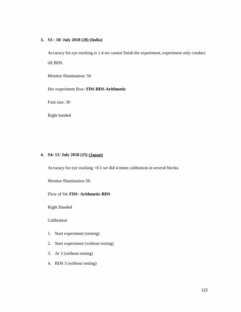
122

3. S3 : 10/ July 2018 (28) (India)

Accuracy for eye tracking is 1.4 we cannot finish the experiment, experiment only conduct

till BDS.

Monitor illumination: 50

Her experiment flow: FDS-BDS-Arithmetic

Font size: 30

Right handed

4. S4: 11/ July 2018 (25) (Japan)

Accuracy for eye tracking <0.5 we did 4 times calibration in several blocks.

Monitor Illumination 50.

Flow of S4: FDS- Arithmetic-BDS

Right Handed

Calibration

1. Start experiment (resting)

2. Start experiment (without resting)

3. Ar 3 (without resting)

4. BDS 3 (without resting)

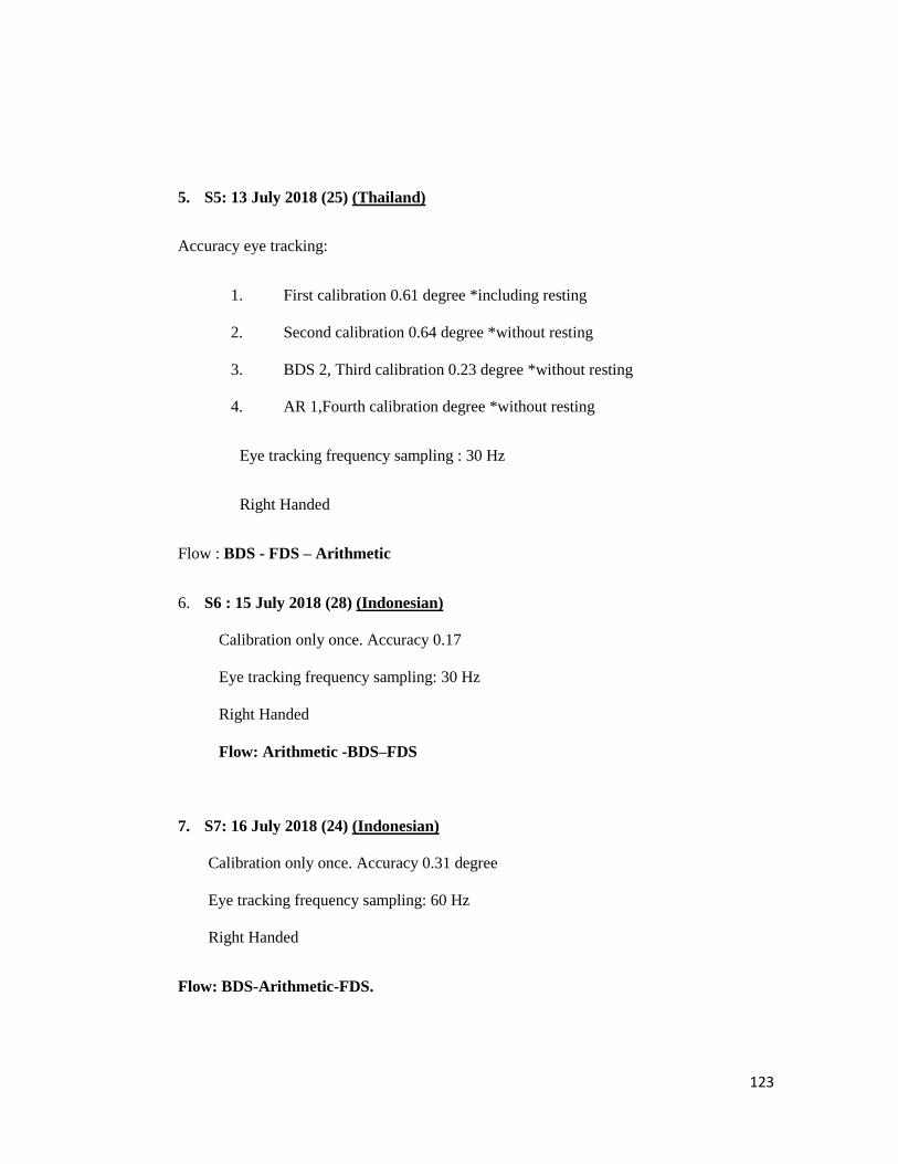
123

5. S5: 13 July 2018 (25) (Thailand)

Accuracy eye tracking:

1. First calibration 0.61 degree *including resting

2. Second calibration 0.64 degree *without resting

3. BDS 2, Third calibration 0.23 degree *without resting

4. AR 1,Fourth calibration degree *without resting

Eye tracking frequency sampling : 30 Hz

Right Handed

Flow : BDS - FDS – Arithmetic

6. S6 : 15 July 2018 (28) (Indonesian)

Calibration only once. Accuracy 0.17

Eye tracking frequency sampling: 30 Hz

Right Handed

Flow: Arithmetic -BDS–FDS

7. S7: 16 July 2018 (24) (Indonesian)

Calibration only once. Accuracy 0.31 degree


Right Handed

Flow: BDS-Arithmetic-FDS.

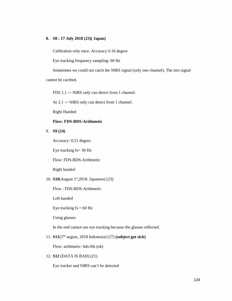
124

8. S8 : 17 July 2018 (23)( Japan)

Calibration only once. Accuracy 0.16 degree


Sometimes we could not catch the NIRS signal (only one channel). The nirs signal

cannot be cacthed.

FDS 1.1 -> NIRS only can detect from 1 channel.

Ar 2.1 -> NIRS only can detect from 1 channel.

Right Handed

Flow: FDS-BDS-Arithmetic

9. S9 (24)

Accuracy: 0.21 degree.

Eye tracking fs= 30 Hz

Flow: FDS-BDS-Arithmetic

Right handed

10. S10(August 1st,2018. Japanese) (23)

Flow : FDS-BDS-Arithmetic

Left handed

Eye tracking fs = 60 Hz

Using glasses

In the end cannot use eye tracking because the glasses reflected.

11. S11(2nd august, 2018 Indonesia) (27) (subject got sick)

Flow: arithmetic- bds-fds (ok)

12. S12 (DATA IS BAD) (21)

Eye tracker and NIRS can’t be detected

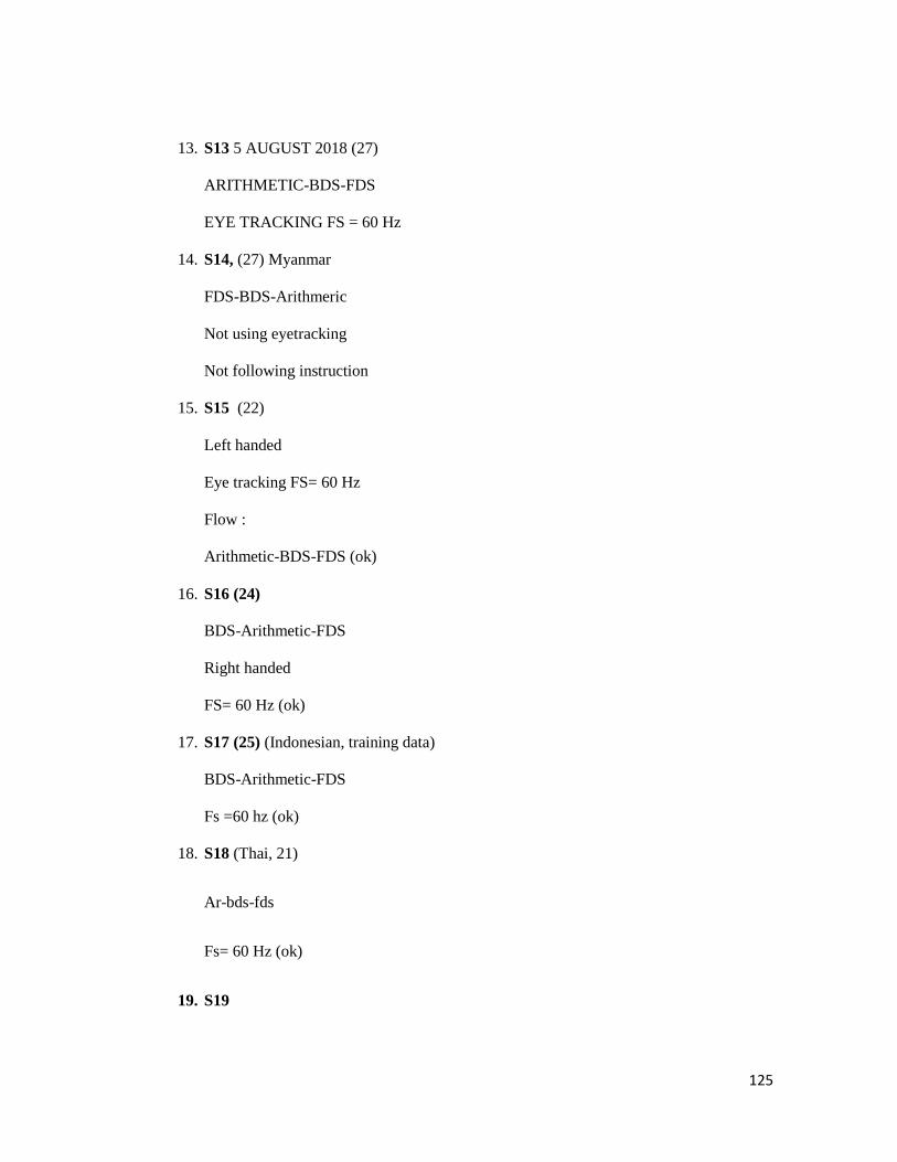
125

13. S13 5 AUGUST 2018 (27)

ARITHMETIC-BDS-FDS

EYE TRACKING FS = 60 Hz

14. S14, (27) Myanmar

FDS-BDS-Arithmeric

Not using eyetracking

Not following instruction

15. S15 (22)

Left handed

Eye tracking FS= 60 Hz

Flow :

Arithmetic-BDS-FDS (ok)

16. S16 (24)

BDS-Arithmetic-FDS

Right handed

FS= 60 Hz (ok)

17. S17 (25) (Indonesian, training data)

BDS-Arithmetic-FDS

Fs =60 hz (ok)

18. S18 (Thai, 21)

Ar-bds-fds

Fs= 60 Hz (ok)

19. S19

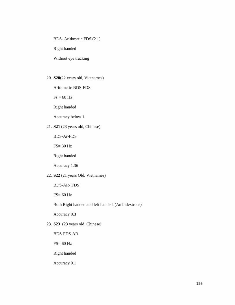
126

BDS- Arithmetic FDS (21 )

Right handed

Without eye tracking

20. S20(22 years old, Vietnames)

Arithmetic-BDS-FDS

Fs = 60 Hz

Right handed

Accuracy below 1.

21. S21 (23 years old, Chinese)

BDS-Ar-FDS

FS= 30 Hz

Right handed

Accuracy 1.36

22. S22 (21 years Old, Vietnames)

BDS-AR- FDS

FS= 60 Hz

Both Right handed and left handed. (Ambidextrous)

Accuracy 0.3

23. S23 (23 years old, Chinese)

BDS-FDS-AR

FS= 60 Hz

Right handed

Accuracy 0.1

127

24. S24 (28 years old, Indonesian)

BDS-FDS-AR

FS= 60 Hz

Right handed

Accuracy 0.9

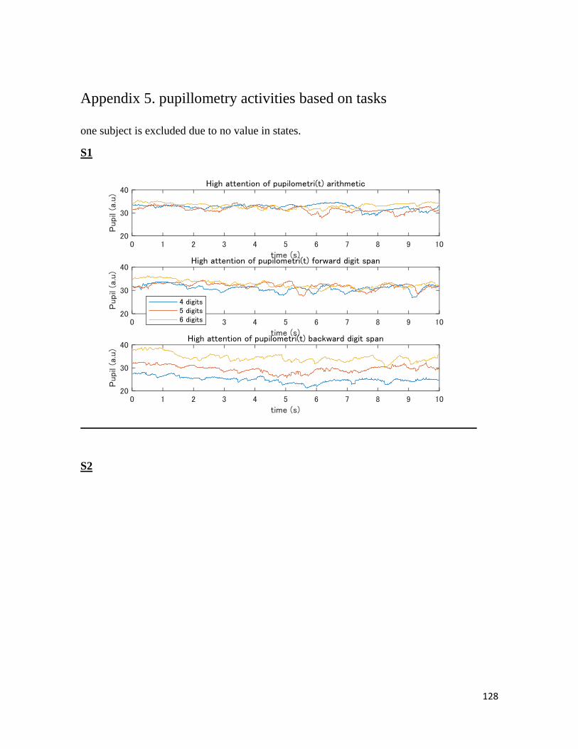
128

Appendix 5. pupillometry activities based on tasks

one subject is excluded due to no value in states.

S1

S2

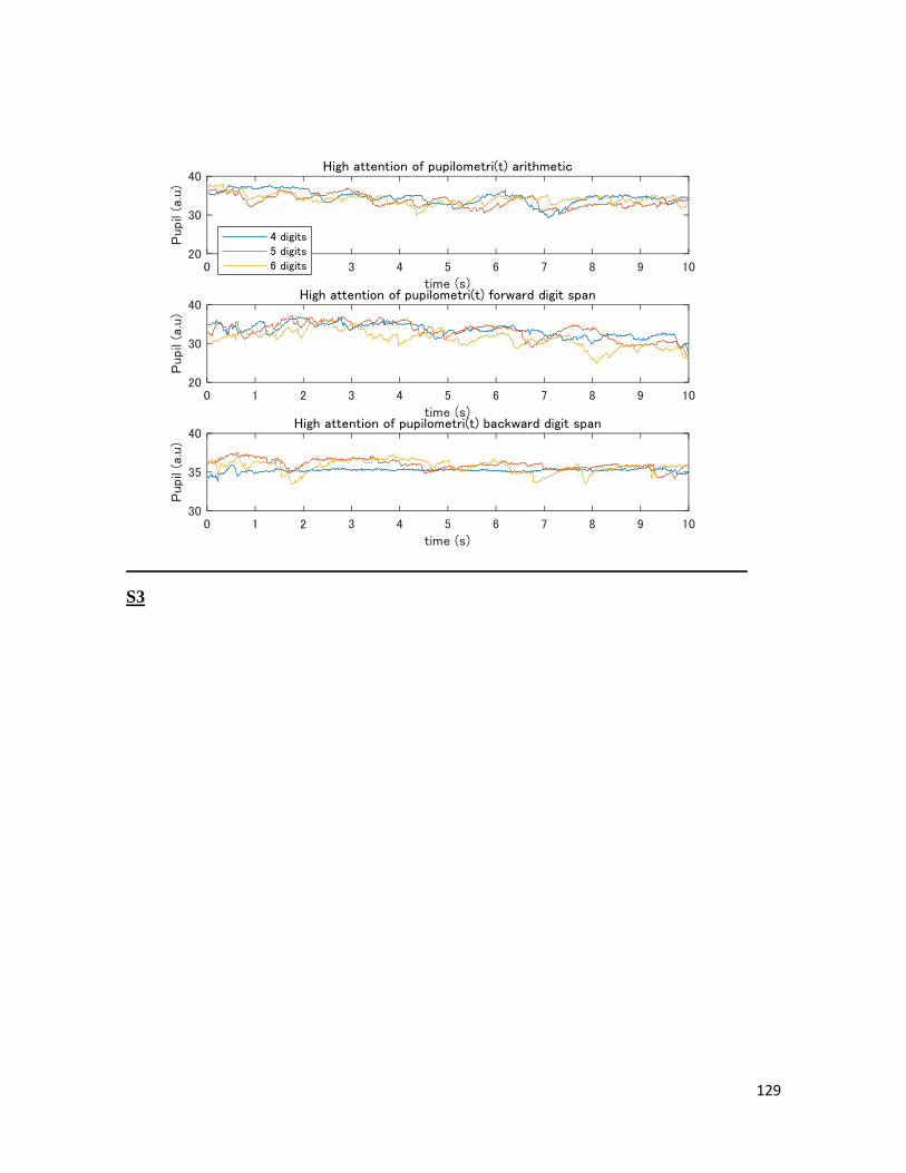
129

S3

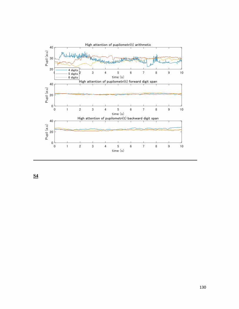
130

S4

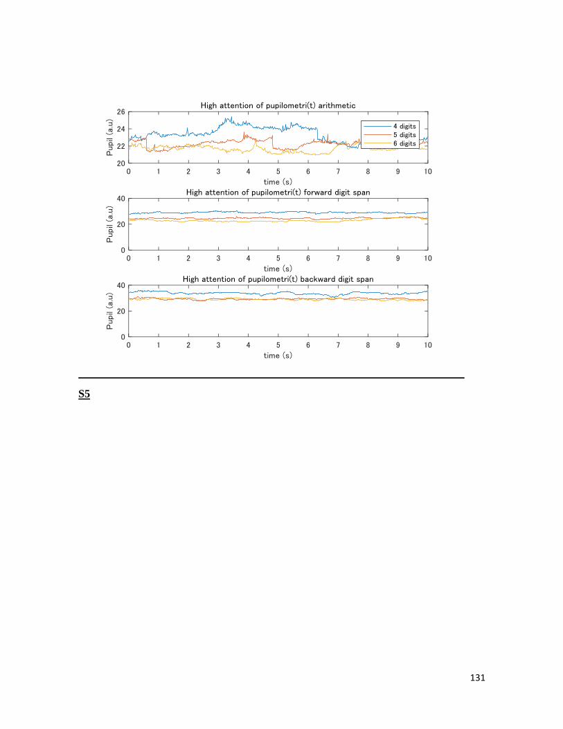
131

S5

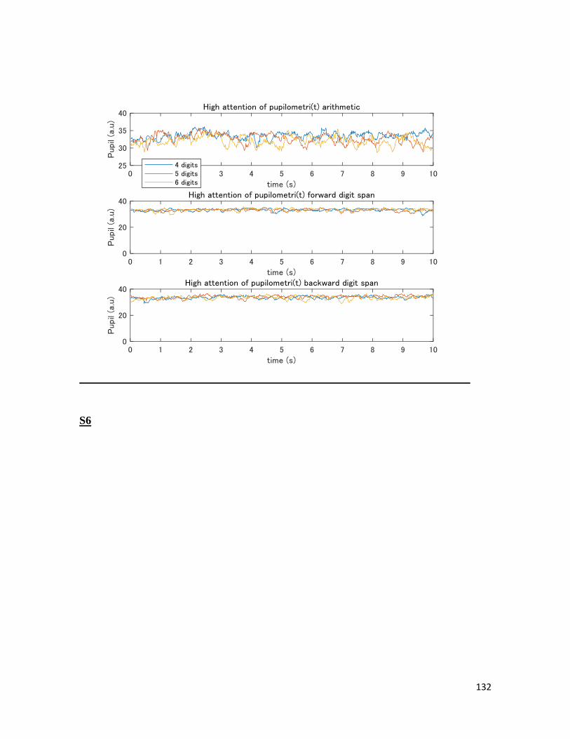
132

S6

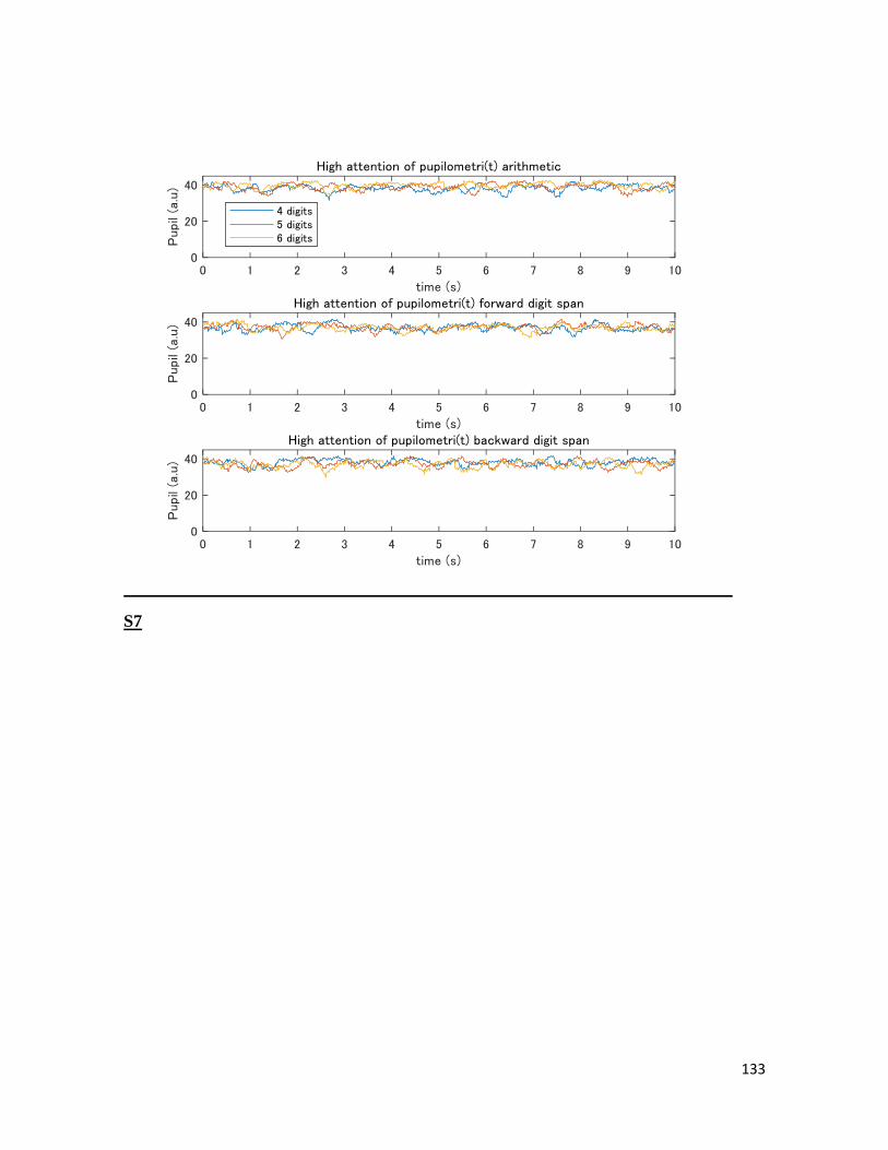
133

S7

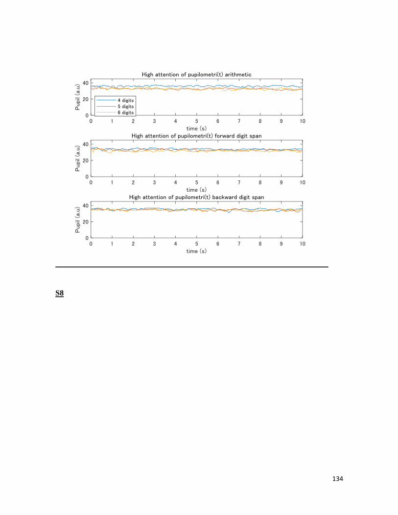
134

S8

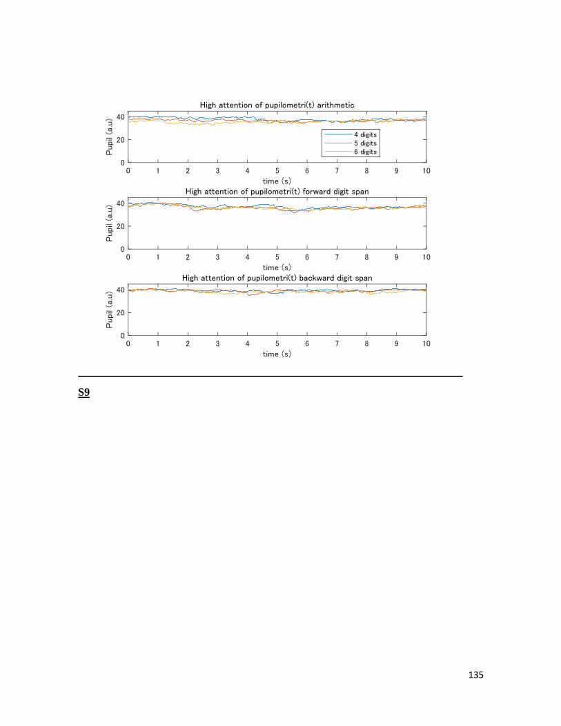
135

S9

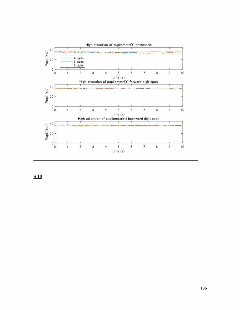
136

S 10

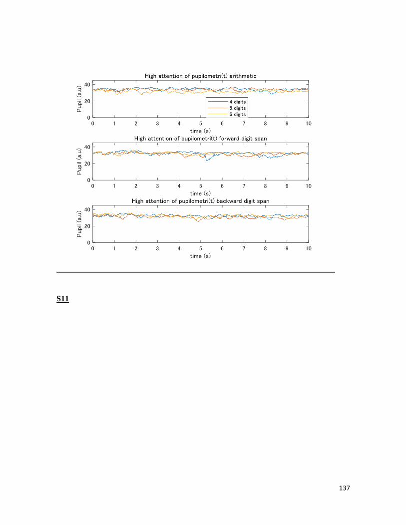
137

S11

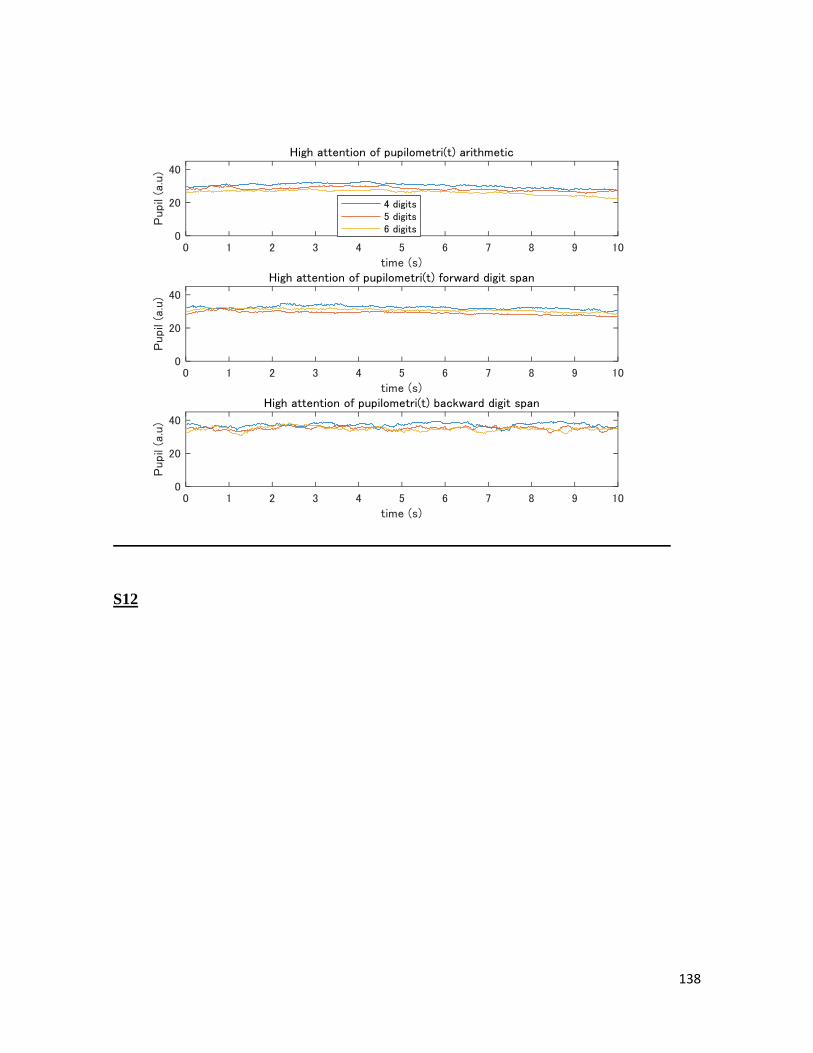
138

S12

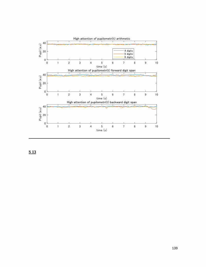
139

S 13

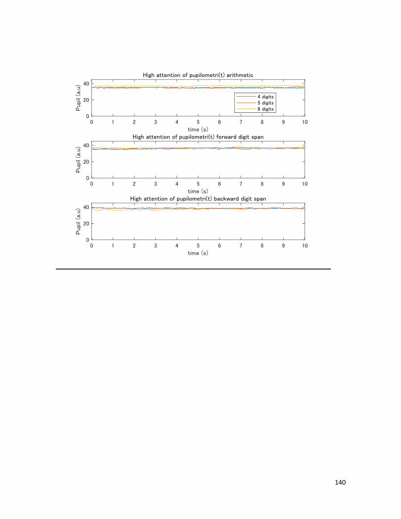
140

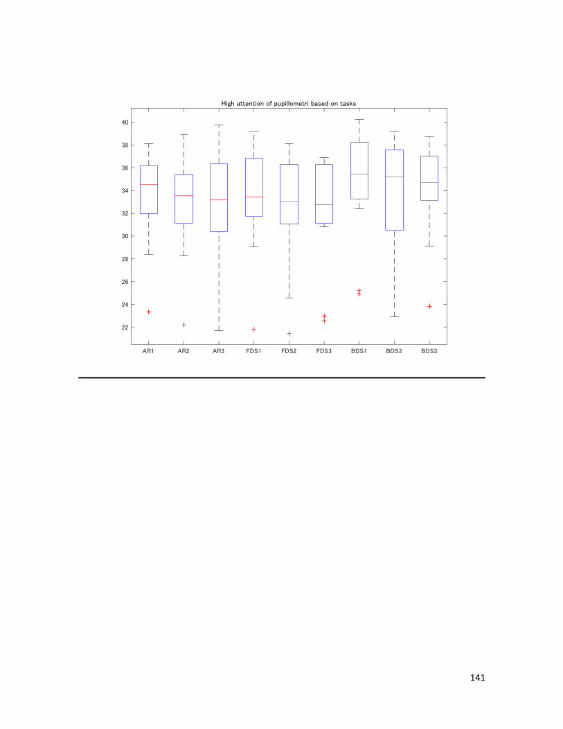
141

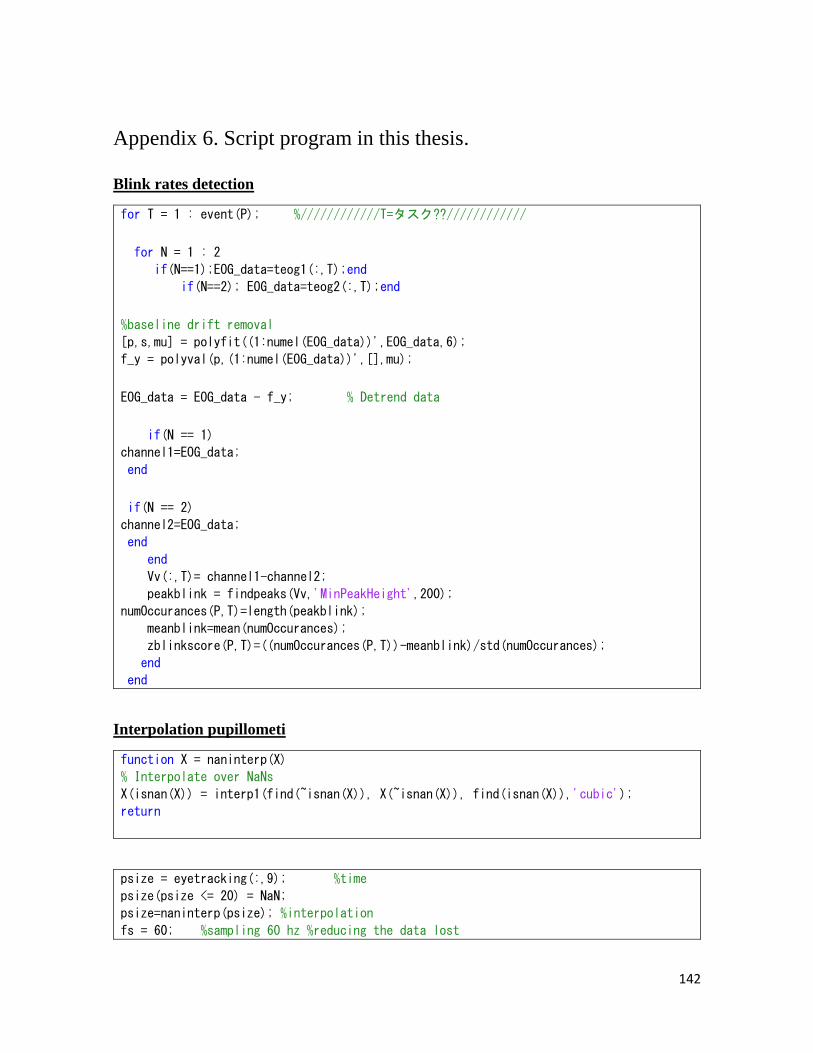
142

Appendix 6. Script program in this thesis.

Blink rates detection

for T = 1 : event(P); %////////////T=タスク??//////////// for N = 1 : 2 if(N==1);EOG_data=teog1(:,T);end if(N==2); EOG_data=teog2(:,T);end %baseline drift removal [p,s,mu] = polyfit((1:numel(EOG_data))',EOG_data,6); f_y = polyval(p,(1:numel(EOG_data))',[],mu); EOG_data = EOG_data - f_y; % Detrend data if(N == 1) channel1=EOG_data; end if(N == 2) channel2=EOG_data; end end Vv(:,T)= channel1-channel2; peakblink = findpeaks(Vv,'MinPeakHeight',200);

numOccurances(P,T)=length(peakblink); meanblink=mean(numOccurances); zblinkscore(P,T)=((numOccurances(P,T))-meanblink)/std(numOccurances); end end

Interpolation pupillometi

function X = naninterp(X) % Interpolate over NaNs X(isnan(X)) = interp1(find(~isnan(X)), X(~isnan(X)), find(isnan(X)),'cubic'); return

psize = eyetracking(:,9); %time psize(psize <= 20) = NaN; psize=naninterp(psize); %interpolation fs = 60; %sampling 60 hz %reducing the data lost

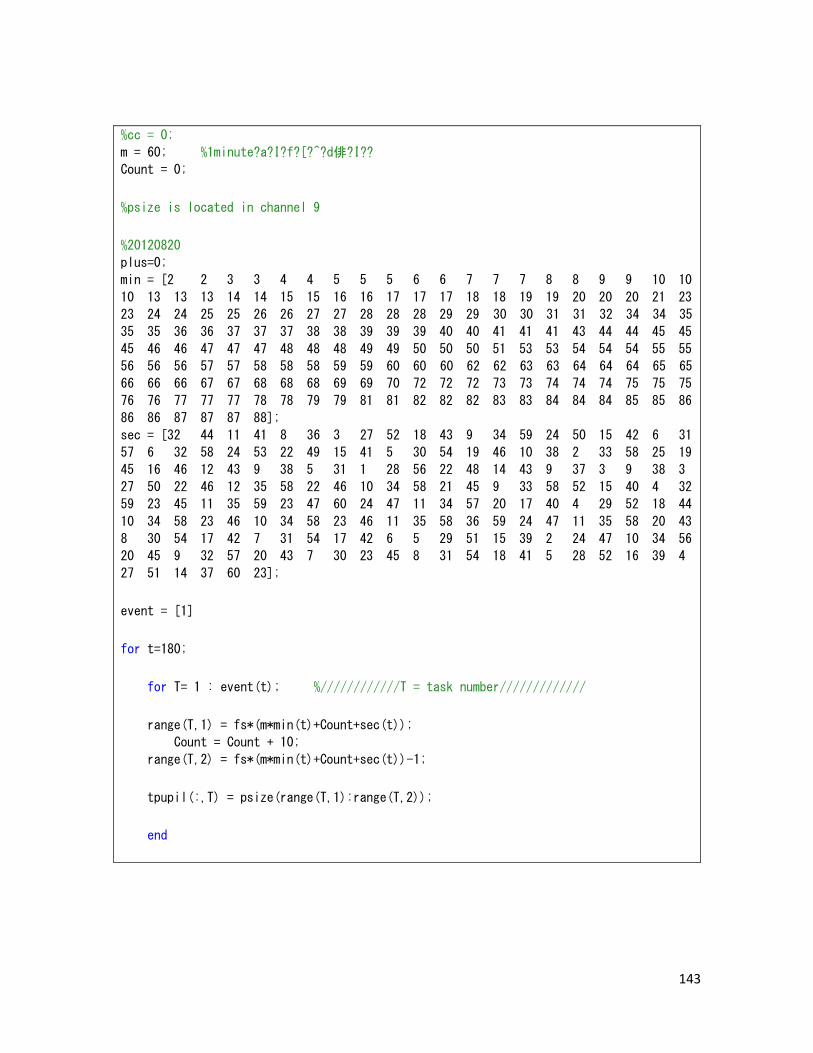
143

%cc = 0; m = 60; %1minute?a?I?f?[?^?d俳?I?? Count = 0; %psize is located in channel 9 %20120820 plus=0; min = [2 2 3 3 4 4 5 5 5 6 6 7 7 7 8 8 9 9 10 10

10 13 13 13 14 14 15 15 16 16 17 17 17 18 18 19 19 20 20 20 21 23

23 24 24 25 25 26 26 27 27 28 28 28 29 29 30 30 31 31 32 34 34 35

35 35 36 36 37 37 37 38 38 39 39 39 40 40 41 41 41 43 44 44 45 45

45 46 46 47 47 47 48 48 48 49 49 50 50 50 51 53 53 54 54 54 55 55

56 56 56 57 57 58 58 58 59 59 60 60 60 62 62 63 63 64 64 64 65 65

66 66 66 67 67 68 68 68 69 69 70 72 72 72 73 73 74 74 74 75 75 75

76 76 77 77 77 78 78 79 79 81 81 82 82 82 83 83 84 84 84 85 85 86

86 86 87 87 87 88]; sec = [32 44 11 41 8 36 3 27 52 18 43 9 34 59 24 50 15 42 6 31

57 6 32 58 24 53 22 49 15 41 5 30 54 19 46 10 38 2 33 58 25 19

45 16 46 12 43 9 38 5 31 1 28 56 22 48 14 43 9 37 3 9 38 3

27 50 22 46 12 35 58 22 46 10 34 58 21 45 9 33 58 52 15 40 4 32

59 23 45 11 35 59 23 47 60 24 47 11 34 57 20 17 40 4 29 52 18 44

10 34 58 23 46 10 34 58 23 46 11 35 58 36 59 24 47 11 35 58 20 43

8 30 54 17 42 7 31 54 17 42 6 5 29 51 15 39 2 24 47 10 34 56

20 45 9 32 57 20 43 7 30 23 45 8 31 54 18 41 5 28 52 16 39 4

27 51 14 37 60 23]; event = [1] for t=180; for T= 1 : event(t); %////////////T = task number///////////// range(T,1) = fs*(m*min(t)+Count+sec(t));

Count = Count + 10; range(T,2) = fs*(m*min(t)+Count+sec(t))-1; tpupil(:,T) = psize(range(T,1):range(T,2)); end

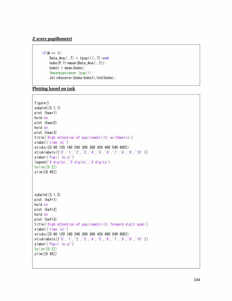
144

Z score pupillometri

if(N == 1); Data_Ana(:,T) = tpupil(:,T);end bobo(P,T)=mean(Data_Ana(:,T)); bobo1 = mean(bobo); %meanpups=mean (pupil); zblinkscore=(bobo-bobo1)/std(bobo);

Plotting based on task

figure() subplot(3,1,1) plot (haar1) hold on plot (haar2) hold on plot (haar3) title('High attention of pupilometri(t) arithmetic') xlabel('time (s)') xticks([0 60 120 180 240 300 360 420 480 540 600]) xticklabels({'0','1','2','3','4','5','6','7','8','9','10' }) ylabel('Pupil (a.u)') legend('4 digits','5 digits','6 digits') %xlim([0 2]) ylim([0 45])

subplot(3,1,2) plot (hafr1) hold on plot (hafr2) hold on plot (hafr3) title('High attention of pupilometri(t) forward digit span') xlabel('time (s)') xticks([0 60 120 180 240 300 360 420 480 540 600]) xticklabels({'0','1','2','3','4','5','6','7','8','9','10' }) ylabel('Pupil (a.u)') %xlim([0 2]) ylim([0 45])

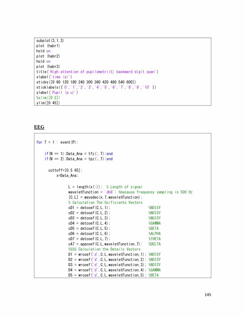
145

subplot(3,1,3) plot (habr1) hold on plot (habr2) hold on plot (habr3) title('High attention of pupilometri(t) backward digit span') xlabel('time (s)') xticks([0 60 120 180 240 300 360 420 480 540 600]) xticklabels({'0','1','2','3','4','5','6','7','8','9','10' }) ylabel('Pupil (a.u)') %xlim([0 2]) ylim([0 45])

EEG

for T = 1 : event(P); if(N == 1);Data_Ana = tfz(:,T);end if(N == 2);Data_Ana = tpz(:,T);end cuttoff=[0.5 65]; x=Data_Ana; L = length(x(:)); % Length of signal waveletFunction = 'db8'; %because frequency sampling is 500 Hz [C,L] = wavedec(x,7,waveletFunction); % Calculation The Coificients Vectors cD1 = detcoef(C,L,1); %NOISY cD2 = detcoef(C,L,2); %NOISY cD3 = detcoef(C,L,3); %NOISY cD4 = detcoef(C,L,4); %GAMMA cD5 = detcoef(C,L,5); %BETA cD6 = detcoef(C,L,6); %ALPHA cD7 = detcoef(C,L,7); %THETA cA7 = appcoef(C,L,waveletFunction,7); %DELTA %%%% Calculation the Details Vectors D1 = wrcoef('d',C,L,waveletFunction,1); %NOISY D2 = wrcoef('d',C,L,waveletFunction,2); %NOISY D3 = wrcoef('d',C,L,waveletFunction,3); %NOISY D4 = wrcoef('d',C,L,waveletFunction,4); %GAMMA D5 = wrcoef('d',C,L,waveletFunction,5); %BETA

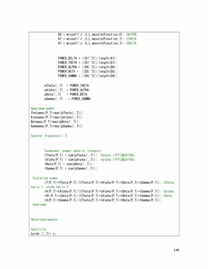
146

D6 = wrcoef('d',C,L,waveletFunction,6); %ALPHA D7 = wrcoef('d',C,L,waveletFunction,7); %THETA A7 = wrcoef('a',C,L,waveletFunction,7); %DELTA

POWER_DELTA = ((A7.^2))/length(A7); POWER_THETA = ((D7.^2))/length(D7); POWER_ALPHA = ((D6.^2))/length(D6); POWER_BETA = ((D5.^2))/length(D5); POWER_GAMMA = ((D4.^2))/length(D4); pTheta(:,T) = POWER_THETA; pAlpha(:,T) = POWER_ALPHA; pBeta(:,T) = POWER_BETA; pGamma(:,T) = POWER_GAMMA; %maximum power Thetamax(P,T)=max(pTheta(:,T)); Alphamax(P,T)=max(pAlpha(:,T)); Betamax(P,T)=max(pBeta(:,T)); Gammamax(P,T)=max(pGamma(:,T)); %center frequency(:,T)

%sumpower (power density integral) tTheta(P,T) = sum(pTheta(:,T)); %theta パ??[値の?㈹v tAlpha(P,T) = sum(pAlpha(:,T)); %alpha パ??[値の?㈹v tBeta(P,T) = sum(pBeta(:,T)); tGamma(P,T) = sum(pGamma(:,T)); %relative power rT(P,T)=tTheta(P,T)/(tTheta(P,T)+tAlpha(P,T)+tBeta(P,T)+tGamma(P,T)); %theta

baris 1, study baris 2 rA(P,T)=tAlpha(P,T)/(tTheta(P,T)+tAlpha(P,T)+tBeta(P,T)+tGamma(P,T)); %alpha rB1(P,T)=tBeta(P,T)/(tTheta(P,T)+tAlpha(P,T)+tBeta(P,T)+tGamma(P,T)); %beta rG(P,T)=tGamma(P,T)/(tTheta(P,T)+tAlpha(P,T)+tBeta(P,T)+tGamma(P,T)); %maximum

%Hjorthparameter %activity boleh (:,T)= x;

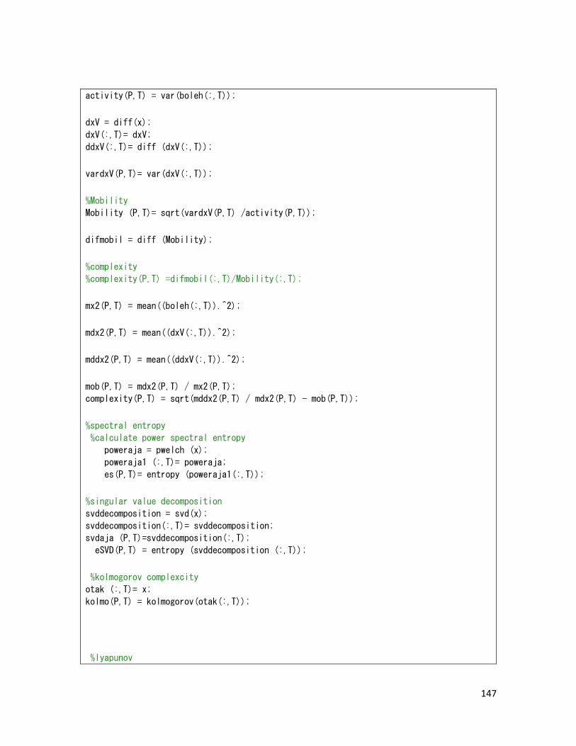
147

activity(P,T) = var(boleh(:,T)); dxV = diff(x); dxV(:,T)= dxV; ddxV(:,T)= diff (dxV(:,T)); vardxV(P,T)= var(dxV(:,T)); %Mobility Mobility (P,T)= sqrt(vardxV(P,T) /activity(P,T)); difmobil = diff (Mobility); %complexity %complexity(P,T) =difmobil(:,T)/Mobility(:,T); mx2(P,T) = mean((boleh(:,T)).^2); mdx2(P,T) = mean((dxV(:,T)).^2); mddx2(P,T) = mean((ddxV(:,T)).^2); mob(P,T) = mdx2(P,T) / mx2(P,T); complexity(P,T) = sqrt(mddx2(P,T) / mdx2(P,T) - mob(P,T));

%spectral entropy %calculate power spectral entropy poweraja = pwelch (x); poweraja1 (:,T)= poweraja; es(P,T)= entropy (poweraja1(:,T)); %singular value decomposition svddecomposition = svd(x); svddecomposition(:,T)= svddecomposition; svdaja (P,T)=svddecomposition(:,T); eSVD(P,T) = entropy (svddecomposition (:,T));

%kolmogorov complexcity otak (:,T)= x; kolmo(P,T) = kolmogorov(otak(:,T));

%lyapunov

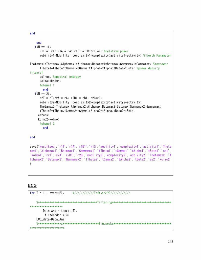
148

end end if(N == 1); r1T = rT; r1A = rA; r1B1 = rB1;r1G=rG;%relative power mobility1=Mobility; complexity1=complexity;activity1=activity; %Hjorth Parameter

Thetamax1=Thetamax;Alphamax1=Alphamax;Betamax1=Betamax;Gammamax1=Gammamax; %maxpower tTheta1=tTheta;tGamma1=tGamma;tAlpha1=tAlpha;tBeta1=tBeta; %power density

integral es1=es; %spectral entropy kolmo1=kolmo; %chanel 1 end if(N == 2); r2T = rT;r2A = rA; r2B1 = rB1; r2G=rG; mobility2=Mobility; complexity2=complexity;activity2=activity; Thetamax2=Thetamax;Alphamax2=Alphamax;Betamax2=Betamax;Gammamax2=Gammamax; tTheta2=tTheta;tGamma2=tGamma;tAlpha2=tAlpha;tBeta2=tBeta; es2=es; kolmo2=kolmo; %chanel 2 end end save('resulteeg','r1T','r1A','r1B1','r1G','mobility1','complexity1','activity1','Theta

max1','Alphamax1','Betamax1','Gammamax1','tTheta1','tGamma1','tAlpha1','tBeta1','es1',

'kolmo1','r2T','r2A','r2B1','r2G','mobility2','complexity2','activity2','Thetamax2','A

lphamax2','Betamax2','Gammamax2','tTheta2','tGamma2','tAlpha2','tBeta2','es2','kolmo2'

)

ECG

for T = 1 : event(P); %////////////T=タスク??////////////

%************************************filtering************************************

******************** Data_Ana = tecg(:,T); filteroder = 3; ECG_data=Data_Ana; %**************x**********************findpeaks***********************************

*********************

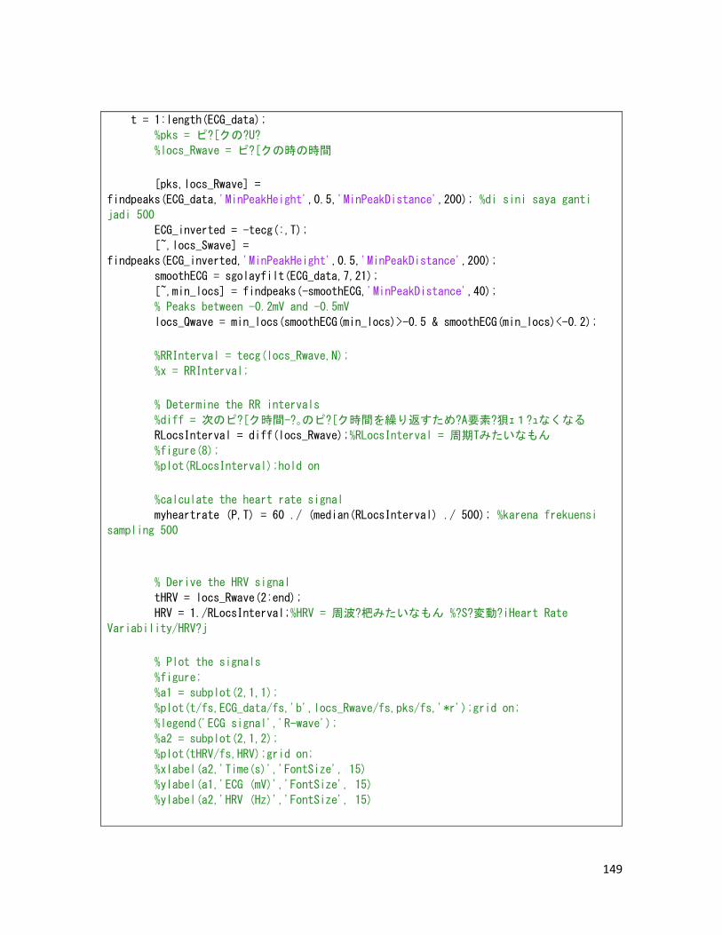
149

t = 1:length(ECG_data); %pks = ピ?[クの?U? %locs_Rwave = ピ?[クの時の時間 [pks,locs_Rwave] =

findpeaks(ECG_data,'MinPeakHeight',0.5,'MinPeakDistance',200); %di sini saya ganti

jadi 500 ECG_inverted = -tecg(:,T); [~,locs_Swave] =

findpeaks(ECG_inverted,'MinPeakHeight',0.5,'MinPeakDistance',200); smoothECG = sgolayfilt(ECG_data,7,21); [~,min_locs] = findpeaks(-smoothECG,'MinPeakDistance',40); % Peaks between -0.2mV and -0.5mV locs_Qwave = min_locs(smoothECG(min_locs)>-0.5 & smoothECG(min_locs)<-0.2);

%RRInterval = tecg(locs_Rwave,N); %x = RRInterval; % Determine the RR intervals %diff = 次のピ?[ク時間-?｡のピ?[ク時間を繰り返すため?A要素?狽ｪ１?ｭなくなる RLocsInterval = diff(locs_Rwave);%RLocsInterval = 周期Tみたいなもん %figure(8); %plot(RLocsInterval);hold on %calculate the heart rate signal myheartrate (P,T) = 60 ./ (median(RLocsInterval) ./ 500); %karena frekuensi

sampling 500

% Derive the HRV signal tHRV = locs_Rwave(2:end); HRV = 1./RLocsInterval;%HRV = 周波?杷みたいなもん %?S?変動?iHeart Rate

Variability/HRV?j % Plot the signals %figure; %a1 = subplot(2,1,1); %plot(t/fs,ECG_data/fs,'b',locs_Rwave/fs,pks/fs,'*r');grid on; %legend('ECG signal','R-wave'); %a2 = subplot(2,1,2); %plot(tHRV/fs,HRV);grid on; %xlabel(a2,'Time(s)','FontSize', 15) %ylabel(a1,'ECG (mV)','FontSize', 15) %ylabel(a2,'HRV (Hz)','FontSize', 15)

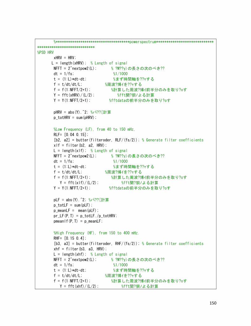
150

%************************************powerspectrum****************************

**************************** %PSD HRV xHRV = HRV; L = length(xHRV); % Length of signal NFFT = 2^nextpow2(L); % ?M??y)の長さの次のべき?? dt = 1/fs; %1/1000 t = (1:L)*dt-dt; %まず時間軸を??ｬする f = t/dt/dt/L; %周波?博ｲを??ｬする f = f(1:NFFT/2+1); %計算した周波?博ｲ前半分のみを取り?oす Y = fft(xHRV)/(L/2); %fft関?狽ﾉよる計算 Y = Y(1:NFFT/2+1); %fftdataの前半分のみを取り?oす

pHRV = abs(Y).^2; %パ??[計算 p_totHRV = sum(pHRV); %Low Frequency (LF), from 40 to 150 mHz, RLF= [0.04 0.15]; [b2, a2] = butter(filteroder, RLF/(fs/2)); % Generate filter coefficients xlf = filter(b2, a2, HRV); L = length(xlf); % Length of signal NFFT = 2^nextpow2(L); % ?M??y)の長さの次のべき?? dt = 1/fs; %1/1000 t = (1:L)*dt-dt; %まず時間軸を??ｬする f = t/dt/dt/L; %周波?博ｲを??ｬする f = f(1:NFFT/2+1); %計算した周波?博ｲ前半分のみを取り?oす Y = fft(xlf)/(L/2); %fft関?狽ﾉよる計算 Y = Y(1:NFFT/2+1); %fftdataの前半分のみを取り?oす pLF = abs(Y).^2; %パ??[計算 p_totLF = sum(pLF); p_meanLF = mean(pLF); pr_LF(P,T) = p_totLF./p_totHRV; pmeanlf(P,T) = p_meanLF; %High Frequency (HF), from 150 to 400 mHz. RHF= [0.15 0.4]; [b3, a3] = butter(filteroder, RHF/(fs/2)); % Generate filter coefficients xhf = filter(b3, a3, HRV); L = length(xhf); % Length of signal NFFT = 2^nextpow2(L); % ?M??y)の長さの次のべき?? dt = 1/fs; %1/1000 t = (1:L)*dt-dt; %まず時間軸を??ｬする f = t/dt/dt/L; %周波?博ｲを??ｬする f = f(1:NFFT/2+1); %計算した周波?博ｲ前半分のみを取り?oす Y = fft(xhf)/(L/2); %fft関?狽ﾉよる計算

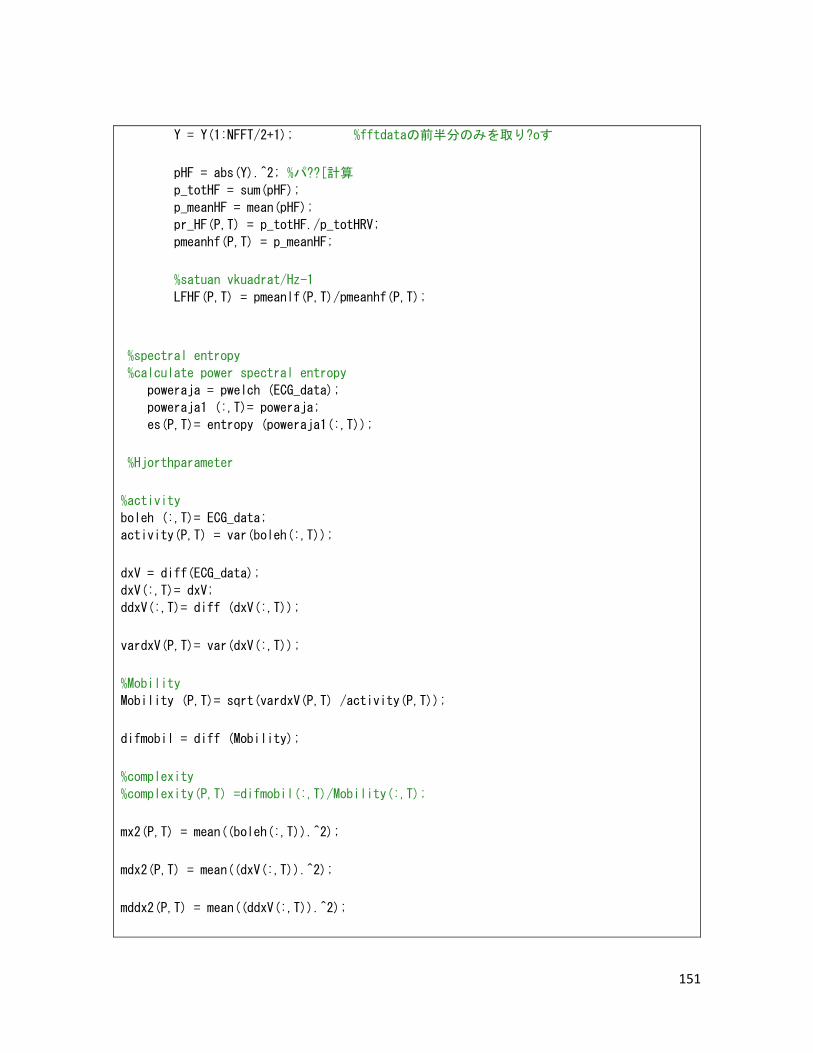
151

Y = Y(1:NFFT/2+1); %fftdataの前半分のみを取り?oす pHF = abs(Y).^2; %パ??[計算 p_totHF = sum(pHF); p_meanHF = mean(pHF); pr_HF(P,T) = p_totHF./p_totHRV; pmeanhf(P,T) = p_meanHF; %satuan vkuadrat/Hz-1 LFHF(P,T) = pmeanlf(P,T)/pmeanhf(P,T);

%spectral entropy %calculate power spectral entropy poweraja = pwelch (ECG_data); poweraja1 (:,T)= poweraja; es(P,T)= entropy (poweraja1(:,T)); %Hjorthparameter %activity boleh (:,T)= ECG_data; activity(P,T) = var(boleh(:,T)); dxV = diff(ECG_data); dxV(:,T)= dxV; ddxV(:,T)= diff (dxV(:,T)); vardxV(P,T)= var(dxV(:,T)); %Mobility Mobility (P,T)= sqrt(vardxV(P,T) /activity(P,T)); difmobil = diff (Mobility); %complexity %complexity(P,T) =difmobil(:,T)/Mobility(:,T); mx2(P,T) = mean((boleh(:,T)).^2); mdx2(P,T) = mean((dxV(:,T)).^2); mddx2(P,T) = mean((ddxV(:,T)).^2);

152

mob(P,T) = mdx2(P,T) / mx2(P,T); complexity(P,T) = sqrt(mddx2(P,T) / mdx2(P,T) - mob(P,T)); %singular value decomposition svddecomposition = svd(ECG_data); svddecomposition(:,T)= svddecomposition; svdaja (P,T)=svddecomposition(:,T); eSVD(P,T) = entropy (svdaja (P,T)); %kolmogorov entropy jantung (:,T)= tecg; kolmo(P,T) = kolmogorov(jantung(:,T)); end end

save('resultecg','complexity','Mobility','activity','es','pmeanhf','myheartrate','kolm

o')

NIRS

Data_Ana = tc1oxy(20:122,T);

%Hjorthparameter %activity activityoxy1(:,T) = var(Data_Ana); dxV = diff(Data_Ana); dxV(:,T)= dxV; ddxV(:,T)= diff (dxV(:,T)); vardxV(:,T)= var(dxV(:,T)); %Mobility Mobilityoxy1 (:,T)= sqrt(vardxV(:,T) ./activityoxy1(:,T)); difmobil = diff (Mobilityoxy1); %complexity %complexity(P,T) =difmobil(:,T)/Mobility(:,T); mx2(:,T) = mean((Data_Ana).^2);

153

mdx2(:,T) = mean((dxV(:,T)).^2); mddx2(:,T) = mean((ddxV(:,T)).^2); mob(:,T) = mdx2(:,T) ./ mx2(:,T); complexityoxy1(:,T) = sqrt(mddx2(:,T) ./ mdx2(:,T) - mob(:,T));

end %Deoxyhemoglobin ch 1 for T = 1 : event(P); %////////////T=タスク??//////////// Data_Ana = tc1deoxy(20:122,T);

%Hjorthparameter %activity activitydeoxy1(:,T) = var(Data_Ana); dxV = diff(Data_Ana); dxV(:,T)= dxV; ddxV(:,T)= diff (dxV(:,T)); vardxV(:,T)= var(dxV(:,T)); %Mobility Mobilitydeoxy1 (:,T)= sqrt(vardxV(:,T) ./activitydeoxy1(:,T)); difmobil = diff (Mobilitydeoxy1); %complexity %complexity(P,T) =difmobil(:,T)/Mobility(:,T); mx2(:,T) = mean((Data_Ana).^2); mdx2(:,T) = mean((dxV(:,T)).^2); mddx2(:,T) = mean((ddxV(:,T)).^2); mob(:,T) = mdx2(:,T) ./ mx2(:,T); complexitydeoxy1(:,T) = sqrt(mddx2(:,T) ./ mdx2(:,T) - mob(:,T)); end %totalhemoglobin ch 1 for T = 1 : event(P); %////////////T=タスク??//////////// Data_Ana = tc1total(20:122,T); %Hjorthparameter %activity activitytot1(:,T) = var(Data_Ana); dxV = diff(Data_Ana); dxV(:,T)= dxV; ddxV(:,T)= diff (dxV(:,T)); vardxV(:,T)= var(dxV(:,T)); %Mobility Mobilitytot1 (:,T)= sqrt(vardxV(:,T) ./activitytot1(:,T)); difmobil = diff (Mobilitytot1); %complexity %complexity(P,T) =difmobil(:,T)/Mobility(:,T);

154

mx2(:,T) = mean((Data_Ana).^2); mdx2(:,T) = mean((dxV(:,T)).^2); mddx2(:,T) = mean((ddxV(:,T)).^2); mob(:,T) = mdx2(:,T) ./ mx2(:,T); complexitytot1(:,T) = sqrt(mddx2(:,T) ./ mdx2(:,T) - mob(:,T)); end %oxyhemoglobin ch 2 for T = 1 : event(P); %////////////T=タスク??//////////// Data_Ana = tc2oxy(20:122,T); %Hjorthparameter %activity activityoxy2(:,T) = var(Data_Ana); dxV = diff(Data_Ana); dxV(:,T)= dxV; ddxV(:,T)= diff (dxV(:,T)); vardxV(:,T)= var(dxV(:,T)); %Mobility Mobilityoxy2 (:,T)= sqrt(vardxV(:,T) ./activityoxy2(:,T)); difmobil = diff (Mobilityoxy2); %complexity %complexity(P,T) =difmobil(:,T)/Mobility(:,T); mx2(:,T) = mean((Data_Ana).^2); mdx2(:,T) = mean((dxV(:,T)).^2); mddx2(:,T) = mean((ddxV(:,T)).^2); mob(:,T) = mdx2(:,T) ./ mx2(:,T); complexityoxy2(:,T) = sqrt(mddx2(:,T) ./ mdx2(:,T) - mob(:,T)); end %deoxyhemoglobin ch 2 for T = 1 : event(P); %////////////T=タスク??//////////// Data_Ana = tc2deoxy(20:122,T); %Hjorthparameter %activity activitydeoxy2(:,T) = var(Data_Ana); dxV = diff(Data_Ana); dxV(:,T)= dxV; ddxV(:,T)= diff (dxV(:,T)); vardxV(:,T)= var(dxV(:,T)); %Mobility Mobilitydeoxy2 (:,T)= sqrt(vardxV(:,T) ./activitydeoxy2(:,T)); difmobil = diff (Mobilitydeoxy2); %complexity %complexity(:,T) =difmobil(:,T)/Mobility(:,T); mx2(:,T) = mean((Data_Ana).^2);

155

mdx2(:,T) = mean((dxV(:,T)).^2); mddx2(:,T) = mean((ddxV(:,T)).^2); mob(:,T) = mdx2(:,T) ./ mx2(:,T); complexitydeoxy2(:,T) = sqrt(mddx2(:,T) ./ mdx2(:,T) - mob(:,T)); end %total hemoglobin ch 2 for T = 1 : event(P); %////////////T=タスク??//////////// Data_Ana = tc2total(20:122,T); %Hjorth:arameter %activity activitytot2(:,T) = var(Data_Ana); dxV = diff(Data_Ana); dxV(:,T)= dxV; ddxV(:,T)= diff (dxV(:,T)); vardxV(:,T)= var(dxV(:,T)); %Mobility Mobilitytot2 (:,T)= sqrt(vardxV(:,T) ./activitytot2(:,T)); difmobil = diff (Mobilitytot2); %com:lexity %com:lexity(:,T) =difmobil(:,T)/Mobility(:,T); mx2(:,T) = mean((Data_Ana).^2); mdx2(:,T) = mean((dxV(:,T)).^2); mddx2(:,T) = mean((ddxV(:,T)).^2); mob(:,T) = mdx2(:,T) ./ mx2(:,T); complexitytot2(:,T) = sqrt(mddx2(:,T) ./ mdx2(:,T) - mob(:,T)); end

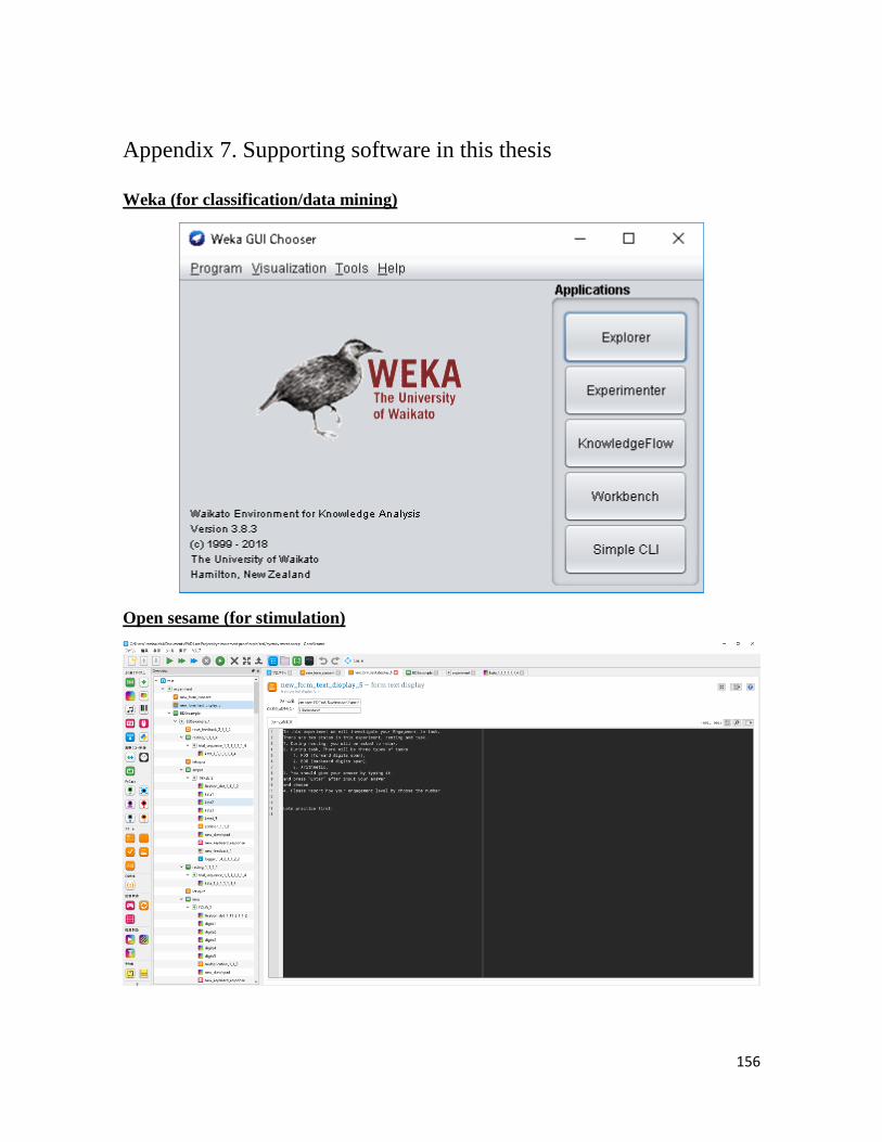
156

Appendix 7. Supporting software in this thesis

Weka (for classification/data mining)

Open sesame (for stimulation)

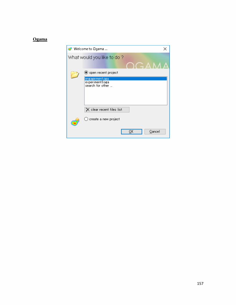
157

Ogama

Documents

Labelling Method by Pupillometry for Classifying Attention