Labor Market Rigidities, Trade and Unemployment∗

Elhanan HelpmanHarvard University and CIFAR

Oleg ItskhokiHarvard University

June 12, 2008

Abstract

We study a two-country two-sector model of international trade in which one sector produces

homogeneous products while the other produces differentiated products. The differentiated-

product industry has firm heterogeneity, monopolistic competition, search and matching in its

labor market, and wage bargaining. Some of the workers searching for jobs end up being unem-

ployed. Countries are similar except for frictions in their labor markets, which include efficiency

of matching, cost of vacancies, firing costs, and unemployment benefits. We study the interaction

of labor market rigidities and trade impediments in shaping welfare, trade flows, productivity,

and unemployment. We show that both countries gain from trade but that the flexible country–

which has lower labor market frictions–gains proportionately more. A flexible labor market

confers comparative advantage; the flexible country exports differentiated products on net. A

country benefits from lowering frictions in its labor market, but this harms the country’s trade

partner. And the simultaneous proportional lowering of labor market frictions in both countries

benefits both of them. The model generates rich patterns of unemployment. In particular,

better labor market institutions do not ensure lower unemployment, and unemployment and

welfare can both rise in response to a policy change or falling trade costs.

Keywords: labor market frictions, unemployment, productivity, tradeJEL Classification: F12, F16, J64

∗We thank Alberto Alesina, Pol Antràs, Jonathan Eaton, Emmanuel Farhi, Larry Katz, Kala Krishna, DavidLaibson, and Stephen Redding for comments, Jane Trahan for editorial assistance, and Helpman thanks the NationalScience Foundation for financial support.

1 Introduction

International trade and international capital flows link national economies. Although such links are

considered to be beneficial for the most part, they produce an interdependence that occasionally

has harmful effects. In particular, shocks that emanate in one country may negatively impact trade

partners. On the trade side, links through terms-of-trade movements have been widely studied,

and it is now well understood that, say, capital accumulation or technological change can worsen a

trade partner’s terms of trade and reduce its welfare. On the macro side, the transmission of real

business cycles has been widely studied, such as the impact of technology shocks in one country on

income fluctuations in its trade partners.

Although a large literature addresses the relationship between trade and unemployment, we

fall short of understanding how these links depend on labor market institutions. There is growing

awareness that institutions affect comparative advantage and trade flows. Levchenko (2007), Nunn

(2007) and Costinot (2006) provide evidence on the impact of legal institutions, while Cuñat and

Melitz (2007) and Chor (2006) provide evidence on the impact of labor market institutions.

Indeed, measures of labor market flexibility developed by Botero et al. (2004) differ greatly

across countries.1 The rigidity of employment index, which is an average of three other indexes–

difficulty of hiring, difficulty of firing, and rigidity of hours–shows wide variation in its range

between zero and one hundred (where higher values represent larger rigidities). Importantly, coun-

tries with very different development levels may have similar labor market rigidities. For example,

Chad, Morocco and Spain have indexes of 60, 63 and 63, respectively, which are about twice the

average for the OECD countries (which is 33.3) and higher than the average for sub-Saharan Africa.

The United States has the lowest index, equal to zero, while Australia has an index of three and

New Zealand has an index of seven, all significantly below the OECD average. Yet some of the

much poorer countries also have very flexible labor markets, e.g., both Uganda and Togo have an

index of seven.

We develop in this paper a two-country model of international trade in order to study the

effects of labor market frictions on trade flows, productivity, welfare and unemployment. We are

particularly interested in the impact of a country’s labor market rigidities on its trade partner, and

the differential impact of lower trade impediments on countries with different labor market institu-

tions. Blanchard and Wolfers (2000) emphasize the need to allow for interactions between shocks

and differences in labor market institutions in order to explain the evolution of unemployment in

European economies. They show that these interactions are empirically important. On the other

side, Nickell et al. (2002) emphasize changes over time in labor market institutions as important

determinants of the evolution of unemployment in OECD countries. While these studies use rich

data on labor market institutions, our theoretical model parametrizes labor market rigidities in a

1Their original data has been updated by the World Bank and is now available athttp://www.doingbusiness.org/ExploreTopics/EmployingWorkers/. The numbers reported in the text comefrom this site, downloaded on May 20, 2007. It is important to note that other measures of labor marketcharacteristics are available for OECD countries; see Nickell (1997) and Blanchard and Wolfers (2000).

1

simple way, which can be related to a variety of labor market features, such as the cost of vacancies,

the efficiency of matching in labor markets, firing costs and unemployment insurance. We focus

the analysis on search and matching frictions in Sections 2-6, and show in Section 7 how the results

generalize to economies with firing costs and unemployment benefits. We show, however, that even

the simpler search and matching frictions generate rich patterns of unemployment in response to

both variation across countries in labor market rigidities and changes in trade impediments.

The literature on trade and unemployment is large and varied. One strand of this literature con-

siders economies with minimum wages, of which Brecher (1974) represents an early contribution.2

Another approach, due to Matusz (1986), uses implicit contracts. A third approach, exemplified

by Copland (1989), incorporates efficiency wages into trade models.3 Yet another line of research

uses fair wages. Agell and Lundborg (1995) and Kreickemeier and Nelson (2006) illustrate this

approach. The final approach uses search and matching in labor markets. While two early studies

extended the two-sector model of Jones (1965) to economies with this type of labor market fric-

tion,4 Davidson, Martin and Matusz (1999) provide a particularly valuable analysis of international

trade with labor markets that are characterized by Diamond-Mortensen-Pissarides-type search and

matching frictions.5 In their model differences in labor market frictions, both across sectors and

across countries, generate Ricardian-type comparative advantage.6

Our two-sector model incorporates Diamond-Mortensen-Pissarides-type frictions into a sector

that produces differentiated products; another sector manufactures homogeneous goods under con-

stant returns to scale. In the differentiated-product sector heterogeneous firms compete monop-

olistically, as in Melitz (2003). These firms exercise market power in the product market on the

one hand, and bargain with workers over wages on the other.7 As in models with home market

effects, it is costly to trade differentiated products. Moreover, there are fixed and variable trade

costs. While we conduct most of the analysis under the assumption that there is full employment

in the homogeneous sector, we show in Section 6 how the results generalize to economies with

unemployment in that sector.8

We develop the model in stages. The next section describes demand, product markets, labor

markets, and the determinants of wages and profits. In the following section, Section 3, we dis-

cuss the structure of equilibrium, focusing on the case in which both countries are incompletely

2His approach has been extended by Davis (1998) to study how wages are determined when two countries tradewith each other, one with and one without a minimum wage.

3See also Brecher (1992) and Hoon (2001).4See Davidson, Martin and Matusz (1988) and Hosios (1990).5See Pissarides (2000) for the theory of search and matching in labor markets.6More work has followed this line of inquiry than the other approaches mentioned in the text. Recent examples

include Davidson and Matusz (2006a, 2006b) and Moore and Ranjan (2005).7A surge of papers has incorporated labor market frictions into models with heterogeneous firms. Egger and

Kreickemeier (2006) examine trade liberalization in an environment with fair wages and Davis and Harrigan (2007)examine trade liberalization in an environment with efficiency wages; both papers focus on the wage dispersion ofidentical workers across heterogeneous firms in symmetric countries. Mitra and Ranjan (2007) examine offshoring inan environment with search and matching and Felbermayr, Prat and Schmerer (2008) study trade in a one-sectormodel with search and matching and symmetric countries.

8There we also show how the results generalize to economies with variable trade costs in the homogeneous sector.

2

specialized, and–as in Melitz (2003)–only a fraction of firms export in the differentiated-product

industries and some entrants exit those industries. This is followed by an analysis of the impact

of labor market frictions on trade, welfare, and productivity in Section 4. There we also study

the differential impact of lower trade impediments on countries with different labor market institu-

tions. Importantly, we show that both countries gain from trade in welfare terms and in terms of

total factor productivity, independently of trade costs and differences in labor market institutions.9

However, the country with lower frictions in the labor market gains from trade proportionately

more. The lowering of labor market frictions in one country raises its welfare, but it harms the

trade partner. Nevertheless, both countries benefit from simultaneous proportional improvements

in labor market institutions across the world.

By lower frictions in its labor market a country gains a competitive advantage in the differen-

tiated sector, which is reminiscence of a productivity improvement. As a result, it attracts more

firms into this sector while the foreign country attracts fewer firms into this sector. The entry and

exit of firms overwhelms the terms of trade movement, leading to welfare gains in the country with

improved labor market frictions and welfare losses in its trade partner.

In Section 4 we also show that labor market flexibility is a source of comparative advantage.

The flexible country has a larger fraction of exporting firms and it exports differentiated products

on net. Moreover, the share of intra-industry trade is smaller and the total volume of trade is larger

the larger are the differences in labor market rigidities. We also show that welfare and productivity

are higher in the more flexible country.

In Section 5 we take up unemployment. We show that the relationship between unemployment

and labor market rigidities is hump-shaped when the countries are symmetric. An improvement in

labor market institutions decreases the sectoral rate of unemployment and induces more workers to

search for jobs in the differentiated-product sector, which has the higher sectoral rate of unemploy-

ment. These two effects impact unemployment in opposite directions, with the latter dominating

in highly rigid labor markets and the former dominating in highly flexible labor markets. As a

result, unemployment initially increases and then decreases as labor market institutions improve,

starting from high levels of rigidity. We also show that if a single country improves its labor mar-

ket institutions this reduces unemployment in the country’s trading partner, by inducing a labor

reallocation from the differentiated-product sector to the homogeneous-product sector.

We also show that lowering trade impediments can increase unemployment in one or both

countries, despite its positive welfare effects, and that the interaction between trade impediments

and labor market rigidities produces rich patterns of unemployment. Specifically, differences in

rates of unemployment do not necessarily reflect differences in labor market institutions; the flexible

country can have higher or lower unemployment, depending on the height of trade impediments

and the levels of labor market frictions.9We also show that the combination of variable trade costs and differences in labor market institutions have to

satisfy a certain condition for the equilibrium to have incomplete specialization in both countries. However, thewelfare results extend to cases with partial or full specialization. Moreover, we show in Section 7 how these welfareresults have to be qualified in the presence of unemployment benefits.

3

The unemployment results depend on certain structural features of the model, while the welfare,

productivity, and trade pattern results are less sensitive to these characteristics. In particular, the

impact of trade liberalization on unemployment as a function of differences in labor market rigidities,

depends on the assumption that there are labor market rigidities in the differentiated-product sector

but not in the homogeneous-product sector. Under these circumstances trade liberalization induces

an expansion of activity in the sector with the higher sectoral rate of unemployment. These results

are generalized, in Section 6, by introducing unemployment into the homogeneous-product sector.

In particular, as long as the sectoral rate of unemployment is higher in the differentiated sector, the

results do not change. But in cases in which it is higher in the homogeneous sector, the response

of unemployment to shocks changes.

In Section 7 we add firing costs and unemployment benefits to the menu of labor market frictions,

and we discuss conditions under which the previous results remain valid, as well as how the results

change when these conditions are not satisfied. In addition, we analyze the impact of reforms in

firing costs and unemployment benefits on resource allocation, unemployment and welfare of the

reforming country and its trade partner. The last section summarizes some of the main insights

from this analysis.

2 Preliminaries

We develop in this section the building blocks of our analytical model. They consist of a demand

structure, technologies, product and labor market structures, and determinants of wages and prof-

its. After describing these ingredients in some detail, we discuss in the next two sections general

equilibrium interactions in a two-country world. In order to focus on labor market rigidities, we

assume that the two countries are identical except for labor market frictions. This means that the

demand structure and the technologies are the same in both countries. They can differ in the size

of their labor endowment, but this difference is not consequential for the type of equilibrium we

discuss in the main text.

2.1 Preferences and Demand

Every country has a representative agent who consumes a homogeneous product q0 and a continuum

of brands of a differentiated product whose real consumption index is Q. The real consumption

index of the differentiated product is a constant elasticity of substitution aggregator:

Q =

∙Zω∈Ω

q(ω)βdω

¸ 1β

, 0 < β < 1, (1)

where q (ω) represents the consumption of variety ω, Ω represents the set of varieties available for

consumption, and β is a parameter that controls the elasticity of substitution between brands.10

10Alternatively, we could interpret Q to be a homogeneous final product and the q (ω)s to be intermediate inputs.

4

Consumer preferences between the homogeneous product, q0, and the real consumption index

of the differentiated product, Q, are represented by the quasi-linear utility function11

U = q0 +1

ζQζ , 0 < ζ < β.

The restriction ζ < β ensures that varieties are better substitutes for each other than for the

outside good q0.12 We also assume that the consumer has a large enough income level to always

consume positive quantities of the outside good, in which case it is convenient to choose the outside

good as numeraire, so that its price equals one, i.e., p0 = 1. Under the circumstances p (ω), the

price of brand ω, and P , the price index of the brands, are measured relative to the price of the

homogeneous product.13

The utility function U implies that a consumer with spending E who faces the price index P

for the differentiated product chooses Q = P−1/(1−ζ) and q0 = E − P−ζ/(1−ζ).14 As a result, the

demand function for brand ω can be expressed as

q(ω) = Q−β−ζ1−β p(ω)−

11−β (2)

and the indirect utility function as

V = E +1− ζ

ζP−

ζ1−ζ = E +

1− ζ

ζQζ . (3)

As usual, the indirect utility function is increasing in spending and declining in price. A higher price

index P reduces the demand for Q, and–holding expenditure E constant–reduces welfare. This

decline in welfare results from the fact that consumer surplus, (1− ζ)P−ζ/(1−ζ)/ζ = (1− ζ)Qζ/ζ,

declines as P rises and Q falls. In what follows, we characterize equilibrium values of Q, from which

we infer welfare levels.

Note from (2) that the demand for every variety decreases in its own price and in the real

consumption index Q. The latter results from the fact that higher Q implies that the differentiated-

product market is more competitive, because the price index P is lower, and P is lower either

because prices of competing brands are lower or because there is more variety available in the

market.11Alternatively, we could use a homothetic utility function in q0 and Q; see Appendix for a discussion of this case.12This model can be analyzed without the restriction ζ > 0. This assumption, however, allows us to avoid discussing

alternative special cases and brings out some of the interesting results in a clear way.13The price index P is given by

P =ω∈Ω

p(ω)−β

1−β dω− 1−β

β

.

14The assumption that consumer spending on the outside good is positive is equivalent to assuming E > P−ζ/(1−ζ).Since ζ > 0, the demand for Q is elastic and total spending PQ rises when P falls.

5

2.2 Technologies and Market Structure

All goods are produced with labor, which is the only factor of production. The homogeneous

product requires one unit of labor per unit output and the market for this product is competitive.

When h0 workers are employed in the production of the homogeneous product, its output level

equals h0.

The market for brands of the differentiated product is monopolistically competitive. A firm

that seeks to supply a brand ω bears an entry cost fe in terms of the homogeneous good, which

covers the technology cost and the cost of setting up shop in the industry. After bearing this cost,

the firm learns how productive its technology is, as measured by θ; a θ-firm requires 1/θ workers

per unit output. In other words, if a θ-firm employs h workers it produces θh units of output.

Before entry the firm expects θ to be drawn from a known cumulative distribution Gθ (θ).

After entry the firm has to bear a fixed production cost fd in terms of the homogeneous good;

without it no manufacturing is possible. Following Melitz (2003), we assume that the differentiated-

product sector bears a fixed cost of exporting fx in terms of the homogeneous product. In addition,

it bears a variable cost of exporting of the melting-iceberg type: τ > 1 units have to be exported

for one unit to arrive in the foreign country. As is common in models with home market effects,

we assume that there are no trade frictions in the homogeneous-product sector.15

We label the two countries A and B. If a country-j firm, j = A,B, with productivity θ hires

hj workers and chooses to serve only the domestic market, then (2) implies that its revenue equals

Rj = Q−(β−ζ)j Θ1−βhβj ,

where Θ ≡ θβ/(1−β) is a transformed measure of productivity that is more convenient for our

analysis. If, instead, this firm chooses also to export, then it has to allocate output θhj across the

domestic and foreign market; θhj = qdj + qxj , where qdj represents the quantity allocated to the

domestic market and qxj represents the quantity allocated to the export market. From (2) these

quantities have to satisfy

qdj = Q−β−ζ1−β

j p− 11−β

dj and qxj = τQ−β−ζ1−β

(−j) (τpxj)− 11−β .

In this specification (−j) is the index of the country other than j, while pdj and pxj are producer

prices of home and foreign sales, respectively. Note that when exports are priced at pxj , consumers

in the foreign country pay an effective price of τpxj due to the variable export costs. Under

the circumstances they demand Q−(β−ζ)/(1−β)(−j) (τpxj)

−1/(1−β) consumption units. To deliver these

consumption units the supplier has to manufacture qxj units, as shown above. Such a producer

maximizes total revenue when marginal revenues are equalized across markets. In the case of

constant elasticity of demand functions this requires equalization of producer prices. The resulting

15See, however, Section 6 for a discussion of the impact of trade frictions in the homogeneous sector.

6

total revenue is then

Rj =

∙Q−β−ζ1−β

j + τ−β

1−βQ−β−ζ1−β

(−j)

¸1−βΘ1−βhβj .

The revenue function of such a firm can therefore be represented by

Rj (Θ) =

∙Q−β−ζ1−β

j + Ij (Θ) τ− β1−βQ

−β−ζ1−β

(−j)

¸1−βΘ1−βhβj , (4)

where Ij (Θ) is an indicator variable that equals one if the firm exports and zero otherwise.

2.3 Wages and Profits

There are no labor frictions in the homogeneous-product sector, which means that workers can be

replaced there at no cost.16 As a result, the labor market is competitive and all manufacturers

pay the same wages. Moreover, since the market for the final good is also competitive and the

value of the marginal product of labor equals one, the wage rate in this industry equals one, i.e.,

w0 = p0 = 1.

Unlike the homogeneous-product sector, labor market frictions exist in the differentiated-product

industry. In particular, firms in this industry face hiring costs of labor. A Θ-firm from country j

that seeks to employ hj workers bears the hiring cost bjhj in terms of the homogeneous good, where

bj is exogenous to the firm, but it depends on labor market conditions to be discussed below. It

follows that a worker cannot be replaced without cost. Under these circumstances, a worker inside

the firm is not interchangeable with a worker outside the firm, and workers have bargaining power

after being hired. Workers exploit this bargaining power in the wage determination process.

We assume that the hj workers and the firm engage in strategic wage bargaining with equal

weights in the manner suggested by Stole and Zwiebel (1996a,b). This leads to the distribution

of revenue Rj (Θ) according to Shapley values. The revenue function (4) than implies that the

firm gets a fraction 1/ (1 + β) of the revenue and the workers get a fraction β/ (1 + β).17 This

result is derived under the assumption that at the bargaining stage a worker’s outside option

is unemployment, and the value of unemployment is normalized to zero (because there are no

unemployment benefits and the model is static). In Section 7 we show how equilibrium wages are

determined when unemployment benefits are positive.

Anticipating the outcome of this bargaining game, a Θ-firm that wants to stay in the industry

chooses an employment level that maximizes profits. That is, it solves the following problem:

πj(Θ) ≡ maxIj∈0,1,hj≥0.

(1

1 + β

∙Q−β−ζ1−β

j + Ijτ− β1−βQ

−β−ζ1−β

(−j)

¸1−βΘ1−βhβj − bjhj − fd − Ijfx

). (5)

16See, however, Section 6 for an analysis of frictions in this market.17See Section 7 for an explicit derivation of a more general result, which allows for different levels of bargaining

power of workers relative to the firm. Note that the workers’ share of revenue is decreasing in the concavity of therevenue function (i.e., increasing in β). A more concave revenue function implies that the loss of a marginal workerresults in a smaller reduction in revenue, which reduces the worker’s bargaining power.

7

The solution to this problem implies that the employment level of a Θ-firm in country j can be

decomposed into18

hj (Θ) = hdj (Θ) + Ij (Θ)hxj (Θ) ,

where hdj (Θ) represents employment for domestic sales, hxj (Θ) represents employment for export

sales, and

hdj (Θ) = φ1β

1 b− 11−β

j Q−β−ζ1−β

j Θ,

hxj (Θ) = φ1β

1 b− 11−β

j τ− β1−βQ

−β−ζ1−β

(−j) Θ,

⎫⎪⎪⎪⎬⎪⎪⎪⎭ (6)

where

φ1 =

µβ

1 + β

¶ β1−β

.

Moreover, a country-j firm with productivity Θ pays wages19

wj (Θ) = bj , (7)

and its operating profits are

πj (Θ) = πdj (Θ) + Ij (Θ)πxj (Θ) ,

where πdj (Θ) represents operating profits from domestic sales, πxj (Θ) represents operating profits

from export sales, and

πdj (Θ) = φ1φ2b− β1−β

j Q−β−ζ1−β

j Θ− fd,

πxj (Θ) = φ1φ2b− β1−β

j τ−β

1−βQ−β−ζ1−β

(−j) Θ− fx,

⎫⎪⎪⎪⎬⎪⎪⎪⎭ (8)

where

φ2 =1− β

1 + β.

Note that higher labor market rigidity, reflected in a higher bj , reduces proportionately gross

operating profits (i.e., not accounting for fixed costs) in the domestic and foreign market. Therefore,

an increase in bj is similar to a proportional reduction in the productivity of all country j’s firms.

The profit functions in (8) imply that exporting is profitable if and only if πxj (Θ) ≥ 0, i.e.,18This convenient decomposition is possible only when output and hiring costs are proportional to employment hj .19Recall that the wage rate equals the fraction β/ (1 + β) of revenue divided by h. Using (6) this implies a wage

rate equal to bj , which is independent of the firm’s export status. That is, all firms, exporters and nonexporters alike,pay equal wages. Helpman, Itskhoki and Redding (2008a,b) develop a richer model, in which there is unobservedworker heterogeneity in addition to firm heterogeneity, wages are higher in more productive firms, and exporters paya wage premium. Bernard and Jensen (1995) and Fariñas and Martín-Marcos (2007) provide evidence to the effectthat exporting firms pay higher wages.

8

there exists a cutoff productivity level, Θxj , defined by

πxj (Θxj) = 0, (9)

such that all firms with productivity above this cutoff export (provided they choose to stay in the

industry) and all firms with productivity below it do not export. Firms with low productivity that

do not export may nevertheless make money from supplying the domestic market. For this to be

the case, their productivity has to be at least as high as Θdj , implicitly defined by

πdj (Θdj) = 0. (10)

We shall consider equilibria in which Θxj > Θdj > Θmin ≡ θβ/(1−β)min , where θmin is the lowest

productivity level in the support of the distribution Gθ (θ). That is, equilibria in which high-

productivity firms profitably export and supply the domestic market, intermediate-productivity

firms cannot profitably export but can profitably supply the domestic market, and low-productivity

firms cannot make money and exit. Anticipating this outcome, a prospective firm enters the

industry only if expected profits from entry are at least as high as the entry cost fe. Therefore the

free-entry condition is Z ∞

Θdj

πdj (Θ) dG (Θ) +

Z ∞

Θxj

πxj (Θ) dG (Θ) = fe, (11)

where G (Θ) is the distribution of Θ induced by Gθ (θ). The first integral represents expected

profits from domestic sales, while the second integral represents expected profits from foreign sales.

In equilibrium expected profits just equal entry costs.

2.4 Labor Market

A country is populated by families. Each family has a fixed supply of L workers, and the family

is the representative consumer whose preferences were described in Section 2.1. We assume that

there is a continuum of identical families in every country, and the measure of these families equals

one in every country.20

A family allocates workers to sectors–Nj workers to the differentiated-product sector and

L−Nj workers to the homogeneous-product sector–which determines in which sector every worker

searches for work. Once committed to a sector, a worker cannot switch sectors. Thus, there is

perfect intersectoral mobility ex ante and no mobility ex post. The homogeneous-product sector

has no labor market frictions and every job pays a wage of one. Therefore workers seeking jobs in

this sector expect to be employed with probability one and to obtain a wage w0 = 1.

Unlike the homogeneous-product sector, labor market frictions exist in the differentiated-product

sector. Some workers seeking jobs in this sector become unemployed. Let Hj be aggregate em-

20When preferences are homothetic rather than quasi-linear, the family interpretation is useful but not essential.See the Appendix for a discussion of homothetic preferences, risk aversion, and ex-post inequality.

9

ployment in the differentiated sector. Then unemployment is positive in country j when Hj < Nj ,

i.e., not all workers searching for jobs find employment. An individual searching for work in the

differentiated-product sector expects to find a job with probability xj = Hj/Nj , where xj measures

the degree of tightness in the sector’s labor market. Conditional on finding a job an individual

expects to be paid a wage wj = bj (see (7)). Therefore the expected income from searching for a

job in the differentiated sector is xjbj .

A family allocates workers to sectors so as to maximize the family’s aggregate income. As a

result, a family chooses 0 < Nj < Lj only if

xjbj = 1. (12)

In other words, in an equilibrium with incomplete specialization, the expected wage rate in the

differentiated sector just equals the wage rate in the homogeneous sector. This is similar to the

indifference between staying in the countryside and migrating to the city in the Harris and Todaro

(1970) model.21 Unemployment is an equilibrium outcome (i.e., xj < 1) when bj > 1, as we

assume.22

We now interpret the parameter bj of the cost-of-hiring function bjhj ; this parameter is exoge-

nous to the firm but endogenous to the industry. As we have seen, Nj workers search for work in the

differentiated sector and only Hj of them find jobs. Assuming that to attract workers firms have

to post vacancies–which are then only partially filled by individuals searching for jobs–implies

that bj depends on the degree of tightness of the labor market, as measured by xj . This is a stan-

dard implication of the Diamond-Mortensen-Pissarides model of search and unemployment (see, for

example, Pissarides (2000)). In particular, following Blanchard and Gali (2008), we assume that

bj = ajxαj , aj > 1 and α > 0. (13)

We consider aj to be a measure of frictions in the labor market; higher values of aj can result from

higher costs of vacancies or from less efficient matching between workers and firms.23 We shall say

that a country has better labor market institutions if it has a smaller aj .

Next note that (12) and (13) uniquely determine the hiring cost bj and tightness in the labor

21A similar condition holds in the Amiti and Pissarides (2005) model, which is otherwise quite different from ours.22One can generalize the model to allow wages to vary in the homogeneous-product sector. A simple modification

would be the following: Suppose that the homogeneous-product sector uses labor and a sector-specific input underconstant returns to scale. Then the wage rate in this sector, w0j , is a decreasing function of labor employment,L−Nj . In this event the right-hand side of (12) has to be replaced with w0j (L−Nj), where w0j (·) is a decreasingfunction. The other equilibrium conditions do not change.23To justify this formulation, let a1V ηN1−η, a1 > 0, 0 < η < 1, be a matching function, where V represents

aggregate vacancies and N represents the number of individuals searching for work. Then H = a1VηN1−η, which

implies V/H = a−1/η1 x(1−η)/η. It follows that a firm that wants to hire h workers needs to post v = a

−1/η1 x(1−η)/ηh

vacancies. Next assume that the cost of posting v vacancies is a2v in terms of the homogeneous good, where a2 > 0is a parameter. Then a firm that wants to hire h workers has to bear the hiring cost axαh, where a = a2/a

1/η1 and

α = (1− η) /η > 0. That is, a is rising with the cost of posting vacancies, a2, and declining with the productivity ofthe matching technology, a1. See Blanchard and Gali (2008).

10

market xj :

xj = a− 11+α

j ,

wj = bj = a1

1+α

j .

⎫⎬⎭ (14)

It follows that a country’s labor market frictions, as measured by aj , uniquely determine its wage

rate and labor market tightness in the differentiated-product sector. Since aj > 1 in every country,

this assumption implies that in each one of them the wage rate paid by differentiated-product firms

exceeds one and xj < 1, which implies positive unemployment.

Evidently, the model is bloc recursive, in the sense that the equilibrium wage rate and tightness

in the labor market are uniquely determined by labor market rigidities. We show in Section 7

that this property also holds with richer labor market institutions, which include firing costs and

unemployment benefits. The implication is that labor market frictions determine (bj , xj) in country

j, and these in turn impact other endogenous variables, such as trade, welfare and unemployment.

In other words, (bj , xj) provides a sufficient statistic for labor market rigidities. By varying aj in

(14) we can trace out the feasible set of this sufficient statistic when the only source of labor market

rigidity is search and matching.24 Since bj is uniquely determined by aj , i.e., bj = a1/(1+α)j , and

xj = 1/bj (see (14)), we treat the derived parameter bj as the measure of labor market rigidity.

Specifically, we shall call a country with lower bj the flexible country and a country with higher bjthe rigid country.

The economy’s rate of unemployment is given by uj = (Nj −Hj) /L, which is a function of the

number of individuals searching for jobs in the differentiated-product sector and the employment

level in this sector. This unemployment rate can be expressed as

uj =Nj

L(1− xj) , (15)

which is a weighted average of the sectoral unemployment rates, where the weights are the fractions

of workers seeking jobs in every sector. Since there is full employment in the homogeneous-product

sector, this weighted average equals the share of workers seeking jobs in the differentiated sector,

Nj/Lj , times the unemployment rate in that sector, 1− xj > 0. It follows that the unemployment

rate can rise either because it rises in the differentiated-product sector or because more individuals

search for work in the sector with higher unemployment, which is the differentiated sector.

3 Equilibrium Structure

In the main text we focus on equilibria with incomplete specialization, in which every country pro-

duces both homogeneous and differentiated products. Equilibria with specialization are discussed

in the Appendix. The purpose of this section is to describe properties of incomplete specializa-

tion equilibria. As a result, the analysis in this section is somewhat technical, wile most of the

substantive results and their intuition are discuss in subsequent sections.

24 In Section 7 this set is richer as a result of the presence of firing costs and unemployment benefits.

11

0

xΘ

FdΘ

F

•

o45

•

A

B

cdΘ

BA bb =

•S

•C

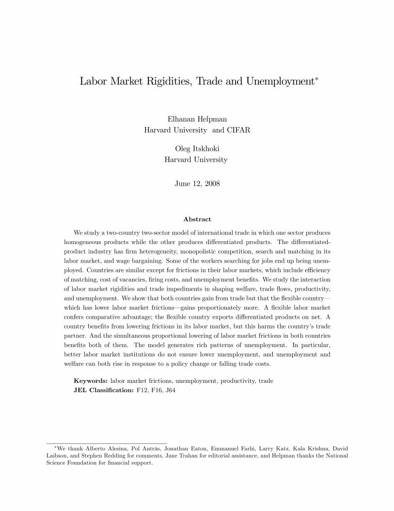
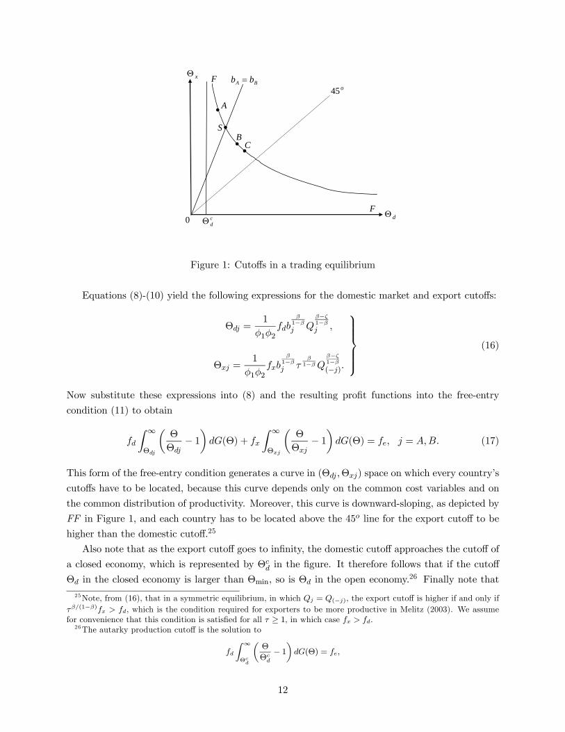
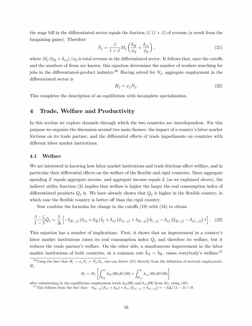
Figure 1: Cutoffs in a trading equilibrium

Equations (8)-(10) yield the following expressions for the domestic market and export cutoffs:

Θdj =1

φ1φ2fdb

β1−βj Q

β−ζ1−βj ,

Θxj =1

φ1φ2fxb

β1−βj τ

β1−βQ

β−ζ1−β(−j).

⎫⎪⎪⎪⎪⎬⎪⎪⎪⎪⎭ (16)

Now substitute these expressions into (8) and the resulting profit functions into the free-entry

condition (11) to obtain

fd

Z ∞

Θdj

µΘ

Θdj− 1¶dG(Θ) + fx

Z ∞

Θxj

µΘ

Θxj− 1¶dG(Θ) = fe, j = A,B. (17)

This form of the free-entry condition generates a curve in (Θdj ,Θxj) space on which every country’s

cutoffs have to be located, because this curve depends only on the common cost variables and on

the common distribution of productivity. Moreover, this curve is downward-sloping, as depicted by

FF in Figure 1, and each country has to be located above the 45o line for the export cutoff to be

higher than the domestic cutoff.25

Also note that as the export cutoff goes to infinity, the domestic cutoff approaches the cutoff of

a closed economy, which is represented by Θcd in the figure. It therefore follows that if the cutoff

Θd in the closed economy is larger than Θmin, so is Θd in the open economy.26 Finally note that

25Note, from (16), that in a symmetric equilibrium, in which Qj = Q(−j), the export cutoff is higher if and only ifτβ/(1−β)fx > fd, which is the condition required for exporters to be more productive in Melitz (2003). We assumefor convenience that this condition is satisfied for all τ ≥ 1, in which case fx > fd.26The autarky production cutoff is the solution to

fd∞

Θcd

Θ

Θcd

− 1 dG(Θ) = fe,

12

(16) yields

Θxj

Θd(−j)=

fxτβ

1−β

fd

∙bj

b(−j)

¸ β1−β

, j = A,B. (18)

Equations (17) and (18) can be used for solving the four cutoffs as functions of labor market frictions

and cost parameters. As is evident, the cutoffs do not depend on the levels of labor market rigidities,

only on their relative size. And once the cutoffs have been solved, they can be substituted into (16)

to obtain solutions for the real consumption indexes Qj .

Our primary interest is in the influence of τ , bA, and bB on the trading economies. We therefore

use (17) and (18) to calculate the impact of these variables on the cutoffs, obtaining

Θdj =δxj∆

h−¡δx(−j) + δd(−j)

¢ ³bj − b(−j)

´−¡δd(−j) − δx(−j)

¢τi,

Θxj =δdj∆

h¡δx(−j) + δd(−j)

¢ ³bj − b(−j)

´+¡δd(−j) − δx(−j)

¢τi,

⎫⎪⎪⎪⎬⎪⎪⎪⎭ (19)

where

δdj =fdΘdj

∞ZΘdj

ΘdG (Θ) , δxj =fxΘxj

∞ZΘxj

ΘdG (Θ) , ∆ =1− β

β(δdAδdB − δxAδxB) .

Note that δdj/φ2 is average revenue per entering firm from domestic sales in country j and δxj/φ2 is

average revenue per entering firm from export sales.27 Moreover, δdj equals average gross operating

profits (not accounting for fixed costs) per entering firm from domestic sales and δxj equals average

gross operating profits per entering firm from exporting.

It is straightforward to show that ∆ > 0.28 Therefore an increase in a country’s relative labor

market frictions, say bj/b(−j), raises the country’s export cutoff and reduces its domestic cutoff, in

addition to reducing the foreign country’s export cutoff and raising the foreign country’s domestic

cutoff. This establishes

Lemma 1 Let bA > bB. Then ΘdA < ΘdB and ΘxA > ΘxB.

Moreover, an increase in country j’s trade cost raises its export cutoff and reduces its domestic

which does not depend on labor market frictions. Note also that Θcd > Θmin if and only if Θ/Θmin > 1 + fe/fd,

where Θ is the mean of Θ, which we assume to be satisfied. This results from the fact that the integral on the left-handside of the above equation is decreasing in Θc

d and assumes its largest value of Θ/Θmin − 1 when Θcd = Θmin.

27To see this, note that profit maximization (5) implies πzj(Θ) = φ2Rzj(Θ) − fz for z = d, x, where Rdj(Θ) isrevenue from domestic sales and Rxj(Θ) is revenue from foreign sales. Then, from the zero profit conditions (9)-(10),we have Rzj(Θ) = fz/φ2 ·Θ/Θzj . As a result, the average revenue per entering firm equals

∞

Θzj

Rzj(Θ)dG(Θ) =fz

φ2Θzj

∞

Θzj

ΘdG(Θ) =δzjφ2

.

28 Proof: To show that ∆ > 0, observe that Θxj > Θdj implies δdj/δxj > (fd/Θdj) / (fx/Θxj) for j = A,B. Usingthese inequalities together with (18) then implies δdAδdB/ (δxAδxB) > τ2β/(1−β) > 1, in which case ∆ > 0. Alsonote that δdAδdB/ (δxAδxB) > τ2β/(1−β) > 1 implies δdj > δxj in at least one country, and that δdj > δxj is alwayssatisfied for both countries in a symmetric equilibrium with bA = bB and hence by continuity in its vicinity.

13

cutoff if and only if δd(−j) > δx(−j). We will shortly show that, indeed, δdj > δxj in both countries

in this type of equilibrium. Therefore an increase in τ raises the export cutoff and reduces the

domestic cutoff in both countries.

These insights can be conveniently summarized with the aid of Figure 1. When the two countries

have the same labor market rigidities, i.e., bA = bB, both have cutoffs at point S in the figure,

which is the intersection of ray bA = bB with FF.29 If, instead, country A has worse labor market

institutions, then A’s cutoffs are at point A while B’s cutoffs are at point B.30 The larger the gap

in labor market frictions between these countries, the higher A is on the FF curve and the lower

B is. In contrast, improvements in the trading environment, which reduce τ , shift down points A

and B along the FF curve. These results have important implications for the variation of outcome

variables across countries, as well as for the international transmission of shocks, which we discuss

below. One immediate implication is that Qj is higher in the flexible country.31 Therefore we state:

Lemma 2 Let bA > bB. Then QA < QB.

For our equations to describe an equilibrium with incomplete specialization, it is necessary

to ensure positive entry of firms in both countries, i.e., Mj > 0 for j = A,B, where Mj is the

number of firms that enter the differentiated sector in country j. This places restrictions on the

permissible difference across countries in labor market rigidities. We now derive implications of

these restrictions.

First, recall that Qζj = PjQj is total spending on differentiated products in country j, and

Mjδzj/φ2 is total revenue from domestic sales when z = d and from foreign sales when z = x.

Since aggregate spending has to equal aggregate revenue, we have32

Qζj =Mj

δdjφ2+M(−j)

δx(−j)φ2

.

Having solved for the cutoffs, which uniquely determine the δzjs, and the real consumption indexes,

29The equation of this ray is derived from (16) to be Θx = τβ/(1−β)fx/fd Θd. Therefore its slope is

τβ/(1−β)fx/fd > 1.30As a convention, we choose country A to be the rigid country and B to be the flexible country.31Proof: Equation (16) implies (QA/QB)

(β−ζ)/(1−β) = (ΘdA/ΘdB) (bB/bA)β/(1−β). It follows that if, say, B is the

flexible country, then bB/bA < 1, and from the previous analysis, ΘdA/ΘdB < 1. As a result, QA/QB < 1.32Alternatively, this condition can be derived from (1), the definition of the real consumption index Qj . A Θ-firm

produces an output level qdj (Θ) = Θ(1−β)/βhdj (Θ) for domestic sales when Θ ≥ Θdj and an output level qxj (Θ) =Θ(1−β)/βhxj (Θ) for export when Θ ≥ Θxj . Foreign buyers consume only qxj (Θ) /τ units of these exportables due tothe variable trade costs. Therefore, if a measure Mj of firms have entered the industry in country j, then

Qj = Mj

∞

Θdj

Θ1−βhdj (Θ)β dG (Θ) +M(−j)τ

−β∞

Θx(−j)

Θ1−βhx(−j) (Θ)

β dG (Θ)

1β

.

Substituting in the equilibrium values of hdj(Θ) and hxj(Θ) from (6) and using (16), yields the equation in the maintext.

14

Qj , these equations yield the following solution for the number of entrants:

Mj =(1− β)φ2

β∆

hδd(−j)Q

ζj − δx(−j)Q

ζ(−j)

i. (20)

It is straightforward to show that δdA > δxA in the rigid country A.33 Under these circumstances

(20) implies MB > 0, because Qj is larger in the flexible country (see Lemma 2). In addition, (20)

implies that a necessary condition for MA > 0 is δdB/δxB > (QB/QA)ζ > 1. In other words, in an

incomplete specialization equilibrium we have δdj > δxj for j = A,B. Moreover, Lemma 1 implies

that δdj is smaller in the flexible country and δxj is larger in the flexible country. We therefore have

Lemma 3 In an equilibrium with incomplete specialization, δdj > δxj in both countries. Moreover,

if bA > bB, then δdA > δdB and δxA < δxB.

This lemma implies that revenues from domestic sales exceeds revenue from exporting, and that

revenue from exporting as a share of total revenue is larger in the flexible country.

Equation (20) can also be used to calculate the difference in entry. In particular,

MA −MB =(1− β)φ2

β∆

h(δdB + δxA)Q

ζA − (δdA + δxB)Q

ζB

i.

Therefore, we have34

Lemma 4 Let bA > bB. Then MA < MB.

We show in the Appendix that for every τ > 1 there exists a unique threshold b (τ) > 1, such

that Mj > 0 for j = A,B if and only if bA/bB < b (τ), where A is the rigid country. When

bA/bB ≥ b (τ), the rigid country specializes in homogeneous goods. Evidently, b (τ) provides an

upper bound on differences in labor market frictions that support equilibria with production of

differentiated products in both countries.35

Next consider the determinants of the number of workers searching for jobs in the differentiated

sector, Nj , and aggregate employment in that sector, Hj . On the one hand, the wage bill in the

differentiated sector, wjHj , equals Nj , because the wage rate is wj = bj = 1/xj (see (14)) and

xj = Hj/Nj by definition. This implies that aggregate income equals L, where Nj is derived from

the differentiated sector and L−Nj is derived from the homogeneous sector. On the other hand,

33Since ∆ > 0, it is necessary to have δdj > δxj in at least one country. However, the rigid country A has ahigher export cutoff and a lower domestic cutoff. Therefore δdA > δxA in the rigid country. Moreover, as shown infootnote 28, δdB > δxB in the flexible country as well, as long as labor market rigidities do not differ much acrosscountries.34Proof: Let B be the flexible country. Then from Lemmas 2 and 3, δdB < δdA, δxA < δxB, and QB > QA, in

which case MB > MA.35Given τ , this limit can be depicted by point C on the FF curve in Figure 1, which is located between the

bA = bB ray and the 45o line, such that the equilibrium point of the flexible country, point B, has to be above C forboth countries to be incompletely specialized. In the Appendix we also analyze equilibria with specialization whenbA/bB ≥ b(τ).

15

the wage bill in the differentiated sector equals the fraction β/ (1 + β) of revenue (a result from the

bargaining game). Therefore

Nj =β

1 + βMj

µδdjφ2+

δxjφ2

¶, (21)

whereMj (δdj + δxj) /φ2 is total revenue in the differentiated sector. It follows that, once the cutoffs

and the numbers of firms are known, this equation determines the number of workers searching for

jobs in the differentiated-product industry.36 Having solved for Nj , aggregate employment in the

differentiated sector is

Hj = xjNj . (22)

This completes the description of an equilibrium with incomplete specialization.

4 Trade, Welfare and Productivity

In this section we explore channels through which the two countries are interdependent. For this

purpose we organize the discussion around two main themes: the impact of a country’s labor market

frictions on its trade partner, and the differential effects of trade impediments on countries with

different labor market institutions.

4.1 Welfare

We are interested in knowing how labor market institutions and trade frictions affect welfare, and in

particular their differential effects on the welfare of the flexible and rigid countries. Since aggregate

spending E equals aggregate income, and aggregate income equals L (as we explained above), the

indirect utility function (3) implies that welfare is higher the larger the real consumption index of

differentiated products Qj is. We have already shown that Qj is higher in the flexible country, in

which case the flexible country is better off than the rigid country.

Now combine the formulas for change in the cutoffs (19) with (16) to obtain

β − ζ

1− βQj =

1

∆

h−δd(−j) (δxj + δdj) bj + δxj

¡δx(−j) + δd(−j)

¢b(−j) − δxj

¡δd(−j) − δx(−j)

¢τi. (23)

This equation has a number of implications. First, it shows that an improvement in a country’s

labor market institutions raises its real consumption index Qj and therefore its welfare, but it

reduces the trade partner’s welfare. On the other side, a simultaneous improvement in the labor

market institutions of both countries, at a common rate bA = bB, raises everybody’s welfare.37

36Using the fact that Hj = xjNj = Nj/bj , one can derive (21) directly from the definition of sectoral employment,Hj :

Hj =Mj

∞

Θdj

hdj (Θ) dG (Θ) +∞

Θxj

hxj (Θ) dG (Θ) ,

after substituting in the equilibrium employment levels hdj(Θ) and hxj(Θ) from (6), using (16).37This follows from the fact that −δd(−j) (δxj + δdj) + δxj δx(−j) + δd(−j) = −β∆/ (1− β) < 0.

16

Second, in view of Lemma 3 (specifically, in view of δdj > δxj in both countries), a reduction in

trade impediments raises welfare in both countries. We summarize these findings in38

Proposition 1 (i) Welfare is higher in the flexible country. (ii) An improvement in labor marketinstitutions in one country raises its welfare and reduces the welfare of its trade partner. (iii) A si-

multaneous improvement in labor market institutions in both countries, with bA = bB, raises welfare

in both of them. (iv) A reduction of trade impediments raises welfare in both countries and Qj rises

proportionately more in the flexible country.

The second part of this proposition is intriguing: it states that a country harms the trade partner

by improving its own labor market institutions. Moreover, this happens despite the fact that the

trade partner (−j) enjoys better terms of trade as a result of improved labor market institutions incountry j, because (−j) pays lower prices for imported varieties from j. The reason for this result is

that better labor market institution in country j act like productivity improvements in this country,

which makes foreign firms less competitive and therefore crowds them out from the differentiated

sector. As a result, fewer foreign firms enter the industry, which harms foreign welfare, and this

negative welfare effect is larger than the welfare gain from improved terms of trade.39

Proposition 1 also establishes that the gains from trade are unequally distributed, with the

flexible country gaining more. The reason is that, before trade liberalization, the differentiated-

product market is more competitive in the flexible country than in the rigid country (i.e., P is lower

in the flexible country). As a result, exporters of brands of the differentiated product gain from

foreign-market access more in the flexible country than in the rigid country.40

The last part of this proposition establishes that both countries gain from trade, because autarky

is attained when τ → ∞.41 Moreover, we show in the Appendix that both countries gain from

trade when the difference in labor market institutions is large enough to effect an equilibrium in

which the rigid country specializes in the production of homogeneous products. We therefore have

Proposition 2 Both countries gain from trade.38The very last part of the proposition follows from the fact that (23) implies

β − ζ

1− βQj − Q(−j) = − 1

∆(δdj + δxj) δd(−j) + δx(−j) bj − b(−j) + δd(−j)δxj − δx(−j)δdj τ .

Under these circumstances Qj > Q(−j) in response to τ < 0, when bj < b(−j) (by Lemma 3) .39Demidova (2006) studies a full employment model with exogenous differences in productivity distributions across

countries, and finds that: (a) productivity improvements in one country hurt its trade partner; and (b) fallingtrade costs benefit disproportionately the more productive country, and may even hurt the less productive country.Our results on labor market frictions are similar to these (except that in our case both countries necessarily gainfrom falling trade costs), because–not withstanding unemployment–labor market frictions have analogous effectsto productivity.40Additional intuition is obtained from Lemma 3, which implies that firms in the flexible country receive a larger

fraction of revenue from exporting. As a result, falling trade costs result in a larger increase in profitability ofexporting firms in the flexible country, which leads to relatively more entry in this country and to disproportionatelyhigher welfare gains.41The following is a direct proof of the gains-from-trade argument: We have seen that the domestic cutoff is higher

in every country in the trading equilibrium than in autarky. The first equation in (16) then implies that Qj is higherin every country in the trading equilibrium, because this equation also holds in autarky.

17

This proposition is interesting, because it is well known that gains from trade are not ensured in

economies with nonconvexities and distortions.42 Moreover, in addition to the standard nonconvex-

ities and distortions that exist in models of monopolistic competition, our model contains frictions

in labor markets, which makes the gains-from-trade result even more remarkable.

4.2 Trade Structure

From Lemma 1 we know that the country with better labor market institutions has a lower export

cutoff and a higher domestic cutoff; therefore it also has a larger fraction of exporting firms in the

differentiated-product sector. In addition, we know that exports per entering firm equal δxj/φ2.

Therefore exports of differentiated products from country j to (−j) are

Xj =Mjδxjφ2

.

Lemma 3 states that the country with better labor market institutions has a larger δxj and Lemma 4

states that it has more firms. Therefore the flexible country exports a higher value of differentiated

products Xj , which implies that it exports differentiated products on net. As a consequence, the

rigid country exports homogeneous goods.

As in the standard Helpman-Krugman model of trade in differentiated products, there is intra-

industry trade. We can therefore decompose the volume of trade into intra-industry and intersec-

toral trade. Let country A be the rigid country and let B be the flexible country. Then, because

trade is balanced, the total volume of trade equals 2XB and the volume of intra-industry trade

equals 2XA. Therefore the share of intra-industry trade equals

XA

XB=

δxAMA

δxBMB.

Using (20) this share can be expressed as

XA

XB=

δdBδxB−µQB

QA

¶ζ

δdAδxA

µQB

QA

¶ζ

− 1.

Equations (19) and (23) then imply that the share of intra-industry trade is smaller the larger the

ratio bA/bB is.

The results on trade structure are summarized in

Proposition 3 (i) A larger fraction of firms export in the flexible country. (ii) The flexible countryexports differentiated products on net and imports homogeneous goods. (iii) The share of intra-

industry trade is smaller the larger the proportional gap in labor market institutions.

42See Helpman and Krugman (1985).

18

That is, labor market institutions impact comparative advantage and the share of intra-industry

trade in a particular way. Evidently, these are testable implications about trade flows.43

4.3 Productivity

In this section we discuss the implications of our model for total factor productivity (TFP). Al-

ternative measures of TFP can be used to characterize the efficiency of production. We choose to

focus on one such measure–the employment-weighted average of firm-level productivity–which is

commonly used in the literature.44 In the differentiated-product sector this measure is

TFP j =Mj

Hj

"Z ∞

Θdj

Θ1−ββ hdj(Θ)dG(Θ) +

Z ∞

Θxj

Θ1−ββ hxj(Θ)dG(Θ)

#. (24)

Recall that qzj(Θ) = Θ(1−β)/βhzj(Θ) for z = d, x. Therefore, TFP j equals the output of differ-

entiated products divided by employment in the differentiated-product sector.45 Note that TFP j

measures productivity in the differentiated-product sector only, rather than in the entire economy,

and productivity in the homogeneous-product sector is constant and equal to one. We discuss in

the Appendix a productivity measure that accounts for the compositional effects across sectors.

Using (6) and (8)-(10), we can express (24) as

TFP j =δdjϕdj + δxjϕxj

δdj + δxj= djϕdj + xjϕxj , (25)

where dj = δdj/(δdj+δxj) is the share of domestic sales in revenue and xj is the share of exports,

i.e., xj = 1− dj , j = A,B. Moreover,

ϕzj ≡ ϕ(Θzj) =

R∞ΘzjΘ1/βdG(Θ)R∞

ΘzjΘdG(Θ)

, z = d, x,

where ϕdj represents the average productivity of firms that serve the home market and ϕxj repre-

sents the average productivity of exporting firms. It follows that aggregate productivity equals the

weighted average of the productivity of firms that serve the domestic market and the productivity

of firms that export, with the revenue shares serving as weights. We show in the Appendix that ϕ(·)is an increasing function. Therefore average productivity is higher among exporters, i.e., ϕxj > ϕdj .

Expression (25) implies that the cutoffs Θdj ,Θxj uniquely determine the TFP js, because zj

43Additionally, under Pareto-distributed productivity, the model also implies that the volume of trade is larger thelarger the gap in labor market rigidities is and the smaller the trade impediments are (see Appendix).44This corresponds to the measure analyzed by Melitz (2003) in the appendix. Note that Melitz uses revenue to

weight firm productivity levels. However, in equilibrium, revenue is proportional to employment, in which case hisand our productivity indexes are the same.45An alternative, and potentially more desirable, measure of productivity, would divide output by the number of

workers searching for jobs in the differentiated-product sector, Nj . This measure is always smaller than TFPj by thefactor xj . It follows that labor market liberalization has an additional positive effect on this measure of productivityas compared to the measure used in the main text.

19

and ϕzj depend only on the cutoffs. Moreover, since the two cutoffs are linked by the free-entry

condition (17), TFP j can be expressed as a function of the domestic cutoff Θdj . This implies that

in a closed economy TFP j is not responsive to changes in labor market institutions, because Θcd

is uniquely determined by the fixed costs of entry and production and the ex ante productivity

distribution.

Productivity TFP j is higher in the trade equilibrium than in autarky, because ϕ(Θxj) >

ϕ(Θdj) > ϕ(Θcd), and in autarky

cx = 0. That is, the average productivity of exporters and

nonexporters alike is higher in the trade equilibrium than is the average productivity of firms in

autarky. In addition, trade reallocates revenue to the exporting firms, which are on average more

productive. For both these reasons trade raises TFP j . We summarize these results in

Proposition 4 (i) In the closed economy, TFPj does not depend on the quality of labor marketinstitutions; (ii) TFPj is higher in any trade equilibrium than in autarky.

Next recall that in an open economy a reduction of trade costs raises the domestic cutoff and

reduces the export cutoff. In addition, an improvement in labor market institutions in country

j raises Θdj and Θx(−j) and reduces Θd(−j) and Θxj . Finally, a simultaneous and proportional

improvement in labor market institutions in both countries (i.e., bA = bB < 0) leaves all these

cutoffs unchanged (see (19)).

How do changes in labor market frictions impact productivity? In the case in which both coun-

tries’ labor market frictions decline by the same factor of proportionality, the answer is simple: the

TFP js do not change. As long as productivity is measured with regard to the number of employed

workers rather than the number of workers searching for jobs, measured sectoral productivity levels

are not sensitive to the absolute level of frictions in the labor markets; only the relative level of

these frictions matters. This result points to a shortcoming of this TFP measure. We nevertheless

continue the analysis with this measure, because it is commonly used in the literature.

A shock that raises the domestic cutoff Θdj and reduces the export cutoff Θxj affects TFP j

through three channels. First, the reallocation of revenue from firms that serve the home market

to exporters raises the weight on the productivity of exporters, xj , which raises in turn TFPj .

Second, some least-efficient firms exit the industry, thereby raising the average productivity of firms

that sell only in the home market, ϕdj , which raises TFP j . Finally, some firms with productivity

below Θxj begin to export, thereby reducing the average productivity of exporters, ϕxj , which

reduces TFPj .46

The presence of the third effect, which goes against the first two, does not enable us to sign

the impact of single-country labor market reforms on productivity; in general, productivity may

increase or decrease. The sharp result for the comparison of autarky to trade derives from the

fact that, in a move from autarky to trade, the third effect is nil. In the Appendix, we provide

sufficient conditions for productivity to be monotonically rising with Θdj , and therefore declining

46Formally, this decomposition can be represented as [TFP j = ˆ xj(ϕxj−ϕdj)+(1− xj)ϕdj+ xjϕxj with ˆ xj > 0,ϕdj > 0 and ϕxj < 0.

20

with bj and τ and rising with b(−j). In this section, however, we limit our discussion to the case of

Pareto-distributed productivity draws, which yields sharp predictions.

Under the assumption of Pareto-distributed productivity, that is, G (Θ) = 1 − (Θmin/Θ)k forΘ ≥ Θmin, (25) yields47

[TFP j =δdj¡ϕxj − ϕdj

¢ ³k − 1−β

β

´δdjϕdj + δxjϕxj

Θdj , (26)

where k > 1/β is required for TFP j to be finite, and we therefore assume that it holds. As a result,

TFP j is higher the higher Θdj is (and the lower Θxj is). It follows that productivity is higher in the

flexible country, and an improvement in a country’s labor market institutions raises its productivity

and reduces the productivity of its trade partner. An implication of this result is that the gap in

productivity between the flexible and rigid countries is increasing in bA/bB, the relative quality of

their labor market institutions. These results are summarized in

Proposition 5 Let Θ be Pareto-distributed with a shape parameter k > 1/β. Then: (i) TFPj is

higher in the flexible country; (ii) an improvement in labor market institutions in country j raises

TFPj and reduces TFP(−j); (iii) a reduction of trade costs raises TFPj in both countries.

In other words, total factor productivity is higher in the flexible country, and while a reduction of

labor market frictions in any country raises its own total factor productivity, this hurts the total

factor productivity of the country’s trade partner.

5 Unemployment

Before discussing the variation of unemployment across countries with different labor market insti-

tutions in Sections 5.2 and 5.3, we first examine the determinants of unemployment in a world of

symmetric countries.

5.1 Symmetric Countries

We study in this section countries with bA = bB = b, in order to understand how changes in

the common level of labor market frictions and the common level of variable trade costs affect

unemployment. In such equilibria, the cutoffs Θd and Θx, the consumption index Q, the number

of entrants M , the number of individuals searching for jobs in the differentiated-product sector N ,

the number of workers employed in that sector H, and the rate of unemployment u are the same

in both countries. We therefore drop the country index j for convenience. From Section 3 we know

that two symmetric economies are at the same point on the FF curve in Figure 1 (point S), the

location of this point is invariant to the common level of labor market frictions, and this point is

higher the larger τ is. Moreover, (23) implies that Q is lower the higher are either b or τ , and a

47 In this calculation, an increase in Θdj is accompanied by a decrease in Θxj in order to satisfy the free-entrycondition (17). See Appendix for derivation of this equation.

21

0b

u

1

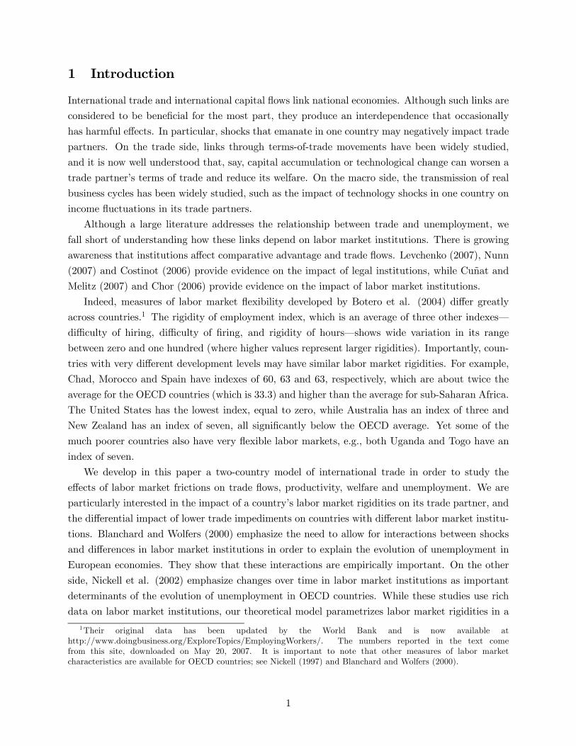
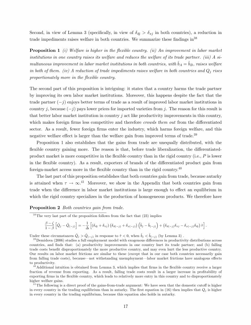
Figure 2: Unemployment in a world of symmetric countries

lower value of Q leads to lower welfare. In other words, higher frictions in trade or labor markets

reduce welfare.

In order to assess the impact of labor market rigidities on unemployment, we need to know

their quantitative impact on Q. For this reason we use (23) to obtain

Q = − β

β − ζ

µb+

δxδd + δx

τ

¶.

Next combine (20) and (21) to obtain N = βQζ/ (1 + β), which together with the previous equation

yields

N = − βζ

β − ζ

µb+

δxδd + δx

τ

¶.

Finally, from (14) and the unemployment equation (15), we have u = N+ b/ (b− 1), which togetherwith the formula for N implies

u =

µ1

b− 1 −βζ

β − ζ

¶b− βζ

β − ζ

δxδd + δx

τ .

It is evident from this formula that better labor market institutions (lower b) reduce unemployment

if and only if

b < 1 +β − ζ

βζ,

i.e., if and only if labor market frictions are low to begin with. If these frictions are high, however,

and the above inequality is reversed, then improvements in labor market institutions raise the rate of

unemployment. In fact, the relationship between b and the rate of unemployment has an inverted U

shape as depicted in Figure 2. To understand this result, note that changes in labor market frictions

impact unemployment through two channels: the rate of unemployment in the differentiated sector

22

1−x, and the fraction of people searching for jobs in this sector N/L. Improvements in labor market

institutions raise x and thereby reduce the rate of unemployment. On the other hand, improvements

in labor market institutions attract more workers to the differentiated-product sector and thereby

raise the rate of unemployment. The former dominates when labor market frictions are low, while

the latter dominates when labor market frictions are high.48

Now consider changes in trade impediments. As the formula for change in the rate of unemploy-

ment shows, a lower trade cost τ raises the rate of unemployment, independently of the common

level of frictions in labor markets or the initial level of trade frictions.49 Since the lowering of trade

costs raises welfare, this means that welfare and unemployment respond in opposite directions to

changes in trade costs. And since reducing trade impediments does not affect tightness in labor

markets, the rise in unemployment is a consequence of an increase in N and H by the same factor

of proportionality.

We summarize the main findings of this section in

Proposition 6 In a symmetric world economy: (i) improvements in labor market institutions,common to both countries, reduce unemployment if and only if frictions in the labor markets are

low and satisfy b < 1 + (β − ζ) /βζ; and (ii) reductions in trade impediments raise unemployment.

An intriguing result is that lower trade barriers raise unemployment. To understand the intuition

behind this result, observe that the lowering of trade impediments makes exporting more profitable

in the differentiated-product sector, without affecting tightness in its labor market. As a result,

more firms choose to export in this industry and exporters choose to export larger volumes. In

addition, domestic firms that do not serve foreign markets become less profitable, which leads

to more exit of low-productivity firms. On account of these changes labor demand rises. To

accommodate this demand, more individuals search for jobs in the differentiated-product industry.

Under these circumstances, the sectoral unemployment rates remain the same, but the economy’s

unemployment rises because more workers choose to attach themselves to the high-wage sector,

which has the higher rate of unemployment.

Also note that unemployment can increase or decrease when welfare rises. That is, depending

on the nature of the disturbance and the initial institutional environment, unemployment and

welfare can move in the same or in opposite directions. For this reason changes in unemployment

do not reflect changes in welfare. This results from the standard property of search and matching

models, in which unemployment is a productive activity; it enables workers to be employed in both

low-wage and high-wage activities. Under these circumstances an expansion of the high-wage\high-unemployment sector results in higher unemployment, but may also raise welfare. In this type of

environment, other statistics–such as total employment in the high-wage sector H–better proxy

for welfare than the rate of unemployment.

48 It can also be shown that in the symmetric case lower frictions in labor markets lead to increased entry of firmsM , an increase in N proportionately to M , and a more than proportional increase in employment H.49The effect of a reduction in trade costs on unemployment is larger the larger is the share of trade in the sector’s

revenue, i.e., the larger is δxj/ (δdj + δxj). When the economies are nearly closed, this effect is very small.

23

5.2 Small Asymmetries

Consider a world in which country B has the better labor market institutions, so that bA > bB.

Then the labor market is tighter in the flexible country B, and the unemployment rate is lower in

its differentiated-product sector. The question is whether the country’s overall unemployment rate

is also lower? The reason this may not be the case is that more individuals might be searching for

jobs in the high-unemployment sector in the country with lower labor market frictions. We answer

this question below for the case in which labor rigidities do not vary much across countries. In the

next section we discuss global comparisons for the case in which productivity is distributed Pareto.

Suppose that we start from a symmetric equilibrium with bA = bB. As a result, the two

countries look alike in all respects. Next suppose that labor market rigidities rise in country A

but do not change in country B, so that bA > 0 and bB = 0. Then we can use (19) and (23) to

calculate the response of the cutoffs and the real consumption index in each of these countries,

evaluated at the initially symmetric equilibrium, and we can combine these results with the other

equilibrium conditions to derive the proportional change in the number of individuals seeking jobs

in the differentiated-product sectors of both countries. The technical details are provided in the

Appendix, where we show that

NA = −ΨNA bA,

NB = ΨNB bA,

where the coefficients ΨNj are determined by the initial equilibrium, ΨNA > βζ/(β − ζ), ΨNB > 0,

and where ΨNA → βζ/(β − ζ) and ΨNB → 0 as τ → ∞. Evidently, an increase in labor marketfrictions in country A reduces the number of individuals searching for jobs in A’s differentiated-

product sector and increases the number of individuals searching for jobs in country B. Under

these circumstances, (15) yields

uA = −µΨNA −

1

b− 1

¶bA,

uB = ΨNB bA.

The implication is that the deterioration of labor market institutions in A raises unemployment in

B, while unemployment rises in A if and only if b < 1 + 1/ΨNA, i.e., if and only if the frictions

in the labor markets are low to begin with; otherwise the rate of unemployment declines in A.

Since ΨNA > βζ/(β − ζ), the open economy A would require even lower labor market frictions

than a comparable closed economy for a deterioration in its labor market institutions to raise its

unemployment. Moreover, since

uA − uB = −µΨNA +ΨNB −

1

b− 1

¶bA,

country A has the higher rate of unemployment after a deterioration in its labor market institutions

24

if and only if

b < 1 +1

ΨNA +ΨNB,

or if and only if the initial level of frictions in the labor market is rather low. If the initial level

of frictions in the labor markets is high, thereby violating this inequality, then country A has the

lower rate of unemployment.

These results are summarized in

Proposition 7 In the vicinity of a symmetric equilibrium: (i) the flexible country has a lower rateof unemployment if and only if the level of friction in both labor markets are low, i.e., if and only if

b < 1 + 1/ (ΨNA +ΨNB); and (ii) an improvement in a country’s labor market institutions reduces

the rate of unemployment in its trade partner, yet it reduces home unemployment if and only if the

initial level of friction in both labor markets are low, i.e., if and only if b < 1 + 1/ΨNA.

It is evident from this proposition that a country’s level of unemployment depends not only on its

own labor market institutions but also on those of its trade partner. Moreover, better domestic

labor market institutions do not guarantee lower unemployment relative to the trade partner, unless

the frictions in both labor markets are low. As a result, one cannot infer differences in labor market

institutions from observations of unemployment rates.

To understand the intuition behind these results, first note that an improvement in a country’s

labor market institutions affects its unemployment rate through two channels: on the one hand, the

country’s labor market becomes tighter, which reduces the unemployment rate in its differentiated-

product sector; on the other hand, more workers search for jobs in the differentiated-product

sector. As a result of these opposing effects, the overall rate of unemployment declines when the

first channel dominates and rises when the second channel dominates. The first channel dominates

when the frictions in the labor markets are small, while the second channel dominates when these

frictions are large.

An interesting implication of Proposition 7 is that improvements in a country’s labor market

institutions reduces the rate of unemployment in its trade partner. This results from the fact

that a reduction of frictions in the labor market of country j makes j more competitive in the

differentiated-product industry. As a result, the demand shifts from brands of country (−j) tobrands of j. In response, the differentiated-product sector contracts in country (−j), which meansthat fewer people search there for jobs in this industry. Since the labor market frictions do not

change in country (−j), the rate of unemployment in its differentiated-product sector does notchange either. It therefore follows that the overall rate of unemployment declines in (−j) becausefewer workers search there for jobs and the fraction of those who find employment does not change.

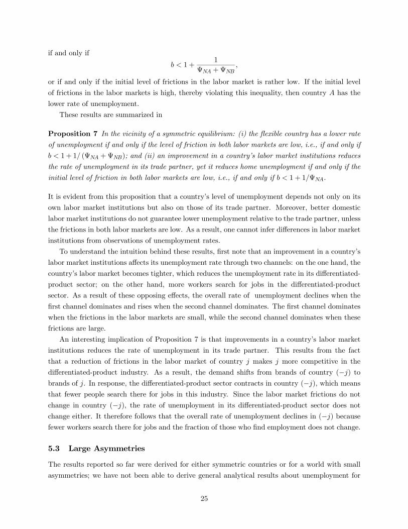
5.3 Large Asymmetries

The results reported so far were derived for either symmetric countries or for a world with small

asymmetries; we have not been able to derive general analytical results about unemployment for

25

countries with large differences in labor market rigidities. To make progress on this issue, we

therefore turn to the case of Pareto-distributed productivity levels, and after deriving one analytical

result we resort to simulations. The following numerical examples are interesting, because they show

how unemployment rates compare across countries when labor frictions differ substantially across

countries, and they show how the degree of similarity in labor market institutions interacts with

trade frictions in shaping unemployment rates.

For the purpose of the simulations we assume that productivity is distributed Pareto. Therefore

the distribution function is

G (Θ) = 1−µΘminΘ

¶k

, for Θ ≥ Θmin and k > 2.

As is well known, the shape parameter k controls the dispersion of Θ, with smaller values of k

representing more dispersion. It has to be larger than two for the variance of productivity to be

finite. We show in the Appendix how the equilibrium conditions are simplified when productivity

is distributed Pareto, and these equations are used to generate our numerical examples. One

convenient implication of the Pareto assumption is that condition (11) implies δdj + δxj = kfe, and

therefore aggregate revenue in the differentiated sector is independent of labor market frictions and

is the same in both countries.

Combining (20) and (21), we obtain the following expression for global revenues generated in

the differentiated sector:

QζA +Qζ

B =1

φ2

£MA(δdA + δxA) +MB(δdB + δxB)

¤=1 + β

β(NA +NB).

Therefore, whenever QζA+Q

ζB rises, the world-wide allocation of workers to the differentiated sector,

NA +NB, must also increase. Moreover, under the Pareto assumption

QζA +Qζ

B =kfeφ2(MA +MB),

so that the total number of entrants into the differentiated sector must also increase. Finally, under

the Pareto assumption equation (21) implies

Nj

Mj=

β

1− βkfe.

That is, the number of workers searching for jobs in the differentiated sector relative to the number

of firms is the same in both countries and independent of trade or labor market frictions.

Next note that Proposition 1 establishes that a reduction in trade costs raises Qj in both

countries. Therefore, the above discussion implies that a reduction in trade costs increases NA+NB

and MA +MB by the same factor of proportionality. In the Appendix we also show that NA/NB

declines with reductions in τ when A is the rigid country, i.e., bA > bB. This then implies that NB,

the number of job-seekers in the differentiated sector of the flexible country B, necessarily increases.

26

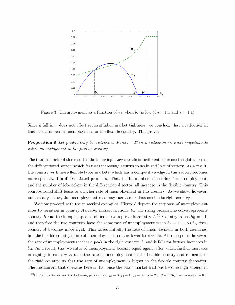
A

1 1.05 1.1 1.15 1.2 1.25 1.3 1.35 1.4 1.450

0.01

0.02

0.03

0.04

0.05

0.06

0.07

0.08

0.09

0.1

Bu

Au

BbAb'b ''b

Figure 3: Unemployment as a function of bA when bB is low (bB = 1.1 and τ = 1.1)

Since a fall in τ does not affect sectoral labor market tightness, we conclude that a reduction in

trade costs increases unemployment in the flexible country. This proves

Proposition 8 Let productivity be distributed Pareto. Then a reduction in trade impediments

raises unemployment in the flexible country.

The intuition behind this result is the following. Lower trade impediments increase the global size of

the differentiated sector, which features increasing returns to scale and love of variety. As a result,

the country with more flexible labor markets, which has a competitive edge in this sector, becomes

more specialized in differentiated products. That is, the number of entering firms, employment,

and the number of job-seekers in the differentiated sector, all increase in the flexible country. This

compositional shift leads to a higher rate of unemployment in this country. As we show, however,

numerically below, the unemployment rate may increase or decrease in the rigid country.

We now proceed with the numerical examples. Figure 3 depicts the response of unemployment

rates to variation in country A’s labor market frictions, bA; the rising broken-line curve represents

country B and the hump-shaped solid-line curve represents country A.50 Country B has bB = 1.1,

and therefore the two countries have the same rate of unemployment when bA = 1.1. As bA rises,

country A becomes more rigid. This raises initially the rate of unemployment in both countries,

but the flexible country’s rate of unemployment remains lower for a while. At some point, however,

the rate of unemployment reaches a peak in the rigid country A, and it falls for further increases in

bA. As a result, the two rates of unemployment become equal again, after which further increases

in rigidity in country A raise the rate of unemployment in the flexible country and reduce it in

the rigid country, so that the rate of unemployment is higher in the flexible country thereafter.

The mechanism that operates here is that once the labor market frictions become high enough in

50 In Figures 3-4 we use the following parameters: fx = 3, fd = 1, fe = 0.5, k = 2.5, β = 0.75, ζ = 0.5 and L = 0.1.

27

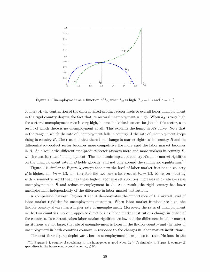
1 1.1 1.2 1.3 1.4 1.5 1.60

0.02

0.04

0.06

0.08

0.1

0.12

0.14

0.16

0.18

0.2

Bu

BbAb'b

Au

ob

Figure 4: Unemployment as a function of bA when bB is high (bB = 1.3 and τ = 1.1)

country A, the contraction of the differentiated-product sector leads to overall lower unemployment

in the rigid country despite the fact that its sectoral unemployment is high. When bA is very high

the sectoral unemployment rate is very high, but no individuals search for jobs in this sector, as a

result of which there is no unemployment at all. This explains the hump in A’s curve. Note that

in the range in which the rate of unemployment falls in country A the rate of unemployment keeps

rising in country B. The reason is that there is no change in market tightness in country B and its

differentiated-product sector becomes more competitive the more rigid the labor market becomes

in A. As a result the differentiated-product sector attracts more and more workers in country B,

which raises its rate of unemployment. The monotonic impact of country A’s labor market rigidities

on the unemployment rate in B holds globally, and not only around the symmetric equilibrium.51

Figure 4 is similar to Figure 3, except that now the level of labor market frictions in country

B is higher, i.e., bB = 1.3, and therefore the two curves intersect at bA = 1.3. Moreover, starting

with a symmetric world that has these higher labor market rigidities, increases in bA always raise

unemployment in B and reduce unemployment in A. As a result, the rigid country has lower

unemployment independently of the difference in labor market institutions.

A comparison between Figures 3 and 4 demonstrates the importance of the overall level of

labor market rigidities for unemployment outcomes. When labor market frictions are high, the

flexible country always has a higher rate of unemployment. Moreover, the rates of unemployment

in the two countries move in opposite directions as labor market institutions change in either of

the countries. In contrast, when labor market rigidities are low and the differences in labor market

institutions are not large, the rate of unemployment is lower in the flexible country and the rates of

unemployment in both countries co-move in response to the changes in labor market institutions.

The next three figures depict variations in unemployment in response to trade frictions, in the51 In Figures 3-4, country A specializes in the homogeneous good when bA ≥ b0; similarly, in Figure 4, country B

specializes in the homogeneous good when bA ≤ bo.

28

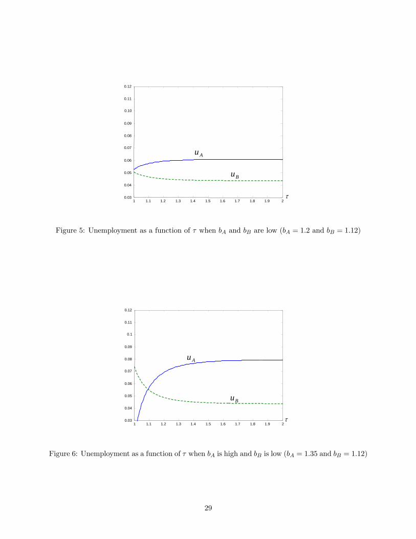
1 1.1 1.2 1.3 1.4 1.5 1.6 1.7 1.8 1.9 20.03

0.04

0.05

0.06

0.07

0.08

0.09

0.10

0.11

0.12

Bu

τ

Au

Figure 5: Unemployment as a function of τ when bA and bB are low (bA = 1.2 and bB = 1.12)

1 1.1 1.2 1.3 1.4 1.5 1.6 1.7 1.8 1.9 20.03

0.04

0.05

0.06

0.07

0.08

0.09

0.1

0.11

0.12

Bu

τ

Au

Figure 6: Unemployment as a function of τ when bA is high and bB is low (bA = 1.35 and bB = 1.12)

29

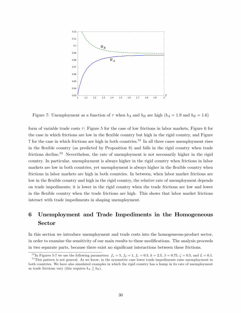
τ1 1.1 1.2 1.3 1.4 1.5 1.6 1.7 1.8 1.9 2

0.03

0.04

0.05

0.06

0.07

0.08

0.09

0.1

0.11

0.12

Bu

Au

Figure 7: Unemployment as a function of τ when bA and bB are high (bA = 1.9 and bB = 1.6)

form of variable trade costs τ : Figure 5 for the case of low frictions in labor markets, Figure 6 for

the case in which frictions are low in the flexible country but high in the rigid country, and Figure

7 for the case in which frictions are high in both countries.52 In all three cases unemployment rises

in the flexible country (as predicted by Proposition 8) and falls in the rigid country when trade

frictions decline.53 Nevertheless, the rate of unemployment is not necessarily higher in the rigid

country. In particular, unemployment is always higher in the rigid country when frictions in labor

markets are low in both countries, yet unemployment is always higher in the flexible country when

frictions in labor markets are high in both countries. In between, when labor market frictions are

low in the flexible country and high in the rigid country, the relative rate of unemployment depends

on trade impediments; it is lower in the rigid country when the trade frictions are low and lower

in the flexible country when the trade frictions are high. This shows that labor market frictions

interact with trade impediments in shaping unemployment.

6 Unemployment and Trade Impediments in the HomogeneousSector

In this section we introduce unemployment and trade costs into the homogeneous-product sector,

in order to examine the sensitivity of our main results to these modifications. The analysis proceeds

in two separate parts, because there exist no significant interactions between these frictions.

52 In Figures 5-7 we use the following parameters: fx = 5, fd = 1, fe = 0.5, k = 2.5, β = 0.75, ζ = 0.5, and L = 0.1.53This pattern is not general. As we know, in the symmetric case lower trade impediments raise unemployment in

both countries. We have also simulated examples in which the rigid country has a hump in its rate of unemploymentas trade frictions vary (this requires bA & bB).

30

6.1 Unemployment in the Homogeneous Sector

To introduce unemployment into the homogeneous-product sector in a simple way, assume as before

that in this sector the product market and the labor market are both competitive, so that output is

sold for p0j = 1 and every employed worker gets the same wage rate w0j = 1. Unlike the previous

case, however, now assume that a worker has a marginal product of one with probability x0j ,

0 < x0j < 1, and zero with probability 1− x0j , and that this information is revealed only after he

attaches himself to the homogeneous sector. If not productive, the worker cannot get a job and he

becomes unemployed. If productive, he gets a job and a wage of one. Under these circumstances

the sectoral unemployment rate in the homogeneous-product industry is 1− x0j .

Except for this modification, all other features of the model remain the same. As a result, the

equilibrium wage rate in the differentiated sector of country j is wj = bj , where bj = ajxαj is the

equilibrium hiring cost and xj is the measure of tightness in the differentiated sector’s labor market.

Since xj also equals the probability of finding a job in the differentiated sector, the indifference

condition for workers between searching for jobs in the two sectors is w0jx0j = wjxj , or x0j = bjxj .

Together with bj = ajxαj this condition implies that

xj =

µx0jaj

¶ 11+α

and bj =¡ajx

α0j

¢ 11+α . (27)

Therefore, as before, xj is decreasing and bj is increasing in aj (see (14)).54 In addition, tightness

in the labor market, xj , and the cost of search and matching, bj , now depend on x0j . In particular,

a higher probability of employment in the homogeneous sector leads to a tighter labor market in

the differentiated sector and to higher hiring costs in that sector. As a result, the wage rate rises

in the differentiated sector.

Having the solution to (bj , xj) from (27), we can next solve for the sectoral allocation of re-

sources, because the equilibrium conditions in the differentiated sector do not change. For example,

the zero-profit condition (16) and the free-entry condition (17) remain the same.55 As a result, all

propositions from Section 4 remain valid. In particular, both countries gain from trade: the rigid

country imports differentiated products on net, and the flexible country has a more productive

differentiated-product sector.

The equilibrium unemployment rate is now given by

uj = (1− x0j)L−Nj

L+ (1− xj)

Nj

L,

where the right-hand side of the equation expresses the rate of unemployment as a weighted average

of sectoral rates of unemployment. This formula emphasizes a new feature: an expansion of the

workforce that searches for jobs in the differentiated sector raises unemployment if and only if the

54To guarantee an interior solution, we now require aj > x0j , which ensures xj < 1. However, this does not implybj > 1 any more.55Note, however, that now bA > bB can result from country A having a higher aj or a higher x0j .

31

sectoral rate of unemployment is higher in the differentiated sector, i.e., 1 − xj > 1 − x0j . Evi-

dently, this condition was satisfied when there was no unemployment in the homogeneous-product

sector, and a number of the results concerning the impact of changes in economic fundamentals

on unemployment depend on this feature. It is clear that these results still hold when there is

unemployment in the homogeneous sector, as long as the rate of unemployment is higher in the

differentiated sector. But once the homogeneous sector has the higher rate of unemployment, the

results change.

As an example consider the impact of trade on unemployment when the two countries are

symmetric. Proposition 6 states that reductions in trade impediments raise unemployment. The

mechanism through which unemployment rises in the case of full employment in the homogeneous

sectors, is that reductions in trade frictions expand the differentiated sector and Nj rises. Since

changes in trade frictions do not affect tightness in the labor market, the increase in the number

of people searching for jobs in the differentiated sector raises unemployment, because more people

search for jobs in the sector with the higher sectoral rate of unemployment. The same argument

applies when x0j < 1, as long as the differentiated sector has the higher rate of unemployment.

But once the homogeneous sector has a higher rate of unemployment, a reduction of trade frictions

reduces unemployment, because now an increase in Nj involves a reallocation of workers from

the high- to the low-unemployment industry. More generally, in all cases in which the sectoral

composition impacts unemployment, the compositional effect operates in the opposite direction

when unemployment is higher in the homogeneous sector than when it is higher in the differentiated

sector.

6.2 Trade Impediments in the Outside Sector

We next modify the assumptions about trade costs, and assume that in addition to the trade costs

in the differentiated sector there is a variable trade cost in the homogeneous-product sector. The

latter cost is of the melting-iceberg type, so that τ0 > 1 units of the homogeneous good have to be

shipped for one unit to arrive in the trade partner country. All other features of the model remain

the same as in Sections 2-5, including the assumption of full employment in the homogeneous-

product sector.

First note that in the symmetric case there is no intersectoral trade, which means that there is

no trade in homogeneous goods; only brands of the differentiated product are traded internationally.

Evidently, this equilibrium is not influenced by trade costs in the homogeneous sector, and all our

results concerning symmetric countries do not change. We therefore consider, below, asymmetric

countries, and for comparison with the previous results, we focus on asymmetries that are large

enough to ensure intersectoral trade.56

As before, let A be the rigid country, so that bA > bB. In this event, A exports homogeneous

56 If τ0 > 1 and bA is only slightly larger than bB, then there is no trade in homogeneous goods, only in differentiatedproducts. See below.

32

goods and imports differentiated products on net.57 Now prices of homogeneous goods differ across

countries, and we choose the homogeneous good in country A to be the numeraire, i.e., p0A = 1.

Since country B imports this good and there is a trade cost τ0, the price of the homogeneous

good in country B is p0B = τ0 > 1. As a result, the wage rate in the homogeneous sector is

w0A = p0A = 1 in country A and w0B = p0B = τ0 > 1 in country B.

We continue to measure bj in units of the homogeneous good. Therefore in the differentiated

sector, wages are wA = p0AbA = bA in country A and wB = p0BbB = τ0bB in country B. It follows

that for a worker to be indifferent between searching for a job in the homogeneous or differentiated

sector the following condition has to be satisfied:

p0jbjxj = w0j .

However, since w0j = p0j in every country, this condition is equivalent to (12). Moreover, since bjis determined by tightness in the labor market, according to (13), it follows that the hiring cost bjand labor market tightness xj depend only on the cost of vacancies and the search and matching

technology, as described in (14).

Given the price p0j of the homogeneous good in country j, the demand for variety ω of the

differentiated product equals

qj(ω) = Q−β−ζ1−β

j

∙pj(ω)

p0j

¸− 11−β

in country j, and this equation replaces the demand function (2). Therefore the indirect utility

function becomes Vj = Ej/p0j + (1− ζ)Qζj/ζ, and the profit functions from domestic sales and

exporting become

πdj(Θ) = φ1φ2b− β1−β

j p0jQ−β−ζ1−β

j Θ− p0jfd,

πxj(Θ) = φ1φ2τ− β1−β b

− β1−β

j p− β1−β

0j p1

1−β0(−j)Q

−β−ζ1−β

(−j) Θ− p0jfx.

Note that the higher price of homogeneous products in country B, i.e., p0B = τ0 > 1, has no impact

on the profit function from domestic sales of firms in the differentiated sector of country A, but

it raises those firms’ profits from exporting. Moreover, the higher p0B reduces export profits for

differentiated-product firms in country B.

The domestic and export cutoffs are defined by πzj(Θzj) = 0 for z = d, x, and the free-entry

condition remains (17). The latter results from the fact that entry costs and all fixed costs are

paid in domestic units of the homogeneous good. Following the same steps as in Section 3, we can

57 In what follows, we provide a condition which ensures this outcome.

33

therefore derive the equilibrium expressions for Mj and Nj , which now read:

φ2Qζj =Mjδdj +

p0(−j)p0j

M−jδx(−j),

φ2Nj = φ1−ββ

1 Mj (δdj + δxj) ,

where, as before, δzj ≡ fz/Θzj

R∞ΘzjΘdG(Θ) for z = d, x. The interpretation of these conditions

does not change. The new term, p0(−j)/p0j , just converts units of revenue from foreign sales into

units of domestic revenue. Finally, the unemployment rate is still given by (15).

The revenue of country j from exports of differentiated products is Mjp0jδxj/φ2. Noting that

p0B/p0A = τ0, we can therefore express the condition that country B exports the differentiated

product on net as58

MAδxA < τ0MBδxB. (28)

We provide in the following lemma a sufficient condition for this inequality (see the Appendix for

details):

Lemma 5 Let(bA/bB)

β > τ0. (29)

Then ΘdA < ΘdB, ΘxA > ΘxB, QA < QB and MA < MB.

Since ΘxA > ΘxB implies δxA > δxB, a corollary of this lemma is that (29) implies (28). Intuitively,

since a high trade cost τ0 raises the cost of homogeneous goods in the flexible country, and therefore

costs of running businesses in the differentiated sector, the flexible country needs as a result a large

enough comparative advantage in differentiated products to export them on net.

We show in the Appendix that there exists an upper bound τ0 > (bA/bB)β > 1 that can be

used to define intervals of transport costs with different equilibrium properties, which are described

in the following:

Proposition 9 Let τ0 < τ0. Then: (i) there is intersectoral trade; (ii) for τ0 < (bA/bB)β, all

the results from Sections 3-5 hold; (iii) for τ0 > (bA/bB)β, the rigid country gains more from a

reduction in τ ; and (iv) the flexible country gains and the rigid country looses from a reduction in

τ0.

We have shown that our main results do not change in the presence of trade costs for homo-

geneous goods, as long as these costs are not too large relative to the advantage of the flexible

country in labor market frictions. Alternatively, when the trade costs of homogeneous goods are

large, the rigid country gains more than the flexible country from a reduction of trade costs in

the differentiated sector. And in either case, reductions of trade costs in the homogeneous-product

58As noted above, we do not consider equilibria without intersectoral trade. For high enough trade costs τ0, theunique equilibrium has no intersectoral trade, and it satisfies MAδxA = (p0B/p0A)MBδxB, where p0B/p0A < τ0.This no-net-trade condition then becomes one of the equilibrium conditions, and it allows us to solve for p0B.

34

sector benefit the flexible country and hurt the rigid country. It follows that–while both countries

may be interested in lower trade frictions in the differentiated sector–they have conflicting interests

concerning trade frictions in the homogeneous sector.

7 Firing Costs and Unemployment Benefits

Our analysis has focused on search and matching as the main frictions in labor markets. We now

introduce firing costs and unemployment benefits as additional sources of labor market rigidities.

These labor market policies are widespread and they differ greatly across countries.59 After intro-

ducing these policies into the model, we show that many results are not sensitive to their details,

and we explain how other results are modified when firing is costly and the outside option of un-

employed workers is unemployment benefits. Moreover, we show how changes in these policies in

one country impact the domestic economy and the trade partner.

We now denote by bsj = ajxαj the cost of search and matching to an individual firm in the

differentiated sector of country j. The interpretation is that such a firm has to bear the cost bsjin order to be matched with a single worker when tightness in the labor market is xj . With firing

costs and unemployment benefits, bsj does not represent all the relevant hiring costs, however, and

we need to explicitly derive them. Moreover, while xj is still defined as the number of matched

workers divided by the number of workers searching for jobs, the former does not equal the number

of employed workers due to the presence of firing.

Let 0 < buj < 1 represent unemployment benefits in country j; this is the income of a worker

who searched for a job in the differentiated sector and did not find one.60 These unemployment

benefits are paid by the government, and the government raises taxes in a lump-sum fashion to

finance them. The government also pays unemployment benefits to workers that have been fired.

Those workers receive a fraction η of buj in addition to severance pay bpj from the employer. We

assume that bpj + ηbuj > buj , so that a worker prefers to be matched and fired than not to be

matched at all.

To model firing costs in a simple way, first assume that after a firm has been matched with a

worker the worker is found unsuitable for the job with probability σ, in which case the firm chooses

to fire him. The firing costs consist of two components: an administrative cost bfj , which represents

waste, and a severance pay bpj , which is a transfer to the worker. Therefore, the firm’s firing costs

are bfj + bpj per fired worker.

Under these circumstances a firm has to recruit h/ (1− σ) workers in order to have h employees,

and it therefore bears the search and matching cost bsjh/ (1− σ) in country j. In addition, since

it fires a fraction σ of the recruited workers, it bears the firing cost (bfj + bpj)σh/ (1− σ). In

other words, the effective recruitment cost per worker–which results from search and matching

59Governments can also influence search and matching costs by facilitating the flow of information about jobvacancies and unemployed workers. Moreover, in some countries there are government agencies that directly assignunemployed workers to firms, and workers need to try these jobs in order to be eligible for unemployment benefits.60We require buj < 1 to ensure that not all workers search for jobs in the differentiated sector.

35

plus firing–equals

brj =ajx

αj + σ (bfj + bpj)

1− σ.

Now consider a firm with productivity Θ that has h employees after recruitment and firing.

Using (4), its revenue can be expressed as AjΘ1−βhβ, where

Aj ≡∙Q−β−ζ1−β

j + Ijτ− β1−βQ

−β−ζ1−β

(−j)

¸1−β.

We assume that a worker who quits his job gets unemployment benefits buj and no severance pay.

Therefore, if wj (Θ, h) is the equilibrium wage rate as a function of productivity and employment,

then, following Stole and Zwiebel (1996a,b), equal division of the marginal surplus between the

firm and a worker implies that

∂

∂h

hAjΘ

1−βhβ − wj (Θ, h)hi= w (Θ, h)− buj .

The left-hand side represents the marginal gain of the firm from employing the worker, accounting

for the fact that his departure will impact the wage rate of the remaining workers. The right-hand

side represents the marginal gain of the worker from staying with the firm, which equals the excess

of wages over unemployment benefits. This yields a differential equation for the wage function,

which has the solution61

wj (Θ, h) =β

1 + β

AjΘ1−βhβ

h+ 12buj .

Without unemployment benefits workers receive the fraction β/ (1 + β) of revenue, while with

unemployment benefits they received this same share of revenue plus half of the unemployment

benefits. This implies that the firm gets AjΘ1−βhβ −wj (Θ, h)h, which equals the share 1/ (1 + β)

of revenue minus half the unemployment benefits. Under the circumstances the firm solves a

problem similar to (5), except that now bj is not equal to the search and matching cost per worker,

but rather to the recruitment cost brj plus half the unemployment benefits. That is

bj =ajx

αj + σ (bfj + bpj)

1− σ+ 1

2buj . (30)

61 It is possible to generalize this game to unequal weights, with, say, λj being the relative weight of the firm; thelarger λj is, the larger the bargaining power of the firm is. Under these circumstances the equilibrium division ofsurplus is given by

∂

∂hAjΘ

1−βhβ −wj (Θ, h)h = λj [w (Θ, h)− buj ] ,

and the solution to the equilibrium wage function is

wj (Θ, h) =β

β + λj

AjΘ1−βhβ

h+

λj1 + λj

buj .

Variation in λj across countries impacts differences in (bj , xj), and can also be viewed as a source of differences inlabor market institutions. For brevity, we leave out this source of variation and assume in the main text that λj = 1in both countries.

36

The first-order condition of this problem then implies that the equilibrium wage rate is

wj = bj +12buj ,

which is independent of the firm’s productivity. That is, all firms pay the same wages, which are

now higher in terms of the outside good as a result of unemployment benefits.

As before, families allocate workers across industries to maximize expected income. In the

homogeneous sector a worker finds a job with probability one and the job pays a sure wage of one.

In the differentiated sector a worker is matched with a firm with probability xj . Conditional on

being matched, he is fired with probability σ and retained with probability 1 − σ. In the former

case he gets severance pay bpj plus unemployment benefits ηbuj ; in the latter case he gets a wage

wj . Finally, if a worker is not matched with a firm, which happens with probability 1− xj , he gets

unemployment benefits buj . Therefore the expected income of a worker in the differentiated sector

is xj [σ (bpj + ηbuj) + (1− σ)wj ] + (1− xj) buj . The indifference condition between searching for

work in the homogeneous or differentiated sector therefore becomes

1 = xj£σ (bpj + ηbuj) + (1− σ)

¡bj +

12buj

¢¤+ (1− xj) buj . (31)

Equations (30) and (31) uniquely determine the hiring cost bj and tightness in the labor market xjas functions of labor market frictions. They do not have simple closed-form solutions as in (14), but

they can be characterized nevertheless. Once we have the vectors (bj , xj) for the two countries, they

can be used together with the sectoral equilibrium conditions (16), (17), (20) and (21) to determine

the equilibrium values of productivity cutoffs, real consumption indexes, numbers of firms, and the

number of people searching for jobs in the differentiated sectors. The employment levels can then

be solved from Hj = (1− σ)xjNj .62 In particular, bj impacts these variables in the same way it

impacted them in the absence of firing costs and unemployment benefits, except for Nj , which now

has no simple relation to bj .

The rate of unemployment equals

uj =Nj

L(1− xj + xjσ) , (32)

because workers are unemployed either because they are not matched or they are matched and

fired. And welfare equals

Vj = L− (1− xj + xjησ) bujNj +1− ζ

ζQζj , (33)

62Note that, with the new interpretation of bj , all the sectoral equilibrium equations are the same as before, exceptfor (21) and (22), which need to be adjusted for the probability of firing and unemployment benefits. These equationsnow become:

bjHj =β

1 + βMj(

δdjφ2

+δxjφ2),

Hj = (1− σ)xjNj ,

respectively.

37

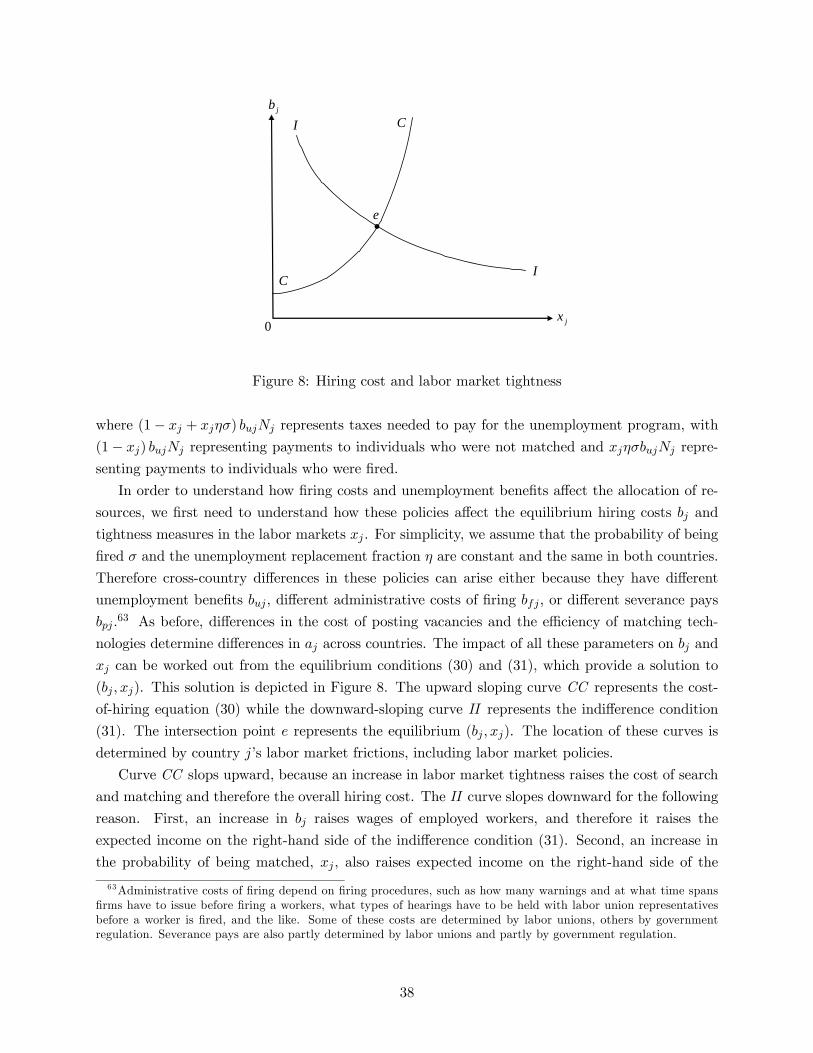
0 jx

I

jbC

e

I

C

•

Figure 8: Hiring cost and labor market tightness

where (1− xj + xjησ) bujNj represents taxes needed to pay for the unemployment program, with

(1− xj) bujNj representing payments to individuals who were not matched and xjησbujNj repre-

senting payments to individuals who were fired.

In order to understand how firing costs and unemployment benefits affect the allocation of re-

sources, we first need to understand how these policies affect the equilibrium hiring costs bj and

tightness measures in the labor markets xj . For simplicity, we assume that the probability of being

fired σ and the unemployment replacement fraction η are constant and the same in both countries.

Therefore cross-country differences in these policies can arise either because they have different

unemployment benefits buj , different administrative costs of firing bfj , or different severance pays

bpj .63 As before, differences in the cost of posting vacancies and the efficiency of matching tech-

nologies determine differences in aj across countries. The impact of all these parameters on bj and

xj can be worked out from the equilibrium conditions (30) and (31), which provide a solution to

(bj , xj). This solution is depicted in Figure 8. The upward sloping curve CC represents the cost-

of-hiring equation (30) while the downward-sloping curve II represents the indifference condition

(31). The intersection point e represents the equilibrium (bj , xj). The location of these curves is

determined by country j’s labor market frictions, including labor market policies.

Curve CC slops upward, because an increase in labor market tightness raises the cost of search

and matching and therefore the overall hiring cost. The II curve slopes downward for the following

reason. First, an increase in bj raises wages of employed workers, and therefore it raises the

expected income on the right-hand side of the indifference condition (31). Second, an increase in

the probability of being matched, xj , also raises expected income on the right-hand side of the

63Administrative costs of firing depend on firing procedures, such as how many warnings and at what time spansfirms have to issue before firing a workers, what types of hearings have to be held with labor union representativesbefore a worker is fired, and the like. Some of these costs are determined by labor unions, others by governmentregulation. Severance pays are also partly determined by labor unions and partly by government regulation.

38

indifference condition (31), because the conditional expected income from being matched (the term

in the square bracket on the right-hand side of (31)) is larger than unemployment benefits.64 As a

result, the II curve slops downward.

Next suppose that A is the rigid country, in the sense that bA > bB, which means that hiring

costs are larger in country A. Unlike the case discussed in previous sections, where differences in

hiring costs emanated from differences in aj across countries, now these differences can arise from

labor market policies concerning firing and unemployment. But whatever generates differences in

bj across countries can be summarized in the ranking bA > bB. Under these circumstances the

results from Section 3 concerning the comparison of outcomes in the differentiated sectors of the

two countries, do not change. In particular, Lemmas 1-4 still hold. That is, if both countries

are incompletely specialized, then the rigid country has a smaller domestic cutoff and a higher

export cutoff, it has a lower real consumption index in the differentiated sector, and it has fewer

firms in that sector. As a result, all the propositions from Section 4 that do not concern welfare

remain valid. For example, Proposition 3 on trade structure and Proposition 5 on productivity

do not change. Moreover, all the propositions concerning welfare also remain valid if there are no

unemployment benefits, or if buj is small.

Propositions concerning welfare can change when buj > 0, because in this case the welfare of

country j depends not only on the real consumption index Qj , but also on aggregate unemployment

benefits that are financed by taxes (see (33)). Different welfare results can arise in this case because

the impact of taxes on welfare can be larger than the impact of real consumption of differentiated

products, and the two of them can influence welfare in opposite directions. As an example consider

a reduction in trade impediments. This raises the real consumption index Qj in both countries,

which is welfare improving. On the other hand, it may attract more workers to the differentiated

sector (Nj may rise). As a result, the unemployment compensation bill may increase, leading to

higher taxes that reduce welfare.65 With high unemployment benefits the latter effect can be larger.

Now consider unemployment in a world of symmetric countries. In this case trade raises unem-

ployment in both of them, because it attracts more workers to the differentiated sectors and does

not changed tightness in the labor markets (see (32)). Moreover, every reduction in trade frictions

raises unemployment.

In contrast, a reduction in hiring costs bj has a more nuanced impact on unemployment. On

the one hand, in a world of symmetric countries a common decline in bj raises Nj in both countries,

because more workers are attracted to the differentiated sectors. On the other hand, tightness in

the labor market xj may rise or decline, depending on what caused bj to fall. To understand why,

we need to discuss the impact of labor market policies on (bj , xj).

An increase in aj or bfj raises directly firms’ labor costs without directly affecting workers’

64We assume that being fired provides higher income than unemployment benefits, i.e., bpj+ηbuj > buj . Thereforewe have σ (bpj + ηbuj) + (1− σ) bj +

12buj > σbuj + (1− σ) bj +

12buj = buj + (1− σ) bj − 1

2buj > buj , where

the last inequality follows from (30).65Note that a decline in τ does not change tightness in the labor markets, so that the cost of the unemployment

program (1− xj + xjησ) bujNj has to increase.

39

payoffs. As a result, it raises the CC curve without affecting the II curve, which implies that bjrises and xj falls. Unlike these parameters, an increase in either bpj or buj raises directly firms’

labor costs and also raises directly workers’ payoffs. As a result, CC shifts upward while II shifts

downward, which implies that xj declines while bj may rise or decline.

We show in the Appendix that

dbjdbpj

< 0 if and only if buj > 1− αajx1+αj .

An example of a case in which buj > 1 − αajx1+αj is the following. Suppose we start from an

equilibrium with no firing costs and no unemployment benefits in country j. Then (30) and (31)

yield xj = a−1/(1+α)j and bj = a

1/(1+α)j / (1− σ). Therefore αajx1+αj > 1 for aj > 1 and α ≥ 1.

Introducing into this country a small severance pay reduces both xj and bj .

One interesting implication of this example is that the introduction of severance pay can raise

welfare. In the example the severance pay reduces hiring costs and thereby raises the real consump-

tion index Qj . Moreover, this policy does not affect taxes, as long as there are no unemployment

benefits. Therefore welfare rises.66 A second interesting implication is that the relationship be-

tween hiring costs and severance pay may be nonmonotonic. If, as in the example, we start with

αajx1+αj > 1, initial increases in severance pay reduce hiring costs. But as severance pay rises,

tightness in the labor market, xj , declines. For high enough levels of severance pay xj is low

enough to reverse the inequality to αajx1+αj < 1. In this new range, increases in severance pay

keep pushing down tightness in the labor market, but now they raise the cost of hiring. Therefore

the relationship between bj and bpj is U shaped.67

We also show in the Appendix that

dbjdbuj

< 0 if and only if buj > 1− αajxαj

∙21− σ (1− η)xj

1− σ− xj

¸.

Note that the term in the square brackets is positive for 0 < xj < 1. Therefore the above inequality

can be satisfied for buj < 1. As an example, consider the case in which σ = 0 (no firing). In this

case (30) and (31) imply

bj = a1

1+α

j (1− buj)α

1+α + 12buj ,

dbjdbuj

=1

2− α

1 + α

µaj

1− buj

¶ 11+α

.

If country j has no unemployment benefits and αa1/(1+α)j / (1 + α) > 1/2, i.e., the right-hand side

of the second equation is negative for buj = 0, then the introduction of unemployment benefits

66Also note that if αajxαj < 1 in the initial equilibrium, the introduction of a small severance pay raises the hiringcost and reduces welfare.67The U shape of this relationship is a more general phenomenon. If buj > 1 − αajx

1+αj for some bpj > 0, then

the same inequality holds for all smaller severance pays. Moreover, since buj < 1 and xj is declining in bpj , it followsthat for large enough values of bpj we have buj < 1− αajx

1+αj . Therefore a necessary and sufficient condition for a

U-shaped relationship between bj and bpj is buj > 1− αajx1+αj when bpj = 0, because xj → 0 as bpj →∞.

40

reduces j’s hiring costs, and the hiring costs are lower the higher the unemployment benefits are.68

Alternatively, suppose that αa1/(1+α)j / (1 + α) < 1/2. Then hiring costs rise with unemployment

benefits when unemployment benefits are low. When unemployment benefits are high, however,

further increases in unemployment benefits reduce hiring costs (dbj/dbuj becomes negative). There-

fore in this case the relationship between hiring costs and unemployment benefits has an inverted

U shape.

Our findings on the determinants of hiring costs and tightness in labor markets can be summa-

rized in

Lemma 6 (i) Increases in aj, bfj, bpj and buj all reduce xj. (ii) Increases in aj and bfj raise bj.

(iii) Increases in bpj and buj can increase or reduce bj. Moreover, the relationship between bj and

bpj can be U shaped, while the relationship between bj and buj can have an inverted U shape.

While the introduction of both severance pay and unemployment benefits can reduce hiring

costs, the introduction of severance pay that reduces hiring costs raises welfare in the absence of

unemployment benefits, while the introduction of unemployment benefits that reduce hiring costs

may reduce welfare. Note that in both cases Qj rises. Yet, while in the case of severance pay an

increase in real consumption of differentiated products guarantees an increase in welfare, in the

case of unemployment benefits it does not, because unemployment benefits have to be financed

with taxes and taxes reduce welfare. Moreover, if the introduction of unemployment benefits raises

hiring costs, then this program is welfare reducing because it leads to higher taxes and lower real

consumption of differentiated products.

It remains to consider the impact of these policies on the trade partner. For this purpose all we

need to know is their impact on hiring costs. If a reform in labor market policies in country j reduces

bj , then country j becomes more competitive in differentiated products, which leads to a contraction

of Q(−j) in the trade partner, as shown in Section 4. Under the circumstances welfare of the trade

partner declines if it has small unemployment benefits, because with small unemployment benefits

the impact on taxes is small. If, however, the trade partner has large unemployment benefits, the

trade partner’s welfare may increase, because the contraction of its differentiated sector reduces

the tax bill for unemployment benefits.

The general conclusion from this analysis is that our results from previous sections concerning

the allocation of resources do not depend on the details of the firing costs and unemployment

benefits, only on the (bj , xj)s, and the welfare results still hold when unemployment benefits are

small. High unemployment benefits can change the welfare results, however, because they impact

taxes needed to finance these benefits. Moreover, the presence of firing costs and unemployment

benefits introduces policy instruments that can change hiring costs and tightness in labor markets

in ways that differ from the impacts of search and matching costs. As a result, they broaden the

set of feasible vectors (bj , xj) and thereby broaden the set of feasible outcomes.

68Under these circumstances unemployment benefits raise unemployment in symmetric countries, because sectoralunemployment rises (xj declines) and more people search for jobs in the differentiated sector (declines in bj raise Nj).

41

8 Concluding Comments

We have studied the interdependence of countries that trade homogeneous and differentiated prod-

ucts with each other, and whose labor markets are characterized by search and matching frictions in

the differentiated-product industry. Variation in labor market frictions and the interactions between

trade impediments and labor market institutions generate rich patterns of unemployment. For ex-

ample, better labor market institutions do not ensure lower unemployment, and unemployment

and welfare can both rise in response to a policy change.

Contrary to the complex patterns regarding unemployment, the model yields sharp predictions

about welfare. In particular, both countries gain from trade, but the gains are unevenly distributed,

with the flexible country gaining proportionately more. The latter implies that a country stands to

gain more from reforming its labor market when trade frictions are low rather than high. Reducing

frictions in the domestic labor market raises the competitiveness of home firms. This improves the

foreign country’s terms of trade, but also crowds out foreign firms from the differentiated-product

sector. As a result welfare rises at home and declines abroad (i.e., the terms-of-trade improvement

in the foreign country is overwhelmed by the competitiveness effect). Nevertheless, across-the-board

improvements in labor market institutions raise welfare in both countries. These results contrast

with the implications of models of pure comparative advantage, in which movements in the terms

of trade dominate the outcomes.69

We also show that labor market institutions confer comparative advantage, and that differences

in these institutions shape trade flows. In particular, the flexible country exports differentiated

products on net and imports homogeneous goods. Moreover, the larger the difference in labor

market frictions the lower is the share of intra-industry trade. These are testable implications

about trade flows and international patterns of specialization.

In addition, we show that trade raises total factor productivity in the differentiated-product

sectors of both countries (productivity is constant in the homogeneous good sector). Importantly,

however, productivity is higher in the flexible country.

We also show how to integrate firing costs and unemployment benefits into this framework. An

interesting implication of these policies is that higher severance pay or higher unemployment benefits

may reduce the cost of hiring, by substantially reducing tightness in the labor market. Under these

circumstances they improve competitiveness. When this type of improvement in competitiveness is

achieved with severance pay, welfare rises. But when this type of improvement in competitiveness

is achieved with unemployment benefits, welfare may decline, because unemployment benefits are

financed with taxes while severance pay is not. Our paper provides an analytical framework for

studying interdependence in the presence of these types of labor market frictions, with interesting

implications for trade and unemployment.

69See, for example, Brügemann (2003) and Alessandria and Delacroix (2008). The former examines the supportfor labor market rigidities in a Ricardian model in which the choice of regime impacts comparative advantage. Thelatter analyzes a two-country model with two goods, in which every country specializes in a different product andgovernments impose firing taxes. The authors find that a coordinated elimination of these taxes yields welfare gainsfor both counties, yet no country on its own has an incentive to do it.

42

Appendix

An alternative specification with homothetic preferences

We consider here an alternative specification of the model, with CRRA-CES preferences instead of quasi-

linear preferences used in the main text, leaving the rest of the setup unchanged. The expected utility is

U = EC1−σ/(1− σ), where E is the expectations operator, σ ∈ [0, 1) is the relative risk aversion coefficientand C is a CES bundle of homogeneous and differentiated goods:

C =hϑ1−ζqζ0 + (1− ϑ)1−ζQζ

i1/ζ, ζ < β, 0 < ϑ < 1.

The ideal price index associated with this consumption bundle is

P =hϑ+ (1− ϑ)P

−ζ1−ζi− 1−ζ

ζ

,

where the price of the homogeneous good p0 is again normalized to one and P is the price of the differentiated

product in terms of the homogeneous good.

The demand for homogeneous and differentiated goods is given by

q0 = ϑPζ/(1−ζ)E =ϑE

ϑ+ (1− ϑ)P−ζ1−ζ

,

Q = (1− ϑ)

µP

P

¶ −11−ζ E

P =(1− ϑ)P

−11−ζE

ϑ+ (1− ϑ)P−ζ1−ζ

,

where E is expenditure in units of the homogeneous good. Using these demand equations, we derive the

indirect utility function

V =1

1− σEµE

P

¶1−σ.

Since P is increasing in P , the indirect utility is falling in P for a given EE1−σ. Also Q is decreasing in P .

Next, the demand level for differentiated varieties is

D ≡ QP1

1−β =(1− ϑ)P

β−ζ(1−β)(1−ζ)E

ϑ+ (1− ϑ)P−ζ1−ζ

,

which increases in P given β > ζ. It proves useful to introduce the aggregate revenue variable

R ≡ PQ = D1−βQβ =(1− ϑ)P

−ζ1−ζE

ϑ+ (1− ϑ)P−ζ1−ζ

,

which, like Q and opposite to D, decreases in P . Note that with homothetic utility, demands and revenues

are linear in income, E, which allows for simple aggregation. Specifically, in the expressions above E can be

interpreted as aggregate income equal to E = (L−N) + wxN .

Most of the remaining derivation of equilibrium conditions remains unchanged, withD replacingQ−(β−ζ)/(1−β)

in the text. Specifically, after this substitution the free entry condition and zero profit conditions are un-

changed, which allows us to solve for equilibrium cutoffs and equilibrium D’s in the same manner as in the

text. Qualitatively all the relationships still hold, except that now instead of Q as the sufficient statistic for

43

welfare and demand level it is more convenient to express all aggregate variables as functions of P . Addi-

tionally, R = PQ replaces Qζ in the expressions forM and N . Finally, the indifference condition for workers

now includes a risk premium for employment seeking in the sector with labor market frictions:

xw1−σ = 1,

so that xw > 1 when x < 1 and there is a chance of being unemployed. The equilibrium wage is still equal

to b = axα, which now leads to

x = b−(1−σ) = a−(1−σ)

1+α(1−σ) ,

w = b = a1

1+α(1−σ) .

Since all workers are indifferent between a certain wage of one in the homogeneous-good sector and the wage

of w with probability x in the differentiated-good sector, we have at the aggregate level EE1−σ = L1−σ, where

expectation is taken both across states for individual workers (employed/unemployed for those searching in

the differentiated sector) and across workers (searching for jobs in the two sectors) and L is the total number

(measure) of individual workers in the economy.

Note that with homothetic preferences and σ < 1, we have dropped the family interpretation. In this

case, the structure of demand and indirect utility does not change if the worker becomes unemployed, and

aggregation is straightforward with EE1−σ = L1−σ and E = L+ (bσ − 1)N .70 As a result, this specificationcan be used to analyze issues such as the ex-post income distribution and winners and losers from policy

reforms.

Without showing the explicit derivation (which follows the same steps as in the text), we provide as an

illustration a few comparative statics results for the symmetric open economies with homothetic preferences.

Specifically, we consider proportional labor market deregulation in both countries. We have D = β/(1−β)b,so that, as before, P decreases and Q and R increase as b falls. This also implies an increase in welfare.

As before, we can express the total wage bill in the differentiated sector as

bH =β

1 + βR =

β

1 + βM(δd + δx)/φ2,

where the δzs are average revenues per entering firm as defined in the text. We still have H = xN . Using

x = b−(1−σ), we have the expression for the number of workers searching for a job in the differentiated sector:

N =β

1 + βb−σR.

Since R is decreasing in b, we have that N decreases in b as before. As a result, there are still two opposing

effects on the unemployment rate: u = b/(b−1)+ N . The change in unemployment rate is again ambiguous:

it still falls if initial labor market institutions are flexible enough and increases otherwise. These results are

qualitatively the same as those derived in the text under quasi-linear preferences.

Additionally, we can discuss now ex post inequality. A fall in b increases x and reduces w, which both

lead to lower ex-post inequality. At the same time it increases N which may increase or reduce inequality

depending on the initial size of the differentiated sector. It follows that comparative statics for inequality is

70Note that if σ ≥ 1, we still need to recur to the family risk-sharing interpretation in order to avoid an infiniterisk premium for employment-seeking in the differentiated product sector with a possibility of being unemployed.Alternatively, the extension of the model with unemployment benefits ensures that the risk premium is finite.

44

ambiguous in the same way as those for unemployment rate.

Complete and Incomplete Specialization Equilibria

We derive here a limit on bA/bB which secures an equilibrium in which both countries are incompletely

specialized. Then we discuss equilibria for which this condition is violated and the rigid country specializes

in homogeneous products. Throughout we assume for concreteness that A is the rigid country, so that

bA/bB ≥ 1. Following the main text, we assume ζ > 0. For brevity, we will analyze only the equilibria withΘxB > ΘdB > Θmin, so that in the flexible country not all producing firms export and there also are firms

that exit. The whole analysis can be carried out in a similar manner when either one of the inequalities fails,

and the results are broadly similar. Finally, for concreteness, we assume that fx ≥ fd. This assumption is

useful because it guarantees that δxB < δdB in the type of equilibria that we consider, which avoids the need

to discuss different cases. Again, the same analysis can be carried out when fx < fd and it yields similar

results.

Equation (20) in the text implies that MA = 0 whenever

δdB

µQA

QB

¶ζ≤ δxB.

When this condition is satisfied with equality we also find, using (16), that

δdB

∙ΘxBΘdB

fdfx

τ−β1−β

¸ζ 1−ββ−ζ

= δxB. (34)

Note that this relationship is a (generally nonlinear) upward-sloping curve in (ΘdB ,ΘxB)-space, lying between

the 45-line and ΘxB = ΘdBτβ/(1−β)fx/fd (i.e., the equilibrium condition when bA = bB).71

We can now prove the following

Lemma 7 Let τ > 1 and bA > bB. Then there exists a unique b(τ), with b0(τ) > 0, such that (34) holds

for bA/bB = b(τ). For bA/bB < b(τ), there is incomplete specialization in equilibrium so that MA > 0. For

bA/bB ≥ b(τ), country A specializes in the homogeneous good so that MA = 0.

Proof: Recall that ΘdB is decreasing and ΘxB is increasing in τ . This implies that δdB/δxB is increasing

in τ . (19) implies that τ−β1−βΘxB/ΘdB is increasing in τ . Next, ΘxB/ΘdB and δdB/δxB are decreasing in

bA/bB. These considerations, together with (34), imply that b(τ) is unique and increasing in τ whenever it

is finite.72 Finally, QA/QB is decreasing in bA/bB . Therefore, from (20), MA > 0 whenever bA/bB < b(τ)

and MA = 0 whenever bA/bB ≥ b(τ).

We consider now equilibria with complete specialization. By Lemma 7 complete specialization in country

A occurs whenever bA/bB ≥ b(τ), so that MA = 0. The equilibrium system in this case consists of five

71 In the special case of a Pareto distribution it is a ray through the origin.72Note that b(τ) > 1 by construction, since ΘxB = ΘdBτ

β/(1−β)fx/fd when bA = bB.

45

equations jointly determining ΘdB ,ΘxB, QA, QB ,MB:

φ1φ2ΘdB = fdbβ

1−βB Q

β−ζ1−βB ,

φ1φ2ΘxB = fxτβ

1−β bβ

1−βB Q

β−ζ1−βA ,

Qβ 1−ζ1−β

A = φ1MBb−β1−βB τ

−β1−β

Z ∞ΘxB

ΘdG(Θ),

Qβ 1−ζ1−β

B = φ1MBb−β1−βB

Z ∞ΘdB

ΘdG(Θ),

fd

Z ∞ΘdB

µΘ

ΘdB− 1¶dG(Θ) + fx

Z ∞ΘxB

µΘ

ΘxB− 1¶dG(Θ) = fe

The first two equations are the cutoff conditions, i.e., counterparts of (16) in the text, but only for country

B now since country A does not produce differentiated goods. The third and fourth equations come from

the definitions of Qjs, as the equations that precede (20) in the text. The final equation is the free entry

condition (17).

The first two equations imply as before

ΘxBΘdB

= τβ

1−βfxfd

µQA

QB

¶β−ζ1−β

. (35)

Taking the ratios of the conditions for QA and QB, we haveµQB

QA

¶β 1−ζ1−β

= τβ

1−βfxfd

ΘdBδdBΘxBδxB

.

The last two results together yield a simple relationshipµQA

QB

¶ζ=

δxBδdB

. (36)

We now are ready to prove

Proposition 10 In equilibrium with specialization (MA = 0), the following comparative statics results hold:

1. ΘdB, ΘxB, and (QA/QB) do not respond to changes in bB. QA and QB fall proportionally in response

to an increase in bB; MB also decreases proportionally with Qζj .

2. ΘdB increases and ΘxB decreases in response to a fall in τ . MB, QB, and QA/QB all increase in

response to a fall in τ . Thus, the rigid country benefits more from a reduction in trade impediments.

Proof: We plug (36) into (35) and take the log-derivative:

ΘxB − ΘdB =β

1− βτ +

β − ζ

ζ(1− β)

³δxB − δdB

´,

where δzB = −hfzΘzBG

0(ΘzB) + δzB

iΘzB for z ∈ d, x. From free entry we have

δdBΘdB + δxBΘxB = 0.

46

Combining these results we have∙δdB + δxB

δxB+ 2δdB + fdΘdBG

0(ΘdB) + fxΘxBG0(ΘxB)

δdBδxB

¸ΘdB = −

β

1− βτ ,

so that ΘdB decreases and ΘxB increases in τ . Also note that neither threshold responds to bB. This result

implies that δdB increases and δxB decreases in τ and they do not respond to bB. This observation together

with (36) imply that QA/QB does not respond to bB and decreases in τ . Log-differentiation of the cutoff

condition for ΘdB results inβ − ζ

1− βQB = −

β

1− βbB + ΘdB.

Therefore, QB and QA fall proportionally as bB increases; QA and QB both decrease in τ and QA does so

proportionally more. Finally, the results for MB follow from the equation for QB:

MB = ζQB − δdB .

Therefore, MB falls in τ ; it also falls in bB at the same rate as QζB .

Proposition 10 emphasizes an important difference between an equilibrium with specialization and an

equilibrium with incomplete specialization (see Proposition 1 in the text). In equilibria with specialization,

the rigid country is the one that gains proportionately more from a reduction in trade impediments. Moreover,

both countries equally gain from improvements in the labor market institutions of the flexible country. The

reason is that now there is no competitiveness effect, which was crowding out the firms in the rigid country

as trade was becoming less costly or as the labor market of the trade partner was becoming more flexible.

Now the only effect is the terms of trade effect, i.e., the reduction in the price level of the differentiated

goods when τ or bB fall. A reduction in trade costs on top of that makes the consumption baskets (i.e., the

number of varieties and their quantities consumed) in the two countries more similar which leads to a partial

convergence in the welfare differential between the countries. Note, however, that both countries still gain

from trade. The reason that the flexible country gains despite the deterioration in its terms of trade is that

the additional profits from the foreign market lead to more entry of domestic firms, which enhances welfare.

Derivation of results on productivity for Section 4.3

We first show that ϕzj = ϕ(Θzj) is monotonically increasing in Θzj. The log-derivative of ϕ(Θzj) is

ϕ(Θzj) = ΘzjG0(Θzj)

"ΘzjR∞

ΘzjΘdG(Θ)

−Θ1/βzjR∞

ΘzjΘ1/βdG(Θ)

#Θzj .

The term in the square brackets is positive since

Θ1/βzjR∞

ΘzjΘ1/β dG(Θ)

1−G(Θzj)<

⎛⎝ ΘzjR∞ΘzjΘ dG(Θ)1−G(Θzj)

⎞⎠1/β

<ΘzjR∞

ΘzjΘ1/β dG(Θ)

1−G(Θzj),

where the first inequality follows from Jensen’s inequality and the second inequality comes from the fact that

β < 1 and Θzj <R∞ΘzjΘ dG(Θ)1−G(Θzj) .

47

Next we provide the general expression for a log-change in aggregate productivity:

[TFP j =

½1 +

κdjϕxj − ϕdj

∙κxjκdj

µΘ

1−ββ

xj − TFP j

¶+

µTFP j −Θ

1−ββ

dj

¶¸¾δdj(ϕxj − ϕdj)

δdjϕdj + δxjϕxjΘdj , (37)

where

κzj ≡ κ(Θzj) =fzΘzjG

0(Θzj)

δzj=

ΘzjG0(Θzj)

1Θzj

R∞ΘzjΘdG(Θ)

.

A series of sufficient conditions can be suggested for the terms in curly brackets to be positive. Since

TFP j > Θ(1−β)/βdj is always true, it is sufficient to require that

TFP j 6 Θ(1−β)/βxj ,

which holds for large enough Θxj , i.e., when the economy is relatively closed. However, this inequality fails

to hold when Θxj approaches Θdj . If this condition fails, it is sufficient to havehTFP j −Θ(1−β)/βdj

i/hTFPj −Θ(1−β)/βxj

i> κxj/κdj ,

which is, in particular, satisfied when κdj > κxj . This latter condition is always satisfied if κ(·) is a non-increasing function and is equivalent to

−ΘG00(Θ)

G0(Θ)≥ 2 + ΘG0(Θ)

1Θ

R∞Θ

ξdG(ξ),

that is G00(·) has to be negative and large enough in absolute value. This condition is satisfied for the Paretodistribution since in this case κ(·) is constant and, thus, κdj ≡ κxj . However, it is not satisfied, for example,

for the exponential distribution.

Finally, the necessary and sufficient condition is¡κxj − κdj

¢TFPj −

³κxjΘ

(1−β)/βxj − κdjΘ

(1−β)/βdj

´6 ϕxj − ϕdj

which is satisfied when¡κxj − κdj

¢ ³TFP j −Θ(1−β)/βdj

´ϕxj − ϕdj

=¡κxj − κdj

¢ "xj +

ϕdj −Θ(1−β)/βdj

ϕxj − ϕdj

#6 1.

This condition also does not hold in general; however, it is certainly satisfied for large enough Θxj .

Now we provide the derivation of equation (26) under the assumption of Pareto-distributed productivity

draws. When Θ is distributed Pareto with the shape parameter k > 1/β, there is a straightforward way of

computing the change in TFP j . Taking the log derivative of (25), we have

[TFPj =

"δdjϕdj δdj + δxjϕxj δxj

δdjϕdj + δxjϕxj− δdj δdj + δxj δxj

δdj + δxj

#+

δdjϕdjϕdj + δxjϕxjϕxjδdjϕdj + δxjϕxj

.

Under the Pareto assumption, the free-entry condition (17) can be written as δdj + δxj = kfe, which implies

48

δdj δdj + δxj δxj = 0. We use this to simplify

[TFP j =δdjϕdj

¡δdj + ϕdj

¢+ δxjϕxj

¡δxj + ϕxj

¢δdjϕdj

.

Next note that δzj = fzk

k−1 (Θmin/Θzj)k so that δzj = −kΘzj and ϕzj =

k−1k−1/βΘ

(1−β)/βzj , implying ϕzj =

(1−β)/βΘzj . Thus, the log-derivative of the free-entry condition can also be written as δdjΘdj+δxjΘxj = 0.

Therefore,

δdj¡δdj + ϕdj

¢= −δxj

¡δxj + ϕxj

¢= −

£k − (1− β)/β

¤δdjΘdj .

Using this, we obtain our result (26) in the text

[TFP j =δdj¡ϕxj − ϕdj

¢£k − (1− β)/β

¤δdjϕdj + δxjϕxj

Θdj .

Finally, we discuss an alternative measure of productivity which takes into account the sectoral composition

of resource allocation:

TFP 0j =L−Nj

L+

Nj

L

Hj

NjTFP j ,

which is a weighted average of 1 (the productivity in the homogeneous sector) and TFP 00j ≡ Hj/Nj ·TFP j

(productivity in the differentiated-product sector). The weights are the respective fractions of the two sectors

in the labor force. Note that \TFP 00j = [TFPj − bj . If TFP 00j > 1, an extensive margin increase in the size

of the differentiated sector improves productivity. Reduction in trade costs and labor market deregulation

additionally shift resources towards the differentiated sector by increasing Nj . These are the additional

effects captured by this alternative measure of aggregate productivity.

Derivation of results for the case of small asymmetries in Section 5.2

For bB = τ = 0 and bA > 0, (19) yield:

ΘdA = −δxA∆(δxB + δdB) bA < 0, ΘxA =

δdA∆(δxB + δdB) bA > 0,

ΘdB =δxB∆

(δxA + δdA) bA > 0, ΘxB = −δdB∆(δxA + δdA) bA < 0.

Using these expressions together with (23) we obtain

β − ζ

1− βQA = −

δdB∆(δxA + δdA) bA < 0,

β − ζ

1− βQB =

δxB∆

(δxA + δdA) bA > 0.

For an initially symmetric equilibrium these expressions become

ΘdA = −δxβ

(1− β) (δd − δx)bA < 0, ΘxA =

δdβ

(1− β) (δd − δx)bA > 0,

ΘdB =δxβ

(1− β) (δd − δx)bA > 0, ΘxB = −

δdβ

(1− β) (δd − δx)bA < 0

49

and

β − ζ

1− βQA = −

δdβ

(1− β) (δd − δx)bA < 0,

β − ζ

1− βQB =

δxβ

(1− β) (δd − δx)bA > 0.

To examine the impact of labor market institutions on unemployment, consider

Qβ 1−ζ1−β

j = φ1

⎡⎢⎣Mjb− β1−β

j

∞ZΘdj

ΘdG (Θ) +M(−j)b− β1−β

(−j) τ−β

1−β

∞ZΘx(−j)

ΘdG (Θ)

⎤⎥⎦ .

Nj = φ1β

1 Mjb− β1−β

j

⎡⎢⎣Q−β−ζ1−β

j

∞ZΘdj

ΘdG (Θ) + τ−β

1−βQ−β−ζ1−β

(−j)

∞ZΘxj

ΘdG (Θ)

⎤⎥⎦ .We differentiate these equations, starting from a symmetric equilibrium with bA = bB, and consider a small

increase in bA. This yields

β1− ζ

1− βQj =σd

∙Mj −

β

1− βbj

¸− μdΘdj + σx

∙M(−j) −

β

1− βb(−j)

¸− μxΘx(−j),

Nj =Mj −β

1− βbj −

β − ζ

1− βσdQj − μdΘdj −

β − ζ

1− βσxQ(−j) − μxΘxj ,

where

σd =

Z ∞Θd

ΘdG (Θ)Z ∞Θd

ΘdG (Θ) + τ−β

1−β

Z ∞Θx

ΘdG (Θ)

and σx = 1− σd < σd

and

μz ≡ σzfzδzG0 (Θz)Θz, z ∈ d, x.

The first two equations can be expressed as

σdMA + σxMB =³−ΨA + βσd

1−β

´bA,

σxMA + σdMB =³ΨB +

βσx1−β

´bA,

where

ΨA ≡β

1− β

1

δd − δx

µβ1− ζ

β − ζδd + μdδx + μxδd

¶> 0,

ΨB ≡β

1− β

1

δd − δx

µβ1− ζ

β − ζδx + μdδx + μxδd

¶> 0.

This system then yields the solution

MA =

µβ

1− β−ΨMA

¶bA, ΨMA ≡

σdΨA + σxΨBσd − σx

,

MB = ΨMB bA, ΨMB ≡σxΨA + σdΨB

σd − σx.

50

Note that

ΨMA −β

1− β>

β

1− β

Ãσd + σx

δxδd

σd − σx

δdδd − δx

β1− ζ

β − ζ− 1!>

β

1− β

µβ1− ζ

β − ζ− 1¶=

βζ

β − ζ> 0.

Therefore, MA unambiguously decreases in bA and MB increases in bA. Also note that as τ → ∞, δx, μxand σx all go to 0 and σd → 1. This implies that ΨMB → 0 as well and ΨMA → β

1−ββ(1−ζ)β−ζ so that MB = 0

and MA = − βζβ−ζ bA, which is exactly the case of the closed economy.

Next we turn to the analysis of Nj, Hj and uj . Using the condition for Nj above and the results for Mj

we have

NA =

∙−ΨMA +

β

1− β

1

δd − δx

nσdδd − σxδx + μdδx − μxδd

o¸bA ≡ −ΨNA bA,

NB =

∙ΨMB −

β

1− β

1

δd − δx

nσdδx − σxδd + μdδx − μxδd

o¸bA ≡ ΨNB bA,

where the first term in the square brackets comes from the changes in Mj and bj and the second term comes

from the change in the thresholds and outputs. Next note that

ΨNA =β

1− β

1

δd − δx

1

σd − σx

∙2σxμdδx + 2σdμxδd + 2σdσx(δd + δx) +

ζ(1− β)

β − ζ(σdδd + σxδx)

¸> 0,

ΨNB =β

1− β

1

δd − δx

1

σd − σx

∙2σxμdδx + 2σdμxδd + 2σdσx(δd + δx) +

ζ(1− β)

β − ζ(σdδx + σxδd)

¸> 0.

When τ →∞, we have ΨNA → βζβ−ζ and ΨNB → 0, and when τ <∞ we have ΨNA > βζ

β−ζ .

Total employment in the differentiated sector changes according to:

HA = NA + xA = −(1 +ΨNA)bA and HB = NB = ΨNB bA

and unemployment responds as

uA = NA −x

1− xxA = −

µΨNA −

1

b− 1

¶bA and uB = NB = ΨNB bA.

Note that if an economy is effectively open (i.e., there is trade in equilibrium) we have

ΨNA −1

b− 1 >βζ

β − ζ− 1

b− 1 .

Therefore, unemployment at home will rise in response to increased flexibility in the home labor market in

an open economy whenever it does so in a closed economy, but not necessarily the opposite.

Solution of the model under the Pareto assumption for Section 5.3

We characterize here the solution of the model under the assumption that productivity draws Θ are dis-

tributed Pareto with the shape parameter k > 2. That is, G(Θ) = 1 − (Θmin/Θ)k defined for Θ ≥ Θmin.We use this characterization in Section 5.3 in order to solve numerically for the equilibrium response of

unemployment to different shocks. In the end of this appendix we provide some analytical results under

Pareto distributed productivity referred to in the text.

51

Pareto-distributed productivity leads to the following useful functional relationship:

δzj ≡fzΘzj

Z ∞Θzj

ΘdG(Θ) = fzk

k − 1

µΘminΘzj

¶k, z ∈ d, x

so that δzj = −kΘdj . As a result, we can rewrite the free entry condition (17) as

fdΘ−kdj + fxΘ

−kxj = (k − 1)feΘ−kmin ⇔ δdj + δxj = kfe.

Manipulating cutoff conditions (16) and the free entry condition above, we can obtain two equations to

solve for Θdj ,Θxj. For concreteness, consider j = A:

fdΘ−kdA+fxΘ

−kxA = (k − 1)feΘ−kmin,

fx

∙τ

β1−β

fxfd

ψ−β

1−β

¸−kΘ−kdA+fd

∙τ

β1−β

fxfd

ψβ

1−β

¸kΘ−kxA = (k − 1)feΘ

−kmin,

where ψ ≡ bA/bB is the relative labor market rigidity of country A. This is a linear system in Θ−kdA ,Θ−kxA

and there are similar conditions for country B, with ψ−1 replacing ψ. The solution to this system is given

by

Θ−kdA =fx∆Θ

"τ

βk1−β

µfxfd

¶k−1ψ

βk1−β − 1

#,

Θ−kxA =fd∆Θ

"1− τ

−βk1−β

µfxfd

¶−(k−1)ψ

βk1−β

#,

where

∆Θ =f2xΘ

kmin

(k − 1)feτ−βk1−β

µfxfd

¶−kψ

βk1−β

"τ

2β1−β

µτ

β1−β

fxfd

¶2(k−1)− 1#> 0.

Using this result we can derive a condition on primitive parameters for Θdj < Θxj to hold in equilibrium:

fdfd + fx

µτ

β1−β

fxfd

¶k+

fxfd + fx

µτ

β1−β

fxfd

¶−k> max

nψ−βk1−β , ψ

βk1−βo, (38)

which is satisfied for large τ and for ψ ≡ bA/bB not very different from one. Next note that as τ → ∞,ΘxA → ∞ and ΘdA →

hfd

(k−1)fe

i1/kΘmin ≡ Θcd. Therefore, the condition for Θcd > Θmin is k < 1 + fd/fe

which is equivalent to the condition in the text. One can also show that ΘdA decreases in τ in the range

τ ∈ (τ∗,∞) where

τ∗ = τ∗(ψ, fx/fd) : (τ∗)βk1−β = (fd/fx)

k−1µψ

βk1−β +

qψ

2βk1−β − 1

¶.

The first cutoff condition in (16) allows to solving for Qj once Θdj is known; Qj is also decreasing in τ

in the range (τ∗,∞). It is straightforward to show that Qj decreases in bA and increases in bB. Using the

Pareto assumption and the equation for Mj (20), we get

Mj = φ2k − 1kΘ−kmin

fdQζjΘ−kd(−j) − fxQ

ζ(−j)Θ

−kx(−j)

f2dΘ−kdAΘ

−kdB − f2xΘ

−kxAΘ

−kxB

. (39)

52

The condition for MA > 0 can then be written asµΘxBΘdB

¶k µQA

QB

¶ζ> 1.

One can show that this inequality imposes a restriction on parameters τ , ψ, fx/fd such that τ > τ∗(ψ, fx/fd),

which implies that Qj is decreasing in τ whenever there is no complete specialization (Mj > 0 for both j).

This is consistent with Lemma 1 in the text.

Finally, using the condition for Nj (21), the the optimal employment levels (6) and conditions (16), we

get

Nj = φ1−ββ

1 φ−12 Mj

£δdj + δxj

¤= φ

1−ββ

1 kfeMj ,

that is, under Pareto assumption, Nj is always proportional with Mj . The remaining equilibrium conditions

are

Hj = Nj/bj and uj = (1− b−1j )Nj/L.

We use the equations above to solve for equilibrium comparative statics numerically. Certain analytical

results can also be obtained under the Pareto assumption for Mj , Nj and uj departing from (39).

Remark for Section 4.3 Under the Pareto assumption we can get a simple prediction about the

response of trade volume to τ , bA and bB . Recall that the total volume of trade (when bA > bB) equals 2XB

where we have

XB = φ−12 MBδxB =δdAδxA

QζB −Qζ

A

δdAδdBδxAδxB

− 1=

fdfx

³ΘxAΘdA

´kQζB −Qζ

A

f2df2x

³ΘxAΘxBΘdAΘdB

´k− 1

=

fdfx

³ΘxAΘdA

´kQζB −Qζ

A

τ2βk1−β

³fxfd

´2(k−1)− 1

.

As bA increases or bB falls, the denominator remains unchanged while ΘxA/ΘdA and QB increase and QA

decreases. As a result the volume of trade unambiguously rises. Finally, one can also show that XB decreases

in τ . Substitute the expression for ΘxA/ΘdA (derived from (16)) in the expression for XB to get

XB = QζA

τβk1−β

³fxfd

´k−1 ³QB

QA

´ζ+k β−ζ1−β − 1

τ2βk1−β

³fxfd

´2(k−1)− 1

.

Now note that XB decreases in τ since QA and QB/QA decrease in τ and QB > QA.

Proof of Proposition 7 In the text we show that NA + NB increases as τ falls. We show now that

when bA > bB, NA/NB decreases as τ falls, which implies that NB necessarily increases. Under the Pareto

assumption δdj + δxj = kfe. Therefore, (20) and (21) imply

NA

NB=

MA

MB=

δdBQζA − δxBQ

ζB

δdAQζB − δxAQ

ζA

=

1− δxBkfe

∙1 +

³QB

QA

´ζ¸δdAkfe

∙1 +

³QB

QA

´ζ¸− 1

< 1,

where the last inequality comes from Lemma 4 under the assumption that bA > bB . From Proposition 1,

QB/QA increases as τ falls. Taking this and the fact that NA < NB into account, it is sufficient to show

53

that dδxB −dδdA = δxB δxB − δdAδdA > 0 in response to a fall in τ , to establish that NA/NB declines in this

case. Under the Pareto-distributed productivity,

δxB δxB − δdAδdA = k³δdAΘdA − δxBΘxB

´= k

(δdBδxB − δdAδxA)(δdA − δxA)

∆

¡− τ

¢> 0,

where the second equality comes from (19) and the inequality is obtained by Lemma 3 and the fact that

under the Pareto assumption δdA + δxA = δdB + δxB = kfe. This proves that NB increases as τ falls when

bA > bB . Since changes in τ do not affect labor market tightness, xB, the only effect on the unemployment

rate uB is through NB , and hence the unemployment rate in the flexible country increases in response to

trade liberalization.

Proof of results for Section 6.2

Consider the equilibrium system in the case when there are trade frictions in the homogeneous-good sector

and country B has a more flexible labor market (bA > bB). As described in the text, the free entry condition

is still given by (17) and is the same for both countries. The production cutoff is given by the following zero

profit condition:

πdj(Θdj) = p0j£φ1φ2b

− β1−β

j Q−β−ζ1−β

j Θdj − fd¤= 0

and hence defines a symmetric condition for both countries independently of p0j . The only asymmetry is in

the export cutoff condition:

πxj(Θxj) = p0j£φ1φ2τ

− β1−β b

− β1−β

j

¡p0(−j)/p0j

¢ 11−β Q

−β−ζ1−β

(−j) Θxj − fx¤= 0.

We want to find the value of p0B/p0A = τ0, for a given ratio bA/bB > 1, such that ΘxA = ΘxB. The free

entry condition then implies ΘdA = ΘdB and the production cutoff condition impliesµbAbB

¶ β1−β

=

µQB

QA

¶β−ζ1−β

.

Using this, the export cutoff conditions result in

τ0 =

µbAbB

¶β.

Now taking the full derivative of the equilibrium system, we obtain the following comparative statics:

ΘdA = −δxB∆(δdB + δxB)

¡bA − bB − τ0/β

¢,

ΘdB = −δxA∆(δdA + δxA)

¡bB − bA + τ0/β

¢.

This implies that ΘdB/ΘdA is decreasing in τ0(bB/bA)β , and from previous discussions we know that ΘdA =

ΘdB when τ0¡bB/bA

¢β= 1. This proves that ΘdA < ΘdB if and only if τ0 <

¡bA/bB

¢β. This also implies

δdA > δdB . >From the free entry condition we know that the same restriction is necessary and sufficient

for ΘxA > ΘxB, which also implies δxA < δxB. From the domestic production cutoffs conditions, we then

know that this restriction implies QB/QA >¡bA/bB

¢β/(β−ζ)> 1, and hence is sufficient but not necessary

for QB > QA.

54

Finally, solving for Mjs as in Section 3, we have

MA −MB =(1− β)φ2

β∆

h(δdB + δxA/τ0)Q

ζA − (δdA + τ0δxB)Q

ζB

i.

Therefore, the discussion above implies that τ0 <¡bA/bB

¢βis also sufficient, but not necessary, for MB >

MA. Recall that the condition for net trade in the differentiated good, MAδxA < MBτ0δxB, is therefore also

satisfied, which implies that it is valid to do the comparative statics on the equilibrium system above when

τ0 ≤¡bA/bB

¢β.

Note thatMAδxA < MBτ0δxB is satisfied with slack when τ0 =¡bA/bB

¢β. Therefore, for a given bA/bB,

τ and other parameters of the model, there exists a τ0 >¡bA/bB

¢βsuch that MAδxA < MBτ0δxB holds if

and only if τ0 < τ0.73

Whenever τ0 < τ0, we have equilibrium with intersectoral trade. In this case, the equilibrium system is

as described above. Moreover, the comparative statics results with respect to bA, bB and τ are still given by

(19) and (23). Since the ranking of δzjs is preserved when τ0 <¡bA/bB

¢β, all the results of Section 4 still

apply in this case. When, however, τ0 >¡bA/bB

¢β, we have δxA > δxB and δdA < δdB, which implies that

country A gains more from trade, while other comparative statics results are unchanged.

Finally, note from the comparative statics above that when τ0 < τ0, ΘdA is increasing and ΘdB is

decreasing in τ0. Domestic production cutoff conditions then imply that QA increases and QB decreases

in τ0.

Proof of results for Section 7

We reproduce here equations (30):74

b =axα + σ(bf + bp)

1− σ+1

2bu,

and substitute it into (31) to obtain:

x [axα + σbf + 2σbp − σ(1− η)bu] = 1− bu.

Note that this last expression implicitly determines x as a function of the labor market characteristics.

Taking the full differential, we have£1− bu + αax1+α

¤x =− ax1+αa− σxdbf − 2σxdbp,− [1− σ(1− η)x]dbu,

where as before a hat denotes log-derivative so that x = dx/x. This immediately implies that x decreases in

all labor market parameters, a, bf , bp and bu.75

Next, the full differential for b is given by

db =αax1+α

1− σx+

1

1− σ

£axαa+ σ(dbf + dbp)

¤+1

2dbu.

73We do not prove here that τ0 is finite. However, it is immediate to see that as bA/bB → 1, τ0 → 1, that is thereis no intersectoral trade around the symmetric equilibrium with arbitrarily small trade frictions in the homogenousgood.74We drop subscript j in this appendix as it causes no confusion.75One can additionally show that x decreases in σ and η.

55

Note that the direct effect of all labor market parameters on b is positive. However, they all have negative

indirect effects on b through labor market tightness, x. Formally, combining the expressions for db and x,

we have:

db =+(1− bu)ax

α

(1− σ)£1− bu + αax1+α

¤ a+

σ

1− σ

1− bu1− bu + αax1+α

dbf

+σ

1− σ

1− bu − αax1+α

1− bu + αax1+αdbp

+

"1

2−

αaxα£1− σ(1− η)x

¤(1− σ)

£1− bu + αax1+α

¤# dbu.Note that b always increases in a and bf . Yet, it may increase or decrease in bp and bu. It decreases in

bp whenever 1 − bu < αax1+α, as stated in the text. The condition for b to decrease in bu is slightly more

complex. One way to write it is as given in the text:

1− bu < αaxα∙21− σ(1− η)x

1− σ− x

¸.

When σ = 0, it collapses to

1− bu < αaxα(2− x).

Moreover, in this case the expression for x becomes 1 − bu = ax1+α, so that we can rewrite the condition

above as

x < α(2− x) or x < 2α/(1 + α),

which is equivalent to the expression in the text.

56

References

[1] Agell, Jonas and Per Lundborg (1995), "Fair Wages in the Open Economy," Economica 62,

pp. 335—351.

[2] Alessandria, George and Alain Delacroix (2008), “Trade and the (Dis)Incentive to Reform La-

bor Markets: The Case of Reform in the European Union,” Journal of International Economics

75, pp. 151-166.

[3] Amiti, Mary and Christopher Pissarides (2005), "Trade and Industrial Location with Hetero-

geneous Labour," Journal of International Economics 67, pp. 392-412.

[4] Bernard, Andrew B. and J. Bradford Jensen (1995), “Exporters, Jobs, and Wages in US

Manufacturing: 1976-87,” Brookings Papers on Economic Activity: Microeconomics, pp. 67-

112.

[5] Blanchard, Olivier and Jordi Gali (2008), “Labor Markets and Monetary Policy: A New-

Keynesian Model with Unemployment," NBER Working Paper No. 13897.

[6] Blanchard, Olivier and Justin Wolfers (2000), "The Role of Shocks and Institutions in the Rise

of European Unemployment: The Aggregate Evidence," Economic Journal 110, pp. C1-C33.

[7] Botero, Juan C., Simeon Djankov, Rafael La Porta, Florencio Lopez-de-Silanes and Andrei

Shleifer (2004), "The Regulation of Labor," Quarterly Journal of Economics 119, pp. 1339-

1382.

[8] Brecher, Richard (1974), "MinimumWage Rates and the Pure Theory of International Trade,"

Quarterly Journal of Economics 88, pp. 98-116.

[9] Brecher, Richard (1992), "An Efficiency-Wage Model with Explicit Monitoring: Unemploy-

ment and Welfare in an Open Economy," Journal of International Economics 32, pp. 179-191.

[10] Brügemann, Björn (2003), “Trade Integration and the Political Support for Labor Market

Rigidity,” mimeo, Yale University.

[11] Chor, Davin (2006), "Unpacking Sources of Comparative Advantage: A Quantitative Ap-

proach," mimeo, Harvard University.

[12] Copland, Brian (1989), "Efficiency Wages in a Ricardian Model of International Trade," Jour-

nal of International Economics 27, pp. 221-244.

[13] Costinot, Arnaud (2006), "On the Origins of Comparative Advantage," mimeo, UCSD.

[14] Cuñat, Alejandro and Marc Melitz (2007), "Volatility, Labor Market Flexibility, and the Pat-

tern of Comparative Advantage," NBER Working Paper No. 13062.

57

[15] Davidson, Carl, Lawrence Martin and Steven Matusz (1988), "The Structure of Simple General

Equilibrium Models with Frictional Unemployment," Journal of Political Economy 96, pp.

1267-1293.

[16] Davidson, Carl, Lawrence Martin and Steven Matusz (1999), "Trade and Search Generated

Unemployment," Journal of International Economics 48, pp. 271-299.

[17] Davidson, Carl and Steven Matusz (2006a), "Long-run Lunacy, Short-run Sanity: a Simple

Model of Trade with Labor Market Turnover," Review of International Economics 14, pp.

261-276.

[18] Davidson, Carl and Steven Matusz (2006b), "Trade Liberalization and Compensation," Inter-

national Economic Review 47, pp. 723-747.

[19] Davis, Donald (1998), "Does European Unemployment Prop Up American Wages? National

Labor Markets and Global Trade," American Economic Review 88, pp. 478-494.

[20] Davis, Donald and James Harrigan (2007), "Good Jobs, Bad Jobs, and Trade Liberalization,"

mimeo, Columbia University.

[21] Demidova, Svetlana (2006), "Productivity Improvements and Falling Trade Costs: Boon or

Bane?" International Economic Review (forthcoming).

[22] Egger, Harmut and Udo Kreickemeier (2006), "Firm Heterogeneity and the Labour Market

Effects of Trade Liberalization," GEP Research Paper 2006/26.

[23] Fariñas, José C. and Ana Martín-Marcos (2007), "Exporting and Economic Performance:

Firm-Level Evidence of Spanish Manufacturing," The World Economy 30, 618-646.

[24] Felbermayr, Gabriel, Julien Prat and Hans-Jörg Schmerer (2008), "Globalization and Labor

Market Outcomes: Wage Bargaining, Search Frictions, and Firm Heterogeneity," IZA Discus-

sion Papers 3363.

[25] Harris J. and M. Todaro (1970), “Migration, Unemployment and Development: A Two-Sector

Analysis," American Economic Review 60, 126-142.

[26] Helpman, Elhanan and Paul R. Krugman (1985), Market Structure and Foreign Trade (Cam-

bridge, MA: MIT Press).

[27] Helpman, Elhanan, Oleg Itskhoki and Stephen Redding (2008a), "Wages, Unemployment and

Inequality with Heterogeneous Firms and Workers," mimeo.

[28] Helpman, Elhanan, Oleg Itskhoki and Stephen Redding (2008b), "Inequality and Unemploy-

ment in a Global Economy," in preparation.

[29] Hoon, Hian Teck (2001), "Adjustment of Wages and Equilibrium Unemployment in a Ricardian

Global Economy," Journal of International Economics 54, pp. 193-209.

58

[30] Hosios, Arthur J. (1990), "Factor Market Search and the Structure of Simple General Equi-

librium Models," Journal of Political Economy 98, pp. 325-355.

[31] Jones, Ronald W. (1965), "The Structure of Simple General Equilibrium Models," Journal of

Political Economy 73, pp. 557-572.

[32] Kreickemeier, Udo and Douglas Nelson (2006), "Fair Wages, Unemployment and Technological

Change in a Global Economy," Journal of International Economics 70, pp. 451—469.

[33] Levchenko, Andrei A. (2007), "Institutional Quality and International Trade," forthcoming in

the Review of Economic Studies 74, pp. 791-819.

[34] Matusz, Steven J. (1986), "Implicit Contracts, Unemployment and International Trade," Eco-

nomic Journal 96, pp. 71-84.

[35] Melitz, Marc J. (2003), "The Impact of Trade on Intra-Industry Reallocations and Aggregate

Industry Productivity," Econometrica 71, pp. 1695-1725.

[36] Mitra, Devashish and Priya Ranjan (2007), "Offshoring and Unemployment," mimeo, Syracuse

University.

[37] Moore, Mark P. and Priya Ranjan (2005), "Globalisation vs Skill-Biased Technological Change:

Implications for Unemployment and Wage Inequality," Economic Journal 115, pp. 391-422.

[38] Nickell, Steven (1997), "Unemployment and Labor Market Rigidities: Europe Versus North-

America," Journal of Economic Perspectives 11, pp. 55-74.

[39] Nickell, Steven, Luca Nunziata, Wolfgang Ochel and Glenda Quintini (2002), "The Beveridge

Curve, Unemployment and Wages in the OECD from the 1960s to the 1990s," Center for

Economic Performance, the LSE.

[40] Nunn, Nathan (2007), "Relationship-Specificity, Incomplete Contracts, and the Pattern of

Trade," Quarterly Journal of Economics CXXII, pp. 569-600.

[41] Pissarides, Christopher A. (2000), Equilibrium Unemployment Theory (Cambridge, MA: The

MIT Press, second edition).

[42] Stole, Lars A. and Jeffrey Zwiebel (1996a), “Organizational Design and Technology Choice

under Intrafirm Bargaining,” American Economic Review 86, pp. 195-222.

[43] Stole, Lars A. and Jeffrey Zwiebel (1996b), “Intra-Firm Bargaining under Non-Binding Con-

tracts,” Review of Economic Studies 63, pp. 375-410.

59