Embed Size (px)
Citation preview

Prof. dr. Davor Eterović, editor
Authors:
D. Eterović, D. Kovačić, V. Marković, A. Punda
Laboratory exercises:
Medical physics and biophysics/2012-13
Department of Medical Physics and Biophysics
University of Split – School of Medicine

Original title:
Upute za vježbe – Medicinska fizika i biofizika
Katedra za medicinsku fiziku i biofiziku, Sveučilište u Splitu-Medicinski fakultet
Translated by:
1. M. Raguž (exercises 1,2,5,8 and 9)
2. D. Eterović (exercises 3,4 and 10)
3. D. Kovačić (exercises 6 and 7)
Laboratory exercises: Medical physics and biophysics 2012/13
Students are obliged to study the following instructions for exercises and to consult the texts of the
corresponding lectures.
Exercise
Place
E1: Radioactivity and radiation protection Dept. of Nucl. Med.
E2: Absorbed radiation dose Dept. of Nucl. Med.
E3: Measurements in nuclear medicine Dept. of Nucl. Med.
E4: Radiogram contrasts BSB: Laboratory
E5: Echogram resolution Dept. of Oncology
E6: Neural signal BSB: Laboratory
E7: Audiometry BSB: Laboratory
E8: Optical bench BSB: Laboratory
E9: Viscosity BSB: Laboratory
E10: Hemodynamic BSB: Laboratory
1. Department of Nuclear Medicine; University Hospital Split; location Firule, Spinčićeva 1
2. Department of Oncology; University Hospital Split; location Firule, Spinčićeva 1
3. BSB: Laboratory; Basic Science Building, Medical Faculty Split; location Križine, Šoltanska 2
Exercise 1: Radioactivity and protection of radiation
Radioactivity:
Process in which energetically unstable atomic nuclei spontaneously changes (decay) because of the
transition to a lower energy state.
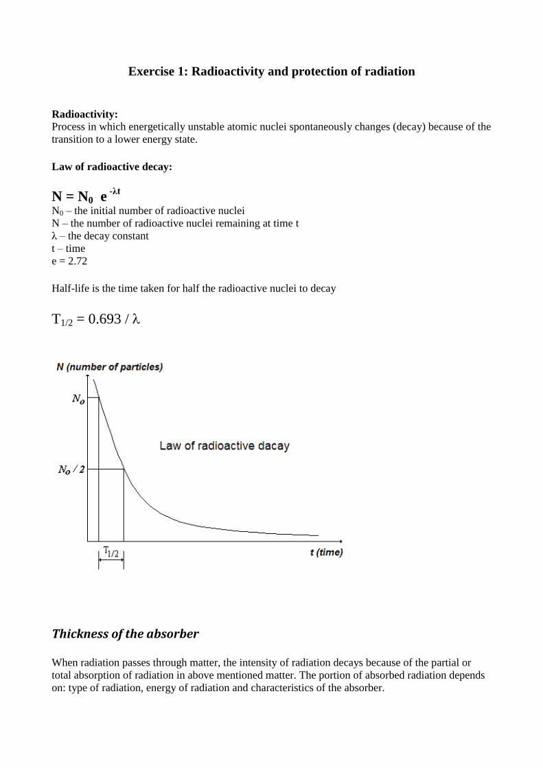
Law of radioactive decay:
N = N0 e -λt
N0 – the initial number of radioactive nuclei
N – the number of radioactive nuclei remaining at time t
λ – the decay constant
t – time
e = 2.72
Half-life is the time taken for half the radioactive nuclei to decay
T1/2 = 0.693 /
Thickness of the absorber
When radiation passes through matter, the intensity of radiation decays because of the partial or
total absorption of radiation in above mentioned matter. The portion of absorbed radiation depends
on: type of radiation, energy of radiation and characteristics of the absorber.
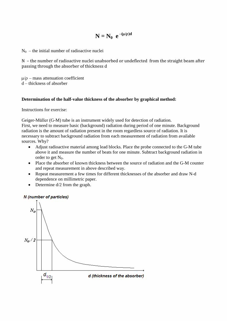
N = N0 e –(/)d
N0 – the initial number of radioactive nuclei
N – the number of radioactive nuclei unabsorbed or undeflected from the straight beam after passing through the absorber of thickness d
/ – mass attenuation coefficient
d – thickness of absorber
Determination of the half-value thickness of the absorber by graphical method:
Instructions for exercise:
Geiger-Müller (G-M) tube is an instrument widely used for detection of radiation.
First, we need to measure basic (background) radiation during period of one minute. Background
radiation is the amount of radiation present in the room regardless source of radiation. It is
necessary to subtract background radiation from each measurement of radiation from available
sources. Why?
Adjust radioactive material among lead blocks. Place the probe connected to the G-M tube
above it and measure the number of beats for one minute. Subtract background radiation in
order to get N0.
Place the absorber of known thickness between the source of radiation and the G-M counter
and repeat measurement in above described way.
Repeat measurement a few times for different thicknesses of the absorber and draw N-d
dependence on millimetric paper.
Determine d/2 from the graph.
Protection from radiation
1. Principles of protection:
- Source of radiation (type of radiation, dose)
- Time
- Distance (I~1/R2)
- Shields
2. Radiation dosimetry:
- Personal dosimeters (ionization chamber, radiographic film, thermoluminiscent
dosimeter)
Demonstrate influence of each particular principle of protection at decrease of exposure using
personal dosimeter (ionization chamber).
Measurement of the relative gamma constant (Γ)
Read lesson Dosimetry in the chapter Ionizing radiation, contained in the material entitled
Biophysics lectures 2011-2 /Diagnostics (PDF file at the Web site).
You have an access to two different sources of ionization radiation: 131
I and 99m
Tc.
1. Measure their activities using G-M tube
2. Measure rates of exposures at the same ‘spot’ in the space (at the distance R from each
particular source of radiation) using personal dosimeter.
3. Calculate gamma constant of 131
I based on performed measurements and using the next
equation:
Rate of exposure =ΓA/R2
Gamma constant of radioactive isotope 99m
Tc is equal 0.14 Cm2/kgBqs x 10
14.
Exercise 2: Absorbed dose
The subject of exercise and what you should do
This exercise shows the method of planning the therapy of hyperfunctioning thyroid gland with
exposure to ionizing radiation from the beta emitter I-131, given orally in form of potassium or
sodium iodide. Upon entering the circulation, the radioactive iodine cations (along with stable
counterparts) are ether excreted by kidneys or trapped by thyroid, initiating the process of thyroid
hormone production. This process takes several days during which the beta radiation from I-131 is
absorbed in the gland. The goal is to partly destroy the thyroid tissue, ideally so that the remaining
parts ensure normal production of thyroid hormones. However, the treatment is also considered
relatively successful in case of over-destruction and consequent low hormone production (the
patient then regularly takes the synthetic hormone supplements).
The student is not expected to perform the measurements on a patient, but to study this material and
be able to follow the instructor.
Basics
The chapter Dosimetry/Biophysics lectures- diagnostics (accessible at the Faculty web pages) can
serve as an introduction to this exercise. This section scrutinizes the most important aspects from
that material:
In traversing matter the ionizing radiation exerts effects that may be only temporary (in case of non-
living material) or chronic and serious ones (living tissue). The radiation effects depend on:
(i) intensity of radiation at the point of interest
(ii) interaction probabilities of radiation with matter, and
(iii) duration of exposure
These effects are quantified by:
Absorbed dose, which is the energy the radiation deposited to unit absorber mass. The unit is Grey
(Gy). One Grey is 1 Joule/kilogram (J/kg). Absorbed dose indicate cumulative effects of ionizing
radiation on the unit mass of the exposed medium during non-specified time spent in radiation field.
Dividing with time, one gets the time independent quantity; the absorbed dose rate, measured in
Gy/s.
One should realize that the small amounts of this energy can do a lot of harm to living tissue. This is
explained by the mechanism of energy absorption. Unlike non-ionizing radiations, which give-off
energy by increasing the rate of molecular rotations and vibrations, high energy photons or particles
ionize atoms, creating positive ions and free electrons. Subsequently, the ejected electrons are
slowed down and recaptured by positive ions. When the radiation exposure ceases, the non-living
material is usually left unchanged. However, the living tissue is sensitive to periods when free ions
exist. Molecules of a living tissue continuously interact in a precise manners and ionization may
interfere with these delicate processes. Radiation harms cells by ionizing biologically important
molecules like DNA, which is the direct effect, or by chemically altering intracellular water, which
is indirect effect.
Biological damage inflicted by ionizing radiation does not depend only on absorbed dose; the type
of radiation matters also. Namely, large number of ionizations within a single cell, or single
macromolecule, is more harmful than the same number of ionizations (and thus absorbed energy)
distributed over more cells (molecules). Neutrons and alpha particles ionize very densely, producing
more commonly multiple, irreparable damages, than gamma or beta radiation. To account for this,
one defines the equivalent dose:
Equivalent dose = Q.Absorbed dose
where Q is quality factor. In case of alpha particles Q is 20, for neutrons range 5 to 20 applies
(depending on energy), while beta particles and gamma photons have Q=1. The unit of equivalent
dose is Sievert (Sv). The old unit is rem (1 rem=0.01 Sv).
Besides, the sensitivity to radiation (radiosensitivity) depends on type of tissue (rate of proliferation
is essential!). So, we also introduce the quantity called effective equivalent dose. To each part of a
body one assigns the specific weight factor, which accounts for differential radiosensitivity. The
effective equivalent dose equals the product of the weight factor and equivalent dose in the part of
body considered. The unity is also Sievert. To summarize, the effects of radiation on a living tissue
depend on:
(i) part of body exposed (cells that divide intensively are most sensitive)
(ii) absorbed dose
(iii) type of ionizing radiation (heavier particles ionize more densely)
(iv) absorbed dose rate (longer time enables recuperation)
The examples of radiation effects are: skin burns, nausea, hair loss, sterility, cataract, bone marrow
damage, changes in genes and induction of carcinoma. Excessive doses may cause death in a couple
of days. However, we may also purposely expose the parts of a body to ionizing radiation in order
to destroy malignant or hyper-functioning tissue.
Therapy with emitters of ionizing radiation
In cases of some malignant and non-malignant diseases the emitters of ionizing radiation are
entered in body of a patient with intention to destroy or permanently damage the specific tissue
cells. This can be achieved by placing the solid source near the target tissue (brachytherapy), or by
entering the emitter in blood, bound to specific carrier, which provides for accumulation in the
target organ. In the later case, the compounds containing beta emitters are either given orally or
injected intravenously. Occasionally, the carrier is the radioisotope atom (ion) itself, as is the case
of 131
I cation when thyroid is the target organ. Such procedures must be carefully planned in order
that the damage is restricted to target tissue and to avoid both under-destruction and over-
destruction (especially in case of non-malignant diseases). To accomplish this one must take into
account the individual patient characteristics.
Clinical problem
Hyperthyroidism is a condition characterized by excessive thyroid hormone production. The
surplus of thyroid hormones in body cells accelerates the metabolism in virtually all tissues. The
symptoms include increased heart rate, tremor, sweating, insomnia, chronic fatigue and loss of
weight, despite increased food intake. There are several underlining diseases: diffuse toxic goitre
(Graves-Basedow disease), toxic adenoma (thyroid nodule which lost pituitary control and
functions autonomously), toxic multinodular goitre or, rarely, pituitary adenoma. All these
diseases cause thyroid overfunctioning (i.e. hyperthyroidism) and consequent increased serum
concentrations of thyroid hormones (thyrotoxicosis). However, thyrotoxicosis may also be related
to several other conditions/diseases. For example, some inflammatory thyroid diseases damage the
thyroid tissue, causing leakage of internal hormone reserves and transient thyrotoxicosis. Next, the
patient with hypothyroidism (the state of insufficient production of thyroid hormones) may be
overtreated with synthetic thyroid hormones, or, rarely, there may be the case of hormonally active
tumours.
First one establishes the diagnosis of hyperthyroidism, which is related to disorders of thyroid tissue
(i.e. excludes other causes of thyrotoxicosis and abnormal pituitary functioning). The treatment than
usually begins (in Europe) with antithyroid drugs. This, however, is successful only in fraction of
patients. In patients who do not respond adequately to antithyroid drugs there are two kinds of
definitive treatments: surgery or radioiodine. In USA, Japan, and in some European centres
relatively large, so called ablative radioactive doses are planned, with goal to quickly achieve the
cessation (remission) of hyperthyroid state. The price paid is thyroid overdestruction and the patient
usually becomes hypothyroid. In majority of European centres one tries the individual dosimetric
approach, aiming not only for remission of hyperthyroidism, but for normal thyroid function, e.g.
euthyroidism.
Therapy planning
In Croatia about 90% of hyperthyroidism is due to diffuse toxic goitre, and we will focus on this
disease. The thyroid absorbed dose necessary to achieve the euthyroid state varies from patient to
patient. The reasons behind this individual radiosensitivity of thyroid tissue are not yet well
understood and the success of therapy cannot be accurately predicted. Sometimes the absorbed dose
is too small and the patient remains hyperthyroid (requiring retreatment), or it is too big and the
patient becomes hypothyroid. Current data indicate that 120 Gy is the thyroid absorbed dose (due to
beta/gamma radiation from I-131) that most frequently results in euthyroidism (in about 2/3 cases).
Whether better results can be achieved by recognizing the signs of individual patient
radiosensitivity is currently being investigated in several centres, including the Department of
Nuclear Medicine, University Hospital Split. Since I-131 is the beta/gamma emitter the absorbed
dose of 120 Gy corresponds to equivalent dose of 120 Sv.
For each patient one should determine the activity (radioactivity) of I-131 that, that upon oral
application, ends-up in thyroid in adequate quantity to produce the desired (planned) absorbed dose.
Given the planned absorbed dose (usually around 120 Gy), the required activity increases with
thyroid mass (recall that absorbed dose relates to unit absorber mass) and decreases with fraction of
given activity that ends-up in thyroid (the rest is eliminated by kidneys). This fraction is measured
at 24 hours after oral application of radioiodine and is called 24 h uptake. Also, the longer
radioiodine spends in thyroid (the greater effective half-life of radioiodine attached to thyroglobulin
molecule), the greater absorbed dose and the less radioiodine activity is required.
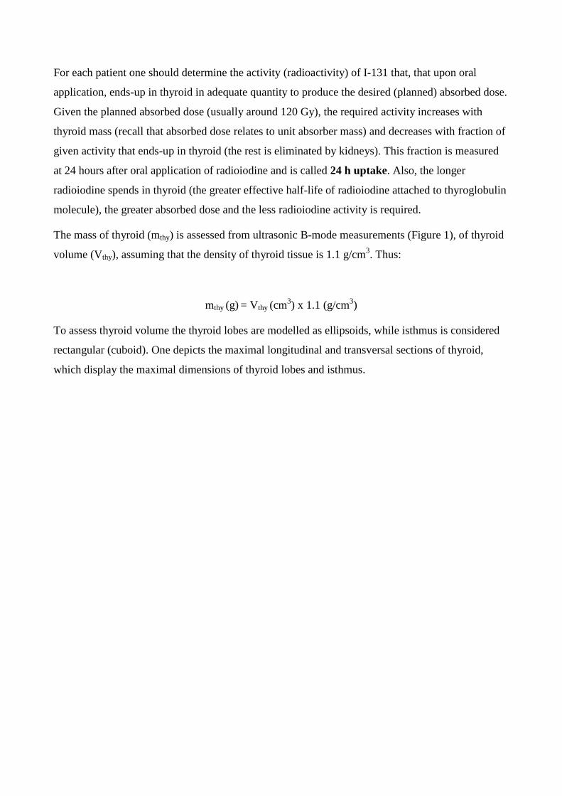
The mass of thyroid (mthy) is assessed from ultrasonic B-mode measurements (Figure 1), of thyroid
volume (Vthy), assuming that the density of thyroid tissue is 1.1 g/cm3. Thus:
mthy (g) = Vthy (cm3) x 1.1 (g/cm
3)
To assess thyroid volume the thyroid lobes are modelled as ellipsoids, while isthmus is considered
rectangular (cuboid). One depicts the maximal longitudinal and transversal sections of thyroid,
which display the maximal dimensions of thyroid lobes and isthmus.
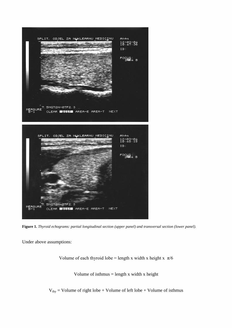
Figure 1. Thyroid echograms: partial longitudinal section (upper panel) and transversal section (lower panel).
Under above assumptions:
Volume of each thyroid lobe = length x width x height x π/6
Volume of isthmus = length x width x height
Vthy = Volume of right lobe + Volume of left lobe + Volume of isthmus
The measurement of 24 h uptake is performed separately using the open collimator counter. Using
the same geometry, the count rate of radiation emanating from the patient neck at 24 hour after
application of radioiodine are divided by the count rate due to bottle with radioactivity to be given
to the patient the day before (see Exercise 4). This ratio, corrected for I-131 decay and slightly
different efficacies of two measurements, is 24 h uptake (around 20% in normal thyroid, from 60-
80% in hyperthyroidism). These measurements can be repeated at several consecutive days. From
these data the effective half-life of radioiodine in thyroid is calculated.
So called Marinelli’s formula relates the activity of I-131 that is required to induce the planned
absorbed dose, taking into account 24 h uptake and effective half-life of radioiodine in thyroid
(Appendix):
(%)uptakeh24x)days(lifehalfeffective
7.24x)g(mx)Gy(doseabsorbedplanned)MBq(activity131I
thy
The simpler method uses the other formula:
I-131 activity (µCi) = uptakeh24
Ci300100x)g(mthy
To apply the above formula a physician needs to choose the planned absorbed dose (for example
120 Gy). This then determines the factor 100-300 µCi in the nominator. Note that the method is
only semiquantitaitve one, sine the formula does not contain the effective half-life of radioiodine in
thyroid. In this way one neglects the individual variations in this quantity, assuming the empirical
average value. The price paid is loss of precision; the gain is in simplicity, by avoiding multiple
measurements of thyroid uptake in several days.
Appendix: Derivation of Marinelli’s formula
The great majority of I-131 radiation energy absorbed in thyroid comes from beta electrons. So, we
will first neglect the fraction of absorbed dose coming from accompanying gamma radiation.
Assuming that all beta electrons are absorbed within thyroid tissue, the energy deposited equals the
total number of I-131 disintegrations in thyroid multiplied by average beta electron energy (190
keV):
Energy absorbed by whole thyroid = Total number of I-131 disintegrations x 190 keV
We next assume that, upon oral application, all radioiodine is instantaneously trapped in the gland.
Then the total number of I-131 disintegrations in thyroid equals the product of the initial I-131
activity present in thyroid (the activity orally given multiplied by thyroid uptake), multiplied by
average time the radioiodine spends in the gland (Taverage):
Energy absorbed by whole thyroid = I-131 activity x 24 h uptake x Taverage x 190 keV
Taverage is obtained as the weighted average of all times (from zero to infinity); the weight factor is
proportional totefe
, where λef is the constant of effective elimination of radiotracer from thyroid
(both due to physical decay and biological elimination; i.e. secretion of hormones containing
radioactive iodine). The constant of proportionality is obtained by normalizing the area under the
curve tefe
(t>0) to unity. By using the methods of integral calculus one obtains:
Taverage = ef
1
This can be written as (see Dosimetry/Biophysics lectures- diagnostics):
Taverage = 2ln
lifehalfeffective
Next, by observing that the planned absorbed dose relates to radiation energy absorbed by unit
thyroid mass:
planned absorbed dose (Gy) = (1/ln2) x I-131 activity (Bq) x 24 h uptake x
x effective half-life (s) x 190 keV
By rearranging and using more convenient units one obtains:
(%)uptakeh24x)days(lifehalfeffective
38.26x)g(mx)Gy(doseabsorbedplanned)MBq(activity131I
thy
Finally, by taking into account that, in average thyroid, about 6% of I-131 absorbed dose is due to
gamma radiation, the final Marinelli’s formula is:
(%)uptakeh24x)days(lifehalfeffective
7.24x)g(mx)Gy(doseabsorbedplanned)MBq(activity131I
thy
There are also more accurate methods which take into account that the thyroid radioiodine uptake is
not instantaneous, but the gradual one.
Exercise 3: Measurements in nuclear medicine
Nuclear medicine utilizes many measurements and quantification of various data collected by
gamma counters, single probe counting systems and gamma cameras. Using this equipment and
techniques we can specify important clinical parameters, including erythrocyte volume, plasma
volume, blood volume, glomerular filtration and effective renal plasma flow, residual urine, volume
of refluxed urine in children with vesicoureteral reflux.
This exercise presents you with two types of gamma counters: single probe counting system
and well counter.
The single probe counting system (scintillation probe) consists from detector- sodium iodide
crystal, a collimator and associated electronics (Figure 1). The measurements are simply done: a
patient receives some activity of a radionuclide, previously calibrated by using a single probe
counting system or dose calibrator. At some time after introduction, depending on the dynamics of a
radionuclide, the measurements are done to register accumulation or transit of radiotracer through
the organ of interest.
Residual urine
Residual urine is the urine that remained in bladder after urination. Under physiological conditions
it should not be present. The disorder occurs mostly in elderly men, after age of fifty, when prostate
grows and squeezes urethra. The disorder is called benign prostatic hyperplasia, and symptoms are
strangury, prolonged urination and chronic urinary infections.
Paradoxal ishuria is an extremely difficult condition, when the bladder is full but a patient cannot
urinate; the urine is leaving the bladder drop by drop and without control.
Measurement of residual urine is a simple nuclear medicine procedure, using the radionuclide
which is secreted by the kidneys (I-131 hipuran or Tc -99m DTPA). Radionuclide is given
intravenously. Afterwards the patient drinks a lot of water (10 ml/kg) and must not urinate during
the next two hours. At that time the radionuclide is eliminated from blood by renal secretion in the
bladder. We register bladder activity by putting a single probe counting system over the full bladder
during one minute. After this first measurement the patient urinates in the special measuring beaker,
and we put again the single probe counting system over the ˝empty˝ bladder. The difference
between counts of the full and empty bladder represents voided counts. By dividing these counts
with milliliters of voided urine one obtains the counts per one milliliter voided. Finally, the volume
of residual urine is obtained by dividing counts from ˝empty˝ bladder and counts per one milliliter
voided.
Renogram
Renogram is time–activity curve that provides graphic representation of the uptake and excretion of
a radionuclide by the kidneys. As in case of residual urine measurement, the radionuclide must be
eliminated by kidneys and the single probe counting system is placed over the kidney (lumbar
region). However, in contrast to residual urine measurement, the renal activity is counted
immediately after injection, during the following twenty minutes, in sequences each lasting 1
minute or so. The renogram curve can be obtained for each kidney separately.
The renogram curve contains three phases.
The first one is the vascular transit phase. It is due to initial arrival of radionuclide in each kidney,
shown as rapidly ascending curve beginning, usually lasting 30-60 seconds. The second one is the
concentration phase. It represents the initial parenchymal transit of a substance, and is displayed as
a decline in slope (still ascending) of the renogram, which then reaches its maximal value.
Afterwards the curve declines, representing the third, excretion renogram phase (Figure 2).
Depression of the second renogram phase speaks for functionally damaged kidney. Flat or even
ascending third renogram phase corresponds to elimination defects (obstructive disorders) (Figure
3).
Accumulation of iodine-131 in thyroid
The measurement is performed similarly as in residual urine measurement, however, the single
probe counting system is put over the lower front region of the neck (over thyroid gland).
Thyroid gland produces thyroid hormones by using iodides for hormone synthesis, so we are using
iodine 131 as a radionuclide in this case.
The iodine uptake test is performed 4, 24 and 48 hours after receiving the calibrated dose of I-131
perorally. The normal range of thyroid uptake after 24 hours is from 20 to 50 percent.
Hypothyroidism is a condition caused by low production of thyroid hormones in thyroid gland.
Lack of hormones leads to slower metabolism, the symptoms are weakness, cold, dry and itchy
skin, weight gain, water retention, cold intolerance. In this case, the value of thyroid uptake is low,
usually below 20%. Hyperthyroidism is the opposite condition, when thyroid gland produces
excessive amounts of thyroid hormones (and needs more iodine), causing excessive concentration
of these hormones in blood (and in tissues), which is called thyrotoxicosis. The value of radioiodine
uptake is high, usually over 50%. The symptoms include nervousness, palpitations, tachycardia,
hyperactivity, heat intolerance, tremor, sweating, weight loss, etc. The patient receives a calibrated
activity of iodine-131 by mouth. After 4, 25 and 48 hours the measurements are made by placing
the single probe counting system over the thyroid and counting impulses during one minute. These
numbers are then expressed as percentages of a given activity. Thus radioiodine uptake test helps in
differential diagnosis of euthyroidism, hypothyroidism and hyperthyroidism.
The iodine uptake test is frequently used to differentiate between two forms of thyrotoxicosis,
thyrotoxicosis caused by hyperthyroidism and thyrotoxicosis not caused by hyperthyroidism.
Thyrotoxicosis without hyperthyroidism is most frequently caused by inflammatory process of the
thyroid gland, leading to tissue destruction and release of a large amount of thyroid hormones into
the blood. This form of thyrotoxicosis lasts several weeks and is termed transient thyrotoxicosis.
Thus very different underlying diseases may cause thyrotoxicosis and thus produce similar
symptoms. In contrast to hyperthyroidism, thy thyroid iodine uptake in transient thyrotoxicosis is
extremely low, usually around 1%. The clinical importance of differentiating these two conditions
is in therapy- the thyrotoxicosis caused by destroyed tissue is only transient, requiring only
symptomatic therapy, while the thyotoxicosis due to hyperthyroidism must be treated with
thyrostatic antithyroid drugs.
The third procedure is measurement of the effective half- life of I-131 in thyroid gland. This is done
by prolonged measurements of radioiodine uptake (during several consecutive days).
This is an important parameter in assessing the thyroid absorbed radiation of I-131 in hyperthyroid
patients treated with radioiodine. Given the activity of I-131 orally applied, the thyroid absorbed
dose increases with iodine uptake and its effective half-life in thyroid, but decreases with thyroid
mass. Since the value of this parameter substantially varies from patient to patient (3-7 days), it
should be included in assessing the thyroid absorbed dose due to I-131 radiation.
WELL COUNTER
Well counter is a heavily shielded scintillation crystal used to measure the small amounts of
radioactivity contained in the small volumes (samples) of blood or urine (Figure 4). It consists of a
solid cylindrical sodium iodide crystal with the cylindrical well cut in crystal, into which one places
the test tube. The difference between single probe counting system and this counter is in geometry
of measurement. The first one (as previously described) can register only a small portion of
radiation emanating from the source (usually less tan 1%), the lower the greater the distance from
the source. On the contrary, the well counter registers activity all around the source, except for the
tiny fraction that escapes through the top side.
The well counter is used to measure activity in blood samples in patients sent for estimation of
renal function, i.e., glomerular filtration and effective renal plasma flow. At some time after
intravenous application of a previously calibrated activity, the blood sample is obtained and the
activity of radionuclide is measured in the well counter. The better the renal function, the lower
blood concentration of a substance and thus the lower count rate of attached radionuclide is
measured.
Exercise 4: Radiogram’s contrasts
Two independent factors determine a radiogram:
1. Dimension and the type of tissue that is projected on film
2. Quality of an X-ray beam.
Imaging contrasts are determined by both listed factors, while an X-ray beam can be influenced by
changing of the tube voltage.
During recording of a radiogram the dimension and type of tissue cannot be influenced but relative
frequency of photo- and Compton effects can be changed by changing the tube voltage. As a
consequence, imaging contrasts also change.
Instructions for exercise:
1.
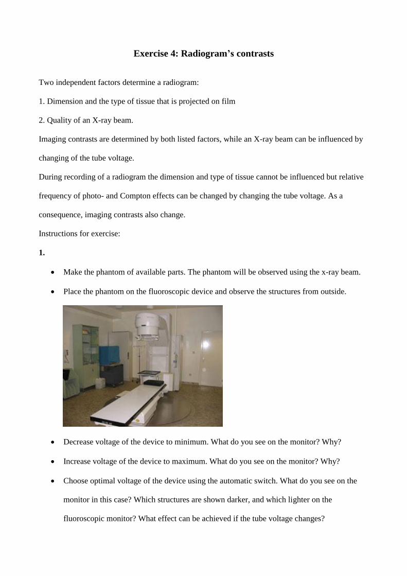
Make the phantom of available parts. The phantom will be observed using the x-ray beam.
Place the phantom on the fluoroscopic device and observe the structures from outside.
Decrease voltage of the device to minimum. What do you see on the monitor? Why?
Increase voltage of the device to maximum. What do you see on the monitor? Why?
Choose optimal voltage of the device using the automatic switch. What do you see on the
monitor in this case? Which structures are shown darker, and which lighter on the
fluoroscopic monitor? What effect can be achieved if the tube voltage changes?
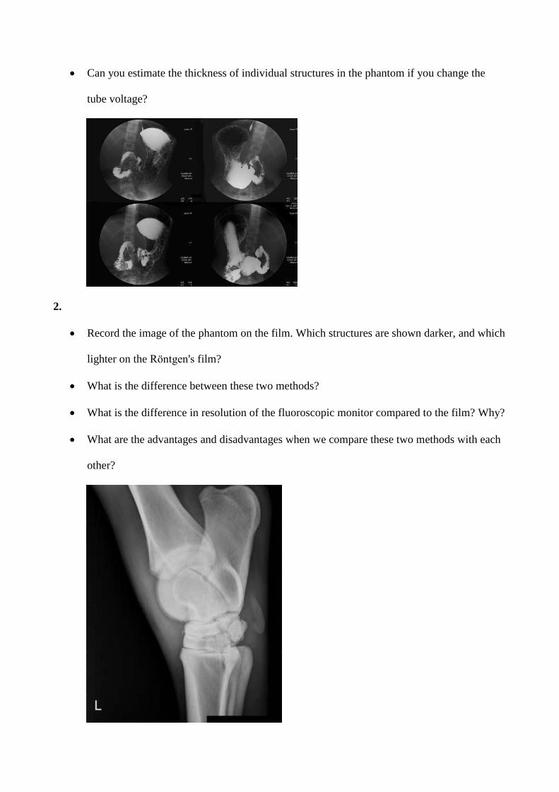
Can you estimate the thickness of individual structures in the phantom if you change the
tube voltage?
2.
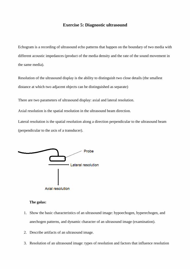
Record the image of the phantom on the film. Which structures are shown darker, and which
lighter on the Röntgen's film?
What is the difference between these two methods?
What is the difference in resolution of the fluoroscopic monitor compared to the film? Why?
What are the advantages and disadvantages when we compare these two methods with each
other?
Exercise 5: Diagnostic ultrasound
Echogram is a recording of ultrasound echo patterns that happen on the boundary of two media with
different acoustic impedances (product of the media density and the rate of the sound movement in
the same media).
Resolution of the ultrasound display is the ability to distinguish two close details (the smallest
distance at which two adjacent objects can be distinguished as separate)
There are two parameters of ultrasound display: axial and lateral resolution.
Axial resolution is the spatial resolution in the ultrasound beam direction.
Lateral resolution is the spatial resolution along a direction perpendicular to the ultrasound beam
(perpendicular to the axis of a transducer).
The golas:
1. Show the basic characteristics of an ultrasound image: hypoechogen, hyperechogen, and
anechogen patterns, and dynamic character of an ultrasound image (examination).
2. Describe artifacts of an ultrasound image.
3. Resolution of an ultrasound image: types of resolution and factors that influence resolution
Instructions for exercise:
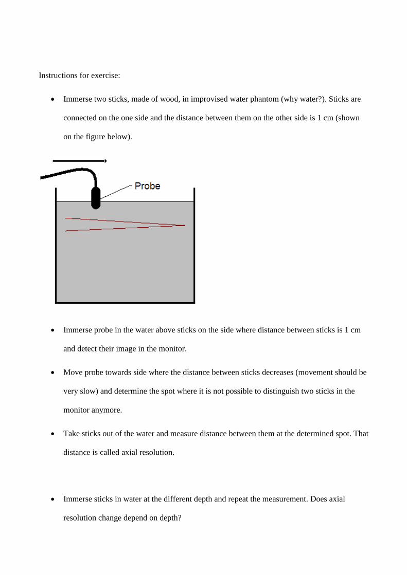
Immerse two sticks, made of wood, in improvised water phantom (why water?). Sticks are
connected on the one side and the distance between them on the other side is 1 cm (shown
on the figure below).
Immerse probe in the water above sticks on the side where distance between sticks is 1 cm
and detect their image in the monitor.
Move probe towards side where the distance between sticks decreases (movement should be
very slow) and determine the spot where it is not possible to distinguish two sticks in the
monitor anymore.
Take sticks out of the water and measure distance between them at the determined spot. That
distance is called axial resolution.
Immerse sticks in water at the different depth and repeat the measurement. Does axial
resolution change depend on depth?

Rotate sticks for a 90º and immerse it again in the water at the same depth like at the
beginning. That will allow you to measure lateral resolution.
Repeat the procedure described for axial resolution again. How does image of sticks look
like in the monitor at the beginning?
When you determine the spot where it is not possible to distinguish images of two sticks in
the monitor anymore take the sticks out of the water and measure distance between them at
the determined spot. That distance is called lateral resolution. What is the difference
between axial and lateral resolution? What causes that difference?
Immerse a metal ball in the water, respectively, and find its image in the monitor. Describe
the image. What artifact do you see?
Repeat the same with a prepared glove.
Exercise 6: Neural signal
Hodgkin Huxley model of propagation of action potentials
In 1952, Hodgkin and Huxley published seminal scientific paper that describes initiation and
propagation of action potential as a function of ionic conductivity of membrane channels in the
nerve cells. Their contribution to the understanding of neural signal propagation is awarded with the
Nobel Prize in physiology and medicine in 1964.
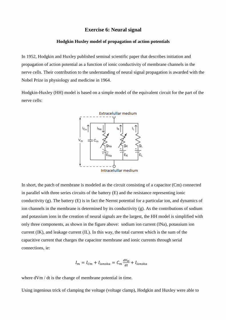
Hodgkin-Huxley (HH) model is based on a simple model of the equivalent circuit for the part of the
nerve cells:
In short, the patch of membrane is modeled as the circuit consisting of a capacitor (Cm) connected
in parallel with three series circuits of the battery (E) and the resistance representing ionic
conductivity (g). The battery (E) is in fact the Nernst potential for a particular ion, and dynamics of
ion channels in the membrane is determined by its conductivity (g). As the contributions of sodium
and potassium ions in the creation of neural signals are the largest, the HH model is simplified with
only three components, as shown in the figure above: sodium ion current (INa), potassium ion
current (IK), and leakage current (IL). In this way, the total current which is the sum of the
capacitive current that charges the capacitor membrane and ionic currents through serial
connections, ie:
where dVm / dt is the change of membrane potential in time.
Using ingenious trick of clamping the voltage (voltage clamp), Hodgkin and Huxley were able to
separate the ionic currents from the capacitor’s current in order to determine the contribution of
ionic currents. This was done in the squid axon which is quite large and therefore relatively easy to
experiment with. In the next step, using voltage and current clamp, H&H were able to separate
ionic currents of each ion, showing them that the ionic currents of sodium and potassium follow the
Ohm's law (I = V / R). Thus, the ionic current of each membrane channel is proportional to its
conductivity (i.e, inversely proportional to the resistance) and to the potential difference for the
ionic channel, i.e.:
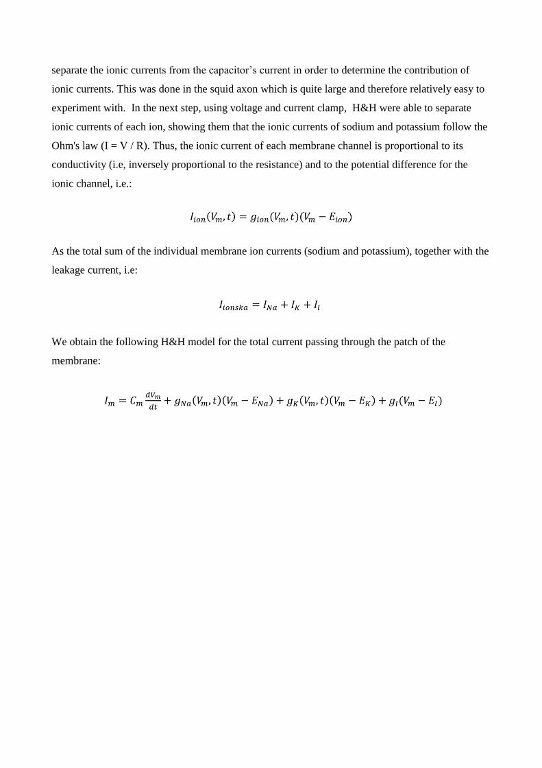
As the total sum of the individual membrane ion currents (sodium and potassium), together with the
leakage current, i.e:
We obtain the following H&H model for the total current passing through the patch of the
membrane:
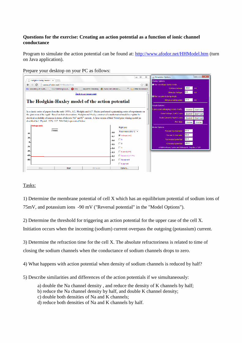
Questions for the exercise: Creating an action potential as a function of ionic channel
conductance
Program to simulate the action potential can be found at: http://www.afodor.net/HHModel.htm (turn
on Java application).
Prepare your desktop on your PC as follows:
Tasks:
1) Determine the membrane potential of cell X which has an equilibrium potential of sodium ions of
75mV, and potassium ions -90 mV ("Reversal potential" in the "Model Options").
2) Determine the threshold for triggering an action potential for the upper case of the cell X.
Initiation occurs when the incoming (sodium) current overpass the outgoing (potassium) current.
3) Determine the refraction time for the cell X. The absolute refractoriness is related to time of
closing the sodium channels when the conductance of sodium channels drops to zero.
4) What happens with action potential when density of sodium channels is reduced by half?
5) Describe similarities and differences of the action potentials if we simultaneously:
a) double the Na channel density , and reduce the density of K channels by half;
b) reduce the Na channel density by half, and double K channel density;
c) double both densities of Na and K channels;
d) reduce both densities of Na and K channels by half.
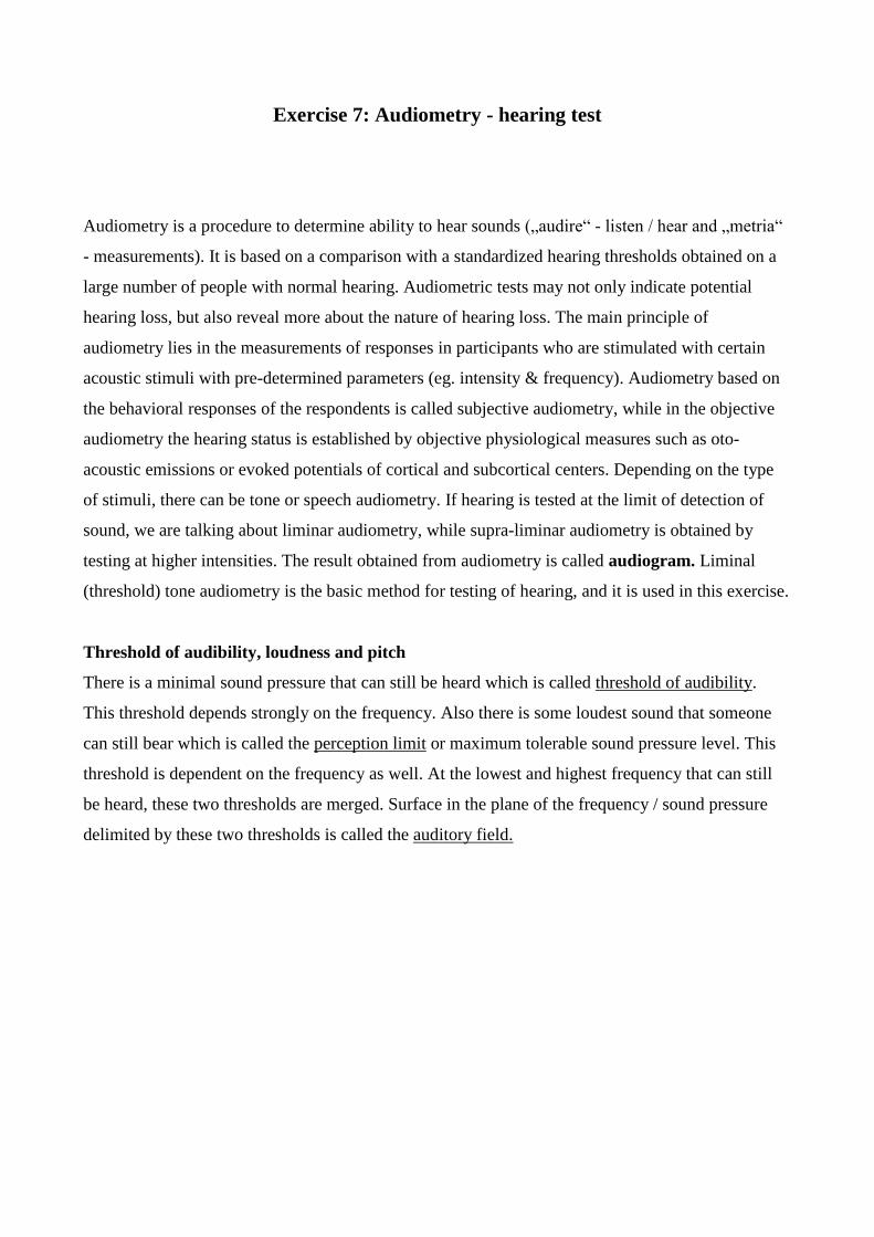
Exercise 7: Audiometry - hearing test
Audiometry is a procedure to determine ability to hear sounds („audire“ - listen / hear and „metria“
- measurements). It is based on a comparison with a standardized hearing thresholds obtained on a
large number of people with normal hearing. Audiometric tests may not only indicate potential
hearing loss, but also reveal more about the nature of hearing loss. The main principle of
audiometry lies in the measurements of responses in participants who are stimulated with certain
acoustic stimuli with pre-determined parameters (eg. intensity & frequency). Audiometry based on
the behavioral responses of the respondents is called subjective audiometry, while in the objective
audiometry the hearing status is established by objective physiological measures such as oto-
acoustic emissions or evoked potentials of cortical and subcortical centers. Depending on the type
of stimuli, there can be tone or speech audiometry. If hearing is tested at the limit of detection of
sound, we are talking about liminar audiometry, while supra-liminar audiometry is obtained by
testing at higher intensities. The result obtained from audiometry is called audiogram. Liminal
(threshold) tone audiometry is the basic method for testing of hearing, and it is used in this exercise.
Threshold of audibility, loudness and pitch
There is a minimal sound pressure that can still be heard which is called threshold of audibility.
This threshold depends strongly on the frequency. Also there is some loudest sound that someone
can still bear which is called the perception limit or maximum tolerable sound pressure level. This
threshold is dependent on the frequency as well. At the lowest and highest frequency that can still
be heard, these two thresholds are merged. Surface in the plane of the frequency / sound pressure
delimited by these two thresholds is called the auditory field.
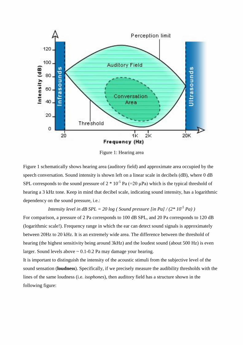
Figure 1: Hearing area
Figure 1 schematically shows hearing area (auditory field) and approximate area occupied by the
speech conversation. Sound intensity is shown left on a linear scale in decibels (dB), where 0 dB
SPL corresponds to the sound pressure of 2 * 10-5
Pa (=20 µPa) which is the typical threshold of
hearing a 3 kHz tone. Keep in mind that decibel scale, indicating sound intensity, has a logarithmic
dependency on the sound pressure, i.e.:
Intensity level in dB SPL = 20 log ( Sound pressure [in Pa] / (2* 10-5
Pa) )
For comparison, a pressure of 2 Pa corresponds to 100 dB SPL, and 20 Pa corresponds to 120 dB
(logarithmic scale!). Frequency range in which the ear can detect sound signals is approximately
between 20Hz to 20 kHz. It is an extremely wide area. The difference between the threshold of
hearing (the highest sensitivity being around 3kHz) and the loudest sound (about 500 Hz) is even
larger. Sound levels above ~ 0.1-0.2 Pa may damage your hearing.
It is important to distinguish the intensity of the acoustic stimuli from the subjective level of the
sound sensation (loudness). Specifically, if we precisely measure the audibility thresholds with the
lines of the same loudness (i.e. isophones), then auditory field has a structure shown in the
following figure:
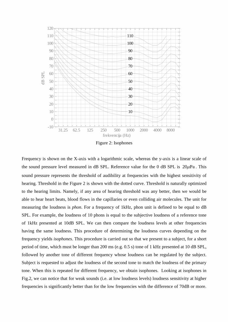
Figure 2: Isophones
Frequency is shown on the X-axis with a logarithmic scale, whereas the y-axis is a linear scale of
the sound pressure level measured in dB SPL. Reference value for the 0 dB SPL is Pa20 . This
sound pressure represents the threshold of audibility at frequencies with the highest sensitivity of
hearing. Threshold in the Figure 2 is shown with the dotted curve. Threshold is naturally optimized
to the hearing limits. Namely, if any area of hearing threshold was any better, then we would be
able to hear heart beats, blood flows in the capillaries or even colliding air molecules. The unit for
measuring the loudness is phon. For a frequency of 1kHz, phon unit is defined to be equal to dB
SPL. For example, the loudness of 10 phons is equal to the subjective loudness of a reference tone
of 1kHz presented at 10dB SPL. We can then compare the loudness levels at other frequencies
having the same loudness. This procedure of determining the loudness curves depending on the
frequency yields isophones. This procedure is carried out so that we present to a subject, for a short
period of time, which must be longer than 200 ms (e.g. 0.5 s) tone of 1 kHz presented at 10 dB SPL,
followed by another tone of different frequency whose loudness can be regulated by the subject.
Subject is requested to adjust the loudness of the second tone to match the loudness of the primary
tone. When this is repeated for different frequency, we obtain isophones. Looking at isophones in
Fig.2, we can notice that for weak sounds (i.e. at low loudness levels) loudness sensitivity at higher
frequencies is significantly better than for the low frequencies with the difference of 70dB or more.
31.25 62.5 125 250 500 1000 2000 4000 8000-10
0
10
20
30
40
50
60
70
80
90
100
110
120
10
20
30
40
50
60
70
80
90
100
110
frekvencija (Hz)
dB
SP
L
izofone
If the loudness increases, then the "frequency response" of isophones becomes more linear, so in the
example of 100-phone isophone, such difference is less than 30 dB. This means that sound pressure
does not contribute equally at low and high frequencies. This can explain why rock concerts sound
good if they are loud, and quiet recordings sound "empty" because they have essentially reduced
low, and to some degree high frequencies. Therefore, the ear is very nonlinear converter.
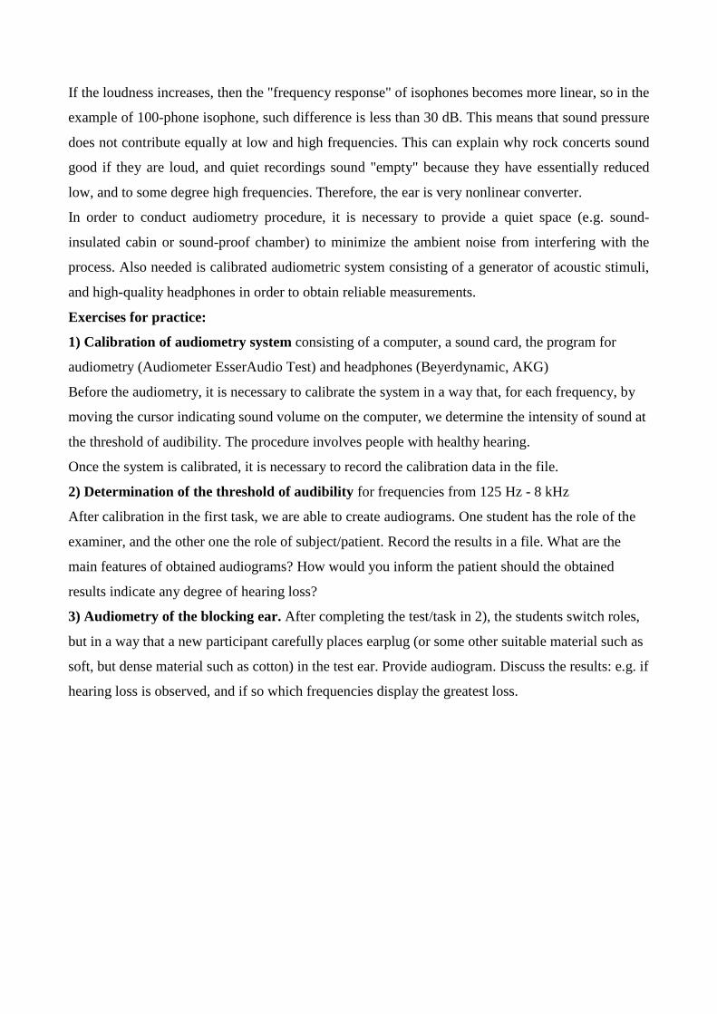
In order to conduct audiometry procedure, it is necessary to provide a quiet space (e.g. sound-
insulated cabin or sound-proof chamber) to minimize the ambient noise from interfering with the
process. Also needed is calibrated audiometric system consisting of a generator of acoustic stimuli,
and high-quality headphones in order to obtain reliable measurements.
Exercises for practice:
1) Calibration of audiometry system consisting of a computer, a sound card, the program for
audiometry (Audiometer EsserAudio Test) and headphones (Beyerdynamic, AKG)
Before the audiometry, it is necessary to calibrate the system in a way that, for each frequency, by
moving the cursor indicating sound volume on the computer, we determine the intensity of sound at
the threshold of audibility. The procedure involves people with healthy hearing.
Once the system is calibrated, it is necessary to record the calibration data in the file.
2) Determination of the threshold of audibility for frequencies from 125 Hz - 8 kHz
After calibration in the first task, we are able to create audiograms. One student has the role of the
examiner, and the other one the role of subject/patient. Record the results in a file. What are the
main features of obtained audiograms? How would you inform the patient should the obtained
results indicate any degree of hearing loss?
3) Audiometry of the blocking ear. After completing the test/task in 2), the students switch roles,
but in a way that a new participant carefully places earplug (or some other suitable material such as
soft, but dense material such as cotton) in the test ear. Provide audiogram. Discuss the results: e.g. if
hearing loss is observed, and if so which frequencies display the greatest loss.
Exercise 8: Optical bench
Converging lenses
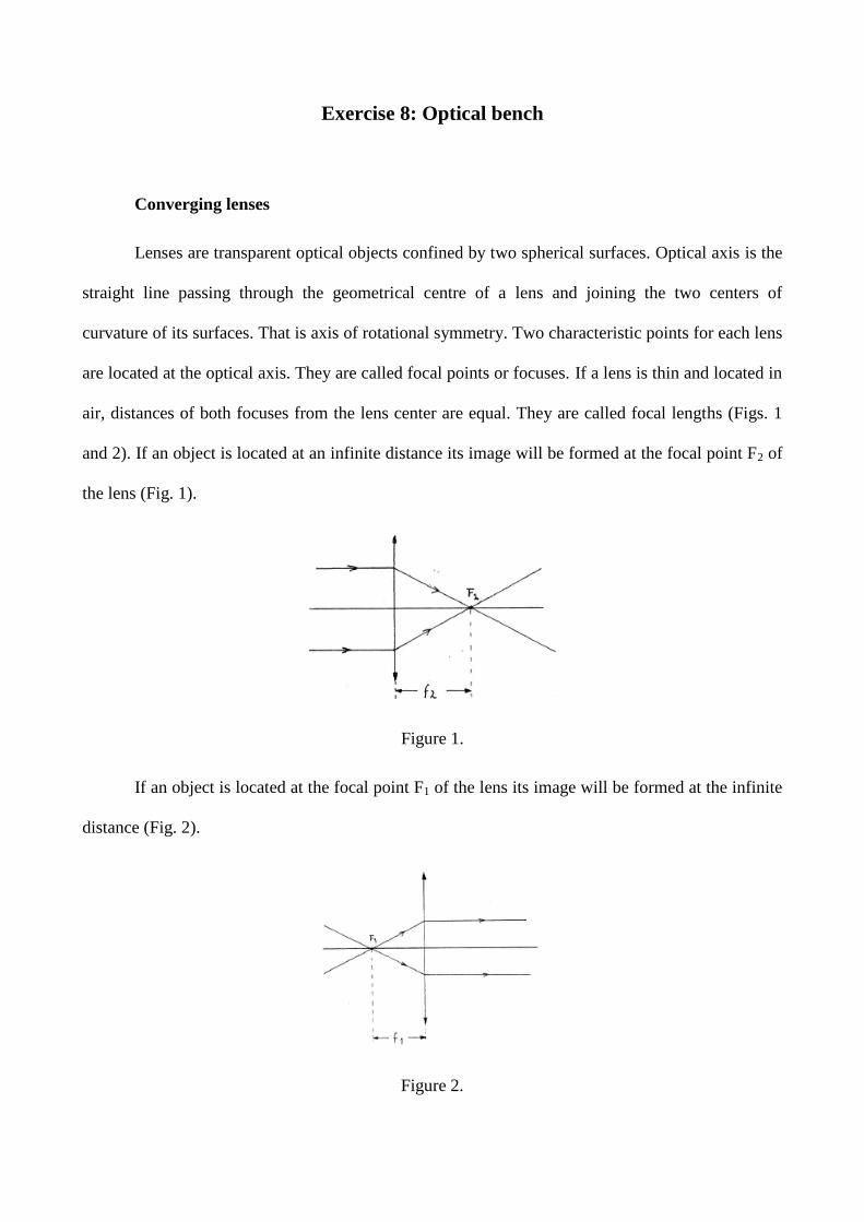
Lenses are transparent optical objects confined by two spherical surfaces. Optical axis is the
straight line passing through the geometrical centre of a lens and joining the two centers of
curvature of its surfaces. That is axis of rotational symmetry. Two characteristic points for each lens
are located at the optical axis. They are called focal points or focuses. If a lens is thin and located in
air, distances of both focuses from the lens center are equal. They are called focal lengths (Figs. 1
and 2). If an object is located at an infinite distance its image will be formed at the focal point F2 of
the lens (Fig. 1).
Figure 1.
If an object is located at the focal point F1 of the lens its image will be formed at the infinite
distance (Fig. 2).
Figure 2.
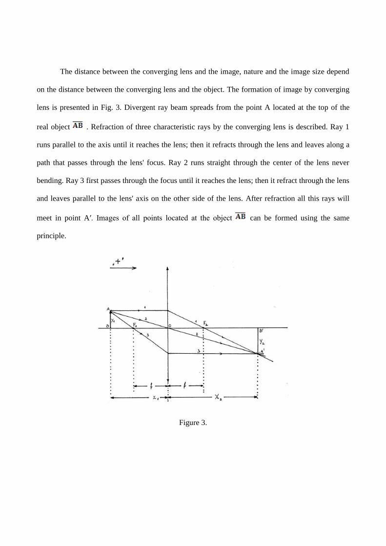
The distance between the converging lens and the image, nature and the image size depend
on the distance between the converging lens and the object. The formation of image by converging
lens is presented in Fig. 3. Divergent ray beam spreads from the point A located at the top of the
real object . Refraction of three characteristic rays by the converging lens is described. Ray 1
runs parallel to the axis until it reaches the lens; then it refracts through the lens and leaves along a
path that passes through the lens' focus. Ray 2 runs straight through the center of the lens never
bending. Ray 3 first passes through the focus until it reaches the lens; then it refract through the lens
and leaves parallel to the lens' axis on the other side of the lens. After refraction all this rays will
meet in point A′. Images of all points located at the object can be formed using the same
principle.
Figure 3.
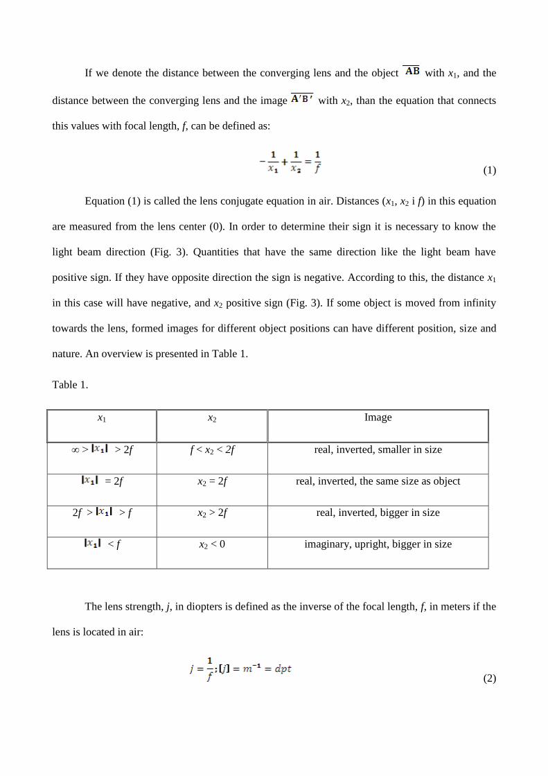
If we denote the distance between the converging lens and the object with x1, and the
distance between the converging lens and the image with x2, than the equation that connects
this values with focal length, f, can be defined as:
(1)
Equation (1) is called the lens conjugate equation in air. Distances (x1, x2 i f) in this equation
are measured from the lens center (0). In order to determine their sign it is necessary to know the
light beam direction (Fig. 3). Quantities that have the same direction like the light beam have
positive sign. If they have opposite direction the sign is negative. According to this, the distance x1
in this case will have negative, and x2 positive sign (Fig. 3). If some object is moved from infinity
towards the lens, formed images for different object positions can have different position, size and
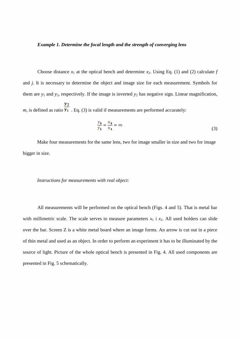
nature. An overview is presented in Table 1.
Table 1.
x1 x2 Image
∞ > > 2f f < x2 < 2f real, inverted, smaller in size
= 2f x2 = 2f real, inverted, the same size as object
2f > > f x2 > 2f real, inverted, bigger in size
< f x2 < 0 imaginary, upright, bigger in size
The lens strength, j, in diopters is defined as the inverse of the focal length, f, in meters if the
lens is located in air:
(2)
Example 1. Determine the focal length and the strength of converging lens
Choose distance x1 at the optical bench and determine x2. Using Eq. (1) and (2) calculate f
and j. It is necessary to determine the object and image size for each measurement. Symbols for
them are y1 and y2, respectively. If the image is inverted y2 has negative sign. Linear magnification,
m, is defined as ratio . Eq. (3) is valid if measurements are performed accurately:
(3)
Make four measurements for the same lens, two for image smaller in size and two for image
bigger in size.
Instructions for measurements with real object:
All measurements will be performed on the optical bench (Figs. 4 and 5). That is metal bar
with millimetric scale. The scale serves to measure parameters x1 i x2. All used holders can slide
over the bar. Screen Z is a white metal board where an image forms. An arrow is cut out in a piece
of thin metal and used as an object. In order to perform an experiment it has to be illuminated by the
source of light. Picture of the whole optical bench is presented in Fig. 4. All used components are
presented in Fig. 5 schematically.
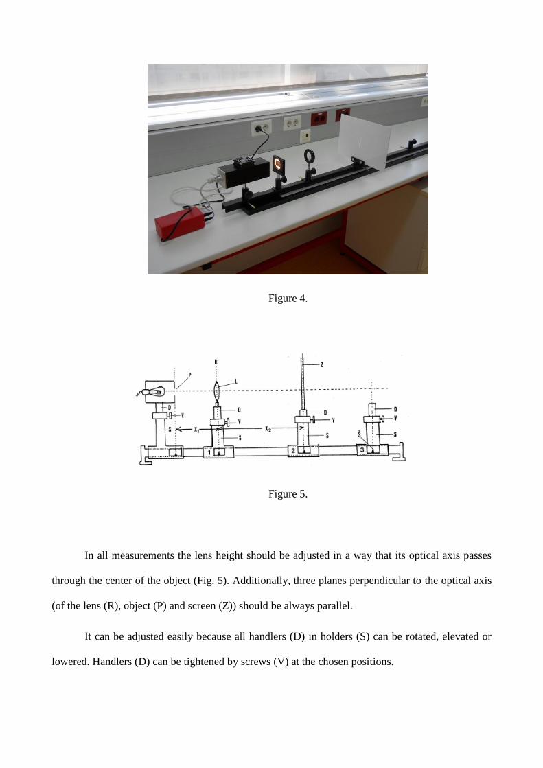
Figure 4.
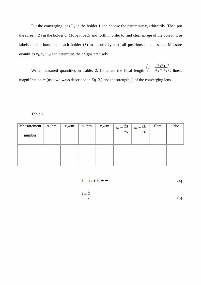
Figure 5.
In all measurements the lens height should be adjusted in a way that its optical axis passes
through the center of the object (Fig. 5). Additionally, three planes perpendicular to the optical axis
(of the lens (R), object (P) and screen (Z)) should be always parallel.
It can be adjusted easily because all handlers (D) in holders (S) can be rotated, elevated or
lowered. Handlers (D) can be tightened by screws (V) at the chosen positions.
Put the converging lens Lk in the holder 1 and choose the parameter x1 arbitrarily. Then put
the screen (Z) in the holder 2. Move it back and forth in order to find clear image of the object. Use
labels on the bottom of each holder (S) to accurately read all positions on the scale. Measure
quantities x1, x2 i y2 and determine their signs precisely.
Write measured quantities in Table. 2. Calculate the focal length , linear
magnification m (use two ways described in Eq. 3.) and the strength, j, of the converging lens.
Table 2.
Measurement
number
x1/cm x2/cm y1/cm y2/cm
f/cm j/dpt
(4)
(5)
Example 2. Determine the focal length and the strength of converging lens using method
of virtual object
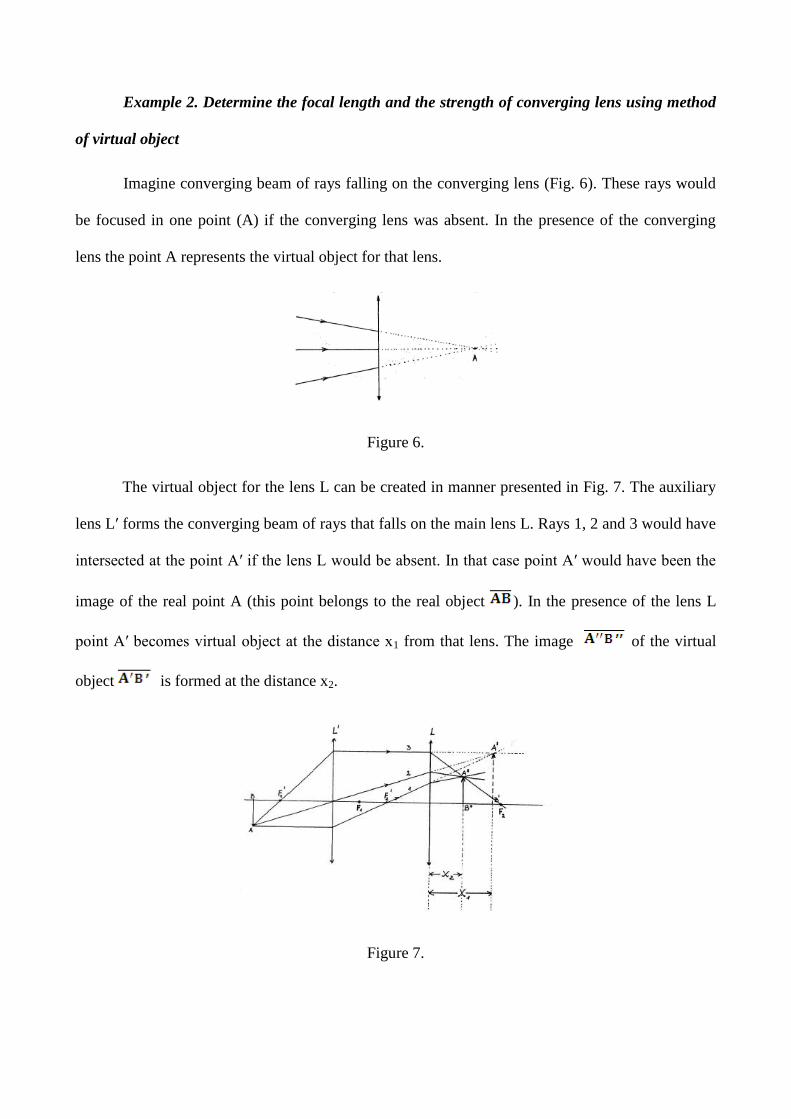
Imagine converging beam of rays falling on the converging lens (Fig. 6). These rays would
be focused in one point (A) if the converging lens was absent. In the presence of the converging
lens the point A represents the virtual object for that lens.
Figure 6.
The virtual object for the lens L can be created in manner presented in Fig. 7. The auxiliary
lens L′ forms the converging beam of rays that falls on the main lens L. Rays 1, 2 and 3 would have
intersected at the point A′ if the lens L would be absent. In that case point A′ would have been the
image of the real point A (this point belongs to the real object ). In the presence of the lens L
point A′ becomes virtual object at the distance x1 from that lens. The image of the virtual
object is formed at the distance x2.
Figure 7.
Quantities x1 i x2 in this example, according to previously described rule, have positive
signs.
Instructions for measurements with virtual object:
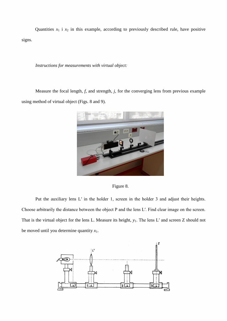
Measure the focal length, f, and strength, j, for the converging lens from previous example
using method of virtual object (Figs. 8 and 9).
Figure 8.
Put the auxiliary lens L′ in the holder 1, screen in the holder 3 and adjust their heights.
Choose arbitrarily the distance between the object P and the lens L′. Find clear image on the screen.
That is the virtual object for the lens L. Measure its height, y1. The lens L′ and screen Z should not
be moved until you determine quantity x1.
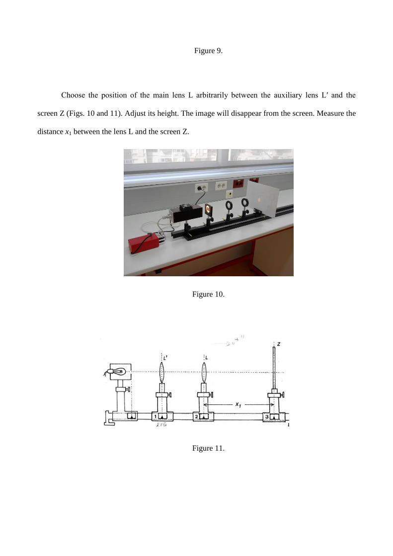
Figure 9.
Choose the position of the main lens L arbitrarily between the auxiliary lens L′ and the
screen Z (Figs. 10 and 11). Adjust its height. The image will disappear from the screen. Measure the
distance x1 between the lens L and the screen Z.
Figure 10.
Figure 11.
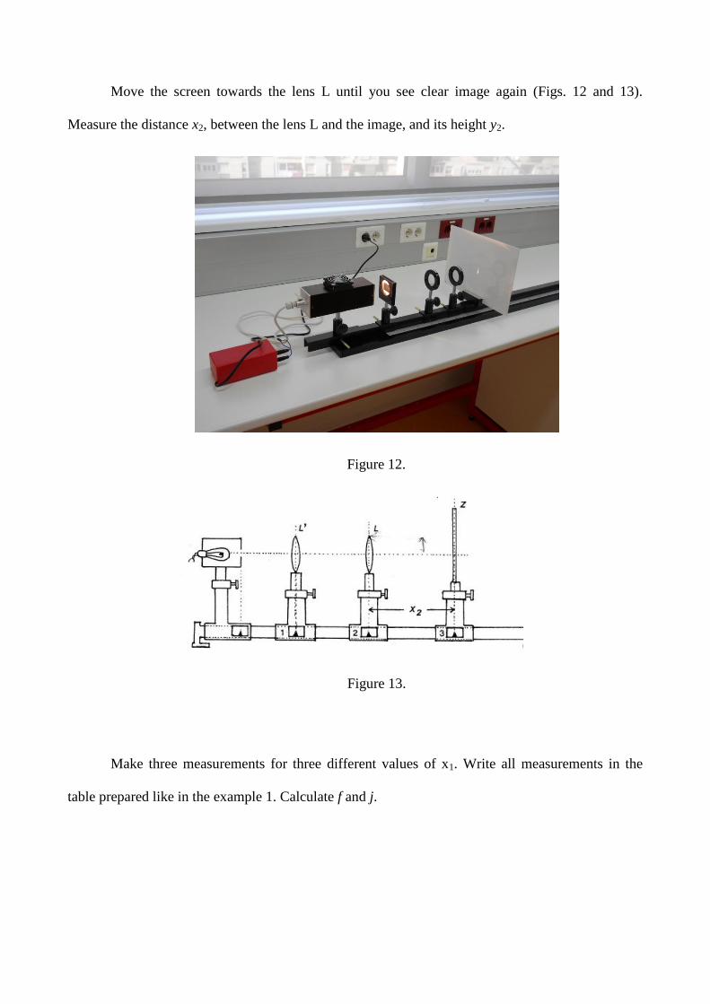
Move the screen towards the lens L until you see clear image again (Figs. 12 and 13).
Measure the distance x2, between the lens L and the image, and its height y2.
Figure 12.
Figure 13.
Make three measurements for three different values of x1. Write all measurements in the
table prepared like in the example 1. Calculate f and j.
Example 3. Determine the focal length and the strength of converging lens using Bessel’s
method
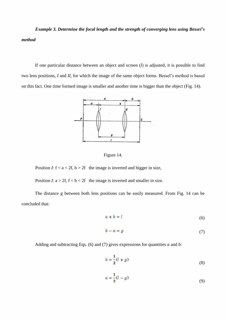
If one particular distance between an object and screen (l) is adjusted, it is possible to find
two lens positions, I and II, for which the image of the same object forms. Bessel’s method is based
on this fact. One time formed image is smaller and another time is bigger than the object (Fig. 14).
Figure 14.
Position I: f < a < 2f, b > 2f the image is inverted and bigger in size,
Position I: a > 2f, f < b < 2f the image is inverted and smaller in size.
The distance g between both lens positions can be easily measured. From Fig. 14 can be
concluded that:
(6)
(7)
Adding and subtracting Eqs. (6) and (7) gives expressions for quantities a and b:
(8)
(9)
Combining Eqs. (8) i (9) with Eq (1) give an expression for focal length:
(10)
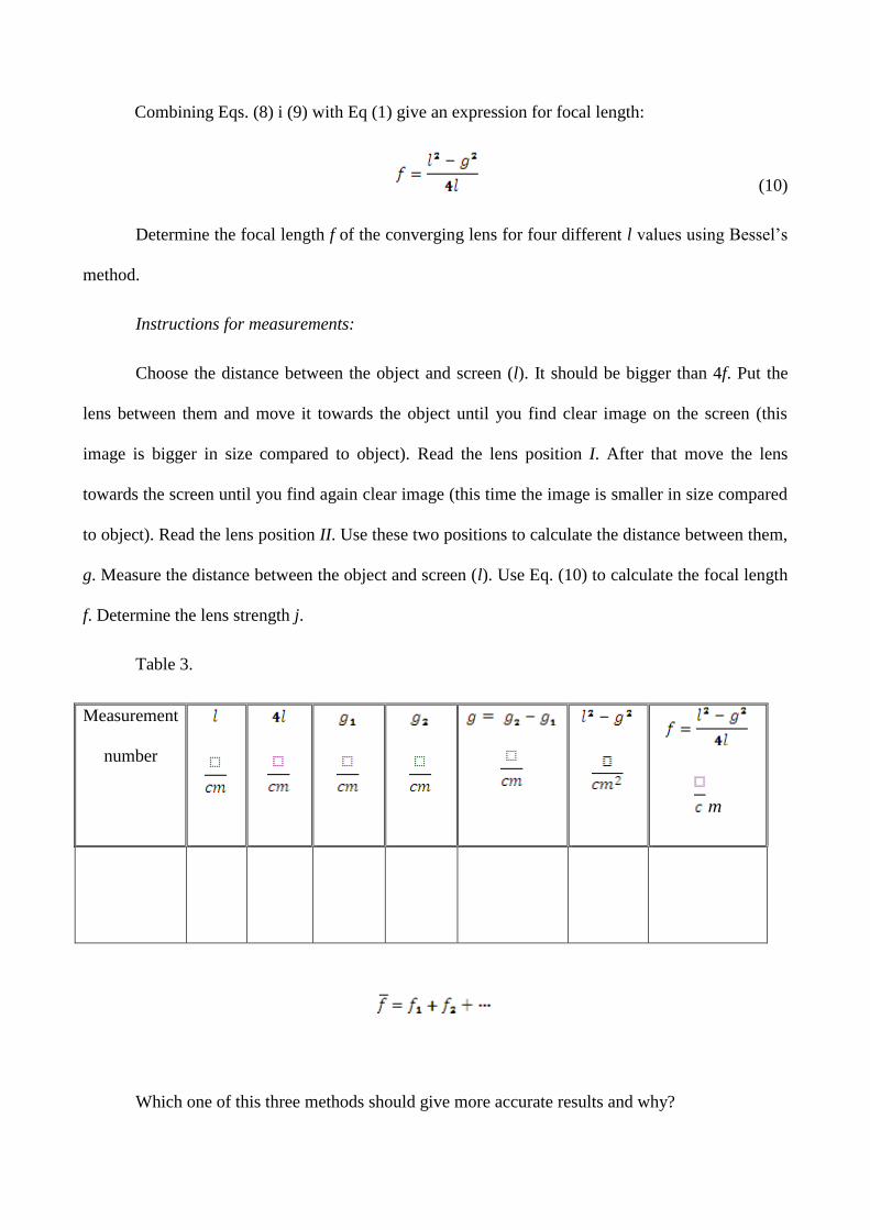
Determine the focal length f of the converging lens for four different l values using Bessel’s
method.
Instructions for measurements:
Choose the distance between the object and screen (l). It should be bigger than 4f. Put the
lens between them and move it towards the object until you find clear image on the screen (this
image is bigger in size compared to object). Read the lens position I. After that move the lens
towards the screen until you find again clear image (this time the image is smaller in size compared
to object). Read the lens position II. Use these two positions to calculate the distance between them,
g. Measure the distance between the object and screen (l). Use Eq. (10) to calculate the focal length
f. Determine the lens strength j.
Table 3.
Measurement
number
m
Which one of this three methods should give more accurate results and why?
Exercise 9: Viscosity of fluids
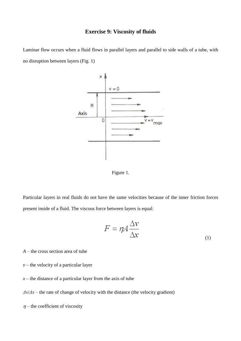
Laminar flow occurs when a fluid flows in parallel layers and parallel to side walls of a tube, with
no disruption between layers (Fig. 1)
Figure 1.
Particular layers in real fluids do not have the same velocities because of the inner friction forces
present inside of a fluid. The viscous force between layers is equal:
(1)
A – the cross section area of tube
v – the velocity of a particular layer
x – the distance of a particular layer from the axis of tube
Δv/Δx – the rate of change of velocity with the distance (the velocity gradient)
– the coefficient of viscosity
It is possible to determine the unit for the coefficient of viscosity from equation (1):
(2)
Layers of a fluid located immediately by the side wall of tube are at rest, v(R)=0, while the layer
whose flow coincide with axis has maximal velocity, v(0)=vmax. Distribution of velocities of all
layers is parabolic function. It depends on parameter x (the distance of a particular layer from the
axis of tube):
(3)
Newtonian fluids are real fluids in which viscosity is independent on volume flow rate at certain
temperature. Volume, V, of such fluid can be calculated according to Poiseuille’s law:
(4)
r – the radius of tube
Δp – the pressure difference between the ends
t – time
– the coefficient of viscosity
l – the length of tube
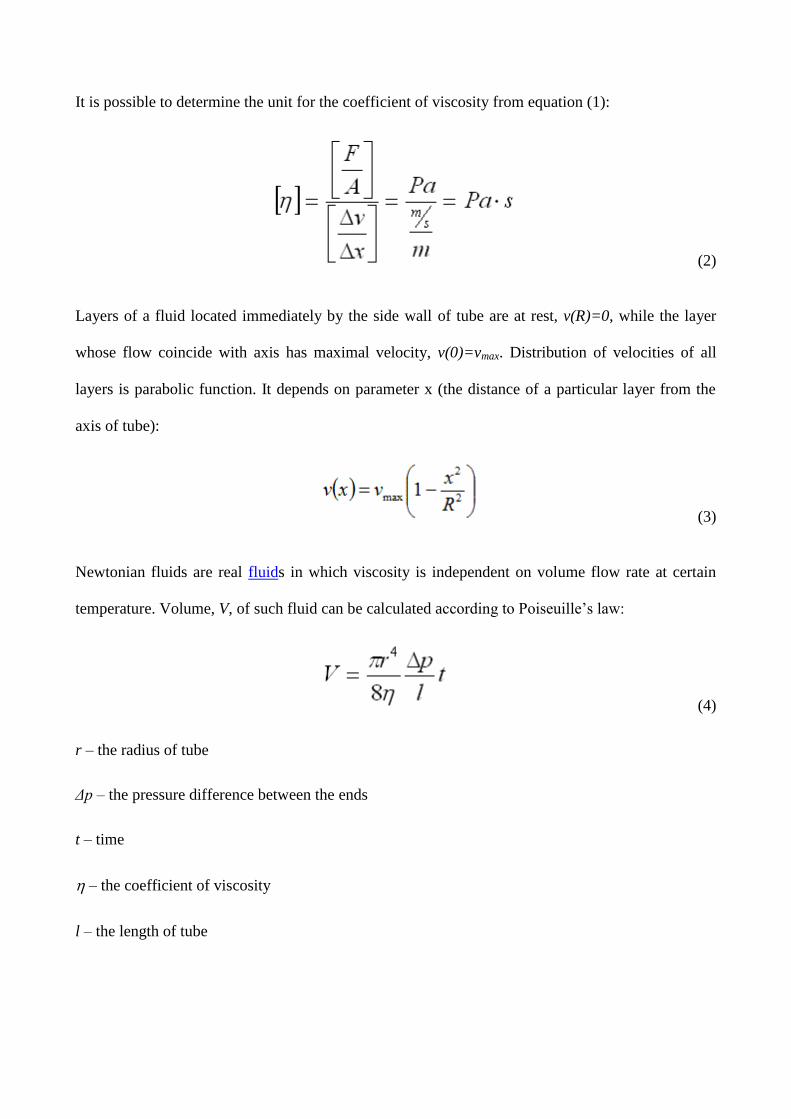
Instructions for exercise:
In this exercise we measure the relative viscosity of unknown fluid and water. Ostwald viscometer,
shown in Fig. 2, is used. Ostwald viscometer is U tube made of glass and has two unequal arms.
Fluid has to be poured in the broader arm. Reservoir of volume V is located close to the top of the
narrower arm. It is confined between labels a and b. We will measure a time required for water or
fluid level to descend between labels a and b; i.e. time required to elapse volume V of certain fluid.
Figure 2.
Using Eq. (4) it is possible to determine the coefficient of viscosity of unknown fluid, ηt. It is
necessary to use equal volumes of water and unknown fluid in all measurements. Based on this we
can use following equations:
(5)
The pressure difference between the ends can be determined using Eq. (6):
(6)
If we combine equations (5) and (6) the formula for the relative viscosity can be derived:
(7)
Or:
(8)
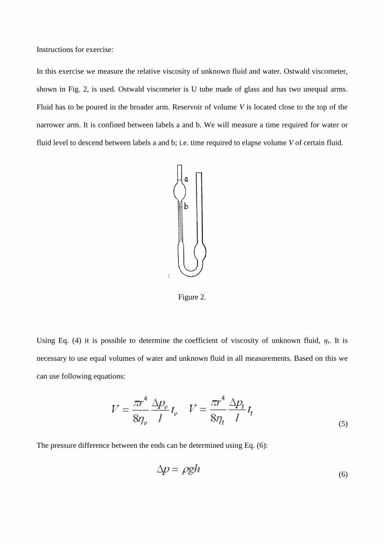
Example 1. Determine the relative viscosity of unknown fluid compared to water using Ostwald
viscometer
The density of an unknown fluid is written on the bottle. Take 10 ml of water using a pipette and
pour it in the broader arm of the viscometer. Elevate water level in the narrower arm above the label
a. Let water to flow. Turn on a stop-watch at the moment when the water level elapses by label a
and turn it off when it elapses by label b. Repeat the same measurement a few times. The next step
is to empty the viscometer and rinse it with few milliliters of unknown fluid. Repeat the same
measurements with 10 ml of an unknown fluid a few times. Write all results in table 1.
Table 1.
Measurement
number
Water Fluid
tv (s) Δtv (s) tt (s) Δtt (s)
Based on this data calculate the relative viscosity using Eq. (8)
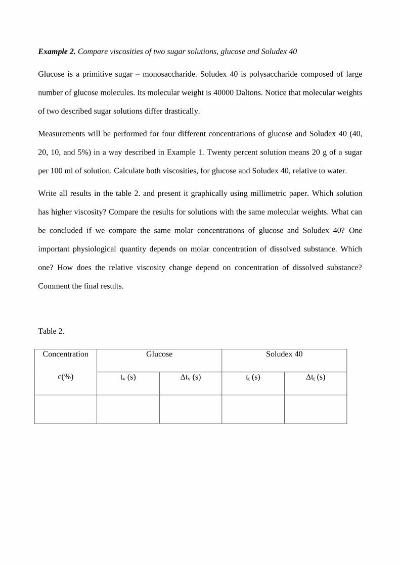
Example 2. Compare viscosities of two sugar solutions, glucose and Soludex 40
Glucose is a primitive sugar – monosaccharide. Soludex 40 is polysaccharide composed of large
number of glucose molecules. Its molecular weight is 40000 Daltons. Notice that molecular weights
of two described sugar solutions differ drastically.
Measurements will be performed for four different concentrations of glucose and Soludex 40 (40,
20, 10, and 5%) in a way described in Example 1. Twenty percent solution means 20 g of a sugar
per 100 ml of solution. Calculate both viscosities, for glucose and Soludex 40, relative to water.
Write all results in the table 2. and present it graphically using millimetric paper. Which solution
has higher viscosity? Compare the results for solutions with the same molecular weights. What can
be concluded if we compare the same molar concentrations of glucose and Soludex 40? One
important physiological quantity depends on molar concentration of dissolved substance. Which
one? How does the relative viscosity change depend on concentration of dissolved substance?
Comment the final results.
Table 2.
Concentration
c(%)
Glucose Soludex 40
tv (s) Δtv (s) tt (s) Δtt (s)

0 20 40 60 80 1000
2
4
6
re
l
c (%)
Graph 1.
Example 3. Repeat all measurements using solution from Example 1. at different temperatures.
Present graphically the dependence of viscosity on temperature and comment the final result.
Exercise 10: Hemodynamics
Goals:
Illustration of basic hemorheologic laws: (i) proportionality between the arterial pressure and
blood flow and (ii) approximate proportionality between the left ventricular stroke volume and
pulse pressure (difference between systolic and diastolic pressure),
demonstration of a possibility to noninvasively assess the hemorheologic parameters, instead of a
complex and invasive direct measurement,
illustration of a modeling in medicine, when one uses reasonable approximations to relate the
physiologic parameters with quantities that can be measured simply and accurately,
gaining an insight in practical problems of measuring the arterial pressure and heart rate at rest
and during exercise, as well as in measurement errors and ways to assess these errors.
BACKGROUND
This exercise shows and quantitatively assess that the total peripheral resistance (R) decreases
during aerobic exercise, the more the level of exercise is.
One uses the approximate proportionality of the left ventricular stroke volume (SV) and pulse
pressure; a difference between systolic pressure Ps and diastolic pressure, Pd; P=Ps-Pd.
The left ventricle ejects the majority of its stroke volume (about 80%) in the first third of systole,
during the fast ejection phase. During this time the pressure increases from minimal (diastolic) to
maximal (systolic) value, which enlarges the aorta from minimal to maximal volume, depending on
its compliance (Caorta ). Within bounds of elastic proportionality the systolic increase in aortic
volume is:
systolic increase in aortic volume = P x Caorta (1)
The systolic increase in aortic volume is less than its stroke volume because (i) the volume of blood
ejected in the period of fast ejection is only 80% and (ii) some of this output leaves aorta and pushes
the blood through capillaries. Since the peripheral perfusion is nearly constant, the later part,
corresponding to 1/3 of a systole, which itself is 1/3 of a cycle at rest, is thus only about 1/9 of a
stroke volume. Thus:
systolic increase in aortic volume = SV x k (2)
where, roughly, the parameter k is 0.8 x 0.89 0.7.
Combining equations (1) i (2):
P = SV x k/Caorta (3)
Equation (3) expresses the proportionality between pulse pressure and left ventricular stroke volume
(normally it is also the stroke volume of the right heart!). The proportionality constant is the part of
the systolic increase in aortic volume in stroke volume, divided by aortic compliance. In other
words, the greater the stroke volume the greater the pulse pressure, which increases with intensity
of fast ejection and decreases with aortic compliance.
Equation (3) cannot be directly used to assess the stroke volume in a person since aortic compliance
varies between people; in a given person it decreases with age and between different hemodynamic
conditions (it decreases in exercise and other conditions that increase the stroke volume, when
aortic collagen fibers stretch extensively). In addition, the parameter k in equation (3) also depends
on hemodynamic state and decreases in physical stress. In physical stress (and other conditions of
increased cardiac output) the systole occupies larger portion of heart cycle (absolute duration is
fairly constant), so that larger portion of stroke volume goes to periphery during fast ejection (more
than 11%), which itself accounts for less than 80% of stroke volume.
However, applying equation (3) to the same person in two different hemodynamic states, the ratio
of stroke volumes is:
SV1/SV2 = (P1/P2)x(Caorta /k)1/(Caorta /k)2 (4)
Since exercise decreases both parameter k and aortic compliance, it may be reasonable to assume
that their ratio does not change much in the same person between rest and exercise. This is the basic
assumption of our model, enabling us to equate the ratio (Caorte /k)1/(Caorte /k)2 in equation (4) to
unity. This simplifies the equation (4) to:
SV1/SV2 = P1/P2 (5)
Equation (5) enables to assess the exercise induced relative changes in stroke volume from relative
changes in pulse pressure. Since the cardiac output (CO) equals the product of stroke volume and
heart rate (f), equation (5) also gives:
CO1/CO2 = (P1/P2) x (f1/f2) (6)
Equations (5) and (6) relate the quantities that require complex, invasive measurements (stroke
volume, heart output) with quantities accessible simply and noninvasively (systolic and diastolic
blood pressure, heart rate).
Equating the right atrial pressure to zero, the stroke volume equals the mean arterial pressure (Pa)
divided by total peripheral resistance (R):
CO = Pa/R (7)
From relations (6) and (7) it follows that the ratio of peripheral resistances in a person in two
hemodynamic states is:
R1/R2 = (P2/P1)x(f2/f1)xPa1/Pa2 (8)
If indexes 1 and 2 denote stress and rest respectively, the above equation translates to:
Rstress/Rrest = (Prest/Pstress)x(frest/fstress)xPastress/Parest (9)
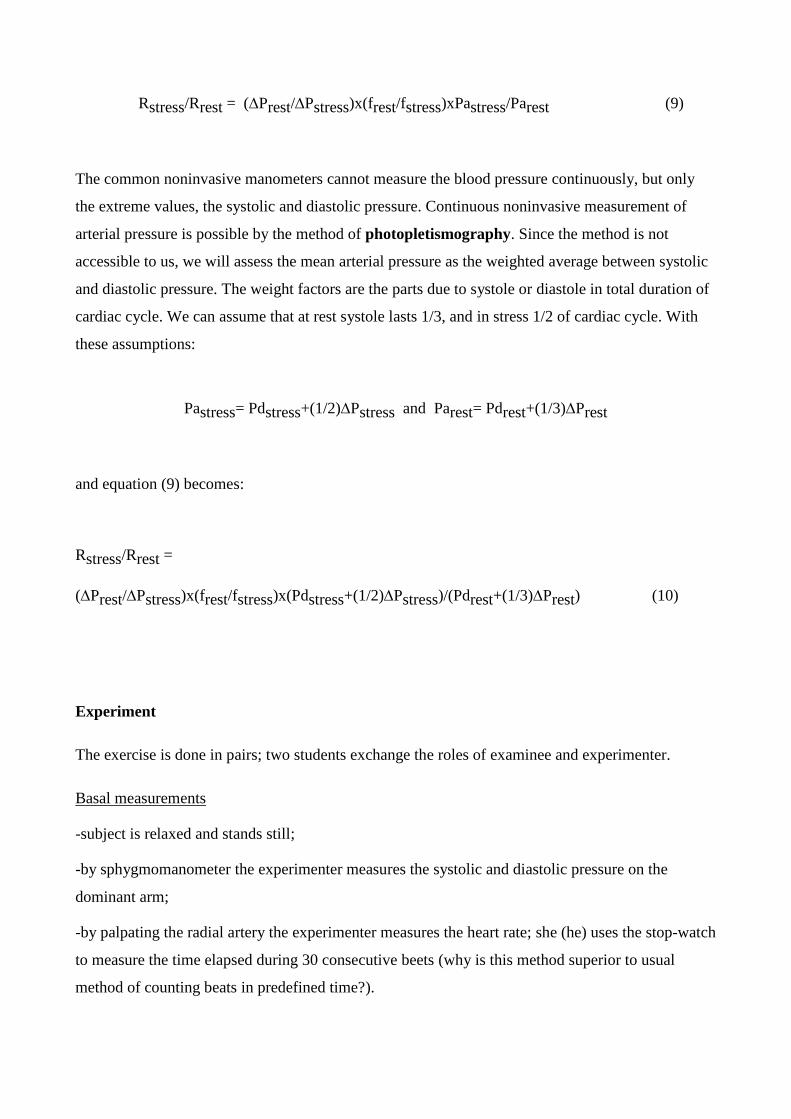
The common noninvasive manometers cannot measure the blood pressure continuously, but only
the extreme values, the systolic and diastolic pressure. Continuous noninvasive measurement of
arterial pressure is possible by the method of photopletismography. Since the method is not
accessible to us, we will assess the mean arterial pressure as the weighted average between systolic
and diastolic pressure. The weight factors are the parts due to systole or diastole in total duration of
cardiac cycle. We can assume that at rest systole lasts 1/3, and in stress 1/2 of cardiac cycle. With
these assumptions:
Pastress= Pdstress+(1/2)Pstress and Parest= Pdrest+(1/3)Prest
and equation (9) becomes:
Rstress/Rrest =
(Prest/Pstress)x(frest/fstress)x(Pdstress+(1/2)Pstress)/(Pdrest+(1/3)Prest) (10)
Experiment
The exercise is done in pairs; two students exchange the roles of examinee and experimenter.
Basal measurements
-subject is relaxed and stands still;
-by sphygmomanometer the experimenter measures the systolic and diastolic pressure on the
dominant arm;
-by palpating the radial artery the experimenter measures the heart rate; she (he) uses the stop-watch
to measure the time elapsed during 30 consecutive beets (why is this method superior to usual
method of counting beats in predefined time?).
Stress
-Degree I: 30 seconds of running at the spot, with maximal knee elevations, but relatively slow,
approximately 3 ‘steps’ in a second.
-Degree II: the same, but faster, about 6 "steps" in a second.
Student should wear light clothing (no tight trousers) and adequate shoes (light, flat bottom).
Post exercise measurements
-Measurements are performed immediately after each exercise; after completing the first part, there
is a pause, at least until the heart rate returns to basal value.
-In order to complete the evaluations as soon as possible the examinee himself measures his heart
rate, while his college measures the arterial pressures on the opposite arm.
-Unlike in basal measurement, the heart rate is measured during only 15 beats (why?).
DATA ANALYSES:
1. Use the measured hemodynamic parameters and equations 5, 6 and 10 to calculate the relative
changes in cardiac output, stroke volume and total peripheral resistance for each degree of exercise.
2. Use a predefined table to write down the measured and assessed parameters.
3. Comment on the association between measured and assessed hemodynamic parameters in basal
state and after exercises; compare the degrees of exercise.
4. Compare your results with results of the colleagues (who exercised most vigorously, did she (he)
also obtained the largest post exercise decrease in total peripheral resistance?).
5. Consider the model limitations and measurement errors; which of those errors can be assessed
and how?
6. How can one decrease the measurement errors?
7. Can one improve the model of noninvasive assessment of relative changes in hemodynamic
parameters (eg. by using continuous blood pressure measurements or parallel ECG recording)?