1

ФЕДЕРАЛЬНОЕ АГЕНТСТВО ПО ОБРАЗОВАНИЮ Государственное образовательное учреждение высшего профессионального образования

«НАЦИОНАЛЬНЫЙ ИССЛЕДОВАТЕЛЬСКИЙ ТОМСКИЙ ПОЛИТЕХНИЧЕСКИЙ УНИВЕРСИТЕТ»

УТВЕРЖДАЮ Проректор-директор ИПР А.К. Мазуров « » 2011 г.

Laboratory testing of soils

Part I. The solid components, physical properties and permeability of soils

Методические указания к выполнению лабораторных работ по курсу «Грунтоведение»

для студентов обучающихся по направлению 130100 «Геология и разведка полезных ископаемых».

Составитель Крамаренко В.В.

Издательство

Томского политехнического университета 2010

2

УДК 624.131.37(076.5)

ББК 26.3я73

Л-125

Крамаренко В.В. Laboratory testing of soils. Part I. The solid components, physical properties

and permeability of soils: Методические указания к выполнению

лабораторных работ по курсу «Грунтоведение» для студентов,

обучающихся по направлению 130100 «Геология и разведка полезных

ископаемых». / сост. В.В. Крамаренко; Национальный

исследовательский Томский политехнический университет. – Томск:

Изд-во Томского политехнического университета, 2011. – 56 с.

УДК 624.131.37(076.5)

ББК 26.3я73

Методические указания рассмотрены и рекомендованы

к изданию методическим семинаром кафедры

гидрогеологии, инженерной геологии и гидрогеоэкологии ИГНД

«26» января 2009

Зав. кафедрой ГИГЭ

Доктор геолого-минералогических наук _________С.Л. Шварцев

Председатель учебно-методической

комиссии _________Н. Г. Наливайко

Рецензент

канд. геол.-минер. наук доцент ТПУ Т.Я. Емельянова

© Составление. ГОУ ВПО «Национальный

исследовательский Томский политехнический университет», 2011

© Крамаренко В.В. 2011 © Оформление. Издательство Томского

политехнического университета, 2011

3

INTRODUCTION

Soil mechanics has been developed in the beginning of the 20th century.

The need for the analysis of the behavior of soils arose in many countries,

often as a result of spectacular accidents, such as landslides and failures of

foundations.

Soil mechanics is the science of understanding and predicting how soil

will respond to externally applied forces (or pressures).

Soil mechanics has become a distinct and separate branch of engineering

mechanics because soils have a number of special properties, which

distinguish the material from others. Its development has also been

stimulated, of course, by the wide range of applications of soil engineering in

civil engineering, as all structures require a sound foundation and should

transfer its loads to the soil.

Laboratory testing of soils is an important element of soil mechanics.

The laboratory testing must be planned in advance but flexible to be modified

based on subsurface findings and test results. The complexity of testing

required for a particular project may range from simple moisture content

determinations to specialized strength testing.

The word “soil”, in its traditional meaning, is a natural body comprised

of solids (minerals and organic matter), liquid, and gases that occurs on the

land surface, occupies space, and is characterized by simplicity the following:

horizons, or layers, that are distinguishable from the initial material as a

result of additions, losses, transfers, and transformations of energy and matter.

Soil covers the earth‟s surface as a continuum, except on bare rock, in areas

of perpetual frost or deep water, or on the bare ice of glaciers.

Soil tests are performed to determine specific soil properties and how the

soil responds to imposed conditions. Types of behavior depend on the

strength, compressibility, permeability and index properties. There are a

number of tests that can be used to determine the desired properties,

depending on the soil type and application. The Engineer determines the

number, types, and requirements (such as site-specific confining stress levels

for triaxial tests) of needed tests. The Engineer should be familiar with each

test procedure and should verify that the tests are being performed according

to his directions. Familiarity with testing procedures and the soil samples

helps the Engineer to appropriately apply the test results in his subsequent

analyses.

In tests are used disturbed and undisturbed sample. Undisturbed sample (as

close to undisturbed as possible) keeps the same form or condition it had

when in the ground. Undisturbed samples are used to determine the in place

4

strength, compressibility (settlement), natural moisture content, unit weight,

permeability, discontinuities, fractures and fissures of subsurface formations.

Disturbed sample has been "disturbed" and no longer has the same form (i.e.

density). The grain size, liquid limit, plastic limits, specific gravity, and some

compaction tests can be performed on this sample. Disturbed samples are

generally obtained to determine the soil type, gradation, classification,

consistency, density, presence of contaminants, stratification, etc. Figure 1.0

depicts the general process of traditional drilling, sampling, and laboratory testing of

collected samples.

The most important tests and special properties of soils will be described

briefly in this work.

1. THE SOLID COMPONENTS OF SOILS

1.1. The mineralogical composition of soil The engineering characteristics of a soil depend on three major

components of the soil structure mineral‟s particles, water and air. Mineral

particles provide the bulk and therefore the strength of the soil. Water in

small quantities provides a lubricating effect to the soil particles thus

Figure 1.0. Traditional drilling, sampling, and laboratory testing of collected

samples

5

assisting in compaction and adhesion. Air (voids) in the soil structure will

lead to a deterioration of the material and should therefore be removed e.g.

by compaction. For a civil engineer the mineralogical composition of soil may be useful

as a warning of its characteristics, and as an indication of its difference from

other materials, especially in combination with data from earlier projects. The

mineralogical and organic composition of soil can be helpful in

distinguishing between various types of soils.

The mineral composition of site materials varies greatly from place to

place, depending upon the genesis of the materials and the geologic processes

involved. The mineral composition may vary also with particle size at a

particular site. The proportion of platy minerals usually increases over

equidimensional minerals as the particle size decreases.

Sand and gravel usually consist of the same minerals as the original rock

from which they were created by the erosion process. The coarse-grained

materials are normally dominated by those rock-forming minerals, which are

more resistant to chemical weathering, such as quartz and the heavy minerals.

Rock fragments and unaltered rock-forming minerals, such as feldspar,

calcite, and mica also may be present. The less complex minerals in the

coarse-grained fractions can be identified readily by megascopic methods.

Wherever this is possible, the predominant rock or mineral constituents and

those rocks and minerals having a deleterious effect on engineering

properties should be noted, using standard geologic terms. The fine-grained

materials represent the products of chemical and mechanical weathering. The

mineral composition, together with weathering processes, controls the

ultimate size and shape of the fine-grained particles. Quartz, feldspar, and

many other minerals may, under mechanical weathering, be reduced to

finegrained equidimensional particles, such as in rock flour. Some types of

minerals are broken down mechanically into platy particles. Micas are of this

type. Alteration products of other types of minerals may result in the

formation of platy particles.

Clay soils may contain the same minerals, but they also contain the so-

called clay minerals, which have been created by chemical erosion. There are

three principal groups of clay minerals: kaolinites, montmorillonites, and

illites. Because of variable influence of each type on the engineering property

of soils, it is important that the predominant clay mineral be properly

identified whenever possible. These minerals consist of compounds of

aluminum with hydrogen, oxygen and silicates.

They differ from each other in chemical composition, but also in

geometrical structure, at the microscopic level. The microstructure of clay

usually resembles thin plates. On the microscope there are forces between

6

these very small elements, and ions of water may be bonded. Because of the

small magnitude of the elements and their distances, these forces include

electrical forces and the Van der Waals forces. Clay minerals are composed

of layers of two types: (1) silicon and oxygen (silica layer) and (2) aluminum

and oxygen or aluminum and hydroxyl ions (alumina or aluminum hydroxide

layer).

The kaolinite clays consist of two layer molecular sheets, one of silica

and one of alumina. The sheets are firmly bonded together with no variation

in distance between them. Consequently the sheets do not take up water. The

kaolinite particle sizes are larger than those of either montmorillonite or illite

and are more stable.

The montmorillonite clays consist of three layer molecular sheets

consisting of two layers of silica to one of alumina. The molecular sheets are

weakly bonded, permitting water and associated chemicals to enter between

the sheets. As a result, they are subject to considerable expansion upon

saturation and shrinkage upon drying. Particles of montmorillonite clay are

extremely fine, appearing as fog under the high magnification of the electron

microscope. Montmorillonite clays are very sticky and plastic when wet, and

are of considerable concern in respect to problems of shear and consolidation.

Illite has the same molecular structure as montmorillonite but has better

molecular bonding, resulting in less expansion and shrinkage properties. Illite

particles are larger than montmorillonite and adhere to each other in

aggregates.

1.2. The organic composition of soil

Organic content of soils help classify the soil and

identify its engineering characteristics. Organic soils are those

formed throughout the ages at low-lying sediment-starved areas by the

accumulation of dead vegetation and sediment. Organic material accumulates

in wet places where it is deposited more rapidly than it decomposes. A

sample composed primarily of vegetable tissue in various stages of

decomposition and has a fibrous to amorphous texture, a dark-brown to black

color, and an organic odor should be designated as a highly organic soil and

shall be classified as peat. In some countries, such as the Russia, Canada,

Netherlands, soil may also contain layers of peat.

In describing organic soils, the material is called peat (fibric) if virtually

all of the organic remains are sufficiently fresh and intact to permit

identification of plant forms. It is called muck (sapric) if virtually all of the

material has undergone sufficient decomposition to limit recognition of the

plant parts. It is called mucky peat (hemic) if a significant part of the material

can be recognized and a significant part cannot.

7

It is not sufficient to simply label a soil as "organic" without showing the

organic content. Descriptions of organic material should include the origin

and the botanical composition of the material to the extent that these can be

reasonably inferred. The principal general kinds of peat, according to origin

are:

– sedimentary peat consists the remains mostly of floating aquatic plants,

such as algae, and the remains and fecal material of aquatic animals,

including coprogenous earth;

– moss peat includes the remains of mosses, including sphagnum (figure

1.1), magellanicum, angustifolium;

– herbaceous peat contains the remains of sedges, reeds, cattails, and other

herbaceous plants;

– woody peat involves the remains of trees, shrubs, and other woody plants.

This peat in turn may become parent material for soils. Many deposits of

organic material are mixtures of peat. Some organic soils formed in

alternating layers of different kinds of peat. In places peat is mixed with

deposits of mineral alluvium or volcanic ash. Some organic soils contain

layers that are largely or entirely mineral material.

Chemically peat consists

partly of carbon compounds.

The organic content is then

calculated from the weight of

the ash generated. Oven-dried

(at 110±5 oC) samples after

determination of moisture

content are further gradually

heated to 440 oC which is

maintained until the specimen

is completely ached (no

change in mass occurs after a

further period of heating).

1.3. Specialty of the basic behavior of soils

Soils have a number of properties that distinguish it from other materials.

Firstly, a special property is that soils can only transfer compressive normal

stresses, and no tensile stresses. Secondly, shear stresses can only be

transmitted if they are relatively small, compared to the normal stresses.

Furthermore it is characteristic of soils that part of the stresses is transferred

by the water in the pores.

Soils found in nature are usually a combination of soil types. A well-

graded soil consists of a wide range of particle sizes with the smaller

Figure 1.1. Sfagnum moss and cells of leaf

8

particles filling voids between larger particles. The result is a dense structure

that lends itself well to compaction.

The physical and mechanical behavior of the main types of soil, sand,

clay and peat, is rather different. There are three basic soil groups:

cohesionless, cohesive, or organic.

Cohesionless (granular) soils have particles that do not tend to stick

together. Mostly of granular soil composed of sand, maybe some silt. Coarse

grains can be seen. Feels gritty when rubbed between fingers. When water

and soil are shaken in palm of hand, they mix. When shaking is stopped they

separate. Very little or no plasticity. Little or no cohesive strength when

dry. Soil sample will crumble easily. Granular soils are known for their

water-draining properties. Sand and gravel obtain maximum density in either

a fully dry or saturated state. Sand usually is rather permeable, and rather

stiff, especially under a certain preloading. It is also very characteristic of

granular soils such as sand and gravel, that they can not transfer tensile

stresses. The particles can only transfer compressive forces, no tensile forces.

Only when the particles are very small and the soil contains some water, can

a tensile stress be transmitted, by capillary forces in the contact points.

Cohesive soils are characterized by very small particle sizes where

surface chemical effects predominate. They are both "sticky" and "plastic".

Cohesive soils have the smallest particles. Grains cannot be seen by naked

eye. Feels smooth and greasy when rubbed between fingers. When water and

soil are shaken in palm of hand, they will not mix. They are plastic when wet

and can be molded, but become very hard when dry. Can be rolled. Has high

strength when dry. Crumbles with difficulty. Slow saturation in water. Clay is

used in embankment fills and retaining pond beds. Cohesive soils are dense

and tightly bound together by molecular attraction. Proper water content,

evenly distributed, is critical for proper compaction. Cohesive soils usually

require a force such as impact or pressure. Silt has a noticeably lower

cohesion than clay. However, silt is still heavily reliant on water content.

Clay usually is much less permeable for water than sand, but it usually is also

much softer.

Although the interaction of clay particles is of a different nature than the

interaction between the much larger grains of sand or gravel, there are many

similarities in the global behavior of these soils. There are some essential

differences, however. The deformations of clay are time dependent, for

instance. When a sandy soil is loaded it will deform immediately, and then

remain at rest if the load remains constant. Under such conditions a clay soil

will continue to deform, however. This is called creep. It is very much

dependent upon the actual chemical and mineralogical constitution of the

clay. Also, some clay, especially clays containing large amounts of

9

montmorillonite, may show a considerable swelling when they are getting

wetter.

Thus it is important to determine the organic content of

soils. The consolidation characteristics, permeability,

strength and stabilization of these soils are largely governed

by the properties of organic materials. It may be mentioned that

some clays may also contain considerable amounts of organic material.

Organic materials affect the behavior of soils in varying

degrees. The behavior of soils with low organic contents (<20%

by weight) generally are controlled by the mineral components

of the soil. When the organic content of soils approaches 20%,

the behavior changes to that of organic, or peaty soils.

Peat is usually is very light (some times hardly heavier than water), and

strongly anisotropic because of the presence of fibres of organic material. As

a foundation material it is not very suitable, also because it is often typically

spongy, crumbly, very compressible. They are undesirable for supporting

structures. It may even be combustible, or it may be produce gas.

2. PHYSICAL PROPERTIES OF SOILS

2.1. Weight-volume concepts

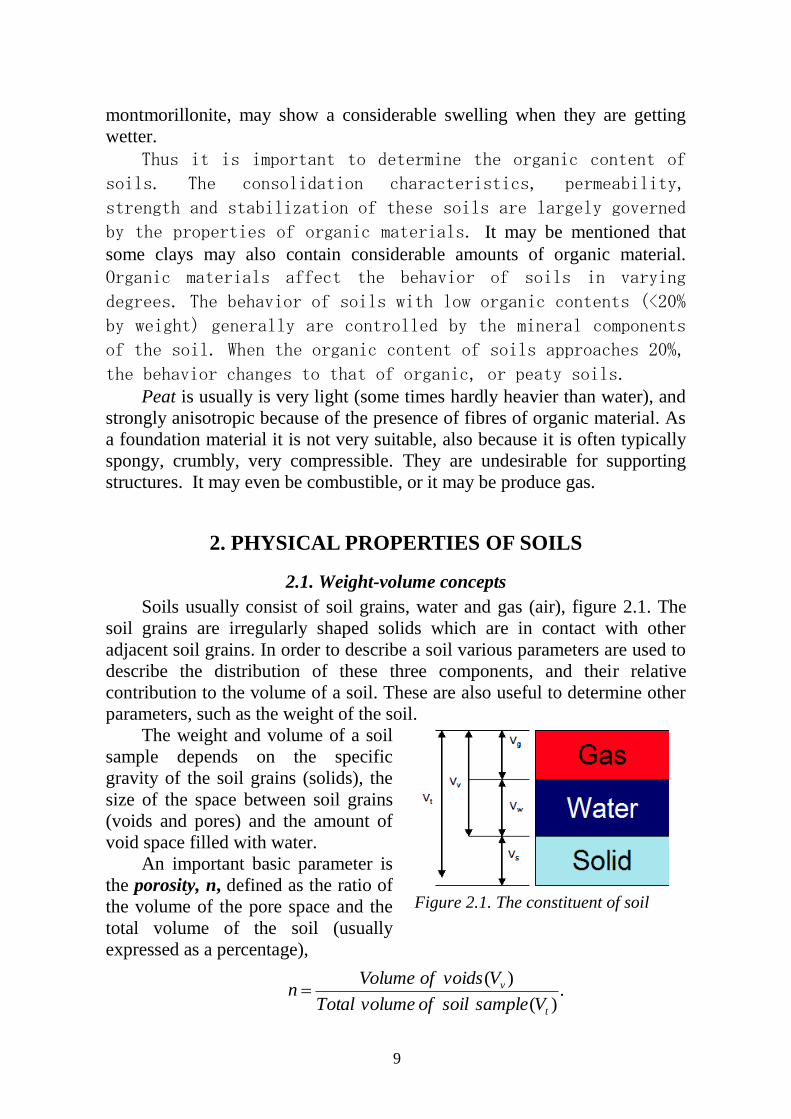
Soils usually consist of soil grains, water and gas (air), figure 2.1. The

soil grains are irregularly shaped solids which are in contact with other

adjacent soil grains. In order to describe a soil various parameters are used to

describe the distribution of these three components, and their relative

contribution to the volume of a soil. These are also useful to determine other

parameters, such as the weight of the soil.

The weight and volume of a soil

sample depends on the specific

gravity of the soil grains (solids), the

size of the space between soil grains

(voids and pores) and the amount of

void space filled with water.

An important basic parameter is

the porosity, n, defined as the ratio of

the volume of the pore space and the

total volume of the soil (usually

expressed as a percentage),

.

)(

)(

t

v

VsamplesoilofvolumeTotal

VvoidsofVolumen

Figure 2.1. The constituent of soil

10

For most soils the porosity is a number between 0,30 and 0,45 (or, as it

is usually expressed as a percentage, between 30 % and 45 %). When the

porosity is small the soil is called densely packed, when the porosity is large

it is loosely packed.

The amount of pores can also be expressed in the void ratio e, defined as

the ratio of the volume of the pores to the volume of the solids,

In many countries this quantity is preferred to the porosity, because it

expresses the pore volume with respect to a fixed volume (the volume of the

solids). Because the total volume of the soil is the sum of the volume of the

pores and the volume of the solids,

Vt = Vv + Vs.

This value can be determined directly by weighing a volume of dry soil.

In order to dry the soil a sample may be placed in an oven. The temperature

in such an oven is usually close to 100 degrees, so that the water will

evaporate quickly. At a much higher temperature there would be a risk that

organic parts of the soil would be burned.

The porosity and the void ratio can easily be related,

e = n/(1 –n);

n=e/(1+e ).

This is a common method to determine the porosity in a laboratory.

Unfortunately, this procedure is not very accurate for soils that are

almost completely saturated, because a small error in the measurements may

cause that one obtains, for example, S = 0,97 rather than the true value S =

0,99. In itself this is rather accurate, but the error in the air volume is then

300 %. In some cases, this may lead to large errors, for instance when the

compressibility of the water-air-mixture in the pores must be determined.

2.2. Water content

Water content, w, is defined as the ratio, expressed as a percentage, of

the weight of water in a given soil mass to the weight of solid particles. The

water content is especially useful parameter, particularly for clays.

.)(

)(

s

v

VsolidsofVolume

VvoidsofVolumee

11

Determination of the moisture content of soils is the most commonly used

laboratory procedure. Purpose is to determine the amount of water present in

a quantity of soil in terms of its dry weight and to provide general

correlations with strength, settlement, workability and other properties. The

moisture content of soils, when combined with data obtained from other tests,

produces significant information about the characteristics of the soil. For

example, when the in situ moisture content of a sample retrieved from below

the phreatic surface approaches its liquid limit, it is an indication that the soil

in its natural state is susceptible to larger consolidation settlement.

By definition the water content w is the ratio of the weight (or mass) of

the water and the solids:

The method of moisture content determination in laboratory conditions

specifies the amount of water contained in soil. It is done by drying the soil

sample at a temperature of about 105±5 o C to a constant weight (evaporate

free water); this is usually achieved in 12 to 24 hours.

Apparatus: thermostatically controlled oven maintained at a temperature

of 105± 5оC; weighing balance, with accuracy of 0.04% of the mass of the

soil taken; airtight container made of non-corrodible material with lid; tongs.

Procedure

1. Clean the container, dry it and weight it with lid (M1).

2. Take the required quantity of the wet specimen in the container and

clean it with lid. Take the mass (M2). The soil specimen should be

representative of the soil mass. The quantity of the specimen taken would

depend upon the gradation and the maximum size particles.

3. Place the container, with its lid removed, in the oven till its mass

becomes constant (Normally for 24 hours).

4. When the soil has dried, remove the container from the oven, using

tongs.

5. Find the mass (M3) of the container with lid and dry soil sample.

The water content (w) of a soil sample is equal to the mass of water

divided by the mass of solids:

w = [(M2 – M3) / (M3 – M1)] x100;

where M1 – Mass of empty container, with lid; M2 – Mass of the container

with wet soil & lid; M3 – Mass of the container with dry soil & lid.

For organic soils, a reduced drying temperature of approximately 40-60 oC is recommended. The wet sample is weighed, and then oven-dried to a

%.100)(

)(

s

w

MsolidssoilofMass

MwaterofMassw

12

constant weight at. The weight after drying is the weight of solids. The

change in weight, which has occurred during drying, is equivalent to the

weight of water.

Serious errors may be introduced if the soil contains other components,

such as petroleum products or easily ignitable solids. When the soils contain

fibrous organic matter, absorbed water may be present in the organic fibers as

well as in the soil voids. The test procedure does not differentiate between

pore water and absorbed water in organic fibers (although the procedure does

suggest evaluating organic soils at a lower temperature of 60 oC to reduce

decomposition of highly organic soils). Thus the moisture content measured

will be the total moisture lost rather than free moisture lost (from void

spaces).

Degree of saturation. Degree of saturation, S, is the ratio (expressed as a

percentage) of the volume of water in a given soil mass to the total volume of

voids. The pores of a soil may contain water and air. To describe the ratio of

these two the degree of saturation S is introduced as

Here Vw is the volume of the water, and Vv is the total volume of the pore

space. The volume of air (or any other gas) per unit pore space then is 1. For

a completely saturated soil (S = 1) and assuming that p/w = 2.65, it follows

that void ratio e is about 2.65 times the water content.

2.3. Density

The term density refers to mass per unit volume. The density of a mass

of soil is of interest to the engineer for a variety of reasons including the

design of earthworks and foundations and in slope stability analysis.

Dry unit weight, or dry density, is the weight of ovendried soil solids

per unit of total volume of soil mass. Dry density is – the density of the soil

in dry state:

Wet density, is the weight (solids plus water) per unit of total volume of

soil mass, irrespective of the degree of saturation. Volume density of soil

with natural moisture is expressed as a ratio of the weight and total volume of

a sample with natural moisture

.

)(

)(

t

ws

VsamplesoilofvolumeTotal

MMsamplesoilofMass

%.100)(

)(

v

w

VvoidsofvolumeTotal

VwatercontainsvoidsofvolumeTotalS

.)(

)(

t

sd

VsamplesoilofvolumeTotal

MsolidssoilofMass

13

Ms+Mw – mass of soil solids and water (0%<S<100%, unsaturated), Vt –

volume of a sample with natural moisture, units: kg/m3

Saturated density (S=100%)

The test consists in determining the moisture content of a volume unit of

soil. It is determined as a quotient of soil weight and its volume. In laboratory

conditions, volume density is determined using a sampling ring, by direct

calculation of volume (for samples of regular geometric shape) or by means

of underwater weighing. This sets the limitations concerning the applicability

of laboratory methods, which include the following soil types:

fine-grained cohesive soils of soft to stiff consistency without sand

admixture – sampling ring or cylinder method, underwater weighing method;

fine-grained cohesive soils of solid consistency – underwater weighing

method;

fine-grained cohesive soils with sand admixture up to 2 mm, single

grains or chips up to 4 mm – sampling cylinder method.

For the description of the density and the volumetric weight of a soil, the

densities of the various components are needed. For water the density is

denoted by w, and its value is about 1000 kg/m3. Small deviations from this

value may occur due to temperature differences or variations in salt content.

In soil mechanics these are often of minor importance, and it is often

considered accurate enough to assume that w = 1000 kg/m3. For the analysis

of soil mechanics problems the density of air can usually be disregarded.

Particle density or specific gravity of the soil grains is a measure of the

actual particles which make up the soil mass and is defined as the ratio of the

mass of the particles to the mass of the water they displace. A knowledge of

the particle density is essential in relation to other soil tests. A value of

specific gravity is necessary to compute the void ratio of a soil and porosity,

it is used in the hydrometer analysis, and it is useful to predict the unit weight

of a soil and is particularly important when compaction and consolidation

properties are being investigated.

The density of the solid particles depends upon the actual composition of

the solid material. Specific gravity of the soil grains typically varies between

2600 and 2800 kg/m3. In many cases, especially for quartz sands, its value is

about s = 2650 kg/m3, for clay – s = 2750 kg/m

3. Occasionally, the specific

gravity may be useful in soil mineral classifications; e.g., iron minerals have

.)(

)(

t

wssat

VsamplesoilofvolumeTotal

MMwatersolidssoilofMass

14

a larger value of specific gravity than silica.

The specific gravity is determined as the ratio of the weight of a given

volume of soil solids at a given temperature to the weight of an equal volume

of distilled water at that temperature, both weights being taken in air:

G = ρs/ρw.

Apparatus: 50 ml density bottle

with stopper (figure 2.2); оven;

constant temperature water bath

(27оC); vacuum desiccator; weighing

balance of accuracy 0,001 g; spatula.

Procedure

1. Clean the bottle with distilled water, dry it in oven, cool in desiccator

and weigh it with stopper.

2. Keep about 10-15 g of this soil in the bottle. Disturbed soil sample is

enough for this test. Take pulverized soil passed through 2 mm sieve.

3. Cover the soil with air free distilled water from the glass wash bottle

and leave for a period of 2 to 3 hours for soaking. Add water to fill the bottle

to about half.

4. Entrapped air can be removed by heating the density bottle on a water

bath or a sand bath.

5. Keep the bottle without stopper in vacuum desiccator for about 1 to 2

hours until there is no further loss of air.

6. Gently stir the soil in the density bottle by a clean glass rod, wash off

carefully adhering particles from the rod with some drops of distilled water

and see that no more soil particles are lost.

7. Repeat the process till no more air bubbles are observed in the soil

water mixture.

8. Observe the temperature of the constant in the bottle and record.

9. Insert the stopper in the density bottle, wipe and weigh.

10. Now make the bottle empty, clean thoroughly till the density bottle

with distilled water at the same temperature. Insert the stopper in the bottle,

wipe dry from the out side and weigh.

11. Take at least two such observations for the same soil.

Some qualifying words like true, absolute, apparent, bulk or mass, etc.

are sometimes added to "specific gravity". These qualifying words modify

the sense of specific gravity as to whether it refers to soil grains or to soil

mass. The soil grains have permeable and impermeable voids inside them. If

all the internal voids of soil grains are excluded for determining the true

volume of grains, the specific gravity obtained is called absolute or true

Figure 2.2. Density Bottles

15

specific gravity. Complete de-airing of the soil-water mix during the test is

imperative while determining the true or absolute value of specific gravity.

The unit weight is frequently used than the density is (e.g. in calculating

the overburden pressure).

,,Volume

gMass

Volume

WeightweightUnit

.8.9,

,sec8.9

3

2

mkNWater

mg

The measurement of unit weight for undisturbed soil samples in the

laboratory is simply determined by weighing a portion of a soil sample and

dividing by its volume. This is convenient with thin-walled tube (Shelby)

samples, as well as piston, Sherbrooke, Laval, and others samplers, as well.

The water content should be obtained at the same time to allow conversion

from total to dry unit weights, as needed.

Where undisturbed samples are not available, the unit weight is

evaluated from weight-volume relations between the water content and/or

void ratio, as well as the assumed or measured degree of saturation.

2.4. Standard compaction test

Purpose of standard compaction test is to determine the maximum dry

density attainable under specified nominal compaction energy for a given soil

and the (optimum) moisture content corresponding to this density. In the

construction of highway embankments, earth dams, retaining walls, structure

foundations and many other facilities, loose soils must be compacted to

increase their densities. Compaction increases the strength and stiffness

characteristics of soils. Compaction also decreases the amount of undesirable

settlement of structures and increases the stability of slopes and

embankments. Where a variety of soils are to be used for construction, a

moisture-density relationship for each major type of soil present at the site

should be established.

The void ratio is also used in combination with the relative density. This

quantity is defined as

DR = 100 (emax – e)/(emax – emin) .

Here emax is the maximum possible void ratio, and emin the minimum

possible value.

16

These values may be determined in the laboratory. The densest packing

of the soil can be obtained by strong vibration of a sample, which then gives

emin. The loosest packing can be achieved by carefully pouring the soil into a

container, or by letting the material subside under water, avoiding all

disturbances, which gives emax.

The accuracy of the determination of these two values is not very large.

After some more vibration the sample may become even denser, and the

slightest disturbance may influence a loose packing. It follows from equation

that the relative density varies between 0 and 1. A small value, say DR < 0.5,

means that the soil can easily be densified. Such a densification can occur in

the field rather unexpectedly, for instance in case of a sudden shock (an

earthquake), with dire consequences.

Compaction is the process of densification of soil by reducing air voids.

The degree of compaction of a given soil is measured in terms of its dry

density. The dry density is maximum at the optimum water content. A curve

is drawn between the water content and dry density to obtain the maximum

dry density and optimum water content.

Dry density = (M / V)/(1+w),

where M = total mass of soil, V = volume of soil; w = water content

Apparatus: cylindrical metal compaction mould (capacity : 1000 cc with

dia 100 mm + 0.1; 2250 cc with dia 150 mm + 0.1; internal diameter : 100

mm + 0.1; 150 mm + 0.1; internal effective height of mould : 127.3 + 0.1 mm;

collar : 60 mm high; detachable base plate; hammer mass: for light

compaction = 2.5 kg; heavy compaction = 4.6 kg; dia : 50 mm; sieve; oven :

thermostatically controlled to maintain a temperature of 105оC; weighing

balance : sensitivity – 1 g for capacity 10 kg; 0.01g for capacity 200 g; steel

straight edge of about 300 mm in length with one edge leveled; gradation jar;

large mixing pan; spatula.

Procedure

1. Preparation of sample. A representative portion of air dried soil

sample (in case of oven drying temp. < 60 оC) break the clods, remove the

organic matter like free roots, piece of bark etc.

2. Take about 6 kg – (for soil is not susceptible to crushing during

compaction) 15 kg – (for soil is susceptible to crushing during compaction).

Sieve above material through 19 mm sieve and 4.75 mm sieve and % passing

4.75 mm sieve. Do not use the soil retained on 20 mm sieve. Determine the

ratio of fraction retained and that passing 4.75 mm sieve. If % passing

retained on 4.75 mm sieve is greater than 20 mm sieve, use the larger mould

17

of 150 mm diameter. Mix the soil sample retained on 4.75 mm sieve and that

passing 4.75 mm sieve in the proportion determined.

3. Thoroughly mix water in sandy and gravely soil : 3 to 5 %; cohesive

soil : 12 to 16 % approx.

4. Store the soil sample in

a sealed container for minimum

period of 16 hours.

5. Clean and dry the mould

and base plate. And apply a thin

layer of grease on inside the

mould.

6. Weigh the mould to the

nearest 1 gram. Attach the collar

to the mould and place on a solid

base.

7. Compact the moist soil

in to the mould in five layers of

approximately equal mass, layer

being given 25 blows from 4.54

kg hammer dropped from the

height of 457 mm above the soil

(figure 2.3). The blows should

be distributed uniformly over the

surface of each layer.

8. Remove the collar and

trim off the excess soil projecting above the mould by using straight edge.

Take the weight of mould with compacted soil in it.

9. Remove the 100 g compacted soil specimen for the water content

determination.

10. Add water in increment of 1 to 2 % for sandy and gravely soils and 2

to 4 % for cohesive soils.

11. Above procedure will be repeated for each increment of water added.

The total number of determination shall be at least four. Hamming

should be done continuously taking of height of 457 mm free fall accurately.

The amount of soil taken for compaction should be in such a way that after

compacting the last layer, the soil surface is not more than 5 mm above the

top rim of the mould. Weighing should be done accurately.

Procedure of Compaction tests are performed using disturbed, prepared

soils with or without additives. Normally, soil passing the sieve is mixed with

water to form samples at various moisture contents ranging from the dry state

to wet state. The order of soil preparation is showed on figure 2.4. Dry

Figure 2.3. Compaction - Lab Equipment

18

density is determined based on the moisture content and the unit weight of

compacted soil.

The density of soils is measured as the unit dry weight, d, (weight of

dry soil divided by the bulk volume of the soil). It is a measure of the amount

of solid materials present in a unit volume. The higher the amount of solid

materials, the stronger and more stable the soil will be.

A curve of dry density versus moisture content is plotted in figure 2.5

and the maximum ordinate on this curve is referred to as the maximum dry

density. The water content at

which this dry density occurs is

termed as the optimum

moisture content. To provide a

“relative” measure of

compaction, the concept of

relative compaction is used.

Relative compaction is the

ratio (expressed as a percentage)

of the density of compacted or

natural in-situ soils to the

maximum density obtainable in

a compaction test. Often it is

necessary to specify the

achieving of a certain level of

2

Figure 2.4. Procedure of soil preparation for compaction tests

Figure 2.5. Representative moisture-density

relationship from a standard compaction test.

19

relative compaction (e.g. 95%) in the construction or preparation of

foundations, embankments, pavement sub-bases and bases, and for deep-

seated deposits such as loose sands. The design and selection of a placement

method to improve the strength, dynamic resistance and consolidation

characteristics of deposits depend heavily on relative compaction

measurements.

It is also convenient to plot the zero air voids (ZAV) curve on the

moisture-density graph, corresponding to 100 percent saturation (see figure

2.5). The measured compaction curve response should not fall on or above

this ZAV line. The maximum dry unit weight (“density”) found as the peak

value often corresponds to saturation levels of between 70 to 85 percent.

3. CLASSIFICATION TESTS OF SOILS

3.1. Grain-Size Analysis

Soil index properties are used extensively by engineers to discriminate

between the different kinds of soil within a broad category, e.g. clay will

exhibit a wide range of engineering properties depending upon its

composition. Classification tests to determine index properties will provide

the engineer with valuable information when the results are compared against

empirical data relative to the index properties determined. The gradation tests

are performed to determine the particle size distribution of the soil which

could be used for soil classification.

Grain-size analysis is a process in which the proportion of material of

each grain size present in a given soil (grain-size distribution) is determined.

The tests consist of two types: sieve analysis for coarse-grained soils (sands,

gravels), hydrometer analysis for fine-grained soils (clays, silts). Materials

containing both types of soils are tested by both methods and the results are

merged to create one particle size distribution result. These tests shall be

performed on samples that were obtained for verification of the field

classification of the major soil types encountered during the investigation.

The number of tests shall be limited to reasonably establish the stratification

without duplication, unless approved otherwise. A minor soil type, if not

critical, may be given a visual classification, instead of performing

classification tests for reference.

Sieve analyze. The usual procedure is to use a system of sieves having

different mesh sizes, stacked on top of each other, with the coarsest mesh on

top and the finest mesh at the bottom.

Apparatus: set of fine sieves; set of coarse sieves; weighing balance,

with accuracy of 0.1% of the mass of sample; оven; mechanical shaker;

20

mortar, with rubber pestle; brushes; trays.

Figure 3.1 shows a selection of sieves and soil particle sizes. Sieves

larger than the #4 sieve are designated by the size of the openings in the sieve.

Smaller sieves are numbered according to the number of openings per inch.

Special standardized sets of sieves are available, as well as convenient

shaking machines (Figure 3.2). Hand sieving of a large number of samples

can often be tedious and sometimes lead to inaccuracy of results. Shaker

machines are ideal for laboratory or on site use. The machines provide a wide

choice of options for the busy laboratory. Shakers are robust, compact and

sufficiently lightweight to be portable. The digital display incorporated in the

unit makes the setting of the microprocessor controlled functions very

straightforward. The unique action of the sieve shaker imparts a circular

motion to the material being sieved so that it makes a slow progression over

the surface of the sieve. At the same time, a rapid vertical movement agitates

the sample which assists in clearing the apertures. A variable time switch,

with a range of 10 to 60 minutes, is incorporated to set the duration of test.

The shaker stops automatically at the end of set duration. The Octagon

(figure 3.2) is powered by an electromagnetic drive that has no rotating parts

to wear making it maintenance free and extremely quiet in operation.

21

The vibratory action produced by the power unit moves the sample over

the sieve in a unique way producing faster more efficient sieving, while the

rapid vertical movements also help keep the apertures from blinding.

Procedures

1. Soil sample, as received from the field shall be dried in air or in sun.

In wet weather the drying apparatus may be used in which case the

temperature of the sample should not exceed 60 оC.

2. The clod may be broken with wooden mallet to hasten drying the

organic matter, like tree root and pieces of bark should be removed from the

sample.

3. The big clods may be broken with the help of wooden mallet.

4. Care should be taken not to break up the individual soil particles.

5. A representative soil sample of required quantity is taken and dried in

oven at 105 -120 оC.

6. The dried sample is taken in tray and soaked with water and mixed 2

g of sodium hexametaphosphate of 2 g or sodium hydroxide of 1 g and

sodium carbonate of 1 g per liter of water added as dispersive agent. The

soaking of soil continued for 10 -12 hours.

7. Sample is washed through 4.75 mm sieve with water till substantially

clean water comes out. Retained sample on sieve shall be oven dried for 24

hours. This dried sample is sieved through 20 mm, 10 mm set of sieves.

8. The portion of the passing sieve shall be oven dried for 24 hours.

This oven dried material is riffled and is taken of about 200 g.

9. This sample of about 200 g is washed on 75 micron sieve with half

litre distilled water till substantially clear water comes out.

10. The material retained on 75 μ IS sieve is

collected and dried in oven at 105 - 120 оC for 24

hours. The dried soil sample is sieved through 2 mm,

600 μ, 425 μ, 212 μ sieves. Soil retained on each

sieve is weighed.

11. If the soil passing 75 μ is 10% or more,

hydrometer method is used to analysis soil particle

size.

After shaking the assembly of sieves, by hand

or by a shaking machine, each sieve will contain the

particles larger than its mesh size, and smaller than

the mesh size of all the sieves above it. In this way

the grain size diagram can be determined. The

amount retained on each sieve is collected dried and

weighed to determine the percentage of material

Figure 3.1 Soil particle sizes and selection of sieves.

Figure 3.2. Sieve shaker

22

passing that sieve size.

Obtaining a representative specimen is an important aspect of this test.

When samples are dried for testing or “washing,” it may be necessary to

break up the soil clods. Care should be made to avoid crushing of soft

carbonate or sand particles. If the soil contains a substantial amount of

fibrous organic materials, these may tend to plug the sieve openings during

washing. The material settling over the sieve during washing should be

constantly stirred to avoid plugging.

Openings of fine mesh or fabric are easily distorted as a result of normal

handling and use. They should be replaced often. A simple way to determine

whether sieves should be replaced is the periodic examination of the stretch

of the sieve fabric on its frame. The fabric should remain taut; if it sags, it has

been distorted and should be replaced. A common cause of serious errors is

the use of “dirty” sieves. Some soil particles, because of their shape, size or

adhesion characteristics, have a tendency to be lodged in the sieve openings.

Hydrometer Analysis. This method determines particle size distribution

(percentage) of particle sizes, and identify the silt, clay, and colloids

percentages in the soil. This is because the soil behavior for a cohesive soil

depends principally on the type and percent of clay minerals, the geologic

history of the deposit, and its water content rather than on the distribution of

particle sizes. For particles smaller than about 0.05 mm according to USCS

(0.075 mm according to British standards) the grain size can not be

determined by sieving, because the size of the holes in the mesh would

become unrealistically small, and also because during shaking the small

particles might by up in the air, as dust.

Soil passing the sieve is mixed with dispersant and distilled water and

placed in a special graduated cylinder in a state of liquid suspension (Fig. 3.3).

Mechanical End-over-End Shaker (figure 3.3. b) fitted with friction

safety device, capable of rotating two Jars at approximately 50 rpm.

Mechanical analysis stirrer (figure 3.3. c) is used for dispersing soil samples

in water for hydrometer analysis. The stirrer is supplied complete with

mixing paddle and dispersion cup. The specific gravity of the mixture is

periodically measured using a calibrated hydrometer (Figure 3.3. d) to

determine the rate of settlement of soil particles.

Procedures

1. Particles passed through 75 μ sieve along with water is collected and

put into a 1000 ml jar for hydrometer analysis. More water if required is

added to make the soil water suspension just 1000 ml. The suspension in the

jar is vigorously shaken horizontally by keeping the jar in between the palms

of two hands. The jar is put on the table.

23

2. A graduated hydrometer is carefully inserted in to the suspension with

minimum disturbance.

3. At different time intervals, the density of the suspension at the c.g. of

the hydrometer is noted by seeing the depth of sinking of the stem. The

temperature of suspension is noted for each recording of hydrometer reading.

4. Hydrometer reading is taken at a time of 0.5, 1.0, 2.0, 4.0, 15.0, 45.0,

90.0, 180.0 minutes, 6 hrs, 24 / 48 hours.

5. By using the nomogram the diameter of the particles at different

hydrometer reading is found out.

The amount of particles of a particular size can then be determined much

better by measuring the velocity of deposition in a glass of water. This

method is based upon a formula derived by Stokes for settlement of idealized

spherical particles. This formula expresses that the force on a small sphere,

sinking in a viscous liquid, depends upon the viscosity of the liquid, the size

of the sphere and the velocity. It should be noted that Stokes Law does not

apply to particles < 0.0002mm.

Because the force acting upon the particle is determined by the weight of

а) b)

c) d) Figure 3.3. Apparatus: a) hydrometer sedimentation cylinders b) end-over-end

Shaker, c) stirrer, d) soil hydrometers

24

the particle under water, the velocity of sinking of a particle in a liquid can be

derived. The formula is

18

)( 2Dv

fp

(3.1)

where p - is the volumetric weight of the particle, f - is the volumetric

weight of the liquid, D - is the grain size, µ - is the dynamic viscosity of the

liquid.

Because for very small particles the velocity may be very small, the test

may take rather long. The test does not require the weighing accuracy

necessary for pipette sedimentation and is suitable for use in site laboratories.

Replicable results can be obtained when soils are largely composed of

common mineral ingredients. Results can be distorted and erroneous when

the composition of the soil is not taken into account to make corrections for

the specific gravity of the specimen. Particle size of highly organic soils

cannot be determined by the use of this method.

The Pipette Method produces similar results to the hydrometer method,

but is considered to be more precise. It requires delicate apparatus and greater

accuracy in weighing. In the pipette test samples of a suspension are taken

from a fixed elevation in a measuring cylinder at times, t, and the percentage

of various grain sizes determined.

Andreasen Pipette Stand (figure 3.4.) with

moving carriage assembly which can be

operated with no vibration transmitted to

the pipette whilst the pipette is being

inserted and withdrawn from the liquid

suspension. The stand is fitted with a

holder for securing the pipette and is

supplied with a stand for the sedimentation

cylinder.

Specially designed for the

sedimentation testing of soils and other

fine grained material, the bath is supplied

with a false bottom to assist in circulation

of the bath liquid. Adequate clearance is

provided when the tank is used with a

Pipette sedimentation stand.

Figure 3.4. Pipette Stand

25

Results of grain tests

are sometimes needed to

complete classification of

soils. Figure 3.5 shows

several grain size

distributions obtained from

sieving and hydrometer

methods. Shown (right to

left) are sieve and example

soil particle sizes

including (right to left):

medium gravel, fine gravel,

medium-coarse sand, silt,

and dry clay (kaolin).

The size of the particles in a certain soil can be represented graphically

in a grain size diagram (figure 3.6). Such a diagram indicates the percentage

of the amount of particles smaller than a certain diameter, measured as a

percentage of the weight. The results are plotted on a semi log graph with

particle size as abscissa (log scale) and the percentage smaller than the

specified diameter as ordinate. A steep slope of the curve in the diagram

indicates a uniform soil, a shallow slope of the diagram indicates that the soil

contains particles of strongly different grain sizes.

The resulting gradations can provide data for determining several

parameters, such as effective diameter (D10) and coefficient of uniformity

Figure 3.6. Grain-size diagram

Figure 3.5. Sieves for mechanical analysis for grain

size distributions.

26

(Cu). The grain size distribution can be characterized by the quantities D60

and D10. These indicate that 60 %, respectively 10 % of the particles

(expressed as weights) is smaller than that diameter. The ratio of these two

numbers is denoted as the uniformity coefficient Cu,

Cu = D60/D10 .

In a poorly graded soil the particles all have about the same size. The

uniformity coefficient is than only slightly larger than 1, say Cu = 2.

3.2. Consistency (Atterberg) Limits

The Atterberg limits provide general indices of moisture content relative

to the consistency and behavior of cohesive soils. With high moisture content,

silty clay becomes slurry to liquid. Liquid consistency corresponds to the

case when soil shows practically no resistance to shear strain. After

significant reduction of its moisture content, soil obtains characteristics of a

brittle material, and when exposed to strain it fails. This state is called stiff

consistency.

Purpose the Atterberg limits tests is to describe the consistency and

plasticity of fine-grained soils with varying degrees of moisture. For the

portion of the soil passing the № 40 sieve, the moisture content is varied to

identify three stages of soil behavior in terms of consistency. These stages are

known as the liquid limit (LL), plastic limit (PL) and shrinkage limit (SL) of

soils. In total, individual consistencies and limits may be graphically

displayed as follows phases on figure 3.7.

Figure 3.7. The Atterberg limits and phases of soils

27

The liquid limit. The moisture content at which soil already shows some

shear strength is considered to be the boundary between liquid and plastic

consistency. It is called the liquid limit (LL), units: %.

Procedure of the definition of the liquid limit test by manual Casagrande

cup device. As this limit is not absolute, it has been defined as the value

determined in a certain test, due to Casagrande. The test procedure has

remained, in principle, the same since 1932, when Casagrande proposed to

define the various limits by relating the moisture content characteristics of

soil under certain conditions.

The liquid limit is determined in a standardized Casagrande dish. The

apparatus required is simple yet effective. The soil in the dish is divided by a

cutting knife into 2 parts, and the whole dish falls on a pad from a height of 1

cm. In the test a hollow container with a soil sample may be raised and

dropped by rotating an axis (figure 3.8). The liquid limit is the value of the

water content for which a standard V-shaped groove cut in the soil, will just

close after 25 drops. If both parts along the cut are reconnected at a length of

12.5 mm after 25 blows, the soil's moisture content is at its liquid

limit. When the groove closes after less than 25 drops, the soil is too wet, and

some water must be allowed to evaporate. By waiting for some time, and

perhaps mixing the clay some more, the water content will have decreased,

and the test may be repeated, until the groove is closed after precisely 25

drops. Then the water content must immediately be determined, before any

more water evaporates, of course.

Figure 3.8. The definition of the liquid limit by manual Casagrande cup device

28

Procedure 1. Air dry the soil sample (in case drying) and break the clods. Remove

the organic matter like tree roots, pieces of bark etc.

2. About 100 g of the specimen passing 425 micron IS sieve is mixed

thoroughly with distilled water in the evaporating dish and left for 24 hours

for soaking.

3. A portion of the paste is placed in the cup of the Liquid limit device.

4. Level the mix so as to have a maximum depth of 1 cm.

5. Draw the grooving tool through the sample along the symmetrical

axis of the cup, holding the tool perpendicular to the cup.

6. For normal fine grained soil: the Casagrande tool is used which cuts a

groove of width 2 mm at the bottom, 11 mm at the top and 8 mm deep.

7. For sandy soil : The tool is used which cuts a groove of width 2 mm

at bottom, 13.6 mm at top and 10 mm deep.

8. After the soil pat has been cut by proper grooving tool, the handle is

rotated at the rate of about 2 revolutions per second and the nos. of blows

counted till the two parts of the soil sample come into contact for about 10

mm length.

9. Take about 10 g of soil near the closed groove & find water content.

10. The soil of the cup is transferred to the dish containing the soil paste

and mixed thoroughly after adding a little more water. Repeat the test.

11. By altering the water content of the soil and repeating the foregoing

operations, obtain at least 5 readings in the range of 15 - 35 blows. Don‟t mix

dry soil to change its consistency.

12. Liquid limit is determined by plotting a „flow curve‟ on semi-log

graph between nos. of blows on logarithmic scale and water content on

arithmetical scale.

13. Generally these points lie in a straight line.

14. Water content corresponding to 25 blows is the value of Liquid limit.

An alternate procedure for Casagrande‟s test in Europe and Canada uses

a fall cone device to obtain better repeatability (figure 3.9). In this test a steel

cone, of 60 grams weight, and having a point angle of 60o, is placed upon a

clay sample, with the point just at the surface of the clay. The cone is then

dropped and its penetration depth is measured. The liquid limit has been

defined as the water content corresponding to a penetration of exactly 10 mm.

29

Procedure

1. The 4 numbered cans were weighed.

2. The container of the cone penetrometer device was

filled with soil specimen on three times, and were stroke on

the bench to prevent air voids from taking place in the

container, and it was stuck flush.

3. The container containing the specimen was placed under

the cone of the penetrometer, and the cone is then released

for 5 seconds, and the reading of the penetration was taken.

4. Small portion of the tested soil was taken into one of

the identified cans and its weight was recorded.

5. The four cans were then removed to the oven for 24

hours, and then their weights were recorded.

Again the liquid limit can be determined by doing the test at various

water contents. It has also been observed, however, that the penetration depth,

when plotted on a scale, is an approximately linear function of the water

content (figure 3.10). This means that the liquid limit may be determined

from a single test, which is

much faster, although less

accurate.

Procedure of the

definition of the plastic limit.

The transitory moisture

content between plastic and

stiff consistency is called the

plasticity limit (PL). The

Figure 3.9. Fall Cone

Figure 3.10. Liquid Limit determined by doing

the test at various water contents

30

plasticity limit is determined by saturating soil with water and by making

rolls of it with a diameter of 3 mm (figure 3.11) on an absorbent pad. If the

rolls start to crumble into 1 cm lengths, the soil's moisture content is at its

plasticity limit.

Apparatus: porcelain evaporating dish about 120 mm diameter; spatula;

container to determine moisture content; balance with 0.01 g accuracy; oven;

ground glass plate 20 x 15 cm for rolling.

Procedure

1. Take out 30 g of air dried soil from a thoroughly mixed sample of the

soil passing sieve, mix the soil with distilled water in a evaporating dish and

leave the soil mass for naturing. This period may be up to 24 hours.

2. Take about 8 g of the soil and roll it with fingers on a glass plate. The

rate of rolling shall be between 80 to 90 strokes per minutes to form a 3 mm

diameter.

3. If the diameter of the threads becomes less than 3 mm without cracks,

it shows that water content is more than its plastic limit. Kneed the soil to

reduce the water content and roll it again to thread.

4. Repeat the process of alternate rolling and kneading until the thread

crumbles.

5. Collect the pieces of crumbled soil thread in a moisture content

container.

6. Repeat the process at least twice more with fresh samples of plastic

soil each time.

The definition of the plastic limit very wet clay can be rolled into very

thin threads, but dry clay will break when rolling thick threads. The (arbitrary)

limit of 3 mm is supposed to indicate the plastic limit. In the laboratory the

Figure 3.11. The definition of the plastic limit

31

test is performed by starting with a rather wet clay sample, from which it is

simple to roll threads of 3 mm. By continuous rolling the clay will gradually

become drier, until the threads start to break by evaporation of the water or

with help devise (figure 3.12).

Depending on their liquid limit, soils may be further specified as soils

showing the following plasticity (figure 3.13): L – low LL below 35 %, I –

medium LL = 35 – 50 %, H – high LL = 50 – 70 %, V – very high LL = 70 –

90 %, E – extremely high LL exceeding 90 %.

In countries with very thick clay deposits (England, Japan, Scandinavia,

Russia) it is often useful to determine a profile of the plastic limit and the

liquid limit as a function of depth, see figure 3.14. In this diagram the natural

water content, as determined by taking samples and immediately determining

Figure 3.12. Warm-air dryer and Willе Geotechnik equipment for the plastic limit

definition.

Figure 3.13. Specification of soil by consistency limit

32

the water content, can also be indicated.

On the basis of these consistеncy limits, the

characteristics of cohesive soils are determined –

their plasticity index PI, consistency index IC,

liquidity index IL and colloidal clay activity index

A.

Plasticity is expressed by means of the

plasticity index, which is the range of moisture

content at which soils show plastic behavior. For

many applications it is especially important that

the range of the plastic state is large. This is

described by the plasticity index PI. The plasticity

index is a useful measure for the possibility to

process the clay. It is important for potteries, for

the construction of the clay core in a high dam, and

for the construction of a layer of low permeability

covering a deposit of polluted material. In all these

cases a high plasticity index indicates that the clay

can easily be used without too much fear of it

turning into a liquid or a solid.

Plasticity index is defined as the difference of

the liquid limit and the plastic limit,

PI = LL - PL .

where LL - moisture content at liquid limit, PL - moisture content at

plasticity limit, units: non-dimensional.

The plasticity index PI grows with the percentage of clay fraction.

The consistency index is the most common way of expressing the

consistency of cohesive soils. Consistency index - Ic

Ic =(LL-w)/(LL-PL)

where LL - moisture content at liquid limit, PL - moisture content at plasticity

limit, w - specific moisture content of soil at which its consistency is

determined, units: non-dimensional.Depending on its value, the following

states (consistencies) are distinguished:

consistency index IC consistency

greater than or equals 1 solid to hard

1.0 - 0.5 Stiff

0.5 - 0.05 Soft

smaller than 0.05 slurry - liquid

Figure 3.14. Profile of the

plastic and the liquid limit

as a function of depth

33

In foreign academic literature, the consistency of cohesive soils is also

expressed by means of the index of liquidity IL.

IL=(w-PL)/(LL-PL),

where LL - moisture content at liquid limit, PL - moisture content at

plasticity limit, w - specific moisture content of soil at which its consistency

is determined, units: non-dimensional.

The liquidity index is LI = (w-PL)/PI is an indicator of stress history; LI

#1 for normally consolidated (NC) soils and LI #0 for over-consolidated (OC)

soils.

The colloidal clay activity index A was defined by Skempton in 1953.

Colloidal clay activity index - IA

A=PI / % clay fraction (weight)

PI - plasticity index , units: non-dimensional.

By and large, these are approximate and empirical values. They were

originally developed for agronomic purposes. Their widespread use by

engineers has resulted in the development of a large number of rough

empirical relationships for characterizing soils.

Considering the abstract and manual nature of the test procedure,

Atterberg limits should only be performed by experienced technicians. Lack

of experience, and lack of care will introduce serious errors in the test results.

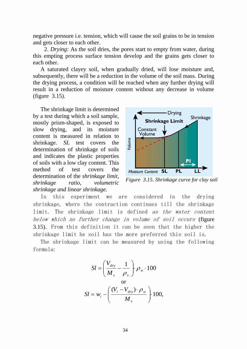
The shrinkage limit (SL). The transitory moisture content between its

stiff and solid consistency of the soil, in percent, at which the decrease in soil

volume ceases, is defined as the shrinkage limit, units: %. Volume changes

in soil can be a very dangerous problem in engineering structures; for

example if a soil used in a highway expands or contracts this will produce a

bumpy road. Volume changes occur over a period of time and depend on

both soil type and the change in water content, but most of the damage will

occur if differential water contents produce different amount of volume

change.

Shrinkage is soil contraction and is mainly a cause of soil suction, which

is the phenomenon that produces capillary rise of water in soil pores above

the water table. Two main sources of soil shrinkage are:

1. Capillary rise: At the top of the capillary column the pressure will be

A Classification Potential for swelling

< 0.75 Inactive Clays Low

0.75 – 1.25 Normal Clays Med

>1.25 Active Clays (e.g. montmorillonite) High

34

negative pressure i.e. tension, which will cause the soil grains to be in tension

and gets closer to each other.

2. Drying: As the soil dries, the pores start to empty from water, during

this empting process surface tension develop and the grains gets closer to

each other.

A saturated clayey soil, when gradually dried, will lose moisture and,

subsequently, there will be a reduction in the volume of the soil mass. During

the drying process, a condition will be reached when any further drying will

result in a reduction of moisture content without any decrease in volume

(figure 3.15).

The shrinkage limit is determined

by a test during which a soil sample,

mostly prism-shaped, is exposed to

slow drying, and its moisture

content is measured in relation to

shrinkage. SL test covers the

determination of shrinkage of soils

and indicates the plastic properties

of soils with a low clay content. This

method of test covers the

determination of the shrinkage limit,

shrinkage ratio, volumetric

shrinkage and linear shrinkage.

In this experiment we are considered in the drying

shrinkage, where the contraction continues till the shrinkage

limit. The shrinkage limit is defined as the water content below which no further change in volume of soil occurs (figure

3.15). From this definition it can be seen that the higher the shrinkage limit he soil has the more preferred this soil is.

The shrinkage limit can be measured by using the following

formula:

1001

w

ss

dry

M

VSl

or

,100)(

s

wdryi

iM

VVwSl

Figure 3.15. Shrinkage curve for clay soil

35

where: wi -Initial water content, Vdry - volume of final

volume (dry volume), Ms - mass of the dried sample. The test is simply held by placing the soil sample in the

shrinkage dish and stuck flush, and then dried gradually, so

that no cracking for the soil sample will occur, for 48 hours

where the first 24 hours will be air drying. Dry volumes in

equation can be approached by mercury method. Apparatus: shrinkage dish, having a flat bottom, 45 mm diameter and 15

mm height; two evaporating dishes about 120 mm diameters, with a pour out

and flat bottom; one small mercury dish, 60 mm diameter; two glass plates,

one plane and one with prongs, 75 x 75 x 3 mm size; glass cup, 50 mm

diameter and 25 mm height; sieve 425 micron; oven; desiccator; weighing

balance, accuracy 0.01 g; spatula; straight edge; mercury. Equipment for

definition of volumetric shrinkage limit are showed on figure 3.16.

36

Procedure

1. Take a sample of mass about 100 g from a thoroughly mixed soil

passing 425 micron sieve.

2. Take about 30 g of soil sample in a large evaporating dish. Mix it with

distilled water to make a creamy paste, which can be readily worked without

entrapping the air bubbles.

3. Take the shrinkage dish, clean it and determine its mass. The dish was

greased before starting the lab so that the soil won‟t stick on its walls.

4. Fill mercury in the shrinkage dish. Remove the excess mercury by

pressing the plain glass plate over the top of the shrinkage dish. The plate

should be flush with the top of the dish, and no air should be entrapped.

5. Transfer the mercury of the shrinkage dish to a mercury weighing dish

and determine the mass of the mercury to an accuracy of 0.01 g. The volume

of the shrinkage dish is equal to the mass of the mercury in grams divided by

the specific gravity of the mercury.

Figure 3.16. Apparatus for determining the volume of dry soil

37

6. Coat the inside of the shrinkage dish with a thin layer of silicon grease

or vaseline. Place the soil specimen in the center of the shrinkage dish, equal

to about one third volume of shrinkage dish. Tap the shrinkage dish on a firm,

cushioned surface and allow the paste to flow to the edges.

7. Add more soil paste, approximately equal to the first portion and tap

the shrinkage dish as before, until the soil is thoroughly compacted. Add

more soil and continue the tapping till the shrinkage dish is completely filled,

and excess soil paste projects out about it‟s edge. Strike out the top surface of

the paste with the straight edge. Wipe off all soil adhering to the out side of

the shrinkage dish. Determine the mass of the wet soil.

8. Dry the soil in the shrinkage dish in an air until the colour of pat turns

from dark to light. Then dry the pat in the oven at 105 to 110 оC to constant

mass.

9. Cool the dry pat in a desiccator. Remove the dry pat from the

desiccator after cooling and weigh the shrinkage dish with the dry pat to

determine the dry mass of the soil.

10. Place a glass cup in a large evaporating dish and fill it with mercury.

Remove the excess mercury by pressing the glass plate with prong firmly

over the top of the cup. Wipe of any mercury adhering to the outside of the

cup. Remove the glass cup full of mercury and place it in another evaporating

dish, taking care not to spill any mercury from the glass cup.

11. Take out the dry pat of soil from the shrinkage dish and immerse it

in the glass cup full of mercury. Take care not to entrap air under the pat.

Press the plate with the prongs on the top of cup firmly.

12. Collect the mercury displaced by the dry pat in the evaporating dish,

and transfer it to the mercury weighing dish. Determine the mass of mercury

to an accuracy of 0.01 g. The volume of the dry pat is equal to the mass of

mercury divided by the specific gravity of mercury.

13. Repeat the test at least 3 times.

The linear shrinkage is defined as the decrease in one dimension of a

soil mass, expressed as a percentage of the original dimension, when the

water content is reduced from a given value to the shrinkage limit. Standards

specifies a method for measuring the linear shrinkage, where standardized

mold takes the shape of half cylinder of 12.5 mm diameter and 140 mm

length (figure 3.17).

Using the following formula the Linear shrinkage is measured:

LS(%)=100%Ls/L

38

where L- initial length (the length of the mold), Ls- final length of the

specimen.

The mold is fill with soil sample and then dried in the same manner the

shrinkage sample was dried, and then the final length of the specimen was

measured. For purposes of accuracy several readings are taken for each

length and then the average for each reading is calculated and used in the

formula. The length of dried sample is measured by using a string and a ruler

as the specimen will be buckled and its length can‟t be measured by using a

ruler only.

Procedure

1. The standardized mold was filled with soil sample to the top and the

surface was leveled.

2. The mold containing the sample was then placed into the oven and

dried gradually to avoid cracking of the soil sample.

3. After 48 hours, the mould was removed from the oven and the length

of the mold was measured two times and the length of the specimen was

measured 3 times.

In the case of heavy clay soils, it is desirable to allow the wet soil to

stand for about 24 hours in an airtight container before performing the test to

allow the water to permeate throughout the soil mass. After curing, it is

necessary to re-mix before testing. Highly aggregated soil may require as

much as 40 minutes continuous mixing immediately before testing.

As operators gain experience, it will not be necessary to test the mixture

in the liquid limit machine as moisture content is not critical within a few per

cent. The curling of a specimen can generally be prevented by extremely

slow drying.

Alternatively, when excessive curling is expected, the specimens may be

air-dried for 24 hours and then weighted in three places in such a manner to

prevent undue curling but to allow moisture to evaporate.

It is possible to prepare a special scale calibrated for the length of the

mould to read off linear shrinkage direct. For a 250 mm mould, scale

Figure 3.17. Linear Shrinkage apparatus

39

subdivisions of 1.25 mm correspond to 0.5% increments of linear shrinkage.

For a 135 mm mould, scale subdivisions of 1.35 correspond to 1%

increments of linear shrinkage.

3.3. Classification of Soils

Classification helps in grouping soils according to properties, provides a

way of referring to soils universally, and makes selection of soils easy for a

certain application. The engineering classification of soils can be used as a

preliminary estimate of the potential engineering use of soils. Will the soils

be freely draining or impermeable, will they be highly compressible etc.

These factors are obviously important in choosing a suitable material for the

core material of an earth dam or for the foundation of a building. Some soils

are liable to collapse, others to liquefaction. Some clays containing high

montmorillonite contents are particularly susceptible to shrinkage and

swelling with seasonal changes in water content.

Various engineering classifications of soils have been adopted

throughout the world. There are US systems, French systems, Russian

systems, Australian systems, Brazilian systems, British systems, Canadian

systems, Dutch systems, German systems, Polar systems and others.

The global character of a classification according to grain size is well

illustrated by the characterization sometimes used in Germany, saying that

gravel particles are smaller than a chicken‟s egg and larger than the head of a

match, and that sand particles are smaller than a match head, but should be

visible to the naked eye.

Soils may be crudely classified also according to grain size, table 3.1, in

to fine grained (predominantly clay and silt size) or coarse grained (sand and

gravel sizes predominant ); or in shear strength terms: cohesive (eg. clays,

clay silt mixtures, organics) – (c-soils or φ = 0 soils); cohesionless (eg. sands

and gravels) (c=0 or frictional soils); mixtures eg. sandy clays etc (c-φ soils).

Table 3.1 Size

range

Grain

size term

Grain Size

British System

/European mm

ASTM mm (in) Confer

Boulders >200 350 (12) and above Larger than basketball

Cobbles >60<200 75 (3)-350 (12) Grapefruit

Gravel Coarse >20<60 19 (0.75) –75 (3) Orange or Lemon

Medium >6<20

Fine >2 <6 4.75 (3/16) - 19 (0.75) Grape

Sand Coarse > 0.6 <2 2.0 (3/32) -4.75 (3/16) Rock Salt

40

Medium > 0.2 < 0.6 0.42 (0.016) - 2.0(3/32) Sugar

Fine > 0.06 < 0.2 0.074 - 0.42 (#200-#40) Powdered Sugar

Silt Coarse >0.02 <0.06 0.005-0.074 Cannot be seen with naked

eye at distance > 200mm Medium >0.006 <0.02

Fine >0.002 <0.006

Clay* <0.002 0.002 and below

It is essential that a common language exist between engineers for the

classification and description of soils. Several different classification systems

have been developed by different agencies to describe soils. Most soil

classification systems include a comprehensive description of the soil

material characteristics. The principal material characteristics are grain size

distribution and plasticity. Secondary material characteristics include the

colour of the soil and the shape, texture and composition of the particles.

The three most common systems in North America are the American

Association of State Highway and Transportation Officials (AASHTO),

USDA Soil Taxonomy and the Unified Soil Classification System (USCS).

American Association of State Highway and Transportation

Officials system (AASHTO) Origin of AASHTO: (commonly used by

pavement engineers for road construction). This system was originally

developed by Hogentoglerand Terzaghiin 1929 as the Public Roads

Classification System. Afterwards, there are several revisions. The present

AASHTO (1978) system is primarily based on the version in 1945. The final

part of the AASHTO Classification is calculation of the group index (GI).

Group Index shall be calculated after performing the classification and

Atterberg Limit and is reported along with the Classification Test. Group

Index indicated the plastic nature of the portion of the material passing №

200 sieve. Reported as a positive whole number or zero. Generally, the

higher the value of the group index for a given classification, the poorer the

performance of the soil. The formula used to calculate the group index is as

follows:

GI = (F − 35)[(0.2 + 0.005)(LL − 40)] + 0.01(F −15)(PI −10)

where F = Percentage passing the № 200 sieve; LL = Liquid

Limit; PI = Plasticity Index.

Typical classification: A-2-6, A-3, A7-5, etc. USDA Soil Taxonomy is a hierarchical system and used almost

exclusively in the US for agricultural, biological, and geological studies. It

has been applied throughout the world (Soil Survey Staff, 1975). USDA Soil

Series is a nominal system of soils of the US. Easiest to use. However, not as

comprehensive as USCS %. Fraction of silt, sand, and clay used for

classification. Gravel fraction not considered. Probably because agricultural

scientists rarely use gravels for agricultural purposes. Plasticity of Clay

41

fraction not considered. Plasticity of clay does not play as big of role in

agricultural applications.

US Classification System (USCS) is the most common soil

classification system among geotechnical engineers and geologists.

Originally developed for the United States Army Corps of Engineers

(USACE). The method is standardized in ASTM as “Unified Soil

Classification System (USCS)”. In the USCS, the group symbols consist of a

primary and a secondary descriptive letter. The letters and their meaning are

given in table 3.2. Soils exhibiting the characteristics of two groups should be

given a boundary classification denoted by dual symbols connected by a

hyphen. Used primarily for selection of material for highway subgrade. Soils

divided into 8 groups according to PSD, LL, Plasticity Index (Ip), and organic

material fraction. Figures 3.18-3.19 can be used as a guide for classifying

different soils and providing a 2-letter designator for any soil type.

Table 3.2.

Unified Soil Classification (USC) System (from ASTM D 2487)

Major Divisions Group

Symbol Typical Names

Course-Grained

Soils More than

50% retained on the

0.075 mm (№ 200)

sieve

Gravels 50% or more of course fraction

retained on the 4.75

mm (№ 4) sieve

Clean Gravels

GW Well-graded gravels and gravel-sand mixtures, little or no fines

GP Poorly graded gravels and gravel-sand mixtures, little or no fines

Gravels with Fines

GM Silty gravels, gravel-sand-silt mixtures

GC Clayey gravels, gravel-sand-clay mixtures

Sands 50% or more of course fraction passes

the 4.75 (№4) sieve

Clean Sands

SW Well-graded sands and gravelly sands, little or no fines

SP Poorly graded sands and gravelly sands, little or no fines

Sands with Fines

SM Silty sands, sand-silt mixtures

SC Clayey sands, sand-clay mixtures

Table 3.2 (continuation)

Unified Soil Classification (USC) System (from ASTM D 2487)

Major Divisions Group

Symbol Typical Names

Fine-Grained

Soils More than

50% passes

Silts and Clays Liquid Limit 50% or

less

ML Inorganic silts, very fine sands, rock four, silty or clayey fine sands

CL Inorganic clays of low to medium plasticity, gravelly/sandy/silty/lean clays

OL Organic silts and organic silty clays of low plasticity

42

the 0.075 mm

(№ 200) sieve

Silts and Clays Liquid Limit greater

than 50%

MH Inorganic silts, micaceous or diatomaceous fine sands or silts, elastic silts

CH Inorganic clays or high plasticity, fat clays

OH Organic clays of medium to high plasticity

Highly Organic Soils PT Peat, muck, and other highly organic soils

Prefix: G = Gravel, S = Sand, M = Silt, C = Clay, O = Organic Suffix: W = Well Graded, P = Poorly Graded, M = Silty, L = Clay, LL < 50%, H = Clay, LL > 50%

Table 3.3

Size range Grain Size

Boulder over 10“

Cobbles 10” to 3”

Gravel 3” to #10 Sieve

Coarse Sand #10 to #40 Sieve

Fine Sand #40 to #200 Sieve (0.075 mm.)

Silt 0.075 to 0.002 mm.

Clay Smaller than 0.002 mm.

Colloids Smaller than 0.001 mm

a) Soils having 0 to 19% retained on #10 sieve (table 3.4

may be used).

Table 3.4

Classification % Sand & Gravel % Silt % Clay

Sand 80-100 0-20 0-20

Sandy Loam 50-80 up to 50 up to 20

Loam 30-50 30-50 Up to 20

Silty Loam Up to 50 50-80 0-20

Silt 0-20 80-100 0-20

Sandy Clay Loam 50-80 0-30 20-30

Clay Loam 20-50 20-50 20-30

Silty Clay Loam Up to 30 50-80 20-30

Sandy Clay 50-70 0-20 30-50

Silty Clay 0-20 50-70 30-50

Clay 0-50 0-50 30-100

43

Fig

ure

3.1

8 L

abo

rato

ry s

oil

id

enti

fica

tion

pro

ced

ure

fo

r co

arse

gra

ined

soil

44

Fig

ure

3.1

9. L

abo

rato

ry s

oil

id

enti

fica

tion

pro

ced

ure

for

fin

e g

rain

ed s

oil

45

b) Soils having 20% or more retained on #10 sieve and more

than 20% passing 200 sieve (Silt and Clay).

Classify followed by term describing relative amount of

gravel according to the following:

20% to 35% gravel – “With some gravel”

36% to 50% gravel – “and gravel”

Examples: Clay Loam with some gravel, Sandy Loam and

gravel

c) Soils having 20% or more retained on #10 sieve less

than 20% passing #200 sieve (table 3.5 may be used). Table 3.5

Classification % Gravel % Sand % Silt % Clay

Gravel 85-100 0-15 0-15 0-15

Sandy Gravel 40-85 15-40 0-20 0-20

Gravelly Sand 20-40 40-80 0-20 0-20

Sand and Gravel 20-50 20-50 0-20 0-20

When the gradation of a given sample does not meet the

requirements for any classification exactly, it shall be

placed in the classification to which it come the closest.

d) Organic Soils. The following classification system

(table 3.6) shall be used for organic soils. Table 3.6

Classification Percentage

With trace Organic Matter 1 to 6

With Little Organic Matter 7 – 12

With Some Organic Matter 13 to 18

Organic Soil (A-8) 19 – 30

Peat (A-8) More than 30

e) Marly Soils. The following classification system (table 3.7)

shall be used for marly soils with calcium and magnesium

carbonate content. Table 3.7

Classification Percentage

With Trace Marl 1% to 9%

With Little Marl 10% to 17%

With Some Marl 18% to 25%

Marly Soil (A-8) No group index 26% to 40%

Marl (A-8) No group index More than 40%

46

4. SOIL PERMEABILITY

Permeability is one of the major parameters flow property of soils used

in selecting soils for various types of construction. In some cases it may be

desirable to place a high-permeability material immediately under a

pavement surface to facilitate the removal of water seeping into the base or

sub-base courses. In other cases, such as retention pond dikes, it may be

detrimental to use high-permeability materials. Permeability also

significantly influences the choice of backfill materials.

Soil permeability can be measured either directly from field testing or

indirectly from laboratory tests, although not as accurately. Purpose is to

determine the potential of flow of fluids through soils. The Engineer should

evaluate whether design for the project needs permeability data.

The ease with which a fluid passes through a porous medium is

expressed in terms of coefficient of permeability (k), also known as hydraulic

conductivity. Darcy‟s law for the flow of a fluid through a porous medium

has been formulated, in its simplest form, as

q = −k dh /ds (4.1).

This means that the hydraulic conductivity k can be determined if the

specific discharge q can be measured in a test in which the gradient dh/ds

small reservoirs of water, the height of which can be adjusted. In these

reservoirs a constant water level can be maintained. Under the influence of a

difference in head h between the two reservoirs, water will flow through the

soil. The total discharge Q can be measured by collecting the volume of

water in a certain time interval. If the area of the tube is A, and the length of

the soil sample is L, then Darcy‟s law gives

Q = kAh/L (4.2)

Because Q = qA this formula is in

agreement with (4.1). Darcy performed

tests as shown in Figure 4.1 to verify

his formula (4.2). For this purpose he

performed tests with various values of

h, and indeed found a linear relation

between Q and h. The same test is still

used very often to determine the

Figure 4.1. Scheme of constant-head

test

47

hydraulic conductivity (coefficient of permeability) k.

For sand normal values of the hydraulic conductivity k range from 10−6

m/s to 10−3

m/s. For clay the hydraulic conductivity usually is several orders

of magnitude smaller, for instance k = 10−9

m/s, or even smaller. This is

because the permeability is approximately proportional to the square of the

grain size of the material, and the particles of clay are about 100 or 1000

times smaller than those of sand. An indication of the hydraulic conductivity

of various soils is given in table 4.1.

Table 4.1 Type of soil Hydraulic conductivity, k (m/s)

gravel 10−3

− 10−1

sand 10−6

− 10−3

silt 10−8

− 10−6

clay 10−10

− 10−8

There are two basic standard types of test procedures to directly

determine permeability: constant-head and falling-head procedures (figure

4.1 and 4.2, a). In procedures, undisturbed, remolded, or compacted samples

can be used. The permeability of coarse materials is determined by constant

head tests. The permeability of clays is normally determined by the use of a

falling head permeameter. The difference between the two tests is that in the

former, the hydraulic gradient of the specimen is kept constant, while in the

latter, the head is allowed to decrease as the water permeates the specimen.

Both test procedures determine permeability of soils under specified

conditions. The engineer must establish which test conditions are

representative of the problem under consideration. As with all other

laboratory tests, the engineer has to be aware of the limitations of this test.

Generally, soils containing 10 percent or more particles passing a 75 μm

sieve are tested using the falling head assembly. More granular soils,

containing 90 percent or more particles retained on the 75 μm sieve, are

tested using the constant head assembly.

The process of hydraulic conductivity is sensitive to the presence of air

or gases in the voids and in the water. Prior to the test, distilled, de-aired

water should be run through the specimen to remove as much of the air and

gas as practical. It is a good practice to use de-aired or distilled water at

temperatures slightly higher than the temperature of the specimen. As the

water permeates through the voids and cools, it will have a tendency to

dissolve the air and some of the gases, thus removing them during this

process. The result will be a more representative, albeit idealized,

permeability value.

The combination permeameter is sealed at the top so that a vacuum may

48

be used to saturate the specimen. This cell has a transparent plastic chamber

for soil specimens of either fine-grained or coarse-grained soils. Porous

stones located at the top and bottom of the cell prevent sample flaking or

washout.

For constant head tests, a plastic funnel reservoir is mounted on an

upright attached to the cell, providing a maximum head of 550 mm. Falling

head tests are performed using the graduated pipette falling head reservoir,

which gives a maximum head of 1000 mm and is graduated 0.2 ml.

Procedure of Constant Head Test. To conduct this test, a permeameter

into which the sample is placed and compacted to the desired relative density

is used. Water (preferably de-aired) is introduced by an inlet valve until the

sample is saturated. Water is then allowed to flow through the sample while a

constant head is maintained. The permeability is measured by the quantity of

flow of discharge over a specified time. This method is generally used only

for coarse-grained soils.

The specimen is formed in a permeability cell and water is passed

through it from a constant level tank. Take-off points located along the sides

of the permeability cell are connected to three manometer tubes mounted on a

panel complete with a miter scale. Water passing through the specimen is

collected and measured, either for a specific quantity or over a period of time.

The reduction of head is noted from the variation of water level in the

manometer tubes.

The coefficient of permeability is equal to the rate of flow of water

through a unit cross sectional area under a unit hydraulic gradient. In the

constant head parameter, the head causing flow through the specimen remain

constant throughout the test. The coefficient of permeability (k) is obtained

from the relation.

Apparatus: permeameter mould : internal diameter =100 mm, effective

height = 127.3 mm; detachable collar : 100 mm diameter, 60 mm high;

compaction equipment; drainage base, having porous disc; drainage cap ,

having a porous disc with a spring attached to the top; constant head water

supply reservoir; constant head collecting chamber; stop watch; weighing

balance; thermometer.

Procedure

1. Preparation of sample

a) disturbed soil sample

1. Measure the internal dimensions of the mould. Weight the mould

to the nearest gram.

2. Apply a little grease on the inside to the mould. Clamp the

mould between the base plate and the extension collar and place the

assembly on a solid base.

49

3. Take about 2.5 kg of soil sample, from a thoroughly mixed wet

soil in the mould. Compact the soil at the required dry density,

using a suitable compacting device.

4. After the compaction, remove the collar and base plate, trim off

the surplus soil mass by means of straight edge and weigh the

mould with a compacted soil.

5. Saturate the stones. Place the filter paper at both the end of the

soil specimen in the mould.

6. Attached this mould with the drainage base and cap having

saturated porous stone.

b) undisturbed soil sample

1. For testing the undisturbed soil sample, trim off the undisturbed

specimen in the shape of a cylinder of about 85 mm in dia and

height equal to that of mould. Put the filter paper at the both the end

of the specimen and place it centrally over the bottom saturated

porous stone of the drainage base fixed to the mould.

2. Fill the annular space between mould and soil specimen with an

impervious material to avoid any leakage from the sides. The

impervious material may be cement slurry or a mixture of 10 %

bentonite and 90 % fine sand by weight.

3. Fix the drainage cap over the top the mould.

2. Disconnect the reservoir from the bottom out let.

3. Connect the constant head reservoir to the drainage cap inlet.

4. Open the stop cock and allow the water to flow downward so that all

the air is removed.

5. Close the stop cock and allow the water to flow through the soil till a

steady state is attained.

6. Start the stop watch, and collect the water flowing out of the base in a

measuring flask for some convenient time interval.

7. Repeat this thrice, keeping the interval the same. Check that quantity

of water collected is approximately the same each time.

8. Measure the difference of head (h) in levels between the constant head

reservoir and the outlet in the base.

9. Repeat the test for at least two more different interval.

10. Stop the flow of water and disconnect all the part of assembly.

Record the temperature of the water used in the test.

Alternatively, a constant head test can be performed on a compacted

specimen in a compaction mold.

Procedure of Falling Head Test. Clays and silts are tested using the

„falling head‟ technique. To conduct this test, an apparatus and a procedure

similar to the constant-head test above are used. The soil is compacted into a

50

mold. The permeability is measured by the decrease in the head of water for a

specified time.

Flow of water through the specimen is observed by monitoring the rate

of fall of water in the tube. It is essential that soils of very low permeability

are sealed inside the cylinder to prevent seepage along the sides of the

specimen. Before testing, the specimen must be completely saturated with

water as the presence of air will restrict the flow of water.

The apparatus consists of a clay sample in a circular ring, placed in a

container filled with water. The lower end of the sample is in open

connection with the water in the container; through a porous stone below of

the sample it is connected to a thin glass tube, in which the water level is

higher than the constant water level in the container. Because of this

difference in water level, water will flow through the sample, in very small

quantities, but sufficient to observe by the lowering of the water level in the

thin tube.

In this case the head difference h is not constant, because no water is

added to the system, and the level h is gradually reduced. This water level is

observed as a function of time.

Permeability test with flexible-wall permeameters. For fine-grained

soils, tests using a triaxial cell are generally preferred, because Constant and

a) b) c)

Figure 4.2. a) Scheme of falling head test; b) falling head permeability cell with

manometer tubes, c) compaction permeameter

51

Falling Head tests take too long to perform. In situ conditions can be modeled

by application of an appropriate confining pressure. The sample can be

saturated using back pressuring techniques. Water flows through the sample

under pressure and measurements are taken until steady-state conditions

occur.

For testing of fine-grained, low-permeability soils, the use of flexible-

wall permeameters is recommended which are essentially very similar to the

triaxial test apparatus (Figure 4.3). When rigid wall units are used, the

permeant may find a route at the sample-permeameter interface, thus it may

drain through that interface rather than travel through the specimen. This will

produce erroneous results. A flexi-wall permeameter system designed for

determining hydraulic conductivity of saturated porous materials, saturated

leach conductivity and intrinsic permeability. The system is of modular

design enabling one or three samples to be tested simultaneously when using

the optional panels.

The three cell system allows the operator to have one specimen in

saturation, one in consolidation and the other in shear at different confining

pressures. Simple to use, the systems comprise a master control panel,

permeability cell and de-aired water system. Optional 70 mm and 100 mm

diameter specimen accessories are available to test nontoxic specimens.

Measurement range: permeability 10-4

to 10-10

cm/sec, pressure 14 to 1000

kPa 14 to 1000 kPa, vacuum 0 to -100 kPa.

Pinhole test. Clay soils which contain a high proportion of sodium can

be highly erodible under the action of water flowing through them. These

dispersive clays can lead to „piping‟ and subsequent failure of foundations

and earth dams. A simple method of determining erodibility is the „Pinhole

Figure 4.3. Three cell permeability apparatus

52

Test‟. This pinhole dispersion test apparatus (Figure 4.4.) identifies clay soils

which can be dispersed by water.

It should be emphasized that permeability is sensitive to viscosity. In

computing permeability, the correction factors for viscosity and temperatures

should be applied. During testing, the temperature of the permit and the

laboratory should be kept constant.

Laboratory permeability tests produce reliable results under ideal

conditions. Permeability of fine-grained soils can also be computed from

one-dimensional consolidation test results, although these results are not as

accurate as direct k measurements.

Figure 4.4. Pinhole dispersion test apparatus complete with hoses and stand.

53

References

1. Critical state soil mechanics. Andrew Schofield and Peter Wroth.

Lecturers in Engineering at Cambridge University.

2. American Association of State Highway and Transportation Officials

(AASHTO) (1988). Manual on Subsurface Investigations, Developed

by the Subcommittee on Materials, Washington, D.C.

3. American Association of State Highway and Transportation Officials

(AASHTO). (1995). Standard specifications for transportation

materials and methods of sampling and testing: part II: tests, Sixteenth

Edition, Washington, D.C.

4. American Society for Testing & Materials. (2000). ASTM Book of

Standards, Vol. 4, Section 08 and 09, Construction Materials: Soils &

Rocks, Philadelphia, PA.

5. Atkinson, J.H. (2000) Non-linear soil stiffness in routine design.

Geotechnique 50, No5, 487 - 508.

6. Bowles, J. E. 1992. Engineering properties of soils and their

measurements, 4th Edition, McGraw-Hill, Enc.

7. C. Karg is with the Civil Engineering Department, Ghent University

(UGent), Gent, Belgium.

8. Critical state soil mechanics. Andrew Schofield and Peter Wroth.

Lecturers in Engineering at Cambridge University.

9. Standard Test Method for Sieve Analysis of Fine and Coarse

Aggregates. In 1997 Annual Book of ASTM Standards, Section 4,

Volume 04.08, Soil and Rock (1): D 420 - D 4914, pg. 78 - 82. ASTM,

West Conshohocken, PA, USA.

10. Engineering and design. Laboratory soils testing. Department of the

army . U. S. Army Corps of Engineers .Washington, D. C. 1986

11. Head, K. H. 1980. Manual of soil laboratory testing, Vol. 1: Soil

Classification and Compaction Tests, Pentech Press Limited, Plymouth,

London.

12. Manual on subsurface investigations. Paul W. Mayne, Barry R.

Christopher, and Jason DeJong. National Highway Institute, Federal

Highway Administration Washington, DC. 2001.

13. Soil Mechanics – Laboratory Manual, B.M. DAS

14. Soil mechanics. Arnold Verruijt. Delft University of Technology, 2001

15. Soil Properties, Testing, Measurement, and Evaluation, C. Liu, J. Evett

16. Standards Association of Australia. AS 1289.C4.1-1977 Methods of

testing soils forengineering purposes - Soil classification tests -

54

Determination of the linear shrinkage ofa soil - Standard method.

17. Wagner, A. A. 1957. The use of the unified soil classification system

by the bureau of reclamation. Proceedings. 4th International

Conference SMFE, Butterworths, London, Vol. 1. pp. 125 - 134.

18. www.geo-observations.com/

19. www. geonor@geonor.com

20. www.uic.edu/classes/cemm/cemmlab/

21. www. Tecnotest.com

22. www.ele. com

23. www.gdsinstruments. Com

55

TABLE OF CONTENTS INTRODUCTION ............................................................................................. 3

1. THE SOLID COMPONENTS OF SOILS .................................................... 4

1.1. The mineralogical composition of soil .................................................... 4

1.2. The organic composition of soil .............................................................. 6

1.3. Specialty of the basic behavior of soils ................................................... 7

2. PHYSICAL PROPERTIES OF SOILS ......................................................... 9

2.1. Weight-Volume Concepts ....................................................................... 9

2.2. Water content......................................................................................... 10

2.3. Density ................................................................................................... 12

2.4. Standard compaction test....................................................................... 15

3. CLASSIFICATION TESTS OF SOILS ...................................................... 19

3.1. Grain-Size Analysis ............................................................................... 19

3.2. Consistency (Atterberg) Limits ............................................................. 26

3.3. Classification of Soils ............................................................................ 39

4. SOIL PERMEABILITY .............................................................................. 46

References ........................................................................................................ 53

56

57

Учебное издание

СОСТАВИТЕЛЬ КРАМАРЕНКО Виолетта Валентиновна

LABORATORY TESTING OF SOILS Part I. The solid components, physical properties and permeability

of soils

Методические указания к выполнению лабораторных работ по курсу «Грунтоведение» для студентов обучающихся по направлению 130100 «Геология и разведка полезных

ископаемых».

Научный редактор к.г.-м.н., доцент Т.Я. Емельянова

Отпечатано в Издательстве ТПУ в полном соответствии

с качеством предоставленного оригинал-макета

Подписано к печати 05.11.2010. Формат 60х84/16. Бумага «Снегурочка». Печать XEROX. Усл.печ.л. 9,01. Уч.-изд.л. 8,16.

Заказ . Тираж 30 экз.

Национальный исследовательский Томский политехнический университет Система менеджмента качества

Томского политехнического университета сертифицирована NATIONAL QUALITY ASSURANCE по стандарту ISO 9001:2008

58

. 634050, г. Томск, пр. Ленина, 30 Тел./факс: 8(3822)56-35-35, www.tpu.ru