Embed Size (px)
Citation preview

Chapter 4
Labour Demand
Copyright © 2008 The McGraw-Hill Companies, Inc. All rights reserved.McGraw-Hill/Irwin
Labor Economics, 4th edition

4 - 2
Introduction
• Firms hire workers because consumers want to purchase a variety of goods and services.
• Therefore, demand for workers is derived from the wants and desires of consumers (it is ‘derived demand’).
• Central questions: How many workers are hired and what are they paid?

4 - 3
4.1 The Firm’s Production Function
• The production function describes the technology that the firm uses to produce goods and services.
• Assume only two production factors: The firm’s output is produced by any combination of capital (land, machines, etc.) and labour (employee hours hired by the firm; if working hours constant, also simply the number of workers hired). q=f(E,K)
• Note that labour is assumed to be homogenous (and so is capital). • The marginal product of labour MPE is the change in output resulting
from hiring an additional worker, holding constant the quantities of other inputs.
• The marginal product of capital MPK is the change in output resulting from a one unit increase in capital, holding constant the quantities of other inputs.
4 - 4
More on the Production Function
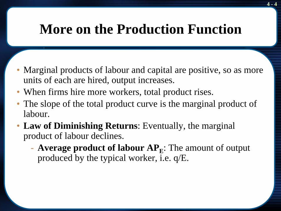
• Marginal products of labour and capital are positive, so as more units of each are hired, output increases.
• When firms hire more workers, total product rises.• The slope of the total product curve is the marginal product of
labour.• Law of Diminishing Returns: Eventually, the marginal
product of labour declines.- Average product of labour APE: The amount of output
produced by the typical worker, i.e. q/E.
4 - 5
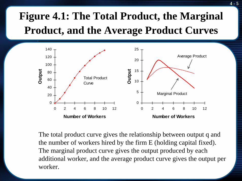
Figure 4.1: The Total Product, the Marginal Product, and the Average Product Curves
0
20
40
60
80
100
120
140
0 2 4 6 8 10 12
Number of Workers
Out
put
Total Product Curve
0
5
10
15
20
25
0 2 4 6 8 10 12
Number of Workers
Out
put
Average Product
Marginal Product
The total product curve gives the relationship between output q and the number of workers hired by the firm E (holding capital fixed). The marginal product curve gives the output produced by each additional worker, and the average product curve gives the output per worker.
4 - 6
Marginal and Average Curves
• Note the following rule:
“The marginal curve lies above the average curve when the average curve is rising, and the marginal curve lies below he average curve when the average curve is falling.”
This implies that “the marginal curve intersects the average curve at the point where the average curve peaks”.
4 - 7
Profit Maximisation
• We assume the objective of the firm is to maximise profits.• The profit function is:
- Profits = pq – wE – rK- Total Revenue = pq- Total Costs = (wE + rk)
• In this chapter it is assumed that the firm is perfectly competitive, i.e. it cannot influence prices of output or inputs (they are assumed constant, irrespective of what the firm does)
• How much E and K should the firm hire?
4 - 8
4.2 The Employment Decision in the Short Run
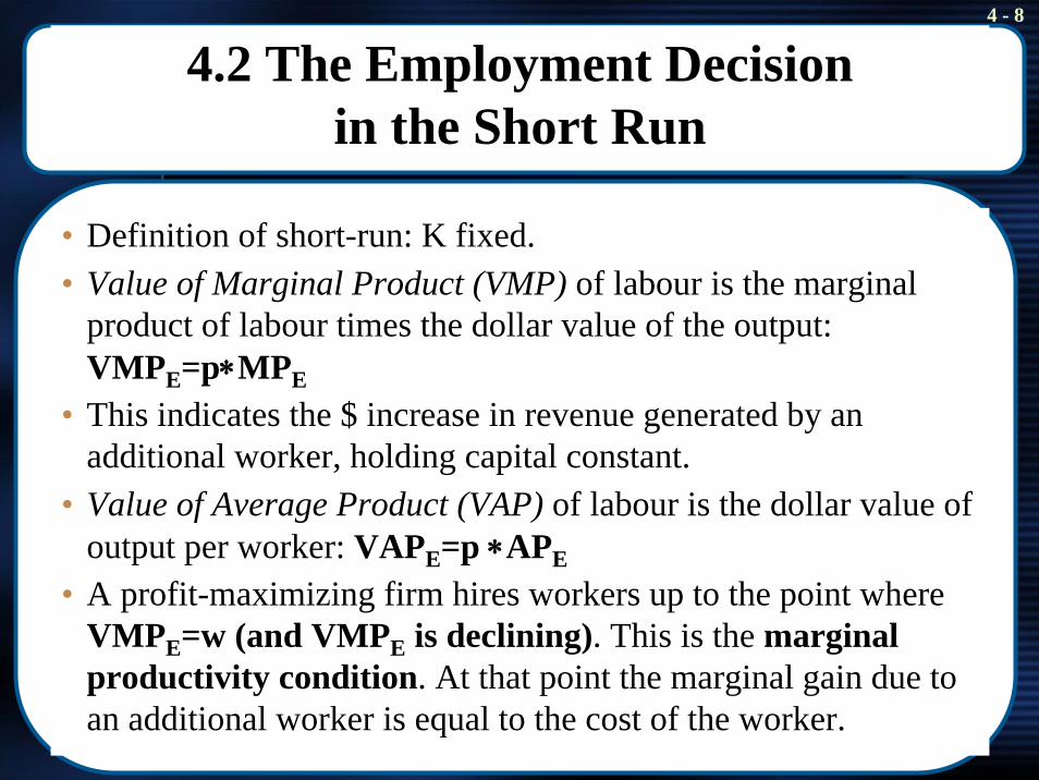
• Definition of short-run: K fixed.• Value of Marginal Product (VMP) of labour is the marginal
product of labour times the dollar value of the output: VMPE=p∗MPE
• This indicates the $ increase in revenue generated by an additional worker, holding capital constant.
• Value of Average Product (VAP) of labour is the dollar value of output per worker: VAPE=p ∗APE
• A profit-maximizing firm hires workers up to the point where VMPE=w (and VMPE is declining). This is the marginal productivity condition. At that point the marginal gain due to an additional worker is equal to the cost of the worker.
4 - 9
Figure 4.2: The Firm's Hiring Decision in the Short-Run
1 4 8
22
38
VMPE
VAPE
Number of Workers
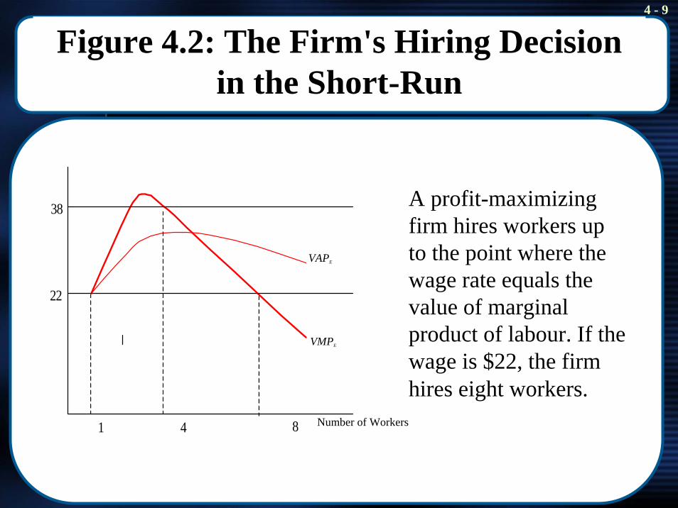
A profit-maximizing firm hires workers up to the point where the wage rate equals the value of marginal product of labour. If the wage is $22, the firm hires eight workers.
4 - 10
The Short-Run Labour Demand Curve
• The short-run demand curve for labour indicates what happens to the firm’s employment as the wage changes, holding capital constant.
• The curve is downward sloping. It is the downward-sloping part of the VMPE curve below its intersection point with the VAPEcurve.
4 - 11
22
18
8 9 12
Figure 4.3: Short-Run Demand Curve for Labour
VMPE
Number of Workers
VMPE
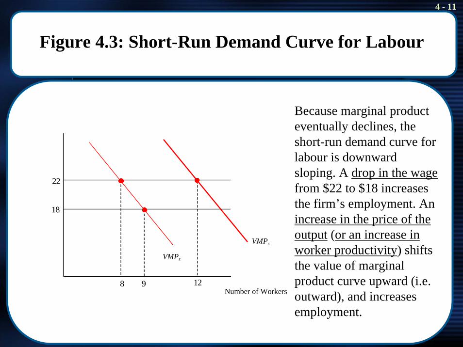
Because marginal product eventually declines, the short-run demand curve for labour is downward sloping. A drop in the wagefrom $22 to $18 increases the firm’s employment. An increase in the price of the output (or an increase in worker productivity) shifts the value of marginal product curve upward (i.e. outward), and increases employment.
4 - 12
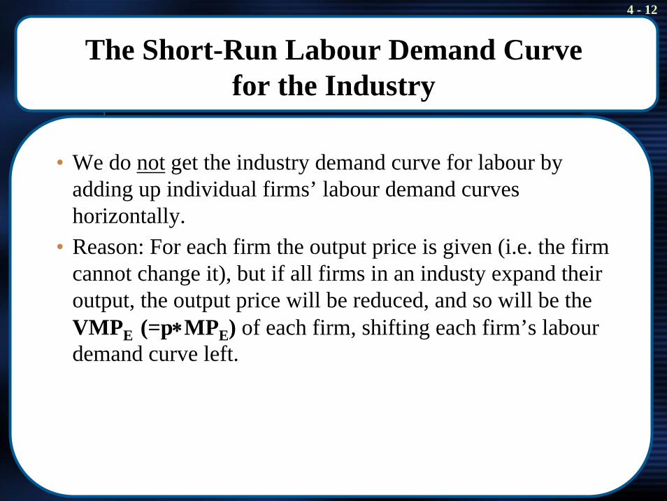
The Short-Run Labour Demand Curvefor the Industry
• We do not get the industry demand curve for labour by adding up individual firms’ labour demand curves horizontally.
• Reason: For each firm the output price is given (i.e. the firm cannot change it), but if all firms in an industy expand their output, the output price will be reduced, and so will be the VMPE (=p∗MPE) of each firm, shifting each firm’s labourdemand curve left.
4 - 13
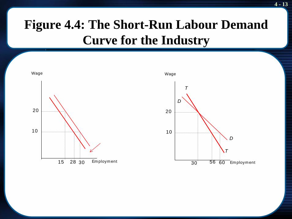
Figure 4.4: The Short-Run Labour Demand Curve for the Industry
20
10
3015
Wage
Employment28
20
10
30 60
Wage
Employment
D
D
56
T
T
4 - 14
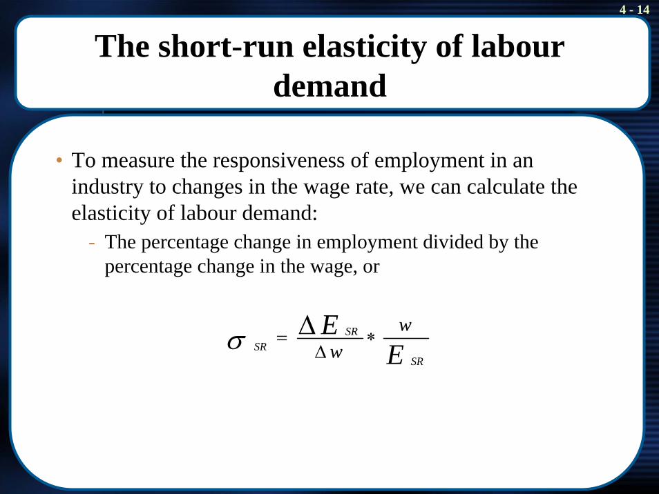
The short-run elasticity of labour demand
• To measure the responsiveness of employment in an industry to changes in the wage rate, we can calculate the elasticity of labour demand:
- The percentage change in employment divided by the percentage change in the wage, or
EE
SR
SRSR
ww
∗Δ
= Δσ
4 - 15
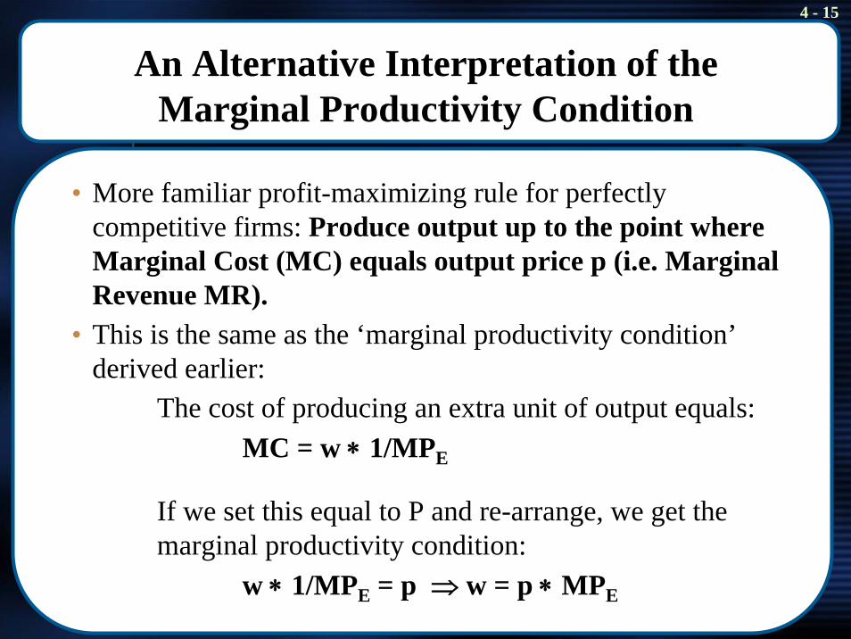
An Alternative Interpretation of the Marginal Productivity Condition
• More familiar profit-maximizing rule for perfectly competitive firms: Produce output up to the point where Marginal Cost (MC) equals output price p (i.e. Marginal Revenue MR).
• This is the same as the ‘marginal productivity condition’ derived earlier:
The cost of producing an extra unit of output equals:MC = w ∗ 1/MPE
If we set this equal to P and re-arrange, we get the marginal productivity condition:
w ∗ 1/MPE = p ⇒ w = p ∗ MPE
4 - 16
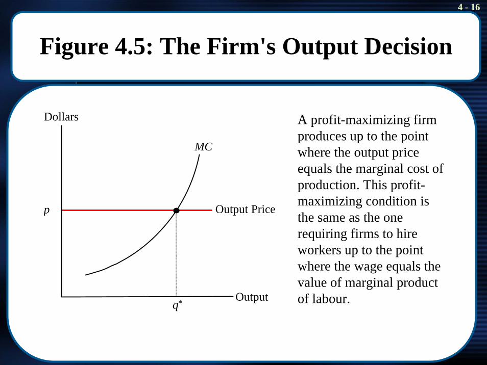
Figure 4.5: The Firm's Output Decision
Output
Dollars
p
q*
MC
Output Price
A profit-maximizing firm produces up to the point where the output price equals the marginal cost of production. This profit-maximizing condition is the same as the one requiring firms to hire workers up to the point where the wage equals the value of marginal product of labour.

4 - 17
Critique of Marginal Productivity Theory
• A common criticism is that the theory bears little relation to the way that employers make hiring decisions.
• Another criticism is that the assumptions of the theory are not very realistic.
• However, employers act as if they know the implications of marginal productivity theory (hence, they try to make profits and remain in business).
4 - 18
4.3 The Employment Decision in the Long Run
• In the long run, the firm maximizes profits by choosing how many workers to hire AND how much plant and equipment to invest in.
• An isoquant describes the possible combinations of labourand capital that produce the same level of output (the curve “ISOlates the QUANTity of output). Isoquants…
- must be downward sloping- do not intersect- that are higher indicate more output- are convex to the origin- have a slope that is the negative of the ratio of the marginal products of
labour and capital. The absolute value of this is called the marginal rate of technical substitution.
4 - 19
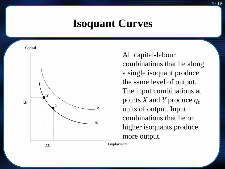
Isoquant Curves
Capital
Employment
q1
q0
X
ΔK
ΔE
Y
All capital-labourcombinations that lie along a single isoquant produce the same level of output. The input combinations at points X and Y produce q0units of output. Input combinations that lie on higher isoquants produce more output.
4 - 20
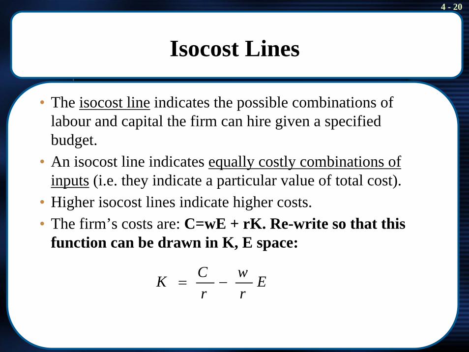
Isocost Lines
• The isocost line indicates the possible combinations of labour and capital the firm can hire given a specified budget.
• An isocost line indicates equally costly combinations of inputs (i.e. they indicate a particular value of total cost).
• Higher isocost lines indicate higher costs.• The firm’s costs are: C=wE + rK. Re-write so that this
function can be drawn in K, E space:
Erw
rCK −=
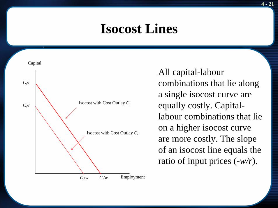
4 - 21
Isocost Lines
Capital
C1/r
Isocost with Cost Outlay C1C0/r
Isocost with Cost Outlay C0
EmploymentC0/w C1/w
All capital-labourcombinations that lie along a single isocost curve are equally costly. Capital-labour combinations that lie on a higher isocost curve are more costly. The slope of an isocost line equals the ratio of input prices (-w/r).
4 - 22
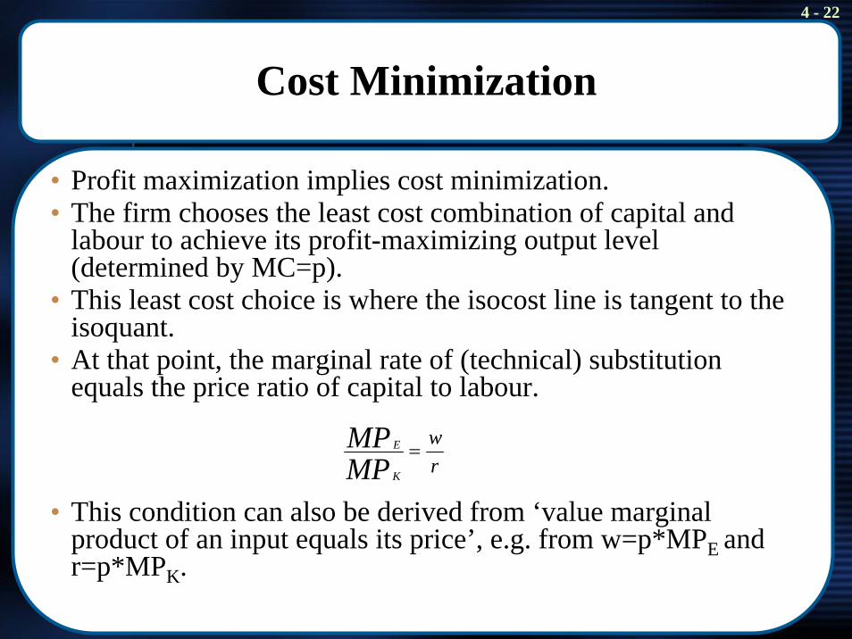
Cost Minimization
• Profit maximization implies cost minimization.• The firm chooses the least cost combination of capital and
labour to achieve its profit-maximizing output level (determined by MC=p).
• This least cost choice is where the isocost line is tangent to the isoquant.
• At that point, the marginal rate of (technical) substitution equals the price ratio of capital to labour.
• This condition can also be derived from ‘value marginal product of an input equals its price’, e.g. from w=p*MPE and r=p*MPK.
rw
MPMP
K
E =
4 - 23
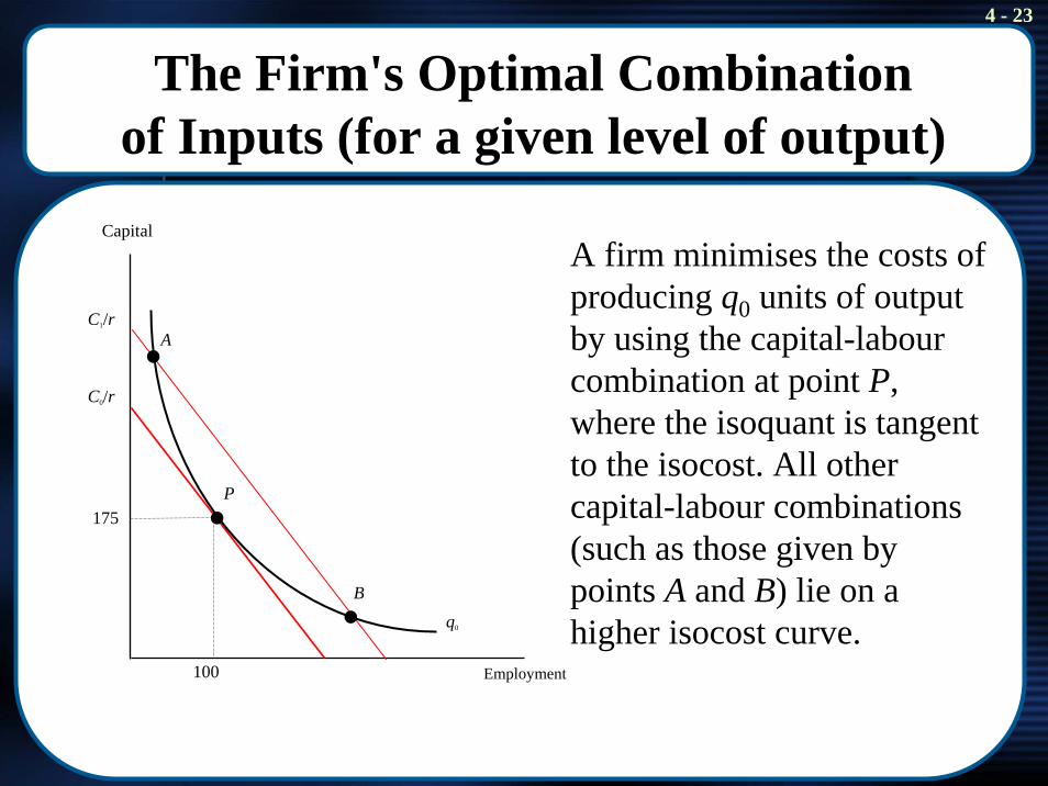
The Firm's Optimal Combination of Inputs (for a given level of output)
Capital
Employment
q0
B
P
A
175
100
C1/r
C0/r
A firm minimises the costs of producing q0 units of output by using the capital-labourcombination at point P, where the isoquant is tangent to the isocost. All other capital-labour combinations (such as those given by points A and B) lie on a higher isocost curve.
4 - 24
4.4 Long Run Demand for Labour
• What happens to the firm’s long-run demand for labour when the wage changes?
• If the wage rate drops, two effects take place that increase thefirm’s labour demand:
- Firm takes advantage of the lower price of labour by expanding production (scale effect).
- Firm takes advantage of the wage change by rearranging its mix of inputs (while holding output constant)(substitution effect).
• If labour is cheaper, the firm will increase its demand for labour. What happens to the demand for capital depends on the relative strength of scale (increased demand for capital) and substitution effects (reduced demand for capital).

4 - 25
Figure 4.9: The Impact of a Wage Reduction, Holding
Constant (Unrealistically!) Initial Cost Outlay at C0
Capital
4025
75
q0
′
RP
C0/r
Wage is w1Wage is w0
q0
A wage reduction flattens the isocost curve. If the firm were to hold the initial cost outlay constant at C0 dollars, the isocost would rotate around C0 and the firm would move from point P to point R. A profit-maximizing firm, however, will not generally want to hold the cost outlay constant when the wage changes, i.e. Figure 4.9 is most likely wrong.
4 - 26
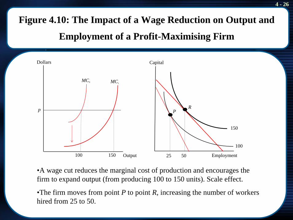
Figure 4.10: The Impact of a Wage Reduction on Output and
Employment of a Profit-Maximising Firm
150100
MC1MC0
p
Dollars
Output
100
150
5025
RP
Capital
Employment
•A wage cut reduces the marginal cost of production and encourages the firm to expand output (from producing 100 to 150 units). Scale effect.
•The firm moves from point P to point R, increasing the number of workers hired from 25 to 50.
4 - 27
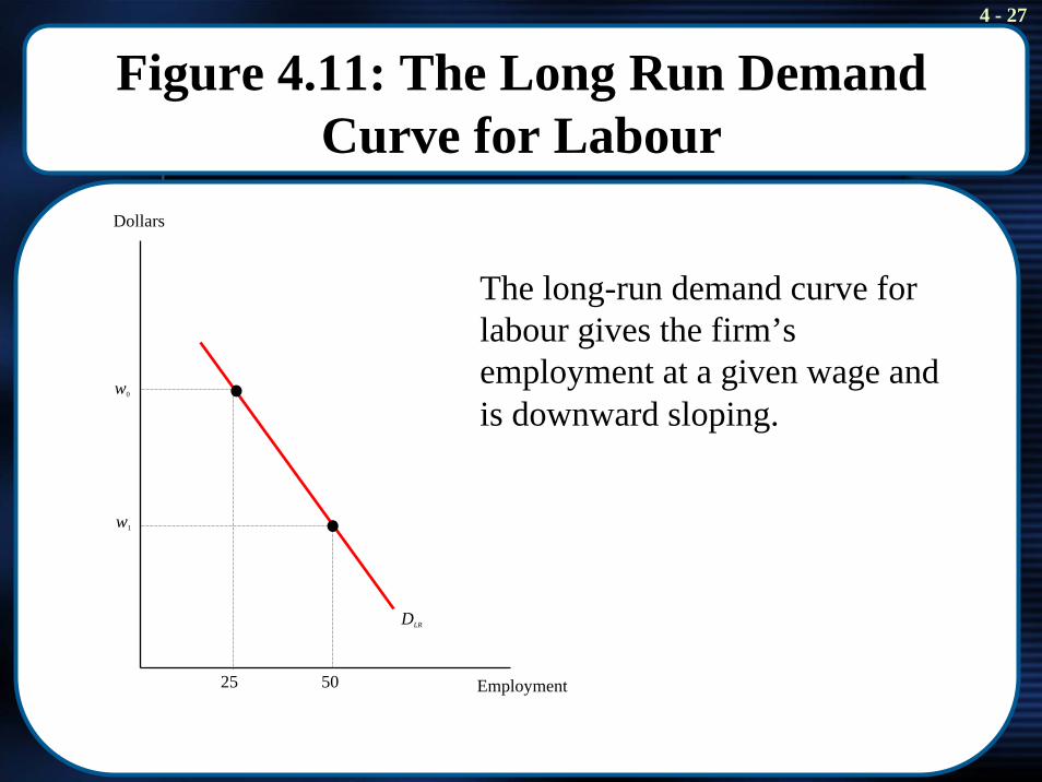
Figure 4.11: The Long Run Demand Curve for Labour
w1
w0
5025
Dollars
Employment
DLR
The long-run demand curve for labour gives the firm’s employment at a given wage and is downward sloping.
4 - 28
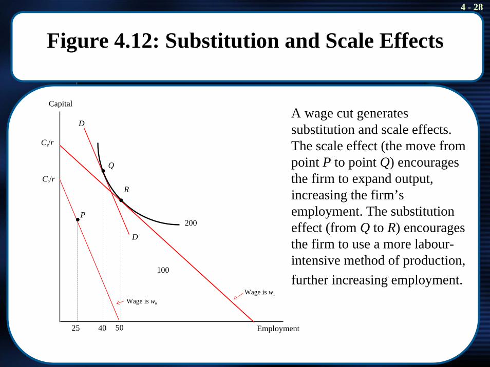
Figure 4.12: Substitution and Scale Effects
100
200
D
R
P
Q
D
5025 40
Capital
Employment
Wage is w1
Wage is w0
C0/r
C1/r
A wage cut generates substitution and scale effects. The scale effect (the move from point P to point Q) encourages the firm to expand output, increasing the firm’s employment. The substitution effect (from Q to R) encourages the firm to use a more labour-intensive method of production, further increasing employment.
4 - 29
Long-run elasticity of labour demand
• In the long run, the firm can take full advantage of the economic opportunities introduced by a change in the wage. As a result, the long-run labour demand curve is more elastic (‘flatter) than the short-run labour demand curve (‘steeper’). See Figure 4.13.
• Wide range of estimates. ‘Consensus’ estimates:- Short-run elasticity between –0.4 and –0.5.- Long-run elasticity around –1.0.
4 - 30
4.5 The Elasticity of Substitution
• When two inputs can be substituted at a constant rate, the two inputs are called perfect substitutes.
• When an isoquant is right-angled, the inputs are perfect complements.
• The substitution effect is very large (infinite) when the two inputs are perfect substitutes. Depending on the slope of the budget line, only one of the inputs will be used in production!
• There is no substitution effect when the inputs are perfect complements (since both inputs are required for production). Input price changes do not alter the input mix.
• The curvature of the isoquant measures elasticity of substitution
4 - 31
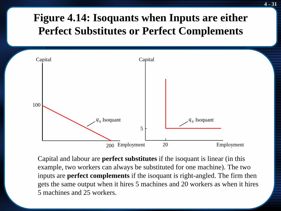
Figure 4.14: Isoquants when Inputs are either Perfect Substitutes or Perfect Complements
Capital
Employment
q 0 Isoquant
100
200
5
20
Capital
Employment
q0 Isoquant
Capital and labour are perfect substitutes if the isoquant is linear (in this example, two workers can always be substituted for one machine). The two inputs are perfect complements if the isoquant is right-angled. The firm then gets the same output when it hires 5 machines and 20 workers as when it hires 5 machines and 25 workers.
4 - 32
Elasticity Measurement
• The more curved the isoquant, the smaller the size of the substitution effect. To measure the curvature of the isoquant we use the elasticity of substitution.
• Intuitively, the elasticity of substitution is the percentage change in capital to labour (a ratio) given a percentage change in the price ratio (wages to real interest):
Percentage change in (K/E) divided by percentage change in (w/r)
• It is a positive number. (w↑ → capital intensity ↑) .
4 - 33
4.6 Application: Affirmative Action and Production Costs - The Importance of Empirical Evidence
• Whether affirmative action (the mandated hiring of certain types of workers, e.g. women, ethnic minorities) improves the profitability of a firm depends on whether or not the firm discriminated before the policy was introduced.
- A) If the firm was discriminating, affirmative action can improve its profitability because discrimination will have shifted the hiring decision away from the cost minimization tangency point on the isoquant. “Discrimination is not profitable”.
- B) If the firm was not discriminating but is forced to adopt affirmative action measures, its costs will increase and its profit will decline. In the extreme case, the firm might go bankrupt.
4 - 34
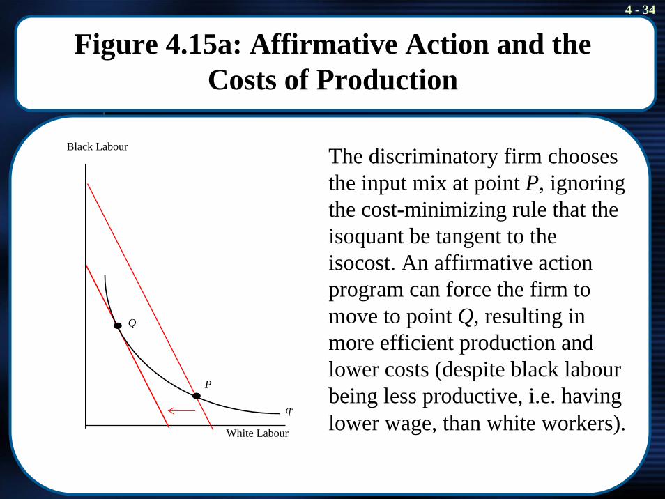
Figure 4.15a: Affirmative Action and the Costs of Production
q*
P
Q
Black Labour
White Labour
The discriminatory firm chooses the input mix at point P, ignoring the cost-minimizing rule that the isoquant be tangent to the isocost. An affirmative action program can force the firm to move to point Q, resulting in more efficient production and lower costs (despite black labourbeing less productive, i.e. having lower wage, than white workers).
4 - 35
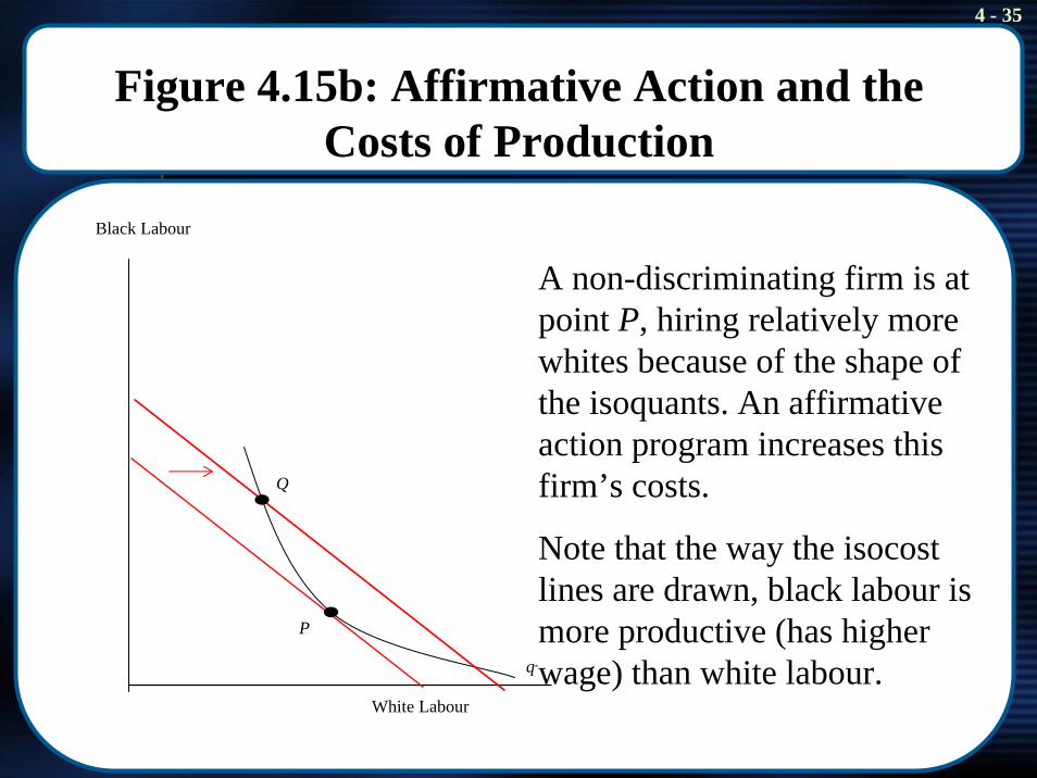
Figure 4.15b: Affirmative Action and the Costs of Production
q*
Q
P
Black Labour
White Labour
A non-discriminating firm is at point P, hiring relatively more whites because of the shape of the isoquants. An affirmative action program increases this firm’s costs.
Note that the way the isocostlines are drawn, black labour is more productive (has higher wage) than white labour.
4 - 36
4.7 Marshall’s Rules of Derived Demand
• Marshall’s famous four rules about factors that generate elastic industry labour demand curves.
• Labour demand in a particular industry is more elastic if:
- Elasticity of substitution is greater.- Elasticity of demand for the firm’s output is greater.- The greater labour’s share in total costs of production.
- But note the qualification mentioned in Note 12, p. 131. - The greater the supply elasticity of other factors of
production (such as capital).
4 - 37
4.8 Factor Demand with Many Inputs
• There are many different inputs (skilled and unskilled labour; old and new machines, natural resources etc.). They can all be incorporated into the production function.
• Cross-elasticity of factor demand: Percentage change in xi / percentage change in wj
- i.e. responsiveness of demand for input i with respect to price of input j.- If the cross-elasticity is positive, the two inputs are said to be substitutes
in production (if it is negative, they are complements).- Unskilled labour and capital usually found to be substitutes, skilled
labour and capital found to be complements. The capital-skill complementarity hypothesis. Policy implications?
4 - 38
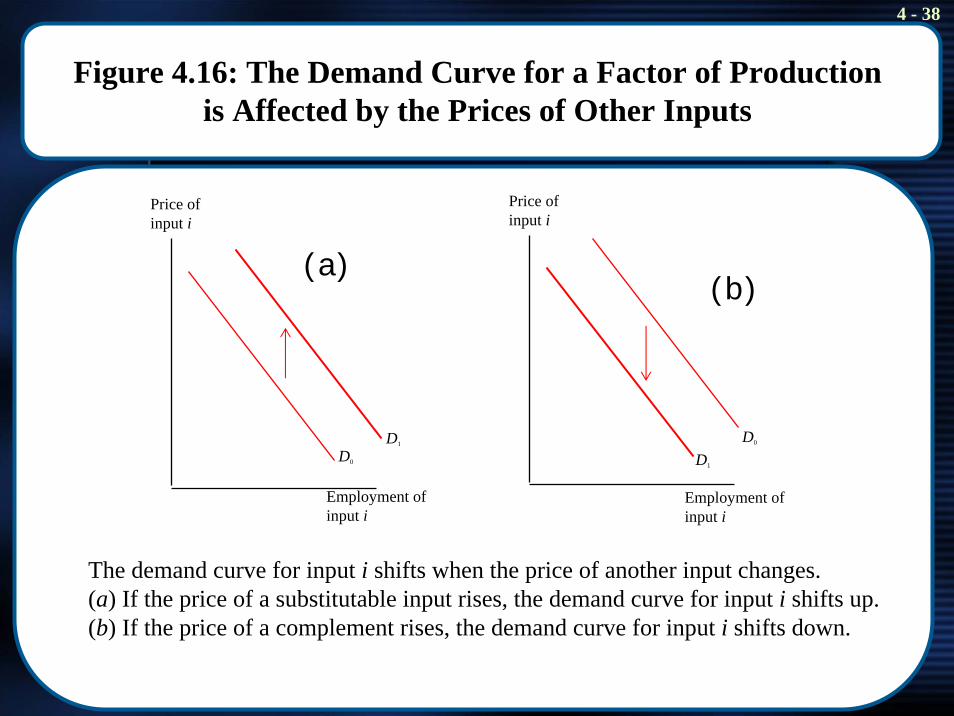
Figure 4.16: The Demand Curve for a Factor of Production is Affected by the Prices of Other Inputs
Price of input i
Employment of input i
D0
Price of input i
Employment of input i
D1 D0
D1
(a)(b)
The demand curve for input i shifts when the price of another input changes. (a) If the price of a substitutable input rises, the demand curve for input i shifts up. (b) If the price of a complement rises, the demand curve for input i shifts down.
4 - 39
4.9 Labour Market Equilibrium(more on this topic in chapter5!)
Dollars
Supply
whigh
w*
ESED E*
wlow
Demand
Employment
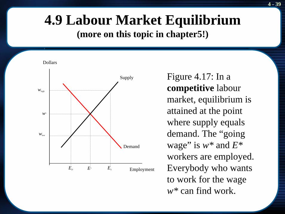
Figure 4.17: In a competitive labourmarket, equilibrium is attained at the point where supply equals demand. The “going wage” is w* and E*workers are employed. Everybody who wants to work for the wage w* can find work.
4 - 40
4.10 Application: The Employment Effects of Minimum Wages (the simple case)
• The ‘standard model’ of the effects of a minimum wage:
- It creates or increases unemployment of the low skilled (some formerly employed people will lose their jobs, other people willbe attracted into the market, but labour demand declines).
- It benefits some employed low skilled workers but disadvantages others.
- The unemployment rate is higher the higher the minimum wage and the more elastic the labour supply and demand curves.
4 - 41
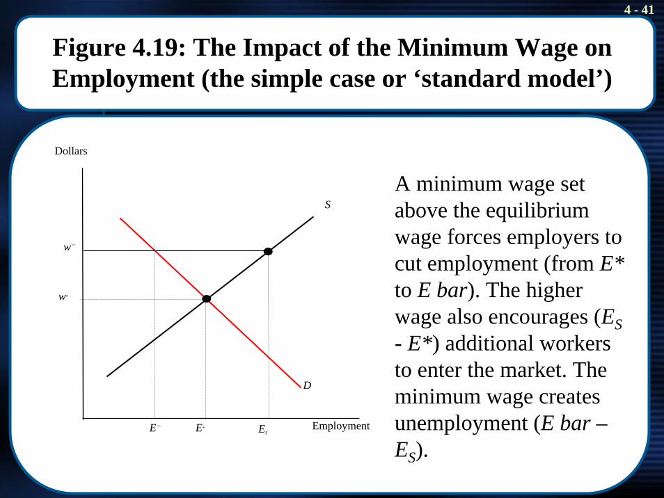
Figure 4.19: The Impact of the Minimum Wage on Employment (the simple case or ‘standard model’)
Dollars
S
D
Employment
w*
w−
ESE*E−
A minimum wage set above the equilibrium wage forces employers to cut employment (from E*to E bar). The higher wage also encourages (ES- E*) additional workers to enter the market. The minimum wage creates unemployment (E bar –ES).
4 - 42
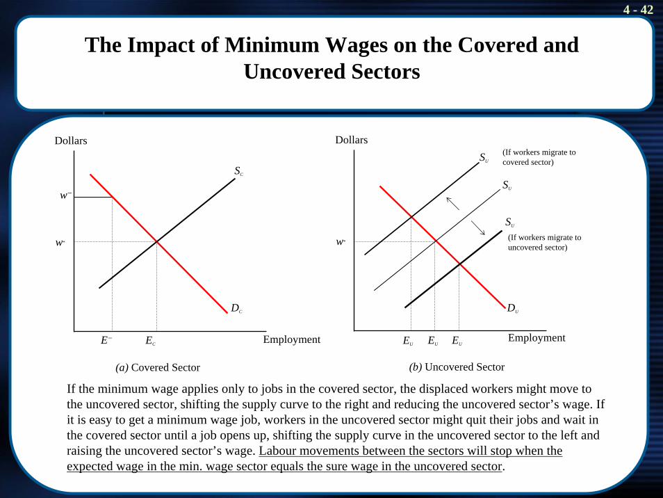
The Impact of Minimum Wages on the Covered and Uncovered Sectors
SU
Dollars Dollars
SC
EmploymentEU EU EUEC Employment
(b) Uncovered Sector
E−
SU
SU
w−
w*w*
DUDC
(If workers migrate to covered sector)
(If workers migrate to uncovered sector)
(a) Covered Sector
If the minimum wage applies only to jobs in the covered sector, the displaced workers might move to the uncovered sector, shifting the supply curve to the right and reducing the uncovered sector’s wage. If it is easy to get a minimum wage job, workers in the uncovered sector might quit their jobs and wait in the covered sector until a job opens up, shifting the supply curve in the uncovered sector to the left and raising the uncovered sector’s wage. Labour movements between the sectors will stop when the expected wage in the min. wage sector equals the sure wage in the uncovered sector.

4 - 43
The Employment Effects of Minimum Wages (the ‘non-standard model’)
• Lots of empirical studies on the impact of minimum wages on employment (often using data on teenagers).
• US findings: minimum wage up, teenage employment down (elasticity between –0.1 and –0.3).
• Some recent studies seem to contradict this ‘consensus’: Imposing a minimum wage might actually increase employment! (5 reasons that might explain this results, pp. 144/5)
- NOTE: In this chapter only the empirical evidence is introduced. A theoretical model that might be able to explain these findings is contained in chapter 5, section 5.8, of the Borjas textbook.
• Some facts from two NZ studies were mentioned in class (Hyslop and Stillman, 2007; Pacheco, 2007). Full references are given in your Course Reading List. A two page handout on the NZ minimum wagewas also provided.
4 - 44
4.11 Adjustment Costs and Labour Demand
• So far our labour demand model assumed that a firm can instantly change the level of employment. This is not the case in reality.
• The expenditures that firms incur as they adjust the size of their workforce are called adjustment costs.
- Variable adjustment costs are associated with the number of workers the firm will hire and fire.
- Fixed adjustment costs do not depend on how many workers the firm is going to hire and fire.
• The two types of adjustment costs will have different implications for firm behaviour.
4 - 45
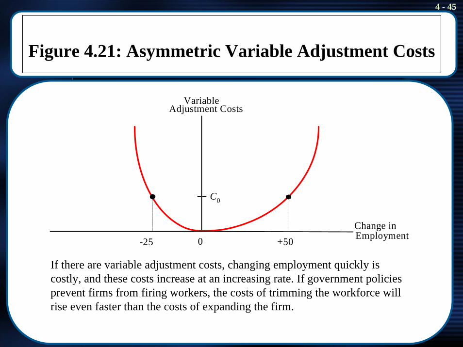
Figure 4.21: Asymmetric Variable Adjustment Costs
Change in
C0
+50-25 Employment0
VariableAdjustment Costs
If there are variable adjustment costs, changing employment quickly is costly, and these costs increase at an increasing rate. If government policies prevent firms from firing workers, the costs of trimming the workforce will rise even faster than the costs of expanding the firm.
4 - 46
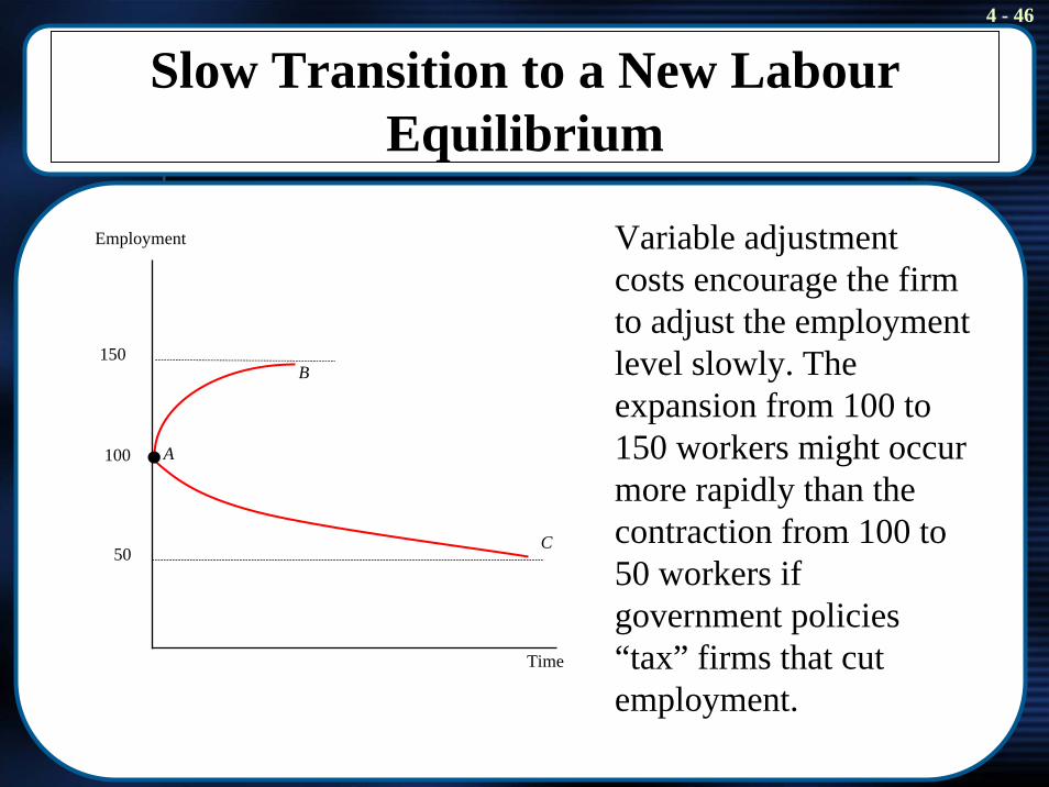
Slow Transition to a New LabourEquilibrium
Employment
B150
A100
C50
Time
Variable adjustment costs encourage the firm to adjust the employment level slowly. The expansion from 100 to 150 workers might occur more rapidly than the contraction from 100 to 50 workers if government policies “tax” firms that cut employment.
4 - 47
Adjustment Costs and Labour Demand
• If there are fixed adjustment costs, they have to be paid whether the firm hires or fires one or many workers.
• The firm faces a cost-benefit situation: Is it profitable to increase the number of workers now (extra revenue) and pay the fixed adjustement costs (extra cost)? Sometimes it will be, sometimes it will not. It depends on whether variable or fixed adjustment costs dominate:
- If fixed adjustment costs are large, employment changes in a firm will either be sudden and large, or they will not occur at all.
- If variable adjustment costs are large (compared to fixed adjustment costs) employment changes are likely to occur slowly.
• Both types of adjustment costs are important in reality. We can say that firms usually take a while to adjust to a new equilibrium when economic circumstances change (6 months to adjust half-way?).

4 - 48
Adjustment Costs and Labour Demand
• There are some other interesting topics in section 4.11 that students should read and try to understand but that are not covered in class:
- The likely impact of employment protecton legislation.- The distinction between workers and hours (including the Theory at
Work piece on ‘work-sharing in Germany’). Increasing fixed costs of employment (p. 152)
- Job creation and job destruction: Lots of it is going on at the same time! This is also the case in NZ:
• In the year to December 2005, there was an average quarterly worker turnover rate of 17.6 percent. By firm size, it was highest in firms with 1-5 employees (19.2%), while firms with 100+ employees had the lowest (15.8%). See Statistics NZ “Linked Employer-Employee Data – December 2005 quarter” (published February 2007, availble on-line).
4 - 49
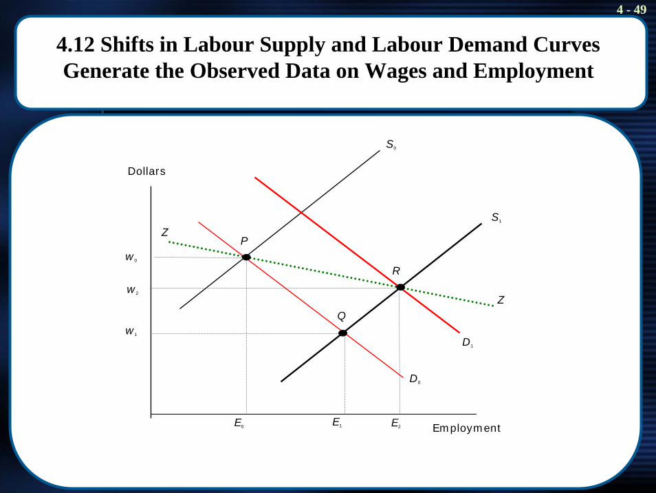
4.12 Shifts in Labour Supply and Labour Demand Curves Generate the Observed Data on Wages and Employment
Dollars
S0
w0
E1E0
D0
Employment
w1
S1
D1
w2
E2
Z
Z
P
Q
R

4 - 50
How to estimate labour demand and labour supply elasticities?
• This is very tricky. The textbook gives an example, which should be of interest to those students that also do, or intend to do, a course in econometrics.
• Essentially, because observed wage and employment data are almost always due to both shifts in the demand and supply curve, empirical economist somehow have to hold constant one curve to estimate the other. This is done in econometrics using the method of instrumental variables. Good instrumental variables are often difficult to find.

4 - 51
End of Chapter 4