LAND SURFACE FEEDBACKS ON THE POST-LANDFALL TROPICAL CYCLONE

CHARACTERISTICS USING THE HURRICANE WEATHER RESEARCH AND

FORECASTING (HWRF) MODELING SYSTEM

A Thesis

Submitted to the Faculty

of

Purdue University

by

Monica Laureano Bozeman

In Partial Fulfillment of the

Requirements for the Degree

of

Master of Science

December 2011

Purdue University

West Lafayette, Indiana

ii

ii

To my husband, Jay, for always believing in me and making me laugh even when times

become difficult.

To Kit and Keisa, who always bring me joy and warm my heart.

iii

iii

ACKNOWLEDGEMENTS

The author would like to thank Dr. Frank Marks Jr. and Dr. S. Gopalakrishnan for the

opportunity to visit the Hurricane Research Division and work with the HRD staff

scientists. Thank you Dr. Xuejin Zhang (HRD/CIMAS) and Dr. Vijay Talapragada

(NOAA/EMC) for assisting with the HWRF model code and data collection. Thank you

to Dr. Kevin Yeh (HRD/CIMAS) for working closely with me on GrADS scripting and

for distributing the diapost program. Thank you to NOAA for starting the Hurricane

Forecast Improvement Project (HFIP) so that I was able to help operational centers with

hurricane research. Thank you to the Developmental Testbed Center (DTC) in Boulder,

CO for making the HWRF model available to the public and educating new users through

annual workshops.

This Study benefitted in parts from the National Science Foundation CAREER grant

(ATM-0847472), Department of Energy-Atmospheric Radiation Measurement (DOE

ARM)-Coupled Cloud and Land Surface Interaction Campaign (CLASIC) (08ER64674),

and from the National Oceanic and Atmospheric Administration (NOAA)-India Ministry

of Earth Sciences (MoES) Interagency Agreement on Tropical Cyclones involving the

Atlantic Oceanographic and Meteorological Laboratory (AOML), India Meteorological

Department (IMD), Indian Institute of Technology (IIT) Delhi, and Purdue University.

iv

iv

TABLE OF CONTENTS

Page

LIST OF TABLES .............................................................................................................. v

LIST OF FIGURES ........................................................................................................... vi

ABSTRACT ...................................................................................................................... xii

CHAPTER 1 INTRODUCTION AND MOTIVATION .................................................... 1

1.1 Introduction................................................................................................................1

References......................................................................................................................12

CHAPTER 2 TS Fay 2008 Case study ............................................................................. 17

2.1 Introduction..............................................................................................................17

2.2 Numerical Model and Experiments .........................................................................19

2.3 Results and Discussion ............................................................................................24

2.3.1 Influence of GFDL Slab versus Noah LSM .....................................................24

2.3.2 Influence of Lake Okeechobee and Florida Everglades ...................................25

2.3.3 Noah Ensemble Runs ........................................................................................31

2.3.4 Revisiting the Noah LSM Intensity Analysis and Mechanisms for Decay ......35

2.3.5 Noah LSM Water Budget .................................................................................38

2.4 Conclusions .............................................................................................................43

References......................................................................................................................46

LIST OF REFERENCES .................................................................................................. 69

APPENDIX: MODIFICATION OF GEOGRAPHY TILES ............................................ 77

VITA ................................................................................................................................. 87

PUBLICATION ................................................................................................................ 89

v

v

LIST OF TABLES

Table .............................................................................................................................. Page

Table 2.1. HWRF model configuration for experiments. ................................................. 52

Table 2.2. LSM model runs with changed surface features. ............................................. 53

Table 2.3. Noah LSM ensemble members. ....................................................................... 55

Appendix Table

Table A.1. USGS Landuse Categories. ............................................................................. 82

Table A.2. Soil Type Categories. ...................................................................................... 83

vi

vi

LIST OF FIGURES

Figure ............................................................................................................................. Page

Figure 1.1. Ensemble track forecasts for TS Fay at (a) 20080816 18Z, (b) 20080817 18Z,

(c) 20080818 18Z, (d) 20080819 06Z............................................................................... 16

Figure 2.1. Melbourne (KMLB) radar images of TS Fay eye development: (a)0634Z Aug

19 (b) 0935Z Aug 19 (c) 1811Z Aug 19 (d) 0058Z Aug 20 (e) 0258Z Aug 20. .............. 51

Figure 2.2. USGS landuse categories of the dominant 18 landuse categories in Florida,

produced by the 1 km AVHRR data from April 1992 until March 1993. Image obtained

from <http://fcit.usf.edu/florida/maps/land_use/land_use.htm> and modified to indicate

locations of interest.. ......................................................................................................... 54

Figure 2.3. HWRF model forecast track errors (FTE): (a) GFDL Slab versus Noah (b)

GFDL Slab land changes (SW, SL, SG) versus Noah LSM land changes (NW, NL, NG)

(c) Noah LSM ensemble members (NW, NL, NG, NY, NM, N6B, N6A). Fay best track

(BT) forecast is indicated with the thck black line. .......................................................... 56

Figure 2.4. Along-track maximum winds (kt) for 00Z Aug 19 until 06Z Aug 20: (a)

GFDL Slab versus Noah LSM (b) Noah LSM land changes (c) Noah LSM ensemble.

Fay‟s Florida landfall on Cape Romano at 09Z on August 19th

2008 is indicated by the

black line. .......................................................................................................................... 57

Figure 2.5. Same as Figure 2.4 but for mean sea level pressure (mb, MSLP).................. 58

vii

vii

Figure ............................................................................................................................. Page

Figure 2.6. Noah (top) and GFDL Slab (bottom) LSM land changes 10 meter wind

differences (kt) from 00Z Aug 19 until 06Z Aug 20. ....................................................... 59

Figure 2.7. Dotted line (A-B) indicates the location of the cross section for the GFDL

Slab (S) and Noah (N) LSM tracks. The large circles along each track indicate the

position of the storm at the time of the cross-section images (18Z Aug 19). ................... 60

Figure 2.8. Noah (top) and GFDL Slab (bottom) LSM land changes horizontal cros

section plots for the magnitude of the 10 meter winds (left), MSLP (middle), and surface

latent heat flux (right) at 18Z Aug 19, along the cross section line A-B shown in Figure

2.7...................................................................................................................................... 61

Figure 2.9. Far Left: Noah (top) and GFDL Slab (bottom) LSM accumulated rainfall (mm)

from 00Z Aug 19 until 06Z Aug 20. Right: Accumulated rainfall differences for land

surface changes for the same time period. ........................................................................ 62

Figure 2.10. Left: Noah No Ocean (NNO) forecast track and accumulated rainfall (mm).

Right: No Ocean rainfall accumulation and track difference from the Noah default (N). 63

Figure 2.11. Noah No Ocean (NNO) difference in 10 meter wind magnitude from the

Noah default (N). .............................................................................................................. 64

Figure 2.12. Noah LSM ensemble accumulated rainfall (mm) from 00Z Aug 19 until 06Z

Aug 20. .............................................................................................................................. 65

Figure 2.13. Noah only ocean tests for 00Z Aug 19 until 06Z Aug 20: (a) MSLP (mb), (b)

10 meter maximum winds (kt), (c) tangential latent heat flux (W/m2), (d) tangential

sensible heat flux (W/m2), (e) tangential frictional stress (kg/m/s

2). Fay‟s Florida landfall

on Cape Romano at 09Z on Augus 19th

2008 is indicated by the black line. ................... 66

viii

viii

Figure 2.14. Radius-height cross-section of the Noah LSM ocean tests All Ocean (top),

Default (middle) and No Ocean (bottom) secondary circulation vectors, radial moisture

convergence (kg/kg/s) with vertical moisture divergence (kg/kg*m/s, left) and radial

moisture advection (kg/kg/s) with vertical moisture flux (g/m2s, right) at 18Z Aug 19. . 67

Figure 2.15. Azimuth-radius horizontal plane of Noah LSM ocean tests All Ocean (top),

Default (middle) and No Ocean (bottom) horizontal gradient of the vertical moisture flux

(g/m2s) at 2000 m (left) and 70 m (right) at 18Z Aug 19. ................................................ 68

Appendix Figure

Figure A.1. Original USGS landuse (top), Top Soil Type (middle) and Bottom Soil Type

(lower) of Southern Florida. Boxed locations indicate regions where geography tiles will

be altered. .......................................................................................................................... 85

Figure A.2. Same as Figure A.1, but for changed geography tile values. ........................ 86

ix

ix

LIST OF ABBREVIATIONS

TC or TCs Tropical Cyclone(s)

TS Tropical Storm

DTC Developmental Testbed Center, located in Boulder, CO

HWRF Hurricane Weather Research and Forecasting Model

WRF Weather Research and Forecasting Model

PBL Planetary Boundary Layer

GFDL Geophysical Fluid Dynamics Laboratory

LSM or LSMs Land Surface Model(s)

NOAH or Noah

NOAH is an acronym of acronyms for the contributing offices

that helped develop the land surface model. N=NCEP,

O=Oregon State University (Dept. of Atmospheric Sciences),

A=Air Force (AF Weather Agency and AF Research Lab),

H=NWS Hydrologic Research Lab

NOAA National Oceanic and Atmospheric Administration

HFIP Hurricane Forecast Improvement Project

NCAR, RAL National Center for Atmospheric Research, Research

Applications Laboratory

NESDIS, STAR National Environmental Satellite, Data and Information

Service, Center for Satellite Applications and Research

ESRL Earth System Research Laboratory

NWS National Weather Service

NHC NOAA National Hurricane Center, located in Miami, FL

x

x

NCEP National Center for Environmental Prediction

EMC NCEP Environmental Modeling Center, located in Camp

Springs, MD

AOML-HRD

NOAA Atlantic Oceanographic and Meteorological

Laboratory, Hurricane Research Division, located in Miami,

FL

NRL Naval Research Laboratory

HWRFx Experimental HWRF developed by the AOML-HRD

NMM Non-hydrostatic Mesoscale Model

GFS Global Forecast System

POM Princeton Ocean Model

SST Sea Surface Temperature

USGS United States Geological Survey

NASA National Aeronautics and Space Administration

MODIS NASA Moderate Resolution Imaging Spectroradiometer

ET Extratropical Transition

NWP Numerical Weather Prediction

ABL Atmospheric Boundary Layer

WPS WRF Pre-processing System

FTE Forecast Track Error

MSLP Mean Sea Level Pressure described in millibars

MYJ Mellor-Yamada-Janjic PBL parameterization in the WRF

xi

xi

model

YSU Yonsei University PBL scheme in the WRF model

MFC Moisture Flux Convergence

xii

xii

ABSTRACT

Bozeman, Monica L. M.S., Purdue University, December 2011. Land Surface Feedbacks

on the Post-landfall Tropical Cyclone Characteristics using the Hurricane Weather

Research and Forecasting (HWRF) Modeling System. Major Professors: Dev Niyogi,

Michael Baldwin.

While tropical cyclones (TCs) usually decay after landfall, Tropical Storm Fay (2008)

initially developed a storm central eye over South Florida by anomalous intensification

overland. Unique to the Florida peninsula, are Lake Okeechobee and the Everglades

which may have provided a surface feedback as the TC tracked near these features

around the time of peak intensity. Analysis is done with the use of an ensemble model-

based approach with the Developmental Testbed Center (DTC) version of the Hurricane

WRF (HWRF) model using an outer domain and a storm centered moving nest with 27

km and 9 km grid spacing respectively. Choice of land surface parameterization and

small-scale surface features may influence TC structure, dictate the rate of TC decay, and

even the anomalous intensification after landfall in model experiments. Results indicate

that the HWRF model track and intensity forecasts are sensitive to three features in the

model framework: land surface parameterization, initial boundary conditions and choice

of Planetary Boundary Layer (PBL) scheme. Land surface parameterizations such as the

Geophysical Fluid Dynamics Laboratory (GFDL) Slab and Noah land surface models

(LSMs) dominate the changes to storm track, while initial conditions and PBL schemes

xiii

xiii

cause the largest changes to the TC intensity overland. Land surface heterogeneity in

Florida from removing surface features in model simulations, show a small role in

forecast intensity change with no substantial alterations to TC track.

1

1

CHAPTER 1 INTRODUCTION AND MOTIVATION

1.1 Introduction

Since the year 2005 when Hurricane Katrina devastated the Louisiana coast, more

and more attention has been drawn to hurricanes from both the public and atmospheric

scientists. Tropical forecasting is in a relatively undeveloped stage of observations and

research when compared to midlatitude forecasting, so certain aspects about the core

structure and dynamics are still unknown, therefore, intensity forecasts are consistently

stricken with errors and bias (Laing and Evans 2010). Lack of knowledge about tropical

systems is mostly due to the deficiency of observation network infrastructures over the

ocean where these systems spend most of their lifecycle (Rhome and Raman 2010).

Therefore, tropical research is mainly dependent on satellite observations, sensors, and

other creative ways to obtain these critical data (Laing and Evans 2010; Marks and Shay

1997).

To better understand the inner dynamics of TCs and address forecasting issues, the

National Oceanic and Atmospheric Administration (NOAA) organized the Hurricane

Forecast Improvement Project (HFIP), which lays out a 10-year plan to improve the

reliability and accuracy of the one to five day tropical cyclone forecasts. Starting in 2007,

HFIP major goals include reducing errors of hurricane track and intensity forecasts by 20%

2

2

in the five years and by 50% in the next 10 years. The HFIP project allows for

collaboration of the NOAA‟s operational centers, test-bed centers and academia

including the National Center for Atmospheric Research (NCAR)‟s Research

Applications Laboratory (RAL), National Environmental Satellite, Data and Information

Service (NESDIS)‟s Center for Satellite Applications and Research (STAR) – formerly

the Office of Research and Applications (ORA), Earth System Research Laboratory

(ESRL), Geophysical Fluid Dynamics Laboratory (GFDL), Developmental Testbed

Center (DTC), National Weather Service (NWS) National Hurricane Center (NHC),

NWS/NCEP Environmental Modeling Center (EMC), Atlantic Oceanographic and

Meteorological Laboratory Hurricane Research Division (AOML-HRD), and the US

Naval Research Laboratory (NRL) to share their research to meet these goals. Achieving

these goals will lead to greater confidence in hurricane forecasts and may be able to

increase forecast lead times to affected forecast areas to reduce tropical cyclone damage

and loss of life.

To fulfill the need for the US‟s next-generation hurricane model forecasting

problems, the Hurricane Weather Research and Forecasting system (HWRF) was

developed by the EMC with collaboration from the GFDL and the University of Rhode

Island (Bao et al. 2010 ; Gopalakrishnan et al. 2010). HWRF model development started

in 2002 and later became operational at the HPC and EMC in 2007 and subsequently at

the AOML-HRD, which uses HWRF operational and experimentally (HWRFx,

Gopalakrishnan et al. 2011) implementing a configuration with increased horizontal

resolution and an additional inner moving nest. A community version of the HWRF was

released to the public and academia by the DTC in late March of 2010 (Gopalakrishnan

et al. 2010).

3

3

The HWRF is a two-way coupled ocean-atmospheric model based on the NMM

(Non-hydrostatic Mesoscale Model) core of the Weather Research and Forecasting (WRF)

model, for the prediction of hurricanes and tropical systems. Until recently, the leading

operational hurricane model was the GFDL hurricane model from the Geophysical Fluid

Dynamics Laboratory in Princeton New Jersey (Kurihara et al. 1998) which was used as

the baseline for HWRF‟s predictive abilities. Both models incorporate a vortex relocation

system, which removes the initial vortex from the Global Forecast System (GFS) analysis

fields and replaces this vortex with a high-resolution “model consistent” vortex (Liu et al.

2006; Gopalakrishnan et al. 2011, 2010). In addition, both models are coupled to the

Princeton Ocean Model (POM) with loop current initialization to include the effect of

ocean water churning underneath the hurricane center and produce the “cold wake” of a

hurricane as it travels through an ocean basin. This cooling of the ocean surface beneath a

tropical cyclone is an important feature since it severely reduces TC intensity due to lack

of warm SSTs fueling the system. Both models include a large parent domain with a

high-resolution vortex-following inner nest that is centered on the calculated vortex

center and therefore is specific to each tropical cyclone.

However, the newly operational HWRF model also includes additional

components to surpass the GFDL hurricane model‟s intensity forecasts due to its

advanced model physics for high-resolution forecasting, cycling of the model‟s

previously adjusted forecast vortex, and continuous meteorological data assimilation of

“TC Vitals” (Liu et al. 2006; Gopalakrishnan et al. 2010) to improve the 3-D structure of

the TC vortex. TC Vital files are comprised of meteorological data from satellites, buoys,

and data retrieved from hurricane hunter missions

4

4

(http://www.noaanews.noaa.gov/stories2007/s2885.htm). The GFDL method of vortex

initialization involves using a “bogus” vortex (2-D axi-symmetric synthetic vortex) at

each model forecast time. The current operational forecasting configuration includes two

domains: the parent domain uses a 27 km horizontal model resolution and 9 km

resolution in the inner nest.

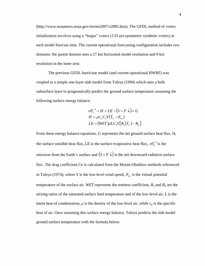
The previous GFDL hurricane model (and current operational HWRF) was

coupled to a simple one-layer slab model from Tuleya (1994) which uses a bulk

subsurface layer to prognostically predict the ground surface temperature assuming the

following surface energy balance:

aLse

vaLep

L

RTRVLCWETLE

TVCcH

GFSLEHT

4

From these energy balance equations, G represents the net ground surface heat flux, H,

the surface sensible heat flux, LE is the surface evaporative heat flux, 4

LT is the

emission from the Earth‟s surface and FS is the net downward radiative surface

flux. The drag coefficient Ce is calculated from the Monin-Obukhov methods referenced

in Tuleya (1974), where V is the low-level wind speed, va is the virtual potential

temperature of the surface air. WET represents the wetness coefficient, Rs and Ra are the

mixing ratios of the saturated surface land temperature and of the low-level air, L is the

latent heat of condensation, ρ is the density of the low-level air, while cp is the specific

heat of air. Once assuming this surface energy balance, Tuleya predicts the slab model

ground surface temperature with the formula below:

5

5

21

/

:

4

ss

ss

LL

cd

where

dc

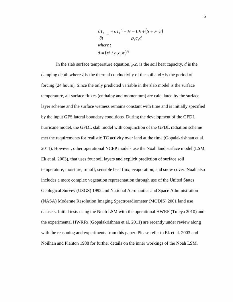
FSLEHT

t

T

In the slab surface temperature equation, ρscs is the soil heat capacity, d is the

damping depth where λ is the thermal conductivity of the soil and τ is the period of

forcing (24 hours). Since the only predicted variable in the slab model is the surface

temperature, all surface fluxes (enthalpy and momentum) are calculated by the surface

layer scheme and the surface wetness remains constant with time and is initially specified

by the input GFS lateral boundary conditions. During the development of the GFDL

hurricane model, the GFDL slab model with conjunction of the GFDL radiation scheme

met the requirements for realistic TC activity over land at the time (Gopalakrishnan et al.

2011). However, other operational NCEP models use the Noah land surface model (LSM,

Ek et al. 2003), that uses four soil layers and explicit prediction of surface soil

temperature, moisture, runoff, sensible heat flux, evaporation, and snow cover. Noah also

includes a more complex vegetation representation through use of the United States

Geological Survey (USGS) 1992 and National Aeronautics and Space Administration

(NASA) Moderate Resolution Imaging Spectroradiometer (MODIS) 2001 land use

datasets. Initial tests using the Noah LSM with the operational HWRF (Tuleya 2010) and

the experimental HWRFx (Gopalakrishnan et al. 2011) are recently under review along

with the reasoning and experiments from this paper. Please refer to Ek et al. 2003 and

Noilhan and Planton 1988 for further details on the inner workings of the Noah LSM.

6

6

While great strengthening can occur in TCs over ocean, at landfall, tropical

systems usually weaken and decay due to a drastic change in surface characteristics. Only

a few cases of overland tropical storm reintensification have been observed and

documented for the Atlantic storms in recent years including TCs Erin (2007) (Arndt et

al. 2009; Monteverdi and Edwards 2010; Monteverdi and Edwards 2008; Evans et al.

2010), Danny (1997) (Bassill and Morgan 2006), Fran (1996) (Kehoe et al. 2010; Rhome

and Raman 2010) and David (1979) (Bosart and Lackmann 1995). According to the cited

studies and observations, the overland reintensification of TCs Danny (1997) and David

(1979) was determined to be caused by experiencing self-development and a combination

of factors usually favorable for extratropical intensification; despite that the surrounding

environment and storm structures both exhibited tropical characteristics. However,

evidence is shown by the authors that TCs Erin (2007) and Fran (1996) were assisted

with redevelopment by the moist ground surface below the storm, which allowed for the

ingestion of surface latent heat to fuel the system similar to oceanic interactions. These

findings for TCs Erin and Fran also follow the thinking of Emanuel et al. (2008) and

Chang et al. (2009) which studied the postlandfall redevelopment of tropical systems

through a moist landsurface feedback in Northern Australia and the Indian monsoon

region respectively. Due to the various processes described as means for redevelopment

or intensification, it is necessary to review the differences between the typical structures

and characteristics for a tropical system and a midlatitude or extratropical weather

system.

7

7

Tropical storms are quite different from their midlatitude counterparts that

regularly affect the weather of the Northern and Southern hemispheres, and their

differential characteristic have been documented in many studies (eg. Bosart and Bartlo

1991). Necessary conditions for TC genesis that must be present, yet does not guarantee

formation include: (1) warm SSTs (at least 26° C), (2) formation within 5° latitude from

the equator, (3) low vertical wind shear, (4) moisture available in the mid-troposphere,

(5) unstable conditions, and (6) a pre-existing disturbance (Laing and Evans 2010).

Tropical storm genesis is said to have occurred once the sustained surface wind speed

(calculated as the one minute average of the 10 meter wind in the US) of a tropical

system exceeds 17 m/s. In addition, the system must be characterized as self-sustaining to

continue to remain a coherent system regardless of external forcing (Laing and Evans

2010). After initial development, a TC is maintained through taking in heat energy from

high ocean temperatures and expelling heat in the cold temperatures of the upper

troposphere. Extratropical cyclones on the other hand, obtain their energy from the

horizontal temperature contrasts in the atmosphere otherwise known as “baroclinic

effects” (Monteverdi and Edwards 2010). Once fully organized, a tropical (midlatitude)

system is characterized by a compact (expansive) symmetrical (asymmetrical) wind and

precipitation structure with stronger (weaker) winds near the surface that decrease

(increase) with height (Laing and Evans 2010; Evans and Hart 2003). Due to the

characteristic vertical wind profile of a tropical cyclone and a midlatitude system, the

thermal wind balance equation can determine the temperature of the tropospheric

anomaly T and therefore why tropical systems are considered “warm-cored” and

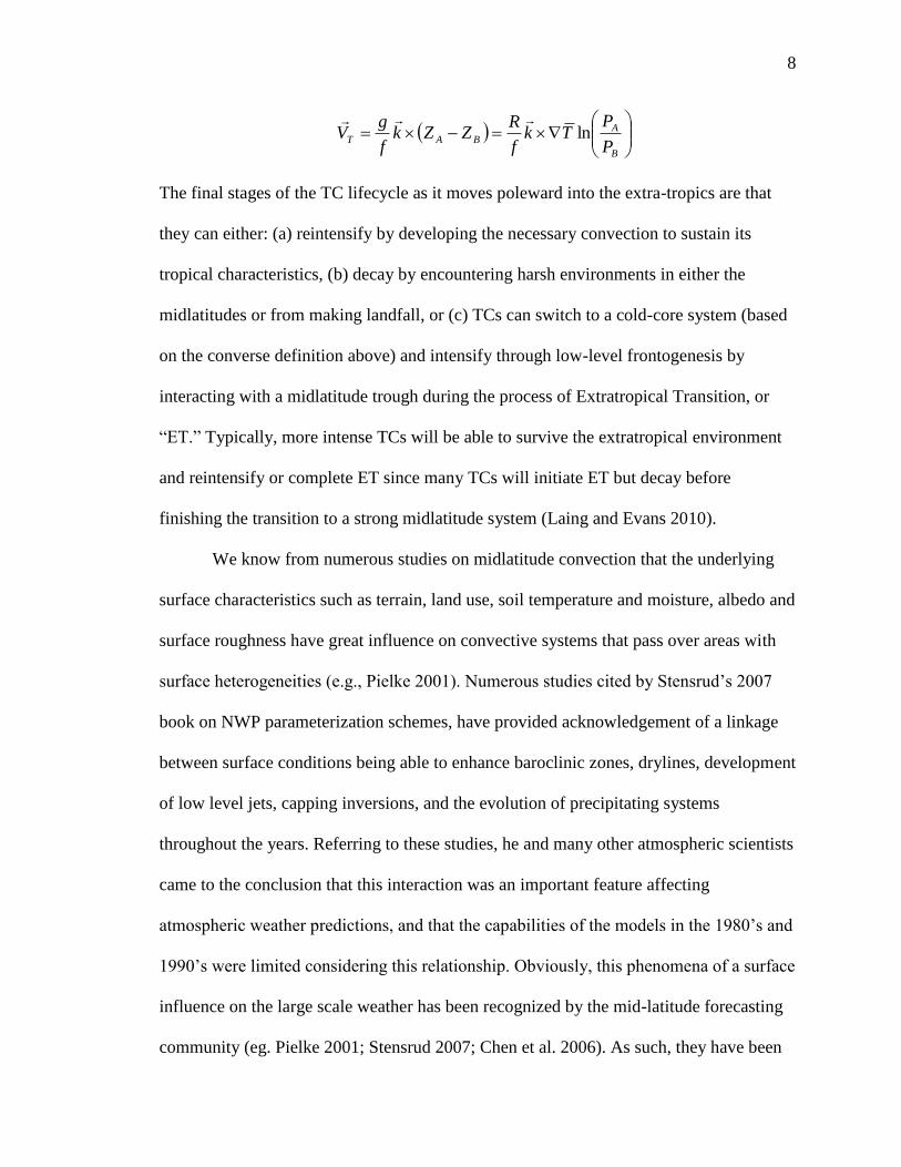
midlatitude or extratropical systems are referred to as “cold-cored.”

8

8

B

ABAT

P

PTk

f

RZZk

f

gV ln

The final stages of the TC lifecycle as it moves poleward into the extra-tropics are that

they can either: (a) reintensify by developing the necessary convection to sustain its

tropical characteristics, (b) decay by encountering harsh environments in either the

midlatitudes or from making landfall, or (c) TCs can switch to a cold-core system (based

on the converse definition above) and intensify through low-level frontogenesis by

interacting with a midlatitude trough during the process of Extratropical Transition, or

“ET.” Typically, more intense TCs will be able to survive the extratropical environment

and reintensify or complete ET since many TCs will initiate ET but decay before

finishing the transition to a strong midlatitude system (Laing and Evans 2010).

We know from numerous studies on midlatitude convection that the underlying

surface characteristics such as terrain, land use, soil temperature and moisture, albedo and

surface roughness have great influence on convective systems that pass over areas with

surface heterogeneities (e.g., Pielke 2001). Numerous studies cited by Stensrud‟s 2007

book on NWP parameterization schemes, have provided acknowledgement of a linkage

between surface conditions being able to enhance baroclinic zones, drylines, development

of low level jets, capping inversions, and the evolution of precipitating systems

throughout the years. Referring to these studies, he and many other atmospheric scientists

came to the conclusion that this interaction was an important feature affecting

atmospheric weather predictions, and that the capabilities of the models in the 1980‟s and

1990‟s were limited considering this relationship. Obviously, this phenomena of a surface

influence on the large scale weather has been recognized by the mid-latitude forecasting

community (eg. Pielke 2001; Stensrud 2007; Chen et al. 2006). As such, they have been

9

9

working to improve land surface parameterizations of the physical properties of the soil

and vegetation into coupled and uncoupled land surface models. These improved LSMs

have recently become tested and implemented in countless NCEP weather models, and

results show forecasts that more closely match observations (eg. Ek et al. 2003; Chen et

al. 2006). In addition, new datasets for improved land representation have been

developed for input in land surface and numerical models such as the NASA Global Land

Data Assimilation System (GLDAS), Land Information System (LIS), NCAR High

Resolution Land Data Assimilation System (HRLDAS, Chen et al. 2006) and NCEP

North-American Land Data Assimilation System (NLDAS). Pielke‟s 2001 paper does a

reasonable job attempting to show a link between surface moisture and heat fluxes with

cumulus convective rainfall through a review of a massive number of atmospheric-land

surface studies. According to Pielke (2001) the precipitation rate and type influence how

water can be distributed between runoff, infiltration to the soil, and the interception of

water on plant surfaces. Relating this statement to the large amounts of precipitation

associated with TCs at landfall, we can acknowledge that vegetation, soil and landuse

type, the inherent thermal and moisture properties, and the spatial distribution of these

land surface elements will have an impact or feedback on the latent heat flux which

drives the intensity of the tropical system and rainfall patterns as the TC encounters and

continues to travel over land. Since TCs spend most of their time over oceans, the

concept is recognized but still a subject with much uncertainty partly due to the low

occurrence of far inland tracks retaining tropical characteristics and the difficulty of

obtaining ground and atmospheric boundary layer (ABL) observations in a high surface

wind environment (Knupp et al. 2005), an attribute of TCs at landfall. Therefore, studies

10

10

focused on establishing an influence of the land surface properties on TC landfall and

decay are usually through idealized modeling experiments (eg. Kimball 2004; Dastoor

and Krishnamurti 1991; Emanuel et al. 2008; Wong and Chan 2007; Tuleya et al. 1984;

Tuleya and Kurihara 1978; Tuleya 1994). Yet some are fortunate enough to study the

somewhat rare opportunities when TCs make landfall or travel over observationally

dense regions (eg. Arndt et al. 2009; Kehoe 2010; Knupp et al. 2005). According to

Marks and Shay (1997), a synthesis of observations, theory and numerical modeling is

needed to progress forecasting of TC intensity and storm structural changes during

landfall.

In recent years, hurricane research has placed increased attention on improving

model track and intensity forecasts of TCs with vortex following domains, vortex and

ocean initialization with high resolution ocean data and a synthetic or “bogus” vortex

during a cold-start to correct the simulated storm intensity (Gopalakrishnan et al. 2011;

Singh et al. 2005). While TC track forecasts in ocean basins have been significantly

improved in all hurricane models, many models have difficulty converging on an

overland track as there is uncertainty with the complexity of the land-atmosphere

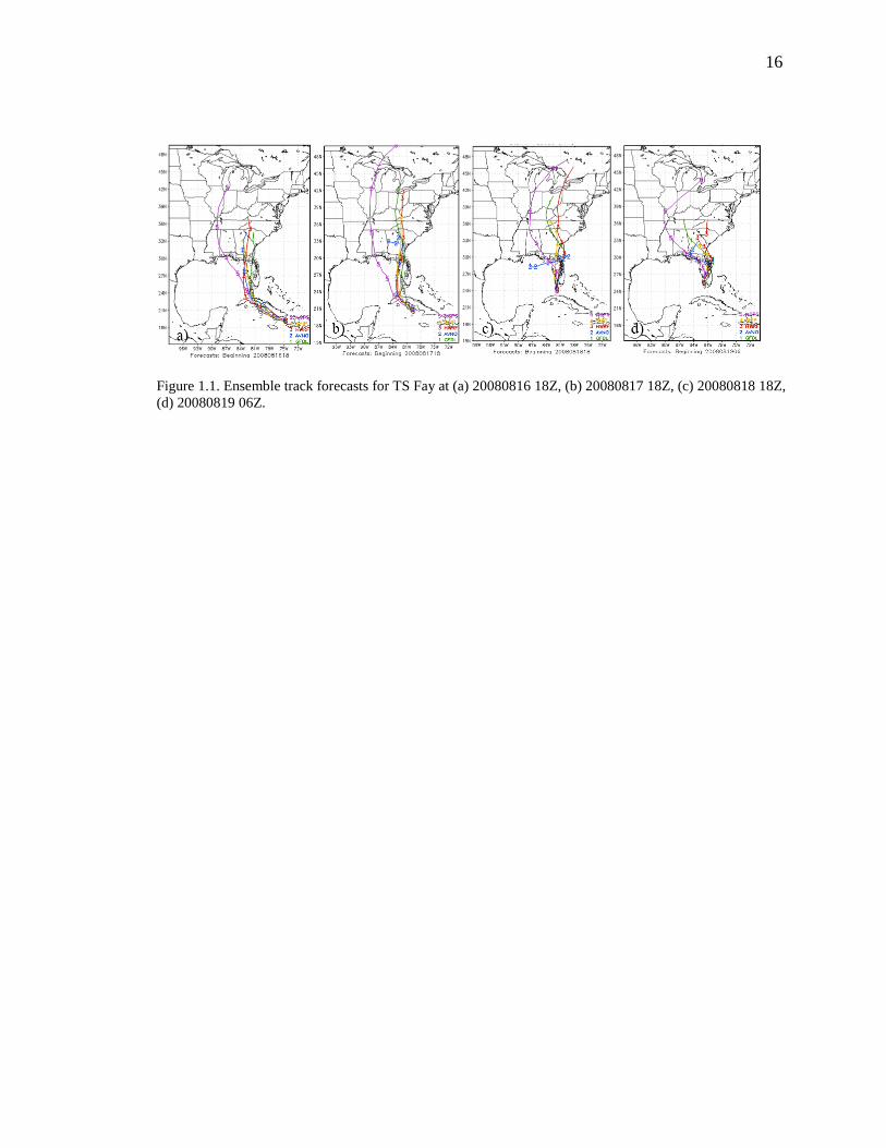
interactions. Evidence of this can be seen in Figure 1.1, where the hurricane modeling

ensemble attempts to predict TS Fay‟s (2008) track and landfall position at various hours

out from Fay‟s observed landfall at 20080819 09z. In addition, a particularly difficult

case to forecast was TC Erin (2007) that did not form the typical TC eye feature until

over land and by hindsight physical evidence of the continuance of tropical properties

was later discovered as incorrectly classified overland by NWS forecasters (Monteverdi

and Edwards 2010).

11

11

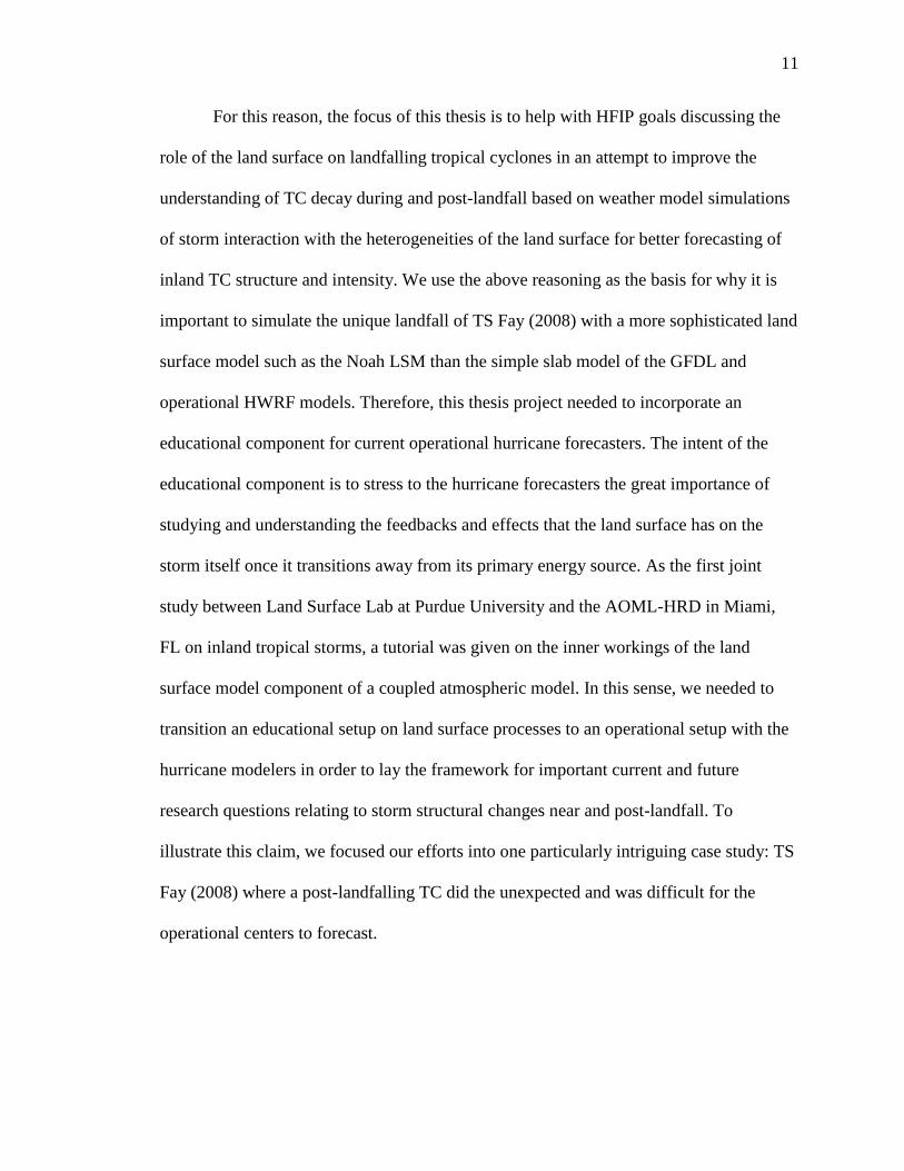
For this reason, the focus of this thesis is to help with HFIP goals discussing the

role of the land surface on landfalling tropical cyclones in an attempt to improve the

understanding of TC decay during and post-landfall based on weather model simulations

of storm interaction with the heterogeneities of the land surface for better forecasting of

inland TC structure and intensity. We use the above reasoning as the basis for why it is

important to simulate the unique landfall of TS Fay (2008) with a more sophisticated land

surface model such as the Noah LSM than the simple slab model of the GFDL and

operational HWRF models. Therefore, this thesis project needed to incorporate an

educational component for current operational hurricane forecasters. The intent of the

educational component is to stress to the hurricane forecasters the great importance of

studying and understanding the feedbacks and effects that the land surface has on the

storm itself once it transitions away from its primary energy source. As the first joint

study between Land Surface Lab at Purdue University and the AOML-HRD in Miami,

FL on inland tropical storms, a tutorial was given on the inner workings of the land

surface model component of a coupled atmospheric model. In this sense, we needed to

transition an educational setup on land surface processes to an operational setup with the

hurricane modelers in order to lay the framework for important current and future

research questions relating to storm structural changes near and post-landfall. To

illustrate this claim, we focused our efforts into one particularly intriguing case study: TS

Fay (2008) where a post-landfalling TC did the unexpected and was difficult for the

operational centers to forecast.

12

12

References

Arndt, D. S., J. B. Basara, R. A. McPherson, B. G. Illston, G. D. McManus, and D. B.

Demko, 2009: Observations of the overland reintensification of Tropical Storm

Erin (2007). Bull. Amer. Meteor. Soc., 90, 1079–1093.

Bao, S., R. Yablonsky, D. Stark, L. Bernardet, 2010: HWRF User‟s Guide. The

Developmental Testbed Center, Boulder, CO, 88pp.

Bassill, N. P., and M. C. Morgan, 2006: The overland reintensification of Tropical Storm

Danny (1997). Preprints, 27th Conf. on Hurricanes and Tropical Meteorology,

Monterey, CA, Amer. Meteor. Soc., 6A.6.

Bosart, L. F., and G. M. Lackmann, 1995: Postlandfall Tropical Cyclone

Reintensification in a Weakly Baroclinic Environment: A Case Study of

Hurricane David (September 1979). Mon. Wea. Rev., 123, 3268-3291.

----------------, and J. A. Bartlo, 1991: Tropical storm formation in a baroclinic

environment. Mon. Wea. Rev., 119, 1979–2013.

Chang, H., D. Niyogi, A. Kumar, C. Kishtawal, J. Dudhia, F. Chen, U.C. Mohanty, M.

Sheperd, 2009: Possible relation between land surface feedback and the post-

landfall structure of monsoon depression. Geophys. Res. Lett., 36 (L15826),1-6.

13

13

Chen, F. and Coauthors, 2006: Description of the Characteristics of the NCAR High-

Resolution Land Data Assimilation System. J. Appl. Meteorol. Climatol., 46, 694-

713.

Ek M. B., K. E. Mitchell, Y. Lin, E. Rodgers, P. Grunmann, V. Koren, G. Gayno, and J.

D. Tarpley, 2003: Implementation of the Noah land surface model advances in the

NCEP operational mesoscale Eta model. J. Geophys. Res., 108(D22), doi:

10.1029/2002JD003296.

Emanuel, K. A., J. Callaghan, and P. Otto, 2008: A hypothesis for the re-development of

warm-core cyclones over northern Australia. Mon. Wea. Rev., 136, 3863–3872.

Evans, J. L. and R. E. Hart, 2003: Objective indicators for the life cycle evolution of

extratropical transition for Atlantic tropical cyclones. Mon. Wea. Rev., 131, 909-

925.

Gopalakrishnan, S. G., F. Marks, L. Qingfu, T. Marchok, D. Sheinin, N. Surgi, R. Tuleya,

R. Yablonsky, and X. Zhang, 2010: Hurricane Weather Research and Forecasting

(HWRF) model Scientific Documentation. L. Bernardet, Ed., 75.

----------------------------, F. Marks, X. Zhang, J.-W. Bao, K.-S. Yeh, and R. Atlas, 2011:

The experimental HWRF system: a study on the influence of horizontal resolution

on the structure and intensity changes in tropical cyclones using an idealized

framework. Mon. Wea. Rev., 139, 1762-1784.

Kehoe, J., S. Raman, and R. Boyles, 2010: Characteristics of Landfalling Tropical

Cyclones in North Carolina. Marine Geodesy, 33(4), 394-411.

14

14

Knupp, K. R., J. Walters, and M. Biggerstaff, 2005: Doppler profiler and radar

observations of boundary layer variability during the landfall of Tropical Storm

Gabrielle. J. Atmos. Sci., 63, 234-251.

Kurihara, Y., R. E. Tuleya, and M. Bender, 1998: The GFDL hurricane prediction system

and its performance in the 1995 hurricane season. Mon. Wea. Rev., 126, 1306-

1322.

Laing, A., and J. L. Evans, 2010: Introduction to Tropical Meteorology, A

Comprehensive Online and Print Textbook. 2nd ed. University Corporation for

Atmospheric Research, [Available online at

http://www.meted.ucar.edu/tropical/textbook]

Liu, Q., N. Surgi, S. Lord, W. S. Wu, D. Parrish, S. Gopalakrishnan, J. Waldrop, and J.

Gamache, 2006: Hurricane Initialization in HWRF Model Extended Abstract,

27th Conf. on Hurricanes and Tropical Meteorology, Monterey, CA, Amer.

Meteor. Soc., 8A.2 [Available online at

http://ams.confex.com/ams/27Hurricanes/techprogram/paper_108496.htm]

Monteverdi, J. P., and R. Edwards, 2008: Documentation of the overland reintensification

of Tropical Storm Erin over Oklahoma, August 18, 2007. Preprints, 24th Conf. on

Severe Local Storms, Savannah, GA, Amer. Meteor. Soc., P4.6.

-------------------------------------------, 2010: The redevelopment of a warm core structure

in Erin: A case of inland tropical storm formation. Electron. J. Severe Storms

Meteorol., 5(6), 1-18.

Noilhan, J. and S. Planton, 1988: A simple parameterization of land surface processes for

meteorological models. Mon. Wea. Rev., 117, 536-549.

15

15

Rhome, J. R., and S. Raman, 2006: environmental influences on tropical cyclone

structure and intensity: A review of past and present literature. Indian J. of

Marine Sci., 35(2), 61-74.

Singh R., P. K. Pal, C. M. Kishtawal, and P. C. Joshi, 2005: Impact of bogus vortex for

track and intensity prediction of tropical cyclone. J. Earth Syst. Sci., 114, 427-436.

Tuleya, R. E., and Y. Kurihara, 1978: A numerical simulation of the landfall of tropical

cyclones. J. Atmos. Sci., 35, 242–257.

-----------------, M. A. Bender, and Y. Kurihara, 1984: A simulation study of the landfall

of tropical cyclones using a movable nested-mesh model. Mon. Wea. Rev., 112,

124–136.

-----------------, 1994: Tropical storm development and decay: Sensitivity to surface

boundary conditions. Mon. Wea. Rev., 122, 291–304.

-----------------, 2010: Test results using the NOAH LSM in the operational HWRF

system. Recorded Presentation, 29th Conference on Hurricanes and Tropical

Meteorology, Tucson, AZ, Amer. Meteor. Soc., 12C.7 [Available online at

http://ams.confex.com/ams/29Hurricanes/techprogram/paper_168976.htm]

16

16

Figure 1.1. Ensemble track forecasts for TS Fay at (a) 20080816 18Z, (b) 20080817 18Z, (c) 20080818 18Z,

(d) 20080819 06Z.

17

17

CHAPTER 2 TS FAY 2008 CASE STUDY1

2.1 Introduction

Tropical systems weaken and decay rapidly after making landfall. This decay has

been attributed to multiple factors such as change in surface characteristics, latent heat

flux source, as well as changes in shear (Tuleya 1994, Kimball 2004). The occurrence of

TC strengthening post-landfall is therefore an anomalous feature and is of

hydrometeorologic interest to the forecast and disaster response community. Only a few

cases of overland storm reintensification have been observed for the Atlantic tropical

storms in recent years including TCs Erin (2007), Danny (1997), Fran (1996) and David

(1979). Unique to our case study, Tropical Storm Fay (2008) became organized through a

first-time intensification overland as opposed to a reintensification as previously

mentioned with other notable systems. Interestingly, Fay did not develop a typical TC

eye-like structure until after landfall over South Florida (Stuart and Beven 2009). Also of

interest is Fay‟s overland intensification and best track proximity to Lake Okeechobee

and the Everglades which leads to the motivation to study whether the unique Florida

surface features may have provided a surface feedback to aid with Fay‟s intensification

overland.

1 Chapter 2 of this thesis is adapted to fit the Purdue University thesis format and its content in its entirety

is taken from the recent publication cited here: Bozeman, M. L., D. Niyogi, S. Gopalakrishnan, F. Marks Jr.,

X. Zhang, and V. Tallapragada, 2011: An HWRF-based ensemble assessment of possible land surface

feedbacks on the post-landfall intensification of Tropical Storm Fay of 2008. Natural Hazards. doi:

10.1007/s11069-011-9841-5.

18

18

National Hurricane Center (NHC) best track reports that TS Fay made landfall at Cape

Romano, Florida at 0845 UTC August 19. Later that day, Fay was observed at its peak

intensity of 60 knot maximum winds and a central sea level pressure of 986 mb at 1800

UTC, which occurred near Lake Okeechobee. The eye feature that developed post-

landfall was visible in the Melbourne (KMLB) radar imagery from 0929 UTC August 19

until 0212 UTC August 20 (Figure 2.1). Fay moved steadily over South Florida and

crossed into the Atlantic Ocean at approximately 0600 UTC on August 20, 2008.

Therefore, it is hypothesized that the surface features such as the occurrence of the lake,

and the local landuse heterogeneity may have contributed to the brief but significant

overland intensification of TS Fay. We report on the analysis of the changes in TC

structure over land using the NHC best track, observations, and Hurricane WRF

modeling system (Gopalakrishnan et al. 2010). The HWRF simulations of Fay were

conducted from August 19, 2008 00Z until August 21 00Z, with particular focus on the

period where the storm center was over the land surface (between August 19 09Z and 20th

06Z).

Studies have shown that the underlying surface characteristics such as terrain,

land use, soil temperature and moisture, albedo and surface roughness have great

influence on convective systems that pass over areas with surface heterogeneities (e.g.,

Pielke 2001). In the case of landfalling hurricanes, these systems need to seek energy

from the available inland moisture and energy fluxes instead of the ocean, as they

continue to dissipate. Due to the shape of Florida‟s coastline, a number of studies have

examined the role of the frequent land and sea breezes on Florida‟s weather (e.g. Pielke

1974, Wilson and Megenhardt 1997, Baker et al. 2001). Numerical simulations of Florida

19

19

sea breeze circulation have also shown that due to its large area and circular shape, Lake

Okeechobee also causes its own lake breeze circulation (Baker et al. 2001). This lake

breeze affects both the weather near the lake causing a cloud free zone above the lake

waters during the day, and affects the intensity and duration of the nearby sea breeze

circulation occurring on Florida‟s eastern coastline (Pielke 1974, Boybeyi and Raman

1992).

The overall objective of this study is to understand the impact of the land surface

feedbacks on the inland intensification of TS Fay using the HWRF modeling system. The

specific goals of our experiments are to: (1) study the effects of different land surface

parameterization schemes on the HWRF forecast, (2) study the effect of land surface

features (and heterogeneity) including Lake Okeechobee and the Everglades, through

idealized simulations. Additionally, (3) assess the relative impact of different ensemble

experiments on the model forecast and delineate feedbacks that may have contributed to

the post-landfall intensification of tropical storm Fay in HWRF simulations.

2.2 Numerical Model and Experiments

Model runs were conducted using the HWRF model that implements a stationary

parent domain (27 km) and moving inner nest (9 km), and is initialized with the 30-

second geography resolution using the WRF Pre-processing System (WPS). This

configuration of the WRF Non-hydrostatic Mesoscale Model (NMM) core is based on the

operational configuration of the NOAA modeling and research centers, in which the

different physics options used have been specifically tested for hurricane forecasting and

are preferred for predicting TC structure and dynamics (Gopalakrishnan et al. 2010). A

20

20

detailed description of the HWRF model configurations for our experiments is listed in

Table 2.1; and an in depth explanation of the HWRF model domain on a rotated latitude-

longitude E-staggered grid are reported in Gopalakrishnan et al. 2011. Since our focus is

on TCs over land, the model was initialized only 9 hours before landfall and as a result

we do not use the Princeton Ocean Model (POM) or NCEP coupler components of the

operational HWRF. This also helps reduce the degrees of freedom when evaluating Fay‟s

land-atmosphere interactions as opposed to variable sea surface temperatures. In addition,

the data needed to initialize the loop current in the POM were unavailable for this case.

All simulations are compared to the NHC best track products to assess accuracy in

intensity forecasts, and to each other to determine forecast differences between the

various alterations of the HWRF model configuration and forecast environment. All

results presented in this paper are analyzed from the inner moving nest since it

implements a higher model horizontal resolution of 9 kilometers.

Experiments were designed to test the HWRF forecast using two different LSMs:

the GFDL slab model and the Noah land surface model. The GFDL slab model from

Tuleya (1994) uses a bulk subsurface layer to prognostically predict the ground surface

temperature assuming the following surface energy balance:

aLse

vaLep

L

RTRVLCWETLE

TVCcH

GFSLEHT

4

From these energy balance equations, G represents the net ground surface heat flux, H,

the surface sensible heat flux, LE is the surface evaporative heat flux, 4

LT is the

emission from the Earth‟s surface and finally, FS is the net downward radiative

21

21

surface flux. The drag coefficient Ce is calculated from the Monin-Obukhov methods

referenced in Tuleya (1974), where V is the low-level wind speed, va is the virtual

potential temperature of the surface air. WET represents the wetness coefficient, Rs and Ra

are the mixing ratios of the saturated surface land temperature and of the low-level air, L

is the latent heat of condensation, ρ is the density of the low-level air, while cp is the

specific heat of air. Once assuming this surface energy balance Tuleya, following

Deardorff (1978) predicts the slab model ground surface temperature with the formula

below:

21

/

:

4

ss

ss

LL

cd

where

dc

FSLEHT

t

T

In the slab surface temperature equation, ρscs is the soil heat capacity, d is the damping

depth where λ is the thermal conductivity of the soil and τ is the period of forcing (24

hours). Since the only predicted variable in the slab model is the surface temperature, all

surface fluxes (enthalpy and momentum) are calculated by the surface layer scheme, the

surface wetness remains constant with time and is initially specified by the input GFS

lateral boundary conditions. During the development of the GFDL hurricane model, the

GFDL slab model with conjunction of the GFDL radiation scheme met the requirements

for realistic TC activity over land at the time (Gopalakrishnan et al. 2010).

Gopalakrishnan et al. (2010) tests with HWRF highlight that the simple GFDL slab

model sufficiently replicates important features such as the cold pool land temperature

beneath a TC. The simulation of the cold pool is important over land to greatly reduce the

22

22

surface evaporation and aid rapid TC decay. We hypothesize however, that the Noah

model (Ek et al. 2003) will produce more realistic forecasts due to its implementation of

four soil layers and explicit prediction of surface soil temperature, moisture, runoff,

sensible heat flux, evaporation, and snow cover. Noah also includes a more complex

vegetation representation through use of the USGS 1992 and MODIS 2001 land use

datasets. In this study, the Slab model runs are the control because current operational

hurricane models (i.e., GFDL hurricane model and HWRF) employ the GFDL Slab

model as the default LSM, while numerous operational NCEP models use the Noah LSM,

which we will use as the experimental LSM.

To study the impact of the unique Florida surface features, the USGS landuse, and

soil type (top and bottom soil type) of the 30 second resolution geography tiles were

altered to reflect the “removal” of Lake Okeechobee and the Everglades in experimental

runs (locations of these features are indicated in Figure 2.2). Landuse and soil type

categories were changed to values similar to each feature‟s surroundings per the default

USGS 1992 dataset (Figure 2.2) to avoid creating artificial heterogeneous land and soil

surfaces. Removal of Lake Okeechobee/Everglades is reflected by changing the 24

category USGS landuse category, 16 category soil type - top and bottom from

water/wooded wetland to dry cropland and pasture/grassland, sand/sand, and

sand/bedrock respectfully. The model land/sea mask is then calculated by the model and

is determined from the landuse category as either water or land. Changes were done to

the soil and landuse to dry out the land surface which the TC will pass over to investigate

the impacts on the surface environment and TC rainfall distribution and structure. The

relative influence of each surface feature is evaluated by a variable isolation analysis

23

23

through model experiments (Table 2.2). Experiments were conducted with both Lake

Okeechobee and the Everglades removed (NOWET), and additional model runs to

separately test the contribution of (a) only Lake Okeechobee removed (NOLAKE) and (b)

only the Everglades removed (NOGLADES), to determine the relative impact of each

wet area on the moisture and temperature distribution of tropical storm Fay.

Sections 3 and 4 of this paper discuss the results of the model simulations and

conclusions, respectfully. The organization of the sub-sections of section 3 is as follows:

a description of the results from the control and default LSMs is in section 3.1,

simulations specific to Lake Okeechobee and the Everglades in section 3.2, and an

assessment of the improved results seen with the use of the Noah LSM, a Noah-based

HWRF ensemble is analyzed in section 3.3. In sections 3.4 and 3.5,we revisit the Noah

LSM intensity analysis and then proceed to take a more in-depth analysis of possible

influences of storm decay. The storm decay discussion involves simulations

implementing real-world (ie default) geography, all-ocean over the region of Florida, and

finally no ocean surrounding Florida while Lake Okeechobee and the Everglades are still

present in the idealized geography from the WRF Preprocessing System (WPS). In

section 3.5, a simplistic water budget is analyzed from the model simulations used in

section 3.4. Since forecast skill is largely assessed based on forecast track, each

subsequent section of the results and discussion begin with an analysis of the forecast

track error, referred to here as FTE. In TC prediction, FTE is defined as the great circle

distance of the forecast latitude (latF) and longitude (lonF) points from the observed best

track latitude (latB) and longitude (lonB) points over the globe. This is calculated from

Powell and Aberson (2001):

24

24

Next, TC intensity forecasts are of importance to assess the internal storm dynamics and

also to investigate the causes of periods of storm strengthening and weakening. These

results are discussed in the 3b sections. Section 3.1b analyzes the intensity forecasts for

simulations using the GFDL Slab and Noah LSM. Section 3.2b analyzes the model

intensity forecasts focused on the effects of the presence of Lake Okeechobee and the

Everglades and uses results of the no ocean simulation to supplement the discussion

(3.2d), while 3.3b investigates intensity forecasts from the findings in the Noah-based

ensemble. Subsequent 3c sections involve investigation of the model simulated rainfall

accumulations.

2.3 Results and Discussion

2.3.1 Influence of GFDL Slab versus Noah LSM

a. Forecast Track Errors

Figure 2.3a shows the six hour FTE (km) between model runs using the GFDL

Slab and Noah LSM against the best track. Our focus is on the track error columns

corresponding to “S” and “N” at this time. Both Slab and Noah deviate from the best

track over the ocean from the initial time, but in the first six hours, Noah and Slab have a

similar forecast track, and then begin to separate from each other after this time. The

Noah run begins to realign itself by intersecting the best track near the time of the

observed landfall at Cape Romano, while Slab places the landfall location further west.

Overall, the Noah run stays fairly consistent to the best track forecast, but with a slight

lonFlonBlatFlatBlatFlatBFTE cos*cos*cossin*sinarccos*11.111

25

25

six hour position lag resulting in a lower sum of six hour forecast errors (sum FTE) of

78.39 km. The Slab model keeps the storm following Florida‟s western coastline and

farther into northern Florida resulting in a very large total FTE of 401.37 km.

b. Intensity Errors

Figure 2.4a shows the maximum sustained winds along the forecast track for Slab

versus Noah. From the time series, both Slab and Noah correctly categorize Fay‟s TS

intensity; however both LSM runs underestimate the observed peak winds of 60 knots at

18Z on August 19. Once over land, Slab shows a dramatic reduction in wind speed

especially from 18Z August 19 until 03Z August 20. Noah was able to correctly predict

the secondary peak winds of 55 knots at 12Z August 19 and 00Z August 20, but these

winds weakened quickly after 00Z, and thus under predicting the 50 kt observation at

06Z August 20. Figure 2.5a shows the along track minimum sea level pressure (MSLP)

over time for Slab versus Noah. From the initial time, both LSMs drop the central

pressure drastically for the brief period over the ocean, then show slow storm filling after

landfall. Both Slab and Noah keep the central pressure of Fay too deep during the time of

the observed minimum pressure of 986 mb, and instead simulate 984.8 mb and 983.6 mb,

respectively. The runs only show a moderate weakening of Fay after 18Z August 19,

while Slab shows a secondary strengthening starting at 22Z on August 19.

2.3.2 Influence of Lake Okeechobee and Florida Everglades

a. Forecast Track Error

Figure 2.3b shows results for the six hour FTE for the Slab and Noah simulations

involving land surface feature changes of the presence or lack of Lake Okeechobee and

26

26

the Everglades. We focus on the track error table of both columns of “NW”, “NL”, and

“NG” corresponding to “SLAB” and “NOAH”. Every land change model run follows

their parent LSM run well; however, the tracks of the land changes for the Slab model

have more variance between each six hour position. Slab shows six hour position

variation from forecast hours 12 to 30; whereas the Noah runs show position variation

from the parent LSM for forecast hours 24 to 30. Interestingly, the different land changes

for the Slab model have lower total FTEs than the Slab run itself. The land changes with

Noah have lower total FTEs with the exception of the NL run, which has a higher total

FTE from Noah by 0.71 km. The lowest FTEs for all Noah runs occurred at forecast

hours 18 to 24, while FTE for all Slab runs steadily increased over time as the storm was

incorrectly moving westward.

b. Intensity Error

Figures 2.4b and 2.5b show time series of the along track maximum sustained

winds and MSLP for the land change runs with the Noah LSM only. These time series

are only for the Noah runs since the Noah track brought the storm closer to the surface

features being studied. Figure 2.4b shows that the runs follow the original Noah wind

time series fairly closely over time, and continue to classify Fay with TS strength. All

wind curves agree over water, but after landfall, the curves begin to deviate slightly from

each other. A similar pattern to the storm maximum winds can be seen in the 10 meter

sustained winds over time (not shown). On average, the Noah run maintains the highest

winds and usually is the upper bounding curve while the NW run is the lower bound in

this time series. As Fay nears Florida‟s eastern coastline, the wind speeds of the NL and

NW runs increase and have a higher magnitude than the Noah and NG runs beginning at

27

27

02Z August 20th. Differences between the wind speeds at 06Z August 20 are small, 1 to

1.5 knot differences. Figure 2.6 shows the spatial plots of the wind differences. In any run

where the lake is removed reveals a large under prediction of the 10 m wind by as much

as 10 to 30 knots. In cases where the Everglades are taken out, the differences are

typically +/- 5 knots, with the location of the differences varying from run to run. Figure

2.5b shows that the land changes do have a small influence on the TC central pressure.

Shortly after landfall, the MSLP curves deviate from each other, with the largest pressure

differences after the observed peak intensity. The NL and NW runs predict Fay to

weaken faster after passing the peak time, as the Noah and NG runs show a slow steady

weakening until 06Z August 20. These plots indicate that the presence of Lake

Okeechobee caused slight but detectable enhancement of the storm central pressure and

wind speed as the TC crosses near and over the lake; the contribution of the possible lake

feedback will be discussed in the next section.

A cross sectional analysis (see Figures 2.7 and 2.8) was completed to view

additional differences in surface variables along land and directly above the lake at the

time of Fay‟s peak intensity. The cross section was taken at constant latitude of 26.95° N

across Florida and Lake Okeechobee with longitude varying from -82.1° W to -80.1° W.

The cross section lines in the Slab runs are shifted slightly due to the variation in forecast

track between land change runs that were more pronounced in Slab simulations. The

cross section analysis reveals that for both Noah and Slab, when the lake is present there

are increased surface latent heat fluxes and 10 m wind speeds directly over the lake. This

is consistent with the increased humidity and decreased roughness of the water surface.

Both the LSMs predict a lower central pressure than observed by the best track, yet Slab

28

28

has a weaker central pressure than Noah by about 1 mb. Consistent with the intensity

analysis, runs without Lake Okeechobee have a weaker central pressure, though the SG

curve follows the SL and SW curves as opposed to being similar to the Slab parent run. A

study by Sousounis and Fritsch (1994) shows that lakes may enhance precipitation in

strong synoptic systems, but will not alter storm tracks. Their study conducted for the

Great Lakes, suggests that lakes may help storms intensify and cause a 3-4 mb drop in

MSLP for strong synoptic extratropical cyclones passing over the lake region. Shen et al.

(2002) studied the simulated rate of decay on landfalling TCs using the GFDL hurricane

model when standing surface water of various depths was present over the land surface.

They concluded that a half meter of standing surface water was able to reduce the rate of

TC decay after landfall. In our model study though, the pressure is not lowered to the

same degree as the effect of the Great Lakes on extratropical systems.

c. Surface Heterogeneity effects on Rainfall Accumulations

The simulation of TC rainfall magnitude and spatial coverage was also dependent

on choice of the land surface scheme, in part due to the forecast track. Figure 2.9 shows

the differences in rainfall accumulation from the default LSM runs for the land surface

changes described in Table 2.3. In particular, the spatial coverage of the rainfall maxima

covers a broader area in the Noah run, while the Slab based maxima is placed farther

north with a greater magnitude by 100 mm. Overall, the TC rainband circulation is more

coherent in the difference plots than with the Slab LSM. In all runs, there is an expected

eastward precipitation bias which is consistent with observations that the maximum rain

fall occurs within the right-front quadrant of the system as it moves forward in time

(Marchok et al. 2007). The most impact to the rain field can be seen with each NW run,

29

29

and is mainly due to elimination of Lake Okeechobee. There are small but noticeable

differences between rain accumulations when the lake is not present resulting in an under

prediction of nearly 20 to 30 mm for most runs, and up to 40 to 60 mm in the case of NW

and SW runs. For this case, the Everglades have a minimal impact on rainfall

accumulation though its elimination did affect the magnitude by over predicting rainfall

near the Everglades and the Florida Keys in the Slab LSM runs. Interestingly, the

presence of the lake also prevents an over prediction of rainfall directly of the south east

coast of Florida shown in the NG run. As seen in Figure 2.9, the land surface physics

choice and land surface heterogeneity causes detectable impacts on the TC rainfall

distribution.

d. TC development solely influenced by land surface moisture sources

To further isolate the possible influence of Lake Okeechobee and the Florida

Everglades on Fay, the ensemble runs were compared to a simulation with both the Gulf

of Mexico and the Atlantic Ocean moisture sources removed (NOOCEAN). In this

simulation, the removal of these ocean basins are reflected by changing the 24 category

USGS landuse category, 16 category soil type top and bottom from water to cropland and

woodland mosaic, sand, and sand respectfully, while the original values of the lake and

everglades remained unchanged. The goal of this model run is to eliminate the TC spiral

rainbands from obtaining moisture from the ocean basins as the storm center is

influenced by land. Instead, this forces Fay to take in moisture from the only available

sources - Lake Okeechobee and the Florida Everglades. We hope that including this

simulation will isolate and further help to reveal the influence specifically from these

features.

30

30

Figure 2.10 shows the forecast track of the NOOCEAN run compared to the NHC

best track (left) and the default Noah track (right). NOOCEAN tracks similarly to the best

track and the default Noah from the initialization time through forecast hour 12, then the

track brings Fay westward from the best track through the middle of the Florida peninsula

however not as far west as the Slab run. This forecast track results in a total FTE of 647

km error. A time series of the NOOCEAN maximum winds and MSLP (not shown)

reveals a TC of a much weaker intensity with a peak wind of 51.7 kt at 12Z Aug 19

followed by a steady decrease in wind speed. For the MSLP, there is an initial drastic

drop in pressure to 984.2 mb followed by a rapid filling of the central pressure up to

1001.14 mb at 06Z on Aug 20th

.

Now that they are not being overpowered by the influence of the ocean water,

Figures 2.10 and 2.11 help to describe the specific contributions of the Florida surface

features to the TC structure. Referring back to Figure 2.10, the rainfall has accumulated

in a diagonal swath across Florida and encompassing Lake Okeechobee. The difference

plot of the accumulated rainfall (Figure 2.10) shows that the total rain field has been

reduced since the NOOCEAN simulation is a weaker storm in a drier environment, yet

has a grossly overpredicted rain swath as compared to the default Noah run probably due

to the fact that the Everglades and Lake Okeechobee were the only sources of moisture.

Perhaps the moist surface features allowed for enhanced precipitation in the region near

Lake Okeechobee that could possibly lead to a surface feedback between the falling

precipitation and the accumulating soil moisture over a larger area. This feedback follows

the study of Emmanuel et al. (2008) for the warm-core cyclone rainfall in Northern

Australia and Chang et al. 2009 for the Indian monsoon region. In Figure 2.11, the

31

31

difference in the 10 m wind reveals that since the lake is a water body with low

roughness length, the NOOCEAN wind field is highest surrounding the lake which

agrees with Kimball (2004). The high winds over the lake found in the NOOCEAN run

may also suggest that in the model simulation, Lake Okeechobee does create its own

circulation (Boybeyi and Raman 1992).

2.3.3 Noah Ensemble Runs

To further analyze the improvements in the storm simulation using the Noah LSM,

we conducted a Noah-based model ensemble assessment with changes to the PBL

parameterization, and the initial conditions (Table 2.3).

a. Forecast Track Errors

Referring to Figure 2.3c for the six hour forecast track error between ensemble

model runs using the Noah LSM for simulations involving changes to the land surface

features, PBL parameterization, and model initial conditions. Interestingly, all of the new

ensemble members have higher total FTEs than Noah and the land change runs of which,

both the initial condition runs have the highest track error. The N6B run has a large FTE

of 296.91 km as it moved the storm too quickly through Florida for all hours except

during the first six hours into the forecast. Also the N6B run puts Fay at the Atlantic coast

at 00Z August 20 and then alters the track northward and into the Atlantic before 06Z

August 20, no other run exhibits this behavior. Despite having fewer hours of error to

sum up, the N6A run also has a large FTE of 213.53 km since the track stops short as the

storm weakens never reaching the Florida‟s eastern coastline. The NY and NM runs also

end their tracks in the middle of Florida as well, but do not have nearly as large error as

32

32

the N6A run. These systems that dissipate over Florida would have a large intensity error

which is discussed later. With exception of the NY run at 06Z August 19, the PBL

change runs have a lower six hourly track error than Noah and all the land change runs

for 06Z August 19 until 18Z August 19, with the least error at 18Z. Thus the effect of the

land surface feedbacks affecting the TCs is through the boundary layer forcing.

b. Intensity Error

Figures 2.4c and 2.5c show time series of the along track maximum sustained

winds and MSLP for the Noah LSM ensemble. In contrast to the Noah land changes,

each new member wind field (Figure 2.4c) varies dramatically from each other from the

initial time until the end of the period of interest and are not able to match the best track

winds for any forecast hour. On average, the N6B run maintains the highest winds and

usually is the upper bounding curve while the N6A run is the lower bound in the time

series. The N6B run does not match the best track wind observation at 00Z Aug 19 since

this model was initialized six hours prior and has already deviated from the best track

winds. This is not the case for most of the other members, which were initialized at 00Z

and therefore correspond to the best track at this time. Even though the N6A run was

initialized at 06Z Aug 19, it under predicts the maximum winds to 51.1 kt instead of

matching the best track value of 55 kt winds. While all other members are unable to

predict a TC with the correct wind intensity at 18Z Aug 19, the N6B run actually predicts

a much stronger TC with peak winds of 66.1 kt, a weak category 1 hurricane. Both the

changed PBL runs (MYJ and YSU) start out with strong winds over ocean, then reduce

the wind speed post-landfall, and still miss the observed peak wind at 18Z. For most

33

33

forecast times, the NY run has stronger winds than the NM until 00Z Aug 20 when the

NY weakens the winds quickly while the NM curve begins to flatten out through 06Z

Aug 20. From this time series one can see that the only members that match the best track

winds most consistently are the default HWRF configuration with Noah, and Noah land

change runs each implementing the GFS PBL scheme and initialized at 00Z Aug 19.

Figure 2.5c shows that changes in the PBL scheme and initial conditions also

have a dominant effect on Fay‟s along track MSLP over time for all the Noah ensemble

members. Again, the N6B and N6A runs are the outer bounds for the stronger and weaker

central pressure intensity respectively. Changing the PBL parameterization resulted in

weaker TCs. The Noah and land change runs simulate a stronger central pressure at the

time of peak intensity, while the PBL changes result in a weaker central pressure for all

hours after landfall as compared to the land change runs. This finding is consistent with

Gopalakrishnan et al. (2010) who also found that HWRF runs with the MYJ PBL and

surface layer parameterization schemes caused weaker TCs. On average, the NY member

is the closest to accurately predicting Fay‟s central pressure. Despite predicting a slightly

weaker central pressure during the peak time, NY displays the weakening after 18Z to a

more realistic degree than any other ensemble member. NM however, weakens the TC

too quickly after the time of peak intensity, while the land changes cause little variability

and continue to maintain the TC strength as it nears Florida‟s eastern coast.

c. PBL and Initial Condition effects on Rainfall Accumulations

The effect of changes in the model physics and initial conditions on the TC

intensity forecast additionally alters the TC rainfall accumulations (Figure 2.12). As

expected, due to the N6A model producing an extremely weak TC, the rain shield is also

34

34

severely weakened in both breadth of spatial coverage and rainfall intensity as compared

to all other ensemble members. Alternatively, producing a TC of hurricane status, N6B

develops a rain shield with broad coverage over Florida and a western rainfall bias as

opposed to all other members which have an eastern accumulation bias. N6B also causes

the TC to accumulate precipitation with a higher intensity over a larger area, specifically

over Southern Florida and the Everglades and centrally over a wide area around Lake

Okeechobee. NY and NM simulate a rain shield of moderate coverage when compared to

the original Noah and N6B runs, probably due to the weaker intensity forecasts. In

addition, NM accumulations consistently follow slightly to the east of the forecast storm

track for the entire period. This feature in the NM rainfall pattern is also displayed in

plots of the rainfall rates and rate differences between the Noah ensemble members (not

shown). The NY rain also follows this pattern in the rainfall rates, yet is not pronounced

in the NY rainfall accumulations. Of note, are the peak rainfall accumulations in the N6B

and NM members that show accumulations between 400-500mm directly to the west, and

between 300-400mm to the north east of Lake Okeechobee. In addition, the rain rate

differences of the ensemble members (not shown) reveals that the NY (NM) over (under)

predicts areas of rainfall by 20 to 40 mm directly to the north and south of Lake

Okeechobee. Thus the impacts of the initial conditions and PBL scheme choice provides

an equally strong influence on the rain field as the choice of land surface

parameterization scheme.

35

35

2.3.4 Revisiting the Noah LSM Intensity Analysis and Mechanisms for Decay

Since the Slab LSM was unable to produce an adequate track forecast, a

generalized analysis of TS Fay decay mechanisms will only include model simulations

using the Noah LSM. Figure 2.13 shows different parameters for decay of the Noah

default simulation versus the Noah-based ALLOCEAN and NOOCEAN idealized

simulations. By including non-landfall simulations with ALLOCEAN and NOOCEAN,

we can investigate the role of oceanic sustenance of the TC if Florida were not present,

and the rapid decay of the TC from being initialized and traversing over a non-moist

region for an extended period of time (in addition to the roughness and friction

characteristics of the land surface). In addition, the storm structure due to the transition of

the TC from water to land can be compared in the default Noah run compared to the non-

landfalling simulations.

The predicted storm tracks of the ocean test simulations (not shown) have Fay

tracking similarly to the best track and Noah default in the ALLOCEAN run and more to

the west (similar to the Slab track) with the NOOCEAN run (NOOCEAN track is seen

and discussed earlier in Figure 2.10). Figure 2.13a shows the simulated MSLPs compared

the six hour best track MSLP. The default Noah simulation is the most comparable to the

best track, while the ALLOCEAN and NOOCEAN are the upper and lower bounds on

the central pressure respectively. These results agree with past studies of landfalling TCs

which are not able to maintain strength over land. Figure 2.13b shows the maximum

sustained winds at 10 m compared to the NHC best track storm sustained winds. The 10

m Vmax is displayed since it takes into account the local exposure to the surface

roughness from the land surface model. However, the maximum sustained winds in the

36

36

storm (ie “storm Vmax”), (not shown for ALLOCEAN and NOOCEAN, while the Noah

default Vmax is seen in Figure 2.4a) are more comparable to the NHC Vmax since they

do not address the local roughness and are better representative of open terrain exposure.

As such, the values of the 10 m Vmax is are lower and probably more in agreement with

local station observations which were not studied in this paper. In Figure 2.13b,

NOOCEAN shows a rapid decay of winds while ALLOCEAN reveals extremely strong

winds despite being restricted to the 10 m level. In a simplistic view, these two plots

indicate that TCs intercepting and/or traversing overland does in fact drastically reduce

storm strength when compared to an all water case.

TC decay post landfall is attributed to numerous factors based on land surface

characteristics, yet the greatest of these is the reduction of latent heat energy and

evaporation once over land (Tuleya and Kurihara 1978). Surface latent and sensible heat

fluxes, frictional stresses, and roughness are important variables for TC maintenance over

land and therefore are reviewed to see how the predicted TC intensity may have been

affected by these parameters (Tuleya and Kurihara 1978, Dastoor and Krishnamurti 1991,

Shen et al. 2002). Figures 2.13c through 2.13e show the storm tangential latent heat flux,

sensible heat flux, and frictional stress (with zero value fluxes removed) to help assess

factors contributing in the rates of strengthening and decay observed in these simulations.

For the latent heat flux field (Figure 2.13c), the Noah default curve is as expected with

higher latent heat over ocean and then a significant reduction in latent heat similar to the

NOOCEAN curve post landfall. Since Lake Okeechobee is still present in the

NOOCEAN case, it is interesting to find that this latent heat curve shows a slight increase

between 12Z and 18Z on Aug 19th

when the TC track nears the lake. After the slight

37

37

increase in the latent heat flux, the NOOCEAN tangential flux tapers off near the end of

the timeseries, and never returns back to the low initial latent heat values as in the

beginning of the forecast period before the lake moisture source was introduced. The

ALLOCEAN latent heat curve however, shows a more dramatic flux increase near 18Z.

Since latent heat performs as expected when the system transitions from ocean to

land, it is possible that the sensible heat flux may play a more dominant role in

maintenance or decay in the case of TS Fay. Figure 2.13d shows the sensible heat flux for

each of the ocean test cases and again the ALLOCEAN and NOOCEAN are the upper

and lower bounds of the flux over time. While one would think that the Noah default case

should act similarly to the NOOCEAN case overland, we must highlight that the Florida

peninsula is a landmass with a small width compared to the scale of the storm. So as TS

Fay passes over the Florida landscape, it is still being influenced by the surrounding sea.

As the storm crosses over the Florida peninsula, the rainbands swirling over the ocean are

still impacting the energy transfer within the core by either slowing the amount of

evaporation or through advection of moisture inwards. Evidence of this can be seen by

the fact that the Noah default sensible heat does not drop down as far as the NOOCEAN

sensible heat curve despite being over land. Horizontal flux gradients between the

peninsula land and surrounding sea are smeared by the horizontal advection as the storm

rainbands swirl over both land and sea.

Tangential frictional stress over time (Figure 2.13e) suggests that for a water case,

as in ALLOCEAN, the stronger the wind, the stronger the frictional stress becomes over

time. However for a land case the evolution of the frictional stress is more complicated.

As seen in NOOCEAN, there is an initial increase in stress yet as the wind spins down

38

38

due to interactions with the land surface, the net stress decreases more rapidly in model

simulations over land. Further evidence of both of these trends can be seen in the Noah

default curve for frictional stress, where just after landfall there is a brief peak in stress

similar to the NOOCEAN case. Then once the Noah default storm nears Lake

Okeechobee, another peak in stress develops (similar to the ALLOCEAN case) since the

wind field may have become stronger from traversing over a water body with less surface

roughness (Shen et al. 2002).

2.3.5 Noah LSM Water Budget

So far, study results have presented changes to what the land surface is

experiencing due to land experiments and the evolution of variables affecting TC

intensity. This section however, examines a simulated water budget and in doing so

changes the study focus from the local land scale to storm scale, specifically near the TC

eye and eyewall within a radius of 270 km. A simple water budget for Fay is investigated

to learn more about how the moisture is being used inside the TC and its distribution

inside the system. In addition, budget terms are separated into radial and vertical

components in an attempt to isolate possible moisture contributions from the storm

circulation and land surface respectfully. While numerous studies were fortunate enough

to observe the wind fields and develop momentum, heat and moisture budgets for specific

TC cases (eg. Gamache et al. 1993; Marks and Houze 1987; McBride 1981) and model

simulations for TCs (eg. Kurihara and Tuleya 1981; Estoque 1962) the studies of

Gamache et al. (1993) and Marks and Houze (1987) resulted in a schematic of a

hurricane water budget (see Figure 1 from Gamache et al. 1993, Figures 9a,b and 10 from

39

39

Marks and Houze 1987) while Braun (2006) presents a more recent review of past

observed and simulated water budget studies.

Similar to Gamache et al. (1993), this water budget calculates budget terms over a

cylindrical volume taken within 270 km from the center of the TC. The model output is

transformed to cylindrical polar height coordinate system following Gopalakrishnan et al.

(2011), refer to section 2c from this study for more details on the HWRF cylindrical

transformation. Budget terms used in this analysis are adapted from the moisture flux

convergence (hereafter, MFC) formulas from Banacos and Schultz (2005) who

researched the use of MFC as a diagnostic forecast tool to locate regions favorable for

convective initiation in the mid-latitudes (MFC was also incorporated into the Kuo

cumulus parameterization for the tropics, Kuo 1965,1974). Once the conservation of

water vapor is expanded by the mass continuity equation and written in flux form for

cylindrical coordinates, an analysis of the advection and convergence components of the

horizontal and vertical MFC terms in the local tendency of water vapor equation is

presented for TS Fay.

zw

r

V

ru

tdt

d rr

(1)

qwz

qVt

q

dt

dqh

(2)

where:

r

VuVj

ri r

rh ,,ˆˆ

40

40

Horizontal Advection Term (A)

q

r

V

r

qu r

Horizontal Convergence Term

(C)

rV

r

uq r

Vertical Divergence Term (D) qwz

Vertical Moisture Flux (F)

qw

z1000

Within the local tendency of water vapor equation (2), terms A and C arise from the

vector identity of the second term on the RHS multiplied by negative one (also known as

MFC), while term D (also known as the negative vertical MFC) is the third term on the

RHS of the equation. The vertical moisture in term D is investigating only the moisture

that is entering the storm system as opposed to the moisture being precipitated out of the

system. Generally with TC systems more moisture is being precipitated out of the system

than entering the system (or study volume) so term D is considered a moisture

“divergence.” In the water budget analysis plots (Figures 2.14 and 2.15), a 6-hourly

azimuthally averaged radius-height cross section for only the radial terms of terms A, C

and terms D and F for the model vertical levels from 35 m to 15 km is used to represent

the moisture distribution in conjunction with the secondary wind circulation in the TC.

Results are from model simulations ALLOCEAN (NAO), Default (N) and NOOCEAN

(NNO) presented at forecast hour 18, corresponding to 18Z Aug 19 which was the

observed peak intensity of TS Fay.

41

41

All panels in Figure 2.14 show the secondary wind circulation (uw vector field)

characteristic to a TC. When comparing between simulations however, NOOCEAN has

the weakest inflow and upper outflow compared to the other simulations obviously due to

its weaker intensity as seen earlier in Figure 2.13a,b. The moisture convergence panels

(left column) each show a strongly saturated inflow layer with varying depths according

to storm intensity. Notice the sloping of the moist inflow region in the ALLOCEAN and

default plots. Due to the extreme amounts of moist inflow all other regions of the TC

seem dry in comparison. However, warm color regions in the convergence panels are

actually indicating regions of intense updrafts where moisture is being rapidly moved

away from the moisture source (inflow) and seen as divergence in the figure. These

updraft regions are co-located with regions of strong vertical gradients of the vertical

moisture divergence (contours), the combination of these terms represent the eyewall

convection. Again, the strength of the convection (shaded) and vertical gradients

(contours) vary with TC intensity at 18Z Aug 19. Since Lake Okeechobee is present in

both the Noah default and NOOCEAN simulations, it is possible that its presence is

revealed in the panels by the second peak in vertical divergence contours in the default

image and the secondary peak in convection in the shaded region slightly farther away

from the TC center in the NOOCEAN image. The moisture advection panels in Figure

2.14 (right column) show both how the moist inflow advection varies in intensity by the

simulated storm intensity and the expansion of the moist region in the mid-levels from

the eyewall throughout the mid-troposphere. The NOOCEAN simulation is unable to

distribute its moisture to the mid-troposphere due to its weak intensity, however the

contours of the vertical moisture in the default run seem weaker than the ALLOCEAN

42

42

run since the default has already approached its peak state (Figures 2.4a and 2.5a) and is

now at a weakened steady state while ALLOCEAN continues to intensify with time

(Figures 2.13a,b). The lake moisture signature is harder to see in the radial advection

panels since these images represent the horizontal advection of moisture throughout the

storm as opposed to moisture being supplied vertically to the system from the surface.

Therefore, the radial components are not drivers of the system but help to locate regions

of convection and moisture distribution within the TC. Kuo (1974) also claimed that in

TC cases the tropical cumulus convection would depend mostly on the large-scale

vertically integrated MFC.

Figure 2.15 describes the horizontal gradient of the vertical moisture flux located

at the PBL top (2000 m) and 70 m above the surface. Note the large differences in

magnitude of the vertical flux between the different levels in the atmosphere; at 2000 m

there are much larger values than at 70 m. The gradients of the moisture flux between

ALLOCEAN and Noah default look quite similar except that the default run has a larger

spatial extent of moisture flux at both levels. This feature is probably due to the presence

of Lake Okeechobee. At the lower level, the region of positive moisture flux is bounded

by regions of negative moisture flux which could be indicative of the lake being bounded

by agricultural regions which are much drier in contrast to the lake. The moisture

signature of Lake Okeechobee is most clearly seen in the NOOCEAN simulation since it

is one of the only sources of moisture; this signature is especially evident at the 2000 m

level. From these results, it is conceivable to conclude that even the horizontal gradients

of the vertical moisture flux assist in the sustenance of the traversing TC overland. In

addition, the small gradients at the near-surface grow larger further up in the atmosphere

43

43

by PBL processes as seen in the magnitude differences between the vertical levels. This

conclusion agrees with statements from Banacos and Shultz (2005) that in some

situations, the horizontal variations of the vertical moisture may be more important than

the advective terms.

2.4 Conclusions

The findings of this study related to HWRF model simulations of TS Fay (2008),

summarizes that three features contribute to changes in TC NWP forecasts. First, that

land surface parameterization is of importance to the storm forecast track but did not

significantly impact the intensity. The improved track resulted in rainfall distributions

that correctly reflect observations from hurricane studies that the core of heavy TC rain is

predominantly in the narrow swath closest to the storm center (Lonfat 2004, Marchok et

al. 2007, and Rodgers et al. 2009). In this sense, the Noah LSM seems to have better

forecast performance over the GFDL Slab model. Secondly, initial boundary conditions

and PBL scheme are shown to be vital to TC development and intensity forecasts of

maximum winds and central pressure over land. Lastly, surface heterogeneity reflected in

the land change simulations played a small but detectable role in forecast alterations. It

can be seen that the presence of a lake does in fact cause a drop in central pressure of a

storm, but not enough to be a major contributor to TC intensity prediction or rainfall

distribution in real world situations where an ocean basin is present.

Thus specific to the TS Fay case, the intensification overland may have been a as

result of a small scale anomaly due to land surface heterogeneity and confluence caused

by benevolent boundary conditions. Essentially, at the time of peak intensity, all factors

44

44

acted together to produce this chance occurrence of intensification despite the known fact

that TCs decay rapidly overland. The possible effects from the presence of the Florida

Everglades was not important for Fay; mostly due to the storm track north of the

Everglades. This track did not provide a substantial feedback despite the larger spatial

coverage of the Everglades over Lake Okeechobee. In addition, Florida‟s geography may

also have allowed for the ocean to continually influence the energy transport in the core

of the system despite the central pressure tracking over land. Evidence of this comes from

the fact that the tangential sensible heat flux curve in the Noah default member did not

decrease significantly towards the extremely dry environment in the NOOCEAN case. As

the latent heat flux produced expected results after landfall, in the TS Fay case perhaps

the sensible heat flux was dominant in enabling the storm to strengthen over land as

opposed to being greatly influenced by the inland moisture sources. From the water

budget analysis, it was shown that the vertical moisture terms were more important for

maintenance of Fay in the idealized simulations than the radial terms. Radial terms were

essentially used to identify regions of moisture and convection, yet were not drivers for

the storm. The fact that the vertical moisture terms from the budget seemed more

important further agrees with the earlier finding that the fluxes are most important for

sustenance of the TC. In the model framework, the combined effects of the land surface

physics and initial conditions created a boundary layer feedback which seemed beneficial

for the chance of Fay‟s intensification. The importance of this land surface feedback

through the boundary layer is emphasized by the severe TC weakening resulting from the

use of the two different boundary layer (YSU and MYJ) parameterizations.

45

45

A secondary result of these experiments revealed that the HWRF model is

sensitive to land surface and PBL physics. In addition, we also found that it is important

to have the correct initial conditions for the land surface and PBL to interact together and

produce a forecast simulation that is closer to observed events. If the GFDL Slab LSM

had produced a comparable track, we would have further investigated its differences from

the Noah and completed a Slab water budget to see how moisture was treated using this

other LSM. To further test this HWRF sensitivity, we plan to conduct this analysis on a

case with longer inland track (e.g. TS Erin 2007) and a large dataset of landfalling storms

in order to see if model findings from the current study are transferable to multiple

HWRF forecasts of storms of varying intensities. Thus, our limitation in the current study

is that it focuses on a single case and the findings from the land cover change simulations

are probably not transferable. Again, we will be investigating the predictive performance

of the GFDL Slab versus the Noah LSM and testing additional physics options for

supplementary analysis as needed to assist in improving the HWRF model. This larger

study will include an in-depth analysis and verification of the precipitation intensity and

distribution as well as a more advanced analysis of storm intensity forecasts overland.

46

46

References

Baker, R. D., B. H. Lynn, A. Boone, W. Tao, J. Simpson, 2001: The influence of soil

moisture, coastline curvature, and land-breeze circulations on sea-breeze-initiated

precipitation. J. Hydrometeor., 2, 193-211.

Boybeyi, Z., and S. Raman, 1992: A three-dimensional numerical sensitivity study of

convection over the Florida peninsula. Bound.-Layer Meteorol., 60, 325-359.

Braun, S. A. 2006: High-resolution simulation of Hurricane Bonnie (1998). Part II: Water

budget. J. Atmos. Sci., 63, 43-64.

Chang, H., D. Niyogi, A. Kumar, C. Kishtawal, J. Dudhia, F. Chen, U.C. Mohanty, M.

Sheperd 2009: Possible relation between land surface feedback and the post-

landfall structure of monsoon depression. Geophys. Res. Lett., 36(L15826), 1-6.

Dastoor, A., and T. N. Krishnamurti, 1991: The landfall and structure of a tropical

cyclone: the sensitivity of model predictions to soil moisture parameterizations.

Bound.-Layer Meteorol., 55, 345-380.

Deardorff, J. W. 1978: Efficient prediction of ground surface temperature and moisture,

with inclusion of a layer of vegetation. J. Geophys. Res., 83, 1889-1903.

47

47

Chen, F. and Coauthors, 2006: Description of the Characteristics of the NCAR High-

Resolution Land Data Assimilation System. J. Appl. Meteor. Climatol., 46, 694-

713.

Ek, M. B., K. E. Mitchell, Y. Lin, E. Rodgers, P. Grunmann, V. Koren, G. Gayno, and J.

D. Tarpley, 2003: Implementation of the Noah land surface model advances in the

NCEP operational mesoscale Eta model. J. Geophys. Res., 108(D22), doi:

10.1029/2002JD003296.

Emmanuel, K. A., J. Callaghan, and P. Otto, 2008: A hypothesis for the redevelopment of

warm-core cyclones over northern Australia. Mon. Wea. Rev., 136, 3863-3872.

Estoque, M. A., 1962: Vertical and radial motions in a tropical cyclone. Tellus, 14(4),

394-400.

Ferrier B.S., 2005: An efficient mixed-phase cloud and precipitation scheme for use in

operational NWP models. Eos., Trans. Amer. Geophys. Union, 86 (Spring

Meeting Suppl.), Abstract A42A-02.

Gamache, J. F., R. A. Houze Jr., and F. D. Marks Jr., 1993: Dual-aircraft investigation of

the inner core of Hurricane Norbert. Part III: Water budget. J. Atmos. Sci., 50(19),

3221-3243.

Gopalakrishnan, S. G., F .Marks, L. Qingfu, T. Marchok, D. Sheinin, N. Surgi, R. Tuleya,

R. Yablonsky, and X. Zhang, 2010: Hurricane Weather Research and Forecasting

(HWRF) model Scientific Documentation. L. Bernardet, Ed., 75.

48

48

----------------------------, X. Zhang, J. Bao, K. Yeh and R. Atlas 2011: The experimental

HWRF system: A study on the influence of horizontal resolution on the structure

and intensity changes in tropical cyclones using an idealized framework. Mon.

Wea. Rev., 139, 1762-1784.

Hong, S.-Y., and H.-L. Pan, 1996: Nonlocal boundary layer vertical diffusion in a

medium-range forecast model. Mon. Wea. Rev., 124, 2322-2339.

---------------, and H.-L. Pan, 1998: Convective trigger function for a mass-flux cumulus

parameterization scheme. Mon. Wea. Rev., 129, 1164-1178.

Kimball, S., 2004: A modeling study of the sensitivity of landfalling hurricanes to surface

evaporation and surface roughness. Extended Abstracts, 26th

Conference on

Hurricanes and Tropical Meteorology, Miami, FL, Amer. Meteor. Soc. 12D.6.

[Available online at http://ams.confex.com/ams/pdfpapers/75662.pdf.]

Kuo, H. L., 1965: On formation and intensification of tropical cyclones through latent

heat release by cumulus convection. J. Atmos. Sci., 22, 40-63.

-------------, 1974: Further studies of the parameterization of the influence of cumulus

convection on large-scale flow. J. Atmos. Sci., 31, 1232-1240.

Kurihara, Y., and R. E. Tuleya, 1981: A numerical simulation study on the genesis of a

tropical storm. Mon. Wea. Rev., 109, 1629-1653.

Lacis, A. A., and Hansen J. E., 1974: A parameterization for the absorption of solar

radiation in the earth‟s atmosphere. J. Atmos. Sci., 31, 118–133.

Lonfat, M., F. D. Marks, and S. Chen, 2004: Precipitation distribution in tropical

cyclones using the Tropical Rainfall Measuring Mission (TRMM) Microwave

Imager: A global perspective. Mon. Wea. Rev., 132, 1645-1660.

49

49

Marchok, T., R. Rogers, and R. Tuleya, 2007: Validation schemes for tropical cyclone

quantitative precipitation forecasts: evaluation of operational models for U.S.

landfalling cases. Wea. Forecasting, 22, 726-746.

Marks, F. D., Jr., and R. A. Houze Jr., 1987: Inner core structure of Hurricane Alicia

from airborne Doppler radar observations. J. Atmos. Sci., 44(9), 1296-1317.

McBride, J. L., 1981: Observational analysis of tropical cyclone formation. Part III:

Budget analysis. J. Atmos. Sci., 38, 1152-1166.

Moon, I., I. Ginis, T. Hara, and B. Thomas, 2007: Physics-based parameterization of air-

sea momentum flux at high wind speeds and its impact on hurricane intensity

predictions. Mon. Wea. Rev., 135, 2869-2878.

Pielke, R., 1974: A three-dimensional numerical model of the sea breezes over south

Florida. Mon. Wea. Rev., 102, 115-139.

------------, 2001: Influence of the spatial distribution of vegetation and soils on the

prediction of cumulus convective rainfall. Rev. Geophys., 39, 151–177.

Powell, M. D., and S. D. Aberson 2001: Accuracy of the United States tropical cyclone

landfall forecasts in the Atlantic basin (1976-2000). Bull. Amer. Meteorol. Soc.,

82, 2749-2767.

Rodgers, R., F. Marks, and T. Marchok, 2009: Tropical cyclone rainfall. Encyclopedia of

Hydrological Sciences, John Wiley and Sons, pp.1-22. doi:

10.1002/0470848944.hsa030.

Schwarzkopf, M D., and S. Fels, 1991: The simplified exchange method revisited: An

accurate, rapid method for computation of infrared cooling rates and fluxes. J.

Geophys. Res., 96, 9075-9096.

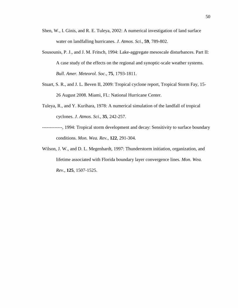
50

50

Shen, W., I. Ginis, and R. E. Tuleya, 2002: A numerical investigation of land surface

water on landfalling hurricanes. J. Atmos. Sci., 59, 789-802.

Sousounis, P. J., and J. M. Fritsch, 1994: Lake-aggregate mesoscale disturbances. Part II:

A case study of the effects on the regional and synoptic-scale weather systems.

Bull. Amer. Meteorol. Soc., 75, 1793-1811.

Stuart, S. R., and J. L. Beven II, 2009: Tropical cyclone report, Tropical Storm Fay, 15-

26 August 2008. Miami, FL: National Hurricane Center.

Tuleya, R., and Y. Kurihara, 1978: A numerical simulation of the landfall of tropical

cyclones. J. Atmos. Sci., 35, 242-257.

-------------, 1994: Tropical storm development and decay: Sensitivity to surface boundary

conditions. Mon. Wea. Rev., 122, 291-304.

Wilson, J. W., and D. L. Megenhardt, 1997: Thunderstorm initiation, organization, and

lifetime associated with Florida boundary layer convergence lines. Mon. Wea.

Rev., 125, 1507-1525.

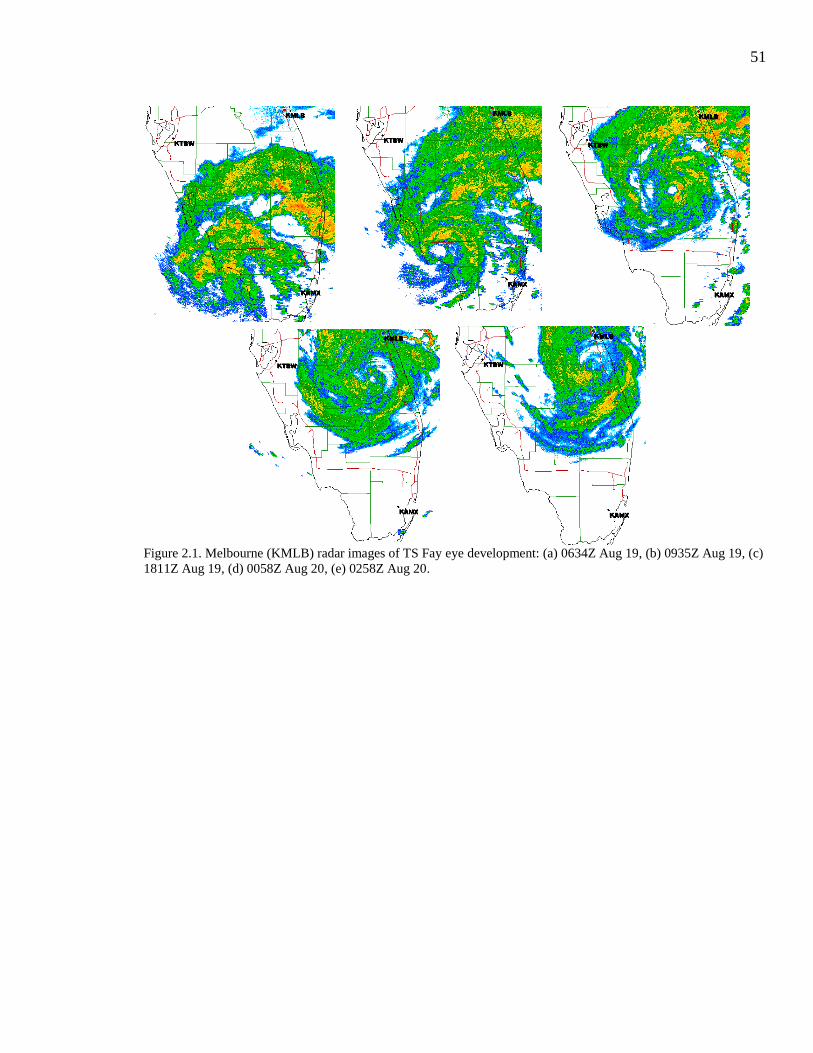
51

51

Figure 2.1. Melbourne (KMLB) radar images of TS Fay eye development: (a) 0634Z Aug 19, (b) 0935Z Aug 19, (c)

1811Z Aug 19, (d) 0058Z Aug 20, (e) 0258Z Aug 20.

52

52

Table 2.1. HWRF model configuration for experiments.

Domains

Horizontal 27km (80° x 80°) Stationary

9km (6° x 6°) Moving Nest

(Gopalakrishnan et al. 2010b)

Vertical 42 vertical levels with model top at 50 mb

Lateral Boundary Conditions 6-hr GFS forecast on 1° grid

WPS Geography Resolution 30 second resolution

Model Physics

Number of Soil Layers 4

Microphysics Etamp_hwrf scheme (Ferrier 2005)

Long-wave Radiation Modified GFDL scheme

(Schwarzkopf and Fels 1991)

Short-wave Radiation Modified GFDL scheme

(Lacis and Hansen 1974)

Surface-layer GFDL surface-layer scheme

(Moon et al. 2007)

Land-surface GFDL Slab LSM (default) / Noah LSM

(Tuleya 1994, Deardorff 1978) / (Ek et al. 2003)

Planetary Boundary Layer NCEP GFS Scheme

(Hong and Pan 1996)

Cumulus scheme Simplified Arakawa-Schubert scheme

(Hong and Pan 1998)

53

53

Table 2.2. LSM model runs with changed surface features.

Run Name LSM Used Experimental Change

Slab (S) GFDL Slab

LSM

NOWET (SW) GFDL Slab

LSM

Lake and Everglades

removed NOLAKE (SL) GFDL Slab

LSM

Lake Okeechobee removed

only NOGLADES

(SG)

GFDL Slab

LSM

Everglades removed only

Noah (N) Noah LSM

NOWET (NW) Noah LSM Lake and Everglades

removed NOLAKE (NL) Noah LSM Lake Okeechobee removed

only NOGLADES

(NG)

Noah LSM Everglades removed only

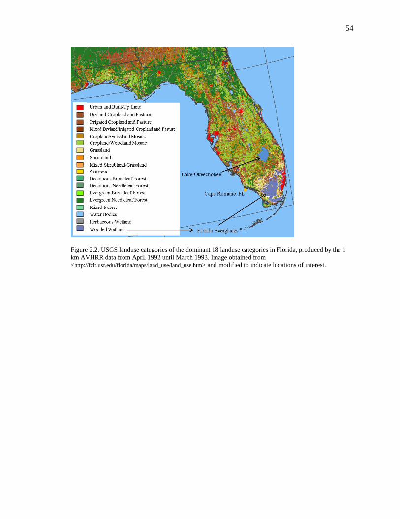
54

54

Figure 2.2. USGS landuse categories of the dominant 18 landuse categories in Florida, produced by the 1

km AVHRR data from April 1992 until March 1993. Image obtained from

<http://fcit.usf.edu/florida/maps/land_use/land_use.htm> and modified to indicate locations of interest.

55

55

Table 2.3. Noah LSM ensemble members.

Member Name LSM Used Experimental Change

Noah (N) Noah LSM

NOWET (NW) Noah LSM Lake and Everglades removed

NOLAKE (NL) Noah LSM Lake Okeechobee removed only

NOGLADES

(NG)

Noah LSM Everglades removed only

YSU PBL (NY) Noah LSM YSU PBL Scheme

MYJ PBL (NM) Noah LSM MYJ PBL Scheme

6 Before (N6B) Noah LSM Model Start Time: 2008-08-18 18 Z

6 After (N6A) Noah LSM Model Start Time: 2008-08-19 06 Z

56

56

GFDL SLAB LSM NOAH LSM

Time fcst

hr S SW SL SG N NW NL NG NY NM N6B N6A

08/18

18Z -6 0

08/19

00Z 0 0 0 0 0 0 0 0 0 0 0 25.09

08/19

06Z 6 14.80 15.46 14.91 15.42 15.24 15.50 15.33 15.40 18.77 13.92 23.26 0

08/19

12Z 12 19.68 18.92 19.23 19.19 14.79 14.40 14.20 14.95 12.46 5.32 12.39 45.35

08/19

18Z 18 28.11 29.92 28.32 28.65 11.96 13.59 12.47 12.85 4.05 9.92 49.25 27.28

08/20

00Z 24 147.56 140.46 143.34 141.81 6.37 10.83 11.41 5.19 21.53 33.08 75.29 44.58

08/20

06Z 30 191.24 187.58 187.32 192.33 30.03 22.02 25.68 25.66 44.87 62.52 111.63 96.32

Sum FTE 401.37 392.35 393.12 397.40 78.39 76.34 79.10 74.05 101.68 124.77 296.91 213.53

Figure 2.3. HWRF model forecast track errors (FTE): (a) GFDL Slab versus Noah, (b) GFDL Slab land changes (SW,

SL, SG) versus Noah LSM land changes (NW, NL, NG), (c) Noah LSM ensemble members (NW, NL, NG, NY, NM,

N6B, N6A). Fay best track (BT) forecast is indicated with the thick black line.

BT

S

N

(a)

S,SW,SL,SG

N,NW,NL,NG

BT

(b)

N,NW,NL,NG

N6B

NY NM

N6A

BT

(c)

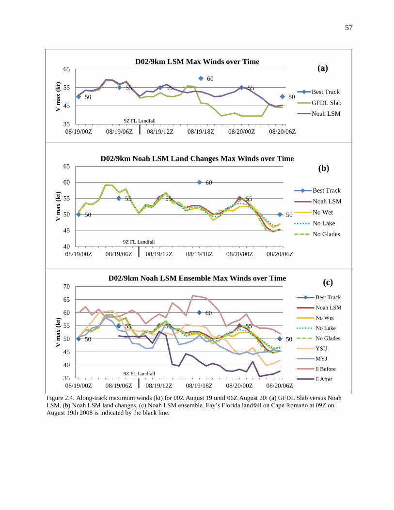
57

57

Figure 2.4. Along-track maximum winds (kt) for 00Z August 19 until 06Z August 20: (a) GFDL Slab versus Noah

LSM, (b) Noah LSM land changes, (c) Noah LSM ensemble. Fay‟s Florida landfall on Cape Romano at 09Z on

August 19th 2008 is indicated by the black line.

50

55 55

60

55

50

35

45

55

65

08/19/00Z 08/19/06Z 08/19/12Z 08/19/18Z 08/20/00Z 08/20/06Z

V m

ax (

kt)

D02/9km LSM Max Winds over Time

Best Track

GFDL Slab

Noah LSM

(a)

9Z FL Landfall

50

55 55

60

55

50

40

45

50

55

60

65

08/19/00Z 08/19/06Z 08/19/12Z 08/19/18Z 08/20/00Z 08/20/06Z

V m

ax (

kt)

D02/9km Noah LSM Land Changes Max Winds over Time

Best Track

Noah LSM

No Wet

No Lake

No Glades

(b)

9Z FL Landfall

50

55 55

60

55

50

35

40

45

50

55

60

65

70

08/19/00Z 08/19/06Z 08/19/12Z 08/19/18Z 08/20/00Z 08/20/06Z

V m

ax (

kt)

D02/9km Noah LSM Ensemble Max Winds over Time

Best Track

Noah LSM

No Wet

No Lake

No Glades

YSU

MYJ

6 Before

6 After

(c)

9Z FL Landfall

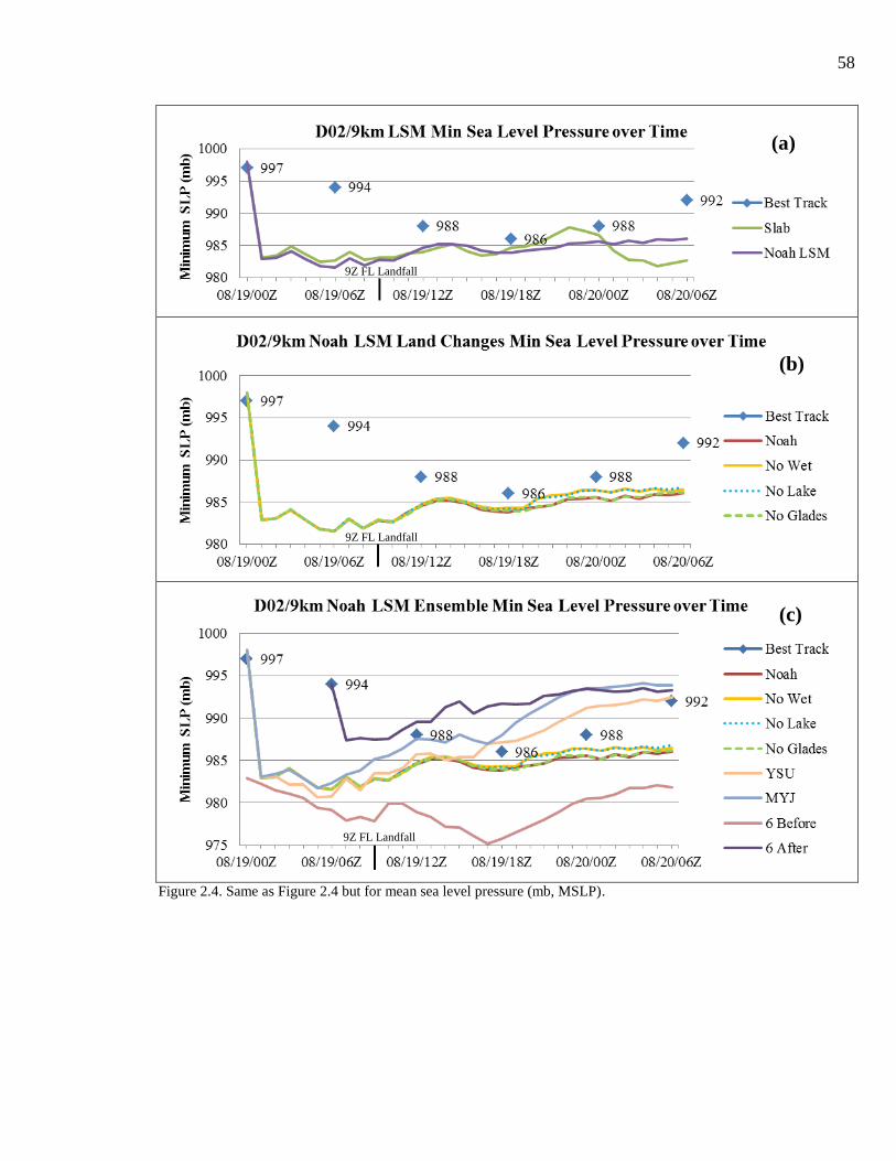
58

58

Figure 2.4. Same as Figure 2.4 but for mean sea level pressure (mb, MSLP).

(a)

(b)

(c)

9Z FL Landfall

9Z FL Landfall

9Z FL Landfall

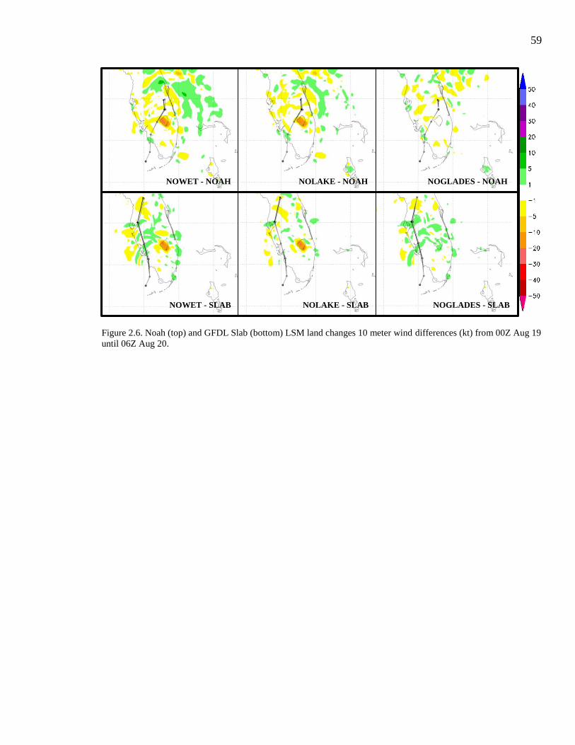
59

59

Figure 2.6. Noah (top) and GFDL Slab (bottom) LSM land changes 10 meter wind differences (kt) from 00Z Aug 19

until 06Z Aug 20.

NOWET - NOAH NOLAKE - NOAH NOGLADES - NOAH

NOGLADES - SLAB NOLAKE - SLAB NOWET - SLAB

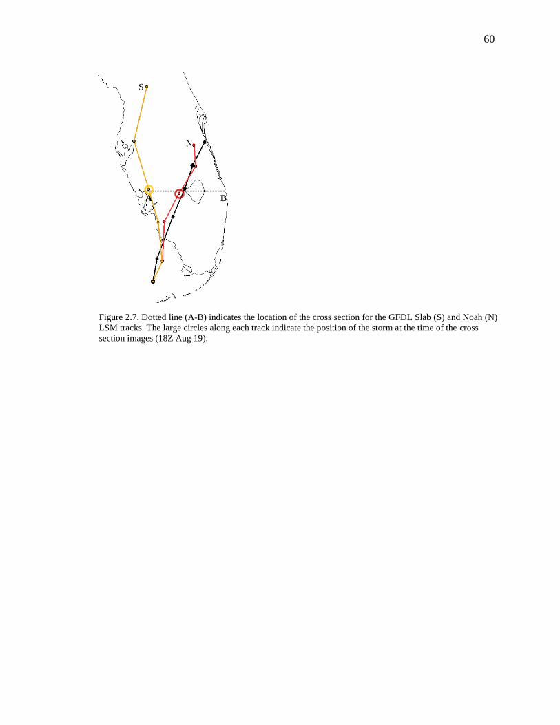
60

60

Figure 2.7. Dotted line (A-B) indicates the location of the cross section for the GFDL Slab (S) and Noah (N)

LSM tracks. The large circles along each track indicate the position of the storm at the time of the cross

section images (18Z Aug 19).

S

N

A B

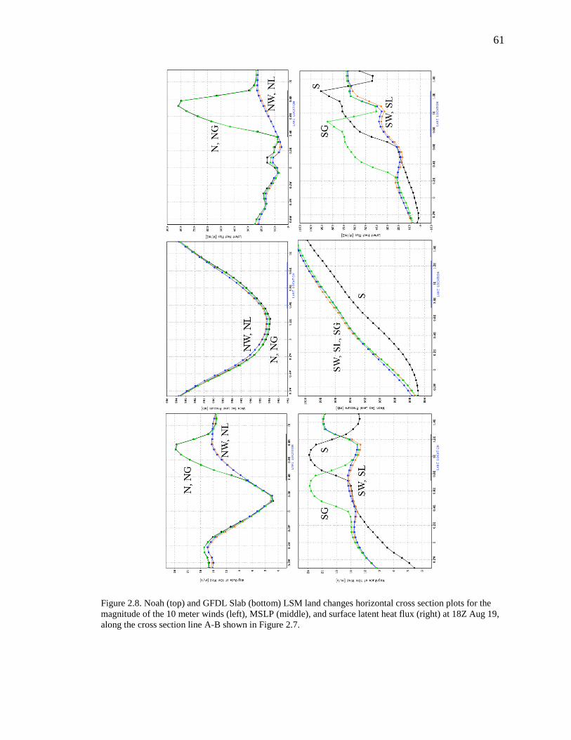
61

61

Figure 2.8. Noah (top) and GFDL Slab (bottom) LSM land changes horizontal cross section plots for the

magnitude of the 10 meter winds (left), MSLP (middle), and surface latent heat flux (right) at 18Z Aug 19,

along the cross section line A-B shown in Figure 2.7.

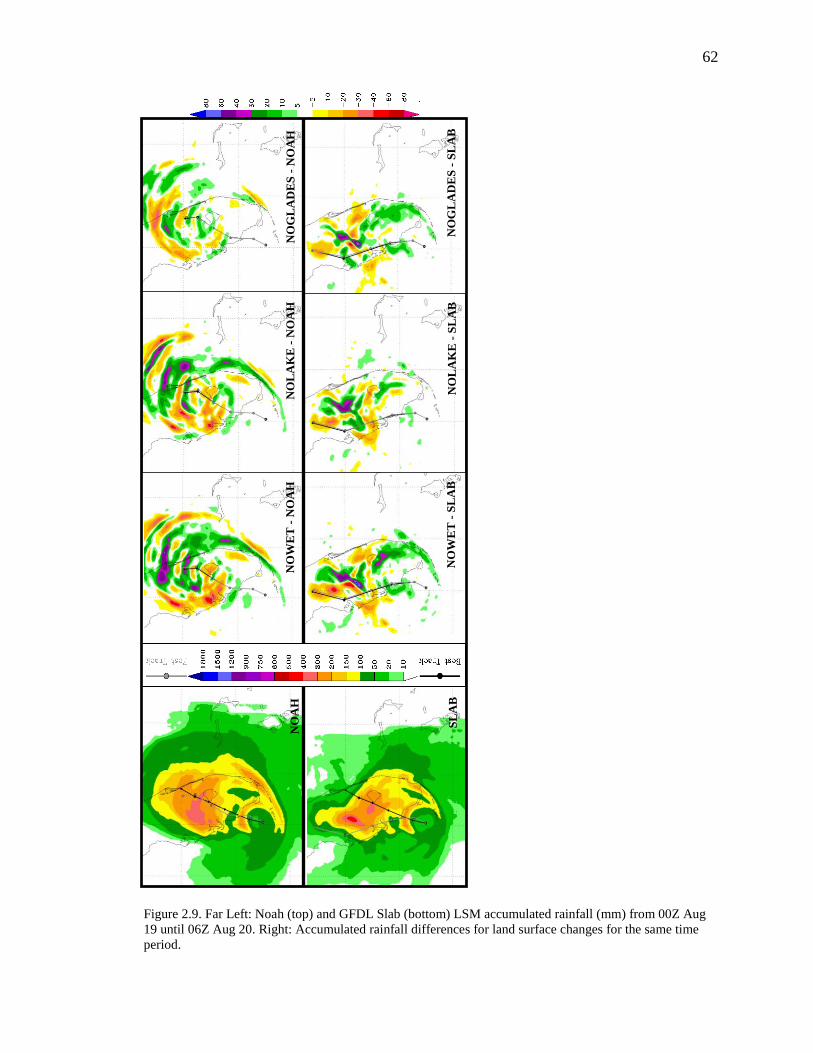
62

62

Figure 2.9. Far Left: Noah (top) and GFDL Slab (bottom) LSM accumulated rainfall (mm) from 00Z Aug

19 until 06Z Aug 20. Right: Accumulated rainfall differences for land surface changes for the same time

period.

NO

WE

T -

NO

AH

N

OA

H

SL

AB

N

OW

ET

- S

LA

B

NO

LA

KE

- N

OA

H

NO

GL

AD

ES

- N

OA

H

NO

LA

KE

- S

LA

B

NO

GL

AD

ES

- S

LA

B

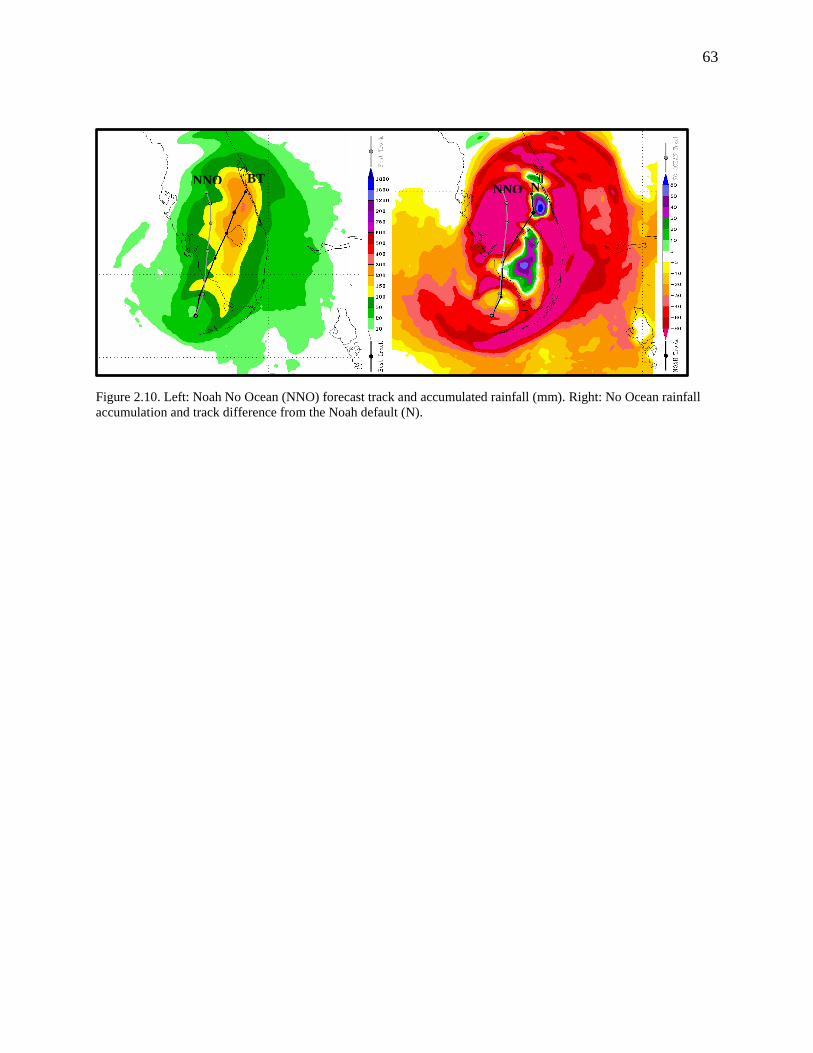
63

63

Figure 2.10. Left: Noah No Ocean (NNO) forecast track and accumulated rainfall (mm). Right: No Ocean rainfall

accumulation and track difference from the Noah default (N).

N NNO BT NNO

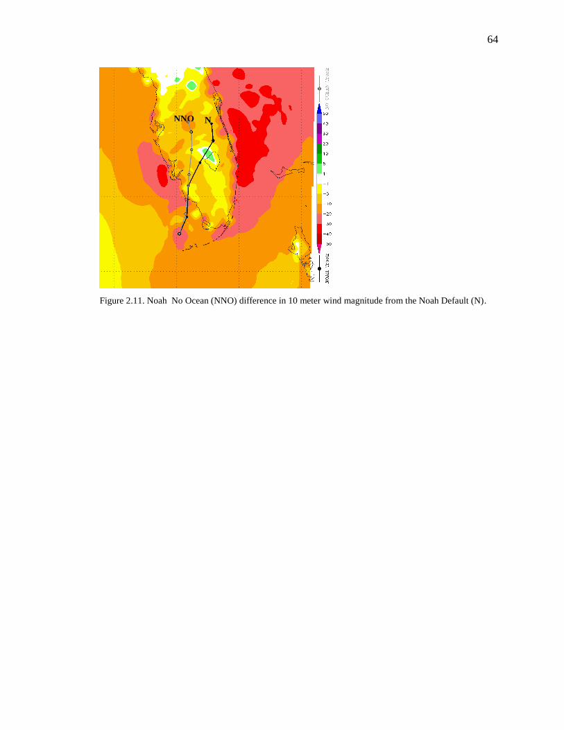
64

64

Figure 2.11. Noah No Ocean (NNO) difference in 10 meter wind magnitude from the Noah Default (N).

NNO N

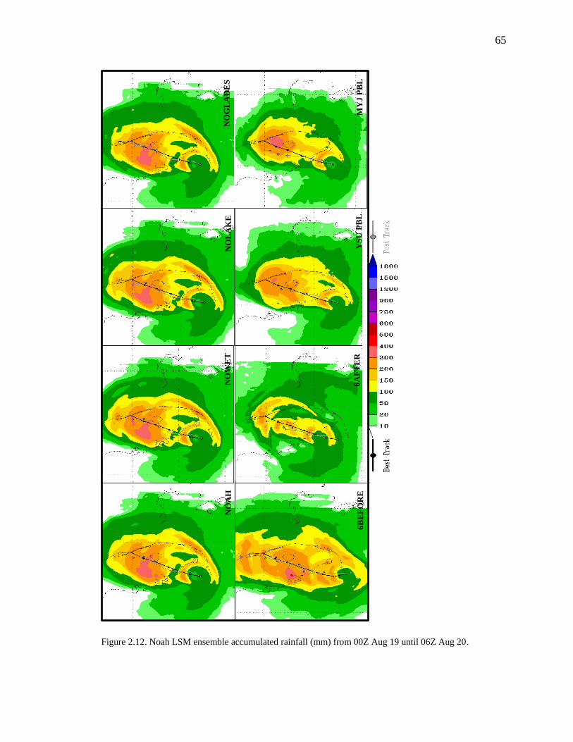
65

65

Figure 2.12. Noah LSM ensemble accumulated rainfall (mm) from 00Z Aug 19 until 06Z Aug 20.

N

OA

H

6B

EF

OR

E

6A

FT

ER

NO

WE

T

MY

J P

BL

NO

GL

AD

ES

N

OL

AK

E

YS

U P

BL

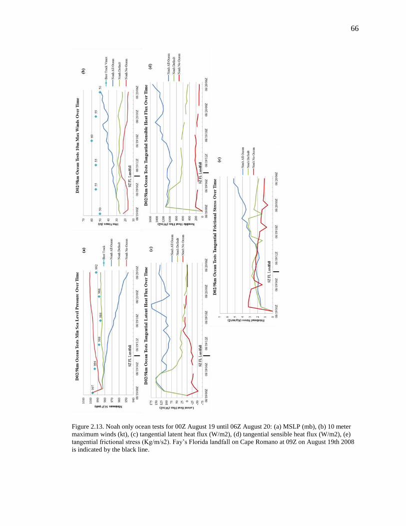
66

66

Figure 2.13. Noah only ocean tests for 00Z August 19 until 06Z August 20: (a) MSLP (mb), (b) 10 meter

maximum winds (kt), (c) tangential latent heat flux (W/m2), (d) tangential sensible heat flux (W/m2), (e)

tangential frictional stress (Kg/m/s2). Fay‟s Florida landfall on Cape Romano at 09Z on August 19th 2008

is indicated by the black line.

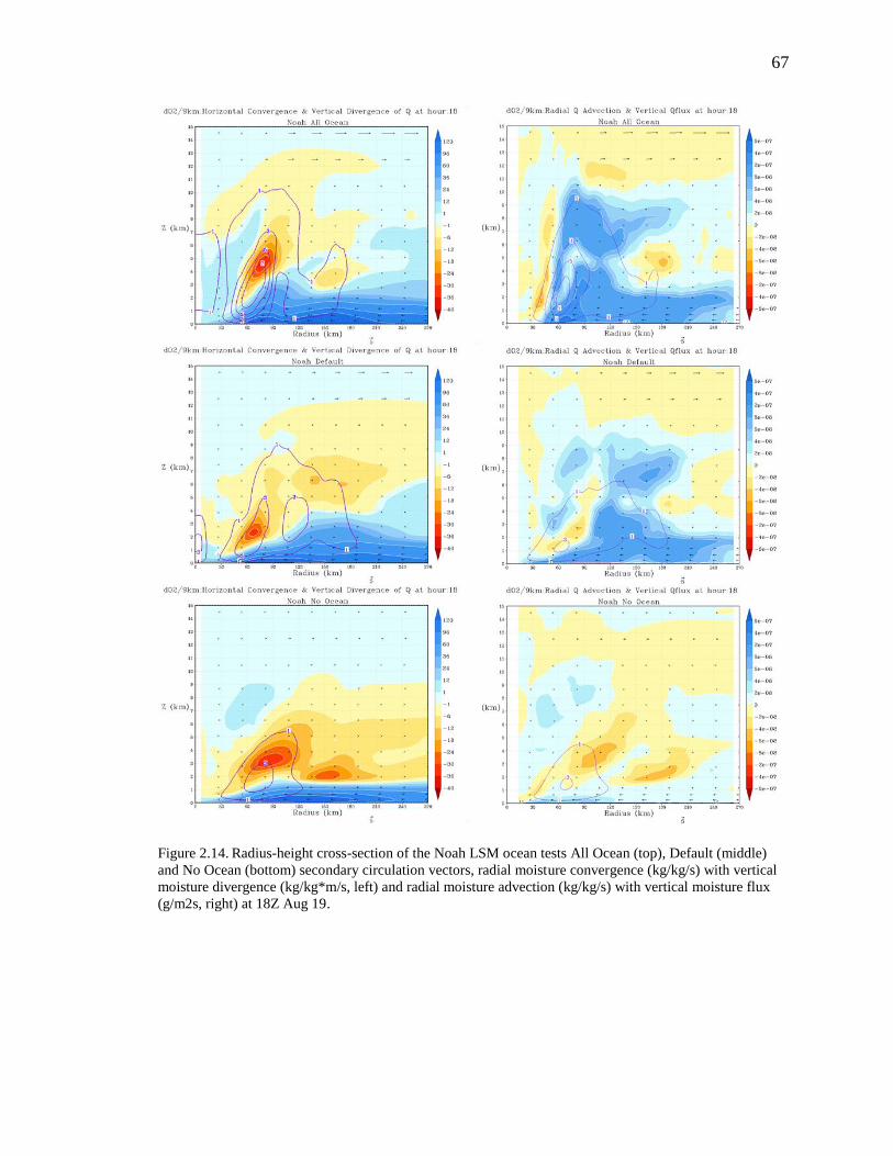
67

67

Figure 2.14. Radius-height cross-section of the Noah LSM ocean tests All Ocean (top), Default (middle)

and No Ocean (bottom) secondary circulation vectors, radial moisture convergence (kg/kg/s) with vertical

moisture divergence (kg/kg*m/s, left) and radial moisture advection (kg/kg/s) with vertical moisture flux

(g/m2s, right) at 18Z Aug 19.

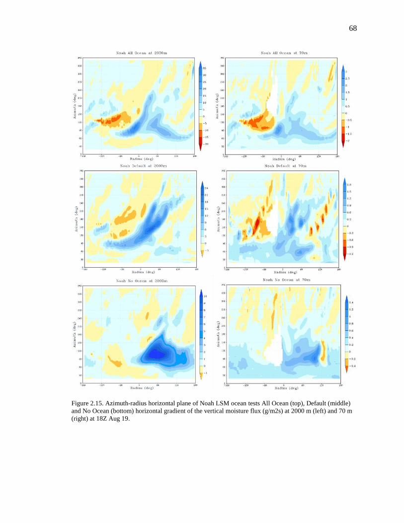
68

68

Figure 2.15. Azimuth-radius horizontal plane of Noah LSM ocean tests All Ocean (top), Default (middle)

and No Ocean (bottom) horizontal gradient of the vertical moisture flux (g/m2s) at 2000 m (left) and 70 m

(right) at 18Z Aug 19.

LIST OF REFERENCES

69

69

LIST OF REFERENCES

Arndt, D. S., J. B. Basara, R. A. McPherson, B. G. Illston, G. D. McManus, and D. B.

Demko, 2009: Observations of the overland reintensification of Tropical Storm

Erin (2007). Bull. Amer. Meteor. Soc., 90, 1079–1093.

Baker, R. D., B. H. Lynn, A. Boone, W. Tao, and J. Simpson, 2001: The influence of soil

moisture, coastline curvature, and land-breeze circulations on sea-breeze-initiated

precipitation. J. Hydrometeor., 2, 193-211.

Bao, S., R. Yablonsky, D. Stark, L. Bernardet, 2010: HWRF User‟s Guide. The

Developmental Testbed Center, Boulder, CO, 88pp.

Bassill, N. P., and M. C. Morgan, 2006: The overland reintensification of Tropical Storm

Danny (1997). Preprints, 27th Conf. on Hurricanes and Tropical Meteorology,

Monterey, CA, Amer. Meteor. Soc., 6A.6.

Bosart, L. F., and G. M. Lackmann, 1995: Postlandfall tropical cyclone reintensification

in a weakly baroclinic environment: A case study of Hurricane David (September

1979). Mon. Wea. Rev., 123, 3268-3291.

Bosart, L. F., and J. A. Bartlo, 1991: Tropical storm formation in a baroclinic

environment. Mon. Wea. Rev., 119, 1979–2013.

Boybeyi, Z. and S. Raman, 1992: A three-dimensional numerical sensitivity study of

convection over the Florida peninsula. Bound.-Layer Meteorol., 60, 325-359.

70

70

Braun, S. A., 2006: High-resolution simulation of Hurricane Bonnie (1998). Part II:

Water budget. J. Atmos. Sci., 63, 43-64.

Chang, H., D. Niyogi, A. Kumar, C. Kishtawal, J. Dudhia, F. Chen, U. C. Mohanty, and

M. Sheperd, 2009: Possible relation between land surface feedback and the post-

landfall structure of monsoon depression. Geophys. Res. Lett., 36 (L15826), 1-6.

Chen, F. and Coauthors, 2006: Description of the characteristics of the NCAR high-

resolution land data assimilation system. J. Appl. Meteorol. Climatol., 46, 694-

713.

Dastoor, A., and T. N. Krishnamurti, 1991: The landfall and structure of a tropical

cyclone: The sensitivity of model predictions to soil moisture parameterizations.

Bound.-Layer Meteorol., 55, 345-380.

Deardorff, J. W., 1978: Efficient prediction of ground surface temperature and moisture,

with inclusion of a layer of vegetation. J. Geophys. Res., 83, 1889-1903.

Ek, M. B., K. E. Mitchell, Y. Lin, E. Rodgers, P. Grunmann, V. Koren, G. Gayno, and J.

D. Tarpley, 2003: Implementation of the Noah land surface model advances in the

NCEP operational mesoscale Eta model. J. Geophys. Res., 108(D22), doi:

10.1029/2002JD003296.

Emanuel, K. A., J. Callaghan, and P. Otto, 2008: A hypothesis for the re-development of

warm-core cyclones over northern Australia. Mon. Wea. Rev., 136, 3863–3872.

Estoque, M. A., 1962: Vertical and radial motions in a tropical cyclone. Tellus, 14(4),

394-400.

71

71

Evans, J. L. and R. E. Hart, 2003: Objective indicators for the life cycle evolution of

extratropical transition for Atlantic tropical cyclones. Mon. Wea. Rev., 131, 909-

925.

Ferrier, B.S., 2005: An efficient mixed-phase cloud and precipitation scheme for use in

operational NWP models. Eos., Trans. Amer. Geophys. Union, 86 (Spring

Meeting Suppl.), Abstract A42A-02.

Gamache, J. F., R. A. Houze Jr., and F. D. Marks Jr., 1993: Dual-aircraft investigation of

the inner core of Hurricane Norbert. Part III: Water budget. J. Atmos. Sci., 50(19),

3221-3243.

Gopalakrishnan, S. G., F. Marks, L. Qingfu, T. Marchok, D. Sheinin, N. Surgi, R. Tuleya,

R. Yablonsky, and X. Zhang, 2010: Hurricane Weather Research and Forecasting

(HWRF) model scientific documentation, NOAA/NCAR/Developmental Tech

Center, 75pp. [Available online at

http://www.dtccenter.org/HurrWRF/users/docs/scientific_documents/HWRF_fina

l_2-2_cm.pdf]

----------------------------, X. Zhang, J. Bao, K. Yeh, and R. Atlas, 2011: The experimental

HWRF system: A study on the influence of horizontal resolution on the structure

and intensity changes in tropical cyclones using an idealized framework. Mon.

Wea. Rev., 139, 1762-1784.

Hong, S.-Y., and H.-L. Pan, 1996: Nonlocal boundary layer vertical diffusion in a

medium-range forecast model. Mon. Wea. Rev., 124, 2322-2339.

----------------------------------, 1998: Convective trigger function for a mass-flux cumulus

parameterization scheme. Mon. Wea. Rev., 129, 1164-1178.

72

72

Kehoe, J., S. Raman, and R. Boyles, 2010: characteristics of landfalling tropical cyclones

in North Carolina. Marine Geodesy, 33(4), 394-411.

Kimball, S., 2004: A modeling study of the sensitivity of landfalling hurricanes to surface

evaporation and surface roughness. Extended Abstracts, 26th

Conference on

Hurricanes and Tropical Meteorology, Miami, FL, Amer. Meteor. Soc. 12D.6.

[Available online at http://ams.confex.com/ams/pdfpapers/75662.pdf.]

Knupp, K. R., J. Walters, and M. Biggerstaff, 2005: Doppler profiler and radar

observations of boundary layer variability during the landfall of Tropical Storm

Gabrielle. J. Atmos. Sci., 63, 234-251.

Kuo, H. L., 1965: On formation and intensification of tropical cyclones through latent

heat release by cumulus convection. J. Atmos. Sci., 22, 40-63.

--------------, 1974: Further studies of the parameterization of the influence of cumulus

convection on large-scale flow. J. Atmos. Sci., 31, 1232-1240.

Kurihara, Y., and R. E. Tuleya, 1981: A numerical simulation study on the genesis of a

tropical storm. Mon. Wea. Rev., 109, 1629-1653.

----------------, --------------------, and M. Bender, 1998: The GFDL hurricane prediction

system and its performance in the 1995 hurricane season. Mon. Wea. Rev., 126,

1306-1322.

Lacis, A. A., and J. E. Hansen, 1974: A parameterization for the absorption of solar

radiation in the earth‟s atmosphere. J. Atmos. Sci., 31,118–133.

73

73

Laing, A., and J. L. Evans, 2010: Introduction to Tropical Meteorology, A

Comprehensive Online and Print Textbook. 2nd ed. University Corporation for

Atmospheric Research, [Available online at

http://www.meted.ucar.edu/tropical/textbook]

Liu, Q., N. Surgi, S. Lord, W. S. Wu, D. Parrish, S. Gopalakrishnan, J. Waldrop, and J.

Gamache, 2006: Hurricane initialization in HWRF model. Extended Abstract,

27th Conf. on Hurricanes and Tropical Meteorology, Monterey, CA, Amer.

Meteor. Soc., 8A.2 [Available online at

http://ams.confex.com/ams/27Hurricanes/techprogram/paper_108496.htm]

Lonfat, M., F. D. Marks, and S. Chen, 2004: Precipitation distribution in tropical

cyclones using the Tropical Rainfall Measuring Mission (TRMM) Microwave

Imager: A global perspective. Mon. Wea. Rev., 132,1645-1660.

Marchok, T., R. Rogers, and R. Tuleya, 2007: Validation schemes for tropical cyclone

quantitative precipitation forecasts: evaluation of operational models for U.S.

landfalling cases. Wea. Forecasting, 22, 726-746.

Marks, F. D. Jr., and R. A. Houze Jr., 1987: Inner core structure of Hurricane Alicia from

airborne Doppler radar observations. J. Atmos. Sci., 44(9), 1296-1317.

McBride, J. L., 1981: Observational analysis of tropical cyclone formation. Part III:

Budget analysis. J. Atmos. Sci., 38, 1152-1166.

Monteverdi, J. P., and R. Edwards, 2008: Documentation of the overland reintensification

of Tropical Storm Erin over Oklahoma, August 18, 2007. Preprints, 24th Conf. on

Severe Local Storms, Savannah, GA, Amer. Meteor. Soc., P4.6.

74

74

--------------------, and ----------------, 2010: The redevelopment of a warm core structure

in Erin: A case of inland tropical storm formation. Electron. J. Severe Storms

Meteor., 5(6), 1-18.

Moon, I., I. Ginis, T. Hara, and B. Thomas, 2007: Physics-based parameterization of air-

sea momentum flux at high wind speeds and its impact on hurricane intensity

predictions. Mon. Wea. Rev., 135, 2869-2878.

Noilhan, J., and S. Planton, 1988: A simple parameterization of land surface processes for

meteorological models. Mon. Wea. Rev., 117, 536-549.

Pielke, R., 1974: A three-dimensional numerical model of the sea breezes over south

Florida. Mon. Wea. Rev., 102, 115-139.

-------------, 2001: Influence of the spatial distribution of vegetation and soils on the

prediction of cumulus convective rainfall. Rev. Geophys., 39, 151–177.

Powell, M.D., and S. D. Aberson, 2001: Accuracy of the United States tropical cyclone

landfall forecasts in the Atlantic basin (1976-2000). Bull. Amer. Meteorol. Soc.,

82, 2749-2767.

Rhome, J. R., and S. Raman, 2006: Environmental influences on tropical cyclone

structure and intensity: A review of past and present literature. Indian J. of

Marine Sci., 35(2), 61-74.

Rodgers, R., F. Marks, and T. Marchok, 2009: Tropical cyclone rainfall. Encyclopedia of

Hydrological Sciences, John Wiley and Sons, pp.1-22. doi:

10.1002/0470848944.hsa030.

75

75

Schwarzkopf, M. D., and S. Fels, 1991: The simplified exchange method revisited: An

accurate, rapid method for computation of infrared cooling rates and fluxes. J.

Geophys. Res., 96, 9075-9096.

Shen, W., I. Ginis, and R. E. Tuleya, 2002: A numerical investigation of land surface

water on landfalling hurricanes. J. Atmos. Sci., 59, 789-802.

Singh, R., P. K. Pal, C. M. Kishtawal, and P. C. Joshi, 2005: Impact of bogus vortex for

track and intensity prediction of tropical cyclone. J. Earth Syst. Sci. 114, 427-436.

Sousounis, P. J., and J. M. Fritsch, 1994: Lake-aggregate mesoscale disturbances. Part II:

A case study of the effects on the regional and synoptic-scale weather systems.

Bull. Amer. Meteorol. Soc., 75, 1793-1811.

Stuart, S. R., and J. L. Beven II, 2009: Tropical cyclone report, Tropical Storm Fay, 15-

26 August 2008. Miami, FL: National Hurricane Center. [Available online at

http://www.nhc.noaa.gov/pdf/TCR-AL062008_Fay.pdf]

Tuleya, R. E., and Y. Kurihara, 1978: A numerical simulation of the landfall of tropical

cyclones. J. Atmos. Sci., 35, 242–257.

-----------------, M. A. Bender, and Y. Kurihara, 1984: A simulation study of the landfall

of tropical cyclones using a movable nested-mesh model. Mon. Wea. Rev., 112,

124–136.

-----------------, 1994: Tropical storm development and decay: Sensitivity to surface

boundary conditions. Mon. Wea. Rev., 122, 291–304.

76

76

-----------------, 2010: Test results using the NOAH LSM in the operational HWRF

system. Recorded Presentation, 29th Conference on Hurricanes and Tropical

Meteorology, Tucson, AZ, Amer. Meteor. Soc., 12C.7 [Available online at

http://ams.confex.com/ams/29Hurricanes/techprogram/paper_168976.htm]

Wilson, J. W., and D. L. Megenhardt, 1997: Thunderstorm initiation, organization, and

lifetime associated with Florida boundary layer convergence lines. Mon. Wea.

Rev., 125, 1507-1525.

APPENDIX

77

77

APPENDIX: MODIFICATION OF GEOGRAPHY TILES

To study the contribution of the Florida surface features, idealized HWRF runs

were designed to “remove” the features of interest from the model geography tiles. This

section supplements the earlier description of the geography tile alteration with further

detail, instructions and figures to assist those who wish to attempt this in their own

research projects. WRF model geography tiles are available in a variety of data

resolutions: 10 minute (10m), 2 minute (2m), and 30 seconds (30s). For this example and

experiments, only the hi-resolution 30s data was used in the WPS geogrid program when

defining the static geography in the model domain. Each dataset resolution comes with an

“index” metadata file that documents the data‟s type, resolution, and projection, coverage,

and “known” global latitude and longitude points (Sample A.1). This index file helps the

user determine which tile number holds the data for a specific latitude/longitude pair. In

this case, we are interested in Florida, particularly Lake Okeechobee which is located at

approximately 26.96, -80.80 (ie. 26.96 N, 80.80 W). According to the index file for the

30s data, the dx/dy resolution is 0.00833333 x 0.00833333 and the known

latitude/longitude pair is (-89.99583/-179.99583). To determine which geography tile (in

startXXXXX-endXXXXX.startYYYYY-endYYYYY format) will contain the data for

Lake Okeechobee, we use this formula to determine the tile‟s x (longitude) and y

(latitude) point in the file:

78

78

1008333.099583.89

1008333.099583.179

latitudey

longitudex

For Lake Okeechobee, this becomes approximately x = 11904 and y = 1436. Therefore,

the lake data is located in the “10801-12000.13201-14400” geography tile for the 24-

category USGS landuse and 16-category soil type (for both the soil top (∆Z = 10cm) and

soil bottom (∆Z = 30cm) layer) files. The same process was done for the Florida

Everglades which is located in the same geography tile. Refer to Tables A.1 and A.2 for

the complete category listings of the USGS landuse and soil type categories respectively.

Next, copy the original 10801-12000.13201-14400 binary geography tiles located

in the landuse_30s, soiltype_top_30s, soiltype_bot_30s sub-directories of the geo_static

data download to work with. Since one cannot easily read and edit binary data, a program

must be written to output the data into an ASCII text file that can be read with any text

editor. The Fortran 90 code is needed to do three things: (a) read in all the data in the tile

of choice and write out the original data to a text file for viewing, (b) allow editing of the

variable in question within a particular subsection of the tile data, and (c) either write out

the changed data to a secondary text file for verification of the committed changes to the

data, and/or re-write the edited data back into binary format. Again, looking at the index

file for the dataset, use the tile_x and tile_y variables to determine the dimensions of the

data. For 30s data, the dimensions are 1200 x 1200. The example presented below will

only be for the 24-category USGS landuse data.

To read the data correctly, declare some Fortran variables with the proper format,

knowing the data dimensions discussed earlier and that the data values are represented as

two digits ranging from 1-24 for landuse and 1-16 for soil type (lines 1-8 in the code

79

79

from Sample A.2). Read in the data to the landuse variable to later work with the original

data (lines 9-12). Write the original data out to a text file to view data file contents (lines

13-16). Once the lake has been found (should be a large section of category 16

surrounded by land, where USGS 16 = water), decide on a line number/character number

box surrounding the lake. The line numbers will represent the upper and lower bounds of

the box, while the character numbers represent the eastward and westward boundaries of

the box that surrounds the lake where the changes to the landuse values will occur. In this

case, I chose lines 338 to 397, and character numbers 2158 to 2258 to represent the lake

change box. The Florida Everglades box includes lines 412 to 610 and characters 1910 to

2396. The box for the lake is represented as the blue dashed box in the top panel of

Figure A.1, the box surrounding the Florida Everglades is represented as the green

dashed box also in Figure A.1. However, to determine the lake box within the binary data,

one needs to take into account the tile_x = 1200 and tile_y = 1200 data dimensions with

the formulas below:

2/)(

2/)(

1)(1200

1)(1200

Eastcharright

Westcharleft

Southlinebottom

Northlinetop

For the top and bottom extremes, we designate 1200 minus the line number since the data

is being printed to the text file in reverse order. The resulting numbers will serve as the

appropriate boundary box for Lake Okeechobee in the binary data (lines 17-25); in this

case: ix >= 1080 and ix <= 1128, iy >= 804 and iy<= 863 where the default landuse is

equal to category 16 (line 20). For the Everglades, the data box is equal to: ix >= 955 and

ix >= 1198, iy >= 591 and iy <= 789 where the default landuse is equal to category 18

80

80

(USGS 18 = wooded wetland). Temporarily change the lake values to “99” (line 21) and

write out the temporary data to another text file to verify that only the lake data was

changed (lines 26-29). To change the lake to the final values, uncomment out line 22 in

order to switch the lake values from water (16) to dryland/cropland and pasture (2). Once

satisfied with the output, write the text data back out to a binary file so that WPS can read

it (lines 30-34). The changed values for both Lake Okeechobee and the Everglades are

displayed in Figure A.2. This representation of the landuse (top panel), soil type top layer

(middle panel), and soil type bottom layer (bottom panel) in Figures 1a and 1b are the

actual values used in the Noah default (N) and Noah NOWET (NW) model runs

respectively. The goal of altering these surface variables is to attempt to dry out the land

surface by using soil with reduced water storage capacity, and landuse or vegetation that

is characterized by a higher roughness length and reduced moisture values. The values in

the Noah NOLAKE (NL) and Noah NOGLADES (NG) would be represented by only

one of the land features being altered in the panels of Figure A.2. Values for the Noah

NOOCEAN (NNO) would include the default values for the lake and Everglades,

however with the ocean body changed to category 6: cropland/woodland mosaic, 1: sand,

and 1: sand for the landuse, soil top and bottom respectively. The Noah ALLOCEAN run

(NAO) would just be the water category for all variables for every x and y point in the

text file.

81

81

Sample A.1. Example Index file for the USGS Landuse Tile containing data for Lake Okeechobee.

type=categorical

category_min=1

category_max=24

projection=regular_ll

dx=0.00833333

dy=0.00833333

known_x=1.0

known_y=1.0

known_lat=-89.99583

known_lon=-179.99583

wordsize=1

tile_x=1200

tile_y=1200

tile_z=1

units="category"

description="24-category USGS landuse"

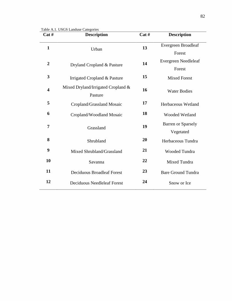
82

82

Table A.1. USGS Landuse Categories

Cat # Description Cat # Description

1 Urban 13 Evergreen Broadleaf

Forest

2 Dryland Cropland & Pasture 14 Evergreen Needleleaf

Forest

3 Irrigated Cropland & Pasture 15 Mixed Forest

4 Mixed Dryland/Irrigated Cropland &

Pasture

16 Water Bodies

5 Cropland/Grassland Mosaic 17 Herbaceous Wetland

6 Cropland/Woodland Mosaic 18 Wooded Wetland

7 Grassland 19 Barren or Sparsely

Vegetated

8 Shrubland 20 Herbaceous Tundra

9 Mixed Shrubland/Grassland 21 Wooded Tundra

10 Savanna 22 Mixed Tundra

11 Deciduous Broadleaf Forest 23 Bare Ground Tundra

12 Deciduous Needleleaf Forest 24 Snow or Ice

83

83

Table A.2. Soil Type Categories

Cat # Description Cat # Description

1 Sand 9 Clay Loam

2 Loamy Sand 10 Sandy Clay

3 Sandy Loam 11 Silty Clay

4 Silt Loam 12 Clay

5 Silt 13 Organic Materials

6 Loam 14 Water

7 Sandy Clay Loam 15 Bedrock

8 Silty Clay Loam 16 Other (land-ice)

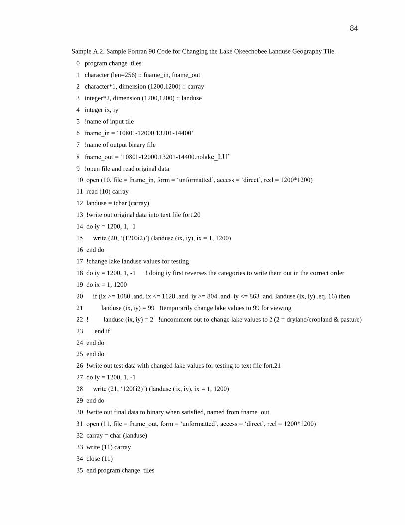
84

84

Sample A.2. Sample Fortran 90 Code for Changing the Lake Okeechobee Landuse Geography Tile.

0 program change_tiles

1 character (len=256) :: fname_in, fname_out

2 character*1, dimension (1200,1200) :: carray

3 integer*2, dimension (1200,1200) :: landuse

4 integer ix, iy

5 !name of input tile

6 fname_in = „10801-12000.13201-14400‟

7 !name of output binary file

8 fname_out = „10801-12000.13201-14400.nolake_LU‟

9 !open file and read original data

10 open (10, file = fname_in, form = „unformatted‟, access = „direct‟, recl = 1200*1200)

11 read (10) carray

12 landuse = ichar (carray)

13 !write out original data into text file fort.20

14 do iy = 1200, 1, -1

15 write (20, „(1200i2)‟) (landuse (ix, iy), ix = 1, 1200)

16 end do

17 !change lake landuse values for testing

18 do iy = 1200, 1, -1 ! doing iy first reverses the categories to write them out in the correct order

19 do ix = 1, 1200

20 if (ix >= 1080 .and. ix <= 1128 .and. iy >= 804 .and. iy <= 863 .and. landuse (ix, iy) .eq. 16) then

21 landuse (ix, iy) = 99 !temporarily change lake values to 99 for viewing

22 ! landuse (ix, iy) = 2 !uncomment out to change lake values to 2 (2 = dryland/cropland & pasture)

23 end if

24 end do

25 end do

26 !write out test data with changed lake values for testing to text file fort.21

27 do iy = 1200, 1, -1

28 write (21, „1200i2)‟) (landuse (ix, iy), ix = 1, 1200)

29 end do

30 !write out final data to binary when satisfied, named from fname_out

31 open (11, file = fname_out, form = „unformatted‟, access = „direct‟, recl = 1200*1200)

32 carray = char (landuse)

33 write (11) carray

34 close (11)

35 end program change_tiles

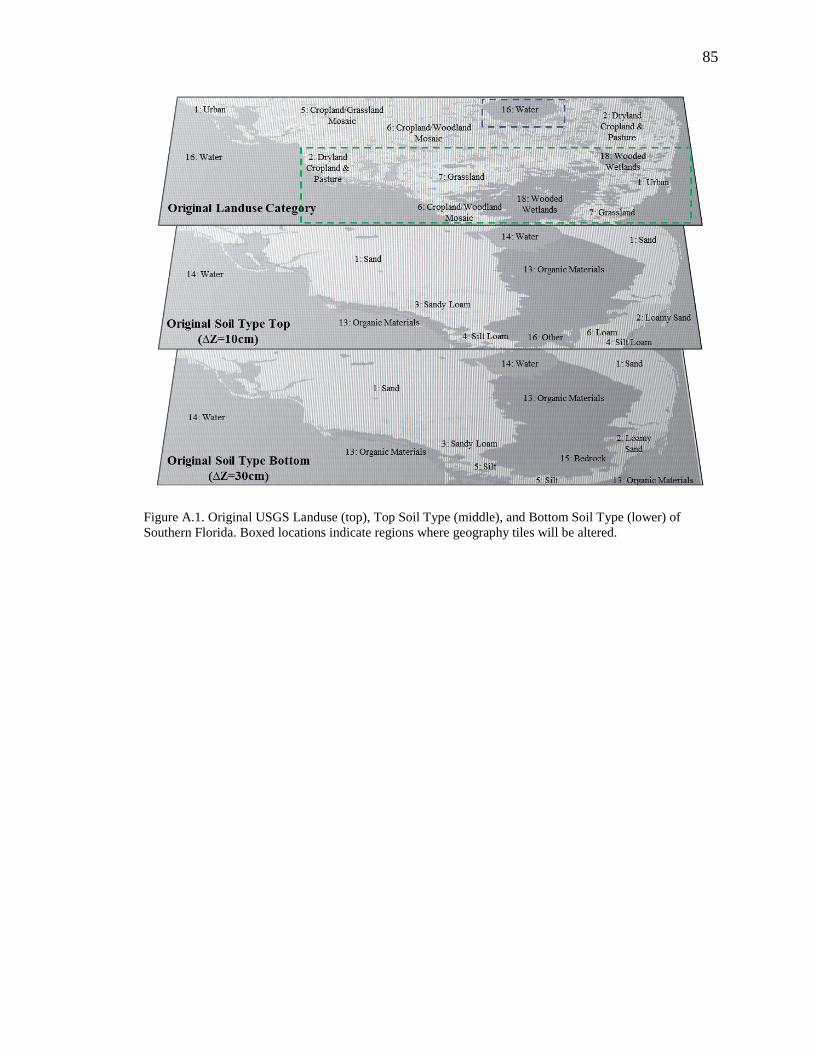
85

85

Figure A.1. Original USGS Landuse (top), Top Soil Type (middle), and Bottom Soil Type (lower) of

Southern Florida. Boxed locations indicate regions where geography tiles will be altered.

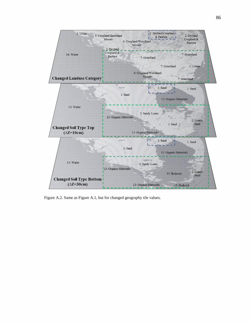
86

86

Figure A.2. Same as Figure A.1, but for changed geography tile values.

VITA

87

87

VITA

Monica Laureano Bozeman

Earth and Atmospheric Sciences Department, Purdue University

Education

B.S., Meteorology, Environmental Science Minor, 2009, North Carolina State University,

Raleigh, North Carolina

M.S., Atmospheric Science, 2011, Purdue University, West Lafayette, Indiana

Thesis: Land Surface Feedbacks on the Post-landfall Tropical Cyclone

Characteristics using the Hurricane Weather Research and Forecasting (HWRF)

Modeling System.

Publications

1. Bozeman, M. L., D. Niyogi, S. Gopalakrishnan, F. Marks Jr., X. Zhang, and V.

Tallapragada, 2011: An HWRF Based - Ensemble Assessment of Possible Land

Surface Feedbacks on the Post-Landfall Intensification of Tropical Storm Fay of

2008. Natural Hazards. doi: 10.1007/s11069-011-9841-5

2. Kishtawal, M., D. Niyogi, A. Kumar, M. Laureano and O. Kellner 2011:

Sensitivity of Inland Decay of North Atlantic Tropical Cyclones to Soil

Parameters. Natural Hazards.

Presentations

1. November 2010: An HWRF Examination of Land Surface Influence on Fay.

Monthly Modeling Group Meeting, Atlantic and Oceanographic Meteorological

Laboratory-Miami, FL.

2. August 2010: An Introduction to the Hurricane WRF (HWRF) NWP Model. State

Climate Office of North Carolina-Raleigh, NC.

3. August 2010: Land Surface Heterogeneity Effects on HWRF forecasts of Tropical

Storm Fay. Monthly Modeling Group Meeting, Atlantic and Oceanographic

Meteorological Laboratory-Miami, FL.

4. July 2010: LSM Sensitivity of HWRF on Tropical Storm Fay storm track and

forecasts. Monthly Modeling Group Meeting, Atlantic and Oceanographic

Meteorological Laboratory-Miami, FL.

88

88

Skills

Operating Systems: Windows XP and 2000, Linux/Unix

Scripting Languages: C-shell, JAVA, JavaScript, Perl, PHP, MySQL, HTML

Software: Microsoft Office Professional 2003 & 2007, GEMPAK-General Meteorology

Package, GrADS, NCL, GARP, IDV, wrfpost, MET-Model Evaluation Tool, Google

Visualization API, SolidWorks

Professional affiliations

American Meteorological Society, Student Member

Alumni of the Purdue Women in Science Program (WISP)

Alumni of the NCSU Women in Science and Engineering (WISE) Program

PUBLICATION

89

89

PUBLICATION

Sensitivity of inland decay of North Atlantic tropical cyclones to soil parameters2

Chandra M. Kishtawal, Dev Niyogi, Anil Kumar*, Monica Laureano, Olivia Kellner

Purdue University, Department of Agronomy and Department of Earth and Atmospheric

Sciences, West Lafayette, IN-47907, USA

*also with ESSIC University of Maryland, College Park, MD and NASA/GSFC

Hydrological Science Branch.

Abstract

Using the HURDAT best track analysis of track and intensity of tropical cyclones that

made landfall over the continental United States during the satellite era (1980-2005), we

analyze the role of land surface variables on the cyclone decay process. The land surface

variables considered in the present study, included soil parameters (soil heat capacity and

soil bulk density), roughness, topography and local gradients of topography. The

sensitivity analysis was carried out using a data-adaptive genetic algorithm approach that

automatically selects the most suitable variable by fitting optimum empirical functions

that estimates cyclone intensity decay in terms of given observed variables. Analysis

indicates that soil bulk density (a surrogate for soil heat capacity) has a dominant

influence on cyclone decay process. The decayed inland cyclone intensities were found to

2 Publication abstract reproduced with permission from Dr. Dev Niyogi. Citation: Kishtawal, A., D. Niyogi,

A. Kumar, M. Laureano, O. Kellner 2011: Sensitivity of inland decay of North Atlantic tropical cyclones to

soil parameters. Natural Hazards. in press.

90

90

be positively correlated to the cube of the soil bulk density. The impact of the changes in

soil bulk density on the decayed cyclone intensity is higher for higher intensity cyclone

Since soil bulk density is closely related to the soil heat capacity, and inversely

proportional to the thermal diffusivity, the observed relationship can also be viewed as

the influence of cooling rate of the land surface, as well as the transfer of heat and

moisture underneath a landfalling storm. The optimized prediction function obtained by

statistical model process in the present study that predicts inland intensity changes during

6h interval, showed high fitness index, and small errors. The performance of the

prediction function was tested on inland tracks of eighteen hurricanes and tropical storms

that made landfall over the United States between 2001-2010. The mean error of intensity

prediction for these cyclones varied from 1.3 to 15.8 knots (0.67 to 8.12 m s-1

). Results

from the data driven analysis thus indicate that soil heat flux feedback should be an

important consideration for the inland decay of tropical cyclones. Experiments were also

undertaken with Weather Research Forecasting (WRF) Advanced Research Version

(ARW ver 3.3) to assess the sensitivity of the soil parameters (roughness, heat capacity,

and bulk density) on the post land fall structure of select storms. The model was run with

1 km grid spacing, limited area single domain with boundary conditions from the North

American Regional Reanalysis. Of the different experiments only the surface roughness

change and soil bulk density (heat capacity) change experiments showed some sensitivity

to the intensity change. The WRF results thus have a low sensitivity to the land

parameters (with only the roughness length showing some impact). This calls for

reassessing the land surface response on postlandfall characteristics with more detailed

land surface representation within the mesoscale and hurricane modeling systems.

Keywords: Tropical Cyclone, Landfalling Cyclones, Hurricane Intensity, Land Surface

Feedback, Soil Heat Flux, Inland Decay.