Laplace Inversion of Low-Resolution NMR Relaxometry …web.stanford.edu/group/SOL/papers/CMR21263.pdf · Laplace Inversion of ... Relaxometry Data Using Sparse Representation Methods

Laplace Inversion ofLow-Resolution NMRRelaxometry Data UsingSparse RepresentationMethodsPAULA BERMAN,1 OFER LEVI,2 YISRAEL PARMET,2 MICHAEL SAUNDERS,3 ZEEV WIESMAN1

1The Phyto-Lipid Biotechnology Laboratory, Departments of Biotechnology and Environmental Engineering,The Institutes for Applied Research, Ben-Gurion University of the Negev, Beer-Sheva, Israel2Department of Industrial Engineering and Management, Ben-Gurion University of the Negev, Beer-Sheva, Israel3Department of Management Science and Engineering, Stanford University, Stanford, CA

ABSTRACT: Low-resolution nuclear magnetic resonance (LR-NMR) relaxometry is a

powerful tool that can be harnessed for characterizing constituents in complex materials.

Conversion of the relaxation signal into a continuous distribution of relaxation compo-

nents is an ill-posed inverse Laplace transform problem. The most common numerical

method implemented today for dealing with this kind of problem is based on L2-norm

regularization. However, sparse representation methods via L1 regularization and convex

optimization are a relatively new approach for effective analysis and processing of digital

images and signals. In this article, a numerical optimization method for analyzing LR-

NMR data by including non-negativity constraints and L1 regularization and by applying

a convex optimization solver PDCO, a primal-dual interior method for convex objectives,

that allows general linear constraints to be treated as linear operators is presented. The

integrated approach includes validation of analyses by simulations, testing repeatability

of experiments, and validation of the model and its statistical assumptions. The pro-

posed method provides better resolved and more accurate solutions when compared

with those suggested by existing tools. VC 2013 Wiley Periodicals, Inc. Concepts Magn

Reson Part A 42A: 72–88, 2013.

KEY WORDS: low-resolution NMR; sparse reconstruction; L1 regularization; convex

optimization

Received 16 March 2013; accepted 1 April 2013

Correspondence to: Zeev Wiesman; (E- mail: [email protected])

Concepts in Magnetic Resonance Part A, Vol. 42A(3) 72–88 (2013)

Published online in Wiley Online Library (wileyonlinelibrary.com).DOI: 10.1002/cmr.a.21263

� 2013 Wiley Periodicals, Inc.

72

I. INTRODUCTION

Low-resolution nuclear magnetic resonance (LR-

NMR) relaxometry has emerged as a powerful new

tool for identifying molecular species and to study their

dynamics even in complex materials. This technology

is widely used in industrial quality control for the deter-

mination of solid-to-liquid and oil-to-water ratios in

materials as diverse as oil-bearing rock, food emul-

sions, and plant seeds (1). It offers great potential for

characterization and ultimately quantification of com-

ponents in different materials in their whole conforma-

tion. Many recent developments are reviewed by

Bl€umich et al. (2). Note that the term LR-NMR is used

in other contexts such as time-domain NMR, ex situ

NMR, and portable NMR.

The process of relaxation occurs as a consequence

of interactions among nuclear spins and between

them and their surroundings. In biological samples,

spins exist in a variety of different environments, giv-

ing rise to a spectrum of relaxation times, where the

measured relaxation decay is a sum of contributions

from all spins (3). Spin–spin interactions are the main

relaxation mechanism in a CPMG (Carr, Purcell, Mei-

boom and Gill) pulse sequence (4,5).

Conversion of the relaxation signal into a continu-

ous distribution of relaxation components is an ill-

posed inverse Laplace transform (ILT) problem. The

probability density f(T2) is calculated as follows:

s tð Þ5ð10

e2t=T2 f T2ð ÞdT21E tð Þ; (1)

where s(t) is the relaxation signal acquired with LR-

NMR at time t; T2 denotes the time constants; and E(t)is the measurements error.

Istratov and Vyvenko (6) reviewed the fundamentals

and limitations of the ILT. The most common numeri-

cal method implemented today for dealing with ill-

posed problems of this kind is based on L2-norm regu-

larization (3,7–9), where Eq. [1] is approximated by a

discretized matrix form and optimized according to the

following equation:

f5 arg minf�0

||s2Kf ||221 k || f ||22; (2)

where K is the discrete Laplace transform and k is the

L2 weight. This type of regularization, however, can

significantly distort the solution by contributing to the

broadening of peaks.

It should be noted that the non-negativity constraint

in Eq. [2] makes the problem much harder to solve.

Without the constraint, a standard least-squares (LS)

solver can be applied. The solution f obtained will sat-

isfy the related normal equation:

KTK1 k I� �

f 5KTs; (3)

However, there is no guarantee that f will be non-

negative even if negative components are not physi-

cally feasible, as in the LR-NMR case. In practice, it is

not acceptable to set negative values to zero. To solve

Eq. [2], optimally, we need more sophisticated optimi-

zation tools such as interior-point methods (10).

Sparse representation methods are a relatively new

approach for analysis and processing of digital images

and signals (11). State-of-the-art optimization tools are

used to handle efficiently even highly underdetermined

systems. The main feature of these methods lies in

using L1 regularization in addition to the common L2

regularization. It has been shown in theory and in prac-

tice that the L1 norm is closely related to the sparsity of

signals (12). The L1 norm of the solution is the sum of

absolute values of its components. Absolute value

terms in the objective function are harder to handle

than quadratic terms. However, it is possible to state

the L1-regularized problem as a convex optimization

problem and then use an appropriate convex optimiza-

tion solver. Typically, such solvers can handle the non-

negativity constraint.

In this work, we apply advanced sparse representa-

tion tools to the problem of LR-NMR relaxometry. We

use PDCO, a primal-dual interior method for convex

objectives (13). PDCO can be adjusted to solve the LR-

NMR relaxometry inverse problem with non-negativity

constraints and an L1 regularization term that stabilizes

the solution process without introducing the typical L2

peak broadening. Our new suggested method makes it

possible to resolve close adjacent peaks, whereas exist-

ing tools typically fail, as we demonstrate below.

The underlying principle is that all structured signals

have sparse representation in an appropriate coordinate

system, and using such a system/dictionary typically

results in better solutions when the noise level is rela-

tively low. Evidently, one of the most important ele-

ments of this approach is choosing an appropriate

dictionary.

II. THE LR-NMR DISCRETE INVERSEPROBLEM

Inverse problems and their solutions are of great impor-

tance in many disciplines. Application fields include

medical and biological imaging, radar, seismic imag-

ing, nondestructive testing, and more. An inverse prob-

lem is typically related to a physical system that can

LAPLACE INVERSION OF LR-NMR RELAXOMETRY DATA 73

Concepts in Magnetic Resonance Part A (Bridging Education and Research) DOI 10.1002/cmr.a

take indirect measurements s of some unknown func-

tion f. The relationship between s and f is determined

by the characteristics of the measurement system and

relevant physical principles.

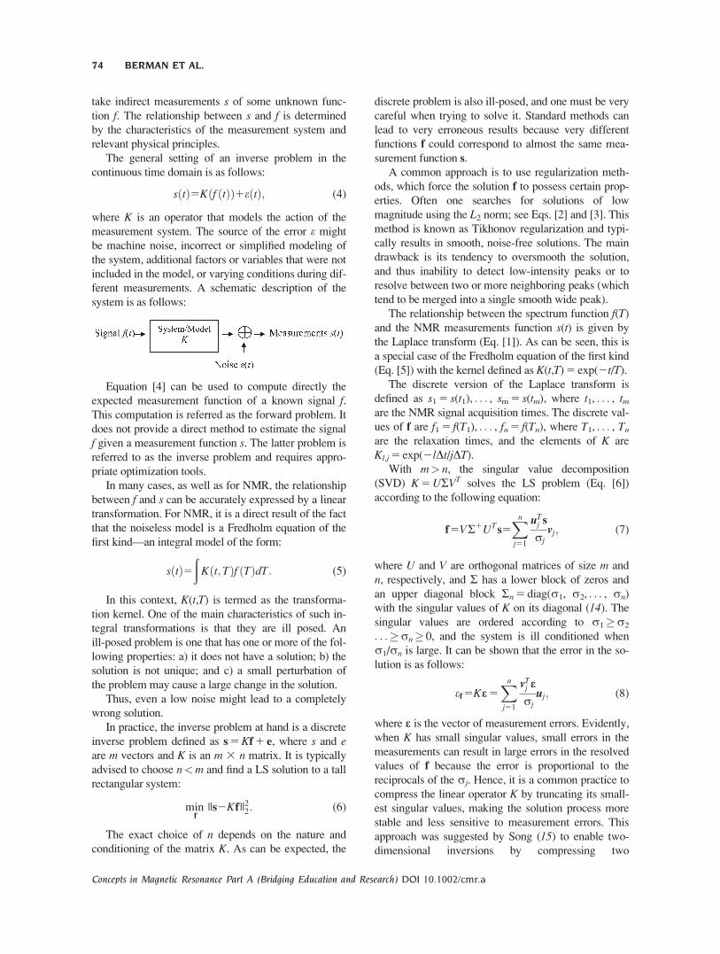
The general setting of an inverse problem in the

continuous time domain is as follows:

sðtÞ5Kðf ðtÞÞ1e tð Þ; (4)

where K is an operator that models the action of the

measurement system. The source of the error e might

be machine noise, incorrect or simplified modeling of

the system, additional factors or variables that were not

included in the model, or varying conditions during dif-

ferent measurements. A schematic description of the

system is as follows:

Equation [4] can be used to compute directly the

expected measurement function of a known signal f.This computation is referred as the forward problem. It

does not provide a direct method to estimate the signal

f given a measurement function s. The latter problem is

referred to as the inverse problem and requires appro-

priate optimization tools.

In many cases, as well as for NMR, the relationship

between f and s can be accurately expressed by a linear

transformation. For NMR, it is a direct result of the fact

that the noiseless model is a Fredholm equation of the

first kind—an integral model of the form:

s tð Þ5ð

K t; Tð Þf Tð ÞdT: (5)

In this context, K(t,T) is termed as the transforma-

tion kernel. One of the main characteristics of such in-

tegral transformations is that they are ill posed. An

ill-posed problem is one that has one or more of the fol-

lowing properties: a) it does not have a solution; b) the

solution is not unique; and c) a small perturbation of

the problem may cause a large change in the solution.

Thus, even a low noise might lead to a completely

wrong solution.

In practice, the inverse problem at hand is a discrete

inverse problem defined as s 5 Kf 1 e, where s and eare m vectors and K is an m 3 n matrix. It is typically

advised to choose n<m and find a LS solution to a tall

rectangular system:

minf

||s2Kf ||22: (6)

The exact choice of n depends on the nature and

conditioning of the matrix K. As can be expected, the

discrete problem is also ill-posed, and one must be very

careful when trying to solve it. Standard methods can

lead to very erroneous results because very different

functions f could correspond to almost the same mea-

surement function s.

A common approach is to use regularization meth-

ods, which force the solution f to possess certain prop-

erties. Often one searches for solutions of low

magnitude using the L2 norm; see Eqs. [2] and [3]. This

method is known as Tikhonov regularization and typi-

cally results in smooth, noise-free solutions. The main

drawback is its tendency to oversmooth the solution,

and thus inability to detect low-intensity peaks or to

resolve between two or more neighboring peaks (which

tend to be merged into a single smooth wide peak).

The relationship between the spectrum function f(T)

and the NMR measurements function s(t) is given by

the Laplace transform (Eq. [1]). As can be seen, this is

a special case of the Fredholm equation of the first kind

(Eq. [5]) with the kernel defined as K(t,T) 5 exp(2t/T).

The discrete version of the Laplace transform is

defined as s1 5 s(t1), . . . , sm 5 s(tm), where t1, . . . , tmare the NMR signal acquisition times. The discrete val-

ues of f are f1 5 f(T1), . . . , fn 5 f(Tn), where T1, . . . , Tn

are the relaxation times, and the elements of K are

Kl,j 5 exp(2lDt/jDT).

With m> n, the singular value decomposition

(SVD) K 5 URVT solves the LS problem (Eq. [6])

according to the following equation:

f5VR1UTs5Xn

j51

uTj s

rjvj; (7)

where U and V are orthogonal matrices of size m and

n, respectively, and R has a lower block of zeros and

an upper diagonal block Rn 5 diag(r1, r2, . . . , rn)

with the singular values of K on its diagonal (14). The

singular values are ordered according to r1�r2

. . .�rn� 0, and the system is ill conditioned when

r1/rn is large. It can be shown that the error in the so-

lution is as follows:

ef5Ke 5Xn

j51

vTj e

rjuj; (8)

where e is the vector of measurement errors. Evidently,

when K has small singular values, small errors in the

measurements can result in large errors in the resolved

values of f because the error is proportional to the

reciprocals of the rj. Hence, it is a common practice to

compress the linear operator K by truncating its small-

est singular values, making the solution process more

stable and less sensitive to measurement errors. This

approach was suggested by Song (15) to enable two-

dimensional inversions by compressing two

74 BERMAN ET AL.


one-dimensional inversion matrices before constructing

the larger two-dimensional matrix. (Tikhonov regulari-

zation is still typically necessary.) The best rank-rapproximation to K is the partial sum of the first r SVD

components:Xr

j51rjujv

Tj : This compression stabil-

izes the solution while making a relatively small pertur-

bation to the original problem defined by K.

Apparently, both L2 regularization and SVD com-

pression could be applied to improve the condition and

stability of the inverse problem as well as to reduce the

level of noise in the solution. There is an interesting

relationship between the two methods: the L2 regulari-

zation in Eq. [2] is equivalent to applying multiplica-

tive weights to the singular values of K, where the

weights are given by w(r) 5 r2/(r2 1 k) (16), and

therefore, the larger singular values become more dom-

inant. Thus, L2 regularization is equivalent to smooth

damping of the small singular values, whereas the

SVD compression applies sharp truncation to the sin-

gular value series.

Other approaches for the NMR spectrum recon-

struction include Monte Carlo simulation inversion

(17), where an entire family of probable solutions are

for a given measurements set. In addition, in Ref. (18),

a phase analysis is applied to the measurements func-

tion using the Fourier transform to evaluate the expo-

nential decay rates.

Herrholz and Teschke (19) considered sparse ap-

proximate solutions to ill-posed inversion problems,

using compressed sensing methods, Tikhonov regulari-

zation, and possibly infinite-dimensional reconstruction

spaces. Their results may be relevant for future work.

III. THE PROPOSED SOLUTION

The mathematical formulation of our proposed

method is the linearly constrained convex optimiza-

tion problem:

min f;c;r k1||c||111

2k2||c||221

1

2||r||22

s:t: Kf1r5s;

2f1Bc50; f � 0;

(9)

where K is the discrete Laplace transform, f is the

unknown spectrum vector, s is the measurements vec-

tor, r is the residual vector, and B is a sparsifying

dictionary.

This model is a generalization of the LS model with

non-negativity constraints. The objective function

includes both L1 and L2 penalties on the vector c, which

is a representation of the solution in a given dictionary

B. If B 5 I (the identity matrix), then c 5 f and the

sparsity property is imposed on f itself. This is most

appropriate when the spectrum peaks are expected to

be sharp and well localized. The basis pursuit denois-

ing formulation as described in Ref. (11) allows high

flexibility in the actual shape of the spectrum peaks.

What allows this flexibility is the dictionary B. For

example, B can be chosen to be a wavelet basis and

then because of the multiscale property of wavelets, a

sparse solution in the wavelet domain can correspond

to both thin and thick spectrum peaks, and the optimal

solution is expected to represent the actual sample

properties. Another efficient choice for B might be a

dictionary of Gaussians at different locations and with

different widths.

Model [9] includes two regularization parameters k1

and k2 as weights on the L1 and L2 terms, where k1

controls the solution sparsity in the chosen dictionary

B, and k2 affects the smoothness of the solution: it can

be increased to smooth the solution and to remove

noise. In our experiments, ||K|| 5 O(1) and ||B|| 5 O(1);

however, the choice of k1 and k2 must allow for ||s||and ||r||. In general, k1 and k2 should be proportional to

||s|| and to the level of noise in the measurements: the

higher the noise, the larger the regularization

parameters.

IV. METHODS

The PDCO Solver

PDCO (13,20) is a convex optimization solver imple-

mented in Matlab. It applies a primal-dual interior

method to linearly constrained optimization problems

with a convex objective function. The problems are

assumed to be of the following form:

min x;r u xð Þ1 1

2||D1x||221

1

2||r||22

s:t: Ax1D2r5b

l � x � u;

(10)

where x and r are variables, and D1 and D2 are posi-

tive-definite diagonal matrices. A feature of PDCO is

that A may be a dense or sparse matrix or a linear oper-

ator for which a procedure is available to compute

products Av or ATw on request for given vectors v and

w. The gradient and Hessian of the convex function

u(x) are provided by another procedure for any vector

x satisfying the bounds l� x� u. Greater efficiency is

achieved if the Hessian is diagonal [i.e., u(x) is

separable].

Typically, 25–50 PDCO iterations are required,

each generating search directions Dx and Dy for the

primal variables x and the dual variables y associated



with Ax 1 D2r 5 b. The main work per iteration lies in

solving a positive-definite system

AD2AT1D22

� �Dy5AD2w1t; (11)

and then Dx 5 D2(ATDy 2 w), where D is diagonal if

u(x) is separable. As x and y converge, D becomes

increasingly ill conditioned. When A is an operator, an

iterative (conjugate-gradient type) solver is applied to

Eq. [11], and the total time depends greatly on the

increasing number of iterations required by that solver

(and the cost of a product Av and a product ATw at

each iteration).

To solve problem [9] with a general dictionary B,

we would work with c 5 c1 2 c2 (where c1, c2� 0) and

apply PDCO to Eq. [10] with the following input and

output:

u xð Þ5 k1||c||15 k1Rj c1ð Þj1 c2ð Þjn o

;

A5

K 0 0

2I B 2B

0@

1A; D15

d1I

ffiffiffiffiffiffiffik2

pI

ffiffiffiffiffiffiffik2

pI

0BBBB@

1CCCCA; D25

I

d2I

d2I

0BBBB@

1CCCCA;

l5

0

0

0

0BBBB@

1CCCCA; u5

1

1

1

0BBBB@

1CCCCA; x5

f

c1

c2

0BBBB@

1CCCCA; r5

r1

r2

0@

1A; b5

s

0

0@

1A;

where d1 and d2 are small positive scalars (typically

1023 or 1024), r1 represents r in Eq. [9], and r2 will be

of order d2. For certain dictionaries, we might constrain

c� 0, in which case, c 5 c1 above and c2 5 0.

LR-NMR Measurements

LR-NMR experiments were performed on a Maran

Ultra bench-top pulsed NMR analyzer (Oxford Instru-

ments, Witney, UK), equipped with a permanent mag-

net and an 18-mm probe head, operating at 23.4 MHz.

Samples were measured four times to test the repeat-

ability of the analysis. Prior to measurement, samples

were heated to 40�C for 1 h and then allowed to equili-

brate inside the instrument for 5 min. In between meas-

urements, the instrument was allowed to stabilize for

an additional 5 min.

The CPMG sequence was used with a 90� pulse

with 4.9 ms, echo time (s) of 100 ms, recycle delay of

2 s, and 4, 16, 32, or 64 scans. For each sample, 16,384

echoes were acquired. Following data acquisition, the

signal was phase rotated and only the main channel

was used for the analyses.

RI-WinDXP

Distributed exponential fitting of simulations and real

LR-NMR data were performed with the WinDXP ILT

toolbox (21). Data were logarithmically pruned to 256

points prior to analysis, the weight was determined

using the noise estimation algorithm, and logarithmi-

cally spaced constants were used in the solution.

SNR Calculations

SNR consisted of taking the ratio of the calculated sig-

nal and noise. The signal was calculated as the maxi-

mum of a moving average of eight points. For the noise

calculation, the last 1,024 echoes were chosen and cor-

rected using the slope and intercept of the noise (vi)

versus the number of echoes, and the noise was calcu-

lated from the following equation:

Noise 5

ffiffiffiffiffiffiffiffiffiffiffiffiffiffiffiffiffiffiffiffiffiffiffiffiffiffiffiffiffiffiffiffiffiffiX1024

i51

v2i

!=1024:

vuut (12)

Stability

Signal stability was determined using the coefficient of

variation (cv) calculated as follows:

cvi51003Standard Deviation i=Meani (13)

where the mean and standard deviation were calcu-

lated from four repeated measurements, and i 5 1:256

is the distribution value. To get a measurement of the

76 BERMAN ET AL.


signal stability and disregard the noise, mean cv cal-

culations were performed on the data that were higher

than 25% and 10% of the maximum signal. Maximum

cv values of around 15% were considered to give ac-

ceptable stability.

V. RESULTS AND DISCUSSION

The new algorithm was extensively tested and cali-

brated using simulated data computed with an in-house

Matlab function library. The objective of the simula-

tions was to determine the accuracy and resolution of

the analyzed spectra when compared with the noise-

free simulated signal. In addition, simulations were

used to determine universal, robust regularization coef-

ficients that provide accurate and stable solutions for a

broad range of signal types and SNR levels.

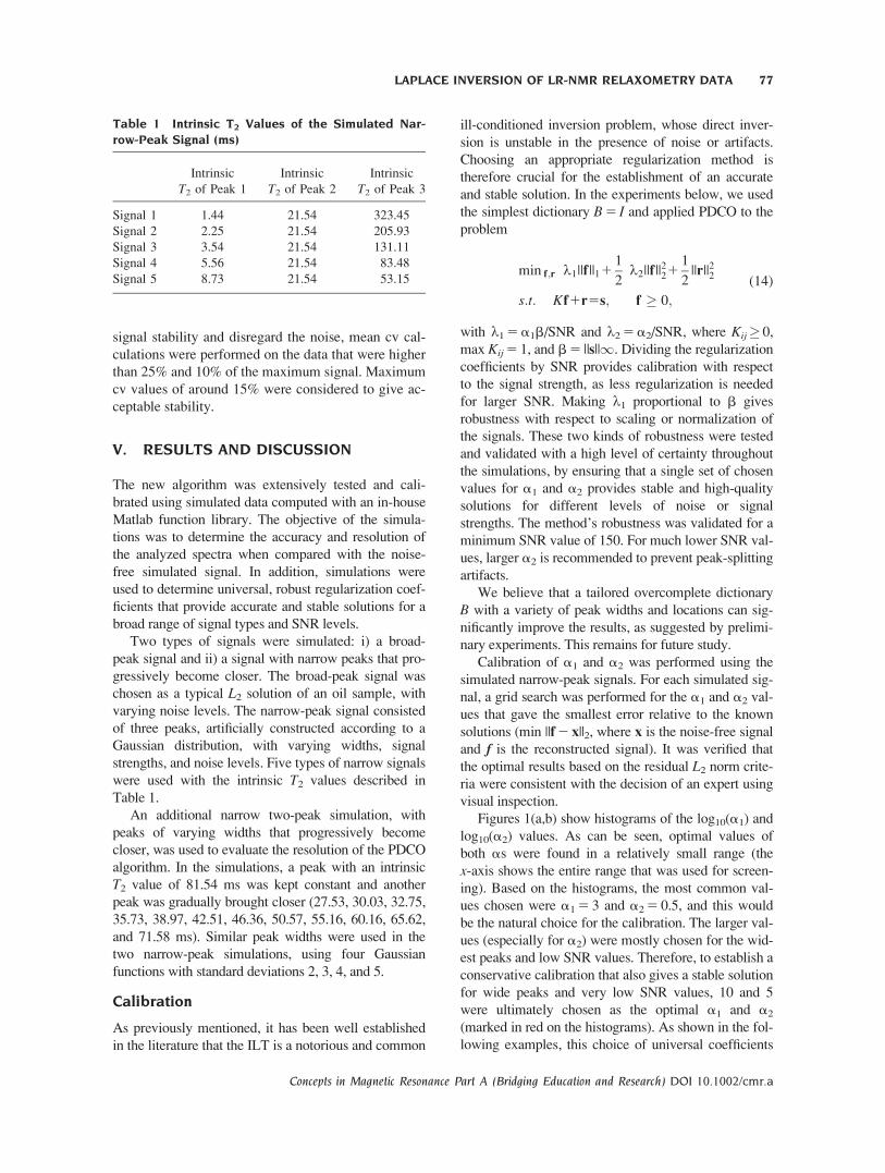
Two types of signals were simulated: i) a broad-

peak signal and ii) a signal with narrow peaks that pro-

gressively become closer. The broad-peak signal was

chosen as a typical L2 solution of an oil sample, with

varying noise levels. The narrow-peak signal consisted

of three peaks, artificially constructed according to a

Gaussian distribution, with varying widths, signal

strengths, and noise levels. Five types of narrow signals

were used with the intrinsic T2 values described in

Table 1.

An additional narrow two-peak simulation, with

peaks of varying widths that progressively become

closer, was used to evaluate the resolution of the PDCO

algorithm. In the simulations, a peak with an intrinsic

T2 value of 81.54 ms was kept constant and another

peak was gradually brought closer (27.53, 30.03, 32.75,

35.73, 38.97, 42.51, 46.36, 50.57, 55.16, 60.16, 65.62,

and 71.58 ms). Similar peak widths were used in the

two narrow-peak simulations, using four Gaussian

functions with standard deviations 2, 3, 4, and 5.

Calibration

As previously mentioned, it has been well established

in the literature that the ILT is a notorious and common

ill-conditioned inversion problem, whose direct inver-

sion is unstable in the presence of noise or artifacts.

Choosing an appropriate regularization method is

therefore crucial for the establishment of an accurate

and stable solution. In the experiments below, we used

the simplest dictionary B 5 I and applied PDCO to the

problem

min f;r k1||f ||111

2k2||f ||221

1

2||r||22

s:t: Kf1r5s; f � 0;

(14)

with k1 5 a1b/SNR and k2 5 a2/SNR, where Kij� 0,

max Kij 5 1, and b 5 ||s||1. Dividing the regularization

coefficients by SNR provides calibration with respect

to the signal strength, as less regularization is needed

for larger SNR. Making k1 proportional to b gives

robustness with respect to scaling or normalization of

the signals. These two kinds of robustness were tested

and validated with a high level of certainty throughout

the simulations, by ensuring that a single set of chosen

values for a1 and a2 provides stable and high-quality

solutions for different levels of noise or signal

strengths. The method’s robustness was validated for a

minimum SNR value of 150. For much lower SNR val-

ues, larger a2 is recommended to prevent peak-splitting

artifacts.

We believe that a tailored overcomplete dictionary

B with a variety of peak widths and locations can sig-

nificantly improve the results, as suggested by prelimi-

nary experiments. This remains for future study.

Calibration of a1 and a2 was performed using the

simulated narrow-peak signals. For each simulated sig-

nal, a grid search was performed for the a1 and a2 val-

ues that gave the smallest error relative to the known

solutions (min ||f 2 x||2, where x is the noise-free signal

and f is the reconstructed signal). It was verified that

the optimal results based on the residual L2 norm crite-

ria were consistent with the decision of an expert using

visual inspection.

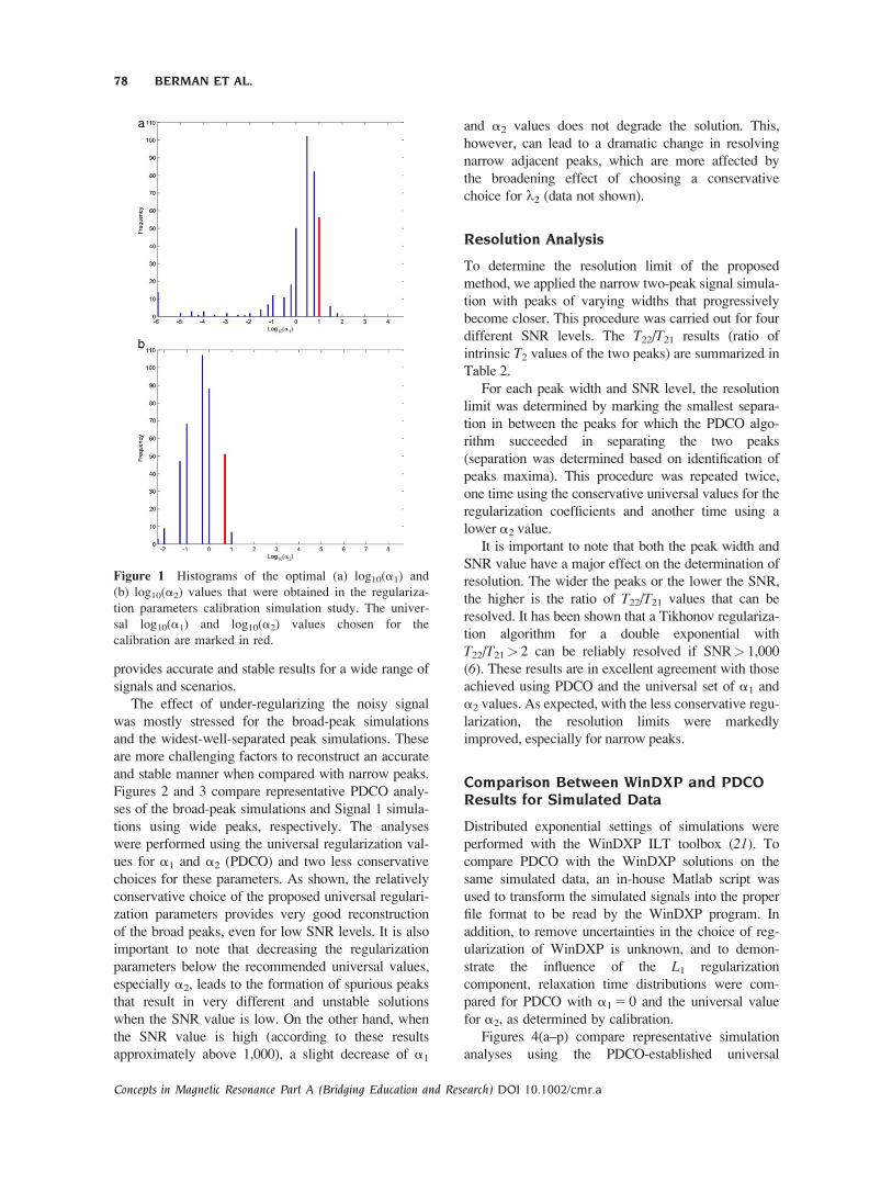
Figures 1(a,b) show histograms of the log10(a1) and

log10(a2) values. As can be seen, optimal values of

both as were found in a relatively small range (the

x-axis shows the entire range that was used for screen-

ing). Based on the histograms, the most common val-

ues chosen were a1 5 3 and a2 5 0.5, and this would

be the natural choice for the calibration. The larger val-

ues (especially for a2) were mostly chosen for the wid-

est peaks and low SNR values. Therefore, to establish a

conservative calibration that also gives a stable solution

for wide peaks and very low SNR values, 10 and 5

were ultimately chosen as the optimal a1 and a2

(marked in red on the histograms). As shown in the fol-

lowing examples, this choice of universal coefficients

Table 1 Intrinsic T2 Values of the Simulated Nar-row-Peak Signal (ms)

Intrinsic

T2 of Peak 1

Intrinsic

T2 of Peak 2

Intrinsic

T2 of Peak 3

Signal 1 1.44 21.54 323.45

Signal 2 2.25 21.54 205.93

Signal 3 3.54 21.54 131.11

Signal 4 5.56 21.54 83.48

Signal 5 8.73 21.54 53.15



provides accurate and stable results for a wide range of

signals and scenarios.

The effect of under-regularizing the noisy signal

was mostly stressed for the broad-peak simulations

and the widest-well-separated peak simulations. These

are more challenging factors to reconstruct an accurate

and stable manner when compared with narrow peaks.

Figures 2 and 3 compare representative PDCO analy-

ses of the broad-peak simulations and Signal 1 simula-

tions using wide peaks, respectively. The analyses

were performed using the universal regularization val-

ues for a1 and a2 (PDCO) and two less conservative

choices for these parameters. As shown, the relatively

conservative choice of the proposed universal regulari-

zation parameters provides very good reconstruction

of the broad peaks, even for low SNR levels. It is also

important to note that decreasing the regularization

parameters below the recommended universal values,

especially a2, leads to the formation of spurious peaks

that result in very different and unstable solutions

when the SNR value is low. On the other hand, when

the SNR value is high (according to these results

approximately above 1,000), a slight decrease of a1

and a2 values does not degrade the solution. This,

however, can lead to a dramatic change in resolving

narrow adjacent peaks, which are more affected by

the broadening effect of choosing a conservative

choice for k2 (data not shown).

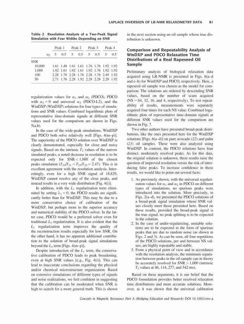
Resolution Analysis

To determine the resolution limit of the proposed

method, we applied the narrow two-peak signal simula-

tion with peaks of varying widths that progressively

become closer. This procedure was carried out for four

different SNR levels. The T22/T21 results (ratio of

intrinsic T2 values of the two peaks) are summarized in

Table 2.

For each peak width and SNR level, the resolution

limit was determined by marking the smallest separa-

tion in between the peaks for which the PDCO algo-

rithm succeeded in separating the two peaks

(separation was determined based on identification of

peaks maxima). This procedure was repeated twice,

one time using the conservative universal values for the

regularization coefficients and another time using a

lower a2 value.

It is important to note that both the peak width and

SNR value have a major effect on the determination of

resolution. The wider the peaks or the lower the SNR,

the higher is the ratio of T22/T21 values that can be

resolved. It has been shown that a Tikhonov regulariza-

tion algorithm for a double exponential with

T22/T21> 2 can be reliably resolved if SNR> 1,000

(6). These results are in excellent agreement with those

achieved using PDCO and the universal set of a1 and

a2 values. As expected, with the less conservative regu-

larization, the resolution limits were markedly

improved, especially for narrow peaks.

Comparison Between WinDXP and PDCOResults for Simulated Data

Distributed exponential settings of simulations were

performed with the WinDXP ILT toolbox (21). To

compare PDCO with the WinDXP solutions on the

same simulated data, an in-house Matlab script was

used to transform the simulated signals into the proper

file format to be read by the WinDXP program. In

addition, to remove uncertainties in the choice of reg-

ularization of WinDXP is unknown, and to demon-

strate the influence of the L1 regularization

component, relaxation time distributions were com-

pared for PDCO with a1 5 0 and the universal value

for a2, as determined by calibration.

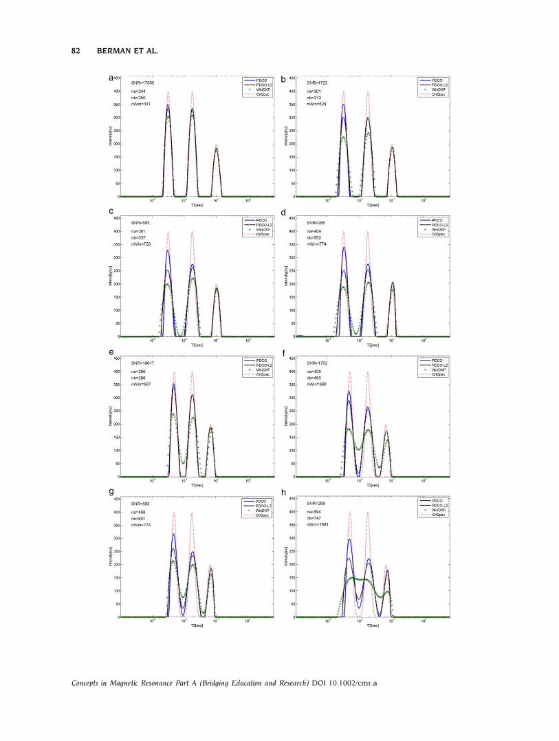
Figures 4(a–p) compare representative simulation

analyses using the PDCO-established universal

Figure 1 Histograms of the optimal (a) log10(a1) and

(b) log10(a2) values that were obtained in the regulariza-

tion parameters calibration simulation study. The univer-

sal log10(a1) and log10(a2) values chosen for the

calibration are marked in red.

78 BERMAN ET AL.


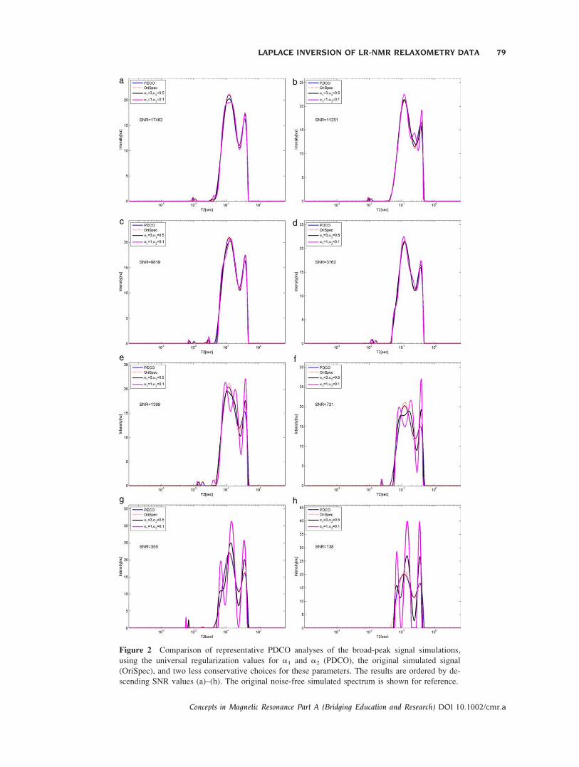
Figure 2 Comparison of representative PDCO analyses of the broad-peak signal simulations,

using the universal regularization values for a1 and a2 (PDCO), the original simulated signal

(OriSpec), and two less conservative choices for these parameters. The results are ordered by de-

scending SNR values (a)–(h). The original noise-free simulated spectrum is shown for reference.



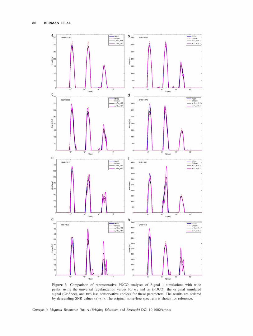
Figure 3 Comparison of representative PDCO analyses of Signal 1 simulations with wide

peaks, using the universal regularization values for a1 and a2 (PDCO), the original simulated

signal (OriSpec), and two less conservative choices for these parameters. The results are ordered

by descending SNR values (a)–(h). The original noise-free spectrum is shown for reference.

80 BERMAN ET AL.


regularization values for a1 and a2 (PDCO), PDCO

with a1 5 0 and universal a2 (PDCO-L2), and the

WinDXP (WinDXP) solutions for four types of simula-

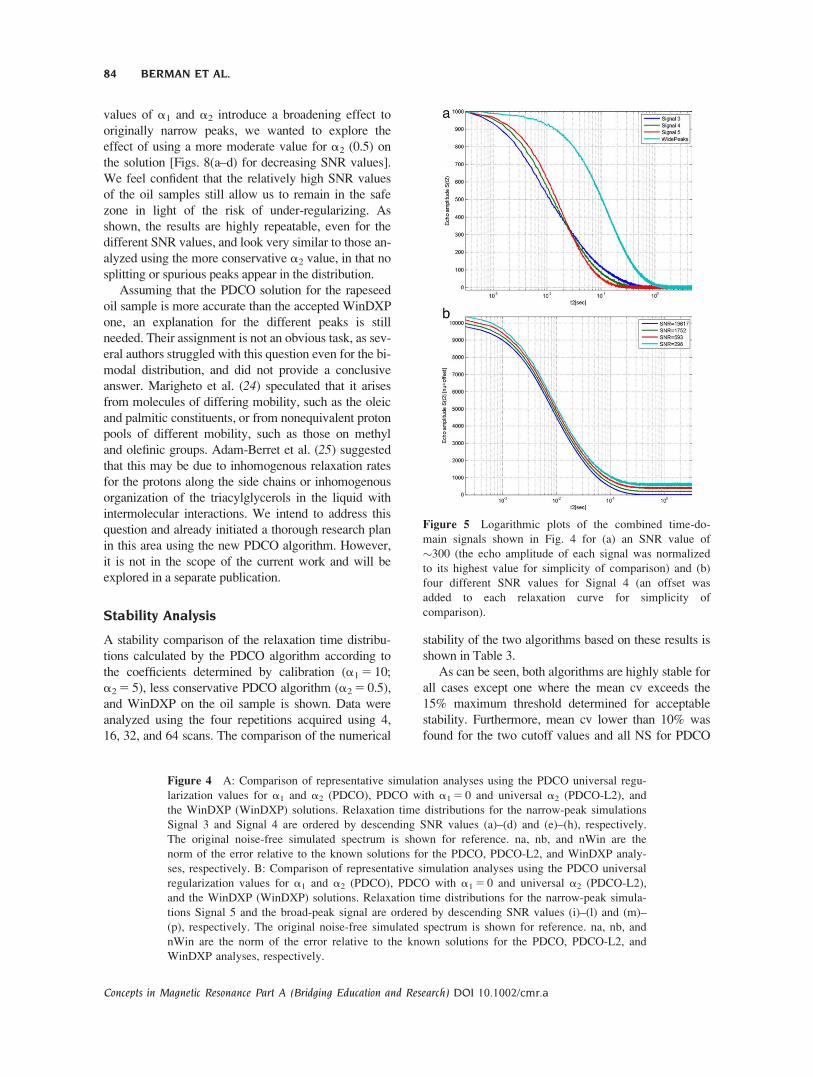
tions and SNR values. Combined logarithmic plots of

representative time-domain signals at different SNR

values used for the comparison are shown in Figs.

5(a,b).

In the case of the wide-peak simulations, WinDXP

and PDCO both solve relatively well [Figs. 4(m–p)].

The superiority of the PDCO solution over WinDXP is

clearly demonstrated, especially for close and noisy

signals. Based on the intrinsic T2 values of the narrow

simulated peaks, a noted decrease in resolution is to be

expected only for SNR< 1,000 of the closest

peaks simulation (T22/T21 5 T23/T22 5 2.47). This is in

excellent agreement with the resolution analysis. Inter-

estingly, even for a high SNR signal of 18,829,

WinDXP cannot resolve any of the close peaks, and

instead results in a very wide distribution [Fig. 4(i)].

In addition, with the L1 regularization term elimi-

nated by setting k1 5 0, the PDCO results are signifi-

cantly better than for WinDXP. This may be due to a

more conservative choice of calibration of the

WinDXP, but perhaps more to the superior accuracy

and numerical stability of the PDCO solver. In the lat-

ter case, PDCO would be a preferred solver even for

traditional L2 regularization. It is also evident that the

L1 regularization term improves the quality of

the reconstruction results especially for low SNR. On

the other hand, it has no apparent additional contribu-

tion to the solution of broad-peak signal simulations

beyond the L2 term [Figs. 4(m–p)].

Despite introduction of the L1 term, the conserva-

tive calibration of PDCO leads to peak broadening,

even at high SNR values [e.g., Fig. 4(i)]. This can

lead to inaccurate conclusions regarding the physical

and/or chemical microstructure organization. Based

on extensive simulations of different types of signals

and noise realizations, we feel confident in suggesting

that the calibration can be moderated when SNR is

high to search for a more general truth. This is shown

in the next section using an oil sample whose true dis-

tribution is unknown.

Comparison and Repeatability Analysis ofWinDXP and PDCO Relaxation TimeDistributions of a Real Rapeseed OilSample

Preliminary analysis of biological relaxation data

acquired using LR-NMR is presented in Figs. 6(a–d

and e–h) for WinDXP and PDCO, respectively. Here, a

rapeseed oil sample was chosen as the model for com-

parison. The solutions are ordered by descending SNR

values, based on the number of scans acquired

(NS 5 64, 32, 16, and 4, respectively). To test repeat-

ability of results, measurements were separately

acquired four times for each NS value. Combined loga-

rithmic plots of representative time-domain signals at

different SNR values used for the comparison are

shown in Fig. 7.

Two other authors have presented broad-peak distri-

butions, like the ones presented here for the WinDXP

solutions [Figs. 6(a–d)] on pure avocado (22) and palm

(23) oil samples. These were also analyzed using

WinDXP. In contrast, the PDCO solutions have four

distinct, moderately resolved peaks. As for this data,

the original solution is unknown, these results raise the

question of improved resolution versus the risk of intro-

ducing false peaks. To increase confidence in these

results, we would like to point out several facts:

1. As previously shown, with the universal regulari-zation values for a1 and a2 in PDCO on differenttypes of simulations, no spurious peaks wereintroduced into the solution. More precisely, inFigs. 2(a–d), we presented the PDCO solutions ofa broad-peak signal simulation whose SNR val-ues closely meet those presented here. Based onthese results, provided the broad-peak signal isthe true signal, no peak splitting is to be expectedin the solution.

2. In the case of under-regularizing, unstable solu-tions are to be expected in the form of spuriouspeaks that are due to random noise (as shown inFigs. 2 and 3). As can be seen, all four repetitionsof the PDCO solutions, per and between NS val-ues, are highly repeatable and stable.

3. From a physical point of view and in accordancewith the resolution analysis, the minimum separa-tion between peaks in the oil sample can in theorybe accurately resolved for SNR> 1,000 (intrinsicT2 values at 46, 114, 277, and 542 ms).

Based on these arguments, it is our belief that the

PDCO formulation provides better resolved relaxation

time distributions and more accurate solutions. More-

over, as it was shown that the universal calibration

Table 2 Resolution Analysis of a Two-Peak SignalSimulation with Four Widths Depending on SNR

Peak 1 Peak 2 Peak 3 Peak 4

a2 5 0.5 5 0.5 5 0.5 5 0.5

SNR

10,000 1.61 1.48 1.61 1.61 1.76 1.76 1.92 1.92

1,000 1.92 1.61 1.92 1.61 1.92 1.76 1.92 1.92

100 2.28 1.76 2.28 1.76 2.28 1.76 2.49 1.92

50 2.71 1.76 2.28 1.92 2.28 2.28 2.28 1.92



82 BERMAN ET AL.


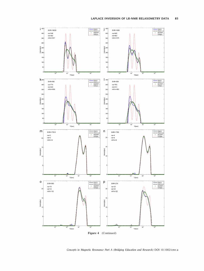
Figure 4 (Continued)



values of a1 and a2 introduce a broadening effect to

originally narrow peaks, we wanted to explore the

effect of using a more moderate value for a2 (0.5) on

the solution [Figs. 8(a–d) for decreasing SNR values].

We feel confident that the relatively high SNR values

of the oil samples still allow us to remain in the safe

zone in light of the risk of under-regularizing. As

shown, the results are highly repeatable, even for the

different SNR values, and look very similar to those an-

alyzed using the more conservative a2 value, in that no

splitting or spurious peaks appear in the distribution.

Assuming that the PDCO solution for the rapeseed

oil sample is more accurate than the accepted WinDXP

one, an explanation for the different peaks is still

needed. Their assignment is not an obvious task, as sev-

eral authors struggled with this question even for the bi-

modal distribution, and did not provide a conclusive

answer. Marigheto et al. (24) speculated that it arises

from molecules of differing mobility, such as the oleic

and palmitic constituents, or from nonequivalent proton

pools of different mobility, such as those on methyl

and olefinic groups. Adam-Berret et al. (25) suggested

that this may be due to inhomogenous relaxation rates

for the protons along the side chains or inhomogenous

organization of the triacylglycerols in the liquid with

intermolecular interactions. We intend to address this

question and already initiated a thorough research plan

in this area using the new PDCO algorithm. However,

it is not in the scope of the current work and will be

explored in a separate publication.

Stability Analysis

A stability comparison of the relaxation time distribu-

tions calculated by the PDCO algorithm according to

the coefficients determined by calibration (a1 5 10;

a2 5 5), less conservative PDCO algorithm (a2 5 0.5),

and WinDXP on the oil sample is shown. Data were

analyzed using the four repetitions acquired using 4,

16, 32, and 64 scans. The comparison of the numerical

stability of the two algorithms based on these results is

shown in Table 3.

As can be seen, both algorithms are highly stable for

all cases except one where the mean cv exceeds the

15% maximum threshold determined for acceptable

stability. Furthermore, mean cv lower than 10% was

found for the two cutoff values and all NS for PDCO

Figure 4 A: Comparison of representative simulation analyses using the PDCO universal regu-

larization values for a1 and a2 (PDCO), PDCO with a1 5 0 and universal a2 (PDCO-L2), and

the WinDXP (WinDXP) solutions. Relaxation time distributions for the narrow-peak simulations

Signal 3 and Signal 4 are ordered by descending SNR values (a)–(d) and (e)–(h), respectively.

The original noise-free simulated spectrum is shown for reference. na, nb, and nWin are the

norm of the error relative to the known solutions for the PDCO, PDCO-L2, and WinDXP analy-

ses, respectively. B: Comparison of representative simulation analyses using the PDCO universal

regularization values for a1 and a2 (PDCO), PDCO with a1 5 0 and universal a2 (PDCO-L2),

and the WinDXP (WinDXP) solutions. Relaxation time distributions for the narrow-peak simula-

tions Signal 5 and the broad-peak signal are ordered by descending SNR values (i)–(l) and (m)–

(p), respectively. The original noise-free simulated spectrum is shown for reference. na, nb, and

nWin are the norm of the error relative to the known solutions for the PDCO, PDCO-L2, and

WinDXP analyses, respectively.

Figure 5 Logarithmic plots of the combined time-do-

main signals shown in Fig. 4 for (a) an SNR value of

�300 (the echo amplitude of each signal was normalized

to its highest value for simplicity of comparison) and (b)

four different SNR values for Signal 4 (an offset was

added to each relaxation curve for simplicity of

comparison).

84 BERMAN ET AL.


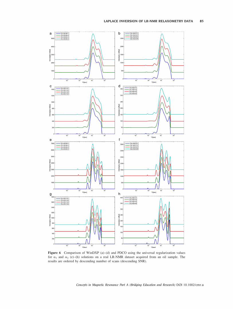
Figure 6 Comparison of WinDXP (a)–(d) and PDCO using the universal regularization values

for a1 and a2 (e)–(h) solutions on a real LR-NMR dataset acquired from an oil sample. The

results are ordered by descending number of scans (descending SNR).



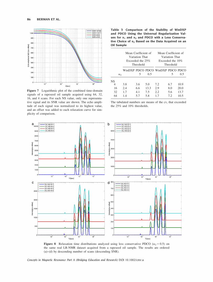
Figure 7 Logarithmic plot of the combined time-domain

signals of a rapeseed oil sample acquired using 64, 32,

16, and 4 scans. For each NS value, only one representa-

tive signal and its SNR value are shown. The echo ampli-

tude of each signal was normalized to its highest value,

and an offset was added to each relaxation curve for sim-

plicity of comparison.

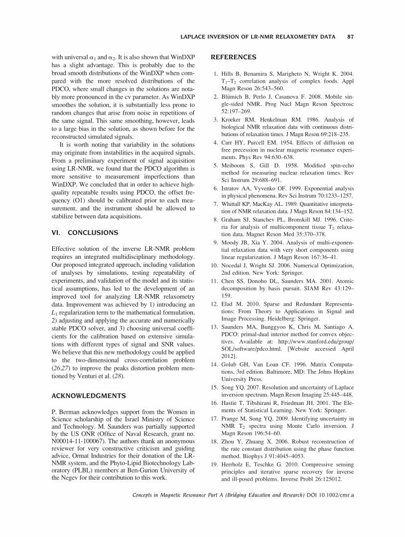
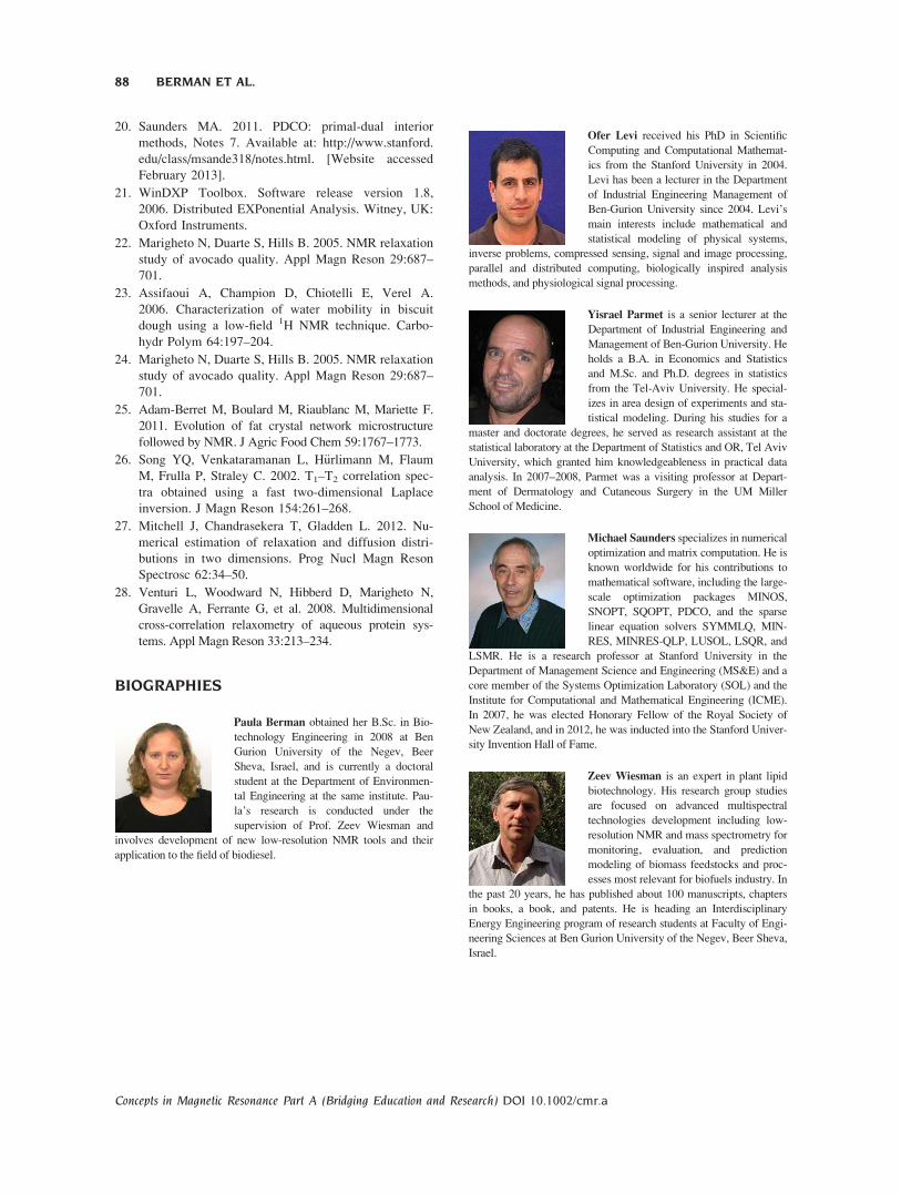
Figure 8 Relaxation time distributions analyzed using less conservative PDCO (a2 5 0.5) on

the same real LR-NMR dataset acquired from a rapeseed oil sample. The results are ordered

(a)–(d) by descending number of scans (descending SNR).

Table 3 Comparison of the Stability of WinDXPand PDCO Using the Universal Regularization Val-ues for a1 and a2 and PDCO with a Less Conserva-

tive Choice of a2 Based on the Data Acquired on anOil Sample

Mean Coefficient of

Variation That

Exceeded the 25%

Threshold

Mean Coefficient of

Variation That

Exceeded the 10%

Threshold

WinDXP PDCO PDCO WinDXP PDCO PDCO

a2 5 0.5 5 0.5

NS4 3.8 3.6 5.0 7.2 6.7 10.9

16 2.4 6.6 13.3 2.9 8.0 20.0

32 1.7 4.1 7.5 2.2 5.6 13.7

64 1.4 5.7 5.8 1.7 7.2 10.5

The tabulated numbers are means of the cvi that exceeded

the 25% and 10% thresholds.

86 BERMAN ET AL.


with universal a1 and a2. It is also shown that WinDXP

has a slight advantage. This is probably due to the

broad smooth distributions of the WinDXP when com-

pared with the more resolved distributions of the

PDCO, where small changes in the solutions are nota-

bly more pronounced in the cv parameter. As WinDXP

smoothes the solution, it is substantially less prone to

random changes that arise from noise in repetitions of

the same signal. This same smoothing, however, leads

to a large bias in the solution, as shown before for the

reconstructed simulated signals.

It is worth noting that variability in the solutions

may originate from instabilities in the acquired signals.

From a preliminary experiment of signal acquisition

using LR-NMR, we found that the PDCO algorithm is

more sensitive to measurement imperfections than

WinDXP. We concluded that in order to achieve high-

quality repeatable results using PDCO, the offset fre-

quency (O1) should be calibrated prior to each mea-

surement, and the instrument should be allowed to

stabilize between data acquisitions.

VI. CONCLUSIONS

Effective solution of the inverse LR-NMR problem

requires an integrated multidisciplinary methodology.

Our proposed integrated approach, including validation

of analyses by simulations, testing repeatability of

experiments, and validation of the model and its statis-

tical assumptions, has led to the development of an

improved tool for analyzing LR-NMR relaxometry

data. Improvement was achieved by 1) introducing an

L1 regularization term to the mathematical formulation,

2) adjusting and applying the accurate and numerically

stable PDCO solver, and 3) choosing universal coeffi-

cients for the calibration based on extensive simula-

tions with different types of signal and SNR values.

We believe that this new methodology could be applied

to the two-dimensional cross-correlation problem

(26,27) to improve the peaks distortion problem men-

tioned by Venturi et al. (28).

ACKNOWLEDGMENTS

P. Berman acknowledges support from the Women inScience scholarship of the Israel Ministry of Scienceand Technology. M. Saunders was partially supportedby the US ONR (Office of Naval Research, grant no.N00014-11-100067). The authors thank an anonymousreviewer for very constructive criticism and guidingadvice, Ormat Industries for their donation of the LR-NMR system, and the Phyto-Lipid Biotechnology Lab-oratory (PLBL) members at Ben-Gurion University ofthe Negev for their contribution to this work.

REFERENCES

1. Hills B, Benamira S, Marigheto N, Wright K. 2004.

T1–T2 correlation analysis of complex foods. Appl

Magn Reson 26:543–560.

2. Bl€umich B, Perlo J, Casanova F. 2008. Mobile sin-

gle-sided NMR. Prog Nucl Magn Reson Spectrosc

52:197–269.

3. Kroeker RM, Henkelman RM. 1986. Analysis of

biological NMR relaxation data with continuous distri-

butions of relaxation times. J Magn Reson 69:218–235.

4. Carr HY, Purcell EM. 1954. Effects of diffusion on

free precession in nuclear magnetic resonance experi-

ments. Phys Rev 94:630–638.

5. Meiboom S, Gill D. 1958. Modified spin-echo

method for measuring nuclear relaxation times. Rev

Sci Instrum 29:688–691.

6. Istratov AA, Vyvenko OF. 1999. Exponential analysis

in physical phenomena. Rev Sci Instrum 70:1233–1257.

7. Whittall KP, MacKay AL. 1989. Quantitative interpreta-

tion of NMR relaxation data. J Magn Reson 84:134–152.

8. Graham SJ, Stanchev PL, Bronskill MJ. 1996. Crite-

ria for analysis of multicomponent tissue T2 relaxa-

tion data. Magnet Reson Med 35:370–378.

9. Moody JB, Xia Y. 2004. Analysis of multi-exponen-

tial relaxation data with very short components using

linear regularization. J Magn Reson 167:36–41.

10. Nocedal J, Wright SJ. 2006. Numerical Optimization,

2nd edition. New York: Springer.

11. Chen SS, Donoho DL, Saunders MA. 2001. Atomic

decomposition by basis pursuit. SIAM Rev 43:129–

159.

12. Elad M. 2010. Sparse and Redundant Representa-

tions: From Theory to Applications in Signal and

Image Processing. Heidelberg: Springer.

13. Saunders MA, Bunggyoo K, Chris M, Santiago A.

PDCO: primal-dual interior method for convex objec-

tives. Available at: http://www.stanford.edu/group/

SOL/software/pdco.html. [Website accessed April

2012].

14. Golub GH, Van Loan CF. 1996. Matrix Computa-

tions, 3rd edition. Baltimore, MD: The Johns Hopkins

University Press.

15. Song YQ. 2007. Resolution and uncertainty of Laplace

inversion spectrum. Magn Reson Imaging 25:445–448.

16. Hastie T, Tibshirani R, Friedman JH. 2001. The Ele-

ments of Statistical Learning. New York: Springer.

17. Prange M, Song YQ. 2009. Identifying uncertainty in

NMR T2 spectra using Monte Carlo inversion. J

Magn Reson 196:54–60.

18. Zhou Y, Zhuang X. 2006. Robust reconstruction of

the rate constant distribution using the phase function

method. Biophys J 91:4045–4053.

19. Herrholz E, Teschke G. 2010. Compressive sensing

principles and iterative sparse recovery for inverse

and ill-posed problems. Inverse Probl 26:125012.



20. Saunders MA. 2011. PDCO: primal-dual interior

methods, Notes 7. Available at: http://www.stanford.

edu/class/msande318/notes.html. [Website accessed

February 2013].

21. WinDXP Toolbox. Software release version 1.8,

2006. Distributed EXPonential Analysis. Witney, UK:

Oxford Instruments.

22. Marigheto N, Duarte S, Hills B. 2005. NMR relaxation

study of avocado quality. Appl Magn Reson 29:687–

701.

23. Assifaoui A, Champion D, Chiotelli E, Verel A.

2006. Characterization of water mobility in biscuit

dough using a low-field 1H NMR technique. Carbo-

hydr Polym 64:197–204.

24. Marigheto N, Duarte S, Hills B. 2005. NMR relaxation

study of avocado quality. Appl Magn Reson 29:687–

701.

25. Adam-Berret M, Boulard M, Riaublanc M, Mariette F.

2011. Evolution of fat crystal network microstructure

followed by NMR. J Agric Food Chem 59:1767–1773.

26. Song YQ, Venkataramanan L, H€urlimann M, Flaum

M, Frulla P, Straley C. 2002. T1–T2 correlation spec-

tra obtained using a fast two-dimensional Laplace

inversion. J Magn Reson 154:261–268.

27. Mitchell J, Chandrasekera T, Gladden L. 2012. Nu-

merical estimation of relaxation and diffusion distri-

butions in two dimensions. Prog Nucl Magn Reson

Spectrosc 62:34–50.

28. Venturi L, Woodward N, Hibberd D, Marigheto N,

Gravelle A, Ferrante G, et al. 2008. Multidimensional

cross-correlation relaxometry of aqueous protein sys-

tems. Appl Magn Reson 33:213–234.

BIOGRAPHIES

Paula Berman obtained her B.Sc. in Bio-

technology Engineering in 2008 at Ben

Gurion University of the Negev, Beer

Sheva, Israel, and is currently a doctoral

student at the Department of Environmen-

tal Engineering at the same institute. Pau-

la’s research is conducted under the

supervision of Prof. Zeev Wiesman and

involves development of new low-resolution NMR tools and their

application to the field of biodiesel.

Ofer Levi received his PhD in Scientific

Computing and Computational Mathemat-

ics from the Stanford University in 2004.

Levi has been a lecturer in the Department

of Industrial Engineering Management of

Ben-Gurion University since 2004. Levi’s

main interests include mathematical and

statistical modeling of physical systems,

inverse problems, compressed sensing, signal and image processing,

parallel and distributed computing, biologically inspired analysis

methods, and physiological signal processing.

Yisrael Parmet is a senior lecturer at the

Department of Industrial Engineering and

Management of Ben-Gurion University. He

holds a B.A. in Economics and Statistics

and M.Sc. and Ph.D. degrees in statistics

from the Tel-Aviv University. He special-

izes in area design of experiments and sta-

tistical modeling. During his studies for a

master and doctorate degrees, he served as research assistant at the

statistical laboratory at the Department of Statistics and OR, Tel Aviv

University, which granted him knowledgeableness in practical data

analysis. In 2007–2008, Parmet was a visiting professor at Depart-

ment of Dermatology and Cutaneous Surgery in the UM Miller

School of Medicine.

Michael Saunders specializes in numerical

optimization and matrix computation. He is

known worldwide for his contributions to

mathematical software, including the large-

scale optimization packages MINOS,

SNOPT, SQOPT, PDCO, and the sparse

linear equation solvers SYMMLQ, MIN-

RES, MINRES-QLP, LUSOL, LSQR, and

LSMR. He is a research professor at Stanford University in the

Department of Management Science and Engineering (MS&E) and a

core member of the Systems Optimization Laboratory (SOL) and the

Institute for Computational and Mathematical Engineering (ICME).

In 2007, he was elected Honorary Fellow of the Royal Society of

New Zealand, and in 2012, he was inducted into the Stanford Univer-

sity Invention Hall of Fame.

Zeev Wiesman is an expert in plant lipid

biotechnology. His research group studies

are focused on advanced multispectral

technologies development including low-

resolution NMR and mass spectrometry for

monitoring, evaluation, and prediction

modeling of biomass feedstocks and proc-

esses most relevant for biofuels industry. In

the past 20 years, he has published about 100 manuscripts, chapters

in books, a book, and patents. He is heading an Interdisciplinary

Energy Engineering program of research students at Faculty of Engi-

neering Sciences at Ben Gurion University of the Negev, Beer Sheva,

Israel.

88 BERMAN ET AL.


Documents

Laplace Inversion of Low-Resolution NMR Relaxometry …web.stanford.edu/group/SOL/papers/CMR21263.pdf · Laplace Inversion of ... Relaxometry Data Using Sparse Representation Methods