Large Deviations and the Distribution of Price Changes

Laurent Calvet and Adlai Fisher∗

Department of Economics, Yale University

Benoit Mandelbrot†

Department of Mathematics, Yale University andIBM T. J. Watson Research Center

Cowles Foundation Discussion Paper No. 1165

This Draft: September 15, 1997First Draft: October 1996

∗28 Hillhouse Avenue, New Haven, CT 06520-1972. e-mail: lcalvet@minerva.cis.yale.edu, fisher@econ.yale.edu†10 Hillhouse Avenue, New Haven, CT 06520-8283. e-mail: fractal@watson.ibm.com

Abstract

The Multifractal Model of Asset Returns (“MMAR”, See Mandelbrot, Fisher, and Cal-

vet, 1997) proposes a class of multifractal processes for the modelling of financial returns.

In that paper, multifractal processes are defined by a scaling law for moments of the

processes’ increments over finite time intervals. In the present paper, we discuss the

local behavior of multifractal processes. We employ local Holder exponents, a funda-

mental concept in real analysis that describes the local scaling properties of a realized

path at any point in time. In contrast with the standard models of continuous time

finance, multifractal processes contain a multiplicity of local Holder exponents within

any finite time interval. We characterize the distribution of Holder exponents by the

multifractal spectrum of the process. For a broad class of multifractal processes, this

distribution can be obtained by an application of Cramer’s Large Deviation Theory. In

an alternative interpretation, the multifractal spectrum describes the fractal dimension

of the set of points having a given local Holder exponent. Finally, we show how to

obtain processes with varied spectra. This allows the applied researcher to relate an

empirical estimate of the multifractal spectrum back to a particular construction of the

stochastic process.

Keywords: Multifractal Model of Asset Returns, Multifractal Spectrum, Compound

Stochastic Process, Subordinated Stochastic Process, Time Deformation, Scaling Laws,

Self-Similarity, Self-Affinity

1 Introduction

The Multifractal Model of Asset Returns (MMAR) proposes a class of multifractal processes for the

modelling of financial prices. In Mandelbrot, Fisher and Calvet (1997), multifractality is defined

by the scaling properties of the processes’ moments over different time increments. This “global”

definition imposes restrictions on the unconditional distributions of the price process. It pays little

attention however to the heterogeneity of price variability across time, which has recently attracted

much attention from econometricians.

In this paper, we focus on the “local” behavior of the MMAR. Our approach is based on the

local Holder exponent, a fundamental concept in real analysis that describes the scaling properties

of a realized path at any point in time. This concept can be heuristically defined as follows. On a

fixed realized path, the infinitesimal variation in price around a date t is of the form:

|P (t+ dt) − P (t)| ∼ Ct(dt)α(t),

where α(t) and Ct are respectively called the local Holder exponent and the prefactor at t.

In typical financial models, the local Holder exponent can only take a finite number of values.

For instance continuous Ito processes have the property that α(t) = 1/2 everywhere. Much recent

research on these processes has attempted to model the time-varying volatility, i.e. the prefactor

Ct. A good presentation of these advances is contained in Rossi (1997). Financial economists have

also used long memory processes based on the Fractional Brownian Motion (FBM) of Mandelbrot

and Van Ness (1968). The FBM contains a single local Holder exponent, its index of self-affinity.

Discontinuities or jumps have sometimes been added to these models, and permit local Holder

exponents equal to zero. In short, these traditional financial models contain at most two Holder

exponents along their sample paths.

There is however little justification for this choice, since temporal heterogeneity can be caused

by variations in both the local Holder exponent and the prefactor. We show in this paper that

the MMAR captures this possibility and contains a continuum of local Holder exponents. Their

distribution can be represented by a renormalized density called the multifractal spectrum. In

an alternative interpretation, the spectrum describes the fractal dimension of the set of instants

having a given local exponent. The statistical self-similarity of these sets accounts for long memory

in the process. For a broad class of multifractals, this distribution is obtained by an application of

1

Cramer’s Large Deviation Theory. We derive closed-form expressions for the spectra of particular

processes. This allows the applied researcher to relate an empirical estimate of the multifractal

spectrum back to a particular construction of the stochastic process.

Section 2 presents a brief review of multifractal measures and processes. Section 3 defines

the concept of multifractal spectrum. Section 4 introduces Cramer’s Large Deviation Theory and

derives the spectrum for a large class of multifractals. Section 5 applies these ideas to the MMAR.

Section 6 concludes.

2 Multifractals

This section presents a brief review of multifractal measures and processes. A more detailed dis-

cussion of these topics can be found in the companion theoretical paper, Mandelbrot, Fisher and

Calvet (1997).

2.1 The Binomial Measure

This section introduces the simplest multifractal, the binomial measure1 on the compact interval

[0, 1]. This is the limit of an elementary iterative procedure called a multiplicative cascade.

Letm0 andm1 be two positive numbers adding up to 1. At stage k = 0, we start the construction

with the uniform probability measure µ0 on [0, 1]. In the step k = 1, the measure µ1 uniformly

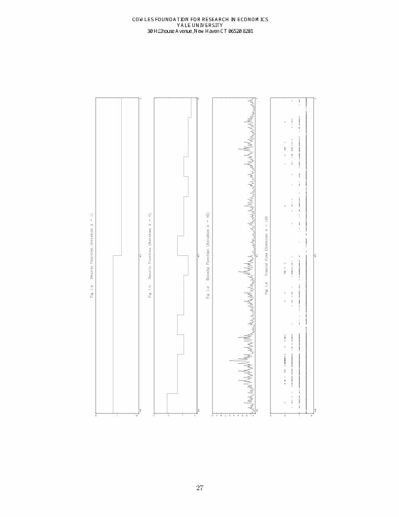
spreads mass equal to m0 on the subinterval [0, 1/2] and mass equal to m1 on [1/2, 1]. Figure 1a

represents the density of µ1 when m0 = 0.6.

In step k = 2, the set [0, 1/2] is split into two subintervals, [0, 1/4] and [1/4, 1/2], which respec-

tively receive a fraction m0 and m1 of the initial mass µ1[0, 1/2]. We apply the same procedure to

the dyadic set [1/2, 1] and obtain:

µ2[0, 1/4] = m0m0, µ2[1/4, 1/2] = m0m1,

µ2[1/2, 3/4] = m1m0, µ2[3/4, 1] = m1m1.

An infinite repetition of this scheme generates a sequence of measures (µk) that converges to the

binomial measure µ. Figure 1b represents the measure µ4 obtained after k = 4 steps.

The properties of the binomial are now briefly reviewed. Consider the dyadic interval [t, t+2−k],

1The binomial measure is sometimes called the Bernoulli or Besicovitch measure.

2

where

t = 0.η1η2..ηk =k∑

i=1

ηi2−i

in the counting base b = 2. Let ϕ0 and ϕ1 denote the relative frequencies of 0’s and 1’s in the

binary development of t. The measure of the dyadic interval simplifies to:

µ[t, t+ 2−k] = mkϕ00 mkϕ1

1 .

The binomial measure has important characteristics common to many multifractals. It is a con-

tinuous but singular probability measure. The procedure preserves at each stage the mass of split

dyadic intervals and is accordingly called conservative or microcanonical.

This construction can receive several extensions. For instance at each stage of the cascade,

intervals can be split not in 2 but in b > 2 intervals of equal size. Subintervals, indexed from left

to right by β (0 ≤ β ≤ b− 1), receive fractions of the total mass equal to m0, ..,mb−1. In order to

conserve mass these fractions, also called multipliers, are restricted to add up to one:∑mβ = 1.

This defines the class of multinomial measures, which are discussed in Mandelbrot (1989a) and

Evertsz and Mandelbrot (1992).

In another extension, the allocation of mass in the cascade becomes random. The multiplier of

each subinterval is a discrete random variable Mβ that takes values m0,m1, ...,mb−1 with proba-

bilities p0, .., pb−1. The preservation of mass imposes the additivity constraint:∑Mβ = 1. Figure

1c shows the random density obtained after k = 10 iterations with parameters b = 2, p = p0 = 0.5

and m0 = 0.6.

2.2 Multiplicative Measures

Multiplicative measures generalize the previous constructions by allowing multipliers Mβ (0 ≤ β ≤

b−1) that are not necessarily discrete, but may be more general random variables. To simplify the

presentation, we assume that the multipliers Mβ are identically distributed.

We first assume that mass is preserved at every stage of the construction:∑Mβ = 1. The

resulting measure is then called microcanonical or micro-conservative. Given a date t = 0.η1...ηk

and a length ∆t = b−k, the measure µ(∆t) of the b-adic cell [t, t+ ∆t] satisfies:

µ(∆t) = M(η1)M(η1, η2)...M(η1, ..., ηk).

3

Since multipliers at different stages of the cascade are independent, the moments of the measure

are of the form: E [µ(∆t)q] = [E(M q)]k for all admissible q ≥ 0. With the notation τ(q) =

− logb E(M q) − 1, this expression can be rewritten:

E [µ(∆t)q] = (∆t)τ(q)+1.

The measure thus satisfies the scaling property characterizing multifractals.2

Modifying the previous construction, we now choose that the multipliers Mβ be statistically

independent. Each iteration only conserves mass “on average” in the sense that E (∑Mβ) = 1

or EM = 1/b. The corresponding measure is then called canonical or canonical. Its total mass,

denoted Ω, is generally random3, and the mass of a b-adic cell takes the form:

µ(∆t) = Ω(η1, ..., ηk)M(η1)M(η1, η2)...M(η1, ..., ηk).

We note that Ω(η1, ..., ηk) has the same distribution as Ω. The measure thus satisfies the scaling

relationship:

E [µ(∆t)q] = E (Ωq) (∆t)τ(q)+1,

which characterizes multifractals.

2.3 Multifractal Processes

The concept of multifractality easily extends to stochastic processes.

Definition 1 A stochastic process X(t) is called multifractal if it satisfies:

E (|X(t)|q) = c(q)tτ(q)+1, for all t ∈ T , q ∈ Q, (1)

where T and Q are intervals on the real line, and τ(q) and c(q) are functions with domain Q.Moreover, we assume that T and Q have positive lengths, and that 0 ∈ T , [0, 1] ⊆ Q.

The function τ(q) is called the scaling function of the multifractal process. It is concave and

has intercept τ(0) = −1. Multifractals are called uniscaling when τ(q) is linear, and multiscaling

otherwise. We now justify this terminology and show in which sense multiscaling processes have a

multiplicity of local scales.

2To simplify exposition, we directly define multifractals via this property. For a more rigorous treatment, whichbegins by defining multifractals as statistically self-similar measures, and develops their properties, see Mandelbrot(1989a).

3The random variable Ω has interesting distributional and tail properties that are discussed in Mandelbrot (1989a).

4

3 Local Holder Exponents and the Multifractal Spectrum

3.1 Local Holder Exponent

We first introduce a concept borrowed from real analysis which characterizes the smoothness of a

function at a given date.

Definition 2 Let g be a function defined on the neighborhood of a given date t. The number

α(t) = Sup β ≥ 0 : |g(t+ 4t) − g(t)| = O(|4t|β) as 4t→ 0

is called the Holder exponent of g at t.

The Holder exponent is sometimes called the “local strength of singularity.” It always exists

and is generally valued in [−∞,+∞]. We note that α(t) is non-negative if (and only if) the function

g is bounded around t. For simplicity, this paper only considers functions locally bounded on their

domains, which guarantees the non-negativity of all Holder exponents.

Definition 3.1 readily extends to measures defined on the real line. At a given date t, the local

exponent of a measure is simply defined as the local exponent of its c.d.f. Since measures are

bounded, the Holder exponents are everywhere non-negative.

The Holder exponent receives an intuitive interpretation when the infinitesimal variations of

the function satisfy the scaling relationship4:

|g(t+ 4t) − g(t)| ∼ Ct(4t)α(t), (2)

where the positive constant Ct is called prefactor. The local Holder exponent then appears as a

local scale in the sense of fractal geometry. This approach to Holder exponents is further discussed

in Mandelbrot (1982, pp. 373-374).

From equation (2), we can easily compute the exponents of several examples. For instance the

local scale is 0 at points of discontinuity, and 1 at differentiable points where g′ 6= 0. The Holder

exponents of elementary functions are thus integers almost everywhere (a.e.). Non integer exponents

appear with greater frequency in very winding continuous functions. For instance the jagged paths

of Brownian motions are characterized by Holder exponents equal to 1/2. This property holds in

fact for all continuous Ito processes. Fractional Brownian Motions BH(t) also have a unique Holder

exponent, their index of self-affinity H. By contrast, the next section shows that multifractals

contain a multiplicity of local scales.4The expression (∆t)α(t) is an example of “non-standard infinitesimal”, as developed by Abraham Robinson.

5

3.2 The Multifractal Spectrum

Remark 1 Multifractality, like Holder exponent, is a concept that can be applied equally well tofunctions and measures, deterministic or stochastic, with some minor adjustments. The remainderof the paper discusses multifractal measures and processes simultaneously. We hope this approachto presentation will provide the greatest exposure to mathematical formulations of multifractalitywithout being unnecessarily confusing.

The continuous time stochastic processes commonly used to model financial prices can each

be characterized by a unique Holder exponent. (See the examples at the end of the previous

section.) In Mandelbrot, Fisher and Calvet (1997), we presented an alternative model which can

be distinguished by the presence of a continuum of Holder exponents.

The literature on multifractals has developed a convenient representation for the distribution

of Holder exponents within a measure. This representation is typically called the multifractal

spectrum, and is denoted by the function f(α), which we now describe.

It is easy to show from definition 3.1 that the Holder exponent of a continuous path g(t) at a

date t is the limsup of the ratio

lnL(t,4t)/ ln(4t) as 4t→ 0,

where for convenience we define L(t,4t) ≡ |g(t+4t)− g(t)|. This suggests a method for estimat-

ing the probability that a point randomly chosen on the interval [0, T ] will have a given Holder

exponent. We iteratively subdivide the interval into bk equal sized pieces, k denoting the stage in

the sequence of subdivisions. At each stage, we calculate the finite quantities L(ti, b−kT ) for each

of the bk subdivisions. Define the coarse Holder exponent:

αk(ti) ≡ lnL(ti, b−kT )/ ln(b−k).

Partition the range of α’s into small non-overlapping intervals, (αj, αj +4α], and denote by Nk(αj)

the number of coarse Holder exponents αk(ti) contained in each interval (αj, αj +4α]. In the limit,

as k → ∞, the ratio Nk(α)/bk converges to the probability that a randomly selected point t has

Holder exponent α.5

While this intuitive method of representing the distribution of different Holder exponents within

a path is absolutely correct, and can be made rigorous via the law of large numbers, it will fail to

5Note that this probability is the same as the Lebesgue measure of the set of points having Holder exponent α,divided by T .

6

distinguish between multifractal processes and unifractal processes.

Multifractals typically have the property that a single Holder exponent α0 predominates, in the

sense that the set of instants with exponent α0 carries all of the Lebesgue measure. Nonetheless,

the other Holder exponents matter even more. In fact, most of the mass of a multifractal measure,

or most of the variation of a multifractal function, concentrates on a set of instants with Holder

exponent different from α0.

It should come as no surprise, given the example of the Poisson process and other discontinuous

processes, that events that occur on sets of Lebesgue measure zero can be extremely important

components of the total variation of a stochastic process. It may be something more of a surprise

to find that, for a continuous stochastic process, events occurring on a set of Lebesgue measure

zero can contribute almost all of the variation. Such is the case with multifractals.

Mandelbrot (1989a), applying Cramer’s large-deviation theory, shows that the renormalization

required to discriminate between multifractality and unifractality is obtained via logarithmic trans-

forms of both numerator and denominator in the standard frequency representation of probability

theory.

Definition 3 Assume a (possibly random) function g(t). Using the same iterative procedure andnotation as above, let

f(α) ≡ lim

lnNk(α)ln bk

as k → ∞. (3)

If f(α) is defined (i.e. the limit exists) and positive on a support larger than a single point, thenwe say that g(t) is a multifractal.

The above definition, which applies to functions or random processes, directly extends to mea-

sures and random measures by consideration of the c.d.f.

3.3 Interpretation of f(α) as the Fractal Dimension of the Set of Points withLocal Holder Exponent α

For the class of multifractals discussed in this paper, Frisch and Parisi (1985), and Halsey et al.

(1986) interpreted f(α) as the fractal dimension of the set of points having local Holder exponent

α. For the reader not familiar with fractal geometry, we first introduce the concept of Hausdorff-

Besicovitch (or fractal) dimension.

7

Fractal geometry considers irregular and winding structures, such as coastlines and snowflakes,

which are not well described by their Euclidean length. For instance, a geographer measuring the

length of a coastline will find very different results as she increases the precision of her measurement.

In fact, the structure of the coastline is usually so intricate that the measured length diverges to

infinity as the geographer’s measurement scale goes to zero. For this reason, we cannot use the

Euclidean length to compare two different coastlines.

In this situation, it is natural to introduce a new concept of dimension. Given a precision level

ε > 0, we consider coverings of the coastline with balls of diameter ε. Let N(ε) denote the smallest

number of balls required for such a covering. The approximate length of the coastline is defined by:

L(ε) = εN(ε).

In many cases, N(ε) satisfies a power law as ε goes to zero:

N(ε) ∼ ε−D,

where D is a constant called the fractal or Hausdorff-Besicovitch dimension.

As the precision ε goes to zero, the number of balls N(ε) grows more quickly for more winding

coastlines. The fractal or Hausdorff-Besicovitch dimension can thus be used to discriminate, or

“measure”, the complexity of coastlines.

The fractal dimension can be defined for any bounded subset of a Euclidean space. It has

sound mathematical foundations due to Felix Hausdorff (1919). An outline of this construction is

presented in Appendix 7.1. There are many discussions of this topic in the literature, including the

expositions of Billingsley (1967), Rogers (1970) and Mandelbrot (1982).

Hausdorff-Besicovitch dimension helps to analyze the structure of a fixed multifractal. For any

α ≥ 0, we can define the set T (α) of instants with Holder exponent α. As any subset of the real

line, T (α) has a fractal dimension D(α), which satisfies 0 ≤ D(α) ≤ 1. It can be shown that for a

large class of multifractals, the dimension D(α) coincides with the multifractal spectrum f(α).

In the case of measures, we can provide a heuristic interpretation of this result based on coarse

Holder exponents. Denoting by N(α,∆t) the number of intervals [t, t+ ∆t] required to cover T (α),

we infer from Equation (3) that: N(α,∆t) ∼ (∆t)−f(α) . Using a partition of [0, T ] in intervals of

8

length ∆t, we rewrite the total mass

µ[0, T ] =∑

µ(∆t) ∼∑

(∆t)α(t) ,

and rearrange it as a sum over Holder exponents:

µ[0, T ] ∼∫

(∆t)α−f(α) dα.

The integral to the right-hand side is dominated by the contribution of the Holder exponent α1

that minimizes α− f(α). The total measure can then be expressed as:

µ[0, T ] ∼ (∆t)α1−f(α1)

Since the total mass µ[0, T ] is positive, we infer that f(α1) = α1, and f(α) ≤ α for all α. When f

is differentiable, the coefficient α1 also satisfies f ′(α1) = 1. The spectrum f(α) then lies under the

45o line, with tangential contact at α = α1.

We finally note that this heuristic discussion has an interesting graphical interpretation. For

various levels of the Holder exponent α, Figure 1d represents the “cut” consisting of the subintervals

with coarse exponents lower than α. We see that when the number of iterations k is sufficiently

large, these cuts display a self-similar structure.

4 Large Deviation Theory and Multiplicative Cascades

This section examines the local properties of multiplicative measures. Their multifractal spectrum

f(α) is derived from a result of probability theory that is becoming well-known, Cramer’s Large

Deviation theorem. Closed form expressions for f(α) are then provided in some examples. These

results have important consequences for financial prices. In the Multifractal Model of Asset Returns

(MMAR), prices follow a compound process BH [θ(t)], where BH(t) is a fractional Brownian motion,

and trading time θ(t) is the c.d.f. of a random self-similar measure µ. Section 5 will show that the

price process directly inherits its multifractality from the measure. In particular, the spectra of the

price process and the measure are directly related by: fp(α) ≡ fµ(α/H). The present section thus

provides essential information on a large class of multifractal price processes.

9

4.1 The Statistical Properties of the Coarse Holder Exponent

We consider a measure µ defined as the limit of a multiplicative cascade. To simplify the presen-

tation, µ is first assumed to be micro-conservative, while section 4.1.4. will discuss the case of

canonical measures.

After k iterations of the construction procedure, we know the measures:

µ[t, t+ ∆t] = M(η1)...M(η1, .., ηk), (4)

of bk intervals of the form [t, t + ∆t], where ∆t = b−k and t = 0.η1..ηk =∑k

i=1 ηib−i is a b-adic

number. This corresponds to the knowledge of the empirical researcher, whose data consist of

the observation of finite variations. Alternatively, the researcher can consider the coarse Holder

exponents:

αk(t) =lnµ[t, t+ ∆t]

ln ∆t

= −1k

[logbM(η1) + ...+ logbM(η1, .., ηk)] . (5)

In empirical work, we would like to view the bk coarse Holder exponents as draws of a random

variable αk. This can be done in two different cases, as is now shown.

For deterministic measures µ (such as the binomial), we consider the mass of a random cell.

More specifically, we randomly draw integers η1..ηk, and thus the b-adic number t = 0.η1..ηk. We

denote αk the coarse exponent of the random cell. The observed exponents αk(t) can then be

viewed as particular draws of the random variable αk.

When the measure µ is randomly generated, we choose a fixed cell [t, t + ∆t]. The measure

µ[t, t + ∆t] is random because of the multipliers M(η1),..., M(η1, .., ηk). In this case, all cells are

essentially the same. The coarse exponents αk(t) are identically distributed across b-adic cells, and

can again be viewed as draws of a random variable αk. In particular, randomizing the cell [t, t+∆t]

does not alter the distribution of αk.

In this section, we use the random variable αk to study the multifractal spectrum f(α) of the

measure µ. The loose intuition is the following. The multifractal spectrum is obtained by forming

histograms of the coarse Holder exponents. It is sometimes reasonable to replace this construction

by independent draws of the random variable αk. The spectrum f(α) can then be directly derived

from the asymptotic distribution of αk.

10

By equation (5), the Holder exponent αk is the sample sum of k iid random variables. Denoting

by Vi the addend − logbM(η1, .., ηi), we rewrite αk as the average of iid random variables:

αk =1k

k∑i=1

Vi. (6)

For large values of k, the distribution of αk can be analyzed with the main tools of probability

theory: the Strong Law of Large Numbers (SLLN), the Central Limit Theorem (CLT) and Large

Deviation Theory (LDT). While SLLN implies convergence to a most probable exponent, CLT and

LDT respectively provide information on the bell and the tail of αk.

4.1.1 Law of Large Numbers and Most Probable Holder Exponent α0

By the SLLN, the random variable αk converges almost surely to

α0 = E V1 = −E logbM. (7)

Since E M = 1/b, Jensen’s inequality implies that α0 > 1. As k → ∞, we expect that almost

all coarse Holder exponents are contained in a small neighborhood of α0. The standard histogram

Nk(α)/bk thus collapses for large values of k, as in the informal discussion of Section 3.2.

The other coarse Holder exponents do matter however. In fact, most of the mass concentrates

on intervals with Holder exponents that are bounded away from α0, as is now shown. Let Tk denote

the set of b-adic cells with a Holder exponent greater than (1 + α0)/2. For large values of k, we

expect that “almost all” cells belong to Tk. However their mass:

∑t∈Tk

µ[t, t+ ∆t] =∑t∈Tk

(∆t)αk(t) ≤ bk(∆t)(α0+1)/2 = b−k(α0−1)/2

vanishes as k goes to infinity. The mass thus concentrates on these few b-adic intervals which do

not belong to Tk. Information on these “rare events” is presumably contained in the tail of the

random variable αk.

4.1.2 Central Limit Theorem and the Shape of f(α) around α0

Assuming that V1 has finite variance σ2, we can apply the CLT:

√k(αk − α0) d→ N(0, σ2),

11

which can be rewritten in terms of histogram:

Nk

N∼ 1√

2πσ2/kexp

[−1

2

(α− α0

σ/√k

)2].

By taking logarithms, we get:

f(α) ∼ 1 − 12 ln b

(α− α0

σ

)2

.

The CLT thus shows that the multifractal spectrum is locally quadratic around the most probable

exponent α0.

4.1.3 Multifractal Spectrum and Large Deviation Theory

We now return to the construction of the multifractal spectrum f(α). As in Section 3.2, we

subdivide the interval [0, T ] into bk intervals of size ∆kt = b−kT. Similarly, we partition the range

of α’s into intervals of length ∆α, and denote Nk(αj) the number of coarse Holder exponents in

the interval (αj, αj + ∆α].

For large values of k, we write the heuristic relation:

1k

logb

[Nk(αj)bk

]∼ 1k

logb P αj < αk ≤ αj + ∆α , (8)

For multinomial measures, this relation holds exactly for any k because the coarse Holder exponent

is discrete. In more general cases, this heuristic relation is postulated. We now want to study the

left-hand side of (8). We see that it hinges on the asymptotic tail properties of the coarse Holder

exponent αk.

The tail properties of random variables are the object of Large Deviation Theory. In 1938, H.

Cramer established the following important theorem under conditions that were gradually weak-

ened.

Theorem 4 Let Xk denote a sequence of iid random variables. Then as k → ∞,

1k

lnP

1k

k∑i=1

Xi > α

→ Inf

qln[E eq(α−X1)

],

for any α > EX1 .

There are many proofs of this theorem in the literature, including Durrett (1991). More general

references on Large Deviation Theory can be found in Deutschel and Stroock (1989).

12

We now apply Cramer’s theorem to the random variable αk:

1k

logb P α < αk → δ(α) ≡ Infq

logb

[E eq(α−V1) ln b

]as k → ∞,

for any α > α0. Similarly when α < α0, it is easy to show that: k−1 logb P αk < α converges to

δ(α) ≡ Inf logb

[E eq(α−V1) ln b

].

Since V1 = −logbM , the limit δ(α) can be rewritten:

δ(α) = Infq

[logb(E b

αq+q logb M )]

= Infq

[αq + logb(E Mq)] (9)

for all values of α. Consistently with the notations of Section 2.2, it is convenient to define the

scaling function:

τ(q) ≡ − logb(E Mq) − 1. (10)

We obtain: δ(α) = Infq

[αq − τ(q)]−1, which shows that δ(α)+1 is the Legendre transform of τ(q).

Returning to the histogram construction, we see that:

1k

logb P αj < αk → δ(αj) for any αj > α0.

In fact, it is easy to show (see Appendix 7.2) that

P αj < αk ≤ αj + ∆α ∼ P αj < αk . (11)

A similar reasoning holds when αj < α0. Therefore the right-hand side of (8) converges to δ(αj),

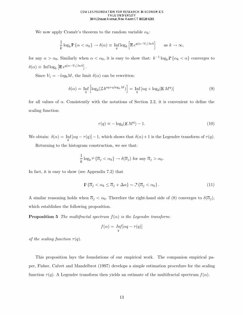
which establishes the following proposition.

Proposition 5 The multifractal spectrum f(α) is the Legendre transform:

f(α) = Infq

[αq − τ(q)]

of the scaling function τ(q).

This proposition lays the foundations of our empirical work. The companion empirical pa-

per, Fisher, Calvet and Mandelbrot (1997) develops a simple estimation procedure for the scaling

function τ(q). A Legendre transform then yields an estimate of the multifractal spectrum f(α).

13

The previous discussion showed that f(α) is the limit of:

k−1 logb P αk > α + 1 if α > α0,

k−1 logb P αk < α + 1 if α < α0,

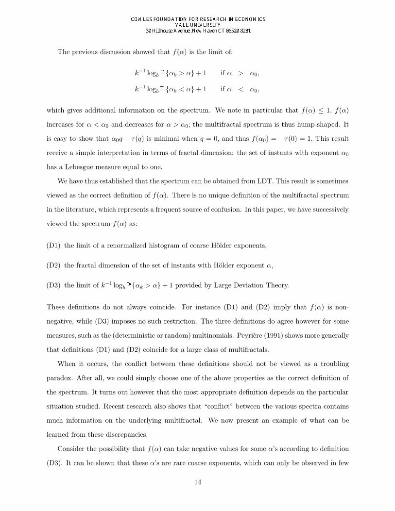
which gives additional information on the spectrum. We note in particular that f(α) ≤ 1, f(α)

increases for α < α0 and decreases for α > α0; the multifractal spectrum is thus hump-shaped. It

is easy to show that α0q − τ(q) is minimal when q = 0, and thus f(α0) = −τ(0) = 1. This result

receive a simple interpretation in terms of fractal dimension: the set of instants with exponent α0

has a Lebesgue measure equal to one.

We have thus established that the spectrum can be obtained from LDT. This result is sometimes

viewed as the correct definition of f(α). There is no unique definition of the multifractal spectrum

in the literature, which represents a frequent source of confusion. In this paper, we have successively

viewed the spectrum f(α) as:

(D1) the limit of a renormalized histogram of coarse Holder exponents,

(D2) the fractal dimension of the set of instants with Holder exponent α,

(D3) the limit of k−1 logb P αk > α + 1 provided by Large Deviation Theory.

These definitions do not always coincide. For instance (D1) and (D2) imply that f(α) is non-

negative, while (D3) imposes no such restriction. The three definitions do agree however for some

measures, such as the (deterministic or random) multinomials. Peyriere (1991) shows more generally

that definitions (D1) and (D2) coincide for a large class of multifractals.

When it occurs, the conflict between these definitions should not be viewed as a troubling

paradox. After all, we could simply choose one of the above properties as the correct definition of

the spectrum. It turns out however that the most appropriate definition depends on the particular

situation studied. Recent research also shows that “conflict” between the various spectra contains

much information on the underlying multifractal. We now present an example of what can be

learned from these discrepancies.

Consider the possibility that f(α) can take negative values for some α’s according to definition

(D3). It can be shown that these α’s are rare coarse exponents, which can only be observed in few

14

random measures. Such α’s, which are only revealed by examining a large number of measures,

are called latent. They contrast with manifest α’s for which f(α) > 0. Latent values have the

additional property to control the high and low moments of the measure. The spectrum given

by LDT thus contains information on the variability of sample histograms, which illustrates the

complementarity of these two definitions. Mandelbrot (1989b) provides further discussion of this

topic.

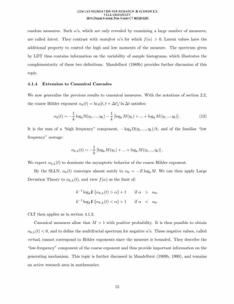
4.1.4 Extension to Canonical Cascades

We now generalize the previous results to canonical measures. With the notations of section 2.2,

the coarse Holder exponent αk(t) = lnµ[t, t+ ∆t]/ ln ∆t satisfies:

αk(t) = −1k

logb Ω(η1, ..., ηk) − 1k

[logbM(η1) + ...+ logbM(η1, .., ηk)] . (12)

It is the sum of a “high frequency” component, − logb Ω(η1, ..., ηk)/k, and of the familiar “low

frequency” average:

αk,L(t) = −1k

[logbM(η1) + ...+ logbM(η1, .., ηk)] .

We expect αk,L(t) to dominate the asymptotic behavior of the coarse Holder exponent.

By the SLLN, αk(t) converges almost surely to α0 = −E logbM. We can then apply Large

Deviation Theory to αk,L(t), and view f(α) as the limit of:

k−1 logb P αk,L(t) > α + 1 if α > α0,

k−1 logb P αk,L(t) < α + 1 if α < α0.

CLT then applies as in section 4.1.3.

Canonical measures allow that M > 1 with positive probability. It is then possible to obtain

αk,L(t) < 0, and to define the multifractal spectrum for negative α’s. These negative values, called

virtual, cannot correspond to Holder exponents since the measure is bounded. They describe the

“low-frequency” component of the coarse exponent and thus provide important information on the

generating mechanism. This topic is further discussed in Mandelbrot (1989b, 1990), and remains

an active research area in mathematics.

15

4.2 Examples

The new characterization of the multifractal spectrum given in (D3) is now used to derive explicit

formulae for f(α). These results are important for empirical work. They allow identification

of a multiplicative cascade from its multifractal spectrum. This method is implemented in the

companion empirical paper.

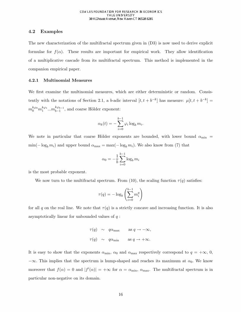
4.2.1 Multinomial Measures

We first examine the multinomial measures, which are either deterministic or random. Consis-

tently with the notations of Section 2.1, a b-adic interval [t, t + b−k] has measure: µ[t, t + b−k] =

mkϕ00 mkϕ1

1 ...mkϕb−1

b−1 , and coarse Holder exponent:

αk(t) = −b−1∑i=0

ϕi logbmi.

We note in particular that coarse Holder exponents are bounded, with lower bound αmin =

min(− logbmi) and upper bound αmax = max(− logbmi). We also know from (7) that

α0 = −1b

b−1∑i=0

logbmi

is the most probable exponent.

We now turn to the multifractal spectrum. From (10), the scaling function τ(q) satisfies:

τ(q) = − logb

(b−1∑i=0

mqi

)

for all q on the real line. We note that τ(q) is a strictly concave and increasing function. It is also

asymptotically linear for unbounded values of q :

τ(q) ∼ qαmax as q → −∞,

τ(q) ∼ qαmin as q → +∞.

It is easy to show that the exponents αmin, α0 and αmax respectively correspond to q = +∞, 0,

−∞. This implies that the spectrum is hump-shaped and reaches its maximum at α0. We know

moreover that f(α) = 0 and |f ′(α)| = +∞ for α = αmin, αmax. The multifractal spectrum is in

particular non-negative on its domain.

16

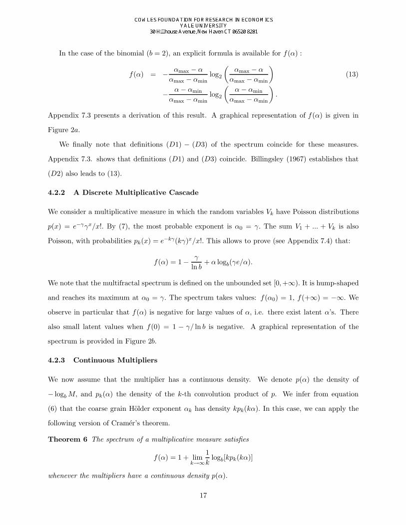
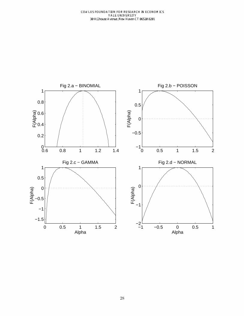
In the case of the binomial (b = 2), an explicit formula is available for f(α) :

f(α) = − αmax − α

αmax − αminlog2

(αmax − α

αmax − αmin

)(13)

− α− αmin

αmax − αminlog2

(α− αmin

αmax − αmin

).

Appendix 7.3 presents a derivation of this result. A graphical representation of f(α) is given in

Figure 2a.

We finally note that definitions (D1) − (D3) of the spectrum coincide for these measures.

Appendix 7.3. shows that definitions (D1) and (D3) coincide. Billingsley (1967) establishes that

(D2) also leads to (13).

4.2.2 A Discrete Multiplicative Cascade

We consider a multiplicative measure in which the random variables Vk have Poisson distributions

p(x) = e−γγx/x!. By (7), the most probable exponent is α0 = γ. The sum V1 + ... + Vk is also

Poisson, with probabilities pk(x) = e−kγ(kγ)x/x!. This allows to prove (see Appendix 7.4) that:

f(α) = 1 − γ

ln b+ α logb(γe/α).

We note that the multifractal spectrum is defined on the unbounded set [0,+∞). It is hump-shaped

and reaches its maximum at α0 = γ. The spectrum takes values: f(α0) = 1, f(+∞) = −∞. We

observe in particular that f(α) is negative for large values of α, i.e. there exist latent α’s. There

also small latent values when f(0) = 1 − γ/ ln b is negative. A graphical representation of the

spectrum is provided in Figure 2b.

4.2.3 Continuous Multipliers

We now assume that the multiplier has a continuous density. We denote p(α) the density of

− logbM, and pk(α) the density of the k-th convolution product of p. We infer from equation

(6) that the coarse grain Holder exponent αk has density kpk(kα). In this case, we can apply the

following version of Cramer’s theorem.

Theorem 6 The spectrum of a multiplicative measure satisfies

f(α) = 1 + limk→∞

1k

logb[kpk(kα)]

whenever the multipliers have a continuous density p(α).

17

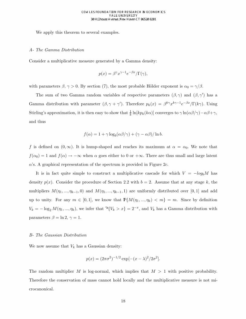
We apply this theorem to several examples.

A- The Gamma Distribution

Consider a multiplicative measure generated by a Gamma density:

p(x) = βγxγ−1e−βx/Γ(γ),

with parameters β, γ > 0. By section (7), the most probable Holder exponent is α0 = γ/β.

The sum of two Gamma random variables of respective parameters (β, γ) and (β, γ′) has a

Gamma distribution with parameter (β, γ + γ′). Therefore pk(x) = βkγxkγ−1e−βx/Γ(kγ). Using

Stirling’s approximation, it is then easy to show that 1k ln[kpk(kα)] converges to γ ln(αβ/γ)−αβ+γ,

and thus

f(α) = 1 + γ logb(αβ/γ) + (γ − αβ)/ ln b.

f is defined on (0,∞). It is hump-shaped and reaches its maximum at α = α0. We note that

f(α0) = 1 and f(α) → −∞ when α goes either to 0 or +∞. There are thus small and large latent

α’s. A graphical representation of the spectrum is provided in Figure 2c.

It is in fact quite simple to construct a multiplicative cascade for which V = −logbM has

density p(x). Consider the procedure of Section 2.2 with b = 2. Assume that at any stage k, the

multipliers M(η1, ..., ηk−1, 0) and M(η1, ..., ηk−1, 1) are uniformly distributed over [0, 1] and add

up to unity. For any m ∈ [0, 1], we know that PM(η1, ..., ηk) < m = m. Since by definition

Vk = − log2M(η1, ..., ηk), we infer that PVk > x = 2−x, and Vk has a Gamma distribution with

parameters β = ln 2, γ = 1.

B- The Gaussian Distribution

We now assume that Vk has a Gaussian density:

p(x) = (2πσ2)−1/2 exp[−(x− λ)2/2σ2].

The random multiplier M is log-normal, which implies that M > 1 with positive probability.

Therefore the conservation of mass cannot hold locally and the multiplicative measure is not mi-

crocanonical.

18

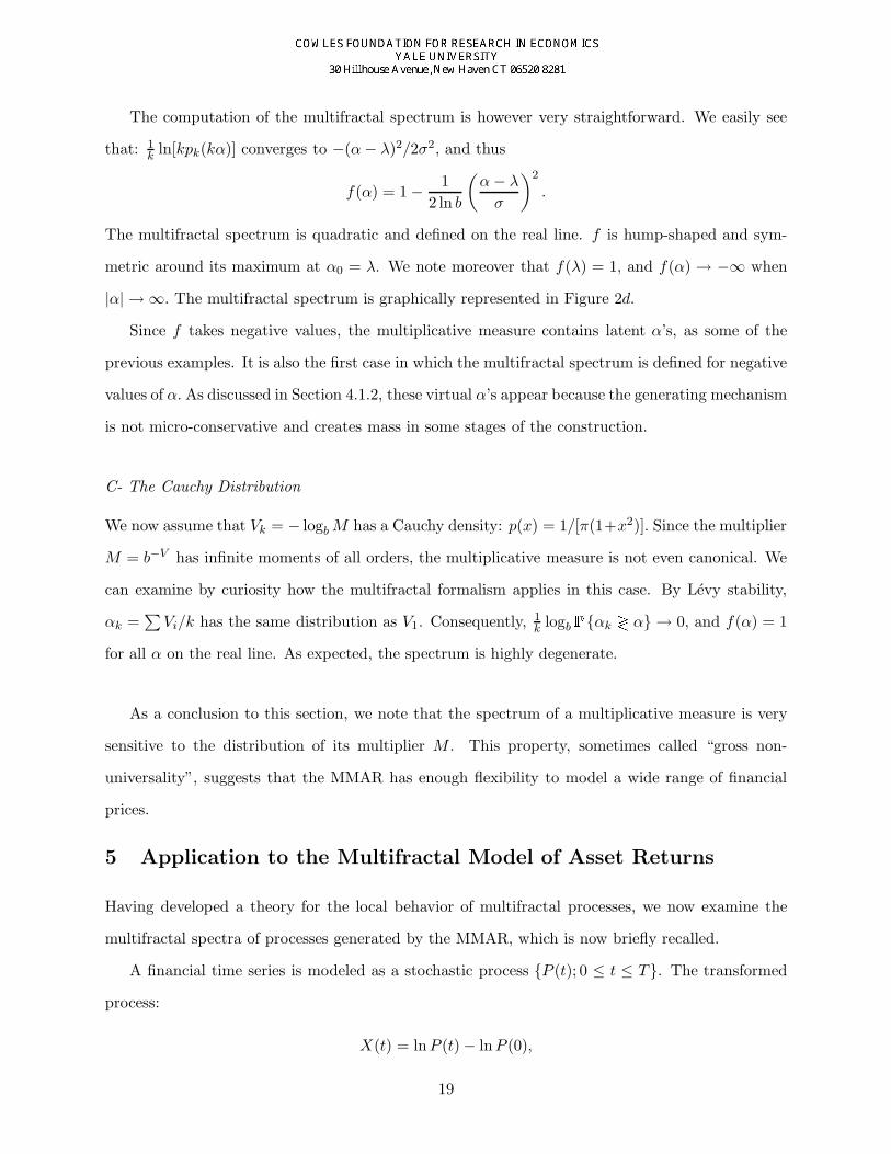
The computation of the multifractal spectrum is however very straightforward. We easily see

that: 1k ln[kpk(kα)] converges to −(α− λ)2/2σ2, and thus

f(α) = 1 − 12 ln b

(α− λ

σ

)2

.

The multifractal spectrum is quadratic and defined on the real line. f is hump-shaped and sym-

metric around its maximum at α0 = λ. We note moreover that f(λ) = 1, and f(α) → −∞ when

|α| → ∞. The multifractal spectrum is graphically represented in Figure 2d.

Since f takes negative values, the multiplicative measure contains latent α’s, as some of the

previous examples. It is also the first case in which the multifractal spectrum is defined for negative

values of α. As discussed in Section 4.1.2, these virtual α’s appear because the generating mechanism

is not micro-conservative and creates mass in some stages of the construction.

C- The Cauchy Distribution

We now assume that Vk = − logbM has a Cauchy density: p(x) = 1/[π(1+x2)]. Since the multiplier

M = b−V has infinite moments of all orders, the multiplicative measure is not even canonical. We

can examine by curiosity how the multifractal formalism applies in this case. By Levy stability,

αk =∑Vi/k has the same distribution as V1. Consequently, 1

k logb P αk ? α → 0, and f(α) = 1

for all α on the real line. As expected, the spectrum is highly degenerate.

As a conclusion to this section, we note that the spectrum of a multiplicative measure is very

sensitive to the distribution of its multiplier M . This property, sometimes called “gross non-

universality”, suggests that the MMAR has enough flexibility to model a wide range of financial

prices.

5 Application to the Multifractal Model of Asset Returns

Having developed a theory for the local behavior of multifractal processes, we now examine the

multifractal spectra of processes generated by the MMAR, which is now briefly recalled.

A financial time series is modeled as a stochastic process P (t); 0 ≤ t ≤ T. The transformed

process:

X(t) = lnP (t) − lnP (0),

19

is viewed as a multifractal compound process that satisfies the following properties.

Assumption 1. X(t) is a compound process:

X(t) ≡ BH [θ(t)]

where BH(t) is a fractional Brownian Motion with self-affinity index H, and θ(t) is a stochas-

tic trading time.

Assumption 2. The trading time θ(t) is the c.d.f. of a multifractal measure defined on [0, T ].

That is, θ(t) is a multifractal process with continuous, non-decreasing paths, and stationary

increments.

Assumption 3. BH(t) and θ(t) are independent.

While Mandelbrot, Fisher and Calvet (1997) studied the scaling properties of the MMAR in

terms of moments, this paper focuses on the local scaling properties of the price process. We denote

fθ(α) the multifractal spectrum of the process trading time and establish the following theorem.

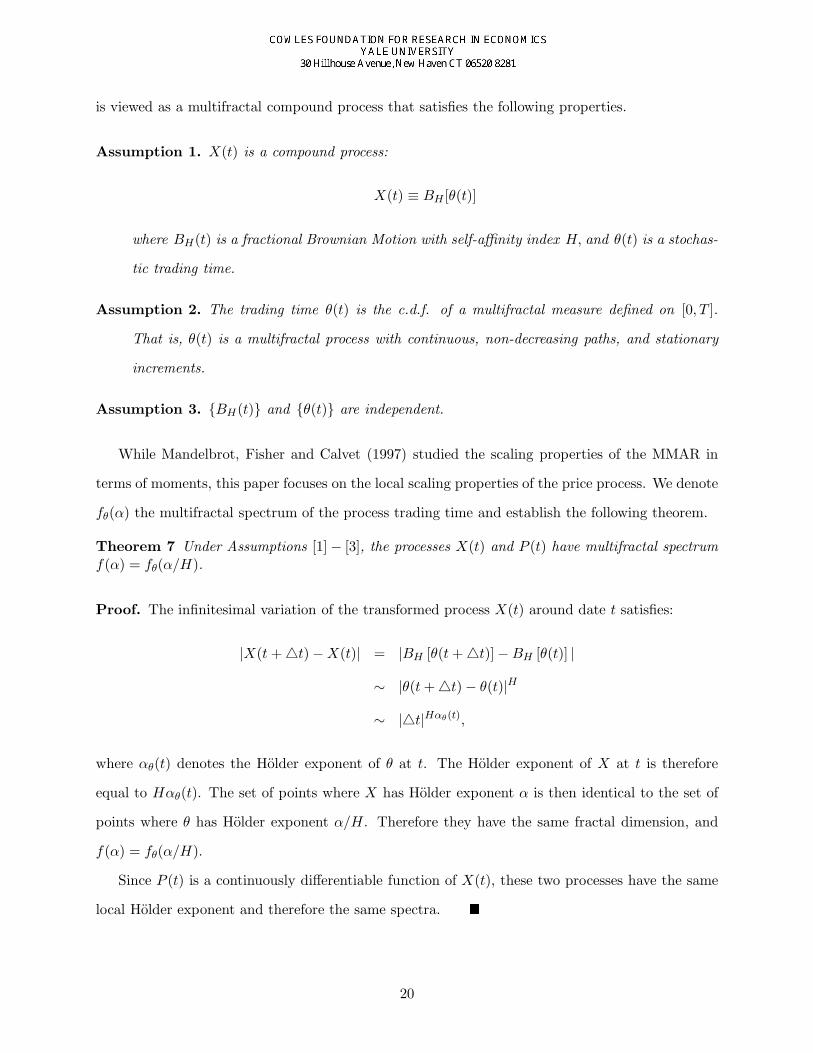
Theorem 7 Under Assumptions [1] − [3], the processes X(t) and P (t) have multifractal spectrumf(α) = fθ(α/H).

Proof. The infinitesimal variation of the transformed process X(t) around date t satisfies:

|X(t+ 4t) −X(t)| = |BH [θ(t+ 4t)] −BH [θ(t)] |

∼ |θ(t+ 4t) − θ(t)|H

∼ |4t|Hαθ(t),

where αθ(t) denotes the Holder exponent of θ at t. The Holder exponent of X at t is therefore

equal to Hαθ(t). The set of points where X has Holder exponent α is then identical to the set of

points where θ has Holder exponent α/H. Therefore they have the same fractal dimension, and

f(α) = fθ(α/H).

Since P (t) is a continuously differentiable function of X(t), these two processes have the same

local Holder exponent and therefore the same spectra.

20

Theorem 5.1 shows that the MMAR contains a continuum of local Holder exponents. Multi-

fractality of the compound price process is entirely caused by the trading time, and accounts for

scale consistency and persistence.

Long memory has an interesting geometric interpretation in this model. When the price process

is multiscaling, several sets6 T (α) have a non-integer fractal dimension f(α): 0 < f(α) < 1. Their

elements necessarily cluster in certain regions of the interval of definition [0, T ], which explains the

alternance of periods of large and small price changes. The set T (α) is also statistically self-similar

in the sense that after proper rescaling, subsets of T (α) have statistically the same spreading of

points than the original T (α). Therefore knowledge of T (α) in one period of time contains important

information on T (α) in later periods. This property accounts for long memory in the process.

6 Conclusion

This paper examines the local scaling properties of multifractals. Our analysis builds on the concept

of the local Holder exponent, a positive real number that quantifies a function’s singularity at a

given date. In the spirit of fractal geometry, these exponents are interpreted as local scaling factors

that can vary with time. Multifractals are then viewed as generalized fractal objects containing a

continuum of scales.

The distribution of local Holder exponents over time is described by the multifractal spectrum

f(α), a renormalized density obtained as the limit of histograms. In an alternative interpretation,

f(α) is viewed as the fractal dimension of the set of instants T (α) with local Holder exponent α.

The statistical self-similarity of the sets T (α) is closely related to the long memory. For a large class

of multifractals, the spectrum can be explicitly derived from Cramer’s Large Deviation Theory. We

apply this idea on a number of examples, and note the sensitivity of the multifractal spectrum to

the generating mechanism. This allows the applied researcher to relate an empirical estimate of

the spectrum back to a particular construction of the multifractal.

Finally, we apply these ideas to the Multifractal Model of Asset Returns (MMAR). The het-

erogeneity of local scales along the price process is entirely attributable to the trading time θ(t).

Moreover, the multifractal spectrum of the price process is derived from the spectrum of θ(t) by

a very simple transformation. The multiscaling properties of the MMAR sharply contrast with

6As in Section 3.3, we denote T (α) the set of instants with Holder exponent α.

21

the unique scale contained in previous financial models, including continuous Ito processes and

fractional Brownian motions. They account for the main features of the MMAR: scale-consistency,

fat tails, temporal heterogeneity and long memory in the magnitude of price changes. The results

of this paper also suggest several directions for empirical research, such as estimating the multi-

fractal spectrum and inferring the generating mechanism of a given price process. The companion

empirical paper, Fisher, Calvet and Mandelbrot (1997), proposes some solutions to these problems.

The development of estimation and inference methods for the MMAR should however be the focus

of further research.

22

7 Appendix

7.1 The Hausdorff-Besicovitch Dimension

We consider a bounded subset A of the Euclidean space Rn , (n ≥ 1). An open and countable

covering of A consists of a family of open subsets (Ui)∞i=1 that satisfies A ⊆ ∪∞i=1Ui. For any

positive real numbers s and ε, we define the quantity:

hsε(A) = Inf

∞∑i=1

diam(Ui)s | (Ui)∞i=1 open covering of A, diam(Ui) < ε for all i

.

As we decrease ε, the class of permissible coverings decreases, and the infimum increases. It thus

converges to a limit:

hs(A) = limε→0

hsε(A),

which belongs to [0,∞]. It is then possible to prove the following result.

Proposition 8 There exists a non-negative real number D(A) such that hs(A) = ∞ if s < D(A)and hs(A) = 0 if s > D(A). We call D(A) the fractal or Hausdorff-Besicovitch dimension of A.

The fractal dimension satisfies the following properties:

• If A ⊆ Rn , then D(A) ≤ n.

• If A ⊆ B, then D(A) ≤ D(B).

• If A is a countable set, then D(A) = 0.

7.2 Proof of Proposition 4.2

We easily see that:

P αj < αk ≤ αj + ∆α = P αk > αj − P αk > αj + ∆α

= Pαk > αj[1 − Pαk > αj + ∆α

Pαk > αj

]∼ Pαk > αj

The last equality follows from the fact that δ(αj + ∆α) < δ(αj), and thus that the ratio

Pαk > αj + ∆αPαk > αj

∼ (bk)δ(αj+∆α)−δ(αj)

vanishes as k → ∞.

23

7.3 Binomial Distribution

It is straightforward to compute f(α) by a Legendre transform of τ(q), which establishes (13) under

definition (D3).

The same result also holds under definition (D1). With the notations of Section 3.2, we consider

a fixed interval (αj , αj +∆α] and seek to compute the limit of log2Nk(αj)/k. The indices are chosen

so that αmax = − log2m0. After k iterations, the coarse Holder exponent of a b-adic interval is of

the form:

αk(t) = (αmax − αmin)ϕ0,k(t) + αmin,

where ϕ0,k(t) is the relative frequency of m0’s drawn in the construction. We observe that there is

a one-to-one correspondence between αk(t) and ϕ0,k(t). For this reason, it is convenient to define

ϕj =αj − αmin

αmax − αmin(14)

and ∆ϕ = ∆α/(αmax − αmin). The integer Nk(αj) can now be rewritten:

Nk(αj) = Cardti s.t. ϕ0,k(ti) ∈ (ϕj , ϕj + ∆ϕ]

=[k(ϕj+∆ϕ)]∑l=[kϕj ]+1

k

l

,

the last formula being obtained by a simple combinatorial argument.

We first consider the case αj > α0, i.e. ϕj > 1/2. The inequalities k

[kϕj ] + 1

≤ Nk(αj) ≤

([k(ϕj + ∆ϕ)] − [kϕj ]

) k

[kϕj] + 1

,

imply the useful equivalence

1k

log2Nk(αj) ∼1k

log2

k

[kϕj] + 1

as k → ∞.

Stirling ’s approximation can be applied to the right-hand side:

1k

log2Nk(αj) → −ϕj log2 ϕj − (1 − ϕj) log2(1 − ϕj).

Using (14), we substitute ϕj in this equation and obtain (13). A similar reasoning holds for αj < α0.

24

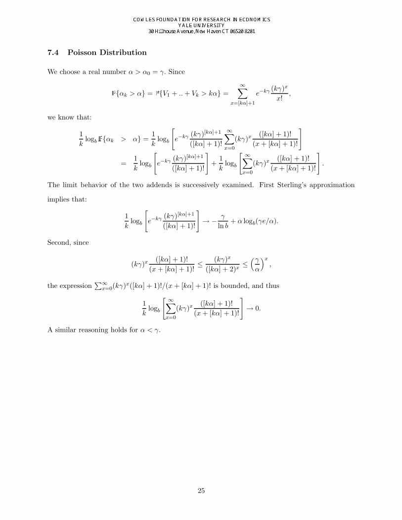
7.4 Poisson Distribution

We choose a real number α > α0 = γ. Since

Pαk > α = PV1 + ..+ Vk > kα =∞∑

x=[kα]+1

e−kγ (kγ)x

x!,

we know that:

1k

logb Pαk > α =1k

logb

[e−kγ (kγ)[kα]+1

([kα] + 1)!

∞∑x=0

(kγ)x ([kα] + 1)!(x+ [kα] + 1)!

]

=1k

logb

[e−kγ (kγ)[kα]+1

([kα] + 1)!

]+

1k

logb

[ ∞∑x=0

(kγ)x ([kα] + 1)!(x+ [kα] + 1)!

].

The limit behavior of the two addends is successively examined. First Sterling’s approximation

implies that:

1k

logb

[e−kγ (kγ)[kα]+1

([kα] + 1)!

]→ − γ

ln b+ α logb(γe/α).

Second, since

(kγ)x ([kα] + 1)!(x+ [kα] + 1)!

≤ (kγ)x

([kα] + 2)x≤(γα

)x,

the expression∑∞

x=0(kγ)x([kα] + 1)!/(x + [kα] + 1)! is bounded, and thus

1k

logb

[ ∞∑x=0

(kγ)x ([kα] + 1)!(x+ [kα] + 1)!

]→ 0.

A similar reasoning holds for α < γ.

25

References

[1] Billingsley (1967), Ergodic Theory and Information, New York: Wiley

[2] Deutschel, J. D., and Stroock, D. W. (1989), Large Deviations, New York: Academic Press

[3] Durrett, R. (1991), Probability: Theory and Examples, Pacific Grove, Calif.: Wadsworth &Brooks/Cole Advanced Books & Software

[4] Evertsz, C. J. G., and Mandelbrot, B. B. (1992), Multifractal Measures, in: Peitgen, H. O.,Jurgens, H., and Saupe, D. (1992), Chaos and Fractals: New Frontiers of Science, 921-953,New York: Springer Verlag

[5] Fisher, A., Calvet, L., and Mandelbrot, B. B. (1997), Multifractality of Deutschmark/USDollar Exchange Rates, Yale University, Working Paper

[6] Frisch, U., and Parisi, G. (1985), Fully Developed Turbulence and Intermittency, in: M. Ghiled., Turbulence and Predictability in Geophysical Fluid Dynamics and Climate Dynamics, 84-88, Amsterdam: North-Holland

[7] Halsey, T. C., Jensen, M. H., Kadanoff, L. P., Procaccia, I., and Shraiman, B. I. (1986), Frac-tal Measures and their Singularities: The Characterization of Strange Sets, Physical ReviewLetters A 33, 1141

[8] Hausdorff, F. (1919), Dimension und ausseres Mass, Mathematische Annalen 79 157-179

[9] Mandelbrot, B. B., and Ness, J. W. van (1968), Fractional Brownian Motion, Fractional Noisesand Application, SIAM Review 10, 422-437

[10] Mandelbrot, B. B. (1982), The Fractal Geometry of Nature, New York: Freeman

[11] Mandelbrot, B. B. (1989a), Multifractal Measures, Especially for the Geophysicist, Pure andApplied Geophysics 131, 5-42

[12] Mandelbrot, B. B. (1989b), Examples of Multinomial Multifractal Measures that Have Neg-ative Latent Values for the Dimension f(α), in: L. Pietronero ed., Fractals’Physical Originsand Properties, 3-29, New York: Plenum

[13] Mandelbrot, B. B. (1990), Limit Lognormal Multifractal Measures, in: E. A. Gotsman et al.eds., Frontiers of Physics: Landau Memorial Conference, 309-340, New York: Pergamon

[14] Mandelbrot, B. B., Fisher, A., and Calvet, L. (1997), The Multifractal Model of Asset Returns,Yale University, Working Paper

[15] Peyriere, J. (1991), Multifractal Measures, in Proceedings of the NATO ASI “ProbabilisticStochastic Methods in Analysis, with Applications”

[16] Rogers, C. A. (1970), Hausdorff Measures, Cambridge University Press

[17] Rossi, P. ed. (1997), Modeling Stock Market Volatility: Bridging the Gap to Continuous Time,New York: Academic Press

26

27

0.6 0.8 1 1.2 1.40

0.2

0.4

0.6

0.8

1Fig 2.a − BINOMIAL

F(A

lpha

)

0 0.5 1 1.5 2−1

−0.5

0

0.5

1Fig 2.b − POISSON

F(A

lpha

)

0 0.5 1 1.5 2

−1.5

−1

−0.5

0

0.5

1Fig 2.c − GAMMA

Alpha

F(A

lpha

)

−1 −0.5 0 0.5 1−2

−1

0

1Fig 2.d − NORMAL

Alpha

F(A

lpha

)

28