Embed Size (px)
Citation preview
LARGE EDDY SIMULATION OF FLOW OVER CYLINDRICAL BODIES USING
UNSTRUCTURED FINITE VOLUME MESHES
A thesis submitted to The University of Manchester for the degree of Doctor of Philosophy in the Faculty of Engineering and Physical Sciences
July 2007
Imran Afgan
School of Mechanical, Aerospace and Civil Engineering
2
Contents List of Figures 06 List of Tables 10 Abstract 11 Declaration 12 Copyright 13 Acknowledgements 14 Preface 16 Nomenclature 18 Chapter 1 . ...............................................................................23
INTRODUCTION TO TURBULENCE ............................................................ 23 1.1). TURBULENT SCALES OF MOTION......................................................... 23 1.2). VELOCITY PROFILES IN THE NEAR WALL REGION ......................... 25 1.3). TURBULENT FLOW HANDLING ............................................................. 26 1.4). EDDY VISCOSITY AND MIXING LENGTH THEORY........................... 27 1.5). TURBULENCE MODELLING .................................................................... 28 1.6). REYNOLDS ENSEMBLE AVERAGING ................................................... 29 1.7). REYNOLDS AVERAGED NAVIER-STOKES MODELS ......................... 30
1.7.1). k ε− MODEL ........................................................................................ 30 1.7.2). RNG k ε− MODEL............................................................................... 30 1.7.3). k ω− MODEL ....................................................................................... 31 1.7.4). MSST MODEL....................................................................................... 32 1.7.5). SSG REYNOLDS STRESS MODEL .................................................... 32
BIBLIOGRAPHY.................................................................................................. 37 Chapter 2 . ...............................................................................39
NON-STATISTICAL APPROACHES .............................................................. 39 2.1). DIRECT NUMERICAL SIMULATION ...................................................... 39 2.2). LARGE EDDY SIMULATION .................................................................... 40 2.3). FILTERING IN LES ...................................................................................... 40
2.3.1). FILTERED NAVIER STOKES EQUATIONS ..................................... 41 2.4). SUBGRID SCALE MODELLING ............................................................... 43
2.4.1). EDDY VISCOSITY MODELS.............................................................. 43 2.4.2). SMAGORINSKY MODEL.................................................................... 44 2.4.3). DYNAMIC SMAGORINSKY MODEL................................................ 46 2.4.4). WALL-ADAPTING LOCAL EDDY-VISCOSITY MODEL ............... 48
2.5). OTHER ASPECTS OF LES .......................................................................... 49 BIBLIOGRAPHY.................................................................................................. 51
Chapter 3 . ...............................................................................54
NUMERICAL TREATMENT ............................................................................ 54
3
3.1). CELL AND FACE BASE DEFINITIONS ................................................... 54 3.1.1). FACE SURFACE VECTORS................................................................ 54 3.1.2). CELL VOLUME .................................................................................... 54 3.1.3). CELL AND FACE VALUE CALCULATION...................................... 55 3.1.3). GRADIENT CALCULATION .............................................................. 55
3.2). TIME DISCRETIZATION............................................................................ 55 3.3). SPATIAL DISCRETIZATION ..................................................................... 56
3.3.1). FIRST ORDER UPWINDING............................................................... 56 3.3.2). SECOND ORDER UPWINDING.......................................................... 57 3.3.3). SECOND ORDER CENTRAL DIFFERENCING ................................ 57 3.3.4). BLEND OF FIRST ORDER AND SECOND ORDER SCHEMES...... 57
3.4). DIFFUSIVE FLUX TREATMENT .............................................................. 58 3.5). PRESSURE-VELOCITY COUPLING ......................................................... 58 BIBLIOGRAPHY.................................................................................................. 60
Chapter 4 . ...............................................................................61
CHANNEL FLOW .............................................................................................. 61 4.1). INTRODUCTION ......................................................................................... 61 4.2). LITERATURE REVIEW .............................................................................. 61 4.3). CASE DESCRIPTION .................................................................................. 63 4.4). GRID RESOLUTION ................................................................................... 64 4.5). NUMERICAL TREATMENT ...................................................................... 64 4.6). RESULTS AND DISCUSSIONS.................................................................. 66 4.7). CONCLUSIONS ........................................................................................... 68 BIBLEOGRAPHY................................................................................................. 75
Chapter 5 . ...............................................................................77
REVIEW OF FLOW AROUND FINITE CYLINDERS ................................. 77 5.1). INTRODUCTION ......................................................................................... 77 5.2). LITERATURE REVIEW FOR FINITE CYLINDERS ................................ 77
5.2.1). VORTEX SHEDDING BEHIND CYLINDERS ................................... 77 5.2.2). LIFT AND DRAG FORCES.................................................................. 79 5.2.3). PRESSURE FLUCTUATIONS AND CYLINDER VIBRATIONS ..... 80 5.2.4). NUMERICAL SIMULATION OF FLOWS AROUND CYLINDERS USING LES ........................................................................................................ 81
5.3). CONCLUDING REMARKS......................................................................... 83 BIBLIOGRAPHY.................................................................................................. 85
Chapter 6 . ...............................................................................89
LES OF FLOW AROUND FINITE CANTILEVER CYLINDERS ............... 89 6.1). INTRODUCTION ......................................................................................... 89 6.2). FLOW GEOMETRY..................................................................................... 90 6.3). NUMERICAL TREATMENT ...................................................................... 90 6.4). GRID DEPENDENCE STUDY .................................................................... 92 6.5). DISCUSSION OF RESULTS ....................................................................... 93
6.5.1). PRESSURE DISTRIBUTION................................................................ 93 6.5.2). VELOCITY DISTRIBUTION ............................................................... 95
4
6.5.3). LIFT, DRAG AND TURBULENCE INTENSITY................................ 98 6.6). CONCLUSIONS ........................................................................................... 99 BIBLIOGRAPHY................................................................................................ 117
Chapter 7 . .............................................................................120
REVIEW OF FLOW IN IN-LINE TUBE BUNDLES ................................... 120 7.1). INTRODUCTION ....................................................................................... 120 7.2). LITERATURE REVIEW OF FLOW IN TUBE BUNDLES...................... 120
7.2.1). LIFT AND DRAG COEFFICIENTS ................................................... 121 7.2.2). PRESSURE FLUCTUATIONS ........................................................... 122 7.2.3). STROUHAL NUMBER....................................................................... 123 7.2.4). VORTEX SHEDDING......................................................................... 123 7.2.5). VIBRATIONS IN TUBE BANKS....................................................... 125 7.2.6). VIBRATIONS IN CANTILEVERED TUBE BANKS ....................... 126
7.3). INVESTIGATION OF FLOW IN TUBE BANKS VIA NUMERICAL SIMULATIONS................................................................................................... 127 BIBLIOGRAPHY................................................................................................ 133
Chapter 8 . .............................................................................136
LES OF FLOW IN TUBE BUNDLES ............................................................. 136 8.1). INTRODUCTION ....................................................................................... 136 8.2). NUMERICAL TREATMENT .................................................................... 137 8.3). CASE DESCRIPTION ................................................................................ 138 8.4). GRID SENSITIVITY TESTS ..................................................................... 139 8.5). TWO-POINT CORRELATION TESTS ..................................................... 140 8.6). RESULTS AND DISCUSSIONS................................................................ 141
8.6.1). FLOW PHYSICS.................................................................................. 141 8.6.2). PRESSURE DISTRIBUTIONS AROUND CENTER CYLINDER ... 143 8.6.3). VELOCITY PROFILES AND TURBULENCE INTENSITIES......... 144 8.6.4). LIFT AND DRAG FORCES................................................................ 145
8.7). CONCLUSIONS ......................................................................................... 147 BIBLIOGRAPHY................................................................................................ 162
Chapter 9 . .............................................................................165
SIMULATION OF FLOW IN TUBE BUNDLES BY URANS ..................... 165 9.1). INTRODUCTION ....................................................................................... 165 9.2). CASE DESCRIPTION AND NUMERICS................................................. 166 9.3). RESULTS AND DISCUSSIONS................................................................ 167
9.3.1). FLOW PHYSICS.................................................................................. 167 9.3.2). VELOCITY PROFILES AND TURBULENCE INTENSITIES......... 169 9.3.3). LIFT AND DRAG FORCES................................................................ 170
9.4). CONCLUSIONS ......................................................................................... 170 BIBLIOGRAPHY................................................................................................ 181
Chapter 10 . ...........................................................................182
LES OF FLOW AROUND A GENERIC CAR MIRROR............................. 182 10.1). INTRODUCTION ..................................................................................... 182
5
10.2). LITERATURE REVIEW .......................................................................... 183 10.3). CASE DESCRIPTION AND NUMERICS............................................... 185 10.4). RESULTS AND DISCUSSIONS.............................................................. 186
10.4.1). FLOW PHYSICS................................................................................ 187 10.4.2). ACOUSTIC CALCULATIONS......................................................... 190
10.5). CONCLUSIONS ....................................................................................... 191 BIBLIOGRAPHY................................................................................................ 209
Conclusions 211 Appendix A – List of Publications 215 Appendix B – Non-Conforming Meshes 217 Appendix C – User Coding 232 Appendix D – LES Coding 264 Appendix E – Car Mirror Experimental Comparison 289
6
List of Figures Figure 1-1: Length scale ranges of eddies at very high Reynolds number36 Figure 1-2: Energy Spectrum vs. wave number space (log-log scale) ..... 36 Figure 3-1: A polyhedral cell with notation of quantities ........................... 59 Figure 3-2: Diffusive flux calculation across non-conforming grid cells .... 59 Figure 4-1: Channel flow geometry with dimensions of 2 2πδ δ πδ× × where
δ = 1....................................................................................... 70 Figure 4-2: Results of Case 1 (Smagorinsky model without damping) and
Case 2 (Smagorinsky model with Van-Driest wall damping), comparison is made with DNS data of Kim et al. (1987). (a): Mean velocity. (b): Mean streamwise stress. (c): Mean normal stress. (d): Mean spanwise stress. ........................................ 71
Figure 4-3: Results of Case 3 (WALE model) where WC = 0.28. (a): Mean velocity. (b): Mean streamwise stress. (c): Mean normal stress. (d): Mean spanwise stress..................................................... 72
Figure 4-4: Results of Case 4 (Dynamic Smagorinsky model). (a): Mean velocity. (b): Mean streamwise stress. (c): Mean normal stress. (d): Mean spanwise stress..................................................... 73
Figure 4-5: Comparison between Smagorinsky model, WALE model and dynamic Smagorinsky model. (a): Mean velocity. (b): Mean streamwise stress. (c): Mean normal stress. (d): Mean spanwise stress. .................................................................... 74
Figure 6-1: Geometry under consideration of finite cylinder. Top: Cross sectional view in XZ plane. Bottom: Cross sectional view in XY plane.....................................................................................102
Figure 6-2: Various orthogonal and sectional views of the grid for AR 10 case. (a): Non-conforming mesh with local refinement (FNCM1). (b): Regular mesh (CM). 3D view of the complete grid (top), sectional view in XZ plane (middle) and sectional view in XY plane (bottom).....................................................103
Figure 6-3: Cp profile around the cylinder. (a): Case1 (AR 10) at Z/L=0.883 (Experiment of Park and Lee (2000), CNCM1, FNCM1 and CM). (b): Case 2 (AR 6) at Z/L=0.5 (Experiment of Park and Lee (2002), CNCM2 and FNCM2) ........................................104
Figure 6-4: Pressure profile along cylinder axis, top: along stagnation line at 0 degrees, bottom: along wake line at 180 degrees. (a): AR 10 case. (b): AR 6 case ........................................................105
Figure 6-5: Cp profile along the cylinder surface. (a): AR 10 case (from top to bottom Z/L=0.983, Z/L=0.95, Z/L=0.933, Z/L=0.9 and Z/L=0.883 respectively). (b): AR 6 case (from top to bottom Z/L=0.983, Z/L=0.944, Z/L=0.917, Z/L=0.806 and Z/L=0.5 respectively) .........................................................................106
Figure 6-6: Streamlines generated from 2D mean velocity vectors in XY planes at various Z/L locations for AR 6 case (FNCM2). ......107
Figure 6-7: Streamlines generated from 2D mean velocity vectors in XZ (symmetry) plane for AR 6 case (FNCM2)............................108
Figure 6-8: Mean velocity comparison in the wake of the cylinders at various X/D locations. (a): AR 10 case. (b): AR 6 case ........109
7
Figure 6-9: Pseudo-average streamlines behind cylinder at various locations for AR 10 case (FNCM1) along with contours of secondary flow......................................................................110
Figure 6-10: XZ sectional views at Y/D=0 for AR 10 case (FNCM1). (a): Pseudo average streamlines. (b): Instantaneous Velocity magnitude.............................................................................111
Figure 6-11: Instantaneous velocity magnitude plots in XY plane. (a): AR 6 case (FNCM2). (b): AR 10 case (FNCM1)............................112
Figure 6-12: 2nd invariant of the velocity gradients ( 1)Q = rendered by contours of vorticity [ ]( / ) ( / )Z u y v xω = ∂ ∂ − ∂ ∂ . (a): AR 6 case (FNCM2). (b): AR 10 case (FNCM1). ...................................113
Figure 6-13: Lift and drag curves for AR 10 case (FNCM1). (b): PSD of lift coefficient for both cases (AR 10 FNCM1 and AR 6 FNCM2). (c): PSD of lift coefficient on a log-log scale for AR 10 case (FNCM1)...............................................................................114
Figure 6-14: Streamwise turbulence intensity (Tu%) at Z/L=0.5 and X/D=5 for AR 6 case. .......................................................................115
Figure 6-15: u u′ ′< > at various Z/L locations for AR 10 case. (a): Z/L=0.950. (b): Z/L=0.625. (c): Z/L=0.125...............................................116
Figure 7-1: Flow pattern in in-line tube bundles taken from Ishigai et al. (1973), where P is the horizontal distance between tube centers and T is the vertical distance....................................129
Figure 7-2: Strouhal number for square cylinder arrays against gap ratios taken from Weaver et al. (1986) ...........................................130
Figure 7-3: Picture taken from Sumner et al. (1999) showing biased deflection angle against T/D for two cylinders ......................131
Figure 7-4: Picture taken from Ogengoren and Zaida (1992), showing biased flow pattern for a resonant case................................132
Figure 8-1: Geometry of in-line tube bundle configuration ......................151 Figure 8-2: Cross-sectional view of the grid in XY (Z=3) and YZ (X=3)
plane. (a): Coarse mesh (CM) 0.69 million cells, (b): Fine mesh (FM) 1.3 million cells, (c) Very fine mesh (VFM) 2.4 million cells.............................................................................................152
Figure 8-3: Comparison of solution obtained with various grids, CM, FM and VFM for gap ratio 1.5. (a) CP along central cylinder, (b) streamwise velocity at X/D = 2.25.........................................153
Figure 8-4: Spanwise correlation of streamwise velocity obtained with LZ=2D, at different points in the flow domain for gap ratio 1.5. A: (1.5, 1.5), B: (3.0, 4.5), C: (4.5, 3.0), D: (4.75, 0.85).........154
Figure 8-5: Pseudo-average mean velocity streamlines for various gap ratios. (a): Gap ratio 1.2. (b): Gap ratio 1.5. (c): Gap ratio 1.5. (d): Gap ratio 1.6. (e): Gap ratio 1.75....................................155
Figure 8-6: Mean pressure contours in a XY cross sectional view at Z/D=1.0 for gap ratio 1.5 case corresponding to flow pattern of Figure 8-5(b).........................................................................156
Figure 8-7: Normalized Cp profile around centre cylinder. (a): 1.2 x 1.2, (b): 1.5 x 1.5, (c): 1.6 x 1.6, (d): 1.75 x 1.75 ................................157
Figure 8-8: Mean velocity contours in a XY cross sectional view at Z/D=1.0 for gap ratio 1.5 case............................................................158
8
Figure 8-9: Streamwise turbulence intensity and streamwise velocity profiles between center tube and wake cylinder. (a): Gap ratio 1.2 at X=3.6. (b): Gap ratio 1.5 at X=4.5. (c): Gap ratio 1.6 at X=4.8. (d): Gap ratio 1.75 at X=5.25.....................................159
Figure 8-10: Multiple slices for various quantities for gap ratio 1.5 case. (Slice 1): YZ plane, velocity contour lines at X=1.5. (Slice 2): YZ plane, velocity flood contours at X=4.5. (Slice 3): XY plane, mean velocity vector plot at Z/D=2. (Slice 4): XY plane, mean velocity flood contour at Z/D=2 .............................................160
Figure 8-11: Power Density Spectrum analysis of the lift force for various gap ratios. (a): Gap ratio 1.2. (b): Gap ratio 1.5. (c): Gap ratio 1.6. (d): Gap ratio 1.75..........................................................161
Figure 9-1: Front view of the grids used for URANS simulations in XY plane. (a): High Reynolds number mesh 0.697 million cells, (b): Low Reynolds number mesh 0.843 million cells ...................173
Figure 9-2: Mean Pressure distribution around centre cylinder (a) 2-D URANS comparison. (b) 3-D URANS comparison ...............174
Figure 9-3: Pseudo-average mean velocity streamlines for various 2-D models. (a): k ε− model (b): RNG k ε− (c): MSST (d): SSG (e): 3-D LES..........................................................................175
Figure 9-4: Pseudo-average mean velocity streamlines for various 3-D models. (a): k ε− model (b): RNG k ε− (c): MSST (d): SSG (e): LES ................................................................................176
Figure 9-5: Time averaged mean pressure distribution in XY plane at Z/D=1. (a): k ε− model (b): RNG k ε− (c): MSST (d): SSG (e) LES STAR-V4.......................................................................177
Figure 9-6: Pressure distribution around centre cylinder along with a sectional view in YZ plane at X=3.0. (a): k ε− model (b): RNG k ε− (c): MSST (d): SSG......................................................178
Figure 9-7: Comparisons between 3-D URANS and LES STAR-CD V4 behind central row of cylinders at X=4.5. (a): Mean velocity profile (b)Turbulence kinetic energy......................................179
Figure 9-8: Comparison of Reynolds stresses between 3-D SSG and LES STAR-V4 behind central cylinder at X=4.5. (a): u u′ ′< > (b):
v v′ ′< > (c): w w′ ′< > (d): u v′ ′< > ...........................................180 Figure 10-1: Computational domain for the generic car mirror..................195 Figure 10-2: Location of encapsulating blocks and their grids for various
meshes. (a): Coarse Mesh (CM) containing CF1. (b): Medium Mesh (MM) containing MF1. (c): Fine Mesh (FM) containing FF1 and FF2.........................................................................196
Figure 10-3: Zoomed in view for the Fine Mesh (FM) (a): XZ cross section (b): Mirror geometry (c): Behind mirror (d): XY cross section197
Figure 10-4: Separation line location for car mirror (a): Oil flow visualizations (b): Wall shear stress computed by Fine Mesh (FM) (c) LES Ask and Davidson (2006) (d) DES Ask and Davidson (2006).............................................................................................198
Figure 10-5: Normalized mean velocity profiles in mirror wake in centre plane (Y=0) (a) Graphical interpretation of the location of
9
reattachment point (b) Numerical LES (MM) and (FM) predictions ............................................................................199
Figure 10-6: Cross sectional views of various quantities in XZ plane at Y=0 for LES (FM). (a): Mean pressure (b): Mean velocity (c):
20/′ ′< >u u U (d): 2
0/′ ′< >v v U ..................................................200 Figure 10-7: Mean velocity contours at different Z/D heights in XY plane.
(a): Z/D=0.25 (b) Z/D=0.5 (c): Z/D=1 (d): Z/D=1.5 ................201 Figure 10-8: Classical horse shoe vortex interpretation (a): Iso-Q structures
(b) Normalized mean velocity showing location of horseshoe vortex....................................................................................202
Figure 10-9: Graphical interpretation of the location of horseshoe vortex.203 Figure 10-10: Cp profile along surface of the cylinder (a): Surface pressure
sensor locations on windward side (b): Surface pressure sensor locations on leeward side (c): Exp measurements and LES (FM) surface pressures.................................................204
Figure 10-11: Instantaneous drag (top curve), side (mid curve) and lift (bottom curve) coefficients for the LES (FM) simulation plotted against non-dimensionalised time tU/D ................................205
Figure 10-12: (a): Sensor location 116 (b): Pressure fluctuation levels for LES (FM) at Re=3.2 x 10⁵ and measured pressure fluctuation levels at Re=5.2 x 10⁵.....................................................................206
Figure 10-13: (a): Sensor location 119 (b): Pressure fluctuation levels for LES (FM) at Re=3.2 x 10⁵ and measured pressure fluctuation levels at Re=5.2 x 10⁵.....................................................................207
Figure 10-14: (a): Sensor location 123 (b): Pressure fluctuation levels for LES (FM) at Re=3.2 x 10⁵ and measured pressure fluctuation levels at Re=5.2 x 10⁵.....................................................................208
10
List of Tables Table 1-1: Some of the relevant quantities of turbulence modelling .......... 34 Table 1-2: Model coefficients for k ε− model............................................ 34 Table 1-3: Model coefficients for RNG k ε− model................................... 34 Table 1-4: Model coefficients for k ω− model ........................................... 34 Table 1-5: Model coefficients for MSST model .......................................... 34 Table 1-6: Model constants for ε equation for RSM model....................... 35 Table 6-1: Overview of the grid dependence study: Cases simulated,
meshes tested for each case and the total number of cells in each mesh...............................................................................101
Table 6-2: Strouhal number comparison ..................................................101 Table 8-1: Flow behaviour for tube bundles with various gap ratios. ∗ :AR <
1.2, ×:AR 1.2, :AR 1.5, ⊗ :AR 1.6, ⊕ :AR 1.75..............149 Table 8-2: Lift, drag and their root mean square values for all gap ratios.150 Table 8-3: Strouhal number comparison based on free stream velocity...150 Table 9-1: Size of the computational grids used.......................................172 Table 9-2: Lift, drag and their root mean square values for all gap ratios.172 Table 10-1: Size of the computational grids in millions...............................192 Table 10-2: Breakdown of encapsulating blocks showing their total number of
cells in millions and the block dimensions ...............................192 Table 10-3: Surface pressure sensor locations ..........................................193 Table 10-4: Pressure fluctuation level monitoring sensor locations............194
11
Abstract The thesis deals with the development and application of Large Eddy Simulation (LES) using unstructured meshes for industrial applications. Various sub-grid scale closure techniques namely, the classical Smagorinsky, Wall Adapting Local Eddy Viscosity and Dynamic Smagorinsky models have been implemented in a prototype version of the commercial code STAR-CD V4. For the development part, flow in a simple channel geometry was simulated with different types of meshes; regular, hexahedral, tetrahedral and polyhedral. The effects of mesh resolution, non-conforming grids, numerical discretizations and SGS modelling were studied in depth and a platform was established for application to industrial grade projects. The first test case consisted of finite cantilever cylinders of various aspect ratios mounted vertically on a flat plate. The cases were simulated using LES incorporating non-conforming meshes taking into consideration both the end tip and base effects of the cylinder. The second test case was that of tube bundles. These are widely used in nuclear and coal power plant heat exchangers and are thus of high importance. The high asymmetry of the flow and the effect of different gap ratios between tubes were also studied. The results were then compared to 2-D and 3-D Unsteady Reynolds-Averaged Navier-Stokes (URANS) models. The final case was the numerical simulation of flow around a generic side mirror of a car. This last case was simulated with polyhedral-cell meshes and prismatic-cell layers near solid walls; mirror surface and flat plate. The aerodynamic flow analysis was performed in conjunction with aeroacoustic study. The results from these industrial test cases were found to be very promising and encouraging for future applications of LES. As a whole the thesis looks into details of both the numerical aspects and the application difficulties of various LES models. Later, these models are applied to understand and discuss the flow physics of aforementioned industrial problems.

12
Declaration No portion of the work referred to in this thesis has been submitted in support of an application for another degree or qualification to this or any other university and/or institute of learning.
13
Copyright Copyright in the text of this thesis rests with the author. Copies (by any process) either in full, or of extracts, may be made only in accordance with instructions given by the author and lodged in John Rylands University Library of Manchester. Details may be obtained from the Librarian. This page must form part of any such copies made. Further copies (by any process) of copies made in accordance with such instructions may not be made without the permission (in writing) of the author. The ownership of any intellectual property rights which may be described in this thesis is vested in The University of Manchester, subject to any prior agreement to the contrary, and may not be made available for use by third parties without the written permission of the University, which will prescribe the terms and conditions of any such agreement. Further information on the conditions under which disclosures and exploitation may take place is available from the Head of School of Mechanical, Aerospace and Civil Engineering.

14
Acknowledgement I would like to thank Professor Dominique Laurence for his continued effort and support during the entire course of my PhD without which I would not have been able to come so far. I would also like to thank to Dr. Robert Prosser and other faculty members whose technical advice and knowledge helped me a lot. The funding and support given to me by the government of Pakistan (Higher Education Commission) and the European Union DESider project is much appreciated. I am also highly grateful to CD-adapco for their technical support and for providing me with the prototype version of STAR-CD V4 to work with. Special thanks to my office mates, Melih Guleren, Rizwan Riaz, Shafique-ur-Rehman and all others including Patricia Shepard for their continued support and encouragement. My sincere thanks to my friends back home especially, Ali, Omair, Kafeel, Assad, Farhan, Yasser, Billal and all others for being there whenever I needed moral support or technical help. I also wish to thank Ahad Khan who has been a dear friend for the last 4 years. I will surely miss his company and his sense of humor. I would also like to thank my parents, my brother and my sisters who have helped me in achieving all my goals. My deepest thanks to my wife Sumera for whose continued support has made me achieve both my distant and immediate goals. In the end I would like to offer special thanks to Dr. Charles Moulinec for who has been both a friend and a mentor to me over the last four years. His persistent support and technical feed back has enabled me to achieve a lot.

15
This work is dedicated to my wife Sumera and to my parents Tanvir and Naila
16
Preface The advancement in technology has made the implementation of numerical methods for the solution of fluid mechanics problems possible, leading to the progression of the field of Computational Fluid Dynamics (CFD). The solution of linear and non-linear systems of non-exact equations which was not a possibility in the past has become a reality via the rigorous iterative or exact techniques implemented through modern age computing. Even the most complex of fluid mechanics problems can be handled by Finite Difference, Finite Volume, or by Finite Element techniques. The former two techniques were specifically aimed at the solution of fluid mechanics problems and the latter was originally developed to handle structural problems. However, this technique has over the years also been advanced to handle fluid flow problems. In the current context only Finite Volume techniques will be discussed and implemented. Within the context of fluid mechanics the problems can be broadly categorized into steady and unsteady laminar, transitional and turbulent flows. Though the governing equations for all fluid flow problems are essentially the same, fluid flow behaviour however is quite different for these regimes. For laminar flows a simple iterative solution of the discretized Navier-Stokes equations leads to the final solution. However, for turbulent flows the scales of motion become considerably smaller. The scales of motion are directly related to the Reynolds number. As the Reynolds number increases the length scales decrease in size, requiring finer grids, thus making the simulations more and more costly in terms of computational power. Such a technique in which all the scales of motion are resolved for a turbulent flow is called Direct Numerical Simulation (DNS). At high Reynolds number the possibility of resolving all the scales of motion thus becomes unrealistic with the current computational power. Admittedly, some DNS have been performed for moderate Reynolds numbers for simple cases i.e. Kim et al. (1986)1 and Iwamoto et al. (2005)2. However, the current computational requirement for the application of DNS for high Reynolds flows is far from reality. Under such circumstances Reynolds Averaged Navier-Stokes (RANS) modelling is utilized. The RANS approach is based on the ensemble averaging of The Navier-Stokes equations, which are then solved via various types of turbulence models. Most of the RANS models, especially the one and two equation models, are based on the assumption that the turbulence is isotropic and that stresses can be directly related to strains. This is known as the Boussinesq hypothesis. In many cases, models based on this Boussinesq hypothesis approach perform very well. However, for cases which include highly swirling flows and stress-driven secondary flows such an 1Kim, J., Moin, P., Moser, R. 1986. Turbulence statistics in fully developed channel flow at low Reynolds number. J. of Fluid Mech. Vol 177, 133-166 2 Iwamoto, k., Kasagi, N., Suzuki, Y. 2005. Direct Numerical Simulation of channel flow at Re=2,320. Proc. 6th Symp. Smart Control of Turbulence, Tokyo
17
approach does not hold since turbulence is no longer isotropic. To model such anisotropic flows Reynolds stress models (RSM) are utilized which solve transport equations for all the Reynolds stresses. The computational burden of the solution of seven additional equations is sometimes immense, and is also accompanied with convergence problems. This makes the applicability of RSM models questionable. An intermediate approach still exists between DNS and RANS where only the large scales of motion (which are flow dependent) are resolved much like DNS. However, the smaller scales, which are universal in nature and are flow and Reynolds number independent, are modelled. This approach is called Large Eddy Simulation (LES). Such an approach puts LES on the intermediate boundary of DNS and RANS in terms of both computational power and solution accuracy. Most of the work in the context of this thesis is done using various models of LES. In some instances URANS approach is also implemented to study the differences in results between LES and URANS. Admittedly, LES is also quite expensive in terms of computational power, especially for higher Reynolds number flows where the scales of motion vary considerably. In a quest for the reduction of computing power special treatments such as wall functions and non-conforming meshes are to be implemented. For the current thesis such approaches are implemented and discussed in detail in the corresponding chapters of industrial applications of LES. Another aim of the present study is to test and compare the capabilities of URANS models with LES for flows around cylinders. Basics about turbulence and its modelling, the Finite Volume approach, DNS and LES will be discussed in the earlier chapters of this thesis, mainly Chapters 1 to 3. The benchmarking of various LES models for channel flow is shown in Chapter 4. The effects of grid resolution in particular the non-conforming meshes, and solution accuracies for channel flow are reported in Appendix B. Some quick fixes are also discussed for non-conforming meshes which are later utilized in the practical cases. In subsequent chapters various test cases are studied involving both experimental and numerical simulations. The different aspects of flow around cylinders are taken into consideration which include vortex shedding, cylinder aspect ratios, 3-D fluctuations in the wake, lift and drag (instantaneous and root mean squared) and pressure distributions. Chapters 5 and 6 will discuss flow over cantilever cylinders of various aspect ratios whereas in Chapters 7, 8 and 9 we shall discuss the flow over square in-line tube bundle arrays with various gap ratios. In tube banks the strong fluid structure coupling forces act as a cyclic load on tubes insides heat exchangers and nuclear power plants, and in time cause extensive wear and tear and in some cases even breakdowns. Finally in the last chapter of this thesis, the flow over the side mirror of a car will be discussed, which is simulated using an entirely different approach of polyhedral control volumes.
18
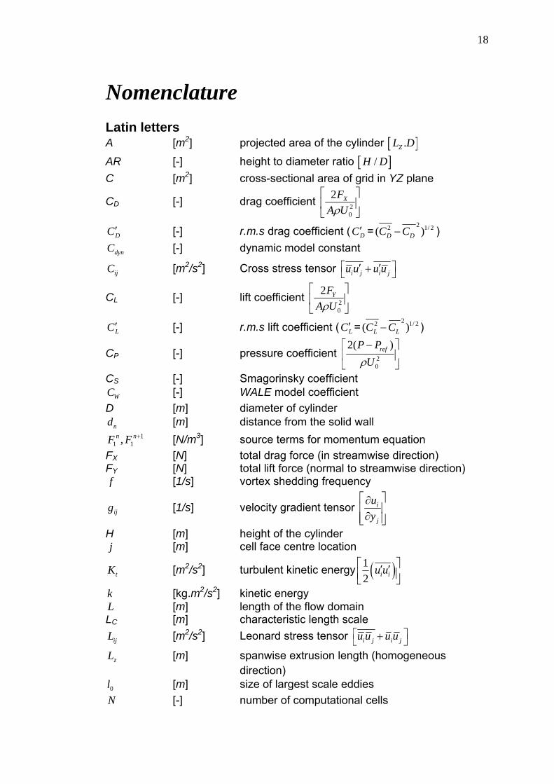
Nomenclature Latin letters A [m2] projected area of the cylinder [ ].ZL D
AR [-] height to diameter ratio [ ]/H D C [m2] cross-sectional area of grid in YZ plane
CD [-] drag coefficient 20
2 XFA Uρ
⎡ ⎤⎢ ⎥⎣ ⎦
DC ′ [-] r.m.s drag coefficient ( DC ′ =22 1/ 2( )D DC C− )
dynC [-] dynamic model constant
ijC [m2/s2] Cross stress tensor i j i ju u u u⎡ ⎤′ ′+⎣ ⎦
CL [-] lift coefficient 20
2 YFA Uρ
⎡ ⎤⎢ ⎥⎣ ⎦
LC ′ [-] r.m.s lift coefficient ( LC ′ =22 1/ 2( )L LC C− )
CP [-] pressure coefficient 20
2( )refP PUρ−⎡ ⎤
⎢ ⎥⎣ ⎦
CS [-] Smagorinsky coefficient WC [-] WALE model coefficient
D [m] diameter of cylinder nd [m] distance from the solid wall
11 1,n nF F + [N/m3] source terms for momentum equation
FX [N] total drag force (in streamwise direction) FY [N] total lift force (normal to streamwise direction) f [1/s] vortex shedding frequency
ijg [1/s] velocity gradient tensor i
j
uy
⎡ ⎤∂⎢ ⎥∂⎢ ⎥⎣ ⎦
H [m] height of the cylinder j [m] cell face centre location
tK [m2/s2] turbulent kinetic energy ( )12 i iu u⎡ ⎤′ ′⎢ ⎥⎣ ⎦
k [kg.m2/s2] kinetic energy L [m] length of the flow domain LC [m] characteristic length scale
ijL [m2/s2] Leonard stress tensor i j i ju u u u⎡ ⎤+⎣ ⎦
zL [m] spanwise extrusion length (homogeneous direction)
0l [m] size of largest scale eddies N [-] number of computational cells
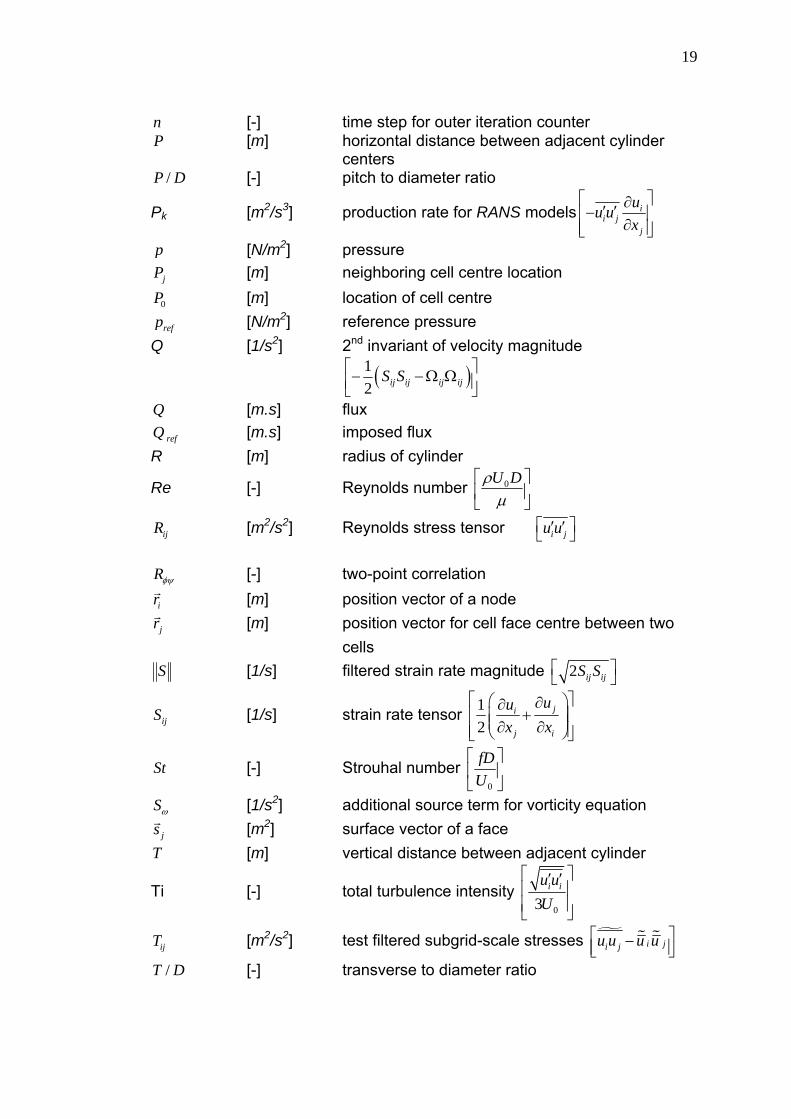
19
n [-] time step for outer iteration counter P [m] horizontal distance between adjacent cylinder
centers /P D [-] pitch to diameter ratio
Pk [m2/s3] production rate for RANS models ii j
j
uu ux
⎡ ⎤∂′ ′−⎢ ⎥∂⎢ ⎥⎣ ⎦
p [N/m2] pressure
jP [m] neighboring cell centre location
0P [m] location of cell centre
refp [N/m2] reference pressure Q [1/s2] 2nd invariant of velocity magnitude
( )12 ij ij ij ijS S⎡ ⎤− − Ω Ω⎢ ⎥⎣ ⎦
Q [m.s] flux
refQ [m.s] imposed flux R [m] radius of cylinder
Re [-] Reynolds number 0U Dρµ
⎡ ⎤⎢ ⎥⎣ ⎦
ijR [m2/s2] Reynolds stress tensor i ju u⎡ ⎤′ ′⎣ ⎦
Rφψ [-] two-point correlation
ir [m] position vector of a node
jr [m] position vector for cell face centre between two cells
S [1/s] filtered strain rate magnitude 2 ij ijS S⎡ ⎤⎣ ⎦
ijS [1/s] strain rate tensor 12
ji
j i
uux x
⎡ ⎤⎛ ⎞∂∂+⎢ ⎥⎜ ⎟⎜ ⎟∂ ∂⎢ ⎥⎝ ⎠⎣ ⎦
St [-] Strouhal number 0
fDU
⎡ ⎤⎢ ⎥⎣ ⎦
Sω [1/s2] additional source term for vorticity equation
js [m2] surface vector of a face T [m] vertical distance between adjacent cylinder
Ti [-] total turbulence intensity 03
i iu uU
⎡ ⎤′ ′⎢ ⎥⎢ ⎥⎣ ⎦
ijT [m2/s2] test filtered subgrid-scale stresses i ji ju u u u⎡ ⎤−⎢ ⎥⎣ ⎦
/T D [-] transverse to diameter ratio
20
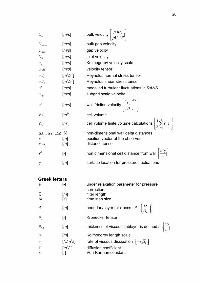
bU [m/s] bulk velocity Re2
b
bUµ
ρ δ⎡ ⎤⎢ ⎥⎣ ⎦
BGapU [m/s] bulk gap velocity
gapU [m/s] gap velocity
0U [m/s] inlet velocity uη [m/s] Kolmogorov velocity scale
,i ju u [m/s] velocity tensor
i iu u′ ′ [m2/s2] Reynolds normal stress tensor
i ju u′ ′ [m2/s2] Reynolds shear stress tensor
iu′′ [m/s] modelled turbulent fluctuations in RANS
sgsu [m/s] subgrid scale velocity
*u [m/s] wall friction velocity 1/ 2
wτρ
⎡ ⎤⎛ ⎞⎢ ⎥⎜ ⎟⎢ ⎥⎝ ⎠⎣ ⎦
olV [m3] cell volume
0PV [m3] cell volume finite volume calculations 1
1 .3
n
j jj
r s=
⎡ ⎤⎢ ⎥⎣ ⎦
∑
, ,X Y Z+ + +∆ ∆ ∆ [-] non-dimensional wall delta distances x [m] position vector of the observer
,i jx x [m] distance tensor
Y+ [-] non dimensional cell distance from wall *u yv
⎡ ⎤⎢ ⎥⎣ ⎦
y [m] surface location for pressure fluctuations Greek letters β [-] under relaxation parameter for pressure
correction ∆ [m] filter length
t∆ [s] time step size
δ [m] boundary layer thickness 0
vxU
δ⎡ ⎤⎛ ⎞⎢ ⎥⎜ ⎟⎢ ⎥⎝ ⎠⎣ ⎦∼
ijδ [-] Kronecker tensor
Subδ [m] thickness of viscous sublayer is defined as *
5vu
⎡ ⎤⎢ ⎥⎣ ⎦
η [m] Kolmogorov length scale
vε [N/m2s] rate of viscous dissipation ij ijSτ⎡ ⎤−⎣ ⎦ Γ [m2/s] diffusion coefficient κ [-] Von-Karman constant
21
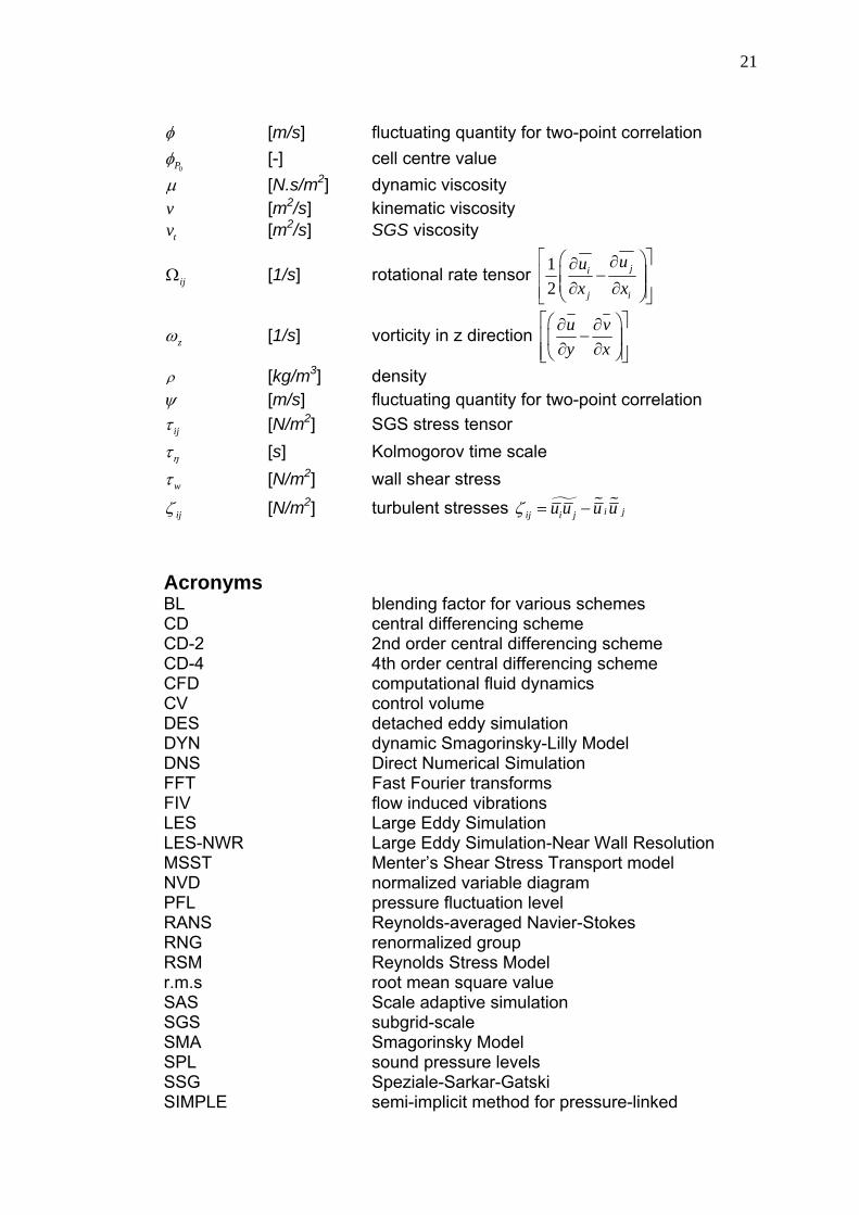
φ [m/s] fluctuating quantity for two-point correlation
0Pφ [-] cell centre value µ [N.s/m2] dynamic viscosity v [m2/s] kinematic viscosity
tv [m2/s] SGS viscosity
ijΩ [1/s] rotational rate tensor 12
ji
j i
uux x
⎡ ⎤⎛ ⎞∂∂⎢ − ⎥⎜ ⎟⎜ ⎟∂ ∂⎢ ⎥⎝ ⎠⎣ ⎦
zω [1/s] vorticity in z direction u vy x
⎡ ⎤⎛ ⎞∂ ∂−⎢ ⎥⎜ ⎟∂ ∂⎢ ⎥⎝ ⎠⎣ ⎦
ρ [kg/m3] density ψ [m/s] fluctuating quantity for two-point correlation
ijτ [N/m2] SGS stress tensor
ητ [s] Kolmogorov time scale
wτ [N/m2] wall shear stress
ijζ [N/m2] turbulent stresses i jij i ju u u uζ = −
Acronyms BL blending factor for various schemes CD central differencing scheme CD-2 2nd order central differencing scheme CD-4 4th order central differencing scheme CFD computational fluid dynamics CV control volume DES detached eddy simulation DYN dynamic Smagorinsky-Lilly Model DNS Direct Numerical Simulation FFT Fast Fourier transforms FIV flow induced vibrations LES Large Eddy Simulation LES-NWR Large Eddy Simulation-Near Wall Resolution MSST Menter’s Shear Stress Transport model NVD normalized variable diagram PFL pressure fluctuation level RANS Reynolds-averaged Navier-Stokes RNG renormalized group RSM Reynolds Stress Model r.m.s root mean square value SAS Scale adaptive simulation SGS subgrid-scale SMA Smagorinsky Model SPL sound pressure levels SSG Speziale-Sarkar-Gatski SIMPLE semi-implicit method for pressure-linked
22
equations TRANS transient Reynolds-averaged Navier-Stokes UD upwind scheme URANS unsteady Reynolds-averaged Navier-Stokes WALE Wall-Adapting Local Eddy Viscosity Other Symbols ( )′ fluctuating component
( ) filtered quantity
( ) mean
( ) test filter ^ Fourier space + non-dimensional wall value → vector sgs subgrid-scale
⟨ ⟩ time averaged quantity
CHAPTER 1. INTRODUCTION TO TURBULENCE 23
Chapter 1 .
INTRODUCTION TO TURBULENCE Turbulence is a 3-D phenomenon having complex and irregular dissipative behaviour. In turbulent flows the fluid velocity and pressure vary significantly and irregularly both in time and in space. We may even say that the flow itself is chaotic and random in nature. Due to this irregular motion a lot of desirable and undesirable effects are attained. For example in highly turbulent flows mixing of species takes place very rapidly as compared to laminar flow. This mixing of species is often desirable in chemical processes or inside engines for the mixing of air and fuel. On the other hand turbulence greatly increases the mixing of momentum of the fluid thus leading to undesirable effects such as high drag forces when it comes to aerospace applications.
1.1). TURBULENT SCALES OF MOTION Turbulent motions may vary in size from very large scales (comparable to flow geometry diameter) to very small scales (Kolmogorov scales-size of the smallest eddy) which become even smaller with an increase in flow Reynolds number. This means that a turbulent flow has eddies of different sizes ranging from very large to very small. The largest scale eddies have a characteristic length scale 0l , with the largest of them having a length scale comparable to the geometric length scale l . These large eddies are unstable and with time break up into smaller eddies transferring their energy. This transfer of energy is characterized by the dissipation ε . These smaller eddies undergo a similar process and break up into yet smaller eddies, this process continues until very small scale eddies are generated (their length scale is very much smaller than flow scale, 0l l ) which are stable but whose energy is so small that the viscous forces become dominant enough to overcome them. Thus in time these smallest eddies vanish dissipating their kinetic energy due to viscous effects. This process is known as the energy cascade and was first proposed by Richardson (1922). Suppose that the largest eddies have a velocity of 0u then their energy will be proportional to 2
0u ; a time scale will be 0 0 0/l uτ = and rate of transfer of energy will be 2 30 0
0 0
u ulτ
= . This basic concept originally given by Richardson was later refined
CHAPTER 1. INTRODUCTION TO TURBULENCE 24
by Kolmogorov (1941) who not only explained the energy cascade process but also defined the smallest scales of motion. Kolmogorov (1941) proposed three hypotheses, the first one of them was about the local isotropy, the statistics of small scale motions have a universal form which is uniquely determined by v and ε , unlike the large eddies which are anisotropic and directional in nature. If an imaginary demarcation is made of length scale EIl such that 0 / 6EIl l≈ then we may say that the isotropic small scales are eddies which are sufficiently smaller than EIl , ( EIl l< ). Kolmogorov further argued that the small eddies are not only isotropic but are also universal in nature. He proposed that as the large eddies break down transferring their energy they not only lose their directional information but also any other information regarding their geometry, thus making the smaller eddies some what universal in nature. These smaller eddies which are now universal in nature depend upon two primary parameters, the rate of transfer of energy EIT and the kinematic viscosity v . EIT is almost equal to the rate of dissipation ( EITε ≈ ). This was Kolmogorov's second hypothesis. Based on these two important parameters (ε and v ) Kolmogorov proposed length (η ), velocity (uη ) and time scales ( ητ ) for these universal eddies by dimensional analysis as
1/ 43vηε
⎛ ⎞≡ ⎜ ⎟
⎝ ⎠ (1.1)
( )1/ 4u vη ε≡ (1.2) 1/ 2v
ητε
⎛ ⎞≡ ⎜ ⎟⎝ ⎠
(1.3)
Taking a Reynolds number based on Kolmogorov scales gives a Reynolds number of one
Re 1uvηη= = (1.4)
This supports the idea of Kolmogorov scales characterizing very small dissipative eddies. By scaling dissipation rate as 3
0 0/u lε ∼ and taking the ratio between smallest scales and largest scales we obtain
3/ 4
0
Relη −∼ (1.5)
1/ 4
0
Reuu
η −∼ (1.6)
1/ 2
0
Reηττ
−∼ (1.7)
Kolmogorov's third hypothesis was that at sufficiently high Reynolds number, there are eddies whose length scales are sufficiently smaller than the flow scale 0l yet at the same time are quite large when compared to the length scales of the smallest eddies η (where 0l l η ). These eddies are also
CHAPTER 1. INTRODUCTION TO TURBULENCE 25
universal in nature and are dependent upon dissipation ε but are completely independent of viscosity v . In short if we assume that another imaginary demarcation exists DIl ( 60DIl η≈ ), then the length scales of these eddies lie somewhere in between
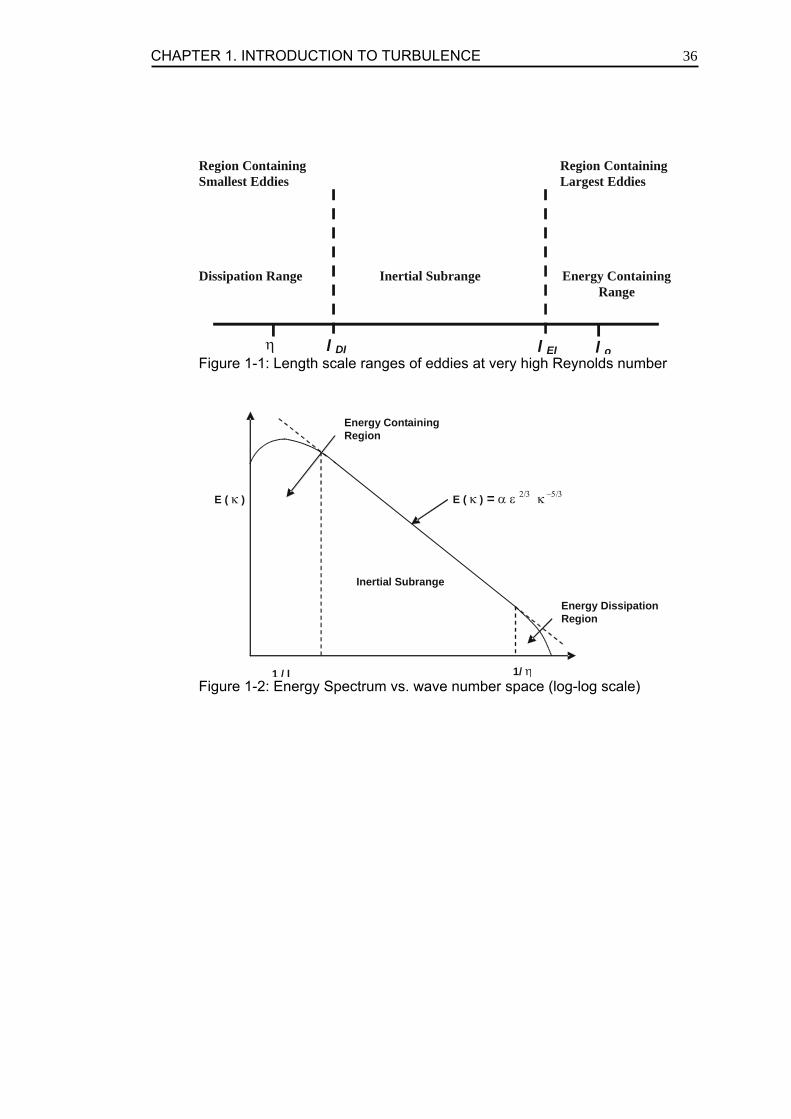
DIl and EIl ( EI DIl l l> > ). All this information can be summed up by Figure 1-1. The right most region in Figure 1-1 is the region which contains the largest eddies whose length scales vary from EIl l L< < , where L is the characteristic length of the flow domain. This is the region in which bulk of the energy is present which explains the name Energy Containing range. The centre region, the Inertial sub range is the region in which motions are dominated by inertial effects as indicated by the name. In this region the viscous effects are negligible. The last region, the dissipation region is where eddies vanish, dissipating all their energy due to effective viscous forces. The energy spectrum curve (see Figure 1-2) shows the energy contained in eddies of various length scales in the flow domain. The graph can be interpreted as a figure showing the amount of energy contained by eddies of various frequencies at a particular instant. The centre region in Figure 1-2 is the inertial sub-range where only dissipation and wave number (κ ) play an important part. For this region based on dimensional analysis one obtains the straight line energy profile bearing the following relationship
2/3 5/3( )E κ αε κ −= (1.8)
where α is a constant and 2lπκ = .
1.2). VELOCITY PROFILES IN THE NEAR WALL REGION Near the solid walls in a flow domain there are essentially two distinct regions, the inner layer and the outer layer. The Inner layer itself comprises of a viscous sublayer and a buffer layer. Inside this viscous sublayer the laminar shear stress lamτ is constant and is equal to the wall shear stress wτ , whereas the turbulent shear stress turτ decreases as Y3 where Y is the distance to the wall. Defining the friction velocity as * 1/ 2( / )wu τ ρ= , the thickness of the viscous sublayer can be expressed as
*
5Sub
vu
δ = (1.9)
where */v u is the viscous length scale. The mean velocity is now read as u Y+ += (1.10)
where * *( ) / , /Y u y v u u u+ += = , ρ is the density and wτ is the wall shear stress. The outer layer on the other hand is dominated by the turbulent or Reynolds stresses with considerable mixing taking place. The flow is random and eddies are present inside the flow with the viscous effects not having much part to play. For the outer layer for 30Y + > , the log law is valid which is defined as
CHAPTER 1. INTRODUCTION TO TURBULENCE 26
1 (ln ) 5.5u Yk
+ += + (1.11)
where k is the Von-Karman constant ( 0.41k ≈ ). To match both layers (inner and outer layers) a Buffer layer is used between 5 30Y +< < .
1.3). TURBULENT FLOW HANDLING There are two different approaches to predict turbulent flows, Statistical approach and Non-Statistical approaches. Statistical approaches will be discussed (Reynolds-Averaged Navier-Stokes) here. The Non Statistical approach will be discussed in the following chapter of this report. As previously stated turbulent flows vary randomly both in time and space, it is due to this variation that turbulent flows cannot be simply handled like laminar flows. The flows are still described by Navier Stokes equations but with additional unknowns (for the case of RANS). Due to the non-linearity extra unknowns arise for which statistical methods rather than deterministic methods have to be studied. This approach is discussed next. In a statistical approach ensemble averaging is carried out to separate mean quantities from fluctuating parts. While averaging the basic equations of motion, correlations involving fluctuating velocities appear. These are additional unknowns for which no equation can be derived without again introducing additional unknowns. This is known as the closure problem of turbulence. To solve this problem closure models are used so that we get additional relations between the correlations and mean quantities. These closure models generally work well for simple flows but become less and less accurate with an increase in the complexity of flow geometry. Despite this fact they are still widely popular in industry due to their lesser computational resource requirement. If u is any instantaneous quantity then it can be decomposed into two parts, the ensemble averaged component u and the fluctuating component u′
u u u′= + (1.12) The momentum equation for the ith component of velocity vector reads as
( )( ) i j ji i
j i j j i
u u uu upt x x x x x
ρρ µ⎡ ⎤⎛ ⎞∂ ∂∂ ∂∂ ∂
+ = − + +⎢ ⎥⎜ ⎟⎜ ⎟∂ ∂ ∂ ∂ ∂ ∂⎢ ⎥⎝ ⎠⎣ ⎦ (1.13)
where ρ is density and µ is the viscosity. Decomposing the variables of this equation into average and fluctuating parts, and then applying ensemble averaging gives us the following equation.
( ) ( )( ) i ji j i ji
j i j j i ji
u u u uu p u ut x x x x x x
ρρ µ ρ⎡ ⎤⎛ ⎞ ′ ′∂ ∂∂ ∂ ∂ ∂ ∂
+ = − + + −⎢ ⎥⎜ ⎟⎜ ⎟∂ ∂ ∂ ∂ ∂ ∂ ∂⎢ ⎥⎝ ⎠⎣ ⎦ (1.14)
This new equation has an additional unknown term when written in tensor form. For a 3-D case this tensor term expands into nine unknown terms (with symmetry these nine terms reduce to six). These unknown terms i ju u′ ′ , called Reynolds stress terms, are related not only to fluid physical properties but
CHAPTER 1. INTRODUCTION TO TURBULENCE 27
also to local flow conditions. However, no further physical laws are available to resolve them. The total stress is then read as
Turbulent Stress
Laminar Stress
( )jiij i j
j i
uu u ux x
τ µ ρ⎛ ⎞∂∂ ′ ′= + −⎜ ⎟⎜ ⎟∂ ∂⎝ ⎠
(1.15)
To calculate turbulent kinetic energy we simply add the Reynolds normal stresses together as shown below
( )12tK u u v v w w′ ′ ′ ′ ′ ′= + + (1.16)
or in tensor form using Einstein summation notation we may write the sum as
( )12t i iK u u′ ′= (1.17)
The turbulence intensity on the other hand is the root mean square value of fluctuating velocities, referred to characteristic mean flow velocity (say 0U )
0 0 0
, , x y zu u v v w wI I IU U U
⎛ ⎞ ⎛ ⎞ ⎛ ⎞′ ′ ′ ′ ′ ′⎜ ⎟ ⎜ ⎟ ⎜ ⎟= = =⎜ ⎟ ⎜ ⎟ ⎜ ⎟⎝ ⎠ ⎝ ⎠ ⎝ ⎠
(1.18)
The total turbulence intensity is sometimes also defined as
0
23
tKIU
⎛ ⎞= ⎜ ⎟
⎝ ⎠ (1.19)
1.4). EDDY VISCOSITY AND MIXING LENGTH THEORY The turbulent shear stress for a special case can be represented by the eddy viscosity approach based upon the Boussinesq hypothesis which reads as
tur tuu vy
τ ρ µ⎛ ⎞∂′ ′= − = ⎜ ⎟∂⎝ ⎠
(1.20)
where tµ is the eddy viscosity. Two important things that need to be kept in mind at this point are that tµ is not a fluid property, instead it depends upon the geometry and the turbulent eddies present in the flow. Second a positive
correlation exists between turτ and uy
∂∂
. Prandtl (1925) proposed that
turbulent fluctuations can be related to a length scale and velocity gradient by
1 2, u vu l v ly y
⎛ ⎞ ⎛ ⎞∂ ∂′ ′= =⎜ ⎟ ⎜ ⎟∂ ∂⎝ ⎠ ⎝ ⎠ (1.21)
where 1l and 2l are mixing lengths and they represent some mean eddy size much larger than the fluids mean free path. If we compare the eddy viscosity approach with mixing length approach we get the mixing length model.
2t m
uly
µ ρ ∂=
∂ (1.22)
The mixing length parameter ml is as difficult to calculate as the Reynolds stresses. This is due to the fact that the mixing length is not constant throughout the domain. Prandtl and Von-Karman estimated that
CHAPTER 1. INTRODUCTION TO TURBULENCE 28
2 viscous sublayer buffer layer
outer layer
l yl kyl const
===
(1.23)
Van Driest (1956) added a damping function for the buffer layer which reads as
1 expbuffYl kyA
+
+
⎡ ⎤⎛ ⎞−= −⎢ ⎥⎜ ⎟
⎝ ⎠⎣ ⎦ (1.24)
Where A+ depends upon the flow conditions such as pressure gradient, wall roughness etc. For a flat plate its value is 26. In some cases eddy viscosity is directly computed using a model by Spalding (1961)
2
12
kB Zt
Zke e Zµ µ − ⎡ ⎤= − − −⎢ ⎥
⎣ ⎦ (1.25)
where Z ku+= .
1.5). TURBULENCE MODELLING In the statistical approach a number of models have been devised to date which shows the difficulty of justifying a fully satisfactory closure. These range from Algebraic models to Reynolds stress models. Perhaps the easiest model to apply is the Zero equation model which does not have any extra differential equations and is actually the mixing length model by Prandtl (1925) (as discussed in previous section), though some more recent versions are also available such as Baldwin-Lomax (1978). There are two broad categories of turbulence models, first order closure models (linear eddy viscosity models) and second order closure models (non linear eddy viscosity models). Zero equation models, one equation models and most of the two equation models are all linear eddy viscosity models. Spalart and Allmaras (1994) use a relatively simple one equation model which solves a modelled transport equation for the turbulent viscosity. This transport equation is based on dimensional analysis and empiricism. The model is supposed to be a local one hence the equation at one point in flow domain depends rather weakly upon the solution at other locations. This makes the model quite robust and easy to apply for any sort of structured or unstructured grids. The model was mainly devised for aerospace applications involving wall bounded flows but has also proved to be quite reliable for boundary layers subjected to adverse pressure gradients. In its original form the Spalart-Allmaras model is a low Reynolds number model and hence requires the viscous dominated region of the boundary layer to be properly resolved. The more advanced breed of models such as eddy viscosity models have become widely popular in the recent past. The linear eddy viscosity models such as widely used k ε− (Launder and Spalding, 1972) and k ω− (Wilcox, 1988) models are based on Boussinesq hypothesis where the underlying
CHAPTER 1. INTRODUCTION TO TURBULENCE 29
assumption is that of isotropic turbulence. The k ε− model solves the kinetic energy and dissipation transport equations in addition to the Navier-Stokes equations whereas the k ω− model solves kinetic energy and vorticity transport equations. The second moment closure models often called the Reynolds Stress models are a relatively newer generation models which are much more complex yet accurate than the zero, one or two equation models. In Reynolds stress models transport equations for each of the terms of the Reynolds stress tensor are solved. An additional scale determining equation for ε is also solved. This means that for a 3-D simulation seven additional equations are now solved. The justification for use of such a computationally expensive model only exists for flows with high anisotropy of turbulence such as stress driven secondary flows, highly swirling flows and flows with buoyancy effects.
1.6). REYNOLDS ENSEMBLE AVERAGING In Reynolds ensemble averaging the solution variables of the Navier-Stokes equations are decomposed into mean and fluctuating parts
i i iu u u′= + (1.26) where iu , iu and iu′ are the instantaneous, mean and fluctuating components respectively. The scalar quantities such as pressure are also decomposed on the same principle.
p p p′= + (1.27) The incompressible Navier-Stokes equation reads
21i i i
jj i j j
u u upu vt u x x xρ
∂ ∂ ∂∂+ = − +
∂ ∂ ∂ ∂ ∂ (1.28)
Inserting the decomposition from equation (1.26) and (1.27) into equation (1.28) gives
( )2( ) ( ) ( )1 ( )i i i i i i
j jj i j j
u u u u u up pu u vt x x x xρ
′ ′ ′′∂ + ∂ + ∂ +∂ +′+ + = − +∂ ∂ ∂ ∂ ∂
(1.29)
Expanding equation (1.29), taking time averaging, ignoring the mean of the fluctuating quantities and keeping the mean of mean quantities gives
21j ii i i
jj j i j j
u uu u upu vt x x x x xρ
′ ′∂∂ ∂ ∂∂+ + = − +
∂ ∂ ∂ ∂ ∂ ∂ (1.30)
the third term on the left hand side of equation (1.30) can now be further modified as
j i j i i j
j j j
u u u u u ux x x
′ ′ ′ ′ ′ ′∂ ∂ ∂= −
∂ ∂ ∂ (1.31)
where the 2nd term on the right hand side of equation (1.31) can be dropped out for an incompressible case ( / 0j ju x∂ ∂ = ). Thus the final Reynolds Averaged Navier-Stokes equations become
21 i ji i i
jj i j j j
u uu u upu vt x x x x xρ
′ ′∂∂ ∂ ∂∂+ = − + −
∂ ∂ ∂ ∂ ∂ ∂ (1.32)
CHAPTER 1. INTRODUCTION TO TURBULENCE 30
where the quantities with over-bar are mean (ensemble averaged) quantities. The last term in equation (1.32) are the Reynolds stresses which need to be modelled for closure of RANS equations.
1.7). REYNOLDS AVERAGED NAVIER-STOKES MODELS
1.7.1). k ε− MODEL The standard k ε− model is the simplest and most complete two equation model. The ease of use and comparatively lower computational cost has made this model the workhorse of the CFD industry. This model was originally presented by Launder and Spalding (1972) although a lot of modified versions now exist. The standard k ε− model is a high Reynolds number model which solves separate transport equations for k and ε . The transport equation for k is given as
( )i Tk
j j k j
ku vk kv Pt x x x
εσ
⎡ ⎤∂ ⎛ ⎞∂ ∂ ∂+ = + + −⎢ ⎥⎜ ⎟∂ ∂ ∂ ∂⎢ ⎥⎝ ⎠⎣ ⎦
(1.33)
and the transport equation for ε is given as
( ) 2
1 2i T
kj j j
u vv c P ct x x x k kε ε
ε
εε ε ε εσ
⎡ ⎤∂ ⎛ ⎞∂ ∂ ∂+ = + + −⎢ ⎥⎜ ⎟∂ ∂ ∂ ∂⎢ ⎥⎝ ⎠⎣ ⎦
(1.34)
in equations (1.33) and (1.34) the production is given as
ik i j
j
uP u ux
∂′ ′= −∂
(1.35)
in conjunction with Boussinesq hypothesis equation (1.35) becomes
1 2 , where the strain rate tensor 2
ik i j
j
jiT ij ij ij
j i
uP u ux
uuv S S Sx x
∂′ ′= −∂
⎛ ⎞∂∂= = +⎜ ⎟⎜ ⎟∂ ∂⎝ ⎠
(1.36)
The turbulent viscosity for this model is approximated as
2
Tkv cµ ε
= (1.37)
where kσ , εσ , cµ , 1cε , and 2cε are all model coefficients given in Table 1-2.
1.7.2). RNG k ε− MODEL The renormalization group theory RNG k ε− model is essentially based on the standard k ε− model but with slight modifications. The ε equation now contains an additional source term which accounts for the improvement of the modelling of rapidly strained flows. The additional source term in the ε equation is
32
33
4
3
1
1c
fc fc
c f k
µ
ε
ε⎛ ⎞
−⎜ ⎟⎝ ⎠
+ (1.38)
CHAPTER 1. INTRODUCTION TO TURBULENCE 31
where ( )/f S k ε= and 2 ij ijS S S= . The model constants are also slightly modified and are given in Table 1-3. The ε equation can now be written as
( ) 2 2
1 2 3
2
2 3 ............................................... ( )
..........................................
i Tk
j j j
u vv c P c ct x x x k k k
c ck
ε ε εε
ε ε
εε ε ε ε εσ
ε
⎡ ⎤∂ ⎛ ⎞∂ ∂ ∂+ = + + − −⎢ ⎥⎜ ⎟∂ ∂ ∂ ∂⎢ ⎥⎝ ⎠⎣ ⎦
= − +
=2
*..... ckε
ε−
(1.39)
where the last two terms can now be combined together ( * 2 3c c cε ε ε= + ). Equation (1.38) is effectively responsible for handling a wide variety of flows. For the outer layer for example the term 3f c< in Equation (1.38), thus 3cε makes a positive contribution to 2cε . This makes the model coefficient *c
ε
higher than 1.68 and hence the model becomes less dissipative. However, inside the log-layer the model coefficient contributes enough to make the value of coefficient *cε equal to approximately 2.0 which is close to the value of 2cε in the standard k ε− model hence behaving in a similar fashion. For the viscous sub-layer the value of 3f c> thus 3cε becomes negative and the value of *cε becomes reduced. This means a less destruction of dissipation, thereby increasing the total dissipation in near wall regions, reducing k and hence effective viscosity. This as a whole makes the RNG model work better for rapidly strained flows where it yields a lower turbulent viscosity than the standard k ε− model. However, there are several other models with similar corrections for rapid strains such as MSST, V2F and non-linear eddy viscosity models.
1.7.3). k ω− MODEL The standard k ω− model was presented by Wilcox (1988) and over the years has become a widely popular model. The model consists of transport equation for k given by
( )i Tk
j j k j
ku vk kv Pt x x x
εσ
⎡ ⎤∂ ⎛ ⎞∂ ∂ ∂+ = + + −⎢ ⎥⎜ ⎟∂ ∂ ∂ ∂⎢ ⎥⎝ ⎠⎣ ⎦
(1.40)
and a transport equation for ω which is defined as rate of dissipation per unit turbulent kinetic energy and is given as
( ) 2i Tk
j j j T
u vv Pt x x x vω
ωω ω α βωσ
⎡ ⎤∂ ⎛ ⎞∂ ∂ ∂+ = + + −⎢ ⎥⎜ ⎟∂ ∂ ∂ ∂⎢ ⎥⎝ ⎠⎣ ⎦
(1.41)
where the turbulent viscosity and dissipation of k are now defined as
* * and Tkv kα ε β ωω
= = (1.42)
and the model coefficients are given in Table 1-4.
CHAPTER 1. INTRODUCTION TO TURBULENCE 32
1.7.4). MSST MODEL The Menter’s Shear Stress Transport (MSST) model was presented by Menter (1994) as a blend of the standard k ε− and k ω− models. The model effectively switches from k ω− model in the near wall region to k ε− in the far field. This is achieved by use of a blending function which turns to 1 in near wall regions and to zero in far field. The model coefficients are also modified and are based on functions which are related to wall distance instead of constant values.
( )i Tk
j j k j
ku vk kv Pt x x x
εσ
⎡ ⎤∂ ⎛ ⎞∂ ∂ ∂+ = + + −⎢ ⎥⎜ ⎟∂ ∂ ∂ ∂⎢ ⎥⎝ ⎠⎣ ⎦
(1.43)
( ) 2i Tk
j j j T
u vv P St x x x v ω
ω
ωω ω α βωσ
⎡ ⎤∂ ⎛ ⎞∂ ∂ ∂+ = + + − +⎢ ⎥⎜ ⎟∂ ∂ ∂ ∂⎢ ⎥⎝ ⎠⎣ ⎦
(1.44)
where Sω is the additional source term and is known as the cross-diffusion term expressed as
( )11.71 1
j j
kS Fx xω
ωω
∂ ∂= −
∂ ∂ (1.45)
the model constants are also not constants anymore and are flow dependent variables based on flow gradients and wall distances and are expressed as shown in Table 1-5 where ( )W curl vorticity= , 1F and 2F are given as
4
1 * 22
500 2tanh min max , ,max ,0n n
nj j
k kFd d kd
x x
µ ωβ ω ρω ω
⎛ ⎞⎡ ⎤⎜ ⎟⎢ ⎥
⎛ ⎞⎜ ⎟⎢ ⎥= ⎜ ⎟⎜ ⎟⎢ ⎥⎜ ⎟ ⎛ ⎞∂ ∂⎝ ⎠⎜ ⎟⎢ ⎥⎜ ⎟⎜ ⎟⎜ ⎟⎢ ⎥∂ ∂⎝ ⎠⎣ ⎦⎝ ⎠
2
2 *
2 500tanh max ,n n
kFd d
µβ ω ρω
⎡ ⎤⎛ ⎞= ⎢ ⎥⎜ ⎟⎜ ⎟⎢ ⎥⎝ ⎠⎣ ⎦
where nd is the distance from the solid wall. Through the sensitivity to W the MSST model reduces viscosity in the presence of velocity and high shear thus having a similar behavior to the RNG k ε− model.
1.7.5). SSG REYNOLDS STRESS MODEL The Speziale Sarkar Gatski (1991) Reynolds stress model is one of the most computationally expensive RANS models. The model is not based on isotropic eddy-viscosity hypothesis and in addition to the transport equation for the dissipation it solves six additional equations for the stress terms. The transport equation for dissipation is given as
( ) 2
1 2i T
kj j j
u vv c P ct x x x k kε ε
ε
εε ε ε εσ
⎡ ⎤∂ ⎛ ⎞∂ ∂ ∂+ = + + −⎢ ⎥⎜ ⎟∂ ∂ ∂ ∂⎢ ⎥⎝ ⎠⎣ ⎦
(1.46)
where the turbulent viscosity is given as
CHAPTER 1. INTRODUCTION TO TURBULENCE 33
Tv c kµ τ= (1.47) and the turbulent time scale is given as
kτε
= (1.48)
The model constants for equations (1.46) to (1.48) are given in Table 1-6. For this model the production kP is given as
12
ik ii i j
j
uP P u ux
∂′ ′= = −∂
(1.49)
The transport equation for the Reynolds stresses is given as
i j k i j v T Pij ij ij ij ij ij
k
u u u u uP D D D
t xφ ε
′ ′ ′ ′∂ ∂+ = − + − + − −
∂ ∂ (1.50)
where the terms on the right hand side are given as
Stress Production j iij i k j k
k k
u uP u u u ux x
∂ ∂′ ′ ′ ′= +∂ ∂
(1.51)
ijPressure-Strain ji
j i
uuPx x
φρ
⎛ ⎞′∂′∂= +⎜ ⎟⎜ ⎟∂ ∂⎝ ⎠
(1.52)
Dissipation 2 jiij
k k
uuvx x
ε′∂′∂
=∂ ∂
(1.53)
Molecular Diffusion i jvij
k k
u uD v
x x
⎛ ⎞′ ′∂∂= ⎜ ⎟⎜ ⎟∂ ∂⎝ ⎠
(1.54)
Turbulent Diffusion Tij i j kD u u u′ ′ ′= (1.55)
( )Pressure Diffusion Pij i jk j ik
PD u uδ δρ
′ ′= + (1.56)
The pressure-strain term ( ijφ ) is broken up into a slow part ( ij,1φ ) and a rapid part ( ij,2φ ) which are modelled as
ij,1 1 213S ij S ik kj mn nm ijc b c b b b bφ ε ε δ⎛ ⎞= − − −⎜ ⎟
⎝ ⎠ (1.57)
( )
ij,2 1
2 3 4
23
2
R ik jk jk ik kl kl ij
R ik jk jk ik R ij R k ij
c k b S b S b S
c k b b c kS c P b
φ δ⎛ ⎞= − + −⎜ ⎟⎝ ⎠
+ Ω + Ω + + (1.58)
where 12 3
ijij ijb
kτ
δ⎛ ⎞
= −⎜ ⎟⎝ ⎠
, 12
jiij
j i
uuSx x
⎛ ⎞∂∂= +⎜ ⎟⎜ ⎟∂ ∂⎝ ⎠
and 12
jiij
j i
uux x
⎛ ⎞∂∂Ω = −⎜ ⎟⎜ ⎟∂ ∂⎝ ⎠
CHAPTER 1. INTRODUCTION TO TURBULENCE 34
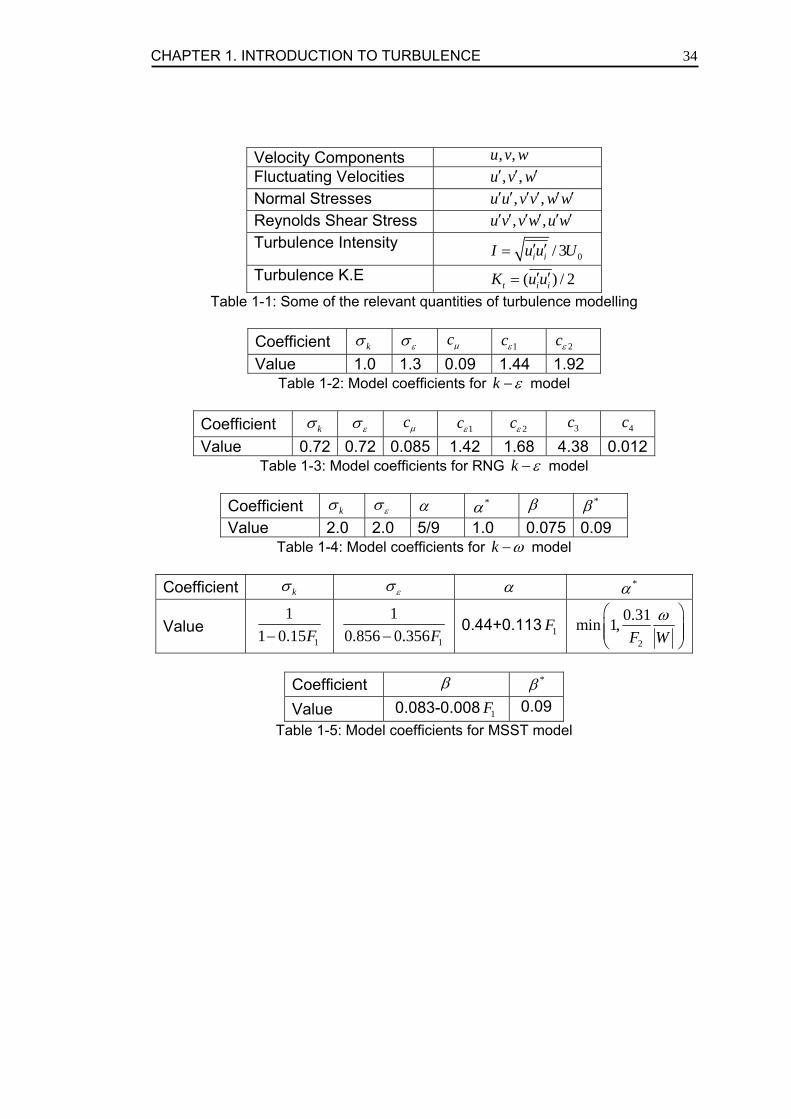
Velocity Components , ,u v w Fluctuating Velocities , ,u v w′ ′ ′ Normal Stresses , ,u u v v w w′ ′ ′ ′ ′ ′ Reynolds Shear Stress , ,u v v w u w′ ′ ′ ′ ′ ′ Turbulence Intensity
0/ 3i iI u u U′ ′= Turbulence K.E ( ) / 2t i iK u u′ ′=
Table 1-1: Some of the relevant quantities of turbulence modelling
Coefficient kσ εσ cµ 1cε 2cε Value 1.0 1.3 0.09 1.44 1.92
Table 1-2: Model coefficients for k ε− model
Coefficient kσ εσ cµ 1cε 2cε 3c 4c Value 0.72 0.72 0.085 1.42 1.68 4.38 0.012
Table 1-3: Model coefficients for RNG k ε− model
Coefficient kσ εσ α *α β *β Value 2.0 2.0 5/9 1.0 0.075 0.09
Table 1-4: Model coefficients for k ω− model
Coefficient kσ εσ α *α
Value 1
11 0.15F−
1
10.856 0.356F−
0.44+0.113 1F 2
0.31min 1,F W
ω⎛ ⎞⎜ ⎟⎜ ⎟⎝ ⎠
Coefficient β *β Value 0.083-0.008 1F 0.09
Table 1-5: Model coefficients for MSST model
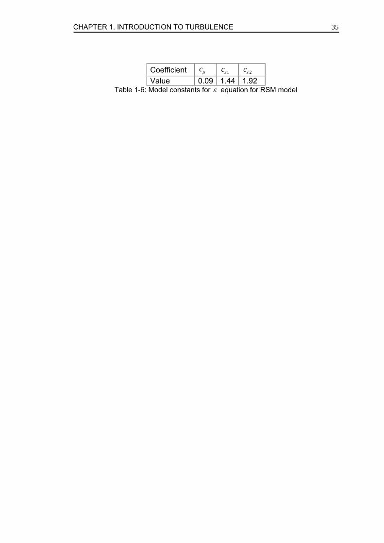
CHAPTER 1. INTRODUCTION TO TURBULENCE 35
Coefficient cµ 1cε 2cε Value 0.09 1.44 1.92
Table 1-6: Model constants for ε equation for RSM model
CHAPTER 1. INTRODUCTION TO TURBULENCE 36
Dissipation Range Inertial Subrange Energy Containing Range
Region Containing Smallest Eddies
Region Containing Largest Eddies
η l ol DI l EI Figure 1-1: Length scale ranges of eddies at very high Reynolds number
Inertial Subrange
Energy DissipationRegion
Energy Containing Region
E ( κ ) = α ε 2/3 κ −5/3 E ( κ )
1 / l 1/ η Figure 1-2: Energy Spectrum vs. wave number space (log-log scale)
CHAPTER 1. INTRODUCTION TO TURBULENCE 37
BIBLIOGRAPHY Baldwin, B. S., Lomax, H. 1978. Thin layer approximation and algebraic model for separated turbulent flow. AIAA paper 78-257. Batchelor, G. K. 1967. An introduction to fluid dynamics. Cambridge university press. Library of Congress catalogue card number 67-21953. Hinze, J. O. 1975. Turbulence. 2nd edition. McGraw-Hill printing. ISBN 0-07-029037-7. Kolmogorov, A. N. 1941. Dissipation of energy in locally isotropic turbulence. Dokl. Akad. Nauk SSSR 32. 19-21. Launder, B. E., Spalding, D. B. 1972. Lectures in mathematical models of turbulence. Academic Press, London, England. Menter, F. R. 1994. Two-Equation eddy-viscosity turbulence models for engineering applications. AIAA 32(8), 1598-1605. Munson, B. R., Young, D. F., Okiishi, T. H. 1994. Fundamentals of fluid mechanics. 2nd edition. John Wiley & Sons, Inc. ISBN 0-471-57958-0. Panton, R. L. 1984. Incompressible Flow. John Wiley & Sons, Inc. ISBN 0-471-89765-5. Pope, S. B. 2000. Turbulent Flows. Cambridge university press. ISBN 0-521-59125-2. Prandtl, L. 1925. Math. Mech., Vol. 5, 136-139. Richardson, L. F. 1922. Weather prediction by numerical process. Cambridge university press. Spalart, P. R. 1988. Direct simulation of a turbulent boundary layer up to Reφ=1400. J. Fluid Mech. Vol 187. 61-98. Schlichting, H. 1979. Boundary layer theory. 7th edition. McGraw-Hill printing. ISBN 0-07-055334-3. Spalding, D. B. 1961. A single formula for the law of the wall. J. Applied Mech. Vol 28. 455-457. Speziale, C. G., Sarkar, S., Gatski, T. B. 1991. Modelling the pressure-strain correlation of turbulence: an invariant dynamical systems approach. J. Fluid Mech. Vol 227. 245-272.
CHAPTER 1. INTRODUCTION TO TURBULENCE 38
White, F. M. 1991. Viscous fluid flow. 2nd edition. McGraw-Hill printing. ISBN 0-07-069712-4. Wilcox, D. C. 1988. Reassessment of the scale determining equation for advanced turbulence models. AIAA J. Vol 26. No 11. 1299-1310.
CHAPTER 2. NON-STATISTICAL APPROACHES 39
Chapter 2 . NON-STATISTICAL APPROACHES
2.1). DIRECT NUMERICAL SIMULATION The most straight-forward approach in solving turbulent flow problems is the Direct Numerical Simulation (DNS) approach in which no modelling assumptions are used. The main assumption in DNS is that the grid is fine enough to capture or resolve all the scales of motion (from largest scales to the smallest Kolmogorov scales). Since DNS has no modelling assumptions, i.e. with governing equations being discretized directly, the results have little or no approximation errors, provided the numerical method is very accurate. With fine enough mesh and higher order accurate numerical schemes the DNS results have a remarkable comparison with experimental results. Another advantage of DNS is that it gives not only the averaged fields but also the instantaneous fields, thus a time dependent solution of the Navier Stokes equations is obtained allowing the capture of quantities which are sometimes even difficult to measure by experiments. There are two limitations in the application of DNS; the high computational cost and need for higher order accurate discretization techniques. The added computational requirement is due to the fact that the grid has to resolve all the turbulent scales of motion from largest macroscopic structures down to the Kolmogorov scales. This puts a strong restriction on the Reynolds number of the flow being computed. As the Reynolds number becomes higher and higher the turbulent scales of motion become smaller and smaller, hence the grid requirement becomes even stricter. Even with modern super computers the most complex of flows with very high Reynolds numbers can not be solved. As shown by equation (1.5) the DNS grid requirement for 1-D is
3/ 4ReLη
≈ (2.1)
where L is the characteristic length scale (or the length scale of the largest eddy), η is the Kolmogorov scale and Re is the Reynolds number referenced to the integral scale of motion. Thus for a 3-D case the grid requirement becomes
9/ 4ReN = (2.2)
CHAPTER 2. NON-STATISTICAL APPROACHES 40
where N is the number of grid cells. We can see that for very high Reynolds number flows even modern day super computers fail. That is not all, with the time scale of smallest eddies also dictating the maximum time step allowed, the computational cost becomes even higher. In wall bounded flows the computational cost becomes yet even higher. The second problem with the practical application of DNS is that it requires higher order accurate schemes. This is due to the fact that the dissipation and dispersion errors have to be limited. Although the spectral methods most commonly employed in DNS have little or no dissipation and dispersion errors, their application to complex flow geometries is still very difficult. Handling of boundary conditions with these schemes is also an issue. Even though the first practical application of DNS was back in 1972 by Orszag and Patterson (1972) for decaying isothermal isotropic turbulence, in recent years most of the DNS studies concern simple channel flows with Cartesian grids as we still lack the computational resources to apply DNS to complex flows with high Reynolds numbers.
2.2). LARGE EDDY SIMULATION Large Eddy Simulation (LES) is the process in which instead of modelling everything like RANS we apply a filtering process and separate large eddies from smaller ones. Based on Kolmogorov principles the smaller scales of motion are universal and isotropic and hence can be modelled, whereas the larger scales which depend on boundary and flow conditions are solved like DNS. In LES the filtering is based on cell volume size. Imagine a computational grid with a certain number of cells in it. Now if the grid becomes coarser and coarser our filter becomes larger and lager meaning less things to solve and more to model (approaching RANS). Conversely if the grid becomes finer and finer the filter becomes smaller and smaller meaning more things to solve and less to model (approaching DNS). Because LES is a compromise between DNS and RANS, it is more accurate than RANS and computationally less expensive when compared to DNS. For this reason LES is becoming widely popular in academia, and even in industry in recent years. Geometries being simulated by LES vary from simple channel flows to complex engineering flows such as tube bundles and power-plant thermohydraulic applications. LES like DNS has another advantage over RANS; it can predict the time dependent behaviour of Navier Stokes equations so we can see the development of solution both in time and space.
2.3). FILTERING IN LES Filtering is applied to introduce the separation of resolved scales from unresolved ones. Suppose that the unfiltered function is ( )f x′ , then its filtered component f and sub grid scale fluctuating part ( )f x′ are defined as
CHAPTER 2. NON-STATISTICAL APPROACHES 41
( ) ( ) ( , ) '( ) ( ) ( )D
f x f x G x x dx f x f x f x′ ′ ′= = −∫ (2.3)
where ( , )G x x′ is the filter function, having the following property
( , ) 1G x x dx′ ′ =∫ (2.4)
Note that the filter function ( , )G x x′ depends upon the local position x and the its neighbourhood x′ . The filtering can be interpreted as some kind of local averaging in the neighbourhood of position x′ . When the grid is homogeneous (i.e. constant mesh steps) the filter function only depends on the separation r x x′= − . The filter is often chosen so that it mimics the smoothing effect resulting from discretizing the equations on a grid (for instance interpolation from cell centres to cell faces smoothes the signal). The most commonly used filters are box filter, the Gaussian filter and the sharp spectral cut off filter. The box filter is defined as
1/ if x / 2
( )0 otherwise
G x⎧ ∆ ≤ ∆⎪= ⎨⎪⎩
(2.5)
which means that the filtered value of the signal is now the mean over the interval / 2±∆ . The Gaussian filter function is the Gaussian distribution with mean zero and variance 2 /12∆ . The Gaussian filter is defined as
( )26( ) exp 6 /G x xπ
= − ∆∆
(2.6)
The sharp spectral filter defined as
( )sin /( )
xG x
xππ
∆= (2.7)
The behaviour of box filter in real space is the same as the behaviour of sharp spectral filter in wave number space. It is however, interesting to note that the choice of the filter for an LES is not the only important issue. There are other far more critical issues such as discretization schemes, mesh resolution and subgrid-scale model as pointed out by Germano (1991).
2.3.1). FILTERED NAVIER STOKES EQUATIONS If u is an instantaneous quantity, u the resolved large scale and u′ is the unresolved small scale then the filtered Navier-Stokes equation reads as
2( ) ( )1i ji i
j i j j
u uu up vt x x x xρ
∂∂ ∂∂+ = − +
∂ ∂ ∂ ∂ ∂ (2.8)
breaking the ( )i ju u component as below
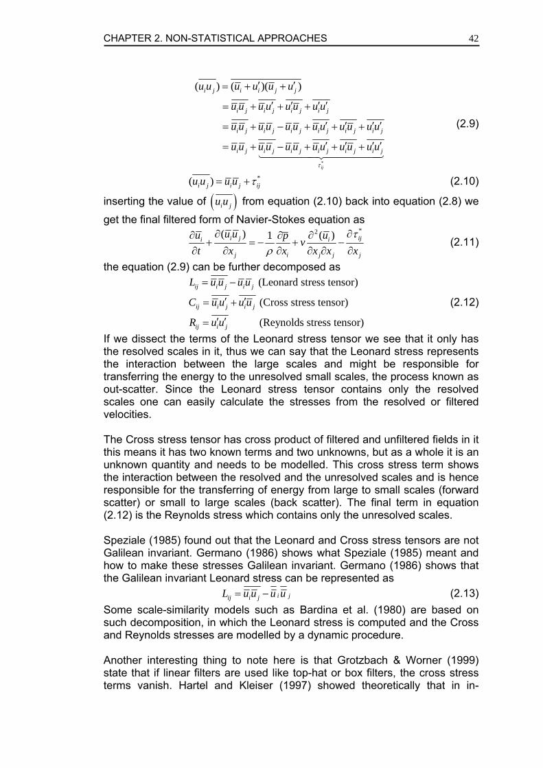
CHAPTER 2. NON-STATISTICAL APPROACHES 42
*
( ) ( )( )
ij
i j i i j j
i j i j i j i j
i j i j i j i j i j i j
i j i j i j i j i j i j
u u u u u u
u u u u u u u u
u u u u u u u u u u u u
u u u u u u u u u u u uτ
′ ′= + +
′ ′ ′ ′= + + +
′ ′ ′ ′= + − + + +
′ ′ ′ ′= + − + + +
(2.9)
*( )i j i j iju u u u τ= + (2.10)
inserting the value of ( )i ju u from equation (2.10) back into equation (2.8) we
get the final filtered form of Navier-Stokes equation as
*2( ) ( )1i j iji i
j i j j j
u uu up vt x x x x x
τρ
∂ ∂∂ ∂∂+ = − + −
∂ ∂ ∂ ∂ ∂ ∂ (2.11)
the equation (2.9) can be further decomposed as
(Leonard stress tensor)
(Cross stress tensor)
(Reynolds stress tensor)
ij i j i j
ij i j i j
ij i j
L u u u u
C u u u u
R u u
= −
′ ′= +
′ ′=
(2.12)
If we dissect the terms of the Leonard stress tensor we see that it only has the resolved scales in it, thus we can say that the Leonard stress represents the interaction between the large scales and might be responsible for transferring the energy to the unresolved small scales, the process known as out-scatter. Since the Leonard stress tensor contains only the resolved scales one can easily calculate the stresses from the resolved or filtered velocities. The Cross stress tensor has cross product of filtered and unfiltered fields in it this means it has two known terms and two unknowns, but as a whole it is an unknown quantity and needs to be modelled. This cross stress term shows the interaction between the resolved and the unresolved scales and is hence responsible for the transferring of energy from large to small scales (forward scatter) or small to large scales (back scatter). The final term in equation (2.12) is the Reynolds stress which contains only the unresolved scales. Speziale (1985) found out that the Leonard and Cross stress tensors are not Galilean invariant. Germano (1986) shows what Speziale (1985) meant and how to make these stresses Galilean invariant. Germano (1986) shows that the Galilean invariant Leonard stress can be represented as
i jij i jL u u u u= − (2.13) Some scale-similarity models such as Bardina et al. (1980) are based on such decomposition, in which the Leonard stress is computed and the Cross and Reynolds stresses are modelled by a dynamic procedure. Another interesting thing to note here is that Grotzbach & Worner (1999) state that if linear filters are used like top-hat or box filters, the cross stress terms vanish. Hartel and Kleiser (1997) showed theoretically that in in-
CHAPTER 2. NON-STATISTICAL APPROACHES 43
homogeneous flows near walls the energy transfer between resolved and unresolved scales is independent of the filter used. One last thing to note here is that non-homogeneous meshes will correspond to variable filter width. The filter then depends on the local position and
( , )G x x′ must be used instead of ( )G x x′ − . It follows that filtering and spatial differentiation no longer commute and the Filtered Navier Stokes equations are then more complex than (2.8). The error scales with the gradient of the filter width ( ∆ ), hence the cell size should only increase gradually but this is difficult to control with the unstructured grids considered later in this thesis. There are many issues around filtering and a consensus is far from being reached, but the present work will focus mainly on applications. One can say that the errors due to filter commutation errors, explicit versus implicit filtering, numerical scheme errors, etc. all decrease when the mesh is refined, together with errors due to sub-grid scale modelling errors. Although not entirely satisfying, one can establish some confidence in the LES results presented later by checking that these results show little variation when the meshes are refined.
2.4). SUBGRID SCALE MODELLING By filtering we have divided our problem into two main parts; the large scales and the small scales. The large scales are solved by the Navier Stokes equations but the small scales are left to be modelled. Since the small scales are isotropic and universal we can use a modelling approach. These models are known as the Subgrid scale models (SGS). The idea behind subgrid scale modelling is more or less the same as behind RANS. There are a variety of SGS models, the oldest one being the Smagorinsky model presented in 1963. This model is based on the concept of eddy viscosity and is hence classified as an Eddy viscosity model. Other classes of models are scale similarity models, transport models and de-convolution models. Recently some spectral models have also been presented but due to their complexity of application they are not yet very popular. In the next few sections special emphasis will be given to the explanation of the popular Smagorinsky model, the Dynamic Smagorinsky model and the Wall Adapting Local Eddy Viscosity Model (WALE).
2.4.1). EDDY VISCOSITY MODELS Eddy viscosity models are based on the concept that only global effects of SGS terms such as dissipation are important and the local energy events associated with convection and diffusion may be neglected. Another assumption in Eddy viscosity models is that of equilibrium (the rate of production of energy is equal to the rate of dissipation). This is because the small eddies have a much smaller time scale than the large ones so they adjust themselves very rapidly to small perturbations and recover equilibrium
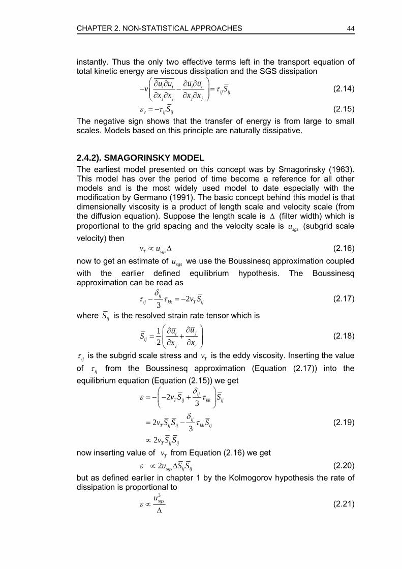
CHAPTER 2. NON-STATISTICAL APPROACHES 44
instantly. Thus the only two effective terms left in the transport equation of total kinetic energy are viscous dissipation and the SGS dissipation
i i i iij ij
j j j j
u u u uv Sx x x x
τ⎛ ⎞∂ ∂ ∂ ∂
− − =⎜ ⎟⎜ ⎟∂ ∂ ∂ ∂⎝ ⎠ (2.14)
v ij ijSε τ= − (2.15) The negative sign shows that the transfer of energy is from large to small scales. Models based on this principle are naturally dissipative.
2.4.2). SMAGORINSKY MODEL The earliest model presented on this concept was by Smagorinsky (1963). This model has over the period of time become a reference for all other models and is the most widely used model to date especially with the modification by Germano (1991). The basic concept behind this model is that dimensionally viscosity is a product of length scale and velocity scale (from the diffusion equation). Suppose the length scale is ∆ (filter width) which is proportional to the grid spacing and the velocity scale is sgsu (subgrid scale velocity) then
T sgsv u∝ ∆ (2.16) now to get an estimate of sgsu we use the Boussinesq approximation coupled with the earlier defined equilibrium hypothesis. The Boussinesq approximation can be read as
23ij
ij kk T ijv Sδ
τ τ− = − (2.17)
where ijS is the resolved strain rate tensor which is
12
jiij
j i
uuSx x
⎛ ⎞∂∂= +⎜ ⎟⎜ ⎟∂ ∂⎝ ⎠
(2.18)
ijτ is the subgrid scale stress and Tv is the eddy viscosity. Inserting the value of ijτ from the Boussinesq approximation (Equation (2.17)) into the equilibrium equation (Equation (2.15)) we get
23
23
2
ijT ij kk ij
ijT ij ij kk ij
T ij ij
v S S
v S S S
v S S
δε τ
δτ
⎛ ⎞= − − +⎜ ⎟
⎝ ⎠
= −
∝
(2.19)
now inserting value of Tv from Equation (2.16) we get 2 sgs ij iju S Sε ∝ ∆ (2.20)
but as defined earlier in chapter 1 by the Kolmogorov hypothesis the rate of dissipation is proportional to
3sgsu
ε ∝∆
(2.21)
CHAPTER 2. NON-STATISTICAL APPROACHES 45
thus we can equate equations (2.20) and (2.21) to get an estimate of sgsu
2sgs ij iju S S∝ ∆ (2.22)
by doing so we have estimated a value of sgsu . Now inserting it back in the original equation (2.16) we get an estimate of the eddy viscosity
2 2T ij ijv S S∝ ∆ (2.23) And introducing a proper constant we get
2( )T Sv C S= ∆ (2.24)
where 2 ij ijS S S= and SC is the Smagorinsky constant which was first estimated by Lilly (1967), on the basis of inertial range dynamics given by equation (1.8). The strain rate tensor can be calculated by integrating the dissipation spectrum over the resolved wave number
2/3 5/3( )E κ αε κ −= (2.25)
/
2 2
0
2 ( )S E dπ
κ κ κ∆
= ∫ (2.26)
4/3
2 2/332
S παε ⎛ ⎞= ⎜ ⎟∆⎝ ⎠ (2.27)
if we insert the value of ijτ from the original Boussinesq approximation (equation (2.17)) into the equilibrium law (equation (2.15)) we get
( 2 )
2
sgs ij ij
T ij ij
T ij ij
S
v S S
v S S
ε τ= −
= − −
=
(2.28)
now using the Smagorinsky model (equation (2.24))
2
32
2(( ) )
( )
sgs S ij ij
S
C S S S
C S
ε = ∆
= ∆ (2.29)
inserting the value of S from equation (2.27) into equation (2.29) we get
3/ 24/3
2 2/33( )2sgs SC πε αε
⎛ ⎞⎛ ⎞= ∆ ⎜ ⎟⎜ ⎟⎜ ⎟∆⎝ ⎠⎝ ⎠ (2.30)
with further mathematical manipulation we get
3/ 41 2
3SCπ α
⎛ ⎞≈ ⎜ ⎟⎝ ⎠
(2.31)
For the homogeneous isentropic flow case Lilly (1967) used a value of 1.0α = , with this value he got a universal value of 0.23SC = . Later
experimentations showed this value of SC to be quite high. There are two shortcomings with Smagorinsky model. One of them is the excessive damping of resolved turbulent kinetic energy when SC is used as predicted by Lilly (1967). Furthermore an estimate of a universal constant is very difficult for different flows especially with mean shear flows. The other
CHAPTER 2. NON-STATISTICAL APPROACHES 46
problem with the Smagorinsky model is that it does not account for any backscattering (energy flow from small to large scales) as shown by Piomelli et al. (1991).
2.4.3). DYNAMIC SMAGORINSKY MODEL As stated earlier as well, in mean shear flows it is very difficult to predict a correct value of Smagorinsky constant. To avoid excessive damping Deardoff (1970) used a value of 0.1 for turbulent channel flow and achieved acceptable results. As mentioned earlier, the numerical scheme can also introduce errors of a mainly dissipative nature, in particular when implicit filtering is assumed. The common practice to date is to get an estimate of the natural dissipation of a code by running tests on a homogeneous isotropic turbulence case and then adjusting the Smagorinsky constant accordingly; Addad (2004). Near solid walls the Smagorinsky model needs to be damped by Van-Driest wall damping function to properly reproduce the transition from the purely viscous sublayer to the turbulent Log layer. This is done to force the value of Smagorinsky constant to zero at the wall at the appropriate rate as a function of the wall distance. These rather “ad-hoc” corrections and the inability of the Smagorinsky model to account for the backscatter led Germano et al. (1991) to propose a Dynamic Smagorinsky model. The dynamic model works in a similar fashion to the Smagorinsky model but with an additional test filter. The difference between the test filter and grid filter leads to an estimate of the dynamic Smagorinsky coefficient dynC . The effects of small scales appear in the subgrid-scale stress term as shown by equation (2.10). Recalling that the grid filtered Navier-Stokes equations are
given as *2( ) ( )1i j iji i
j i j j j
u uu up vt x x x x x
τρ
∂ ∂∂ ∂∂+ = − + −
∂ ∂ ∂ ∂ ∂ ∂. Applying the test filter
( ) ( ) ( , )f x f x G x x dx′ ′ ′= ∫ to the filtered Navier-Stokes equations leads to
2( ) 1 ( )i j i iji
j i j j j
Tu u u p uvt x x x x xρ
∂∂ ∂ ∂ ∂+ = − + −
∂ ∂ ∂ ∂ ∂ ∂ (2.32)
where the subgrid-scale stresses read i jij i jT u u u u= − (2.33)
The resolved turbulent stresses ( ijζ ) are representative of the contribution of the Reynolds stresses of the scales which have a length scale bigger than the grid filter and smaller than the test filter
i jij i ju u u uζ = − (2.34) these resolved turbulent stresses are related to the subgrid-scales at resolved and test level by the algebraic relationship given by Germano (1990) as
ij ij ijTζ τ= − (2.35)
CHAPTER 2. NON-STATISTICAL APPROACHES 47
where the terms ijT and ijτ can be approximated by use of equation (2.17) and (2.24) as
2( / 3) 2ij ij kk S ijC S Sτ δ τ− = − ∆ (2.36)
2( / 3) 2 ijij ij kk ST T C S Sδ− = − ∆ (2.37)
where 12
i jij
j i
u uSx x
⎛ ⎞∂ ∂= +⎜ ⎟⎜ ⎟∂ ∂⎝ ⎠
and 2 mn nmS S S= . Now substituting values of ijT
and ijτ from equations (2.36) and (2.37) into equation (2.35) yields
( ) ( )2 22 2ijij S S ijC S S C S Sζ = − ∆ − − ∆ (2.38)
then contracting both sides with ijS results in
( ) ( )2 22 2ijij ij S ij S ij ijS C S S S C S S Sζ = − ∆ − − ∆ (2.39)
from equation (2.39) the value of the Smagorinsky constant SC can in principle be obtained. This is done by computing the tested filtered quantities by external filtering. However, the right hand side of equation (2.39) can become zero making the constant indeterminate and the system ill-conditioned. Germano et al. (1991) implemented this model by doing local averaging in planes parallel to solid walls assuming that SC is a function of only wall normal direction and time. However, this is a broad assumption which still might not be sufficient for general applications. Readers are encouraged to refer to Piomelli et al. (1994) for the application of the dynamic model with localized averaging for rotating channel flow cases. Lilly (1991) proposed a modified version of the dynamic model based on a least square approach where the resolved turbulent stresses ( ijζ ) in equation (2.35) can be represented as
( ) ( )
( )2 2
2 2
(1/ 3) 2 2
2
ij
ijij ij kk S S ij
ijS ij
M
C S S C S S
C S S S S
ζ δ ζ− = − ∆ − − ∆
= −∆ + ∆ (2.40)
(1/ 3) 2ij ij kk S ijC Mζ δ ζ− = (2.41)
where 2 2ijij ijM S S S S= −∆ + ∆ . By defining a least square approach for the
solution of equation (2.41) one gets
1/ 2 1 23ij ij kk S ijQ C Mζ δ ζ= − − (2.42)
taking square of equation (2.42) one gets 2 2 2 2 21 2 44 4
9 3 3ij ij kk S ij ij ij kk ij S ij ij S ij kkQ C M C M C Mζ δ ζ δ ζ ζ ζ δ ζ= + + − − + (2.43)
by only keeping the isotropic terms this equation reduces to 2 2 24 4ij S ij ij S ijQ C M C Mζ ζ= + − (2.44)
CHAPTER 2. NON-STATISTICAL APPROACHES 48
taking the derivation of equation (2.44) and equating it to zero yields the value of SC as
28 4 0S ij ij ijS
Q C M MC
ζ∂= − =
∂ (2.45)
2
12
ij ijS
ij
MC
Mζ⎛ ⎞
= ⎜ ⎟⎜ ⎟⎝ ⎠
(2.46)
the obvious advantage of Lilly’s approach is that the denominator in equation (2.46) hardly vanishes to zero, which would only occur if all the individual terms of ijM go to zero.
2.4.4). WALL-ADAPTING LOCAL EDDY-VISCOSITY MODEL A relatively newer model based on the square of velocity gradient tensor was presented by Nicoud and Ducros (1999). Unlike the Smagorinsky model which is based only on the strain rate gradient the Wall-Adapting Local Eddy Viscosity (WALE) Model is based on true velocity gradients and hence can distinguish between pure strain and rotation rates. A simple way to build an operator is to consider the traceless part of the square of the velocity gradient tensor which is
( ) ( )2 2 21 1&2 3
dij ij ji ij kkg g gδ= + − (2.47)
where iij
j
ugx
∂=
∂ and 2
ij ik kjg g g= . Equation (2.47) can now be written in terms
of strain and rotation rates as
1&3
dij ik kj ik kj ij mn mn mn mnS S S Sδ ⎡ ⎤= + Ω Ω − + Ω Ω⎣ ⎦ (2.48)
by considering incompressibility and making use of the Cayley-Hamilton theorem this becomes
( )2 2 2 2 2 21 2& & 26 3
d dij ij SS S S IV Ω= + Ω Ω + Ω + (2.49)
where 2ij ijS S S= , 2
ij ijΩ = Ω Ω and S ik kj jl liIV S SΩ = Ω Ω . The equation (2.49) can now account for turbulent structures with large strain rates, rotation rates or both. For pure shear flows all the terms will drop out leaving only 12g which
would yield 2 2 2122S S= Ω = and 2 21
2SIV S SΩ = − . This would make the operator
in equation (2.49) as zero, a condition which is true and physical for wall bounded laminar flows. It also signifies the fact that the contribution of shear zones to energy dissipation is far less than that of eddies. For subgrid-scale viscosity modelling the WALE model is finally proposed as
( )
( ) ( )
3/ 2
12 25/ 45/ 2
2
& &( ) ( )
& &
d dij ij
T W W d dij ij ij ij
OPv C COP S S
= ∆ = ∆+
(2.50)
CHAPTER 2. NON-STATISTICAL APPROACHES 49
where WC is the WALE model constant which can be estimated by assuming that the model gives the same ensemble average subgrid kinetic energy dissipation as the Smagorinsky model
( )3/ 21/ 2
2 2
1
2
2 ij ij
W S
ij ij
S SC C
OPS SOP
= (2.51)
The prescribed value of WC can differ from case to case. However, it is seen from simulations (which will be reported in the next few chapters) that the WALE model is not as highly dependent upon the constant as the Smagorinsky model. The operators ( )3/ 2
1 & &d dij ijOP = and
( ) ( )5/ 45/ 2
2 & &d dij ij ij ijOP S S= + are based on physical wall behaviour and
dimensional analysis to yield true Y3 scaling for Tv with correct units of m2/s. Other SGS models such as scale similarity models, transport equation models, subgrid scale heat flux models and higher order spectral models also exist but are not discussed here. Readers may find details about spectral models in Chollet and Lesieur (1981).
2.5). OTHER ASPECTS OF LES Other aspects of LES such as numerics, time stepping, grid resolution and boundary conditions are discussed in details in the succeeding chapters. However, some degree of introduction is provided in this section. For a typical LES the grid resolution requirement is quite high where the implicit filter should lie within the inertial sub-range. This allows the filtering process to capture all the energy containing eddies. However, if the geometry is homogenous in all directions (no solid wall present) then the grid resolution becomes independent of the Reynolds number. But in the presence of solid walls the scenario changes, according to Chapman (1979) the resolution requirement for the outer layer of a growing boundary layer is 0.4Re and for the viscous sub layer this requirement is 1.8Re . To resolve the near wall structures Frohlich and Rodi (2002) recommend that for a typical LES case
2Y +∆ ≈ (wall normal direction), 50 150X +∆ ≈ − (streamwise direction), 15 40Z +∆ ≈ − (spanwise direction). These grid resolution requirements can be
easily met for low to moderate Reynolds number. However, at fairly high Reynolds numbers even LES becomes computationally very expensive much like DNS. Practical solutions then lie in using appropriate wall functions much like in RANS modelling. For the classical Smagorinsky model one has to further use the Van-Driest wall damping function near solid walls to artificially damp the model constant. With LES initial conditions are also equally important. Unrealistic or poor initial conditions can lead to delayed or inadequate flow development. To

CHAPTER 2. NON-STATISTICAL APPROACHES 50
enhance the flow development a number of techniques are utilized. Lee et al. (1992) use a mean velocity profile at inlet with a random noise applied to it. Lund et al. (1998) re-scale the velocity at the outlet and reintroduces it to the inlet. Other techniques involve using the instantaneous results of separate simulations. However, such approaches are by no means perfect and still require further development.
CHAPTER 2. NON-STATISTICAL APPROACHES 51
BIBLIOGRAPHY Addad, Y. 2004. LES of bluff body, mixed and natural convection turbulent flows with unstructured FV codes. PhD Thesis University of Manchester. Anderson, D. A., Tannehill, J. C., Pletcher, R. H. 1984. Computational Fluid Mechanics and Heat Transfer. Hemisphere publishing corporation. ISBN 0-89116-471-5. Provitola, A., Denaro, F., M. 2004. On the application of congruent upwind discretizations for LES. J. Comp. Phys. 194. 329-343. Bardina, J., Ferziger, J. H. and Reynolds, W. C. 1980. Improved subgrid-scale models for large eddy simulation. AIAA J. 80-1357. Boris, J. P., Grinstein, F. F., Oran, E. S., Kolbe, R. L. 1992. New insights into LES. Fluid Dyn. Res. 10, 199-228. Breuer, M., Rodi, W. 1994. LES of turbulent flow through a straight square duct and 1800 bend. Voke, P. et al. (Eds), Direct and LES I. Kluwer Academic Publishers, Dordrecht. 273-285. Chapman, D. R. 1979. Computational aerodynamics development and outlook AIAA J. 17. 1293. Chollet, J. P., Lesieur, M. 1981. Parameterization of small scales of three dimensional isotropic turbulence utilizing spectral closures. J. Atoms. Sci. 38, 2747-2757. Chow, F., K., and Street, R., L. 2002. Modelling unresolved motions in LES of field scale flows. 15th Symposium on Boundary Layers and Turbulence, 15-19 July, 2002, Wageningen, The Netherlands. Deardorff, J. W. 1970. A numerical study of three-dimensional turbulent channel flow at high Reynolds numbers. J. Fluid Mech. Vol 41, 453-480. Frohlich, J., Rodi, W. 2002. Introduction to large eddy simulation of turbulent flows. Closure strategies for turbulent and transitional flows by B. Launder and N. Sandham, Cambridge university press. 267-298. Germano, M. 1986. A proposal for a redefinition of the turbulent stresses in the filtered Navier-Stokes equations. Physical Fluids 29(7). 2323-2324. Germano, M. 1991. Turbulence: The filtering approach. J. Fluid Mech. 238, 326-336.
CHAPTER 2. NON-STATISTICAL APPROACHES 52
Germano, M., Ugo Piomelli, Moin, P. and William, H. Cabot. 1991. A dynamic subgrid-scale eddy viscosity model. Phys. Fluids A. 3(7). 1760-1765. Grotzbach, G. and Worner, M. 1999. Direct numerical and large eddy simulation in nuclear applications. Int. J. Heat Fluid Flow. 20. 222-240. Gullbrand, J. 2001. Explicit filtering and subgrid-scale models in turbulent channel flow. Centre for Turbulent Research, Annual Research Briefs. Hartel, C., Kleiser, L. 1997. Galilean invariance and filtering dependence of near wall grid-scale/subgrid scale interactions in large eddy simulation. Phys. Fluids 9. 473-475. Kravchenko, A. G., Moin, P. 1997. On the effects of numerical errors in large eddy simulation of turbulent flows. J. Comp. Phys. 131. 310-322. Lee, S., Lele, S. K., Moin, P. 1992. Simulation of spatially evolving turbulence and the applicability of Taylor's hypothesis in compressible flow. Phys. Fluids A. (4) 1521. Lilly, D. K. 1967. The representation of small scale turbulence in numerical simulation experiments. Proc. IBM scientific computing symposium on environmental sciences. Yorktown Heights N. Y. 195. Lilly, D. K. 1991. A proposed modification of the Germano subgrid-scale closure method. Phys. Fluids A. 4(3) 633-635. Lund, T. S., Wu, X., Squires, K. D. 1998. Generation of inflow data for spatially-developing boundary layer simulations. J. Comp. Phys. 140. 233. Morinishi, Y., and Kobayashi, T. 1991. Large eddy simulation of complex flow fields. Comp. Fluids. Vol. 19, No. 3/4, pp. 335-346. Nicoud, D., Ducros, F. 1999. Subgrid-scale modelling based on the square of the velocity gradient tensor. Flow Turb. Comb. Vol. 62. 183-200. Oleg, V. Vasilyev, Thomas, S. Lund, and Parviz Moin. 1998. A General Class of Commutative Filters for LES in Complex Geometries. J. Comp. Phys. 146, 82--104. Patankar, S. V. 1980. Numerical heat transfer and fluid flow. McGraw-Hill Book Company. ISBN 0-07-048740-5. Piomelli, U., Cabot, W. H., Moin, P. and Lee, S. 1991. Phys. Fluids A 3. 1766. Piomelli, U., Liu, Junhui. 1994. Large-eddy simulation of rotating channel flows using a localized dynamic model. Phys. Fluids 7 (4). 839-848.

CHAPTER 2. NON-STATISTICAL APPROACHES 53
Pope, S. B. 2000. Turbulent Flows. Cambridge university press. ISBN 0-521-59125-2. Sagaut, P. 1998. Introduction to large scale eddy simulation for incompressible fluid flows. Aerospace Science and Technology, no. 6, 413-414. Smagorinsky, J. 1963. General circulation experiments with the primitive equations. The basic experiment. Monthly weather review Vol 91, page 99. Speziale, C. G. 1985. J. Fluid Mech. Vol 156, 55-62.
CHAPTER 3. NUMERICAL TREATMENT
54
Chapter 3 . NUMERICAL TREATMENT The general transport equation for a control volume in the current solver can be expressed as
1
Rate of change Convection term
1 1
Diffusion term Source terms
( ).
. .
f
j
f f
j j
n
SjV S
n n
S Vj jS S V
d B dV V V dsdt
grad ds q ds q dV
φ
φ φ φ
ρ ρφ
φ
=
= =
+ −
= Γ + +
∑∫ ∫
∑ ∑∫ ∫ ∫ (3.1)
The above equation has four distinct parts; the transient rate of change term, the convection term, the diffusion term and the source term. Each of these terms are discretized and dealt with differently as will be shown in the subsequent sections.
3.1). CELL AND FACE BASE DEFINITIONS
3.1.1). FACE SURFACE VECTORS The control volumes (CV) or cells in the current solver can be of any polyhedral shape with cell surfaces or faces of arbitrary polygonal shapes. To calculate the surface area of such an arbitrary shape the following relation is used
( ) ( )1 1 13
12
n
j i ii
s r r r r−=
⎡ ⎤= − × −⎣ ⎦∑ (3.2)
where js is the surface vector of a face and ir is the position vector of a vertex on that face. This procedure breaks the control volume surface into different triangles thereby calculating their individual areas, summation of which leads to the total face surface vector.
3.1.2). CELL VOLUME The cell volumes are computed by summation of the product of position vector ( jr ) of the cell face centre and the cell face surface vector ( js ) as shown below
CHAPTER 3. NUMERICAL TREATMENT
55
0
1
1 .3
n
P j jj
V r s=
= ∑ (3.3)
This approximation is based on mid-point rule which states that the integral is equal to the product of the integrand at the centre of the domain and the surface or volume of that domain
0 0
js
f. f . or j j P PV
ds s fdV f V≈ ≈∫ ∫ (3.4)
where f is any vector quantity and f is any arbitrary scalar.
3.1.3). CELL AND FACE VALUE CALCULATION To transport the cell centre value to any location in the domain the following second order interpolation based on Taylor expansion is used
0 0 0
( ) ( ) .( )P P Pr grad r rψ ψ ψ= + − (3.5) where ψ is the interpolation variable, r the position vector as already defined and 0P the cell centre location. To calculate the surface integral of a CV, variable values at the cell face centres are required which are computed as
( ) ( ) ( ) ( )0 00
1 1( ) . .2 2j jj
j P P j P j PP Pgrad r r grad r rψ ψ ψ ψ ψ⎡ ⎤= + + − + −⎢ ⎥⎣ ⎦
(3.6)
where subscript 0P is for cell centre locations, jP is for neighbour cell centre location and jr is the position vector for the cell face centre between the two cells (see Figure 3-1). The second term in equation (3.6) takes into account the location of the cell face centre which might not be located on the straight line connecting the two cell centres.
3.1.3). GRADIENT CALCULATION Gradient calculation at the cell centres is done using Gauss theorem
( )0
0 1
1 n
j jPjP
grad sV
ψ ψ=
≈ ∑ (3.7)
where subscript 0P is for the cell centre location and j is for the cell face centre location.
3.2). TIME DISCRETIZATION The time discretization can be handled by the Euler implicit scheme or by the three time level implicit scheme (TTLM). For all simulations involving transient cases the TTLM scheme will be used. The transport equation (3.1) can be rearranged in the following form for simplicity
( )d Fdtψ φ= (3.8)
CHAPTER 3. NUMERICAL TREATMENT
56
where the right hand side now contains convective fluxes, diffusive flux and source terms. The TTLM scheme involves three time levels and performs the integration over an interval centred around the new time level mt ( / 2m mt tδ− to / 2m mt tδ+ ). The scheme is 2nd order accurate where a quadratic profile of ψ is assumed as shown below
( )1 1 22 13 3
m m m m mmF tψ ψ δ ψ ψ− − −= + + − (3.9)
where ( )m mF F φ= and ( , )mmr tφ φ= . The above formulation is for a uniform
time step, however one can adjust the coefficients 2/3 and 1/3 to form functions of time step expansion factors which would make the scheme work even for non-uniform time steps. The high storage requirement due to three time levels is more than compensated by the higher accuracy of this scheme for transient cases.
3.3). SPATIAL DISCRETIZATION Convective flux handling can be done via first-order upwinding, second-order upwinding or second-order central differencing. One can also use a blend of first and second order schemes to avoid wiggles and oscillations. However, for Large Eddy Simulations (LES) the numerical diffusion should be sufficiently less than the diffusion introduced by SGS modelling. Boris et al. (1992) concluded that the numerical dissipation of the scheme used is far more crucial than its order of accuracy for an LES case. According to Breuer and Rodi (1994) the upwind and second order QUICK schemes are not suitable for an LES case since they have very strong diffusive features. Kravchenko and Moin (1997) found out that higher order upwind schemes are still worse than second order central schemes. However, in any case, to avoid unphysical oscillations in the solution the face values should always be locally bounded by the cell centre values upstream and downstream of that face. This is ensured though the Normalized variable diagram criterion which ensures boundedness (see Ferziger and Peric (2002)).
3.3.1). FIRST ORDER UPWINDING The first order upwinding scheme simply transports the value of the upstream cell centre to the cell face as shown below
0 0
0
for 0
for 0j
PUDj
P
U
U
φφ
φ
>⎧⎪= ⎨ <⎪⎩ (3.10)
where UDjφ is the cell face flux,
0Pφ is the cell centre value for the cell on one
side, jPφ is the cell centre value for the cell on the other side and 0U is the
flow velocity. This scheme always satisfies the boundedness criterion but is highly dissipative.
CHAPTER 3. NUMERICAL TREATMENT
57
3.3.2). SECOND ORDER UPWINDING The second-order upwinding scheme is similar to the first-order upwinding scheme in the sense that it only accounts for the upstream cells. However, this scheme uses not only the variable value but also its gradient from the upstream cell. This scheme is also dissipative and in some cases can also lead to un-bounded solutions
( )( )
0 000
2
0
.( ) for 0
.( ) for 0j jj
P j PPUDj
P j PP
grad r r U
grad r r U
φ φφ
φ φ
⎧ + − >⎪= ⎨+ − <⎪⎩
(3.11)
3.3.3). SECOND ORDER CENTRAL DIFFERENCING This scheme is also second order accurate and can in some cases lead to unbounded solutions with numerical wiggles and oscillations especially if the grid is too coarse. However, the scheme is less dissipative than upwinding and QUICK schemes and is thus utilized for all subsequent LES simulations. This scheme takes into account the cell neighbours on both sides as shown below
( ) 00 0
1 1( ) .( ) ( ) ( )2 2 jj j
CDj P j Pj P P PP
grad r r grad r rφ φ φ φ φ⎡ ⎤= + + − + −⎣ ⎦ (3.12)
where the second term on the right hand side of equation (3.12) takes into account the fact that the cell face centre might not be located at the midpoint of the straight line connecting the two adjacent cell centres.
3.3.4). BLEND OF FIRST ORDER AND SECOND ORDER SCHEMES In adverse cases especially ones with non-conforming interfaces between cells the problem of wiggles and numerical oscillations can be avoided by using a blend of first order upwind and second order central difference schemes. This is done as shown below
( )BL UD CD UDj j j jBLφ φ φ φ= + − (3.13)
where the BL is the blending factor which varies between zero to one (for a zero value of BL equation (3.13) would yield a pure first order upwind discretization whereas at unity it would result in a pure second order central difference discretization). Blending the first order upwind with second order central differencing scheme can remove undesired wiggles and oscillations, however, the use of such a practice in an LES simulation could result in undesired dissipation. With the current solver (STAR-CD V4) one has a choice to locally use such a blending especially only on non-conforming interfaces or in far fields where the flow is not of high interest. In many commercial codes such as Fluent 6.2 (2001), this sort of blending is inherently incorporated in the central differencing schemes and such schemes are then referred as bounded central differencing schemes. This procedure ensures a bounded stable solution under all circumstances. However, the end user does not have any control on the blending ratios. For the current code one can adjust the blending factors locally thus ensuring bounded solutions with simulation accuracy in terms of dissipation.
CHAPTER 3. NUMERICAL TREATMENT
58
3.4). DIFFUSIVE FLUX TREATMENT The diffusive flux for a cell face is handled through the standard mid-point rule approximation whereas the gradient in the direction normal to the cell face is interpolated from neighbor cell centres. However, this approach procedure might lead to non-physical oscillations. Furthermore for non-orthogonal meshes the line connecting the centre of the two neighboring cells will not necessarily pass through the common face centre as shown in Figure 3-2. The diffusive flux is calculated therefore using a deferred correction approach as
'' '
old
de e e e e
ee e
F S Sn
φ φ φξ ξ
⎡ ⎤⎛ ⎞ ⎛ ⎞∂ ∂ ∂⎛ ⎞⎢ ⎥= Γ + Γ −⎜ ⎟ ⎜ ⎟⎜ ⎟∂ ∂ ∂⎢ ⎥⎝ ⎠⎝ ⎠ ⎝ ⎠⎣ ⎦ (3.14)
where ,
E P
P ELφ φφ
ξ⎛ ⎞ −∂
≈⎜ ⎟∂⎝ ⎠, n is the direction orthogonal to the face and ξ is
parallel to the line joining the two cell centres. The first term on the right hand side of equation (3.14) is the implicit approximation, whereas the second term is the difference between the two fluxes (face normal direction and line joining to the two cell centres) calculated from the previous Iteration. For more details see Ferziger and Peric (2002).
3.5). PRESSURE-VELOCITY COUPLING For incompressible flows the absolute pressure is of no significant importance and only the gradient of pressure affects the flow. Instead of an equation of state, the pressure is obtained by requiring that the solution of the momentum transport equation satisfies the continuity equation (leading to a “pressure correction”). Various algorithms results form the specific choice of time discretization, but basically the pressure is obtained by solving the Poisson equation
( )i j
i i i j
u uPx x x x
ρ∂⎛ ⎞∂ ∂ ∂= −⎜ ⎟∂ ∂ ∂ ∂⎝ ⎠
(3.15)
where i ju u are the velocities obtained from the solution of the momentum equations. Here the Semi Implicit Method for Pressure Linked Equations (SIMPLE) algorithm Patankar and Spalding (1972) in its form for collocated grids is used, which consists of the following steps
• Guess pressure field *p • Solve momentum equation to obtain *
iu (these do not satisfy the continuity equation)
• Solve Poisson equation for the field of pressure correction ( p′ )based on a mass flux balance across all the control volumes
• Calculate corrected pressure *p p p′= +
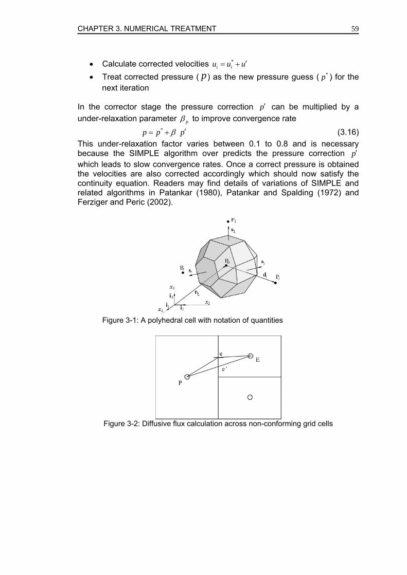
CHAPTER 3. NUMERICAL TREATMENT
59
• Calculate corrected velocities *i iu u u′= +
• Treat corrected pressure ( p ) as the new pressure guess ( *p ) for the next iteration
In the corrector stage the pressure correction p′ can be multiplied by a under-relaxation parameter pβ to improve convergence rate
*p p pβ ′= + (3.16) This under-relaxation factor varies between 0.1 to 0.8 and is necessary because the SIMPLE algorithm over predicts the pressure correction p′ which leads to slow convergence rates. Once a correct pressure is obtained the velocities are also corrected accordingly which should now satisfy the continuity equation. Readers may find details of variations of SIMPLE and related algorithms in Patankar (1980), Patankar and Spalding (1972) and Ferziger and Peric (2002).
Figure 3-1: A polyhedral cell with notation of quantities
Figure 3-2: Diffusive flux calculation across non-conforming grid cells
CHAPTER 3. NUMERICAL TREATMENT
60
BIBLIOGRAPHY Anderson, D. A., Tannehill, J. C., Pletcher, R. H. 1984. Computational Fluid mechanics and heat transfer. Hemisphere publishing corporation. ISBN 0-89116-471-5. Boris, J. P., Grinstein, F. F., Oran, E. S., Kolbe, R. L. 1992. New insights into LES. Fluid Dyn. Res. 10, 199-228. Breuer, M., Rodi, W. 1994. LES of turbulent flow through a straight square duct and 1800 bend. Voke, P. et al. (Eds), Direct and LES I. Kluwer Academic Publishers, Dordrecht. 273-285. Ferziger, J. H., Peric, M., 2002. Computational Methods for Fluid Dynamics. Springer, 3rd edition. FLUENT 6.2, User Guide. 2001. Fluent Inc., USA. Kravchenko, A. G., Moin, P. 1997. On the effects of numerical errors in large eddy simulation of turbulent flows. J. Comp. Phys. 131. 310-322. Patankar, S. V. 1980. Numerical heat transfer and fluid flow. McGraw-Hill Book Company. ISBN 0-07-048740-5. Patankar, S. V., Spalding, D. B. 1972. A calculation procedure for heat, mass and momentum transfer in three-dimensional parabolic flows. Int. J. Heat Mass Transfer 15, 1787–1806. Pope, S. B. 2000. Turbulent Flows. Cambridge university press. ISBN 0-521-59125-2.
CHAPTER 4. CHANNEL FLOW
61
Chapter 4 . CHANNEL FLOW
4.1). INTRODUCTION The geometric simplicity and availability of large amounts of data has made the simple channel flow widely popular amongst researchers. The channel flow bounded by two solid walls (assumed to be infinitely long and wide surfaces), serves as the validation case for any new turbulence model or code development. Hence, before launching a complex flow simulation testing a fully developed channel flow is an obvious choice. In the current study which is focused on simulation of flow around cylinder bodies, the idea of testing fully developed channel flow is also valid. This enables one to test the suitability of the prototype version of the commercial code that is being used; the validity of the new user programming subroutines, effects of various grid topologies on flow statistics and an application of new subgrid-scale models.
4.2). LITERATURE REVIEW For a fully developed channel flow a wide variety of experimental and numerical studies exist. In the numerical context both Direct Numerical Simulation (DNS) and Large Eddy Simulation (LES) data are available from a number of published sources. In the current chapter only DNS data will be used for comparisons. The experimental data of Eckelmann (1970) and Hussain & Reynolds (1975) are also available but will not be utilized. Eckelmann (1970) performed an experimental study for a fully developed channel flow at a fairly low Reynolds number ( ReC ) of 2,800 to 4,100 based on the centreline velocity and half width of the channel flow. Hussain & Reynolds (1975) on the other hand conducted the experimental study using hot wire anemometry at a higher Reynolds number of 13,800 to 32,000 utilizing similar techniques and concentrating on near wall behaviour. With improvements in computational power DNS became a reality. Perhaps the first DNS of a fully developed channel flow was performed by Kim et al. (1987). The Reynolds number based on centreline velocity ( ReC ) was 3,300 and the mesh size was 192 x 129 x 160 in streamwise, wall normal and homogeneous spanwise directions respectively. Higher order statistics such
CHAPTER 4. CHANNEL FLOW
62
as flatness and skewness were also taken into consideration and special attention was paid to the near wall behaviour. Moser et al. (1999) performed DNS for the channel flow at three different Reynolds numbers ( Reτ = 180, 395 and 590) all based on wall friction velocity and half width of the channel. A total of 2.1, 9.4 and 37.8 million cells were used for the simulation of the aforementioned three cases respectively. In addition to the flatness and skewness, production and dissipation were also reported in the log region of the wall. Apart from DNS, extensive LES data is also available. Deardorff (1970) performed the first large eddy simulation for a channel flow at a high Reynolds number with a uniform grid distribution and a mesh size of only 5,760 cells which hardly qualifies as an LES due to the coarse gird resolutions used. Perhaps the first true LES was performed by Moin and Kim (1982) with a mesh of 0.51 million cells (64 x 63 x 128). The Reynolds number based on the bulk velocity was 13,800 and the Smagorinsky constant was locally damped via the Van-Driest wall damping function. Piomelli et al. (1988) performed a test of combinations of filters and SGS models for large eddy simulation at a low Reynolds number with three different girds; coarse (16 x 63 x 16), medium (32 x 63 x 32) and fine (64 x 63 x 64). It was concluded by the authors that a strong relationship exists between the subgrid-scale model and the type of the filter used. Piomelli (1993) performed LES for higher Reynolds numbers of Reτ = 1,050 and 2,000. Fourier-Chebyshev pseudo-spectral collocation schemes were used and with two different grids for the low Reynolds number much like DNS study. The results were quite promising in terms of lower order statistics, velocities and Reynolds stresses. However, higher order statistics such as flatness and skewness had a poor agreement with DNS and experimental data. It was concluded that some sort of modification was required in the Smagorinsky model to account for the transfer of energy from smaller scales back to the larger scales; a fact which later became known as backscatter. At a moderate Reynolds number of Reτ = 180, Cziesla et al. (1999) investigated fully developed channel flow with periodic boundary conditions3. Majander and Siikonen (2002) performed fully developed channel flow simulations at Reynolds number of Reb = 2,800 and 12,500 based on the bulk velocity and half width of the channel. Three different grids were tested with and without SGS modelling for the low Reynolds number; coarse (16 x 64 x 16), medium (32 x 64 x 32) and fine (64 x 64 x 64). For the Smagorinsky model, the model coefficient was damped with the Van-Driest wall damping function. For the higher Reynolds number only a single mesh was tested with a total of 65,536 cells (32 × 64 × 32). For the low Reynolds number case the coarse mesh was unable to predict the near-wall region correctly. However, the simulation with the finer grid and no SGS modelling produced quite 3 Commonly known as the cyclic boundary condition. The outflow from one domain is mapped as the inflow of another thus making that direction infinite. However, the two domains should have matching grids otherwise some sort of spatial interpolation is required.
CHAPTER 4. CHANNEL FLOW
63
promising results. It was seen that the resolved Reynolds stresses were damped (or excessively damped?) by the eddy viscosity when the SGS modelling was turned on. Volker et al. (2002) performed an LES at a Reynolds number ( Reτ ) of 590 using a grid of 32 x 257 x 32. The idea behind their study was to find an optimal LES model based on the DNS data of Moser et al. (1999). Such an optimal model would then be later tested at high Reynolds numbers for wall bounded flows. However, their effort proved to be futile as the authors accepted that their model was clearly not ready for LES applications. To test the vortex method of Sergent (2002) recently Mathey et al. (2006) performed a channel flow simulation at a Reynolds number ( Reτ ) of 395. It was concluded that the technique of Sergent (2002) was clearly superior to the usual random turbulence generation methodology as the results converged much faster and were found to be in close agreement of DNS data of Moser et al. (1999).
4.3). CASE DESCRIPTION As already explained the idea behind testing fully developed channel flow is to test the suitability of the code. Yet another reason is to test the user subroutines and the new subgrid-scale models implemented in the current code. A grid dependence study was also included on the channel flow cases to test non-conforming meshes. However, due to complexity and the number of cases tested the non-conforming mesh cases and their effects on flow parameters will not be reported in this section. The readers can find details of these tests in Appendix B. In the current report emphasis will be on first and second order statistics and general flow physics. Higher order statistics such as flatness and skewness will not be discussed in the context of this thesis. Hence, the tests of channel flow with various models and geometries presented here are not claimed to be complete. However, they give some measure of the accuracy of the commercial codes used in an LES mode. The channel flow geometry consists of two solid walls only, top and bottom as shown in Figure 4-1. The flow is assumed to be homogeneous in the other two directions which are the streamwise and spanwise directions. The dimensions of this channel flow may vary from case to case. Moser et al. (1999) uses a channel flow of dimensions 2 2πδ δ πδ× × for Reynolds numbers ( Reτ ) of 395 and 590, Piomelli et al. (1993) uses the dimensions of 4 2πδ δ πδ× × , Hughes et al. (2001) uses the dimensions of 2 2 4 / 3πδ δ πδ× × . In the current test cases we keep the dimensions as 2 2πδ δ πδ× × where δ =1 and the flow Reynolds number based on wall friction velocity ( Reτ ) is 395. The DNS data of Moser el al. (1999) that will be used for comparisons is also for the same geometry size. Figure 4-1 shows the channel flow geometry where X-axis shows the streamwise direction, Y-axis the wall normal direction and Z-axis the spanwise direction.
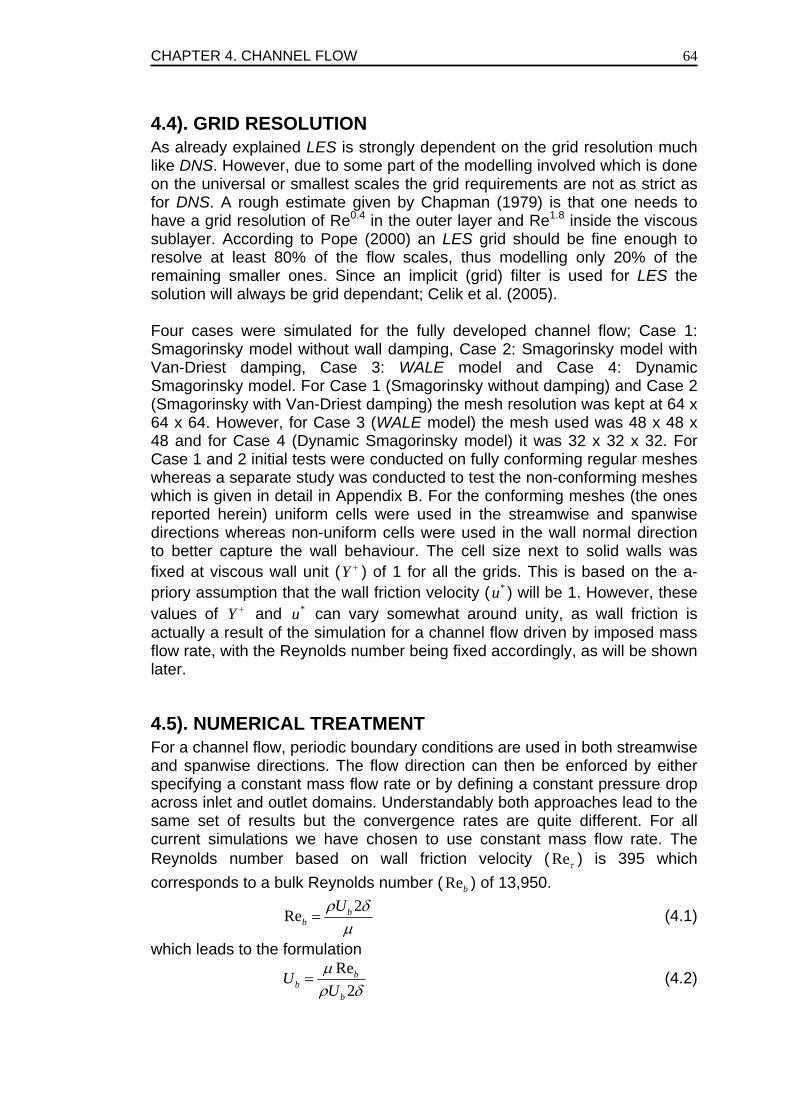
CHAPTER 4. CHANNEL FLOW
64
4.4). GRID RESOLUTION As already explained LES is strongly dependent on the grid resolution much like DNS. However, due to some part of the modelling involved which is done on the universal or smallest scales the grid requirements are not as strict as for DNS. A rough estimate given by Chapman (1979) is that one needs to have a grid resolution of Re0.4 in the outer layer and Re1.8 inside the viscous sublayer. According to Pope (2000) an LES grid should be fine enough to resolve at least 80% of the flow scales, thus modelling only 20% of the remaining smaller ones. Since an implicit (grid) filter is used for LES the solution will always be grid dependant; Celik et al. (2005). Four cases were simulated for the fully developed channel flow; Case 1: Smagorinsky model without wall damping, Case 2: Smagorinsky model with Van-Driest damping, Case 3: WALE model and Case 4: Dynamic Smagorinsky model. For Case 1 (Smagorinsky without damping) and Case 2 (Smagorinsky with Van-Driest damping) the mesh resolution was kept at 64 x 64 x 64. However, for Case 3 (WALE model) the mesh used was 48 x 48 x 48 and for Case 4 (Dynamic Smagorinsky model) it was 32 x 32 x 32. For Case 1 and 2 initial tests were conducted on fully conforming regular meshes whereas a separate study was conducted to test the non-conforming meshes which is given in detail in Appendix B. For the conforming meshes (the ones reported herein) uniform cells were used in the streamwise and spanwise directions whereas non-uniform cells were used in the wall normal direction to better capture the wall behaviour. The cell size next to solid walls was fixed at viscous wall unit (Y + ) of 1 for all the grids. This is based on the a-priory assumption that the wall friction velocity ( *u ) will be 1. However, these values of Y + and *u can vary somewhat around unity, as wall friction is actually a result of the simulation for a channel flow driven by imposed mass flow rate, with the Reynolds number being fixed accordingly, as will be shown later.
4.5). NUMERICAL TREATMENT For a channel flow, periodic boundary conditions are used in both streamwise and spanwise directions. The flow direction can then be enforced by either specifying a constant mass flow rate or by defining a constant pressure drop across inlet and outlet domains. Understandably both approaches lead to the same set of results but the convergence rates are quite different. For all current simulations we have chosen to use constant mass flow rate. The Reynolds number based on wall friction velocity ( Reτ ) is 395 which corresponds to a bulk Reynolds number ( Reb ) of 13,950.
2Re bb
Uρ δµ
= (4.1)
which leads to the formulation
Re2
bb
b
UUµρ δ
= (4.2)
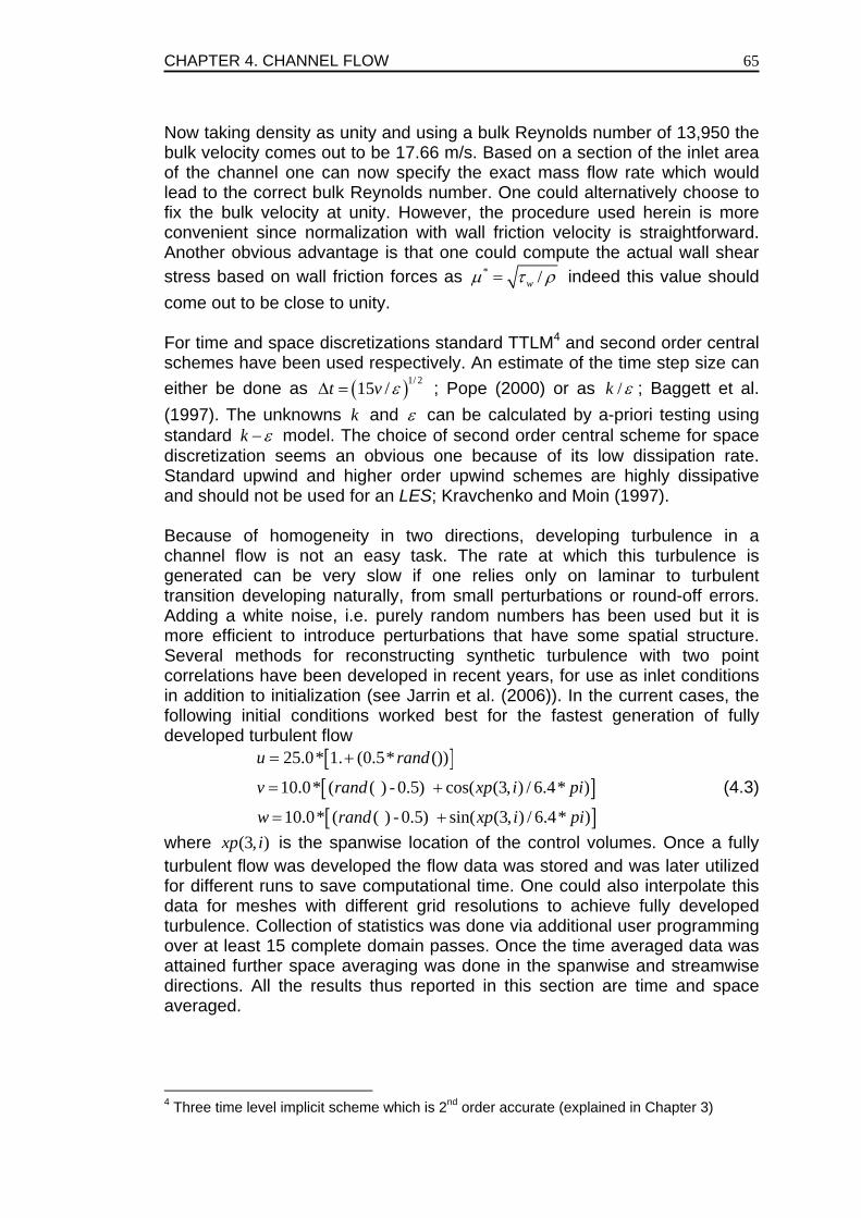
CHAPTER 4. CHANNEL FLOW
65
Now taking density as unity and using a bulk Reynolds number of 13,950 the bulk velocity comes out to be 17.66 m/s. Based on a section of the inlet area of the channel one can now specify the exact mass flow rate which would lead to the correct bulk Reynolds number. One could alternatively choose to fix the bulk velocity at unity. However, the procedure used herein is more convenient since normalization with wall friction velocity is straightforward. Another obvious advantage is that one could compute the actual wall shear stress based on wall friction forces as * /wµ τ ρ= indeed this value should come out to be close to unity. For time and space discretizations standard TTLM4 and second order central schemes have been used respectively. An estimate of the time step size can either be done as ( )1/ 215 /t v ε∆ = ; Pope (2000) or as /k ε ; Baggett et al. (1997). The unknowns k and ε can be calculated by a-priori testing using standard k ε− model. The choice of second order central scheme for space discretization seems an obvious one because of its low dissipation rate. Standard upwind and higher order upwind schemes are highly dissipative and should not be used for an LES; Kravchenko and Moin (1997). Because of homogeneity in two directions, developing turbulence in a channel flow is not an easy task. The rate at which this turbulence is generated can be very slow if one relies only on laminar to turbulent transition developing naturally, from small perturbations or round-off errors. Adding a white noise, i.e. purely random numbers has been used but it is more efficient to introduce perturbations that have some spatial structure. Several methods for reconstructing synthetic turbulence with two point correlations have been developed in recent years, for use as inlet conditions in addition to initialization (see Jarrin et al. (2006)). In the current cases, the following initial conditions worked best for the fastest generation of fully developed turbulent flow
[ ][ ][ ]
25.0* 1. (0.5* ())
10.0* ( ( ) - 0.5) cos( (3, ) / 6.4* )
10.0* ( ( ) - 0.5) sin( (3, ) / 6.4* )
u rand
v rand xp i pi
w rand xp i pi
= +
= +
= +
(4.3)
where (3, )xp i is the spanwise location of the control volumes. Once a fully turbulent flow was developed the flow data was stored and was later utilized for different runs to save computational time. One could also interpolate this data for meshes with different grid resolutions to achieve fully developed turbulence. Collection of statistics was done via additional user programming over at least 15 complete domain passes. Once the time averaged data was attained further space averaging was done in the spanwise and streamwise directions. All the results thus reported in this section are time and space averaged.
4 Three time level implicit scheme which is 2nd order accurate (explained in Chapter 3)
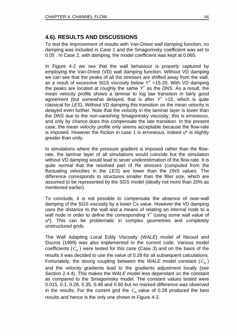
CHAPTER 4. CHANNEL FLOW
66
4.6). RESULTS AND DISCUSSIONS To test the improvement of results with Van-Driest wall damping function, no damping was included in Case 1 and the Smagorinsky coefficient was set to 0.05 . In Case 2, with damping, the model coefficient was kept at 0.065. In Figure 4-2 we see that the wall behaviour is properly captured by employing the Van-Driest (VD) wall damping function. Without VD damping we can see that the peaks of all the stresses are shifted away from the wall, as a result of excessive SGS viscosity below Y+ =15-20. With VD damping the peaks are located at roughly the same Y+ as the DNS. As a result, the mean velocity profile shows a laminar to log law transition in fairly good agreement (but somewhat delayed, that is after Y+ =15, which is quite classical for LES). Without VD damping this transition on the mean velocity is delayed even further. Note that the velocity in the laminar layer is lower than the DNS due to the non-vanishing Smagorinsky viscosity, this is erroneous, and only by chance does this compensate the late transition. In the present case, the mean velocity profile only seems acceptable because the flow-rate is imposed. However the friction in case 1 is erroneous, indeed u* is slightly greater than unity. In simulations where the pressure gradient is imposed rather than the flow-rate, the laminar layer of all simulations would coincide but the simulation without VD damping would lead to sever underestimation of the flow-rate. It is quite normal that the resolved part of Re stresses (computed from the fluctuating velocities in the LES) are lower than the DNS values. The difference corresponds to structures smaller than the filter size, which are assumed to be represented by the SGS model (ideally not more than 20% as mentioned earlier). To conclude, it is not possible to compensate the absence of near-wall damping of the SGS viscosity by a lower Cs value. However the VD damping uses the distance to the wall and a means of relating an internal node to a wall node in order to define the corresponding Y+ (using some wall value of u*). This can be problematic in complex geometries and completely unstructured grids. The Wall Adapting Local Eddy Viscosity (WALE) model of Nicoud and Ducros (1999) was also implemented in the current code. Various model coefficients ( WC ) were tested for this case (Case 3) and on the basis of the results it was decided to use the value of 0.28 for all subsequent calculations. Fortunately, the strong coupling between the WALE model constant ( WC ) and the velocity gradients lead to the gradients adjustment locally (see Section 2.4.4). This makes the WALE model less dependant on the constant as compared to the Smagorinsky model. The constant values tested were 0.015, 0.1, 0.28, 0.35, 0.48 and 0.60 but no marked difference was observed in the results. For the current grid the WC value of 0.28 produced the best results and hence is the only one shown in Figure 4-3.
CHAPTER 4. CHANNEL FLOW
67
Nicoud and Ducros (1999) highlighted the problems with the Smagorinsky model, in particular the non-physical behaviour of the SGS viscosity near solid walls, which requires ad-hoc damping. The WALE model proposes using the traceless symmetric part of the square of the velocity gradient tensor instead of just using the strain rate tensor. The WALE operator ( d d
ij ijδ δ ) from equation (2.51) now behaves like Y2. Thus, a scaling is now required to achieve the true wall behaviour of Y3. This scaling is done on purely physical reasoning and hence requires further justification. On the other hand since the WALE model is based on true velocity gradient tensor it is more robust than the Smagorinsky model. The WALE model can detect turbulent structures with large strain rates, rotation rates or both which is a great advantage over Smagorinsky model which is unable to reproduce the laminar to turbulent transition because of large invariant of ij ijS S in case of pure shear. The implementation of Dynamic Smagorinsky model (see Appendix D) in the current code has been somewhat problematic. Unfortunately the explicit filtering which is mandatory in the dynamic cases is not very straightforward in a general unstructured code. Various test filters were used for the explicit filtering which included, simple averaging, inverse distance averaging and weighted distance averaging over the neighbours. The filter width was kept as a variable for all the cases and it was ensured that the filter area contains both the cell neighbours and the neighbours of neighbours. Thus for a Cartesian grid the explicit filter for every cell contained at most 27 cells. Admittedly near the walls and on corners this number would substantially decrease. The unavailability of the source code meant that the filter cells for every cell in the domain had to be sorted out before hand. The added computations involved in the programming of the model and the averaging of all variables for every cell leads to a huge increase in computational cost. Thus for the dynamic model the grid resolution had to be reduced to 32 x 32 x 32. Nevertheless, the results which are shown in Figure 4-4 seem to be very promising. The agreement of the mean velocity profile in the log–layer is particularly remarkable. On the other had there is again a slight underestimation of the velocity in the viscous sublayer, which may be due to the fairly coarse grid, since the Dynamic model is usually considered quite efficient in predicting laminar-turbulent transition. A complete comparison between all the models (Smagorinsky, WALE and dynamic Smagorinsky) is given in Figure 4-5. We see from Figure 4-5(a) that the wall behaviour is best captured by the WALE model. The worse case is for Smagorinsky without wall damping. The grid used for the dynamic model is the coarsest, yet this model is still far better than Smagorinsky without wall damping. For the mean streamwise stress comparison which is shown in Figure 4-5(b) the dynamic model clearly allows higher levels of fluctuations than all other models. Away from the wall the profile seems to be collapsing to the DNS
CHAPTER 4. CHANNEL FLOW
68
data of Kim et al. (1987). This, however, could be a coincidence for this specific grid. Indeed many of channel flow LES on finer grids show an overestimation of the streamwise fluctuations, yet an underestimation of the wall normal component. Indeed the peak value of streamwise fluctuation is also overestimated here, while the mean normal stress and mean spanwise stress distributions are lower, but still the Dynamic model seems to be superior to all other models, the only drawback being the mean velocity in the viscous sublayer (as well as the costly computation time). The model seems to be highly sensitive to the explicit filtering especially in regions very close to the wall. It is thus anticipated that with a finer mesh the wall behaviour will be better captured. However, the non-uniformity in the gird distribution in the wall normal direction will always be an important factor in determining the accuracy of the dynamic model where the cell distribution in one direction is always smaller than the distribution in the other direction. The dynamic model constant ( dynC ) is not averaged in time or space. However, to avoid instabilities in the flow the constant has to be clipped for higher negative values. Clipping the constant in the negative values is not desired but one has to ensure that the solution will remain stable in time. In the current case the constant is allowed to vary between -0.01 and 0.23. This allows for a small amount of backscatter which is desirable and is one of the key factors in the selection of any LES model. In commercial codes such as Fluent 6.2, the backscatter is not allowed at all, the constant is clipped for values lower than zero. This ensures stability of the code on one hand but questions the accuracy or even the advantage of the use of the dynamic procedure on the other.
4.7). CONCLUSIONS Fully developed channel flow was simulated via LES with different models; Smagorinsky without wall damping, Smagorinsky with Van-Driest wall damping, WALE and dynamic Smagorinsky model. Due to computational costs attached to the models the same grid resolution could not be utilized for all the cases. The grid used for the WALE and the dynamic model was thus substantially coarser than the ones used for Smagorinsky model. However, the WALE model and the dynamic model still seemed to perform quite well, and we recall that they have the advantage of not requiring a Y+ dependent damping function which is complicated with unstructured grids. The filtering approach used in the implementation of the dynamic model and the stability problems inherently attached to the model are still under investigation. These complications and most of all the added computational cost of the model, which is approximately 10 times higher than the Smagorinsky model, led us to abandon the idea of testing it in the industrial applications investigated in following chapters. The WALE model on the other hand is easy to implement, does not require external local wall damping functions and is computationally less expensive than the dynamic model. However, the Smagorinsky model with Van-Driest
CHAPTER 4. CHANNEL FLOW
69
wall damping function is still a promising choice for the future calculations. This is mainly due to its computational cost which is almost 3 times less than the WALE model and 10 times less than the dynamic model. It is very likely that part of the extra cost is down to the non-optimal coding via user defined functions, but still the Dynamic model is bound to be expensive in an unstructured code.
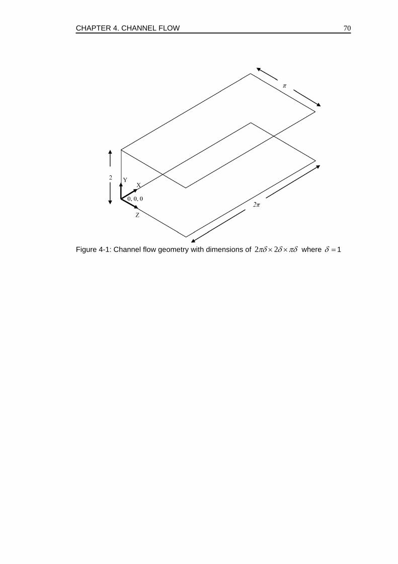
CHAPTER 4. CHANNEL FLOW
70
Figure 4-1: Channel flow geometry with dimensions of 2 2πδ δ πδ× × where δ = 1
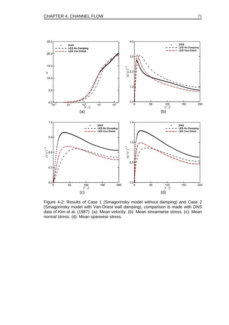
CHAPTER 4. CHANNEL FLOW
71
(a) (b)
(c) (d)
Figure 4-2: Results of Case 1 (Smagorinsky model without damping) and Case 2 (Smagorinsky model with Van-Driest wall damping), comparison is made with DNS data of Kim et al. (1987). (a): Mean velocity. (b): Mean streamwise stress. (c): Mean normal stress. (d): Mean spanwise stress.
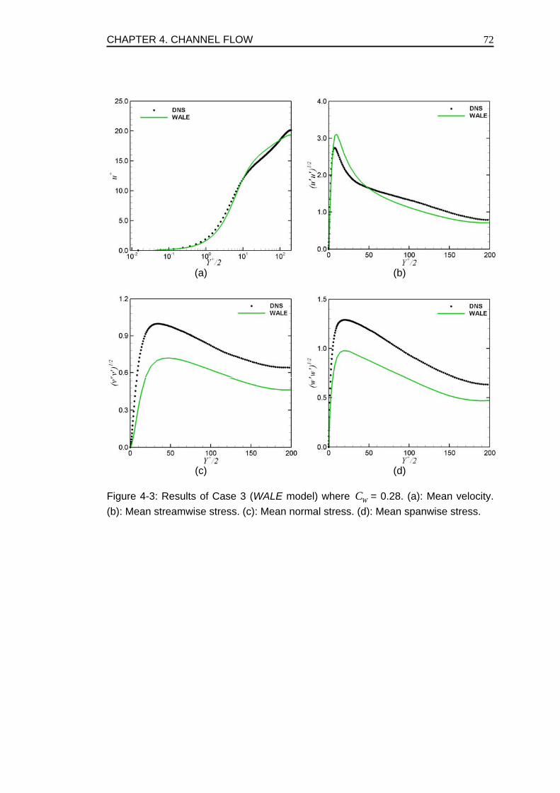
CHAPTER 4. CHANNEL FLOW
72
(a) (b)
(c) (d)
Figure 4-3: Results of Case 3 (WALE model) where WC = 0.28. (a): Mean velocity. (b): Mean streamwise stress. (c): Mean normal stress. (d): Mean spanwise stress.
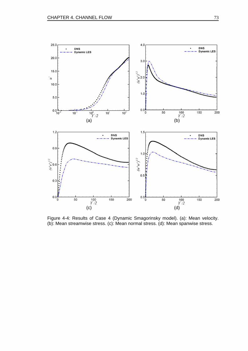
CHAPTER 4. CHANNEL FLOW
73
(a) (b)
(c) (d)
Figure 4-4: Results of Case 4 (Dynamic Smagorinsky model). (a): Mean velocity. (b): Mean streamwise stress. (c): Mean normal stress. (d): Mean spanwise stress.
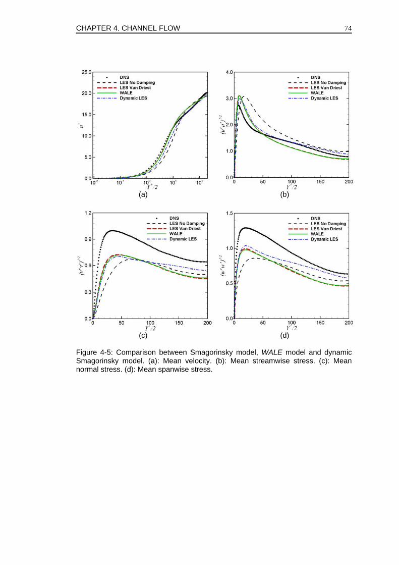
CHAPTER 4. CHANNEL FLOW
74
(a) (b)
(c) (d)
Figure 4-5: Comparison between Smagorinsky model, WALE model and dynamic Smagorinsky model. (a): Mean velocity. (b): Mean streamwise stress. (c): Mean normal stress. (d): Mean spanwise stress.
CHAPTER 4. CHANNEL FLOW
75
BIBLEOGRAPHY Celik, I. B., Cehreli, Z. N., Yavuz, I. 2005. Index of resolution quality for Large Eddy Simulations. J. Fluids Eng. 127, 949-958. Chapman, D. R. 1979 Computational aerodynamics development and outlook. AIAA J. 17, 1293. Cziesla, T., Biswas, G., Mitra, N. K. 1999. Large Eddy Simulation in a Turbulent Channel Flow Using Exit Boundary Conditions. Int. J. Num. Meth. Fluids. 30, 763. Deardoff, J. W. 1970. A numerical study of three-dimensional turbulent channel flow at large Reynolds numbers. J. Fluid Mech. 41, 453. Kravchenko, A. G., Moin, P., 1997. On the effect of numerical errors in large eddy simulation of turbulent flows. J. Comp. Phys. 131, 310-322. Eckelmann, H. 1974. The structure of the viscous sublayer and the adjacent wall region in a turbulent channel flow. J. Fluid Mech. 41, 453. Hussain, A. K. M. F., Reynolds, W. C. 1975. Measurements in fully developed turbulent channel flow. Trans. ASME. J. Fluids Eng. 97, 568. Jarrin, N., Benhamadouche, S., Laurence, D., Prosser, R. 2006. A synthetic eddy method for generating inflow conditions for Large Eddy Simulations. Int. J. Heat Fluid Flow. Vol 27(4), 585-593. Kim, J., Moin, P., Moser, R. D. 1987. Turbulence statistics in fully developed channel flow at low Reynolds number. J. Fluid Mech. 177, 133. Mathey, F., Cokljat, D., Bertoglio, J. P., Sergent, E. 2006. Assessment of the vortex method for Large Eddy Simulation inlet conditions. Progress in Computational Fluid Dynamics, An International Journal (PCFD), Vol. 6, No. 1/2/3, 2006. Moin, P., Kim, J. 1982 Numerical investigation of turbulent channel flow. J. Fluid Mech. 118, 341. Moser, R. D., Kim, J. Mansour, N. N. 1999. Direct numerical simulation of turbulent channel flow up to Re=590. Phys. Fluids. 11, 943. Nicoud, F., Ducros, F. 1999. Subgrid scale stress modelling based on the square of the velocity gradient tensor. Flow, Turb. Comb. Vol 62, 183-200.
CHAPTER 4. CHANNEL FLOW
76
Piomelli, U., Moin, P., Ferziger, J. H. 1988. Model consistency in large eddy simulation of turbulent channel flow. Phys. Fluids. 31, 1884. Piomelli, U., 1993. High Reynolds number calculation using the dynamic Subgrid-scale stress model. Phys. Fluids. 6, 1484. Pope, S. B., 2000. Turbulent Flows. Cambridge university press, 1st edition. Sergent, E. 2002. PhD Thesis. L’Ecole Centrale de Lyon. Volker, S., Moser, R. D., Venugopal, P. 2002. Optimal large eddy simulation of turbulent based on direct numerical simulation statistical data. Phys. Fluids. 14, 3675.
CHAPTER 5. FINITE CANTILEVER CYLINDERS
77
Chapter 5 .
REVIEW OF FLOW AROUND FINITE CYLINDERS
5.1). INTRODUCTION The cantilevered cylinder (sometimes referred to as a finite cylinder) with one end fixed and the other free to vibrate has been used extensively to study the dynamics of flows around cylinder bodies. The flow over a finite cylinder free end has a complicated three dimensional wake structure where the free end plays a direct and significant factor in flow three-dimensionality. The three- dimensionality of the flow around the finite cylinder is much more pronounced than for cylinders with both ends fixed. This is due to the counter-rotating vortices generated by the free end itself. Gerrard (1978) shows that the flow behind a cantilever cylinder becomes fully turbulent in the Reynolds number range of 260-300. Unal and Rockwell (1988) also suggest the same range. However, the common understanding is that turbulence starts near the lower value of this range. Various test cases will be looked upon with different aspect (height to diameter) ratios via published experimental work and current numerical simulations. Some of the investigations will tackle issues relating to vortex shedding, 3-D fluctuations in the wake, lift and drag (instantaneous and RMS) and pressure distributions. In the next few sections we shall discuss the various studies already carried out and well documented in literature in relation to such configurations.
5.2). LITERATURE REVIEW FOR FINITE CYLINDERS
5.2.1). VORTEX SHEDDING BEHIND CYLINDERS One of the most extensive experimental studies for finite cylinders is the one done by Park and Lee (2000), (2002) and (2004). The first paper in this series tests various aspect ratio cylinders at a Reynolds number of 20,000 based on cylinder diameter. This was done to study the effect of cantilever cylinder aspect ratio on vortex shedding, cylinder vibrations and three dimensionality of the flow. Park and Lee (2000) show that as the aspect ratio decreases the vortex shedding frequency also decreases. This has also been
CHAPTER 5. FINITE CANTILEVER CYLINDERS
78
shown by Farivar (1981), who found out that the vortex shedding frequency disappeared for aspect ratios smaller that 7.5. But on the other hand Zdravkovich et al. (1989) reported irregular and intermittent vortex shedding for cylinders with aspect ratios of 2. However, due to complexity of the flow such direct conclusions cannot be drawn especially since the vortex shedding itself depends upon a number of parameters. Seto et al. (1992) studied the effect of some of these parameters on the vortex shedding frequency. The vortex shedding and its governing parameters will thus be investigated and discussed in detail in the next chapter. Park and Lee (2002) show a study on the flow characteristics for a finite cylinder in various atmospheric boundary layers where the comparisons are done with the uniform flow over finite cylinders. In Park and Lee (2004) the study is further prolonged to test the effects of end shape. Only one aspect ratio of 6 is looked upon with flat (same as round cylinder), beveled (slant at corners), radiussed (tapered ends) and hemispherical end shapes. The study of coherent eddies is also a very interesting area for the cylinder flows. Coherent structures are specified eddies which are reproducible under definite conditions. Shirakashi (1988) classifies these coherent structures into three categories. The first category is the one in which the eddy formation process and configuration is similar to an eddy formed at much lower Reynolds number under similar boundary conditions. Karman Vortices are a classical example of such structures. At very high Reynolds number where turbulent eddies mimic the effect of molecular viscosity, the Karman vortices collapse and vortex streets are reorganized. These are type two vortices. Flow past a building or around an isolated mountain shows signs of presence of such vortices as is also stated by Kimura (1982). Finally the rearrangement of vorticity in the non-uniform mean velocity distribution results in coherent structure formation; type three vortices. The classical example is the banana vortices in a turbulent boundary layer observed by Fukunishi and Sato (1983). Shirakashi et al. (1988) show a study of these coherent structures behind a circular cylinder at Re = 850 and 1,700 experimentally by smoke wire measurement. This paper shows the breaking up of Karman vortices into smaller ones and then reorganization and bending of these smaller vortices to form horseshoe or arch like vortices behind the cylinder. Further downstream these vortices look like banana shaped vortices. Okubo et al. (1988) conducted a numerical study using a vortex filament model to further study these spoon or banana like vortices. This study supports the idea that these strangely deformed vortices are in fact a result of breaking and distortion of Karman vortices. A third paper in the same series by Yamane et al. (1988) is a further experimental study of these vortices for a much higher Reynolds number range. Shirakashi et al. (1988) reported that the size of the spoon shaped vortex street is around eight times the diameter of the cylinder. Yamane et al. (1988) also states that the largest scale vortex in the coherent structure has a very strong effect on the Reynolds stress and also in the production of the turbulence kinetic energy. In fact Alfonsi and Giorgini (2002)
CHAPTER 5. FINITE CANTILEVER CYLINDERS
79
study the time dependent impulsively started cylinder behavior and draw the same conclusion. They record that the coherent structures behind the cylinder are the most energetic modes of the entire flow. It even suggests that the flow field could be described in terms of a few modes containing the most energetic modes of the flow. Roshko (1953) and Schlichting (1979) proved that the Strouhal number depends weakly on the Reynolds number. The Strouhal number is defined as
DSt fU
= (3.17)
where f is the vortex shedding frequency, D the diameter of the cylinder and U the velocity (either free stream or bulk velocity). Lei et al. (1999) has done an extensive study showing that the Strouhal number must be calculated on the basis of free stream velocity and not on the local or gap velocity in cases which involve tube bundles. However correlations do exist on the basis of gap velocity while calculating the Strouhal number. For the current simulations comparisons will be based on both free stream and gap velocity and will be clearly marked by 0U or gapU respectively.
5.2.2). LIFT AND DRAG FORCES The unsteady pressure fluctuations on any cylinder lead to highly fluctuating lift and drag forces where these forces are strongly dependent upon the aspect ratio of the cylinder. Wieselsberger (1922) showed that the drag force on a cylinder decreases as the aspect ratio becomes smaller. In essence most of the research for flows around cylinders revolve around lift and drag calculations with a primary interest in reduction of such parameters to avoid extensive vibrations. Broadly categorized, for bluff bodies two types of flow control techniques are generally used; active and passive techniques. In active flow control techniques the flow is altered by supplying a constant external source such as jet blowing, acoustic excitation or by some other means. Although reasonable such techniques are not preferred in a longer run due to the cost attached to them. The passive flow techniques on the other hand are highly popular and widely employed. In such techniques the flow is altered for a much desired drag reduction by modifying the original shape of the geometry or by insertion of an additional control body (generally a small cylinder or a rod). A prime example is Lee et al. (2004) in which a small control rod has been used to minimize the total drag force on the cylinder. It has also been shown that the insertion point of this control rod is far more important than any other parameter. The insertion regions based effectively on drag response are classified as cavity mode (where the gap space between the cylinder and the control rod is 1.5) and impingement mode (where the gap space is 2.17). Another prime example of passive flow control technique is that of Kawamura et al. (1984b) in which the drag reduction is achieved via playing with the surface roughness of the cylinder which effectively alters the flow by lowering the critical Reynolds number.
CHAPTER 5. FINITE CANTILEVER CYLINDERS
80
A slightly different scenario is investigated by Lei et al. (1999), in which the cylinders lift and drag properties are studied in the presence of a solid wall. A strong correlation is found between the gap distance (between the wall and cylinder) and the vortex shedding frequency which in turn affects the lift and drag parameters. For narrow gap distances the vortex shedding is suppressed causing lower values of lift and drag whereas for higher gap ratios the scenario is quite the opposite. Issues such as dependence of lift and drag parameters on free stream velocity should also be addressed. According to Norberg (2003) the root mean square (r.m.s) drag is more sensitive to the increase in free stream velocity than the r.m.s lift coefficient. The study shows that with a five fold increase in inlet velocity the drag coefficient is increased by 600 times whereas the lift coefficient is increased by only 15 percent.
5.2.3). PRESSURE FLUCTUATIONS AND CYLINDER VIBRATIONS In finite cylinders the mean pressure on the windward side decreases as one moves towards the free end due to a reduction in blockage effects. Thus, one could conclude that the mean pressure on the cylinder surface is a direct result of the free end interference; Park and Lee (2000). The surface pressure distribution for any cylinder body oscillates at the vortex shedding period. These pressure variations are consistent with periodic changes of circulation around the cylinder body. For correlations and the discussion to follow, the coefficient of pressure is defined as
( )
20
2 refP
p pC
Uρ−
= (3.18)
where p is the surface pressure, refp the reference pressure and 20 / 2Uρ the
dynamic pressure. Vortex induced vibrations of a circular cylinder are a fundamental problem in flow induced vibrations. Numerous nuclear power plant shutdowns are due to this simple yet complex phenomenon. The damage caused in the Japanese Nuclear Development institute, Monju in 19955 was due to streamwise flow induced vibrations. Thus numerous efforts have been revolving around this phenomenon for the last decade. Worth mentioning series of study in this area is of Okajima et al. (2001), Okajima et al. (2002), Nakamura et al. (2001a) and Nakamura et al. (2001b). In Okajima et al. (2001) flow induced in-line oscillation of a circular cylinder of aspect ratio of 10 is experimentally studied and is compared to the oscillations for a 2-D or infinite cylinder. Nakamura et al. (2001a) state that cylinder aspect ratio plays a vital role in the vibrations study. It is observed that cylinders with aspect ratios smaller than 10 show only one excitation region. On the other hand for higher aspect ratios of 14 and above multiple excitation regions are recorded. Nakamura et al. (2001b) numerically investigate the flow around a finite cylinder of aspect
5 Okajima et al. (2001)
CHAPTER 5. FINITE CANTILEVER CYLINDERS
81
ratio 5. This study provides a good comparison between the authors previous experimental findings and current numerical simulations. When understanding the cylinder vibrations one must keep in mind that the vortex streets formed in cross flow over tubes or cylinders arise only if the Reynolds number reaches a certain critical value. According to Wang et al. (2003) the vortex shedding produces a periodic excitation which effectively leads to intense cylinder vibrations. The study uses experimental data for a freely vibrating cylinder to form a new model. This new model is then implemented to study the vortex induced vibrations of an elastic cylinder (a phenomenon beyond the scope of present study). So far we have only discussed vibrations of cylinders due to vortex shedding. Indeed this is one of the main factors, but there is yet another aspect of flow that should not be neglected when looking at the cylinder flows. Kitagawa et al. (1999) study the vibrations in cylinders due to free stream velocity. The free stream induced vibrations occur only when the inlet or free stream velocity becomes greater than a threshold value. These free stream vibrations commonly known as end cell induced vibrations (ECIV) are directly dependent upon the tip associated vortex shedding and are thus a characteristic of flow around finite cantilever cylinders. It is shown that although the vortex induced vibrations (VIV) are nearly steady, the ECIV's are rather unsteady, having high amplitudes of oscillation. It is concluded that at wind speeds where the frequency of tip associated vortices coincides with the natural frequency of the body the ECIVs start. This phenomenon was also observed by Kitagawa et al. (1998), in an earlier study from the same author.
5.2.4). NUMERICAL SIMULATION OF FLOWS AROUND CYLINDERS USING LES As discussed previously with an increase in computational power Large Eddy Simulation (LES) has become a widely popular tool. Recent numerical work done on both finite and infinite cylinders will be discussed in detail in this section. Issues such as sources of errors, discretization schemes, subgrid-scale (SGS) modelling and comparison of results to experimental data will be looked upon. Breuer (1998) has done a very extensive study on LES of flow over a cylinder at a Reynolds number of 3,900. The paper not only discusses the flow physics but also addresses various parameters such as discretization schemes, sources of errors and SGS models. For any LES the sources of errors can be broadly categorized as; modelling errors, discretization errors and convergence errors. Modelling errors describe the difference between the behavior of physical system and the exact solution of the mathematical model. In LES this error might appear due to one or more of; modeling assumptions or approximations (SGS models), filtering, boundary conditions or by the governing equations themselves. Breuer (1998) tests the cylinder
CHAPTER 5. FINITE CANTILEVER CYLINDERS
82
configuration with three different models; Smagorinsky model, dynamic Smagorinsky model (based on Germano et al. (1991)) and no SGS model. For the Smagorinsky model the constant is set to 0.1 and local wall damping function (Van-Driest) is employed. Due to the low dissipation of the numerical schemes the Smagorinsky and the dynamic Smagorinsky model produced better results than the no SGS model approach. The discretization error is the difference between the exact solution of the mathematical model and the exact solution of the discretized equation. Breuer (1998) tested five different schemes; hybrid (combination of upwind differencing and central differencing), second order central differencing (CD-2), fourth order central differencing (CD-4), hybrid linear/parabolic and Quadratic Upwind Interpolation for Convective Kinematics (QUICK). The hybrid scheme showed no wiggles or boundedness problems but was found to be highly diffusive. The second order central difference scheme on the other hand leads to truncation error terms proportional to square of the cell spacing. Breuer (1998) reports boundedness problems with this scheme especially for coarse grids. Similar problems have previously been reported and corrective measures have been suggested by Rodi et al. (1997). According to Rodi et al. (1997) this oscillation problem can be solved by an increase in the grid resolution. With increasing Reynolds number this problem becomes more and more severe, thus the higher the Reynolds number the finer the mesh requirement. One natural solution to avoid these numerical oscillations is to keep the local or grid Peclet number ( /Pe u xρ= ∆ Γ ) below 2; see Patankar (1980). In comparison with experimental data of Ong and Wallace (1996) the best results were obtained with CD-2 and CD-4. These observations agree well with the findings of Beaudan and Moin (1994) that the upwind schemes are highly diffusive and should not be used for LES. Mittal and Moin (1997) also recommends the use of at least CD-2 scheme for an LES. For outflow boundary conditions, Breuer (1998) used a convective boundary condition. Use of such boundary conditions ensures that the vortices approach and pass the outflow boundary without significant disturbances or reflections back to the inner domain. Previously Breuer and Rodi (1996), and Breuer and Pourquie (1996) have shown that convective boundary condition works perfectly well with LES. In some cases the outflow boundary6 is also prescribed. However, since this boundary condition is highly reflective, it should be avoided where possible. Poinsot et al. (1992) elaborates that for compressible flows when a pressure distribution is convected across the outflow boundary, small pressure disturbances are reflected back into the computational domain, imposing disturbances on the approaching flow which are purely non physical. However, for incompressible cases a pressure outlet boundary condition works well for LES. The spanwise resolution is also a significant factor in any LES. Special consideration must be given to grid resolution in the spanwise or 6 far field assumption with static pressure ( statp ) of the free stream specified at the outlet
CHAPTER 5. FINITE CANTILEVER CYLINDERS
83
homogeneous direction; Kravchenko and Moin (2000) and Franke and Frank (2002). According to Kravchenko and Moin (2000) and Mittal (1996) the mean integral values are also strongly dependent upon the averaging time. Thus averaging should be done in both time and space over all homogeneous directions. Frohlich and Rodi (2004) have performed a LES of a cantilever cylinder of aspect ratio 2.5 with both Smagorinsky and dynamic Smagorinsky models. In relation to the aspect ratio of the cylinder two important correlations have been addressed; vortex shedding and lift and drag parameters. It is observed that as the aspect ratio decreases the alternating vortex shedding changes into symmetric vortices complemented by a decrease in lift and drag coefficients. Similar conclusions were drawn by experimental studies of Zdravkovich et al. (1989) and Kawamura et al. (1984a). Breuer (1998) states that it is difficult to achieve an approximate description of flow over cylinders using a Reynolds averaged Navier-Stokes equations (RANS), and that since Direct Numerical Simulations (DNS) will not become affordable in the near future, the obvious choice is LES for cylinder flows. Indeed it had been concluded earlier by Majumdar and Rodi (1985) that standard two equation turbulence models such as k ε− and k ω− are incapable of accurately predicting turbulent flows where the local anisotropy of the turbulent stress plays an important role. However, nonlinear EVM models show improved results in the calculation of dynamic loading and flow over stationary cylinders with similar configurations; Revell (2006).
5.3). CONCLUDING REMARKS In flows over cylinders the vortex shedding in the wake directly affects parameters on the cylinder itself such as pressure fluctuations, lift and drag forces where the cause of one is the effect of the other. With vortex shedding the pressure changes give rise to fluctuating lift and drag forces which lead to vibrations when the structure presents some elasticity. The aspect ratio of the cylinder also plays a key role here. When the aspect ratio of the finite cylinder is small, straight two dimensional Von Karman vortices are not produced; instead vortices are bent and distorted as they travel along the wake. The separation from the sides and the tip of the cylinder interact closely resulting in complicated vortex dynamics. A wall mounted cylinder with the one end free is a much more challenging case than a single cylinder with both ends fixed. The counter rotating vortices separated from the free end forces the flow to become three dimensional over all Reynolds number ranges. The presence of a free end not only alters the near wake but also the surface pressure distribution. Furthermore the free end makes the cylinder more prone to oscillations. For such flows there are a lot of possible parameters to be taken into consideration. However, in the current study we shall investigate the effect of aspect ratio on flow parameters such as vortex shedding, lift and drag forces and pressure profiles along the cylinder surface. LES with the classical Smagorinsky model

CHAPTER 5. FINITE CANTILEVER CYLINDERS
84
will be used and the study shall serve as an interesting starting point for later calculations of tube bundles and car mirror simulations.
CHAPTER 5. FINITE CANTILEVER CYLINDERS
85
BIBLIOGRAPHY Alfonsi, G., Giorgini, A. 2002. Temporal evolution of high order vortices in the non symmetric wake past a circular cylinder. Fluid Dyn. Res. 31. 13-39. Beaudan, P., Moin, P. 1994. Numerical experiments on the flow past a circular cylinder at a sub-critical Reynolds number. Report No. TF-62, Thermo sciences Division, Department of Mechanical Engineering, Stanford University, USA. Breuer, M. 1998. Numerical and modeling influences on large eddy simulations for the flow past a circular cylinder. Int. J. Heat Fluid Flow. 19. 512-521. Breuer, M., Pourquie, M. 1996. First experience with LES of flows past bluff bodies. In: Rodi, W., Bergeles, G., (Eds.). Proc. of the 3rd international symposium of engg. turbulence modeling and measurements, Herakilon, Crete, Greece, 27-29. Breuer, M., Rodi, W. 1996. LES of complex turbulent flows of practical interest. In: Hirschel, E. H., Flow simulation with high performance computers II. Notes on numerical fluid mechanics, Vol. 52, viewing Verlag, Braunschweig, pp. 258-274. Farivar, D. 1981. Turbulent uniform flow around cylinders of finite length. AIAA J. 19(3). 275-281. Franke, J., Frank, W. 2002. Large eddy simulation of the flow past a circular cylinder at Re=3,900. J. Wind Eng. Ind. Aero. 90. 1191-1206. Frohlich, J., Rodi, W. 2004. LES of the flow around a circular cylinder of finite height. Int. J. Heat Fluid Flow. 25. 537-548. Fukunishi, H. Sato, H. 1983. Structure of turbulent intermittent region in boundary layer. Nagare 2-3, 272. Germano, M., Piomelli, U., Moin, P., Cabot, W. H. 1991. A dynamic subgrid scale eddy viscosity model. Phys. Fluids. A. 3 (7). 1760-1765. Gerrard, J. H. 1978. The wakes of cylindrical bluff bodies at low Reynolds number. Philosophical transactions of the Royal society of London. Series A, 288. 351-382. Kawamura, T., Hiwada, M., Hibino, T., Mabuchi, I., Kamuda, M. 1984a. Flow around a finite cylinder on a flat plate. Bull. JSME 27 (232). 2142-2151.
CHAPTER 5. FINITE CANTILEVER CYLINDERS
86
Kawamura, T., Takami, H., Kuwahara, K. 1984b. Computation of high Reynolds number flow around a circular cylinder with surface roughness. AIAA J. 84-0340. Kitagawa, T., Fujino, Y., Kimura, K. 1999. Effects of free end condition on end-cell-induced vibration. J. Fluids Struct. 13. 499-518. Kitagawa, T., Wakahara, T., Funjio, Y., Kimura, K. 1998. An experimental study on vortex induced vibration of a circular cylinder tower at a high wind speed. J. Wind Eng. Ind. Aero. 69-71, 731-744. Kravchenko, A. G., Moin, P. 2000. Numerical study of flow over a circular cylinder at Re=3,900. Phys. Fluids 12 (2). 403-417. Lee, S. J., Lee, S. I., Park, C. W. 2004. Reducing the drag on a circular cylinder by upstream installation of a small control rod. Fluid Dyn. Res. 34. 233-250. Lei, C. Cheng, L., Kavanagh, K. 1999. Re-examination of the effect of a plane boundary on force and vortex shedding of a circular cylinder. J. Wind Eng. Ind. Aero. 80. 263-286. Majumdar, S., Rodi, W. 1985. Numerical calculations of flow past circular cylinder, Proceedings of 3rd symposium on Numerical and physical aspects of Aerodynamic flows, long beach CA, USA. Mittal, R. 1996. Progress on LES of flow past a circular cylinder, CTR Annual Research Briefs, Center for turbulence research, Stanford, CA 94305. 233-241. Mittal, R., Moin, P. 1997. Suitability of upwind-based finite difference schemes for large eddy simulation of turbulent flow, AIAA J. 35 (8). 1415-1417. Nakamura, A., Okajima, A. 2001a. A numerical simulation and vortex structures of in-line oscillation of an elastically supported circular cylinder. Flow induced vibrations PVP Vol 420-1, ASME. Nakamura, A., Okajima, A., Kosugi, T. 2001b. Experiments on flow induced in-line oscillation of a circular cylinder in a water tunnel, 2nd report. JSME international Journal, Series B., Vol 44, No 4. Norberg, C. 2003. Fluctuating lift and drag on a circular cylinder: review and new measurements. J. Fluids Struct. 17. 57-96. Okajima, A., Kosugi, T., Nakamura, A. 2001. Experiments on flow induced in-line oscillation of a circular cylinder in a water tunnel, 1st report. JSME international Journal, Series B., Vol 44, No 4. 685-704.
CHAPTER 5. FINITE CANTILEVER CYLINDERS
87
Okajima, A., Kosugi, T., Nakamura, A. 2002. Flow induced in-line oscillation of a circular cylinder in a water tunnel. J of Pressure Vessel Technology, ASME. Vol 124/89. Okubo, M., Yamane, R., and Oshima, S. 1988. Coherent structure in the turbulent wake behind a circular cylinder. 2. Numerical simulation using the vortex filament model. The Japan Society of Fluid Mechanics. Fluid Dyn. Res. 4. Page 39-46, North Holland. Ong, L., Wallace, J. 1996. The velocity field of the turbulent very near wake of a circular cylinder, Exp. in fluids, Vol 20, Springer Verlag, Berlin, pp. 441-453. Park, C. W., Lee, S. J. 2000. Free end effect on the wake flow structure behind a finite circular cylinder. J. Wind Eng. Ind. Aero. 88. 231-246. Park, C. W., Lee, S. J. 2002. Flow structure around a finite circular cylinder embedded in various atmospheric boundary layers. Fluid Dyn. Res. 30. 197-215. Park, C. W., Lee, S. J., 2004. Effects of free-end corner shape on flow structure around a finite cylinder. J. Fluids Struct. 19, 141-158. Patankar, S, V. 1980. Numerical heat transfer and fluid flow. Hemisphere Publishing Corporation. Rodi, W., Ferziger, J. H., Breuer, M., Pourquie, M. 1997. Status of Large Eddy Simulation: Results of a Workshop, workshop on LES of flows past bluff bodies, Rottach-Egern, Tegernsee, Germany, 26-28 June 1995: J. Fluids Eng. 119 (2). 248-262. Poinsot, T., Lele, S. K. 1992. Boundary conditions for direct simulation of compressible viscous flows. J. Comp. Phys. 101. 104-129. Revell, A, J. 2006. A stress-strain lag eddy viscosity model for mean unsteady turbulent flows. PhD thesis, University of Manchester, UK. Roshko, A. 1953. On the development of turbulent wakes from vortex streets, NACA TN 2913, P59. Schlichting, H. 1979. Boundary Layer Theory. 7th edition. McGraw-Hill printing. ISBN 0-07-055334-3. Seto, M., Ahlborn, B., Lefrancois, M. 1992. Vortex shedding signatures upstream of circular cylinders. Fluid Dyn. Res. 9. 107-117. North Holland. Shirakashi, M., Yamaguchi, S., Mochimaru and Yamane, R. 1988. Coherent structure in the turbulent wake behind a circular cylinder. The Japan Society of Fluid Mechanics. Fluid Dyn. Res. 4. Page 25-37, North Holland.
CHAPTER 5. FINITE CANTILEVER CYLINDERS
88
Unal, M. F., Rockwell, D. 1988. On vortex formation from a cylinder. Part 1. The initial instability. J. Fluid Mech. 190. 491-512. Wang, X. Q., So, R. M. C., Chan, K. T. 2003. A non linear fluid force model for vortex induced vibration of an elastic cylinder. J. Sound Vibrat. 260. 287-305. Wieselsberger, C. 1922. Further data on the law of liquid and air drag, in German. Physics Zeit. 23, 219-24. Yamane, R., Oshima, S., Okubo, M., Kotani, J. 1988. Coherent structure in the turbulent wake behind a circular cylinder. 3. Flow visualization and hot wire measurements. The Japan Society of Fluid Mechanics. Fluid Dyn. Res. 4. Page 47-56, North Holland. Zdravkovich, M. M., Brand, V. P., Mathew, G., Weston, A. 1989. Flow past short circular cylinders with two ends free. J. Fluid Mech. 203. 557-575.
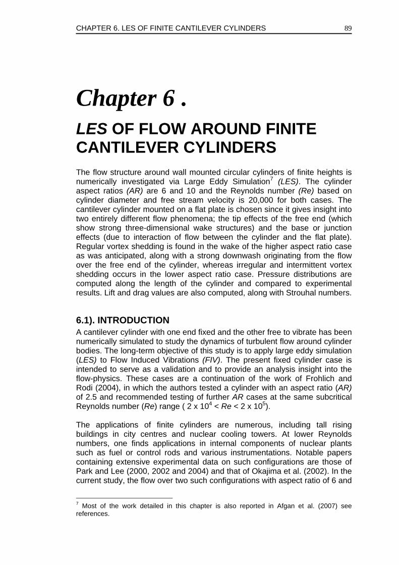
CHAPTER 6. LES OF FINITE CANTILEVER CYLINDERS
89
Chapter 6 . LES OF FLOW AROUND FINITE CANTILEVER CYLINDERS The flow structure around wall mounted circular cylinders of finite heights is numerically investigated via Large Eddy Simulation7 (LES). The cylinder aspect ratios (AR) are 6 and 10 and the Reynolds number (Re) based on cylinder diameter and free stream velocity is 20,000 for both cases. The cantilever cylinder mounted on a flat plate is chosen since it gives insight into two entirely different flow phenomena; the tip effects of the free end (which show strong three-dimensional wake structures) and the base or junction effects (due to interaction of flow between the cylinder and the flat plate). Regular vortex shedding is found in the wake of the higher aspect ratio case as was anticipated, along with a strong downwash originating from the flow over the free end of the cylinder, whereas irregular and intermittent vortex shedding occurs in the lower aspect ratio case. Pressure distributions are computed along the length of the cylinder and compared to experimental results. Lift and drag values are also computed, along with Strouhal numbers.
6.1). INTRODUCTION A cantilever cylinder with one end fixed and the other free to vibrate has been numerically simulated to study the dynamics of turbulent flow around cylinder bodies. The long-term objective of this study is to apply large eddy simulation (LES) to Flow Induced Vibrations (FIV). The present fixed cylinder case is intended to serve as a validation and to provide an analysis insight into the flow-physics. These cases are a continuation of the work of Frohlich and Rodi (2004), in which the authors tested a cylinder with an aspect ratio (AR) of 2.5 and recommended testing of further AR cases at the same subcritical Reynolds number (Re) range ( 2 x 10⁴ < Re < 2 x 10⁵). The applications of finite cylinders are numerous, including tall rising buildings in city centres and nuclear cooling towers. At lower Reynolds numbers, one finds applications in internal components of nuclear plants such as fuel or control rods and various instrumentations. Notable papers containing extensive experimental data on such configurations are those of Park and Lee (2000, 2002 and 2004) and that of Okajima et al. (2002). In the current study, the flow over two such configurations with aspect ratio of 6 and
7 Most of the work detailed in this chapter is also reported in Afgan et al. (2007) see references.
CHAPTER 6. LES OF FINITE CANTILEVER CYLINDERS
90
10 is numerically simulated and then compared to experimental results. A non-conforming local mesh refinement is implemented in all three spatial directions to reduce the size of the computational grid required to resolve the finite cylinder which poses a huge computational grid requirement.
6.2). FLOW GEOMETRY The geometry consists of a finite circular cylinder vertically mounted on a flat plate with one end fixed and the other free (and in later cases also allowed to vibrate, not considered here). The vortices that are shed from the cylinder, along with a strong downwash from its free end require a fairly long computational domain to capture the flow physics adequately. The downstream length is set at 36 diameters and the upstream length is set at 12 diameters, with the origin of the coordinate system located at the centre of the base of the cylinder. The complete geometry is shown in Figure 6-1, where a uniform flow enters from the left. The blockage ratio defined as the ratio of the projected cylinder area to the cross sectional area of test section (A/C) is 1.38 % for AR 6 test case and 2.31% for the AR 10 test case, which is well within the prescribed range for cylinder flows (where the maximum blockage ratio allowed for such flows is 3%; Zdravkovich, 1997). However a little variation in this ratio is still acceptable; Frohlich and Rodi (2004) use a blockage ratio of 7.1% for all their simulations, still achieving decent results as compared to experiments. While understanding the tip flow effects special consideration should also be given to the height of the computational domain. In the present case this total height (HZ) is 24 diameters. Thus the ratio HZ/H = 4 for AR 6 case and 2.4 for AR 10 case which is still sufficiently larger than the experimental (Park and Lee (2000)) ratios of 3.33 and 2 for AR 6 and 10 cases respectively.
6.3). NUMERICAL TREATMENT A prototype8 version of the commercial code STAR-CD V4 is used to solve the 3D Navier-Stokes equations on unstructured grids using a finite volume approach. The flow is assumed to be Newtonian and incompressible. For LES the filtered Navier-Stokes equations are given by;
2 1 ,
0
i i j i ij
j i j j j
i
i
u u u p ut x x x x x
ux
∂ τ∂ ∂ ∂ ∂ν∂ ∂ ρ ∂ ∂ ∂ ∂
∂∂
⎧+ = − + −⎪
⎪⎨⎪ =⎪⎩
(6.1)
8 Simulations started early 2005 using a pre-release made available by CD-adapco, whereas STAR-CD V4 became commercially available in spring 2006. Recent channel and pipe flow LES test cases at Manchester with both versions demonstrated the same results and numerical performance.
CHAPTER 6. LES OF FINITE CANTILEVER CYLINDERS
91
For the subgrid-scale modelling (SGS), the standard Smagorinsky model is used;
2
1 23
2( )
ijij kk ij t
ijS
S
C S S
τ τ δ ν− = −
= − ∆ (6.2)
Where S ij is the filtered strain rate tensor ( S S Sij ij= 2 ). As the cells used in the present work are hexahedral we can take the filter width to be twice that of the cube root of the cell volume ( 1/ 32 olV∆ = ). The Smagorinsky constant9 (CS) is set to 0.065 and is locally damped by a Van Driest wall damping function near solid walls. In the collocated finite volume approach used here, all variables are located at the centres of the cells (which can be of any shape) and the momentum equations are solved by considering an explicit mass flux and a fully centred convection scheme. Pressure-velocity coupling is ensured by a prediction/correction method using the SIMPLE algorithm; Van Doormal and Raithby (1984) also described in Ferziger and Peric (2002). The Poisson equation is solved using a conjugate gradient method. This collocated discretization requires Rhie and Chow (1982) interpolation in the correction step to avoid oscillatory solutions. The three time level implicit time advancing scheme (TTLM) described in Ferziger and Peric (2002), is used for time discretization. This scheme performs the time integration over an interval centered at the new time level and is 2nd order accurate. The non-orthogonalities are taken into account with a reconstruction technique explained in Ferziger and Peric (2002) and are tested for LES by Benhamadouche and Laurence (2003), and Bouris and Bergeles (1999). When a non-orthogonal grid is used, the matrix contains the orthogonal contribution only and the non-orthogonal part is solved explicitly; this is known as the deferred correction. However, one can iterate on the system to make it quasi-implicit. The suitability of this commercial code for LES has been extensively tested at University of Manchester on homogeneous grid turbulence, channel flows and in-line cylinders; Laurence (2006), Moulinec et al. (2005) and Benhamadouche et al. (2005). In Moulinec et al. (2005) the conservation of kinetic energy using collocated unstructured finite volumes was discussed, and a recommended action was to use polyhedral or Cartesian cells with localized refinement rather than a tetrahedral mesh. Conserving kinetic energy not only eliminates numerical diffusion, but also ensures a bounded solution even with pure central differencing schemes, such as those used here. Upwinding, even in small quantity or via higher order terms is not suitable for LES; see Grotzbach and Worner (1999), Kravchenko and Moin (1997).
9 Note the factor 2 in the filter width, i.e. for a cubical cell the filter width is twice the mesh step, as in Moin & Kim (1982) and Pope (2000).
CHAPTER 6. LES OF FINITE CANTILEVER CYLINDERS
92
6.4). GRID DEPENDENCE STUDY A grid independence study was conducted prior to launching the final simulations. For the larger AR case, three meshes were tested, Coarse Non-Conforming Mesh (CNCM1), Fine Non-Conforming Mesh (FNCM1) and a Fine Conforming Mesh (CM). For the smaller AR case, two non-conforming meshes were tested; Coarse Non-Conforming mesh (CNCM2) and Fine Non-Conforming mesh (FNCM2). A list of the five meshes used is given in Table 6-1. The grid generation process was manually controlled to ensure that the overall computational resource requirement was minimized. Thus, the biggest constraint was to limit the grid to be less than 4 million cells in line with available computational resources (8-12 CPUs of an in-house Beowulf cluster). The numerical results from private communications (contributions of Strelets (2005) and Krajnovic (2006) to the DESider database; see acknowledgements) were used for quantitative comparisons in some cases but are not reported in this chapter. The first Strelets (2005) results are based on a grid of 2 million cells for detached eddy simulation (DES). However the present LES grids (FNCM1, CM and FNCM2) in comparison are of the same fineness level near the cylinder surface and flat plate, significantly finer at the tip of the cylinder, but fairly coarse in the far field. This was achieved by use of non-conforming refinement in all directions. The interface cells are not treated as “embedded grids”, but as polyhedral cells with more than 6 faces, i.e. the cell-face based algorithm is the same whatever the number of faces and no special treatment is introduced between regions of different refinement. A total of 9 levels of local refinement have been used with the cell size change ratio limited to a maximum of 33% in every case (i.e. 3 cells matching with 2 cells rather than 2 facing 1 as this latter case has been observed to lead to oscillations in some cases as found by the present study and reported by Laurence, 2006). Thus for every direction the grid has three levels of non-conforming refinements. Figure 6-2 shows a number of views of the computational grids (FNCM1 and CM) with local refinement in different directions. Here the large eddy simulation with near wall resolution (LES-NWR) approach is implemented (Pope, 2000), where the filter and grid are both sufficiently fine to resolve 80% of the energy everywhere. The first cells normal to the cylinder surface along the azimuthal axis are fixed at 1Y + ≈ compared to the 5Y + ≈ for the flat plate which is reasonable enough to model the near wall damping effect. Admittedly this may not be fine enough for an accurate reproduction of boundary layer development, but the boundary layer thickness is fairly short in the experiments ( 6%Dδ ∼ ), since a uniform inlet profile is implemented at the inlet of the flow domain and the distance between the leading edge of the flat plate and the finite cylinder is around 12-16D for both experiments and CFD computations. For the numerical simulations, the side and top surfaces are kept as slip walls to reduce the size of the computational mesh. The solid cylinder surface and the flat bottom plate are treated as no-slip walls. At the inlet, a constant boundary condition with U=U0 (no fluctuations) is prescribed, similar to the experiments (Park and Lee, 2000). At the outlet, a convective outflow
CHAPTER 6. LES OF FINITE CANTILEVER CYLINDERS
93
boundary condition is imposed. These boundary conditions are consistent with those already tested for similar test cases (Frohlich et al., 1998, Frohlich and Rodi, 2004). The LES simulations are run for 20 complete flow cycles, with time averaging of results performed over the last 10 to 12 cycles. Figure 6-3 shows a comparison between the pressure coefficients (CP) obtained from various grids and the experimental data, where (CP) is defined as 2
02( ) /P refC P P Uρ= − . However, as the pressure is variable along the vertical stagnation line, the data has been rescaled with a variable reference pressure Pref(Z) such that 1.0PMaxC ≈ for each altitude (to maintain consistency with the experimental results). Figure 6-3(a) shows the comparison between results from CNCM1, FNCM1 and CM for the higher aspect ratio case (AR 10) at Z/L=0.883. Figure 6-3(b) shows a comparison between results from CNCM2 and FNCM2 for the lower aspect ratio case (AR 6) at Z/L=0.50. For comparison both these figures show the experimental CP profile for an infinite cylinder at the same Re number of 20,000. From Figure 6-3(a) one sees almost no change in the predicted CP profile with the use of CM over FNCM1, demonstrating that the non-conforming cells introduce no adverse effects. With the coarse grid, CNCM1, the negative peak is not fully captured, with a general trend of slightly over predicting pressure in most of the wake side. In Figure 6-3(b) for the lower aspect ratio, the coarser CNCM2 shows the same slight over prediction of wake-side pressure levels as compared to FNCM2 and experiments. The fully conforming mesh is not tested for case 2 since no marked improvement was seen in case 1 with such a mesh, admittedly FNCM2 still slightly under predicts the pressure profile and results in a slightly bigger recirculation region in the wake of the cylinder in both XY and XZ plane. This has been a common observation in all numerical simulations; FNCM1, FNCM2, CM, DES (Strelets, 2005) and very fine LES (Krajnovic, 2006). Thus the finer grids FNCM1 and FNCM2 are chosen for AR 10 and AR 6 test cases respectively and their results are reported in detail in the next section.
6.5). DISCUSSION OF RESULTS
6.5.1). PRESSURE DISTRIBUTION Figure 6-4 shows the vertical mean pressure on the finite cylinder along the stagnation line (0 degrees) and wake line (180 degrees), normalized by the dynamic pressure based on inlet uniform velocity and setting the reference pressure behind the cylinder at the flat plate junction (180 degrees and Z/D=0). The pressure profile at the front is almost constant then drops sharply at - ¼ D from the tip. In Figure 6-4(a) at the back side (1800) near the tip of the cylinder a sharp depression is seen in the pressure profile which corresponds to the vortex core shown in Figure 6-7. It is seen that at - ¼ D from the tip (Z-H = - 0.25 D) a sharp recovery is produced by the backflow below the tip vortex. Then, between - ¼ D to - 3D from the tip, a more gradual recovery is
CHAPTER 6. LES OF FINITE CANTILEVER CYLINDERS
94
observed, resulting from a 3D backflow which is observed from both cross-stream and vertical symmetry plane plots in Figure 6-6 and Figure 6-7. Figure 6-5(a) & (b) shows the mean CP profiles around the cylinder surface for AR 10 (FNCM1) and AR 6 (FNCM2) cases respectively for a number of vertical (Z/L) locations. These CP profiles are in fairly close agreement with the experimental values of Park and Lee (2000 and 2002) up to the minimum located at 70 to 80 degrees. The pressure recovery is slightly slower in the simulations, but the pressure plateau is again well predicted. Beyond 160 degrees the pressure is very much influenced by tip effects. Figure 6-5(a) shows the plots for AR 10 case at Z/L=0.983, Z/L=0.95, Z/L=0.933, Z/L=0.9 and Z/L=0.883 (from top to bottom respectively). The pressure recovery behind the cylinder near the tip is more pronounced, where both experimental and numerical results show this sharp pressure rise in the wake of the cylinder (top left plot in Figure 6-5(a)). The pressure recovery is still visible for Z/L=0.9 which corresponds to -1 D from the tip. However, the downwash effect (which is very strong in the smaller aspect ratio case) is now somewhat reduced, leading to regular vortex shedding in the lower half of the cylinder. For the AR 6 case (Figure 6-5(b)) the profiles are plotted at Z/L=0.983, Z/L=0.944, Z/L=0.917, Z/L=0.806 and Z/L=0.5 (from top to bottom). For this case a fairly stronger downwash is observed which tends to suppress regular vortex shedding in the lower half of the cylinder. Note that for AR 6 case the third graph from top in Figure 6-5(b) which is at Z/L=0.917 and the second graph from the top for AR 10 case in Figure 6-5(a) which is at Z/L=0.95 both correspond to -0.5 D from the tip of the cylinder. Hence the pressure rise due to the tip effect is now much less visible. Experimental findings of Park and Lee (2000, 2002 and 2004) only report such a pressure rise for the aspect ratio 10 case. One can thus conclude, somewhat surprisingly, that the flow structure at the very tip of the cylinder is quite different for AR 6 and AR 10 cases. At Z/L=0.5 the DES results of Strelets (2005) reported in Afgan et al. (2006), the present LES and the ongoing (not shown here) fine LES by (Krajnovic, 2006) tend to show a somewhat higher plateau than the experimental profile in the leeward side of the cylinder. In any case the plateau for all data is significantly higher than that found in the case of an infinite cylinder at similar Reynolds number. This pressure recovery is accompanied by the suppression of vortex shedding behind the cylinder. Experimental findings of Park and Lee (2000) report irregular and weak vortex shedding for the AR 6 case; numerical simulations on the other hand predict intermittent yet barely visible vortex shedding as if the downwash effect is almost strong enough to totally suppress the vortex shedding. For cantilever cylinders, as the aspect ratio decreases the vortex shedding frequency also decreases, but the classification of vortex shedding behind the cylinder depending on the aspect ratio is a debatable issue. Various experimental and numerical results have failed to reach a consensus on the vortex shedding character. According to Farivar (1981), the regular vortex
CHAPTER 6. LES OF FINITE CANTILEVER CYLINDERS
95
shedding disappears for cylinders with an aspect ratio lower than 7.5. Zdravkovich et al. (1989) on the other hand found regular vortex shedding behind a cantilevered cylinder with an aspect ratio of 4. Kawamura et al. (1984) discuss in detail the critical length of a finite cylinder after which vortex shedding is totally suppressed. However, the number of influencing parameters are many: Reynolds number, aspect ratio, blockage effects, approaching boundary layer thickness and free stream or inlet turbulence intensity. While an exact definition of the former three parameters is relatively easy, duplicating the latter two parameters can be somewhat problematic, especially the approaching boundary layer thickness (which itself depends on a number of other parameters such as upstream length, Reynolds number etc.). Hence drawing a clear limiting value of aspect ratio where vortex shedding is totally suppressed is not possible at present, although the current flow is classified to fall into the subcritical regime (2 x 10⁴ < Re < 2 x 10⁵) by Zdravkovich (1997).
6.5.2). VELOCITY DISTRIBUTION Mean velocity streamlines in XY plane for the smaller aspect ratio case (AR 6) are shown in Figure 6-6 at various Z/L locations. It is interesting to note that a pair of narrow recirculation bubbles in the wake generates a strong and wide back-flow (towards the cylinder). This is a significantly different pattern from the infinite cylinder CP plateau shown in Figure 6-3(b). Figure 6-7 shows the streamlines generated from 2D mean velocity vectors in the vertical symmetry plane (Y/D=0). Over the tip of the cylinder the maximum velocity (which at the inlet is 10 m/s) goes as high as 14 m/s. A dense cluster of lines generated just before the tip of the cylinder later highlights the strong arc shaped downstream, almost reaching the base plate. The location of this arc corresponds in Figure 6-6 to the saddle point marking the end of the vortex pair. Thus the streamline divergence along the arc in Figure 6-7 highlights the strong 3D effects and the curved arc shows that the size of the recirculating vortex pair in Figure 6-6 is highly variable with altitude. Hence for the AR 6 cylinder, even at mid height one should not expect results to match closely to that of an infinite cylinder. Near the tip the recirculation (in XZ plane) is much smaller, similar to the findings of Frohlich and Rodi (2004), Kawamura et al. (1984) and Zdravkovich (1997). At the foot of the cylinder, in front, streamlines are seen to curve back towards the plate, just about suggesting a horseshoe vortex but this one is very shallow, as shown in Figure 6-12. Behind the cylinder at the cylinder plate junction a second vortex is seen resulting from the downwash all along the cylinder, but this one is fully embedded in the near wake and is unrelated to the horseshoe vortex. The mean streamwise velocity profile is shown in Figure 6-8 in the wake of the cylinder at two different locations (X/D = 5 and 10). One observes that the higher aspect ratio case (Figure 6-8(a)) has a narrow wake as compared to the smaller case (Figure 6-8 (b)). This is consistent with the fact that with an increasing aspect ratio the flow behaviour becomes that of a 2-D cylinder. Naturally, one would also expect that the effect of the downwash reduces in intensity as one moves away from the cylinder tip both in streamwise
CHAPTER 6. LES OF FINITE CANTILEVER CYLINDERS
96
(downstream) and spanwise directions (along the height of the cylinder). However, this behaviour is quite different for the two cases under consideration. The higher aspect ratio (AR 10) case has a significantly longer recirculation (in XZ plane) bubble and hence the reduction in velocity is not very high near the base of the cylinder at the two monitoring stations (X/D = 5 and 10). This can also be observed with the double velocity peak at Z/H = 0.75 location in Figure 6-8(a). For the smaller aspect ratio (AR 6) case this effect of downwash is more focused along the height of the cylinder rather than its wake, hence a shorter recirculation bubble is observed but with a greater reduction in velocity near the cylinder base. The contour plot of secondary flow 2 2 1/ 2( )v w+ along with average pseudo-streamlines for the AR 10 case (FNCM1) downstream of the cylinder at various X/D locations is shown in Figure 6-9 (this is constructed from the 2-D flow-field in that plane and does not correspond to a projection of 3-D streamlines). Here, pseudo-average streamlines provide a clearer picture of the inverted U of the arch vortices which were discussed earlier. These vortices generated from the tip of the cylinder travel downstream and downwards at the same time vanishing at around 5D downstream of the cylinder (Figure 6-9(d)). It is also observed from the same figure that the effect of these tip vortices travels until a maximum of 2.4D height of the cylinder (also shown as dashed horizontal line shown in Figure 6-9(c)). What is interesting is the heart like shape of the double vortices which, when originated from the tip of the cylinder, are spherical in shape (see Figure 6-9(a)). As they move downstream they are deformed by the strong downwash and the vortex shedding from the sides of the cylinder causing the vortices to converge along the symmetry (Y=0) line thus resulting in perfect heart like shapes (see Figure 6-9(c)). Indeed these structures are a direct consequence of the time averaging of the streamlines and would not have been so clear and well formed in an instantaneous field. For a much smaller cylinder (AR=2.5) Frohlich and Rodi (2004) observed an arched vortex structure in the cylinder’s wake, which is consistent with the well separated vortex pair in Figure 6-9. Investigating the mean vector plots over the tip reveals two counter rotating, oppositely directed, perfectly symmetrical vortices. It is believed that the roll up of the shear flow separation from the free end leads to this counter rotating pair of vortices which later develop into an inverted U structure (as seen in Figure 6-9(a)) causing a strong downwash and thus suppressing the vortex shedding from the sides of the cylinder. Figure 6-9 also signifies the fact that for the larger AR case (AR 10) the effect of the tip vortices is not felt near the base of the cylinder and hence no trace of the tip vortices can be observed on the flat plate. For the smaller AR case (AR 6) the effect is shown to travel up to the base of the cylinder (see Figure 6-7) somewhat similar to what Frohlich and Rodi (2004) observed. Indeed, the smaller AR of 6 of the present simulations and the AR of 4 of Frohlich and Rodi (2004) are quite comparable both in terms of geometric properties
CHAPTER 6. LES OF FINITE CANTILEVER CYLINDERS
97
and flow behaviour. The tip effects in both these cases are seen to be overwhelmingly dominant. Figure 6-10(a) shows the streamlines in XZ symmetry (Y/D=0) plane for the AR 10 case. Here one sees that the recirculation region near the tip of the cylinder is somewhat smaller than the AR 6 case. The instantaneous velocity magnitude plot for the AR 10 case in the XZ plane at Y/L=0 shown in Figure 6-10(b) reveals the vortex columns behind the cylinder which are distorted over 2/3 of the height and even suppressed by the downwash near the tip. Figure 6-11 shows a comparison of velocity magnitudes at Z/L=0.3 (top plots) and Z/L=0.8 (bottom plots) in XY plane. For the smaller aspect ratio case (AR 6, see Figure 6-11(a)) at both Z/L=0.3 and Z/L=0.8 locations, we see a peculiar flow behaviour where the wake splits into two tongues. It is speculated that the strong downwash is directly responsible for this bifurcation of the wake. The phenomenon of classical vortex streets (shedding of one vortex after the other from opposite sides of the cylinder) is being interrupted by the downwash. This causes the flow behaviour on both sides of the cylinder to be independent of each other (unlike a 2-D or infinite 3-D cylinder). However, for the higher aspect ratio case (AR 10, see Figure 6-11(b)) a different flow phenomenon is observed. Here one sees that near the base (at Z/L=0.3) the cylinder wake behaves as a 2-D cylinder with regular vortex shedding from the upper and lower surfaces. Near the tip (at Z/L=0.8) the behaviour is similar to the smaller aspect ratio case. Hence, we conclude that a finite cylinder with aspect ratio 10 shows both finite tip effects and base effects (2-D cylinder behaviour) whereas the aspect ratio 6 cylinder does not show any infinite cylinder behaviour, which extends the findings of Frohlich and Rodi, 2004 from AR 2.5 to AR 6. An instantaneous realization of the 2nd invariant of the velocity gradients for the AR 10 case (FNCM1) is shown in Figure 6-12. For computations, Q is defined as 0.5 ij ij ij ijQ S S⎡ ⎤= − −Ω Ω⎣ ⎦ ; Hunt et al. (1988). Herein it is normalized
as ( 20( / )CQ U Lα= ) where α is a non-dimensional constant set by the user in
order to obtain desired flow structures and CL is the characteristic length scale (in current cases the cylinder diameter). For the current plot the constant α is chosen to return a value of 1Q = s-2. The figure has been rendered by contours vorticity in Z direction ( )zω to show opposite direction of the coherent structures. Near the base of the cylinder we see the trace of the horseshoe vortex as well which is very well defined but was difficult to observe in other instantaneous snapshots. Near the tip of the cylinder the downwash causes a sharp decrease in the turbulence intensity and hence smaller and less structures are seen. Interestingly the Iso-Q structures reveal the difference in the flow behaviour for the two cases. For the AR 6 (see Figure 6-12(a)) one notices some of the larger structures travelling up to the base plate, with a majority of them being concentrated near the base plate. However, for AR 10 case these structures are seen to be shorter in size and more concentrated near the downstream of the wake. Cleary the effect of the
CHAPTER 6. LES OF FINITE CANTILEVER CYLINDERS
98
downwash (which is much stronger for the smaller aspect ratio case) is dictating this flow behaviour. This is further supported by observing Figure 6-12(a) and (b) which show that for the same Iso-Q value the downstream of the cylinder wakes shows a large difference in the mere volume of these coherent structures.
6.5.3). LIFT, DRAG AND TURBULENCE INTENSITY The full three dimensionality of the flow and irregular and intermittent vortex shedding cause highly fluctuating lift (CL) and drag (CD) forces on the cylinder surface (see Figure 6-13(a)), where the coefficients are computed using the projected area (A) of the cylinder and the free stream inlet velocity (Uo). The lift and drag coefficients show a varying amplitude and intensity and hence require substantially long averaging times, similar to the findings of Frohlich and Rodi (2004), but in their case the AR was 2.5 and hence the lift displayed a non-zero local average, forcing them to time average over an even longer period thus making the computations more expensive. The streamwise ( XF ) and normal ( YF ) forces are the sum of the integrated wall pressure and the cylinder surface friction forces, where the contribution of the latter is found to be less than 5% of the total force and hence this friction component is commonly ignored while calculating the streamwise or drag coefficient; Kawamura et al. (1984). Findings of Park and Lee (2000 and 2002) report that the vortex shedding frequency decreases as the aspect ratio of the cylinder decreases where a 2-D cylinder has a Strouhal number of 0.198. A similar trend is seen in the numerical computations, where the Power Spectrum Density analysis (PSD) of the lift coefficient is used to capture the Strouhal numbers for both cases (see Figure 6-13(b)). A comparison between experimental (Park and Lee, 2000, 2002 and 2004) and numerical Strouhal numbers given in Table 6-2 shows a good agreement. To check the degree of accuracy of the numerical results the PSD of AR 10 case was then plotted against the Frequency (Hz) on a log-log scale which is shown in Figure 6-13(c). The slope of the spectrum curve is shown to be in good agreement with a line of -5/3 slope. A comparison between numerically and experimentally obtained mean streamwise turbulence intensity percentage (Tu%) at Z/L=0.5 location in the wake of the cylinder (X/D=5) for the lower aspect ratio case is shown in Figure 6-14. The experimental data taken from Park and Lee (2002) shows a peak value of 28% whereas the LES simulation shows a double peak of 26%. The DES by Strelets (2005) also shows a double peak but with a slightly lower maxima. Interestingly all DESIDER project numerical simulations (DES by Strelets (2005) and very fine LES by Krajnovic (2006), not shown here) predict a double peak for turbulence intensity at this location. This is due to the fact that a slightly longer recirculation region is predicted by all numerical simulations in the wake of the cylinder (as seen in Figure 6-6).
CHAPTER 6. LES OF FINITE CANTILEVER CYLINDERS
99
A comparison of streamwise turbulence intensity u u′ ′< > at various Z/L locations for the higher aspect ratio case is shown in Figure 6-15. One notices that the streamwise turbulence intensities are slightly under-predicted even though the pressure and velocity comparisons were well captured. However, the general trend and the length of the vortex formation region are still predicted accurately. The slight under prediction in numerical results may be attributed to grid coarsening in the wake. The grid has a sufficient resolution near the wall in the wake of the cylinder (Y+=1) but the grid distribution downstream becomes somewhat coarse. Secondly, the Smagorinsky model is not suitable for prediction of laminar to turbulent transition (Figure 6-12 gives some indication that the separating shear layer remains laminar over some distance). We observe that the streamwise turbulence intensities increase while moving towards the fixed end of the cylinder, where the maximum values are behind the lower half of the cylinder (see Figure 6-15). This confirms the initial observation that the effect of the strong down wash is to reduce the turbulence intensity and vortex formation region in the upper half of the cylinder; u u′ ′< > is reduced to almost one third in magnitude (see Figure 6-15). This is confirmed in the experiments and is similar to the observations of Frohlich and Rodi (2004).
6.6). CONCLUSIONS The flow over a cantilever cylinder mounted vertically on a flat plate is numerically simulated by LES for aspect ratios of 6 and 10. Numerical results are compared to experimental data of Park and Lee (2000, 2002 and 2004). The use of multiple levels of local refinements with the STAR-CD code enables the simulation of such a complex geometry using only 2.6 million cells whereas a regular grid LES requirement is at least 10 times higher. Despite the high aspect ratio, the flow over both the cylinders is found to be strongly inhomogeneous along the height of the cylinders, i.e. highly three-dimensional and significantly more turbulent in the lower half of the wake. The roll up of the shear layer separation from the free end causes two counter rotating vortices near the free end of the cylinder leading to a strong downwash extending downstream nearly to the base. This downwash changes the flow evolution by interacting with the regular vortices being shed from the sides of the cylinder. This interaction causes changes in the pressure distribution in the wake of the cylinder and damping of the vortex shedding. For the smaller aspect ratio case the effect of the downwash is stronger, and the tip effect is felt all along the cylinder height. The wake is split into two entirely independent elongated recirculations separated by a large backflow region along the symmetry axis, significantly different from the infinite cylinder case. On the other hand for the higher aspect ratio case the effect of the downwash is limited to the top half of the cylinder and hence the interaction is weaker causing pressure recovery in the wake of the cylinder with regular vortex shedding. The flow pattern at the very tip of the cylinders

CHAPTER 6. LES OF FINITE CANTILEVER CYLINDERS
100
surprisingly changes between AR 6 and 10, with the latter showing stronger pressure recovery due to backflow in the vertical plane. The Strouhal number also shows significant variations. Even for the higher AR, the Cp profile at mid-height is significantly different from that of an infinite cylinder. ACKNOWLEDGEMENTS Author is grateful to C. W. Park and S. J. Lee for provision of experimental data and clarification of its use, as well as discussions with M. Strelets and S. Krajnovic (partners in DESider). This work has been partly supported by DESider project funded by European Union under Contract No. AST3-CT-2003-502842. (http://cfd.me.umist.ac.uk/desider)
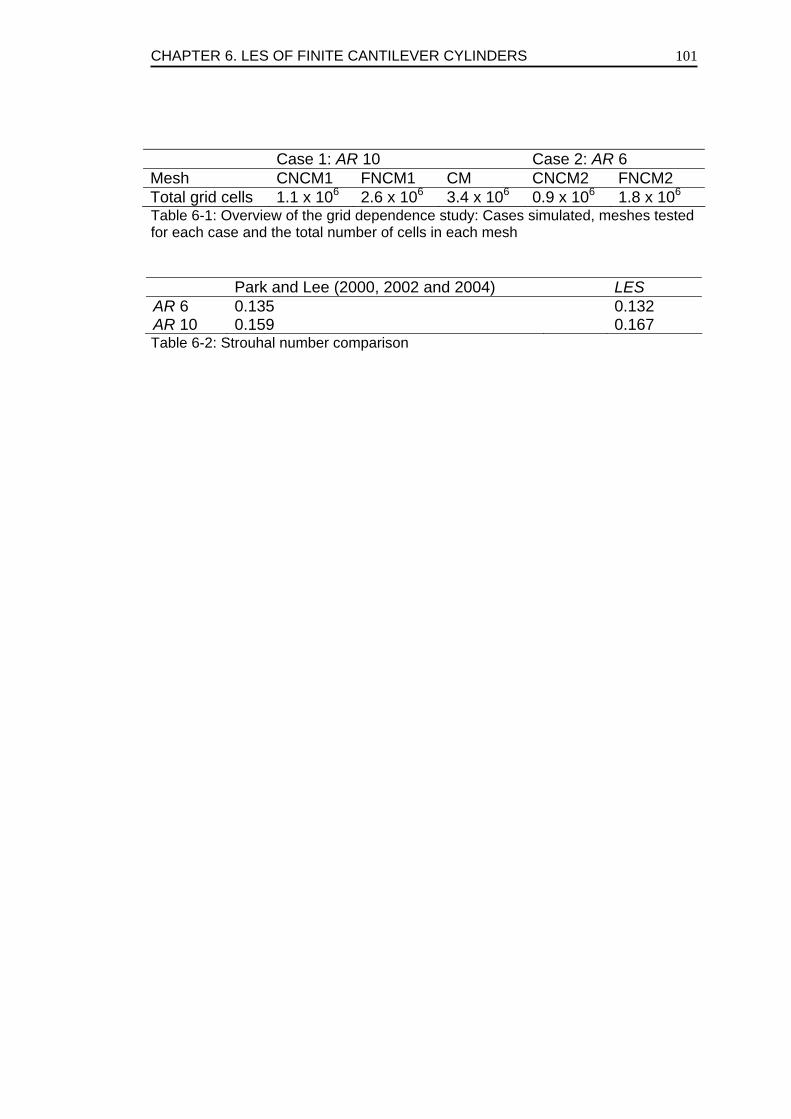
CHAPTER 6. LES OF FINITE CANTILEVER CYLINDERS
101
Case 1: AR 10 Case 2: AR 6 Mesh CNCM1 FNCM1 CM CNCM2 FNCM2 Total grid cells 1.1 x 10⁶ 2.6 x 10⁶ 3.4 x 10⁶ 0.9 x 10⁶ 1.8 x 10⁶ Table 6-1: Overview of the grid dependence study: Cases simulated, meshes tested for each case and the total number of cells in each mesh Park and Lee (2000, 2002 and 2004) LES AR 6 0.135 0.132 AR 10 0.159 0.167 Table 6-2: Strouhal number comparison
CHAPTER 6. LES OF FINITE CANTILEVER CYLINDERS
102
Figure 6-1: Geometry under consideration of finite cylinder. Top: Cross sectional view in XZ plane. Bottom: Cross sectional view in XY plane
CHAPTER 6. LES OF FINITE CANTILEVER CYLINDERS
103
(a) (b)
Figure 6-2: Various orthogonal and sectional views of the grid for AR 10 case. (a): Non-conforming mesh with local refinement (FNCM1). (b): Regular mesh (CM). 3D view of the complete grid (top), sectional view in XZ plane (middle) and sectional view in XY plane (bottom)
CHAPTER 6. LES OF FINITE CANTILEVER CYLINDERS
104
(a) (b)
Figure 6-3: Cp profile around the cylinder. (a): Case1 (AR 10) at Z/L=0.883 (Experiment of Park and Lee (2000), CNCM1, FNCM1 and CM). (b): Case 2 (AR 6) at Z/L=0.5 (Experiment of Park and Lee (2002), CNCM2 and FNCM2)
CHAPTER 6. LES OF FINITE CANTILEVER CYLINDERS
105
(a) (b)
Figure 6-4: Pressure profile along cylinder axis, top: along stagnation line at 0 degrees, bottom: along wake line at 180 degrees. (a): AR 10 case. (b): AR 6 case
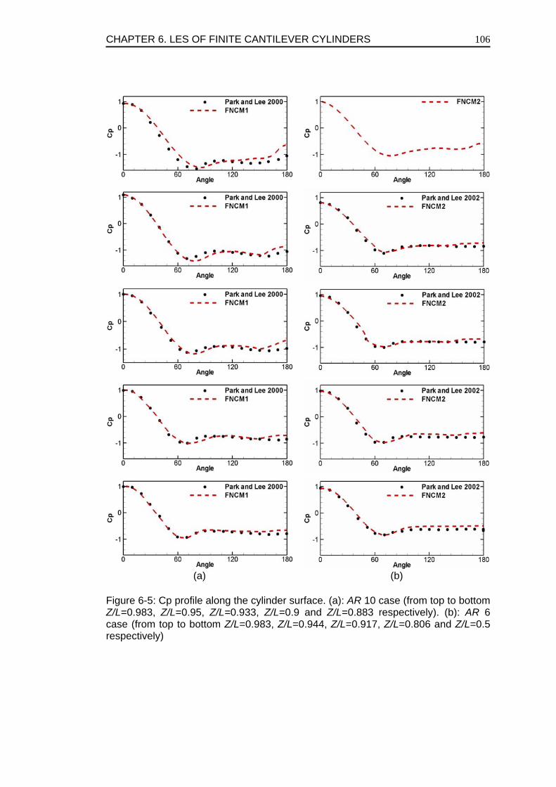
CHAPTER 6. LES OF FINITE CANTILEVER CYLINDERS
106
(a) (b)
Figure 6-5: Cp profile along the cylinder surface. (a): AR 10 case (from top to bottom Z/L=0.983, Z/L=0.95, Z/L=0.933, Z/L=0.9 and Z/L=0.883 respectively). (b): AR 6 case (from top to bottom Z/L=0.983, Z/L=0.944, Z/L=0.917, Z/L=0.806 and Z/L=0.5 respectively)
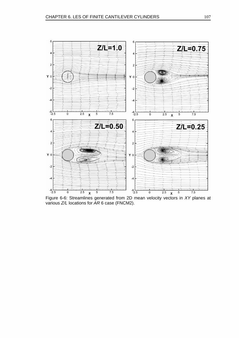
CHAPTER 6. LES OF FINITE CANTILEVER CYLINDERS
107
Figure 6-6: Streamlines generated from 2D mean velocity vectors in XY planes at various Z/L locations for AR 6 case (FNCM2).
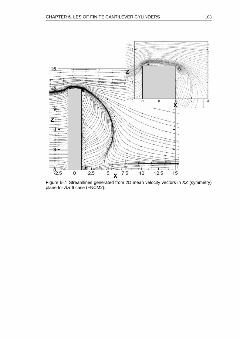
CHAPTER 6. LES OF FINITE CANTILEVER CYLINDERS
108
Figure 6-7: Streamlines generated from 2D mean velocity vectors in XZ (symmetry) plane for AR 6 case (FNCM2).
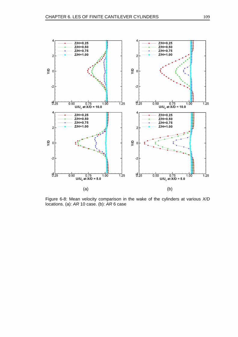
CHAPTER 6. LES OF FINITE CANTILEVER CYLINDERS
109
(a) (b)
Figure 6-8: Mean velocity comparison in the wake of the cylinders at various X/D locations. (a): AR 10 case. (b): AR 6 case
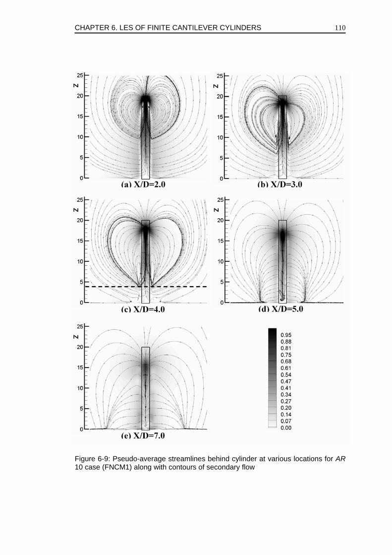
CHAPTER 6. LES OF FINITE CANTILEVER CYLINDERS
110
Figure 6-9: Pseudo-average streamlines behind cylinder at various locations for AR 10 case (FNCM1) along with contours of secondary flow
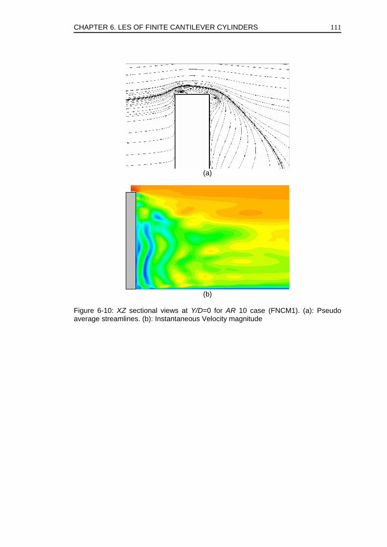
CHAPTER 6. LES OF FINITE CANTILEVER CYLINDERS
111
(a)
(b)
Figure 6-10: XZ sectional views at Y/D=0 for AR 10 case (FNCM1). (a): Pseudo average streamlines. (b): Instantaneous Velocity magnitude
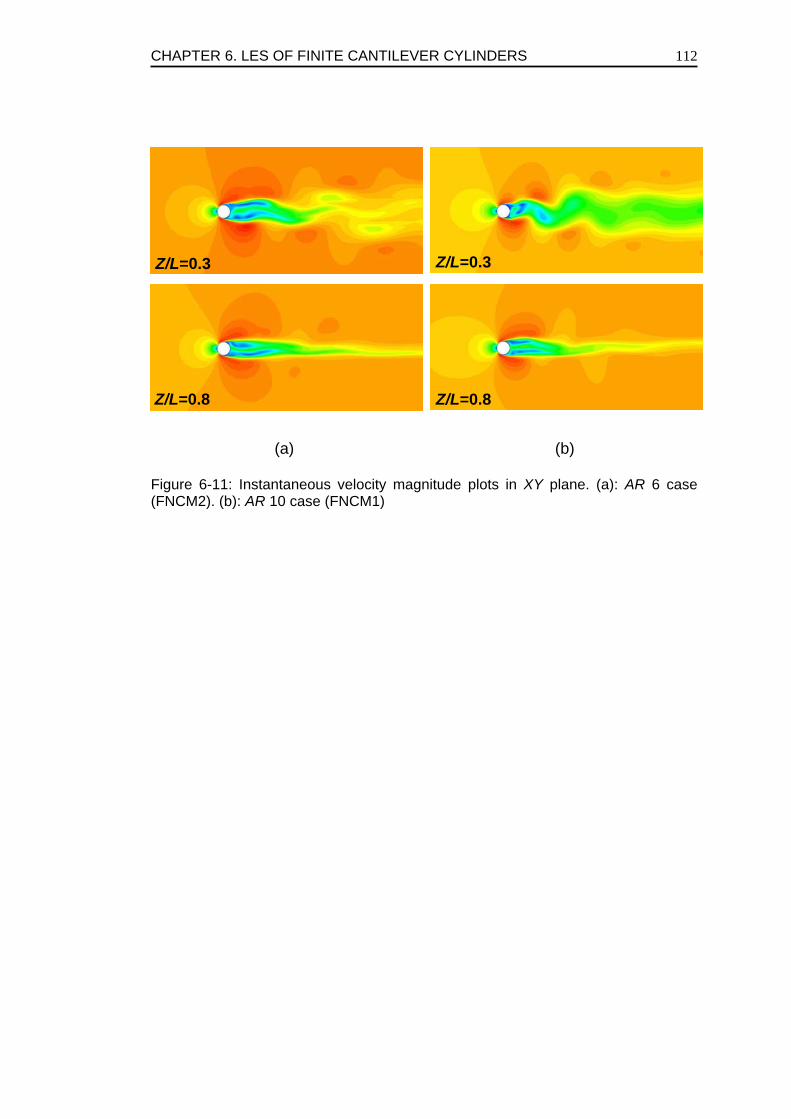
CHAPTER 6. LES OF FINITE CANTILEVER CYLINDERS
112
(a) (b)
Figure 6-11: Instantaneous velocity magnitude plots in XY plane. (a): AR 6 case (FNCM2). (b): AR 10 case (FNCM1)
Z/L=0.3
Z/L=0.8
Z/L=0.3
Z/L=0.8
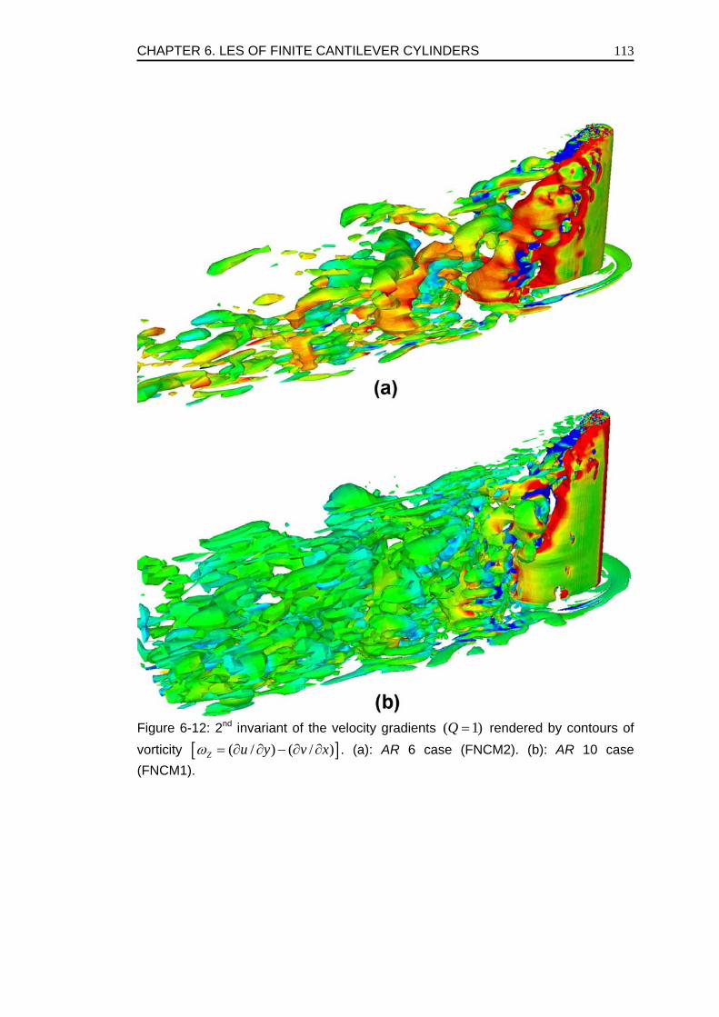
CHAPTER 6. LES OF FINITE CANTILEVER CYLINDERS
113
Figure 6-12: 2nd invariant of the velocity gradients ( 1)Q = rendered by contours of vorticity [ ]( / ) ( / )Z u y v xω = ∂ ∂ − ∂ ∂ . (a): AR 6 case (FNCM2). (b): AR 10 case (FNCM1).
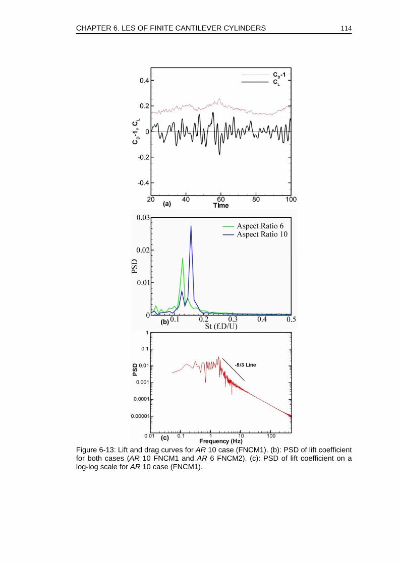
CHAPTER 6. LES OF FINITE CANTILEVER CYLINDERS
114
Figure 6-13: Lift and drag curves for AR 10 case (FNCM1). (b): PSD of lift coefficient for both cases (AR 10 FNCM1 and AR 6 FNCM2). (c): PSD of lift coefficient on a log-log scale for AR 10 case (FNCM1).
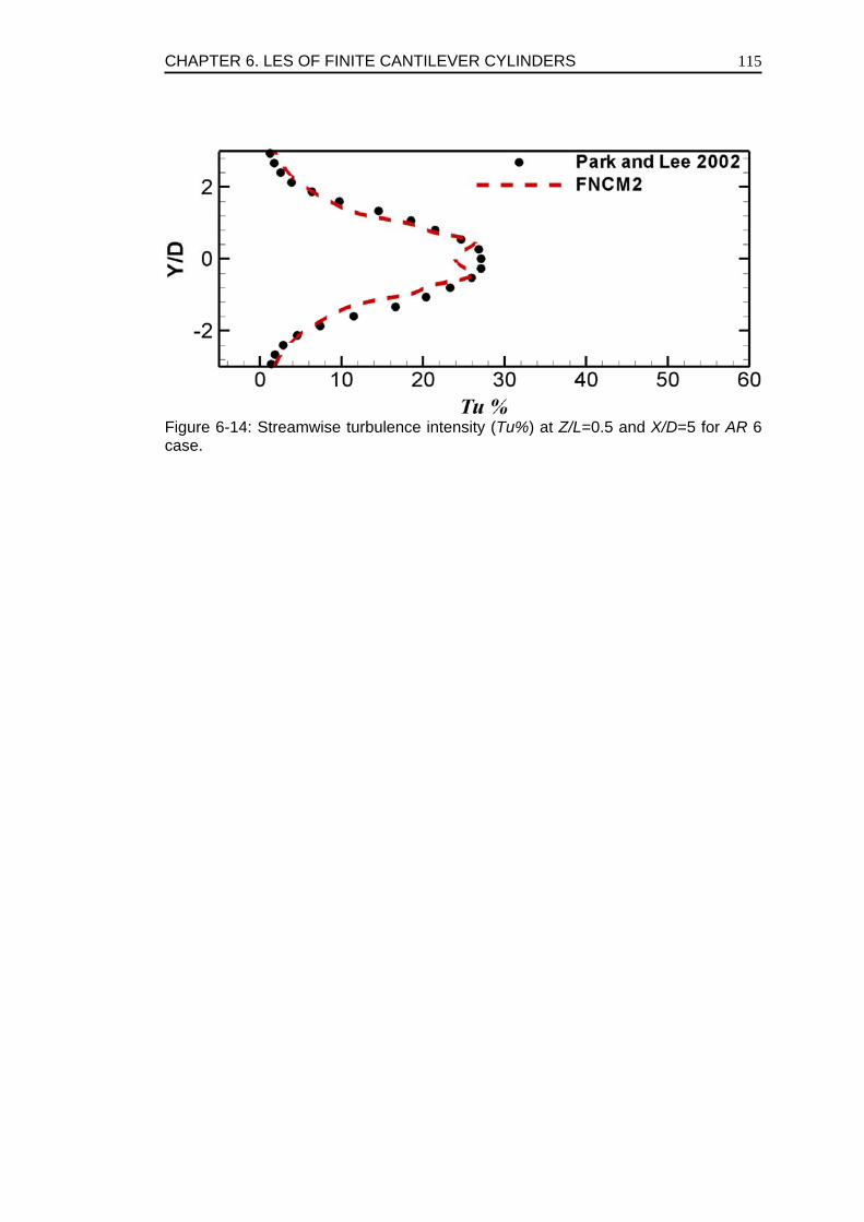
CHAPTER 6. LES OF FINITE CANTILEVER CYLINDERS
115
Figure 6-14: Streamwise turbulence intensity (Tu%) at Z/L=0.5 and X/D=5 for AR 6 case.
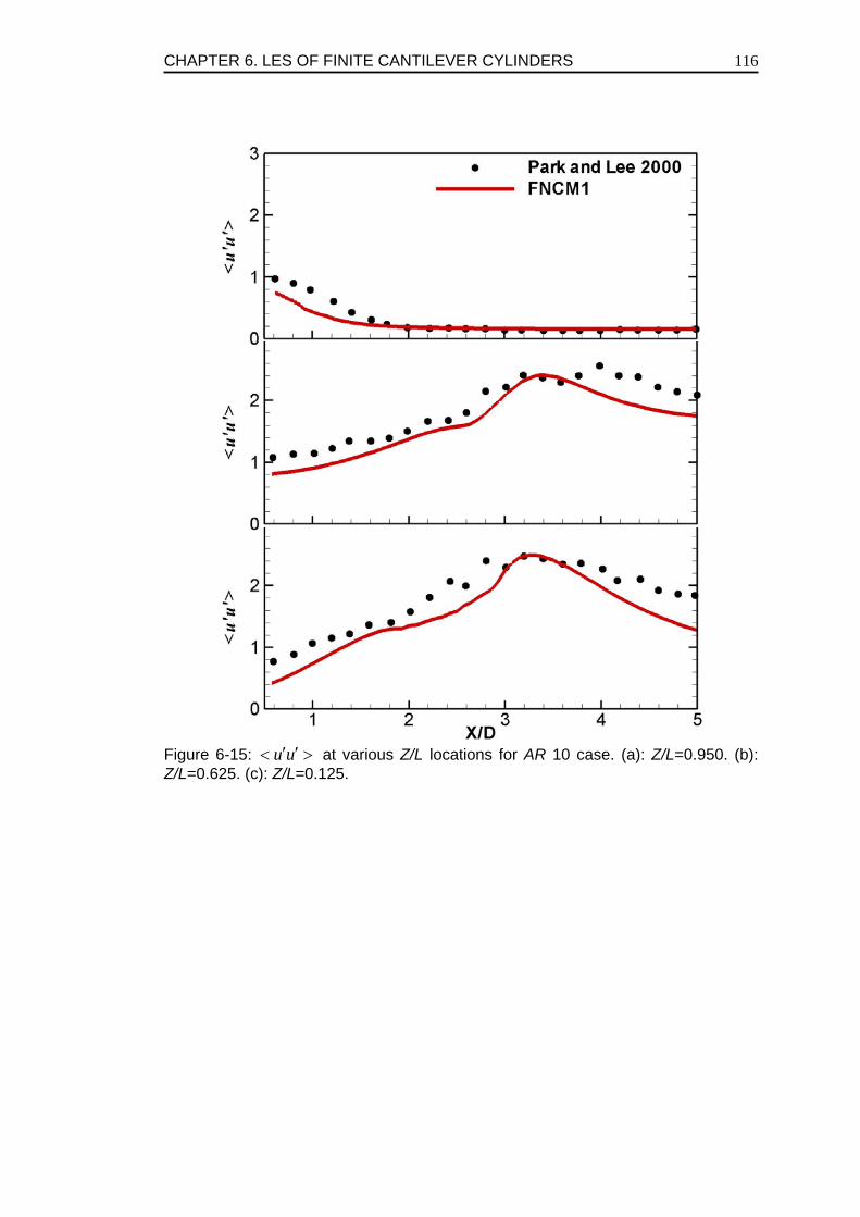
CHAPTER 6. LES OF FINITE CANTILEVER CYLINDERS
116
Figure 6-15: u u′ ′< > at various Z/L locations for AR 10 case. (a): Z/L=0.950. (b): Z/L=0.625. (c): Z/L=0.125.
CHAPTER 6. LES OF FINITE CANTILEVER CYLINDERS
117
BIBLIOGRAPHY Afgan, I., Moulinec, C., Prosser, R., Laurence, D. 2007. Large eddy simulation of turbulent flow for wall mounted cantilever cylinders of aspect ratio 6 and 10. Int. J. Heat Fluid Flow. Article in press, doi:10.1016/j.ijheatfluidflow.2007.04.014. Afgan, I., Moulinec, C., Laurence, D., 2006. Large Eddy Simulation of flow over a vertically mounted finite cylinder on a flat plate. 13th Int. Conf. on Fluid Flow Technologies, CMFF ’06, Budapest, Hungary. 193-200. Benhamadouche, S., Laurence, D., 2003. LES, coarse LES, and transient RANS comparisons on the flow across tube bundle. Int. J. Heat and Fluid Flow. 4, 470-479. Benhamadouche, S., Laurence, D., Jarrin, N., Afgan, I., Moulinec, C., 2005. Large Eddy Simulation of flow across in-line tube bundles. NURETH-11, Avignon, France. Bouris, D., Bergeles, G., 1999. Two dimensional time dependent simulation of the subcritical flow in a staggered tube bundle using a Subgrid scale model. Int. J. Heat and Fluid Flow. 20(2), 105-114. Farivar, D. 1981. Turbulent uniform flow around cylinders of finite length. J. of AIAA J. 19, 275-281. Ferziger, J. H., Peric, M., 2002. Computational Methods for Fluid Dynamics. Springer, 3rd edition. Frohlich, J., Rodi, W., Kessler, P., Parpais, S., Bertoglio, J., Laurence, D., 1998. Large Eddy Simulation of flow over circular cylinders on structured and unstructured grids. In: Hirschel, E. (Ed.), Numerical Flow Simulation I. In: Notes on Numerical Fluid Mechanics, vol. 66. Vieweg, pp. 319-338. Frohlich, J., Rodi, W., 2004. LES of flow around a circular cylinder of finite height. Int. J. of Heat and Fluid Flow. 25, 537-548.
CHAPTER 6. LES OF FINITE CANTILEVER CYLINDERS
118
Grotzbach, G., Worner, M., 1999. Direct numerical and large eddy simulations in nuclear applications. Int. J. of Heat and Fluid Flow. 20, 222-240. Hunt, J. C. R., Wray, A. A., Moin, P., 1988. Eddies, stream and convergence zones in turbulent flows. Report CTR-S88. Center for Turbulent Research. Kawamura, T., Hiwada, M., Hibino, T., Mabuchi, I., Kamuda, M., 1984. Flow around a finite circular cylinder on a flat plate. Bull. JSME 27 (232), 2142-2151. Krajnovic, S. 2006. Private communications (results and publications available on http://cfd.me.umist.ac.uk/desider). Kravchenko, A. G., Moin, P., 1997. On the effect of numerical errors in large eddy simulation of turbulent flows. J. Comp. Phys. 131, 310-322. Laurence, D., 2006. Large Eddy Simulation with unstructured finite volumes. In "Direct and Large-Eddy Simulation VI", Lamballais, E., Friedrich, R., Geurts, B.J., Métais, O. (Eds.), Springer ERCOFTAC series 10, 27-38. Moin, P., Kim, J., 1982. Numerical investigation of turbulent channel flow. J. Fluid Mech. 118, 341–377. Moulinec, C., Benhamadouche, S., Laurence, D., Peric, M., 2005. LES in a U-bend pipe meshed by polyhedral cells. ERCOFTAC ETMM-6 conference, Sardinia, Elsevier. Okajima, A., Kosugi, T., Nakamura, A., 2002. Flow-induced in-line oscillation of a circular cylinder in a water tunnel. J. Press. Vess. Tech. ASME 124, 89-96. Park, C. W., Lee, S. J., 2000. Free end effect on the wake flow structure behind a finite circular cylinder. J. Wind Eng. Ind. Aero. 88, 231-246. Park, C. W., Lee, S. J., 2002. Flow structure around a finite circular cylinder embedded in various atmospheric boundary layers. Fluid Dyn. Res. 30, 197-215.
CHAPTER 6. LES OF FINITE CANTILEVER CYLINDERS
119
Park, C. W., Lee, S. J., 2004. Effects of free-end corner shape on flow structure around a finite cylinder. J. Fluids Struct. 19, 141-158. Pope, S. B., 2000. Turbulent Flows. Cambridge university press, 1st edition. Rhie, C., Chow, W., 1982. A numerical study of the flow past an isolated airfoil with trailing edge separation. AIAA J. 21, 1525–1532. Strelets, M. 2005. Private communications (results and publications available on http://cfd.me.umist.ac.uk/desider). Van Doormal, J.P., Raithby, G.D., 1984. Enhancements of the SIMPLE method for predicting incompressible fluid flows. Num. Heat Transfer 7, 147-163. Zdravkovich, M. M., Brand, V. P., Mathew, G., and Weston, A., 1989. Flow past short circular cylinders with two ends free. J. Fluid Mech. 203, 557-575. Zdravkovich, M., 1997. Flow Around Circular Cylinders. Oxford University Press.
CHAPTER 7. IN-LINE TUBE BUNDLES
120
Chapter 7 .
REVIEW OF FLOW IN IN-LINE TUBE BUNDLES
7.1). INTRODUCTION In the previous chapters we discussed some aspects of the flow over single finite cylinders. However, in the current chapter we shall consider clusters of densely packed cylinders called tube bundles. These arrays of tubes can be arranged in in-line (straight), staggered (rotated squared), normal triangle or parallel (rotated normal triangular) configurations. Our particular interest is in the in-line configuration as this is widely used in heat exchangers of chemical and nuclear/coal power plants. For a single cylinder the transition from laminar to turbulent flow is immediate following the flow over the body and is directly related to the Reynolds number and inlet turbulence levels. However, for closely packed tube bundles the interstitial flow generates turbulence row after row until the dissipation is balanced by production and a statistically steady fully developed turbulent flow field is generated. To make matters even more complicated the wake and proximity interference of the cylinders play a direct role in the development of the flow physics thereby making the flow highly complex and difficult to numerically investigate. In the current chapter we shall limit our discussion to various experimental and numerical efforts spent in understanding such flows. However, in the next few chapters we shall show numerical results obtained by LES for a wide range of gap ratios followed by a detailed comparison made with RANS modelling.
7.2). LITERATURE REVIEW OF FLOW IN TUBE BUNDLES Much like single cylinders the tube response inside tube bundles is also highly prone to oscillations. The turbulence and periodic excitation by coherent vorticity phenomenon may lead to severe vibrations thus causing extensive damage to tube bundles over a short period of time. Cylinder clusters in cross-flow have periodic vortex shedding which lead to forced vibrations, if these vibrations are close to the natural frequency of cylinders the result could lead to a catastrophic failure of the structure. It is thus to this task that we turn to; investigate the literature review in relation to tube response to vortex shedding and cylinder vibrations.
CHAPTER 7. IN-LINE TUBE BUNDLES
121
7.2.1). LIFT AND DRAG COEFFICIENTS Placing a cylinder in the wake of another, changes the physics of the flow. The downstream cylinder behavior is now dependent upon the flow pattern in the wake of the upstream cylinder. Arie et al. (1983) showed that for a tandem arrangement the fluctuating lift and drag on the down stream cylinder is strongly dependent upon the gap spacing. It was shown that as the gap spacing increases, the fluctuating forces also increase. It was concluded by the authors that the worst case scenario is at a gap distance of 4.5 D, where the fluctuating forces on the downstream cylinder are the maximum. Tatsuno et al. (1991) perform a similar experimental study on the stable posture of a pair of parallel cylinders in uniform flow. The cylinder pair was allowed to move about the mid point of the line joining their centers. The gap distances were varied and the stable position was observed when the cylinder pair was released at various angles of attack. It was observed that when P/D is 0.5, because of proximity interference the cylinders came to rest in side by side arrangement ( 090α = ) at zero angle of attack, when the P/D ratio was 1.0 and 1.5 the pair was stable in both tandem ( 00α = ) and side by side arrangement ( 090α = ). However, when the gap ratio is 2.0 or more, the proximity interference almost vanishes and the cylinders become stable only in tandem arrangement ( 00α = ). Sayers (1988) did a wind tunnel study of four equidistant cylinders subjected to various inflow inclination angles, spacing ratios were also varied from 1.1 to 5 for a Reynolds number of 30,000. The staggered arrangement at an inclination angle of 45 degrees becomes in-line. For this in-line arrangement it was seen that at a spacing ratio of 1.5 the drag force was the highest, suggesting clearly that the drag of an in-line array is far more than the drag of a staggered arrangement. Lift forces on the other hand fluctuates more or less around a zero value for all inclination angles. Chen (1972) and Pettigrew and Ko (1980) contains extensive data for lift and drag for various tube bundle configurations; in-line, triangular and staggered arrangements. Most of the data used in the subsequent chapters will be taken from these studies where extensive numerical (LES and RANS) comparisons will be made for a wide range of gap ratios. There are some other interesting configurations which are also of particular interest such as Wu et al. (2002) in which a cylinder is placed behind another one but with a little offset from the centre line. The upstream cylinder is always fixed whereas the downstream cylinder is tested at various positions to see which configuration results in small lift and drag forces. The idea behind this study was to find an optimal location for the downstream cylinder to cater the needs of risers in marine engineering. It is concluded that the down stream cylinder will always have a non-zero lift and drag.
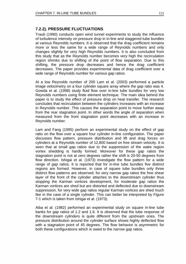
CHAPTER 7. IN-LINE TUBE BUNDLES
122
7.2.2). PRESSURE FLUCTUATIONS Traub (1990) conducts open wind tunnel experiments to study the influence of turbulence intensity on pressure drop in in-line and staggered tube bundles at various Reynolds numbers. It is observed that the drag coefficient remains more or less the same for a wide range of Reynolds numbers and only changes slightly for very high Reynolds numbers. It is also concluded from this study that as the Reynolds number becomes very high the recirculation region shrinks due to shifting of the point of flow separation. Due to this shifting, the pressure drop decreases and hence the drag coefficient decreases. The paper provides experimental data of drag coefficient over a wide range of Reynolds number for various gap ratios. At a low Reynolds number of 200 Lam et al. (2003) performed a particle image velocimetry on a four cylinder square array where the gap ratio was 4. Gowda et al. (1998) study fluid flow over in-line tube bundles for very low Reynolds numbers using finite element technique. The main idea behind the paper is to study the effect of pressure drop on heat transfer. The research concludes that recirculation between the cylinders increases with an increase in Reynolds number. This causes the separation point to move further away from the rear stagnation point. In other words the angle of separation when measured from the front stagnation point decreases with an increase in Reynolds number. Lam and Fang (1995) perform an experimental study on the effect of gap ratio on the flow over a square four cylinder in-line configuration. The paper discusses flow pattern, pressure distribution and lift and drag forces on cylinders at a Reynolds number of 12,800 based on free stream velocity. It is seen that at small gap ratios due to the suppression of the wake region vortex shedding is hardly formed. Moreover for these gap ratios the stagnation point is not at zero degrees rather the shift is 20-50 degrees from flow direction. Ishigai et al. (1973) investigate the flow pattern for a wide range of gap ratios. It is reported that for in-line tube bundles five distinct regions are formed. However, in case of square tube bundles only three distinct flow patterns are observed; for very narrow gap ratios the free shear layer of the front of the cylinder attaches to the downstream cylinder thus stopping the Karman vortices development, for moderate gap ratios the Karman vortices are shed but are distorted and deflected due to downstream suppression, for very wide gap ratios regular Karman vortices are shed much like in the case of a single cylinder. This can better be interpreted by Figure 7-1 which is taken from Ishigai et al. (1973). Aiba et al. (1982) performed an experimental study on square in-line tube banks for gap ratios of 1.2 and 1.6. It is observed that the tube response of the downstream cylinders is quite different from the upstream ones. The pressure distribution around the cylinder surface shows highly deflected flow with a stagnation point of 45 degrees. The flow behavior is asymmetric for both these configurations which is owed to the narrow gap ratios.
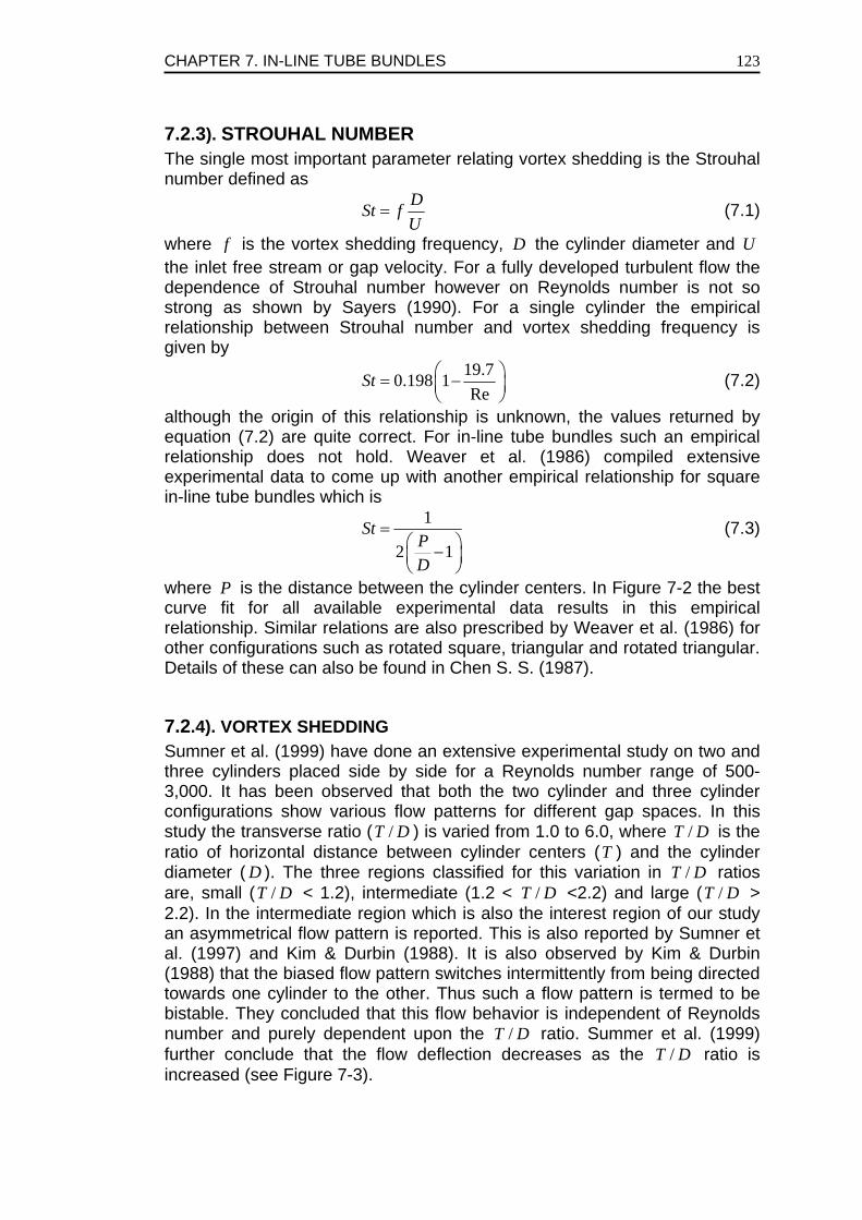
CHAPTER 7. IN-LINE TUBE BUNDLES
123
7.2.3). STROUHAL NUMBER The single most important parameter relating vortex shedding is the Strouhal number defined as
DSt fU
= (7.1)
where f is the vortex shedding frequency, D the cylinder diameter and U the inlet free stream or gap velocity. For a fully developed turbulent flow the dependence of Strouhal number however on Reynolds number is not so strong as shown by Sayers (1990). For a single cylinder the empirical relationship between Strouhal number and vortex shedding frequency is given by
19.70.198 1Re
St ⎛ ⎞= −⎜ ⎟⎝ ⎠
(7.2)
although the origin of this relationship is unknown, the values returned by equation (7.2) are quite correct. For in-line tube bundles such an empirical relationship does not hold. Weaver et al. (1986) compiled extensive experimental data to come up with another empirical relationship for square in-line tube bundles which is
1
2 1St
PD
=⎛ ⎞−⎜ ⎟⎝ ⎠
(7.3)
where P is the distance between the cylinder centers. In Figure 7-2 the best curve fit for all available experimental data results in this empirical relationship. Similar relations are also prescribed by Weaver et al. (1986) for other configurations such as rotated square, triangular and rotated triangular. Details of these can also be found in Chen S. S. (1987).
7.2.4). VORTEX SHEDDING Sumner et al. (1999) have done an extensive experimental study on two and three cylinders placed side by side for a Reynolds number range of 500-3,000. It has been observed that both the two cylinder and three cylinder configurations show various flow patterns for different gap spaces. In this study the transverse ratio ( /T D ) is varied from 1.0 to 6.0, where /T D is the ratio of horizontal distance between cylinder centers (T ) and the cylinder diameter ( D ). The three regions classified for this variation in /T D ratios are, small ( /T D < 1.2), intermediate (1.2 < /T D <2.2) and large ( /T D > 2.2). In the intermediate region which is also the interest region of our study an asymmetrical flow pattern is reported. This is also reported by Sumner et al. (1997) and Kim & Durbin (1988). It is also observed by Kim & Durbin (1988) that the biased flow pattern switches intermittently from being directed towards one cylinder to the other. Thus such a flow pattern is termed to be bistable. They concluded that this flow behavior is independent of Reynolds number and purely dependent upon the /T D ratio. Summer et al. (1999) further conclude that the flow deflection decreases as the /T D ratio is increased (see Figure 7-3).
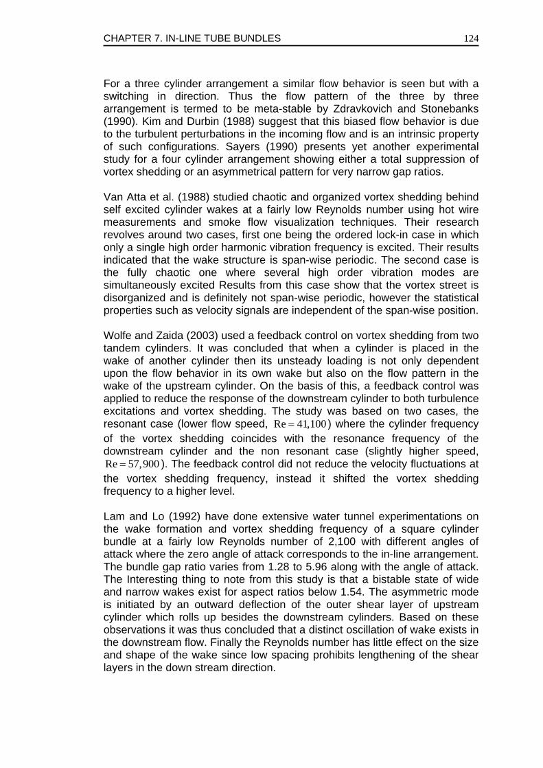
CHAPTER 7. IN-LINE TUBE BUNDLES
124
For a three cylinder arrangement a similar flow behavior is seen but with a switching in direction. Thus the flow pattern of the three by three arrangement is termed to be meta-stable by Zdravkovich and Stonebanks (1990). Kim and Durbin (1988) suggest that this biased flow behavior is due to the turbulent perturbations in the incoming flow and is an intrinsic property of such configurations. Sayers (1990) presents yet another experimental study for a four cylinder arrangement showing either a total suppression of vortex shedding or an asymmetrical pattern for very narrow gap ratios. Van Atta et al. (1988) studied chaotic and organized vortex shedding behind self excited cylinder wakes at a fairly low Reynolds number using hot wire measurements and smoke flow visualization techniques. Their research revolves around two cases, first one being the ordered lock-in case in which only a single high order harmonic vibration frequency is excited. Their results indicated that the wake structure is span-wise periodic. The second case is the fully chaotic one where several high order vibration modes are simultaneously excited Results from this case show that the vortex street is disorganized and is definitely not span-wise periodic, however the statistical properties such as velocity signals are independent of the span-wise position. Wolfe and Zaida (2003) used a feedback control on vortex shedding from two tandem cylinders. It was concluded that when a cylinder is placed in the wake of another cylinder then its unsteady loading is not only dependent upon the flow behavior in its own wake but also on the flow pattern in the wake of the upstream cylinder. On the basis of this, a feedback control was applied to reduce the response of the downstream cylinder to both turbulence excitations and vortex shedding. The study was based on two cases, the resonant case (lower flow speed, Re 41,100= ) where the cylinder frequency of the vortex shedding coincides with the resonance frequency of the downstream cylinder and the non resonant case (slightly higher speed, Re 57,900= ). The feedback control did not reduce the velocity fluctuations at the vortex shedding frequency, instead it shifted the vortex shedding frequency to a higher level. Lam and Lo (1992) have done extensive water tunnel experimentations on the wake formation and vortex shedding frequency of a square cylinder bundle at a fairly low Reynolds number of 2,100 with different angles of attack where the zero angle of attack corresponds to the in-line arrangement. The bundle gap ratio varies from 1.28 to 5.96 along with the angle of attack. The Interesting thing to note from this study is that a bistable state of wide and narrow wakes exist for aspect ratios below 1.54. The asymmetric mode is initiated by an outward deflection of the outer shear layer of upstream cylinder which rolls up besides the downstream cylinders. Based on these observations it was thus concluded that a distinct oscillation of wake exists in the downstream flow. Finally the Reynolds number has little effect on the size and shape of the wake since low spacing prohibits lengthening of the shear layers in the down stream direction.
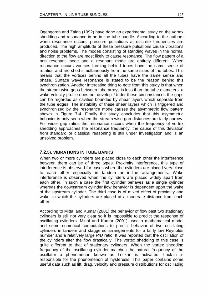
CHAPTER 7. IN-LINE TUBE BUNDLES
125
Ogengoren and Zaida (1992) have done an experimental study on the vortex shedding and resonance in an in-line tube bundle. According to the authors when resonance occurs, pressure pulsations at discrete frequencies are produced. The high amplitude of these pressure pulsations cause vibrations and noise problems. The modes consisting of standing waves in the normal direction to the flow are most likely to cause resonance. The flow pattern of a non resonant mode and a resonant mode are entirely different. When resonance occurs vortices forming behind tubes have the same sense of rotation and are shed simultaneously from the same sides of the tubes. This means that the vortices behind all the tubes have the same sense and phase. Surface wave resonance is stated to be the reason behind this synchronization. Another interesting thing to note from this study is that when the stream-wise gaps between tube arrays is less than the tube diameters, a wake velocity profile does not develop. Under these circumstances the gaps can be regarded as cavities bounded by shear layers which separate from the tube edges. The instability of these shear layers which is triggered and synchronized by the resonance mode causes the asymmetric flow pattern shown in Figure 7-4. Finally the study concludes that this asymmetric behavior is only seen when the stream-wise gap distances are fairly narrow. For wider gap ratios the resonance occurs when the frequency of vortex shedding approaches the resonance frequency, the cause of this deviation from standard or classical reasoning is still under investigation and is an unsolved problem.
7.2.5). VIBRATIONS IN TUBE BANKS When two or more cylinders are placed close to each other the interference between them can be of three types. Proximity interference, this type of interference is observed for cases where the cylinders are placed very close to each other especially in tandem or in-line arrangements. Wake interference is observed when the cylinders are placed widely apart from each other. In such a case the first cylinder behaves as a single cylinder whereas the downstream cylinder flow behavior is dependent upon the wake of the upstream cylinder. The third case is of mixed effect of proximity and wake, in which the cylinders are placed at a moderate distance from each other. According to Mittal and Kumar (2001) the behavior of flow past two stationary cylinders is still not very clear so it is impossible to predict the response of oscillating cylinders. Mittal and Kumar (2001) used a mathematical model and some numerical computations to predict behavior of two oscillating cylinders in tandem and staggered arrangements for a fairly low Reynolds number and a relatively large P/D ratio. It was reported that the oscillation of the cylinders alter the flow drastically. The vortex shedding of this case is quite different to that of stationary cylinders. When the vortex shedding frequency of the oscillating cylinder matches the natural frequency of the oscillator a phenomenon known as Lock-in is activated. Lock-in is responsible for the phenomenon of hysteresis. This paper contains some useful data such as lift, drag, velocity and pressure distributions for oscillating
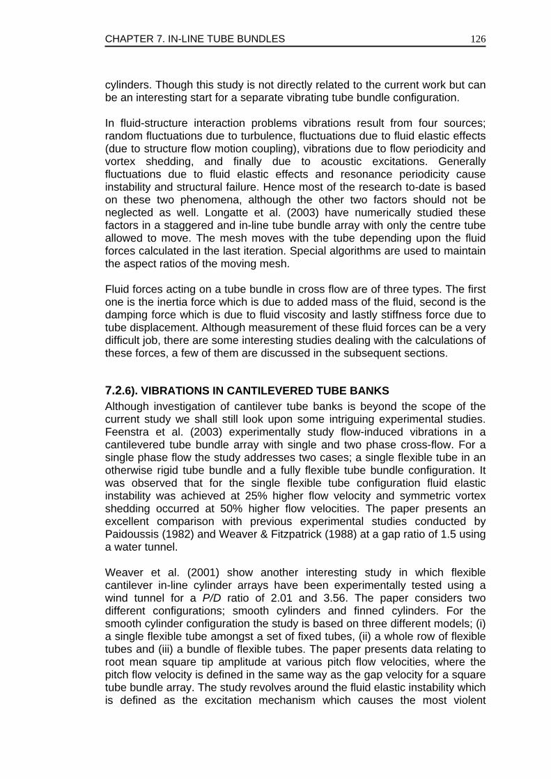
CHAPTER 7. IN-LINE TUBE BUNDLES
126
cylinders. Though this study is not directly related to the current work but can be an interesting start for a separate vibrating tube bundle configuration. In fluid-structure interaction problems vibrations result from four sources; random fluctuations due to turbulence, fluctuations due to fluid elastic effects (due to structure flow motion coupling), vibrations due to flow periodicity and vortex shedding, and finally due to acoustic excitations. Generally fluctuations due to fluid elastic effects and resonance periodicity cause instability and structural failure. Hence most of the research to-date is based on these two phenomena, although the other two factors should not be neglected as well. Longatte et al. (2003) have numerically studied these factors in a staggered and in-line tube bundle array with only the centre tube allowed to move. The mesh moves with the tube depending upon the fluid forces calculated in the last iteration. Special algorithms are used to maintain the aspect ratios of the moving mesh. Fluid forces acting on a tube bundle in cross flow are of three types. The first one is the inertia force which is due to added mass of the fluid, second is the damping force which is due to fluid viscosity and lastly stiffness force due to tube displacement. Although measurement of these fluid forces can be a very difficult job, there are some interesting studies dealing with the calculations of these forces, a few of them are discussed in the subsequent sections.
7.2.6). VIBRATIONS IN CANTILEVERED TUBE BANKS Although investigation of cantilever tube banks is beyond the scope of the current study we shall still look upon some intriguing experimental studies. Feenstra et al. (2003) experimentally study flow-induced vibrations in a cantilevered tube bundle array with single and two phase cross-flow. For a single phase flow the study addresses two cases; a single flexible tube in an otherwise rigid tube bundle and a fully flexible tube bundle configuration. It was observed that for the single flexible tube configuration fluid elastic instability was achieved at 25% higher flow velocity and symmetric vortex shedding occurred at 50% higher flow velocities. The paper presents an excellent comparison with previous experimental studies conducted by Paidoussis (1982) and Weaver & Fitzpatrick (1988) at a gap ratio of 1.5 using a water tunnel. Weaver et al. (2001) show another interesting study in which flexible cantilever in-line cylinder arrays have been experimentally tested using a wind tunnel for a P/D ratio of 2.01 and 3.56. The paper considers two different configurations; smooth cylinders and finned cylinders. For the smooth cylinder configuration the study is based on three different models; (i) a single flexible tube amongst a set of fixed tubes, (ii) a whole row of flexible tubes and (iii) a bundle of flexible tubes. The paper presents data relating to root mean square tip amplitude at various pitch flow velocities, where the pitch flow velocity is defined in the same way as the gap velocity for a square tube bundle array. The study revolves around the fluid elastic instability which is defined as the excitation mechanism which causes the most violent
CHAPTER 7. IN-LINE TUBE BUNDLES
127
vibrations leading to rapid tube failure. The flow velocity at which this failure occurs is termed as critical or threshold velocity. Price and Paidoussis (1989) investigate a single flexible cylinder placed inside a rigid tube bundle configuration with a gap ratio of 1.5. Data for this case corresponds gap velocities and turbulence intensities.
7.3). INVESTIGATION OF FLOW IN TUBE BANKS VIA NUMERICAL SIMULATIONS Numerical simulation of flow in a three dimensional tube bundle requires extensive computational resources especially for high Reynolds number flows, according to Avisar et al. (2001) only a few such computations have been attempted to date. Benhamadouche and Laurence (2003) discuss cross flow in a staggered tube bundle array with different levels of grid refinement. It has been stated both by this study and by Rollet-Miet et al. (1999) that standard 2 equations RANS models fail to produce reliable results for flow inside tube bundles. Rollet-Miet et al. (1999) suggest that for LES there is little difference in results between the Smagorinsky and the Dynamic Smagorinsky models. Based on this conclusion Benhamadouche and Laurence (2003) used a Smagorinsky model, a centered convection scheme and the SIMPLEC method for pressure and velocity coupling. The Reynolds number based on bulk velocity was 9,000, whereas the Y + for the fine LES mesh was less than 7. It is stated that the flow occasionally switches direction and can take a 45 degree orientation, a phenomenon which also frequently appears in in-line tube bundle configurations. Findings report that the high levels of fluctuations are due to oscillations of the flow around cylinder. The future work suggested by this paper is to test an in-line tube bundle with slightly displaced central cylinder. Rollet-Miet et al. (1999) used a finite element code for LES and RANS of a staggered tube bundle array. The Reynolds number chosen for this study is 16,000 based on bulk velocity and gap ratio variation is between 1.5 and 4. Both Smagorinsky and Dynamic Smagorinsky models have been tested and it was concluded that dynamic model has no advantage over Smagorinsky model for this case except at some locations (stagnation points). For time discretization Crank Nicholson scheme was used and the Smagorinsky constant was set at 0.065. For the LES case an element cell is chosen and is shown that no coherent large structures are generated due to imposing periodicity in small domains. It is also stated that for a tube bundle case in regions of high turbulent intensity Reynolds number is expected to have little influence on the flow. DNS of similar tube bundles is Moulinec et al. (2003) in which a staggered array is tested with P/D variation from 2 to 3. The cases are tested for very low Reynolds number (less than 6,000). The interesting thing is that the study tries to explain a lot of unanswered questions regarding tube bundles. Questions such as what is the sufficient domain size needed for a numerical
CHAPTER 7. IN-LINE TUBE BUNDLES
128
simulation? What is the flow transition Reynolds number from 2-D to 3-D? What is the effect of gap spacing on flow behavior? In Moulinec et al. the time discretization was performed by Adams-Bashforth scheme and spatial discretizations were performed using second order central differencing scheme. It was concluded that in staggered tubes vortex shedding appears at a Reynolds number of 125 as opposed to a single cylinder case where shedding appears at a Reynolds number of 40. It was also concluded that for the single cylinder case the flow becomes turbulent at Reynolds number of 2000 whereas in this case the Reynolds number was found to be 6,000. Finally it is found that at for this Reynolds number due to increased turbulent dispersion of the wake vorticity, wake disappearance occurs. Barsamian and Hassan (1997) have performed an LES study of cross-flow in square arrangement of in-line and staggered tube bundles with P/D ratio of 1.95. Two SGS models have been used; the Smagorinsky model and a modified Smagorinsky model which caters for Leonard and cross terms. For both the cases the Smagorinsky constant was fixed at 0.075 and the Reynolds number based on gap velocity was varied from 13,300 to 53,300. The study is basically two dimensional but it was concluded on the basis of Hassan and Lee (1993) that the velocity and force time history have similar results as those of a three dimensional case. Other data contained in this paper relates to lift and drag forces. As expected the instantaneous lift fluctuates around the zero mark thus resulting in an almost mean zero lift. Apart from cylinder bundles some research has also been carried out on in-line square cylinder bundles. One such paper worth mentioning is Cheng et al. (2003) in which a matrix of in-line cubes have been tested by various numerical simulations including k ε− , Smagorinsky, dynamic Smagorinsky and Localized dynamic model at a Reynolds number of 3,800 based on bulk velocity. The study concludes that qualitative results of all the numerical schemes including k ε− model compare quite well. However, quantitatively the k ε− model over predicts the separation region. On the other hand predictions obtained with the Smagorinsky model are off by only a few percent. It is also noted that the use of the Dynamic model leads to additional unphysical backscatter of energy for which various cures have to be thought of in the future. For LES cases spatial discretizations are carried out using second order central differencing scheme and the time discretization using Crank-Nicholson scheme. Finally it was concluded that although complex features like vortex shedding and separation zones are predicted better with LES, the cost of computation increases significantly.
CHAPTER 7. IN-LINE TUBE BUNDLES
129
Figure 7-1: Flow pattern in in-line tube bundles taken from Ishigai et al. (1973), where P is the horizontal distance between tube centers and T is the vertical distance
CHAPTER 7. IN-LINE TUBE BUNDLES
130
Figure 7-2: Strouhal number for square cylinder arrays against gap ratios taken from Weaver et al. (1986)
CHAPTER 7. IN-LINE TUBE BUNDLES
131
Figure 7-3: Picture taken from Sumner et al. (1999) showing biased deflection angle against T/D for two cylinders
1.0 1.5 2.0 2.5 3.0 3.5
T/D
CHAPTER 7. IN-LINE TUBE BUNDLES
132
Figure 7-4: Picture taken from Ogengoren and Zaida (1992), showing biased flow pattern for a resonant case
CHAPTER 7. IN-LINE TUBE BUNDLES
133
BIBLIOGRAPHY Aiba, S., Tsuchida, H., Ota, T. 1982. Heat transfer around tubes in in-line tube banks. Bull JSME, 25. 919-926; in Flow around circular cylinders Vol 2:Applications by Zdravkovich, M. M. Arie, M., Kiya, M., Moriya, M., Mori, H. 1983. Pressure fluctuations on the surface of two cylinders in tandem arrangement. J. Fluids Eng. 105. PP. 161-167. Avisar, B., Shemer, L., Kribus, A. 2001. Measurements of velocity fields in finite cylinder arrays with and without tip clearance. Exp. Thermal Fluid Science. 24. 157-167. Barsamian, H. R., Hassan, Y. A. 1997. Large eddy simulation of turbulent cross-flow in tube bundles. Nucl. Eng. Design, 172. 103-122. Benhamadouche, S., Laurence, D. R. 2003. LES, coarse LES, and transient RANS comparisons on the flow across a tube bundle. Int. J. Heat Fluid Flow. 24. 470-479. Chen, Y. N. 1972. Fluctuating lift forces of the Karman vortex streets on single cylinders and tube bundles, part 3 - Lift forces in tube bundles. Trans. ASME, J. Engg. for Industry 94, 603-628;in Flow induced vibration of circular cylinder structures by Chen, S. S. Cheng, Y., Lien, F. S., Yee, E., Sinclair, R. 2003. A comparison of large eddy simulations with a standard k- Reynolds averaged Navier-Stokes model for the prediction of a fully developed turbulent flow over a matrix of cubes. J. Wind Eng. Ind. Aero. 91. 1301-1328. Feenstra, P. A., Weaver, D. S., Nakamura, T. 2003. Vortex shedding and fluidelastic instability in a normal square tube array excited by two-phase cross-flow. J. Fluids Struct. 17. 793-811. Gowda, Y. T. K., Narayana, P. A. A., Seetharamu, K. N. 1998. Finite element analysis of mixed convection over in-line tube bundles. Int. J. Heat Mass Transfer. Vol. 41, No. 11, pp. 1613-1619. Hassan, Y. A., Lee, S. Y. 1993. Application of Large Eddy Simulation to Three-Dimensional Tube bundle flows, NURETH-6, 2. PP. 1415-1419. Ishigai, S., Nishikawa, E., Yagi, E. 1973. Structures of Gas flow and vibration in tube banks with tube axes normal to flow. Inst. Sym. on Marine Engineering, Tokyo. PP. 1-5-23 to 1-5-33; in Flow induced vibration of circular cylinder structures by Chen, S. S.
CHAPTER 7. IN-LINE TUBE BUNDLES
134
Kim, H. J., Durbin, P. A. 1988. Investigation of the flow between a pair of circular cylinders in the flopping regime. J. Fluid Mech. 196. 431-448. Lam, K., Fang, X. 1995. The effect of interference of four equispaced cylinders in cross flow on pressure and force coefficients. J. Fluids Struct.. 9. 195-214. Lam, K., Li, J. Y.,Chan, K. T., So, R. M. C. 2003. Flow pattern and velocity field distribution of cross-flow around four cylinders in a square configuration at a low Reynolds number. J. Fluids Struct. 17. 665-679. Lam, K., Lo, S. C. 1992. A visualization study of cross flow around four cylinders in a square configuration. J. Fluids Struct. 6. 109-131. Longatte, E., Bendjeddou, Z., Souli, M. 2003. Methods for numerical study of tube bundle vibrations in cross-flow. J. Fluids Struct. 18. 513-528. Mittal, S., Kumar, V. 2001. Flow induced oscillations of two cylinders in tandem and staggered arrangements. J. Fluids Struct. 15. 717-736. Moulinec, C., Hunt, J. C. R., Nieuwstadt, F. T. M. 2003. Disappearing wakes and dispersion in numerically simulated flows through tube bundles. Klumwer Academic Publishers. 23-27. Ogengoren A., Zaida, S. 1992. Vorticity shedding and acoustic resonance in an In-line tube bundle, Part II: Acoustic resonance. J. Fluids Struct. 6. PP. 293-309. Paidoussis, M. P. 1982. A review of flow induced vibrations in reactors and reactor components. Nucl. Eng. Design. Vol 74. 31-60. Pettigrew, M. J., Ko, P. L. 1980. A comprehensive approach to avoid vibration on fretting in shell and tube heat exchangers. Flow induced vibration of power plant components, PVP-41, ASME publications, pp. 1-18; in Flow induced vibration of circular cylinder structures by Chen, S. S. Price, S. J., Paidoussis, M. P. 1989. The flow induced response of a single flexible cylinder in an in-line array of rigid cylinders. J. of Fluids and Structures, 3. 61-82; in Flow around circular cylinders Vol 2: Applications by Zdravkovich, M. M. Rollet-Miet, P., Laurence, D. R., Ferziger, J. 1999. LES and RANS of turbulent flow in tube bundles. Int. J. Heat Fluid Flow. 20. 241-254. Sayers, A. T. 1988. Flow interference between four equispaced cylinders when subjected to a cross flow. J. Wind Eng. Ind. Aero. 31. 9-28.
CHAPTER 7. IN-LINE TUBE BUNDLES
135
Sayers, A. T. 1990. Vortex shedding from groups of three and four equispaced cylinders situated in cross flow. J. Wind Eng. Ind. Aero. 34. 213-221. Sumner, D., Wong, S. S. T., Price, S. J., Paidoussis, M., P. 1997. Two and three side by side circular cylinders in steady cross-flow. Proceedings of the 16th Canadian Congress of Applied Mechanics, Vol 1. pp. 273-274. Sumner, D., Wong, S. S. T., Price, S. J., Paidoussis, M., P. 1999. Fluid behavior of side by side circular cylinders in steady cross-flow. J. Fluids Struct. 13. 309-338. Tatsuno, M., Amamoto, H., Ishi-i, K. 1991. On a stable posture of a pair of parallel cylinders in a uniform flow. Fluid Dyn. Res. 8. 253-272. Traub, D. 1990. Turbulent heat transfer and pressure drop in plain tube bundles. Chem. Eng. Process. 28. 173-181. Van Atta, C. W., Gharib, M., Hammache, M. 1988. Three dimensional structure of ordered and chaotic vortex streets behind circular cylinders at low Reynolds numbers. Fluid Dyn. Res. 3. 127-132. Weaver, D. S., Fitzpatrick, J. A. 1988. A review of cross flow induced vibrations in heat exchanger tube arrays. J Fluids Struct. 2. 73-93. Weaver, D. S., Fitzpatrick, J. A., Elkashlan, H. 1986. Strouhal numbers for heat exchanger tube arrays in cross flow. Flow induced vibrations, PVP Vol. 104. ASME Publications; in Flow induced vibration of circular cylinder structures by Chen, S. S. Weaver, D. S., Zaida, S., Sun, Z., Feenstra, P. 2001. The effect of platen fins on the flow induced vibrations of an in-line tube array. ASME, PVP-Vol 420-1, pp. 91-100. Wolfe, D., Zaida, S. 2003. Feedback control of vortex shedding from two tandem cylinders. J. Fluids Struct. 17 579-592. Wu, W., Huang, S., Barltrop, N. 2002. Current induced instability of two circular cylinders. Applied Ocean Research 24. 287-297. Zdravkovich, M. M. and Stonebanks, K. L. 1990. Intrinsically non-uniform and meta-stable flow in and behind tube arrays. J. Fluids and Struct. 4. 305-319.
CHAPTER 8. LES OF TUBE BUNDLES
136
Chapter 8 . LES OF FLOW IN TUBE BUNDLES The heat transfer and power generation industrial sector is showing much interest in the numerical simulation of cross-flow in tube bundle arrays. Indeed, such a numerical tool could allow a systematic study of numerous configurations including various gap to diameter ratios and numerous angles of flow directions with respect to tube alignments. Extensive experimental study is limited by the difficulty of accessing the complete inter-tube region obviously, and is too costly to be used as design optimisation. It is also too incomplete to understand complex phenomenon such as flow induced vibrations, particle deposition and two phase flow generally. Prior to LES simulations, some 2-D simulations were run, but the results were not found to be very satisfactory. Four gap ratios (P/D) of square in-line tube bundles are tested; 1.2, 1.5, 1.6 and 1.75. For the three smaller gap ratios the flow is found to be bistable with asymmetrical behaviour. However, for the wider gap ratio of 1.75 the flow is intrinsically stable and perfectly symmetrical. Two-point correlation tests lead to the conclusion that one needs a minimum extrusion length of 2 diameters in the spanwise or homogeneous direction to accommodate the use of periodic boundary conditions. Lift and drag coefficients and their root mean square (r.m.s) values are computed from LES and are found to be in good agreement with the experimental data.
8.1). INTRODUCTION The applications of tube bundles are vast and many from industrial heat exchangers to coal and nuclear power generation systems. Hence there are many issues that need to be addressed and resolved properly. One such concern is the strong fluid-structure coupling which acts as a cyclic load on tubes inside the heat exchangers. These cyclic loadings in time cause extensive wear and in some cases might even lead to catastrophe such as the sodium leak due to damage in the fast breeder reactor of “Monju” in Japan in 199510. In fluid structure problems, vibrations result from four sources; random fluctuations due to turbulence, fluctuations due to fluid elastic effects (structure flow motion coupling), resonance due to flow
10 http://www.ieer.org/reports/npd7.html
CHAPTER 8. LES OF TUBE BUNDLES
137
periodicity leading to vortex shedding, and finally due to acoustic excitations. Generally, fluctuations due to fluid-elastic effects and resonance periodicity cause instability and structural failure. Hence flow-induced vibrations of bluff bodies occurring in industrial plants have been of great interest for many decades. The need for a major parametric CFD study of tube bundles would seem timely and worthwhile especially when seen from the point of view of the billion dollars per year potential savings worldwide for coal power plants alone (Bouris et al., 2001). CFD simulations using Reynolds Averaged Navier Stokes (RANS) equations for staggered tube bundle cases have so far not produced any reliable results, this has been extensively reported in numerous studies: the ERCOFTAC workshops on refined flow modelling of 1993 and 1994, Rollet-Miet et al. (1999), Sebag et al. (1991), Meyer (1994), and Bouris and Bergeles (1999). These discrepancies have led researchers to turn to LES, which has allowed an accurate analysis of stress loading, heat transfer and deposition rates which are highly dependent on the turbulence intensities. Numerous reported studies including that of Rollet-Miet et al. (1999) and Benhamadouche and Laurence (2003) have successfully applied LES to tube bundle flows and obtained quite reasonable results. Rollet-Miet et al. (1999) also suggests that for a staggered arrangement there is little or no difference between results obtained with the standard Smagorinsky or the Dynamic Smagorinsky model, although the same inference cannot be deduced for an in-line configuration without extensive numerical testing.
8.2). NUMERICAL TREATMENT In the present case, in-line tube bundles are tested with various gap ratios using the standard Smagorinsky model. Some 2-D simulations are also performed prior to 3-D LES. Both quantitative and qualitative results are then analyzed and compared to understand the complex flow phenomenon in in-line tube bundles. The flow is assumed to be Newtonian and incompressible. For the subgrid-scale modelling (SGS), the standard Smagorinsky model as shown in Chapter 6 is used. Since the cells used in the present work are hexahedral, the filter width is taken twice that of the cube root of the cell volume ( 1/ 32 olV∆ = ). The Smagorinsky constant (CS) is set to 0.065 and is locally damped by a Van Driest wall damping function near solid walls. To obtain the desired bulk velocity a self-correcting mean pressure gradient is specified at every time step. This is done by adding a source term to the momentum equation which is given by
1
11 1
( ) 0.5( )n nref refn n
z
Q Q Q QF F
tL hρ
−+ − − −= +
∆ (8.1)
Where n is the time step, 1F the source term (homogeneous to a pressure gradient) in conjunction with the timestep, Q is the volume flux calculated in a chosen plane of the computational domain (the first periodic plane in the streamwise direction for example) and refQ is the imposed volume flux. Such an approach has been successfully implanted in the past for both channel
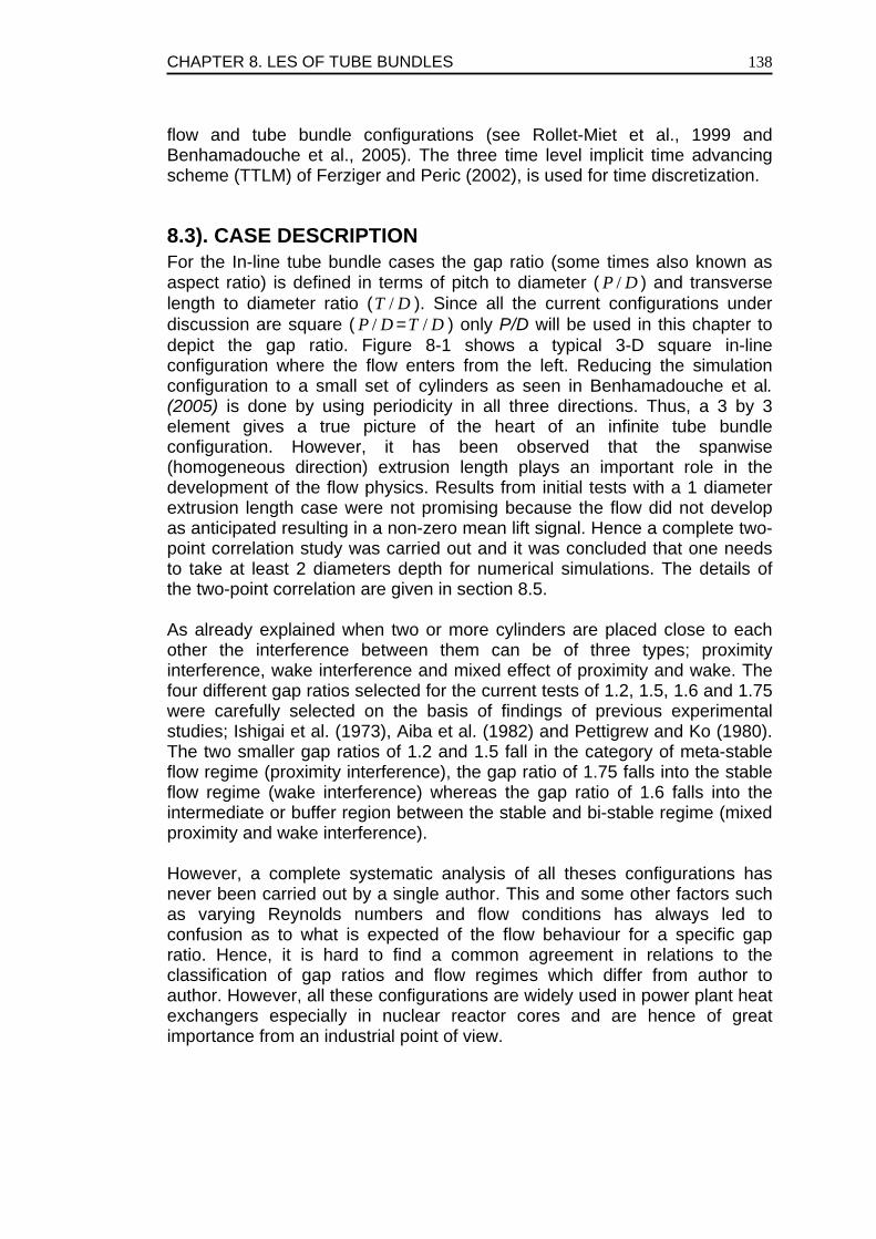
CHAPTER 8. LES OF TUBE BUNDLES
138
flow and tube bundle configurations (see Rollet-Miet et al., 1999 and Benhamadouche et al., 2005). The three time level implicit time advancing scheme (TTLM) of Ferziger and Peric (2002), is used for time discretization.
8.3). CASE DESCRIPTION For the In-line tube bundle cases the gap ratio (some times also known as aspect ratio) is defined in terms of pitch to diameter ( /P D ) and transverse length to diameter ratio ( /T D ). Since all the current configurations under discussion are square ( /P D = /T D ) only P/D will be used in this chapter to depict the gap ratio. Figure 8-1 shows a typical 3-D square in-line configuration where the flow enters from the left. Reducing the simulation configuration to a small set of cylinders as seen in Benhamadouche et al. (2005) is done by using periodicity in all three directions. Thus, a 3 by 3 element gives a true picture of the heart of an infinite tube bundle configuration. However, it has been observed that the spanwise (homogeneous direction) extrusion length plays an important role in the development of the flow physics. Results from initial tests with a 1 diameter extrusion length case were not promising because the flow did not develop as anticipated resulting in a non-zero mean lift signal. Hence a complete two-point correlation study was carried out and it was concluded that one needs to take at least 2 diameters depth for numerical simulations. The details of the two-point correlation are given in section 8.5. As already explained when two or more cylinders are placed close to each other the interference between them can be of three types; proximity interference, wake interference and mixed effect of proximity and wake. The four different gap ratios selected for the current tests of 1.2, 1.5, 1.6 and 1.75 were carefully selected on the basis of findings of previous experimental studies; Ishigai et al. (1973), Aiba et al. (1982) and Pettigrew and Ko (1980). The two smaller gap ratios of 1.2 and 1.5 fall in the category of meta-stable flow regime (proximity interference), the gap ratio of 1.75 falls into the stable flow regime (wake interference) whereas the gap ratio of 1.6 falls into the intermediate or buffer region between the stable and bi-stable regime (mixed proximity and wake interference). However, a complete systematic analysis of all theses configurations has never been carried out by a single author. This and some other factors such as varying Reynolds numbers and flow conditions has always led to confusion as to what is expected of the flow behaviour for a specific gap ratio. Hence, it is hard to find a common agreement in relations to the classification of gap ratios and flow regimes which differ from author to author. However, all these configurations are widely used in power plant heat exchangers especially in nuclear reactor cores and are hence of great importance from an industrial point of view.
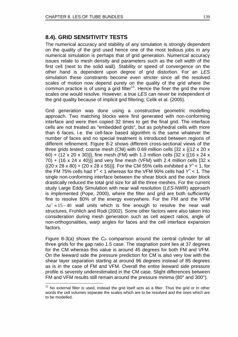
CHAPTER 8. LES OF TUBE BUNDLES
139
8.4). GRID SENSITIVITY TESTS The numerical accuracy and stability of any simulation is strongly dependent on the quality of the grid used hence one of the most tedious jobs in any numerical simulation is perhaps that of grid generation. Numerical accuracy issues relate to mesh density and parameters such as the cell width of the first cell (next to the solid wall). Stability or speed of convergence on the other hand is dependent upon degree of grid distortion. For an LES simulation these constraints become even stricter since all the resolved scales of motion now depend purely on the quality of the grid where the common practice is of using a grid filter11. Hence the finer the grid the more scales one would resolve. However, a true LES can never be independent of the grid quality because of implicit grid filtering; Celik et al. (2005). Grid generation was done using a constructive geometric modelling approach. Two matching blocks were first generated with non-conforming interface and were then copied 32 times to get the final grid. The interface cells are not treated as “embedded grids”, but as polyhedral cells with more than 6 faces, i.e. the cell-face based algorithm is the same whatever the number of faces and no special treatment is introduced between regions of different refinement. Figure 8-2 shows different cross-sectional views of the three grids tested; coarse mesh (CM) with 0.69 million cells [32 x (12 x 20 x 60) + (12 x 20 x 30)], fine mesh (FM) with 1.3 million cells [32 x (16 x 24 x 70) + (16 x 24 x 40)] and very fine mesh (VFM) with 2.4 million cells [32 x (20 x 28 x 80) + (20 x 28 x 55)]. For the CM 55% cells exhibited a Y+ < 1, for the FM 75% cells had Y+ < 1 whereas for the VFM 90% cells had Y+ < 1. The single non-conforming interface between the shear block and the outer block drastically reduced the total grid size for all the three meshes. For the current study Large Eddy Simulation with near wall resolution (LES-NWR) approach is implemented (Pope, 2000), where the filter and grid are both sufficiently fine to resolve 80% of the energy everywhere. For the FM and the VFM
15 40z+∆ ≈ − wall units which is fine enough to resolve the near wall structures, Frohlich and Rodi (2002). Some other factors were also taken into consideration during mesh generation such as cell aspect ratios, angle of non-orthogonalities, warp angles for faces and the cell interface expansion factors. Figure 8-3(a) shows the CP comparison around the central cylinder for all three grids for the gap ratio 1.5 case. The stagnation point lies at 37 degrees for the CM whereas this value is around 45 degrees for both FM and VFM. On the leeward side the pressure prediction for CM is also very low with the shear layer separation starting at around 96 degrees instead of 85 degrees as is in the case of FM and VFM. Overall the entire leeward side pressure profile is severely underestimated in the CM case. Slight differences between FM and VFM results still remain around the pressure minima (80° and 300°). 11 No external filter is used, instead the grid itself acts as a filter. Thus the grid or in other words the cell volumes separate the scales which are to be resolved and the ones which are to be modelled.
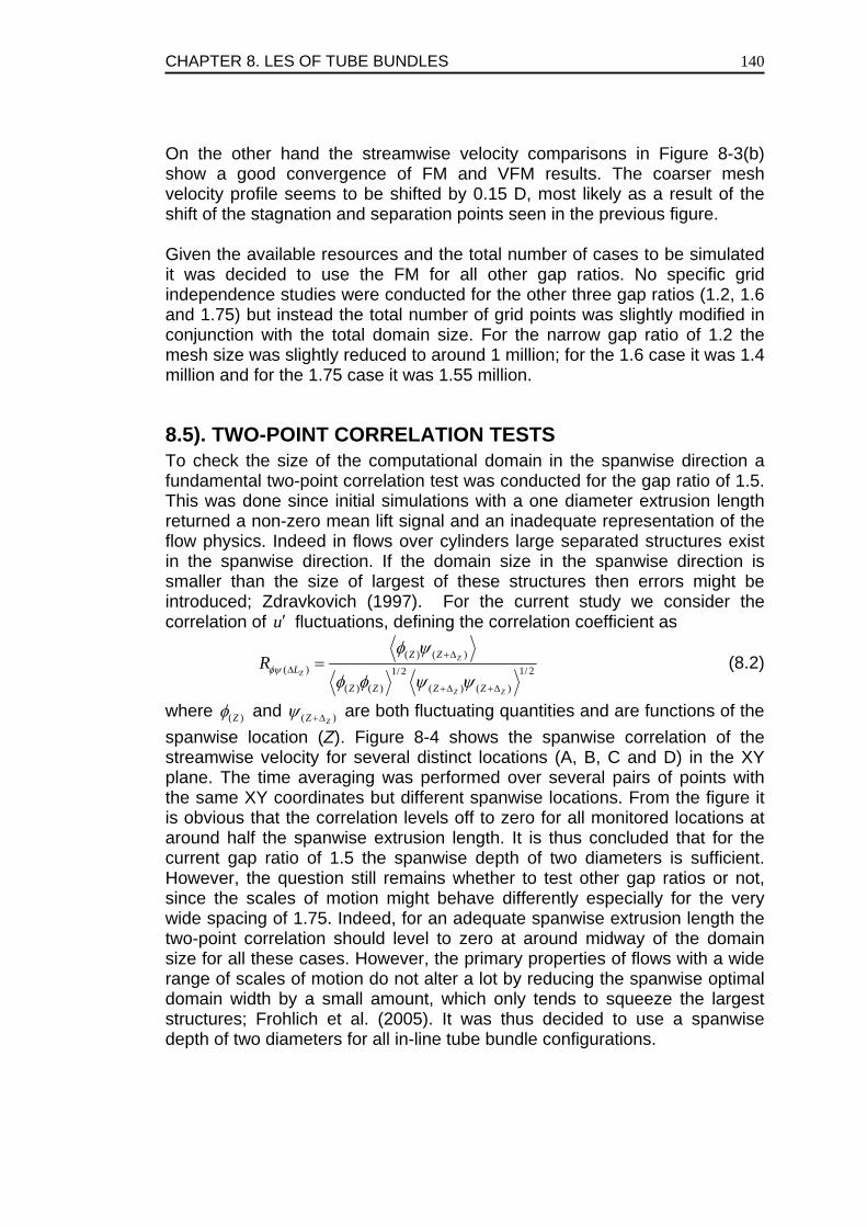
CHAPTER 8. LES OF TUBE BUNDLES
140
On the other hand the streamwise velocity comparisons in Figure 8-3(b) show a good convergence of FM and VFM results. The coarser mesh velocity profile seems to be shifted by 0.15 D, most likely as a result of the shift of the stagnation and separation points seen in the previous figure. Given the available resources and the total number of cases to be simulated it was decided to use the FM for all other gap ratios. No specific grid independence studies were conducted for the other three gap ratios (1.2, 1.6 and 1.75) but instead the total number of grid points was slightly modified in conjunction with the total domain size. For the narrow gap ratio of 1.2 the mesh size was slightly reduced to around 1 million; for the 1.6 case it was 1.4 million and for the 1.75 case it was 1.55 million.
8.5). TWO-POINT CORRELATION TESTS To check the size of the computational domain in the spanwise direction a fundamental two-point correlation test was conducted for the gap ratio of 1.5. This was done since initial simulations with a one diameter extrusion length returned a non-zero mean lift signal and an inadequate representation of the flow physics. Indeed in flows over cylinders large separated structures exist in the spanwise direction. If the domain size in the spanwise direction is smaller than the size of largest of these structures then errors might be introduced; Zdravkovich (1997). For the current study we consider the correlation of u′ fluctuations, defining the correlation coefficient as
( ) ( )( ) 1/ 21/ 2
( ) ( ) ( ) ( )
Z
Z
Z Z
Z ZL
Z Z Z Z
Rφψ
φ ψ
φ φ ψ ψ
+∆∆
+∆ +∆
= (8.2)
where ( )Zφ and ( )ZZψ +∆ are both fluctuating quantities and are functions of the spanwise location (Z). Figure 8-4 shows the spanwise correlation of the streamwise velocity for several distinct locations (A, B, C and D) in the XY plane. The time averaging was performed over several pairs of points with the same XY coordinates but different spanwise locations. From the figure it is obvious that the correlation levels off to zero for all monitored locations at around half the spanwise extrusion length. It is thus concluded that for the current gap ratio of 1.5 the spanwise depth of two diameters is sufficient. However, the question still remains whether to test other gap ratios or not, since the scales of motion might behave differently especially for the very wide spacing of 1.75. Indeed, for an adequate spanwise extrusion length the two-point correlation should level to zero at around midway of the domain size for all these cases. However, the primary properties of flows with a wide range of scales of motion do not alter a lot by reducing the spanwise optimal domain width by a small amount, which only tends to squeeze the largest structures; Frohlich et al. (2005). It was thus decided to use a spanwise depth of two diameters for all in-line tube bundle configurations.
CHAPTER 8. LES OF TUBE BUNDLES
141
8.6). RESULTS AND DISCUSSIONS In this section the flow physics, pressure distributions, velocity profiles, turbulence intensities, Strouhal numbers and lift and drag parameters will be discussed for all the cases.
8.6.1). FLOW PHYSICS The flow across square in-line tube bundles is inherently unstable and asymmetric for narrow gap ratios whereas it tends to become stable and symmetrical as the gap ratio is relaxed. Kim & Durbin (1988) observed that a bistable flow pattern exists which switches intermittently from being directed towards one cylinder to the other. Ishigai et al. (1973) report that the Reynolds number has little or no effect on this bistable flow pattern. In fact after preliminary simulations it was found that the flow behaves in a similar way even for fairly low Reynolds numbers (this is true when the flow is in the fully developed turbulent range). At lower Reynolds numbers (500-3,000) for a single row of cylinders Sumner et al. (1999) observed a similar asymmetrical flow behaviour for gap ratios between 1.2 and 2.2. Figure 8-5 shows the pseudo-average (2-D) mean velocity streamlines for the various gap ratios obtained from LES at a bulk gap Reynolds number of 45,000. It is seen from Figure 8-5(a) that for the gap ratio of 1.2 the flow is completely unidirectional and asymmetrical with much delayed separation taking place only at the top end of the cylinder surface resulting in a single tiny vortex behind the centre cylinder. It is as if the flow “preferred” to meander between the tubes in the diagonal rather than in the inline direction to avoid a series of sudden contractions and expansions which could entail more energy loss than the diagonal direction. One can also interpret this solution as a succession of Coanda effects, with the main stream staying attached to the curved wall as long as possible to avoid large (energy dissipating) separation and recirculation zones. It is interesting to note here that for this gap ratio of 1.2 one observes odd-odd12 or persistently asymmetric behaviour for all set of tubes; that is the flow in all gaps has the same asymmetry and the domain size could have been reduced to one fourth with periodic boundary condition. As the gap ratio is relaxed to 1.5 the flow physics changes. One now observes that the shear layer separates from the bottom of the cylinder surface as well resulting in two recirculation regions behind every cylinder. However, the flow is still asymmetrical with one recirculation bubble considerably larger than the other (see Figure 8-5(b), centre cylinder). One observes from Figure 8-5(b) that the flow is still showing persistently asymmetric behaviour with flow going up between all rows of cylinders.
12 Flow deflection to one side across a row of cylinders is termed as odd behavior. For the same sense of deflection across two set of rows of cylinders it is called odd-odd (persistently asymmetric). If an opposite sense of deflection exists then it is be termed as odd-even (alternating asymmetric).
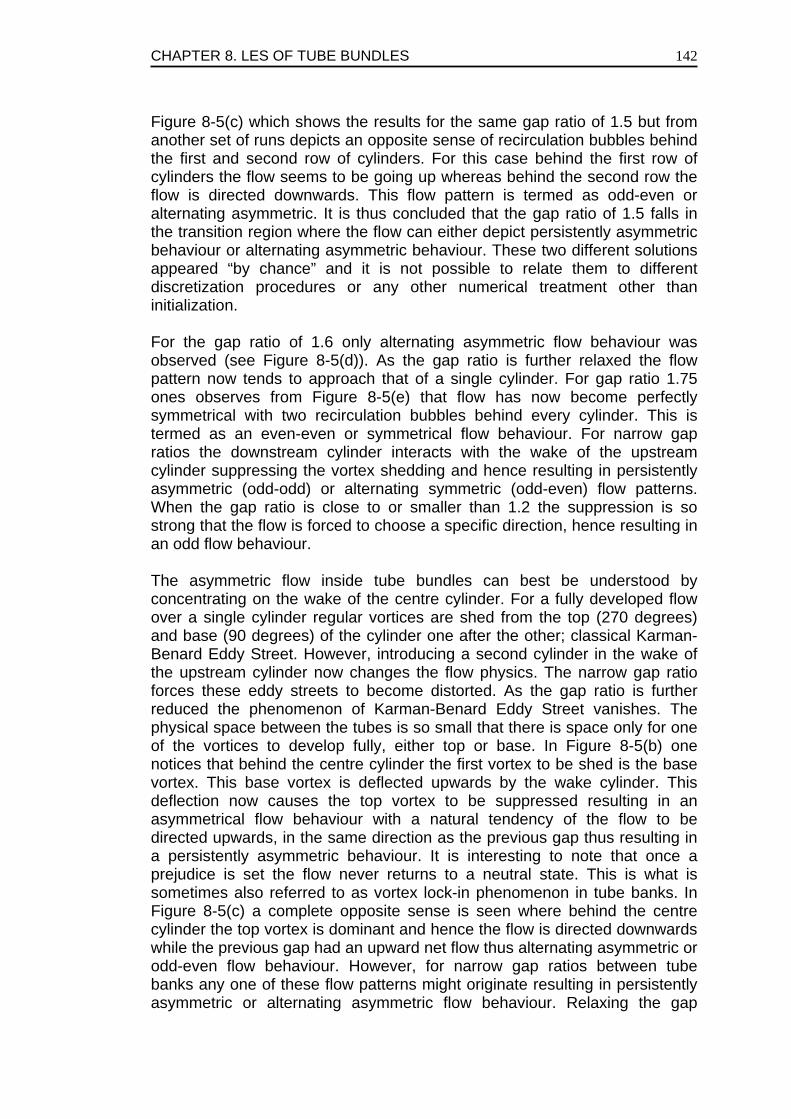
CHAPTER 8. LES OF TUBE BUNDLES
142
Figure 8-5(c) which shows the results for the same gap ratio of 1.5 but from another set of runs depicts an opposite sense of recirculation bubbles behind the first and second row of cylinders. For this case behind the first row of cylinders the flow seems to be going up whereas behind the second row the flow is directed downwards. This flow pattern is termed as odd-even or alternating asymmetric. It is thus concluded that the gap ratio of 1.5 falls in the transition region where the flow can either depict persistently asymmetric behaviour or alternating asymmetric behaviour. These two different solutions appeared “by chance” and it is not possible to relate them to different discretization procedures or any other numerical treatment other than initialization. For the gap ratio of 1.6 only alternating asymmetric flow behaviour was observed (see Figure 8-5(d)). As the gap ratio is further relaxed the flow pattern now tends to approach that of a single cylinder. For gap ratio 1.75 ones observes from Figure 8-5(e) that flow has now become perfectly symmetrical with two recirculation bubbles behind every cylinder. This is termed as an even-even or symmetrical flow behaviour. For narrow gap ratios the downstream cylinder interacts with the wake of the upstream cylinder suppressing the vortex shedding and hence resulting in persistently asymmetric (odd-odd) or alternating symmetric (odd-even) flow patterns. When the gap ratio is close to or smaller than 1.2 the suppression is so strong that the flow is forced to choose a specific direction, hence resulting in an odd flow behaviour. The asymmetric flow inside tube bundles can best be understood by concentrating on the wake of the centre cylinder. For a fully developed flow over a single cylinder regular vortices are shed from the top (270 degrees) and base (90 degrees) of the cylinder one after the other; classical Karman-Benard Eddy Street. However, introducing a second cylinder in the wake of the upstream cylinder now changes the flow physics. The narrow gap ratio forces these eddy streets to become distorted. As the gap ratio is further reduced the phenomenon of Karman-Benard Eddy Street vanishes. The physical space between the tubes is so small that there is space only for one of the vortices to develop fully, either top or base. In Figure 8-5(b) one notices that behind the centre cylinder the first vortex to be shed is the base vortex. This base vortex is deflected upwards by the wake cylinder. This deflection now causes the top vortex to be suppressed resulting in an asymmetrical flow behaviour with a natural tendency of the flow to be directed upwards, in the same direction as the previous gap thus resulting in a persistently asymmetric behaviour. It is interesting to note that once a prejudice is set the flow never returns to a neutral state. This is what is sometimes also referred to as vortex lock-in phenomenon in tube banks. In Figure 8-5(c) a complete opposite sense is seen where behind the centre cylinder the top vortex is dominant and hence the flow is directed downwards while the previous gap had an upward net flow thus alternating asymmetric or odd-even flow behaviour. However, for narrow gap ratios between tube banks any one of these flow patterns might originate resulting in persistently asymmetric or alternating asymmetric flow behaviour. Relaxing the gap
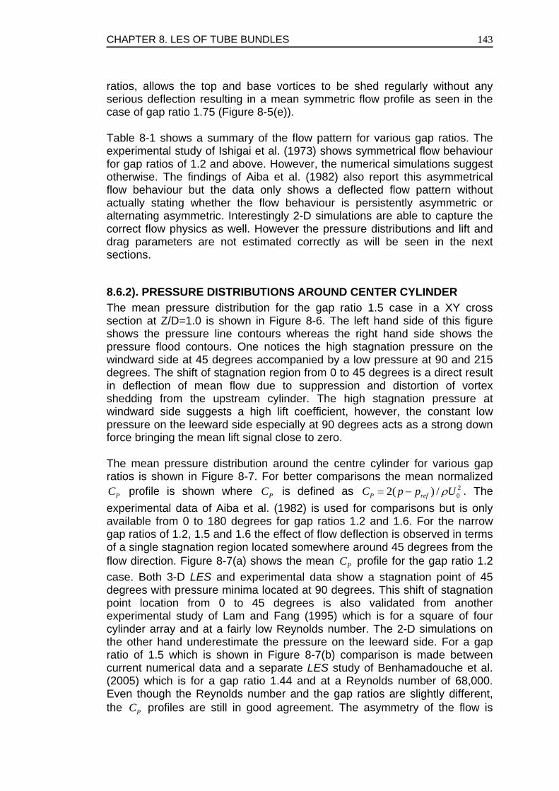
CHAPTER 8. LES OF TUBE BUNDLES
143
ratios, allows the top and base vortices to be shed regularly without any serious deflection resulting in a mean symmetric flow profile as seen in the case of gap ratio 1.75 (Figure 8-5(e)). Table 8-1 shows a summary of the flow pattern for various gap ratios. The experimental study of Ishigai et al. (1973) shows symmetrical flow behaviour for gap ratios of 1.2 and above. However, the numerical simulations suggest otherwise. The findings of Aiba et al. (1982) also report this asymmetrical flow behaviour but the data only shows a deflected flow pattern without actually stating whether the flow behaviour is persistently asymmetric or alternating asymmetric. Interestingly 2-D simulations are able to capture the correct flow physics as well. However the pressure distributions and lift and drag parameters are not estimated correctly as will be seen in the next sections.
8.6.2). PRESSURE DISTRIBUTIONS AROUND CENTER CYLINDER The mean pressure distribution for the gap ratio 1.5 case in a XY cross section at Z/D=1.0 is shown in Figure 8-6. The left hand side of this figure shows the pressure line contours whereas the right hand side shows the pressure flood contours. One notices the high stagnation pressure on the windward side at 45 degrees accompanied by a low pressure at 90 and 215 degrees. The shift of stagnation region from 0 to 45 degrees is a direct result in deflection of mean flow due to suppression and distortion of vortex shedding from the upstream cylinder. The high stagnation pressure at windward side suggests a high lift coefficient, however, the constant low pressure on the leeward side especially at 90 degrees acts as a strong down force bringing the mean lift signal close to zero. The mean pressure distribution around the centre cylinder for various gap ratios is shown in Figure 8-7. For better comparisons the mean normalized
PC profile is shown where PC is defined as 202( ) /P refC p p Uρ= − . The
experimental data of Aiba et al. (1982) is used for comparisons but is only available from 0 to 180 degrees for gap ratios 1.2 and 1.6. For the narrow gap ratios of 1.2, 1.5 and 1.6 the effect of flow deflection is observed in terms of a single stagnation region located somewhere around 45 degrees from the flow direction. Figure 8-7(a) shows the mean PC profile for the gap ratio 1.2 case. Both 3-D LES and experimental data show a stagnation point of 45 degrees with pressure minima located at 90 degrees. This shift of stagnation point location from 0 to 45 degrees is also validated from another experimental study of Lam and Fang (1995) which is for a square of four cylinder array and at a fairly low Reynolds number. The 2-D simulations on the other hand underestimate the pressure on the leeward side. For a gap ratio of 1.5 which is shown in Figure 8-7(b) comparison is made between current numerical data and a separate LES study of Benhamadouche et al. (2005) which is for a gap ratio 1.44 and at a Reynolds number of 68,000. Even though the Reynolds number and the gap ratios are slightly different, the PC profiles are still in good agreement. The asymmetry of the flow is
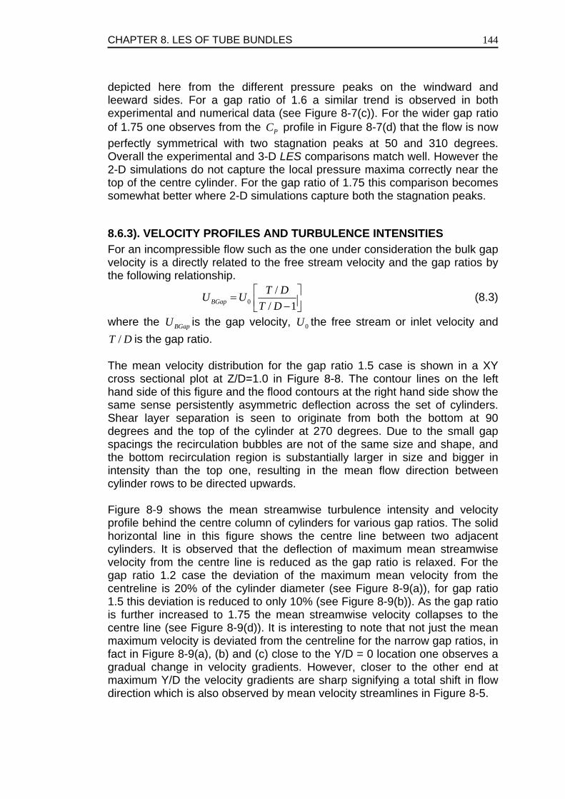
CHAPTER 8. LES OF TUBE BUNDLES
144
depicted here from the different pressure peaks on the windward and leeward sides. For a gap ratio of 1.6 a similar trend is observed in both experimental and numerical data (see Figure 8-7(c)). For the wider gap ratio of 1.75 one observes from the PC profile in Figure 8-7(d) that the flow is now perfectly symmetrical with two stagnation peaks at 50 and 310 degrees. Overall the experimental and 3-D LES comparisons match well. However the 2-D simulations do not capture the local pressure maxima correctly near the top of the centre cylinder. For the gap ratio of 1.75 this comparison becomes somewhat better where 2-D simulations capture both the stagnation peaks.
8.6.3). VELOCITY PROFILES AND TURBULENCE INTENSITIES For an incompressible flow such as the one under consideration the bulk gap velocity is a directly related to the free stream velocity and the gap ratios by the following relationship.
0/
/ 1BGapT DU U
T D⎡ ⎤= ⎢ ⎥−⎣ ⎦
(8.3)
where the BGapU is the gap velocity, 0U the free stream or inlet velocity and /T D is the gap ratio.
The mean velocity distribution for the gap ratio 1.5 case is shown in a XY cross sectional plot at Z/D=1.0 in Figure 8-8. The contour lines on the left hand side of this figure and the flood contours at the right hand side show the same sense persistently asymmetric deflection across the set of cylinders. Shear layer separation is seen to originate from both the bottom at 90 degrees and the top of the cylinder at 270 degrees. Due to the small gap spacings the recirculation bubbles are not of the same size and shape, and the bottom recirculation region is substantially larger in size and bigger in intensity than the top one, resulting in the mean flow direction between cylinder rows to be directed upwards. Figure 8-9 shows the mean streamwise turbulence intensity and velocity profile behind the centre column of cylinders for various gap ratios. The solid horizontal line in this figure shows the centre line between two adjacent cylinders. It is observed that the deflection of maximum mean streamwise velocity from the centre line is reduced as the gap ratio is relaxed. For the gap ratio 1.2 case the deviation of the maximum mean velocity from the centreline is 20% of the cylinder diameter (see Figure 8-9(a)), for gap ratio 1.5 this deviation is reduced to only 10% (see Figure 8-9(b)). As the gap ratio is further increased to 1.75 the mean streamwise velocity collapses to the centre line (see Figure 8-9(d)). It is interesting to note that not just the mean maximum velocity is deviated from the centreline for the narrow gap ratios, in fact in Figure 8-9(a), (b) and (c) close to the Y/D = 0 location one observes a gradual change in velocity gradients. However, closer to the other end at maximum Y/D the velocity gradients are sharp signifying a total shift in flow direction which is also observed by mean velocity streamlines in Figure 8-5.
CHAPTER 8. LES OF TUBE BUNDLES
145
One observes from Figure 8-9 that the mean streamwise turbulence intensity is directly related to the velocity gradients between cylinders. The regions of high velocity gradients show high turbulence intensity as can be expected. For the narrow gap ratio of 1.2 in Figure 8-9(a) one observes that the maximum streamwise turbulence intensity is around 80%. However, as the gap ratio is relaxed both the maximum mean streamwise velocity and the turbulence intensity decreases. For the gap ratio 1.5 case the maximum mean streamwise velocity is 3 whereas the corresponding maximum turbulence intensity is decreased to 60% which now shows four developing peaks (see Figure 8-9(b)). For the gap ratio 1.6 case in Figure 8-9(c), the experimental data of Aiba et al. (1982) shows a good comparison with the 3-D LES simulations. The maximum mean streamwise velocity in this case is around 2 and the maximum mean streamwise turbulence intensity is around 50%. For the gap ratio 1.75 the maximum turbulence intensity is further reduced. The maximum streamwise turbulence intensity now shows four symmetric peaks corresponding to two velocity peaks where the maximum intensity is now reduced to 35%. It is thus concluded that with increasing gap ratios both the mean streamwise velocity and turbulence intensity are decreased, similar to the findings of Aiba et al. (1982). To show the full three dimensionality of the flow Figure 8-10 is generated with multiple slices in the flow field for the intermediate gap ratio case of 1.5. Slices 1 and 2 are YZ cross sections at X=1.5 and 4.5 locations respectively. Slice 1 shows the contour lines and Slice 2 shows the flooded contours for normal v and spanwise w velocity. Interestingly one can notice the flow behaviour in the spanwise (Z) direction depicting strong asymmetry. Slices 3 and 4 are XY cross sections at Z/D=1.0 location for (0 3X≤ ≤ ) and (3 6X≤ ≥ ) respectively. These slices show the mean , ,u v w vector
plots (Slice 3) and the mean 2 2 2U u v w= + + contour floods (Slice 4)
depicting the two strong recirculation regions behind the leading cylinder.
8.6.4). LIFT AND DRAG FORCES The distorted vortex shedding and the full three-dimensionality of the flow causes highly fluctuating lift ( LC ) and drag ( DC ) forces, where the coefficients are computed using the projected area ( .ZA L D= ) of the cylinder and bulk gap velocity ( BGapU ). Lift and Drag coefficients are estimated numerically using the following formulas
2
2
2
2
XD
BGap
YL
BGap
FCU A
FCU A
ρ
ρ
=
= (8.4)
CHAPTER 8. LES OF TUBE BUNDLES
146
The streamwise ( XF ) and normal ( YF ) forces are the sum of the integrated wall pressure and the cylinder surface friction forces, where the contribution of the latter is found to be less than 5% of the total force and hence this friction component is commonly ignored while calculating the streamwise or drag coefficient; Kawamura et al. (1984). Table 8-2 shows the lift ( LC ), drag ( DC ) and their root mean square values ( LC ′ , DC ′ ) respectively for all gap ratios. Lack of experiential data makes it difficult to perform a complete comparison of numerical data. The experimental data of Pettigrew and Ko (1980) and Chen and Jendrzejczyk (1987) is used for comparison for gap ratios 1.5 and 1.75 cases respectively. The experimental data of Pettigrew and Ko (1980) is for an in-line configuration of a gap ratio of 1.47 and hence can be utilized for comparison with gap ratio 1.5 case. The mean pressure distribution of the centre cylinder showed a high stagnation pressure on the windward side close to 50 degrees for all narrow gap ratio cases (1.2, 1.5 and 1.6). However, this high pressure is being countered by a constant low pressure region on the leeward side especially at 90 degrees resulting in close to zero mean lift. Looking at the root mean square (r.m.s) values of lift and drag one observes that the r.m.s lift ( LC ′ ) coefficient is always larger than the r.m.s drag coefficient ( DC ′ ), as it should be according to Chen and Jendrzejczyk (1987). For gap ratio 1.5 case the r.m.s lift ( LC ′ ) and drag ( DC ′ ) coefficients fall within the experimental range of Pettigrew and Ko (1980). For the wider gap ratio of 1.75 the r.m.s drag coefficient ( DC ′ ) also falls within the experimental range of Chen and Jendrzejczyk (1987). However, the r.m.s lift ( LC ′ ) coefficient is slightly overestimated. For the 2-D cases the mean lift ( LC ) coefficients are also close to zero but mean drag ( DC ) coefficients are severely underestimated. The differences in mean pressure profiles in Figure 8-7 for the 2-D cases results in an over or under estimation of the r.m.s lift ( LC ′ ) and drag ( DC ′ ) coefficients. Note that the LES shows almost an order of magnitude increase in ( LC ′ ) between the two lower AR and the two higher ones. This is probably a sign that the strongly asymmetric mean vortex pair for low AR correspond to an absence of vortex shedding, while this shedding reappears for AR 1.75 and is present even at AR 1.6 A compilation of extensive experimental data by Weaver et al. (1986) leads to a best fit curve for the Strouhal number
1
2 1St
PD
=⎛ ⎞−⎜ ⎟⎝ ⎠
(8.5)
CHAPTER 8. LES OF TUBE BUNDLES
147
Figure 8-11 shows numerically obtained Strouhal numbers by Power Spectrum Density analysis of the lift signal for all cases. A comparison for numerically obtained Strouhal numbers with experimental values of Weaver et al. (1986) is also shown in Table 8-3. The numerically obtained Strouhal numbers straddle the experimental values showing that the vortex shedding detected in the shear layer with 3-D LES is realistic. For the gap ratio 1.5 case the Strouhal number based on gap velocity was also calculated since experimental data of Pettigrew and Ko (1980) was available. The 3-D LES value of 0.6512 compares quite well with the experimental range of 0.41-0.61. Overall the numerical Strouhal number comparison with available experimental data is quite well. However, it should be kept in mind that most of the experimental results are deduced from tube responses and not directly by forces measurements. Moreover, for in-line tube banks the vortex shedding phenomena is quite complex where multiple Strouhal numbers might exist; Weaver et al. (1986) and Fitzpatrick et al. (1986).
8.7). CONCLUSIONS Cross flow over 3-D square in-line tube bundles is investigated via Large Eddy Simulation for various gap ratios. Two-point correlation tests showed that one needs to take at least two diameters in the spanwise direction. 2-D simulations fail to capture the complete flow physics hence extensive 3-D LES were performed for all gap ratios. For the very narrow gap ratio of 1.2 a bistable strongly asymmetric solution is obtained with the mean flow highly deviated from the tube centrelines. For moderate gap ratios of 1.5 and 1.6 the flow deviation is not so strong but still an asymmetric solution is obtained. The vortices shed for these cases are highly distorted due to the blockage effect from downstream cylinders thus resulting in one large and one small vortex in the mean velocity filed. For narrow gap ratios of 1.2, 1.5 and 1.6 the stagnation point is well off the symmetry line and the top and bottom shear layer separation points are different from each other resulting in persistently asymmetric or alternating asymmetric flow pattern. For the wider gap ratio of 1.75 the flow is found to be perfectly symmetrical owing to larger tube spacing and smaller blockage effects. In this case two stagnation points are observed at 50 and 310 degrees on the centre cylinder. For this gap ratio the top and bottom shear layer separation points are the same thus leading to two symmetrical but mirrored vortices on the leeward side of the centre cylinder. Finally the length of the separation bubbles is also the same. Mean lift and drag coefficients and their root mean square values are predicted quite well for all the cases by 3-D LES. The r.m.s value of the lift coefficient was seen to increase by an order of magnitude between the lower and higher gap ratio. Strouhal numbers for all these cases are obtained by power density spectrum analysis. Partial experimental data is available for velocity, turbulence intensity, and pressure. In all cases where comparison is possible good agreement with this experimental data was found, which gives confidence in the use of LES for refined investigations of this type of flow.

CHAPTER 8. LES OF TUBE BUNDLES
148
For the next part of current study tests of Reynolds Averaged Navier Stokes (RANS) models, namely k ε− , RNG k ε− , MSST and SSG models, are conducted for the moderate gap ratio of 1.5. Successful testing of these models would enable economical parametric studies, eventually leading to design optimisation.
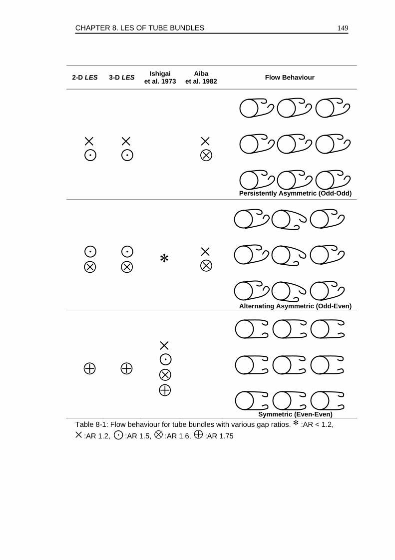
CHAPTER 8. LES OF TUBE BUNDLES
149
2-D LES 3-D LES Ishigai et al. 1973
Aiba et al. 1982 Flow Behaviour
×
×
×
⊗
Persistently Asymmetric (Odd-Odd)
⊗
⊗ ∗
×
⊗
Alternating Asymmetric (Odd-Even)
⊕ ⊕
×
⊗
⊕
Symmetric (Even-Even) Table 8-1: Flow behaviour for tube bundles with various gap ratios. ∗ :AR < 1.2, ×:AR 1.2, :AR 1.5, ⊗ :AR 1.6, ⊕ :AR 1.75
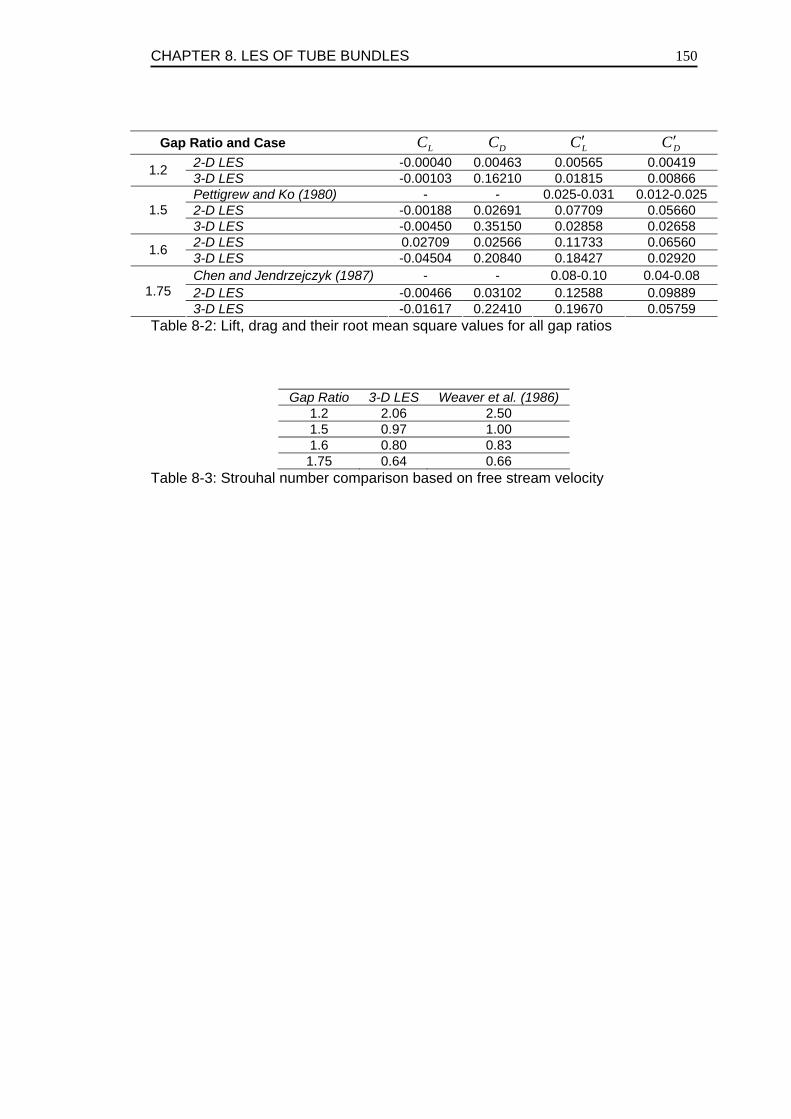
CHAPTER 8. LES OF TUBE BUNDLES
150
Gap Ratio and Case LC DC LC ′ DC ′
2-D LES -0.00040 0.00463 0.00565 0.00419 1.2 3-D LES -0.00103 0.16210 0.01815 0.00866 Pettigrew and Ko (1980) - - 0.025-0.031 0.012-0.025 2-D LES -0.00188 0.02691 0.07709 0.05660 1.5 3-D LES -0.00450 0.35150 0.02858 0.02658 2-D LES 0.02709 0.02566 0.11733 0.06560 1.6 3-D LES -0.04504 0.20840 0.18427 0.02920 Chen and Jendrzejczyk (1987) - - 0.08-0.10 0.04-0.08 2-D LES -0.00466 0.03102 0.12588 0.09889 1.75 3-D LES -0.01617 0.22410 0.19670 0.05759
Table 8-2: Lift, drag and their root mean square values for all gap ratios
Gap Ratio 3-D LES Weaver et al. (1986) 1.2 2.06 2.50 1.5 0.97 1.00 1.6 0.80 0.83 1.75 0.64 0.66
Table 8-3: Strouhal number comparison based on free stream velocity
CHAPTER 8. LES OF TUBE BUNDLES
151
Figure 8-1: Geometry of in-line tube bundle configuration
CHAPTER 8. LES OF TUBE BUNDLES 152
(a)
(b)
(c)
Figure 8-2: Cross-sectional view of the grid in XY (Z=3) and YZ (X=3) plane. (a):
Coarse mesh (CM) 0.69 million cells, (b): Fine mesh (FM) 1.3 million cells, (c) Very
fine mesh (VFM) 2.4 million cells
CHAPTER 8. LES OF TUBE BUNDLES
153
(a)
(b)
Figure 8-3: Comparison of solution obtained with various grids, CM, FM and VFM for gap ratio 1.5. (a) CP along central cylinder, (b) streamwise velocity at X/D = 2.25
CHAPTER 8. LES OF TUBE BUNDLES
154
Figure 8-4: Spanwise correlation of streamwise velocity obtained with LZ=2D, at different points in the flow domain for gap ratio 1.5. A: (1.5, 1.5), B: (3.0, 4.5), C: (4.5, 3.0), D: (4.75, 0.85)
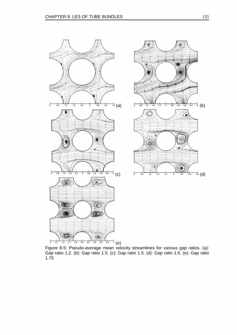
CHAPTER 8. LES OF TUBE BUNDLES
155
(a) (b)
(c) (d)
(e)
Figure 8-5: Pseudo-average mean velocity streamlines for various gap ratios. (a): Gap ratio 1.2. (b): Gap ratio 1.5. (c): Gap ratio 1.5. (d): Gap ratio 1.6. (e): Gap ratio 1.75
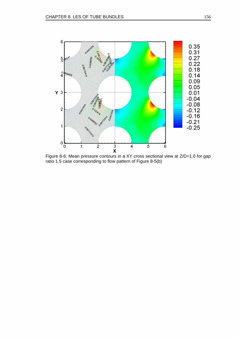
CHAPTER 8. LES OF TUBE BUNDLES
156
Figure 8-6: Mean pressure contours in a XY cross sectional view at Z/D=1.0 for gap ratio 1.5 case corresponding to flow pattern of Figure 8-5(b)
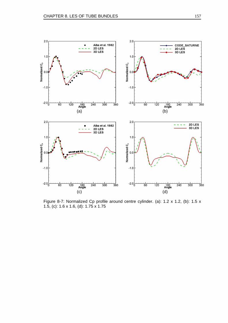
CHAPTER 8. LES OF TUBE BUNDLES
157
(a) (b)
(c) (d)
Figure 8-7: Normalized Cp profile around centre cylinder. (a): 1.2 x 1.2, (b): 1.5 x 1.5, (c): 1.6 x 1.6, (d): 1.75 x 1.75
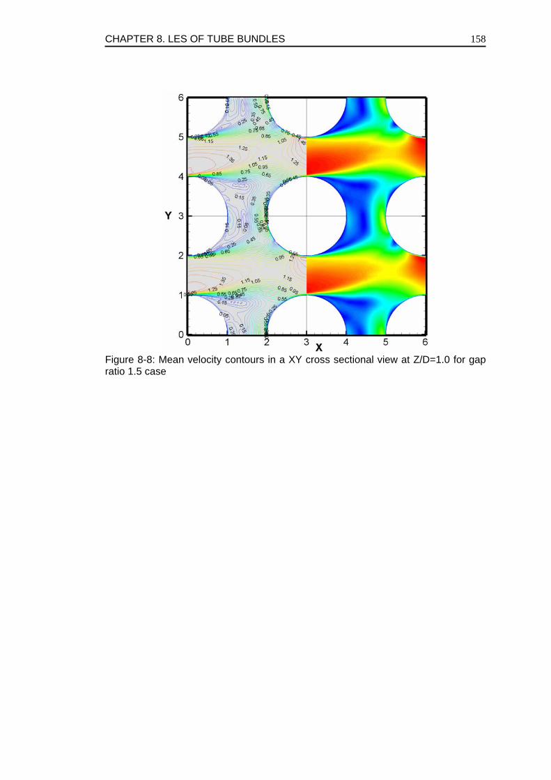
CHAPTER 8. LES OF TUBE BUNDLES
158
Figure 8-8: Mean velocity contours in a XY cross sectional view at Z/D=1.0 for gap ratio 1.5 case
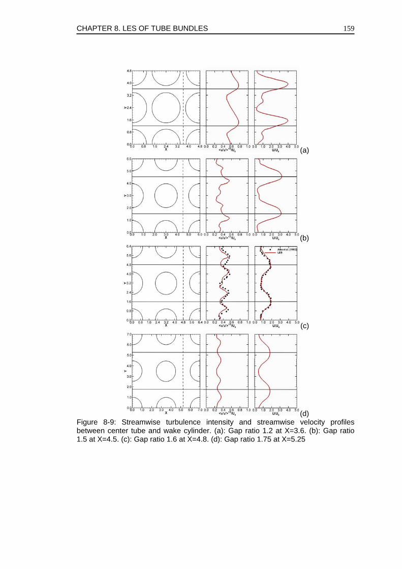
CHAPTER 8. LES OF TUBE BUNDLES
159
(a)
(b)
(c)
(d) Figure 8-9: Streamwise turbulence intensity and streamwise velocity profiles between center tube and wake cylinder. (a): Gap ratio 1.2 at X=3.6. (b): Gap ratio 1.5 at X=4.5. (c): Gap ratio 1.6 at X=4.8. (d): Gap ratio 1.75 at X=5.25
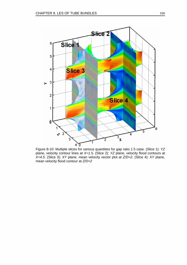
CHAPTER 8. LES OF TUBE BUNDLES
160
Figure 8-10: Multiple slices for various quantities for gap ratio 1.5 case. (Slice 1): YZ plane, velocity contour lines at X=1.5. (Slice 2): YZ plane, velocity flood contours at X=4.5. (Slice 3): XY plane, mean velocity vector plot at Z/D=2. (Slice 4): XY plane, mean velocity flood contour at Z/D=2
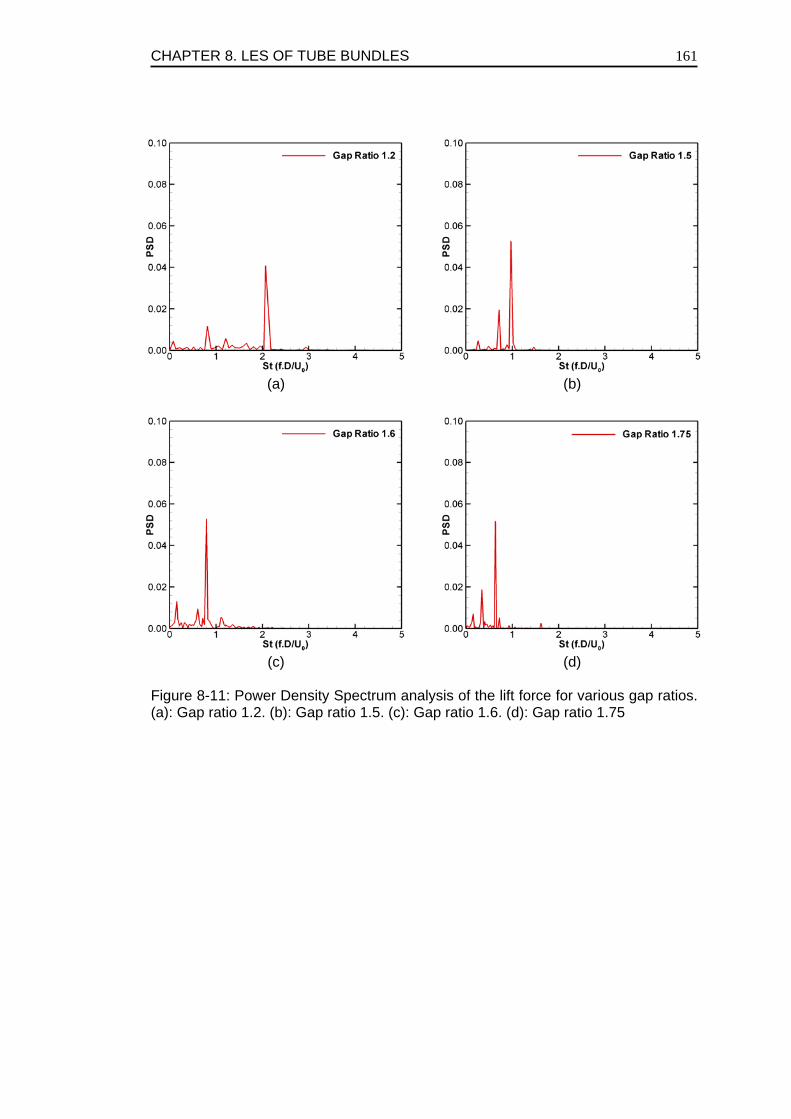
CHAPTER 8. LES OF TUBE BUNDLES
161
(a) (b)
(c) (d)
Figure 8-11: Power Density Spectrum analysis of the lift force for various gap ratios. (a): Gap ratio 1.2. (b): Gap ratio 1.5. (c): Gap ratio 1.6. (d): Gap ratio 1.75
CHAPTER 8. LES OF TUBE BUNDLES
162
BIBLIOGRAPHY Aiba, S., Tsuchida, H., Ota, T. 1982. Heat Transfer around Tubes in In-line Tube Banks. Bull. JSME, 25, 919-926. Benhamadouche, S., Laurence, D., 2003. LES, coarse LES, and transient RANS comparisons on the flow across tube bundle. Int. J. Heat Fluid Flow. 4, 470-479. Benhamadouche, S., Laurence, D., Jarrin, N., Afgan, I., Moulinec, C. 2005. Large Eddy Simulation of Flow Across In-line Tube Bundles, 11th International Topical Meeting on Nuclear Reactor Thermal-Hydraulics (NURETH-11), Popes’ Palace Conference Centre, Avignon, France. Paper: 405. Boris, J.P., Grinstein, F.F., Oran, E.S., Kolbe, R.L. 1992. New Insights into LES. Fluid Dyn. Res. 10, 199-228. Bouris, D., Bergeles, G. 1999. Two dimensional Time Dependent Simulation of the Subcritical Flow in a Staggered Tube Bundle using a Subgrid-scale Model. Int. J. Heat Fluid Flow. 20(2), 105-114. Bouris, D., Papadakis, G., Bergeles, G. 2001. Numerical Evaluation of Alternate Tube Configurations for Particle Deposition Rate in Heat Exchanger Tube Bundles. Int. J. Heat Fluid Flow. 22(5), 525-536. Breuer, M., Rodi, W. 1994. LES of Turbulent Flow through a Straight Square Duct and 1800 End. Voke, P. et al. (Eds), Direct and LES I. Kluwer Academic Publishers, Dordrecht. 273-285. Celik, I. B., Cehreli, Z. N., Yavuz, I. 2005. Index of resolution quality for Large Eddy Simulations. J. Fluids Eng. 127, 949-958. Chen, S. S. 1987. Flow-Induced Vibration of Circular Cylindrical Structures. Hemisphere publishing corporation. Chen, S.S., Jendrzejczyk, J.A. 1987. Fluid Excitation Forces Acting on a Square Tube Array. JSME Transactions Vol 109, 415-423. Ferziger, J.H., Peric, M. 2002. Computational Methods for Fluid Dynamics. Springer, third edition. Fitz-Hugh, J.S. 1973. Flow Induced Vibration in Heat Exchangers. Proc. Int. Sym. on Vibration Problems in Industry, Keswick, UK, Paper No. 427; in Flow induced vibration of circular cylinder structures by Chen, S. S.
CHAPTER 8. LES OF TUBE BUNDLES
163
Frohlich, J. Rodi, W. 2002. Introduction to Large Eddy Simulation of Turbulent Flows. Closure strategies for turbulent and transitional flows by B. Launder and N. Sandham, Cambridge University press. 267-298. Hassan, Y., Ibrahim, W. 1997. Turbulence Prediction in Two-Dimensional Tube Bundle Flows using Large Eddy Simulation, Nuclear Technology 119, 11-28. Ishigai, S., Nishikawa, E., Yagi, E. 1973. Structures of Gas Flow and Vibration in Tube Banks with Tube Axes Normal to Flow. Inst. Sym. on Marine Engineering, Tokyo. PP. 1-5-23 to 1-5-33; in Flow induced vibration of circular cylinder structures by Chen, S. S. Kawamura, T., Hiwada, M., Hibino, T., Mabuchi, I., Kamuda, M., 1984. Flow around a finite circular cylinder on a flat plate. Bull. JSME 27 (232), 2142-2151. Kim, H.J., Durbin, P.A. 1988. Investigation of the Flow between a Pair of Circular Cylinders in the Flopping Regime. J. Fluid Mech. 196. 431-448. Kravchenko, A.G., Moin, P. 1997. On the Effects of Numerical Errors in Large Eddy Simulation of Turbulent Flows. J. Comp. Phys. 131. 310-322. Lam, K., Fang, X. 1995. The Effect of Interference of Four Equispaced Cylinders in Cross Flow on Pressure and Force Coefficients. J. Fluids Struct. 9. 195-214. Meyer, K.E. 1994. Experimental and Numerical Investigation of Turbulent Flow and Heat Transfer in Staggered Tube Bundles. Ph. D. Thesis, AFM 94-03, Tech. Univ. of Denmark. Moulinec, C., Hunt, J. C. R., Nieuwstadt, F. T. M. 2004. Disappearing Wakes and Dispersion in Numerically Simulated Flows through Tube Bundles. Flow, Turb. Comb. 73: 95-116. Peric, M. 2004. Flow Simulation Using Control Volumes of Arbitrary Polyhedral Shape, ERCOFTAC bulletin No. 62, Page 25-29. Pettigrew, M.J., Ko, P.L. 1980. A Comprehensive Approach to avoid Vibration and Fretting in Shell-and-Tube Heat Exchangers. Flow induced vibration of power plant components, PVP-41, ASME publications, pp. 1-18. Price, S.J., Paidoussis, M.P. 1997. An Improved Mathematical Model for the Stability of Cylinder Flows Subject to Cross-Flow, J. Sound Vibrat. 97(4), 615-640. Rollet-Miet, P., Laurence, D., Ferziger, J. 1999. LES and RANS of Turbulent Flow in Tube Bundles, Int. J. Heat Fluid Flow. 20, 241-254.
CHAPTER 8. LES OF TUBE BUNDLES
164
Sebag, S., Maupu, V., Laurence, D. 1991. Non-Orthogonal Calculation Procedures using Second Moment Closures, TSF 8. Sumner, D., Wong, S.S.T., Price, S.J., Paidoussis, M.P. 1999. Fluid Behaviour of Side by Side Circular Cylinders in Steady Cross-Flow. J. Fluids Struct. 13. 309-338. Weaver, D.S., Fitzpatrick, J.A., Elkashlan, H. 1986. Strouhal Numbers for Heat Exchanger Tube Arrays in Cross Flow. J. of Press. Vess. Tech. 109, 219-223. Zdravkovich, M.M., Sing, S., Nuttall, J.A., Causon, D.M. 1976. Flow Induced Vibration in Staggered Tube Banks. Sixth Thermodynamics and fluid mechanics convention, University of Durham, April 1976; in Flow induced vibration of circular cylinder structures by Chen, S. S. Zdravkovich, M. M. 1997. Flow Around Circular Cylinders, Volume 2. Oxford University Press.
CHAPTER 9. URANS OF TUBE BUNDLES
165
Chapter 9 . SIMULATION OF FLOW IN TUBE BUNDLES BY URANS
9.1). INTRODUCTION In the previous chapter we showed the results of Large Eddy Simulations (LES) for various gap ratios for cross flow over in-line tube bundles. However, limitations in computational resources and project deadlines can sometimes serve as serious industrial constraints. It is thus understandable to test some Unsteady Reynolds Averaged Navier Stokes (URANS) models on one of the tube bundle configurations. For the current simulations the intermediate gap ratio of 1.5 was thus selected. Various 2-D and 3-D URANS models were tested for this configuration and the URANS data was then compared to the 3-D LES data which served as a benchmark. This LES data has already been exhaustively tested and compared to experimental data in the previous chapter. The in-depth comparison will comprise of pressure distributions, velocity profiles, Reynolds stresses, turbulence kinetic energy and lift and drag parameters. Reynolds Averaged Navier Stokes (RANS) models when applied to staggered tube bundles have so far not produced any reliable results as was cited previously; Rollet-Miet et al. (1999), Sebag et al. (1991), Meyer (1994), and Bouris and Bergeles (1999). It is concluded that even advanced TRANS models such as non-linear, realizable and RNG types of k ε− models severely underestimate the high turbulent kinetic energy levels observed in densely packed staggered tube bundles. Paradoxically there are some literature citations in which the standard k ε− model returns reasonable predictions of mean velocities and global level of turbulent kinetic energy. This has been reported to be due to erroneous overproduction of kinetic energy on the impinging side of the tubes which artificially raises the overall turbulence intensity but the locations of the maximum and minimum values are still erroneous; Benhamadouche and Laurence (2003). According to Hanjalic and Kenjeres (2006) in general the RANS models have serious limitations such as lack of generality in the sense that they cannot account for various turbulence scales that characterize the turbulence dynamics. In flows with dominant large eddy structures these issues become very important and can lead to major shortcomings in the simulated results. However,
CHAPTER 9. URANS OF TUBE BUNDLES
166
Benhamadouche and Laurence (2003) found fairly good results with 3D URANS based on a Reynolds Stress model for the staggered tube bundle. In the context of the current research this justifies the testing of various URANS models for inline tube bundles especially to address the aforementioned issues.
9.2). CASE DESCRIPTION AND NUMERICS The tube bundle configuration with a gap ratio of 1.5 is numerically simulated using various URANS models. 2-D and 3-D ensemble averaged Navier-Stokes equations on unstructured grids are solved using a finite volume approach. The URANS models tested are k ε− , renormalization group theory k ε− , Menter’s Shear Stress Transport (MSST) and the Speziale Sarkar Gatski (SSG) Reynolds stress model. These models have already been discussed in detail in earlier parts of the thesis and hence shall not be repeated. However, as a quick flashback, the standard k ε− and SSG models are both high Reynolds number models whereas RNG k ε− and MSST models are low Reynolds number models. The differences in model constants and governing equations lead to the use of different grid resolutions for the low and high Reynolds number models with a corresponding adjustment in the time stepping for the transient cases. However, these grid-related differences shall be discussed in the next section. In incompressible URANS the usual RANS equations are employed but with the transient (unsteady) term retained. The ensemble averaged transient RANS equations are then presented as
21i j i ji i
j i j j j
U U u uU UP vt x x x x xρ
′′ ′′∂ ∂∂ ∂∂+ = − + −
∂ ∂ ∂ ∂ ∂ ∂ (9.1)
Where iu′′are the modelled turbulent fluctuations. Just like LES even though the approach is transient or unsteady we are still interested in time averaged mean flow quantities, thus For URANS the time averaging approach is employed which is somewhat similar to LES
where U U u U U u
U U u u
′′ ′= + = +
′ ′′= + + (9.2)
Where U is the instantaneous quantity, U the time averaged quantity, u′ the resolved fluctuation and u′′ the modelled turbulent fluctuation. This basic approach has been implemented for the simulation of all URANS cases. Once the flow has been fully developed the statistics collection is initiated just like LES and a modelled part is added into the averaging terms to account for modelled fluctuations. This is done via additional user coding which can be found in the appendix of the thesis.
CHAPTER 9. URANS OF TUBE BUNDLES
167
The model dimensions and boundary conditions for the URANS cases are kept the same as in the LES case; 3 by 3 tubes with periodicity in all directions and a spanwise homogeneous extrusion length of 2 diameters (see the two point correlation tests in Chapter 8). The Reynolds number based on bulk gap velocity and cylinder diameter is 45,000 and the gap ratio is fixed at 1.5. To obtain the desired bulk velocity a self-correcting mean pressure gradient is specified at every time step which was done by adding a source term to the momentum equation, which is also explained in detail in the previous chapter. For all the URANS cases the total simulation has been allowed to run for approximately 17 complete flow passes and the averaging of statistics has been done over the last 12 passes. Spatial discretization for the URANS study is now 2nd order upwinding and time discretization by the 2nd order accurate TTLM scheme described in Ferziger and Peric (2002). Two different meshes were created for the URANS simulations; a coarse mesh for the high Reynolds number ( k ε− and SSG) models and a finer mesh for the low Reynolds number (RNG k ε− and MSST) models. The finer mesh was made in conjunction to the fact that the flow has to be resolved near to the wall which is an intrinsic requirement for the MSST model. Grid generation was done using a constructive geometric modelling approach. Two matching blocks were first generated with a non-conforming interface and were then copied 32 times using symmetries to get the final 2D grid. It is important to note that this ensures a fully symmetric grid as the flow solution will later be seen to be non-symmetric. Once this 2-D grid was obtained it was then extruded in the spanwise direction to get a 3-D grid. Figure 9-1 shows the front view of the 2-D grids for various URANS models. The size of the grids for both 2-D and 3-D simulations along with corresponding Y+ are given in Table 9-1.
9.3). RESULTS AND DISCUSSIONS
9.3.1). FLOW PHYSICS Cross flow inside narrow in-line tube bundles is inherently unstable and asymmetric showing even-odd or odd-odd flow pattern. For narrow gap ratios (1.2 / 1.6P D< < ) the cylinders are subjected to strong proximity interference. This interference suppresses the regular vortex shedding form the upstream cylinders causing distorted and highly deflected vortex shedding. Once a prejudice or bias is set in the direction of vortex shedding the flow hardly or never returns to a natural state, showing a time averaged asymmetrical flow behaviour. Depending upon the direction of the flow deflection the flow behaviour is termed as even-odd (up-down/down-up) or odd-odd (up-up/down-down). This peculiar flow behaviour was observed and discussed in detail in the preceding chapters. As the gap ratio is increased regular vortex shedding is facilitated making the mean flow less and less deflected toward one side. For a gap ratio of 1.75 this flow deflection vanishes and a regular symmetrical mean flow is observed. The current case with a gap ratio of 1.5 is chosen so as to
CHAPTER 9. URANS OF TUBE BUNDLES
168
investigate the degree of accuracy to which the URANS simulations capture this peculiar flow behaviour. Both 2-D and 3-D URANS results will be comprehensively compared to LES data for the same configuration. The mean normalized PC profile for the centre cylinder is shown in Figure 9-2. The 2-D URANS results are compared to the 3-D LES STAR-V4 in Figure 9-2(a) whereas the 3-D URANS results are shown in Figure 9-2(b). The angle measurement which is shown in Figure 9-2(a) is counter clockwise and starts from the inlet free stream direction that is from left to right. Interestingly all the 2-D RANS capture the asymmetry in the flow behaviour. However, the negative pressure is severely over estimated by all the models at around 90 degrees. The local pressure maxima located at 315 degrees is also over-estimated by all the 2-D RANS models. When looking at 3-D URANS results in Figure 9-2(b) one observes that the LES STAR-V4 and LES Code Saturne are in close agreement whereas the standard k ε− and the RNG k ε− models still over predict the negative pressure. In fact there seems to be little or no difference in the 2-D and 3-D profiles for these two models. On the other hand the 3-D MSST and SSG models are now close to LES results. However they still seem to be slightly over-predicting the local pressure maxima at 315 degrees. Over-prediction in the location of the stagnation point is also quite apparent in the 2-D RANS results where all the RANS models predict the value to be close to around 60 degrees. The standard k ε− and the RNG k ε− models in 3-D cases still over predict this stagnation point location. The 3-D MSST model slightly over predicts this value to around 55 degrees, whereas the SSG model is closer to the two LES (45-50 degrees). The Pseudo-average mean velocity streamlines in central XY plane for all 2-D RANS models along with 3-D LES are shown in Figure 9-3. One notices from Figure 9-3(a)-(d) that the 2-D models (standard k ε− , RNG k ε− , MSST and SSG) fail to capture the shear layer separation from the top of the cylinder; the only visible vortex is the one near the base. In Figure 9-3(c) and (d), however, one notices the existence of a secondary vortex just before the central cylinder at around 330 degrees. This secondary vortex, although captured, is still by far over estimated by the two RANS models compared to the one depicted by the 3-D LES (Figure 9-3(e)). The flow asymmetry is still clearly captured by all 2-D RANS models which is a good indication. Figure 9-4 shows the streamlines for 3-D simulations. These results seem to be significantly promising especially for the MSST and SSG models. In 3-D one notices from Figure 9-4(c) and (d) that the MSST and SSG models capture both the top and bottom shear layer separations showing the existence of both primary and secondary vortices. For the 3-D MSST and SSG cases the third vortex at 330 degrees just before the central cylinder is also captured, however it is overestimated for the MSST model and underestimated by the SSG model (see Figure 9-4(c) and (d)). For the standard k ε− and RNG k ε− models this vortex is not captured at all (see Figure 9-4(a) and (b)). Thus the PC profiles for these two cases in Figure 9-2(b) remain mostly
CHAPTER 9. URANS OF TUBE BUNDLES
169
unchanged except at 225 degrees where the standard k ε− model is slightly closer to LES than RNG k ε− model. Figure 9-5 shows the mean pressure distribution in a XY cross section at Z/D=1.0 for various 3-D URANS models. The left hand side of these figures shows the mean pressure contour lines whereas right side shows the isobars. For an accurate comparison all the plots are drawn on a same scale of -0.25 to 0.35. One notices from these figures that k ε− and RNG k ε− models severely over predict the negative pressure both at 90 degrees and at 270 degrees (see Figure 9-5(a) and (b)). The balance of these two severe negative pressures on opposite sides leads to a close to zero mean lift for both these models as will be seen in Table 9-2 later. On the other hand the MSST model and the SSG models shown in Figure 9-5(c) and (d) respectively are in closer agreement with the LES pressure plot in Figure 9-5(e). The MSST model however, still shows a slight over prediction of mean pressure around 315 degrees. This effect of high pressure is also noticed in the mean velocity streamlines in Figure 9-4(c) which showed an over prediction in the size of a recirculation bubble near 315 degrees. In terms of flow physics not much difference was observed in results between 2-D and 3-D k ε− and RNG k ε− models. This was initially noticed in Figure 9-2 in which the pressure profile around the central cylinder was shown. Figure 9-6 shows the sectional view of the mean pressure profile on the cylinder surface along with a cross section in YZ plane for all the 3-D URANS models. One notices that for k ε− and RNG k ε− models the central cylinder and the cross sectional plane do not show any pressure variation. Thus for k ε− and RNG k ε− models the 3-D runs showed no edge over their 2-D counterparts. However, for the MSST and SSG models (Figure 9-6(c) and (d)) both the cylinder surface and the cross sectional plane show a pressure variation along the spanwise (Z) direction quite similar to what was observed in the earlier LES study.
9.3.2). VELOCITY PROFILES AND TURBULENCE INTENSITIES For the 3-D URANS cases the mean velocity along a vertical line in XY plane at X=4.5 and Z=2.0 is shown in Figure 9-7(a). One notices that both k ε− and RNG k ε− models under predict the velocity. On the other hand the total turbulence kinetic energy along the same line is substantially under predicted by all URANS models (see Figure 9-7(b)). Ironically, the prediction of the k ε− model is closest to the LES profile which is considered as a coincidence since the model does not depict the true 4 peaks. The MSST and SSG model’s predictions here are far better than the other URANS models since they tend to capture all the local peaks in the turbulence profile. However, the MSST model substantially under predicts the turbulence intensity which is almost 50% of what the LES suggests. A thorough breakdown of Reynolds stresses is shown in Figure 9-8 for the LES and SSG models. The figure shows the time averaged u u′ ′< > , v v′ ′< > , w w′ ′< > and
u v′ ′< > profiles along the same line. One notices from this figure that the peaks in the streamwise and normal Reynolds stresses ( u u′ ′< > , v v′ ′< >
CHAPTER 9. URANS OF TUBE BUNDLES
170
respectively) are quite decently captured by the SSG model. Here the biggest discrepancy is in the spanwise component which is 40% less in magnitude than the LES prediction. Perhaps a spanwise increase in grid resolution might improve this situation to some extent.
9.3.3). LIFT AND DRAG FORCES As already explained in the last chapter the lift and drag coefficients are computed using the projected area of the central cylinder and the bulk gap velocity. The streamwise ( XF ) and normal ( YF ) forces are the sum of the integrated wall pressure and the cylinder surface friction forces. Table 9-2 shows the lift ( LC ), drag ( DC ) and their root mean square values ( LC ′ , DC ′ ) respectively for all 2-D and 3-D simulations. The experimental data of Pettigrew and Ko (1980) which is for a gap ratio 1.47 is used for comparison. The LES results of Code Saturne are also shown for a similar configuration (P/D=1.44) in this table. It is observed that all 2-D URANS models predict unrealistic lift and drag coefficients. However, for the 3-D cases, the results seem to be somewhat better. The k ε− and RNG k ε− models which hugely over predicted the negative pressures on the cylinder surface still result in close to a zero mean lift value. This is believed to be by chance that the over prediction on both bottom and top of the cylinder balance each other resulting in a net zero value. As a whole all the 3-D URANS models depict a mean zero lift value. However the mean drag is still substantially under-predicted by all the models. On the other hand the r.m.s lift and drag values for MSST and SSG models are still quite acceptable and lie within the experimental range of Pettigrew and Ko (1980) and are quite close to LES STAR-V4 results. Unfortunately the LES Code Saturne r.m.s lift and drag values are quite higher than all other simulations and experimental data which needs to be closely examined. Perhaps the insufficient grid resolution especially in the spanwise direction for LES Saturne runs is the problem. The resolution which is only 30 cells in spanwise direction should have been increased to get smaller z+∆ value.
9.4). CONCLUSIONS The cross flow over 3-D square in-line tube bundle of gap ratio 1.5 is investigated via different 2-D and 3-D URANS models and the results were compared to an LES study for the same configuration. The complex flow for this configuration has already been shown to be asymmetric in nature with a high deflection in the mean flow direction. It is seen that the 2-D URANS results tend to capture the basic asymmetry of the flow although lift and drag values are totally unrealistic. Moreover the pressure predictions on the surface of the cylinders are also under or over-estimated by all 2-D RANS models. 3-D URANS simulations on the other hand seem to produce better results, at least the MSST and SSG models. For the k ε− and RNG k ε− models no improvement in results was
CHAPTER 9. URANS OF TUBE BUNDLES
171
observed with the 3-D simulations which failed to capture any flow physics in the spanwise direction. As a whole the 3-D transient MSST and SSG models capture the true flow behavior and decently predict the lift and drag coefficients. For these models the deflection in the mean flow direction is also captured better. However, the MSST model in general still under predicts the turbulence intensities whereas the SSG model results were found to be far superior to any other URANS model. This verifies the provocative statement that even the standard RANS models fail to capture the complex flow behaviour inside densely packed tube bundles. It is thus concluded that one needs at least a 3-D Unsteady Reynolds Stress model to get some sort of acceptable results. This confirms the findings of Benhamadouche et al. 2003, and extends them from the staggered arrangement to the in-line tube bundles. However, the convergence problems and the added computational cost of any Reynolds stress model should not be overlooked where the Reynolds stress model was found to be around twice as expensive as LES (Smagorinsky model). The Boussinesq hypothesis which is the basic underlying assumption behind all the standard RANS models is not sufficient for such a complex flow where the strain is always lagging behind the stress. Understandably any model based on this hypothesis will have some sort of physical limitations attached to it. One should not overlook the fact that the Smagorinsky model in essence is also based on the same principle. The mere fact that the contribution of the sub-grid scale quantities is far less than the resolved ones makes the application of this model still acceptable.
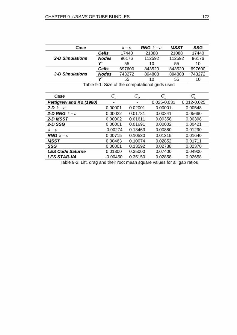
CHAPTER 9. URANS OF TUBE BUNDLES
172
Case k ε− RNG k ε− MSST SSG Cells 17440 21088 21088 17440 Nodes 96176 112592 112592 96176 2-D Simulations Y+ 55 10 55 10 Cells 697600 843520 843520 697600 Nodes 743272 894808 894808 743272 3-D Simulations Y+ 55 10 55 10
Table 9-1: Size of the computational grids used
Case LC DC LC ′ DC ′ Pettigrew and Ko (1980) - - 0.025-0.031 0.012-0.025 2-D k ε− 0.00001 0.02001 0.00001 0.00548 2-D RNG k ε− 0.00022 0.01731 0.00341 0.05660 2-D MSST 0.00002 0.01611 0.00358 0.00398 2-D SSG 0.00001 0.01691 0.00002 0.00421 k ε− -0.00274 0.13463 0.00880 0.01290 RNG k ε− 0.00715 0.10530 0.01315 0.01640 MSST 0.00463 0.10074 0.02852 0.01711 SSG 0.00001 0.13592 0.02738 0.02370 LES Code Saturne 0.01300 0.35000 0.07400 0.04900 LES STAR-V4 -0.00450 0.35150 0.02858 0.02658
Table 9-2: Lift, drag and their root mean square values for all gap ratios
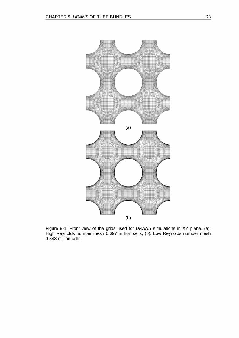
CHAPTER 9. URANS OF TUBE BUNDLES
173
(a)
(b)
Figure 9-1: Front view of the grids used for URANS simulations in XY plane. (a): High Reynolds number mesh 0.697 million cells, (b): Low Reynolds number mesh 0.843 million cells
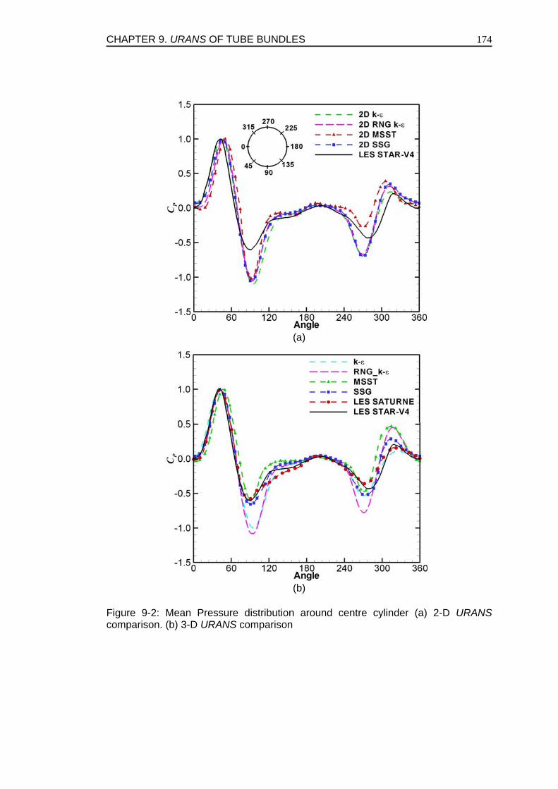
CHAPTER 9. URANS OF TUBE BUNDLES
174
(a)
(b)
Figure 9-2: Mean Pressure distribution around centre cylinder (a) 2-D URANS comparison. (b) 3-D URANS comparison
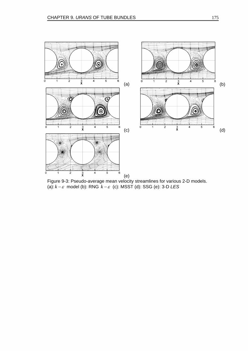
CHAPTER 9. URANS OF TUBE BUNDLES
175
(a) (b)
(c) (d)
(e)
Figure 9-3: Pseudo-average mean velocity streamlines for various 2-D models. (a): k ε− model (b): RNG k ε− (c): MSST (d): SSG (e): 3-D LES
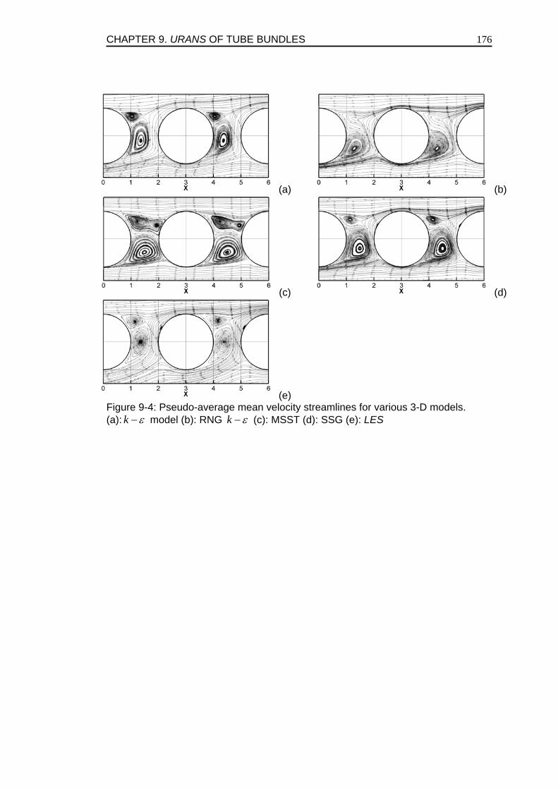
CHAPTER 9. URANS OF TUBE BUNDLES
176
(a) (b)
(c) (d)
(e)
Figure 9-4: Pseudo-average mean velocity streamlines for various 3-D models. (a): k ε− model (b): RNG k ε− (c): MSST (d): SSG (e): LES
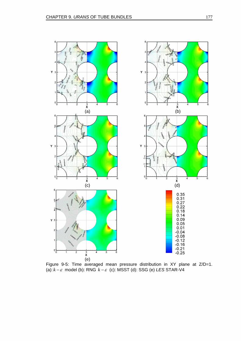
CHAPTER 9. URANS OF TUBE BUNDLES
177
(a)
(b)
(c)
(d)
(e)
Figure 9-5: Time averaged mean pressure distribution in XY plane at Z/D=1. (a): k ε− model (b): RNG k ε− (c): MSST (d): SSG (e) LES STAR-V4
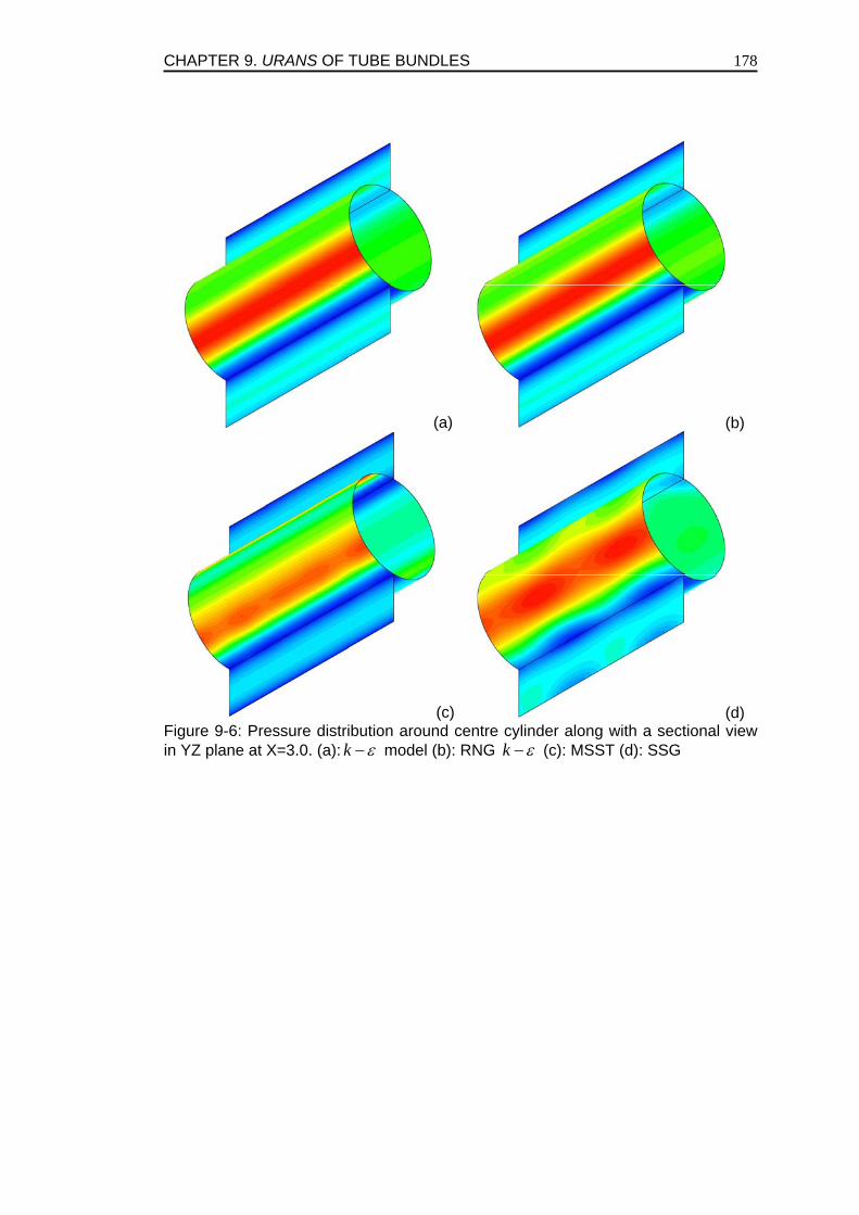
CHAPTER 9. URANS OF TUBE BUNDLES
178
(a) (b)
(c) (d)Figure 9-6: Pressure distribution around centre cylinder along with a sectional view in YZ plane at X=3.0. (a): k ε− model (b): RNG k ε− (c): MSST (d): SSG
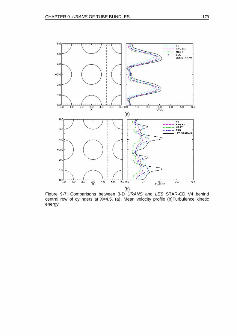
CHAPTER 9. URANS OF TUBE BUNDLES
179
(a)
(b) Figure 9-7: Comparisons between 3-D URANS and LES STAR-CD V4 behind central row of cylinders at X=4.5. (a): Mean velocity profile (b)Turbulence kinetic energy
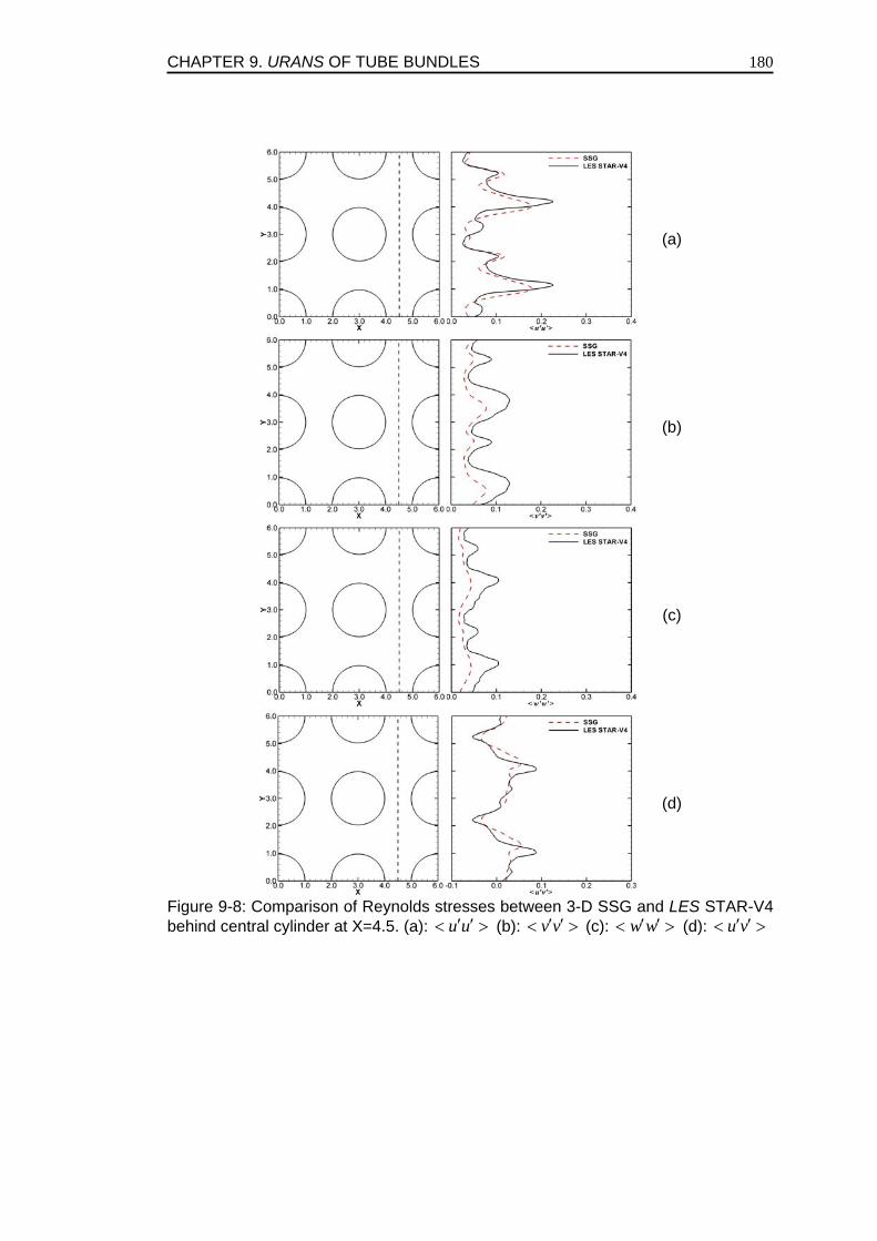
CHAPTER 9. URANS OF TUBE BUNDLES
180
(a)
(b)
(c)
(d)
Figure 9-8: Comparison of Reynolds stresses between 3-D SSG and LES STAR-V4 behind central cylinder at X=4.5. (a): u u′ ′< > (b): v v′ ′< > (c): w w′ ′< > (d): u v′ ′< >
CHAPTER 9. URANS OF TUBE BUNDLES
181
BIBLIOGRAPHY Benhamadouche, S., Laurence, D., 2003. LES, coarse LES, and transient RANS comparisons on the flow across tube bundle. Int. J. Heat Fluid Flow. 4, 470-479. Bouris, D., Bergeles, G. 1999. Two dimensional Time Dependent Simulation of the Subcritical Flow in a Staggered Tube Bundle using a Subgrid-scale Model. Int. J. Heat Fluid Flow. 20:2, 105-114. Ferziger, J.H., Peric, M. 2002. Computational Methods for Fluid Dynamics. Springer, third edition. Hanjalic, K., Kenjeres, S. 2006. RANS-Based very Large Eddy Simulation of thermal and magnetic convection of extreme condition. ASME. Vol 73, 430-440. Meyer, K.E. 1994. Experimental and Numerical Investigation of Turbulent Flow and Heat Transfer in Staggered Tube Bundles. Ph. D. Thesis, AFM 94-03, Tech. Univ. of Denmark. Pettigrew, M.J., Ko, P.L. 1980. A Comprehensive Approach to avoid Vibration and Fretting in Shell-and-Tube Heat Exchangers. Flow induced vibration of power plant components, PVP-41, ASME publications, pp. 1-18. Rollet-Miet, P., Laurence, D., Ferziger, J. 1999. LES and RANS of Turbulent Flow in Tube Bundles. Int. J. Heat Fluid Flow. 20, 241-254. Sebag, S., Maupu, V., Laurence, D. 1991. Non-Orthogonal Calculation Procedures using Second Moment Closures, TSF 8.
CHAPTER 10. LES OF GENERIC CAR MIRROR
182
Chapter 10 . LES OF FLOW AROUND A GENERIC CAR MIRROR The flow structure around a generic side mirror of a car is numerically investigated via Large Eddy Simulation (LES) incorporating polyhedral meshes. This complex geometry of the car mirror can be simplified as a half cantilever cylinder mounted vertically on a flat plate with the free end of the cylinder tapered by quarter of a sphere. The aspect ratio (AR) defined as height to radius of the cylinder is 3 and the Reynolds number (Re) based on cylinder diameter and free stream velocity is 3.2 x 10⁵. The aim of the current study is not only to model the generic car mirror via LES using polyhedral meshes but also to compute the fluctuating pressure spectrum for prediction of noise generation. LES has been an obvious choice for the simulation as it is very suitable for bluff body flows with small effects of boundary layers. The current geometry clearly requires an unstructured mesh. The central differencing scheme holds better kinetic energy conservation properties on polyhedral cells than on non-conforming tetrahedral cells. Three different grids were tested and a final mesh of 1.9 million cells was chosen with local prismatic layer refinements near the cylinder body, its immediate wake and the flat plate. The flow was found to be fully 3 dimensional with an upstream laminar separation. Pressure spectra were monitored at particular locations upstream of the body and in its wake. Flow parameters such as velocities and stresses were also computed and were found to be in good agreement with experimental data.
10.1). INTRODUCTION Over the years modern automobiles have transformed from simple transportation devices to comfortable luxury vehicles. This transformation has gone through a lot of changes; improvements in vehicle control, reduction in manufacturing cost, passenger safety, ergonomics and passenger comfort. One directly impacting factor in the comfort of passengers is the level of noise generated by the vehicle. Although for a typical car the main source of noise generation is the engine itself, however, any extremities such as side mirrors, antennas and/or overhead opening and closing sunroofs also have a significant impact in the total noise generation. From a performance point of view these extremities can contribute to a lot of drag. For a family car user this means additional fuel consumption leading to lower economy rates,
CHAPTER 10. LES OF GENERIC CAR MIRROR
183
whereas for a race or sporting car user this mean a decrease in top speed and hence performance. Yet one more criteria for the design of these extremities such as car mirrors is their appearance. Certainly modern cars users are not only concerned about the economy but also of the ergonomics of the road vehicle. Thus the external aerodynamic design of any typical car is by no means an easy job. One of the biggest sources of noise and drag in road vehicles is the side mirrors of the cars. The A-pillar-cylinder junction generally leads to substantial levels of noise generation and can cause a lot of annoyance to both car passengers and the road side pedestrians. From a performance point of view the contribution of a generic side mirror to total drag of a car is around 3-6%, hence one of the five major contributors in total drag of a car; Bernard (1988). For the side mirrors just performance and quality are not the only issues, since the side mirror itself is a guidance tool for the driver it has equal importance from a safety point of view. This means an additional constraint in the design of the side mirrors; the surface area of the reflection side. Under the current circumstances, the numerical simulation of a car mirror both from a performance and a quality point of view seems equally important.
10.2). LITERATURE REVIEW Form an acoustic point of view an interesting study at a relatively high Reynolds number is the one of Ono et al. (1999). The main idea behind this study is the redesign of a specific side mirror of a car to reduce the noise generation. Experimental measurements were performed in Nissan’s full scale low noise wind tunnel at a Reynolds number of 2 x 10⁶ over a complete Nissan road vehicle. A series of corresponding numerical computations were then performed over 3 different meshes using finite differencing techniques. The numerical grids used were of 185 x 199 x 87, 200 x 145 x 98 and 185 x 119 x 87. For the final grid an additional overlapping gird with dimensions of 106 x 69 x 70 was used for the side mirror. For this study the inlet velocity was kept at 80 Km/hr and a yaw angle of 10 degrees was taken into account for any side winds which the road vehicle might encounter on a normal cruise. This study not only looks upon the sound fluctuation levels on the surface of the mirror but also investigates the sound pressure levels away from the mirror near the passenger seat and some distance away from the vehicle. For the pressure sound level computations the Lighthill-Curl acoustic analogy is used. Since the flow is still considered to be incompressible and at a low Mach number only the dipole terms are kept for the acoustic calculations. Watkins and Oswald (1999) perform another interesting experimental study in which the authors use hot-wire anemometry to study the flow physics of a side mirror of a car from a vibrational point of view. The experiments were carried out in a closed return wind tunnel at a free stream velocity of 80-130 km/hr. Once again the authors here take into consideration the side winds for any road vehicle and thus test the configuration at different yaw angle ( 06± ). The experimental study concludes that the local velocities for this configuration can be as high as 60% or as low as 40% of the free
CHAPTER 10. LES OF GENERIC CAR MIRROR
184
stream velocity whereas the local turbulence intensity can be as high as 40% even at cruise speeds. Even though the results seem to be very promising for the two aforementioned experimental and numerical studies, yet use of a certain type of side mirror shape in conjunction with a full scale car model makes the availability of numerical and experimental data somewhat less useful from a general perspective. From an academic point of view a more generic side mirror shape would better serve our purpose which would not only give a better understanding of the flow physics but would also serve as a benchmark for acoustic calculations at a later stage. One such numerical study is from Rung et al. (2002) in which the authors compare DES with Unsteady Reynolds Averaged Navier Stokes (URANS) for a generic side mirror mounted vertically on a flat plate at a moderate Reynolds number of 5.2 x10⁵. The acoustic calculations are based on Ffowcs-Williams and Hawkings (FWH) analogy and sound pressure fluctuation levels are shown at various locations on the mirror surface and flat plate. The authors conclude that the DES shows a remarkable improvement over traditional URANS for moderate computational grids. As for the flow physics point of view the paper also shows the normalized pressure profile over the surface of the mirror. This data shall later be used for comparison. Perhaps the most intense numerical study for a generic side mirror is the one conducted by Ask and Davidson (2006). The authors test a generic car mirror on a flat plate with a Reynolds number of 5.2 x 10⁵. Although such a high Reynolds number is considered to be a critical Reynolds number for both cylinder and sphere flows, the author’s inference suggests otherwise. DES and LES studies are conducted on identical grids with the incompressibility assumption. It is found that LES results showed marked improvement over the widely popular DES results especially in terms of Pressure fluctuation levels. For the DES results the instantaneous drag coefficient profile is seen to be lacking high frequency content when compared to the LES drag profile. The mirror mean surface pressure values are still found comparable by the two numerical techniques. The aforementioned studies of Rung et al. (2002) and Ask and Davidson et al. (2006) both use the experimental and numerical data of Hold et al. (1999) and Siegert et al. (1999). The experimental measurements and numerical computations are performed essentially for the same Reynolds number of 5.2 x 10⁵. For the numerical simulations Baldwin-Lomax model has been used whereas for the experimental measurements the aeroacoustic wind tunnel at FKFS Stuttgart is utilized. A more recent study on the redesign of a generic side mirror has been conducted by Grahs and Othmer (2006). The authors use two different numerical techniques DES and SAS (Scale Adaptive Simulation) over two different types of meshes; a hexahedral fully conforming mesh and a hybrid non-conforming mesh. The use of this second type of mesh is highly encouraged by the authors since for the redesigning of the mirror shape only the internal non-conforming mesh has to be remade.
CHAPTER 10. LES OF GENERIC CAR MIRROR
185
10.3). CASE DESCRIPTION AND NUMERICS The generic car mirror mounted on a flat plate consists of a half cylinder complemented by a quarter sphere at the tip. The cylinder and sphere diameters (D) are 0.2 meters whereas the cylinder height is 1 D, making the total height of the mirror 1.5 D. The inlet domain is 4.5 D upstream of the mirror whereas the outlet is 14 D downstream. The spanwise ( y ) farfield boundaries are positioned at 5.5 D on each side of the mirror. The top (normal z ) farfield boundary is kept at 7 D as shown in Figure 10-1. The inlet velocity is fixed at 26 m/s and the corresponding Reynolds number ( ReD ) is 3.2 x 10⁵. For the simulations no artificial perturbations are prescribed at the inlet. Due to the complex shape of the geometry a totally conforming regular mapped mesh would have been too complex to generate and computationally very expensive. An alternative solution could have been a tetrahedral mesh. Tetrahedral meshes have a number of advantages such as they are fairly easy to generate using any available automatic mesh generator. Moreover, since they are the simplest of elements their face and volume centred locations are well defined. However, on a global level with a tetrahedral mesh one would end up with a huge number of cells for a geometry like the one under consideration. This is so because tetrahedral control volumes cannot be stretched too much. It was thus decided to test non-conforming polyhedral meshes. The automatic mesh generator from CD-adapco STAR-Design was used for creating a polyhedral mesh. The mesh was generated in individual blocks and was later assembled by multi-block transformation technique. Three different meshes with varying dimensions were used as shown in Table 10-1. The Coarse Mesh (CM) contains 0.4 million cells, 1.4 million nodes and around 2 million faces. The geometry in this case is wrapped around by a fine mesh block (CF1) which progressively becomes coarser as we move away from the mirror body. This CF1 is encased inside a much coarser computational domain. The total number of cells inside the CF1 block are 0.25 million. The Medium Mesh (MM) contains 0.8 million cells, 4 million nodes and 5 million faces. The grid in this case is also made on the same principle as the CM but the total number of cells inside the fine mesh block (MF1) are 0.5 million. For the Fine Mesh (FM) the number of cells is 1.9 million, number of nodes is 8.8 million and number of faces is 11.2 million. The mirror geometry in the FM case is encapsulated inside two fine blocks instead of one; a very fine mesh block (FF1) just around the body containing 0.55 million cells and a fine mesh block (FF2) encasing the FF1 block containing 0.45 million cells. These two blocks are then encapsulated by a combination of multiple blocks just like in the case of CM and MM. For all the three meshes CM, MM and FM the
CHAPTER 10. LES OF GENERIC CAR MIRROR
186
encapsulating block dimensions are given in Table 10-2. The location of these inner encapsulating blocks and their meshes are shown in Figure 10-2 along various cross sectional views. Various zoomed-in views for the Fine Mesh (FM) are shown in Figure 10-3. An inter-dependent boundary layer meshing technique is used for all the three meshes near the mirror body and flat plate. This is done by using a prism layer of regular orthogonal cells, a close up of this prism layer can be seen from Figure 10-3(c). This prism layer contains at least 20 cells in the wall normal direction. For the Fine mesh near the mirror surface viscous sublayer is assumed to be resolved where the Y+ is close to 1. However, no attempt has been made to resolve the boundary layer over the flat plate as this would have increased the computational requirements considerably making the simulation impossible given the available computer resources. For the numerical simulation the standard Smagorinsky model is used where the constant is set to 0.065. For spatial discretizations the 2nd order central differencing scheme is used whereas for time discretizations the three time level implicit time advancing scheme (TTLM) described in Ferziger and Peric (2002) is used with a time step of 2.5 x 10⁻⁴. The total simulation time was 18 flow through cycles and collection of statistics was done over the last 10 cycles to ensure adequate time averaging of flow parameters. As already discussed conserving kinetic energy not only eliminates numerical diffusion, but also ensures a bounded solution even with second order pure central differencing schemes, such as those used here. In the far field the grid is considerably coarser, this can result in undesirable artificial numerical wiggles when using central differencing schemes especially for non-conforming unstructured grids; Ferziger and Peric (2002). To overcome this issue the central scheme is locally blended with first order upwinding in the region far away from mirror. Although such a procedure ensures boundedness and avoids numerical instabilities, it also leads to some amount of dissipation. However, since the primary area of interest in the current study is close to the body such a practice should not have much adverse effects near wake and should not alter the reliability of the results. For the current simulations a constant velocity inlet with no artificial perturbations is implemented. For the far fields such as the ones in the spanwise directions and the top domain, slip boundary conditions are prescribed. Whereas close to the outlet domain a high amount of blending is done between central differencing and upwinding to avoid any sort of reverse flow. It is assumed that the outlet domain is sufficiently far downstream of the body and any such artificial blending would not dampen the flow parameters or kinetic energy in the area of our interest which is close to the mirror body.
10.4). RESULTS AND DISCUSSIONS Polyhedral cells clearly have marked advantages over the regular tetrahedral cells. For example a tetrahedral cell will only have three or four neighbours which can in some cases lead to problems while computing gradients at cell centres. Additionally corner cells might end up with only two or sometimes

CHAPTER 10. LES OF GENERIC CAR MIRROR
187
even one neighbour, which could lead to serious numerical instabilities and inaccuracies. On the other hand polyhedral cells have a lot of neighbours typically around 10 or more which allows for a reasonable prediction of both gradients at cell centres and local flow directions. However, on a negative side more neighbours for every cell mean a higher storage space and computing requirements per degree of freedom, but tests at Manchester University and those conducted at CD-adapco confirm that the added computing expenditure is more than compensated by the higher accuracy and quick convergence of results. Second order accuracy is retained for polyhedral meshes much like Cartesian structured grids for simple approximations such as mid-point rule and linear interpolation. However, the cells are required to hold basic mesh properties correctly such as skewness, flatness and orthogonalities which at times are difficult to identify on polyhedral meshes let alone be correctly catered for. For tetrahedral meshes on the other hand special approximations are required to hold equally good accuracy; Peric (2004). The conservation of kinetic energy is a critical issue for any DNS or LES simulation, addressed in detail by Benhamadouche and Laurence (2002) for unstructured meshes. Indeed polyhedral meshes (considered to be unstructured meshes) need to behave in a similar fashion. Both Peric (2004) and Moulinec et al. (2005) show that polyhedral meshes hold kinetic energy conservation far superior than tetrahedral meshes. Moulinec et al. (2005) tested polyhedral meshes for a U-bend which showed a good comparison with experimental data. For the car mirror configuration a regular Cartesian gird is hard to generate taking into consideration the cell stretching close to outer walls near the bend. Peric (2004) shows more basic tests on retaining kinetic energy over a flat 2-D surface. Results indicate the same that polyhedral meshes conserve kinetic energy much like the Cartesian Hexahedral meshes but with much lower number of cells (approximately half). For the same geometry for tetrahedral cells clearly one needs additional special discretizations to conserve this kinetic energy.
10.4.1). FLOW PHYSICS For the current Re number of 3.2 x 10⁵, the corresponding inlet velocity is 26 m/s which gives a Mach number of 0.08. Incompressibility is assumed with reliability since both experiments and numerical simulations performed at a slightly higher Mach number of 0.11 also hold this condition true; see Hold et al. (1999), Rung et al. (2002) and Ask and Davidson (2006). The flow over the generic car mirror is an open vortex flow showing full three dimensionality with a laminar upstream separation. The approaching flow is seen to be fully symmetrical with no variance in the flow incidence angle. The stagnation point is located at zero degrees for both the cylinder and the sphere bodies. The laminar separation can best be seen by the oil flow visualizations of the experiments shown in Figure 10-4(a) which are taken from Ask and Davidson (2006). The measurements are made at a Reynolds number of 5.2 x 10⁵ and
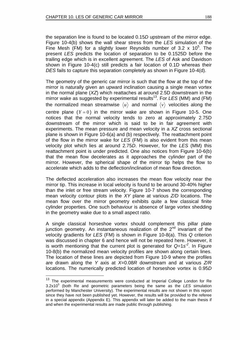
CHAPTER 10. LES OF GENERIC CAR MIRROR
188
the separation line is found to be located 0.15D upstream of the mirror edge. Figure 10-4(b) shows the wall shear stress from the LES simulation of the Fine Mesh (FM) for a slightly lower Reynolds number of 3.2 x 10⁵. The present LES predicts the location of separation to be 0.1525D before the trailing edge which is in excellent agreement. The LES of Ask and Davidson shown in Figure 10-4(c) still predicts a fair location of 0.1D whereas their DES fails to capture this separation completely as shown in Figure 10-4(d). The geometry of the generic car mirror is such that the flow at the top of the mirror is naturally given an upward inclination causing a single mean vortex in the normal plane (XZ) which reattaches at around 2.5D downstream in the mirror wake as suggested by experimental results13. For LES (MM) and (FM) the normalized mean streamwise u and normal v velocities along the centre plane ( 0=Y ) in the mirror wake are shown in Figure 10-5. One notices that the normal velocity tends to zero at approximately 2.75D downstream of the mirror which is said to be in fair agreement with experiments. The mean pressure and mean velocity in a XZ cross sectional plane is shown in Figure 10-6(a) and (b) respectively. The reattachment point of the flow in the mirror wake for LES (FM) is also evident from this mean velocity plot which lies at around 2.75D. However, for the LES (MM) this reattachment point is under predicted. One also notices from Figure 10-6(b) that the mean flow decelerates as it approaches the cylinder part of the mirror. However, the spherical shape of the mirror tip helps the flow to accelerate which adds to the deflection/inclination of mean flow direction. The deflected acceleration also increases the mean flow velocity near the mirror tip. This increase in local velocity is found to be around 30-40% higher than the inlet or free stream velocity. Figure 10-7 shows the corresponding mean velocity contour plots in the XY plane at various Z/D locations. The mean flow over the mirror geometry exhibits quite a few classical finite cylinder properties. One such behaviour is absence of large vortex shedding in the geometry wake due to a small aspect ratio. A single classical horseshoe vortex should complement this pillar plate junction geometry. An instantaneous realization of the 2nd invariant of the velocity gradients for LES (FM) is shown in Figure 10-8(a). This Q criterion was discussed in chapter 6 and hence will not be repeated here. However, it is worth mentioning that the current plot is generated for Q=1s-2. In Figure 10-8(b) the normalized mean velocity profiles are shown along certain lines. The location of these lines are depicted from Figure 10-9 where the profiles are drawn along the Y axis at X=0.08R downstream and at various Z/R locations. The numerically predicted location of horseshoe vortex is 0.95D 13 The experimental measurements were conducted at Imperial College London for Re 3.2x10⁵ (both Re and geometric parameters being the same as the LES simulation performed by Manchester University). The experimental results are not shown in this report since they have not been published yet. However, the results will be provided to the referee in a special appendix (Appendix E). This appendix will later be added to the main thesis if and when the experimental results are made public through publishing.
CHAPTER 10. LES OF GENERIC CAR MIRROR
189
(1.9R) in the spanwise (Y) direction also shown as dashed horizontal line in Figure 10-8(b). The concave curve at this particular location in top profile (Z/R=0.1) in Figure 10-8(b) marks this location. Interestingly the experimental measurements show this location to be 0.925D in spanwise direction which is once again an excellent match. For the Iso-Q structures shown in Figure 10-8(a) one notices not only the existence and location of a horseshoe vortex but also the large structures in the mirror wake. Unfortunately due to unavailability of a proper post-processor for polyhedral meshes the numerical LES data had to be interpolated onto a mapped mesh. Once the mapping was done the Iso-Q were then generated and polished. This however, is an approximate solution to the problem which leads to some numerical interpolation errors resulting in undesirable dampening of the fine structures in the immediate wake of the mirror. However, most of the larger structures are still visible depicting an excellent representation of the flow behaviour. In particular, we can see a succession of 4 arch shaped vortices, the first one about 0.2D downstream of, and almost parallel to the sharp edge of the mirror, and emerging from the unsteady shear layer. About 0.25D downstream we see that the 3 succeeding arched structures are being toppled over by the downwash motion. To measure the mean pressure on the cylinder surface a number of sensor locations were predefined. These locations cover mainly the edge of the mirror, the front side and some area of the back side. The actual locations of the sensors are given in Table 10-3. A graphical representation of the location of these sensors is then shown in Figure 10-10(a) and (b). Note from these two figures that the sensors from 1-9 are actually located at the mirror edge which is YZ plane. The sensors 10-20 are located along the symmetry line on the front of the mirror in XZ plane whereas sensors 26-34 are all on the leeward side of the mirror. The mean pressure profile (CP) for these sensor locations is then shown in Figure 10-10(c). Where (CP) is defined as
202( ) /P refC p p Uρ= − and the reference pressure pref is set to zero. The
sensor locations 1-9 which are on the edge of the mirror actually lie downstream of the separation zone and hence show a constant CP profile. On the other hand sensors 10-11 and 24-25 actually lie just before this separation zone and hence show a slight dip in CP profile. Sensors 12-23 lie on the front side of the mirror and hence show an increase in CP values. The stagnation region is also evident from this curve which is shown by the constant CP=1 values at sensor locations 16-20. One also notices from Figure 10-10(c) that even though the experimental data (Hold et al. (1999)) which is at a slightly higher Re number of 5.2 x 10⁵ shows a fair agreement with the numerical LES (FM) results. The instantaneous drag (CD), lift (CL) and side (CS) forces on the mirror surface are shown in Figure 10-11. The profiles are drawn against the non-dimensionalised time scale which is 0 /tU D . One notices that the drag coefficient is around 0.6 whereas the lift coefficient is around zero. The side force which in this case is along the axis (Z) of the mirror is also shown in this figure which is around 15% of the drag force.
CHAPTER 10. LES OF GENERIC CAR MIRROR
190
10.4.2). ACOUSTIC CALCULATIONS The aero-acoustic analysis for a noise generating object present in a flow field was initially proposed by Lighthill (1952). Curle (1955) and then later Ffwocs Williams and Hawkings (1965) proposed modifications to Lighthill analogy to account for presence of solid walls. These analogies convert the governing equation of continuity and momentum to an inhomogeneous wave equation which is given as
( ) ( ) 22 2
202 2
ρ ρ ρ δ δ∂∂ ∂ ∂ ∂
− = − +∂ ∂ ∂ ∂ ∂ ∂
ijn ij
i i i j
Tc v f p f
t x t x x x (10.1)
here ( )2ρ τ ρ δ= − + −ij i j ij ijT u u p c and is known as the Lighthill tensor where c is the speed of sound. The terms on the right hand side of equation (10.1) are the monopole, dipole and quadrupole source terms respectively. Generally for a stationary surface one can neglect the monopole term. For an incompressible case such as the one under consideration where the Mach number is small ( 0.2<Ma ) the quadrupole term is also ignored since its contribution is about 0.01% in comparison to the contribution of the dipole term; Grahs and Othmer (2006). This leaves us only with the dipole term which contains the direct effects of pressure fluctuations on the solid surface. The sound generation can thus be represented as either the pressure fluctuation level (PFL) or by sound pressure levels (SPL) which are given as
2 2
10 102 20 0
( , ) ( , )( ) 10 log , ( ) 10 logsf rms rmsp y t p x tPFL y SPL xp p
⎛ ⎞ ⎛ ⎞= =⎜ ⎟ ⎜ ⎟⎜ ⎟ ⎝ ⎠⎝ ⎠
(10.2)
where y is the surface location where the pressure fluctuations are being monitored and x is the position vector of the observer. The reference pressure 0p in both these cases is set to 2 x10⁻⁵. For the current case only the PFLs are computed at a few locations since our primarily interest is in the magnitude of source of sound generation. The PFLs for three different locations are shown in Figure 10-12 to Figure 10-14. The corresponding sensor locations are shown in Table 10-4. The sensors 116 and 119 are both located on the centreline in the XZ plane on the surface of the flat plate. Sensor 116 is located 0.6D upstream of the body whereas sensor 119 is located 1D downstream. These figures show the pressure fluctuations in decibel (dB) which is shown against the log scale of frequency (Hz). Acoustic data was collected for 12 seconds which corresponds to a data set of 48,000 values for every sensor location. This data set was then averaged over 7 equal windows to make the mean somewhat smooth to get a better estimate of the PFLs. The red dashed lines in these figures show the actual computed PFLs for the LES (FM) case at a Re number of 3.2 x 10⁵. However, since the experimental data is at a much higher Re number of 5.2 x 10⁵, the numerical data has to be translated by 8.5 dB which is in accordance with the Re number adjustment. Since the dynamic pressure is related to the free stream velocity as 2
0 / 2P Uρ= , the
CHAPTER 10. LES OF GENERIC CAR MIRROR
191
pressure fluctuations can then be related as 20P U′ ∝ . However, since we are
interested in the square of the pressure fluctuations the scaling then becomes 2 4
0P U′ ∝ . Now since the ratio between experimental and numerical inlet velocities is exactly 1.625 ( 0 0/ 1.625Exp NumU U = ), the square of the pressure fluctuations have to translated exactly 8.5 dB ( 1010 log (6.97) 8.5= ). The translated numerical data is shown as solid green lines in Figure 10-12 to Figure 10-14. A slight discrepancy still exists between the numerical and measured data, however, it can be attributed to the comparatively coarse grid on the bottom flat plate, which was not properly resolved taking into consideration the increase in computational cost. Since the grid in the wake of the mirror near sensors 119 and 123 is finer than the grid near the sensor 116, the comparison of the two former locations is still somewhat better than the comparison of the latter.
10.5). CONCLUSIONS In the current study an attempt was made to fully investigate the flow behaviour over a generic car mirror. Incompressibility was assumed for all simulations since the Mach number is sufficiently small. Polyhedral cells were used for the first time with LES on such a complex geometry to test its capabilities. Three different meshes were tested 0.4 million, 0.8 million and 1.9 million. The results from 1.9 million mesh seemed to be the closest to the available experimental measurements. The flow field was found to have a laminar separation 0.15D upstream of the mirror edge. The flow shows almost no classical Karman vortex shedding due to a very small aspect ratio. However, instead one sees sharp arch shaped structures in the wake which are generated by the sharp trailing edge of the mirror. These arch structures which when originated are parallel to the mirror axis are then toppled over by the strong downwash coming from the top of the mirror. Furthermore in the close vicinity of the mirror tip the local flow field is seen to increase in velocity by around 30-40%. The reattachment point for the flow is located at around 2.75D in the mirror wake. The interaction of the classical pillar-plate junction is also observed in the form of a horseshoe vortex which is located 0.95D away from the body in both streamwise and spanwise directions. The pressure fluctuation levels were also computed at three different locations and were found to be in fair agreement with the experimental measurements.
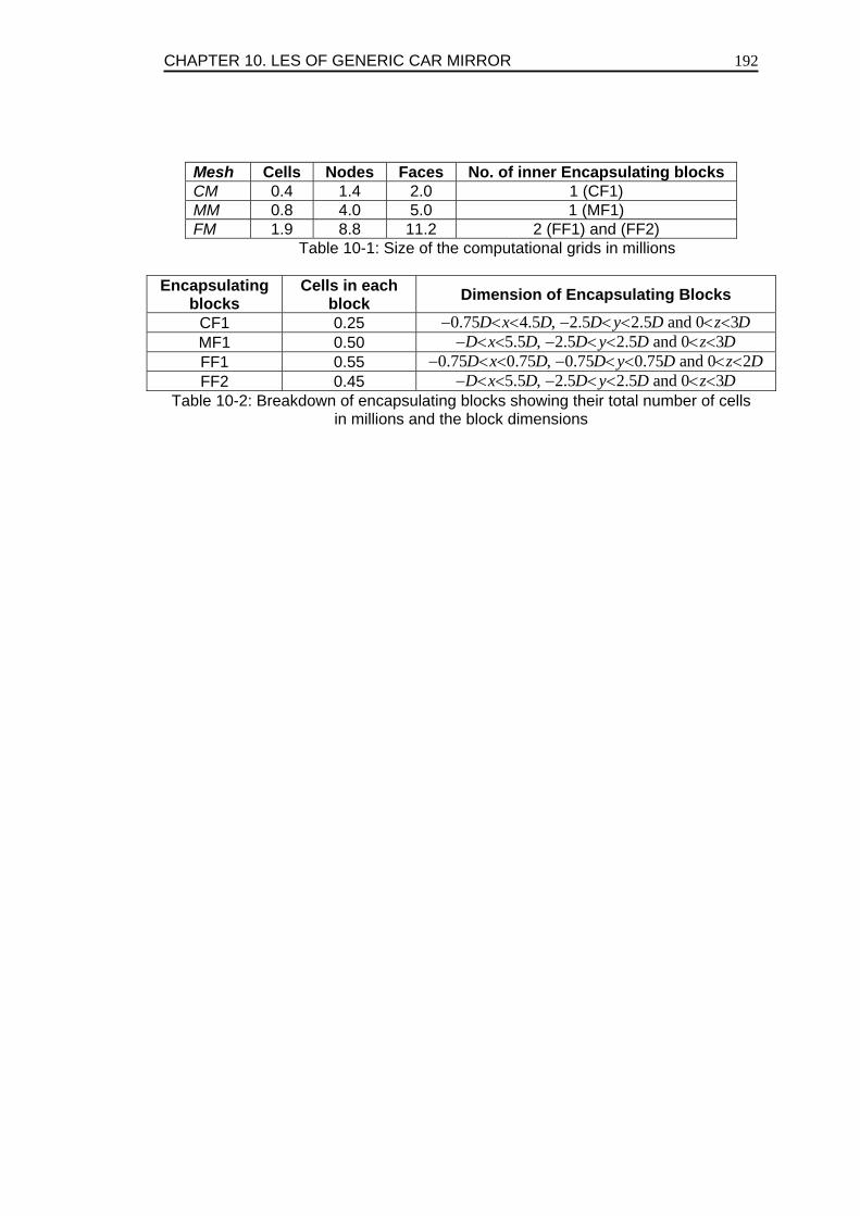
CHAPTER 10. LES OF GENERIC CAR MIRROR
192
Mesh Cells Nodes Faces No. of inner Encapsulating blocks CM 0.4 1.4 2.0 1 (CF1) MM 0.8 4.0 5.0 1 (MF1) FM 1.9 8.8 11.2 2 (FF1) and (FF2)
Table 10-1: Size of the computational grids in millions
Encapsulating blocks
Cells in each block Dimension of Encapsulating Blocks
CF1 0.25 0.75 4.5 , 2.5 2.5 and 0 3− < < − < < < <D x D D y D z D
MF1 0.50 5.5 , 2.5 2.5 and 0 3− < < − < < < <D x D D y D z D
FF1 0.55 0.75 0.75 , 0.75 0.75 and 0 2− < < − < < < <D x D D y D z D
FF2 0.45 5.5 , 2.5 2.5 and 0 3− < < − < < < <D x D D y D z D
Table 10-2: Breakdown of encapsulating blocks showing their total number of cells in millions and the block dimensions
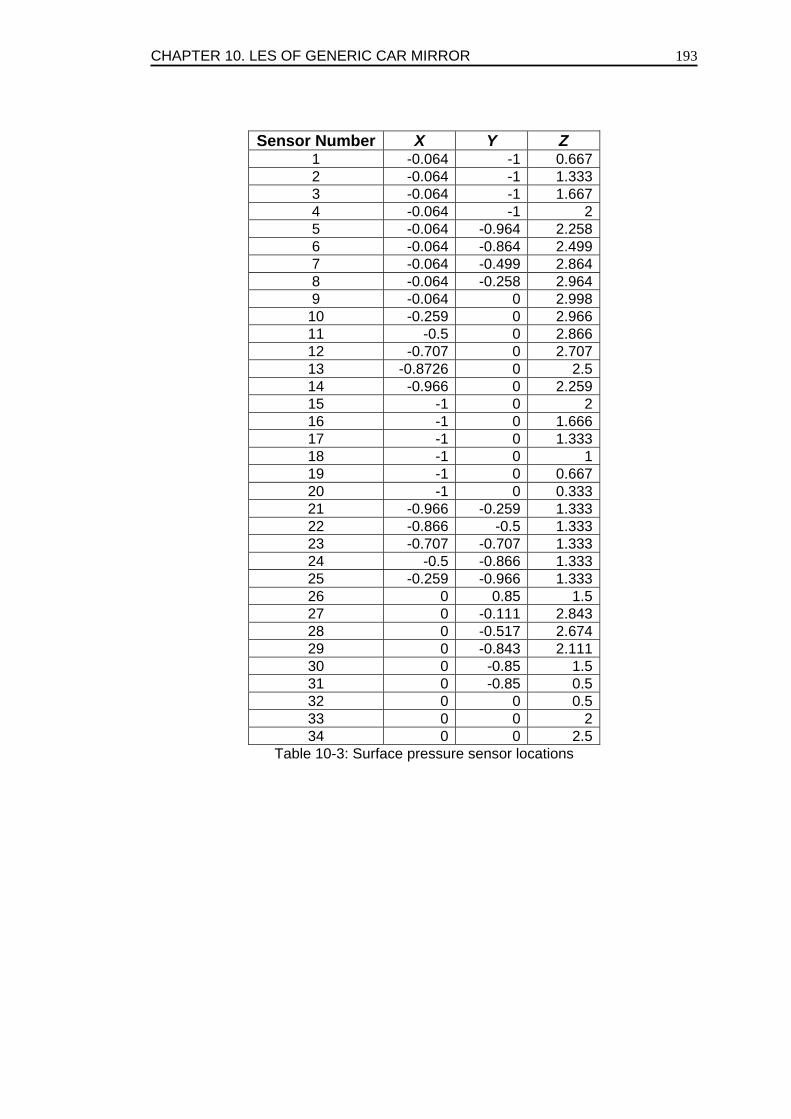
CHAPTER 10. LES OF GENERIC CAR MIRROR
193
Sensor Number X Y Z
1 -0.064 -1 0.667 2 -0.064 -1 1.333 3 -0.064 -1 1.667 4 -0.064 -1 2 5 -0.064 -0.964 2.258 6 -0.064 -0.864 2.499 7 -0.064 -0.499 2.864 8 -0.064 -0.258 2.964 9 -0.064 0 2.998
10 -0.259 0 2.966 11 -0.5 0 2.866 12 -0.707 0 2.707 13 -0.8726 0 2.5 14 -0.966 0 2.259 15 -1 0 2 16 -1 0 1.666 17 -1 0 1.333 18 -1 0 1 19 -1 0 0.667 20 -1 0 0.333 21 -0.966 -0.259 1.333 22 -0.866 -0.5 1.333 23 -0.707 -0.707 1.333 24 -0.5 -0.866 1.333 25 -0.259 -0.966 1.333 26 0 0.85 1.5 27 0 -0.111 2.843 28 0 -0.517 2.674 29 0 -0.843 2.111 30 0 -0.85 1.5 31 0 -0.85 0.5 32 0 0 0.5 33 0 0 2 34 0 0 2.5
Table 10-3: Surface pressure sensor locations
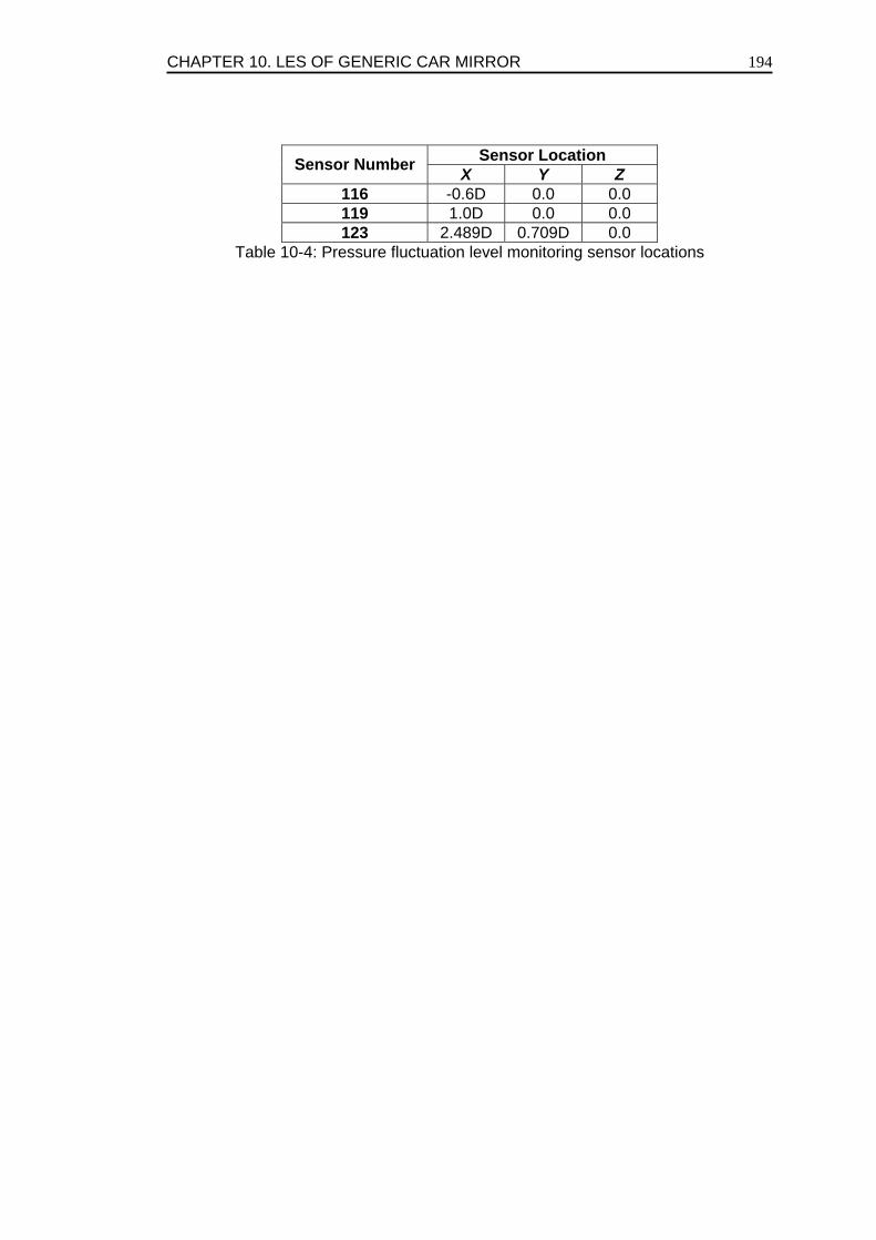
CHAPTER 10. LES OF GENERIC CAR MIRROR
194
Sensor Location Sensor Number X Y Z
116 -0.6D 0.0 0.0 119 1.0D 0.0 0.0 123 2.489D 0.709D 0.0
Table 10-4: Pressure fluctuation level monitoring sensor locations
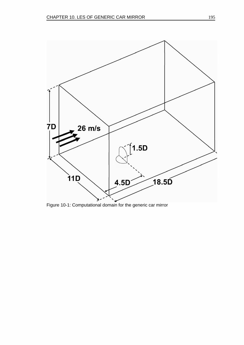
CHAPTER 10. LES OF GENERIC CAR MIRROR
195
Figure 10-1: Computational domain for the generic car mirror
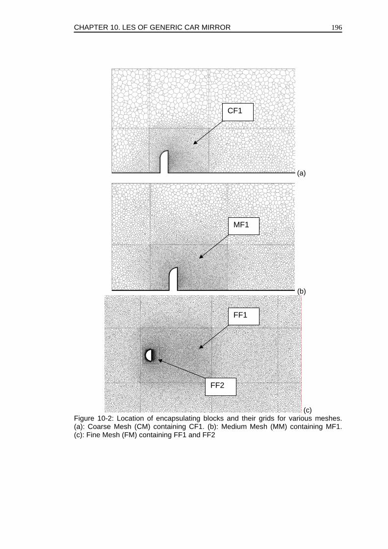
CHAPTER 10. LES OF GENERIC CAR MIRROR
196
(a)
(b)
(c) Figure 10-2: Location of encapsulating blocks and their grids for various meshes. (a): Coarse Mesh (CM) containing CF1. (b): Medium Mesh (MM) containing MF1. (c): Fine Mesh (FM) containing FF1 and FF2
CF1
MF1
FF1
FF2
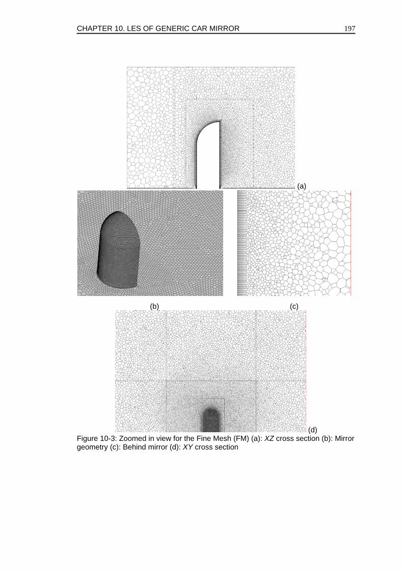
CHAPTER 10. LES OF GENERIC CAR MIRROR
197
(a)
(b) (c)
(d) Figure 10-3: Zoomed in view for the Fine Mesh (FM) (a): XZ cross section (b): Mirror geometry (c): Behind mirror (d): XY cross section
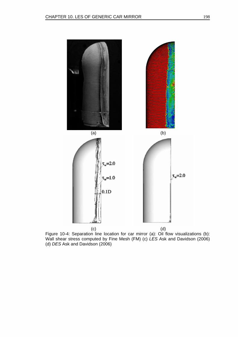
CHAPTER 10. LES OF GENERIC CAR MIRROR
198
(a)
(b)
(c)
(d)
Figure 10-4: Separation line location for car mirror (a): Oil flow visualizations (b): Wall shear stress computed by Fine Mesh (FM) (c) LES Ask and Davidson (2006) (d) DES Ask and Davidson (2006)
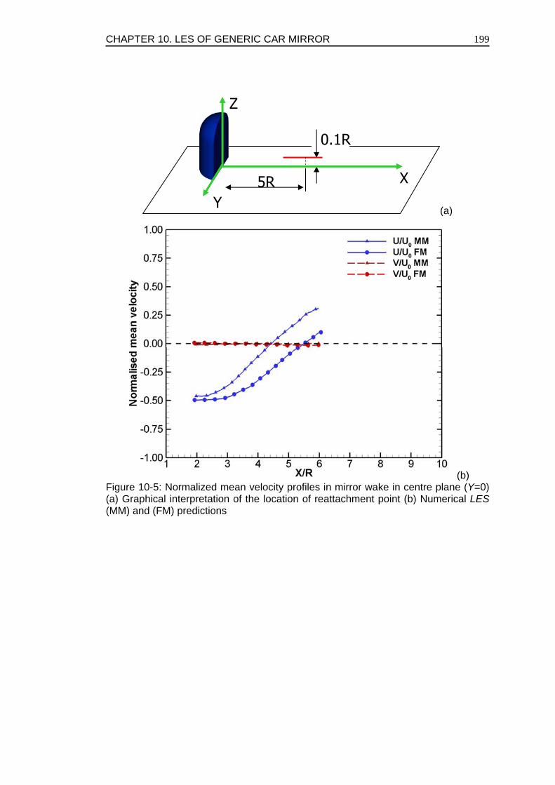
CHAPTER 10. LES OF GENERIC CAR MIRROR
199
(a)
(b) Figure 10-5: Normalized mean velocity profiles in mirror wake in centre plane (Y=0) (a) Graphical interpretation of the location of reattachment point (b) Numerical LES (MM) and (FM) predictions
5R
0.1R
X
Z
Y
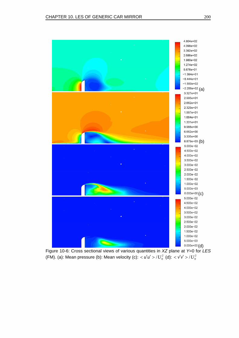
CHAPTER 10. LES OF GENERIC CAR MIRROR
200
(a)
(b)
(c)
(d) Figure 10-6: Cross sectional views of various quantities in XZ plane at Y=0 for LES (FM). (a): Mean pressure (b): Mean velocity (c): 2
0/′ ′< >u u U (d): 20/′ ′< >v v U
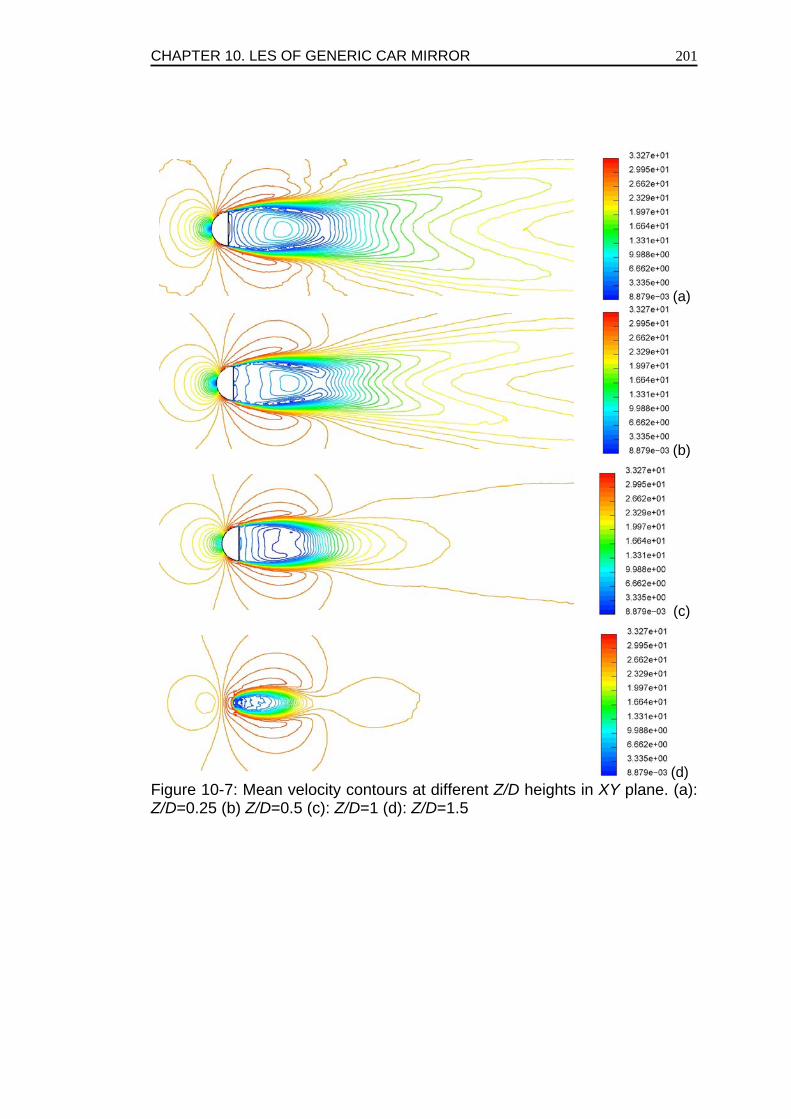
CHAPTER 10. LES OF GENERIC CAR MIRROR
201
(a)
(b)
(c)
(d) Figure 10-7: Mean velocity contours at different Z/D heights in XY plane. (a): Z/D=0.25 (b) Z/D=0.5 (c): Z/D=1 (d): Z/D=1.5
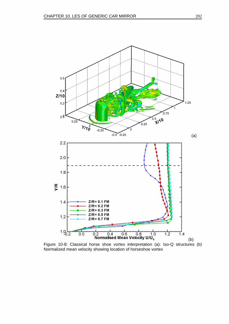
CHAPTER 10. LES OF GENERIC CAR MIRROR
202
(a)
(b) Figure 10-8: Classical horse shoe vortex interpretation (a): Iso-Q structures (b) Normalized mean velocity showing location of horseshoe vortex
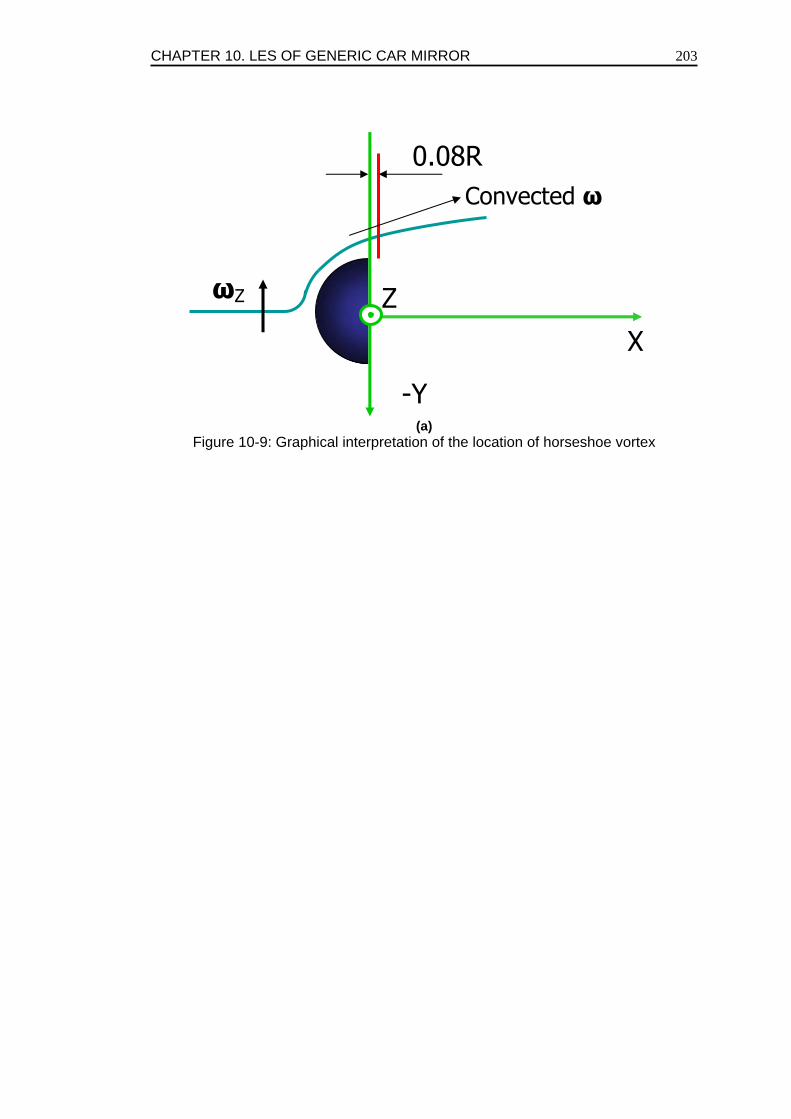
CHAPTER 10. LES OF GENERIC CAR MIRROR
203
(a)
Figure 10-9: Graphical interpretation of the location of horseshoe vortex
-Y
X
Z
0.08R
ωΖ
Convected ω
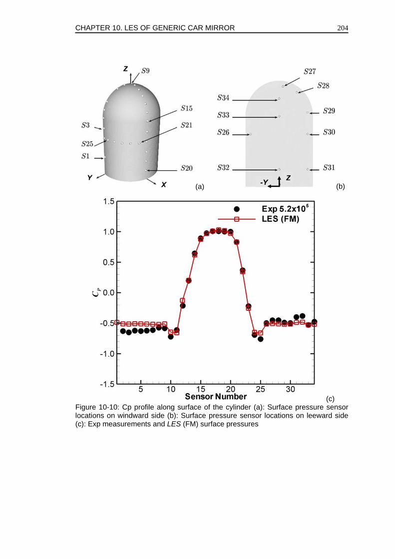
CHAPTER 10. LES OF GENERIC CAR MIRROR
204
(a) (b)
(c) Figure 10-10: Cp profile along surface of the cylinder (a): Surface pressure sensor locations on windward side (b): Surface pressure sensor locations on leeward side (c): Exp measurements and LES (FM) surface pressures
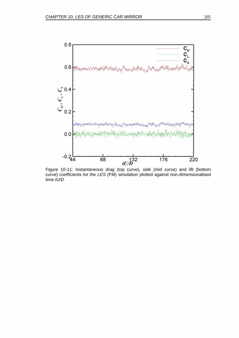
CHAPTER 10. LES OF GENERIC CAR MIRROR
205
Figure 10-11: Instantaneous drag (top curve), side (mid curve) and lift (bottom curve) coefficients for the LES (FM) simulation plotted against non-dimensionalised time tU/D
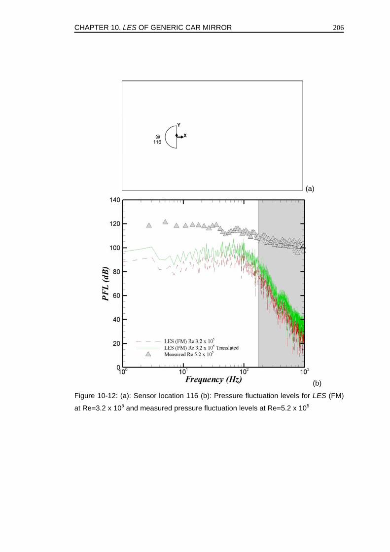
CHAPTER 10. LES OF GENERIC CAR MIRROR 206
(a)
(b)
Figure 10-12: (a): Sensor location 116 (b): Pressure fluctuation levels for LES (FM)
at Re=3.2 x 10⁵ and measured pressure fluctuation levels at Re=5.2 x 10⁵
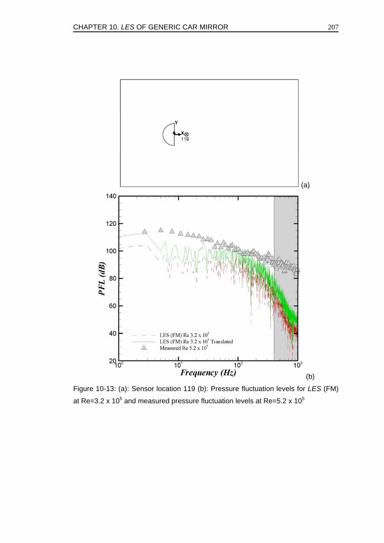
CHAPTER 10. LES OF GENERIC CAR MIRROR 207
(a)
(b)
Figure 10-13: (a): Sensor location 119 (b): Pressure fluctuation levels for LES (FM)
at Re=3.2 x 10⁵ and measured pressure fluctuation levels at Re=5.2 x 10⁵
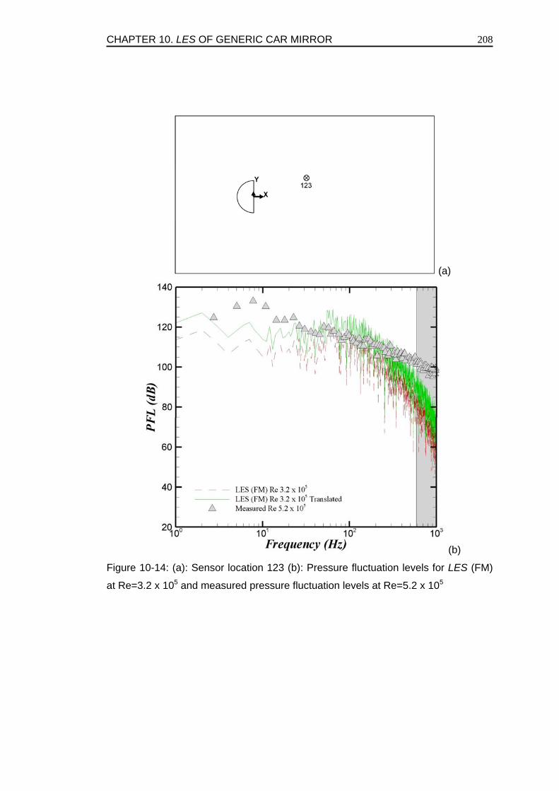
CHAPTER 10. LES OF GENERIC CAR MIRROR 208
(a)
(b)
Figure 10-14: (a): Sensor location 123 (b): Pressure fluctuation levels for LES (FM)
at Re=3.2 x 10⁵ and measured pressure fluctuation levels at Re=5.2 x 10⁵
CHAPTER 10. LES OF GENERIC CAR MIRROR
209
BIBLIOGRAPHY Ask J., Davidson, L. 2006. The Sub-critical flow past a generic side mirror and its impact on sound generation and propagation. 12th AIAA/CEAS Conf. Massachusetts. Barnard, R. H. 1988. Road Vehicle Aerodynamic Design. Longman. Benhamadouche, S., Laurence, D. 2002. Global kinetic energy conservation with unstructured Meshes. Int. J. Num. Meth. Fluids, 40. 561-572. Curle, N. 1955. The influence of solid boundaries upon aerodynamic sound. Proc. Roy. Soc. A 231, 505-514. Ferziger, J.H., Peric, M. 2002. Computational Methods for Fluid Dynamics. Springer, third edition. Ffowcs Williams, J. E., Hawkins, D. L. 1969. Sound generation by turbulence and surfaces in arbitrary motion. Philos. Trans. Roy. Soc. A 264, No. 1151,321-342. Grahs, T., Othmer, C. 2006. Evaluation of aerodynamic noise generation: Parameter study of a generic side mirror evaluating the aeroacoustic source strength. ECCOMAS CFD, Netherlands. Hold, R., Brenneis, A., Eberle, A., Schwarz, V., Siegert, R. 1999. Numerical simulation of aerodynamic sound generation by generic bodies placed on a plate: Part I-Prediction of aerodynamic sources. 5th AIAA/CEAS Conf. Washington. AIAA-99-1896. Hunt, J. C. R., Wray, A. A., Moin, P., 1988. Eddies, stream and convergence zones in turbulent flows. Report CTR-S88. Center for Turbulent Research. Lighthill, M. J. 1952. On sound generated aerodynamically. General theory. Proc. Roy. Soc. A 211, 5640587. Moulinec, C., Benhamadouche, S., Laurence, D., Peric, M. 2005. LES in U-bend pipe meshed by polyhedral cells. ERCOFTAC conference Sardinia, Elsevier. Ono, K., Himeno, R., Fukushima, T. 1999. Prediction of wind noise radiated from passenger cars and its evaluation based on auralization. J. Wind Eng. Ind. Aero. Vol 81, 403-419. Peric, M. 2004. Flow Simulation Using Control Volumes of Arbitrary Polyhedral Shape, ERCOFTAC bulletin No. 62, Page 25-29.
CHAPTER 10. LES OF GENERIC CAR MIRROR
210
Rhie, C. M., Chow, W. L. 1982. A Numerical Study of the Turbulent Flow past an Isolated Airfoil with Training Edge Separation. AIAA Paper, 82-0998. Rung, T., Eschricht, D., Yan, J., Thiele, F. 2002. Sound radiated of the vortex flow past a generic side mirror. 8th AIAA/CEAS Conf. AIAA-2002-2340. Siegert, R., Schwartz, V., Reichenberger, J. 1999. Numerical simulation of aeroacoustic sound generation by generic bodies placed on a plate: Part II-Prediction of radiated sound pressure. 5th AIAA/CEAS Conf. Washington. AIAA Paper, 99-1896. Van Doormal, J. P., Raithby, G.D., 1984. Enhancements of the SIMPLE method for predicting incompressible fluid flows. Num. Heat Transfer 7, 147-163. Watkins, S., Oswald, G. 1999. The floe field of automobile add-ons, with particular reference to the vibration of external mirrors. J. Wind Eng. Ind. Aero. Vol 83, 532-554.
Conclusions
211
Conclusions In the present work the aerodynamics of industrial geometries involving cylindrical objects have been numerically simulated using an unstructured finite volume flow solver. Prior to these actual industrial projects a few Large Eddy Simulation models were implemented in this finite volume code. The Smagorinsky model with Van-Driest wall damping model was found to be the most robust of these models. This model was found to be easy to implement, highly stable and computationally less expensive compared to other LES models. However, the Smagorinsky model has some shortcomings in particular the non-physical behaviour of the SGS viscosity near solid walls where ad-hoc damping is required. The Van-Driest wall damping function is a particularly popular correction to this problem, but it is based on the distance to the wall which is not well defined in complex geometries, and sometimes also problematic to compute with fully unstructured meshes and parallel computers. Moreover, the Smagorinsky plus Van-Driest wall damping is only efficient for the laminar-log layer transition and is unable to reproduce the general laminar to turbulent transition in wall-free flows, such as jets or wakes for instance, because large values of the strain rate tensor lead to high values SGS viscosity even in laminar regions. The Wall Adapting Eddy Viscosity (WALE) model was implemented next. The WALE operator which is based on square of the velocity gradient tensor behaves like Y2 without requiring the calculation of the distance to the wall Y, and without any ad-hoc damping function near the wall. A scaling is then applied to make the model behave as Y3 near solid walls. Although the model as a whole still performs slightly better than Smagorinsky model this scaling is done on purely physical reasoning and hence requires further justification. Since the WALE model is based on true velocity gradient tensor it can thus detect turbulent structures with large strain rates, rotation rates or both. However, on a negative side in the current implementation it still requires a further constant adjustment. The model is also slightly more expensive than tthe Smagorinsky model, yet this extra cost is partially due to user coding which requires recomputing several variables. The final model implemented was the Dynamic Smagorinsky model of Lilly which was found to be somewhat unstable and by far the most computationally expensive model. This Dynamic Smagorinsky model which in the current implementation is based on weighted averaging of the variables across neighboring cells also leads to some numerical instabilities and inaccuracies. Near solid walls where the cell stretching ratios are quite high, defining a proper filter width becomes somewhat problematic. For non-conforming meshes with additional hanging nodes the problem becomes yet more difficult to tackle, where not only weighted averaging over filtered
Conclusions
212
neighbors is a problem but the filter cut-off limit also leads to some numerical errors. One has to keep in mind that generally a grid-topology related filter is used for LES which is also the approach in the current study. Thus, for non-conforming meshes on one side of the non-conforming interface the filter will capture more, whereas, on the other its capability to capture smaller scales will be limited, directly proportional to the jump in cell size ratio across the local refinement interface. This particular problem is not only related to the implementation of the Dynamic Smagorinsky model but to all LES models. Hence, in the current study wherever non-conforming meshes are used it is highly stressed that the cell size ratio across the local refinement interface should not exceed a certain maximum value. Even though the WALE and Dynamic Smagorinsky models perform somewhat better than the classical Smagorinsky model for a wall bounded channel flow, the aforementioned problems with the two models did not encourage their usage in all the cases. Moreover, the issue of mesh quality in LES is certainly just as important as the SGS model, and the huge volume of data produced by an LES leads to numerous possibilities of analyzing the flow physics. In the end the main focus of this thesis was shifted towards these two issues (not to mention RANS models) instead of the SGS model. In an attempt to streamline the study most of the industrial applications chosen were related to cylindrical cases. The first test case was that of a wall mounted finite cylinder with two different aspect ratios. To decrease the computational size of this problem multiple levels of non-conforming meshes were used which were discussed and justified in earlier parts of the thesis. For this case both the base effects near the pillar plate junction and the end tip effects of the flow were investigated. For the two different aspect ratio cases tested, the flow was found to be quite different. The smaller aspect ratio case showed intermittent vortex shedding with a very strong downwash which dominated the wake behavior. On the other hand the larger aspect ratio case exhibited both infinite (2-D) cylinder flow behavior near the base plate and finite cylinder behavior near the end tip. To understand the flow physics of multiple cylinders densely packed together, the cross flow over in-line array of infinite cylinders was then tested with different gap ratios. For the two narrow gap ratios of 1.2 and 1.5 the flow was highly deflected and asymmetrical in nature with high levels of turbulence intensity. For these two cases proximity interference of the cylinders in the wake and on the sides played a major role in vortex suppression and mean flow deflection. For the intermediate gap ratio of 1.6 the flow was also asymmetrical but with a lesser degree of deviation. On the other hand the widest gap ratio of 1.75 exhibited a symmetrical flow behavior with two mean stagnation points on the windward side of the cylinders. To test the capabilities of RANS modelling flow for a particular gap ratio of 1.5 was simulated by various 2-D and 3-D URANS models. It was found that standard k ε− and RNG k ε− models fail to predict the flow behavior reliably
Conclusions
213
both in 2-D and 3-D forms. On the other hand the MSST and SSG models performed better in terms of quality of results. However, these models still fail to reproduce the high level of turbulent kinetic energy present in densely packed tube bundles. As a whole the SSG model performed far better than its other URANS counterparts but the computation cost was quite high as in the case of LES due to seven additional equations that need to be solved. The last section of the current study was dedicated to the numerical simulation of a generic side mirror of a car incorporating polyhedral meshes. Such a case is a direct practical implementation of cantilever cylinders, where the mirror geometry was simplified as a half cylinder complemented by quarter of a sphere at the free end. The flow for this case exhibited a laminar upstream separation with a single large open vortex which dominated the whole of the wake region. Due to very small aspect ratio the geometry did not exhibit regular vortex shedding, but instead arch shaped structures were shed which were later toppled over by the strong downwash of the flow coming from the top of the mirror. Automatically generated polyhedral meshes were tested for the first time in combination with LES for such a complex external geometry whereas a tetrahedral mesh would have been too costly and a regular hexahedral grid very complex with unavoidable singularities, and quite time consuming to generate. However, the results seemed to be very promising for future analysis. Sound pressure levels were also monitored for a few locations to estimate the level of noise generation in relations to driver and passenger comfort. For the future, a significant amount of work still needs to be undertaken. On the modelling side the aforementioned problems of WALE and Dynamic Smagorinsky model need to be investigated, whereas on the applications side the fluid-structure interaction of tube bundles is to be studied. The first step in this series could be a flexible central cylinder in an otherwise rigid tube array. To simplify this problem one could assume rigid body movement of the central cylinder which would not require any structural computations. Admittedly, such an approach is not very realistic. However, on a latter stage a dynamic coupling of the current code and a structural mechanics solver can be investigated which would lead to a fully flexible central cylinder simulation in an otherwise rigid tube bundle array. This can further be followed by a fully flexible tube bundle simulation. In light of the research carried out in the current study and the results presented in this thesis it can be concluded that for industrial applications of CFD for flows over cylindrical bodies 2-D RANS does not provide satisfactory results. 3-D URANS on the other hand is quite reasonable in terms of mean flow analysis and computational burden. However, LES, which is computationally very expensive, is still a better choice since one can, not only compute the mean flow quantities but can also reproduce the symphony of the signal. With increasing computing power the use of LES will no longer be limited to academia. LES models are also becoming widely popular in industry, a prime example being Electricity De France (EDF) where Smagorinsky model in both its classical and dynamic form are being

Conclusions
214
implemented to test instabilities insides tube banks of heat exchangers and heat conduction of finite cylinders. Pre-processing tools such as automatic mesh generators are also becoming popular. The new bread of polyhedral mesh generators such as CD-adapco’s STARDESIGN and ANSYS T-Grid are two of the most famous and robust tools available today. Even though polyhedral meshes are easy to generate especially for complex geometries and are more reliable than tetrahedral or free meshes their use should be limited to cases where a regular conforming hexahedral mesh is not easy to generate, merely due to the complexity or level of detail of the flow geometry. Use of non-conforming hanging nodes coupled with orthogonal hexahedral meshes is also another popular technique. However, one should give careful consideration to the level of non-conformity, such as the cell change ratio across non-conforming interfaces. Larger values in the cell change ratio can produce undesired wiggles which become more enhanced due to use of central differencing schemes in LES. For any LES study it is imperative that one uses at least a 2nd order accurate implicit scheme for time discretization and a 2nd order central differencing scheme for space discretization.

Appendix A – List of Publications
215
Appendix A
List of Publications

Appendix A – List of Publications
216
Peer Reviewed Journal / Conference Publications • Afgan, I., Moulinec, C., Prosser, R., Laurence, D. LES of Turbulent Flow for wall
mounted cantilever cylinders of aspect ratio 6 and 10. Int. Journal of Heat and Fluid Flow. 2007. Article in Press. doi:10.1016/jijheatfluidflow.2007.04.014.
• Afgan, I., Moulinec, C., Laurence, D. Numerical Simulation of Generic Side Mirror of
Car using Large Eddy Simulation with Polyhedral Meshes. ICFD conference Reading UK, 26-29 March 2007.
• Afgan, I., Moulinec, C., Laurence, D. Large Eddy Simulation of flow over a Vertically
Mounted Finite Cylinder on a Flat Plate. 13th International Conference on Modelling and Fluid Flow (CMFF). Budapest, Hungary. 7-9 Sep 2006.
• Benhamadouche, S., Laurence, D., Afgan, I., Jarrin, N., Moulinec, C. Large Eddy
Simulation of flow across in-line tube bundles. NURETH-11, Avignon, France. 405, 2-6 Oct 2005.
• Afgan, I., Malik, A., Zaheer, S. Prediction and Validation of hinge Moment Coefficient
and Hinge Shaft Line Location for 3D Trapezoidal Control Surface under going subsonic Flow Mach Regime. IBCAST Journal Vol 2. 2001.
• Jabbar, A., Afgan, I., Arshad, M., Zaheer, S. Computational Study of a Blunt Cylinder
Flare Body in High Super Sonic flow using CFD. 26th annual Nathia Gali Summer Conference on Physics and Contemporary Needs (CFD chapter). July 2000.
Publications Submitted for Journals
• Afgan, I., Moulinec, C., Laurence, D. Numerical Simulation of Generic Side Mirror of
Car using Large Eddy Simulation with Polyhedral Meshes. Submitted to International Journal for Numerical Methods in Fluids. Manuscript No. FLD-07-0247. April 2007.
• Filippone, A., Afgan, I. Orthogonal blade vortex interaction on a Helicopter tail rotor.
Submitted to AIAA journal June 2007.
Publications currently working on
• Afgan, I., Moulinec, C., Prosser, R., Laurence, D. Flow Visualization study of Densely Packed In-Line Square Tube Bundles using Large Eddy Simulation. International Journal of Heat and Fluid Flow.
• Afgan, I., Moulinec, C., Benhamadouche, S., Laurence, D. Numerical Simulation of Flow
Across Square In-Line Tube Bundles for various Aspect Ratios with LES and TRANS. International Journal of Heat and Fluid Flow.
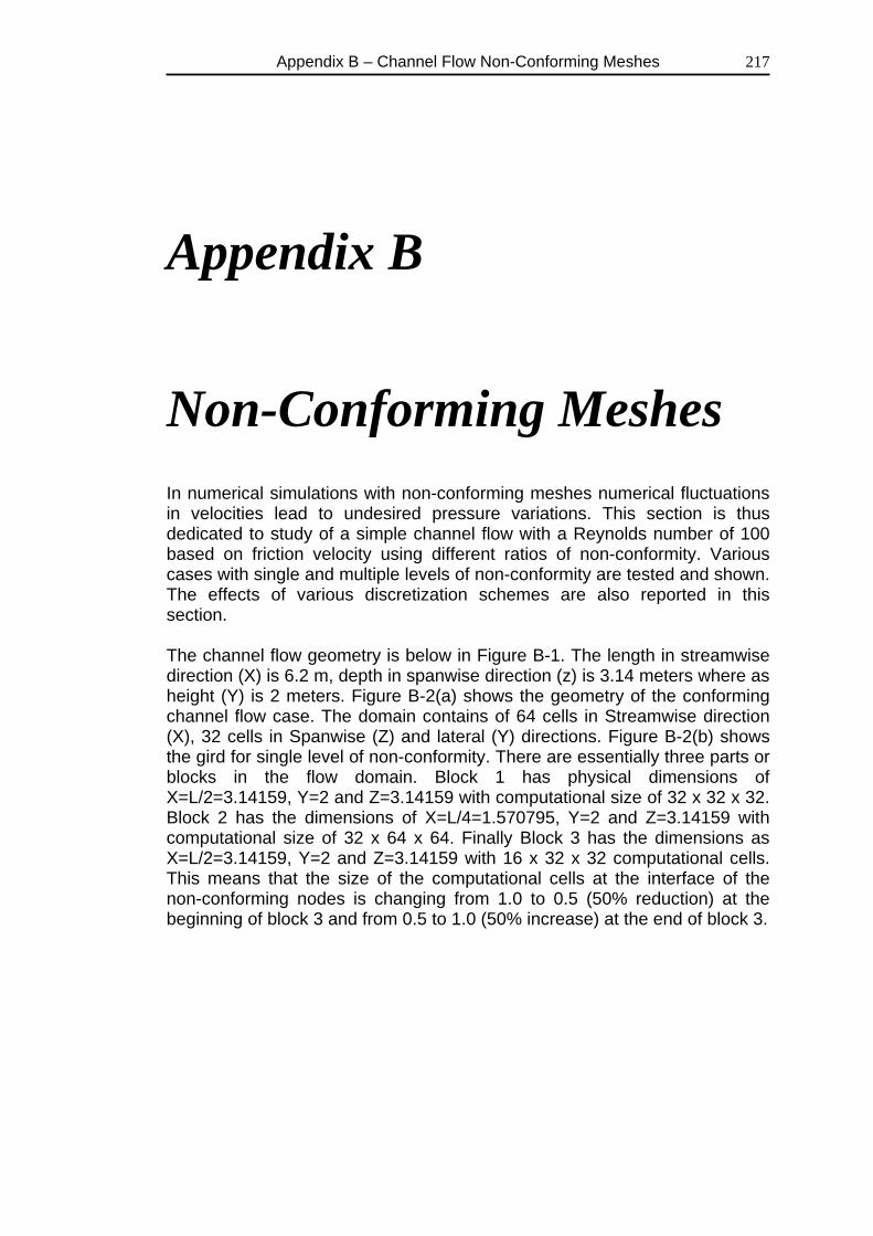
Appendix B – Channel Flow Non-Conforming Meshes
217
Appendix B Non-Conforming Meshes In numerical simulations with non-conforming meshes numerical fluctuations in velocities lead to undesired pressure variations. This section is thus dedicated to study of a simple channel flow with a Reynolds number of 100 based on friction velocity using different ratios of non-conformity. Various cases with single and multiple levels of non-conformity are tested and shown. The effects of various discretization schemes are also reported in this section. The channel flow geometry is below in Figure B-1. The length in streamwise direction (X) is 6.2 m, depth in spanwise direction (z) is 3.14 meters where as height (Y) is 2 meters. Figure B-2(a) shows the geometry of the conforming channel flow case. The domain contains of 64 cells in Streamwise direction (X), 32 cells in Spanwise (Z) and lateral (Y) directions. Figure B-2(b) shows the gird for single level of non-conformity. There are essentially three parts or blocks in the flow domain. Block 1 has physical dimensions of X=L/2=3.14159, Y=2 and Z=3.14159 with computational size of 32 x 32 x 32. Block 2 has the dimensions of X=L/4=1.570795, Y=2 and Z=3.14159 with computational size of 32 x 64 x 64. Finally Block 3 has the dimensions as X=L/2=3.14159, Y=2 and Z=3.14159 with 16 x 32 x 32 computational cells. This means that the size of the computational cells at the interface of the non-conforming nodes is changing from 1.0 to 0.5 (50% reduction) at the beginning of block 3 and from 0.5 to 1.0 (50% increase) at the end of block 3.
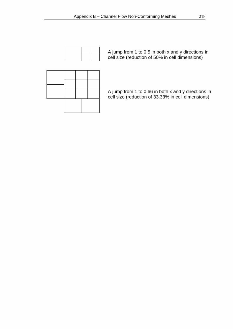
Appendix B – Channel Flow Non-Conforming Meshes
218
A jump from 1 to 0.5 in both x and y directions in cell size (reduction of 50% in cell dimensions)
A jump from 1 to 0.66 in both x and y directions in cell size (reduction of 33.33% in cell dimensions)
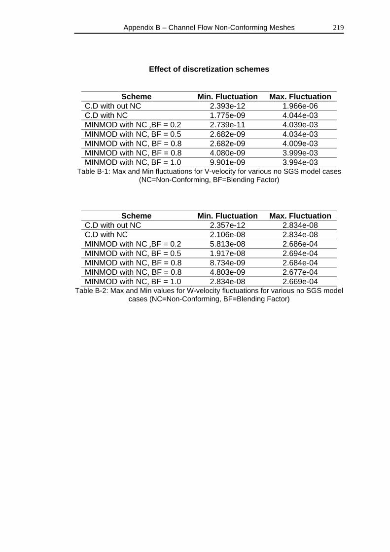
Appendix B – Channel Flow Non-Conforming Meshes
219
Effect of discretization schemes
Scheme Min. Fluctuation Max. Fluctuation C.D with out NC 2.393e-12 1.966e-06 C.D with NC 1.775e-09 4.044e-03 MINMOD with NC ,BF = 0.2 2.739e-11 4.039e-03 MINMOD with NC, BF = 0.5 2.682e-09 4.034e-03 MINMOD with NC, BF = 0.8 2.682e-09 4.009e-03 MINMOD with NC, BF = 0.8 4.080e-09 3.999e-03 MINMOD with NC, BF = 1.0 9.901e-09 3.994e-03
Table B-1: Max and Min fluctuations for V-velocity for various no SGS model cases (NC=Non-Conforming, BF=Blending Factor)
Scheme Min. Fluctuation Max. Fluctuation C.D with out NC 2.357e-12 2.834e-08 C.D with NC 2.106e-08 2.834e-08 MINMOD with NC ,BF = 0.2 5.813e-08 2.686e-04 MINMOD with NC, BF = 0.5 1.917e-08 2.694e-04 MINMOD with NC, BF = 0.8 8.734e-09 2.684e-04 MINMOD with NC, BF = 0.8 4.803e-09 2.677e-04 MINMOD with NC, BF = 1.0 2.834e-08 2.669e-04
Table B-2: Max and Min values for W-velocity fluctuations for various no SGS model cases (NC=Non-Conforming, BF=Blending Factor)
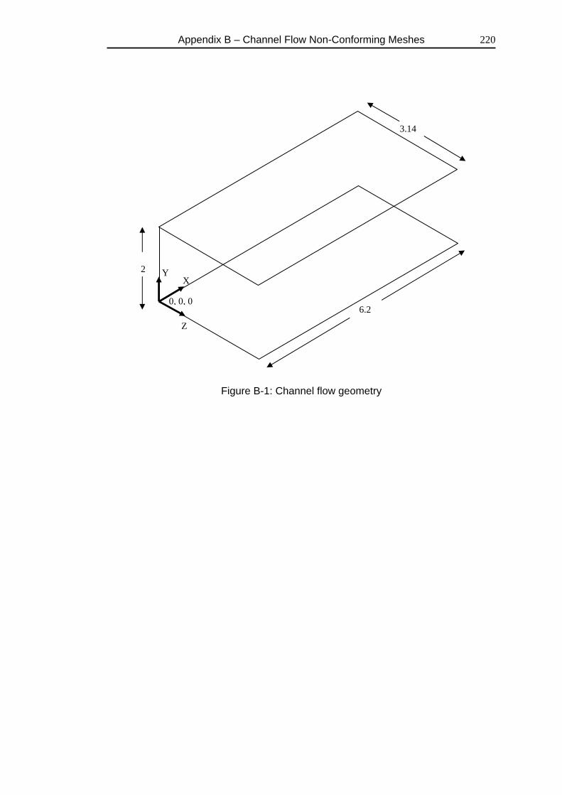
Appendix B – Channel Flow Non-Conforming Meshes
220
0, 0, 0
2
6.2
3.14
Z
X Y
Figure B-1: Channel flow geometry
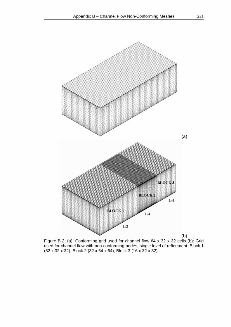
Appendix B – Channel Flow Non-Conforming Meshes
221
(a)
(b) Figure B-2: (a): Conforming grid used for channel flow 64 x 32 x 32 cells (b): Grid used for channel flow with non-conforming nodes, single level of refinement. Block 1 (32 x 32 x 32), Block 2 (32 x 64 x 64), Block 3 (16 x 32 x 32)
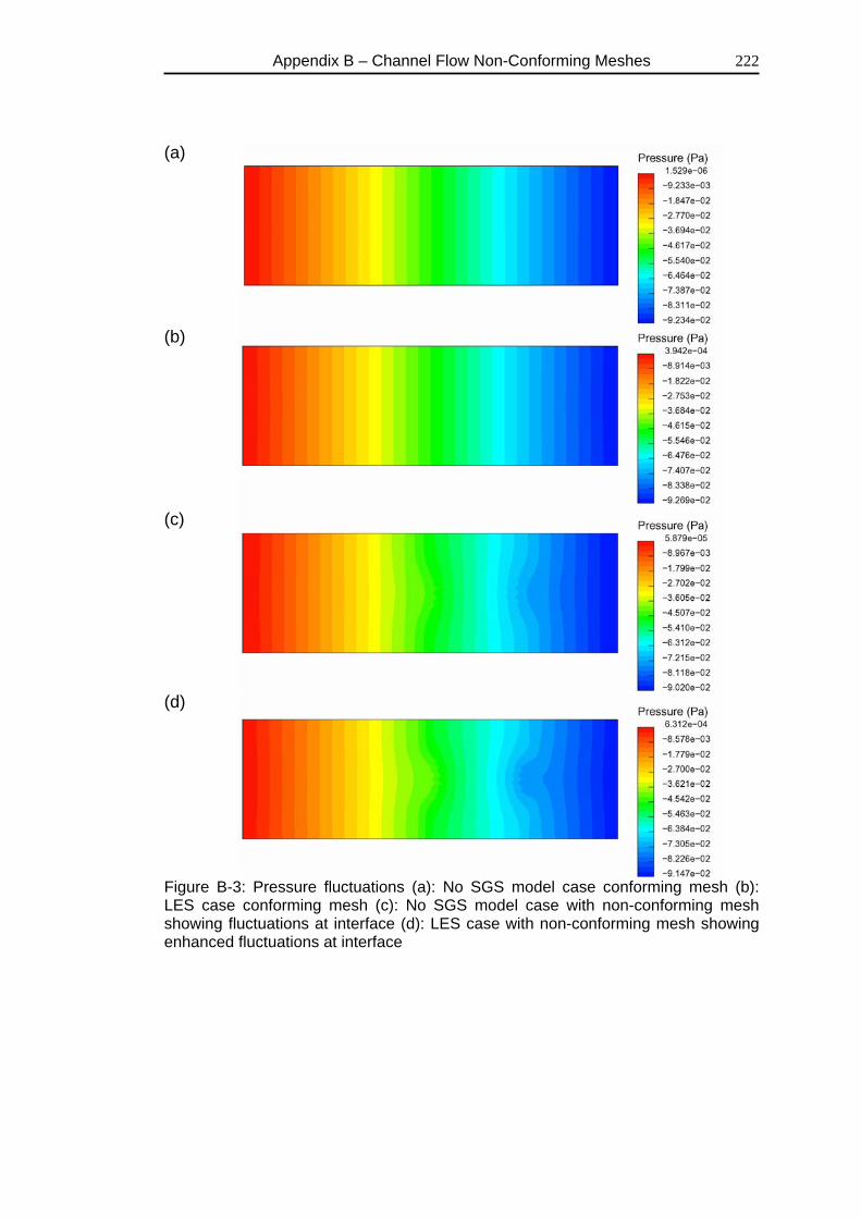
Appendix B – Channel Flow Non-Conforming Meshes
222
(a)
(b)
(c)
(d)
Figure B-3: Pressure fluctuations (a): No SGS model case conforming mesh (b): LES case conforming mesh (c): No SGS model case with non-conforming mesh showing fluctuations at interface (d): LES case with non-conforming mesh showing enhanced fluctuations at interface
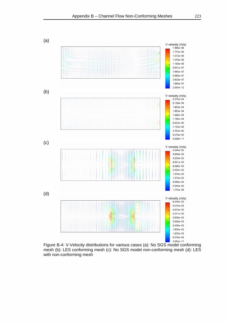
Appendix B – Channel Flow Non-Conforming Meshes
223
(a)
(b)
(c)
(d)
Figure B-4: V-Velocity distributions for various cases (a): No SGS model conforming mesh (b): LES conforming mesh (c): No SGS model non-conforming mesh (d): LES with non-conforming mesh
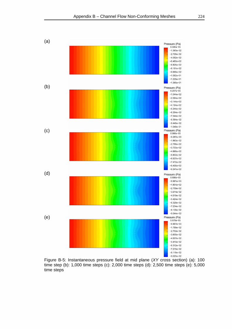
Appendix B – Channel Flow Non-Conforming Meshes
224
(a)
(b)
(c)
(d)
(e)
Figure B-5: Instantaneous pressure field at mid plane (XY cross section) (a): 100 time step (b): 1,000 time steps (c): 2,000 time steps (d): 2,500 time steps (e): 5,000 time steps
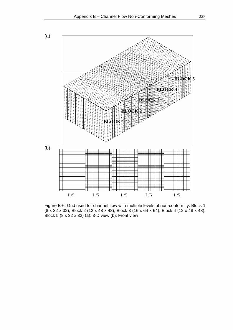
Appendix B – Channel Flow Non-Conforming Meshes
225
BLOCK 3
BLOCK 1
BLOCK 2
BLOCK 4
BLOCK 5
L/5 L/5 L/5 L/5 L/5
(a)
(b)
Figure B-6: Grid used for channel flow with multiple levels of non-conformity. Block 1 (8 x 32 x 32), Block 2 (12 x 48 x 48), Block 3 (16 x 64 x 64), Block 4 (12 x 48 x 48), Block 5 (8 x 32 x 32) (a): 3-D view (b): Front view
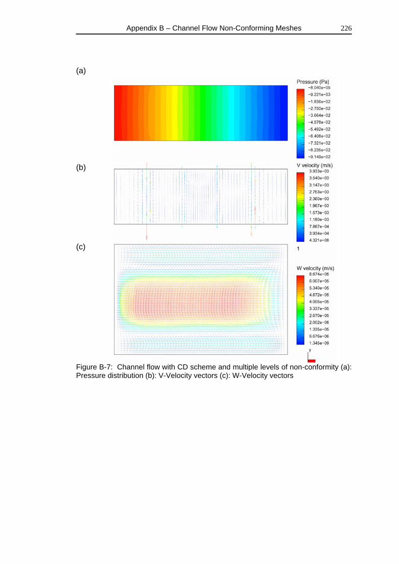
Appendix B – Channel Flow Non-Conforming Meshes
226
(a)
(b)
(c)
Figure B-7: Channel flow with CD scheme and multiple levels of non-conformity (a): Pressure distribution (b): V-Velocity vectors (c): W-Velocity vectors
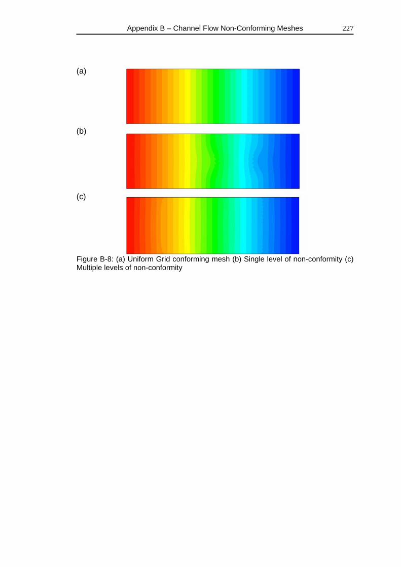
Appendix B – Channel Flow Non-Conforming Meshes
227
(a)
(b)
(c)
Figure B-8: (a) Uniform Grid conforming mesh (b) Single level of non-conformity (c) Multiple levels of non-conformity
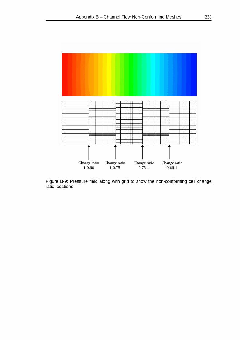
Appendix B – Channel Flow Non-Conforming Meshes
228
Change ratio 1-0.66
Change ratio 1-0.75
Change ratio 0.75-1
Change ratio 0.66-1
Figure B-9: Pressure field along with grid to show the non-conforming cell change ratio locations
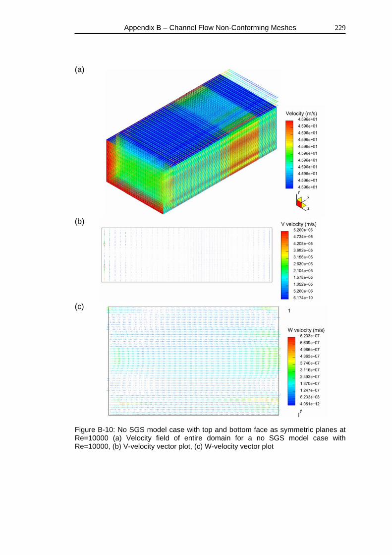
Appendix B – Channel Flow Non-Conforming Meshes
229
(a)
(b)
(c)
Figure B-10: No SGS model case with top and bottom face as symmetric planes at Re=10000 (a) Velocity field of entire domain for a no SGS model case with Re=10000, (b) V-velocity vector plot, (c) W-velocity vector plot
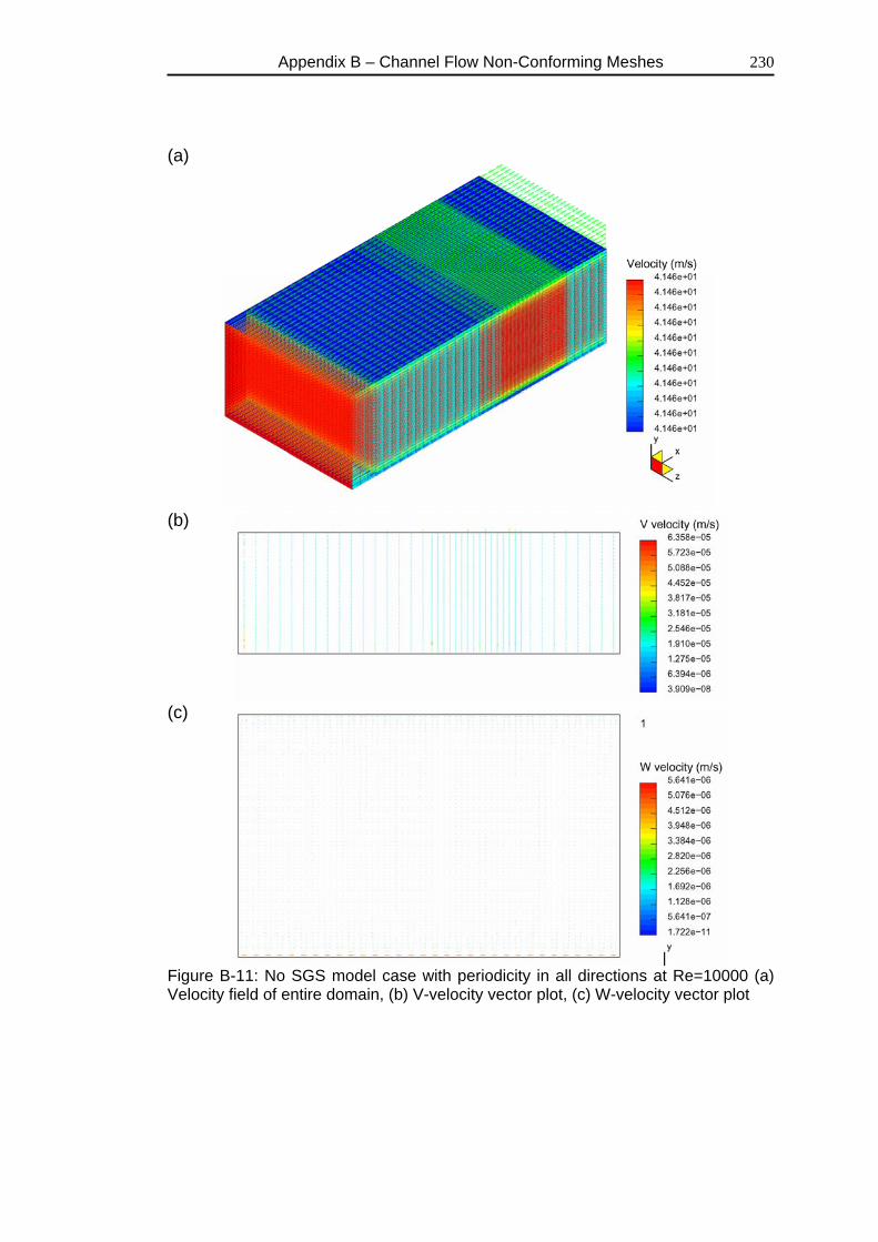
Appendix B – Channel Flow Non-Conforming Meshes
230
(a)
(b)
(c)
Figure B-11: No SGS model case with periodicity in all directions at Re=10000 (a) Velocity field of entire domain, (b) V-velocity vector plot, (c) W-velocity vector plot
Appendix B – Channel Flow Non-Conforming Meshes
231
Figure B-12: No SGS model case with no-slip at top face and symmetric boundary at the bottom face at Re=100 (a) Pressure plot, (b) V-velocity vector plot, (c) W-velocity vector plot
Appendix C – User Coding
232
Appendix C
User Coding This section contains FORTRAN subroutines for the collection of statistics for LES and URANS. These are followed by some additional subroutines to couple the user coding to the solvers post processor. In the end the reader will find subroutines for Van Driest wall damping function and Y+ calculation.
Appendix C – User Coding
233
Statistics for LES
( )
1
2
1 or alternatively
ii in
ii
i
ii i
ii i i
ni i
i ii i i i i ii
U U uUUn
u U U
u u U U
u uu u u u U U U Un
=
=
′= +
=
′ = −
′ ′ = −
′ ′′ ′ ′ ′= = −
∑
∑
Statistics for URANS
1
Resolved Modelled
Resolved
Modelled 1
ni
ii
i i i i i i
i ii i i i
ni i
i ii
UU
n
u u u u u u
u u U U U U
u uu u
n
=
=
=
′ ′ ′ ′ ′ ′= +
′ ′ = −
′ ′′ ′ =
∑
∑
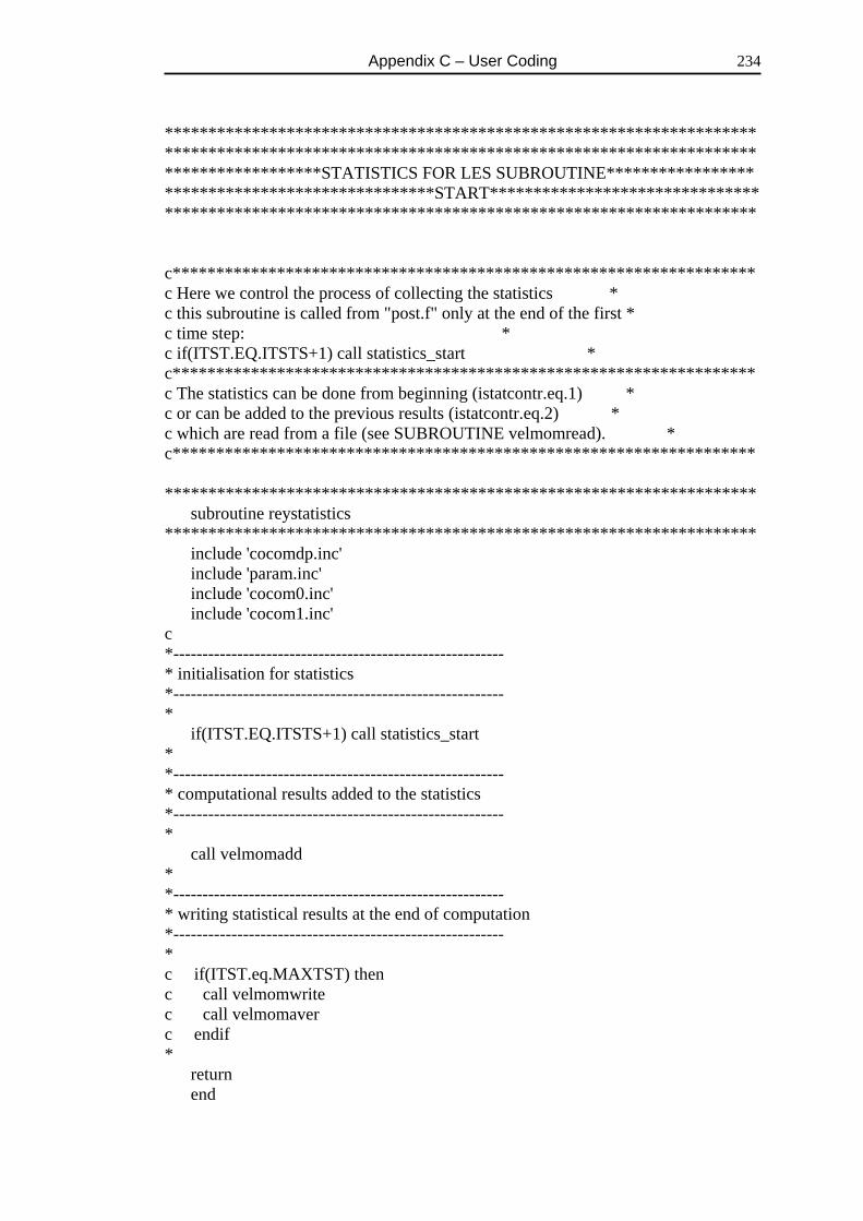
Appendix C – User Coding
234
******************************************************************** ******************************************************************** ******************STATISTICS FOR LES SUBROUTINE***************** *******************************START******************************* ******************************************************************** c******************************************************************* c Here we control the process of collecting the statistics * c this subroutine is called from "post.f" only at the end of the first * c time step: * c if(ITST.EQ.ITSTS+1) call statistics_start * c******************************************************************* c The statistics can be done from beginning (istatcontr.eq.1) * c or can be added to the previous results (istatcontr.eq.2) * c which are read from a file (see SUBROUTINE velmomread). * c******************************************************************* ******************************************************************** subroutine reystatistics ******************************************************************** include 'cocomdp.inc' include 'param.inc' include 'cocom0.inc' include 'cocom1.inc' c *--------------------------------------------------------- * initialisation for statistics *--------------------------------------------------------- * if(ITST.EQ.ITSTS+1) call statistics_start * *--------------------------------------------------------- * computational results added to the statistics *--------------------------------------------------------- * call velmomadd * *--------------------------------------------------------- * writing statistical results at the end of computation *--------------------------------------------------------- * c if(ITST.eq.MAXTST) then c call velmomwrite c call velmomaver c endif * return end
Appendix C – User Coding
235
******************************************************************** subroutine statistics_start ******************************************************************** include 'cocomdp.inc' include 'param.inc' include 'cocom0.inc' include 'cocom1.inc' c character fileime*100 logical lexist * *--------------------------------------------------------- * reading control parameter *--------------------------------------------------------- * if(nscrn.eq.1) write(*,*) ' initialisation for statistics ' fileime=probna(1:npro)//'/statistics_control' inquire(file=fileime,exist=lexist) * if(ITST.EQ.ITSTS+1) then if(lexist) then open(unit=31,file=fileime,status='unknown') read(31,*) istatcontr close(31) else write(*,'("STATISTICS: File : ",a30," is missing!")') & fileime write(*,'("STATISTICS: Program is stopped!")') STOP end if if(istatcontr.ne.1.AND.istatcontr.ne.2) then write(*,'(a)') & 'STATISTICS: Input file contains wrong parameters.', & 'It should be 1 or 2.' STOP end if end if *--------------------------------------------------------- * initialisation for statistics *--------------------------------------------------------- * if(istatcontr.eq.1) call velmominit *--------------------------------------------------------- * reading previous results for statistics *--------------------------------------------------------- * if(istatcontr.eq.2) call velmomread * return
Appendix C – User Coding
236
end ******************************************************************** subroutine velmominit ******************************************************************** include 'cocomdp.inc' include 'param.inc' include 'cocom0.inc' include 'cocom1.inc' *....................................................................... common/myvelmom1/ summtimes, & summu(3,nd02),summub(3,nd03), & summuu(3,3,nd02),summuub(3,3,nd03), & summp(nd02),summpb(nd03) *....................................................................... *--------------------------------------------------------- * Setting the cumulative velocity moments to zero *--------------------------------------------------------- * if(nscrn.eq.1) write(*,101) 101 format('STATISTICS: setting cumulative velocity moments to zero.') * summtimes=0. do mat=1,nmat do i=nsp(mat),nep(mat) do l=1,3 summu(l,i)=0. end do do l=1,3 do m=1,3 summuu(l,m,i)=0. end do end do summp(i)=0. end do * do ir=0,nreg do k=nsr(ir),ner(ir) do l=1,3 summub(l,k)=0. end do do l=1,3 do m=1,3 summuub(l,m,k)=0. end do end do summpb(k)=0. end do end do end do
Appendix C – User Coding
237
* return end ******************************************************************** subroutine velmomwrite ******************************************************************** include 'cocomdp.inc' include 'param.inc' include 'cocom0.inc' include 'cocom1.inc' *....................................................................... common/myvelmom1/ summtimes, & summu(3,nd02),summub(3,nd03), & summuu(3,3,nd02),summuub(3,3,nd03), & summp(nd02),summpb(nd03) character filen*100 character*6 ndfc *....................................................................... *--------------------------------------------------------- * Writting the cumulative velocity moments into a file *--------------------------------------------------------- * write(ndfc,'(i6.6)') itst write(*,*) ndfc c filen=probna(1:npro)//'/stat'//ndfc//'.res' lfd=npro+15 call filext(filen,lfd) open(32,file=filen(1:lfd),form='unformatted',status='unknown') * if(nscrn.eq.1) write(*,101) filen 101 format('STATISTICS: writing cumulative velocity moments into: ', & a100) * write(32) summtimes, & ((summu(l,ij),ij=1,nd02),l=1,3), & ((summub(l,ij),ij=1,nd03),l=1,3), & (((summuu(l,m,ij),ij=1,nd02),m=1,3),l=1,3), & (((summuub(l,m,ij),ij=1,nd03),m=1,3),l=1,3), & (summp(ij),ij=1,nd02),(summpb(ij),ij=1,nd03) close(32) * return end ******************************************************************** subroutine velmomadd ******************************************************************** include 'cocomdp.inc' include 'param.inc'
Appendix C – User Coding
238
include 'cocom0.inc' include 'cocom1.inc' *....................................................................... common/myvelmom1/ summtimes, & summu(3,nd02),summub(3,nd03), & summuu(3,3,nd02),summuub(3,3,nd03), & summp(nd02),summpb(nd03) *....................................................................... *--------------------------------------------------------- * Adding a set aof results to the statistics. *--------------------------------------------------------- * summtimes=summtimes+1. if(nscrn.eq.1) write(*,101) summtimes 101 format('STATISTICS: adding data set #',f6.0, & ' for computation of velocity moments ') * do mat=1,nmat do i=nsp(mat),nep(mat) do l=1,3 summu(l,i)=summu(l,i)+u(l,i) end do do l=1,3 do m=1,3 summuu(l,m,i)=summuu(l,m,i)+u(l,i)*u(m,i) end do end do summp(i)=summp(i)+p(i) end do * do ir=0,nreg do k=nsr(ir),ner(ir) do l=1,3 summub(l,k)=summub(l,k)+ub(l,k) end do do l=1,3 do m=1,3 summuub(l,m,k)=summuub(l,m,k)+ub(l,k)*ub(m,k) end do end do summpb(k)=summpb(k)+pb(k) end do end do end do * return end ******************************************************************** subroutine velmomread
Appendix C – User Coding
239
******************************************************************** include 'cocomdp.inc' include 'param.inc' include 'cocom0.inc' include 'cocom1.inc' *....................................................................... common/myvelmom1/ summtimes, & summu(3,nd02),summub(3,nd03), & summuu(3,3,nd02),summuub(3,3,nd03), & summp(nd02),summpb(nd03) character filen*100 *....................................................................... *--------------------------------------------------------- * Reading the cumulative velocity moments from a file *--------------------------------------------------------- * filen=probna(1:npro)//'/statistics.res' lfd=npro+15 call filext(filen,lfd) open(32,file=filen(1:lfd),form='unformatted',status='unknown') * if(nscrn.eq.1) write(*,101) filen 101 format('STATISTICS: reading velocity moments from file ',a20) * read (32) summtimes, & ((summu(l,ij),ij=1,nd02),l=1,3), & ((summub(l,ij),ij=1,nd03),l=1,3), & (((summuu(l,m,ij),ij=1,nd02),m=1,3),l=1,3), & (((summuub(l,m,ij),ij=1,nd03),m=1,3),l=1,3), & (summp(ij),ij=1,nd02),(summpb(ij),ij=1,nd03) if(nscrn.eq.1) write(*,102) summtimes 102 format('STATISTICS: There are ',f10.0,' data sets collected.') close(32) * return end ******************************************************************** subroutine velmomaver ******************************************************************** include 'cocomdp.inc' include 'param.inc' include 'cocom0.inc' include 'cocom1.inc' *....................................................................... common/myvelmom1/ summtimes, & summu(3,nd02),summub(3,nd03), & summuu(3,3,nd02),summuub(3,3,nd03), & summp(nd02),summpb(nd03) common/mysumvel2/ averu(3,nd02),averub(3,nd03),
Appendix C – User Coding
240
& averuu(3,3,nd02),averuub(3,3,nd03), & averp(nd02),averpb(nd03) *....................................................................... integer ikeyword(10) character keyword*10 *....................................................................... *--------------------------------------------------------- * Averaging the data before printing for postprocessing *--------------------------------------------------------- * if(nscrn.eq.1) write(*,101) summtimes 101 format('STATISTICS: averaging collected data of ',f6.0,' samples', & ', just before printing for postprocessing.') * do mat=1,nmat do i=nsp(mat),nep(mat) do l=1,3 averu(l,i)=summu(l,i)/summtimes end do do l=1,3 do m=1,3 averuu(l,m,i)=summuu(l,m,i)/summtimes end do end do averp(i)=summp(i)/summtimes end do * do ir=0,nreg do k=nsr(ir),ner(ir) do l=1,3 averub(l,k)=summub(l,k)/summtimes end do do l=1,3 do m=1,3 averuub(l,m,k)=summuub(l,m,k)/summtimes end do end do averpb(k)=summpb(k)/summtimes end do end do end do *....................................................................... *....................................................................... do mat=1,nmat do i=nsp(mat),nep(mat) do l=1,3 do m=1,3 averuu(l,m,i)=averuu(l,m,i)-averu(l,i)*averu(m,i) end do
Appendix C – User Coding
241
end do end do * do ir=0,nreg do k=nsr(ir),ner(ir) do l=1,3 do m=1,3 averuub(l,m,k)=averuub(l,m,k)-averub(l,k)*averub(m,k) end do end do end do end do end do *....................................................................... return end ******************************************************************** subroutine velmomaver_z ******************************************************************** include 'cocomdp.inc' include 'param.inc' include 'cocom0.inc' include 'cocom1.inc' *....................................................................... common/mysumvel2/ averu(3,nd02),averub(3,nd03), & averuu(3,3,nd02),averuub(3,3,nd03), & averp(nd02),averpb(nd03) common/mysumvel3/ averuzz(3,nd02), averuuzz(3,3,nd02), $ averpzz(nd02), averubzz(3,nd03), $ averuubzz(3,3,nd03), averpbzz(nd03) *....................................................................... integer ikeyword(10) character keyword*10 *....................................................................... real xface(nd02) real yface(nd02) real zface(nd02) c real xfaceb(nd02) real yfaceb(nd02) real zfaceb(nd02) c real averuz(3,nd02), averuuz(3,3,nd02), $ averpz(nd02) real averubz(3,nd02), averuubz(3,3,nd02), $ averpbz(nd02) *--------------------------------------------------------- * Averaging the data before printing for postprocessing *---------------------------------------------------------
Appendix C – User Coding
242
* zzmmiinn=5.7e-2 c nbzzi=0 do mat=1,nmat do i=nsp(mat),nep(mat) if (xp(3,i).le.zzmmiinn.and.xp(3,i).ge.0.) then nbzzi=nbzzi+1 c write(*,*) xp(3,i),zzmmiinn xface(nbzzi)=xp(1,i) yface(nbzzi)=xp(2,i) zface(nbzzi)=xp(3,i) endif enddo enddo c c Inner domain c do mat=1,nmat do k=1,nbzzi navz=0 do l=1,3 averuz(l,k)=0. do m=1,3 averuuz(l,m,k)=0. enddo enddo averpz(k)=0. do i=nsp(mat),nep(mat) xdifxp=xface(k)-xp(1,i) ydifxp=yface(k)-xp(2,i) if (abs(xdifxp).le.1.e-5 $ .and.abs(ydifxp).le.1.e-5) then do l=1,3 averuz(l,k)=averuz(l,k)+averu(l,i) do m=1,3 averuuz(l,m,k)=averuuz(l,m,k)+averuu(l,m,i) enddo enddo averpz(k)=averpz(k)+averp(i) navz=navz+1 endif enddo do l=1,3 averuz(l,k)=averuz(l,k)/float(navz) do m=1,3 averuuz(l,m,k)=averuuz(l,m,k)/float(navz) enddo enddo
Appendix C – User Coding
243
averpz(k)=averpz(k)/float(navz) enddo enddo c do mat=1,nmat do k=1,nbzzi do i=nsp(mat),nep(mat) xdifxp=xface(k)-xp(1,i) ydifxp=yface(k)-xp(2,i) if (abs(xdifxp).le.1.e-5 $ .and.abs(ydifxp).le.1.e-5) then do l=1,3 averuzz(l,i)=averuz(l,k) do m=1,3 averuuzz(l,m,i)=averuuz(l,m,k) enddo enddo averpzz(i)=averpz(k) endif enddo enddo enddo c c Boundaries c nbzzib=0 do ir=0,nreg do i=nsr(ir),ner(ir) if (xb(3,i).le.zzmmiinn.and.xb(3,i).ge.0.) then nbzzib=nbzzib+1 xfaceb(nbzzib)=xb(1,i) yfaceb(nbzzib)=xb(2,i) zfaceb(nbzzib)=xb(3,i) endif enddo enddo c write(*,*) 'nbzzi ',nbzzi write(*,*) 'nbzzib ',nbzzib c do ir=0,nreg do k=1,nbzzib navzb=0 do l=1,3 averubz(l,k)=0. do m=1,3 averuubz(l,m,k)=0. enddo enddo
Appendix C – User Coding
244
averpbz(k)=0. do i=nsr(ir),ner(ir) xdifxp=xfaceb(k)-xb(1,i) ydifxp=yfaceb(k)-xb(2,i) if (abs(xdifxp).le.1.e-5 $ .and.abs(ydifxp).le.1.e-5) then do l=1,3 averubz(l,k)=averubz(l,k)+averub(l,i) do m=1,3 averuubz(l,m,k)=averuubz(l,m,k)+averuub(l,m,i) enddo enddo averpbz(k)=averpbz(k)+averpb(i) navzb=navzb+1 endif enddo if (navzb.ne.0) then do l=1,3 averubz(l,k)=averubz(l,k)/float(navzb) do m=1,3 averuubz(l,m,k)=averuubz(l,m,k)/float(navzb) enddo enddo averpbz(k)=averpbz(k)/float(navzb) endif enddo enddo c do ir=0,nreg do k=1,nbzzib do i=nsr(ir),ner(ir) xdifxp=xfaceb(k)-xb(1,i) ydifxp=yfaceb(k)-xb(2,i) if (abs(xdifxp).le.1.e-5 $ .and.abs(ydifxp).le.1.e-5) then do l=1,3 averubzz(l,i)=averubz(l,k) do m=1,3 averuubzz(l,m,i)=averuubz(l,m,k) enddo enddo averpbzz(i)=averpbz(k) endif enddo enddo enddo c return end

Appendix C – User Coding
245
******************************************************************** ******************************************************************** ******************STATISTICS FOR LES SUBROUTINE***************** *********************************END******************************* ********************************************************************

Appendix C – User Coding
246
******************************************************************** ******************************************************************** *****************STATISTICS FOR URANS SUBROUTINE*************** *******************************START******************************* ******************************************************************** c******************************************************************* c Here we control the process of collecting the statistics * c this subroutine is called from "post.f" only at the end of the first * c time step: * c if(ITST.EQ.ITSTS+1) call statistics_start * c******************************************************************* c The statistics can be done from beginning (istatcontr.eq.1) * c or can be added to the previous results (istatcontr.eq.2) * c which are read from a file (see SUBROUTINE velmomread). * c******************************************************************* ******************************************************************** subroutine reystatistics ******************************************************************** include 'cocomdp.inc' include 'param.inc' include 'cocom0.inc' include 'cocom1.inc' c *--------------------------------------------------------- * initialisation for statistics *--------------------------------------------------------- * if(ITST.EQ.ITSTS+1) call statistics_start * *--------------------------------------------------------- * computational results added to the statistics *--------------------------------------------------------- * call velmomadd * *--------------------------------------------------------- * writing statistical results at the end of computation *--------------------------------------------------------- * c if(ITST.eq.MAXTST) then c call velmomwrite c call velmomaver c endif * return
Appendix C – User Coding
247
end ******************************************************************** subroutine statistics_start ******************************************************************** include 'cocomdp.inc' include 'param.inc' include 'cocom0.inc' include 'cocom1.inc' c character fileime*100 logical lexist * *--------------------------------------------------------- * reading control parameter *--------------------------------------------------------- * if(nscrn.eq.1) write(*,*) ' initialisation for statistics ' fileime=probna(1:npro)//'/statistics_control' inquire(file=fileime,exist=lexist) * if(ITST.EQ.ITSTS+1) then if(lexist) then open(unit=31,file=fileime,status='unknown') read(31,*) istatcontr close(31) else write(*,'("STATISTICS: File : ",a30," is missing!")') & fileime write(*,'("STATISTICS: Program is stopped!")') STOP end if if(istatcontr.ne.1.AND.istatcontr.ne.2) then write(*,'(a)') & 'STATISTICS: Input file contains wrong parameters.', & 'It should be 1 or 2.' STOP end if end if *--------------------------------------------------------- * initialisation for statistics *--------------------------------------------------------- * if(istatcontr.eq.1) call velmominit *--------------------------------------------------------- * reading previous results for statistics *--------------------------------------------------------- * if(istatcontr.eq.2) call velmomread *
Appendix C – User Coding
248
return end ******************************************************************** subroutine velmominit ******************************************************************** include 'cocomdp.inc' include 'param.inc' include 'cocom0.inc' include 'cocom1.inc' *....................................................................... common/myvelmom1/ summtimes, & summu(3,nd02),summub(3,nd03), & summuu(3,3,nd02),summuub(3,3,nd03), & summp(nd02),summpb(nd03) *....................................................................... *--------------------------------------------------------- * Setting the cumulative velocity moments to zero *--------------------------------------------------------- * if(nscrn.eq.1) write(*,101) 101 format('STATISTICS: setting cumulative velocity moments to zero.') * summtimes=0. do mat=1,nmat do i=nsp(mat),nep(mat) do l=1,3 summu(l,i)=0. end do do l=1,3 do m=1,3 summuu(l,m,i)=0. end do end do summp(i)=0. end do * do ir=0,nreg do k=nsr(ir),ner(ir) do l=1,3 summub(l,k)=0. end do do l=1,3 do m=1,3 summuub(l,m,k)=0. end do end do summpb(k)=0. end do end do
Appendix C – User Coding
249
end do * return end ******************************************************************** subroutine velmomwrite ******************************************************************** include 'cocomdp.inc' include 'param.inc' include 'cocom0.inc' include 'cocom1.inc' *....................................................................... common/myvelmom1/ summtimes, & summu(3,nd02),summub(3,nd03), & summuu(3,3,nd02),summuub(3,3,nd03), & summp(nd02),summpb(nd03) character filen*100 character*6 ndfc *....................................................................... *--------------------------------------------------------- * Writting the cumulative velocity moments into a file *--------------------------------------------------------- * write(ndfc,'(i6.6)') itst write(*,*) ndfc c filen=probna(1:npro)//'/stat'//ndfc//'.res' lfd=npro+15 call filext(filen,lfd) open(32,file=filen(1:lfd),form='unformatted',status='unknown') * if(nscrn.eq.1) write(*,101) filen 101 format('STATISTICS: writing cumulative velocity moments into: ', & a100) * write(32) summtimes, & ((summu(l,ij),ij=1,nd02),l=1,3), & ((summub(l,ij),ij=1,nd03),l=1,3), & (((summuu(l,m,ij),ij=1,nd02),m=1,3),l=1,3), & (((summuub(l,m,ij),ij=1,nd03),m=1,3),l=1,3), & (summp(ij),ij=1,nd02),(summpb(ij),ij=1,nd03) close(32) * return end ******************************************************************** subroutine velmomadd ******************************************************************** include 'cocomdp.inc'
Appendix C – User Coding
250
include 'param.inc' include 'cocom0.inc' include 'cocom1.inc' *....................................................................... common/myvelmom1/ summtimes, & summu(3,nd02),summub(3,nd03), & summuu(3,3,nd02),summuub(3,3,nd03), & summp(nd02),summpb(nd03) real uuu(3,3,nd02),uuub(3,3,nd03) *....................................................................... *--------------------------------------------------------- * Adding a set aof results to the statistics. *--------------------------------------------------------- * summtimes=summtimes+1. if(nscrn.eq.1) write(*,101) summtimes 101 format('STATISTICS: adding data set #',f6.0, & ' for computation of velocity moments ') * do mat=1,nmat do i=nsp(mat),nep(mat) uuu(1,1,i)=uu(i) uuu(2,2,i)=vv(i) uuu(3,3,i)=ww(i) uuu(1,2,i)=uv(i) uuu(2,3,i)=vw(i) uuu(1,3,i)=uw(i) end do end do do mat=1,nmat do i=nsp(mat),nep(mat) do l=1,3 summu(l,i)=summu(l,i)+u(l,i) end do do l=1,3 do m=1,3 summuu(l,m,i)=summuu(l,m,i)+(u(l,i)*u(m,i))+uuu(l,m,i) end do end do summp(i)=summp(i)+p(i) end do * do ir=0,nreg do k=nsr(ir),ner(ir) uuub(1,1,k)=uu(k) uuub(2,2,k)=vv(k) uuub(3,3,k)=ww(k) uuub(1,2,k)=uv(k) uuub(2,3,k)=vw(k)
Appendix C – User Coding
251
uuub(1,3,k)=uw(k) end do end do do ir=0,nreg do k=nsr(ir),ner(ir) do l=1,3 summub(l,k)=summub(l,k)+ub(l,k) end do do l=1,3 do m=1,3 summuub(l,m,k)=summuub(l,m,k)+(ub(l,k)*ub(m,k)) & +uuub(l,m,k) end do end do summpb(k)=summpb(k)+pb(k) end do end do end do * return end ******************************************************************** subroutine velmomread ******************************************************************** include 'cocomdp.inc' include 'param.inc' include 'cocom0.inc' include 'cocom1.inc' *....................................................................... common/myvelmom1/ summtimes, & summu(3,nd02),summub(3,nd03), & summuu(3,3,nd02),summuub(3,3,nd03), & summp(nd02),summpb(nd03) character filen*100 *....................................................................... *--------------------------------------------------------- * Reading the cumulative velocity moments from a file *--------------------------------------------------------- * filen=probna(1:npro)//'/statistics.res' lfd=npro+15 call filext(filen,lfd) open(32,file=filen(1:lfd),form='unformatted',status='unknown') * if(nscrn.eq.1) write(*,101) filen 101 format('STATISTICS: reading velocity moments from file ',a20) * read (32) summtimes, & ((summu(l,ij),ij=1,nd02),l=1,3),
Appendix C – User Coding
252
& ((summub(l,ij),ij=1,nd03),l=1,3), & (((summuu(l,m,ij),ij=1,nd02),m=1,3),l=1,3), & (((summuub(l,m,ij),ij=1,nd03),m=1,3),l=1,3), & (summp(ij),ij=1,nd02),(summpb(ij),ij=1,nd03) if(nscrn.eq.1) write(*,102) summtimes 102 format('STATISTICS: There are ',f10.0,' data sets collected.') close(32) * return end ******************************************************************** subroutine velmomaver ******************************************************************** include 'cocomdp.inc' include 'param.inc' include 'cocom0.inc' include 'cocom1.inc' *....................................................................... common/myvelmom1/ summtimes, & summu(3,nd02),summub(3,nd03), & summuu(3,3,nd02),summuub(3,3,nd03), & summp(nd02),summpb(nd03) common/mysumvel2/ averu(3,nd02),averub(3,nd03), & averuu(3,3,nd02),averuub(3,3,nd03), & averp(nd02),averpb(nd03) *....................................................................... integer ikeyword(10) character keyword*10 *....................................................................... *--------------------------------------------------------- * Averaging the data before printing for postprocessing *--------------------------------------------------------- * if(nscrn.eq.1) write(*,101) summtimes 101 format('STATISTICS: averaging collected data of ',f6.0,' samples', & ', just before printing for postprocessing.') * do mat=1,nmat do i=nsp(mat),nep(mat) do l=1,3 averu(l,i)=summu(l,i)/summtimes end do do l=1,3 do m=1,3 averuu(l,m,i)=summuu(l,m,i)/summtimes end do end do averp(i)=summp(i)/summtimes end do
Appendix C – User Coding
253
* do ir=0,nreg do k=nsr(ir),ner(ir) do l=1,3 averub(l,k)=summub(l,k)/summtimes end do do l=1,3 do m=1,3 averuub(l,m,k)=summuub(l,m,k)/summtimes end do end do averpb(k)=summpb(k)/summtimes end do end do end do *....................................................................... *....................................................................... do mat=1,nmat do i=nsp(mat),nep(mat) do l=1,3 do m=1,3 averuu(l,m,i)=averuu(l,m,i)-averu(l,i)*averu(m,i) end do end do end do * do ir=0,nreg do k=nsr(ir),ner(ir) do l=1,3 do m=1,3 averuub(l,m,k)=averuub(l,m,k)-averub(l,k)*averub(m,k) end do end do end do end do end do *....................................................................... return end ******************************************************************** subroutine velmomaver_z ******************************************************************** include 'cocomdp.inc' include 'param.inc' include 'cocom0.inc' include 'cocom1.inc' *....................................................................... common/mysumvel2/ averu(3,nd02),averub(3,nd03), & averuu(3,3,nd02),averuub(3,3,nd03),
Appendix C – User Coding
254
& averp(nd02),averpb(nd03) common/mysumvel3/ averuzz(3,nd02), averuuzz(3,3,nd02), & averpzz(nd02), averubzz(3,nd03), & averuubzz(3,3,nd03), averpbzz(nd03) *....................................................................... integer ikeyword(10) character keyword*10 *....................................................................... real xface(nd02) real yface(nd02) real zface(nd02) c real xfaceb(nd02) real yfaceb(nd02) real zfaceb(nd02) c real averuz(3,nd02), averuuz(3,3,nd02), $ averpz(nd02) real averubz(3,nd02), averuubz(3,3,nd02), $ averpbz(nd02) *--------------------------------------------------------- * Averaging the data before printing for postprocessing *--------------------------------------------------------- * zzmmiinn=5.7e-2 c nbzzi=0 do mat=1,nmat do i=nsp(mat),nep(mat) if (xp(3,i).le.zzmmiinn.and.xp(3,i).ge.0.) then nbzzi=nbzzi+1 c write(*,*) xp(3,i),zzmmiinn xface(nbzzi)=xp(1,i) yface(nbzzi)=xp(2,i) zface(nbzzi)=xp(3,i) endif enddo enddo c c Inner domain c do mat=1,nmat do k=1,nbzzi navz=0 do l=1,3 averuz(l,k)=0. do m=1,3 averuuz(l,m,k)=0. enddo
Appendix C – User Coding
255
enddo averpz(k)=0. do i=nsp(mat),nep(mat) xdifxp=xface(k)-xp(1,i) ydifxp=yface(k)-xp(2,i) if (abs(xdifxp).le.1.e-5 $ .and.abs(ydifxp).le.1.e-5) then do l=1,3 averuz(l,k)=averuz(l,k)+averu(l,i) do m=1,3 averuuz(l,m,k)=averuuz(l,m,k)+averuu(l,m,i) enddo enddo averpz(k)=averpz(k)+averp(i) navz=navz+1 endif enddo do l=1,3 averuz(l,k)=averuz(l,k)/float(navz) do m=1,3 averuuz(l,m,k)=averuuz(l,m,k)/float(navz) enddo enddo averpz(k)=averpz(k)/float(navz) enddo enddo c do mat=1,nmat do k=1,nbzzi do i=nsp(mat),nep(mat) xdifxp=xface(k)-xp(1,i) ydifxp=yface(k)-xp(2,i) if (abs(xdifxp).le.1.e-5 $ .and.abs(ydifxp).le.1.e-5) then do l=1,3 averuzz(l,i)=averuz(l,k) do m=1,3 averuuzz(l,m,i)=averuuz(l,m,k) enddo enddo averpzz(i)=averpz(k) endif enddo enddo enddo c c Boundaries c nbzzib=0
Appendix C – User Coding
256
do ir=0,nreg do i=nsr(ir),ner(ir) if (xb(3,i).le.zzmmiinn.and.xb(3,i).ge.0.) then nbzzib=nbzzib+1 xfaceb(nbzzib)=xb(1,i) yfaceb(nbzzib)=xb(2,i) zfaceb(nbzzib)=xb(3,i) endif enddo enddo c write(*,*) 'nbzzi ',nbzzi write(*,*) 'nbzzib ',nbzzib c do ir=0,nreg do k=1,nbzzib navzb=0 do l=1,3 averubz(l,k)=0. do m=1,3 averuubz(l,m,k)=0. enddo enddo averpbz(k)=0. do i=nsr(ir),ner(ir) xdifxp=xfaceb(k)-xb(1,i) ydifxp=yfaceb(k)-xb(2,i) if (abs(xdifxp).le.1.e-5 $ .and.abs(ydifxp).le.1.e-5) then do l=1,3 averubz(l,k)=averubz(l,k)+averub(l,i) do m=1,3 averuubz(l,m,k)=averuubz(l,m,k)+averuub(l,m,i) enddo enddo averpbz(k)=averpbz(k)+averpb(i) navzb=navzb+1 endif enddo if (navzb.ne.0) then do l=1,3 averubz(l,k)=averubz(l,k)/float(navzb) do m=1,3 averuubz(l,m,k)=averuubz(l,m,k)/float(navzb) enddo enddo averpbz(k)=averpbz(k)/float(navzb) endif enddo
Appendix C – User Coding
257
enddo c do ir=0,nreg do k=1,nbzzib do i=nsr(ir),ner(ir) xdifxp=xfaceb(k)-xb(1,i) ydifxp=yfaceb(k)-xb(2,i) if (abs(xdifxp).le.1.e-5 $ .and.abs(ydifxp).le.1.e-5) then do l=1,3 averubzz(l,i)=averubz(l,k) do m=1,3 averuubzz(l,m,i)=averuubz(l,m,k) enddo enddo averpbzz(i)=averpbz(k) endif enddo enddo enddo c return end ******************************************************************** ******************************************************************** *****************STATISTICS FOR URANS SUBROUTINE*************** *******************************END********************************* ********************************************************************
Appendix C – User Coding
258
******************************************************************** ******************************************************************** **************** COUPLING USER CODING SUBROUTINE************** ******************************START******************************** ******************************************************************** c******************************************************************* subroutine addud(iwmode) c******************************************************************* c Add user data for post-processing. Each data set has to be marked c with a unique keyword which has one of the values: UD01, UD02, c ..., UD99. The data can be later loaded into Cometpp using the c STLO command, e.g. c c STLO 4 UD02 c c IWMODE defines if the data is to be added to restart file c (IWMODE=2) or to the file wich contains the data of the current c time step (IWMODE=1) c----------------------------------------------------------------------- include 'cocomdp.inc' include 'param.inc' include 'cocom0.inc' include 'cocom1.inc' *....................................................................... common/myvelmom1/ summtimes, & summu(3,nd02),summub(3,nd03), & summuu(3,3,nd02),summuub(3,3,nd03), & summp(nd02),summpb(nd03) common/mysumvel2/ averu(3,nd02),averub(3,nd03), & averuu(3,3,nd02),averuub(3,3,nd03), & averp(nd02),averpb(nd03) common/mysumvel3/ averuzz(3,nd02), averuuzz(3,3,nd02), $ averpzz(nd02), averubzz(3,nd03), $ averuubzz(3,3,nd03), averpbzz(nd03) real umoycel, uumoycel, ekcel, eecel, dudycel common/vvortt3/ umoycel(3,nd03), uumoycel(3,nd03), $ ekcel(nd03), eecel(nd03), dudycel(3,nd03) c *....................................................................... integer ikeyword(10) character keyword*10 character*20 filen *....................................................................... * *--------------------------------------------------------- * writing statistical results at the end of computation *---------------------------------------------------------
Appendix C – User Coding
259
* call velmomaver * call velmomaver_z *....................................................................... 101 format('STATISTICS: appending data for: ',a4) 102 format('STATISTICS: appending data for postprocessing!') if(nscrn.eq.1) write(*,102) do l=1,3 keyword='UD00' write(keyword(4:4),'(i1)') l do i=1,4 ikeyword(i)=ichar(keyword(i:i)) end do do ij=1,nd02 pp(ij)=averu(l,ij) end do do ij=1,nd03 ppb(ij)=averub(l,ij) end do c if(nscrn.eq.1) write(*,101) keyword call appendfi(pp,ppb,ikeyword,4,iwmode) end do *....................................................................... do l=1,3 do m=1,3 keyword='UD00' write(keyword(3:3),'(i1)') l write(keyword(4:4),'(i1)') m do i=1,4 ikeyword(i)=ichar(keyword(i:i)) end do do ij=1,nd02 pp(ij)=averuu(l,m,ij) end do do ij=1,nd03 ppb(ij)=averuub(l,m,ij) end do c if(nscrn.eq.1) write(*,101) keyword call appendfi(pp,ppb,ikeyword,4,iwmode) end do end do *....................................................................... do l=1,3 keyword='UD50' write(keyword(4:4),'(i1)') l do i=1,4 ikeyword(i)=ichar(keyword(i:i)) end do do ij=1,nd02
Appendix C – User Coding
260
pp(ij)=averuzz(l,ij) end do do ij=1,nd03 ppb(ij)=averubzz(l,ij) end do c if(nscrn.eq.1) write(*,101) keyword call appendfi(pp,ppb,ikeyword,4,iwmode) end do *....................................................................... do l=1,3 do m=1,3 keyword='UD00' write(keyword(3:3),'(i1)') l+5 write(keyword(4:4),'(i1)') m do i=1,4 ikeyword(i)=ichar(keyword(i:i)) end do do ij=1,nd02 pp(ij)=averuuzz(l,m,ij) end do do ij=1,nd03 ppb(ij)=averuubzz(l,m,ij) end do c if(nscrn.eq.1) write(*,101) keyword call appendfi(pp,ppb,ikeyword,4,iwmode) end do end do *....................................................................... keyword='UD04' do i=1,4 ikeyword(i)=ichar(keyword(i:i)) end do do ij=1,nd02 pp(ij)=averp(ij) end do do ij=1,nd03 ppb(ij)=averpb(ij) end do c if(nscrn.eq.1) write(*,101) keyword call appendfi(pp,ppb,ikeyword,4,iwmode) *....................................................................... keyword='UD54' do i=1,4 ikeyword(i)=ichar(keyword(i:i)) end do do ij=1,nd02 pp(ij)=averpzz(ij) end do do ij=1,nd03

Appendix C – User Coding
261
ppb(ij)=averpbzz(ij) end do c if(nscrn.eq.1) write(*,101) keyword call appendfi(pp,ppb,ikeyword,4,iwmode) c*....................................................................... call velmomwrite return end ******************************************************************** ******************************************************************** **************** COUPLING USER CODING SUBROUTINE************** *******************************END********************************* ********************************************************************
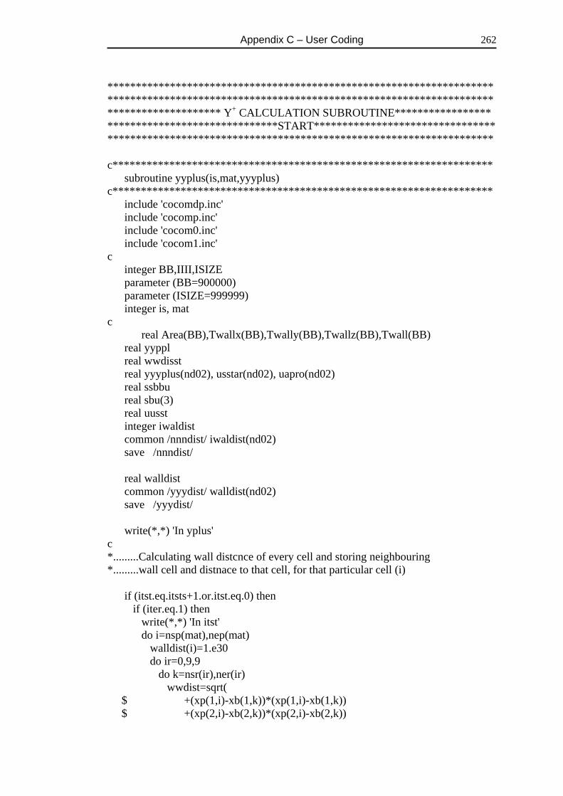
Appendix C – User Coding
262
******************************************************************** ******************************************************************** ******************** Y+ CALCULATION SUBROUTINE***************** ******************************START******************************** ******************************************************************** c******************************************************************* subroutine yyplus(is,mat,yyyplus) c******************************************************************* include 'cocomdp.inc' include 'cocomp.inc' include 'cocom0.inc' include 'cocom1.inc' c integer BB,IIII,ISIZE parameter (BB=900000) parameter (ISIZE=999999) integer is, mat c real Area(BB),Twallx(BB),Twally(BB),Twallz(BB),Twall(BB) real yyppl real wwdisst real yyyplus(nd02), usstar(nd02), uapro(nd02) real ssbbu real sbu(3) real uusst integer iwaldist common /nnndist/ iwaldist(nd02) save /nnndist/ real walldist common /yyydist/ walldist(nd02) save /yyydist/ write(*,*) 'In yplus' c *.........Calculating wall distcnce of every cell and storing neighbouring *.........wall cell and distnace to that cell, for that particular cell (i) if (itst.eq.itsts+1.or.itst.eq.0) then if (iter.eq.1) then write(*,*) 'In itst' do i=nsp(mat),nep(mat) walldist(i)=1.e30 do ir=0,9,9 do k=nsr(ir),ner(ir) wwdist=sqrt( $ +(xp(1,i)-xb(1,k))*(xp(1,i)-xb(1,k)) $ +(xp(2,i)-xb(2,k))*(xp(2,i)-xb(2,k))
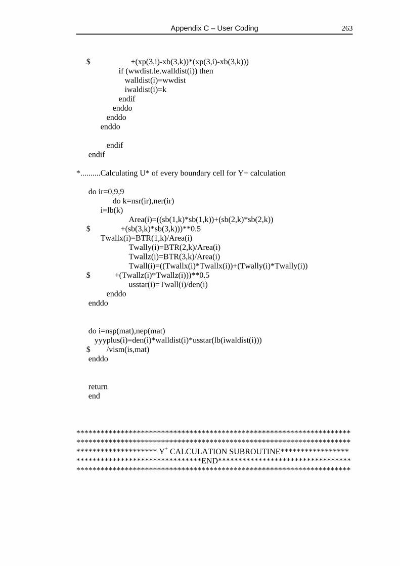
Appendix C – User Coding
263
$ +(xp(3,i)-xb(3,k))*(xp(3,i)-xb(3,k))) if (wwdist.le.walldist(i)) then walldist(i)=wwdist iwaldist(i)=k endif enddo enddo enddo endif endif *..........Calculating U* of every boundary cell for Y+ calculation do ir=0,9,9 do k=nsr(ir),ner(ir) i=lb(k) Area(i)=((sb(1,k)*sb(1,k))+(sb(2,k)*sb(2,k)) $ +(sb(3,k)*sb(3,k)))**0.5 Twallx(i)=BTR(1,k)/Area(i) Twally(i)=BTR(2,k)/Area(i) Twallz(i)=BTR(3,k)/Area(i) Twall(i)=((Twallx(i)*Twallx(i))+(Twally(i)*Twally(i)) $ +(Twallz(i)*Twallz(i)))**0.5 usstar(i)=Twall(i)/den(i) enddo enddo do i=nsp(mat),nep(mat) yyyplus(i)=den(i)*walldist(i)*usstar(lb(iwaldist(i))) $ /vism(is,mat) enddo return end ******************************************************************** ******************************************************************** ******************** Y+ CALCULATION SUBROUTINE***************** *******************************END********************************* ********************************************************************
Appendix D – LES Coding
264
Appendix D
LES Coding This appendix contains the subroutines for Smagorinsky model, Wall Adapting Eddy Viscosity model and the Dynamic Smagorinsky Model.
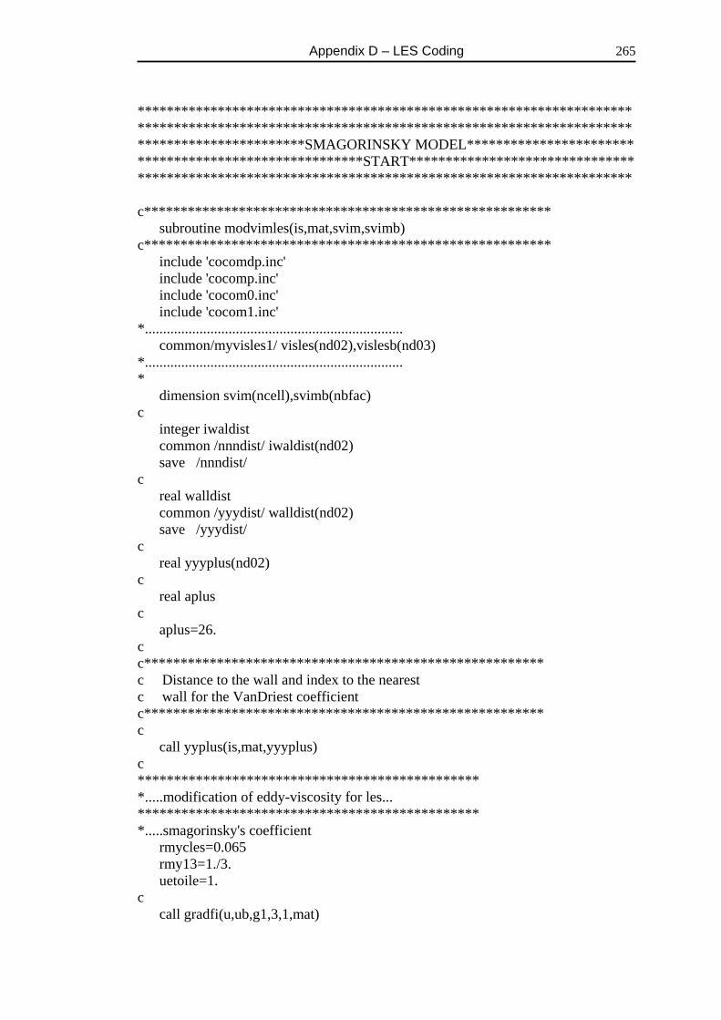
Appendix D – LES Coding
265
******************************************************************** ******************************************************************** ***********************SMAGORINSKY MODEL*********************** *******************************START******************************* ******************************************************************** c******************************************************** subroutine modvimles(is,mat,svim,svimb) c******************************************************** include 'cocomdp.inc' include 'cocomp.inc' include 'cocom0.inc' include 'cocom1.inc' *....................................................................... common/myvisles1/ visles(nd02),vislesb(nd03) *....................................................................... * dimension svim(ncell),svimb(nbfac) c integer iwaldist common /nnndist/ iwaldist(nd02) save /nnndist/ c real walldist common /yyydist/ walldist(nd02) save /yyydist/ c real yyyplus(nd02) c real aplus c aplus=26. c c******************************************************* c Distance to the wall and index to the nearest c wall for the VanDriest coefficient c******************************************************* c call yyplus(is,mat,yyyplus) c *********************************************** *.....modification of eddy-viscosity for les... *********************************************** *.....smagorinsky's coefficient rmycles=0.065 rmy13=1./3. uetoile=1. c call gradfi(u,ub,g1,3,1,mat)
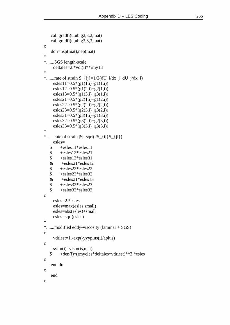
Appendix D – LES Coding
266
call gradfi(u,ub,g2,3,2,mat) call gradfi(u,ub,g3,3,3,mat) c do i=nsp(mat),nep(mat) * *.......SGS length-scale deltales=2.*vol(i)**rmy13 * *.......rate of strain S_ij=1/2(dU_i/dx_j+dU_j/dx_i) esles11=0.5*(g1(1,i)+g1(1,i)) esles12=0.5*(g1(2,i)+g2(1,i)) esles13=0.5*(g1(3,i)+g3(1,i)) esles21=0.5*(g2(1,i)+g1(2,i)) esles22=0.5*(g2(2,i)+g2(2,i)) esles23=0.5*(g2(3,i)+g3(2,i)) esles31=0.5*(g3(1,i)+g1(3,i)) esles32=0.5*(g3(2,i)+g2(3,i)) esles33=0.5*(g3(3,i)+g3(3,i)) * *.......rate of strain |S|=sqrt(2S_ijS_ji) esles= $ +esles11*esles11 $ +esles12*esles21 $ +esles13*esles31 & +esles21*esles12 $ +esles22*esles22 $ +esles23*esles32 & +esles31*esles13 $ +esles32*esles23 $ +esles33*esles33 c esles=2.*esles esles=max(esles,small) esles=abs(esles)+small esles=sqrt(esles) * *.......modified eddy-viscosity (laminar + SGS) c vdriest=1.-exp(-yyyplus(i)/aplus) c svim(i)=vism(is,mat) $ +den(i)*(rmycles*deltales*vdriest)**2.*esles c end do c end c

Appendix D – LES Coding
267
******************************************************************** ******************************************************************** ***********************SMAGORINSKY MODEL*********************** ********************************END******************************** ********************************************************************
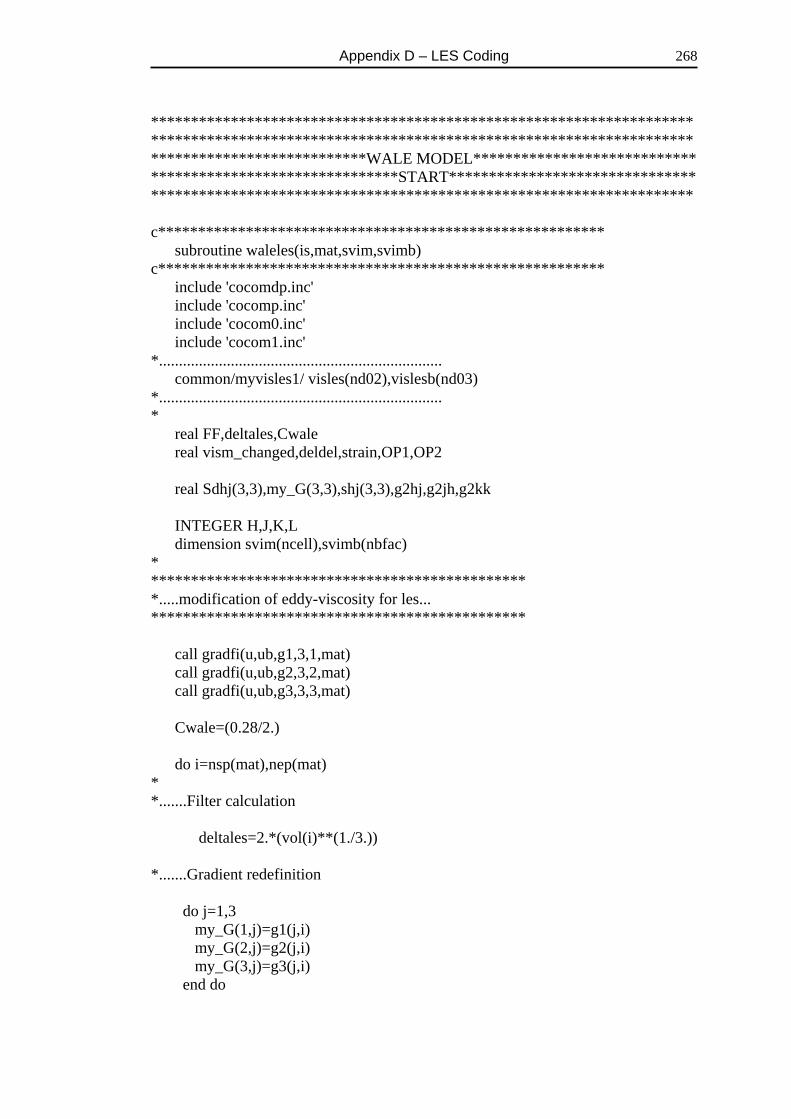
Appendix D – LES Coding
268
******************************************************************** ******************************************************************** ***************************WALE MODEL**************************** *******************************START******************************* ******************************************************************** c******************************************************** subroutine waleles(is,mat,svim,svimb) c******************************************************** include 'cocomdp.inc' include 'cocomp.inc' include 'cocom0.inc' include 'cocom1.inc' *....................................................................... common/myvisles1/ visles(nd02),vislesb(nd03) *....................................................................... * real FF,deltales,Cwale real vism_changed,deldel,strain,OP1,OP2 real Sdhj(3,3),my_G(3,3),shj(3,3),g2hj,g2jh,g2kk INTEGER H,J,K,L dimension svim(ncell),svimb(nbfac) * *********************************************** *.....modification of eddy-viscosity for les... *********************************************** call gradfi(u,ub,g1,3,1,mat) call gradfi(u,ub,g2,3,2,mat) call gradfi(u,ub,g3,3,3,mat) Cwale=(0.28/2.) do i=nsp(mat),nep(mat) * *.......Filter calculation deltales=2.*(vol(i)**(1./3.)) *.......Gradient redefinition do j=1,3 my_G(1,j)=g1(j,i) my_G(2,j)=g2(j,i) my_G(3,j)=g3(j,i) end do
Appendix D – LES Coding
269
strain=0.0 deldel=0.0 do h=1,3 do j=1,3 g2hj=0.0 g2jh=0.0 g2kk=0.0 do k=1,3 g2hj= g2hj+(my_G(h,k)*my_G(k,j)) g2jh= g2jh+(my_G(j,k)*my_G(k,h)) g2kk= g2kk+(my_G(k,k)*my_G(k,k)) end do !k shj(h,j)=0.5*(my_G(h,j)+my_G(j,h)) sdhj(h,j)=0.5*(g2hj+g2jh) end do !j sdhj(h,h)=sdhj(h,h)-((1./3.)*(g2kk)) do j=1,3 strain=strain+(shj(h,j)*shj(h,j)) deldel=deldel+(sdhj(h,j)*sdhj(h,j)) end do !j end do !h OP1=(deldel**(3./2.)) OP2=(strain**(5./2.))+(deldel**(5./4.)) OP2=Op2+small FF=OP1/OP2 vism_changed=((Cwale*deltales)**2.)*FF c if (i.eq.25) then c write(*,*)i,Cwale,deltales,FF,vism_changed c end if c if (i.eq.3067) then C write(*,*)i,Cwale,deltales,FF,vism_changed C end if C if (i.eq.3015) then C write(*,*)i,Cwale,deltales,FF,vism_changed C end if

Appendix D – LES Coding
270
*......Modified Eddy Viscosity (Laminar + den* SGS) svim(i)=vism(is,mat)+den(i)*vism_changed end do end ******************************************************************** ******************************************************************** ***************************WALE MODEL**************************** ********************************END******************************** ********************************************************************
Appendix D – LES Coding
271
******************************************************************** ******************************************************************** *******************DYNAMIC SMAGORINSKY MODEL***************** *******************************START******************************* ******************************************************************** c******************************************************** subroutine dynamic(is,mat,svim,svimb) c******************************************************** * Assign Global Cs and Csb * Initialize Gradients gl(l,i) * Assign Boundry gradients glb(i,lb(k)) * Calculate ui*uj and uib*ujb * Initialize (ui*uj)_Efil and gl(l,i)_Efil * Calculate ui_Efil, uj_Efil * Calculate (ui*uj)_Efil * Calculate Lij = (ui*uj)_Efil - (ui_Efil * uj_Efil) * Calculate Betaij and Bijb * Calculate Betaij_Efil * Calcualte gl(l,i)_Efil and glb(l,lb(k))_Efil * Calculate alphaij * Calcualte Mij = alphaij - Betaij_Efil * Calculate CsL = (Lij * Mij)/ (Mij * Mij) * Time Average Cs = Cs * (1-zeta) + zeta * CsL * Where zeta = DelT/TAve, and TAve = n * delT * where n = number of samples taken lets say 100 * Clipping Cs, 0 < Cs < 0.23 * Calculate Viscosity by LES Smagorinsky model * Screen Printing Some Variables * Filtering Subroutine *------------------------------------------------------------- * * ************************************************************** * Including Comet libraries for Variables declaration * include 'cocomdp.inc' include 'cocomp.inc' include 'cocom0.inc' include 'cocom1.inc' *------------------------------------------------------------- * * ************************************************************** * Variables Declaration for local code doubleprecision g1b(3,nd03), g2b(3,nd03), g3b(3,nd03) doubleprecision temp(nd02), tempb(nd03), tempg(nd02) doubleprecision denom, numer, zeta doubleprecision uiuj(3,3,nd02), uiujb(3,3,nd03)
Appendix D – LES Coding
272
doubleprecision Lij(3,3,nd02) doubleprecision betaij(3,3,nd02), betaijb(3,3,nd03) integer idir dimension svim(ncell),svimb(nbfac) *------------------------------------------------------------- * * ************************************************************** * Filtered variables declaration doubleprecision tmp(3,nd02), tmpb(3,nd03) doubleprecision tmpfil(3,nd02) doubleprecision ufil(3,nd02) doubleprecision uifujf(3,3,nd02) doubleprecision uiujfil(3,3,nd02) doubleprecision uifujfF(3,3,nd02) doubleprecision uifbujfb(3,3,nd03) doubleprecision g1fil(3,nd02) doubleprecision g2fil(3,nd02) doubleprecision g3fil(3,nd02) doubleprecision betaijfil(3,3,nd02) doubleprecision alphaij(3,3,nd02) doubleprecision Mij(3,3,nd02) integer nbnum(nd02) common/myvisc/c_dyn(nd02),c_dynb(nd03) integer i1, i2 doubleprecision fij doubleprecision ndisfi,ndisfib common/myvelmom1/ summtimes, $ summu(3,nd02),summub(3,nd03), $ summuu(3,3,nd02),summuub(3,3,nd03), $ summp(nd02),summpb(nd03) * *-------------------------------------------------------------- * * *************************************************************** ** Cell Neighbours checking here ** number of neighboures kk(i),and their indexes neighspeheres *************************************************************** common/myindint/kk(nd02), kkb(nd03),nsphere(nd02,1000), $ nbsphere(nd03,1000) common /myrelrel/ ndisfi(nd02,1000),ndisfib(nd03,1000) integer icount, nmax, z, zz doubleprecision sphere, tolxx,tolyy,tolzz logical fexist
Appendix D – LES Coding
273
write(*,*) 'In Dynamic' inquire(file='kk.dat',exist=fexist) if (.not.fexist) then open(92,file='kk.dat',status='unknown') do i=nsp(mat),nep(mat) tolxx=(3.14/32.0)*2.5 tolzz=(6.28/48.0)*2.5 tolyy=(vol(i)/(tolxx*tolzz))*3.1 c tolxx=(vol(i)**0.334)*2. c tolyy=(vol(i)**0.334)*2. c tolzz=(vol(i)**0.334)*2. c tolsphere=(((tolxx**2.)+(tolyy**2.)+(tolzz**2.))**0.5) icount=0 do j=nsp(mat),nep(mat) if (abs(xp(1,i)-xp(1,j)).lt.tolxx.and. & abs(xp(2,i)-xp(2,j)).lt.tolyy.and. & abs(xp(3,i)-xp(3,j)).lt.tolzz) then sphere=sqrt((xp(1,i)-xp(1,j))**2. & +(xp(2,i)-xp(2,j))**2. & +(xp(3,i)-xp(3,j))**2.) c if (sphere.le.tolsphere) then icount=icount+1 nsphere(i,icount)=j ndisfi(i,icount)=sphere c end if endif end do kk(i)=icount icount=0 do ir=0,nreg do k=nsr(ir),ner(ir) if (abs(xp(1,i)-xb(1,k)).lt.tolxx.and. & abs(xp(2,i)-xb(2,k)).lt.tolyy.and.
Appendix D – LES Coding
274
& abs(xp(3,i)-xb(3,k)).lt.tolzz) then sphere=sqrt((xp(1,i)-xb(1,k))**2. & +(xp(2,i)-xb(2,k))**2. & +(xp(3,i)-xb(3,k))**2.) c if (sphere.le.tolsphere) then icount=icount+1 nbsphere(i,icount)=k ndisfib(i,icount)=sphere c end if end if end do enddo kkb(i)=icount write(92,*) kk(i) do j=1,kk(i) write(92,*) nsphere(i,j),ndisfi(i,j) enddo write(92,*) kkb(i) do j=1,kkb(i) write(92,*) nbsphere(i,j),ndisfib(i,j) enddo enddo close(unit=92) else if ((ITST.eq.ITSTS+1).and.(ITER.eq.1)) then write(*,*) 'kk.dat' open(UNIT=92,FILE='kk.dat',status='old') do i=nsp(mat),nep(mat) read(92,*) kk(i) do j=1,kk(i) read(92,*) nsphere(i,j), ndisfi(i,j) enddo
Appendix D – LES Coding
275
read(92,*) kkb(i) do j=1,kkb(i) read(92,*) nbsphere(i,j), ndisfib(i,j) enddo enddo close(unit=92) endif *-------------------------------------------------------------- * * *************************************************************** rmy13=1./3. zeta=0.01 * *************************************************************** * Assigning Global Cs and Csb * write(*,*) 'Dynamic model for LES.',vism(is,mat),is,mat write(*,*) itst,itsts if (ITST.eq.1) then do i=nsp(mat),nep(mat) c_dyn(i)=4*(0.065**2) enddo do ir=0,nreg do k=nsr(ir),ner(ir) c_dynb(k)=0.00001 enddo enddo c*********************************************************************** c*********************************************************************** else if ((ITST.eq.ITSTS+1).and.(ITER.eq.1)) then write(*,*) 'Dyn_Cs.dat' open(79,file='Dyn_Cs.dat',status='unknown') c do mat=1,nmat do i=nsp(mat),nep(mat) read(79,*)n,svim(n),esles,c_dyn(n) enddo
Appendix D – LES Coding
276
c enddo close(79) do ir=0,nreg do k=nsr(ir),ner(ir) c_dynb(k)=0.0001 enddo enddo c*********************************************************************** endif *-------------------------------------------------------------- * * *************************************************************** * Initializing Gradients gl(l,i) * do l=1,3 do i=1,nd02 g1(l,i)=0. g2(l,i)=0. g3(l,i)=0. enddo enddo c*-------------------------------------------------------------- * * *************************************************************** * Calculating Boundry Gradients * call gradfi(u,ub,g1,3,1,mat) call gradfi(u,ub,g2,3,2,mat) call gradfi(u,ub,g3,3,3,mat) do ir=0,nreg do k=nsr(ir),ner(ir) g1b(1,k)=g1(1,lb(k)) g1b(2,k)=g1(2,lb(k)) g1b(3,k)=g1(3,lb(k)) g2b(1,k)=g2(1,lb(k)) g2b(2,k)=g2(2,lb(k)) g2b(3,k)=g2(3,lb(k)) g3b(1,k)=g3(1,lb(k)) g3b(2,k)=g3(2,lb(k)) g3b(3,k)=g3(3,lb(k)) end do end do *-------------------------------------------------------------- *
Appendix D – LES Coding
277
* * *************************************************************** * Calculate ui * uj and uib * ujb * * Calcualte ui * uj do l=1,3 do m=1,3 do i=nsp(mat),nep(mat) uiuj(l,m,i)=u(l,i)*u(m,i) end do enddo end do * Calculate uib * ujb * do l=1,3 do m=1,3 do ir=0,nreg do k=nsr(ir),ner(ir) uiujb(l,m,k)=ub(l,k)*ub(m,k) enddo enddo end do end do c*--------------------------------------------------------------- * * * **************************************************************** * Initialize (ui*uj)_Efil, Betaij_Efil, ui_Efil, gl(l,i)_Efil * * Initializing (ui*uj)_Efil and Betaij_Efil do l=1,3 do i=nsp(mat),nep(mat) do m=1,3 uiujfil(l,m,i)=0. betaijfil(l,m,i)=0. end do * Initiallizing ui_Efil and gl(l,i)_Efil ufil(l,i)=0. g1fil(l,i)=0. g2fil(l,i)=0. g3fil(l,i)=0. nbnum(i)=0 end do

Appendix D – LES Coding
278
end do *.....Number of faces per cell (to be checked) (nd01=number of faces) do j=1,nd01 j1=lf(1,j) nbnum(j1)=nbnum(j1)+1 j2=lf(2,j) nbnum(j2)=nbnum(j2)+1 enddo do ir=0,nreg do k=nsr(ir),ner(ir) j1=lb(k) nbnum(j1)=nbnum(j1)+1 enddo enddo *-------------------------------------------------------------------- * * * ********************************************************************* * Calculate ui_Efil and uj_Efil * *.....Filtered quantities are calculated as the mean of their *.....value at the face centres. *.....Explicit filtering of the velocity and the velocity product * * do l=1,3 do i=1,nd02 tmp(l,i)=u(l,i) enddo do k=1,nd03 tmpb(l,k)=ub(l,k) enddo enddo call filter(tmp,tmpb,nbnum,tmpfil,mat) do l=1,3 do i=1,nd02 ufil(l,i)=tmpfil(l,i) c write(*,*) ufil(l,i),u(l,i),ufil(l,i)-u(l,i),l,i
Appendix D – LES Coding
279
enddo enddo * c do i=1,nd02 c write(84,*) xp(1,i),xp(2,i),xp(3,i), c $ u(1,i),ufil(1,i),u(2,i),ufil(2,i),u(3,i),ufil(3,i) c enddo c stop *-------------------------------------------------------------------- * * * ********************************************************************* * Calculate (ui * uj)_Efil * do m=1,3 do l=1,3 do i=1,nd02 tmp(l,i)=uiuj(l,m,i) enddo do k=1,nd03 tmpb(l,k)=uiujb(l,m,k) enddo enddo call filter(tmp,tmpb,nbnum,tmpfil,mat) do l=1,3 do i=1,nd02 uiujfil(l,m,i)=tmpfil(l,i) enddo enddo enddo *-------------------------------------------------------------------- * * * ********************************************************************* * Calculate Lij = (ui*uj)_Efil - (ui_Efil * uj_Efil) * do l=1,3 do m=1,3 do i=nsp(mat),nep(mat) Lij(l,m,i)=uiujfil(l,m,i)-(ufil(l,i)*ufil(m,i))
Appendix D – LES Coding
280
end do end do end do * *-------------------------------------------------------------------- * * * ********************************************************************* * Calculation of beta_ij, and betaijb * * Calcualte beta_ij do i=nsp(mat),nep(mat) * *........SGS length-scale * deltales=2.*(vol(i)**rmy13) * *........rate of strain S_ij=1/2(dU_i/dx_j+dU_j/dx_i) * esles11=0.5*(g1(1,i)+g1(1,i)) esles12=0.5*(g1(2,i)+g2(1,i)) esles13=0.5*(g1(3,i)+g3(1,i)) esles21=0.5*(g2(1,i)+g1(2,i)) esles22=0.5*(g2(2,i)+g2(2,i)) esles23=0.5*(g2(3,i)+g3(2,i)) esles31=0.5*(g3(1,i)+g1(3,i)) esles32=0.5*(g3(2,i)+g2(3,i)) esles33=0.5*(g3(3,i)+g3(3,i)) * *........rate of strain |S|=sqrt(2S_ijS_ij) * esles=esles11*esles11+esles12*esles12+esles13*esles13+ & esles21*esles21+esles22*esles22+esles23*esles23+ & esles31*esles31+esles32*esles32+esles33*esles33 esles=2.*esles esles=max(esles,small) esles=abs(esles)+small esles=sqrt(esles) betaij(1,1,i)=deltales*deltales*esles*esles11 betaij(1,2,i)=deltales*deltales*esles*esles12 betaij(1,3,i)=deltales*deltales*esles*esles13 betaij(2,1,i)=deltales*deltales*esles*esles21 betaij(2,2,i)=deltales*deltales*esles*esles22 betaij(2,3,i)=deltales*deltales*esles*esles23 betaij(3,1,i)=deltales*deltales*esles*esles31
Appendix D – LES Coding
281
betaij(3,2,i)=deltales*deltales*esles*esles32 betaij(3,3,i)=deltales*deltales*esles*esles33 * end do * Calculate betaijb do ir=0,nreg do k=nsr(ir),ner(ir) i1=lb(k) *...........SGS length-scale * deltales=2.*(vol(i1)**rmy13) * *...........rate of strain S_ij=1/2(dU_i/dx_j+dU_j/dx_i) * esles11=0.5*(g1b(1,k)+g1b(1,k)) esles12=0.5*(g1b(2,k)+g2b(1,k)) esles13=0.5*(g1b(3,k)+g3b(1,k)) esles21=0.5*(g2b(1,k)+g1b(2,k)) esles22=0.5*(g2b(2,k)+g2b(2,k)) esles23=0.5*(g2b(3,k)+g3b(2,k)) esles31=0.5*(g3b(1,k)+g1b(3,k)) esles32=0.5*(g3b(2,k)+g2b(3,k)) esles33=0.5*(g3b(3,k)+g3b(3,k)) * *...........rate of strain |S|=sqrt(2S_ijS_ij) * esles= $ esles11*esles11+esles12*esles12+esles13*esles13+ $ esles21*esles21+esles22*esles22+esles23*esles23+ $ esles31*esles31+esles32*esles32+esles33*esles33 esles=2.*esles esles=max(esles,small) esles=abs(esles)+small esles=sqrt(esles) betaijb(1,1,k)=deltales*deltales*esles*esles11 betaijb(1,2,k)=deltales*deltales*esles*esles12 betaijb(1,3,k)=deltales*deltales*esles*esles13 betaijb(2,1,k)=deltales*deltales*esles*esles21 betaijb(2,2,k)=deltales*deltales*esles*esles22 betaijb(2,3,k)=deltales*deltales*esles*esles23 betaijb(3,1,k)=deltales*deltales*esles*esles31 betaijb(3,2,k)=deltales*deltales*esles*esles32 betaijb(3,3,k)=deltales*deltales*esles*esles33
Appendix D – LES Coding
282
end do enddo *-------------------------------------------------------------------- * * * ********************************************************************* * Calcualte Betaij_Efil do m=1,3 do l=1,3 do i=1,nd02 tmp(l,i)=betaij(l,m,i) enddo do k=1,nd03 tmpb(l,k)=betaijb(l,m,k) enddo enddo call filter(tmp,tmpb,nbnum,tmpfil,mat) do l=1,3 do i=1,nd02 betaijfil(l,m,i)=tmpfil(l,i) enddo enddo enddo *--------------------------------------------------------------------- * * * ********************************************************************** * Calculate gl(l,i) and glb(l,lb(k)) * * Calcualte g1(l,i) and g1b(l,lb(k)) do l=1,3 do i=1,nd02 tmp(l,i)=g1(l,i) enddo do k=1,nd03 tmpb(l,k)=g1b(l,k) enddo enddo
Appendix D – LES Coding
283
call filter(tmp,tmpb,nbnum,tmpfil,mat) do l=1,3 do i=1,nd02 g1fil(l,i)=tmpfil(l,i) enddo enddo * Calcualte g2(l,i) and g2b(l,lb(k)) do l=1,3 do i=1,nd02 tmp(l,i)=g2(l,i) enddo do k=1,nd03 tmpb(l,k)=g2b(l,k) enddo enddo call filter(tmp,tmpb,nbnum,tmpfil,mat) do l=1,3 do i=1,nd02 g2fil(l,i)=tmpfil(l,i) enddo enddo * Calcualte g3(l,i) and g3b(l,lb(k)) do l=1,3 do i=1,nd02 tmp(l,i)=g3(l,i) enddo do k=1,nd03 tmpb(l,k)=g3b(l,k) enddo enddo call filter(tmp,tmpb,nbnum,tmpfil,mat) do l=1,3 do i=1,nd02 g3fil(l,i)=tmpfil(l,i) enddo enddo *-------------------------------------------------------------------- * * *
Appendix D – LES Coding
284
********************************************************************* * Calculate alpha_ij * do i=nsp(mat),nep(mat) * *........Explicit filtered length-scale * deltalesfil=4.*(vol(i)**rmy13) * *........Filtered rate of strain S_ij=1/2(dU_i/dx_j+dU_j/dx_i) * esles11=0.5*(g1fil(1,i)+g1fil(1,i)) esles12=0.5*(g1fil(2,i)+g2fil(1,i)) esles13=0.5*(g1fil(3,i)+g3fil(1,i)) esles21=0.5*(g2fil(1,i)+g1fil(2,i)) esles22=0.5*(g2fil(2,i)+g2fil(2,i)) esles23=0.5*(g2fil(3,i)+g3fil(2,i)) esles31=0.5*(g3fil(1,i)+g1fil(3,i)) esles32=0.5*(g3fil(2,i)+g2fil(3,i)) esles33=0.5*(g3fil(3,i)+g3fil(3,i)) * *........Filetered rate of strain |S|=sqrt(2S_ijS_ij) * esles= $ esles11*esles11+esles12*esles12+esles13*esles13+ $ esles21*esles21+esles22*esles22+esles23*esles23+ $ esles31*esles31+esles32*esles32+esles33*esles33 esles=2.*esles esles=max(esles,small) esles=abs(esles)+small esles=sqrt(esles) alphaij(1,1,i)=deltalesfil*deltalesfil*esles*esles11 alphaij(1,2,i)=deltalesfil*deltalesfil*esles*esles12 alphaij(1,3,i)=deltalesfil*deltalesfil*esles*esles13 alphaij(2,1,i)=deltalesfil*deltalesfil*esles*esles21 alphaij(2,2,i)=deltalesfil*deltalesfil*esles*esles22 alphaij(2,3,i)=deltalesfil*deltalesfil*esles*esles23 alphaij(3,1,i)=deltalesfil*deltalesfil*esles*esles31 alphaij(3,2,i)=deltalesfil*deltalesfil*esles*esles32 alphaij(3,3,i)=deltalesfil*deltalesfil*esles*esles33 end do * *------------------------------------------------------------------- * * *
Appendix D – LES Coding
285
******************************************************************** * Calculate Mij do l=1,3 do m=1,3 do i=nsp(mat),nep(mat) Mij(l,m,i)=(alphaij(l,m,i)-betaijfil(l,m,i)) end do end do end do *------------------------------------------------------------------- * * * ******************************************************************** * Calculate CsL by lillys least sqare method * sumtimes=float(iter) sumtimes=float(maxit)*summtimes+sumtimes write(*,*) sumtimes open(89,file='Dyn_Cs.dat',status='unknown') do i=nsp(mat),nep(mat) denom=0. numer=0. do l=1,3 do m=1,3 cdyn=cdyn+(0.5*((Lij(l,m,i)*Mij(l,m,i))/ $ ((Mij(l,m,i)*Mij(l,m,i))+small))) end do end do * Moving Time Average of CsL c cdyn=-0.5*numer/(denom+small) c c c_dyn(i)=(cdyn+c_dyn(i))/2 c c_dyn(i)=((1-zeta)*c_dyn(i))+(zeta*cdyn) c_dyn(i)=-cdyn * * Calculate Gradients for Dynamic Smagorensky Model * deltales=2.*(vol(i)**rmy13) * *........rate of strain S_ij=1/2(dU_i/dx_j+dU_j/dx_i) * esles11=0.5*(g1(1,i)+g1(1,i)) esles12=0.5*(g1(2,i)+g2(1,i))
Appendix D – LES Coding
286
esles13=0.5*(g1(3,i)+g3(1,i)) esles21=0.5*(g2(1,i)+g1(2,i)) esles22=0.5*(g2(2,i)+g2(2,i)) esles23=0.5*(g2(3,i)+g3(2,i)) esles31=0.5*(g3(1,i)+g1(3,i)) esles32=0.5*(g3(2,i)+g2(3,i)) esles33=0.5*(g3(3,i)+g3(3,i)) * *........rate of strain |S|=sqrt(2S_ijS_ij) * esles= $ esles11*esles11+esles12*esles12+esles13*esles13+ $ esles21*esles21+esles22*esles22+esles23*esles23+ $ esles31*esles31+esles32*esles32+esles33*esles33 esles=2.*esles esles=max(esles,small) esles=abs(esles)+small esles=sqrt(esles) * *........modified eddy-viscosity (laminar + SGS) * * Clipping Cs, 0 < Cs < 0.23 if (c_dyn(i).le.0.0) then c_dyn(i)=0.000001 endif if (c_dyn(i).ge.0.06) then c_dyn(i)=0.06 endif * Calculate Viscosity by Dynamic Smagorinsky Model svim(i)=vism(is,mat)+(den(i)*c_dyn(i)*(deltales**2.0)*esles) write(89,*)i,svim(i),esles,c_dyn(i) end do close(89) c 555 format(i16,2x,f13.9,2x,f13.9,2x,f13.9) *--------------------------------------------------------------------- *--------------------------------------------------------------------- * Program Terminates here end *---------------------------------------------------------------------- **************************************************************** ********************NEW FILTERING SUBROUTIE ******************* **************************************************************** subroutine filter(tmp,tmpb,nbnum,tmpfil,mat)
Appendix D – LES Coding
287
include 'cocomdp.inc' include 'cocomp.inc' include 'cocom0.inc' include 'cocom1.inc' *....................................................................... * integer mat integer nbnum(nd02) doubleprecision fij doubleprecision tmp(3,nd02), tmpb(3,nd03) doubleprecision tmpfil(3,nd02) doubleprecision ndisfi,ndisfib common/myindint/kk(nd02), kkb(nd03),nsphere(nd02,1000), $ nbsphere(nd03,1000) common /myrelrel/ ndisfi(nd02,1000),ndisfib(nd03,1000) doubleprecision susunum,susuden,susu do l=1,3 do i=nsp(mat),nep(mat) susunum=0. susuden=0. do n=1,kk(i) if (ndisfi(i,n).eq.0.0) then susunum=susunum susuden=susuden else susunum=susunum+(tmp(l,nsphere(i,n))/(ndisfi(i,n))) susuden=susuden+(1./(ndisfi(i,n))) end if end do do n=1,kkb(i) if (ndisfib(i,n).eq.0.0) then susunum=susunum susuden=susuden else susunum=susunum+(tmpb(l,nbsphere(i,n))/(ndisfib(i,n))) susuden=susuden+(1./(ndisfib(i,n))) end if end do tmpfil(l,i)=(susunum/(susuden+small)) end do

Appendix D – LES Coding
288
end do return end ******************************************************************** ******************************************************************** *******************DYNAMIC SMAGORINSKY MODEL***************** ********************************END******************************** ********************************************************************

Appendix E - Car Mirror
289
Appendix E
Car Mirror This section contains comparisons of the car mirror results with experimental measurements. The experimental setup details are given below. Diameter of mirror: 0.2 m Aspect Ratio: 1.5 Inlet velocity: 26 m/s
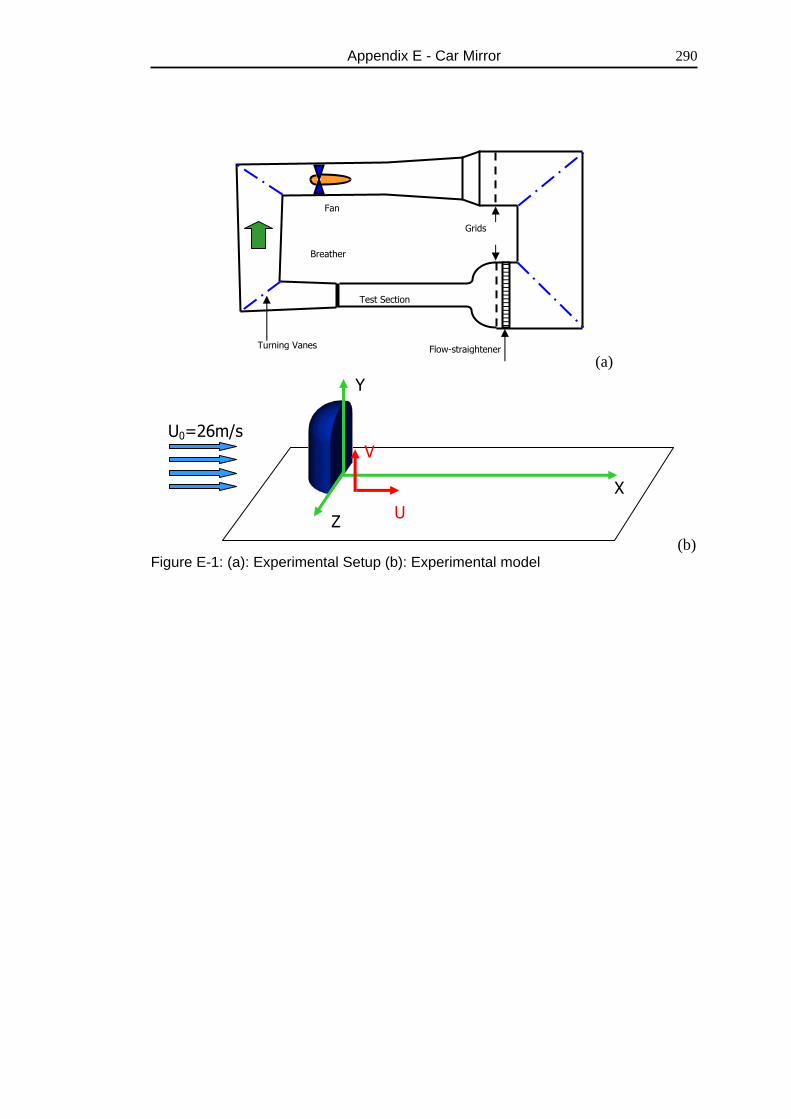
Appendix E - Car Mirror
290
(a)
(b) Figure E-1: (a): Experimental Setup (b): Experimental model
X
Y
Z U
V U0=26m/s
Fan
Test Section
Grids
Breather
Flow-straightenerTurning Vanes